DRAFT

Miller, L. A. and Peskin, C. S.

Title: Flexible clap and fling in tiny insect flight.

Abstract

Many of the smallest flying insects clap their wings together at the end of each upstroke

and fling them apart at the end of each downstroke to augment the lift forces generated

during flight. Previous work using rigid wings has shown that at low Reynolds numbers,

this mechanism is rather inefficient as large drag forces are produced when the wings are

clapped together and pulled apart. In this paper, we have used the immersed boundary

method to investigate whether or not wing flexibility improves aerodynamic performance

during low Reynolds number ‘clap and fling.’ Our results suggest, for a certain range of

flexibilities, that wings with rigid leading edges and flexible trailing edges yield

improved aerodynamic performance relative to the rigid wing case. Different wing

designs are also shown to yield improved lift generation or improved aerodynamic

efficiency.

Introduction

It has been proposed that the smallest flying insects augment the lift forces generated

during flight by clapping their wings together at the end of each upstroke and then

flinging them apart at the beginning of each downstroke (Ellington, 1984; Lighthill,

1973; Weis-Fogh, 1973). At these low Reynolds numbers (Re), lift is augmented during

wing rotation (fling) and subsequent translation by the formation of two large leading

edge vortices (Miller and Peskin, 2005; Sun and Tang, 2003). The cost of this behavior is

that relatively large forces are required to initially fling the wings apart, and the relative

magnitude of these forces drastically increases with decreasing Re. For rigid wings, the

lift to drag ratios produced during clap and fling are lower than the ratios for the

corresponding one wing case, although the absolute lift forces generated are larger. For

the smallest insects, the forces required to fling the wings are so large that it begs the

question of why tiny insects clap and fling in the first place.

One major assumption in previous clap and fling studies using physical models

(Lehmann et al., 2005; Maxworthy, 1979; Spedding and Maxworthy, 1986; Sunada et al.,

1993), mathematical models (Lighthill, 1973), and numerical simulations (Miller and

Peskin, 2005; Sun and Tang, 2003) is that the wings are rigid. It seems likely that wing

flexibility could allow the wings reconfigure to lower drag profiles during clap and fling.

In this case, the fling might appear more like a 'peel,' and the clap might be thought of as

a reverse peel (Ellington, 1984). A number of studies support the idea that flexibility

allows for reconfiguration of biological structures, which results in reduced drag forces

experienced by the organisms (for example, Koehl, 1984; Vogel, 1989; Denny 1994;

Etnier and Vogel, 2000; Alben et al., 2002, 2004). The basic idea in these cases is that the

force on the body produced by the moving fluid causes the flexible body to bend or

reconfigure which, in turn, reduces the force felt by the body.

Ellington (1984) suggested that such a peel mechanism might serve to augment lift forces

relative to the rigid-fling case. In the case of peel, the wings are pulled apart along the

leading edges and curve along the wing chords. As the peel progresses, the separation

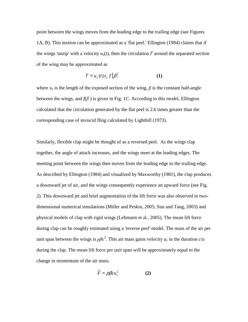
point between the wings moves from the leading edge to the trailing edge (see Figures

1A, B). This motion can be approximated as a 'flat peel.' Ellington (1984) claims that if

the wings 'unzip' with a velocity uz(t), then the circulation Γ

around the separated section

of the wing may be approximated as

( ) (1) )( βfxtu ez=Γ

where xe is the length of the exposed section of the wing, β is the constant half-angle

between the wings, and f(β ) is given in Fig. 1C. According to this model, Ellington

calculated that the circulation generated by the flat peel is 2.6 times greater than the

corresponding case of inviscid fling calculated by Lighthill (1973).

Similarly, flexible clap might be thought of as a reversed peel. As the wings clap

together, the angle of attack increases, and the wings meet at the leading edges. The

meeting point between the wings then moves from the leading edge to the trailing edge.

As described by Ellington (1984) and visualized by Maxworthy (1981), the clap produces

a downward jet of air, and the wings consequently experience an upward force (see Fig.

2). This downward jet and brief augmentation of the lift force was also observed in two-

dimensional numerical simulations (Miller and Peskin, 2005; Sun and Tang, 2003) and

physical models of clap with rigid wings (Lehmann et al., 2005). The mean lift force

during clap can be roughly estimated using a 'reverse peel' model. The mass of the air per

unit span between the wings is ρ β c2. This air mass gains velocity uc in the duration c/u

during the clap. The mean lift force per unit span will be approximately equal to the

change in momentum of the air mass.

(2) 2ccuF ρβ=

This is an inviscid approximation of the mean force, and the force generated in the

viscous case is likely to be smaller since some momentum is lost to viscosity.

In this paper, we have used computational fluid dynamics to study the effects of wing

flexibility on the forces produced during clap and fling. The immersed boundary method

was used to model pairs of rigid and flexible wings performing a two-dimensional clap

and fling stroke at Re = 10. The cases of flexible clap and peel were compared to the

cases of rigid clap and fling. Lift and drag coefficients were calculated as functions of

time and related to the behavior of the wing and the relative strengths of the leading and

trailing edge vortices.

Methods

The numerical method

The Immersed Boundary Method has been used successfully to model a variety of

problems in biological fluid dynamics. Such problems usually involve the interactions

between incompressible viscous fluids and deformable elastic boundaries. Some

examples of biological problems that have been studied with the Immersed Boundary

Method include aquatic animal locomotion (Fauci and Peskin, 1988; Fauci, 1990; Fauci

and Fogelson, 1993), cardiac blood flow (Peskin, 1977; Peskin and McQueen, 1996;

McQueen and Peskin, 2000), and ciliary driven flows (Grunbaum et al., 1998).

The equations of motion for a two-dimensional fluid are as follows:

( ) ( ) ( ) ( ) ( ) ( ) (3)xFxuxxuxuxu

,,,p,,,

tttttt

t +∆+−∇=

∇•+

∂∂ µρ

( ) (4) xu 0, =•∇ t

where u(x, t) is the fluid velocity, p(x, t) is the pressure, F(x, t) is the force per unit area

applied to the fluid by the immersed wing, ρ is the density of the fluid, and � is the

dynamic viscosity of the fluid. The independent variables are the time t and the position

x. Note that bold letters represent vector quantities. Eqns. 3 and 4 are the Navier-Stokes

equations for viscous flow in Eulerian form. Eqn. 4 is the condition that the fluid is

incompressible.

The interaction equations between the fluid and the boundary are given by:

( ) ( )( ) (5) XxfxF ,),(, drtrtrt ∫ −= δ

( ) ( )( ) ( ) ( )( ) (6) xXxxuXUX

,,,,

∫ −==∂

∂dtrttr

t

tr δ

where f(r, t) is the force per unit length applied by the wing to the fluid as a function of

Lagrangian position and time, δ(x) is a two-dimensional delta function, X(r, t) gives the

Cartesian coordinates at time t of the material point labeled by the Lagrangian parameter

r. Eqn. 5 applies force from the boundary to the fluid grid, and Eqn. 6 evaluates the local

fluid velocity at the boundary. The boundary is then moved at the local fluid velocity,

and this enforces the no-slip condition. Each of these equations involves a two-

dimensional Dirac delta function δ , which acts in each case as the kernel of an integral

transformation. These equations convert Lagrangian variables to Eulerian variables and

vice versa.

The immersed boundary equations are given by:

( ) ( ) ( )( ) (7) XYf ,,, targtarg trtrktr −=

( ) ( )(8)

Xf

,,

4

4

beambeam r

trktr

∂∂−=

(9)X

XXf

),(

),( 1),( strstr

∂∂∂∂

−

∂∂

∂∂=

rtr

rtr

rrktr

( ) ( ) ( ) (10) ffff ),( ,,, strbeamtarg trtrtrtr ++=

These equations describe the forces applied to the fluid by the boundary in Lagrangian

coordinates. Eqn. 7 describes the force applied to the fluid as a result of the target

boundary. ftarg(r, t) is the external force per unit length applied to the wing, ktarg is a

stiffness coefficient, and Y(r, t) gives the desired motion of the wing. Eqn. 8 describes

the force applied to the fluid as a result of the deformation of the actual boundary which

is here modeled as a beam. fbeam(r, t) is the force per unit length and kbeam is a stiffness

coefficient. Eqn. 9 describes the force applied to the fluid as a result of the resistance to

stretching by boundary given as fstr(r, t) where kstr is the corresponding stiffness

coefficient. Finally, Eqn. 10 describes the total force applied to the fluid per unit length,

f(r, t), as a result of both the target boundary and the deformation of the boundary.

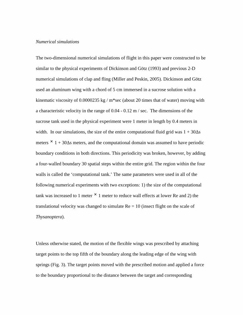
Numerical simulations

The two-dimensional numerical simulations of flight in this paper were constructed to be

similar to the physical experiments of Dickinson and Götz (1993) and previous 2-D

numerical simulations of clap and fling (Miller and Peskin, 2005). Dickinson and Götz

used an aluminum wing with a chord of 5 cm immersed in a sucrose solution with a

kinematic viscosity of 0.0000235 kg / m*sec (about 20 times that of water) moving with

a characteristic velocity in the range of 0.04 - 0.12 m / sec. The dimensions of the

sucrose tank used in the physical experiment were 1 meter in length by 0.4 meters in

width. In our simulations, the size of the entire computational fluid grid was 1 + 30� s

meters × 1 + 30� s meters, and the computational domain was assumed to have periodic

boundary conditions in both directions. This periodicity was broken, however, by adding

a four-walled boundary 30 spatial steps within the entire grid. The region within the four

walls is called the ‘computational tank.’ The same parameters were used in all of the

following numerical experiments with two exceptions: 1) the size of the computational

tank was increased to 1 meter × 1 meter to reduce wall effects at lower Re and 2) the

translational velocity was changed to simulate Re = 10 (insect flight on the scale of

Thysanoptera).

Unless otherwise stated, the motion of the flexible wings was prescribed by attaching

target points to the top fifth of the boundary along the leading edge of the wing with

springs (Fig. 3). The target points moved with the prescribed motion and applied a force

to the boundary proportional to the distance between the target and corresponding

boundary points. The bottom 4/5 of the wing (trailing edge) was free to bend. This has

the effect of modeling a flexible wing with a rigid leading edge. In the 'nearly-rigid' case,

springs were attached to target points along the entire length of the wing which prevented

any significant deformation. The stiffness coefficient of the springs that attach the

boundary points to the target points was ktarg = 1.44 ×105 kg / s2, and the stiffness

coefficient for the tension or compression of the wing was also set to kstr = 1.44 ×105 kg /

s2. These values were chosen to prevent any significant stretching or deformation of the

wings in the rigid case.

The flexural or bending stiffness of the wing was varied from 0.125 to 2 κ 2/ mN , where κ = 5.5459 610−× 2/ mN . This choice of flexural stiffness is not directly related to the

actual stiffness of insect wings since the numerical simulation is actually based on a

dynamically scaled physical model of insect flight. We chose this value of κ to represent

the case where deformations during translation are minimal, but bending does occur

when the wings are close. Ellington (1984) notes that the deformations of thrips’ wings

due to aerodynamic and inertial forces are minimal when vibrated at the frequency and

amplitude characteristic of flight. Since the maximum forces experienced by the wings

during clap and fling at Re=10 are significantly larger than the forces experienced during

one-winged translation (see Results), it seems possible that some bending would occur

when the wings are pressed together or peeled apart. Combes and Daniels (2003) showed

that much of the wing deformation observed during the flight of the hawkmoth Manduca

sexta is actually due to inertial rather than aerodynamic forces. They also predict that the

same would be true for smaller flying insects. Ellington’s experiments, however, show

that wing deformations due to inertial forces in thrips are small. Since accelerations are

comparable in the two-winged case, the effect of inertial forces on wing bending during

clap and fling should also be small.

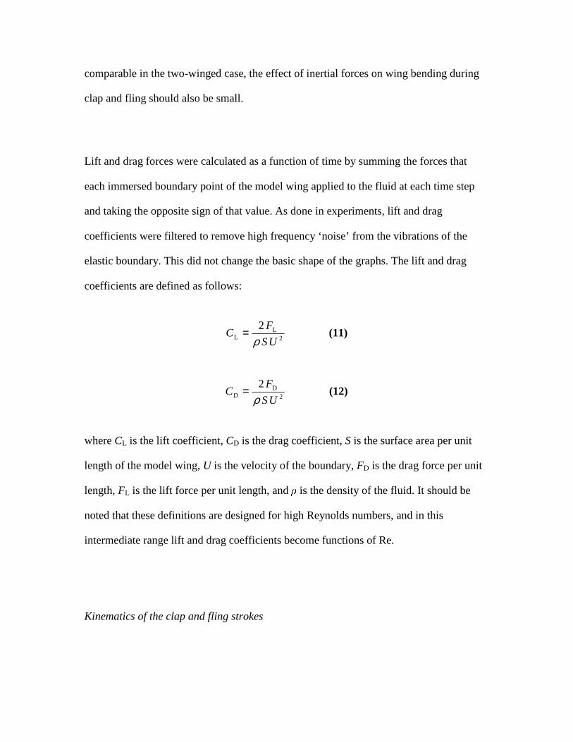
Lift and drag forces were calculated as a function of time by summing the forces that

each immersed boundary point of the model wing applied to the fluid at each time step

and taking the opposite sign of that value. As done in experiments, lift and drag

coefficients were filtered to remove high frequency ‘noise’ from the vibrations of the

elastic boundary. This did not change the basic shape of the graphs. The lift and drag

coefficients are defined as follows:

(11) 2

2L

L US

FC

ρ=

(12) 2

2D

D US

FC

ρ=

where CL is the lift coefficient, CD is the drag coefficient, S is the surface area per unit

length of the model wing, U is the velocity of the boundary, FD is the drag force per unit

length, FL is the lift force per unit length, and ρ is the density of the fluid. It should be

noted that these definitions are designed for high Reynolds numbers, and in this

intermediate range lift and drag coefficients become functions of Re.

Kinematics of the clap and fling strokes

Since the aerodynamic effects of previous strokes at Re=10 are minimal (Miller and

Peskin, 2005), either a single clap upstroke or a single fling downstroke was simulated.

The kinematics of the left wing during the clap strokes (upstrokes) are described here.

The right wing (when present) was the mirror image of the left wing at all times during

its motion, and the kinematics of the fling (downstroke) was symmetric to the upstroke.

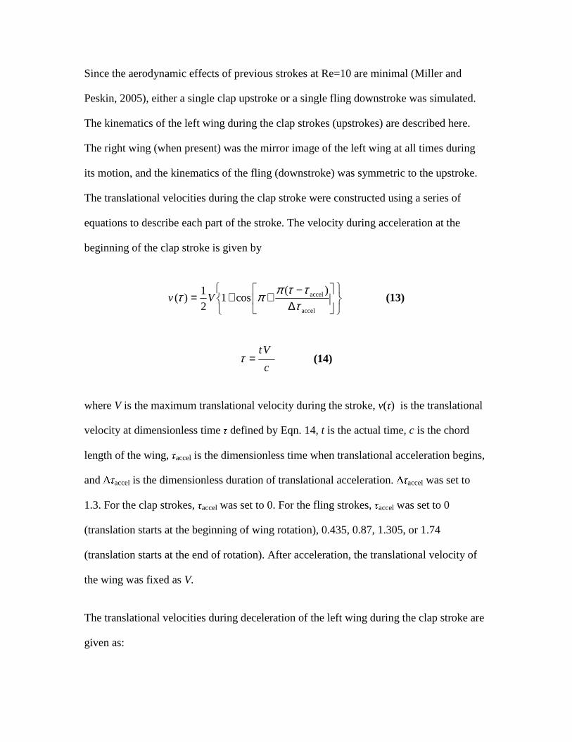
The translational velocities during the clap stroke were constructed using a series of

equations to describe each part of the stroke. The velocity during acceleration at the

beginning of the clap stroke is given by

(13) )(

cos12

1)(

accel

accel

∆−

++=τ

ττππτ Vv

(14) c

Vt=τ

where V is the maximum translational velocity during the stroke, v(τ ) is the translational

velocity at dimensionless time τ defined by Eqn. 14, t is the actual time, c is the chord

length of the wing, τaccel is the dimensionless time when translational acceleration begins,

and � τaccel is the dimensionless duration of translational acceleration. � τ

accel was set to

1.3. For the clap strokes, τaccel was set to 0. For the fling strokes, τ

accel was set to 0

(translation starts at the beginning of wing rotation), 0.435, 0.87, 1.305, or 1.74

(translation starts at the end of rotation). After acceleration, the translational velocity of

the wing was fixed as V.

The translational velocities during deceleration of the left wing during the clap stroke are

given as:

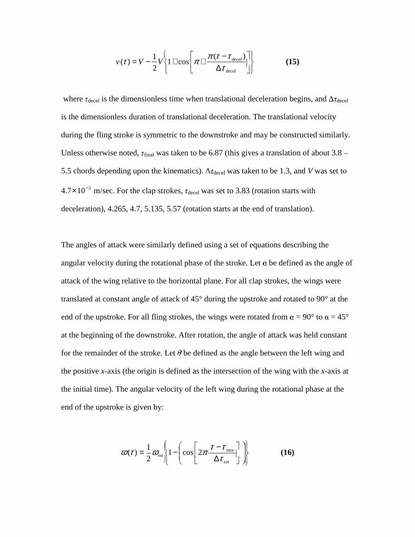
(15) )(

cos12

1)(

decel

decel

∆−

++−=τ

ττππτ VVv

where τdecel is the dimensionless time when translational deceleration begins, and � τ

decel

is the dimensionless duration of translational deceleration. The translational velocity

during the fling stroke is symmetric to the downstroke and may be constructed similarly.

Unless otherwise noted, τfinal was taken to be 6.87 (this gives a translation of about 3.8 –

5.5 chords depending upon the kinematics). � τdecel was taken to be 1.3, and V was set to

4.7 310−× m/sec. For the clap strokes, τdecel was set to 3.83 (rotation starts with

deceleration), 4.265, 4.7, 5.135, 5.57 (rotation starts at the end of translation).

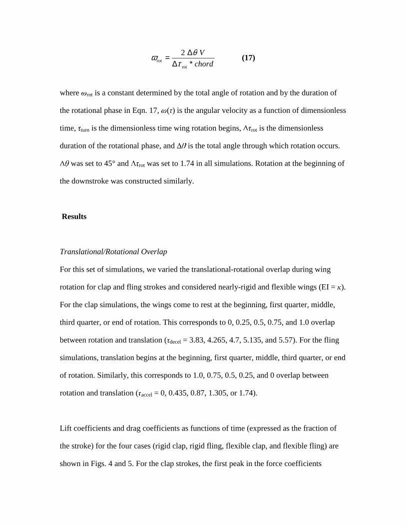
The angles of attack were similarly defined using a set of equations describing the

angular velocity during the rotational phase of the stroke. Let α be defined as the angle of

attack of the wing relative to the horizontal plane. For all clap strokes, the wings were

translated at constant angle of attack of 45° during the upstroke and rotated to 90° at the

end of the upstroke. For all fling strokes, the wings were rotated from α = 90° to α = 45°

at the beginning of the downstroke. After rotation, the angle of attack was held constant

for the remainder of the stroke. Let θ be defined as the angle between the left wing and

the positive x-axis (the origin is defined as the intersection of the wing with the x-axis at

the initial time). The angular velocity of the left wing during the rotational phase at the

end of the upstroke is given by:

(16) 2cos12

1)(

rot

turnrot

∆−

−=τττπωτω

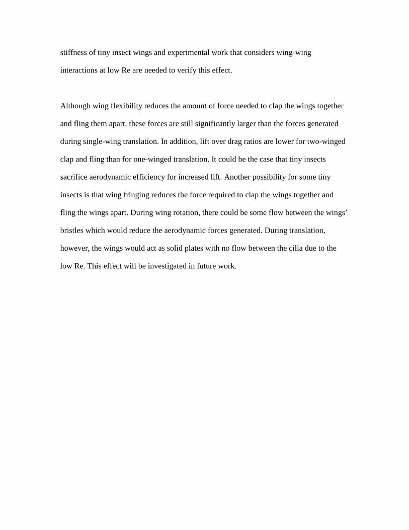
(17) 2

rotrot chord

V

∗∆∆=

τθω

where ω rot is a constant determined by the total angle of rotation and by the duration of

the rotational phase in Eqn. 17, ω (τ ) is the angular velocity as a function of dimensionless

time, τturn is the dimensionless time wing rotation begins, � τ

rot is the dimensionless

duration of the rotational phase, and � θ is the total angle through which rotation occurs. � θ

was set to 45° and � τrot was set to 1.74 in all simulations. Rotation at the beginning of

the downstroke was constructed similarly.

Results

Translational/Rotational Overlap

For this set of simulations, we varied the translational-rotational overlap during wing

rotation for clap and fling strokes and considered nearly-rigid and flexible wings (EI = κ ).

For the clap simulations, the wings come to rest at the beginning, first quarter, middle,

third quarter, or end of rotation. This corresponds to 0, 0.25, 0.5, 0.75, and 1.0 overlap

between rotation and translation (τdecel = 3.83, 4.265, 4.7, 5.135, and 5.57). For the fling

simulations, translation begins at the beginning, first quarter, middle, third quarter, or end

of rotation. Similarly, this corresponds to 1.0, 0.75, 0.5, 0.25, and 0 overlap between

rotation and translation (τaccel = 0, 0.435, 0.87, 1.305, or 1.74).

Lift coefficients and drag coefficients as functions of time (expressed as the fraction of

the stroke) for the four cases (rigid clap, rigid fling, flexible clap, and flexible fling) are

shown in Figs. 4 and 5. For the clap strokes, the first peak in the force coefficients

corresponds to the acceleration of the wing from rest. The force coefficients quickly

reach steady values until the wings begin to decelerate and rotate. The next peak in the

force coefficients corresponds to the rotation of the wings together (clap). Large lift and

drag forces are produced as the air between the wings is squeezed downward. Note that

lift coefficients produced during the rigid and flexible clap strokes are comparable, but

the drag coefficients produced during the clap are significantly lower in the flexible case.

For the fling strokes, the first peak in the force coefficients corresponds to the rotation of

the wings apart (fling). The peak lift forces in the flexible cases are higher than the

corresponding rigid cases. There are a couple of possible explanations for this

phenomenon. Peel delays the formation of the trailing edge vortices, thereby maintaining

vortical asymmetry and augmenting lift for longer periods (Miller and Peskin, 2005).

Similarly, the suppression of the formation of the trailing edge vortex would also reduce

the Wagner effect at the beginning of translation (Weis-Fogh, 1973). Lift augmentation

by ‘peel’ verses ‘fling’ was also predicted using simple analytic models of inviscid flows

around rigid wings (Ellington, 1984). As the wings are peeled apart, the wings are

deformed and store elastic energy. As the wings translate apart, the wings ‘straighten’

and push down on the fluid, causing an upwards lift force. Furthermore, the peak drag

forces produced during fling are significantly lower in the flexible cases than in the rigid

cases. As a result of the peel, the time rate of change of the volume between the wings is

reduced relative to the rigid wing case.

For a comparison of the average forces generated in each case, lift and drag coefficients

were averaged over wing rotation and 2.5 chord lengths of travel as shown in Fig. 6. For

the fling cases, average lift coefficients increase as the amount of rotational/translational

overlap increases. In the case of 100% overlap, average lift forces are larger in the

flexible case than in the rigid case. For other degrees of overlap, average lift coefficients

for rigid and flexible wings are comparable. For all overlap fling cases, the average drag

coefficients produced by flexible wings are lower than those produced by rigid wings.

Moreover, the average lift over drag force produced during fling is higher for flexible

wings than for rigid wings. This effect increases as the degree of rotational/translational

overlap is increased. For the clap cases, average lift coefficients are comparable for rigid

and flexible wings, and these forces increase as the degree of rotational/translational

overlap increases. The average drag forces produced in the rigid wing cases, however, are

higher than the corresponding flexible wing cases. As a result, average lift over drag is

higher for flexible wings. In summary, these results suggest that wing flexibility could

improve the efficiency of hovering flight at low Re.

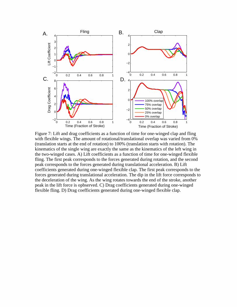
One-winged simulations with flexible wings were performed using the same kinematics

as in the two-winged cases, and the force coefficients as functions of time are shown in

Fig. 7. During the fling motion, the first peak in the force coefficients corresponds to the

forces generated during rotation, and the second peak corresponds to the forces generated

during translational acceleration. Wing deformation during one-winged clap and fling is

minimal, and these force traces are similar to the rigid wing case. During the clap motion,

the first peak in the force coefficients corresponds to the forces generated during

translational acceleration. The first dip in the force coefficients towards the end of the

stroke corresponds to the deceleration of the wing. As the wing rotates towards the end of

the stroke, another peak in the lift and drag forces force is observed. These forces quickly

drop as the wing decelerates to rest. Force coefficients for one-winged clap and fling

averaged over rotation and 2.5 chord lengths of translation are shown in Fig. 8.

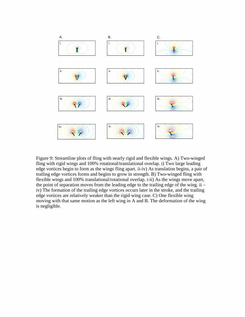
Streamline plots of the fluid flow around wings performing a fling with 100% overlap

between the translational and rotational phases are shown in Fig. 9. Two-winged fling

with rigid wings is shown in Fig. 9A. During wing rotation, two large leading edge

vortices begin to form as the wings fling apart (i-ii). As translation begins, a pair of

trailing edge vortices forms and begins to grow in strength (ii – iv). Two-winged fling

with flexible wings (EI = κ ) is shown in Fig. 9B. The wings move with the same motion

as in 9A (100% rotational/translational overlap). As the wings move apart, the point of

separation moves from the leading edge to the trailing edge of the wing (i-ii). The

formation of the trailing edge vortices occurs later in the stroke, and the trailing edge

vortices are relatively weaker than the rigid wing case (ii–iv). One flexible wing (EI = κ )

moving with the same fling motion as A and B is shown in Fig. 9C. Due to the smaller

aerodynamic forces acting on the wing, its deformation is negligible.

Streamline plots of the flow around wings performing a clap with 100% overlap between

the translational and rotational phases are shown in Fig. 10. Two-winged clap with rigid

wings is shown in 10A. As the wings clap together, the fluid is pushed out between the

trailing edges causing an upwards lift force (i-iv). Two-winged clap with flexible wings

(EI = κ ) using the same motion is shown in 10B. Towards the end of the stroke, the wings

bend as they are clapped together, reducing the peak drag forces generated (ii-iv). In

addition, the point of ‘attachment’ moves from the leading edge to the trailing edge of the

wing. One flexible wing (EI = κ ) moving with the same clap motion is shown in 10C.

Due to the smaller aerodynamic forces acting on the wing, its deformation is negligible.

Varying wing flexibilities

In this set of simulations, the flexural stiffness of the wings was varied from 0.25 κ to 2 κ ,

and the translational/rotational during clap and fling overlap was set to 100%. The lift

and drag coefficients for clap and fling cases are shown in Fig 11. Lift coefficients as

functions of dimensionless time during two-winged flexible fling are shown in 11A. The

largest lift forces are produced for the case where EI = 1.25κ . Lift coefficients decrease as

the bending stiffness of the wing increases or decreases from this value. Lift coefficients

generated during two-winged flexible clap are shown in 11B. The lift coefficients are

comparable for all five values of the bending stiffness. Drag coefficients generated during

two-winged flexible fling are shown in 11C. For this range of values, the drag

coefficients increase with increasing bending stiffness. Drag coefficients generated

during two-winged flexible clap are shown in 11D. Drag coefficients also increase with

increasing bending stiffness for this range of values.

Average lift and drag coefficients during wing rotation and a 2.5 chord translation are

shown in Fig. 12. Average lift coefficients for flexible clap and fling are shown in Fig.

12A. The average lift coefficient generated during fling was greatest when the bending

stiffness was set to 1.25 κ . The average lift generated during clap was relatively constant

for this range of values. The average drag coefficients for flexible clap and fling are

shown in 12B. For the both clap and fling, the average drag coefficients increase with

increasing bending stiffness. Average lift over drag ratios for flexible clap and fling are

shown in 12C. Lift over drag increases with decreasing bending stiffness.

Varying the rigid section of the wing

To investigate the affect of wing stiffness asymmetries on the forces produced during

flight, the rigid section of the flexible wing (1/5 of the chord length) was moved from the

leading to the trailing edge of the wing in five steps. In all cases, the flexural stiffness of

the wings was set to 1.0κ . The rotational/translational overlap was set to 100%. Combes

and Daniels (2003) measured the flexural stiffness of Manduca sexta wings as a function

of distance along the chord and found that the bending stiffness decreases from the

leading to the trailing edge of the wing. A quick look at the wing morphology of most

insect wings suggests that this is true for many species, making the assumption that

flexural stiffness is proportional to wing thickness. There might be a few exceptions to

this rule, however. For example, if the bristles of thrips’ wings are more flexible than the

solid portion, then there may be some variation in the location of the stiffest portion of

the wing as a function of distance from the leading to the trailing edge (see Fig. 13).

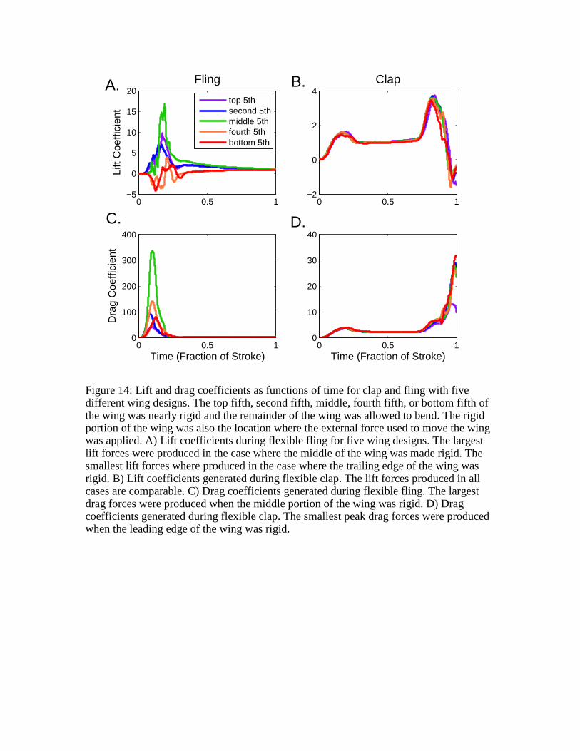
Lift coefficients and drag coefficients as functions of time (expressed as the fraction of

the stroke) for clap and fling with the various wing designs are shown in Fig. 14. In all

cases, the rotational/translational overlap was set to 100% and the flexural stiffness of the

wing was set to EI = κ . The rigid portion of the wing was also the location where the

external force used to move the wing was applied. Lift coefficients during flexible fling

are shown in 14A. The largest lift forces were produced in the case where the middle of

the wing was made rigid. The smallest lift forces where produced in the case where the

trailing edge of the wing was rigid. Lift coefficients generated during flexible clap are

shown in 14B. The lift forces produced for all wing designs are comparable. Drag

coefficients generated during flexible fling are shown in 14C. The largest drag forces

were produced when the middle portion of the wing was rigid. These forces are

significantly larger than all other cases. Drag coefficients generated during flexible clap

are shown in 14D. The smallest peak drag forces were produced when the leading edge of

the wing was rigid.

Average lift and drag coefficients during rotation and a 2.5 chord translation are shown in

Fig. 15. Average lift coefficients as a function of the wing design (location of the rigid

portion of the wing) for flexible clap and fling are shown in 15A.The average lift

coefficient generated during fling was greatest when the middle part of the wing was

rigid. The lowest lift forces were generated when the trailing edge of the wing was rigid.

The average lift generated during clap was relatively constant for each wing design.

Average drag coefficients are shown in 15B. In the case of fling, the largest average drag

coefficients were generated when the middle part of the wing was rigid. These forces

dropped as the rigid part was moved to either the leading or trailing edge of the wing. In

the case of clap, the forces generated were relatively constant. Average lift over drag for

clap and fling as a function of the location of the rigid part of the wing are shown in 15C.

Average lift over drag increases as the rigid part is moved towards the leading edge of the

wing.

Streamline plots of the flow around wings during fling for three wing designs are shown

in Fig 16. The flow around two wings designed so that the rigid part of the wing is along

the leading edge is shown in 16A. Two large leading edge vortices begin to form as the

wings fling apart (i-ii). As translation begins, a pair of trailing edge vortices forms and

begins to grow in strength (ii–iv). The flow around two wings where the rigid part is in

the middle of the wing is shown in 16B. As the wings are pulled apart, large deformations

of the wings occur along the leading and trailing edges (i-ii). When the leading and

trailing edges separate, large leading edge vortices are formed (ii-iv). The flow around

two wings where the rigid part of the wing is along the trailing edge is shown in 16C. As

the wings move apart, the point of separation moves from the trailing to the leading edge

of the wing. Large trailing edge vortices are formed at the beginning of the stroke.

Streamline plots of the flow around wings performing clap with three different wing

designs are shown in Fig. 17. Flow around two wings where the rigid part of the wing is

along the leading edge is shown in 17A. Towards the end of the stroke, the wings bend as

they are clapped together, reducing the peak drag generated. Flow around two wings

where the rigid part of the wing is in the middle of the wing is shown in 17B. This case is

similar to the rigid wing case since wing deformations are minimal. Flow around two

wings where the rigid part of the wing is at the trailing edge is shown in 17C. This case is

also similar to the rigid wing case since wing deformations are minimal.

Discussion

The results of this study suggest that wing flexibility is important for reducing drag and

increasing lift forces generated during clap and fling at low Reynolds numbers. For

flexible wings, the fling part of the stroke is more like a peel, and the clap part of the

stroke is more like a reverse peel. When wing translation begins with wing rotation

(100% overlap), lift forces are significantly higher for flexible wings. As the wings peel

apart, the point of separation travels from the leading to the trailing edge of the wing.

This delays the formation of the trailing edge vortices, which reduces the Wagner effect

and sustains vortical asymmetry (large leading edge vortex and small trailing edge

vortex) for a larger portion of the stroke. Increased lift production by wing peel vs. fling

was also predicted by Ellington (1984).

Asymmetries in flexural stiffness along the wing chord also influence aerodynamic

performance. Wings that are more rigid along the trailing edge of the wing maximize the

average lift/drag forces produced during fling. Wings that are more rigid in the middle

maximize the average lift force produced during fling. This result suggests that

differences in wing design could reflect different performance parameters that an insect

has ‘maximized.’

Average lift forces were greatest during fling when the flexural stiffness of the wing was

set to EI = 1.25κ . Using this value for the flexural stiffness of the wings, deformations

during translation or single wing flapping are minimal, and the force coefficients

produced are comparable to the rigid wing case. These results agree with the qualitative

observations of Ellington (1984) who oscillated single thrips’ wings at the frequency and

amplitude characteristic of flight. Since the forces generated during the clap and fling

portion of the strokes are so much larger than the single wing case due to wing-wing

interactions, wing deformations in the numerical simulations presented in this paper are

significant and greatly influence the aerodynamics. Measurements of the actual flexural

stiffness of tiny insect wings and experimental work that considers wing-wing

interactions at low Re are needed to verify this effect.

Although wing flexibility reduces the amount of force needed to clap the wings together

and fling them apart, these forces are still significantly larger than the forces generated

during single-wing translation. In addition, lift over drag ratios are lower for two-winged

clap and fling than for one-winged translation. It could be the case that tiny insects

sacrifice aerodynamic efficiency for increased lift. Another possibility for some tiny

insects is that wing fringing reduces the force required to clap the wings together and

fling the wings apart. During wing rotation, there could be some flow between the wings’

bristles which would reduce the aerodynamic forces generated. During translation,

however, the wings would act as solid plates with no flow between the cilia due to the

low Re. This effect will be investigated in future work.

References

ALBEN, S., SHELLEY, M., AND ZHANG, J. (2002). Drag reduction through self-

similar bending of a flexible body. Nature. 420, 479-481.

ALBEN, S., SHELLEY, M., AND ZHANG, J. How flexibility induces streamlining in a

two-dimensional flow. To appear Physics of Fluids, 2004.

CHILDRESS, S. AND DUDLEY, R. Transition from ciliary to flapping mode in a

swimming mollusc: Flapping flight as a bifurcation in Re_omegsa. In publication,

J. Fluid Mech.

CLOUPEAU, M., DEVILLERS, J. F. AND DEVEZEAUX, D. (1979). Direct

measurements of instantaneous lift in desert locust: comparison with Jensen’s

experiments on detached wings. J. exp. Biol. 80, 1-15.

DENNY, M. (1994). Extreme drag forces and the survival of wind-swept and water-

swept organisms. J. Exp. Biol. 194, 97-115.

DICKINSON, M. H. (1994). The effects of wing rotation on unsteady aerodynamic

performance at low Reynolds numbers. J. exp. Biol. 192, 179-206.

DICKINSON, M. H. and GÖTZ, K. G. (1993). Unsteady aerodynamic performance of

model wings at low Reynolds numbers. J. exp. Biol. 174, 174.

DICKINSON, M. H. and GÖTZ, K. G. (1996). The wake dynamics and flight forces of

the fruit fly Drosophila melanogaster. J. exp. Biol. 199, 2085-2104.

DICKINSON, M. H., Lehmann, F. -O., and Sane, S. P. (1999). Wing rotation and the

aerodynamic basis of insect flight. Science 284, 1954-1960.

DUDLEY, R. (2000). The biomechanics of insect flight: form, function, evolution.

Princeton: Princeton University Press.

ELLINGTON, C. P. (1984b). The aerodynamics of hovering insect flight. III.

Kinematics. Phil. Trans. R. Soc. Lond. B 305, 41-78.

ELLINGTON, C. P. (1999). The novel aerodynamics of insect flight: Applications to

micro-air vehicles. J. exp. Biol. 202, 3439–3448.

ETNIER, S. A. AND VOGEL, S. (2000). Reorientation of daffodil (Narcissus:

Amaryllidaceae) flowers in wind: Drag reduction and torsional flexibility. Am. J.

Bot. 87(1), 29-32.

FAUCI, L. J. (1990). Interaction of oscillating filaments – A computational study. J.

Comput. Phys., 86, 294.

FAUCI, L. J. AND FOGELSON, A. L. (1993). Truncated Newton methods and the

modeling of complex elastic structures. Comm. Pure Appl. Math., 46, 787.

FAUCI, L. J. AND PESKIN, C. S. A computational model of aquatic animal locomotion.

J. Comput. Phys. 77, 85.

GRUNBAUM, D. EYRE, D. AND FOGELSON, A. (1998). Functional geometry of

ciliated tentacular arrays in active suspension feeders. J. Exp. Biol., 201, 2575-

2589.

HAUSSLING, H. J. (1979). Boundary fitted coordinates for accurate numerical solution

of multibody flow problems. J. Comp. Phys. 30, 107 – 124.

HORRIDGE, G. A. (1956). The flight of very small insects. Nature 178, 1334-1335.

KIM, Y. AND PESKIN, C. S. 2-D Parachute Simulation by the Immersed Boundary

Method. Submitted to SIAM Journal on Scientific Computing.

KOEHL, M. A. R. (1984). How do benthic organisms withstand moving water? Am.

Zool. 24, 57-70.

KOEHL, M. A. R. (1995). Fluid flow through hair-bearing appendages: Feeding,

smelling, and swimming at low and intermediate Reynolds number. In C.P.

Ellington and T. J. Pedley [eds.], Biological Fluid Dynamics, Soc. Exp. Biol.

Symp. 49, 157-182.

LAI, M. -C. AND PESKIN (2000). An immersed boundary method with formal second

order accuracy and reduced numerical viscosity. Journal of Computational

Physics 160, 705-719.

LEHMANN, F.-O., SANE, S. P., and DICKINSON, M. (2005). The aerodynamic effects

of wing-wing interaction in flapping insect wings. J. Exp. Biol., 208(16), 3075 -

3092.

LIGHTHILL, M. J. (1973). On the Weis-Fogh mechanism of lift generation. J. Fluid

Mech. 60, 1-17.

MAXWORTHY, T. (1979). Experiments on the Weis-Fogh mechanism of lift generation

by insects in hovering flight. Part I. Dynamics of the ‘fling.’ J. Fluid Mech. 93,

47-63.

MC QUEEN, M. C. AND PESKIN, C. S. (2000). A three-dimensional computer model

of the human heart for studying cardiac fluid dynamics. Computer Graphics. 34,

56.

MILLER, L. A. and PESKIN, C. S. (2005). A computational fluid dynamics of `clap and

fling' in the smallest insects. J. Exp. Biol., 208(2): 195 - 212.

LEHMANN, F. –O., SANE, S. P. AND DICKINSON, M. (2005). The aerodynamic

effects of wing–wing interaction in flapping insect wings

J. Exp. Biol. 208, 3075-3092.

OSBORNE, M. F. M. (1951). Aerodynamics of flapping flight with application to

insects. J. Exp. Biol. 28, 221-245.

PESKIN, C. S. (2002). The immersed boundary method. Acta Numerica, 11, 479-517.

PESKIN, C. S. (1977). Flow patterns around heart valves: A numerical method. J.

Comput. Phys. 25, 220.

PESKIN, C. S. AND MCQUEEN, D. M. (1996). Fluid dynamics of the heart and its

valves. In Case studies in mathematical modeling – Ecology, physiology, and cell

biology, (Othmer, H. G., Adler, F. R., Lewis, M. A. and Dallon, J. C.), pp. 309-

337. New Jersey: Prentice Hall, Inc.

SANE, S. P. AND DICKINSON, M. H. (2002). The aerodynamic effects of wing rotation

and a revised quasi-steady model of flapping flight. J. exp. Biol. 205, 1087-1096.

SPEDDING, G. R. AND MAXWORTHY, T. (1986). The generation of circulation and

lift in a rigid two-dimensional fling. J. Fluid Mech. 165, 247-272.

SUN, M. AND TANG, J. (2002). Unsteady aerodynamic force generation by a model

fruit fly wing in flapping motion. J. exp. Biol. 205, 55-70.

SUN, M. AND XIN, Y. (2003). Flow around two airfoils performing fling and

subsequent translation and translation and subsequent flap. Acta Mechanica

Sinica 19, 103-117.

SUNADA, S., KAWACHI, K., WATANABE, I., AND AZUMA, A. (1993).

Fundamental Analysis of three-dimensional ‘near fling.’ J. Exp. Biol. 183, 217-

248.

SUNADA, S., TAKASHIMA, H., HATTORI, T., YASUDA, K., AND KAWACHI, K.

(2002). Fluid-dynamic characteristics of a bristled wing. J. Exp. Biol. 205, 2737-

2744.

VANDENBERGHE, N., ZHANG, J. AND CHILDRESS, S. (2004). Symmetry breaking

leads to forward flapping flight. To appear J. of Fluid Mechanics.

VOGEL, S. (1989). Drag and reconfiguration of broad leaves in high winds. J. Exp. Bot.

40, 941-948.

WEIS-FOGH, T. (1973). Quick estimates of flight fitness in hovering animals, including

novel mechanisms for lift production. J. exp. Biol. 59, 169-230.

WU, J. C. (1981). Theory for aerodynamic force and moment in viscous flows. AIAA J.

19, 432-441.

ZANKER, J. M. AND GÖTZ, K. G. (1990). The wing beat of Drosophila melanogaster.

II. Dynamics. Phil. Trans. R. Soc. Lond. B 327, 19-44.

Figure 1: The peel mechanism of lift generation in insect flight, redrawn from Ellington (1984). A) A two-dimensional diagram of the circulation around two wings performing a peel. B) A rigid model of ‘flat peel.’

Β represents half of the angle between the wings, x

represents the exposed portion of the wing, and u represents the velocity of the separation point. C) The circulation function f(β ).

Figure 2: The clap mechanism of lift generation in insect flight, redrawn from Ellington (1984). A) A two-dimensional diagram of the circulation around two wings performing a clap. The clap motion creates a jet of air downward. B) A two dimensional diagram of flexible clap or reverse peel. As the wings are clapped together, the point of attachment moves from the leading to the trailing edge of the wing.

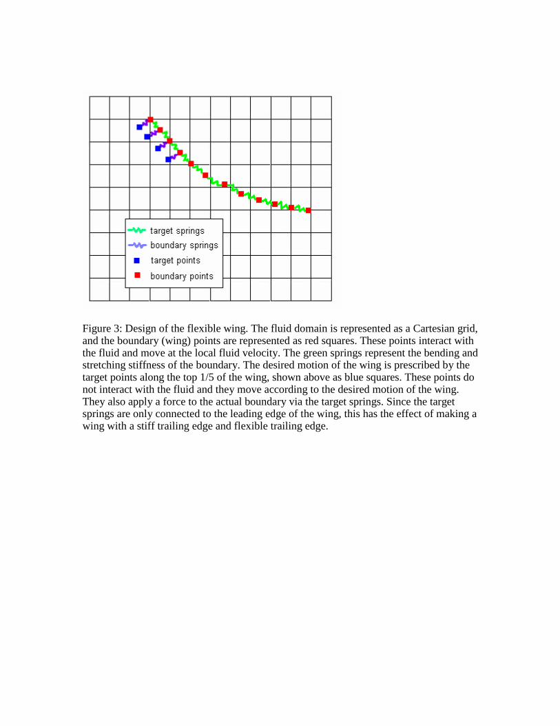
Figure 3: Design of the flexible wing. The fluid domain is represented as a Cartesian grid, and the boundary (wing) points are represented as red squares. These points interact with the fluid and move at the local fluid velocity. The green springs represent the bending and stretching stiffness of the boundary. The desired motion of the wing is prescribed by the target points along the top 1/5 of the wing, shown above as blue squares. These points do not interact with the fluid and they move according to the desired motion of the wing. They also apply a force to the actual boundary via the target springs. Since the target springs are only connected to the leading edge of the wing, this has the effect of making a wing with a stiff trailing edge and flexible trailing edge.

0 0.2 0.4 0.6 0.8 1−2

0

2

4

6

8

10

Lift

Coe

ffici

ent

Rigid

Lift

Coe

ffici

ent

0 0.2 0.4 0.6 0.8 1−2

0

2

4

6

8

10Flexible

0 0.2 0.4 0.6 0.8 1−2

−1

0

1

2

3

4

0 0.2 0.4 0.6 0.8 1−2

−1

0

1

2

3

4

Time (Fraction of Stroke)Time (Fraction of Stroke)

100% overlap75% overlap50% overlap25% overlap0% overlap

A. B.

C. D.

Figure 4: Lift coefficients as functions of time for flexible and rigid clap and fling. A) Fling with rigid wings for 0%, 25%, 50%, 75%, and 100% overlap between the rotational and translational phases of the stroke. The first peak occurs during wing rotation, and the second peak occurs during translational acceleration. The largest lift forces are generated when rotation and translation begin at the beginning of the stroke (100% overlap). B) Fling with flexible wings. Larger peak lift forces are produced due to the peel mechanism (see results) and elastic storage. C) Clap with rigid wings. The first peak in the lift force occurs during translational acceleration. The second peak occurs during wing rotation as the wings are clapped together. D) Clap with flexible wings. Lift forces generated during clap flexible wings are very similar to the forces generated with rigid wings.

0 0.2 0.4 0.6 0.8 10

20

40

60

80

100

Dra

g C

oeffi

cien

t

Rigid

Dra

g C

oeffi

cien

t

0 0.2 0.4 0.6 0.8 10

20

40

60

80

100Flexible

0 0.2 0.4 0.6 0.8 1

0

20

40

60

80

Time (Fraction of Stroke)Time (Fraction of Stroke)Time (Fraction of Stroke) Time (Fraction of Stroke)0 0.2 0.4 0.6 0.8 1

0

20

40

60

80

100% overlap75% overlap50% overlap25% overlap0% overlap

A. B.

C. D.

Figure 5: Drag coefficients as functions of time for flexible and rigid clap and fling. A) Fling with rigid wings for 0%, 25%, 50%, 75%, and 100% overlap between the rotational and translational phases of the stroke. A very large peak in the drag force occurs during wing rotation as the wings are pulled apart. The largest drag forces are generated when rotation and translation begin at the beginning of the stroke (100% overlap). B) Fling with flexible wings. The peak drag forces produced are significantly lower in the flexible wing case. C) Clap with rigid wings. A large peak in the drag force occurs towards the end of the stroke as the wings are clapped together. D) Clap with flexible wings. Peak drag forces generated during clap with flexible wings are significantly lower than those generated by rigid wings.

0 0.5 10

0.5

1

1.5

2

Ave

rage

CL

0 0.5 10

2

4

6

8

10

Rotational/Translational Overlap

Ave

rage

CD

0 0.5 10

0.1

0.2

0.3

0.4

Ave

rage

CL /

CD

0 0.5 10

1

2

3

Ave

rage

CL

0 0.5 10

5

10

15

20

Rotational/Translational Overlap

Ave

rage

CD

0 0.5 10

0.1

0.2

Ave

rage

CL /

CD

FlexibleRigid

A. B. C.

D. E. F.

Figure 6: Average lift and drag coefficients generated during wing rotation and a translation of 2.5 chord lengths in the case of fling (top) and clap (bottom). A) Average lift coefficients during fling increase as the amount of rotational/translational overlap increases. In the case of 100% overlap, average lift forces are larger in the flexible case. In the other cases, average lift coefficients in the rigid and flexible cases are comparable. B) In all cases, the average drag forces produced by flexible wings are lower than those produced by rigid wings. C) In all cases, the average lift over drag produced is higher for flexible wings. This effect increases as the degree of rotational/translational overlap is increased. D) Average lift coefficients produced during clap are comparable for the rigid and flexible cases, and these forces increase as the degree of rotational/translational overlap increases. E) The average drag forces produced in the rigid wing cases are higher than the corresponding flexible wing cases. F) Average lift over drag is higher in the flexible wing cases.

0 0.2 0.4 0.6 0.8 1−2

−1

0

1

2

3

4

Lift

Coe

ffici

ent

Fling

0 0.2 0.4 0.6 0.8 1−4

−2

0

2

4Clap

0 0.2 0.4 0.6 0.8 1−2

0

2

4

6

8

Time (Fraction of Stroke)

Dra

g C

oeffi

cien

t

Time (Fraction of Stroke)0 0.2 0.4 0.6 0.8 1

−4

−2

0

2

4

100% overlap75% overlap50% overlap25% overlap0% overlap

A. B.

C. D.

Figure 7: Lift and drag coefficients as a function of time for one-winged clap and fling with flexible wings. The amount of rotational/translational overlap was varied from 0% (translation starts at the end of rotation) to 100% (translation starts with rotation). The kinematics of the single wing are exactly the same as the kinematics of the left wing in the two-winged cases. A) Lift coefficients as a function of time for one-winged flexible fling. The first peak corresponds to the forces generated during rotation, and the second peak corresponds to the forces generated during translational acceleration. B) Lift coefficients generated during one-winged flexible clap. The first peak corresponds to the forces generated during translational acceleration. The dip in the lift force corresponds to the deceleration of the wing. As the wing rotates towards the end of the stroke, another peak in the lift force is opbserved. C) Drag coefficients generated during one-winged flexible fling. D) Drag coefficients generated during one-winged flexible clap.

0 0.5 10

0.5

1

1.5

Ave

rage

CL

0 0.5 10

0.5

1

1.5

2

2.5

Rotational/Translational Overlap

Ave

rage

CD

0 0.5 10

0.5

1

1.5

Ave

rage

CL /

CD

FlingClap

A. B. C.

Figure 8: Average lift and drag coefficients for one-winged flexible clap and fling. The rotational/translational overlap was set to 0%, 25%, 50%, 75%, and 100%. Force coefficients were averaged over rotation and a 2.5 chord length translation. A) Average lift coefficients increase during the fling motion as the degree of rotational/translational overlap increases. However, average lift coefficients during clap decrease slightly as the amount of rotational/translational overlap increases. B) A similar pattern is seen for the drag forces generated during one-winged clap and fling. C) The average lift over drag forces produced during one-winged clap and fling remain relatively constant as the degree of rotational/translational overlap is varied.

A. B. C.

i. i. i.

ii. ii. ii.

iii. iii. iii.

iv. iv. iv.

Figure 9: Streamline plots of fling with nearly rigid and flexible wings. A) Two-winged fling with rigid wings and 100% rotational/translational overlap. i) Two large leading edge vortices begin to form as the wings fling apart. ii-iv) As translation begins, a pair of trailing edge vortices forms and begins to grow in strength. B) Two-winged fling with flexible wings and 100% translational/rotational overlap. i-ii) As the wings move apart, the point of separation moves from the leading edge to the trailing edge of the wing. ii – iv) The formation of the trailing edge vortices occurs later in the stroke, and the trailing edge vortices are relatively weaker than the rigid wing case. C) One flexible wing moving with that same motion as the left wing in A and B. The deformation of the wing is negligible.

A. B. C.

i. i. i.

ii. ii. ii.

iii. iii. iii.

iv. iv. iv.

Figure 10: Streamline plots of clap with nearly rigid and flexible wings. A) Two-winged clap with rigid wings and 100% rotational/translational overlap. i-iv) As the wings clap together, the fluid is pushed out between the trailing edges. B) Two-winged clap with flexible wings and 100% translational/rotational overlap. ii-iv) Towards the end of the stroke, the wings bend as they are clapped together, reducing the peak drag generated. As the wings move together, the point of ‘attachment’ moves from the leading edge to the trailing edge of the wing. C) One flexible wing moving with that same motion as the left wing in A and B. The deformation of the wing is negligible.

0 0.5 1−2

0

2

4

6

8

10

Lift

Coe

ffici

ent

Fling

0 0.5 1−2

0

2

4

6

8

10Clap

0 0.5 10

20

40

60

Time (Fraction of Stroke)

Dra

g C

oeffi

cien

t

0 0.5 10

5

10

15

20

Time (Fraction of Stroke)

EI = 2κEI = 1.5κEI = 1.0κEI = 0.5κEI = 0.25κ

A. B.

C. D.

Figure 11: Lift and drag coefficients as functions of time for flexible clap and fling with 100% rotational/translational overlap and for five bending coefficients. A) Lift coefficients generated during two-winged flexible fling. The largest average lift forces are produced for the case where EI = 1.0κ . B) Lift coefficients generated during two-winged flexible clap. The lift coefficients are comparable for all five cases. C) Drag coefficients generated during two-winged flexible fling. The peak drag forces generated increase with increasing bending stiffness. D) Drag coefficients generated during two-winged flexible clap. Peak drag forces increase with increasing bending stiffness.

0 1 20

0.5

1

1.5

2

2.5

Ave

rage

CL

0 1 20

2

4

6

8

10

Flexural Stiffness

Ave

rage

CD

0 1 20

0.1

0.2

0.3

0.4

0.5

Ave

rage

CL /

CD

ClapFling

A. B. C.

Figure 12: Average lift and drag coefficients during rotation and a 2.5 chord translation as a function of the bending stiffness. The bending stiffness was set to 0.25κ , 0.5κ , 0.75κ , 1.0κ , 1.25κ , 1.5κ , and 2.0κ . A) The average lift coefficient generated during fling was greatest when the bending stiffness was set to 1.25 κ . The average lift generated during clap was relatively constant for this range of bending stiffness. B) For the both cases, the average drag coefficients increase with increasing bending stiffness. C) Average lift over drag decreases with increasing bending stiffness.

[Insert picture of different types of thrips wings.] Figure 13:

0 0.5 1−5

0

5

10

15

20

Lift

Coe

ffici

ent

Fling

0 0.5 1−2

0

2

4Clap

0 0.5 10

100

200

300

400

Time (Fraction of Stroke)

Dra

g C

oeffi

cien

t

0 0.5 10

10

20

30

40

Time (Fraction of Stroke)

top 5thsecond 5thmiddle 5thfourth 5thbottom 5th

A. B.

C. D.

Figure 14: Lift and drag coefficients as functions of time for clap and fling with five different wing designs. The top fifth, second fifth, middle, fourth fifth, or bottom fifth of the wing was nearly rigid and the remainder of the wing was allowed to bend. The rigid portion of the wing was also the location where the external force used to move the wing was applied. A) Lift coefficients during flexible fling for five wing designs. The largest lift forces were produced in the case where the middle of the wing was made rigid. The smallest lift forces where produced in the case where the trailing edge of the wing was rigid. B) Lift coefficients generated during flexible clap. The lift forces produced in all cases are comparable. C) Drag coefficients generated during flexible fling. The largest drag forces were produced when the middle portion of the wing was rigid. D) Drag coefficients generated during flexible clap. The smallest peak drag forces were produced when the leading edge of the wing was rigid.

0 0.5 10

1

2

3

Ave

rage

CL

0 0.5 10

10

20

30

Rigid Part of Wing

Ave

rage

CD

0 0.5 10

0.1

0.2

0.3

0.4

Ave

rage

CL /

CD

ClapFling

A. B. C.

Figure 15: Average lift and drag coefficients during rotation and a 2.5 chord translation as a function of the portion of the wing that was made rigid. When the rigid part of the wing was set 0.2, the lower fifth (trailing edge) of the wing was rigid. When the rigid part of the wing was set to 1.0, the top fifth (leading edge) of the wing was rigid. A) The average lift coefficient generated during fling was greatest when the middle part of the wing was rigid. The lowest lift forces were generated when the trailing edge of the wing was rigid. The average lift generated during clap was relatively constant for each wing design. B) In the case of fling, the largest average drag coefficients were generated when the middle part of the wing was rigid. These forces dropped as the rigid part was moved to either the leading or trailing edge of the wing. In the case of clap, the forces generated were relatively constant. C) Average lift over drag increases as the rigid part is moved towards the leading edge of the wing.

A.

i. i. i.

ii. ii. ii.

iii. iii. iii.

iv. iv. iv.

B. C.

Figure 16: Streamline plots of fling with three different wing designs and 100% rotational/translational overlap. The flexible part of all wings was set to 1.0κ . A) The rigid part of the wing is along the leading edge. i) Two large leading edge vortices begin to form as the wings fling apart. ii-iv) As translation begins, a pair of trailing edge vortices forms and begins to grow in strength. B) The rigid part is in the middle of the wing. i-ii) As the wings are pulled apart, large deformations of the wings occur along the leading and trailing edges. iii – iv) When the leading and trailing edges separate, large leading edge vortices are formed. C) The rigid part of the wing is along the trailing edge. As the wings move apart, the point of separation moves from the trailing to the leading edge of the wing. Large trailing edge vortices are formed.