1

Ecosystem Profile Assessment of Biodiversity at

Loyola University Retreat and Ecology Campus

Summer 2014 Catherine Pacholski, Samantha Keyport, Joseph Gasior and Stephen Mitten

Institute of Environmental Sustainability

Loyola University Chicago

Abstract:

An ecosystem profile assessment of biodiversity for four plots representing four distinct terrestrial ecotypes and three small calcareous ponds within the 98-acre property of Loyola’s University Retreat and Ecology Campus (LUREC) were performed during June-mid August of 2014. Biodiversity testing protocols for the terrestrial ecosystems were based on those outlined in the “Ecosystem Profile Assessment of Biodiversity: Sampling Protocols and Procedures” of the U.S. Department of Interior and the National Park Service. Twenty biotic and abiotic protocols were selected. Species richness, Simpson Index of Diversity and the Shannon-Weiner’s Biodiversity Index were calculated for each ecotype. We found that, overall; the buckthorn and fen plots were more diverse than the oak hickory and shrubland plots. Seven biotic protocols and six abiotic protocols were performed on the three ponds. We found that the third pond, as expected, was the most diverse of all three ponds. The results serve as baseline data for studying the effects of climate change on ecosystems located in the Northern Illinois region as well as for monitoring ongoing restoration efforts on the campus.

Introduction:

A biodiversity assessment is a comprehensive analysis of an ecosystem including its

flora, fauna and abiotic factors. Certain aspects of biodiversity within LUREC have been

surveyed previously (plants by Dr. Roberta Lammers-Campbell, and Lepidoptera, birds, and

vertebrates by Edgar Perez and Stephen Mitten; see Perez and Mitten (2012) for birds), but an

overall property biodiversity analysis has not been completed. We conducted biodiversity

profiles, which include composition, structure, function, and inter-relationships of biotic and

abiotic components within a sample plot. We measured species richness and distribution of

organisms in order to determine their ecological roles at four defined sites. We then combined

this information with certain abiotic factors to create an overall ecosystem profile. The sampling

protocols, as developed by Mahan et al (1998), can be used to answer general research

questions. Our objectives in this project were to: 1) learn as much as possible about the main

ecosystems at LUREC; 2) collect data/samples and identify organisms present within the plots;

3) describe composition and inter-relationships between biotic and abiotic elements of each

habitat; 4) determine species richness and biodiversity of each ecosystem; 5) establish

standardized protocols for future surveying of the same or new ecosystems at LUREC; and 6)

promote future monitoring of these ecosystems. This research “provides a comprehensive

description of species assemblages and community structure within an ecosystem” (Mahan et

al.1998, p.10). LUREC’s biodiversity is important as it shows us what is currently here and thus

may also indicate the current health of each ecotype. We can then use this information in the

2

future as we monitor changes over time within each ecosystem type that was sampled on the

property so as to examine trends. The results can also serve as baseline data for studying the

effects of climate change on ecosystems located in the Northern Illinois region as well as for

monitoring ongoing restoration efforts on the campus.

Our assessment of the ecosystems began with a 20 x 20 m plot for each ecosystem.

The four main ecosystems studied include a successional shrubland, an oak-hickory woodland,

an invasive buckthorn-honeysuckle thicket, and a degraded calcareous fen. Often times, it is

nearly impossible to document an entire ecosystem due to time, size, and labor restraints. Thus,

sampling provides an adequate representation of an ecosystem’s relationships and processes

occurring on a larger scale. Since some species, like birds and bats, have larger, overlapping

habitats greater than a 20 x 20m plot, it is necessary to perform modified protocols to better

understand these species’ role in the entire ecosystem. We accounted for this difference with

supplemental mammal, herpetofaunal, and avian surveys.

A supplemental series of tests were conducted on the three small human constructed

retention ponds on the property. Since this is an aquatic environment, different sampling

protocols were conducted to obtain similar types of data as that of the terrestrial plots. We

wanted to: 1) understand what organisms are present in each pond; 2) observe differences and

changes of biotic and abiotic factors across each subsequent pond; 3) compare species

richness and biodiversity of each pond; 4) identify reasons for the differences and changes

across the ponds, if any; and 5) establish standardized protocols for future surveying of the

ponds. The data from this accompanying project will be found at the end of each section within

this paper.

Study Area:

LUREC is located at 2710 S. Country Club Road, Bull Valley, McHenry County, IL, and

encompasses 98 acres (9.7 hectares) total. The property is located in Section 13, Township 44,

North, Range 7, and East of the Third Meridian. LUREC, at its southeastern tip, is situated next

to the Parker Fen, an Illinois Nature Preserve (Perez and Mitten, 2012).

Various ecosystems exist within the property, including a buckthorn/honeysuckle invaded oak-

hickory woodland, a recreated prairie, a sedge meadow, a white pine grove, various shrub

lands, a calcareous fen, three small retention ponds, a small lake, and two stream ditches that

drain a wetland. Restoration efforts are currently under way in the prairie and the oak-hickory

woodland. On the eastern side of the property, natural forests and wetlands have been

overgrown by invasive buckthorn and honeysuckle. These invasive species have interrupted

many of natural ecosystem processes and have made travel through these areas difficult.

Restoration ecologists and volunteers have been working since January 2012 to remove these

invasive species and restore native vegetation. Travel through this area was possible via trails

created by past LUREC Interns and Restoration volunteers.

3

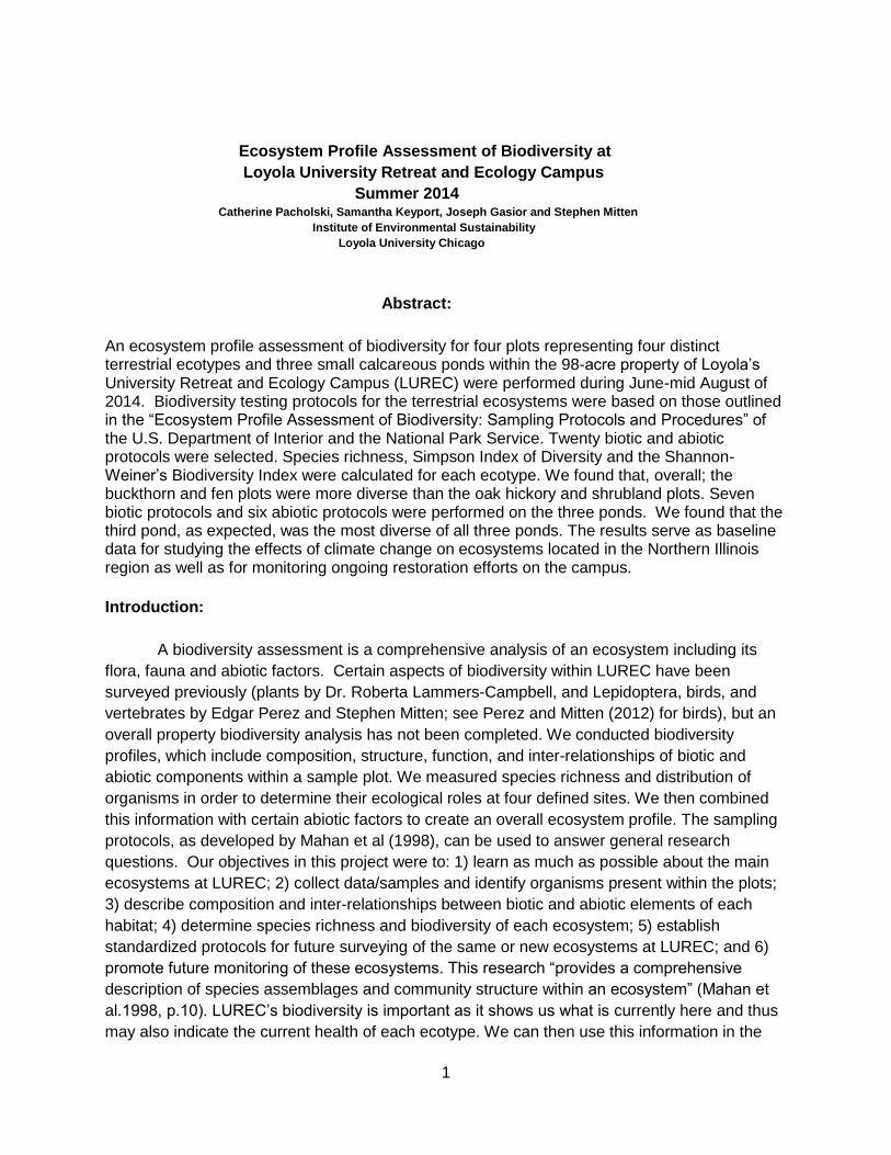
We surveyed four of the main habitat types found at LUREC: oak hickory woodland, shrubland,

degraded calcareous fen wetland, and buckthorn-honeysuckle thicket. The 20 x 20 m plots

were randomly chosen within the general ecosystem type areas and we used GPS to map the

plots on ArcGIS. Figure A below shows each of our study plots on a general map of the LUREC

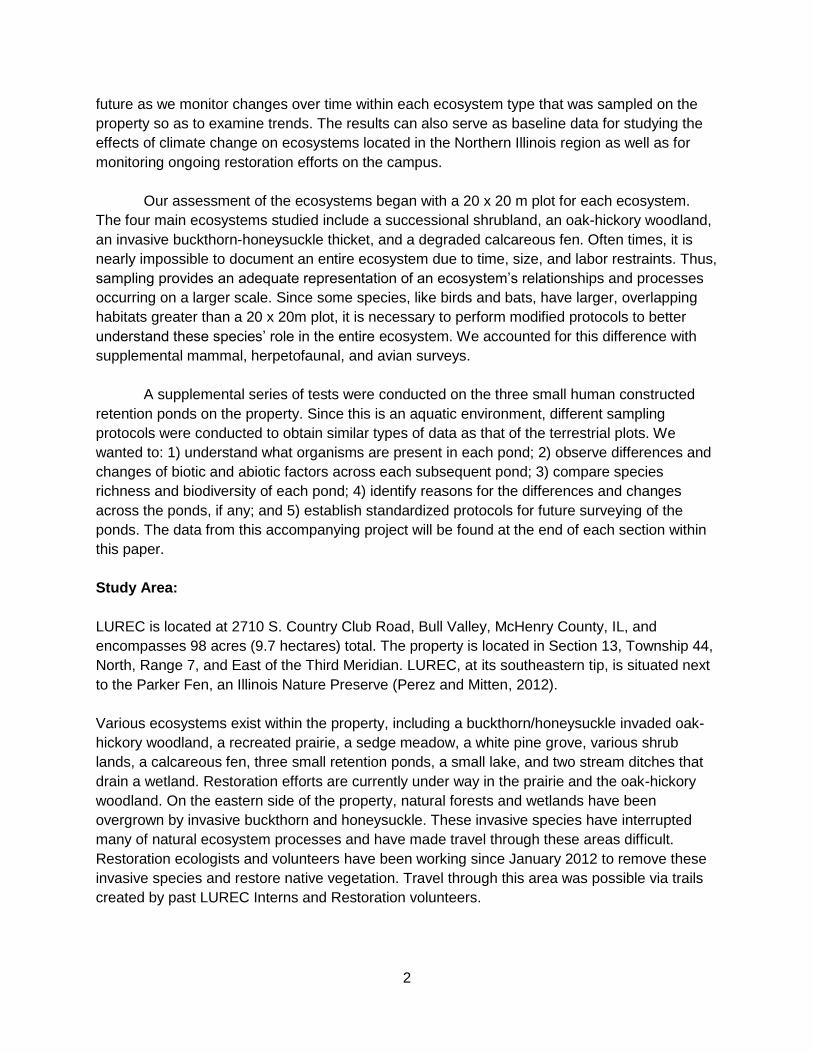
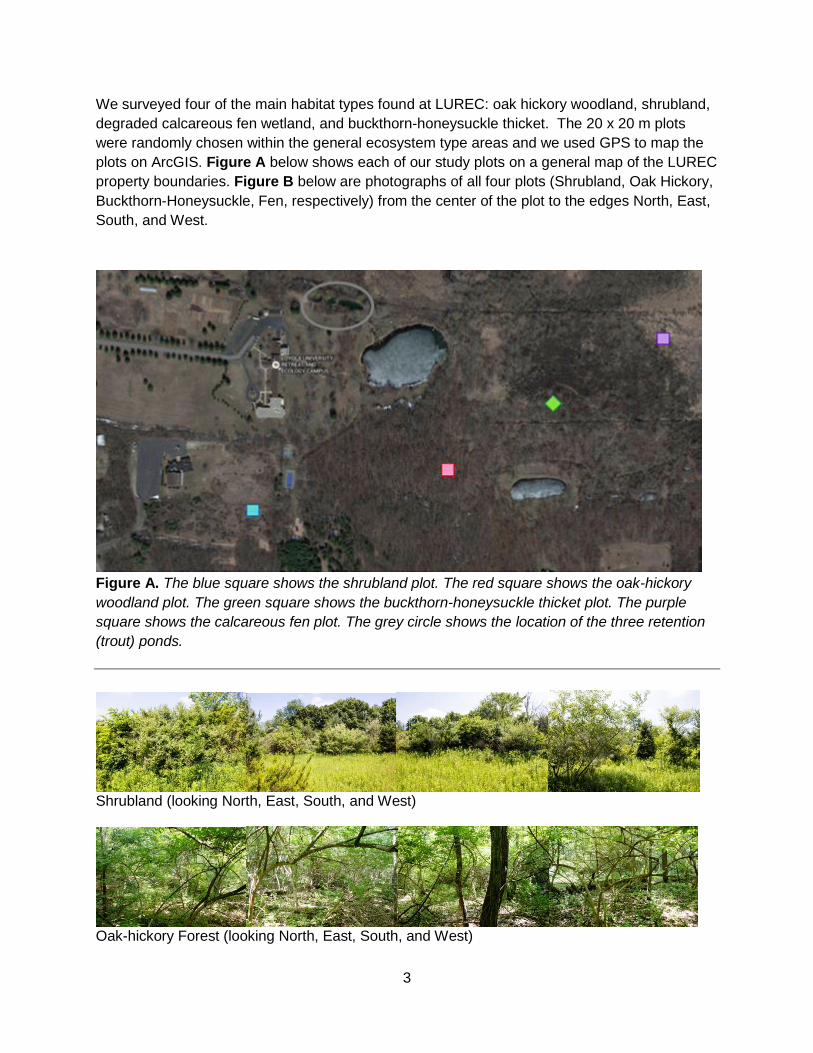
property boundaries. Figure B below are photographs of all four plots (Shrubland, Oak Hickory,

Buckthorn-Honeysuckle, Fen, respectively) from the center of the plot to the edges North, East,

South, and West.

Figure A. The blue square shows the shrubland plot. The red square shows the oak-hickory

woodland plot. The green square shows the buckthorn-honeysuckle thicket plot. The purple

square shows the calcareous fen plot. The grey circle shows the location of the three retention

(trout) ponds.

Shrubland (looking North, East, South, and West)

Oak-hickory Forest (looking North, East, South, and West)

4

Buckthorn-honeysuckle thicket (looking North, East, South, and West)

Degraded fen wetlands (looking North, East, South, and West) Figure B. Photographs of all four plots (Shrubland, Oak Hickory, Buckthorn-Honeysuckle, Fen,

respectively) from the center of the plot to the edges North, East, South, and West.

Methods:

Terrestrial Sampling

Although modified to fit our situation, our sampling methods were based on those laid out in

“Ecosystem Profile Assessment of Biodiversity: Sampling Protocols and Procedures” of the U.S.

Department of Interior and the National Park Service (Mahan et al. 1998).

➢ Terrestrial Biotic

● Herpetofaunal surveys: We overturned all movable objects such as downed logs and

rocks within a 5m radius from the center point of the plot for ten minutes (See Appendix

A). When a herptile was found, the diameter of the object under which it was found was

recorded along with a photograph or notes if the photo was missed. The overturning of

moveable objects was performed once in June and once in July. We also used chance

photography during our research to record any herptiles found, even while performing

other tests or while travelling to other plots.

● Macroinvertebrate surveys: All macroinvertebrates were stored in 95% ethanol unless

otherwise noted. A stereoscope and various online sources and textual dichotomous

keys: Common Spiders of the Chicago Region (Balaban 2012), A Field Guide to the

Insects of America north of Mexico (Borror et al. 1970), How to Know the Immature

Insects (Chu 1949), Kaufman Field Guide to Insects of North America (Eaton et al.

2007), and Photographic Atlas of Entomology and Guide to Insect Identification (Castner

2000) were utilized in order to identify the specimens collected unless otherwise noted

(Mahan et al. 1998).

○ Beating Sheets: Researchers constructed a 1 x 1 m beating sheet using an old

bed sheet and two 1-meter sticks tied in an X pattern to the corners to create a

5

square. Researchers then placed the sheet near vegetation at five random points

within the plot (see Appendix A). We beat the plants 10 times with another

meter stick to agitate invertebrates occupying the vegetation. Any invertebrates

that fell onto the sheet were collected in jars of ethanol, identified, and counted.

This sampling was conducted during shelter seeking time for invertebrates, which

is in the early afternoon or early evening. We collected beating sheet samples

twice, once in June and once in July.

○ Sweeping: The purpose of this test is to collect flying invertebrates. The top of

understory vegetation was swept at a rate of 30 seconds per point for 5 randomly

selected points within each plot (see Appendix A). Invertebrates were collected

using a sweep net (30.4 cm diameter) that was passed side to side in a figure-8

motion. The captured specimens were then placed into jars filled with 70%

ethanol and subsequently identified and counted. We collected sweep net

samples twice; once in June and once in July.

○ Trunk Tree Traps: Trunk tree traps were constructed for the purpose of capturing

tree-dwelling insects. These traps were constructed from a 2L soda bottle, an

Erlenmeyer flask, circular clamps, nails, and a copious amount of duct tape. The

2L bottle was cut so that invertebrates crawling on tree bark could fall into the

Erlenmeyer flask which had had 95% ethanol as a preservative. The top of the

2L bottle was nailed into the the trunk roughly 2 meters from the ground on a

randomly selected tree (see Appendix A). Trunk tree traps were in place for 1

week and refilled with ethanol if necessary over that period. When the sampling

period was over, traps were removed and invertebrates collected, identified, and

counted. There were two sampling periods for this protocol, once in June and

once in July.

○ Light Traps: This test was designed to attract nocturnal invertebrates. Light traps

were made from a 1.5 x 2m fitted bed sheet attached to two large wooden

stakes. The LED light from a Samsung Galaxy s4 cell phone and two

incandescent flashlights illuminated the sheet after 10:00pm, for a period of 10

minutes per plot. Invertebrates attracted to the light source and sheet were

photographed and identified after those initial 10 minutes. Light traps were

conducted near the edge of each test plot once in the month of June.

○ Pitfall Traps: To capture insects that are most active on the habitat floor, we

constructed pitfall traps. We collected invertebrates using 18-ounce plastic cups.

The cups were placed within holes that were dug one week before the collection

period began. The holes were dug at five randomly selected holes within and

along the edges of the plots (see Appendix A). The drinking cups had two small

drainage holes on the side of the cups to prevent flooding from rain events. The

cups were filled approximately 3 ounces with a sea salt-water solution. Pitfalls

were open for a 5 day period, inserted on Monday, checked and collected on

Wednesday and collected and removed on Friday. Specimens were immediately

transferred into 95% ethanol upon return to the laboratory. Pitfall traps were

conducted once in June. Since the majority of the fen was inundated with water,

6

we decided not to conduct pitfall traps at this location since the test would be

ineffective.

● Mammal Trail Cams: Trail cameras (Browning Trail Cam, Model BTC-5 and Plotwatcher

Pro) were placed between 0.5 m and 1 m on a tree above the ground in the 4 plots for

approximately one week each. The camera was placed on a random tree facing inside

the plot. After one week, the data was removed from the camera and analyzed. These

trail cams were placed only once in each plot during the two month testing period.

● Avian Surveys

○ Bird Counts: Point counts were conducted for 7 minute periods at the center of

each plot beginning at 6:00am (see Appendix A). Researchers used Bushnell’s

8 x 42 binoculars. There were two people counting birds and one person who

recorded species type and number. All birds seen or heard within the plot during

the seven minute time period were counted. Birds seen or heard while traveling

to the center of plot along with those that flew over were recorded in a separate

category called “incidentals”. A one minute equilibrium time was observed before

each point count began. These counts were performed at each plot once in June

and once in July.

○ Owl Points: Specific owl sounds were played from the center of three out of four

plots after one minute of silence in the beginning or when switching species (see

Appendix A). Playback was for 15 seconds, with a 45 second pause, 4 times.

Researchers maintained silent and still during this period. Playback was done for

each previously seen species in the area, which includes Eastern Screech Owl

and Great Horned Owl. This test was performed once in early June.

● Flora Surveys

○ Herbaceous Plants: Herbaceous plants were defined as grasses, sedges,

rushes, ferns, and forbs. Cover of herbaceous plants was estimated to the

nearest 5% within a 5 x 5 m plot around the center of the 20 x 20 m plot (see

Appendix A). Herbaceous plants were identified with online sources and textual

resources, primarily Flora of North America: North of Mexico (2007). This test

was conducted once in July.

○ Shrubs: Shrubs were defined as woody plants 0.5-1.4 m in height and less than

2.5 cm in diameter. Cover of shrubs was counted individually within a 10 x 10 m

plot in the center of the 20 x 20 m plot (see Appendix A). Shrubs were identified

with online sources and textual resources, primarily A Field Guide to Trees and

Shrubs: Northeastern and north-central United States and southeastern and

south-central Canada (Petrides 1986). This test was conducted once in July.

○ Saplings: Saplings were defined as woody plants greater than 1.5 m in height

and less than 11.4 cm in diameter. Saplings were counted individually within a 10

x 10 m plot in the center of the 20 x 20m plot, noting any browse or insect

damage (see Appendix A). Saplings were identified in the field or with online

sources and/or textual resources, primarily A Field Guide to Trees and Shrubs:

Northeastern and north-central United States and southeastern and south-central

7

Canada (Petrides 1986), in the lab with photographs. This test was conducted

once in July.

○ Overstory Trees: Overstory trees were defined as woody plants greater than 1.5

m in height and greater than 11.4 cm in diameter. Trees were counted within the

entire 20 x 20 m plot (see Appendix A). Overstory tree identification was done

using textual keys within the field, primarily A Field Guide to Trees and Shrubs:

Northeastern and north-central United States and southeastern and south-central

Canada (Petrides 1986), or using photographs and keys in the lab. This test was

performed once in July.

○ Bryophytes: Bryophyte and lichen samples were collected from a 1 x 0.5m

random point within the 20 x 20 m plot (see Appendix A). Substrate searched

included live wood, dead wood, and rocks. The numbers of different species

were recorded, as was exact species, if possible. Substrate type was also

recorded. Samples were collected in jars and brought back to lab for analysis

using textual and online resources: Bryophytes: Illinois Bryhophytes (2006). This

test was conducted once in June.

➢ Terrestrial Abiotic

● Canopy Cover: Canopy cover was estimated by percentage from the four corners and at

the center of the 20 x 20 m plot by estimating how much of our field of view when looking

upward was covered by foliage and performed by the same viewer for each of the four

plots. Percentages were estimated to the closest 10%. Each test was completed on days

of full sun, once in June and once in July.

● Leaf Litter Samples: Leaf litter samples were collected by hand in approximately 0.25 x

0.25 m section at five random points within each ecosystem (see Appendix A). These

samples were taken at the same location as soil cores. Samples were placed in plastic

bags which were sealed and stored in a freezer at 5 degree Celsius for seven days.

After this period, the samples were thawed and the weight was recorded. The samples

were then dried using a scientific drying oven. The dry weight was recorded. This test

was performed twice, once in June and once in July.

● Distance to Edge: A rangefinder (Bushnell Yardage Pro Sport 450) was used to

calculate distance to edge (meaning the distance to the nearest edge created by a

change in general habitat type (e.g., forest stand edge, stream, road)). One person took

readings facing each cardinal direction from the midpoint of the center of the plot. The

rangefinder was pointed at a habitat that was different than the ecosystem being studied.

This value was recorded in yards as distance to edge. This test was conducted once per

plot.

● Soil Chemistry: Soil cores were taken at the same place as leaf litter samples, which

were five random points within each plot (see Appendix A). These cores were sampled

using 12-inch soil corer. The middle six inches of each core of the five samples were

collected in one plastic bag for each plot. The bags were brought back to the lab and

frozen until analysis was performed. When this happened, bags were thawed and tested

for pH, potassium (lb/acre), phosphorus (lb/acre), and nitrogen (lb/acre) using a soil

macronutrient testing kit (LaMotte, Code 5928). Soil texture and type were also analyzed

8

and recorded (USDA Soil Texturing Field Flow Chart). A hand soil pH tester was also

used to supplement our data (Kelway Soil Tester). Soil cores were sampled twice per

plot, once in June and once in July.

● Water Chemistry: Water chemistry was measured only in the fen using a YSI

Environmental tool (Model 556). This instrument gives data for temperature (degrees

Celsius), electrolytic conductivity, or ion content (ms/cm^c), electrical resistance (Ω*cm),

total dissolved solids (TDS, g/L), salinity (sal), dissolved oxygen (D.O., mg/L), pH, and

reduction potential (ORP). The fen water quality was taken three times in one sampling

and the results were averaged to give a single value. The test was performed twice in

the fen, once in June and once in July when water was present.

● Elevation: We used a GPS (Garmin GPSmap 62s) to get an elevation calculation. Four

samples were taken and averaged to get a final value. This test was performed once per

plot.

Aquatic Sampling

All protocols were based on those performed by Loyola University Chicago’s Biology

Department’s “Biotic and Abiotic Profile of Dufield Pond, Woodstock IL” (2013), as well as the

“Ecosystem Profile Assessment of Biodiversity: Sampling Protocols and Procedures” of the U.S.

Department of Interior and the National Park Service (Mahan et al. 1998).

➢ Aquatic Biotic

● Macroinvertebrates: Macroinvertebrates were collected using a 12 x 6 in. fine mesh net

with a 6 ft. long handle in order to collect specimens. One sample was taken from the

limnetic zone and another from the benthic zone at three random locations of each pond,

for a total of six samples per pond. All six samples were collected in a single jar for each

pond. These samples were taken back to lab for analysis using a stereoscope and

various textual and online identification resources: Guide to Aquatic Invertebrates of the

Upper Midwest (Bouchard et al. 2004), An Introduction to the Aquatic Insects of North

America (Merritt, 2008), Key to Common Macroinvertabrates (2014). We recorded

number of specimens to the taxonomic order to which they belong. This protocol was

performed once in late July.

○ Dragonflies and damselflies were observed over the ponds and identified in the

lab with the use of online sources and textual keys.

● Microinvertebrates:

○ Phytoplankton were collected using a plankton net trap. The trap was thrown

once into the center of a pond and dragged into shore by the researcher. This

was conducted one time for each pond. The contents of the net were then

emptied into a jar for analysis. Only one sample was collected at a time to ensure

that organisms were living when observed under the compound microscope.

From the bottom of each jar, 10 drops were taken and one drop was placed on

each slide. We observed each slide for five minutes and recorded all

phytoplankton species seen within that time frame (filamentous, non-filamentous,

or diatom). Online and textual sources were used to identify each type of

phytoplankton: Guide to Identification of Fresh Water Microorganisms (Walker et

al. 2000).

9

○ Zooplankton were collected using jars from each cardinal direction in the benthic

zone one meter from the edge of the pond. Only one sample was taken at a time

to ensure that all organisms were living when analyzed. Jars were brought into

the lab for analysis under a compound microscope. From the bottom of each jar,

10 drops were taken and one drop was placed on each slide. We observed each

slide for five minutes and recorded all zooplankton species seen within that time

frame (protozoa [ciliates, heliozoans, flagellates, and amoebas], rotifers,

roundworms, flatworms, cladocerans, copepods, ostracods, water mites,

oligochaetes, gastrotricha, tardigrades, and insect larvae). Online and textual

sources were used to identify each type of zooplankton: Dichotomous Key for

Protozoa (n.d.), A Guide to the Freshwater Calanoid and Cyclopoid Copepod

Crustacea of Ontario (Smith et al. 1978), Guide to Identification of Fresh Water

Microorganisms (Walker et al. 2000), An Illustrated Guide to the Identification of

the Planktonic Crustacea of Lake Michigan (Torke, 1974), , and Protoctista

(a.k.a. Protists) (Duffie et al. 2012).

○ Both tests were performed once at the end of July.

● Vegetation: Submerged underwater vegetation (SUV) in the ponds was identified

recorded. This was conducted once at the beginning of August.

● Herptiles: Species types and number observed of herptiles were recorded for each pond.

This test was performed each time we visited the ponds.

● Avian Species: Avian species were noted each time we visited the ponds.

➢ Aquatic Abiotic

● Turbidity: A secchi disk was used to determine turbidity as close to center of the pond as

possible. The disk was dropped from the surface of pond and slowly lowered via rope

into the water until the black and white pattern was no longer visible to the researcher.

The depth at which this occurred was recorded by measuring the length of the rope.

Thus, turbidity was measured in centimeters. This was conducted once per pond at the

end of July.

● Area/Volume and Depth at Center: Average length, width, and height were measured

using a transect measuring tape, and area and volume were calculated with this data.

The depth at center was calculated using slope method. This was calculated once per

pond.

● Bank Condition/Substrates: Bank condition and substrates were analyzed visually.

Descriptions were recorded once per pond at the end of July.

● Canopy cover: Canopy cover was estimated by percentage from the four cardinal

directions at the edge and at the center of each pond. Percentages were estimated to

the closest 10%. Each test was completed on a day of full sun, once at the end of July.

● Water Chemistry: The YSI tool (Model 556) was also used for pond analysis. We

brought the probe to the center of the pond and dropped it to the bottom. Three samples

were recorded when the values stabilized, and an average was taken. This instrument

gives data for temperature (degrees Celsius), electrolytic conductivity, or ion content

(ms/cm^c), electrical resistance (Ω*cm), total dissolved solids (TDS, g/L), salinity (sal),

dissolved oxygen (D.O., mg/L), pH, and reduction potential (ORP). Each pond’s water

10

quality was taken three times in one sampling and the results were averaged to give a

single value. This test was performed once at each pond at the end of July.

● General Observations: General ecosystem observations of each pond were recorded

whenever we visited to take samples.

Results:

Terrestrial Results

FEN:

Using the Simpson Index of Diversity, we calculated the overall biodiversity (1-D) within the fen

to be 0.9676. Likewise, using Shannon-Weiner’s Biodiversity Index, we calculated overall

biodiversity (H’) at this location to be 4.051. Species richness for this plot habitat was calculated

to be 90 overall (see Appendix B).

We found 4 different species of herptiles, including Western Chorus Frog (Pseudacris triseriata),

Plains Leopard Frog (Lithobates blairi), American Toad (Anaxyrus americanus), and Eastern

Milk Snake (Lampropeltis triangulum triangulum).

No images of vertebrates were captured on the trail camera at the fen.

For avian biodiversity, we recorded 19 different species of birds during the two month testing

period. Overall, the most abundant bird species observed in this location was the Red-winged

Blackbird (Agelaius phoeniceus). For a list of all the birds found here, please see Appendix B.

While owl point counts were performed, no species were observed because it was outside of

the breeding season.

Macroinvertebrates were collected using four tests in the fen. These tests collected flying

insects (sweeping), insects dwelling in trees and in forbs (trunk tree traps and beating sheets),

and nocturnal flying insects (light traps). We found a total of 53 different species in this

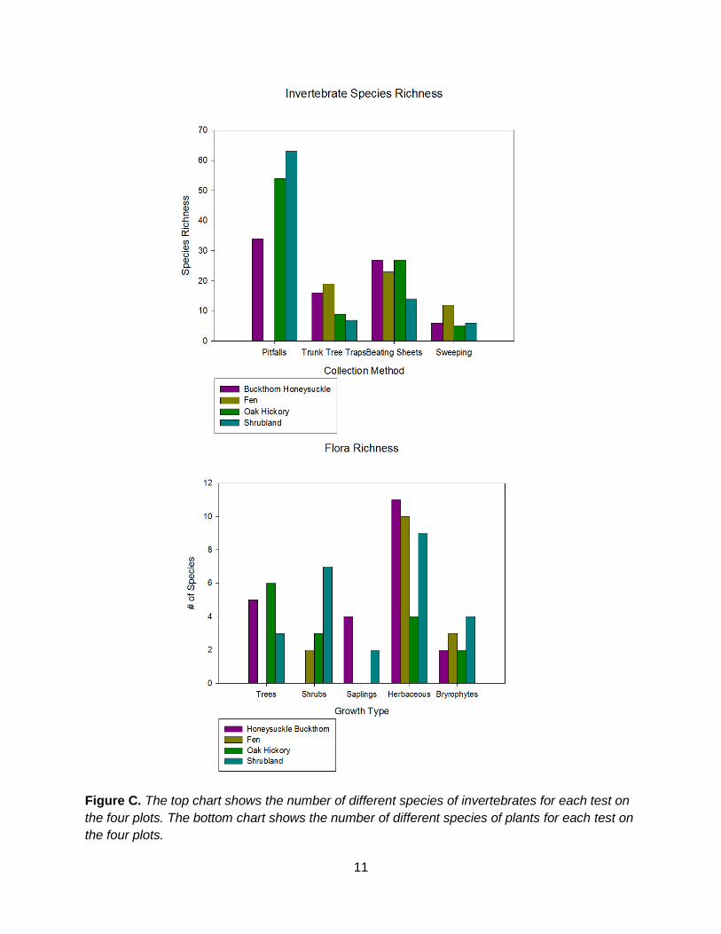
ecosystem. The effectiveness of these tests varied, but Figure C below shows number of

species found relating to each test for all four transects. The graph shows that the sweeping

collected 12 species of insects, beating sheets with 23 species, and trunk tree traps with 19

species. Unfortunately, the light trap data was not collected because the camera lens could not

magnify the macroinvertebrates adequately at night. A list of all macroinvertebrate species

observed in the fen can be found in Appendix B. Please note: due to the wet conditions of the

fen, invertebrate pitfall trap samplings were unable to be performed.

11

Figure C. The top chart shows the number of different species of invertebrates for each test on

the four plots. The bottom chart shows the number of different species of plants for each test on

the four plots.

12

Flora surveys provided a representation of the fen plant diversity. Flora types were separated

into five categories: herbaceous plants, shrubs, saplings, overstory trees, and bryophytes. A

total of 15 different species of flora were observed in the fen. Figure C above displays species

richness of each type of flora found in the fen and the other three transects. The graph shows

that there were 10 herbaceous plant species, 2 shrub species, 0 sapling species, 0 overstory

tree species, and 3 bryophyte species. A list of all flora noted in the fen can be found in

Appendix B.

.

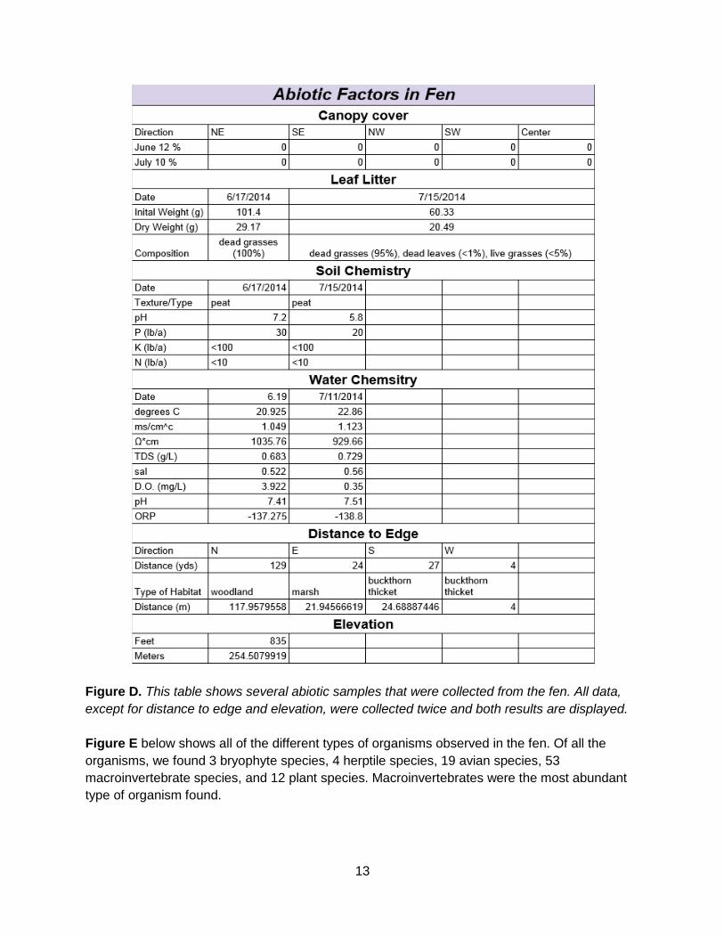
Figure D below shows the abiotic factors that influence the fen ecosystem. We collected

information for canopy cover, leaf litter, soil chemistry, distance to edge, and elevation. We were

able also to conduct water chemistry analyses at this site because of the standing water.

Throughout this entire plot, there was 0% canopy cover in all directions during both testing

dates in June and July. Slightly more leaf litter was collected during June than in July, consisting

of 29.17 grams of dead grasses compared to 20.49 grams of dead grasses, leaves, and live

grasses in July. In relation to soil chemistry, the most prominent data collected was pH, which

fluctuated from 7.2 to become slightly more acidic in July at 5.8 respectively. Potassium,

Nitrogen and Phosphorous loads were all low in this location. In relation to water chemistry,

dissolved oxygen content had the most significant data change between June and July, ranging

from 3.922 (mg/L) to 0.35 (mg/L). In observance of distance to edge, various habitats were

observed from the center of the plot. Roughly 118 meters to the north, oak woodland is the

closest bordering habitat. To the east, marsh habitat lies at a distance of 22 meters. A buckthorn

thicket is observed roughly 25 meters south of the test plot and 4 meters west of the test plot.

The elevation of this test plot is about 254.5 meters.

13

Figure D. This table shows several abiotic samples that were collected from the fen. All data,

except for distance to edge and elevation, were collected twice and both results are displayed.

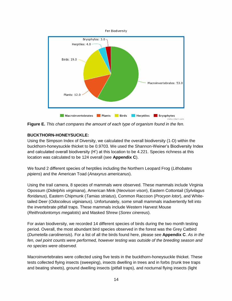
Figure E below shows all of the different types of organisms observed in the fen. Of all the

organisms, we found 3 bryophyte species, 4 herptile species, 19 avian species, 53

macroinvertebrate species, and 12 plant species. Macroinvertebrates were the most abundant

type of organism found.

14

Figure E. This chart compares the amount of each type of organism found in the fen.

BUCKTHORN-HONEYSUCKLE:

Using the Simpson Index of Diversity, we calculated the overall biodiversity (1-D) within the

buckthorn-honeysuckle thicket to be 0.9703. We used the Shannon-Weiner’s Biodiversity Index

and calculated overall biodiversity (H’) at this location to be 4.221. Species richness at this

location was calculated to be 124 overall (see Appendix C).

We found 2 different species of herptiles including the Northern Leopard Frog (Lithobates

pipiens) and the American Toad (Anaxyrus americanus).

Using the trail camera, 8 species of mammals were observed. These mammals include Virginia

Opossum (Didelphis virginiana), American Mink (Neovison vison), Eastern Cottontail (Sylvilagus

floridanus), Eastern Chipmunk (Tamias striatus), Common Raccoon (Procyon lotor), and White-

tailed Deer (Odocoileus viginianus). Unfortunately, some small mammals inadvertently fell into

the invertebrate pitfall traps. These mammals include Western Harvest Mouse

(Reithrodontomys megalotis) and Masked Shrew (Sorex cinereus).

For avian biodiversity, we recorded 14 different species of birds during the two month testing

period. Overall, the most abundant bird species observed in the forest was the Grey Catbird

(Dumetella carolinensis). For a list of all the birds found here, please see Appendix C. As in the

fen, owl point counts were performed, however testing was outside of the breeding season and

no species were observed.

Macroinvertebrates were collected using five tests in the buckthorn-honeysuckle thicket. These

tests collected flying insects (sweeping), insects dwelling in trees and in forbs (trunk tree traps

and beating sheets), ground dwelling insects (pitfall traps), and nocturnal flying insects (light

15

traps). We found a total of 73 different species of macroinvertebrates in this ecosystem. The

effectiveness of these tests varied, but Figure C above shows number of species found relating

to each test compared to all three plots. The graph shows that the sweeping collected 6

species, beating sheets with 27 species, the pitfall traps with 34 species, and trunk tree traps

with 16 species. Unfortunately, the light trap data was not collected because the camera lens

could not magnify the macroinvertebrates adequately at night. A list of all invertebrate species

observed in this plot can be found in Appendix C.

Flora surveys provided a representation of the buckthorn-honeysuckle thicket plant diversity.

Flora types were separated into five categories: herbaceous plants, shrubs, saplings, overstory

trees, and bryophytes. A total of 20 species of flora were noted in the buckthorn-honeysuckle

thicket. Figure C above displays species richness of each type of flora found where these

invasive plants have seemed to take over. The graph shows that there were 11 herbaceous

plant species, 0 shrub species, 4 sapling species, 5 overstory tree species, and 2 bryophyte

species. A list of all flora noted at this location can be found in Appendix C.

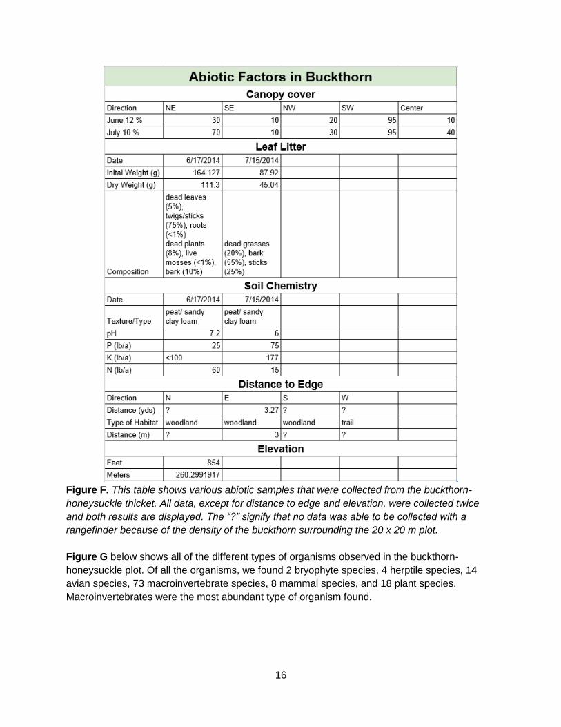
Figure F below shows the abiotic factors that influence the buckthorn-honeysuckle thicket’s

ecosystem. We collected information for canopy cover, leaf litter, soil chemistry, distance to

edge, and elevation. Throughout this entire plot, canopy cover was most prominent in the

southwest location of the plot, at 95%. Canopy cover also increased the most between the June

and July testing dates in the northeast direction, fluctuating from 30% to 70%. Leaf litter

collection was much more prominent during June than in July, consisting of 111.3 grams of

dead leaves, plants, twigs, roots, bark and live mosses compared to 45.04 grams of dead

grasses, barks, and sticks in July. In relation to soil chemistry, the most prominent data

collected was phosphorous and nitrogen. Phosphorous load fluctuated from 25 lb/acre to 75

lb/acre between June and July. Nitrogen load decreased between June and July, going from 60

lb/acre to 15 lb/acre. Potassium load also increased from less than 100 lb/acre in June to 177

lb/acre in July. In observance of distance to edge, a similar habitat of woodland was observed in

all cardinal directions, save for the trail that was observable to the west of the testing plot. The

distance of each of these habitats from the center of the plot was difficult to measure due to the

density of the thicket itself. The elevation of this test plot is about 260 meters.

16

Figure F. This table shows various abiotic samples that were collected from the buckthorn-

honeysuckle thicket. All data, except for distance to edge and elevation, were collected twice

and both results are displayed. The “?” signify that no data was able to be collected with a

rangefinder because of the density of the buckthorn surrounding the 20 x 20 m plot.

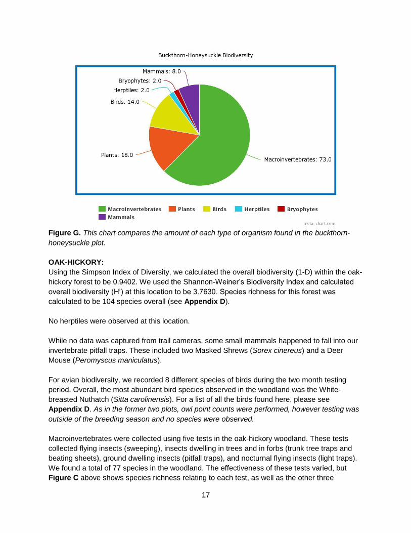
Figure G below shows all of the different types of organisms observed in the buckthorn-

honeysuckle plot. Of all the organisms, we found 2 bryophyte species, 4 herptile species, 14

avian species, 73 macroinvertebrate species, 8 mammal species, and 18 plant species.

Macroinvertebrates were the most abundant type of organism found.

17

Figure G. This chart compares the amount of each type of organism found in the buckthorn-

honeysuckle plot.

OAK-HICKORY:

Using the Simpson Index of Diversity, we calculated the overall biodiversity (1-D) within the oak-

hickory forest to be 0.9402. We used the Shannon-Weiner’s Biodiversity Index and calculated

overall biodiversity (H’) at this location to be 3.7630. Species richness for this forest was

calculated to be 104 species overall (see Appendix D).

No herptiles were observed at this location.

While no data was captured from trail cameras, some small mammals happened to fall into our

invertebrate pitfall traps. These included two Masked Shrews (Sorex cinereus) and a Deer

Mouse (Peromyscus maniculatus).

For avian biodiversity, we recorded 8 different species of birds during the two month testing

period. Overall, the most abundant bird species observed in the woodland was the White-

breasted Nuthatch (Sitta carolinensis). For a list of all the birds found here, please see

Appendix D. As in the former two plots, owl point counts were performed, however testing was

outside of the breeding season and no species were observed.

Macroinvertebrates were collected using five tests in the oak-hickory woodland. These tests

collected flying insects (sweeping), insects dwelling in trees and in forbs (trunk tree traps and

beating sheets), ground dwelling insects (pitfall traps), and nocturnal flying insects (light traps).

We found a total of 77 species in the woodland. The effectiveness of these tests varied, but

Figure C above shows species richness relating to each test, as well as the other three

18

ecosystems. The graph shows that the sweeping collected 5 species, beating sheets with 27

species, the pitfall traps with 54 species, and trunk tree traps with 9 species. Unfortunately, the

light trap data was not collected because the camera lens could not magnify the

macroinvertebrates adequately at night. A list of all invertebrate species observed in this plot

can be found in Appendix D.

Flora surveys provided a representation of the oak-hickory woodland plant diversity. Flora types

were separated into five categories: herbaceous plants, shrubs, saplings, overstory trees, and

bryophytes. A total of 15 different species of flora were found in the oak-hickory woodland.

Figure C above displays species richness of each type of flora found. The graph shows that

there were 4 herbaceous plant species, 3 shrub species, 0 sapling species, 6 overstory tree

species, and 2 bryophyte species. A list of all flora noted at this location can be found in

Appendix D.

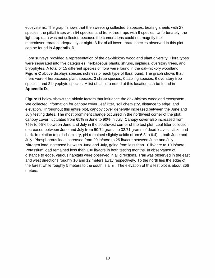
Figure H below shows the abiotic factors that influence the oak-hickory woodland ecosystem.

We collected information for canopy cover, leaf litter, soil chemistry, distance to edge, and

elevation. Throughout this entire plot, canopy cover generally increased between the June and

July testing dates. The most prominent change occurred in the northwest corner of the plot;

canopy cover fluctuated from 65% in June to 90% in July. Canopy cover also increased from

75% to 95% between June and July in the southwest corner of the test plot. Leaf litter collection

decreased between June and July from 50.74 grams to 32.71 grams of dead leaves, sticks and

bark. In relation to soil chemistry, pH remained slightly acidic (from 6.8 to 6.4) in both June and

July. Phosphorous load increased from 20 lb/acre to 25 lb/acre between June and July.

Nitrogen load increased between June and July, going from less than 10 lb/acre to 10 lb/acre.

Potassium load remained less than 100 lb/acre in both testing months. In observance of

distance to edge, various habitats were observed in all directions. Trail was observed in the east

and west directions roughly 10 and 12 meters away respectively. To the north lies the edge of

the forest while roughly 5 meters to the south is a hill. The elevation of this test plot is about 266

meters.

19

Figure H. This table shows several abiotic samples that were cumulated from the oak-hickory

forest. All data, except for distance to edge and elevation, were collected twice and the results

from both dates are displayed. The “?” signify that no data was able to be collected with a

rangefinder because of the density and vastness of the woodland.

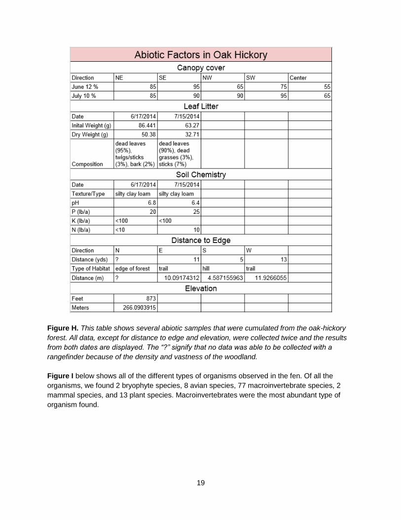
Figure I below shows all of the different types of organisms observed in the fen. Of all the

organisms, we found 2 bryophyte species, 8 avian species, 77 macroinvertebrate species, 2

mammal species, and 13 plant species. Macroinvertebrates were the most abundant type of

organism found.

20

Figure I. This chart compares the amount of each type of organism found in the oak-hickory

woodland.

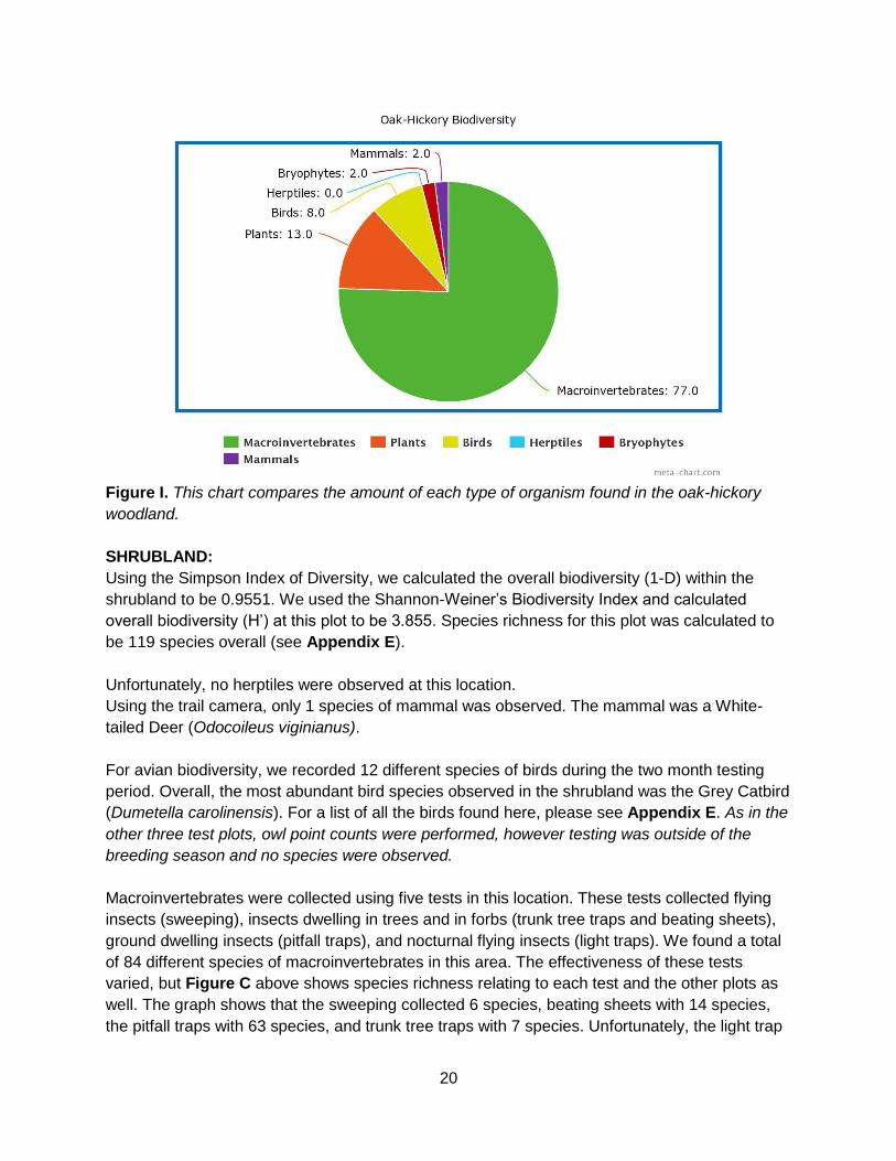
SHRUBLAND:

Using the Simpson Index of Diversity, we calculated the overall biodiversity (1-D) within the

shrubland to be 0.9551. We used the Shannon-Weiner’s Biodiversity Index and calculated

overall biodiversity (H’) at this plot to be 3.855. Species richness for this plot was calculated to

be 119 species overall (see Appendix E).

Unfortunately, no herptiles were observed at this location.

Using the trail camera, only 1 species of mammal was observed. The mammal was a White-

tailed Deer (Odocoileus viginianus).

For avian biodiversity, we recorded 12 different species of birds during the two month testing

period. Overall, the most abundant bird species observed in the shrubland was the Grey Catbird

(Dumetella carolinensis). For a list of all the birds found here, please see Appendix E. As in the

other three test plots, owl point counts were performed, however testing was outside of the

breeding season and no species were observed.

Macroinvertebrates were collected using five tests in this location. These tests collected flying

insects (sweeping), insects dwelling in trees and in forbs (trunk tree traps and beating sheets),

ground dwelling insects (pitfall traps), and nocturnal flying insects (light traps). We found a total

of 84 different species of macroinvertebrates in this area. The effectiveness of these tests

varied, but Figure C above shows species richness relating to each test and the other plots as

well. The graph shows that the sweeping collected 6 species, beating sheets with 14 species,

the pitfall traps with 63 species, and trunk tree traps with 7 species. Unfortunately, the light trap

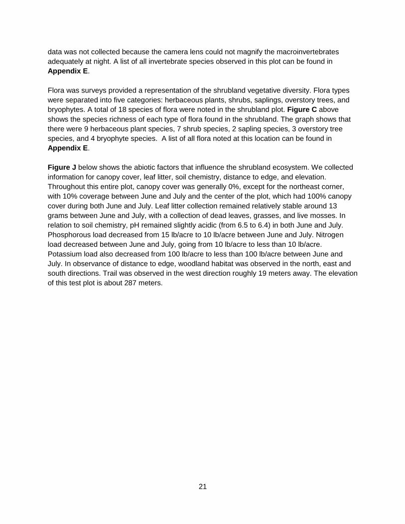
21

data was not collected because the camera lens could not magnify the macroinvertebrates

adequately at night. A list of all invertebrate species observed in this plot can be found in

Appendix E.

Flora was surveys provided a representation of the shrubland vegetative diversity. Flora types

were separated into five categories: herbaceous plants, shrubs, saplings, overstory trees, and

bryophytes. A total of 18 species of flora were noted in the shrubland plot. Figure C above

shows the species richness of each type of flora found in the shrubland. The graph shows that

there were 9 herbaceous plant species, 7 shrub species, 2 sapling species, 3 overstory tree

species, and 4 bryophyte species. A list of all flora noted at this location can be found in

Appendix E.

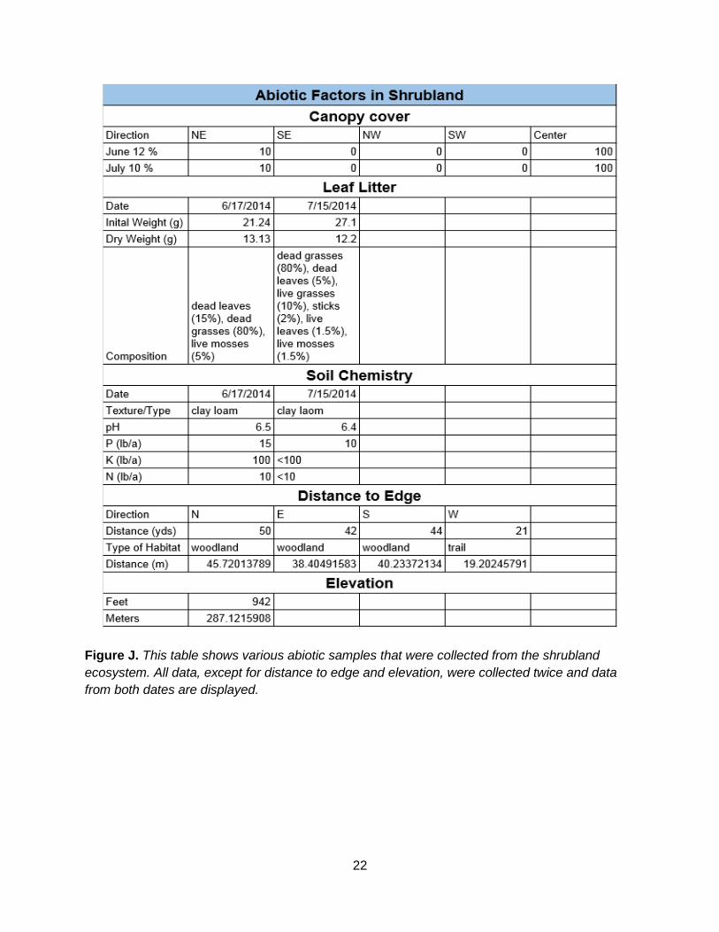
Figure J below shows the abiotic factors that influence the shrubland ecosystem. We collected

information for canopy cover, leaf litter, soil chemistry, distance to edge, and elevation.

Throughout this entire plot, canopy cover was generally 0%, except for the northeast corner,

with 10% coverage between June and July and the center of the plot, which had 100% canopy

cover during both June and July. Leaf litter collection remained relatively stable around 13

grams between June and July, with a collection of dead leaves, grasses, and live mosses. In

relation to soil chemistry, pH remained slightly acidic (from 6.5 to 6.4) in both June and July.

Phosphorous load decreased from 15 lb/acre to 10 lb/acre between June and July. Nitrogen

load decreased between June and July, going from 10 lb/acre to less than 10 lb/acre.

Potassium load also decreased from 100 lb/acre to less than 100 lb/acre between June and

July. In observance of distance to edge, woodland habitat was observed in the north, east and

south directions. Trail was observed in the west direction roughly 19 meters away. The elevation

of this test plot is about 287 meters.

22

Figure J. This table shows various abiotic samples that were collected from the shrubland

ecosystem. All data, except for distance to edge and elevation, were collected twice and data

from both dates are displayed.

23

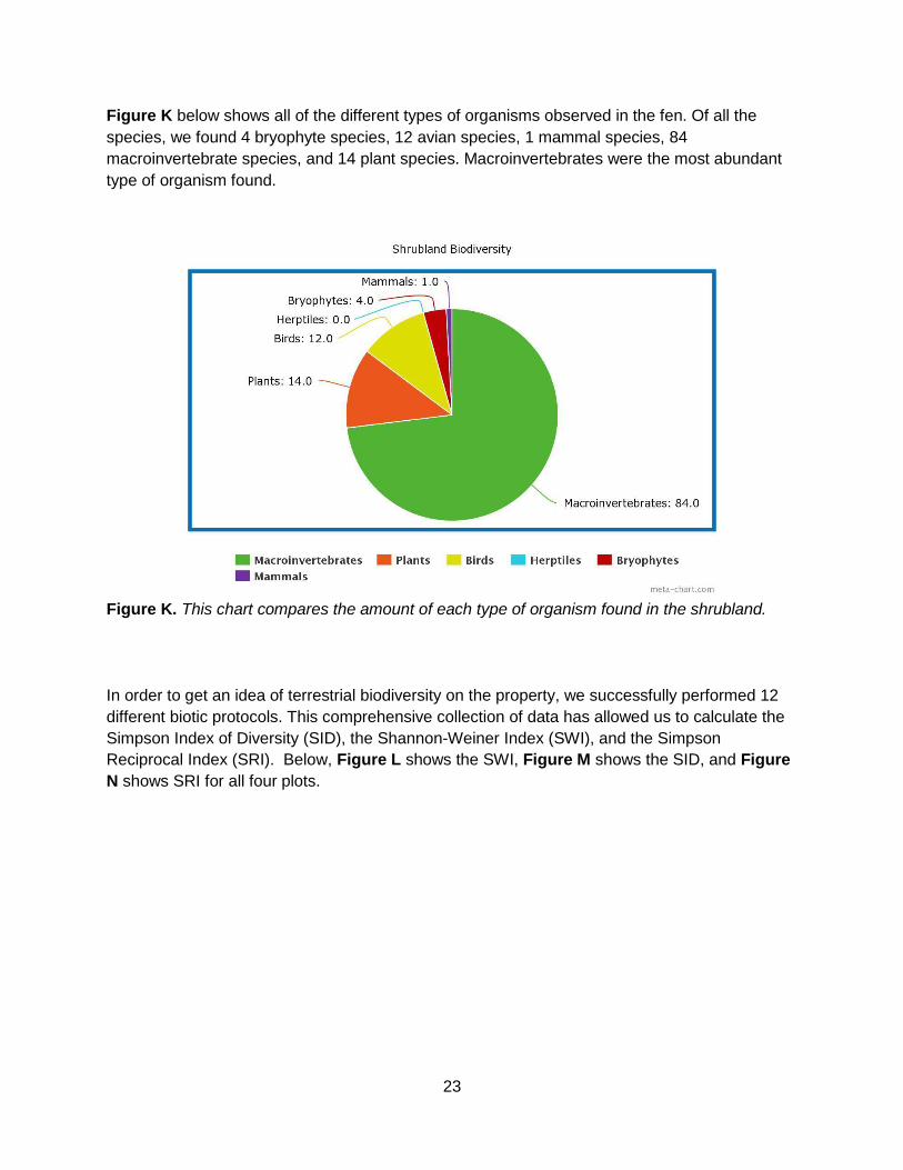
Figure K below shows all of the different types of organisms observed in the fen. Of all the

species, we found 4 bryophyte species, 12 avian species, 1 mammal species, 84

macroinvertebrate species, and 14 plant species. Macroinvertebrates were the most abundant

type of organism found.

Figure K. This chart compares the amount of each type of organism found in the shrubland.

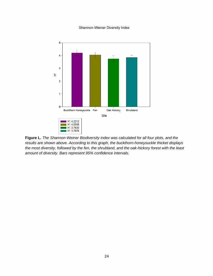
In order to get an idea of terrestrial biodiversity on the property, we successfully performed 12

different biotic protocols. This comprehensive collection of data has allowed us to calculate the

Simpson Index of Diversity (SID), the Shannon-Weiner Index (SWI), and the Simpson

Reciprocal Index (SRI). Below, Figure L shows the SWI, Figure M shows the SID, and Figure

N shows SRI for all four plots.

24

Figure L. The Shannon-Weiner Biodiversity index was calculated for all four plots, and the

results are shown above. According to this graph, the buckthorn-honeysuckle thicket displays

the most diversity, followed by the fen, the shrubland, and the oak-hickory forest with the least

amount of diversity. Bars represent 95% confidence intervals.

25

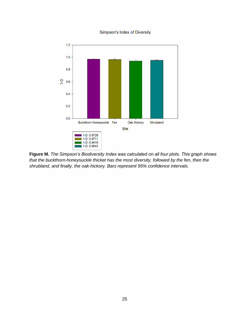
Figure M. The Simpson’s Biodiversity Index was calculated on all four plots. This graph shows

that the buckthorn-honeysuckle thicket has the most diversity, followed by the fen, then the

shrubland, and finally, the oak-hickory. Bars represent 95% confidence intervals.

26

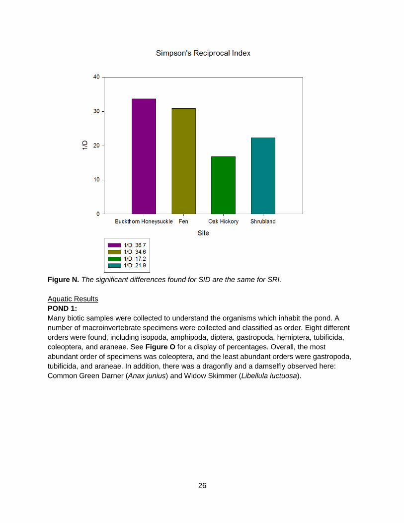
Figure N. The significant differences found for SID are the same for SRI.

Aquatic Results

POND 1:

Many biotic samples were collected to understand the organisms which inhabit the pond. A

number of macroinvertebrate specimens were collected and classified as order. Eight different

orders were found, including isopoda, amphipoda, diptera, gastropoda, hemiptera, tubificida,

coleoptera, and araneae. See Figure O for a display of percentages. Overall, the most

abundant order of specimens was coleoptera, and the least abundant orders were gastropoda,

tubificida, and araneae. In addition, there was a dragonfly and a damselfly observed here:

Common Green Darner (Anax junius) and Widow Skimmer (Libellula luctuosa).

27

Figure O. This chart represents a comparison of amount of different orders of

macroinvertebrates found in the first pond.

Zooplankton were collected and recorded by order. We classified phytoplankton as either

filamentous, non-filamentous, or diatoms. All three were found to be present in Pond 1. The

most abundant of these were non-filamentous plankton. Also in the pond, 14 different types of

zooplankton were observed. These include heliozoans, ciliates, flagellates, amoebas,

copepods, rotifers, roundworms, flatworms, water mites, cladocerans, gastrotrichs, ostracods,

isopods, and mosquito larvae. Figure P shows a chart of microinvertebrate percentages found

in this pond.

Figure P. The two charts above represent both amounts of phytoplankton and amounts of

zooplankton found in Pond 1. The “other” category in the Zooplankton chart includes rotifers,

mosquito larvae, ostracods, flatworms.

28

Five different types of vegetation were found growing in the pond. These include musk grass

(Chara spp.), watercress (Nasturtium officinale), reed canary grass (Phalaris arundinacea),

duckweed (Lemnaceae), and spike rush (Eleocharis spp.).

Two species of frogs were observed at this location: 18 Western Chorus Frogs (Pseudacris

triseriata) and 1 American Bullfrog (Lithobates catesbeianus).

Two species of birds were observed over the pond: American Robin (Turdus migratorius) and

American Goldfinch (Carduelis Tristis).

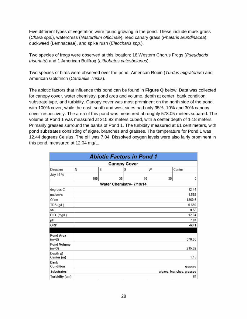
The abiotic factors that influence this pond can be found in Figure Q below. Data was collected

for canopy cover, water chemistry, pond area and volume, depth at center, bank condition,

substrate type, and turbidity. Canopy cover was most prominent on the north side of the pond,

with 100% cover, while the east, south and west sides had only 35%, 10% and 30% canopy

cover respectively. The area of this pond was measured at roughly 578.05 meters squared. The

volume of Pond 1 was measured at 215.82 meters cubed, with a center depth of 1.18 meters.

Primarily grasses surround the banks of Pond 1. The turbidity measured at 61 centimeters, with

pond substrates consisting of algae, branches and grasses. The temperature for Pond 1 was

12.44 degrees Celsius. The pH was 7.04. Dissolved oxygen levels were also fairly prominent in

this pond, measured at 12.04 mg/L.

29

Figure Q. This table shows data collected for various abiotic tests that were performed for Pond

1. The water chemistry data was taken three times and the average value is displayed above.

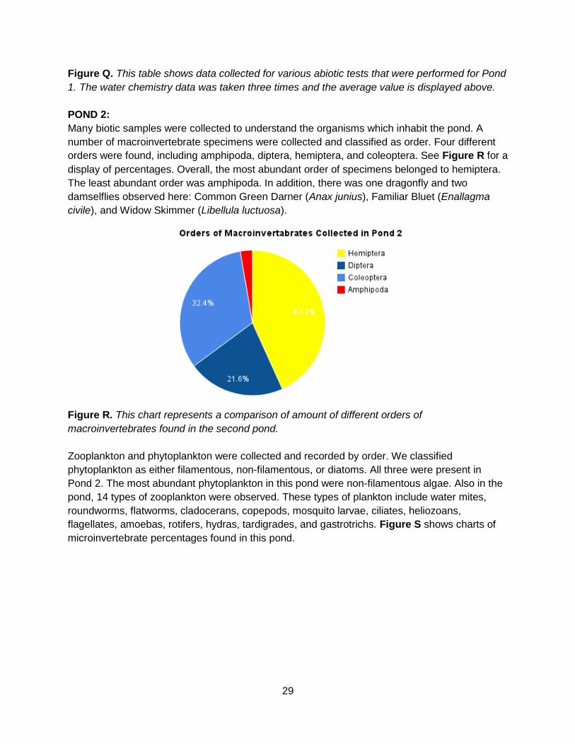
POND 2:

Many biotic samples were collected to understand the organisms which inhabit the pond. A

number of macroinvertebrate specimens were collected and classified as order. Four different

orders were found, including amphipoda, diptera, hemiptera, and coleoptera. See Figure R for a

display of percentages. Overall, the most abundant order of specimens belonged to hemiptera.

The least abundant order was amphipoda. In addition, there was one dragonfly and two

damselflies observed here: Common Green Darner (Anax junius), Familiar Bluet (Enallagma

civile), and Widow Skimmer (Libellula luctuosa).

Figure R. This chart represents a comparison of amount of different orders of

macroinvertebrates found in the second pond.

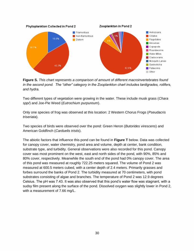
Zooplankton and phytoplankton were collected and recorded by order. We classified

phytoplankton as either filamentous, non-filamentous, or diatoms. All three were present in

Pond 2. The most abundant phytoplankton in this pond were non-filamentous algae. Also in the

pond, 14 types of zooplankton were observed. These types of plankton include water mites,

roundworms, flatworms, cladocerans, copepods, mosquito larvae, ciliates, heliozoans,

flagellates, amoebas, rotifers, hydras, tardigrades, and gastrotrichs. Figure S shows charts of

microinvertebrate percentages found in this pond.

30

Figure S. This chart represents a comparison of amount of different macroinvertebrates found

in the second pond. The “other” category in the Zooplankton chart includes tardigrades, rotifers,

and hydra.

Two different types of vegetation were growing in the water. These include musk grass (Chara

spp/) and Joe-Pie Weed (Eutrochium purpureum).

Only one species of frog was observed at this location: 2 Western Chorus Frogs (Pseudacris

triseriata).

Two species of birds were observed over the pond: Green Heron (Butorides virescens) and

American Goldfinch (Carduelis tristis).

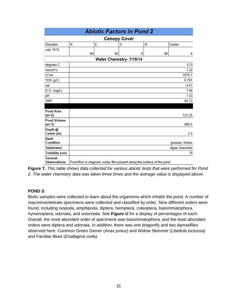
The abiotic factors that influence this pond can be found in Figure T below. Data was collected

for canopy cover, water chemistry, pond area and volume, depth at center, bank condition,

substrate type, and turbidity. General observations were also recorded for this pond. Canopy

cover was most prominent on the west, east and north sides of the pond, with 90%, 85% and

80% cover, respectively. Meanwhile the south end of the pond had 0% canopy cover. The area

of this pond was measured at roughly 722.25 meters squared. The volume of Pond 2 was

measured at 600.5 meters cubed, with a center depth of 2.4 meters. Primarily grasses and

forbes surround the banks of Pond 2. The turbidity measured at 70 centimeters, with pond

substrates consisting of algae and branches. The temperature of Pond 2 was 12.9 degrees

Celsius. The pH was 7.43. It was also observed that this pond’s water flow was stagnant, with a

sudsy film present along the surface of the pond. Dissolved oxygen was slightly lower in Pond 2,

with a measurement of 7.66 mg/L.

31

Figure T. This table shows data collected for various abiotic tests that were performed for Pond

2. The water chemistry data was taken three times and the average value is displayed above.

POND 3:

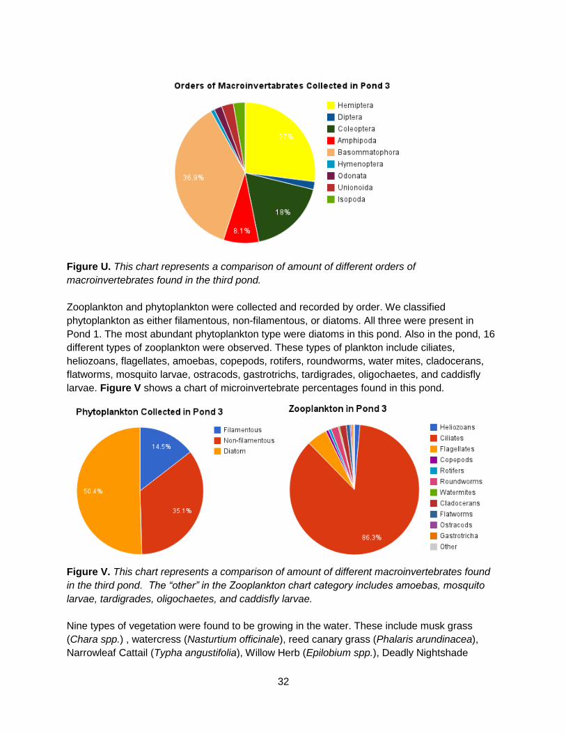
Biotic samples were collected to learn about the organisms which inhabit the pond. A number of

macroinvertebrate specimens were collected and classified by order. Nine different orders were

found, including isopoda, amphipoda, diptera, hemiptera, coleoptera, basommatophora,

hymenoptera, odonata, and unionoida. See Figure U for a display of percentages of each.

Overall, the most abundant order of specimens was basommatophora, and the least abundant

orders were diptera and odonata. In addition, there was one dragonfly and two damselflies

observed here: Common Green Darner (Anax junius) and Widow Skimmer (Libellula luctuosa)

and Familiar Bluet (Enallagma civile).

32

Figure U. This chart represents a comparison of amount of different orders of

macroinvertebrates found in the third pond.

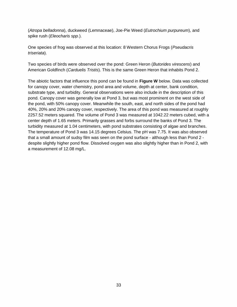
Zooplankton and phytoplankton were collected and recorded by order. We classified

phytoplankton as either filamentous, non-filamentous, or diatoms. All three were present in

Pond 1. The most abundant phytoplankton type were diatoms in this pond. Also in the pond, 16

different types of zooplankton were observed. These types of plankton include ciliates,

heliozoans, flagellates, amoebas, copepods, rotifers, roundworms, water mites, cladocerans,

flatworms, mosquito larvae, ostracods, gastrotrichs, tardigrades, oligochaetes, and caddisfly

larvae. Figure V shows a chart of microinvertebrate percentages found in this pond.

Figure V. This chart represents a comparison of amount of different macroinvertebrates found

in the third pond. The “other” in the Zooplankton chart category includes amoebas, mosquito

larvae, tardigrades, oligochaetes, and caddisfly larvae.

Nine types of vegetation were found to be growing in the water. These include musk grass

(Chara spp.) , watercress (Nasturtium officinale), reed canary grass (Phalaris arundinacea),

Narrowleaf Cattail (Typha angustifolia), Willow Herb (Epilobium spp.), Deadly Nightshade

33

(Atropa belladonna), duckweed (Lemnaceae), Joe-Pie Weed (Eutrochium purpureum), and

spike rush (Eleocharis spp.).

One species of frog was observed at this location: 8 Western Chorus Frogs (Pseudacris

triseriata).

Two species of birds were observed over the pond: Green Heron (Butorides virescens) and

American Goldfinch (Carduelis Tristis). This is the same Green Heron that inhabits Pond 2.

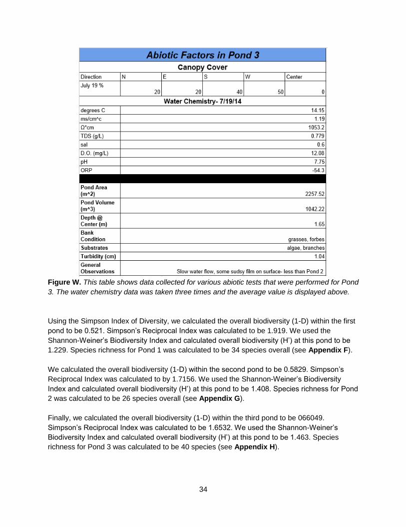
The abiotic factors that influence this pond can be found in Figure W below. Data was collected

for canopy cover, water chemistry, pond area and volume, depth at center, bank condition,

substrate type, and turbidity. General observations were also include in the description of this

pond. Canopy cover was generally low at Pond 3, but was most prominent on the west side of

the pond, with 50% canopy cover. Meanwhile the south, east, and north sides of the pond had

40%, 20% and 20% canopy cover, respectively. The area of this pond was measured at roughly

2257.52 meters squared. The volume of Pond 3 was measured at 1042.22 meters cubed, with a

center depth of 1.65 meters. Primarily grasses and forbs surround the banks of Pond 3. The

turbidity measured at 1.04 centimeters, with pond substrates consisting of algae and branches.

The temperature of Pond 3 was 14.15 degrees Celsius. The pH was 7.75. It was also observed

that a small amount of sudsy film was seen on the pond surface - although less than Pond 2 -

despite slightly higher pond flow. Dissolved oxygen was also slightly higher than in Pond 2, with

a measurement of 12.08 mg/L.

34

Figure W. This table shows data collected for various abiotic tests that were performed for Pond

3. The water chemistry data was taken three times and the average value is displayed above.

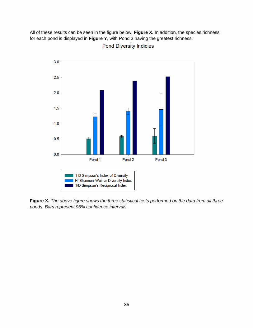
Using the Simpson Index of Diversity, we calculated the overall biodiversity (1-D) within the first

pond to be 0.521. Simpson’s Reciprocal Index was calculated to be 1.919. We used the

Shannon-Weiner’s Biodiversity Index and calculated overall biodiversity (H’) at this pond to be

1.229. Species richness for Pond 1 was calculated to be 34 species overall (see Appendix F).

We calculated the overall biodiversity (1-D) within the second pond to be 0.5829. Simpson’s

Reciprocal Index was calculated to by 1.7156. We used the Shannon-Weiner’s Biodiversity

Index and calculated overall biodiversity (H’) at this pond to be 1.408. Species richness for Pond

2 was calculated to be 26 species overall (see Appendix G).

Finally, we calculated the overall biodiversity (1-D) within the third pond to be 066049.

Simpson’s Reciprocal Index was calculated to be 1.6532. We used the Shannon-Weiner’s

Biodiversity Index and calculated overall biodiversity (H’) at this pond to be 1.463. Species

richness for Pond 3 was calculated to be 40 species (see Appendix H).

35

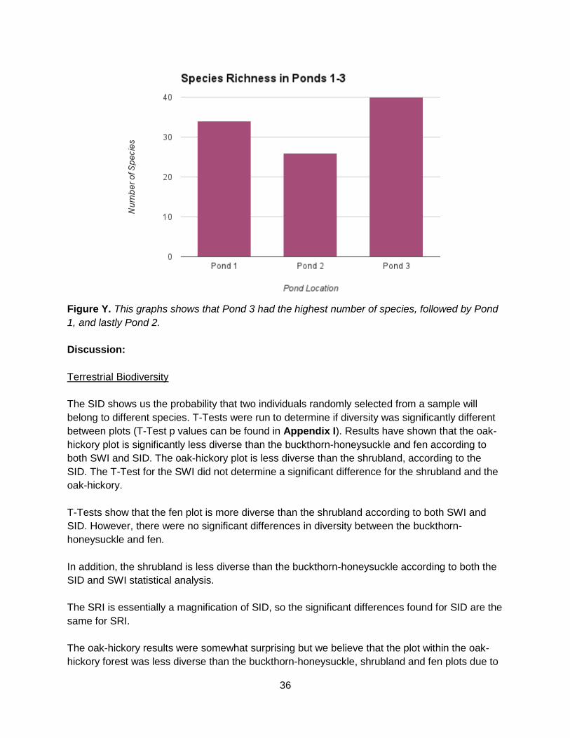
All of these results can be seen in the figure below, Figure X. In addition, the species richness

for each pond is displayed in Figure Y, with Pond 3 having the greatest richness.

Figure X. The above figure shows the three statistical tests performed on the data from all three

ponds. Bars represent 95% confidence intervals.

36

Figure Y. This graphs shows that Pond 3 had the highest number of species, followed by Pond

1, and lastly Pond 2.

Discussion:

Terrestrial Biodiversity

The SID shows us the probability that two individuals randomly selected from a sample will

belong to different species. T-Tests were run to determine if diversity was significantly different

between plots (T-Test p values can be found in Appendix I). Results have shown that the oak-

hickory plot is significantly less diverse than the buckthorn-honeysuckle and fen according to

both SWI and SID. The oak-hickory plot is less diverse than the shrubland, according to the

SID. The T-Test for the SWI did not determine a significant difference for the shrubland and the

oak-hickory.

T-Tests show that the fen plot is more diverse than the shrubland according to both SWI and

SID. However, there were no significant differences in diversity between the buckthorn-

honeysuckle and fen.

In addition, the shrubland is less diverse than the buckthorn-honeysuckle according to both the

SID and SWI statistical analysis.

The SRI is essentially a magnification of SID, so the significant differences found for SID are the

same for SRI.

The oak-hickory results were somewhat surprising but we believe that the plot within the oak-

hickory forest was less diverse than the buckthorn-honeysuckle, shrubland and fen plots due to

37

a lack of forest structural complexity. We believe that structurally diverse and well-developed

forest habitats consisting of dense understory, midstory and canopy strata generally harbor

more species than forests with simple structure. A forest with habitat complexity provides more

niches and different types of nesting and foraging resources for more species (MacArthur and

MacArthur 1961). In the oak-hickory test plot, a low number of plant species were observed,

with many of the species present found to be invasive. This forest stand was also not very

structurally diverse, with only canopy and understory layers observed. The combination of a lack

of structural complexity and native plant species diversity is the likely cause of the plot’s low

diversity compared to the other three ecosystems tested.

The difference in diversity in the oak-hickory and shrubland may or may not be significant

because of conflicting T-Test results from SID and SWI. This leads us to infer that the difference

in diversity between these two plots is less than the difference in diversity between any other

two plots.

We think the fen is more diverse than the shrubland because of the disturbance of intermittent

flooding in the fen. This hydrologic disturbance may increase herbaceous plant diversity, which

might lead to increased overall diversity. In contrast, the only disturbance to the shrubland is

precipitation. In addition, the fen may be significantly more diverse than we calculated because

we could not sample ground-dwelling invertebrates with pitfall traps because of the wet

environment in the fen. In addition, habitats in the presence of water tend to have higher

biodiversity than dry habitats.

It is possible that the buckthorn-honeysuckle is more diverse than the shrubland because of the

structural diversity created by the high species richness of herbaceous plants, the sapling

canopy created by the buckthorn and honeysuckle, as well as the presence of overstory trees.

Since the buckthorn-honeysuckle area used to be a wetland, the hydrology and soil condition

differs greatly from the shrubland and may promote higher biodiversity. In addition, the distance

to edge for this plot was only 3 m from a different habitat, thus suggesting an edge effect and

therefore a potential for higher biodiversity.

For abiotic factors, there was a significant change in pH from the dates tested. The pH

decreased for each plot on the second date that it was sampled. This is because we changed

testing kits for the second date. It was noted that the soil chemistry kit that we had originally

been using LaMotte Soil Testing Kit (Code 5928) was not reliable and therefore we used the

hand soil tester in the field (Kelway Soil Tester). The results for the buckthorn-honeysuckle plot

and the fen changed significantly because the peat that exists as soil did not settle when we did

the original soil test. The most reliable data is the results from July 15 in which we used the

Kelway Soil Tester. Unfortunately, in addition to not being able to use the pH results from the

LaMotte Soil Testing Kit (Code 5928), we do not believe the phosphorous (lb/a), potassium

(lb/a) or nitrogen (lb/a) to be significant or reliable for each of the four terrestrial plots.

Using the most reliable pH data collected July 15th, the buckthorn-honeysuckle and fen plots

have the lowest pH observed, as expected. The plot that was chosen within the buckthorn

38

ecosystem used to be a portion of the calcareous fen prior to invasion. The buckthorn plot and

the fen had lower pH (6 and 5.8 respectively) than the oak hickory and shrubland plots (both

6.4). Fens tend to be low in pH naturally, thus these results were expected.

There was also a change in the dissolved oxygen (DO) levels in the fen on the two dates that

samples were taken. This is most likely because the water levels in the fen differ daily because

of amount of precipitation. On June 19, the DO level was higher because there was more water

(more precipitation). On July 11, the DO level was lower because there was less precipitation

during that time period.

Across all four test plots, flora richness had a positive correlation with increasing leaf litter

percent composition, with the exception of the shrubland plot. This plot demonstrated an

anomaly of containing the highest species richness of all four test plots, despite also containing

the lowest leaf litter composition. The general trend of higher species richness with higher leaf

litter composition was expected across the four plots because more leaf litter contributes to

more organic matter and nutrient availability in the soil. This then allows for more plant species

which require a variety of nutrients and/or high-moderate nutrient amounts to survive

successfully in a given habitat.

Aquatic Biodiversity

In order to understand biodiversity across the three ponds, 7 different biotic tests were carried

out. From the data collected, the Simpson Index of Diversity (SID) and the Shannon-Weiner

Biodiversity Index (SWI) were able to be calculated. Figure X shows these results, including the

Simpson Reciprocal Index (SRI). Figure Y shows the species richness of all three ponds.

Results showed that Pond 2 has less species than Pond 1, but Figure X illustrates that Pond 2

is more diverse than Pond 1. This may be due to the relative even distribution of species

abundance numbers in Pond 2 versus, the huge abundance of one or two species in Pond 1.

According to T-Tests performed on the data, Pond 1 data was significantly less diverse than

Pond 2 for both SWI and SID (T-Test p values can be found in Appendix I). However, there

was no significant difference in data between Pond 1 and Pond 3 for both SWI and SID. A T-

Test shows that Pond 2 data is significantly less diverse than Pond 3 for both SWI and SID as

well. Again, the SRI is essentially a magnification of SID, so the significant differences found for

SID are the same for SRI.

We believe that the reason Pond 1 is less diverse than Pond 2 is because Pond 1 is where

water first enters the ecosystem from groundwater. Hence, the water lacks nutrients, which the

subsequent ponds gain as photosynthesis and nitrogen fixation take place as the water moves

through. This also may explain why we found more diversity in Pond 3 compared to Pond 2.

(See diversity indices in Figure X).

There is an interesting result in for pH changes throughout the ponds that warrants discussion.

We would expect to see that the pH decreases as the water flows from Pond 1 to Pond 3. We

expect this because the water that flows into Pond 1 is from a calcareous fen, which are often

39

neutral or alkaline. As the water flows, we expect the pH to become more acidic. Instead we see

that the ponds become more basic. There may be a few explanations for this result. To obtain

the values, the YSI tool was used at three samples were taken on one date and the numbers

were averaged. More repetition of this method, especially on different dates, would have

provided for more reliable results. In addition, the depth of the ponds increases from Pond 1 to

Pond 3, and the pH was tested at the very bottom of the ponds. pH could be higher at greater

depths for these ponds. However, we believe that simply more repetition at different areas of the

ponds would provide significantly more reliable results.

There were correlations between pond biodiversity and present abiotic factors. First of all, as the

volume of each pond increased, more biodiversity was observed. This was expected because

higher volume suggests more potential habitat and specific niches for organisms to inhabit.

Secondly, there tended to be more canopy cover (and thus less light) surrounding Ponds 1 & 2

compared to Pond 3. This was also expected because less canopy cover would allow for more

photosynthetic organisms to thrive and in turn would promote more viable habitat for

consumers. Thirdly, temperature increased as biodiversity increased. This was also expected

because of the amount of light that penetrates each pond. Finally, total dissolved solids (TDS)

showed a general increase across each pond. The amount of organic matter and biota

increases with the ponds as the water travels from 1 to 3, so we expected to see an increase of

TDS.

Conclusion: The above multi-taxon data coupled with abiotic measurements provides a

description of the species assemblages and the community structure of the four ecosystem

types chosen at the Loyola University Retreat and Ecology Campus using specific standardized

protocols. Many resident organisms were excluded by the specific sampling protocols used. For

instance, residence of smaller microhabitats or nocturnal species of bats and flying insects were

missed. Nevertheless, we have provided necessary baseline data that hopefully future

researchers and LUREC land managers can use alone or with other regional datasets to detect

changes either due to 1) alterations from restoration activities or 2) climate change. We also

hope that this research may be useful for predicting future trends as well.

Acknowledgements: Special thanks are extended to Dr. Roberta Lammers-Campbell for her

assistance in plant identification and various textual resources. Thanks to David Treering for

access to ArcGIS for our project. Thanks to Erin O’Connell for assistance with avian

identification in the field. In particular, thanks to the wonderful staff at LUREC. Financial support

was provided as a biodiversity internship by the Institute of Environmental Sustainability, Loyola

University Chicago, and a grant from the Northern Trust.

References:

Balaban, J., & Balaban, J. (2012) Common Spiders of the Chicago Region. Retrieved June 1,

2014, from http://fm2.fieldmuseum.org/plantguides/guide_pdfs/390.pdf

40

Borror, D., & White, R. (1958) A field guide to the insects of America north of Mexico. Boston:

Houghton Mifflin.

Borror, D., & White, R. (1970) A field guide to insects: America north to Mexico. Boston:

Houghton Mifflin.

Bouchard, R., & Ferrington, L. (2004) Guide to aquatic invertebrates of the upper midwest:

Identification manual for students, citizen monitors, and aquatic resource professionals. St.

Paul, Minn.: University of Minnesota.

Bryophytes: Illinois Bryophytes. (2006) Retrieved July 23, 2014, from

http://bryophytes.plant.siu.edu/PDFiles/Bryo-poster 1.pdfMosses. (Vol. 27). New York: Oxford

Univ Press.

Castner, J. (2000) Photographic atlas of entomology and guide to insect identification.

Gainesville, FL, USA: Feline Press.

Chu, H. (1949) How to know the immature insects. Dubuque Iowa: W.C. Brown.

Dichotomous Key for Protozoa. Retrieved July 1, 2014, from

http://hs.hastings.k12.mn.us/sites/6e3486ea-9f8c-4b52-bae2-

7be334b7418e/uploads/Dichotomous_Key_for_Protists.pdf

Duffie, P., Heememan, C., Jokinen, D., Kroll, W., Lammers-Campbell, R., & Morgan, R. (2012)

Protoctista, (a.k.a. Protists). In General Biology Laboratory manual. Chicago: Cengage

Learning.

Eaton, E., & Kaufman, K. (2007) Kaufman field guide to insects of North America. New York,

N.Y.: Houghton Mifflin.

Eddy, S., & Hodson, A. (1961) Taxonomic keys to the common animals of the North Central

States, exclusive of the parasitic worms, insects, and birds, (Revised/Expanded ed.).

Minneapolis: Burgess Pub.

Flora of North America Editorial Committee. (2007) Flora of North America: North of Mexico,

Key to Common Macroinvertabrates. (2014) Retrieved July 1, 2014, from

http://www.dec.ny.gov/docs/administration_pdf/lppondidentifykey.pdf

LaMotte Company. (2014) Soil Macronutrients Testing Kit, Order Code #5928-01, Ordering

information: http://www.fishersci.com

41

Mahan C., Sullivan, K., Kim, K., Yahner, R., & Abrams, M. (1998) “Ecosystem Profile

Assessment of Biodiversity: Sampling Protocols and Procedures”, U.S. Department of Interior

and the National Park Service.

MacArthur, R.H & MacArthur, J. (1961) On Bird Species Diversity. Ecology Vol. 42, No. 3, pp.

594-598.

Merritt, R. (2008) An introduction to the aquatic insects of North America: Includes color plates

and CD with interactive key (Revised/Expanded ed.). Dubuque, Iowa: Kendall Hunt.

Perez, E., & Mitten, S. (2012) Avian Species Structure at Loyola University Retreat and Ecology

Campus during the 2012 Summer Breeding Season. Loyola University Chicago.

https://www.yumpu.com/en/document/view/16446098/avian-species-structure-at-lurec-loyola-

university-chicago

Petrides, G. (1986) A field guide to trees and shrubs: Northeastern and north-central United

States and southeastern and south-central Canada (Revised/Expanded ed.). Boston: Houghton

Mifflin.

Simpsons Diversity Index. (2004) Retrieved August 1, 2014.

Smith, K., & Fernando, C. (1978) A guide to the freshwater calanoid and cyclopoid copepod

crustacea of Ontario. Waterloo, Ont.: Dept. of Biology, University of Waterloo.

Torke, B. (1974) An illustrated guide to the identification of the planktonic crustacea of Lake

Michigan,. Milwaukee: Center for Great Lakes Studies, University of Wisconsin.

Walker, D., & Van Egmond, W. (2000) November 1. Guide to Identification of Fresh Water

Microorganisms. Retrieved July 1, 2014, from

http://www.msnucleus.org/watersheds/mission/plankton.pdf

YSI Inc./Xylem Inc. (2013) YSI Model 556 Multi-Probe System (MPS), Code #556, Ordering

information: bsimpkiss@ysi.com, kwaits@ysi.com.

42

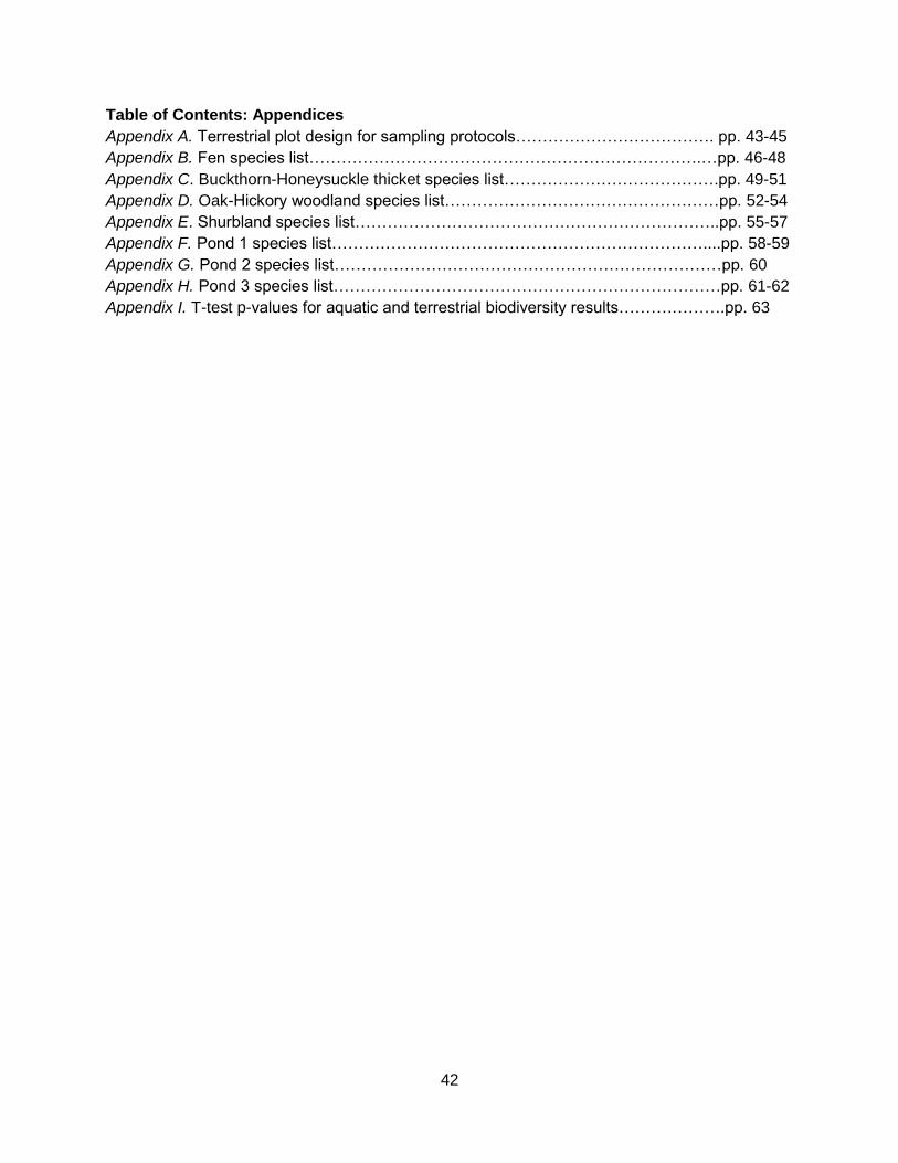
Table of Contents: Appendices

Appendix A. Terrestrial plot design for sampling protocols………………………………. pp. 43-45

Appendix B. Fen species list……………………………………………………………….…pp. 46-48

Appendix C. Buckthorn-Honeysuckle thicket species list………………………………….pp. 49-51

Appendix D. Oak-Hickory woodland species list……………………………………………pp. 52-54

Appendix E. Shurbland species list…………………………………………………………..pp. 55-57

Appendix F. Pond 1 species list……………………………………………………………....pp. 58-59

Appendix G. Pond 2 species list………………………………………………………………pp. 60

Appendix H. Pond 3 species list………………………………………………………………pp. 61-62

Appendix I. T-test p-values for aquatic and terrestrial biodiversity results……….……….pp. 63

43

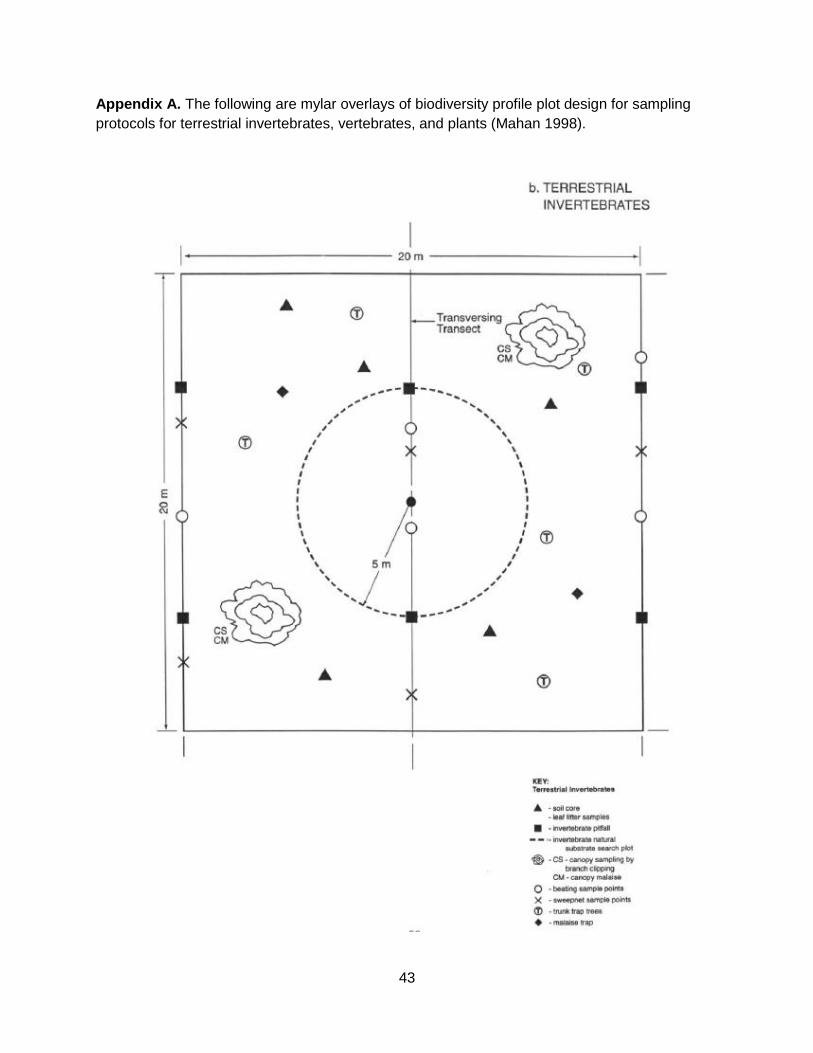
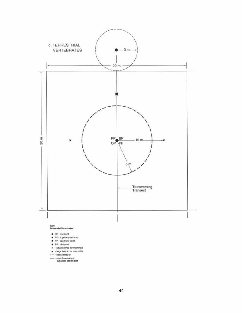
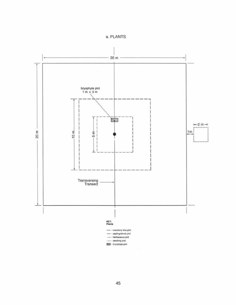
Appendix A. The following are mylar overlays of biodiversity profile plot design for sampling

protocols for terrestrial invertebrates, vertebrates, and plants (Mahan 1998).

44

45

46

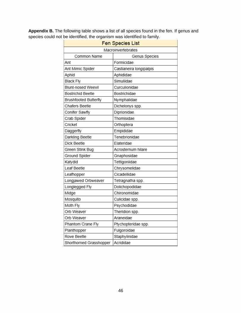
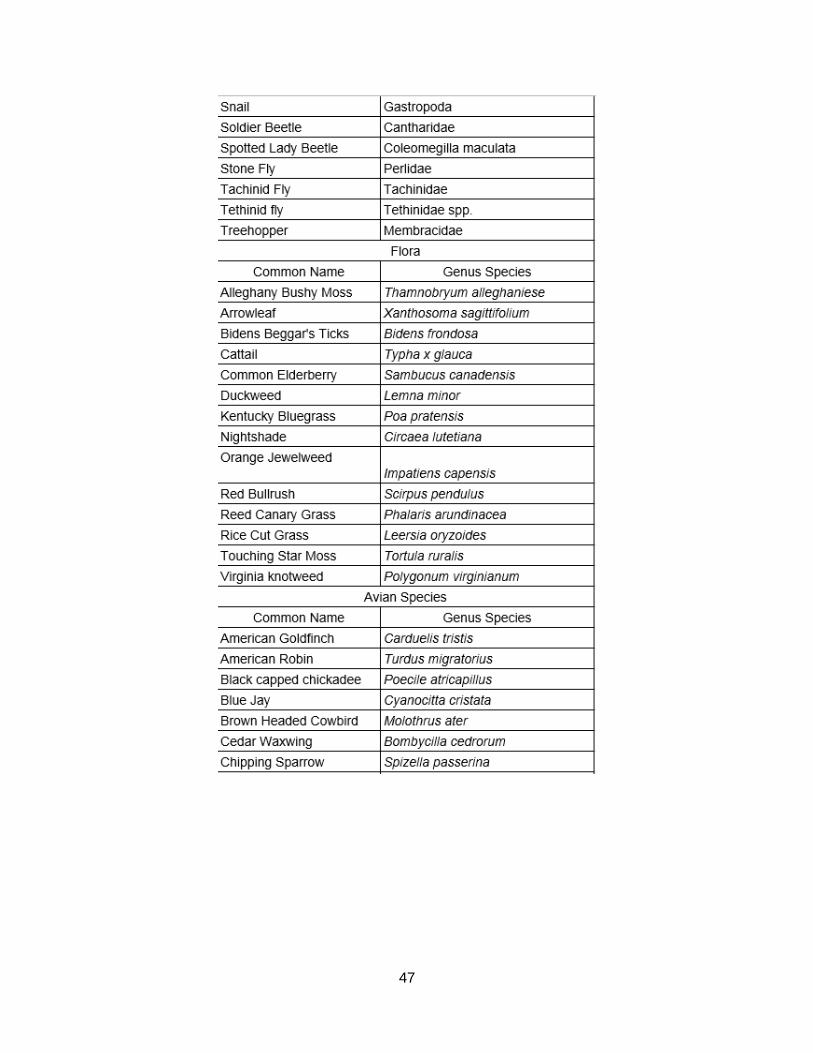
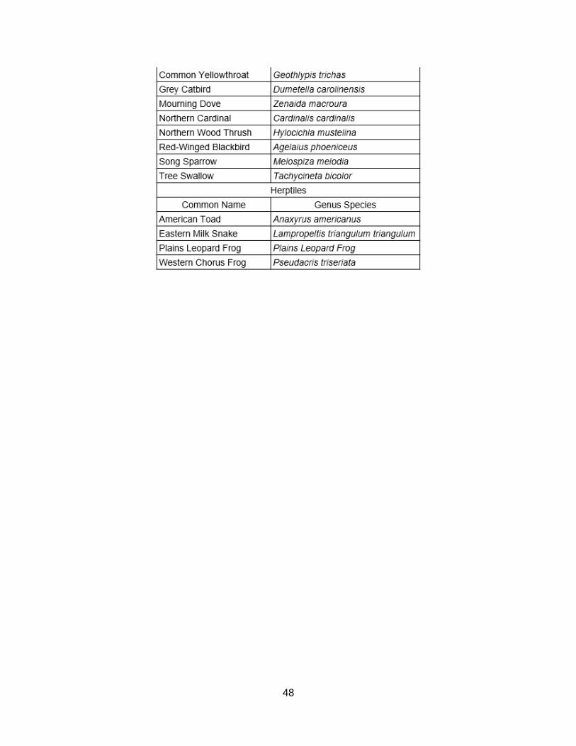
Appendix B. The following table shows a list of all species found in the fen. If genus and

species could not be identified, the organism was identified to family.

47

48

49

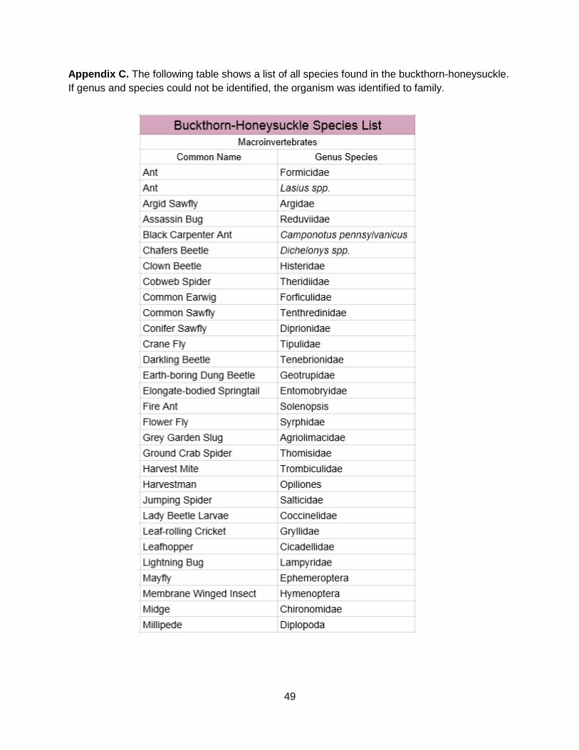
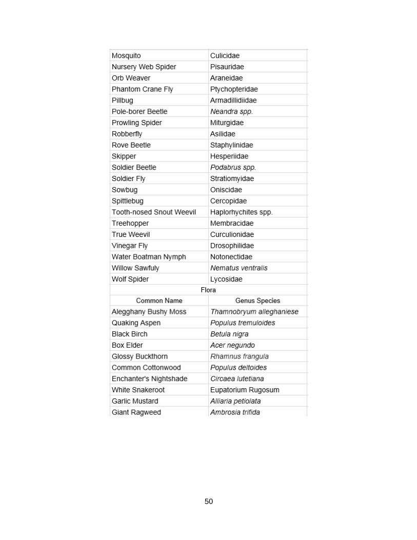
Appendix C. The following table shows a list of all species found in the buckthorn-honeysuckle.

If genus and species could not be identified, the organism was identified to family.

50

51

52

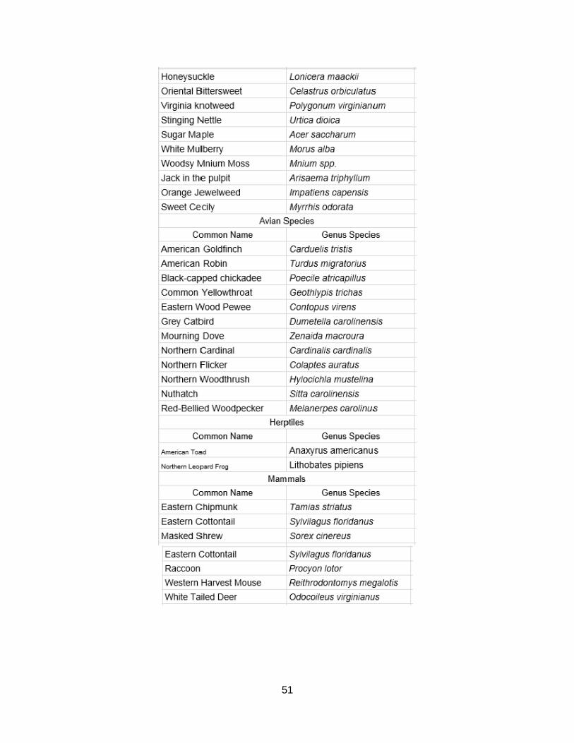
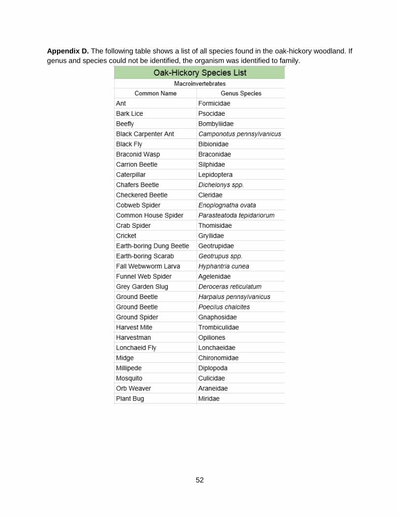
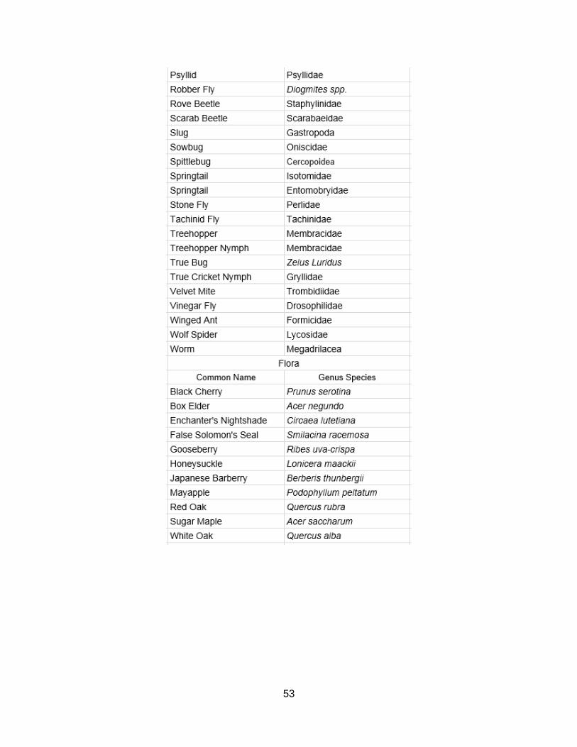
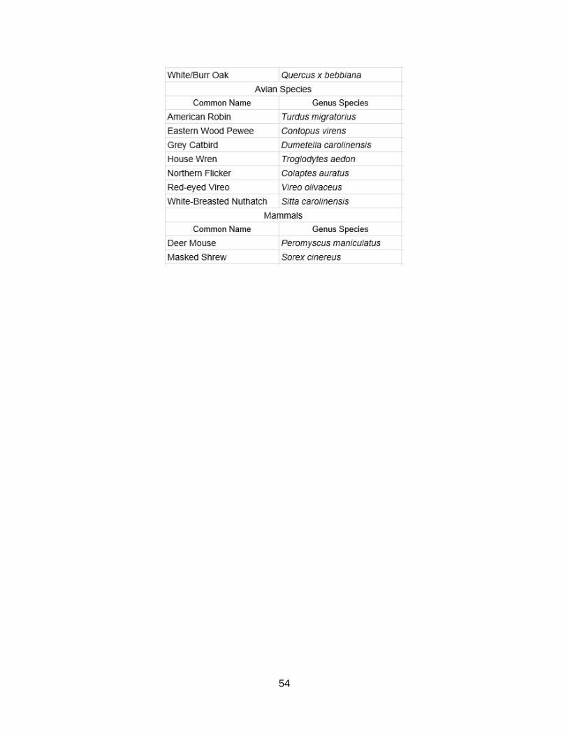
Appendix D. The following table shows a list of all species found in the oak-hickory woodland. If

genus and species could not be identified, the organism was identified to family.

53

54

55

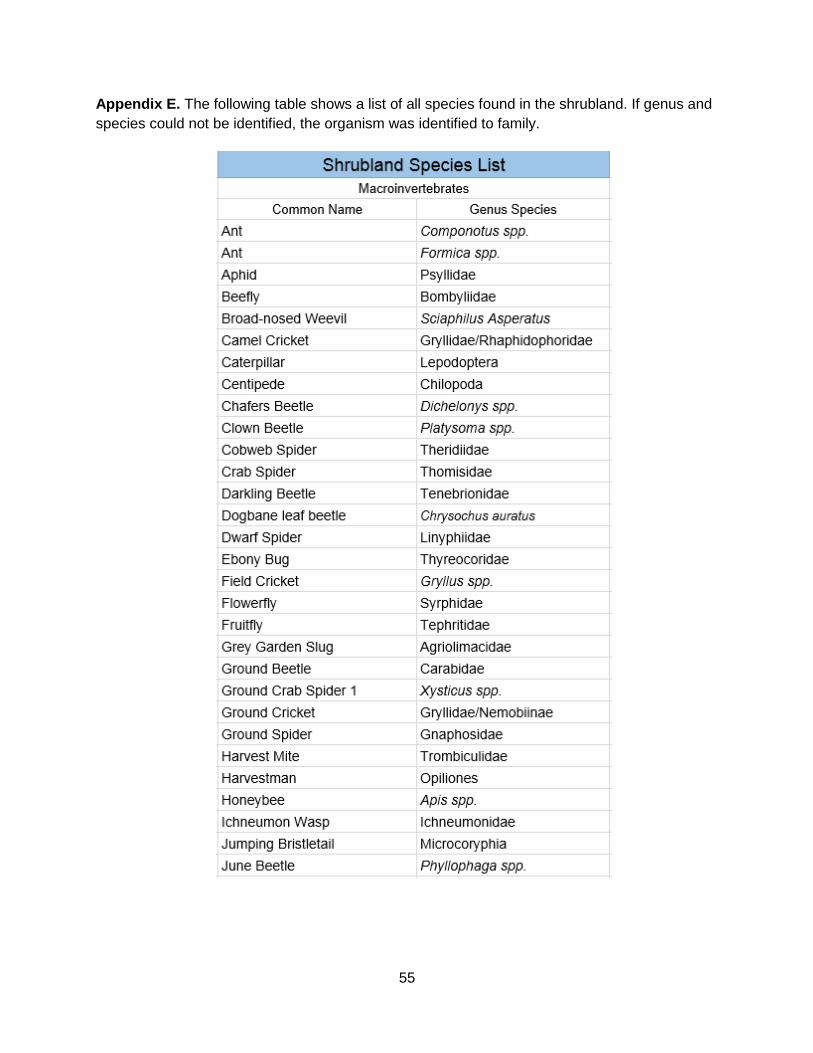
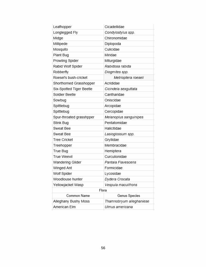
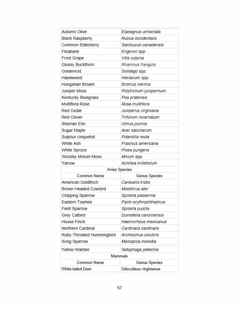
Appendix E. The following table shows a list of all species found in the shrubland. If genus and

species could not be identified, the organism was identified to family.

56

57

58

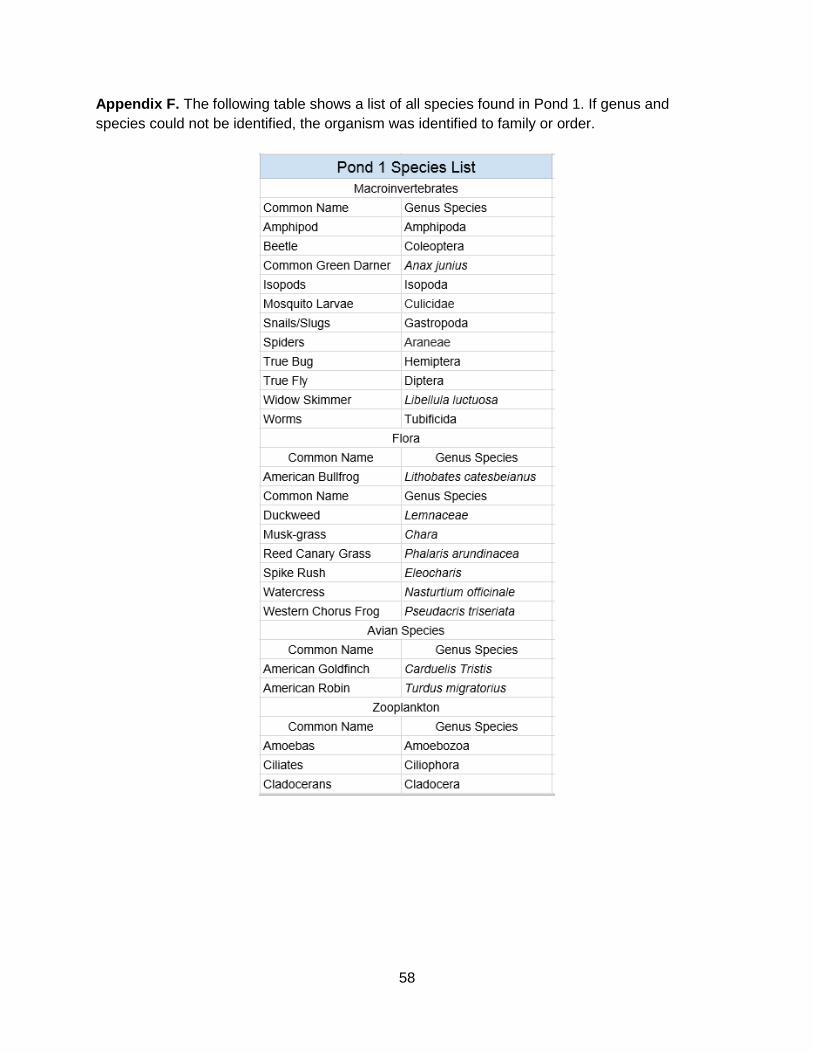
Appendix F. The following table shows a list of all species found in Pond 1. If genus and

species could not be identified, the organism was identified to family or order.

59

60

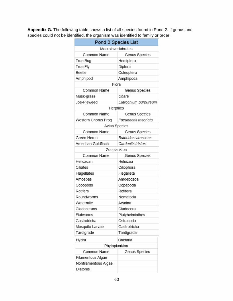
Appendix G. The following table shows a list of all species found in Pond 2. If genus and

species could not be identified, the organism was identified to family or order.

61

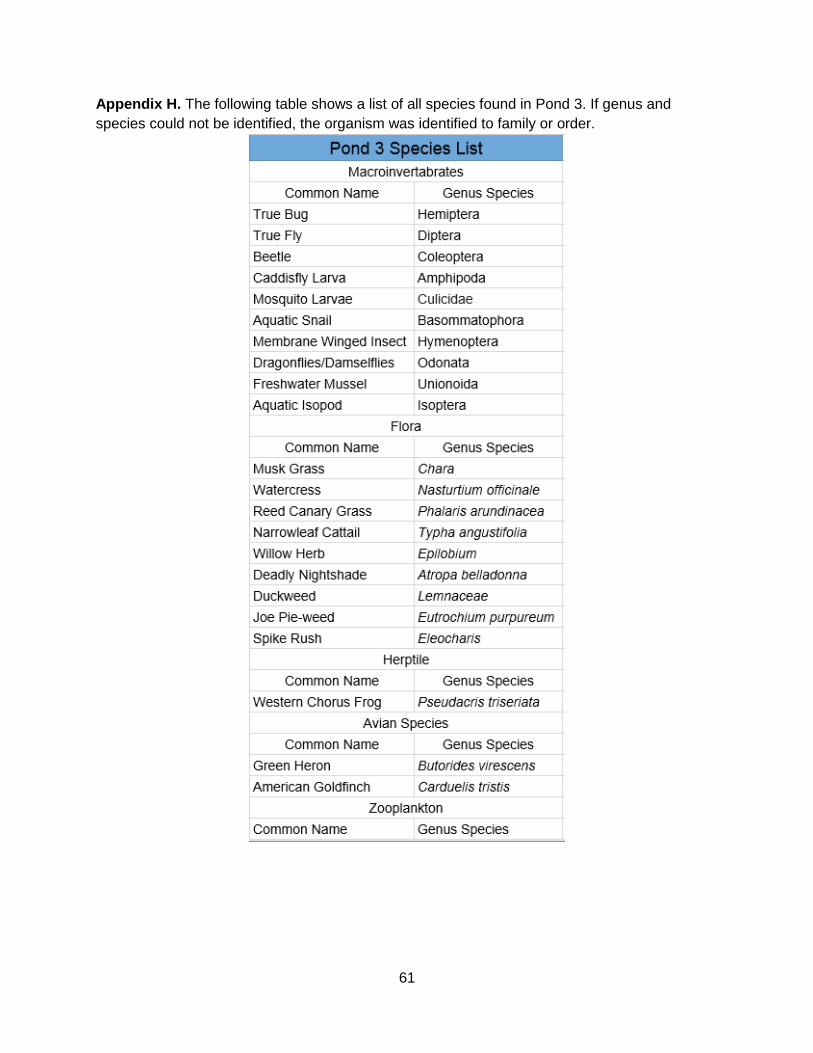
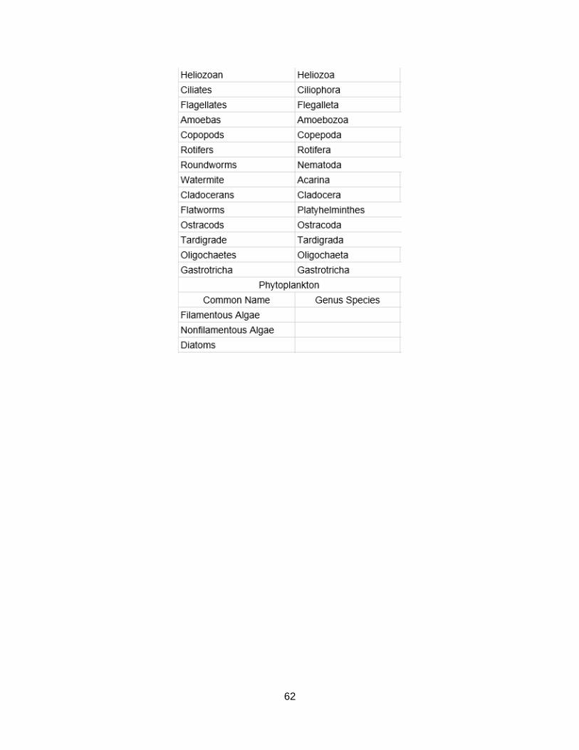
Appendix H. The following table shows a list of all species found in Pond 3. If genus and

species could not be identified, the organism was identified to family or order.

62

63

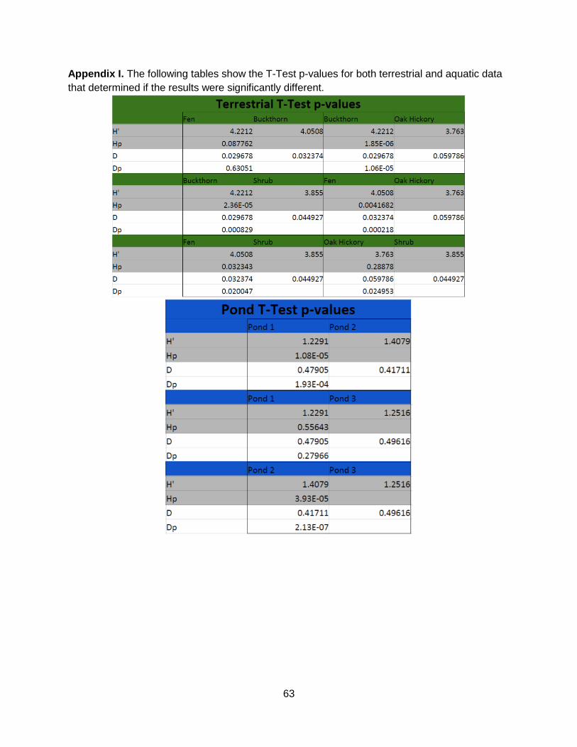
Appendix I. The following tables show the T-Test p-values for both terrestrial and aquatic data

that determined if the results were significantly different.