Economics Working Paper Series

2017/011

How much of a problem is problem gambling?

Rob Pryce, Ian Walker, and Rhys Wheeler

The Department of Economics Lancaster University Management School

Lancaster LA1 4YX UK

© Authors All rights reserved. Short sections of text, not to exceed

two paragraphs, may be quoted without explicit permission, provided that full acknowledgement is given.

LUMS home page: http://www.lancaster.ac.uk/lums/

0

How much of a problem is problem gambling? Rob Pryce*, Ian Walker+, and Rhys Wheeler‡

* ScHaRR, University of Sheffield

‡ Department of Economics, Lancaster University Management School

+ Department of Economics, Lancaster University Management School, and IZA Bonn

February 2017

Keywords: gambling, lotto, problem gambling, well-being JEL codes: I3, I31, D8 Abstract Problem gambling is conventionally defined by the score in a specific questionnaire exceeding some critical value and data suggests is that 0.7% of adults in the UK could be afflicted. However, the literature has not evaluated the size of the harm associated with such an affliction and this research evaluates the effect of problem gambling on self-reported well-being which, together with a corresponding effect of income on well-being, allows us to construct a money-metric of the (self) harm associated with being a problem gambler. Our estimates suggest that problem gambling imposes a very large reduction in individual well-being. Acknowledgements: We are grateful to the Gambling Commission, especially Ben Hader and James Holdaway, for advice and encouragement but the authors are solely responsible for the analysis, and the work in no way reflects the views of the Gambling Commission. The work was supported by an EU Framework 7 grant for the ALICE-RAP project - see http://www.alicerap.eu/, and by an ESRC CASE PhD studentship. The data was collected by NATCEN on behalf of the Gambling Commission and it was provided to us by the UK Data Service at Essex University. It is readily available to other researchers via www.UKDataservice.ac.uk. We would be happy to assist subsequent researchers and our own code is available from the corresponding author. David Forrest provided invaluable advice on the PG literature in general and on the lessons from his own PG research. Conversations with him greatly clarified our thinking about our IV strategy and the interpretation of our results. We are also grateful for valuable comments from Carolyn Downs, David Kang, Andrew Oswald, and Nick Powdthavee, and from seminar participants at Lancaster University, Sydney University, University of Wollongong, SFI Copenhagen, Leicester University, Temple University PA, and at the 2016 International Conference on Gambling and Risk Taking in Las Vegas.

Corresponding author: Professor Ian Walker, Department of Economics, Lancaster University, Lancaster LA1 4YX, UK. Email ian.walker@lancaster.ac.uk

1

1. Introduction

This research is concerned with evaluating the costs associated with being a “problem

gambler”. Problem gambling is usually defined by aggregating responses across questions

which are embedded within a screen. When administered to large samples of individuals this

facilitates an estimate of the prevalence of problem gambling. An individual is then defined

as a problem gambler (PG=1) if that individual’s score on the screen exceeds some critical

value. There are several such screens used in this literature and they each contain questions

that are designed to detect behaviour associated with pathological gambling and/or gambling

harms. Our estimate for the UK, that there are perhaps around ⅓ m of 46m UK adults who

are assessed to be problem gamblers is typical of the literature. However, none of the

extensive literature that attempts to quantify the prevalence of problem gambling has

attempted to also quantify the costs that problem gambling imposes on the individuals

afflicted by it, and this is the main contribution of this paper. Our baseline estimate of the

aggregate loss in well-being associated with PG is in approximately £90 thousand per

problem gambler, or over £30 billion pa across the population as a whole – a figure that is the

same order of magnitude as that often associated with alcohol abuse, and even exceeds

overall gambling expenditures1.

Gambling is an important part of many economies. Expenditure net of winnings

(sometimes referred to as Gross Gambling Yield, GGY) in the UK 2014/5 is close to £12

billion pa, or 0.6% of GNP; and overall expenditure is close to £50b or more then 2.5% of

GNP. Relative to other “sins”, gambling is typically not highly taxed; and taxes have been

driven downward as regulators and tax authorities have struggled with the increasingly

footloose nature of the industry that is becoming more highly dominated by online, and often

offshore, provision. Consumers in the UK do not directly pay tax on gambling - with the

exception of the products sold by the National Lottery, sales of which are taxed at 12% plus a

levy for “good causes” of approximately 28%. Other suppliers pay 15% on “profits”, defined

as revenue minus winnings2. The motivation for sin taxes is driven by the notion that

1 The Gambling Commission estimate of GGY (bets minus winnings) on gambling is £13.6b for 2015/15. HMRC reports tax revenue of £2.1 billion for 2014/15, and the Gambling Commission reports further good causes revenue from the National Lottery portfolio of games of £3.8 billion. The Institute of Alcohol Studies estimates of the harms associated with alcohol abuse in the UK is in the order of £21b pa. This estimate aggregates effects associated with crime, absenteeism, and health. The IAS reports results that include wider harms that aggregate to over £50b pa. Tax revenue from alcohol is approximately £10b p.a. 2 In the case of FOBTs (Fixed odds betting terminals), that are thought to be particularly likely to generate PG, the tax is 25%.

2

consumption causes harm that is not internalised. But these harms are often largely self-

inflicted, sometimes uncertain, and often long-term, in which case penal levels of tax need to

be motivated by other considerations associated with behavioural deficiencies in individual

preferences. Indeed, whether to legalise and tax the consumption of some commodities, as

opposed to criminalise, has been analysed by Becker et al (2006) who show that the demand

and supply elasticities as well as the nature of harms, play an important role in the optimal

design of policy. Thus, our contribution here speaks to one of the critical parameters relevant

to the design of public policy relevant to potentially harmful products.

Our analysis exploits the availability of data on well-being in a large household

sample survey. We construct a financial measure of PG by estimating the relationship

between subjective well-being, PG, and income. The methodology draws on the seminal

work on “happiness” and a particularly good early exemplar is Clarke and Oswald (2002).

The method effectively scales the effect of PG on well-being by the effect of income on well-

being to monetize the estimate of PG on well-being. This well-being approach is a catch-all

one – it looks, not at the mediating mechanisms, but directly at the effect on the well-being of

individuals, irrespective of how that comes about. The results are dramatic: our baseline

estimate is that the harm associated with PG is close to £100,000 pppa which, for ⅓ of a

million PGs, amounts to over £30 billion pa.

However, there are a number of threats to the legitimacy of the well-being

methodology that are typically not addressed in that literature. In particular, measurement

error and other sources of endogeneity are usually ignored by the simple regression method

that is used to obtain the statistical estimates. Measurement error in PG inevitably understates

the effect of PG on well-being.3 On the other hand, PG might be symptom of low well-being

rather than the other way around. This reverse causality is likely to bias the estimate of PG on

well-being upward. Since these biases counteract each other, it is unclear what the net effect

would be – the true effect might be larger or smaller than our baseline results.

We attempt to tackle these endogeneity issues head-on using an instrumental variables

(IV) approach. We find implausibly large estimates that suggest even larger losses in

aggregate well-being than our simple headline results – perhaps double what our baseline

3 To make things more complicated, measurement error in income is likely to understate the effect of income on well-being – and since it is used to scale the effect of PG on well-being this will tend to overstate the financial effect of the loss in well-being associated with PG.

3

estimates suggest. We would need a substantially larger dataset to come to any firm

conclusions. For the moment we treat our OLS estimates as a plausible benchmark.

An alternative approach to the investigation of well-being data would consider the

effect of PG on a list of all relevant mediators – for example, in the case of PG, researchers

may look at the effect on mental health, employment, wages (a measure of productivity in the

labour market) conditional on employment, tax receipts and welfare payments etc. The

predicted effects would then need to be “valued” and aggregated4. A recent UK example is

Thorley et al (2016) which focuses on those outcomes that affect some of the range of other

people and agencies, apart from the PG. That study, from IPPR, focuses on only certain

aspects of health, housing, crime, and welfare and employment, and provides estimates of a

cost of just £1.2b pa. This alternative methodology is likely to miss elements of the

transmission mechanism, perhaps because of limitations in the available data. This method is

also more likely to miss true externalities - effects of one person’s PG on other people (this is

not measured in the IPPR study, for example). The well-being method is less likely to be

affected by this – since it will capture the effects of own PG on other people to the extent that

the former feels altruistic towards the latter.5 In any event, the well-being method seems

likely to yield bigger estimates than the alternative to the extent that the latter embraces only

a subset of possible mediators.

Nonetheless, our own analysis is deficient in that it has no policy content over and

above highlighting the magnitude of the problem. To address how to ameliorate the problem

we need to uncover the transmission mechanism that links PG to (much lower) well-being.

The most obvious contenders are gambling expenditure and gambling losses and we attempt

quantify their role once we have established the magnitude of the problem. However, we can

see that gambling expenditure in our data is heavily underreported, with the exception of

scratchcards and lotto. Our finding of no effect of overall gambling spend on the impact that

PG has on well-being is likely to be a manifestation of the measurement error in the data.

However, we find that lotto are accurately measured in our data, we estimate that scratchcard

spending does have a statistically significant mediating role, but not the spending on lotteries. 4 An exhaustive report on the Australian gambling market by Delfabbro (2010) for the Australian Productivity Commission (APC) reviews the literature on a wide variety of harms associated with PG (ch 3) and comments on the APC’s own attempt (Australian Productivity Commission, 2010) to aggregate harms and compare with consumer surplus benefits (ch 6). 5 Our attempts to estimate the effects of PG on the well-being of spouses yielded small and imprecise estimates.

4

2. Related literature

There is a considerable literature on problem gambling. All of the quantitative work

uses one or more of a number of screens that consist of a set of questions that are thought to

be indicative of PG. An overview of the problem gambling literature is provided by Orford et

al (2003), which exploits the Gambling Prevalence Surveys (GPS) that pre-date the 2010

GPS used in our analysis. Griffiths provides an updated review of the British literature in

Griffiths (2014), which includes analysis of the 2010 GPS data used here, as well as

providing wider international comparisons. The British GPS is one of a small number of

random sample surveys of populations that have been conducted in the world for this purpose

– many samples elsewhere are drawn from specific subsets of the population. Indeed, Britain

has had three such surveys although the changes across years have been small and the

samples are not large enough to have the power to reject stability of the prevalence of

problem gambling across time. For the 2010 dataset used here Griffiths argues that

“…problem gambling in Great Britain is a minority problem that effects less than 1% of the

British population…”, and that “Problem gambling also appears to be less of a problem than

many other potentially addictive behaviours”6.

Related research does consider the public health consequences of gambling which

looks at specific outcomes in a piecemeal fashion. An excellent early overview is by Shaffer

and Korn (2002) which candidly confesses that the causal effect of gambling on adverse

outcomes such as mental health, crime, domestic violence, etc. cannot be distinguished from

the correlations, even though some of these correlations are large. Establishing that an effect

of gambling on any of these outcomes is causal is likely to be problematic. Establishing the

causal effect on all possible outcomes is likely to be considerably harder. The well-being

approach offers a practical and legitimate way of condensing the problem into a univariate

outcome.

However, none of the extensive PG literature that focusses on measuring the

prevalence of PG makes any attempt to uncover the size of the problem that PG generates for

those people who are afflicted. So this literature is seriously incomplete. Only Forrest (2016),

6 Here, Griffiths is referring to Sussman et al (2011) who surveyed the prevalence of other addictions and found that addictions to alcohol, cigarette smoking, illicit drugs, work, and shopping appear to have a prevalence rate of around 5% to 15% of the population.

5

who also uses the 2010 GPS that we employ in our own empirical work here, draws any

attention to this issue.7

The precise question asked in the GPS data was “Taking all things together, on a scale

of 1 to 10, how happy would you say you are these days?” Deaton and Stone (2013) refer to

measures of well-being such as that in the GPS as “evaluative” and they report that there is a

stable relationship in the literature between such evaluative measures of well-being and log

income, with a coefficient that is typically around ½ - implying that a 100% increase in

income would raise well-being by ½.8 The methodology estimates well-being regressions

using large random samples of individuals, and the relative coefficients of income and of the

life event in question are used to provide a financial ‘compensating amount’ for that event.

The method has been used to evaluate the effects of marital status, unemployment, health,

and many other phenomena.9

Forrest (2016) reports a large difference in mean well-being for PG vs non-PG

individuals in the GPS data10. He goes on to investigate the other correlates of well-being in

the 2010 GPS data, including income intervals and many other control variables. He reports

estimates that suggest that the effect of PG is strongly and significantly negative. While he

does not report the implied effect of income because of the grouped nature the data, he does

demonstrate that the effect of PG on W is comparable with the effect of divorce and

widowhood, relative to married. However, it seems likely that several of the control variables

that Forrest includes represent “bad controls”: variables that are themselves endogenous and

whose presence results in biased coefficients of the PG variable and/or those on income

7 While Forrest (2016) does not report the effect of problem gambling on well-being he does report that gambling that is not problematic increases well-being by 0.2 points, on the 1 to 10 scale. We fail to find a statistically significant effect in our specification using the same data. 8 If we interpreted the coefficient on log-income in the relationship between well-being and log income as a coefficient of a Constant Relative Risk Aversion (CRRA) expected utility function then it would be within the ballpark of estimates from other methodologies. For example, Hartley et al (2013) estimate the CRRA using a sample of gameshow players in an environment where players might win a wide range of amounts. Their well-determined estimate of risk aversion would be consistent with a coefficient on log income of 1. 9 Powdthavee and van den Berg (2011) use the well-being method to evaluate the effect of a variety of medical conditions on several measures of well-being. However, they do not consider the issues we raise above which are likely to bias the results in different ways for different well-being measures. An excellent review of the issues around the use of subjective well-being measures can be found in Nikilova (2016), albeit in the context of development. 10 Since 2010 the DSM and PGSI screens used in the GPS surveys have instead been incorporated in the Health Survey of England (HSE), which does not contain well-being questions.

6

intervals11. For example, education, income, employment, self-reported health, and marital

status are all arguably endogenous; and they are likely correlated with PG as well as with

income and well-being. It is unclear what the direction of bias associated with including such

bad controls would be on the PG or income coefficients.

In addition to the bad controls problem, which we address here, there are strong

grounds for thinking that PG itself is measured with error. It is, after all, self-reported and

individuals may wish to conceal their problem from the interviewer if not from themselves.

Moreover, PG itself, even if it is not subject to measurement error, is likely to be endogenous

because both PG and well-being may be correlated with some unobservable factors that are

not explicitly included in the modelling - for example, with non-cognitive traits such as self-

control. Or, PG might cause low well-being at the same time as low well-being causes PG.

Resolving this endogeneity issue is crucial for being able to put a causal interpretation to the

estimated relationship between PG and well-being in observational data. We need a causal

estimate of the effect of PG, rather than a simple correlation, since our objective is to obtain

estimates that will help policymakers understand the consequences of a policy-induced

change in PG.

Moreover, a common weakness of the existing literature is that income is typically

measured with error and this will tend to attenuate the coefficient on income in a well-being

equation. Since the money metric associated with the event in question will vary inversely

with the estimate of the effect of income on well-being this attenuation in the latter will

inflate the metric. Powdthavee (2010) appears to be the only paper to suggest how important

this problem is. He convincingly corrects for the measurement error in income, in the

relationship between income and well-being in the British Household Panel Study data, using

information on whether the interviewer saw the payslip of household members. Using this as

an instrumental variable for log income did indeed result in a large and statistically

significant increase in the estimated effect of log income.

A further concern relates to the idea of “rational addiction” pioneered by Becker and

Murphy (1988). They proposed a forward looking model of addiction where agents respond

to expected changes in future prices/costs as well as to current ones, and where current

consumption affects the marginal utility of future consumption. If this model were a true

11 The bad controls problem is discussed in section 3.2.3 of Angrist and Pischke (2009).

7

description of behaviour, and the well-being measure was an accurate metric of lifecycle

well-being, then we would expect to observe no well-being effect of PG.

The theory was widely criticised for not being able to explain the empirical

observation of the widespread regret expressed by addicts. In fact, this is not a valid criticism

of the theory – it is quite possible that addicts, once addicted feel currently worse of than they

would have been had they not decided originally that the discounted lifetime benefits exceed

the lifetime discounted costs. Moreover, extensions of the original theory, by Orphanides and

Zervos (1995) and Gruber and Koszegi (2001), allows for the possibility that individuals

experience imperfect foresight or time inconsistency over their potential to become addicted.

Individuals, in these extensions to the theory, still optimally make forward looking decisions

but are nonetheless allowed to ultimately regret those decisions because they may have

underestimated the ease with which they become addicted, or the present value costs of that

addiction.

Finally, the strong effect of PG on well-being begs the question of what mediating

factors are involved in the underlying transmission mechanism. Most evaluation work

focusses on the “total” effect of some “treatment”, rather than on the underlying “channels”

that drive the effect. Evaluation work does not usually investigate the possibility that the total

effect may be driven by specific channels that relate to “mediating” variables that affect the

final outcome. Here, we tentatively explore the role of gambling expenditures/losses and we

distinguish between draw-based lotto and scratchcard games–style games, and other forms of

gambling. It is not surprising, in the light of the lacuna around the magnitude of the harm that

PG implies, that the literature is again silent on the potential role that mediating factors might

play in determining this unknown magnitude. However, if we were able to establish the

mediation effects then we would at least be able to say something about the likely size of the

taxes that might be required to trigger the behavioural changes required since there is a (very

small) literature on gambling price elasticties – a literature that has recently been surveyed by

Frontier Economics (2014). Moreover, since the marketplace for gambling products is far

from being competitive it is difficult to resist the conclusion that the relatively concentrated

nature of supply, and the low marginal cost of the products supplied, would yield elasticities

that are probably close to -1. Given this, there are grounds for optimism that changes in the

structure of gambling taxation might be used to change behaviour to reduce harms. We

speculate in our concluding section about what might be required.

8

3. Data

Our dataset is the British Gambling Prevalence Survey (BGPS) 2010. An excellent

overview of the content and construction of the BGPS is provided by Wardle et al (2011).

BGPS contains two PG screens: DSM (Diagnostic and Statistical Manual of Mental

Disorders) IV and PGSI (Problem Gambling Severity Index)12. We focus our attention on the

DSM screen here because it has been used to make a very clear distinction between PG and

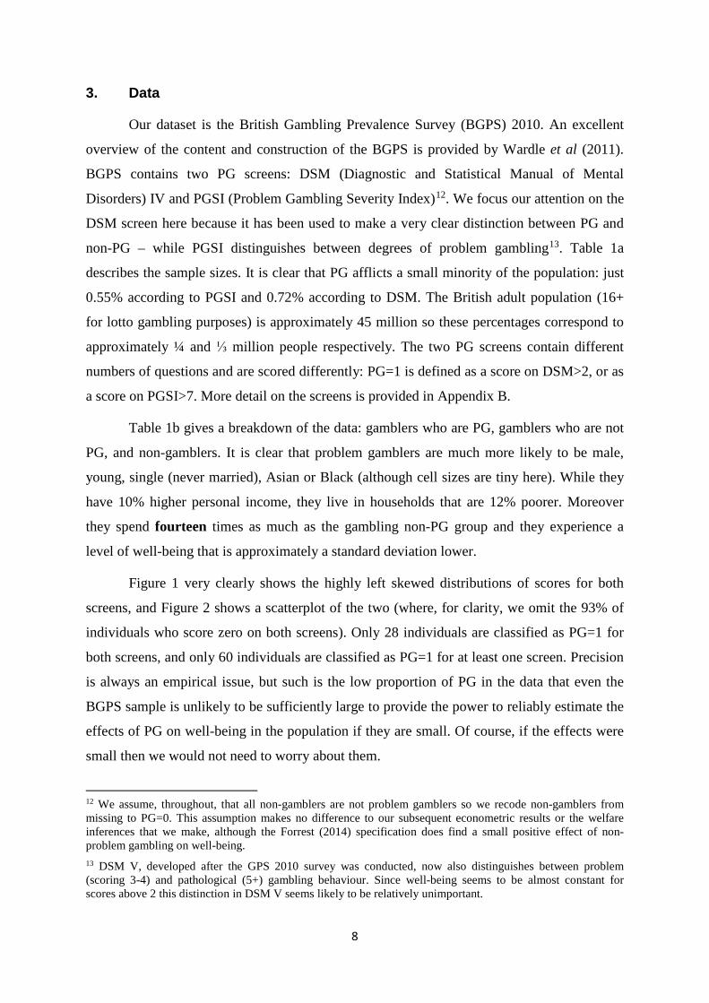
non-PG – while PGSI distinguishes between degrees of problem gambling13. Table 1a

describes the sample sizes. It is clear that PG afflicts a small minority of the population: just

0.55% according to PGSI and 0.72% according to DSM. The British adult population (16+

for lotto gambling purposes) is approximately 45 million so these percentages correspond to

approximately ¼ and ⅓ million people respectively. The two PG screens contain different

numbers of questions and are scored differently: PG=1 is defined as a score on DSM>2, or as

a score on PGSI>7. More detail on the screens is provided in Appendix B.

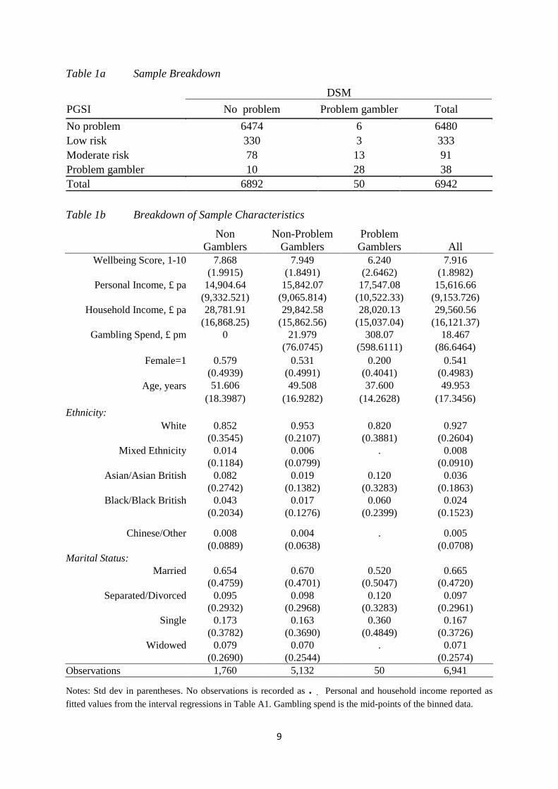
Table 1b gives a breakdown of the data: gamblers who are PG, gamblers who are not

PG, and non-gamblers. It is clear that problem gamblers are much more likely to be male,

young, single (never married), Asian or Black (although cell sizes are tiny here). While they

have 10% higher personal income, they live in households that are 12% poorer. Moreover

they spend fourteen times as much as the gambling non-PG group and they experience a

level of well-being that is approximately a standard deviation lower.

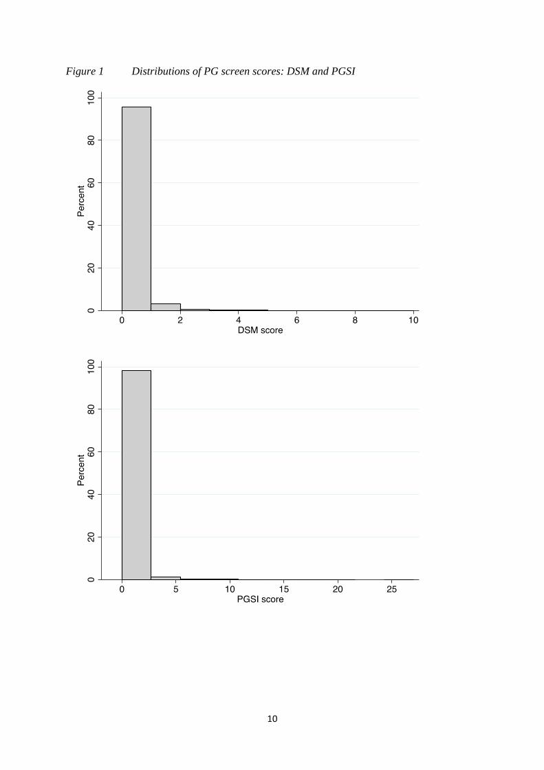
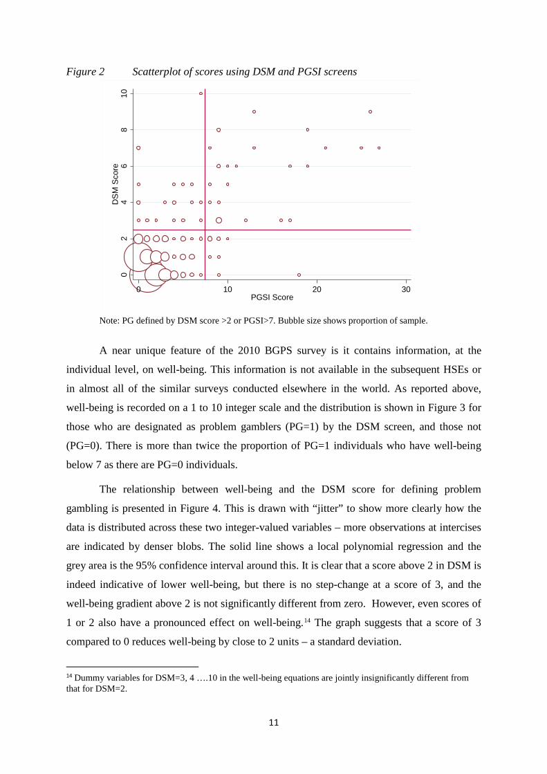
Figure 1 very clearly shows the highly left skewed distributions of scores for both

screens, and Figure 2 shows a scatterplot of the two (where, for clarity, we omit the 93% of

individuals who score zero on both screens). Only 28 individuals are classified as PG=1 for

both screens, and only 60 individuals are classified as PG=1 for at least one screen. Precision

is always an empirical issue, but such is the low proportion of PG in the data that even the

BGPS sample is unlikely to be sufficiently large to provide the power to reliably estimate the

effects of PG on well-being in the population if they are small. Of course, if the effects were

small then we would not need to worry about them.

12 We assume, throughout, that all non-gamblers are not problem gamblers so we recode non-gamblers from missing to PG=0. This assumption makes no difference to our subsequent econometric results or the welfare inferences that we make, although the Forrest (2014) specification does find a small positive effect of non-problem gambling on well-being. 13 DSM V, developed after the GPS 2010 survey was conducted, now also distinguishes between problem (scoring 3-4) and pathological (5+) gambling behaviour. Since well-being seems to be almost constant for scores above 2 this distinction in DSM V seems likely to be relatively unimportant.

9

Table 1a Sample Breakdown

DSM PGSI No problem Problem gambler Total No problem 6474 6 6480 Low risk 330 3 333 Moderate risk 78 13 91 Problem gambler 10 28 38 Total 6892 50 6942

Table 1b Breakdown of Sample Characteristics

Non

Gamblers Non-Problem

Gamblers Problem Gamblers

All

Wellbeing Score, 1-10 7.868 7.949 6.240 7.916 (1.9915) (1.8491) (2.6462) (1.8982)

Personal Income, £ pa 14,904.64 15,842.07 17,547.08 15,616.66 (9,332.521) (9,065.814) (10,522.33) (9,153.726)

Household Income, £ pa 28,781.91 29,842.58 28,020.13 29,560.56 (16,868.25) (15,862.56) (15,037.04) (16,121.37)

Gambling Spend, £ pm 0 21.979 308.07 18.467 (76.0745) (598.6111) (86.6464)

Female=1 0.579 0.531 0.200 0.541 (0.4939) (0.4991) (0.4041) (0.4983)

Age, years 51.606 49.508 37.600 49.953 (18.3987) (16.9282) (14.2628) (17.3456) Ethnicity:

White 0.852 0.953 0.820 0.927 (0.3545) (0.2107) (0.3881) (0.2604)

Mixed Ethnicity 0.014 0.006 . 0.008 (0.1184) (0.0799) (0.0910)

Asian/Asian British 0.082 0.019 0.120 0.036 (0.2742) (0.1382) (0.3283) (0.1863)

Black/Black British 0.043 0.017 0.060 0.024 (0.2034) (0.1276) (0.2399) (0.1523)

Chinese/Other 0.008 0.004 . 0.005 (0.0889) (0.0638) (0.0708) Marital Status:

Married 0.654 0.670 0.520 0.665 (0.4759) (0.4701) (0.5047) (0.4720)

Separated/Divorced 0.095 0.098 0.120 0.097 (0.2932) (0.2968) (0.3283) (0.2961)

Single 0.173 0.163 0.360 0.167 (0.3782) (0.3690) (0.4849) (0.3726)

Widowed 0.079 0.070 . 0.071 (0.2690) (0.2544) (0.2574) Observations 1,760 5,132 50 6,941

Notes: Std dev in parentheses. No observations is recorded as .. Personal and household income reported as fitted values from the interval regressions in Table A1. Gambling spend is the mid-points of the binned data.

10

Figure 1 Distributions of PG screen scores: DSM and PGSI

11

Figure 2 Scatterplot of scores using DSM and PGSI screens

Note: PG defined by DSM score >2 or PGSI>7. Bubble size shows proportion of sample.

A near unique feature of the 2010 BGPS survey is it contains information, at the

individual level, on well-being. This information is not available in the subsequent HSEs or

in almost all of the similar surveys conducted elsewhere in the world. As reported above,

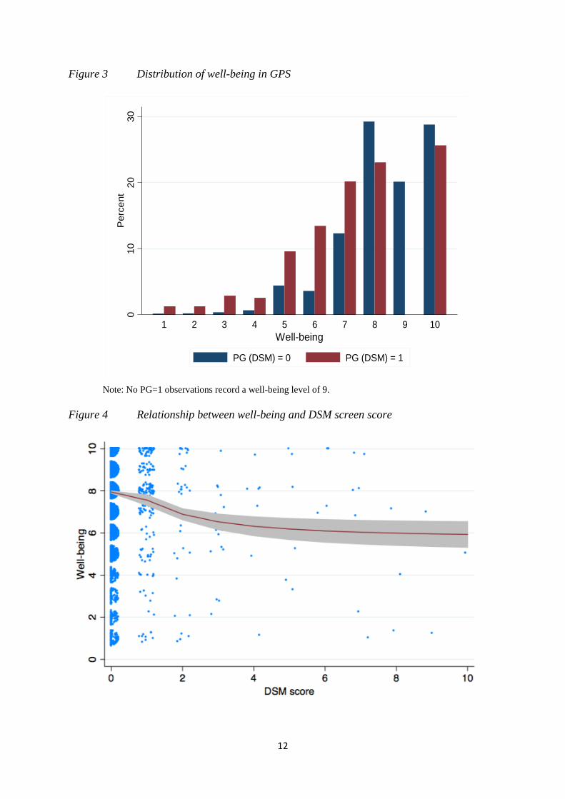
well-being is recorded on a 1 to 10 integer scale and the distribution is shown in Figure 3 for

those who are designated as problem gamblers (PG=1) by the DSM screen, and those not

(PG=0). There is more than twice the proportion of PG=1 individuals who have well-being

below 7 as there are PG=0 individuals.

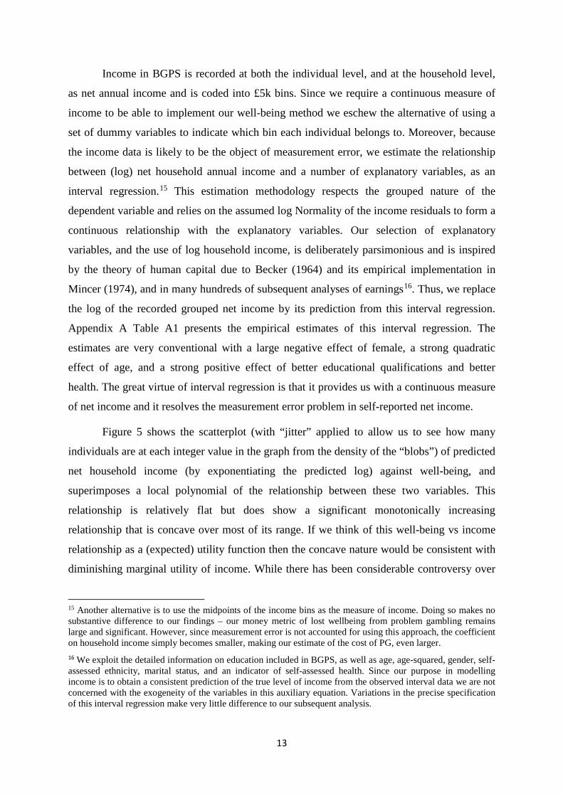
The relationship between well-being and the DSM score for defining problem

gambling is presented in Figure 4. This is drawn with “jitter” to show more clearly how the

data is distributed across these two integer-valued variables – more observations at intercises

are indicated by denser blobs. The solid line shows a local polynomial regression and the

grey area is the 95% confidence interval around this. It is clear that a score above 2 in DSM is

indeed indicative of lower well-being, but there is no step-change at a score of 3, and the

well-being gradient above 2 is not significantly different from zero. However, even scores of

1 or 2 also have a pronounced effect on well-being.14 The graph suggests that a score of 3

compared to 0 reduces well-being by close to 2 units – a standard deviation.

14 Dummy variables for DSM=3, 4 ….10 in the well-being equations are jointly insignificantly different from that for DSM=2.

02

46

810

DS

M S

core

0 10 20 30PGSI Score

12

Figure 3 Distribution of well-being in GPS

Note: No PG=1 observations record a well-being level of 9.

Figure 4 Relationship between well-being and DSM screen score

010

2030

Per

cent

1 2 3 4 5 6 7 8 9 10Well-being

PG (DSM) = 0 PG (DSM) = 1

13

Income in BGPS is recorded at both the individual level, and at the household level,

as net annual income and is coded into £5k bins. Since we require a continuous measure of

income to be able to implement our well-being method we eschew the alternative of using a

set of dummy variables to indicate which bin each individual belongs to. Moreover, because

the income data is likely to be the object of measurement error, we estimate the relationship

between (log) net household annual income and a number of explanatory variables, as an

interval regression.15 This estimation methodology respects the grouped nature of the

dependent variable and relies on the assumed log Normality of the income residuals to form a

continuous relationship with the explanatory variables. Our selection of explanatory

variables, and the use of log household income, is deliberately parsimonious and is inspired

by the theory of human capital due to Becker (1964) and its empirical implementation in

Mincer (1974), and in many hundreds of subsequent analyses of earnings16. Thus, we replace

the log of the recorded grouped net income by its prediction from this interval regression.

Appendix A Table A1 presents the empirical estimates of this interval regression. The

estimates are very conventional with a large negative effect of female, a strong quadratic

effect of age, and a strong positive effect of better educational qualifications and better

health. The great virtue of interval regression is that it provides us with a continuous measure

of net income and it resolves the measurement error problem in self-reported net income.

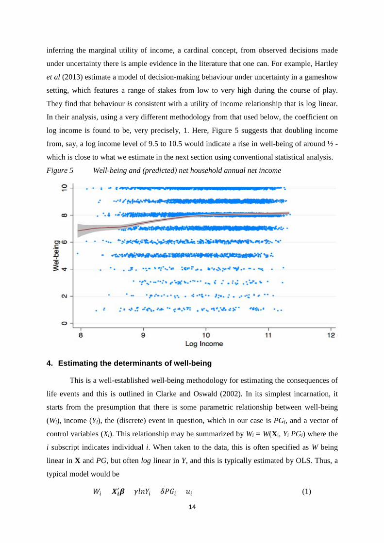
Figure 5 shows the scatterplot (with “jitter” applied to allow us to see how many

individuals are at each integer value in the graph from the density of the “blobs”) of predicted

net household income (by exponentiating the predicted log) against well-being, and

superimposes a local polynomial of the relationship between these two variables. This

relationship is relatively flat but does show a significant monotonically increasing

relationship that is concave over most of its range. If we think of this well-being vs income

relationship as a (expected) utility function then the concave nature would be consistent with

diminishing marginal utility of income. While there has been considerable controversy over

15 Another alternative is to use the midpoints of the income bins as the measure of income. Doing so makes no substantive difference to our findings – our money metric of lost wellbeing from problem gambling remains large and significant. However, since measurement error is not accounted for using this approach, the coefficient on household income simply becomes smaller, making our estimate of the cost of PG, even larger. 16 We exploit the detailed information on education included in BGPS, as well as age, age-squared, gender, self-assessed ethnicity, marital status, and an indicator of self-assessed health. Since our purpose in modelling income is to obtain a consistent prediction of the true level of income from the observed interval data we are not concerned with the exogeneity of the variables in this auxiliary equation. Variations in the precise specification of this interval regression make very little difference to our subsequent analysis.

14

inferring the marginal utility of income, a cardinal concept, from observed decisions made

under uncertainty there is ample evidence in the literature that one can. For example, Hartley

et al (2013) estimate a model of decision-making behaviour under uncertainty in a gameshow

setting, which features a range of stakes from low to very high during the course of play.

They find that behaviour is consistent with a utility of income relationship that is log linear.

In their analysis, using a very different methodology from that used below, the coefficient on

log income is found to be, very precisely, 1. Here, Figure 5 suggests that doubling income

from, say, a log income level of 9.5 to 10.5 would indicate a rise in well-being of around ½ -

which is close to what we estimate in the next section using conventional statistical analysis.

Figure 5 Well-being and (predicted) net household annual net income

4. Estimating the determinants of well-being

This is a well-established well-being methodology for estimating the consequences of

life events and this is outlined in Clarke and Oswald (2002). In its simplest incarnation, it

starts from the presumption that there is some parametric relationship between well-being

(Wi), income (Yi), the (discrete) event in question, which in our case is PGi, and a vector of

control variables (Xi). This relationship may be summarized by Wi = W(Xi, Yi PGi) where the

i subscript indicates individual i. When taken to the data, this is often specified as W being

linear in X and PG, but often log linear in Y, and this is typically estimated by OLS. Thus, a

typical model would be

𝑊𝑊𝑖𝑖 = 𝑿𝑿𝒊𝒊′𝜷𝜷 + 𝛾𝛾𝛾𝛾𝛾𝛾𝑌𝑌𝑖𝑖 + 𝛿𝛿𝑃𝑃𝑃𝑃𝑖𝑖 + 𝑢𝑢𝑖𝑖 (1)

15

where ui is the residual that captures variation in Wi that is not captured by the included

variables. Thus, the difference in well-being associated with PGi = 1 rather than 0 is simply

∆𝑊𝑊𝑖𝑖 = 𝛿𝛿. Since γ is the effect of a unit change in lnYi on well-being it follows that the same

difference in W could be achieved by changing lnYi by an amount equal to δ/γ. This implies

that δ/γ is the (percentage) change in Yi required to hold well-being at the level associated

with not being a problem gambler for i. This proportionate difference in Yi is often referred to

as the compensating variation (CV) – the percentage change in Yi required to compensate i

for being PGi=1.

The methodology is not, however, without its critics. The first criticism stems from

the fact that it is not at all clear that the scale of W from 1 to 10 can be given a cardinal

interpretation. That is, the restriction that moving from 1 to 2 is as good (bad) as a move from

4 to 5 is a strong one, impossible to verify, and hence difficult to rely on, in such data. It is

just as plausible that the move from 1 to 2, thereby doubling W, can only be achieved for

someone who has a W of 4 by moving to 8. It seems plausible that such a W measure could

well be monotonically increasing in true well-being, but that only the ordinal property can be

relied upon. To investigate the robustness of our conclusions on the impact of PG we, in

addition to estimating the conventional model where W is estimated by linear regression, also

provide estimates under the assumption that lnW is linear, and we further use a Box-Cox

estimation, which transforms the dependent variable in a way that nests both linear and log

linear and enables us to test against these special cases. In particular, we also estimate

𝑊𝑊𝑖𝑖𝜆𝜆−1

𝜆𝜆 = 𝑿𝑿𝒊𝒊′𝜷𝜷 + 𝛾𝛾𝛾𝛾𝛾𝛾𝑌𝑌𝑖𝑖 + 𝛿𝛿𝑃𝑃𝑃𝑃𝑖𝑖 + 𝑢𝑢𝑖𝑖, (2)

where λ=1 corresponds to the linear special case and λ=0 to the log case. We show below that

these alternative specifications make little difference to our PG money metric estimate.

A critical contribution to the well-being methodology by Bond and Lang (2010) raises

this ordinality issue. They note that since the W data is categorical, where the categories

represent intervals along some continuous distribution, the implied CDFs of these

distributions are likely to cross when estimated using large samples. Therefore, some

monotonic transformation of the utility function, W(.)¸ can always reverse the ranking of

overall well-being: for example, between the PG=1 group and the PG =0 group. Of course,

more categories will help resolve this problem, that would not arise if W were continuous, but

there is nothing to say that 10 categories is enough to ensure the reliability of the method. A

popular solution to this problem is to adopt a specification that only relies on the ordinal

16

nature of such well-being data. The simplest case is where one is prepared to assume that

well-being is Normally distributed so that we can easily fix the cut-points between 1, 2, 3 etc.

in which case we can estimate the means and variances of each group using Ordered Probit.

In particular, we estimate

𝑊𝑊𝑖𝑖∗ = 𝑿𝑿𝒊𝒊′𝜷𝜷 + 𝛾𝛾𝛾𝛾𝛾𝛾𝑌𝑌𝑖𝑖 + 𝛿𝛿𝑃𝑃𝑃𝑃𝑖𝑖 + 𝑢𝑢𝑖𝑖 (3)

where Wi = j if μj-1 < Wi* < μj, for j = 1,2,3,... 10, and ui is assumed to be Normal. Here μj are

the unknown cutpoints that are estimated by exploiting the assumed Normality of ui. In order

to compute the compensating variation in this ordered Probit case we need to transform the

coefficients into marginal effects, to make them comparable to the OLS coefficients, and then

cumulate the predicted probabilities across each of the levels of W, using the proportions

reporting each level of W as weights.

The second criticism of the method is a practical one – that, in practice, PG, is

measured with error. This will be true, not least, because PG is defined using self-reported

responses to the questions in the screen that is employed; and we notice that the different

screens produce different results (although insubstantially so). OLS estimates of δ, when PG

is subject to measurement error (ME), will be attenuated – i.e. biased towards zero (i.e.

downwards). The solution to a ME problem is to instrument with another measure (even one

that is also measured with error). When the ME is classical then IV produces consistent

estimates of δ. In practice, GMM estimation may be used to ensure consistency even if ME is

non-classical (see Kane et al, 1999, and Light and Flores-Lagunes, 2006). Fortunately, the

GPS data provides not just one screen for PG but two. Thus, we can instrument the PG

variable, computed from one screen according to whether the score exceeds the critical value,

with the score on the other screen. Indeed, the scores for each question within the alterative

screen might be used to form many instruments; although here we continue to adopt a

parsimonious approach and simply use the overall score from the alternate screen.

There remains one further criticism of this well-being methodology: one that is

generally ignored in the well-being literature generally, but was, nonetheless, a question that

was raised in Forrest (2104, 2016) in the present context of problem gambling. This criticism

is that PGi is itself endogenous - that is, it is correlated with both ui and Wi perhaps because

there are missing variables that confound the relationship. For example, in this context,

individuals with low Wi, for reasons that are not observed and controlled for, may be more

likely to have PGi=1. OLS estimation of δ will then be biased – upwards (downwards) if

17

cov(PGi,ui)>0 (<0) since δ will capture both the effect of PGi, and the effect of the

unobservables that are correlated with both PGi and Wi . We might expect that low well-being

types of people to be more likely to develop problem gambling (i.e. cov(PGi,ui) < 0) so OLS

estimates of the PG coefficient would be biased upwards. The solution to this problem is

again usually found through the use of instrumental variables. That is, we need to identify

some variable, call it Zi, that affects PGi but only affects Wi through its effect on PGi – that is,

there is no direct transmission between Zi and Wi.

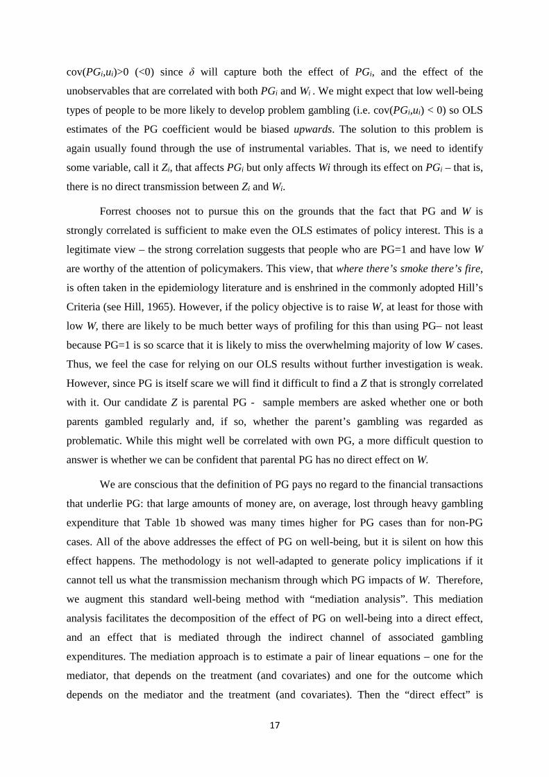
Forrest chooses not to pursue this on the grounds that the fact that PG and W is

strongly correlated is sufficient to make even the OLS estimates of policy interest. This is a

legitimate view – the strong correlation suggests that people who are PG=1 and have low W

are worthy of the attention of policymakers. This view, that where there’s smoke there’s fire,

is often taken in the epidemiology literature and is enshrined in the commonly adopted Hill’s

Criteria (see Hill, 1965). However, if the policy objective is to raise W, at least for those with

low W, there are likely to be much better ways of profiling for this than using PG– not least

because PG=1 is so scarce that it is likely to miss the overwhelming majority of low W cases.

Thus, we feel the case for relying on our OLS results without further investigation is weak.

However, since PG is itself scare we will find it difficult to find a Z that is strongly correlated

with it. Our candidate Z is parental PG - sample members are asked whether one or both

parents gambled regularly and, if so, whether the parent’s gambling was regarded as

problematic. While this might well be correlated with own PG, a more difficult question to

answer is whether we can be confident that parental PG has no direct effect on W.

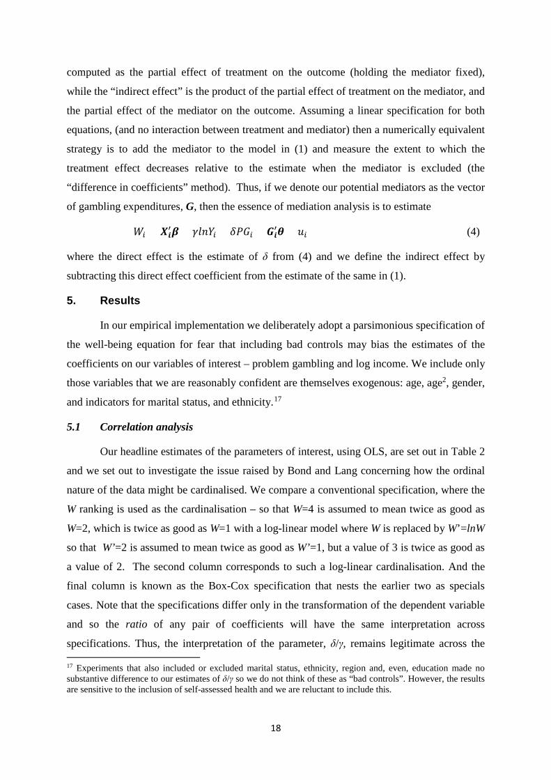
We are conscious that the definition of PG pays no regard to the financial transactions

that underlie PG: that large amounts of money are, on average, lost through heavy gambling

expenditure that Table 1b showed was many times higher for PG cases than for non-PG

cases. All of the above addresses the effect of PG on well-being, but it is silent on how this

effect happens. The methodology is not well-adapted to generate policy implications if it

cannot tell us what the transmission mechanism through which PG impacts of W. Therefore,

we augment this standard well-being method with “mediation analysis”. This mediation

analysis facilitates the decomposition of the effect of PG on well-being into a direct effect,

and an effect that is mediated through the indirect channel of associated gambling

expenditures. The mediation approach is to estimate a pair of linear equations – one for the

mediator, that depends on the treatment (and covariates) and one for the outcome which

depends on the mediator and the treatment (and covariates). Then the “direct effect” is

18

computed as the partial effect of treatment on the outcome (holding the mediator fixed),

while the “indirect effect” is the product of the partial effect of treatment on the mediator, and

the partial effect of the mediator on the outcome. Assuming a linear specification for both

equations, (and no interaction between treatment and mediator) then a numerically equivalent

strategy is to add the mediator to the model in (1) and measure the extent to which the

treatment effect decreases relative to the estimate when the mediator is excluded (the

“difference in coefficients” method). Thus, if we denote our potential mediators as the vector

of gambling expenditures, G, then the essence of mediation analysis is to estimate

𝑊𝑊𝑖𝑖 = 𝑿𝑿𝒊𝒊′𝜷𝜷 + 𝛾𝛾𝛾𝛾𝛾𝛾𝑌𝑌𝑖𝑖 + 𝛿𝛿𝑃𝑃𝑃𝑃𝑖𝑖 + 𝑮𝑮𝒊𝒊′𝜽𝜽 + 𝑢𝑢𝑖𝑖 (4)

where the direct effect is the estimate of δ from (4) and we define the indirect effect by

subtracting this direct effect coefficient from the estimate of the same in (1).

5. Results

In our empirical implementation we deliberately adopt a parsimonious specification of

the well-being equation for fear that including bad controls may bias the estimates of the

coefficients on our variables of interest – problem gambling and log income. We include only

those variables that we are reasonably confident are themselves exogenous: age, age2, gender,

and indicators for marital status, and ethnicity.17

5.1 Correlation analysis

Our headline estimates of the parameters of interest, using OLS, are set out in Table 2

and we set out to investigate the issue raised by Bond and Lang concerning how the ordinal

nature of the data might be cardinalised. We compare a conventional specification, where the

W ranking is used as the cardinalisation – so that W=4 is assumed to mean twice as good as

W=2, which is twice as good as W=1 with a log-linear model where W is replaced by W’=lnW

so that W’=2 is assumed to mean twice as good as W’=1, but a value of 3 is twice as good as

a value of 2. The second column corresponds to such a log-linear cardinalisation. And the

final column is known as the Box-Cox specification that nests the earlier two as specials

cases. Note that the specifications differ only in the transformation of the dependent variable

and so the ratio of any pair of coefficients will have the same interpretation across

specifications. Thus, the interpretation of the parameter, δ/γ, remains legitimate across the 17 Experiments that also included or excluded marital status, ethnicity, region and, even, education made no substantive difference to our estimates of δ/γ so we do not think of these as “bad controls”. However, the results are sensitive to the inclusion of self-assessed health and we are reluctant to include this.

19

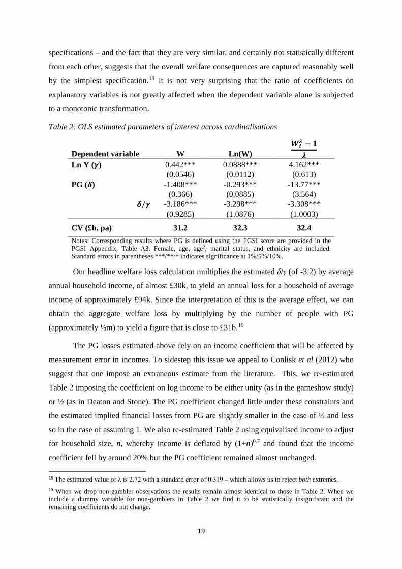
specifications – and the fact that they are very similar, and certainly not statistically different

from each other, suggests that the overall welfare consequences are captured reasonably well

by the simplest specification.18 It is not very surprising that the ratio of coefficients on

explanatory variables is not greatly affected when the dependent variable alone is subjected

to a monotonic transformation.

Table 2: OLS estimated parameters of interest across cardinalisations

Dependent variable W Ln(W) 𝑾𝑾𝒊𝒊

𝝀𝝀 − 𝟏𝟏𝝀𝝀

Ln Y (𝜸𝜸) 0.442*** 0.0888*** 4.162***

(0.0546) (0.0112) (0.613)

PG (𝜹𝜹) -1.408*** -0.293*** -13.77***

(0.366) (0.0885) (3.564)

𝜹𝜹/𝜸𝜸 -3.186*** -3.298*** -3.308*** (0.9285) (1.0876) (1.0003)

CV (£b, pa) 31.2 32.3 32.4 Notes: Corresponding results where PG is defined using the PGSI score are provided in the PGSI Appendix, Table A3. Female, age, age2, marital status, and ethnicity are included. Standard errors in parentheses ***/**/* indicates significance at 1%/5%/10%.

Our headline welfare loss calculation multiplies the estimated δ/γ (of -3.2) by average

annual household income, of almost £30k, to yield an annual loss for a household of average

income of approximately £94k. Since the interpretation of this is the average effect, we can

obtain the aggregate welfare loss by multiplying by the number of people with PG

(approximately ⅓m) to yield a figure that is close to £31b.19

The PG losses estimated above rely on an income coefficient that will be affected by

measurement error in incomes. To sidestep this issue we appeal to Conlisk et al (2012) who

suggest that one impose an extraneous estimate from the literature. This, we re-estimated

Table 2 imposing the coefficient on log income to be either unity (as in the gameshow study)

or ½ (as in Deaton and Stone). The PG coefficient changed little under these constraints and

the estimated implied financial losses from PG are slightly smaller in the case of ½ and less

so in the case of assuming 1. We also re-estimated Table 2 using equivalised income to adjust

for household size, n, whereby income is deflated by (1+n)0.7 and found that the income

coefficient fell by around 20% but the PG coefficient remained almost unchanged. 18 The estimated value of λ is 2.72 with a standard error of 0.319 – which allows us to reject both extremes. 19 When we drop non-gambler observations the results remain almost identical to those in Table 2. When we include a dummy variable for non-gamblers in Table 2 we find it to be statistically insignificant and the remaining coefficients do not change.

20

5.2 Causal analysis

However, these results are contingent on the exogeneity of PG which we relax in

Table 3. The first column corrects for measurement error in PG by exploiting the correlation

between the DSM definition of PG and the score from the alternative screen. The Staiger and

Stock (1997) rule of thumb that the first stage F statistic should exceed 10 is easily satisfied

for the results in the first column of Table 3, suggesting that the PGSI score is a very strong

instrument. The second column also includes parental PG in the instrument set in an attempt

to deal with the second potential source of endogeneity. The F statistic still satisfies the rule

of thumb. In each case, in Table 3, the PG coefficient is substantially larger than that in

Table 2. The crucial welfare effect, δ/γ, remains the same irrespective of the different

instruments used - with the exception of column 3 which uses Parental PG alone as an IV.

This does not produce as satisfactory an F in the first stage as the other cases - not

surprisingly the estimate of δ becomes much larger because the first stage only features ten

comliers, and it is common for the IV estimate to be even more biased than the OLS estimate

in such cases.

Table 3: Dependent variable, W: IV estimated parameters of interest.

Dependent variable Instruments

W PGSI score

W Parental PG and

PGSI score W

Parental PG

Ln Y (𝜸𝜸) 0.437*** 0.437*** 0.361***

(0.0526) (0.0570) (0.0841)

PG (𝜹𝜹) -2.512*** -2.527*** -20.115**

(0.6498) (0.6517) (9.5738)

𝜹𝜹/𝜸𝜸 -5.750*** -5.788*** -55.767* (1.6888) (1.6462) (34.5181)

CV (£b, pa) 56.3 56.7 546

First stage F 4904.66*** 1640.35*** 17.23*** Notes: Corresponding results where PG is defined using the PGSI score are provided in the PGSI Appendix, Table A3. Female, age, age2, marital status, and ethnicity are included as control variables. Estimated standard errors, obtained from bootsrapping, are in parentheses. ***/**/* indicates statistically significant at 1%/5%/10%. F is the Stock-Yogo definition – using the Windemeijer definition for multiple instruments in column 2 produces similar results.

21

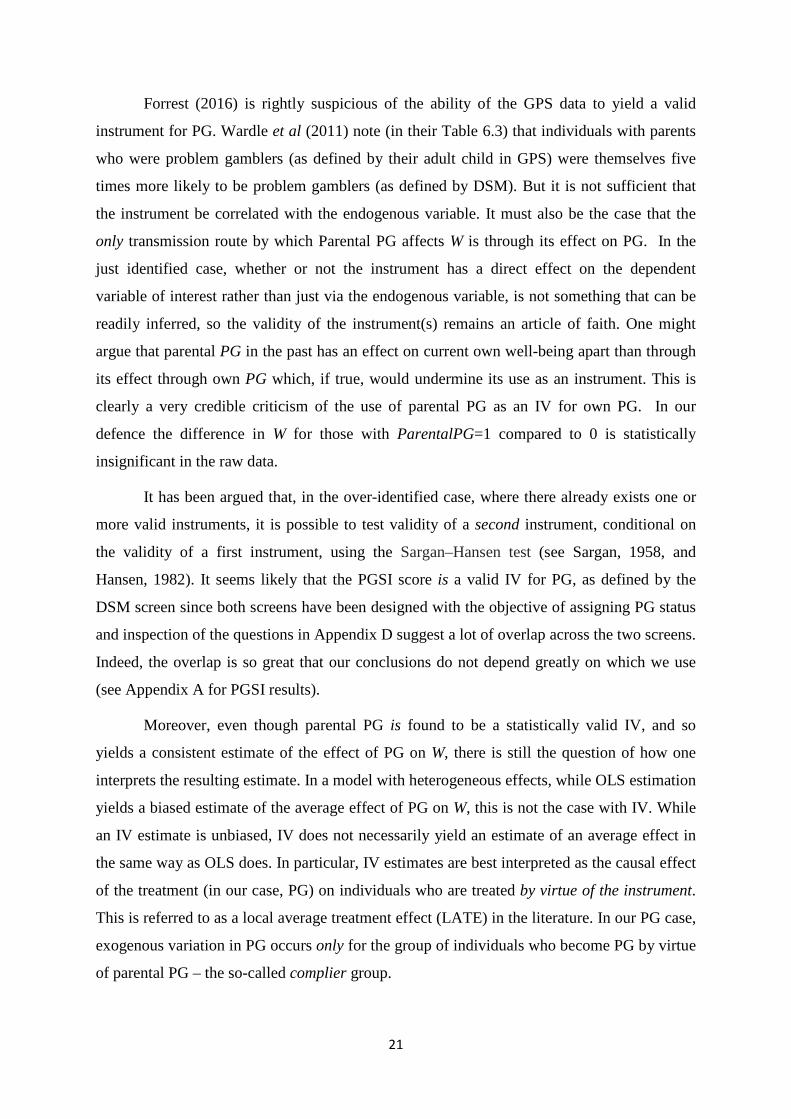
Forrest (2016) is rightly suspicious of the ability of the GPS data to yield a valid

instrument for PG. Wardle et al (2011) note (in their Table 6.3) that individuals with parents

who were problem gamblers (as defined by their adult child in GPS) were themselves five

times more likely to be problem gamblers (as defined by DSM). But it is not sufficient that

the instrument be correlated with the endogenous variable. It must also be the case that the

only transmission route by which Parental PG affects W is through its effect on PG. In the

just identified case, whether or not the instrument has a direct effect on the dependent

variable of interest rather than just via the endogenous variable, is not something that can be

readily inferred, so the validity of the instrument(s) remains an article of faith. One might

argue that parental PG in the past has an effect on current own well-being apart than through

its effect through own PG which, if true, would undermine its use as an instrument. This is

clearly a very credible criticism of the use of parental PG as an IV for own PG. In our

defence the difference in W for those with ParentalPG=1 compared to 0 is statistically

insignificant in the raw data.

It has been argued that, in the over-identified case, where there already exists one or

more valid instruments, it is possible to test validity of a second instrument, conditional on

the validity of a first instrument, using the Sargan–Hansen test (see Sargan, 1958, and

Hansen, 1982). It seems likely that the PGSI score is a valid IV for PG, as defined by the

DSM screen since both screens have been designed with the objective of assigning PG status

and inspection of the questions in Appendix D suggest a lot of overlap across the two screens.

Indeed, the overlap is so great that our conclusions do not depend greatly on which we use

(see Appendix A for PGSI results).

Moreover, even though parental PG is found to be a statistically valid IV, and so

yields a consistent estimate of the effect of PG on W, there is still the question of how one

interprets the resulting estimate. In a model with heterogeneous effects, while OLS estimation

yields a biased estimate of the average effect of PG on W, this is not the case with IV. While

an IV estimate is unbiased, IV does not necessarily yield an estimate of an average effect in

the same way as OLS does. In particular, IV estimates are best interpreted as the causal effect

of the treatment (in our case, PG) on individuals who are treated by virtue of the instrument.

This is referred to as a local average treatment effect (LATE) in the literature. In our PG case,

exogenous variation in PG occurs only for the group of individuals who become PG by virtue

of parental PG – the so-called complier group.

22

Some applied econometricians have argued that, while we do not necessarily obtain

an estimate of the average effect of the treatment in question on a readily identifiable

population we nonetheless estimate something that is still relevant for policy. In contrast

others argue that a LATE estimate is not useful and we need to augment it with something

else to produce economically meaningful parameters (e.g. a structural econometric model). In

our case, unlike the case of a schooling reform instrument used in Harmon and Walker (1995)

in search of the causal effect of education on wages, it is difficult to argue that the adults

were so affected by parental PG that they became PG themselves, especially because this

group is so small. In particular, it is quite conceivable that Parental PG makes some people

more likely to be PG (compliers) through some common environment or even genes. But is

also possible that there are defiers – people who observe their parents were PG and were

determined not to become like that. Formally, IV LATE estimates are the weighted average

of the defier and complier estimates. Ideally we would like to pursue a matching

methodology to attempt to support the IV estimates. However, since the PG group is so very

small it is not likely that we would ever be able to get good matches. Similarly, one might

like to pursue the bounding idea in Altonji, Elder and Taber (2006). However, again the

treatment group is so small the bounds will inevitably be huge.

In the specification using both PGSI score and parental problem gambling as

instruments we test the validity of our instruments using Hansen’s J-test for over-

identification and this fails to reject the null hypothesis that our first-stage instruments are

valid. However, the Hansen test (and earlier Sargan test) are not generally applicable in the

context of a model where there are heterogeneous effects. Fortunately, we do not have to rely

on this test because Table 3 suggests that nothing much hangs on the case for using Parental

PG as an IV – we get the same results when we drop Parental PG and use the alternative

PGSI score as the only instrument. The welfare relevant parameter, δ/γ, is virtually the same

in both columns. The suggestion is that it is measurement error in PG that accounts for much

of the bias in the OLS estimate in column 1 of Table 2. This is fortunate since it implies that

we can extrapolate from our IV estimates. Thus, if we take δ/γ to be -5.75 then this implies an

average welfare effect of around £170k pppa which we can then aggregate to approximately

£56b pa.20

20 We find that dropping non-gamblers, or including a dummy variable for non-gamblers, makes no difference to the results in Table 3.

23

We also re-estimated Table 3 including exactly the same set of exogenous variables in

both first and second stages. The second stage results of the relevant parameters were almost

identical to the ones provided above. We also explored the sensitivity of our results, in

column 1 of Table 2, to how income is defined. We have two choices in the BGPS data –

individual net income, or household net income. The tables here use (log) household level

income. Replacing this by (predicted log) individual level income (again from an interval

regression), we find a slightly smaller income effect. However, household income is

approximately double the level of individual level and so the corresponding welfare loss

measures, using the household definition, are somewhat larger than we found with individual

income.21 For example, using predicted log individual income the aggregate CV for the basic

OLS specification is £21b rather than £31b. If we use the (log of) the midpoint of the bin

which each individual reports (whether at individual or at household level) yield much

smaller estimates than when use the predicted log from the interval regression. This is to be

expected and the large difference is indicative of considerable measurement error in the raw

binned data as well as the inappropriateness of using the midpoint when the raw income data

is highly left skewed. So we strongly prefer the estimates reported in this section.

A further issue, is the appropriateness of the definition of PG itself. The DSM (and

PGSI) score comes from simply adding up the responses to each question, so attributing them

with equal weight in terms of their effect on well-being. A simple alternative would be to

allow the data to decide by including controls for each of the 10 (9) questions. Doing this we

find that only one of the 10 DSM questions has a statistically significant effect on W: Q5

which, not surprisingly, asks “Have you gambled to escape from problems …” and we find

that a test of the joint insignificance of the remaining questions fails to reject. If we then

dropped the insignificant questions, so that PG is defined simply by Q5, and instrument that

with the PGSI score (without also including Parental PG) then we get a coefficient of -0.85

(0.26), or (with including Parental PG) -0.88 (0.26) – larger (if only slightly so) than Table 3

suggests.

21 A minor problem with household income is that there is a coding mistake in the raw data that cannot be fixed – two different income bins shared the same code on the income showcard. One solution to this problem is to recode the observations that chose either of these two codes as missing. Two alternatives would be to check by adding up the (midpoint of the binned) individual level data and replace accordingly; or, similarly, use STATAs missing values routine to construct a replacement exploiting the relationship between household and individual incomes in the data. None of these methods made any effective difference to our estimates.

24

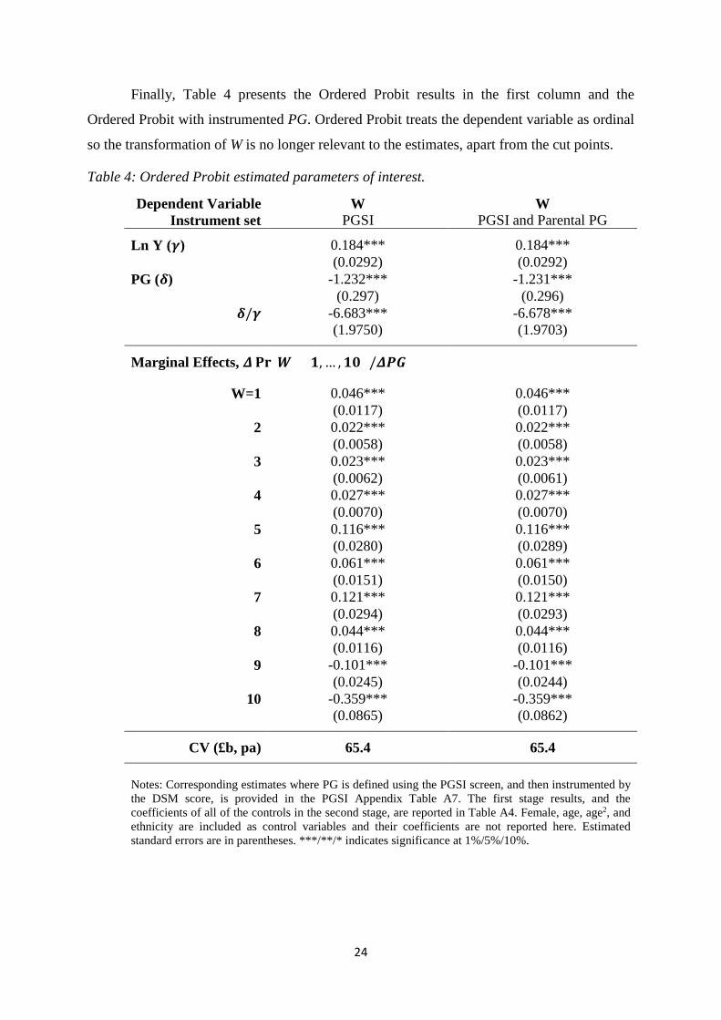
Finally, Table 4 presents the Ordered Probit results in the first column and the

Ordered Probit with instrumented PG. Ordered Probit treats the dependent variable as ordinal

so the transformation of W is no longer relevant to the estimates, apart from the cut points.

Table 4: Ordered Probit estimated parameters of interest.

Dependent Variable Instrument set

W PGSI

W PGSI and Parental PG

Ln Y (𝜸𝜸) 0.184*** 0.184***

(0.0292) (0.0292)

PG (𝜹𝜹) -1.232*** -1.231***

(0.297) (0.296)

𝜹𝜹/𝜸𝜸 -6.683*** -6.678***

(1.9750) (1.9703)

Marginal Effects, 𝜟𝜟𝐏𝐏𝐏𝐏(𝑾𝑾 = 𝟏𝟏, … ,𝟏𝟏𝟏𝟏) /𝜟𝜟𝜟𝜟𝑮𝑮

W=1 0.046*** 0.046***

(0.0117) (0.0117)

2 0.022*** 0.022***

(0.0058) (0.0058)

3 0.023*** 0.023***

(0.0062) (0.0061)

4 0.027*** 0.027***

(0.0070) (0.0070)

5 0.116*** 0.116***

(0.0280) (0.0289)

6 0.061*** 0.061***

(0.0151) (0.0150)

7 0.121*** 0.121***

(0.0294) (0.0293)

8 0.044*** 0.044***

(0.0116) (0.0116)

9 -0.101*** -0.101***

(0.0245) (0.0244)

10 -0.359*** -0.359***

(0.0865) (0.0862)

CV (£b, pa) 65.4 65.4 Notes: Corresponding estimates where PG is defined using the PGSI screen, and then instrumented by the DSM score, is provided in the PGSI Appendix Table A7. The first stage results, and the coefficients of all of the controls in the second stage, are reported in Table A4. Female, age, age2, and ethnicity are included as control variables and their coefficients are not reported here. Estimated standard errors are in parentheses. ***/**/* indicates significance at 1%/5%/10%.

25

However, interpretation is more difficult in the context of Ordered Probit since the

marginal effects of LnY and PG rely on these parameters, and on the cut point estimates

which are not reported. For any cardinalisation of W, we would expect PG to lower the

probability of high W and increase the probability of low W. Using Ordered Probit to estimate

the annual cost of lost welfare to afflicted individuals is slightly more involved than in the

OLS (or other) cases. Similar to the OLS and IV cases, we take the ratio of estimated

marginal effects of ln(Y) and PG on W and multiply by the proportion of afflicted individuals,

mean income and population size. However, these must be calculated using the marginal

effects and mean income for each value of W to correctly estimate the cost.

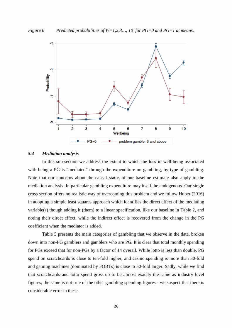
The marginal effects reported in the bottom half of Table 4 describe the effects of PG

on the probability that W=1, 2…..,10. There are positive significant effects of PG=1 (as

opposed to 0) on the probability of having low W, and negative effects on the probability that

W is high. Figure 6 plots the probability of W = 1, 2, 3…,10 at the averages of the other

explanatory variables, for the PG = 1 and 0 groups, using the estimates from the bottom half

of column 2 of Table 4. The figure also shows the confidence intervals around these predicted

probabilities of being at each level of W by PG. The PG = 0 group is much larger so the

confidence intervals are much tighter. Nonetheless, the estimates separate the groups very

well. There are statistically significantly larger probabilities of PG = 1 individuals having

values of W below 7 compared to PG = 0 individuals; and significantly larger probabilities of

PG = 0 individuals having values of W above 7 compared to PG=1 individuals22. The cost

estimates provided in Table 4, of £65b, are the summation of this calculation for W=1,…,10,

weighted by the proportion of our sample who report each well-being level.

22 Extending the IV analysis to the ordered Probit case is not straightforward. Chesher and Smolinski (2012) show that control function methods in this case impose unrealistic restrictions, and are set, rather than point, identified. However, they show that this problem becomes less severe the less discrete the dependent variable is.

26

Figure 6 Predicted probabilities of W=1,2,3…, 10 for PG=0 and PG=1 at means.

5.4 Mediation analysis

In this sub-section we address the extent to which the loss in well-being associated

with being a PG is “mediated” through the expenditure on gambling, by type of gambling.

Note that our concerns about the causal status of our baseline estimate also apply to the

mediation analysis. In particular gambling expenditure may itself, be endogenous. Our single

cross section offers no realistic way of overcoming this problem and we follow Huber (2016)

in adopting a simple least squares approach which identifies the direct effect of the mediating

variable(s) though adding it (them) to a linear specification, like our baseline in Table 2, and

noting their direct effect, while the indirect effect is recovered from the change in the PG

coefficient when the mediator is added.

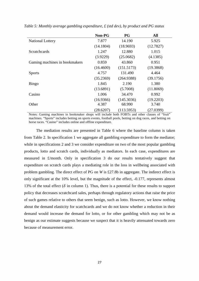
Table 5 presents the main categories of gambling that we observe in the data, broken

down into non-PG gamblers and gamblers who are PG. It is clear that total monthly spending

for PGs exceed that for non-PGs by a factor of 14 overall. While lotto is less than double, PG

spend on scratchcards is close to ten-fold higher, and casino spending is more than 30-fold

and gaming machines (dominated by FOBTs) is close to 50-fold larger. Sadly, while we find

that scratchcards and lotto spend gross-up to be almost exactly the same as industry level

figures, the same is not true of the other gambling spending figures - we suspect that there is

considerable error in these.

27

Table 5: Monthly average gambling expenditure, £ (std dev), by product and PG status

Non-PG PG All

National Lottery 7.877 14.190 5.925

(14.1804) (18.9693) (12.7827)

Scratchcards 1.247 12.880 1.015

(3.9229) (25.0682) (4.1385)

Gaming machines in bookmakers 0.859 43.860 0.951

(16.4600) (151.5173) (19.3868)

Sports 4.757 131.490 4.464

(35.2369) (264.9388) (39.1756)

Bingo 1.845 2.190 1.380

(13.6891) (5.7008) (11.8069)

Casino 1.006 34.470 0.992

(16.9366) (145.3036) (19.2203)

Other 4.387 68.990 3.740

(28.6207) (113.5953) (27.0399)

Notes: Gaming machines in bookmaker shops will include both FOBTs and other classes of “fruit” machines. “Sports” includes betting on sports events, football pools, betting on dog races, and betting on horse races. “Casino” includes online and offline expenditure.

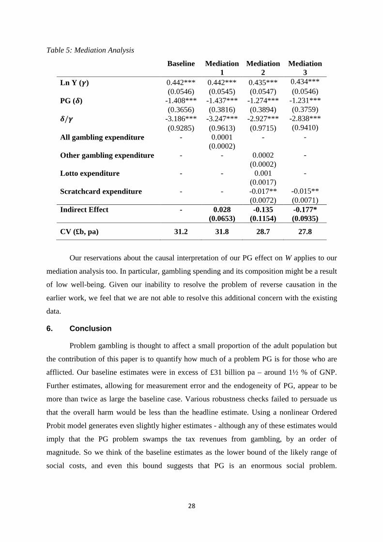
The mediation results are presented in Table 6 where the baseline column is taken

from Table 2. In specification 1 we aggregate all gambling expenditure to form the mediator;

while in specifications 2 and 3 we consider expenditure on two of the most popular gambling

products, lotto and scratch cards, individually as mediators. In each case, expenditures are

measured in £/month. Only in specification 3 do our results tentatively suggest that

expenditure on scratch cards plays a mediating role in the loss in wellbeing associated with

problem gambling. The direct effect of PG on W is £27.8b in aggregate. The indirect effect is

only significant at the 10% level, but the magnitude of the effect, -0.177, represents almost

13% of the total effect (𝛿𝛿 in column 1). Thus, there is a potential for these results to support

policy that decreases scratchcard sales, perhaps through regulatory actions that raise the price

of such games relative to others that seem benign, such as lotto. However, we know nothing

about the demand elasticity for scatchcards and we do not know whether a reduction in their

demand would increase the demand for lotto, or for other gambling which may not be as

benign as our estimate suggests because we suspect that it is heavily attenuated towards zero

because of measurement error.

28

Table 5: Mediation Analysis

Baseline

Mediation 1

Mediation 2

Mediation 3

Ln Y (𝜸𝜸) 0.442*** 0.442*** 0.435*** 0.434***

(0.0546) (0.0545) (0.0547) (0.0546)

PG (𝜹𝜹) -1.408*** -1.437*** -1.274*** -1.231***

(0.3656) (0.3816) (0.3894) (0.3759)

𝜹𝜹/𝜸𝜸 -3.186*** -3.247*** -2.927*** -2.838*** (0.9285) (0.9613) (0.9715) (0.9410) All gambling expenditure - 0.0001 - - (0.0002) Other gambling expenditure - - 0.0002 - (0.0002) Lotto expenditure - - 0.001 - (0.0017) Scratchcard expenditure - - -0.017** -0.015** (0.0072) (0.0071) Indirect Effect -

0.028

(0.0653) -0.135

(0.1154) -0.177* (0.0935)

CV (£b, pa) 31.2 31.8 28.7 27.8

Our reservations about the causal interpretation of our PG effect on W applies to our

mediation analysis too. In particular, gambling spending and its composition might be a result

of low well-being. Given our inability to resolve the problem of reverse causation in the

earlier work, we feel that we are not able to resolve this additional concern with the existing

data.

6. Conclusion

Problem gambling is thought to affect a small proportion of the adult population but

the contribution of this paper is to quantify how much of a problem PG is for those who are

afflicted. Our baseline estimates were in excess of £31 billion pa – around 1½ % of GNP.

Further estimates, allowing for measurement error and the endogeneity of PG, appear to be

more than twice as large the baseline case. Various robustness checks failed to persuade us

that the overall harm would be less than the headline estimate. Using a nonlinear Ordered

Probit model generates even slightly higher estimates - although any of these estimates would

imply that the PG problem swamps the tax revenues from gambling, by an order of

magnitude. So we think of the baseline estimates as the lower bound of the likely range of

social costs, and even this bound suggests that PG is an enormous social problem.

29

Unfortunately, we are not able to provide any direct comparisons with the previous literature

or with alternative methodologies.23

Given the potential size of this problem it would be important to design the policy

response to it by exploring the transmission mechanism by which PG develops. Only if the

transmission of PG was mediated via gambling expenditure may it then make sense to use

gambling tax policy to reduce the extent of transmission. Even if this were the case this

would not necessarily imply that gambling should be made illegal, or even taxed more

heavily. There is the additional consideration of the consumer surplus enjoyed by players -

the overwhelming majority of which appear to experience little or no problem with this

activity. If we interpret our estimates of the loss in well-being associated with PG in the spirit

of Orphanides and Zervos (1995), then our average estimate already incorporates the positive

well-being enjoyed by those who are lucky enough to gamble without regret. If one were not

prepared to accept this interpretation then the cross section work in Farrell and Walker (2000)

and the time series work reported in Walker and Wheeler (2016) provide estimates of the

price elasticity of demand for lotto that would imply that the consumer surplus enjoyed by

lotto players is in the order of £1 billion pa. If we could extrapolate from this to the rest of

gambling spending, then the aggregate consumer surplus across all forms of gambling would

still be very small in comparison with the welfare losses reported here24.

Nonetheless, taxing gambling more highly would only be part of the solution to the

PG problem if gambling expenditure was an important mediator for PG. The lottery draw and

scratchcard spending in the GPS data does suggest a correlation with PG: PG=1 individuals

spend around twice as much on lottery draw games as do PG=0, and around 10 times as

much on scratchcards25. In addition, as Forrest (2014) points out, we would need to be able

23 However Forrest (2016), while not addressing the range of econometric issues that are of concern here, supports our conclusion that the PG problem is a very serious one by showing that his estimates of PG on well-being for men was of a similar order of magnitude as that of being a widower, relative to being married. Indeed, for women, he found that, the effect of PG on W was even larger than that of being a widow on W. 24 However, the take-out for non-lottery forms of gambling are subject to take out rates that would typically be less than 10% so we might be underestimating the consumer surplus enjoyed through these other sources of gambling. 25 BGPS contains data on monthly spending, reported in intervals, for every type of gambling for those that say they engage in each type. The lottery draw spending grosses up, using the bin mid-points, to £3.20b, almost exactly matching the official annual sales (of £3.16b), but the scratchcard spending underestimates official sales (of £1.34b) by approximately 14%. Respondents are allowed to say that they would prefer not to say how much they spend and this is not an insubstantial proportion of those that report buying scratchcards in the last year. It is likely that these refusniks are larger than average spenders and we do not capture this in our calculations which are therefore best thought of as a lower bound. There are clear differences in the gambling spending of

30

to argue that the elasticity of gambling demand was high, especially for those with PG26. The

absence of evidence that taxation would reduce expenditure and that expenditure matters

causally for PG is an important priority for future work. In any event, given the highly

skewed nature of PG, there may be a case for trying to profile problem gamblers and apply

treatments that do not rely on financial incentives solely to those that have a high probability

of PG, rather than imposing some policy intervention onto the population as a whole,

especially when doing so would harm the overwhelming majority of non-PG cases. Sadly,

our reduced-form work shows that there are very few variables that are significantly

indicative of PG.

Our exploratory mediation results suggest that scratchcards may play a mediating role

in the impact of PG on well-being, while other products do not, which suggests a role for

policy that generates substitution effects towards more benign products. However,

measurement error implies that we can say nothing about the role of other forms of gambling.

PG=1 and PG=0 individuals. PG=1 spend £308 per month and lotto is 5% of this. While PG=0 spend £16 per month and lotto accounts for around 35% of this. Investigating the extent to which expenditure, and its composition, is an important part of the transmission mechanism that determines PG is a topic for future research. 26 Intuitively, we would expect addicted consumers to be exhibit less elastic demand. So taxation might have little effect on the behaviour of addicts but nonetheless cause a large deadweight loss on those who are not addicted. While estimates of the average elasticity for various types of gambling do exist (see the report by Frontier Economics, 2014), there appear to none that allow for heterogeneity across the distribution of gambling. See Hollingsworth et al (2016) for the case of alcohol demand.

31

References

Angrist, J.D. and J-S. Pischke (2009), Mostly Harmless Econometrics: An Empiricist's Companion, Princeton University Press.

Altonji, J.G., T.E. Elder and C.R. Taber (2005), “Selection on Observed and Unobserved Variables:”, Journal of Political Economy, 113, 51-184.

Australian Productivity Commission (2010), Gambling, Australian Productivity Commission Inquiry Report 50, Commonwealth of Australia.

Becker, G.S. (1964), Human Capital: A Theoretical and Empirical Analysis, with Special Reference to Education, Columbia University Press for NBER, New York.

Becker, G.S. and K. M. Murphy (1988), “A Theory of Rational Addiction”, Journal of Political Economy, 96, 675-700.

Becker, G.S., M. Grossman, and K. M. Murhpy, (2006), “The Market for Illegal Goods: The Case of Drugs”, Journal of Political Economy, 114, 38-60.

Black, D.A., M.C. Berger, and F.A. Scott, 2000, “Bounding Parameter Estimates with Nonclassical Measurement Error”, Journal of the American Statistical Association, 95, 739-748.

Bond, T.A. and K. Lang (2010), “The sad truth about happiness scales”, NBER WP19950.

Chesher, A. and K. Smolinski (2012), “IV models of ordered choice”, Journal of Econometrics, 166, 33-48.

Clarke, A. and A. Oswald (2002), “A simple statistical method for measuring how life events affect happiness”, International Journal of Epidemiology, 31, 1139-1144.

Conley, T.G., C.B. Hansen, and P.E. Rossi (2012), Plausibly Exogeneous, Review of Economics and Statistics, 94, 260–272

Deaton, A. and A.A. Stone (2013), “Two happiness puzzles”, American Economic Review (Papers and Proceedings), 103, 591–597.

Delfabbro, D. (2010), A Review of Australian Gambling Research: Implications for Inter-Jurisdictional Public Policy and Regulation: Update Report, http://www.gamblingresearch.org.au/home/research/gra+research+reports/a+review+of+australian+gambling+research+2010 .

Downs, C. (2014), “Gambling on Debt: Problem Gamblers Strategies for Concealing Deviant Identities”, Presentation to the AGRI Conference, Alberta, 2014. http://dspace.ucalgary.ca/bitstream/1880/49991/7/Downs_AGRI_Conference_2014.pdf

Farrell, L. and I. Walker (1999), “The Welfare Effects of Lotto”, Journal of Public Economics, 72, 99-120

Forrest, D. (2014), “An Economic and Social Review of Gambling in Great Britain”, Journal of Gambling Business and Economics, 7, 1-33.

Forrest, D. (2016), “The Unhappiness of Problem Gamblers”, mimeo.

Frontier Economics (2014), “The UK betting and gaming market: estimating price elasticities of demand and understanding the use of promotions”, Report to HMRC.

32

Griffiths, M. (2014), “Problem gambling in Great Britain: A brief review”, Report for the Association of British Bookmakers. Available at http://abb.uk.com/wp-content/uploads/2014/09/Problem-Gambling-in-Great-Britain-A-Brief-Review.pdf.

Gruber, J. and B. Koszegi, (2001), “Is Addiction "Rational"? Theory and Evidence,” Quarterly Journal of Economics, 116,1261-1303.

Hansen, L.P. (1982), “Large Sample Properties of Generalized Method of Moments Estimators”, Econometrica, 50, 1029–1054.

Harmon, C. and I. Walker (1995), “Estimates of the Economic Return to Schooling: Evidence from the UK”, American Economic Review, 85, 1278-1286.

Hill, A.B. (1965). “The Environment and Disease: Association or Causation?”, Proceedings of the Royal Society of Medicine. 58, 295–300.

Hollingsworth, B., R. Pryce, and I. Walker (2016), “The Differing Response to Alcohol Price Changes: Quantity and Quality”, mimeo.

Huber, M. (2016), “Disentangling policy effects into causal channels”, IZA World of Labor, doi: 10.15185/izawol.259.

Institutes of Advanced Studies (2013), “Economic Impacts of Alcohol - Factsheet”, http://www.ias.org.uk/uploads/pdf/Factsheets/Economic%20impacts%20of%20alcohol%20factsheet%20August%202013.pdf

Kane, T.J., Rouse, C., and Staiger, D (1999), “Estimating returns to schooling when schooling is misreported”, National Bureau of Economic Research WP 7235.

Layard, R. (2005), Happiness: Lessons from a New Science, London, Penguin.

Light, A. and A. Flores-Lagunes (2006), “Measurement error in schooling: Evidence from siblings and identical twins”, B.E. Journal of Economic Analysis and Policy, 5, 1.

Mincer, J.A. (1974), “The Human Capital Earnings Function”, in J.A. Mincer (ed.) Schooling, Experience, and Earnings, NBER.

Nikolova, M. (2106), “Happiness and Development”, IZA Discussion Paper 10088.

Orford, J., K. Sproston, B. Evans, C. White, and L. Mitchell (2003), Gambling and Problem Gambling in Britain, Brunner-Routledge.

Orford, J., H. Wardle, and M. Griffiths (2013), “What proportion of gambling is problem gambling? Estimates from the 2010 British Gambling Prevalence Survey”, International Gambling Studies, 13, 4-18.

Orphanides, A. and D. Zervos (1995), “Rational Addiction with Learning and Regret”, Journal of Political Economy, 103, 739-758.

Powdthavee, N. (2010), "How much does money really matter? Estimating the causal effects of income on happiness", Empirical Economics, 39, 77-92.

Powdthavee, N. and B. van den Berg (2011), “Putting different price tags on the same health condition: Re-evaluating the well-being valuation approach”, Journal of Health Economics, 30, 1032–1043.

Sargan, J. D. (1958), “The Estimation of Economic Relationships Using Instrumental Variables”, Econometrica, 26, 393–415.

Shaffer and D.A. Korn (2002), “Gambling and related mental disorders: a public health analysis”, Annual Review of Public Health, 23, 171–212

33

Staiger, D., and J. H. Stock (1997): “Instrumental Variables Regression with Weak Instruments,” Econometrica, 65, 557–86.

Stock, J. H., J. H. Wright, and M. Yogo (2002), “A Survey of Weak Instruments and Weak Identification in Generalized Method of Moments,” Journal of Business and Economic Statistics, 20, 518–29.

Sussman, S., N. Lisha, and M. Griffiths (2011), "Prevalence of the addictions: a problem of the majority or the minority?" Evaluation and the Health Professions. 34, 3-56.

Thorley C., A. Stirling, and E. Huynh (2016), Cards on the table - The cost to government associated with people who are problem gamblers in Britain, IPPR Report.

Walker, I. and R. Wheeler (2016), “The Economics of Lotto Design”, mimeo.

Wardle, H., A. Moody, S. Spence, J. Orford, D. Jotangia, R. Volberg, D. M. Griffiths, D. Hussey, and F. Dobbie (2011), British Gambling Prevalence Survey 2010. London: The Stationery Office.

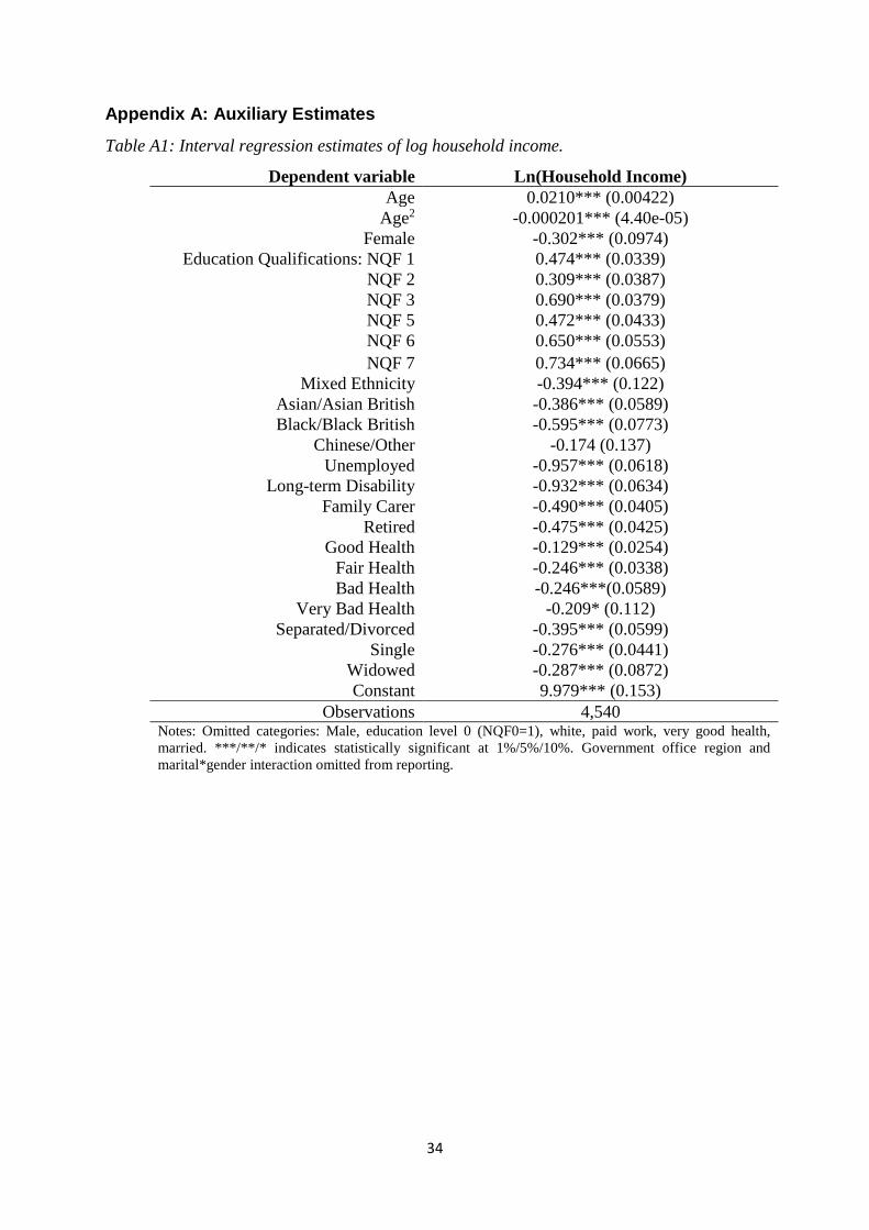
34

Appendix A: Auxiliary Estimates

Table A1: Interval regression estimates of log household income.

Dependent variable Ln(Household Income) Age 0.0210*** (0.00422)

Age2 -0.000201*** (4.40e-05) Female -0.302*** (0.0974)

Education Qualifications: NQF 1 0.474*** (0.0339) NQF 2 0.309*** (0.0387) NQF 3 0.690*** (0.0379) NQF 5 0.472*** (0.0433) NQF 6 0.650*** (0.0553) NQF 7 0.734*** (0.0665)

Mixed Ethnicity -0.394*** (0.122) Asian/Asian British -0.386*** (0.0589) Black/Black British -0.595*** (0.0773)

Chinese/Other -0.174 (0.137) Unemployed -0.957*** (0.0618)

Long-term Disability -0.932*** (0.0634) Family Carer -0.490*** (0.0405)

Retired -0.475*** (0.0425) Good Health -0.129*** (0.0254)

Fair Health -0.246*** (0.0338) Bad Health -0.246***(0.0589)

Very Bad Health -0.209* (0.112) Separated/Divorced -0.395*** (0.0599)

Single -0.276*** (0.0441) Widowed -0.287*** (0.0872) Constant 9.979*** (0.153)

Observations 4,540 Notes: Omitted categories: Male, education level 0 (NQF0=1), white, paid work, very good health, married. ***/**/* indicates statistically significant at 1%/5%/10%. Government office region and marital*gender interaction omitted from reporting.

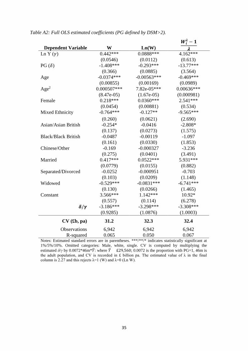
35

Table A2: Full OLS estimated coefficients (PG defined by DSM>2).

Dependent Variable W Ln(W) 𝑾𝑾𝒊𝒊

𝝀𝝀 − 𝟏𝟏𝝀𝝀

Ln Y (𝛾𝛾) 0.442*** 0.0888*** 4.162***

(0.0546) (0.0112) (0.613)

PG (𝛿𝛿) -1.408*** -0.293*** -13.77***

(0.366) (0.0885) (3.564)

Age -0.0374*** -0.00563*** -0.469***

(0.00855) (0.00169) (0.0989)

Age2 0.000507*** 7.82e-05*** 0.00636***

(8.47e-05) (1.67e-05) (0.000981)

Female 0.218*** 0.0360*** 2.541***

(0.0454) (0.00881) (0.534)

Mixed Ethnicity -0.764*** -0.127** -9.565***

(0.260) (0.0621) (2.690)

Asian/Asian British -0.254* -0.0416 -2.808*

(0.137) (0.0273) (1.575)

Black/Black British -0.0487 -0.00119 -1.097

(0.161) (0.0330) (1.853)

Chinese/Other -0.169 -0.000327 -3.236

(0.275) (0.0401) (3.491)

Married 0.417*** 0.0522*** 5.931***

(0.0779) (0.0155) (0.882)

Separated/Divorced -0.0252 -0.000951 -0.703

(0.103) (0.0209) (1.148)

Widowed -0.529*** -0.0831*** -6.741***

(0.130) (0.0266) (1.465)

Constant 3.566*** 1.142*** 10.92*

(0.557) (0.114) (6.278)

𝜹𝜹/𝜸𝜸 -3.186*** -3.298*** -3.308*** (0.9285) (1.0876) (1.0003)

CV (£b, pa) 31.2 32.3 32.4 Observations 6,942 6,942 6,942

R-squared 0.065 0.050 0.067 Notes: Estimated standard errors are in parentheses. ***/**/* indicates statistically significant at 1%/5%/10%. Omitted categories: Male, white, single. CV is computed by multiplying the estimated δ/γ by 0.0072*46m*𝑌𝑌�: where 𝑌𝑌� = £29,560; 0.0072 is the proportion with PG=1, 46m is the adult population, and CV is recorded in £ billion pa. The estimated value of λ in the final column is 2.27 and this rejects λ=1 (W) and λ=0 (Ln W).

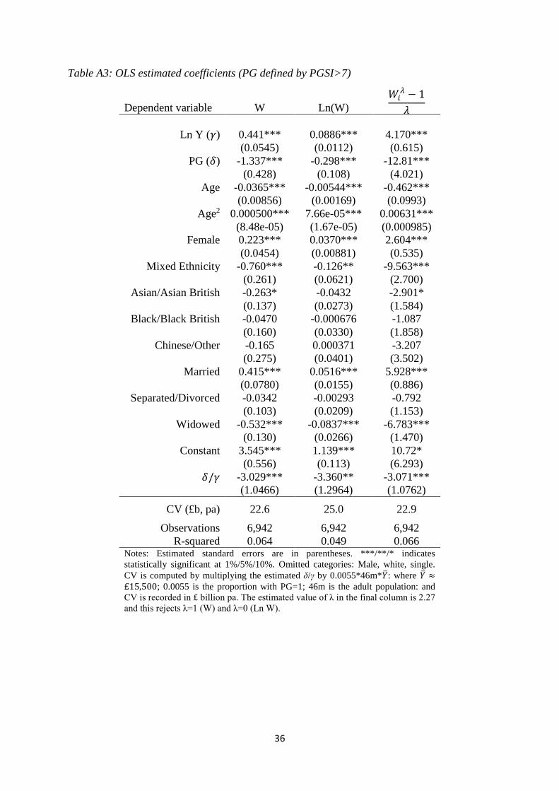
36

Table A3: OLS estimated coefficients (PG defined by PGSI>7)

Dependent variable W Ln(W) 𝑊𝑊𝑖𝑖

𝜆𝜆 − 1𝜆𝜆

Ln Y (𝛾𝛾) 0.441*** 0.0886*** 4.170***

(0.0545) (0.0112) (0.615)

PG (𝛿𝛿) -1.337*** -0.298*** -12.81***

(0.428) (0.108) (4.021)

Age -0.0365*** -0.00544*** -0.462***

(0.00856) (0.00169) (0.0993)

Age2 0.000500*** 7.66e-05*** 0.00631***

(8.48e-05) (1.67e-05) (0.000985)

Female 0.223*** 0.0370*** 2.604***

(0.0454) (0.00881) (0.535)

Mixed Ethnicity -0.760*** -0.126** -9.563***

(0.261) (0.0621) (2.700)

Asian/Asian British -0.263* -0.0432 -2.901*

(0.137) (0.0273) (1.584)

Black/Black British -0.0470 -0.000676 -1.087

(0.160) (0.0330) (1.858)

Chinese/Other -0.165 0.000371 -3.207

(0.275) (0.0401) (3.502)

Married 0.415*** 0.0516*** 5.928***

(0.0780) (0.0155) (0.886)

Separated/Divorced -0.0342 -0.00293 -0.792

(0.103) (0.0209) (1.153)

Widowed -0.532*** -0.0837*** -6.783***

(0.130) (0.0266) (1.470)

Constant 3.545*** 1.139*** 10.72*

(0.556) (0.113) (6.293)

𝛿𝛿/𝛾𝛾 -3.029*** -3.360** -3.071*** (1.0466) (1.2964) (1.0762)

CV (£b, pa) 22.6 25.0 22.9

Observations 6,942 6,942 6,942 R-squared 0.064 0.049 0.066

Notes: Estimated standard errors are in parentheses. ***/**/* indicates statistically significant at 1%/5%/10%. Omitted categories: Male, white, single. CV is computed by multiplying the estimated δ/γ by 0.0055*46m*𝑌𝑌�: where 𝑌𝑌� ≈£15,500; 0.0055 is the proportion with PG=1; 46m is the adult population: and CV is recorded in £ billion pa. The estimated value of λ in the final column is 2.27 and this rejects λ=1 (W) and λ=0 (Ln W).

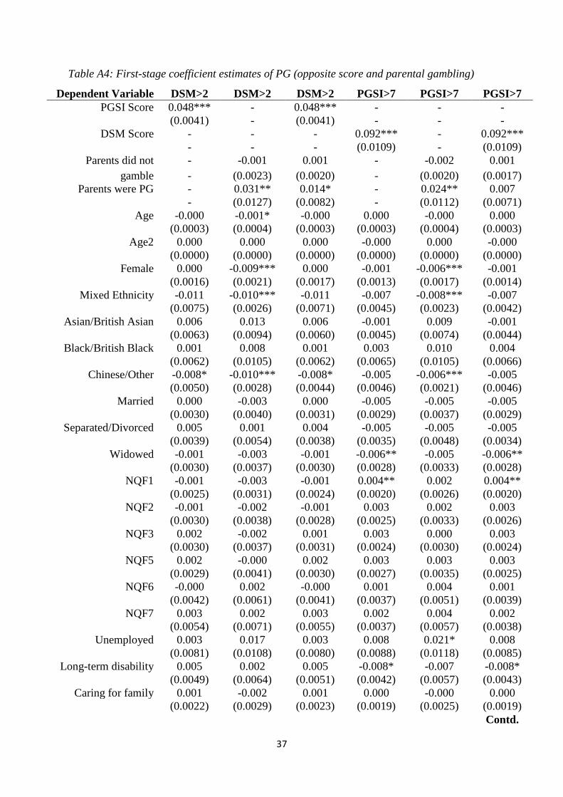
37

Table A4: First-stage coefficient estimates of PG (opposite score and parental gambling)

Dependent Variable DSM>2 DSM>2 DSM>2 PGSI>7 PGSI>7 PGSI>7 PGSI Score 0.048*** - 0.048*** - - -

(0.0041) - (0.0041) - - -

DSM Score - - - 0.092*** - 0.092***

- - - (0.0109) - (0.0109)

Parents did not - -0.001 0.001 - -0.002 0.001 gamble - (0.0023) (0.0020) - (0.0020) (0.0017)

Parents were PG - 0.031** 0.014* - 0.024** 0.007

- (0.0127) (0.0082) - (0.0112) (0.0071)

Age -0.000 -0.001* -0.000 0.000 -0.000 0.000

(0.0003) (0.0004) (0.0003) (0.0003) (0.0004) (0.0003)

Age2 0.000 0.000 0.000 -0.000 0.000 -0.000

(0.0000) (0.0000) (0.0000) (0.0000) (0.0000) (0.0000)

Female 0.000 -0.009*** 0.000 -0.001 -0.006*** -0.001

(0.0016) (0.0021) (0.0017) (0.0013) (0.0017) (0.0014)

Mixed Ethnicity -0.011 -0.010*** -0.011 -0.007 -0.008*** -0.007

(0.0075) (0.0026) (0.0071) (0.0045) (0.0023) (0.0042)

Asian/British Asian 0.006 0.013 0.006 -0.001 0.009 -0.001

(0.0063) (0.0094) (0.0060) (0.0045) (0.0074) (0.0044)

Black/British Black 0.001 0.008 0.001 0.003 0.010 0.004

(0.0062) (0.0105) (0.0062) (0.0065) (0.0105) (0.0066)

Chinese/Other -0.008* -0.010*** -0.008* -0.005 -0.006*** -0.005

(0.0050) (0.0028) (0.0044) (0.0046) (0.0021) (0.0046)

Married 0.000 -0.003 0.000 -0.005 -0.005 -0.005

(0.0030) (0.0040) (0.0031) (0.0029) (0.0037) (0.0029)

Separated/Divorced 0.005 0.001 0.004 -0.005 -0.005 -0.005

(0.0039) (0.0054) (0.0038) (0.0035) (0.0048) (0.0034)

Widowed -0.001 -0.003 -0.001 -0.006** -0.005 -0.006**

(0.0030) (0.0037) (0.0030) (0.0028) (0.0033) (0.0028)

NQF1 -0.001 -0.003 -0.001 0.004** 0.002 0.004**

(0.0025) (0.0031) (0.0024) (0.0020) (0.0026) (0.0020)

NQF2 -0.001 -0.002 -0.001 0.003 0.002 0.003

(0.0030) (0.0038) (0.0028) (0.0025) (0.0033) (0.0026)

NQF3 0.002 -0.002 0.001 0.003 0.000 0.003

(0.0030) (0.0037) (0.0031) (0.0024) (0.0030) (0.0024)

NQF5 0.002 -0.000 0.002 0.003 0.003 0.003

(0.0029) (0.0041) (0.0030) (0.0027) (0.0035) (0.0025)

NQF6 -0.000 0.002 -0.000 0.001 0.004 0.001

(0.0042) (0.0061) (0.0041) (0.0037) (0.0051) (0.0039)

NQF7 0.003 0.002 0.003 0.002 0.004 0.002

(0.0054) (0.0071) (0.0055) (0.0037) (0.0057) (0.0038)

Unemployed 0.003 0.017 0.003 0.008 0.021* 0.008

(0.0081) (0.0108) (0.0080) (0.0088) (0.0118) (0.0085)

Long-term disability 0.005 0.002 0.005 -0.008* -0.007 -0.008* (0.0049) (0.0064) (0.0051) (0.0042) (0.0057) (0.0043)

Caring for family 0.001 -0.002 0.001 0.000 -0.000 0.000 (0.0022) (0.0029) (0.0023) (0.0019) (0.0025) (0.0019) Contd.

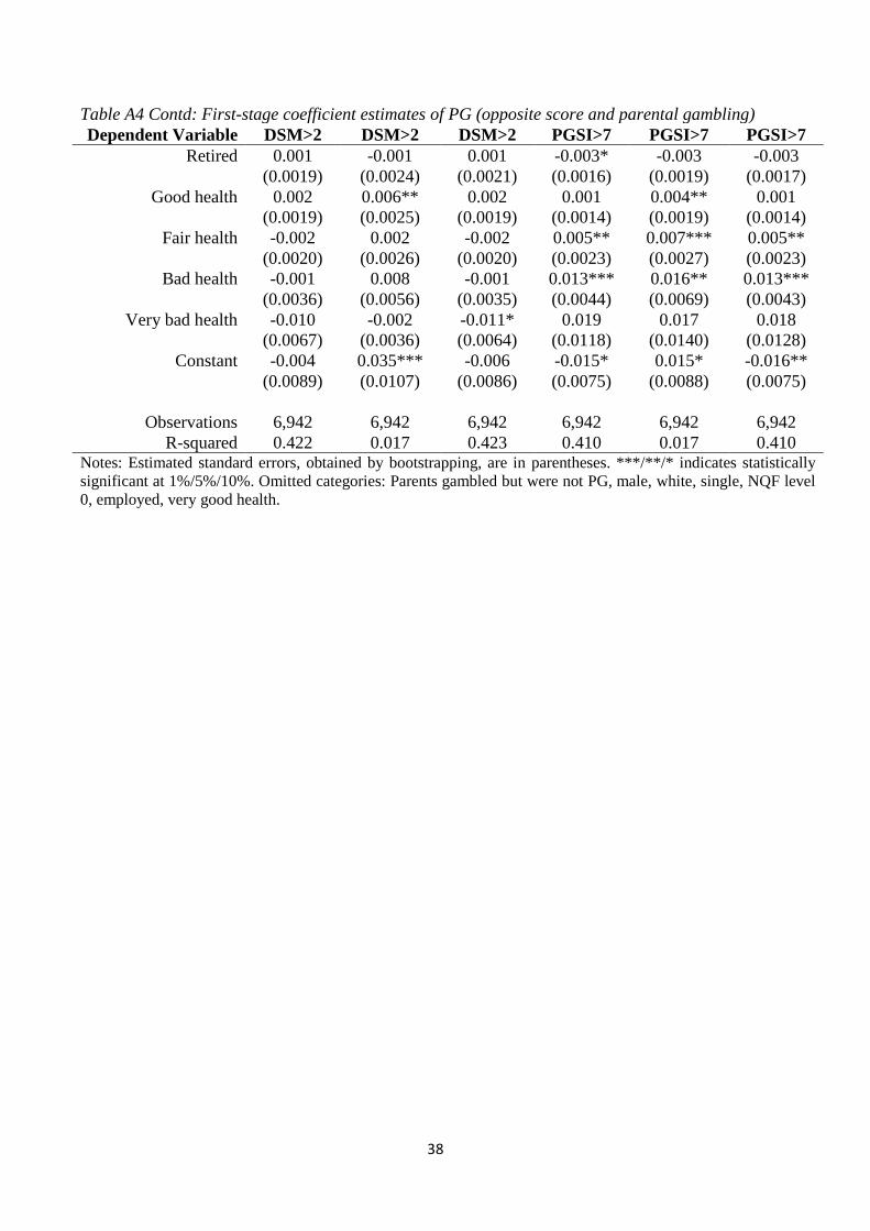
38

Table A4 Contd: First-stage coefficient estimates of PG (opposite score and parental gambling) Dependent Variable DSM>2 DSM>2 DSM>2 PGSI>7 PGSI>7 PGSI>7

Retired 0.001 -0.001 0.001 -0.003* -0.003 -0.003

(0.0019) (0.0024) (0.0021) (0.0016) (0.0019) (0.0017)

Good health 0.002 0.006** 0.002 0.001 0.004** 0.001

(0.0019) (0.0025) (0.0019) (0.0014) (0.0019) (0.0014)

Fair health -0.002 0.002 -0.002 0.005** 0.007*** 0.005**

(0.0020) (0.0026) (0.0020) (0.0023) (0.0027) (0.0023)

Bad health -0.001 0.008 -0.001 0.013*** 0.016** 0.013***

(0.0036) (0.0056) (0.0035) (0.0044) (0.0069) (0.0043)

Very bad health -0.010 -0.002 -0.011* 0.019 0.017 0.018

(0.0067) (0.0036) (0.0064) (0.0118) (0.0140) (0.0128)

Constant -0.004 0.035*** -0.006 -0.015* 0.015* -0.016**

(0.0089) (0.0107) (0.0086) (0.0075) (0.0088) (0.0075)

Observations 6,942 6,942 6,942 6,942 6,942 6,942 R-squared 0.422 0.017 0.423 0.410 0.017 0.410

Notes: Estimated standard errors, obtained by bootstrapping, are in parentheses. ***/**/* indicates statistically significant at 1%/5%/10%. Omitted categories: Parents gambled but were not PG, male, white, single, NQF level 0, employed, very good health.

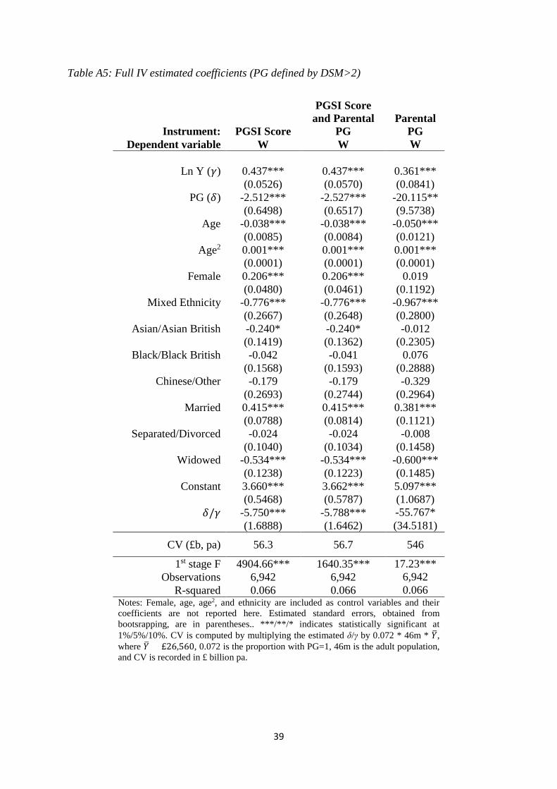
39

Table A5: Full IV estimated coefficients (PG defined by DSM>2)

Instrument: PGSI Score

PGSI Score and Parental

PG

Parental PG

Dependent variable W W W

Ln Y (𝛾𝛾) 0.437*** 0.437*** 0.361***

(0.0526) (0.0570) (0.0841)

PG (𝛿𝛿) -2.512*** -2.527*** -20.115**

(0.6498) (0.6517) (9.5738)

Age -0.038*** -0.038*** -0.050***

(0.0085) (0.0084) (0.0121)

Age2 0.001*** 0.001*** 0.001***

(0.0001) (0.0001) (0.0001)

Female 0.206*** 0.206*** 0.019

(0.0480) (0.0461) (0.1192)

Mixed Ethnicity -0.776*** -0.776*** -0.967***

(0.2667) (0.2648) (0.2800)

Asian/Asian British -0.240* -0.240* -0.012

(0.1419) (0.1362) (0.2305)

Black/Black British -0.042 -0.041 0.076

(0.1568) (0.1593) (0.2888)

Chinese/Other -0.179 -0.179 -0.329

(0.2693) (0.2744) (0.2964)

Married 0.415*** 0.415*** 0.381***

(0.0788) (0.0814) (0.1121)

Separated/Divorced -0.024 -0.024 -0.008

(0.1040) (0.1034) (0.1458)

Widowed -0.534*** -0.534*** -0.600***

(0.1238) (0.1223) (0.1485)

Constant 3.660*** 3.662*** 5.097***

(0.5468) (0.5787) (1.0687)

𝛿𝛿/𝛾𝛾 -5.750*** -5.788*** -55.767* (1.6888) (1.6462) (34.5181)

CV (£b, pa) 56.3 56.7 546

1st stage F 4904.66*** 1640.35*** 17.23*** Observations 6,942 6,942 6,942

R-squared 0.066 0.066 0.066 Notes: Female, age, age2, and ethnicity are included as control variables and their coefficients are not reported here. Estimated standard errors, obtained from bootsrapping, are in parentheses.. ***/**/* indicates statistically significant at 1%/5%/10%. CV is computed by multiplying the estimated δ/γ by 0.072 * 46m * 𝑌𝑌�, where 𝑌𝑌� = £26,560, 0.072 is the proportion with PG=1, 46m is the adult population, and CV is recorded in £ billion pa.

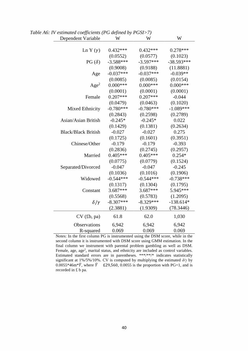
40

Table A6: IV estimated coefficients (PG defined by PGSI>7) Dependent Variable W W W

Ln Y (𝛾𝛾) 0.432*** 0.432*** 0.278***

(0.0552) (0.0577) (0.1023)

PG (𝛿𝛿) -3.588*** -3.597*** -38.593***

(0.9008) (0.9188) (11.8881)

Age -0.037*** -0.037*** -0.039**

(0.0085) (0.0085) (0.0154)

Age2 0.000*** 0.000*** 0.000***

(0.0001) (0.0001) (0.0001)

Female 0.207*** 0.207*** -0.044

(0.0479) (0.0463) (0.1020)

Mixed Ethnicity -0.780*** -0.780*** -1.089***

(0.2843) (0.2598) (0.2789)

Asian/Asian British -0.245* -0.245* 0.022

(0.1429) (0.1381) (0.2634)

Black/Black British -0.027 -0.027 0.275

(0.1725) (0.1601) (0.3951)

Chinese/Other -0.179 -0.179 -0.393

(0.2836) (0.2745) (0.2957)

Married 0.405*** 0.405*** 0.254*

(0.0775) (0.0779) (0.1524)

Separated/Divorced -0.047 -0.047 -0.245

(0.1036) (0.1016) (0.1906)

Widowed -0.544*** -0.544*** -0.738***

(0.1317) (0.1304) (0.1795)

Constant 3.687*** 3.687*** 5.945***

(0.5568) (0.5783) (1.2095)

𝛿𝛿/𝛾𝛾 -8.307*** -8.329*** -138.614* (2.3881) (1.9309) (78.3446)

CV (£b, pa) 61.8 62.0 1,030

Observations 6,942 6,942 6,942 R-squared 0.069 0.069 0.069

Notes: In the first column PG is instrumented using the DSM score, while in the second column it is instrumented with DSM score using GMM estimation. In the final column we instrument with parental problem gambling as well as DSM. Female, age, age2, marital status, and ethnicity are included as control variables. Estimated standard errors are in parentheses. ***/**/* indicates statistically significant at 1%/5%/10%. CV is computed by multiplying the estimated δ/γ by 0.0055*46m*𝑌𝑌�, where 𝑌𝑌� = £29,560, 0.0055 is the proportion with PG=1, and is recorded in £ b pa.

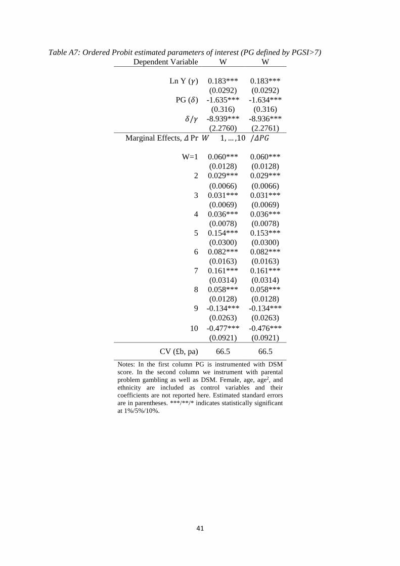
41

Table A7: Ordered Probit estimated parameters of interest (PG defined by PGSI>7) Dependent Variable W W

Ln Y (𝛾𝛾) 0.183*** 0.183***

(0.0292) (0.0292)

PG (𝛿𝛿) -1.635*** -1.634***

(0.316) (0.316)

𝛿𝛿/𝛾𝛾 -8.939*** -8.936***

(2.2760) (2.2761)

Marginal Effects, 𝛥𝛥 Pr(𝑊𝑊 = 1, … ,10) /𝛥𝛥𝑃𝑃𝑃𝑃)

W=1 0.060*** 0.060***

(0.0128) (0.0128)

2 0.029*** 0.029***

(0.0066) (0.0066)

3 0.031*** 0.031***

(0.0069) (0.0069)

4 0.036*** 0.036***

(0.0078) (0.0078)

5 0.154*** 0.153***

(0.0300) (0.0300)

6 0.082*** 0.082***

(0.0163) (0.0163)

7 0.161*** 0.161***

(0.0314) (0.0314)

8 0.058*** 0.058***

(0.0128) (0.0128)

9 -0.134*** -0.134***

(0.0263) (0.0263)

10 -0.477*** -0.476***

(0.0921) (0.0921)

CV (£b, pa) 66.5 66.5 Notes: In the first column PG is instrumented with DSM score. In the second column we instrument with parental problem gambling as well as DSM. Female, age, age2, and ethnicity are included as control variables and their coefficients are not reported here. Estimated standard errors are in parentheses. ***/**/* indicates statistically significant at 1%/5%/10%.

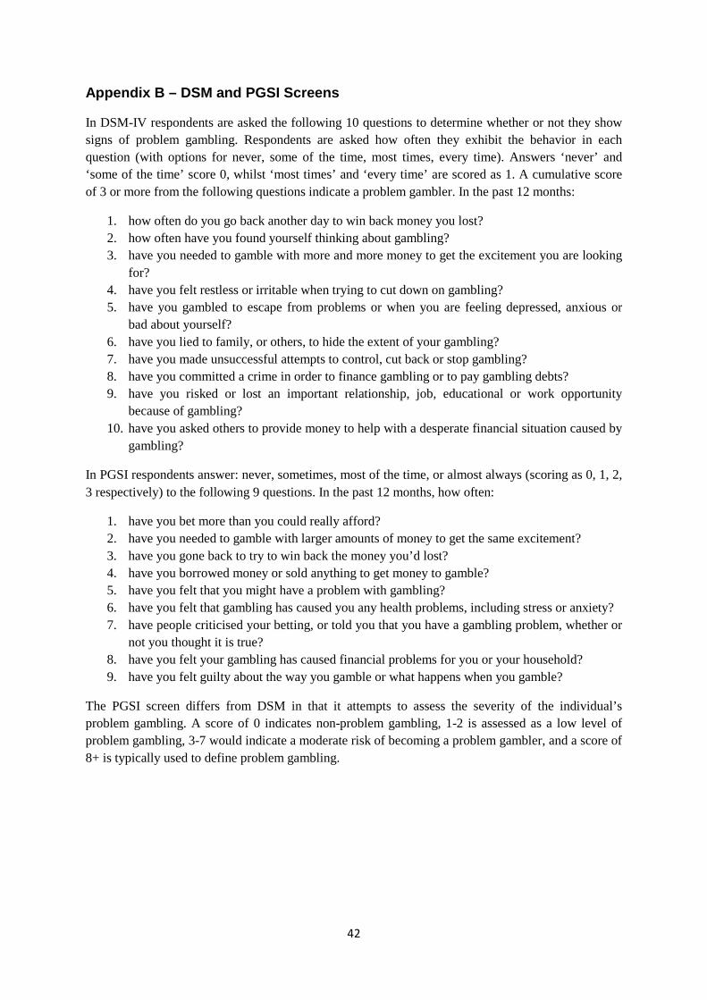
42

Appendix B – DSM and PGSI Screens

In DSM-IV respondents are asked the following 10 questions to determine whether or not they show signs of problem gambling. Respondents are asked how often they exhibit the behavior in each question (with options for never, some of the time, most times, every time). Answers ‘never’ and ‘some of the time’ score 0, whilst ‘most times’ and ‘every time’ are scored as 1. A cumulative score of 3 or more from the following questions indicate a problem gambler. In the past 12 months:

1. how often do you go back another day to win back money you lost? 2. how often have you found yourself thinking about gambling? 3. have you needed to gamble with more and more money to get the excitement you are looking

for? 4. have you felt restless or irritable when trying to cut down on gambling? 5. have you gambled to escape from problems or when you are feeling depressed, anxious or

bad about yourself? 6. have you lied to family, or others, to hide the extent of your gambling? 7. have you made unsuccessful attempts to control, cut back or stop gambling? 8. have you committed a crime in order to finance gambling or to pay gambling debts? 9. have you risked or lost an important relationship, job, educational or work opportunity

because of gambling? 10. have you asked others to provide money to help with a desperate financial situation caused by

gambling?

In PGSI respondents answer: never, sometimes, most of the time, or almost always (scoring as 0, 1, 2, 3 respectively) to the following 9 questions. In the past 12 months, how often:

1. have you bet more than you could really afford? 2. have you needed to gamble with larger amounts of money to get the same excitement? 3. have you gone back to try to win back the money you’d lost? 4. have you borrowed money or sold anything to get money to gamble? 5. have you felt that you might have a problem with gambling? 6. have you felt that gambling has caused you any health problems, including stress or anxiety? 7. have people criticised your betting, or told you that you have a gambling problem, whether or

not you thought it is true? 8. have you felt your gambling has caused financial problems for you or your household? 9. have you felt guilty about the way you gamble or what happens when you gamble?

The PGSI screen differs from DSM in that it attempts to assess the severity of the individual’s problem gambling. A score of 0 indicates non-problem gambling, 1-2 is assessed as a low level of problem gambling, 3-7 would indicate a moderate risk of becoming a problem gambler, and a score of 8+ is typically used to define problem gambling.