economics output shocks in china: do the … · economics . output shocks in china: do the...
TRANSCRIPT
ECONOMICS
OUTPUT SHOCKS IN CHINA: DO THE DISTRIBUTIONAL EFFECTS DEPEND ON THE
REGIONAL SOURCE?
by
Anping Chen
School of Economics Jinan University, China
and
Nicolaas Groenewold Business School
University of Western Australia
DISCUSSION PAPER 16.20
OUTPUT SHOCKS IN CHINA: DO THE DISTRIBUTIONAL EFFECTS DEPEND ON THE REGIONAL SOURCE?
Anping Chen
School of Economics, Jinan University,
Guangzhou, China ([email protected])
and
Nicolaas Groenewold
Economics Programme, UWA Business School, M251,
University of Western Australia, Perth, Australia
DISCUSSION PAPER 16.20 ABSTRACT The tension between growth and inequality in the process of economic development has been recognised in the research literature as well as in policy-making circles for many decades. In few countries in the modern world is this problem more acute than in China where inter-provincial disparities are large by world standards and where remarkable economic growth in the past three decades has tended sooner to widen than to narrow them. Not surprisingly, the source of such inter-provincial disparities in China has been the subject of considerable research. Yet we have relatively little empirical knowledge of the effects on the provincial distribution of output of shocks to macroeconomic variables such as GDP. This is an important gap in the empirical literature: macroeconomic shocks are likely to have a differential impact on the provincial economies and so affect the provincial output distribution. Policy-makers need to know the sign, size and timing of such effects before making policy decisions designed to influence output at the national or regional level. In this paper we focus on the regional source of national shocks and ask whether the effect at the provincial level depends on the regional source of the shock. We use two alternative methods for this. The first is one recently employed by Chen and Groenewold (2015) to analyse the provincial effects of shocks to national output and investment using a restricted VAR model due to Lastrapes (2005). The method extends their work by disaggregating national GDP into three regional outputs – for the coastal, central and western regions of China. Our second method uses a sequence of VAR models, each with three regional outputs and one provincial output. We find that the two methods give remarkably similar results – both provide strong evidence that a shock to a particular region’s output has its main effects on the provinces in that region, although this is more marked in the short run than in the long run and differs somewhat across regions. In particular, a shock to national output which originates in the coastal region has an affect mainly on the coastal provinces in both the short and long runs. Such a shock is therefore likely to exacerbate existing inter-provincial disparities. However, there is more diffusion of the effects of a central shock, particularly in the long run which may help alleviate disparities. A shock to the western region also generates spillover effects in the long run although these are to the coastal provinces and will therefore likely widen existing disparities. (415 words) Keywords: provincial output distribution, regional shocks, regional disparities, economic growth, China JEL categories: E61, R50, O53 *Corresponding author. Acknowledgements. An earlier version of this paper was presented at the Workshop on Regional, Urban and Spatial Economics at South-West University of Finance and Economics in Chengdu and at the Meeting of the European Regional Science Association in Vienna. We are grateful for useful comments received there. The research reported in this paper was partially funded by a National Natural Science Foundation of China Grant (No. 71173092) and the Program for New Century Excellent Talents in University, Ministry of Education of China (No. NCET-12-0681).
1
1. Introduction
It has long been recognised that, in the process of economic development, there may
well be a trade-off between growth and inequality. Those familiar with the literature on
economic development and on regional development in particular, will realise that the
consideration of such a trade-off is not new. Indeed, it dates back at least to the work on the
inverted-U curve between economic development and inequality associated in particular with
Williamson (1965) and earlier work by Kuznets (1955), Myrdal (1957) and Hirschman
(1958). The idea captured by the inverted-U curve is that in the early stages of development
regional (and other) inequality rises but eventually falls as development gathers pace. There
is thus a systematic relationship between inequality and development which has an inverted-
U shape.
Not only does the issue of growth versus equality have a long history, but it is an area
of active current research as evidenced by a special issue of Spatial Economic Analysis (see
the introductory essay by Lopez-Bazo et al., 2014) and a survey paper by Cunha Neves and
Tavares Silva (2014). Both papers reflect the thrust of earlier literature that the issue is far
from settled and the relationship between growth and inequality depends not only on the
precise measures used and the sample periods and countries examined, but also on the drivers
of growth. Moreover, the causal direction between the two variables is not clear a priori,
with the sign of the relationship between them potentially depending on the direction of
causation (see, e.g., Chen, 2010 and Kraay, 2015).
In few countries in the developing world has the problem of the trade-off between
growth and inequality been more acute than in China. Although China has grown at
remarkably high and sustained rates since opening-up and reforms began to take hold in the
1980s, there have been substantial and persistent problems with the distribution of this
expanding output. A commonly used measure of dispersion, the coefficient of variation, fell
2
steadily over two decades from the late 1970s until the late 1990s after which it began to rise
so that by 2004 it had returned to the level of the mid-1980s; it then declined.1 A paper by
Lemoine et al. (2014) confirms the observed recent decline in inequality and relates it to the
growing convergence in manufacturing although another paper, Lyhagen and Rickne (2014),
reports mixed evidence, with roughly half the possible province-pairs showing convergence
and the remainder divergence.2 Whatever the precise nature of recent change in inequality,
inter-provincial disparities remain a serious problem with the ratio of real GDP per capita in
the richest province in 2014 (Jiangsu) to that of the poorest (Guizhou) still at 3.1, a very large
disparity by any standards.3
Since the inception of the People’s Republic of China, the uneven regional
distribution of output has been a perennial policy issue at the highest levels of Chinese
policy-making as well as in academic policy discussions.4 Yet, there has been a noticeable
caution in the vigour with which such policies are pursued by policy makers who are
reluctant to jeopardise the continuation of a high aggregate growth rate. There has also been
a noticeable ambiguity in the policy/empirical literature on whether growth can be achieved
at the same time as addressing regional inequality. Thus, Kuijs and Wang (2005) argues
1 This characterisation is based on the coefficient of variation for nominal provincial GDP per capita from 1978 to 2014. While there may be some evidence of the narrowing of inter-provincial income differentials, it seems that the inter-personal income distribution is becoming more unequal; a recent IMF Discussion Paper argues that “Income inequality—as measured by the Gini coefficient for pre-tax market income—has exhibited an increasing trend from 0.28 in 1980 to 0.44 in 2000 and 0.52 by 2013. There is also significant within-China variation in income inequality at the regional level. This widening in the gap between rich and poor shows China’s transition from a relatively egalitarian society to one of the most unequal countries in the world.” (Cevik and Correa-Caro, 2015, p. 3). 2 The question of exactly whether, and, if so, how and when regional economies in China have been converging has been the subject of a great deal of empirical research. To survey this would take us too far afield in this introduction but see Groenewold et al. (2008) Chapter 2 and the interesting contribution by Andersson et al. (2013) and references there. 3 This comparison excludes the “city-provinces” of Shanghai, Beijing and Tianjin for which the comparable ratios are even higher at 3.7, 3.8 and 4.0 respectively in 2014. 4 See Groenewold et al. (2008), Chapter 3, Xu et al. (2013) and Chen (2013) for more information on Chinese regional policy since the founding of the People’s Republic of China. See Zhao and Tong (2000) for an earlier call for the reconsideration of the “coastal development strategy” because of its implications for regional disparities and Groenewold et al. (2010) for a more recent discussion. Knight (2016) provides an interesting general discussion of the possible conflict between economic growth and other objectives, including equality.
3
growth and inequality reduction are not inconsistent for China while Wong (2006), Knight
(2008), Zhu and Wan (2012) and Li et al. (2016) express the opposite view.
Although there has been much discussion of the possibility for China to pursue both
growth and equality, there has been only limited empirical analysis of this question. Some
papers touch on the issue indirectly. Thus, Qiao et al. (2008) analyses it in the context of the
effects of fiscal decentralisation while Wu and Yao (2015) examines the importance of the
presence of SOEs in the economy for the growth-inequality relationship and Zheng and
Kuroda (2013) considers the drivers of growth and their importance for the growth-inequality
relationship.
Wan et al. (2006) directly tests the growth-inequality nexus in China, focusing on
rural-urban income inequality and regional growth using a provincial-level panel data set.
They find that reductions in inequality will be growth-enhancing. A different direct approach
has been taken in Chen (2010) which reports tests of the relationship between growth in per
capita GDP and a specific measure of inequality (the Gini coefficient) in a multivariate time-
series model. It is found that a reduction in inequality comes at the cost of growth in the
short run but not in the long run. A similar analysis is reported in Risso and Sanchez Carrera
(2012) and an extension to three variables (with saving being the additional variable) is
reported in Gu and Tam (2013). In general it appears from this research that inequality and
growth are positively related so that a better inequality outcome can be had only at the cost of
lower growth. In contrast, Chan et al. (2014), using a dual VAR-panel-data approach, finds
that the relationship depends on the direction of causation: there is no significant effect of a
change in growth on inequality but an increase in inequality raises the growth rate.
In most of the literature which directly analyses the growth-inequality relationship a
single measure of inequality (e.g., the Gini coefficient across provinces in Chen, 2010) is
used. This has the advantage of tractability but at the cost of the loss of information about the
4
underlying distribution across provinces. A recent paper by Chen and Groenewold (2015)
overcomes this by specifying a model which includes all the provincial GDPs as well as a
number of national variables (mainly GDP and investment). This is likely to result in a
degrees-of-freedom problem in that the number of observations is too small for the number of
variables but this problem is avoided by using a restricted VAR model proposed by Lastrapes
(2005). Using this, they were able to report the effects of a national output shock, for
example, on the GDPs of all the provinces. The Lastrapes method had previously been
applied in one variant or another to the analysis of the relationship between changes in the
aggregate inflation rate and the dispersion of individual prices in Lastrapes (2006), the
regional effects of monetary policy shocks in Beckworth (2010) for the US and in Fraser et al.
(2014) for Australia and to the relationship between housing and consumption at the state
level in the US in Abdallah and Lastrapes (2013).
In the present paper we extend the Chen and Groenewold (2015) analysis in two ways.
In the first place, we also use the Lastrapes method but disaggregate the national GDP
variable in the Chen and Groenewold model into three components corresponding to three
commonly-used regions (the coast, the centre and the west) and investigate the effects on the
provinces of shocks to GDP for each of these three regions. This is an important extension
for a number of reasons. First, it is interesting to know whether the regional source of an
aggregate shock makes a difference to the distribution of its effects at the provincial level.
Second, policy-makers often focus policy-interventions on a particular region in order to
address inter-regional disparities. Our analysis will allow us to assess whether a region-
specific policy in fact benefits mainly the provinces in that region or whether there is an inter-
regional diffusion of the effects. Finally, we think of the analysis as extending the literature
on inter-regional output spillovers in China which has often used a limited set of broadly-
defined regions (such as coast, centre and west) but not disaggregated to the provincial level
5
(see, e.g., Groenewold et al., 2010 and Bai et al., 2012). In our analysis we can consider not
only spillovers across regions but also the effects on the provinces within the regions.
Our second extension is that we also use an alternative method to overcome the
degrees-of-freedom problem, viz., one that estimates a sequence of models along the lines of
Carlino and DeFina (1998, 1999) where a series of VAR models is estimated and simulated,
each model having all three regional variables and one provincial variable, with each
successive model taking one of the provincial variables at a time. This extension has two
benefits. First, the sequence-of-models (SoM) approach has been criticised by authors using
the Lastrapes method (Lastrapes, 2005, Beckworth, 2010 and Fraser et al., 2014) because it
does not ensure that the aggregate shocks hitting each of the provinces is the same. Since
there is a sequence of different models, in each case the aggregate shock may be different and
it is not clear whether the differences in effect at the provincial level reflect different shocks
or different responses to a common shock. Using both methods and comparing the results
will throw some light on the seriousness of this criticism. Second, the Lastrapes approach, on
the other hand, is based on a set of stringent restrictions which, in the nature of the case,
cannot be tested. Comparing the outcomes of the two approaches provides some assessment
of the robustness of the Lastrapes approach.
We find that the two alternative methods provide remarkably similar results, hence
casting some doubt on the criticisms of the sequence-of-models approach as well providing
some support for the restrictive assumptions underlying the Lastrapes model. Both
approaches show that the regional source of the aggregate shock does, indeed, affect the
provincial distribution of its effects. In fact, the results are quite stark – the short-run effects
of a regional shock are felt predominantly in the provinces within the region itself with some
diffusion to other provinces over time. This feature is most striking for a coastal shock from
which there are almost no spillover effects to provinces in other regions. There are more

6
widespread spillover effects of central and western shocks, especially in the long run; the
central shock spills over into provinces in the western region while the effects of a shock to
the western region shift over time from the west itself to the coast.
The remainder of the paper is structured as follows. In section 2 we set out the
empirical models for our two approaches. The data to be used are described in section 3.
The results are discussed in section 4 and conclusions are drawn in the final section.
2. The empirical model
We indicated in the previous section that we use two alternative methods, one based
on Lastrapes (2005 ) and the other using a SoM. We begin by setting out the Lastrapes
model and then turn to the SoM approach.
Lastrapes (2005) proposes a method with which we can overcome the degrees-of-
freedom problem of including all provincial and regional outputs in the one model by
imposing a set of restrictions to limit the number of parameters to be estimated to a feasible
level. The approach is straightforward to apply. It starts with a (structural) VAR model
which includes all the variables, aggregate and disaggregated, and Lastrapes shows that if
two restrictions are imposed the system may be estimated in two parts, the first a VAR model
in the aggregate variables and the second a series of disaggregated equations which may be
estimated one at a time. The two restrictions are that the aggregate variables are block-
exogenous and that the disaggregated variables are mutually independent once they have
been conditioned on the aggregate variables. In particular, if we denote the m-vector of
disaggregated variables by z1t and the n-vector of aggregate variables by z2t, the model may
be written as:
(1a) 𝑧𝑧1𝑡𝑡 = ∑ 𝐵𝐵11𝑖𝑖 𝑧𝑧1𝑡𝑡−𝑖𝑖 + ∑ 𝐺𝐺𝑖𝑖𝑧𝑧2𝑡𝑡−𝑖𝑖 + 𝜀𝜀1𝑡𝑡𝑝𝑝𝑖𝑖=0
𝑝𝑝𝑖𝑖=1
(1b) 𝑧𝑧2𝑡𝑡 = ∑ 𝐵𝐵22𝑖𝑖 𝑧𝑧2𝑡𝑡−𝑖𝑖 + 𝜀𝜀2𝑡𝑡𝑝𝑝𝑖𝑖=1
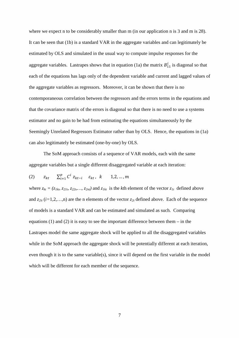
7
where we expect n to be considerably smaller than m (in our application n is 3 and m is 28).
It can be seen that (1b) is a standard VAR in the aggregate variables and can legitimately be
estimated by OLS and simulated in the usual way to compute impulse responses for the
aggregate variables. Lastrapes shows that in equation (1a) the matrix 𝐵𝐵11𝑖𝑖 is diagonal so that
each of the equations has lags only of the dependent variable and current and lagged values of
the aggregate variables as regressors. Moreover, it can be shown that there is no
contemporaneous correlation between the regressors and the errors terms in the equations and
that the covariance matrix of the errors is diagonal so that there is no need to use a systems
estimator and no gain to be had from estimating the equations simultaneously by the
Seemingly Unrelated Regressors Estimator rather than by OLS. Hence, the equations in (1a)
can also legitimately be estimated (one-by-one) by OLS.
The SoM approach consists of a sequence of VAR models, each with the same
aggregate variables but a single different disaggregated variable at each iteration:
(2) 𝑧𝑧𝑘𝑘𝑡𝑡 = ∑ 𝐶𝐶𝑖𝑖 𝑧𝑧𝑘𝑘𝑡𝑡−𝑖𝑖 + 𝜀𝜀𝑘𝑘𝑡𝑡𝑝𝑝𝑖𝑖=1 , 𝑘𝑘 = 1,2, … ,𝑚𝑚
where zkt = (z1kt, z21t, z22t,…, z2nt) and z1kt is the kth element of the vector z1t defined above
and z2it (i=1,2,…,n) are the n elements of the vector z2t defined above. Each of the sequence
of models is a standard VAR and can be estimated and simulated as such. Comparing
equations (1) and (2) it is easy to see the important difference between them – in the
Lastrapes model the same aggregate shock will be applied to all the disaggregated variables
while in the SoM approach the aggregate shock will be potentially different at each iteration,
even though it is to the same variable(s), since it will depend on the first variable in the model
which will be different for each member of the sequence.

8
3. The data
In our application, the aggregate variables will be three GDP variables, one for each
of the three regions, which are defined simply as aggregations of the provinces: the coastal
region, the central region and the western region. This is a common spatial disaggregation of
China and has been used at least since the Seventh Five-Year Plan in 1986. 5 The
disaggregated variables will be provincial GDPs. We therefore require data for real GDP per
capita for each of the provinces and for each of three regions.
All data are annual and are available from 1953 to 2014. We use them in log per
capita terms in 1953 prices. The data are taken from Wu (2004), New China 60 Years
Statistics Compilation (National Statistical Bureau, 2009) and China Statistical Yearbook
(National Statistical Bureau, various issues). We use data for 28 of China’s 31 provinces
(including the “city-provinces” of Beijing, Shanghai and Tianjin), with Chongqing included
in Sichuan, Hainan included in Guangdong and Tibet excluded, all for reasons of missing
data.
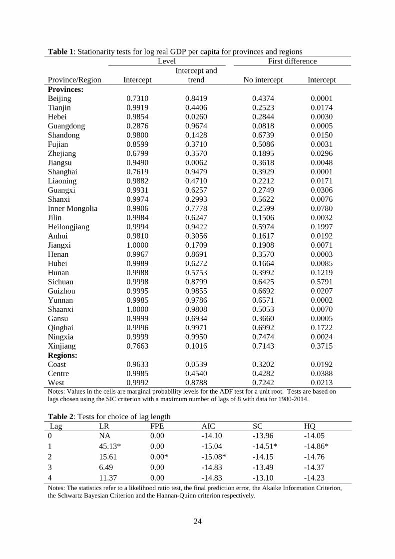
In both approaches which we use it is assumed that the variables are stationary and we
therefore carry out tests of stationarity before proceeding with our empirical analysis. We use
the augmented Dickey-Fuller test and report the results for the (logs of) real GDP per capita
for the provinces and regions in Table 1.
[Table 1 about here]
Clearly most of the variables are I(1) and we follow Lastrapes (2006) and Beckworth (2010)
and work with variables in first differences.
5 The provinces included in the three regions are as follows. Coastal: Beijing, Tianjin, Hebei, Guangdong, Shandong, Fujian, Zhejiang, Jiangsu, Shanghai, Liaoning, Guangxi; Central: Shanxi, Inner Mongolia, Jilin, Heilongjiang, Anhui, Jiangxi, Henan, Hubei, Hunan; Western: Sichuan, Guizhou, Yunnan, Shaanxi, Gansu, Qinghai, Ningxia, Xinjiang. Papers using this classification include Whalley and Zhang (2007), He et al. (2008), Fleisher et al. (2010) and Su and Jefferson (2012).
9
4. Results
4.1 Model specification and estimation
While we have data for the period 1953-2014, we focus on results for a sub-sample,
1980-2014. So much has changed in China since 1953 that it seems implausible to assume
that a model for the full sample could reasonably have stable coefficients over a 60-year
period. Given the important changes in China’s economic direction which began with
“opening-up and reform” in the late 1970s, it seems sensible to begin our sample period at
1980. This also accords with the choice of the start of the sample period in Chen and
Groenewold (2015) and ensures comparability of our results with those in that paper.6
We begin by choosing lag length. We use the same number of lags for each approach
and base it on standard lag-choice criteria for the VAR model in the three regional GDPs.
The results are reported in Table 2. The implications are mixed, with some criteria
suggesting one lag and others two lags. We decided to use two lags; tests for residual
autocorrelation indicated that a model with two lags is free of first- to fourth-order
autocorrelation.
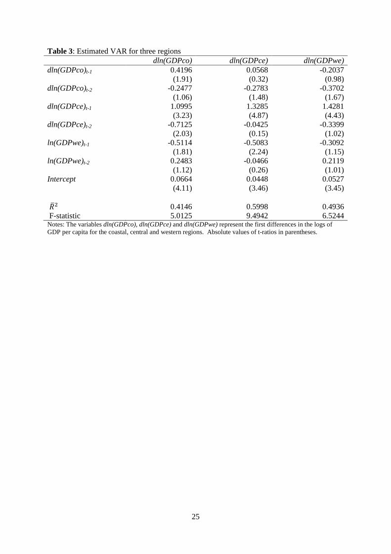
[Tables 2 and 3 about here]
We proceed to the model estimation and start with the Lastrapes approach. Recall that
the estimation strategy for this approach is a two-stage one where we first estimate the VAR
in the three regional variables and then the provincial equations one at a time. The estimated
VAR is reported in Table 3. It is specified in terms of growth rates, calculated as first
differences of the logs of real GDP per capita. The results show that the model has
reasonable explanatory power, especially since the variables are in first-difference form.
There are several significant cross-effects which suggest that there will be significant inter-
regional spillovers of output shocks. This is borne out by the impulse response functions 6 We note, though, that our sample period ends two years later than the one in Chen and Groenewold (2015). Our experimentation with a shorter period ending in 2012 shows that the results are insensitive to the inclusion of these extra two years.
10
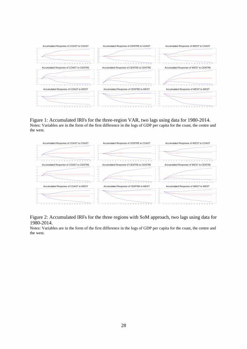
(IRFs) which are shown in Figure 1. These are based on independent unit shocks (chosen for
reasons to be explained below) and reported in accumulated form to convert changes into
levels. All own-effects are significant and positive in the short run and there are significant
spillovers from the centre to both the coast and the west but not from the coast or the west to
the other regions. Surprisingly, the effects of a coastal shock on the other two regions are
small and tend to be negative and the spillovers from the west are larger and also negative.
[Figure 1 about here]
The next step is to generate similar IRFs for the provincial GDP variables. We do this
by feeding the IRF for each of the regional GDP shocks into each of the estimated provincial
equations in turn. The regional IRFs will therefore incorporate the dynamics both in the
regional VAR and in the provincial equations; there will be three sets of provincial IRFs, one
corresponding to each regional shock. Before we can do this, two further modelling
assumptions need to be made. The first concerns the identification of the shocks in the
regional VAR and the second the way in which the regional shocks enter the provincial
equations. With a general specification (subject to the Lastrapes restrictions), each regional
shock will have a potential contemporaneous effects on each other region and on all the
provinces irrespective of which region they are in. This makes it difficult to interpret them as
regional shocks; if, for example, a coastal shock has a contemporaneous effect on all
provinces irrespective of which region they are in, to what extent is it a coastal shock? We
therefore impose two further restrictions; first, that in the VAR part of the model each
regional shock has a contemporaneous effect only on its own region (independent shocks)
and, second, consistently with this, that each regional shock feeds through
contemporaneously only to the provinces in that region. Spillovers into other regions and
other provinces are possible but occur only with a lag.
11
We make similar assumptions for the SoM approach – a lag length of two and similar
shock identification. In particular, in each model iteration it is assumed that a regional shock
does not contemporaneously affect the provinces in the other regions but has an immediate
effect on provincial output only if the province lies within the region itself. The regional
IRFs will differ with each iteration of the model. To provide a comparison of the regional
IRFs for the SoM case to those derived from the Lastrapes approach reported in Figure 1, we
average the regional IRFs across the 28 model iterations and show them in Figure 2. They
are clearly very similar to those generated by the three-variable VAR which are reported in
Figure 1.
[Figure 2 about here]
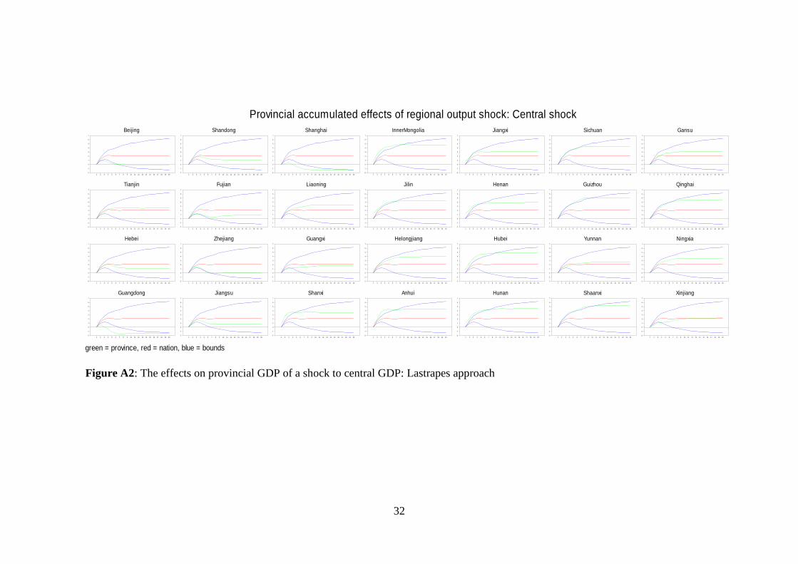
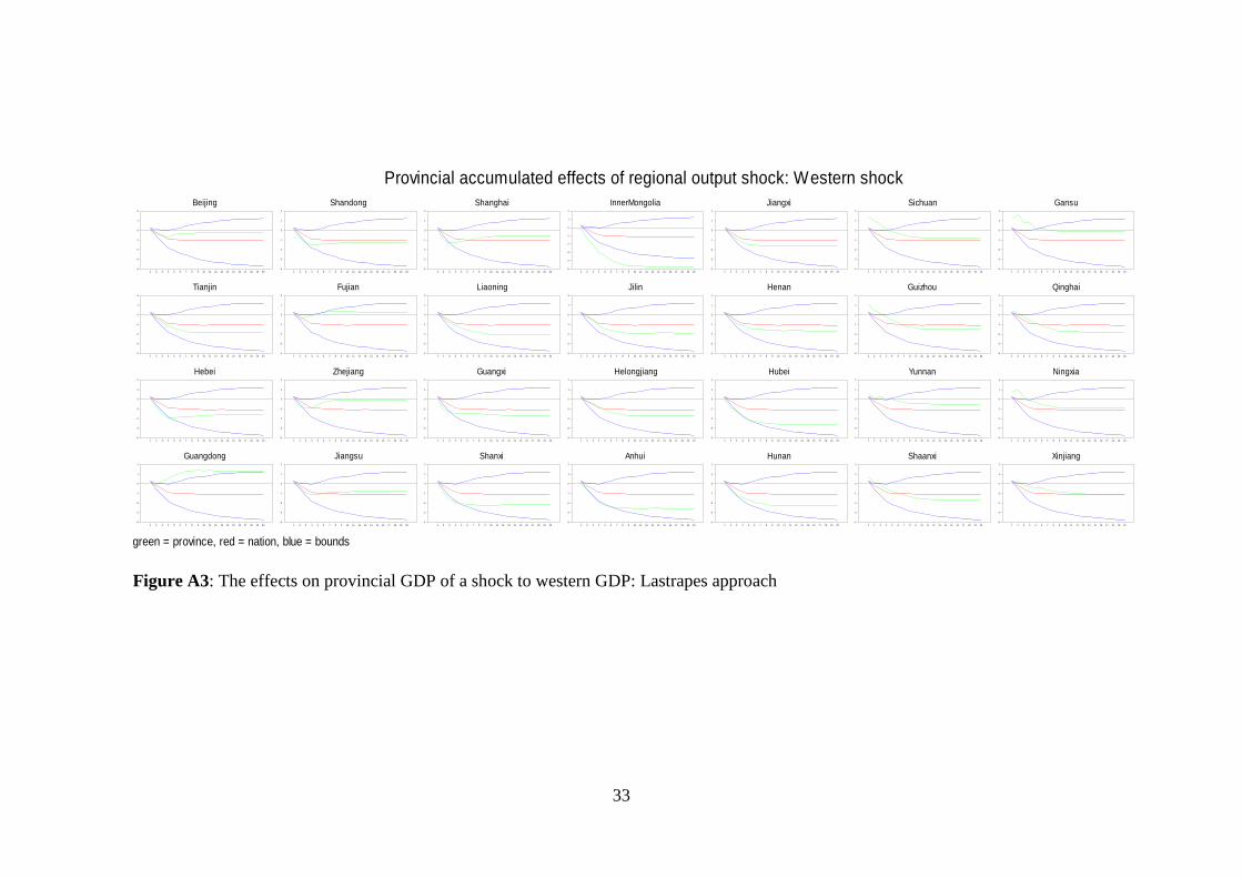
The provincial IRFs derived from the Lastrapes approach are reported in Figures A1
to A3 in the Appendix, and those generated by the SoM approach are shown in Figures A4 to
A6 in the Appendix. In each case, in order to facilitate the comparison of effects across
provinces, we compare each provincial IRF to the national IRF and include the national
confidence bounds to provide a measure of significance of the deviation of the provincial IRF
from its national counterpart.7
The individual provincial IRFs contain a lot of information; to ease interpretation, we
summarise this by characterising the relationship between the provincial IRF and the national
IRF at two forecast horizons which we call “short run” (one period after the shock) and “long
run” (nine periods after the shock).8 We denote IRFs which are above (below) the national
IRF by “A” (“B”) and we use a “C” designation for an IRF which is approximately
7 Neither model generates national IRFs and bounds. We have computed these as weighted averages of the three regional IRFs and bounds with weights equal to shares of national output averaged over 1982-2014. For the SoM approach the regional IRFs and bounds are the averages across all 28 model iterations. 8 In the IRFs in the Appendix the horizons are numbered such that the shock occurs at t=1; then t=2 is one period after the shock and t=10 is nine periods after the shock. Nothing much changes to the overall characterisation of the results if we make the long run shorter than 9 periods, say, 5 periods after the shock.
12
coincident with its national counterpart.9 We follow the approach of Fraser et al. (2014) and
call a provincial effect significantly different from the national IRF if it lies outside the
national confidence bounds and in the tables reported below we use an asterisk to indicate
significance in this sense. We will discuss the provincial responses in detail in the following
sub-sections.
4.2 The effects of a regional shock on the provinces: Lastrapes model
The effects on all 28 provinces of the three regional shocks under the assumptions of
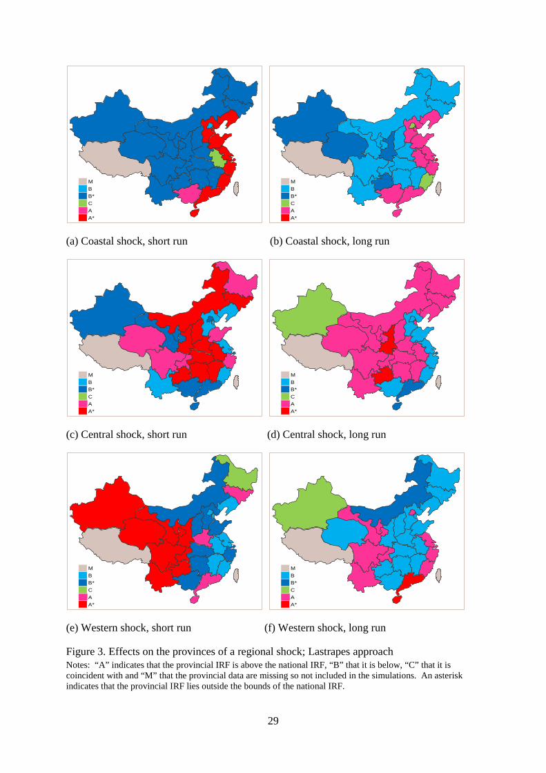
the Lastrapes model are summarised in Table 4 and pictured in maps in Figure 3.
[Table 4 about here]
[Figure 3 about here]
4.2.1 The effects of a shock to the coast
Consider the effects on the provinces of a shock to the coastal region first. The most
striking feature of the results in the first two columns of Table 4 is that, in the short run, the
effects are concentrated in the coastal provinces. Almost all provinces in the coastal region
experience an effect which is significantly above the national average while the provinces in
the other two regions perform significantly below the national average. To some extent, this
is driven by our modelling assumptions that the coastal shock has a contemporaneous effect
only on the provinces in that region so that the short-run effects incorporate only one period’s
potential spillovers into the other regions. The effects of a coastal shock are graphically
illustrated in the maps in Figures 3(a) and 3(b) which capture the information in the first two
columns of Table 4. They, too, show a stark divide between the coast and the remainder of
the country. Two exceptions stand out: Beijing and Anhui. Of all the coastal provinces, only
Beijing experiences a below-average effect in the short run and Anhui is the only non-coastal 9 In particular, we say that the provincial and national IRFs are coincident at a particular horizon if the provincial IRF lies within 5% of the distance between the national confidence bounds on either side of the national IRF at that horizon.
13
province which does not show a below average effect, closely mimicking the average for the
nation as a whole.
The general characterisation of the effects, as shown in Table 4 and pictured in
Figures 3(a) and 3(b), does not change much when we move from the short to the long run.
After nine periods the effects of a shock to coastal GDP are still concentrated in the coastal
provinces with most of them experiencing an above-average effect while most of the non-
coastal provinces show an effect which is below the national average. Far fewer of the
differences are significant in the long run, however, but this reflects the wider confidence
bounds as well as some convergence of the coastal provincial IRFs to the national average as
can be seen from an inspection of Figure A1 in the Appendix.
The summary information contained in Table 4 and pictured in Figures 3(a) and 3(b)
is informative but does hide some of the more detailed information available in the individual
provincial IRFs in Figure A1. It is clear that, on the whole, the provinces within a region
respond similarly to the region as a whole as shown in Figure 1. The provincial IRFs show
several interesting additional aspects of the results. First, it is clear that Beijing closely
follows the national IRFs, suggesting that of all the coastal provinces, Beijing is disconnected
from its region and more aligned with China as a whole. This has recently been recognised
by the Chinese central government when it implemented a programme to better integrate
Beijing into the economies of its neighbours, Tianjin and Hebei – the so-called “Jing-Jin-Ji
Integration Policy”. Another interesting feature of the individual IRFs is the very strong
performance of Shanghai which begins significantly above the national average and increases
its deviation from the national IRFs over time. Further, a group of coastal provinces
(Guangdong, Zhejiang, Fujian and Jiangsu) start off very strongly, initially increasing their
deviation from the national average, but begin to converge to the average after about three
periods.
14
Turning to the non-coastal provinces, the individual IRFs show an interesting
distinction between central and western provinces. While the summary information in Table
4 and the maps show that all non-coastal provinces experience an effect which is below the
national average, the individual IRFs show that for the western provinces this effect is
actually generally negative while the central provinces receive small positive effects, with
this positive effect tending to be concentrated in the provinces nearer the coast – Anhui,
Jiangxi, Henan, Hubei and Hunan. Thus over time there are small beneficial spillovers to
most of the central provinces but the western provinces actually suffer a fall in GDP
following a coastal boost.
All in all then, economic stimulus which originates in the coastal region generally
benefits the coastal provinces more than the non-coastal provinces in both the short run and
the long run. There are only weak positive spillovers to the central provinces over time and
these beneficial spillovers tend to be concentrated in the provinces nearest the coast. The
western provinces actually experience negative spillovers – their GDPs decline as a result of
the coastal boost.
4.2.2 The effects of a shock to the centre
The detailed provincial IRFs following a shock to the central region are in Figure A2
in the Appendix while the effects are summarised in the third and fourth columns in Table 4
and the maps in Figure 3(c) and 3(d). It is clear from the information in Table 4 and in the
maps that there are strong similarities to the results for the coastal shock – the effects of the
central shock are felt mainly in the central region itself, especially in the short run: all central
provinces experience an above-average effect and all are significant except for Heilongjiang,
the geographically most distant of the central provinces. In contrast to the coastal effects,
however, there are significant short-run spillovers to provinces in the other two regions. This
is particularly true for the western region and is consistent with the regional IRFs in Figure 1.

15
In the coast only two provinces (Shandong and Zhejiang) receive short-run spillovers and,
from the individual IRFs in Figure A1, it is clear that they are small and disappear quickly.
The spillovers to the west, however, are more significant and long-lasting: one half of the
western provinces (Sichuan, Guizhou, Shaanxi and Qinghai) perform strongly and
consistently above the national average following a central shock. Shaanxi and Guizhou may
be explained by their contiguity to the central region and may, therefore, be closely integrated
with it. But Qinghai and, to a lesser extent, Sichuan, are more distant from the centre and
therefore more difficult to rationalise. Finally, in contrast to the effects of a coastal shock,
relatively few provinces actually respond negatively to the central shock; in fact, only the
coastal provinces of Guangdong (which includes Hainan) and Shanghai have significant and
negative long-run responses to the boost in output in the central region.
4.2.3 The effects of a shock to the west
Consider next the responses of the provincial economies to a shock to the western
region, the individual IRFs for which are reported in Figure A3 in the Appendix with the
summary results in the last two columns of Table 4 and Figures 3(e) and 3(f). In the short run
the results show similar characteristics to the previous two shocks – the provinces in the
region where the shock originates experience an above-average effect whereas most of the
remaining provinces perform below-average. There are some exceptions to this general result:
Guangdong in the coastal region and Jilin and Henan in the central region all show an above-
average effects of a western shock. Over time there are interesting changes, as can be seen
when comparing the short- and long-run results in the table and the maps: the above-average
results in the centre weaken considerably but there is a distinct shift of the effects to the coast
– six of the 11 coastal provinces exhibit an above-average effect. Thus we might conclude
that there is some positive spillover of the shock to the central provinces in the short run but
substantial spillover to the coast in the long run. Moreover, the beneficial effects on the
16
western provinces themselves dissipate over time since only one half of the western
provinces experience an above-average effect in the long run. The interpretation of the
effects of a western shock are complicated, however, when we look at the individual
provincial IRFs in Figure A3 in the Appendix. This shows that the national effect of a
western shock is negative after the period in which the shock occurs and is consistent with the
regional effects pictured in Figure 1. This being the case, an above-average effect may still
be (and often is) a negative one. Moreover, it is clear that the majority of the western
provinces lose ground over time while many of the coastal provinces gain ground, with some
such as Guangdong and Fujian becoming positive in the long run. Central provinces are all
consistently below the national average in the short run and become more negative over time
even though some become insignificant (but this reflects the widening confidence bounds).
We can draw clear conclusions from these empirical results which follow the
application of the Lastrapes method. First, the effects of a regional shock fall mainly on the
provinces in the region itself, especially in the short run. There is, therefore, little evidence of
short-run spillovers. This effect is, however, more marked for the coast than it is for the other
two regions. Over time there is some spread of effects to provinces in the other regions
although, again, there is less evidence of this for a coastal shock. In the case of a central
shock there are substantial spillovers to the western provinces while there is a distinct shift
from the west to the coast following a western shock.
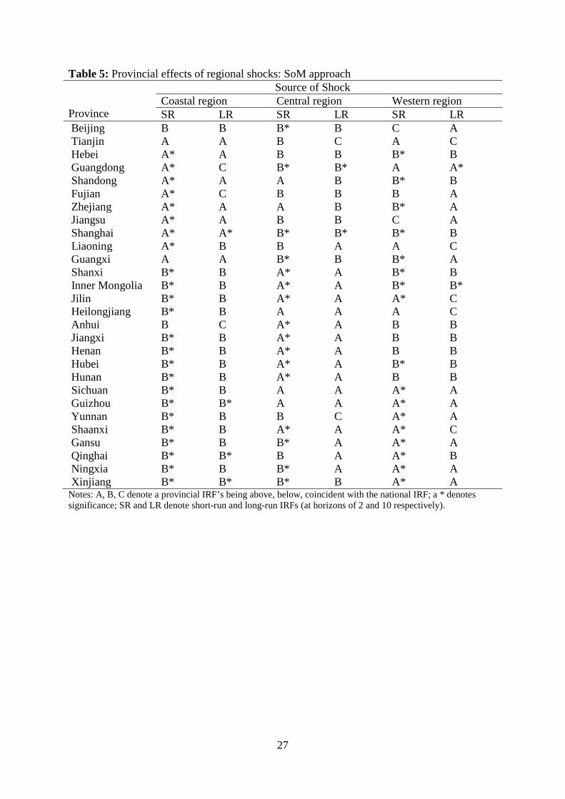
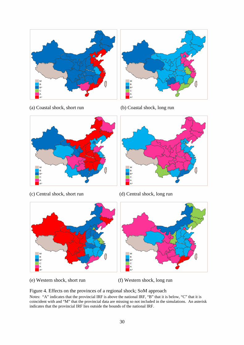
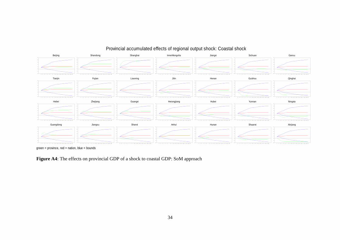
4.3 The effects of a regional shock on the provinces: SoM approach
Our second approach is to estimate and simulate a sequence of VAR models, each of
which has all three regional variables in it supplemented by a single provincial variable, each
member of the sequence taking a different provincial variable. There are, therefore, 28
iterations of the model. The resulting IRFs for the 28 provinces together with the national
17
IRF and its bounds are reported in the Appendix, Figures A4 to A6. The results are
summarised in Table 5 and in maps in Figure 4.
[Table 5 about here]
[Figure 4 about here]
It is clear from a comparison of the individual provincial IRFs in Figures A4 to A6 to their
counterparts in Figure A1 to A3 that there are differences in individual IRFs but that these are
generally differences of degree rather than differences of kind. Thus, the provincial IRFs
generally lie on the same side of the national average no matter which approach is used to
generate them. Moreover, they are also generally on the same side of the confidence bounds.
This similarity is also apparent from the characterisation in Table 5 and Figure 4. The
Lastrapes result, discussed in the previous sub-section, that the effects of a coastal shock are
largely restricted to the coastal provinces continues to hold for the SoM-based IRFs. In the
case of a central shock, the limitation of the effects to the central provinces is more marked, if
anything, for the SoM-based IRFs. The opposite is true of the effects of a western shock,
spillovers from which are somewhat more marked in the SoM-based IRFs, particularly
spillovers to the north-eastern provinces of Liaoning, Jilin and Heilongjiang.
All in all, then, we can conclude that the results obtained using the SoM approach are
remarkably similar to those generated by the Lastrapes model. Therefore, on the one hand,
the effects estimated under Lastrapes’ assumptions are robust to the choice of model. On the
other hand, the common objection to the use of the SoM procedure (that potentially different
aggregate shocks are applied to each province) seems not to be serious, at least in this
particular application.
18
5. Conclusions
In this paper we have examined the effects at the provincial level in China of shocks
at the regional level, with three regions (coast, centre and west) being distinguished. We used
two different approaches: a restricted VAR model, based on a procedure developed in
Lastrapes (2005) and a sequence of models as applied by Carlino and DeFina (1998, 1999).
The Lastrapes approach has been used in the analysis of the provincial effects of national
shocks previously in Chen and Groenewold (2015); we extended their analysis by focussing
on the regional source of shocks as well as providing a comparison to the sequence-of-models
(SoM) procedure.
Clear conclusions emerge from the analysis. First, the overall conclusions are not
greatly affected by the method used. This provides some counter-balance to the criticism of
the SoM method as well as to the possible concerns with the strong assumptions used to
achieve tractability in the Lastrapes approach.
As to the effects as such, we found, first, that in the short run a shock to a particular
region had above-average effects on the provinces in the region being shocked and below-
average effects elsewhere in the country. This was particularly strong for a shock originating
in the coastal region. There were, therefore, few short-run spillovers into provinces in other
regions. Second, over time there was some spread of the effects to provinces in other regions
although, again, this was less so for a coastal shock than for shocks to the other two regions.
In particular, for the coastal shock there were few spillovers over time, for a central shock
there were some spillovers into the western provinces and for a western shock there was a
marked shift in activity from the west to the coastal provinces over time after the shock.
Finally, we return to one of the motivating arguments for this study and consider
some implications of the results for the relationship between aggregate/regional policy and
inter-provincial disparities. First, the effect of an aggregate shock on inter-provincial

19
disparities depends on the region in which the shock occurs. Thus, if policy-makers are
concerned about the effects of their actions on the inequalities across provinces, the region in
which the policy is focussed will need to be carefully considered. Second, if national growth
is boosted by policy which initially benefits mainly the coast (as has often been the case in
the period since opening-up in the 1980s), the beneficial effects will be felt mainly in the
coastal provinces with little diffusion to the rest of the country. This will serve to exacerbate
existing inequalities.10 Third, a shock which increases output originating in the central region
will be felt in the short turn mainly in the centre and so reduce disparities between the centre
and the coast but widen them between the centre and the west although this latter effect will
weaken over time as there is some spillover to the west. Finally, if the western region is the
focus of policy, the gap between the west and the rest of the country will narrow in the short
run but as time passes much of the benefit will spread to the coast which will offset the
original narrowing of disparities.11 Thus, overall, the results suggest that it is difficult to
design policy which will promote growth and reduce the extent to which the west lags the rest
of the country. Certainly, policy-makers will need to be aware of the possible negative
effects on equality of regionally-focussed policy when they decide which regions are to be
targeted and, also, whether they have a short- or long-run focus.
10 For a similar finding but related to the effect on the rural-urban divide of boosting large cities see Chen and Partridge (2013). 11 See Groenewold et al. (2010) for a similar finding that “at least part of the expenditure boosts in the poorer inland regions find their way to the coastal provinces” (p.87). Similarly, Herrerias and Monfort (2015) argue that coastal provinces have benefitted most from economic growth and there is a danger that such policies “have created small regional clusters” (p.485) of provinces with very different levels of income. Tian et al.(2016) express a similar view and provide supporting evidence.
20
References
Abdallah, C. S and W. D. Lastrapes. 2013. Evidence on the relationship between housing and
consumption in the United States: A state-level analysis. Journal of Money, Credit
and Banking, 45, 559-589.
Andersson, F. N. G., D. L. Edgerton and S. Opper. 2013. A matter of time: Revisiting growth
convergence in China. World Development, 45, 239-251..
Bai, C., H. Ma and W. Pan. 2012. Spatial spillover and regional economic growth in China.
China Economic Review, 23, 982-990.
Beckworth, D. 2010. One nation under the Fed? The asymmetric effects of US monetary
policy and its implications for the United States as an optimal currency area. Journal
of Macroeconomics, 32, 732–746.
Carlino, G. and R. DeFina. 1998. The differential regional effects of monetary policy. Review
of Economics and Statistics, 80, 572-587.
Carlino, G. and R. DeFina. 1999. The differential regional effects of monetary policy:
Evidence from the U.S. states. Journal of Regional Science, 39, 339-358.
Cevik, S. and C. Correa-Caro. 2015. Growing (un)equal: Fiscal policy and income inequality
in China and BRIC+. IMF Working Paper WP/15/68.
Chan, K. S., X. Zhou and Z. Pan. 2014. The growth and inequality nexus: The case of China.
International Review of Economics and Finance, 34, 230–236
Chen, A. 2010. Reducing China's regional disparities: Is there a growth cost? China
Economic Review, 21, 2-13.
Chen, A and N. Groenewold. 2015. The regional effects of macroeconomic shocks in China.
China Economic Review, forthcoming.
Chen, A. and M. D. Partridge. 2013. When are cities engines of growth in China? Spread and
backwash effects across the urban hierarchy. Regional Studies, 47, 1313-1331.
Chen, Z. 2013. The political economy of urban and rural development in China. In M. Lu, Z.
Chen, X. Zhu and X. Xu (eds.). China’s Regional Development, London and New
York: Routledge, 92-133.
Cunha Neves, P. and S. M.Tavares Silva. 2014. Inequality and growth: Uncovering the main
conclusions from the empirics. Journal of Development Studies, 50, 1-21.
Fleisher B., Li, H. and Zhao, M. 2010. Human Capital, Economic Growth, and Regional
Inequality in China. Journal of Development Economics, 92: 215-231.
21
Fraser, P., G. A. Macdonald and A. W. Mullineux. 2014. Regional monetary policy: An
Australian perspective. Regional Studies, 48, 1419-1433.
Groenewold, N., A. Chen and G. Lee. 2008. Linkages between China’s Regions:
Measurement and Policy. Cheltenham, UK: Edward Elgar.
Groenewold, N., A. Chen and G. Lee. 2010. Inter-regional spillovers of policy shocks in
China. Regional Studies, 44, 87-101.
Gu, X. and P. S Tam. 2013. The saving-growth-inequality triangle in China. Economic
Modelling, 33, 850-857.
He, C., Y. D. Wei and X. Xie. 2008. Globalization, institutional change, and industrial
location: Economic transition and industrial concentration in China. Regional Studies,
42, 923-945.
Herrerias, M.J. and J. O. Monfort. 2015. Testing stochastic convergence across Chinese
provinces. Regional Studies, 49, 485-501.
Hirschman, A. 1958. The Strategy of Economic Development. New Haven: Yale University
Press.
Knight, J. 2008. Reform, growth and inequality in China. Asian Economic Policy Review, 3,
140-158.
Knight, J. 2016. The societal cost of China's rapid economic growth. Asian Economic Papers,
15, 138-59
Kraay, A. 2015. Weak instruments in growth regressions: Implications for recent cross-
country evidence on inequality and growth. World Bank Policy Research Working
Paper WPS7494.
Kuijs, L. and T. Wang. 2005. China's pattern of growth: Moving to sustainability and
reducing inequality. World Bank China Research Paper, No.2.
Kuznets, S. 1955. Economic growth and income inequality. American Economic Review, 45,
1-28.
Lastrapes, W. D. 2005. Estimating and identifying vector autoregressions under diagonality
and block exogeneity restrictions. Economics Letters, 87, 75–81.
Lastrapes, W. D. 2006. Inflation and the distribution of relative prices: the role of
productivity and money supply shocks. Journal of Money, Credit, and Banking, 38,
2159–2198.
Lemoine, F., G. Mayo, S. Poncet and D. Unal. 2014. The geographic pattern of China's
growth and convergence within industry. CEPII Research Center, Working Paper.
22
Li, T. J. Lai, Y. Wang and D. Zhao. 2016. Long-run relationship between inequality and
growth in post-reform China: New evidence from dynamic panel model. International
Review of Economics and Finance, 41, 238-52
Lopez-Bazo, E., V. Monastiriotis and R. Ramos. 2014. Spatial inequalities and economic
growth: Editorial. Spatial Economic Analysis, 9, 113-119.
Lyhagen, J. and J. Rickne. 2014. Income inequality between Chinese regions: newfound
harmony or continued discord? Empirical Economics, 47, 93-110.
Myrdal, G. 1957. Economic Theory and Underdeveloped Regions. London: Duckworth.
National Statistical Bureau. 2009. New China 60 Years Statistics Compilation. Beijing:
Statistical Publishing House of China.
National Statistical Bureau. various issues. China Statistical Yearbook. Beijing: Statistical
Publishing House of China.
Qiao, B, J. Martinez-Vazquez and Y. Xu. 2008. The trade-off between growth and equity in
decentralisation policy: China’s experience. Journal of Development Economics, 86,
112-128.
Risso, W. A. and E. J. Sanchez Carrera. 2012. Inequality and economic growth in China.
Journal of Chinese Economic and Foreign Trade Studies, 5, 80-90.
Su, J. and G. H. Jefferson. 2012. Differences in returns to FDI between China's coast and
interior: One country, two economies? Journal of Asian Economics, 23, 259-269.
Tian, X., X. Zhang, Y. Zhou and X. Yu. 2016. Regional income inequality in China revisited:
A perspective from club convergence. Economic Modelling, 56, 50-58.
Wan G., M. Lu and Z. Chen. 2006. The inequality-growth nexus in the short and long run:
Empirical evidence from China. Journal of Comparative Economics, 34, 654-667.
Whalley, J. and S. Zhang. 2007. A numerical simulation analysis of (Hukou) labour mobility
restrictions in China. Journal of Development Economics, 83, 392-410.
Williamson, J. 1965. Regional inequality in the process of national development. Economic
Development and Cultural Change, 17, 3-84.
Wong, J. 2006. China’s economy in 2005: At a new turning point and need to fix its
development problems. China & World Economy, 14, 1-15.
Wu, Y. 2004. China's Economic Growth: A Miracle with Chinese Characteristics. London:
Routledge Curzon.
Wu, Y. and H. Yao. 2015. Income inequality, state ownership, and the pattern of economic
growth – A tale of the Kuznets curve for China since 1978. Atlantic Economic
Journal, 43, 165-180.
23
Xu, X., X. Wang and Y. Gao. 2013. The political economy of regional development in China.
In M. Lu, Z. Chen, X. Zhu and X. Xu (eds.). China’s Regional Development, London
and New York: Routledge, 41-90.
Zhao, X. B. and S. P. Tong. 2000. Unequal economic development in China: Spatial
disparities and regional policy reconsideration. Regional Studies, 34, 549-561.
Zheng, D. and T. Kuroda. 2013. The role of public infrastructure in China’s regional
inequality and growth: A simultaneous equations approach. The Developing
Economies, 51, 79-107.
Zhu, C. and G. Wan. 2012. Rising inequality in China and the move to a balanced economy.
China & World Economy, 20, 83-104.
24
Table 1: Stationarity tests for log real GDP per capita for provinces and regions
Province/Region
Level First difference
Intercept Intercept and
trend
No intercept Intercept Provinces: Beijing 0.7310 0.8419 0.4374 0.0001 Tianjin 0.9919 0.4406 0.2523 0.0174 Hebei 0.9854 0.0260 0.2844 0.0030 Guangdong 0.2876 0.9674 0.0818 0.0005 Shandong 0.9800 0.1428 0.6739 0.0150 Fujian 0.8599 0.3710 0.5086 0.0031 Zhejiang 0.6799 0.3570 0.1895 0.0296 Jiangsu 0.9490 0.0062 0.3618 0.0048 Shanghai 0.7619 0.9479 0.3929 0.0001 Liaoning 0.9882 0.4710 0.2212 0.0171 Guangxi 0.9931 0.6257 0.2749 0.0306 Shanxi 0.9974 0.2993 0.5622 0.0076 Inner Mongolia 0.9906 0.7778 0.2599 0.0780 Jilin 0.9984 0.6247 0.1506 0.0032 Heilongjiang 0.9994 0.9422 0.5974 0.1997 Anhui 0.9810 0.3056 0.1617 0.0192 Jiangxi 1.0000 0.1709 0.1908 0.0071 Henan 0.9967 0.8691 0.3570 0.0003 Hubei 0.9989 0.6272 0.1664 0.0085 Hunan 0.9988 0.5753 0.3992 0.1219 Sichuan 0.9998 0.8799 0.6425 0.5791 Guizhou 0.9995 0.9855 0.6692 0.0207 Yunnan 0.9985 0.9786 0.6571 0.0002 Shaanxi 1.0000 0.9808 0.5053 0.0070 Gansu 0.9999 0.6934 0.3660 0.0005 Qinghai 0.9996 0.9971 0.6992 0.1722 Ningxia 0.9999 0.9950 0.7474 0.0024 Xinjiang 0.7663 0.1016 0.7143 0.3715 Regions: Coast 0.9633 0.0539 0.3202 0.0192 Centre 0.9985 0.4540 0.4282 0.0388 West 0.9992 0.8788 0.7242 0.0213 Notes: Values in the cells are marginal probability levels for the ADF test for a unit root. Tests are based on lags chosen using the SIC criterion with a maximum number of lags of 8 with data for 1980-2014. Table 2: Tests for choice of lag length Lag LR FPE AIC SC HQ 0 NA 0.00 -14.10 -13.96 -14.05 1 45.13* 0.00 -15.04 -14.51* -14.86* 2 15.61 0.00* -15.08* -14.15 -14.76 3 6.49 0.00 -14.83 -13.49 -14.37 4 11.37 0.00 -14.83 -13.10 -14.23 Notes: The statistics refer to a likelihood ratio test, the final prediction error, the Akaike Information Criterion, the Schwartz Bayesian Criterion and the Hannan-Quinn criterion respectively.
25
Table 3: Estimated VAR for three regions
dln(GDPco) dln(GDPce) dln(GDPwe)
dln(GDPco)t-1 0.4196 0.0568 -0.2037
(1.91) (0.32) (0.98)
dln(GDPco)t-2 -0.2477 -0.2783 -0.3702
(1.06) (1.48) (1.67)
dln(GDPce)t-1 1.0995 1.3285 1.4281 (3.23) (4.87) (4.43) dln(GDPce)t-2 -0.7125 -0.0425 -0.3399 (2.03) (0.15) (1.02) ln(GDPwe)t-1 -0.5114 -0.5083 -0.3092 (1.81) (2.24) (1.15) ln(GDPwe)t-2 0.2483 -0.0466 0.2119 (1.12) (0.26) (1.01) Intercept 0.0664 0.0448 0.0527 (4.11) (3.46) (3.45) 𝑅𝑅�2 0.4146 0.5998 0.4936 F-statistic 5.0125 9.4942 6.5244 Notes: The variables dln(GDPco), dln(GDPce) and dln(GDPwe) represent the first differences in the logs of GDP per capita for the coastal, central and western regions. Absolute values of t-ratios in parentheses.

26
Table 4: Provincial effects of regional shocks: Lastrapes approach Province
Source of Shock Coastal region Central region Western region SR LR SR LR SR LR
Beijing B C B* B B A Tianjin A* A B A B B Hebei A* A B B B* B Guangdong A* A B* B* A A* Shandong A* A A B B* B Fujian A* C B B B A Zhejiang A* A A B B* A Jiangsu A* A B B B A Shanghai A* A* B* B* B* A Liaoning A* A B A B B Guangxi A A B* B B* B Shanxi B* B A* A B* B Inner Mongolia B* B A* A B* B* Jilin B* B A* A A B Heilongjiang B* B A A C B Anhui C A A* A B B Jiangxi B* B A* A B B Henan B* B A* A A B Hubei B* B A* A B* B Hunan B* B A* A B* B Sichuan B* B A A A* A Guizhou B* B* A* A* A* B Yunnan B* B B A A* A Shaanxi B* B* A* A* A* B Gansu B* B B* A A* A Qinghai B* B* A A A* B Ningxia B* B B* A A* A Xinjiang B* B* B* C A* C Notes: A, B, C denote a provincial IRF’s being above, below, coincident with the national IRF; a * denotes significance; SR and LR denote short-run and long-run IRFs (at horizons of 2 and 10 respectively).
27
Table 5: Provincial effects of regional shocks: SoM approach Province
Source of Shock Coastal region Central region Western region SR LR SR LR SR LR
Beijing B B B* B C A Tianjin A A B C A C Hebei A* A B B B* B Guangdong A* C B* B* A A* Shandong A* A A B B* B Fujian A* C B B B A Zhejiang A* A A B B* A Jiangsu A* A B B C A Shanghai A* A* B* B* B* B Liaoning A* B B A A C Guangxi A A B* B B* A Shanxi B* B A* A B* B Inner Mongolia B* B A* A B* B* Jilin B* B A* A A* C Heilongjiang B* B A A A C Anhui B C A* A B B Jiangxi B* B A* A B B Henan B* B A* A B B Hubei B* B A* A B* B Hunan B* B A* A B B Sichuan B* B A A A* A Guizhou B* B* A A A* A Yunnan B* B B C A* A Shaanxi B* B A* A A* C Gansu B* B B* A A* A Qinghai B* B* B A A* B Ningxia B* B B* A A* A Xinjiang B* B* B* B A* A Notes: A, B, C denote a provincial IRF’s being above, below, coincident with the national IRF; a * denotes significance; SR and LR denote short-run and long-run IRFs (at horizons of 2 and 10 respectively).
28
Figure 1: Accumulated IRFs for the three-region VAR, two lags using data for 1980-2014. Notes: Variables are in the form of the first difference in the logs of GDP per capita for the coast, the centre and the west.
Figure 2: Accumulated IRFs for the three regions with SoM approach, two lags using data for 1980-2014. Notes: Variables are in the form of the first difference in the logs of GDP per capita for the coast, the centre and the west.
Accumulated Response of COAST to COAST
1 2 3 4 5 6 7 8 9 10 11 12 13 14 15 16 17 18 19 20-1
0
1
2
3
4
Accumulated Response of COAST to CENTRE
1 2 3 4 5 6 7 8 9 10 11 12 13 14 15 16 17 18 19 20-3
-2
-1
0
1
2
3
4
5
Accumulated Response of COAST to WEST
1 2 3 4 5 6 7 8 9 10 11 12 13 14 15 16 17 18 19 20-4
-3
-2
-1
0
1
2
Accumulated Response of CENTRE to COAST
1 2 3 4 5 6 7 8 9 10 11 12 13 14 15 16 17 18 19 20-2.0
-1.5
-1.0
-0.5
0.0
0.5
1.0
1.5
2.0
2.5
Accumulated Response of CENTRE to CENTRE
1 2 3 4 5 6 7 8 9 10 11 12 13 14 15 16 17 18 19 200
2
4
6
8
10
Accumulated Response of CENTRE to WEST
1 2 3 4 5 6 7 8 9 10 11 12 13 14 15 16 17 18 19 20-6
-5
-4
-3
-2
-1
0
1
Accumulated Response of WEST to COAST
1 2 3 4 5 6 7 8 9 10 11 12 13 14 15 16 17 18 19 20-3
-2
-1
0
1
2
Accumulated Response of WEST to CENTRE
1 2 3 4 5 6 7 8 9 10 11 12 13 14 15 16 17 18 19 200
1
2
3
4
5
6
7
8
9
Accumulated Response of WEST to WEST
1 2 3 4 5 6 7 8 9 10 11 12 13 14 15 16 17 18 19 20-4
-3
-2
-1
0
1
2
Accumulated Response of COAST to COAST
1 2 3 4 5 6 7 8 9 10 11 12 13 14 15 16 17 18 19 20-1
0
1
2
3
4
5
Accumulated Response of COAST to CENTRE
1 2 3 4 5 6 7 8 9 10 11 12 13 14 15 16 17 18 19 20-4
-2
0
2
4
6
Accumulated Response of COAST to WEST
1 2 3 4 5 6 7 8 9 10 11 12 13 14 15 16 17 18 19 20-5
-4
-3
-2
-1
0
1
2
3
Accumulated Response of CENTRE to COAST
1 2 3 4 5 6 7 8 9 10 11 12 13 14 15 16 17 18 19 20-3
-2
-1
0
1
2
3
4
Accumulated Response of CENTRE to CENTRE
1 2 3 4 5 6 7 8 9 10 11 12 13 14 15 16 17 18 19 200
2
4
6
8
10
12
Accumulated Response of CENTRE to WEST
1 2 3 4 5 6 7 8 9 10 11 12 13 14 15 16 17 18 19 20-7
-6
-5
-4
-3
-2
-1
0
1
Accumulated Response of WEST to COAST
1 2 3 4 5 6 7 8 9 10 11 12 13 14 15 16 17 18 19 20-4
-3
-2
-1
0
1
2
3
Accumulated Response of WEST to CENTRE
1 2 3 4 5 6 7 8 9 10 11 12 13 14 15 16 17 18 19 20-2
0
2
4
6
8
10
12
Accumulated Response of WEST to WEST
1 2 3 4 5 6 7 8 9 10 11 12 13 14 15 16 17 18 19 20-6
-5
-4
-3
-2
-1
0
1
2
3
29
(a) Coastal shock, short run (b) Coastal shock, long run
(c) Central shock, short run (d) Central shock, long run
(e) Western shock, short run (f) Western shock, long run
Figure 3. Effects on the provinces of a regional shock; Lastrapes approach Notes: “A” indicates that the provincial IRF is above the national IRF, “B” that it is below, “C” that it is coincident with and “M” that the provincial data are missing so not included in the simulations. An asterisk indicates that the provincial IRF lies outside the bounds of the national IRF.
MBB*CAA*
MBB*CAA*
MBB*CAA*
MBB*CAA*
MBB*CAA*
MBB*CAA*
30
(a) Coastal shock, short run (b) Coastal shock, long run
(c) Central shock, short run (d) Central shock, long run
(e) Western shock, short run (f) Western shock, long run
Figure 4. Effects on the provinces of a regional shock; SoM approach Notes: “A” indicates that the provincial IRF is above the national IRF, “B” that it is below, “C” that it is coincident with and “M” that the provincial data are missing so not included in the simulations. An asterisk indicates that the provincial IRF lies outside the bounds of the national IRF.
MBB*CAA*
MBB*CAA*
MBB*CAA*
MBB*CAA*
MBB*CAA*
MBB*CAA*
31
Appendix
Figure A1: The effects on provincial GDP of a shock to coastal GDP: Lastrapes approach
Provincial accumulated effects of regional output shock: Coastal shock
green = province, red = nation, blue = bounds
Beijing
1 2 3 4 5 6 7 8 9 10 11 12 13 14 15 16 17 18 19 20-2
-1
0
1
2
3
4
Tianjin
1 2 3 4 5 6 7 8 9 10 11 12 13 14 15 16 17 18 19 20-2
-1
0
1
2
3
4
Hebei
1 2 3 4 5 6 7 8 9 10 11 12 13 14 15 16 17 18 19 20-2
-1
0
1
2
3
4
Guangdong
1 2 3 4 5 6 7 8 9 10 11 12 13 14 15 16 17 18 19 20-2
-1
0
1
2
3
4
Shandong
1 2 3 4 5 6 7 8 9 10 11 12 13 14 15 16 17 18 19 20-2
-1
0
1
2
3
4
Fujian
1 2 3 4 5 6 7 8 9 10 11 12 13 14 15 16 17 18 19 20-2
-1
0
1
2
3
4
Zhejiang
1 2 3 4 5 6 7 8 9 10 11 12 13 14 15 16 17 18 19 20-2
-1
0
1
2
3
4
Jiangsu
1 2 3 4 5 6 7 8 9 10 11 12 13 14 15 16 17 18 19 20-2
-1
0
1
2
3
4
Shanghai
1 2 3 4 5 6 7 8 9 10 11 12 13 14 15 16 17 18 19 20-2
-1
0
1
2
3
4
Liaoning
1 2 3 4 5 6 7 8 9 10 11 12 13 14 15 16 17 18 19 20-2
-1
0
1
2
3
4
Guangxi
1 2 3 4 5 6 7 8 9 10 11 12 13 14 15 16 17 18 19 20-2
-1
0
1
2
3
4
Shanxi
1 2 3 4 5 6 7 8 9 10 11 12 13 14 15 16 17 18 19 20-2
-1
0
1
2
3
4
InnerMongolia
1 2 3 4 5 6 7 8 9 10 11 12 13 14 15 16 17 18 19 20-2
-1
0
1
2
3
4
Jilin
1 2 3 4 5 6 7 8 9 10 11 12 13 14 15 16 17 18 19 20-2
-1
0
1
2
3
4
Helongjiang
1 2 3 4 5 6 7 8 9 10 11 12 13 14 15 16 17 18 19 20-2
-1
0
1
2
3
4
Anhui
1 2 3 4 5 6 7 8 9 10 11 12 13 14 15 16 17 18 19 20-2
-1
0
1
2
3
4
Jiangxi
1 2 3 4 5 6 7 8 9 10 11 12 13 14 15 16 17 18 19 20-2
-1
0
1
2
3
4
Henan
1 2 3 4 5 6 7 8 9 10 11 12 13 14 15 16 17 18 19 20-2
-1
0
1
2
3
4
Hubei
1 2 3 4 5 6 7 8 9 10 11 12 13 14 15 16 17 18 19 20-2
-1
0
1
2
3
4
Hunan
1 2 3 4 5 6 7 8 9 10 11 12 13 14 15 16 17 18 19 20-2
-1
0
1
2
3
4
Sichuan
1 2 3 4 5 6 7 8 9 10 11 12 13 14 15 16 17 18 19 20-2
-1
0
1
2
3
4
Guizhou
1 2 3 4 5 6 7 8 9 10 11 12 13 14 15 16 17 18 19 20-2
-1
0
1
2
3
4
Yunnan
1 2 3 4 5 6 7 8 9 10 11 12 13 14 15 16 17 18 19 20-2
-1
0
1
2
3
4
Shaanxi
1 2 3 4 5 6 7 8 9 10 11 12 13 14 15 16 17 18 19 20-2
-1
0
1
2
3
4
Gansu
1 2 3 4 5 6 7 8 9 10 11 12 13 14 15 16 17 18 19 20-2
-1
0
1
2
3
4
Qinghai
1 2 3 4 5 6 7 8 9 10 11 12 13 14 15 16 17 18 19 20-2
-1
0
1
2
3
4
Ningxia
1 2 3 4 5 6 7 8 9 10 11 12 13 14 15 16 17 18 19 20-2
-1
0
1
2
3
4
Xinjiang
1 2 3 4 5 6 7 8 9 10 11 12 13 14 15 16 17 18 19 20-3
-2
-1
0
1
2
3
4
32
Figure A2: The effects on provincial GDP of a shock to central GDP: Lastrapes approach
Provincial accumulated effects of regional output shock: Central shock
green = province, red = nation, blue = bounds
Beijing
1 2 3 4 5 6 7 8 9 10 11 12 13 14 15 16 17 18 19 20-2
-1
0
1
2
3
4
5
6
7
Tianjin
1 2 3 4 5 6 7 8 9 10 11 12 13 14 15 16 17 18 19 20-2
-1
0
1
2
3
4
5
6
7
Hebei
1 2 3 4 5 6 7 8 9 10 11 12 13 14 15 16 17 18 19 20-2
-1
0
1
2
3
4
5
6
7
Guangdong
1 2 3 4 5 6 7 8 9 10 11 12 13 14 15 16 17 18 19 20-2
-1
0
1
2
3
4
5
6
7
Shandong
1 2 3 4 5 6 7 8 9 10 11 12 13 14 15 16 17 18 19 20-2
-1
0
1
2
3
4
5
6
7
Fujian
1 2 3 4 5 6 7 8 9 10 11 12 13 14 15 16 17 18 19 20-2
-1
0
1
2
3
4
5
6
7
Zhejiang
1 2 3 4 5 6 7 8 9 10 11 12 13 14 15 16 17 18 19 20-2
-1
0
1
2
3
4
5
6
7
Jiangsu
1 2 3 4 5 6 7 8 9 10 11 12 13 14 15 16 17 18 19 20-2
-1
0
1
2
3
4
5
6
7
Shanghai
1 2 3 4 5 6 7 8 9 10 11 12 13 14 15 16 17 18 19 20-2
-1
0
1
2
3
4
5
6
7
Liaoning
1 2 3 4 5 6 7 8 9 10 11 12 13 14 15 16 17 18 19 20-2
-1
0
1
2
3
4
5
6
7
Guangxi
1 2 3 4 5 6 7 8 9 10 11 12 13 14 15 16 17 18 19 20-2
-1
0
1
2
3
4
5
6
7
Shanxi
1 2 3 4 5 6 7 8 9 10 11 12 13 14 15 16 17 18 19 20-2
-1
0
1
2
3
4
5
6
7
InnerMongolia
1 2 3 4 5 6 7 8 9 10 11 12 13 14 15 16 17 18 19 20-2
-1
0
1
2
3
4
5
6
7
Jilin
1 2 3 4 5 6 7 8 9 10 11 12 13 14 15 16 17 18 19 20-2
-1
0
1
2
3
4
5
6
7
Helongjiang
1 2 3 4 5 6 7 8 9 10 11 12 13 14 15 16 17 18 19 20-2
-1
0
1
2
3
4
5
6
7
Anhui
1 2 3 4 5 6 7 8 9 10 11 12 13 14 15 16 17 18 19 20-2
-1
0
1
2
3
4
5
6
7
Jiangxi
1 2 3 4 5 6 7 8 9 10 11 12 13 14 15 16 17 18 19 20-2
-1
0
1
2
3
4
5
6
7
Henan
1 2 3 4 5 6 7 8 9 10 11 12 13 14 15 16 17 18 19 20-2
-1
0
1
2
3
4
5
6
7
Hubei
1 2 3 4 5 6 7 8 9 10 11 12 13 14 15 16 17 18 19 20-2
-1
0
1
2
3
4
5
6
7
Hunan
1 2 3 4 5 6 7 8 9 10 11 12 13 14 15 16 17 18 19 20-2
-1
0
1
2
3
4
5
6
7
Sichuan
1 2 3 4 5 6 7 8 9 10 11 12 13 14 15 16 17 18 19 20-2
-1
0
1
2
3
4
5
6
7
Guizhou
1 2 3 4 5 6 7 8 9 10 11 12 13 14 15 16 17 18 19 20-2
-1
0
1
2
3
4
5
6
7
Yunnan
1 2 3 4 5 6 7 8 9 10 11 12 13 14 15 16 17 18 19 20-2
-1
0
1
2
3
4
5
6
7
Shaanxi
1 2 3 4 5 6 7 8 9 10 11 12 13 14 15 16 17 18 19 20-2
-1
0
1
2
3
4
5
6
7
Gansu
1 2 3 4 5 6 7 8 9 10 11 12 13 14 15 16 17 18 19 20-2
-1
0
1
2
3
4
5
6
7
Qinghai
1 2 3 4 5 6 7 8 9 10 11 12 13 14 15 16 17 18 19 20-2
-1
0
1
2
3
4
5
6
7
Ningxia
1 2 3 4 5 6 7 8 9 10 11 12 13 14 15 16 17 18 19 20-2
-1
0
1
2
3
4
5
6
7
Xinjiang
1 2 3 4 5 6 7 8 9 10 11 12 13 14 15 16 17 18 19 20-2
-1
0
1
2
3
4
5
6
7
33
Figure A3: The effects on provincial GDP of a shock to western GDP: Lastrapes approach
Provincial accumulated effects of regional output shock: Western shock
green = province, red = nation, blue = bounds
Beijing
1 2 3 4 5 6 7 8 9 10 11 12 13 14 15 16 17 18 19 20-4
-3
-2
-1
0
1
2
Tianjin
1 2 3 4 5 6 7 8 9 10 11 12 13 14 15 16 17 18 19 20-4
-3
-2
-1
0
1
2
Hebei
1 2 3 4 5 6 7 8 9 10 11 12 13 14 15 16 17 18 19 20-4
-3
-2
-1
0
1
2
Guangdong
1 2 3 4 5 6 7 8 9 10 11 12 13 14 15 16 17 18 19 20-4
-3
-2
-1
0
1
2
Shandong
1 2 3 4 5 6 7 8 9 10 11 12 13 14 15 16 17 18 19 20-4
-3
-2
-1
0
1
2
Fujian
1 2 3 4 5 6 7 8 9 10 11 12 13 14 15 16 17 18 19 20-4
-3
-2
-1
0
1
2
Zhejiang
1 2 3 4 5 6 7 8 9 10 11 12 13 14 15 16 17 18 19 20-4
-3
-2
-1
0
1
2
Jiangsu
1 2 3 4 5 6 7 8 9 10 11 12 13 14 15 16 17 18 19 20-4
-3
-2
-1
0
1
2
Shanghai
1 2 3 4 5 6 7 8 9 10 11 12 13 14 15 16 17 18 19 20-4
-3
-2
-1
0
1
2
Liaoning
1 2 3 4 5 6 7 8 9 10 11 12 13 14 15 16 17 18 19 20-4
-3
-2
-1
0
1
2
Guangxi
1 2 3 4 5 6 7 8 9 10 11 12 13 14 15 16 17 18 19 20-4
-3
-2
-1
0
1
2
Shanxi
1 2 3 4 5 6 7 8 9 10 11 12 13 14 15 16 17 18 19 20-4
-3
-2
-1
0
1
2
InnerMongolia
1 2 3 4 5 6 7 8 9 10 11 12 13 14 15 16 17 18 19 20-5
-4
-3
-2
-1
0
1
2
Jilin
1 2 3 4 5 6 7 8 9 10 11 12 13 14 15 16 17 18 19 20-4
-3
-2
-1
0
1
2
Helongjiang
1 2 3 4 5 6 7 8 9 10 11 12 13 14 15 16 17 18 19 20-4
-3
-2
-1
0
1
2
Anhui
1 2 3 4 5 6 7 8 9 10 11 12 13 14 15 16 17 18 19 20-4
-3
-2
-1
0
1
2
Jiangxi
1 2 3 4 5 6 7 8 9 10 11 12 13 14 15 16 17 18 19 20-4
-3
-2
-1
0
1
2
Henan
1 2 3 4 5 6 7 8 9 10 11 12 13 14 15 16 17 18 19 20-4
-3
-2
-1
0
1
2
Hubei
1 2 3 4 5 6 7 8 9 10 11 12 13 14 15 16 17 18 19 20-4
-3
-2
-1
0
1
2
Hunan
1 2 3 4 5 6 7 8 9 10 11 12 13 14 15 16 17 18 19 20-4
-3
-2
-1
0
1
2
Sichuan
1 2 3 4 5 6 7 8 9 10 11 12 13 14 15 16 17 18 19 20-4
-3
-2
-1
0
1
2
Guizhou
1 2 3 4 5 6 7 8 9 10 11 12 13 14 15 16 17 18 19 20-4
-3
-2
-1
0
1
2
Yunnan
1 2 3 4 5 6 7 8 9 10 11 12 13 14 15 16 17 18 19 20-4
-3
-2
-1
0
1
2
Shaanxi
1 2 3 4 5 6 7 8 9 10 11 12 13 14 15 16 17 18 19 20-4
-3
-2
-1
0
1
2
Gansu
1 2 3 4 5 6 7 8 9 10 11 12 13 14 15 16 17 18 19 20-4
-3
-2
-1
0
1
2
Qinghai
1 2 3 4 5 6 7 8 9 10 11 12 13 14 15 16 17 18 19 20-4
-3
-2
-1
0
1
2
Ningxia
1 2 3 4 5 6 7 8 9 10 11 12 13 14 15 16 17 18 19 20-4
-3
-2
-1
0
1
2
Xinjiang
1 2 3 4 5 6 7 8 9 10 11 12 13 14 15 16 17 18 19 20-4
-3
-2
-1
0
1
2
34
Figure A4: The effects on provincial GDP of a shock to coastal GDP: SoM approach
Provincial accumulated effects of regional output shock: Coastal shock
green = province, red = nation, blue = bounds
Beijing
1 2 3 4 5 6 7 8 9 10 11 12 13 14 15 16 17 18 19 20-2
-1
0
1
2
3
4
5
Tianjin
1 2 3 4 5 6 7 8 9 10 11 12 13 14 15 16 17 18 19 20-2
-1
0
1
2
3
4
5
Hebei
1 2 3 4 5 6 7 8 9 10 11 12 13 14 15 16 17 18 19 20-2
-1
0
1
2
3
4
5
Guangdong
1 2 3 4 5 6 7 8 9 10 11 12 13 14 15 16 17 18 19 20-2
-1
0
1
2
3
4
5
Shandong
1 2 3 4 5 6 7 8 9 10 11 12 13 14 15 16 17 18 19 20-2
-1
0
1
2
3
4
5
Fujian
1 2 3 4 5 6 7 8 9 10 11 12 13 14 15 16 17 18 19 20-2
-1
0
1
2
3
4
5
Zhejiang
1 2 3 4 5 6 7 8 9 10 11 12 13 14 15 16 17 18 19 20-2
-1
0
1
2
3
4
5
Jiangsu
1 2 3 4 5 6 7 8 9 10 11 12 13 14 15 16 17 18 19 20-2
-1
0
1
2
3
4
5
Shanghai
1 2 3 4 5 6 7 8 9 10 11 12 13 14 15 16 17 18 19 20-2
-1
0
1
2
3
4
5
Liaoning
1 2 3 4 5 6 7 8 9 10 11 12 13 14 15 16 17 18 19 20-2
-1
0
1
2
3
4
5
Guangxi
1 2 3 4 5 6 7 8 9 10 11 12 13 14 15 16 17 18 19 20-2
-1
0
1
2
3
4
5
Shanxi
1 2 3 4 5 6 7 8 9 10 11 12 13 14 15 16 17 18 19 20-2
-1
0
1
2
3
4
5
InnerMongolia
1 2 3 4 5 6 7 8 9 10 11 12 13 14 15 16 17 18 19 20-2
-1
0
1
2
3
4
5
Jilin
1 2 3 4 5 6 7 8 9 10 11 12 13 14 15 16 17 18 19 20-2
-1
0
1
2
3
4
5
Heiongjiang
1 2 3 4 5 6 7 8 9 10 11 12 13 14 15 16 17 18 19 20-2
-1
0
1
2
3
4
5
Anhui
1 2 3 4 5 6 7 8 9 10 11 12 13 14 15 16 17 18 19 20-2
-1
0
1
2
3
4
5
Jiangxi
1 2 3 4 5 6 7 8 9 10 11 12 13 14 15 16 17 18 19 20-2
-1
0
1
2
3
4
5
Henan
1 2 3 4 5 6 7 8 9 10 11 12 13 14 15 16 17 18 19 20-2
-1
0
1
2
3
4
5
Hubei
1 2 3 4 5 6 7 8 9 10 11 12 13 14 15 16 17 18 19 20-2
-1
0
1
2
3
4
5
Hunan
1 2 3 4 5 6 7 8 9 10 11 12 13 14 15 16 17 18 19 20-2
-1
0
1
2
3
4
5
Sichuan
1 2 3 4 5 6 7 8 9 10 11 12 13 14 15 16 17 18 19 20-2
-1
0
1
2
3
4
5
Guizhou
1 2 3 4 5 6 7 8 9 10 11 12 13 14 15 16 17 18 19 20-2
-1
0
1
2
3
4
5
Yunnan
1 2 3 4 5 6 7 8 9 10 11 12 13 14 15 16 17 18 19 20-2
-1
0
1
2
3
4
5
Shaanxi
1 2 3 4 5 6 7 8 9 10 11 12 13 14 15 16 17 18 19 20-2
-1
0
1
2
3
4
5
Gansu
1 2 3 4 5 6 7 8 9 10 11 12 13 14 15 16 17 18 19 20-2
-1
0
1
2
3
4
5
Qinghai
1 2 3 4 5 6 7 8 9 10 11 12 13 14 15 16 17 18 19 20-2
-1
0
1
2
3
4
5
Ningxia
1 2 3 4 5 6 7 8 9 10 11 12 13 14 15 16 17 18 19 20-2
-1
0
1
2
3
4
5
Xinjiang
1 2 3 4 5 6 7 8 9 10 11 12 13 14 15 16 17 18 19 20-2
-1
0
1
2
3
4
5
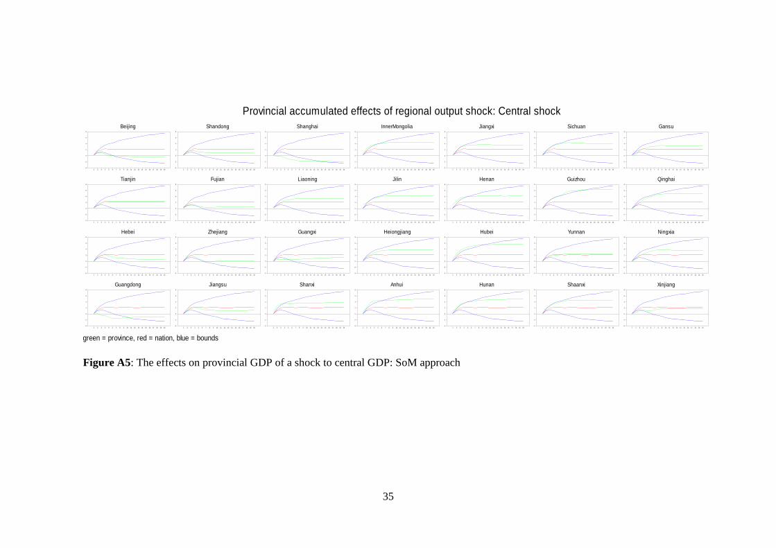
35
Figure A5: The effects on provincial GDP of a shock to central GDP: SoM approach
Provincial accumulated effects of regional output shock: Central shock
green = province, red = nation, blue = bounds
Beijing
1 2 3 4 5 6 7 8 9 10 11 12 13 14 15 16 17 18 19 20-4
-2
0
2
4
6
8
Tianjin
1 2 3 4 5 6 7 8 9 10 11 12 13 14 15 16 17 18 19 20-4
-2
0
2
4
6
8
Hebei
1 2 3 4 5 6 7 8 9 10 11 12 13 14 15 16 17 18 19 20-4
-2
0
2
4
6
8
Guangdong
1 2 3 4 5 6 7 8 9 10 11 12 13 14 15 16 17 18 19 20-4
-2
0
2
4
6
8
Shandong
1 2 3 4 5 6 7 8 9 10 11 12 13 14 15 16 17 18 19 20-4
-2
0
2
4
6
8
Fujian
1 2 3 4 5 6 7 8 9 10 11 12 13 14 15 16 17 18 19 20-4
-2
0
2
4
6
8
Zhejiang
1 2 3 4 5 6 7 8 9 10 11 12 13 14 15 16 17 18 19 20-4
-2
0
2
4
6
8
Jiangsu
1 2 3 4 5 6 7 8 9 10 11 12 13 14 15 16 17 18 19 20-4
-2
0
2
4
6
8
Shanghai
1 2 3 4 5 6 7 8 9 10 11 12 13 14 15 16 17 18 19 20-4
-2
0
2
4
6
8
Liaoning
1 2 3 4 5 6 7 8 9 10 11 12 13 14 15 16 17 18 19 20-4
-2
0
2
4
6
8
Guangxi
1 2 3 4 5 6 7 8 9 10 11 12 13 14 15 16 17 18 19 20-4
-2
0
2
4
6
8
Shanxi
1 2 3 4 5 6 7 8 9 10 11 12 13 14 15 16 17 18 19 20-4
-2
0
2
4
6
8
InnerMongolia
1 2 3 4 5 6 7 8 9 10 11 12 13 14 15 16 17 18 19 20-4
-2
0
2
4
6
8
Jilin
1 2 3 4 5 6 7 8 9 10 11 12 13 14 15 16 17 18 19 20-4
-2
0
2
4
6
8
Heiongjiang
1 2 3 4 5 6 7 8 9 10 11 12 13 14 15 16 17 18 19 20-4
-2
0
2
4
6
8
Anhui
1 2 3 4 5 6 7 8 9 10 11 12 13 14 15 16 17 18 19 20-4
-2
0
2
4
6
8
Jiangxi
1 2 3 4 5 6 7 8 9 10 11 12 13 14 15 16 17 18 19 20-4
-2
0
2
4
6
8
Henan
1 2 3 4 5 6 7 8 9 10 11 12 13 14 15 16 17 18 19 20-4
-2
0
2
4
6
8
Hubei
1 2 3 4 5 6 7 8 9 10 11 12 13 14 15 16 17 18 19 20-4
-2
0
2
4
6
8
Hunan
1 2 3 4 5 6 7 8 9 10 11 12 13 14 15 16 17 18 19 20-4
-2
0
2
4
6
8
Sichuan
1 2 3 4 5 6 7 8 9 10 11 12 13 14 15 16 17 18 19 20-4
-2
0
2
4
6
8
Guizhou
1 2 3 4 5 6 7 8 9 10 11 12 13 14 15 16 17 18 19 20-4
-2
0
2
4
6
8
Yunnan
1 2 3 4 5 6 7 8 9 10 11 12 13 14 15 16 17 18 19 20-4
-2
0
2
4
6
8
Shaanxi
1 2 3 4 5 6 7 8 9 10 11 12 13 14 15 16 17 18 19 20-4
-2
0
2
4
6
8
Gansu
1 2 3 4 5 6 7 8 9 10 11 12 13 14 15 16 17 18 19 20-4
-2
0
2
4
6
8
Qinghai
1 2 3 4 5 6 7 8 9 10 11 12 13 14 15 16 17 18 19 20-4
-2
0
2
4
6
8
Ningxia
1 2 3 4 5 6 7 8 9 10 11 12 13 14 15 16 17 18 19 20-4
-2
0
2
4
6
8
Xinjiang
1 2 3 4 5 6 7 8 9 10 11 12 13 14 15 16 17 18 19 20-4
-2
0
2
4
6
8
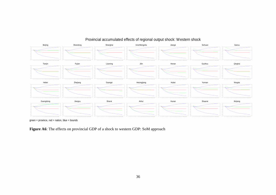
36
Figure A6: The effects on provincial GDP of a shock to western GDP: SoM approach
Provincial accumulated effects of regional output shock: Western shock
green = province, red = nation, blue = bounds
Beijing
1 2 3 4 5 6 7 8 9 10 11 12 13 14 15 16 17 18 19 20-6
-5
-4
-3
-2
-1
0
1
2
Tianjin
1 2 3 4 5 6 7 8 9 10 11 12 13 14 15 16 17 18 19 20-6
-5
-4
-3
-2
-1
0
1
2
Hebei
1 2 3 4 5 6 7 8 9 10 11 12 13 14 15 16 17 18 19 20-6
-5
-4
-3
-2
-1
0
1
2
Guangdong
1 2 3 4 5 6 7 8 9 10 11 12 13 14 15 16 17 18 19 20-6
-5
-4
-3
-2
-1
0
1
2
Shandong
1 2 3 4 5 6 7 8 9 10 11 12 13 14 15 16 17 18 19 20-6
-5
-4
-3
-2
-1
0
1
2
Fujian
1 2 3 4 5 6 7 8 9 10 11 12 13 14 15 16 17 18 19 20-6
-5
-4
-3
-2
-1
0
1
2
Zhejiang
1 2 3 4 5 6 7 8 9 10 11 12 13 14 15 16 17 18 19 20-6
-5
-4
-3
-2
-1
0
1
2
Jiangsu
1 2 3 4 5 6 7 8 9 10 11 12 13 14 15 16 17 18 19 20-6
-5
-4
-3
-2
-1
0
1
2
Shanghai
1 2 3 4 5 6 7 8 9 10 11 12 13 14 15 16 17 18 19 20-6
-5
-4
-3
-2
-1
0
1
2
Liaoning
1 2 3 4 5 6 7 8 9 10 11 12 13 14 15 16 17 18 19 20-6
-5
-4
-3
-2
-1
0
1
2
Guangxi
1 2 3 4 5 6 7 8 9 10 11 12 13 14 15 16 17 18 19 20-6
-5
-4
-3
-2
-1
0
1
2
Shanxi
1 2 3 4 5 6 7 8 9 10 11 12 13 14 15 16 17 18 19 20-6
-5
-4
-3
-2
-1
0
1
2
InnerMongolia
1 2 3 4 5 6 7 8 9 10 11 12 13 14 15 16 17 18 19 20-6
-5
-4
-3
-2
-1
0
1
2
Jilin
1 2 3 4 5 6 7 8 9 10 11 12 13 14 15 16 17 18 19 20-6
-5
-4
-3
-2
-1
0
1
2
Heiongjiang
1 2 3 4 5 6 7 8 9 10 11 12 13 14 15 16 17 18 19 20-6
-5
-4
-3
-2
-1
0
1
2
Anhui
1 2 3 4 5 6 7 8 9 10 11 12 13 14 15 16 17 18 19 20-6
-5
-4
-3
-2
-1
0
1
2
Jiangxi
1 2 3 4 5 6 7 8 9 10 11 12 13 14 15 16 17 18 19 20-6
-5
-4
-3
-2
-1
0
1
2
Henan
1 2 3 4 5 6 7 8 9 10 11 12 13 14 15 16 17 18 19 20-6
-5
-4
-3
-2
-1
0
1
2
Hubei
1 2 3 4 5 6 7 8 9 10 11 12 13 14 15 16 17 18 19 20-6
-5
-4
-3
-2
-1
0
1
2
Hunan
1 2 3 4 5 6 7 8 9 10 11 12 13 14 15 16 17 18 19 20-6
-5
-4
-3
-2
-1
0
1
2
Sichuan
1 2 3 4 5 6 7 8 9 10 11 12 13 14 15 16 17 18 19 20-6
-5
-4
-3
-2
-1
0
1
2
Guizhou
1 2 3 4 5 6 7 8 9 10 11 12 13 14 15 16 17 18 19 20-6
-5
-4
-3
-2
-1
0
1
2
Yunnan
1 2 3 4 5 6 7 8 9 10 11 12 13 14 15 16 17 18 19 20-6
-5
-4
-3
-2
-1
0
1
2
Shaanxi
1 2 3 4 5 6 7 8 9 10 11 12 13 14 15 16 17 18 19 20-6
-5
-4
-3
-2
-1
0
1
2
Gansu
1 2 3 4 5 6 7 8 9 10 11 12 13 14 15 16 17 18 19 20-6
-5
-4
-3
-2
-1
0
1
2
Qinghai
1 2 3 4 5 6 7 8 9 10 11 12 13 14 15 16 17 18 19 20-6
-5
-4
-3
-2
-1
0
1
2
Ningxia
1 2 3 4 5 6 7 8 9 10 11 12 13 14 15 16 17 18 19 20-6
-5
-4
-3
-2
-1
0
1
2
Xinjiang
1 2 3 4 5 6 7 8 9 10 11 12 13 14 15 16 17 18 19 20-6
-5
-4
-3
-2
-1
0
1
2
37
Editor, UWA Economics Discussion Papers: Sam Hak Kan Tang University of Western Australia 35 Sterling Hwy Crawley WA 6009 Australia Email: [email protected] The Economics Discussion Papers are available at: 1980 – 2002: http://ecompapers.biz.uwa.edu.au/paper/PDF%20of%20Discussion%20Papers/ Since 2001: http://ideas.repec.org/s/uwa/wpaper1.html Since 2004: http://www.business.uwa.edu.au/school/disciplines/economics
ECONOMICS DISCUSSION PAPERS 2015
DP NUMBER
AUTHORS TITLE
15.01 Robertson, P.E. and Robitaille, M.C. THE GRAVITY OF RESOURCES AND THE TYRANNY OF DISTANCE
15.02 Tyers, R. FINANCIAL INTEGRATION AND CHINA’S GLOBAL IMPACT
15.03 Clements, K.W. and Si, J. MORE ON THE PRICE-RESPONSIVENESS OF FOOD CONSUMPTION
15.04 Tang, S.H.K. PARENTS, MIGRANT DOMESTIC WORKERS, AND CHILDREN’S SPEAKING OF A SECOND LANGUAGE: EVIDENCE FROM HONG KONG
15.05 Tyers, R. CHINA AND GLOBAL MACROECONOMIC INTERDEPENDENCE
15.06 Fan, J., Wu, Y., Guo, X., Zhao, D. and Marinova, D.
REGIONAL DISPARITY OF EMBEDDED CARBON FOOTPRINT AND ITS SOURCES IN CHINA: A CONSUMPTION PERSPECTIVE
15.07 Fan, J., Wang, S., Wu, Y., Li, J. and Zhao, D.
BUFFER EFFECT AND PRICE EFFECT OF A PERSONAL CARBON TRADING SCHEME
15.08 Neill, K. WESTERN AUSTRALIA’S DOMESTIC GAS RESERVATION POLICY THE ELEMENTAL ECONOMICS
15.09 Collins, J., Baer, B. and Weber, E.J. THE EVOLUTIONARY FOUNDATIONS OF ECONOMICS
15.10 Siddique, A., Selvanathan, E. A. and Selvanathan, S.
THE IMPACT OF EXTERNAL DEBT ON ECONOMIC GROWTH: EMPIRICAL EVIDENCE FROM HIGHLY INDEBTED POOR COUNTRIES
15.11 Wu, Y. LOCAL GOVERNMENT DEBT AND ECONOMIC GROWTH IN CHINA
15.12 Tyers, R. and Bain, I. THE GLOBAL ECONOMIC IMPLICATIONS OF FREER SKILLED MIGRATION
15.13 Chen, A. and Groenewold, N. AN INCREASE IN THE RETIREMENT AGE IN CHINA: THE REGIONAL ECONOMIC EFFECTS
15.14 Knight, K. PIGOU, A LOYAL MARSHALLIAN?

38
15.15 Kristoffersen, I. THE AGE-HAPPINESS PUZZLE: THE ROLE OF ECONOMIC CIRCUMSTANCES AND FINANCIAL SATISFACTION
15.16 Azwar, P. and Tyers, R. INDONESIAN MACRO POLICY THROUGH TWO CRISES
15.17 Asano, A. and Tyers, R. THIRD ARROW REFORMS AND JAPAN’S ECONOMIC PERFORMANCE
15.18 Arthmar, R. and McLure, M. ON BRITAIN’S RETURN TO THE GOLD STANDARD: WAS THERE A ‘PIGOU-MCKENNA SCHOOL’?
15.19 Fan, J., Li, Y., Wu, Y., Wang, S., and Zhao, D.
ALLOWANCE TRADING AND ENERGY CONSUMPTION UNDER A PERSONAL CARBON TRADING SCHEME: A DYNAMIC PROGRAMMING APPROACH
15.20 Shehabi, M. AN EXTRAORDINARY RECOVERY: KUWAIT FOLLOWING THE GULF WAR
15.21 Siddique, A., Sen, R., and Srivastava, S.
AUSTRALIA-THAILAND TRADE: AN ANALYSIS OF COMPETITIVENESS AND THE EFFECTS OF THE BILATERAL FTA
15.22 Tyers, R. SLOWER GROWTH AND VULNERABILITY TO RECESSION: UPDATING CHINA’S GLOBAL IMPACT
15.23 Arthmar, R. and McLure, M. PIGOU ON WAR FINANCE AND STATE ACTION
15.24 Wu, Y. CHINA'S CAPITAL STOCK SERIES BY REGION AND SECTOR
15.25 Clements, K. and Si, J. ENGEL'S LAW, DIET DIVERSITY AND THE QUALITY OF FOOD CONSUMPTION
15.26 Chen, S. SHIFTS OF DISTORTION AND CORRUPTION OVER LOCAL POLITICAL CYCLES IN CHINA
15.27 Chen, S. THE EFFECT OF A FISCAL SQUEEZE ON TAX NFORCEMENT: EVIDENCE FROM A NATURAL EXPERIMENT IN CHINA
15.28 Jetter, M. BLOWING THINGS UP: THE EFFECT OF MEDIA ATTENTION ON TERRORISM
15.29 Tang, S. MEDIUM-TERM MACROECONOMIC VOLATILITY AND ECONOMIC DEVELOPMENT: A NEW TECHNIQUE
15.30 Alim, A., Hartley, P. and Lan, Y. ASIAN SPOT PRICES FOR LNG OTHER ENERGY COMMODITIES
15.31 Gannon, B., Harris, D., Harris, M., Magnusson, L., Hollingsworth, B., Inder, B., Maitra, P, and Munford, L.
NEW APPROACHES TO ESTIMATING THE CHILD HEALTH-PARENTAL INCOME RELATIONSHIP
15.32 Czaika, M. and Parsons, C. THE GRAVITY OF HIGH SKILLED MIGRATION POLICIES
15.33 Parsons, C., Rojon, S., Samanani, F, and Wettach, L.
CONCEPTUALISING INTERNATIONAL HIGH-SKILLED MIGRATION
15.34 Chen, S. VAT RATE DISPERSION AND TFP LOSS IN CHINA’S MANUFACTURING SECTOR
15.35 Tait, L., Siddique, A. and Chatterjee, I. FOREIGN AID AND ECONOMIC GROWTH IN SUB-SAHARAN AFRICA

39
ECONOMICS DISCUSSION PAPERS 2016
DP NUMBER
AUTHORS TITLE
16.01 Xu, R., Wu, Y. and Luan, J. ANALYSIS OF FARMERS’ WILLINGNESS TO ADOPT GENETICALLY MODIFIED INSECT-RESISTANT RICE IN CHINA
16.02 Lia, Y., Fan, J., Zhao, D., Wu, Y. and Li, J.
TIERED GASOLINE PRICING: A PERSONAL CARBON TRADING PERSPECTIVE
16.03 Clements, K.W., Lan, Y. and Si, J. UNCERTAINTY IN CURRENCY MISPRICING
16.04 Parsons, C. and Vézina, P.L. MIGRANT NETWORKS AND TRADE:THE VIETNAMESE BOAT PEOPLE AS A NATURAL EXPERIMENT
16.05 Chang, S., Connelly, R. and Ma, P.
WHAT WILL YOU DO IF I SAY ‘I DO’?: THE EFFECT OF THE SEX RATIO ON TIME USE WITHIN TAIWANESE MARRIED COUPLES
16.06 Yu, F. and Wu, Y. BIASES IN PATENT EXAMINATION AND FIRMS’ RESPONSES: EVIDENCE FROM THE PHARMACEUTICAL INDUSTRY
16.07 Fan, J., Li, J., Wu, Y., Wang, S. and Zhao, D.
THE EFFECTS OF ALLOWANCE PRICE ON ENERGY DEMAND UNDER A PERSONAL CARBON TRADING SCHEME
16.08 Golley, J., Tyers, R. and Zhou, Y. CONTRACTIONS IN CHINESE FERTILITY AND SAVINGS: LONG RUN DOMESTIC AND GLOBAL IMPLICATIONS
16.09 McGrath, G. and Neill, K. FOREIGN AND DOMESTIC OWNERSHIP IN WESTERN AUSTRALIA’S GAS MARKET
16.10 Clements, K.W. and Si, J. SIMPLIFYING THE BIG MAC INDEX
16.11 Priyati, R.Y. and Tyers, R. PRICE RELATIONSHIPS IN VEGETABLE OIL AND ENERGY MARKETS
16.12 Wu, J., Wu, Y. and Wang, B. THE GREENNESS OF CHINESE CITIES: CARBON DIOXIDE EMISSION AND ITS DETERMINANTS
16.13 Arslan, C., Dumont, J.C., Kone, Z., Özden, Ç., Parsons, C. and Xenogiani, T.
INTERNATIONAL MIGRATION TO THE OECD IN THE TWENTY-FIRST CENTURY
16.14 Tomioka, K. and Tyers, R. HAS FOREIGN GROWTH CONTRIBUTED TO STAGNATION AND INEQUALITY IN JAPAN?
16.15 Donovan, J. and Hartley, P. RIDING THE IRON ORE CYCLE: ACTIONS OF AUSTRALIA’S MAJOR PRODUCERS
16.16 Czaika, M. and Parsons, C. HIGH-SKILLED MIGRATION IN TIMES OF GLOBAL ECONOMIC CRISIS
16.17 Lefroy, T., Key, J. and Kingwell, R. A LONGITUDINAL EXAMINATION OF BROADACRE FARM SIZE AND PERFORMANCE IN WESTERN AUSTRALIA
16.18 Arthmar, R. and McLure, M. SRAFFA, MYRDAL AND THE 1961 SÖDERSTRÖM GOLD MEDAL
19.19 Azwar, P. and Tyers, R. POST-GFC EXTERNAL SHOCKS AND INDONESIAN ECONOMIC PERFORMANCE
19.20 Chen, A. and Groenewold, N. OUTPUT SHOCKS IN CHINA: DO THE DISTRIBUTIONAL EFFECTS DEPEND ON THE REGIONAL SOURCE?