Policy Research Working Paper 6750

Economic Growth in Ghana

Determinants and Prospect

Anna K. Raggl

The World BankAfrica RegionPoverty Reduction and Economic Management DepartmentJanuary 2014

WPS6750P

ublic

Dis

clos

ure

Aut

horiz

edP

ublic

Dis

clos

ure

Aut

horiz

edP

ublic

Dis

clos

ure

Aut

horiz

edP

ublic

Dis

clos

ure

Aut

horiz

edP

ublic

Dis

clos

ure

Aut

horiz

edP

ublic

Dis

clos

ure

Aut

horiz

edP

ublic

Dis

clos

ure

Aut

horiz

edP

ublic

Dis

clos

ure

Aut

horiz

ed

Produced by the Research Support Team

Abstract

The Policy Research Working Paper Series disseminates the findings of work in progress to encourage the exchange of ideas about development issues. An objective of the series is to get the findings out quickly, even if the presentations are less than fully polished. The papers carry the names of the authors and should be cited accordingly. The findings, interpretations, and conclusions expressed in this paper are entirely those of the authors. They do not necessarily represent the views of the International Bank for Reconstruction and Development/World Bank and its affiliated organizations, or those of the Executive Directors of the World Bank or the governments they represent.

Policy Research Working Paper 6750

This paper employs a simple cross-country panel framework to assess the determinants of growth in Ghana’s gross domestic product over the past four decades. A set of standard covariates is used to explain growth rates. Natural resource variables are included because the effects of natural resource rents in gross domestic products are of particular interest for Ghana. Using the preferred specification, Ghana’s growth potential is predicted for the upcoming decades under different scenarios. The results indicate that under the most pessimistic scenario of no improvements in the

This paper is a product of the Poverty Reduction and Economic Management Department, Africa Region. It is part of a larger effort by the World Bank to provide open access to its research and make a contribution to development policy discussions around the world. Policy Research Working Papers are also posted on the Web at http://econ.worldbank.org. The author may be contacted at Anna.Raggl@wu.ac.at.

determinants of growth compared with the period 2005-09, Ghana’s gross domestic product per capita growth rates will stagnate at approximately 4.5 percent during the next decade and decrease thereafter. If the policy measures and country characteristics improve in the way they did in the past three decades, average per capita growth rates of roughly 5.5 percent could be reached during 2015–34. Taking into account the expected oil production until 2034 adds 0.6 percentage points to projected gross domestic product growth rates on average.

Economic Growth in Ghana: Determinants and Prospects∗

Anna K. Raggl†

Keywords: Economic growth, natural resources, oil production, panel growth models, Ghana,

Sub-Saharan Africa.

JEL Classification Codes: O11, O13, O55, Q43

Sector Board Code: EPOL

∗This report serves as a background study for the World Bank’s Policy Note on Long Run Growth in Ghana(2014)†WiC - Wittgenstein Centre for Demography and Global Human Capital, WU - Vienna University of Economics

and Business. Address: Welthandelsplatz 1, 1020 Vienna, Austria. Email: anna.raggl@wu.ac.at. The authorgratefully acknowledges valuable contributions from Jesus Crespo Cuaresma, Leonardo Garrido, Santiago Herreraand Mathias Moser.

1 Introduction

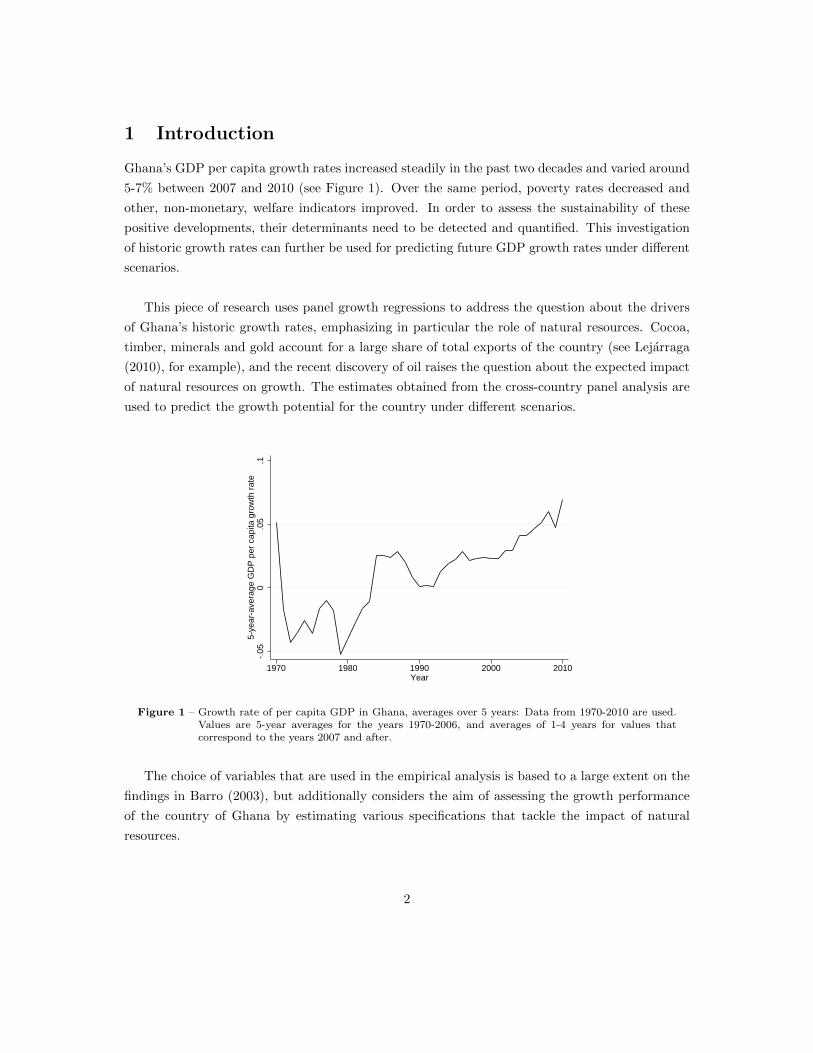
Ghana’s GDP per capita growth rates increased steadily in the past two decades and varied around

5-7% between 2007 and 2010 (see Figure 1). Over the same period, poverty rates decreased and

other, non-monetary, welfare indicators improved. In order to assess the sustainability of these

positive developments, their determinants need to be detected and quantified. This investigation

of historic growth rates can further be used for predicting future GDP growth rates under different

scenarios.

This piece of research uses panel growth regressions to address the question about the drivers

of Ghana’s historic growth rates, emphasizing in particular the role of natural resources. Cocoa,

timber, minerals and gold account for a large share of total exports of the country (see Lejarraga

(2010), for example), and the recent discovery of oil raises the question about the expected impact

of natural resources on growth. The estimates obtained from the cross-country panel analysis are

used to predict the growth potential for the country under different scenarios.

-.05

0.0

5.1

5-ye

ar-a

vera

ge G

DP

per

cap

ita g

row

th r

ate

1970 1980 1990 2000 2010Year

Figure 1 – Growth rate of per capita GDP in Ghana, averages over 5 years: Data from 1970-2010 are used.Values are 5-year averages for the years 1970-2006, and averages of 1-4 years for values thatcorrespond to the years 2007 and after.

The choice of variables that are used in the empirical analysis is based to a large extent on the

findings in Barro (2003), but additionally considers the aim of assessing the growth performance

of the country of Ghana by estimating various specifications that tackle the impact of natural

resources.

2

The dataset covers the period 1970-2009 and contains economic, political and institutional

characteristics of 151 countries, thereby extending the analysis in Barro (2003) by roughly 15 years

and 80 countries. We estimate different specifications of growth regressions controlling for fixed

country and period effects, trying to explain a large share of within-country variations in growth

rates.

The findings suggest that education significantly increases GDP per capita growth rates, an

effect that is larger in countries with a relatively low initial GDP per capita. Furthermore, invest-

ment, openness to trade as well as natural resources are found to be robust determinants of income

growth, all related positively to growth. Government consumption seems to decrease GDP growth

rates in the long run. Relating institutional characteristics of countries to the estimated country-

specific fixed effects shows that there exists a strong positive correlation between them. Although

no causal interpretations can be made in this context, the finding supports the supposition that

fixed effects capture the persistent part of the institutional environment and an improvement of

the quality of institutions is favorable for a country and translates into higher GDP per capita

growth.

Based on the performed growth regressions, we predict Ghana’s future growth potential for

different scenarios. In a baseline scenario, where investment, natural resources, government expen-

ditures and other covariates are assumed to remain at the level of 2005-09, we find that average

growth rates are slightly above 4% in the upcoming two decades. In a more favorable scenario,

where it is assumed that the covariates behave as they did since the 1980s, predicted growth rates

increase by about 1%-point as compared to the baseline scenario. Finally, when taking into account

the expected oil production in Ghana, GDP growth is likely to reach 6.2-6.5% in the next 15-20

years.

The paper is organized as follows. Before the results are discussed in Section 5, the model

specification is described in Section 2 and the econometric methodology and the data are described

in Sections 3 and 4. Section 6 applies the results to predict GDP per capita growth rates for Ghana

until 2030 and Section 7 summarizes and concludes.

2 Model Specification

The specifications of the growth regressions are based on the findings in Barro (2003), and aug-

mented by variables that are of particular interest for Ghana.

The dependent variable is the arithmetic average of the real GDP per capita growth rate of a

country over each 5-year period during 1970-2009. The basic specification includes country fixed

3

effects and time dummy variables and a set of variables that is explained in the following. In order

to control for (conditional) convergence effects, the (natural logarithm of the) level of GDP per

capita at the beginning of each 5-year period is included in the regression. The parameter estimate

associated with this variable is expected to be negative, as relatively low levels of GDP per capita

increase growth rates (holding all other factors constant). Its magnitude can be interpreted as the

speed of (conditional) convergence to a country-specific equilibrium growth rate. Human capital

enters as the share of the (female and male) working age population with tertiary education. In

order to alleviate a potential endogeneity bias due to simultaneity, the value at the start of each

period is used.

A further set of basic covariates are policy related variables and national characteristics. A vari-

able for international openness, measured as imports plus exports as shares of GDP, is included

to assess the effects of trade and globalization. As trade shares are highly correlated with country

sizes, Barro (2003) suggests adjusting the openness measure for this relation. More specifically, the

openness variable is regressed on the logarithms of the population and area (in square-kilometers)

of the countries, and only the remaining part of the measure is used in the growth regression. The

adjusted openness to trade of the countries enters each regression as an average over the 5-year

periods for each country. Additionally, 5-year averages of inflation, government consumption1 and

investment, the latter two as shares in total GDP, are added to the basic regression model. Finally,

as a proxy for institutional quality, a democracy index is included.

The oil production expected in Ghana during the upcoming decades and the country’s depen-

dency on cocoa, timber, gold and minerals raise the question about the growth effects of natural

resources in general, and oil production in particular. We address this issue by including different

variations of natural resource variables in the panel growth regressions. First, the 5-year averages of

natural resource rents as shares of GDP are used as a regressor. This variable combines rents from

oil, natural gas, coal, minerals and forest. As this variable does not allow to isolate an effect of oil

production per se, the measure is split into rents obtained from oil production and non-oil natural

resource rents in a subsequent specification. The coefficient of the variable that measures oil rents

as shares in GDP might still hide some heterogeneities. For that reason we further decompose the

variable by interacting the oil rents with dummy variables indicating the relative importance of oil

production as compared to other economies. This allows the effects of oil rents on GDP growth to

differ across countries with varying oil intensities. The results of this final specification are used

to perform in- and out-of-sample predictions of Ghana’s growth rates.

1Barro (2003) suggests subtracting expenditures for defense and education from government consumption, asthese should be considered as investments. Data limitations do not allow us to perform a similar adjustment.

4

The data sources of the variables described above can be found in Section 4, and Table 1 briefly

summarizes the variables and their respective sources.

In the context of economic growth and especially in interaction with the role of natural resources,

it would be of particular interest to study the impact of the quality of institutions of the countries.

Most institutional indicators, such as those proxying the rule of law, government effectiveness or

political stability, are not available for a sufficient number of countries and years to include them

in the growth regressions. Additionally, institutional characteristics are very persistent, which

complicates the identification of the parameters in a fixed effects framework. To the extent that

institutional variables are constant over the period 1970-2009, they are captured by the fixed

country effects and only significant yearly deviations from the long-run country means would allow

including them in the estimation. The advantage of the persistent nature of institutions is that fixed

country effects control for general differences in the quality of institutions across countries, even

when the indicators are not available for most of the years considered. This approach, however,

does not allow us to isolate the effect of institutions on GDP growth, but the risk for a potential

omitted variable bias is reduced. In an extension of the analysis below, we assess the correlation of

the estimated fixed effects and a number of institutional quality indicators (measured in a recent

year, to maximize the sample for the analysis) in an attempt to explain parts of the variation of

fixed effects across countries.

3 Econometric Methodology

We estimate the specifications discussed above controlling for fixed country effects and including

period dummy variables. The period dummies control for effects that are specific for a certain

period and have an impact on all countries in a given period. The country specific fixed effects

allow controlling for unobserved heterogeneity as they capture effects that are characteristic for a

country and that do not vary over time, such as most geographical factors, colonial linkages, or

cultural factors inherent to a country. The conclusions we can draw from this analysis are within-

country effects, and do not reflect between country effects.

In particular, we estimate a model of the following form

yit = α+

K∑k=1

βkxkit + µi + δt + εit (1)

where yit is the GDP per capita growth rate of country i in year t, α is a constant, xit are

the K explanatory variables corresponding to country i and period t, µi are country-specific fixed

effects, δt are time fixed effects and εit is an error term.

5

The explanatory variables vary by specification, but time and country fixed effects are in-

cluded in every specification, so are the log of the initial GDP, education, investment, government

consumption, inflation, democracy, trade openness and some measure of natural resource rents.

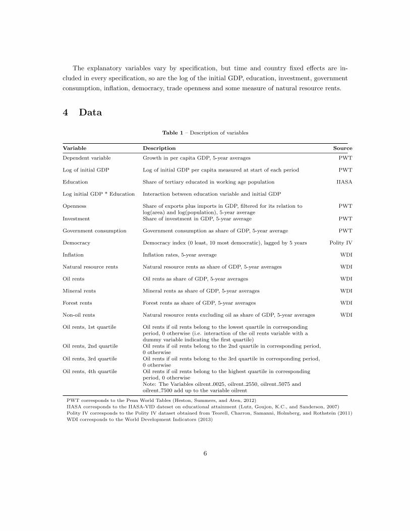
4 Data

Table 1 – Description of variables

Variable Description Source

Dependent variable Growth in per capita GDP, 5-year averages PWT

Log of initial GDP Log of initial GDP per capita measured at start of each period PWT

Education Share of tertiary educated in working age population IIASA

Log initial GDP * Education Interaction between education variable and initial GDP

Openness Share of exports plus imports in GDP, filtered for its relation tolog(area) and log(population), 5-year average

PWT

Investment Share of investment in GDP, 5-year average PWT

Government consumption Government consumption as share of GDP, 5-year average PWT

Democracy Democracy index (0 least, 10 most democratic), lagged by 5 years Polity IV

Inflation Inflation rates, 5-year average WDI

Natural resource rents Natural resource rents as share of GDP, 5-year averages WDI

Oil rents Oil rents as share of GDP, 5-year averages WDI

Mineral rents Mineral rents as share of GDP, 5-year averages WDI

Forest rents Forest rents as share of GDP, 5-year averages WDI

Non-oil rents Natural resource rents excluding oil as share of GDP, 5-year averages WDI

Oil rents, 1st quartile Oil rents if oil rents belong to the lowest quartile in correspondingperiod, 0 otherwise (i.e. interaction of the oil rents variable with adummy variable indicating the first quartile)

Oil rents, 2nd quartile Oil rents if oil rents belong to the 2nd quartile in corresponding period,0 otherwise

Oil rents, 3rd quartile Oil rents if oil rents belong to the 3rd quartile in corresponding period,0 otherwise

Oil rents, 4th quartile Oil rents if oil rents belong to the highest quartile in correspondingperiod, 0 otherwiseNote: The Variables oilrent 0025, oilrent 2550, oilrent 5075 andoilrent 7500 add up to the variable oilrent

PWT corresponds to the Penn World Tables (Heston, Summers, and Aten, 2012)

IIASA corresponds to the IIASA-VID dateset on educational attainment (Lutz, Goujon, K.C., and Sanderson, 2007)

Polity IV corresponds to the Polity IV dataset obtained from Teorell, Charron, Samanni, Holmberg, and Rothstein (2011)

WDI corresponds to the World Development Indicators (2013)

6

We use a dataset of 117-151 countries spanning the period 1970-2009. The four decades are

split into 8 time periods, each covering a 5-year window. Data availability does not allow to observe

each country in each period, the resulting database has the structure of an unbalanced panel and

the numbers of countries considered depends of the empirical specification. Most of the variables

enter as averages over the 5 years or initial values measured at the start of each period are used. Ta-

ble A.11 in the Appendix provides an overview of the countries and periods included in the analyses.

The dataset combines data from various sources. Per capita GDP (PPP converted, at constant

2005 prices) is taken from the Penn World Table (PWT) Version 7.1 (Heston, Summers, and Aten,

2012). Growth rates of per capita GDP are computed as log-differences of that variable. The value

of the logarithm of GDP per capita at the start of each period is used as a right hand side variable.

Government consumption, investment as well as the measure for openness and inflation are ob-

tained from the same source. Data on educational attainment are taken from an updated version of

the IIASA/VID Dataset on Educational Attainment (Lutz, Goujon, K.C., and Sanderson, 2007).

To control for the level of democracy of a country, an index from the Quality of Government Stan-

dard Data collection (Teorell, Charron, Samanni, Holmberg, and Rothstein, 2011) is used, and in

order to extend the time coverage we additionally use data on democracy provided by Bollen (1990).

A summary and brief description of the variables used can be found in Table 1.

5 Results

Column 1 of Table 2 shows the first baseline regression including the initial GDP per capita, hu-

man capital as well as an index for democracy, the openness ratio, government consumption and

investment as shares in GDP, inflation and 7 period dummies, where the first period (1970-74)

constitutes the reference category. The negative and significant coefficient of the lagged GDP

per capita variable indicates that countries with a relatively low initial income grow faster towards

their country specific equilibrium. The institutional variable, an index of democracy, does not show

significant effects in this specification. Likewise, education is not identified as a significant driver of

growth rates. This is a common problem in cross country growth regressions and often attributed

to differences in the quality of education across countries and over time (Hanushek and Wossmann,

2008), the lack of including the demographic structure of educational attainment (Lutz, Cuaresma,

and Sanderson, 2008), omitting (in)equality measures of schooling within a country (Sauer and Za-

gler, 2012) or heterogeneous effects across countries or over time. The specification in Column 1

assumes a linear relationship between education and growth and it does not allow the impact of

human capital to differ across countries. In the following, an interaction of the initial GDP per

7

capita and the education measure is included to address this issue.

Increases in government consumption lower growth rates (in long run perspective of this anal-

ysis), so do increases in inflation. Investment and the openness ratio of a country foster growth

significantly. These results are in line with Barro (2003).

As an addition to the set of variables suggested by Barro (2003), an aggregate measure of natural

resource rents is included in specification 1 and shows a positive impact of GDP growth rates of

the countries included. A disaggregation of this measure will shed further light on the impact of

natural resources on growth rates.

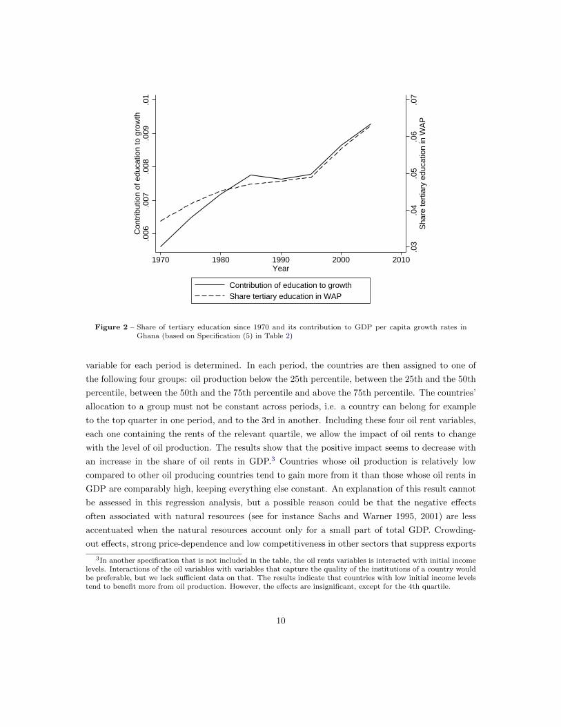
Additionally to the variables in Column 1, Column 2 of Table 2 includes an interaction of

education and the initial level of GDP. The findings show that the effect of human capital on

economic growth depends on the level of development of the country. The lower the initial income

level of a country, the higher the gains from a better educated working age population. For the

case of Ghana, the effects of the historic increases in education on per capita GDP growth rates are

plotted in Figure 22. The steady increase in the tertiary education of the working age population

between 1970 and 2009 contributes by roughly 0.5-0.9%-points to yearly GDP per capita growth

rates.

In the specifications 3-5 we are focusing on a decomposition of the natural capital variable.

The variable combines rents obtained from oil, natural gas, minerals, coal and forests. Splitting

the variable into rents from oil production and other natural capital rents (column 3 of Table 2)

suggests that while non-oil natural capital rents increase GDP growth, oil rents show no significant

impact on output growth. This however could be due to the heterogeneous nature of oil exporting

countries. While many countries obtain oil rents worth less than 1% of their GDP, some countries’

economy is more dependent on oil production and these might react to changes in oil rents in a

different way, an issue that is further addressed below.

Splitting the non-oil natural resource variable further into rents from minerals and forests (as

these two resources are of particular interest for Ghana), we find that minerals, as opposed to rents

from forests, increase GDP growth rates (Column 4). It should be noted, that the coefficients of

the other covariates do not change considerably when altering the natural resource variable.

Column 5 allows the impact of oil rents on GDP growth to depend on the relative size of the

oil rents in GDP. In order to implement that, the 25th, 50th and 75th percentile of the oil rent

2As specification 2 in Table 2 is not the preferred specification, the estimates shown in the figure are based onthe final specification in Column 5.

8

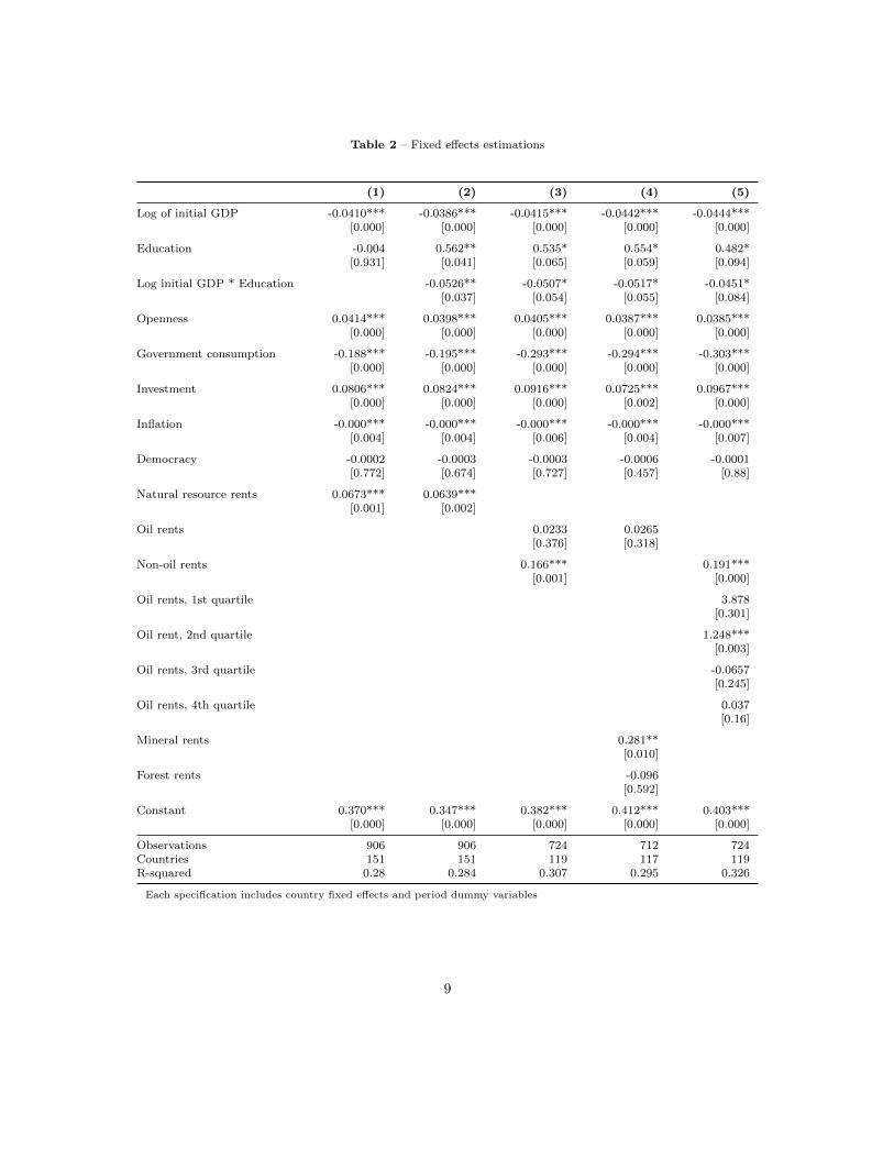
Table 2 – Fixed effects estimations

(1) (2) (3) (4) (5)

Log of initial GDP -0.0410*** -0.0386*** -0.0415*** -0.0442*** -0.0444***[0.000] [0.000] [0.000] [0.000] [0.000]

Education -0.004 0.562** 0.535* 0.554* 0.482*[0.931] [0.041] [0.065] [0.059] [0.094]

Log initial GDP * Education -0.0526** -0.0507* -0.0517* -0.0451*[0.037] [0.054] [0.055] [0.084]

Openness 0.0414*** 0.0398*** 0.0405*** 0.0387*** 0.0385***[0.000] [0.000] [0.000] [0.000] [0.000]

Government consumption -0.188*** -0.195*** -0.293*** -0.294*** -0.303***[0.000] [0.000] [0.000] [0.000] [0.000]

Investment 0.0806*** 0.0824*** 0.0916*** 0.0725*** 0.0967***[0.000] [0.000] [0.000] [0.002] [0.000]

Inflation -0.000*** -0.000*** -0.000*** -0.000*** -0.000***[0.004] [0.004] [0.006] [0.004] [0.007]

Democracy -0.0002 -0.0003 -0.0003 -0.0006 -0.0001[0.772] [0.674] [0.727] [0.457] [0.88]

Natural resource rents 0.0673*** 0.0639***[0.001] [0.002]

Oil rents 0.0233 0.0265[0.376] [0.318]

Non-oil rents 0.166*** 0.191***[0.001] [0.000]

Oil rents, 1st quartile 3.878[0.301]

Oil rent, 2nd quartile 1.248***[0.003]

Oil rents, 3rd quartile -0.0657[0.245]

Oil rents, 4th quartile 0.037[0.16]

Mineral rents 0.281**[0.010]

Forest rents -0.096[0.592]

Constant 0.370*** 0.347*** 0.382*** 0.412*** 0.403***[0.000] [0.000] [0.000] [0.000] [0.000]

Observations 906 906 724 712 724Countries 151 151 119 117 119R-squared 0.28 0.284 0.307 0.295 0.326

Each specification includes country fixed effects and period dummy variables

9

.03

.04

.05

.06

.07

Sha

re te

rtia

ry e

duca

tion

in W

AP

.006

.007

.008

.009

.01

Con

trib

utio

n of

edu

catio

n to

gro

wth

1970 1980 1990 2000 2010Year

Contribution of education to growthShare tertiary education in WAP

Figure 2 – Share of tertiary education since 1970 and its contribution to GDP per capita growth rates inGhana (based on Specification (5) in Table 2)

variable for each period is determined. In each period, the countries are then assigned to one of

the following four groups: oil production below the 25th percentile, between the 25th and the 50th

percentile, between the 50th and the 75th percentile and above the 75th percentile. The countries’

allocation to a group must not be constant across periods, i.e. a country can belong for example

to the top quarter in one period, and to the 3rd in another. Including these four oil rent variables,

each one containing the rents of the relevant quartile, we allow the impact of oil rents to change

with the level of oil production. The results show that the positive impact seems to decrease with

an increase in the share of oil rents in GDP.3 Countries whose oil production is relatively low

compared to other oil producing countries tend to gain more from it than those whose oil rents in

GDP are comparably high, keeping everything else constant. An explanation of this result cannot

be assessed in this regression analysis, but a possible reason could be that the negative effects

often associated with natural resources (see for instance Sachs and Warner 1995, 2001) are less

accentuated when the natural resources account only for a small part of total GDP. Crowding-

out effects, strong price-dependence and low competitiveness in other sectors that suppress exports

3In another specification that is not included in the table, the oil rents variables is interacted with initial incomelevels. Interactions of the oil variables with variables that capture the quality of the institutions of a country wouldbe preferable, but we lack sufficient data on that. The results indicate that countries with low initial income levelstend to benefit more from oil production. However, the effects are insignificant, except for the 4th quartile.

10

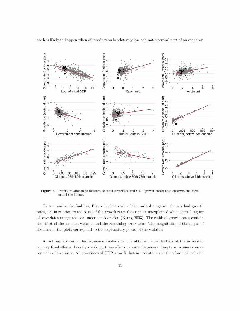
are less likely to happen when oil production is relatively low and not a central part of an economy.

-.35

-.3-

.25-

.2-.

15-.

1G

row

th r

ate

(res

idua

l par

t)

6 7 8 9 10 11Log of initial GDP

-.1

-.05

0.0

5.1

Gro

wth

rat

e (r

esid

ual p

art)

-1 0 1 2 3Openness

-.1

-.05

0.0

5.1

.15

Gro

wth

rat

e (r

esid

ual p

art)

0 .2 .4 .6 .8Investment

-.2

-.1

0.1

Gro

wth

rat

e (r

esid

ual p

art)

0 .2 .4 .6Government consumption

-.1

-.05

0.0

5.1

Gro

wth

rat

e (r

esid

ual p

art)

0 .1 .2 .3 .4Non-oil rents in GDP

-.05

0.0

5.1

.15

.2G

row

th r

ate

(res

idua

l par

t)

0 .001 .002 .003 .004Oil rents, below 25th quanitle

-.05

0.0

5.1

.15

Gro

wth

rat

e (r

esid

ual p

art)

0 .005 .01 .015 .02 .025Oil rents, 25th-50th quanitle

-.15

-.1

-.05

0.0

5G

row

th r

ate

(res

idua

l par

t)

0 .05 .1 .15 .2Oil rents, below 50th-75th quanitle

0.5

11.

5G

row

th r

ate

(res

idua

l par

t)

0 .2 .4 .6 .8 1Oil rents, above 75th quanitle

Figure 3 – Partial relationships between selected covariates and GDP growth rates; bold observations corre-spond the Ghana

To summarize the findings, Figure 3 plots each of the variables against the residual growth

rates, i.e. in relation to the parts of the growth rates that remain unexplained when controlling for

all covariates except the one under consideration (Barro, 2003). The residual growth rates contain

the effect of the omitted variable and the remaining error term. The magnitudes of the slopes of

the lines in the plots correspond to the explanatory power of the variable.

A last implication of the regression analysis can be obtained when looking at the estimated

country fixed effects. Loosely speaking, these effects capture the general long term economic envi-

ronment of a country. All covariates of GDP growth that are constant and therefore not included

11

in the regression, such as geographic factors, (constant) institutional characteristics, colonial link-

ages, climate, cultural conditions and similar, are summarized by the fixed effects. Technically,

the fixed effects would equal the growth rates in the case when all covariates, the constant and the

time fixed effects are zero. Factors that are common to all countries and common to all years are

summarized in the constant and the fixed effects show the country-specific deviations from that

constant. Thus, the mean of the fixed effects over all observations is zero.

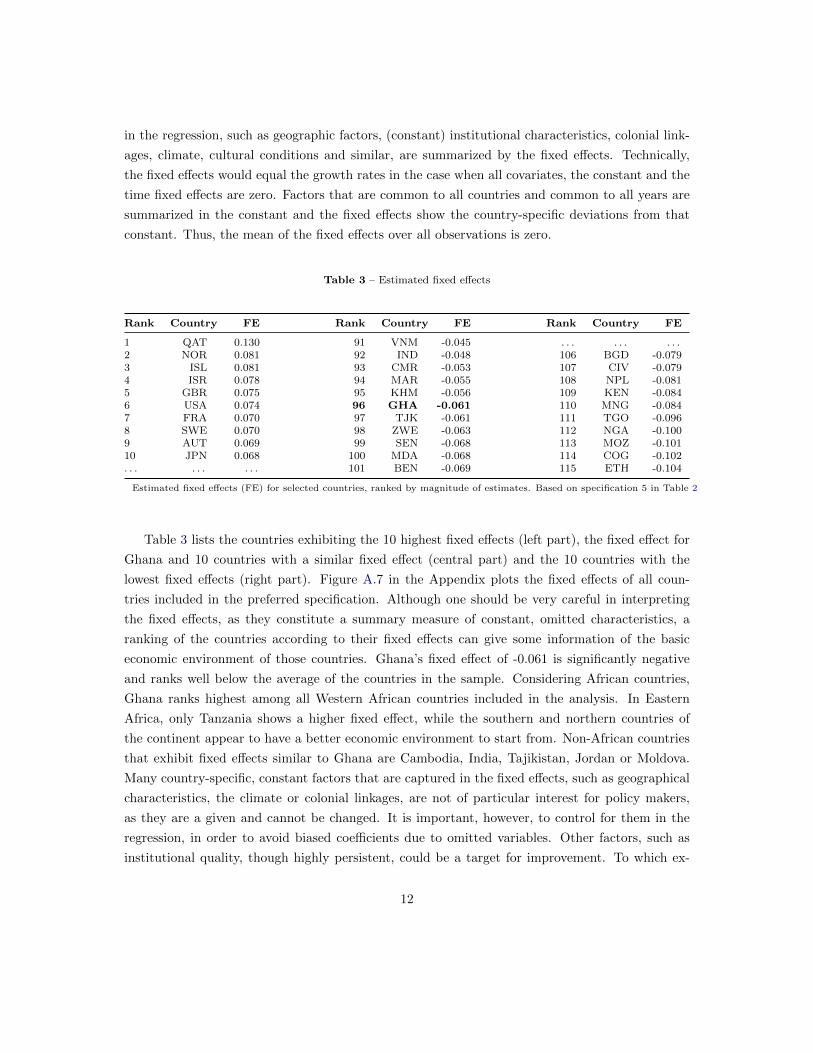
Table 3 – Estimated fixed effects

Rank Country FE Rank Country FE Rank Country FE

1 QAT 0.130 91 VNM -0.045 . . . . . . . . .2 NOR 0.081 92 IND -0.048 106 BGD -0.0793 ISL 0.081 93 CMR -0.053 107 CIV -0.0794 ISR 0.078 94 MAR -0.055 108 NPL -0.0815 GBR 0.075 95 KHM -0.056 109 KEN -0.0846 USA 0.074 96 GHA -0.061 110 MNG -0.0847 FRA 0.070 97 TJK -0.061 111 TGO -0.0968 SWE 0.070 98 ZWE -0.063 112 NGA -0.1009 AUT 0.069 99 SEN -0.068 113 MOZ -0.10110 JPN 0.068 100 MDA -0.068 114 COG -0.102. . . . . . . . . 101 BEN -0.069 115 ETH -0.104

Estimated fixed effects (FE) for selected countries, ranked by magnitude of estimates. Based on specification 5 in Table 2

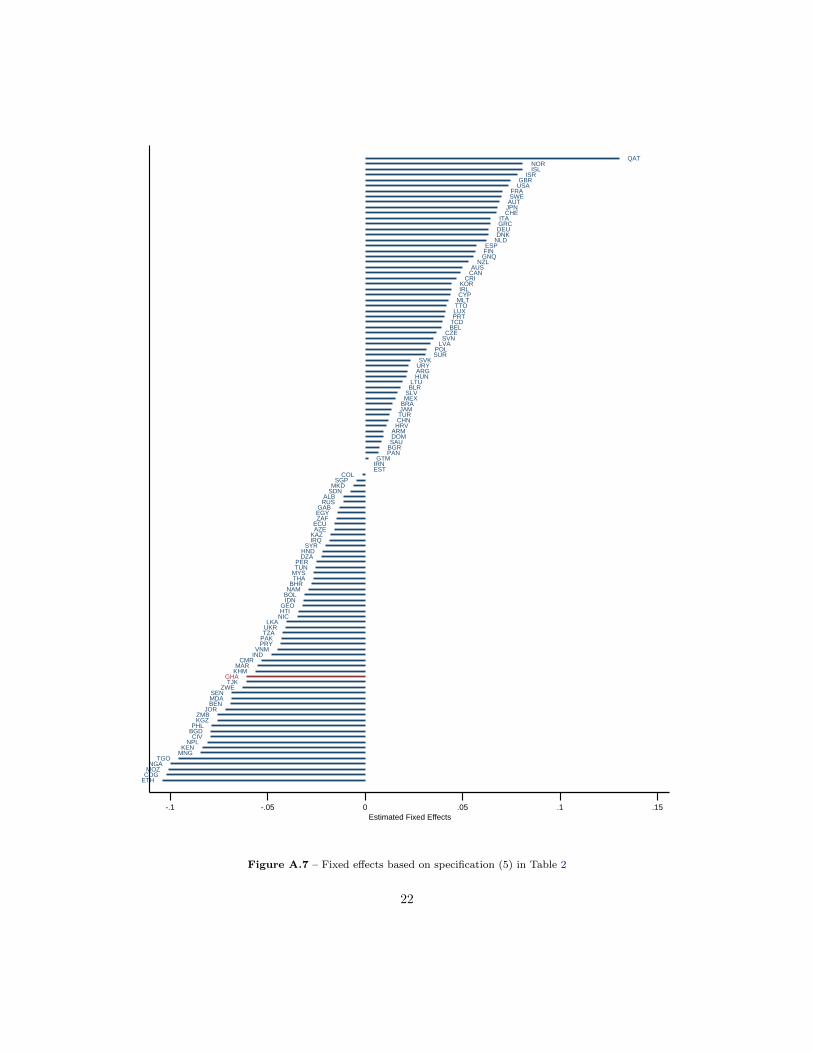
Table 3 lists the countries exhibiting the 10 highest fixed effects (left part), the fixed effect for

Ghana and 10 countries with a similar fixed effect (central part) and the 10 countries with the

lowest fixed effects (right part). Figure A.7 in the Appendix plots the fixed effects of all coun-

tries included in the preferred specification. Although one should be very careful in interpreting

the fixed effects, as they constitute a summary measure of constant, omitted characteristics, a

ranking of the countries according to their fixed effects can give some information of the basic

economic environment of those countries. Ghana’s fixed effect of -0.061 is significantly negative

and ranks well below the average of the countries in the sample. Considering African countries,

Ghana ranks highest among all Western African countries included in the analysis. In Eastern

Africa, only Tanzania shows a higher fixed effect, while the southern and northern countries of

the continent appear to have a better economic environment to start from. Non-African countries

that exhibit fixed effects similar to Ghana are Cambodia, India, Tajikistan, Jordan or Moldova.

Many country-specific, constant factors that are captured in the fixed effects, such as geographical

characteristics, the climate or colonial linkages, are not of particular interest for policy makers,

as they are a given and cannot be changed. It is important, however, to control for them in the

regression, in order to avoid biased coefficients due to omitted variables. Other factors, such as

institutional quality, though highly persistent, could be a target for improvement. To which ex-

12

tent the fixed effects reflect the institutional environment of a country cannot be assessed exactly,

but simple estimates of correlation coefficients show that fixed effects tend to be high whenever

institutional quality is relatively good, and vice versa. Table 4 displays the correlation between

the estimated country fixed effects and five selected indicators measuring the institutional quality.

All indicators are created in a way that an improvement of institutional quality materializes itself

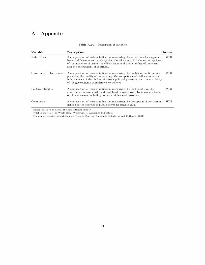
in a higher index. For a detailed description of the indicators, please refer to Table A.10 in the

Appendix. All off-diagonal elements in Columns 3-6 in Table 4 show the correlation between two

different indicators of institutional quality for the countries included in the regressions.

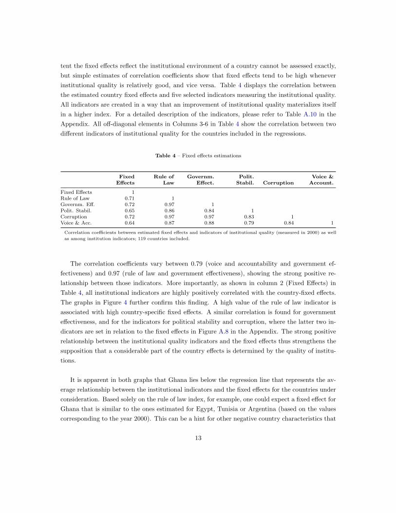
Table 4 – Fixed effects estimations

Fixed Rule of Governm. Polit. Voice &Effects Law Effect. Stabil. Corruption Account.

Fixed Effects 1Rule of Law 0.71 1Governm. Eff. 0.72 0.97 1Polit. Stabil. 0.65 0.86 0.84 1Corruption 0.72 0.97 0.97 0.83 1Voice & Acc. 0.64 0.87 0.88 0.79 0.84 1

Correlation coefficients between estimated fixed effects and indicators of institutional quality (measured in 2000) as well

as among institution indicators; 119 countries included.

The correlation coefficients vary between 0.79 (voice and accountability and government ef-

fectiveness) and 0.97 (rule of law and government effectiveness), showing the strong positive re-

lationship between those indicators. More importantly, as shown in column 2 (Fixed Effects) in

Table 4, all institutional indicators are highly positively correlated with the country-fixed effects.

The graphs in Figure 4 further confirm this finding. A high value of the rule of law indicator is

associated with high country-specific fixed effects. A similar correlation is found for government

effectiveness, and for the indicators for political stability and corruption, where the latter two in-

dicators are set in relation to the fixed effects in Figure A.8 in the Appendix. The strong positive

relationship between the institutional quality indicators and the fixed effects thus strengthens the

supposition that a considerable part of the country effects is determined by the quality of institu-

tions.

It is apparent in both graphs that Ghana lies below the regression line that represents the av-

erage relationship between the institutional indicators and the fixed effects for the countries under

consideration. Based solely on the rule of law index, for example, one could expect a fixed effect for

Ghana that is similar to the ones estimated for Egypt, Tunisia or Argentina (based on the values

corresponding to the year 2000). This can be a hint for other negative country characteristics that

13

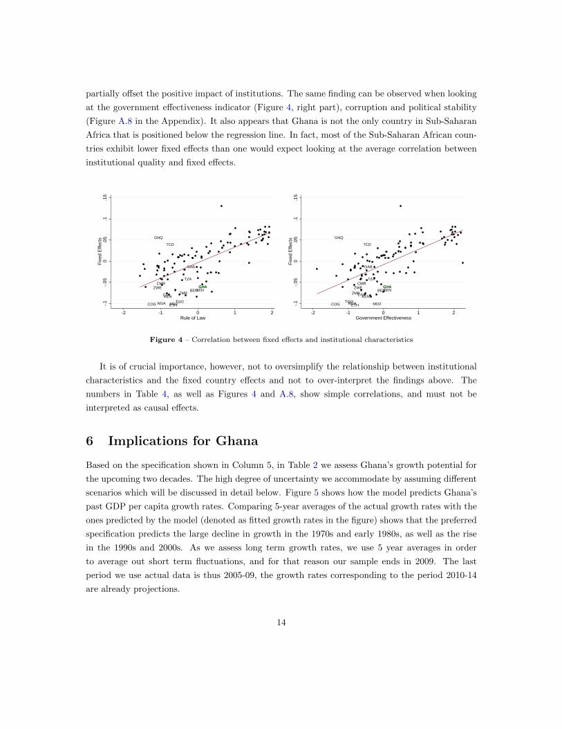
partially offset the positive impact of institutions. The same finding can be observed when looking

at the government effectiveness indicator (Figure 4, right part), corruption and political stability

(Figure A.8 in the Appendix). It also appears that Ghana is not the only country in Sub-Saharan

Africa that is positioned below the regression line. In fact, most of the Sub-Saharan African coun-

tries exhibit lower fixed effects than one would expect looking at the average correlation between

institutional quality and fixed effects.

CMR

MOZTGO

ETH

KEN

COG NGA

BEN

TZA

GHA

GNQ

GAB

ZMBZWE

SENCIV

TCD

GHA

-.1

-.05

0.0

5.1

.15

Fix

ed E

ffect

s

-2 -1 0 1 2Rule of Law

CMR

MOZTGO

ETH

KEN

COG NGA

BEN

TZA

GHA

GNQ

GAB

ZMBZWE

SENCIV

TCD

GHA

-.1

-.05

0.0

5.1

.15

Fix

ed E

ffect

s

-2 -1 0 1 2Government Effectiveness

Figure 4 – Correlation between fixed effects and institutional characteristics

It is of crucial importance, however, not to oversimplify the relationship between institutional

characteristics and the fixed country effects and not to over-interpret the findings above. The

numbers in Table 4, as well as Figures 4 and A.8, show simple correlations, and must not be

interpreted as causal effects.

6 Implications for Ghana

Based on the specification shown in Column 5, in Table 2 we assess Ghana’s growth potential for

the upcoming two decades. The high degree of uncertainty we accommodate by assuming different

scenarios which will be discussed in detail below. Figure 5 shows how the model predicts Ghana’s

past GDP per capita growth rates. Comparing 5-year averages of the actual growth rates with the

ones predicted by the model (denoted as fitted growth rates in the figure) shows that the preferred

specification predicts the large decline in growth in the 1970s and early 1980s, as well as the rise

in the 1990s and 2000s. As we assess long term growth rates, we use 5 year averages in order

to average out short term fluctuations, and for that reason our sample ends in 2009. The last

period we use actual data is thus 2005-09, the growth rates corresponding to the period 2010-14

are already projections.

14

-.04

-.02

0.0

2.0

4.0

6

1960 1980 2000 2020 2040year

GDP per capita growthFitted GDP per capita growthScenario 1Scenario 2Scenario 3

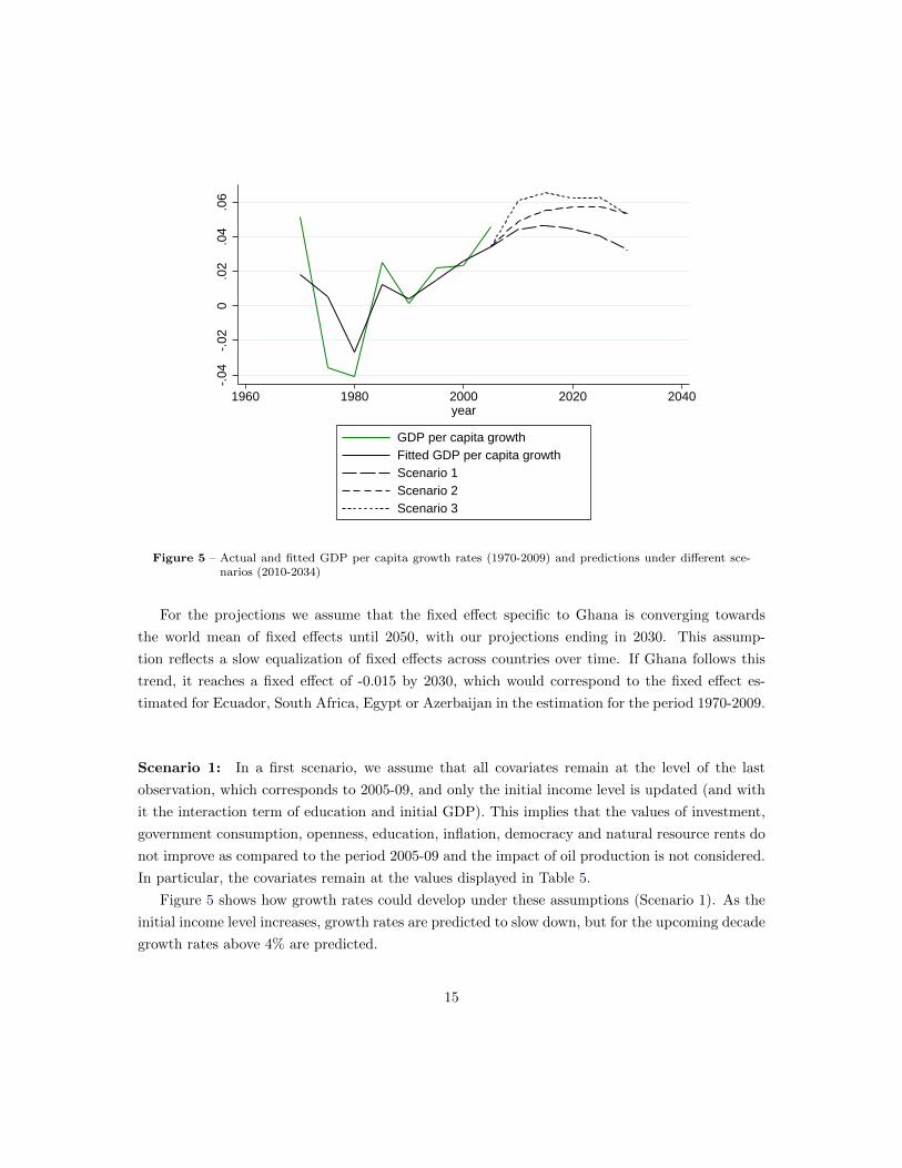
Figure 5 – Actual and fitted GDP per capita growth rates (1970-2009) and predictions under different sce-narios (2010-2034)

For the projections we assume that the fixed effect specific to Ghana is converging towards

the world mean of fixed effects until 2050, with our projections ending in 2030. This assump-

tion reflects a slow equalization of fixed effects across countries over time. If Ghana follows this

trend, it reaches a fixed effect of -0.015 by 2030, which would correspond to the fixed effect es-

timated for Ecuador, South Africa, Egypt or Azerbaijan in the estimation for the period 1970-2009.

Scenario 1: In a first scenario, we assume that all covariates remain at the level of the last

observation, which corresponds to 2005-09, and only the initial income level is updated (and with

it the interaction term of education and initial GDP). This implies that the values of investment,

government consumption, openness, education, inflation, democracy and natural resource rents do

not improve as compared to the period 2005-09 and the impact of oil production is not considered.

In particular, the covariates remain at the values displayed in Table 5.

Figure 5 shows how growth rates could develop under these assumptions (Scenario 1). As the

initial income level increases, growth rates are predicted to slow down, but for the upcoming decade

growth rates above 4% are predicted.

15

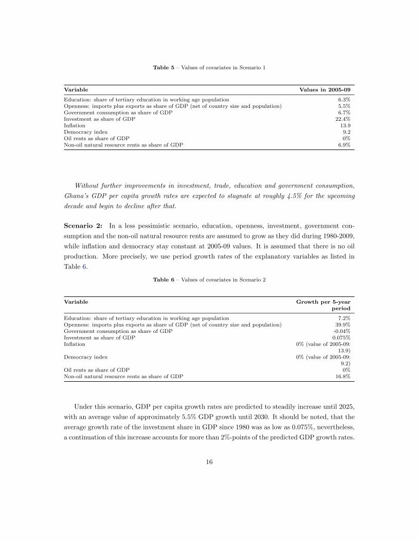
Table 5 – Values of covariates in Scenario 1

Variable Values in 2005-09

Education: share of tertiary education in working age population 6.3%Openness: imports plus exports as share of GDP (net of country size and population) 5.5%Government consumption as share of GDP 6.7%Investment as share of GDP 22.4%Inflation 13.9Democracy index 9.2Oil rents as share of GDP 0%Non-oil natural resource rents as share of GDP 6.9%

Without further improvements in investment, trade, education and government consumption,

Ghana’s GDP per capita growth rates are expected to stagnate at roughly 4.5% for the upcoming

decade and begin to decline after that.

Scenario 2: In a less pessimistic scenario, education, openness, investment, government con-

sumption and the non-oil natural resource rents are assumed to grow as they did during 1980-2009,

while inflation and democracy stay constant at 2005-09 values. It is assumed that there is no oil

production. More precisely, we use period growth rates of the explanatory variables as listed in

Table 6.

Table 6 – Values of covariates in Scenario 2

Variable Growth per 5-yearperiod

Education: share of tertiary education in working age population 7.2%Openness: imports plus exports as share of GDP (net of country size and population) 39.9%Government consumption as share of GDP -0.04%Investment as share of GDP 0.075%Inflation 0% (value of 2005-09:

13.9)Democracy index 0% (value of 2005-09:

9.2)Oil rents as share of GDP 0%Non-oil natural resource rents as share of GDP 16.8%

Under this scenario, GDP per capita growth rates are predicted to steadily increase until 2025,

with an average value of approximately 5.5% GDP growth until 2030. It should be noted, that the

average growth rate of the investment share in GDP since 1980 was as low as 0.075%, nevertheless,

a continuation of this increase accounts for more than 2%-points of the predicted GDP growth rates.

16

0.0

05.0

1.0

15E

xpec

ted

oil r

ents

in G

DP

2010 2015 2020 2025 2030Year

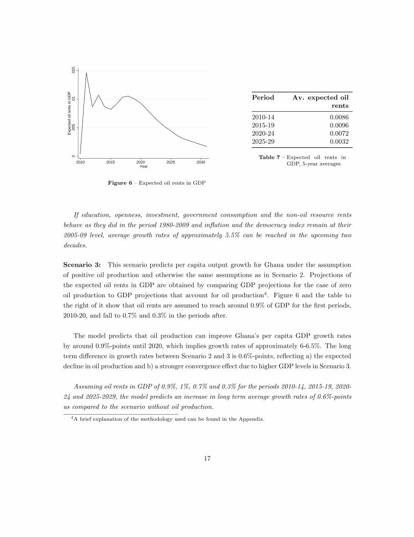
Figure 6 – Expected oil rents in GDP

Period Av. expected oilrents

2010-14 0.00862015-19 0.00962020-24 0.00722025-29 0.0032

Table 7 – Expected oil rents inGDP, 5-year averages

If education, openness, investment, government consumption and the non-oil resource rents

behave as they did in the period 1980-2009 and inflation and the democracy index remain at their

2005-09 level, average growth rates of approximately 5.5% can be reached in the upcoming two

decades.

Scenario 3: This scenario predicts per capita output growth for Ghana under the assumption

of positive oil production and otherwise the same assumptions as in Scenario 2. Projections of

the expected oil rents in GDP are obtained by comparing GDP projections for the case of zero

oil production to GDP projections that account for oil production4. Figure 6 and the table to

the right of it show that oil rents are assumed to reach around 0.9% of GDP for the first periods,

2010-20, and fall to 0.7% and 0.3% in the periods after.

The model predicts that oil production can improve Ghana’s per capita GDP growth rates

by around 0.9%-points until 2020, which implies growth rates of approximately 6-6.5%. The long

term difference in growth rates between Scenario 2 and 3 is 0.6%-points, reflecting a) the expected

decline in oil production and b) a stronger convergence effect due to higher GDP levels in Scenario 3.

Assuming oil rents in GDP of 0.9%, 1%, 0.7% and 0.3% for the periods 2010-14, 2015-19, 2020-

24 and 2025-2029, the model predicts an increase in long term average growth rates of 0.6%-points

as compared to the scenario without oil production.

4A brief explanation of the methodology used can be found in the Appendix.

17

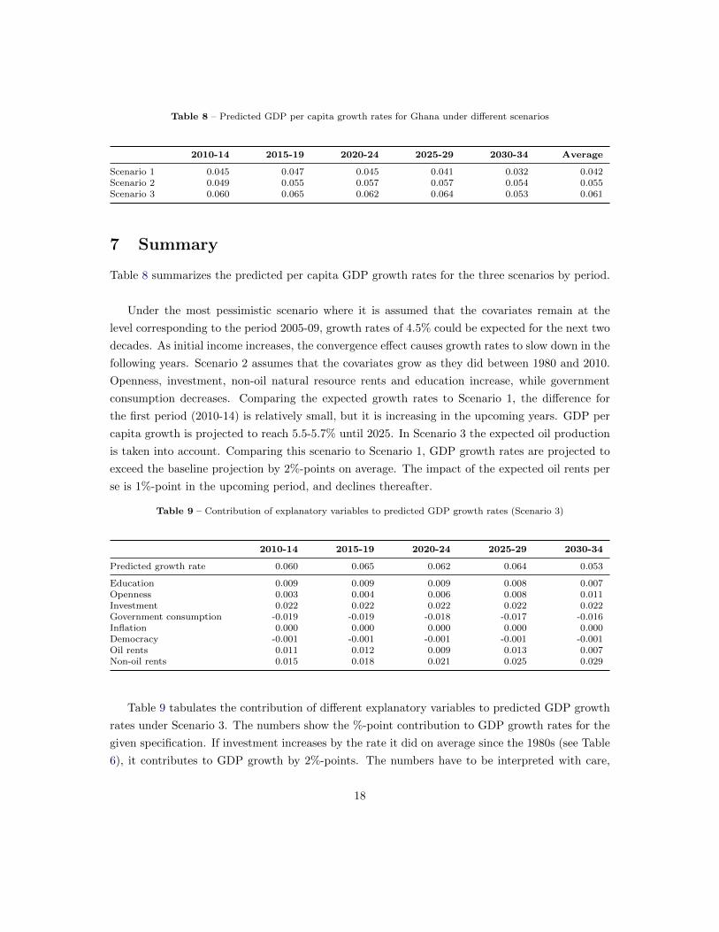
Table 8 – Predicted GDP per capita growth rates for Ghana under different scenarios

2010-14 2015-19 2020-24 2025-29 2030-34 Average

Scenario 1 0.045 0.047 0.045 0.041 0.032 0.042Scenario 2 0.049 0.055 0.057 0.057 0.054 0.055Scenario 3 0.060 0.065 0.062 0.064 0.053 0.061

7 Summary

Table 8 summarizes the predicted per capita GDP growth rates for the three scenarios by period.

Under the most pessimistic scenario where it is assumed that the covariates remain at the

level corresponding to the period 2005-09, growth rates of 4.5% could be expected for the next two

decades. As initial income increases, the convergence effect causes growth rates to slow down in the

following years. Scenario 2 assumes that the covariates grow as they did between 1980 and 2010.

Openness, investment, non-oil natural resource rents and education increase, while government

consumption decreases. Comparing the expected growth rates to Scenario 1, the difference for

the first period (2010-14) is relatively small, but it is increasing in the upcoming years. GDP per

capita growth is projected to reach 5.5-5.7% until 2025. In Scenario 3 the expected oil production

is taken into account. Comparing this scenario to Scenario 1, GDP growth rates are projected to

exceed the baseline projection by 2%-points on average. The impact of the expected oil rents per

se is 1%-point in the upcoming period, and declines thereafter.

Table 9 – Contribution of explanatory variables to predicted GDP growth rates (Scenario 3)

2010-14 2015-19 2020-24 2025-29 2030-34

Predicted growth rate 0.060 0.065 0.062 0.064 0.053

Education 0.009 0.009 0.009 0.008 0.007Openness 0.003 0.004 0.006 0.008 0.011Investment 0.022 0.022 0.022 0.022 0.022Government consumption -0.019 -0.019 -0.018 -0.017 -0.016Inflation 0.000 0.000 0.000 0.000 0.000Democracy -0.001 -0.001 -0.001 -0.001 -0.001Oil rents 0.011 0.012 0.009 0.013 0.007Non-oil rents 0.015 0.018 0.021 0.025 0.029

Table 9 tabulates the contribution of different explanatory variables to predicted GDP growth

rates under Scenario 3. The numbers show the %-point contribution to GDP growth rates for the

given specification. If investment increases by the rate it did on average since the 1980s (see Table

6), it contributes to GDP growth by 2%-points. The numbers have to be interpreted with care,

18

however, as due to the dynamic nature of the model they do not imply that growth rates decline by

2%-points if investment fell to zero. A similarly high positive impact on growth rates is attributed

to the non-oil natural resource rents, while government consumption appears to be the variable

that reduces GDP growth rates by the largest extent. It should be noted, however, that the results

should be interpreted as long run effects and no predictions can be done for a short run perspective.

The democracy measure does have a very small and even negative impact on GDP growth and

it does not appear as a significant driver of growth. This fact can partially be explained by the

inclusion of fixed effects: To the extent that they are constant over time, institutional character-

istics, political stability and business environment are comprised in the fixed effects. Only the

part that changes over time can be addressed in the estimation. The persistent nature of institu-

tional characteristics usually leads to a low variation in the variables and therefore identification

is difficult.

19

References

Barro, R. J. (2003): “Determinants of Economic Growth in a Panel of Countries,” Annals of

Economics and Finance, 4(2), 231–274.

Bollen, K. (1990): “Political Democracy: Conceptual and Measurement Traps,” Studies In

Comparative International Development, 25, 7–24.

Hanushek, E., and L. Wossmann (2008): “The Role of Congnitive Skills in Economic Devel-

opment,” Journal of Economic Literature, 8(1), 1–14.

Heston, A., R. Summers, and B. Aten (2012): Penn World Table Version 7.1 Center for

International Comparisons of Production, Income and Prices at the University of Pennsylvania.

Lejarraga, I. (2010): “Roaring Tiger of Purring Pussycat: A Growth Diagnostics Study of

Ghana,” Development Research Department Chief Economist Complex, African Development

Bank.

Lutz, W., J. C. Cuaresma, and W. Sanderson (2008): “The demography of educational

attainment and economic growth,” Science, 319, 1047–1048.

Lutz, W., A. Goujon, S. K.C., and W. Sanderson (2007): “Reconstruction of population by

age, sex and level of educational attainment of 120 countries for 1970-2000,” Vienna Yearbook

of Population Research, 2007, 193–235.

Sauer, P., and M. Zagler (2012): “(In)equality in Education and Economic Development,”

Paper Prepared for the 32nd General Conference of The International Association for Research

of Income and Wealth Session 2D, [http://www.iariw.org/papers/2012/SauerPaper.pdf].

Teorell, J., N. Charron, M. Samanni, S. Holmberg, and B. Rothstein (2011): The

Quality of Government Dataset Version, 6Apr11,University of Gothenburg: The Quality of

Government Institute [http://www.qog.pol.gu.se].

World Bank (2013): Energizing Economic Growth in Ghana: Making the Power and Petroleum

Sectors Rise to the Challenge,Energy Group, Africa Region, The World Bank.

20

A Appendix

Table A.10 – Description of variables

Variable Description Source

Rule of Law A composition of various indicators measuring the extent to which agentshave confidence in and abide by the rules of society; it includes perceptionsof the incidence of crime, the effectiveness and predictability of judiciary,and the enforcement of contracts.

WGI

Government Effectiveness A composition of various indicators measuring the quality of public servicepositions, the quality of bureaucracy, the competence of civil servants, theindependence of the civil service from political pressures, and the credibilityof the governments commitment to policies.

WGI

Political Stability A composition of various indicators measuring the likelihood that thegovernment in power will be destabilized or overthrown by unconstitutionalor violent means, including domestic violence of terrorism.

WGI

Corruption A composition of various indicators measuring the perception of corruption,defined as the exercise of public power for private gain.

WGI

Indicators used to assess the institutional quality.

WGI is short for the World Bank Worldwide Governance Indicators

For a more detailed description see Teorell, Charron, Samanni, Holmberg, and Rothstein (2011)

21

ETHCOGMOZNGA

TGOMNGKEN

NPLCIV

BGDPHL

KGZZMB

JORBENMDASEN

ZWETJK

KHMMAR

CMRINDVNM

PRYPAKTZAUKRLKA

NICHTIGEO

IDNBOLNAMBHRTHAMYSTUNPER

DZAHND

SYRIRQKAZ

AZEECUZAFEGYGAB

RUSALB

SDNMKD

SGPCOL

GHA

ESTIRNGTM

PANBGRSAUDOMARM

HRVCHNTURJAMBRAMEXSLVBLRLTU

HUNARGURYSVK

SURPOL

LVASVNCZE

BELTCDPRTLUXTTOMLTCYPIRLKOR

CRICANAUS

NZLGNQFINESP

NLDDNKDEUGRCITA

CHEJPNAUTSWEFRA

USAGBR

ISRISLNOR

QAT

-.1 -.05 0 .05 .1 .15Estimated Fixed Effects

Figure A.7 – Fixed effects based on specification (5) in Table 2

22

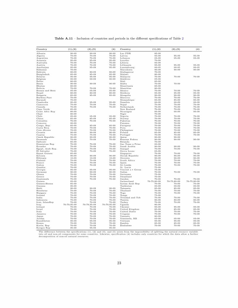
Table A.11 – Inclusion of countries and periods in the different specifications of Table 2

Country (1),(2) (3),(5) (4) Country (1),(2) (3),(5) (4)

Albania 90-09 90-09 90-09 Lao PDR 85-09Algeria 70-09 70-09 70-09 Latvia 95-09 95-09 95-09Argentina 70-09 70-09 70-09 Lebanon 05-09 05-09 05-09Armenia 95-09 95-09 95-09 Lesotho 70-09Australia 70-09 70-09 70-09 Liberia 00-09Austria 70-09 70-09 70-09 Lithuania 95-09 95-09 95-09Azerbaijan 95-09 95-09 95-09 Luxembourg 00-05 00-05 00-05Bahamas 70-09 Macedonia 90-09 90-09 90-09Bahrain 80-09 80-09 80-09 Madagascar 70-09Bangladesh 85-09 85-09 85-09 Malawi 80-09Belarus 95-09 95-09 95-09 Malaysia 70-09 70-09 70-09Belgium 00-09 00-09 00-09 Maldives 05-09Belize 80-09 Mali 85-09Benin 90-09 90-09 90-09 Malta 70-09 70-09Bhutan 80-09 Mauritania 85-09Bolivia 70-09 70-09 70-09 Mauritius 80-09Bosnia and Herz 05-09 05-09 05-09 Mexico 70-09 70-09 70-09Brazil 80-09 80-09 80-09 Moldova 95-09 95-09 95-09Bulgaria 85-09 85-09 85-09 Mongolia 90-09 90-09 90-09Burkina Faso 70-09 Morocco 70-09 70-09 70-09Burundi 70-09 Mozambique 85-09 85-09 85-09Cambodia 95-09 95-09 95-09 Namibia 00-09 00-09 00-09Cameroon 70-09 70-09 70-09 Nepal 70-09 70-09 70-09Canada 70-09 70-09 70-09 Netherlands 70-09 70-09 70-09Cape Verde 85-09 New Zealand 70-09 70-09 70-09Centr Afric Rep 80-09 Nicaragua 00-09 00-09 00-09Chad 80-09 Niger 70-09Chile 05-09 05-09 05-09 Nigeria 70-09 70-09 70-09China 85-09 85-09 85-09 Norway 70-09 70-09 70-09Colombia 70-09 70-09 70-09 Pakistan 70-09 70-09 70-09Comoros 00-09 Panama 70-09 70-09 70-09Congo, Rep. 85-09 85-09 85-09 Paraguay 70-09 70-09 70-09Costa Rica 70-09 70-09 70-09 Peru 70-09 70-09 70-09Cote dIvoire 70-09 70-09 70-09 Philippines 70-09 70-09 70-09Croatia 90-09 90-09 90-09 Poland 85-09 85-09 85-09Cyprus 75-09 75-09 75-09 Portugal 70-09 70-09 70-09Czech Republic 90-09 90-09 90-09 Qatar 90-09 90-09Denmark 70-09 70-09 70-09 Russian Federa 90-09 90-09 90-09Djibouti 85-09 Rwanda 70-09Dominican Rep 70-09 70-09 70-09 Sao Tome a Princ 00-09Ecuador 70-09 70-09 70-09 Saudi Arabia 90-09 90-09 90-09Egypt, Arab Rep. 70-09 70-09 70-09 Senegal 70-09 70-09 70-09El Salvador 70-09 70-09 70-09 Sierra Leone 05-09Equat Guinea 85-09 Singapore 70-09 70-09 70-09Estonia 90-09 90-09 90-09 Slovak Republic 90-09 90-09 90-09Ethiopia 10-09 10-09 10-09 Slovenia 90-09 90-09 90-09Finland 70-09 70-09 70-09 South Africa 70-09 70-09 70-09France 70-09 70-09 70-09 Spain 70-09 70-09 70-09Gabon 70-09 70-09 70-09 Sri Lanka 70-09 70-09 70-09Gambia 70-09 St. Lucia 75-09Georgia 95-09 95-09 95-09 Vincent a t Grena 75-09Germany 90-09 90-09 90-09 Sudan 70-09 70-09 70-09Ghana 70-09 70-09 70-09 Suriname 75-09Greece 70-09 70-09 70-09 Swaziland 70-09Guatemala 70-09 70-09 70-09 Sweden 70-09 70-09 70-09Guinea 05-09 Switzerland 70-75,80-09 70-75,80-09 70-75,80-09Guinea-Bissau 85-09 Syrian Arab Rep 70-09 70-09 70-09Guyana 95-09 Tajikistan 00-09 00-09 00-09Haiti 90-09 90-09 90-09 Tanzania 85-09 85-09 85-09Honduras 70-09 70-09 70-09 Thailand 70-09 70-09 70-09Hungary 70-09 70-09 70-09 Togo 70-09 70-09 70-09Iceland 70-09 70-09 70-09 Tonga 75-09India 70-09 70-09 70-09 Trinidad and Tob 70-09 70-09 70-09Indonesia 70-09 70-09 70-09 Tunisia 80-09 80-09 80-09Iran, IslamRep 70-09 70-09 70-09 Turkey 70-09 70-09 70-09Iraq 70-79,95-09 70-79,95-09 70-79,95-09 Uganda 80-09Ireland 70-09 70-09 70-09 Ukraine 95-09 95-09 95-09Israel 70-09 70-09 70-09 United Kingdom 85-09 85-09 85-09Italy 70-09 70-09 70-09 United States 70-09 70-09 70-09Jamaica 70-09 70-09 70-09 Uruguay 70-09 70-09 70-09Japan 70-09 70-09 70-09 Vanuatu 80-09Jordan 70-09 70-09 70-09 Venezuela, RB 05-09 05-09 05-09Kazakhstan 95-09 95-09 95-09 Vietnam 95-09 95-09 95-09Kenya 70-09 70-09 70-09 Zambia 85-09 85-09 85-09Korea, Rep 70-09 70-09 70-09 Zimbabwe 70-09 70-09 70-09Kyrgyz Rep 95-09 95-09 95-09

The difference between the specifications (1), (2) and (3), and (5) arises from the impossibility of splitting the natural resource variableinto oil and non-oil components for some countries. Likewise, specification (4) includes only countries for which the data allow a furtherdecomposition of non-oil natural resources.

23

CIV ZMB

COG

TZA

ETH

CMRGHA

BEN

GAB

ZWE

MOZ

TCD

GNQ

NGA TGOKEN

SENGHA

-.1

-.05

0.0

5.1

.15

Fix

ed E

ffect

s

-3 -2 -1 0 1 2Polititcal Stability

CIVZMB

COG

TZA

ETH

CMRGHA

BEN

GAB

ZWE

MOZ

TCD

GNQ

NGA TGOKEN

SENGHA

-.1

-.05

0.0

5.1

.15

Fix

ed E

ffect

s

-2 -1 0 1 2Corruption

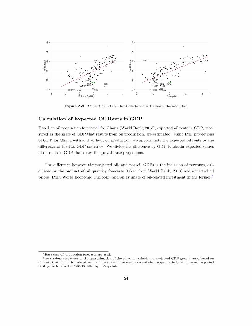
Figure A.8 – Correlation between fixed effects and institutional characteristics

Calculation of Expected Oil Rents in GDP

Based on oil production forecasts5 for Ghana (World Bank, 2013), expected oil rents in GDP, mea-

sured as the share of GDP that results from oil production, are estimated. Using IMF projections

of GDP for Ghana with and without oil production, we approximate the expected oil rents by the

difference of the two GDP scenarios. We divide the difference by GDP to obtain expected shares

of oil rents in GDP that enter the growth rate projections.

The difference between the projected oil- and non-oil GDPs is the inclusion of revenues, cal-

culated as the product of oil quantity forecasts (taken from World Bank, 2013) and expected oil

prices (IMF, World Economic Outlook), and an estimate of oil-related investment in the former.6

5Base case oil production forecasts are used.6As a robustness check of the approximation of the oil rents variable, we projected GDP growth rates based on

oil-rents that do not include oil-related investment. The results do not change qualitatively, and average expectedGDP growth rates for 2010-30 differ by 0.2%-points.

24