econ 219b psychology and economics: applications (lecture 4) · econ 219b psychology and economics:...

Econ 219B

Psychology and Economics: Applications

(Lecture 4)

Stefano DellaVigna

February 11, 2015

Outline

1. Laboratory Experiments on Present Bias II

2. Methodology: Errors in Applying Present-Biased Preferences

3. Reference Dependence: Introduction

4. Reference Dependence: Housing I

5. Methodology: Bunching-Based Evidence of Reference Dependence

6. Reference Dependence: Housing II

7. Reference Dependence: Tax Elusion

8. Reference Dependence: Goals

9. Reference Dependence: Mergers

1 Laboratory Experiments on Present Bias II

• Recent improved experimental design: Andreoni and Sprenger (AS, AER2012)

• To deal with Problem 1 (Credibility), emphasize credibility— All sooner and later payments, including those for t = 0, were placedin subjects’ campus mailboxes.

— Subjects were asked to address the envelopes to themselves at theircampus mailbox, thus minimizing clerical errors

— Subjects were given the business card of Professor James Andreoni andtold to call or e-mail him if a payment did not arrive

• Potential drawback: Payment today take places at end of day— Other experiments: post-dated checks

• To deal with Problem 3 (Concave Utility), design to estimate concavity:— Subject allocate share of money to earlier versus later choice

— - That is, interior solutions, not just corner solutions

— Vary interest rate between earlier and later choice to back out concavity

• Example of choice screenshot

• Main result: No evidence of present bias

• What about Problem 2 (Money vs. Consumption)?— One solution: Do experiments with goods to be consumed right away:

∗ Low- and High-brow movies (Read and Loewenstein, 1995)∗ Squirts of juice for thirsty subjects (McClure et al., 2005)

— Problem: Harder to invoke linearity of utility when using goods asopposed to money

• Augenblick, Niederle, and Sprenger (QJE Forthcoming): Address problemby having subjects intertemporally allocate effort

— 102 subjects have to complete boring task

• — Experiment over multiple weeks, complete online

— Pay largely at the end to reduce attrition

— Week 1: Choice allocation of job between weeks 2 and 3

— Week 2: Choose again allocation of job between weeks 2 and 3

— — Do subjects revise the choice?

— As in AS, choice of interior solution, and varied ‘interest rate’ betweenperiods

— Also do monetary discounting

• Result 1: On monetary discounting no evidence of present-bias

• Result 2: Clear evidence on effort allocation

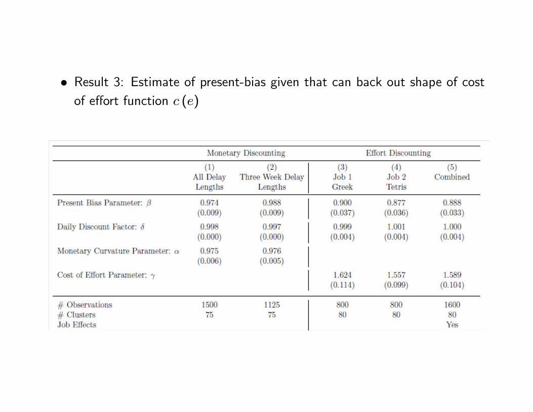
• Result 3: Estimate of present-bias given that can back out shape of costof effort function ()

• Dean and Sautmann (2014): Provide direct evidence on Problem 2(Money vs. Consumption)

— Elicit time preferences with standard money now versus money in thefuture questions

• — Observe shocks to ability to borrow and marginal utility of income

— Do those affect the choices in price list?

— If so, clearly we are not capturing but rather or 0

— Estimate MRS from questions above, relate to adverse income shock

• — Related to savings shock

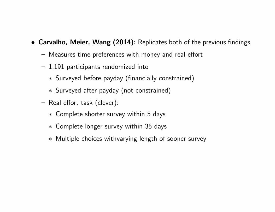
• Carvalho, Meier, Wang (2014): Replicates both of the previous findings— Measures time preferences with money and real effort

— 1,191 participants rendomized into

∗ Surveyed before payday (financially constrained)∗ Surveyed after payday (not constrained)

— Real effort task (clever):

∗ Complete shorter survey within 5 days∗ Complete longer survey within 35 days∗ Multiple choices withvarying length of sooner survey

• Replicates Dean and Sautmann result on financial choices

• Replicates Augenblick et al. on real effort

2 Methodology: Errors in Applying Present-Biased

Preferences

• Present-Bias model very successful• Quick adoption at cost of incorrect applications• Four common errors

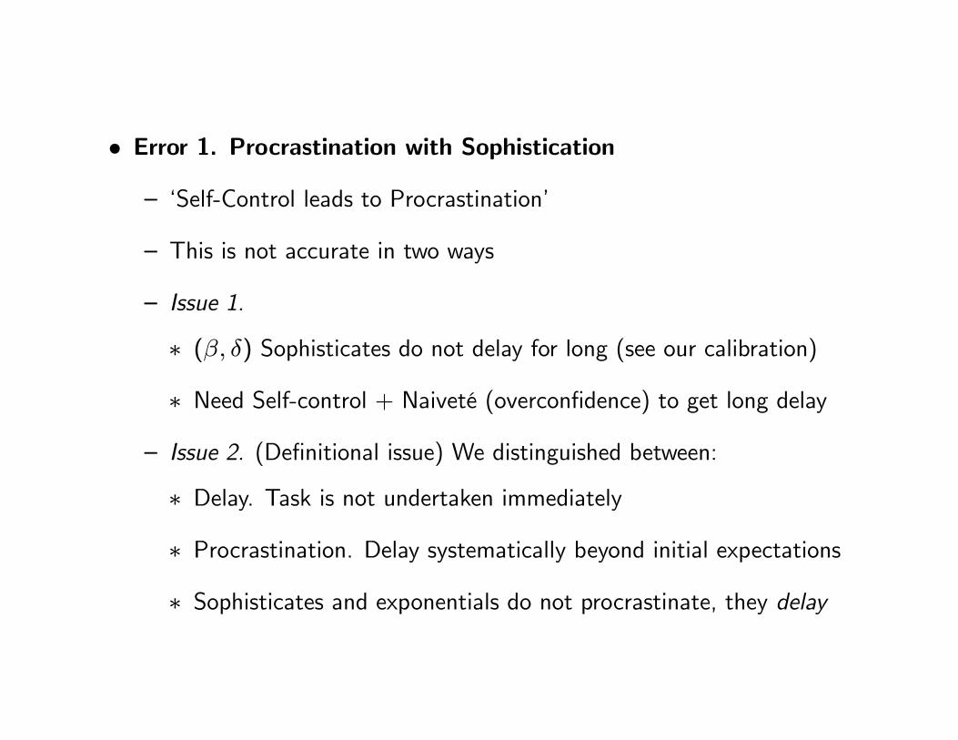
• Error 1. Procrastination with Sophistication— ‘Self-Control leads to Procrastination’

— This is not accurate in two ways

— Issue 1.

∗ ( ) Sophisticates do not delay for long (see our calibration)∗ Need Self-control + Naiveté (overconfidence) to get long delay

— Issue 2. (Definitional issue) We distinguished between:

∗ Delay. Task is not undertaken immediately∗ Procrastination. Delay systematically beyond initial expectations∗ Sophisticates and exponentials do not procrastinate, they delay

• Error 2. Naives with Yearly Decisions— ‘We obtain similar results for naives and sophisticates in our calibra-tions’

— Example 1. Fang, Silverman (IER, 2009)

— Single mothers applying for welfare. Three states:

1. Work

2. Welfare

3. Home (without welfare)

— Welfare dominates Home — So why so many mothers stay Home?

• — Model:

∗ Immediate cost (stigma, transaction cost) to go into welfare∗ For high enough, can explain transition∗ Simulate Exponentials, Sophisticates, Naives

— However: Simulate decision at yearly horizon.

— BUT: At yearly horizon naives do not procrastinate:

∗ Compare:· Switch now· Forego one year of benefits and switch next year

— Result:

∗ Very low estimates of ∗ Very high estimates of switching cost ∗ Naives are same as sophisticates

• — Conjecture: If allowed daily or weekly decision, would get:

∗ Naives fit much better than sophisticates∗ much closer to 1

∗ much smaller

— Example 2. Shui and Ausubel (2005) — Estimate Ausubel (1999)

∗ Cost of switching from credit card to credit card∗ Again: Assumption that can switch only every quarter∗ Results of estimates (again):· Quite low

· Naives do not do better than sophisticates· Very high switching costs

• Error 3. Present-Bias over Money— We discussed problem applied to experiments

— Same problem applies to models

∗ Notice: Transaction costs of switching in above models are realeffort, apply immediately

∗ Effort cost of attending gym also ‘real’ (not monetary)∗ Consumption-Savings models: Utility function of consumption , notincome

• Error 4. Getting the Intertemporal Payoff Wrong

— ‘Costs are in the present, benefits are in the future’

— ( ) models very sensitive to timing of payoffs

— Sometimes, can easily turn investment good into leisure good

— Need to have strong intuition on timing

— Example: Paper on nuclear plants as leisure goods

∗ Immediate benefits of energy

∗ Delayed cost to environment

— BUT: ‘Immediate’ benefits come after 10 years of construction costs!

3 Reference Dependence: Introduction

• Kahneman and Tversky (EMA 1979) – Anomalous behavior in experi-ments:

1. Concavity over gains. Given $1000, A=(500,1) Â B=(1000,0.5;0,0.5)

2. Convexity over losses. Given $2000, C=(-1000,0.5;0,0.5) Â D=(-500,1)

3. Framing Over Gains and Losses. Notice that A=D and B=C

4. Loss Aversion. (0,1) Â (-8,.5;10,.5)

5. Probability Weighting. (5000,.001) Â (5,1) and (-5,1) Â (-5000,.001)

• Can one descriptive model theory fit these observations?

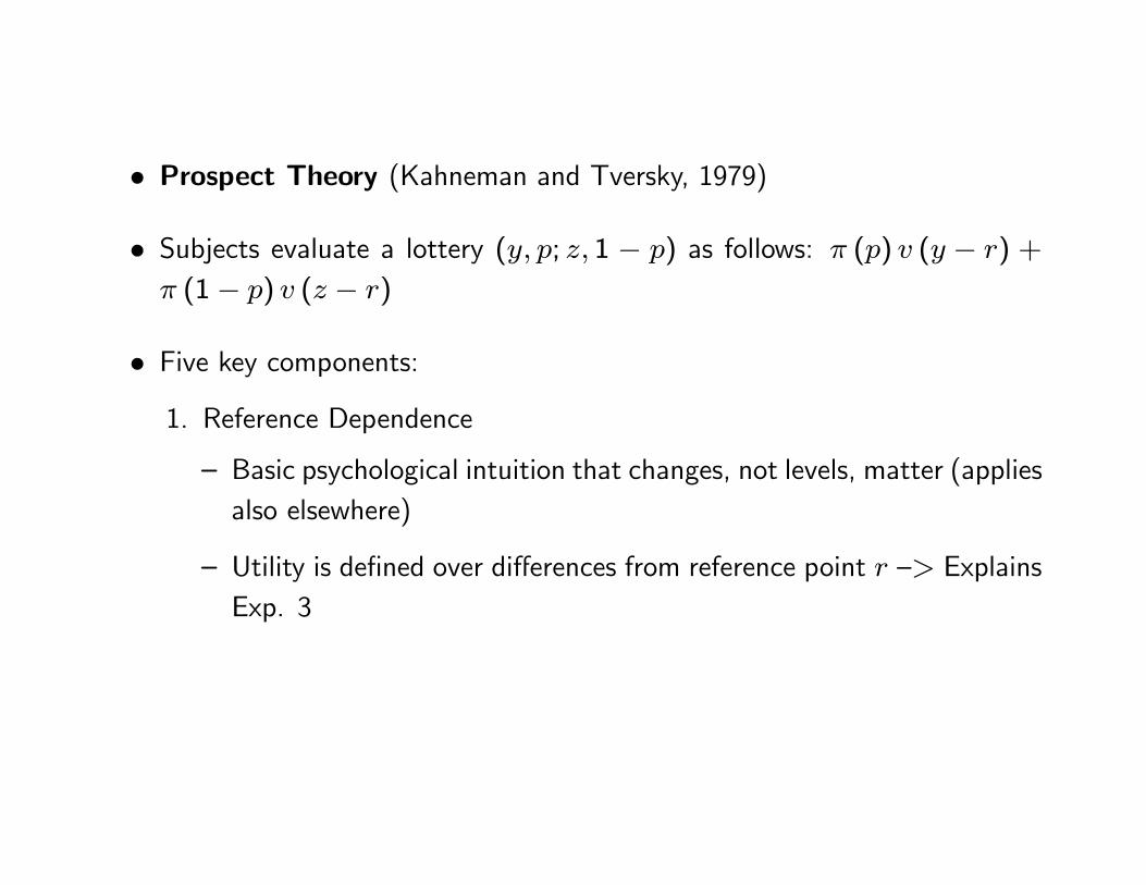
• Prospect Theory (Kahneman and Tversky, 1979)

• Subjects evaluate a lottery ( ; 1 − ) as follows: () ( − ) +

(1− ) ( − )

• Five key components:1. Reference Dependence

— Basic psychological intuition that changes, not levels, matter (appliesalso elsewhere)

— Utility is defined over differences from reference point — ExplainsExp. 3

2. Diminishing sensitivity.

— Concavity over gains of — Explains (500,1)Â(1000,0.5;0,0.5)— Convexity over losses of — Explains (-1000,0.5;0,0.5)Â(-500,1)

3. Loss Aversion — Explains (0,1) Â (-8,.5;10,.5)

4. Probability weighting function non-linear — Explains (5000,.001) Â(5,1) and (-5,1) Â (-5000,.001)

• Overweight small probabilities + Premium for certainty

5. Narrow framing (Barberis, Huang, and Thaler, 2006; Rabin andWeizsäcker,2011)

— Consider only risk in isolation (labor supply, stock picking, house sale)

— Neglect other relevant decisions

• Tversky and Kahneman (1992) propose calibrated version

() =

((− )88 if ≥ ;

−225 (− (− ))88 if

and

() =65³

65 + (1− )65´165

• Reference point ?

• Open question — depends on context

• Koszegi-Rabin (2006 on): personal equilibrium with rational expectationoutcome as reference point

• Most field applications use only (1)+(3), or (1)+(2)+(3)

() =

(− if ≥ ;

(− ) if

• Assume backward looking reference point depending on context

4 Reference Dependence: Housing I

• Start from old-school reference-dependence paper

• Two typical ingredients:1. Backward-looking reference points (status quo, focal point, or pastoutcome)

2. ‘Informal’ test — No model

• Genesove-Mayer (QJE, 2001)1. For houses sales, natural reference point is previous purchase price

— Validation: 75% of home owners remember exactly the purchaseprice of their home (survey evidence from our door-to-door surveys)

2. Loss Aversion — Unwilling to sell house at a loss

— Will ask for higher price if at a loss relative to pruchase price

• Evidence: Data on Boston Condominiums, 1990-1997

• Substantial market fluctuations of price

• Observe:— Listing price and last purchase price 0

— Observed Characteristics of property

— Time Trend of prices

• Define:— is market value of property at time

• Ideal Specification: = +1

0

³0 −

´+

= + + +∗ +

• However:— Do not observe given (unobserved quality)— Hence do not observe ∗

• Two estimation strategies to bound estimates. Model 1: = + +1

0(0 − − ) +

— This model overstate the loss for high unobservable homes (high )— Bias upwards in since high unobservable homes should have high

• Model 2: = ++ (0 − − )+10

(0 − − )+

• Estimates of impact on sale price

• Effect of experience: Larger effect for owner-occupied

• Some effect also on final transaction price

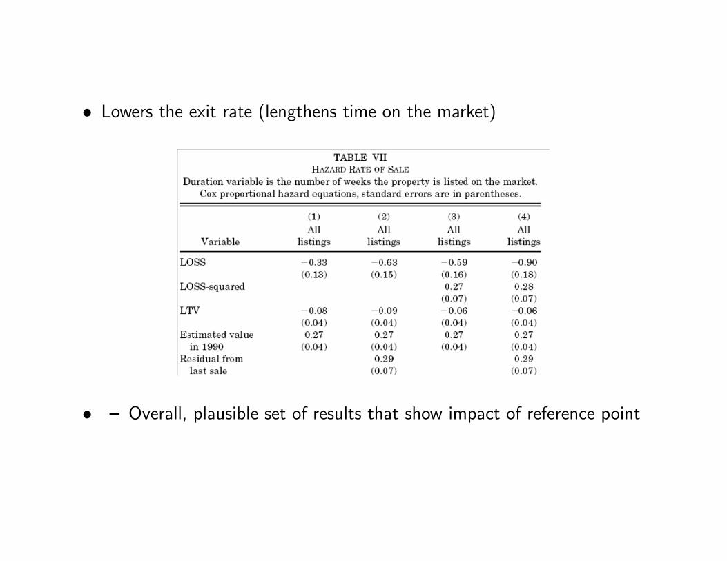
• Lowers the exit rate (lengthens time on the market)

• — Overall, plausible set of results that show impact of reference point

5 Methodology: Bunching-Based Evidence of Ref-

erence Dependence

• How does one identify reference-dependence?• Some Cases: Key role for diminishing sensitivity and probability weighting— Disposition effect: Diminishing sensitivity — more prone to sell win-ners (part of effect)

— Insurance: Prob. weighting — propensity to get low deductible

• Most Cases: Key role for loss aversion• Common element for several papers:— Well-defined, backward-looking reference point

— Optimal effort choice ∗

— Cost of effort ()

— Return of effort reference point

• Individual maximizesmax

+ [− ]− () for ≥

max

+ [− ]− () for

• Derivative of utility function:1 + − 0 (∗) for ≥

1 + − 0 (∗) for

— Discontinuity in marginal utility of effort

— Implication 1 — Bunching at ∗ =

— Implication 2 — Missing mass of distribution for compared to

• Older literature does not purse this, new literature does— Bunching is much harder to explain with alternative models

— Shift in mass can generally be well identified too under assumptions ofcontiuity of distribution

• Examine four related applications:1. Housing (where test is not formalized)

— Effort: How hard to ‘push’ the house

— Reference point: Purchase price

2. Tax filing

— Effort: Tax elusion

— Reference point: Withholding amount

3. Marathon running

— Effort: Running

— Reference point: Round goal

4. Merger

— Effort: Pushing for higher price

— Reference point: 52-week high

• Two more related cases next lecture:5. Labor supply

— Effort: Work more hours

— Reference point: Expected daily earnings?

6. Job search

— Effort: Search for a job

— Reference point: Recent average earnings

6 Reference Dependence: Housing II

• Return to Housing case, formalize intuition.— Seller chooses price at sale

— Higher Price

∗ lowers probability of sale ( ) (hence 0 ( ) 0)

∗ increases utility of sale ( )— If no sale, utility is ( ) (for all relevant )

• Maximization problem:max

( ) ( ) + (1− ( ))

• F.o.c. implies = ( ∗) 0 ( ∗) = −0( ∗)( ( ∗)− ) =

• Interpretation: Marginal Gain of increasing price equals Marginal Cost• S.o.c are

20( ∗) 0 ( ∗) + ( ∗) 00 ( ∗) + 00( ∗)( ( ∗)− ) 0

• Need 00( ∗)( ( ∗)− ) 0 or not too positive

• Reference-dependent preferences with reference price 0 (with pure gain-loss utility):

( |0) =(

− 0 if ≥ 0; ( − 0) if 0

— (in this case, think of 0)

— Can write as

( ) = −0( )( − 0 − ) if ≥ 0

( ) = −0( )( ( − 0)− ) if 0

— Plot Effect on MG and MC of loss aversion

• Compare ∗=1 (equilibrium with no loss aversion) and ∗1 (equilibriumwith loss aversion)

• Case 1. Loss Aversion increase price ( ∗=1 0)

• Case 2. Loss Aversion induces bunching at = 0 ( ∗=1 0)

• Case 3. Loss Aversion has no effect ( ∗=1 0)

• General predictions. When aggregate prices are low:— High prices relative to fundamentals

— Bunching at purchase price 0— Lower probability of sale ( )

— Longer waiting on market

• Important to tie housing evidence to model

• Gagnon-Bartsch, Rosato, and Xia (2010): Re-analyze data— Some evidence on bunching

— Did not do shifting test

— Would be great to redo with data from recent recession

7 Reference Dependence: Tax Elusion

• Alex Rees-Jones (2014)• Important setting which can also differentiate from alternative model ofreference points:

— Utility has fixed jump (but no kink)

— Prediction of bunching

— BUT no prediction of shift in distribution

• Slides courtesy of Alex• Other relevant paper: Engstrom, P., Nordblom, K., Ohlsson, H., &Persson, A. (AEJ: Policy, forthcoming)

— Similar evidence, but focus on claiming deductions

Introduction Theory Main Results Assessing Alt. Theories Policy Impact Conclusion

Decision environment

Consider the decisions made in the process of filing tax returns.

Some tax-relevant behaviors are predetermined.E.g., withholding, labor supply.

But, conditional on predetermined behavior, the taxpayer can:1 Work to claim tax shelters for past behavior.2 Pursue additional tax shelters.

Sheltering reduces current tax payment, at a cost:

Evasion: e.g., income underreporting.Costs: expected future penalties, accounting effort, stigma, etc.

Avoidance: e.g., legal pursuit of credits, deductions.Costs: effort and attention.


Model of sheltering decisions

maxs∈R+

m(−bPM + s)︸︷︷︸utility over money

− c(s)︸︷︷︸cost of sheltering

bPM —“pre-manipulation” balance due, with PDF f PMb .

Determined by past labor supply decisions, tax payments,and many other factors.Primary assumption: f PM

b is continuous.

s — tax dollars sheltered.Assumes that sheltering can be precisely targeted.

c(·) — increasing, convex, and twice continuouslydifferentiable cost of sheltering.


Simple example with smooth utility

Consider a model abstracting from income effects:

maxs∈R+

(w − bPM + s)︸︷︷︸linear utility over money


Optimal sheltering is determined by the first-order condition:

1− c′(s∗) = 0

Optimal sheltering solution: s∗ = c′−1(1).

→ Distribution of balance due, b ≡ bPM − s∗, is a horizontalshift of the distribution of bPM .


PDF of pre-manipulation balance due


PDF of final balance due after sheltering


Loss-averse case

maxs∈R+

m(−bPM + s)︸︷︷︸utility over money


Loss-averse utility specification:

(w − bPM + s)︸︷︷︸consumption utility

+ n(−bPM + s − r)︸︷︷︸gain-loss utility

n(x) =

{ηx if x ≥ 0ηλx if x < 0


Optimal loss-averse sheltering

This model generates an optimal sheltering solution withdifferent behavior across three regions:

s∗(bPM) =

sH if bPM > sH − rbPM + r if bPM ∈

[sL − r , sH − r

]sL if bPM < sL − r

where sH ≡ c′−1(1 + ηλ) and sL ≡ c′−1(1 + η).

Sufficiently large bPM → high amount of sheltering.Sufficiently small bPM → low amount of sheltering.For an intermediate range, sheltering chosen to offset bPM .


PDF of pre-manipulation balance due


PDF of final balance due after loss-averse sheltering

Revenue effect of loss framing: sH − sL.


Goals of empirical analysis

We will now test these two predictions in IRS tax records, andquantify the revenue effect each implies.

Bunching prediction: Excess mass at gain/loss threshold.

Shifting prediction: Dist. of losses shifted relative to gains.

Need to address potential confounds:Nonrefundable creditsExtremely accurate tax forecastingFixed costs in the loss domainInteractions with tax preparersAvoidance of underwitholding penaltiesLiquidity constraints


Data description

Dataset: 1979-1990 SOI Panel of Individual Returns.Contains most information from Form 1040 and somerelated schedules.Randomized by SSNs.

Exclude observations filed from outside of the 50 states + DC,drawn from outside the sampling frame, observations before1979.

Exclude individuals with zero pre-credit tax due, individuals withzero tax prepayments.

Primary sample: ≈ 229k tax returns, ≈ 53k tax filers.


First look: distribution of nominal balance due


Quantifying excess mass

Approach motivated by Chetty, Friedman, Olsen, and Pistaferri(2011), who studied bunching behavior in an alternate setting.

Cj = α +

[7∑

i=1

βi · bij

]+ γ · I(bj = 0) + δ · I(bj > 0) + εj

Fits the histogram local to the referent with a 7th-orderpolynomial.

All values expressed in 1990 dollars.


Distribution of balance due near gain/loss threshold


(1) (2) (3) (4) (5)All AGI groups 1st AGI quartile 2nd AGI quartile 3rd AGI quartile 4th AGI quartile

γ: I(balance due = 0) 136.43*** 46.57*** 26.79*** 21.06*** 42.01***(18.46) (8.25) (6.95) (5.66) (4.15)

δ : I(balance due > 0) -16.26* -3.50 -4.20 -3.42 -5.14**(9.41) (4.21) (3.54) (2.89) (2.12)

α : Constant 99.57*** 33.43*** 27.21*** 21.94*** 16.99***(5.45) (2.44) (2.05) (1.67) (1.23)

Balance-due polynomial X X X X XN: Bins in histogram 201 201 201 201 201Observations 16348 5725 4553 3602 2468R2 0.490 0.479 0.259 0.209 0.489

Notes: Standard errors in parentheses. Similar estimates generated with bootstrapped

standard errors. * p < 0.10, ** p < 0.05, *** p < 0.01. Table with bootstrapped SEs

Results robust to alternative orders of the polynomial.Similar or stronger significance patterns for polynomials oforder one through ten.BIC selects 2nd-order polynomial, yields similar results.

These estimates can be used to bound sH − sL.


Estimates of shifting in loss domain

The estimates we’ve focused on thus far have been based onthe bunching prediction.

Now we will assess the shifting prediction.Complementary approach: estimates (sH − sL) from adifferent feature of the data.Different strengths and weaknesses.

Pros: uses more of the data, less danger that individuals nearzero are non-representative.

Cons: will rely more on functional form restrictions, moresusceptible to systematic differences in unobserved variables.


Excluding data at gain/loss threshold, loss-averse shelteringimplies:

fb(x) =

{f PMb (x + κ) if x < rf PMb (x + κ+ s) if x > r

κ ≡ sL, s ≡ sH − sL

Empirical approach: Use NLLS to fit a mixture of normaldistributions to the histogram, directly modeling shift.

Cj = Obs ·

[2∑

i=1

pi

σiφ

(bj + s · I(b > 0)− µ

σi

)]+ εj

Common mean assumed to preserve symmetry.Similar estimates generated by fitting skew-normaldistribution, but fit is worse.


Fit of predicted distributions

Estimate table


Rationalizing differences in magnitudes

What drives the differences in the bunching and shiftingestimates?

Primary explanation: assumption that sheltering can bemanipulated to-the-dollar.

Possible for some types of sheltering: e.g. direct evasion,choosing amount to give to charity, targeted capital losses.Not possible for many types of sheltering.Excess mass at zero will “leave out” individuals withoutfinely manipulable sheltering technologies.Potential solution: permit diffuse bunching “near” zero.


Sheltering-relevant behaviors at zero balance due

(1) (2) (3) (4) (5) (6)Adjustments Itemized Deduction Credits

> 0 Amount > 0 Amount > 0 AmountBalance due = 0 0.09*** 1138.38* 0.01 2015.49* 0.01 535.50

(0.03) (619.59) (0.03) (1112.42) (0.03) (493.06)

Balance due > 0 0.05*** 259.35*** -0.00 429.42*** -0.01*** 27.97(0.00) (76.24) (0.00) (99.31) (0.00) (29.76)

Filing-year fixed effects X X X X X X

Balance-due polynomial X X X X X X

Lagged-AGI polynomial X X X X X XN 148325 33935 148325 62441 148325 54223

Notes: OLS regressions with standard errors clustered at the individual level. Monetaryquantities expressed in 1990 dollars. Xs indicate the presence of filing-year fixedeffects, a third-order polynomial in lagged AGI, or a third-order polynomial in balancedue interacted with I(balance due > 0) to allow for discontinuity at zero. * p < 0.10, **p < 0.05, *** p < 0.01.


Distribution with fixed cost in loss domain

Back

8 Reference Dependence: Goal Setting

• Allen, Dechow, Pope, Wu (2014)• Reference point can be a goal• Marathon running: Round numbers as goals• Similar identification considering discontinuities in finishing times aroundround numbers

• Channel of effects: Speeding up if behind and can still make goal

• Evidence strongly consistent with model— Missing distribution to the right

— Some bunching

• Hard to back out loss aversion given unobservable cost of effort

9 Reference Dependence: Mergers

• Baker, Pan, Wurgler (JF 2012)• On the appearance, very different set-up:— Firm A (Acquirer)

— Firm T (Target)

• After negotiation, Firm A announces a price for merger with Firm T

— Price typically at a 20-50 percent premium over current price

— About 70 percent of mergers go through at price proposed

— Comparison price for often used is highest price in previous 52 weeks,52

— Example of how Cablevision (Target) trumpets deal

• Assume that Firm T chooses price , and A decides accept reject• As a function of price probability ( ) that deal is accepted (dependson perception of values of synergy of A)

• If deal rejected, go back to outside value • Then maximization problem is same as for housing sale:

max

( ) ( ) + (1− ( ))

• Can assume T reference-dependent with respect to

( |0) =(

− 52 if ≥ 52; ( − 52) if 52

• Obtain same predictions as in housing market• (This neglects possible reference dependence of A)• Baker, Pan, and Wurgler (2009): Test reference dependence in mergers— Test 1: Is there bunching around 52? (GM did not do this)

— Test 2: Is there effect of 52 on price offered?

— Test 3: Is there effect on probability of acceptance?

— Test 4: What do investors think? Use returns at announcement

• Test 1: Offer price around 52

— Some bunching, missing left tail of distribution

• Notice that this does not tell us how the missing left tail occurs:— Firms in left tail raise price to 52?

— Firms in left tail wait for merger until 12 months after past peak, so52 is higher?

— Preliminary negotiations break down for firms in left tail

• Would be useful to compare characteristics of firms to right and left of52

• Test 2: Kernel regression of price offered (Renormalized by price 30 daysbefore, −30 to avoid heterosked.) on 52 :

100 ∗ − −30−30

= +

"100 ∗ 52 − −30

−30

#+

• Test 3: Probability of final acquisition is higher when offer price is above52 (Skip)

• Test 4: What do investors think of the effect of 52?— Holding constant current price, investors should think that the higher52 the more expensive the Target is to acquire

— Standard methodology to examine this:

∗ 3-day stock returns around merger announcement: −1+1∗ This assumes investor rationality∗ Notice that merger announcements are typically kept top secret untillast minute — On announcement day, often big impact

• Regression (Columns 3 and 5):

−1+1 = +

−30+

where −30 is instrumented with 52−30

• Results very supportive of reference dependence hypothesis — Also alter-native anchoring story

10 Next Lecture

• Reference-Dependent Preferences— Labor Supply

— Job Search

— Finance

• Problem Set 2 due next week

econ 219b psychology and economics: applications (lecture 4) · econ 219b psychology and economics:...

Documents