econ 137 urban economics
TRANSCRIPT

Econ 137Urban Economics
Guillermo Ordonez, UCLA
Lecture Notes III

Econ 137 - Summer 2007 2
Questions for Lecture Notes III
Is there a land use pattern?
What is it like?
What determines the price of land?
What determines the pattern in the use of land?

Econ 137 - Summer 2007 3
The Leftover Principle
From Ricardo
From competition (and since land is fixed), households, manufacturers, offices, etc, would be willing to pay for land up to the profits of their activities in the land.

Econ 137 - Summer 2007 4
The Monocentric City
City with a Central Business District (CBD)
Assumptions:3 type of land uses (offices, manufacturing firms, residential)Central Export Node (Railroad terminal)Horse drawn wagons (goods from factory to railroad terminal)Hub-and-spoke streetcar system (for workers to factory)Agglomeration Economies (office industry)
Transport Technology is Key

Econ 137 - Summer 2007 5
The Monocentric City
Rural sector: Fertility of the land
Households: Accessibility to workplaces (i.e. commuting costs).
Manufacturing sector: Accessibility to consumers or suppliers. (i.e. distance to consumers or suppliers)
Information sector: Accessibility to information
What determine land prices?

Econ 137 - Summer 2007 6
Residential land
Households
Housing Service
ProvidersLand
Owners
Price for Housing
Bid- Rent for Residential Land
Land Price and Land use

Econ 137 - Summer 2007 7
Housing Prices (without substitution)NO consumer substitution:
1000 square- foot houses$300/month budget for typical HHCommuting cost = $20/mile per month
060120180240iii) Net income/month (300-(i)*20)10001000100010001000ii) Housing consumption (square feet)
00.060.120.180.24Price per Square-foot (iii/ii)
1512963i) Distance to city center (miles)Assumed Consumption Pattern
Linear housing price function [slope = -0.02$/sq. foot]

Econ 137 - Summer 2007 8
Housing price function (w/o substitution)Housing Price Function
0
0.05
0.1
0.15
0.2
0.25
0.3
0.35
0 3 6 9 12 15
Distance to center (in miles)
Pric
e of
hou
sin
Without substitution

Econ 137 - Summer 2007 9
Housing Prices (with substitution)
The household may decide whether to live at:A small house (less expensive in land).A big house (more expensive in land).
House size
Consumption
Indifference curve

Econ 137 - Summer 2007 10
Housing Pricing (with substitution)
House size
Consumption High relative price of houses
Low relative price of house
Small house
Big house

Econ 137 - Summer 2007 11
Housing Pricing (with substitution)Consumer substitution
As the price of land increases, people accept smaller houses.
060120180240iii) Net income/month (300-(i)*20)10001000750600500ii) Housing consumption (square feet)
00.060.160.300.48Price per Square-foot (iii/ii)
1512963i) Distance to city center (miles)Assumed Consumption Pattern
Convex housing price function

Econ 137 - Summer 2007 12
Housing price functionsHousing Price Function
0
0.1
0.2
0.3
0.4
0.5
0.6
0.7
0.8
0 3 6 9 12 15
Distance to center (in miles)
Pric
e of
hou
sin
Without substitution
With substitution

Econ 137 - Summer 2007 13
Residential land – Bid Rents (from production of houses)Fixed proportions:
( ) ( )
( ) id Rentsquare feet of housing [not land!!]nonland costs (to produce houses)price of housing (per squared feet)
distance from city center (blocks)
h h
h
h
R d P d H K
R d BHKPd
= −
=
===
=
Flexible proportions:( ) ( ) ( ) ( )h hR d P d H d K d= −

Econ 137 - Summer 2007 14
Housing-Price and Bid-Rent Functions$
Total Revenue = P(d)H
Cost of non-land inputs (K)
Bid-rent function
d* Miles to city center
Econ 137 - Summer 2007 15
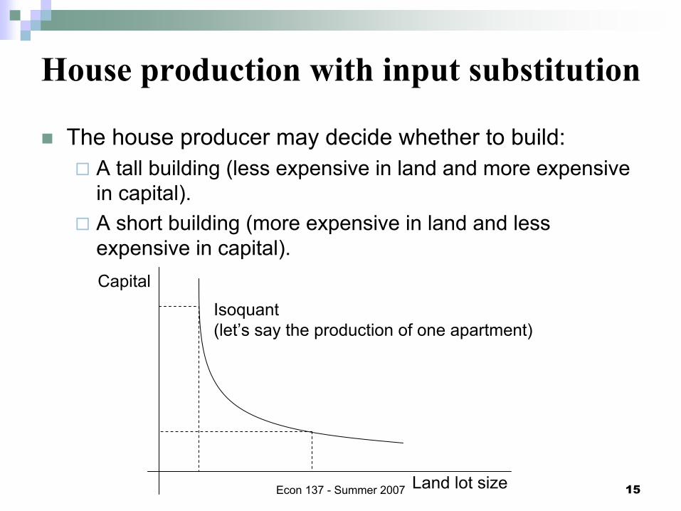
House production with input substitution
The house producer may decide whether to build:A tall building (less expensive in land and more expensive in capital).A short building (more expensive in land and less expensive in capital).
Land lot size
Capital
Isoquant(let’s say the production of one apartment)

Econ 137 - Summer 2007 16
House production with input substitution
Land lot size
Capital High relative price of land
Low relative price of land
Tall building
Short building

Econ 137 - Summer 2007 17
Consumer density
Consumer substitutionPrice of houses is high around the center, so people prefer smaller houses.
Factor substitutionProducers of houses substitute land by capital (relatively cheaper), producing tall buildings.
People packed in tall buildings and small apartments !!!

Econ 137 - Summer 2007 18
Important point !!!
The big effect is given by lot sizes.
If people accept to live in small houses in downtown (because the price of the houses), then real estate agents increase even more the price per square feet to extract all the surplus from the workers !!!!!
Recall we are tracking the price per square feet

Econ 137 - Summer 2007 19
Land for the manufacturing sectorManufacturers
Fixed Proportions and Constant Returns to Scale
( ) ( )
Price of goodsQuantity produced in one acre Production cost (noland inputs) of Q
distance from terminalwagon transport cost per unit per mile( ) land rent per acre t
m m m m
m
m
m
d P Q C tQd R d
PQCdtR d
= − − −
===
==
=
π
o bid

Econ 137 - Summer 2007 20
Land for the manufacturing sectorFixed Proportions and Constant Returns to ScaleProfits are zero ( )
Rent is determined by the terminal station location.
( )( )
m m m
m
R d P Q C tQdR d tQd
= − −
∂= −
∂
( ) 0m dπ =

Econ 137 - Summer 2007 21
Manufacturing Bid-Rent Curve
Distance from terminal
Rent (in $) Linear Bid-Rent Curve
Slope = -tQ

Econ 137 - Summer 2007 22
Manufacturing Bid-Rent Curve
Distance from terminal
Rent (in $)
If production function is flexible
Is the Bid-Rent Curve always linear?NO if the production is flexible
C(d) such that C’(d)>0
If production function is fixedLeontieff
This is because, as the factory approach to the centerit saves from distance (freight costs) and saves usingless land and more of other inputs

Econ 137 - Summer 2007 23
Offices Bid-Rent Curve
Travel costs in the information and consulting sector is subject to agglomeration economies.
While the manufacturing sector just has to transport the production to the terminal (one way), in the information sector employees have to return to offices (round trip)
In this case, the central location minimize total travel distance, which increases exponentially as the firm separates from the center.
The median location minimizes total travel distance

Econ 137 - Summer 2007 24
Principle of Median Location
Many input or output locations
Example: Pizza DeliveryUbiquitous inputs (tc=0)
Pizza price fixed (2 dollars/pizza, 1 pizza/consumer)
Each pizza sold requires one trip from store to buyer’s location
Many markets (differ in size and location)
Delivery cost per pizza = $2/mile

Econ 137 - Summer 2007 25
Principle of Median LocationOptimal Location?
Median Location has ½ of the monetary weight to the left and ½ to the right. MB of moving to the left or right (decrease in transport costs) is lower than the MC (increase in transport costs).
W X Y Z
0 1 2 92 8 1 10
$4 $16 $2 $20
Distance from W# of consumers
Monetary Weight

Econ 137 - Summer 2007 26
Principle of Median LocationOptimal Location?
Why not move from Y? to X?Total TC at X: $4 x1 + $16x0 + $2x1 + $20x8 = $168 Total TC at Y: $4 x2 + $16x1 + $2x0 + $20x7 = $164
What if 4 new consumers move to W?
W X Y Z
0 1 2 92 8 1 10
$4 $16 $2 $20
Distance from W# of consumers
Monetary Weight

Econ 137 - Summer 2007 27
Offices Bid-Rent Curve
Distance from center
Rent (in $) Concave Bid-Rent Curve
Basic assumption:Standard office

Econ 137 - Summer 2007 28
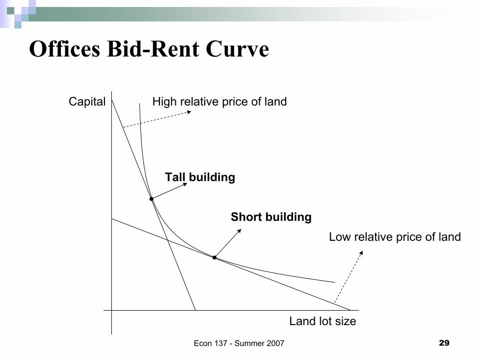
Offices Bid-Rent Curve
The firm may decide whether to locate the office at:A tall building (less expensive in land and more expensive in capital).A short building (more expensive in land and less expensive in capital).
Land lot size
CapitalIsoquant for offices
Econ 137 - Summer 2007 29
Offices Bid-Rent Curve
Land lot size
Capital High relative price of land
Low relative price of land
Tall building
Short building

Econ 137 - Summer 2007 30
Offices Bid-Rent Curve
Distance from center
Rent (in $) With factor substitutionClose to the center firms notonly have to pay more land
but also more capitalbecause of tall buildings
Without factorsubstitution
Why the two curves coincides here?

Econ 137 - Summer 2007 31
Land Use in the Monocentric City
Office bid-rent function
Manufacturing bid-rent function
Residential bid-rent function
Agricultural bid-rent function
Distance to city center
Land rent per acre
u0 u1 u2

Econ 137 - Summer 2007 32
Why these slopes?
Steeper bid- rents curves keep the center (more willingness to pay)
Slopes are determined by transport costs.
Office steeper because use people (workers walk)
Manufacturing use horses and wagoneers (trucks)
Resident commute of streetcars (buses or metro), which represent the lowest cost among the possibilities.

Econ 137 - Summer 2007 33
Land Use in the Monocentric CityOffice bid-rent function
Manufacturing bid-rent function
Residential bid-rent functionAgricultural bid-rent function
Distance to city center
Land rent per acre
u0 u1 u2
Office district
Manufacturing district
Residential district

Econ 137 - Summer 2007 34
Relaxing assumptions
Time cost of commuting
Non- commuting travel
Two- earner households
Spatial Variation in other locational attributes
Income differentials
Zoning

Econ 137 - Summer 2007 35
Relaxing assumptions
How the graph changes if we introduced a beltway?
Center
$
Beltway
Officesector
Officeworkers
Manufacturingworkers
Manufacturingworkers
Manufacturingsector

Econ 137 - Summer 2007 36
Summary Ch. 6 O’SullivanIn the monocentric city, manufacturers export their output in horse-drawn wagons to a central export node; office workers travel by foot from offices to a central market area to exchange information; commuters and shoppers travel to a hub-and-spoke streetcar system.The bid-rent curves are negatively sloped because of transportation cost, and convex because of factor substitution (and also consumer substitution in the case of housing).The office sector has higher transportation cost per mile, so its bid-rent function is relatively steep and office firms occupy the city central area.Employment is concentrated in the CBD because the cost of commuting from the suburbs to the CBD (via streetcars) is low relative to the cost of moving output from the suburbs to the city center.The urban land and labor markets are connected because labor demand is determined by the territory and density of the business sector, and labor supply is determined by the territory and density of the residential sector.

Econ 137 - Summer 2007 37
Cities are changingEmployers are more dispersed on the metropolitan area.
In the US, CBD concentrates 20% of total employment in MAIn the US, CBD concentrates 40% of total offices in MAPopulation (20% in 3 miles around CBD) and commuting

Econ 137 - Summer 2007 38
General characteristics of centers and subcenters in USNumerous in both new and old large MAsJobs dispersed rather than concentrated.Subcenters highly specializedHowever, centers still important.Density decreases as distance from center increases.Centers still more developed in face2face type of activities.Median workplace of the largest 100 metropolitan areas are about 7miles from city center

Econ 137 - Summer 2007 39
Urban densityVaries a lot across countries and cities in the USDensity gradient: Rate at which population decreases with distance
For example, 0.1 means the density decreases by 10% per mile from center.In average the density gradient in the US goes from 0.05 to 0.15
density / distancedensity
dg ∆=

Econ 137 - Summer 2007 40
Urban density
0.311963Baltimore, Milwakee, Philadelphia, and Rochester. Source, Mills (1972)
Average Density Gradient4 Metropolitan Areas
0.4019540.351958
0.6919200.6319300.5919400.501948
1.221880
0.8019100.9619001.061890
Avg GradientYear

Econ 137 - Summer 2007 41
Subcenters in Los AngelesConventional view of Los Angeles: “Endless urban sprawl, with employment and population dispersed throughout”
In fact, highly complex space economy characterized by a system of specialized centers, dispersed but yet strongly influenced by the pull of LA central area.
Up to WWII, metropolitan growth confined to LA county.
By 1965 suburbs well extended into Orange County to the south and San Fernando Valley to the north.
By 1980 suburbs well extended to Riverside and San Bernardino to the east and Ventura County to the western edge.

Econ 137 - Summer 2007 42
Subcenters in Los AngelesDefinition:
Density at least 25 workers / hectare
Total employment at least 10,000 workers
32 in 1980 (average 45 workers / hectare), including Downtown LA, Riverside, Ventura and San Bernardino
23 % of total metropolitan employment
4 largest centers form an arc from Santa Monica through downtown LA (Wilshire corridor, a giant center 19 miles long)
Downtown LA comprises ½ percent of region’s land area but contains 10% of workers and 31% jobs within centers.
Commutes to jobs within the center are longer than outside the center.

Econ 137 - Summer 2007 43
Subcenters in Los Angeles

Econ 137 - Summer 2007 44
Subcenters in Los Angeles

Econ 137 - Summer 2007 45
Subcenters in Los Angeles5 types
Mixed industrial (near a transport node, e.g. airport, port, marina). (LAX, Orange County Airport, Inglewood, Marina del Rey, etc.)
Mixed service (typically an independent center in the past) (Downtown LA, Santa Monica, Glendale, Santa Ana, Pasadena, Long Beach, Riverside, Ventura, San Bernardino, etc.)
Specialized manufacturing (Long Beach Airport, Burbank Airport, Hawthorne, Lawndale, etc.)
Service oriented (West LA, East LA, Anaheim, etc.)
Specialized entertainment (Hollywood and Burbank)

Econ 137 - Summer 2007 46
The rise of monocentric cities.
Improve in transportation technologyRule of thumb: “Radius of a city is the distance that can be traveled in one hour”Hub and spoke public transit system in the 19th century.Short CBDs
Before elevators, price of high floors were cheaper because they were rented at a discount that offset the costs of climbingfour or five floors of stairs.

Econ 137 - Summer 2007 47
The decline of monocentric cities.
Decentralization of manufacturingIntercity tucks. Trade off of moving away from center is between higher freight costs and lower wage.Since freight costs decrease, it’s better to move out from centers.From factories close to ports, railroads and city centers to factories close to highways, beltways and airports
Decentralization of officesAdvance of communications (a reduction in the need for face2face activities)

Econ 137 - Summer 2007 48
The decline of monocentric cities.
Decentralization of populationEvidence: Reduction in density gradientsRising income and change in consumption bundles (not clear)Decrease in commuting costs“Jobs follow workers to suburbs and workers follow jobs to suburbs”Others: Old housing at the center, high taxes, crime, low quality education, etc.

Econ 137 - Summer 2007 49
Summary Ch. 7 O’SullivanThe median job location is seven miles from the city center and the median residential location is eight miles.
Cities in the US are much less dense than cities in the rest of the world.
The key factors in the rise of large monocentric city were innovations in intraurban transportation that decreased the cost of commuting and innovations in construction that decreased the cost of tall buildings.
The key factors in the decentralization of jobs and people were increases in income and the development of the truck, the automobile and the highway system.
Between 1950 and 1990, the amount of urban land increased more thntwice as fast as the urban population.

Econ 137 - Summer 2007 50
Questions for Lecture Notes III
Is there a land use pattern?
What is it like?
What determines the price of land?
What determines the pattern in the use of land?

Econ 137 - Summer 2007 51
Practice Exercises - Lecture Notes III
O’SullivanChapter 6: Exercises 2, 3, 4 and 5.
Chapter 7: All exercises.