eco real-time system user guide - illumina...eco real-time pcr system user guide 3 real-time pcr...

FOR RESEARCH USE ONLY

ILLUMINA PROPRIETARYCatalog # EC-900-1001 Part # 15017157 Rev. ECurrent as of June 2011

Eco™ Real-Time PCR SystemUser Guide

INTENDED USE: The Eco Real-Time PCR System is intended to support the Real-Time polymerase chain reaction (PCR) application needs of life science researchers. This includes gene expression quantification and analysis as well as genotyping by allelic discrimination or high-resolution melting. The system is able to support other applications and protocols as well. Eco features high-quality optical and thermal modules to provide optimal performance and data quality. The system includes data analysis software that is preloaded on a netbook computer and provided on a separate USB drive for installation on additional computers as needed. Additional accessories and consumables are provided or available for purchase to ensure the best user experience.

Use of the Eco for specific intended uses, such as polymerase chain reaction (PCR), Real-Time qPCR, or high-resolution melting (HRM) may require the user to obtain rights from third parties. It is solely the user’s responsibility to obtain all rights necessary for the intended use of Eco.

This document and its contents are proprietary to Illumina, Inc. and its affiliates ("Illumina"), and are intended solely for the contractual use of its customer in connection with the use of the product(s) described herein and for no other purpose. This document and its contents shall not be used or distributed for any other purpose and/or otherwise communicated, disclosed, or reproduced in any way whatsoever without the prior written consent of Illumina. Illumina does not convey any license under its patent, trademark, copyright, or common-law rights nor similar rights of any third parties by this document.

The instructions in this document must be strictly and explicitly followed by qualified and properly trained personnel in order to ensure the proper and safe use of the product(s) described herein. All of the contents of this document must be fully read and understood prior to using such product(s).

FAILURE TO COMPLETELY READ AND EXPLICITLY FOLLOW ALL OF THE INSTRUCTIONS CONTAINED HEREIN MAY RESULT IN DAMAGE TO THE PRODUCT(S), INJURY TO PERSONS, INCLUDING TO USERS OR OTHERS, AND DAMAGE TO OTHER PROPERTY.

ILLUMINA DOES NOT ASSUME ANY LIABILITY ARISING OUT OF THE IMPROPER USE OF THE PRODUCT(S) DESCRIBED HEREIN (INCLUDING PARTS THEREOF OR SOFTWARE) OR ANY USE OF SUCH PRODUCT(S) OUTSIDE THE SCOPE OF THE EXPRESS WRITTEN LICENSES OR PERMISSIONS GRANTED BY ILLUMINA IN CONNECTION WITH CUSTOMER'S ACQUISITION OF SUCH PRODUCT(S).

FOR RESEARCH USE ONLY

© 2010-2011 Illumina, Inc. All rights reserved.

Illumina, illuminaDx, BeadArray, BeadXpress, cBot, CSPro, DASL, Eco, Genetic Energy, GAIIx, Genome Analyzer, GenomeStudio, GoldenGate, HiScan, HiSeq, Infinium, iSelect, MiSeq, Nextera, Sentrix, Solexa, TruSeq, VeraCode, the pumpkin orange color, and the Genetic Energy streaming bases are registered trademarks or trademarks of Illumina, Inc. All other brands and names contained herein are the property of their respective owners.

Eco Real-Time PCR System User Guide iii

Table of Contents

Chapter 1 Overview . . . . . . . . . . . . . . . . . . . . . . . . . . . . . . . . . . .1

Introduction . . . . . . . . . . . . . . . . . . . . . . . . . . . . . . . . . . . . . . . . . . . . . . . . . 2Real-Time PCR. . . . . . . . . . . . . . . . . . . . . . . . . . . . . . . . . . . . . . . . . . . . . . . 3Absolute and Relative Quantification . . . . . . . . . . . . . . . . . . . . . . . . . . . . . . 4Allelic Discrimination and High Resolution Melt . . . . . . . . . . . . . . . . . . . . . . 5Multiplexing Real-Time PCR . . . . . . . . . . . . . . . . . . . . . . . . . . . . . . . . . . . . 6

Chapter 2 Setup. . . . . . . . . . . . . . . . . . . . . . . . . . . . . . . . . . . . . .7

Unpack the Eco System. . . . . . . . . . . . . . . . . . . . . . . . . . . . . . . . . . . . . . . . 8Place Eco on the Bench . . . . . . . . . . . . . . . . . . . . . . . . . . . . . . . . . . . . . . . . 9Connect Eco. . . . . . . . . . . . . . . . . . . . . . . . . . . . . . . . . . . . . . . . . . . . . . . . 10Turn on the Eco System . . . . . . . . . . . . . . . . . . . . . . . . . . . . . . . . . . . . . . . 11Register your Eco . . . . . . . . . . . . . . . . . . . . . . . . . . . . . . . . . . . . . . . . . . . . 12

Chapter 3 Workflow . . . . . . . . . . . . . . . . . . . . . . . . . . . . . . . . . .13

Eco System Workflow . . . . . . . . . . . . . . . . . . . . . . . . . . . . . . . . . . . . . . . . 14Load the Plate . . . . . . . . . . . . . . . . . . . . . . . . . . . . . . . . . . . . . . . . . . . . . . 15Define a New Experiment . . . . . . . . . . . . . . . . . . . . . . . . . . . . . . . . . . . . . . 16Set Up the Plate Layout . . . . . . . . . . . . . . . . . . . . . . . . . . . . . . . . . . . . . . . 18Set Up the Thermal Profile . . . . . . . . . . . . . . . . . . . . . . . . . . . . . . . . . . . . . 24Monitor Run . . . . . . . . . . . . . . . . . . . . . . . . . . . . . . . . . . . . . . . . . . . . . . . . 25Analyze Data. . . . . . . . . . . . . . . . . . . . . . . . . . . . . . . . . . . . . . . . . . . . . . . . 26

Chapter 4 System Information. . . . . . . . . . . . . . . . . . . . . . . . . .39

Components . . . . . . . . . . . . . . . . . . . . . . . . . . . . . . . . . . . . . . . . . . . . . . . . 40Specifications and Environmental Requirements. . . . . . . . . . . . . . . . . . . . 42Symbols . . . . . . . . . . . . . . . . . . . . . . . . . . . . . . . . . . . . . . . . . . . . . . . . . . . 43

iv Part # 15017157 Rev E

Ta

ble

of

Co

nte

nts

Electromagnetic Compatibility. . . . . . . . . . . . . . . . . . . . . . . . . . . . . . . . . . .44Cleaning And Maintenance . . . . . . . . . . . . . . . . . . . . . . . . . . . . . . . . . . . . .45Return Process . . . . . . . . . . . . . . . . . . . . . . . . . . . . . . . . . . . . . . . . . . . . . .46

Chapter 5 Concepts . . . . . . . . . . . . . . . . . . . . . . . . . . . . . . . . . 47

Chapter 6 Glossary . . . . . . . . . . . . . . . . . . . . . . . . . . . . . . . . . . 49

Eco Real-Time PCR System User Guide 1

Ch

ap

ter 1

Overview

Introduction. . . . . . . . . . . . . . . . . . . . . . . . . . . . . . . . . . . . . . . . . . . . . . . . . . . . . . 2

Real-Time PCR . . . . . . . . . . . . . . . . . . . . . . . . . . . . . . . . . . . . . . . . . . . . . . . . . . . 3

Absolute and Relative Quantification . . . . . . . . . . . . . . . . . . . . . . . . . . . . . . . . . . . 4

Allelic Discrimination and High Resolution Melt . . . . . . . . . . . . . . . . . . . . . . . . . . . 5

Multiplexing Real-Time PCR . . . . . . . . . . . . . . . . . . . . . . . . . . . . . . . . . . . . . . . . . 6

2 Part # 15017157 Rev E

Ove

rvie

w Introduction

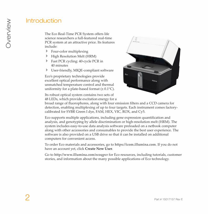
The Eco Real-Time PCR System offers life science researchers a full-featured real-time PCR system at an attractive price. Its features include:

Four-color multiplexingHigh Resolution Melt (HRM)Fast PCR cycling: 40-cycle PCR in 40 minutesUser-friendly, MIQE-compliant software

Eco’s proprietary technologies provide excellent optical performance along with unmatched temperature control and thermal uniformity for a plate-based format (± 0.1°C).

Its robust optical system contains two sets of 48 LEDs, which provide excitation energy for a broad range of fluorophores, along with four emission filters and a CCD camera for detection, enabling multiplexing of up to four targets. Each instrument comes factory-calibrated for SYBR Green I dye, FAM, HEX, VIC, ROX, and Cy5.

Eco supports multiple applications, including gene expression quantification and analysis, and genotyping by allele discrimination or high-resolution melt (HRM). The system includes easy-to-use data analysis software preloaded on a netbook computer along with other accessories and consumables to provide the best user experience. The software is also provided on a USB drive so that it can be installed on additional computers for convenient access.

To order Eco materials and accessories, go to https://icom.illumina.com. If you do not have an account yet, click Create New User.

Go to http://www.illumina.com/ecoqpcr for Eco resources, including tutorials, customer stories, and information about the many possible applications of Eco technology.

https://icom.illumina.com

http://www.illumina.com/ecoqpcr


Re

al-T

ime

PC

R

Real-Time PCR

Polymerase Chain Reaction (PCR) denotes the amplification of DNA templates catalyzed by DNA polymerase in the presence of primers, dNTPs, divalent cations (like Mg+2), and a buffer solution.

The ability to visualize and quantify the amplification of DNA as it occurs during PCR is called Real-Time PCR or Quantitative PCR (qPCR). This is made possible by the use of fluorescent chemistries, an optical system that can capture the emitted fluorescence at every PCR cycle, and software that can quantify the amplification.

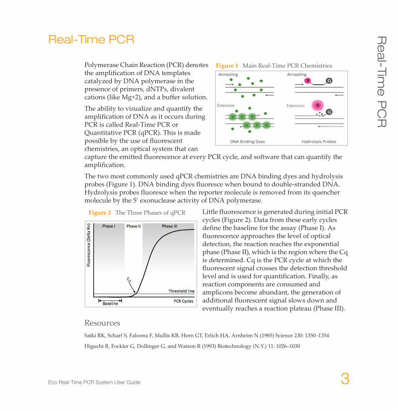
The two most commonly used qPCR chemistries are DNA binding dyes and hydrolysis probes (Figure 1). DNA binding dyes fluoresce when bound to double-stranded DNA. Hydrolysis probes fluoresce when the reporter molecule is removed from its quencher molecule by the 5’ exonuclease activity of DNA polymerase.

Little fluorescence is generated during initial PCR cycles (Figure 2). Data from these early cycles define the baseline for the assay (Phase I). As fluorescence approaches the level of optical detection, the reaction reaches the exponential phase (Phase II), which is the region where the Cq is determined. Cq is the PCR cycle at which the fluorescent signal crosses the detection threshold level and is used for quantification. Finally, as reaction components are consumed and amplicons become abundant, the generation of additional fluorescent signal slows down and eventually reaches a reaction plateau (Phase III).

ResourcesSaiki RK, Scharf S, Faloona F, Mullis KB, Horn GT, Erlich HA, Arnheim N (1985) Science 230: 1350–1354

Higuchi R, Fockler G, Dollinger G, and Watson R (1993) Biotechnology (N.Y.) 11: 1026–1030

Figure 1 Main Real-Time PCR Chemistries

Figure 2 The Three Phases of qPCR

4 Part # 15017157 Rev E

Ove

rvie

w Absolute and Relative Quantification

The two primary methods used to quantify nucleic acids by qPCR are the absolute and relative quantification methods.

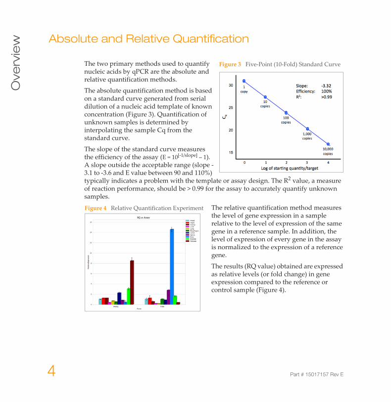
The absolute quantification method is based on a standard curve generated from serial dilution of a nucleic acid template of known concentration (Figure 3). Quantification of unknown samples is determined by interpolating the sample Cq from the standard curve.

The slope of the standard curve measures the efficiency of the assay (E = 10[-1/slope] – 1). A slope outside the acceptable range (slope -3.1 to -3.6 and E value between 90 and 110%) typically indicates a problem with the template or assay design. The R2 value, a measure of reaction performance, should be > 0.99 for the assay to accurately quantify unknown samples.

The relative quantification method measures the level of gene expression in a sample relative to the level of expression of the same gene in a reference sample. In addition, the level of expression of every gene in the assay is normalized to the expression of a reference gene.

The results (RQ value) obtained are expressed as relative levels (or fold change) in gene expression compared to the reference or control sample (Figure 4).

Figure 3 Five-Point (10-Fold) Standard Curve

Figure 4 Relative Quantification Experiment


Alle

lic D

isc

rimin

atio

n a

nd

Hig

h R

eso

lutio

n

Allelic Discrimination and High Resolution Melt

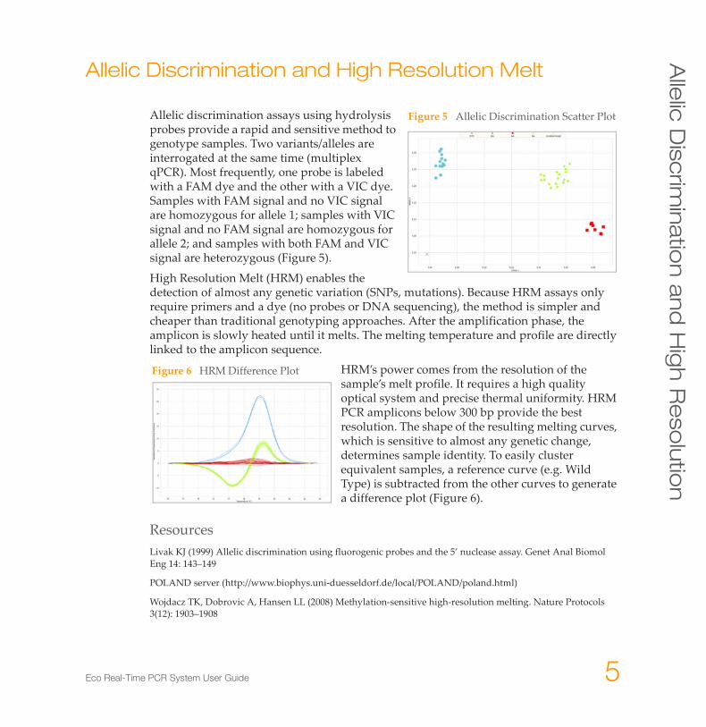
Allelic discrimination assays using hydrolysis probes provide a rapid and sensitive method to genotype samples. Two variants/alleles are interrogated at the same time (multiplex qPCR). Most frequently, one probe is labeled with a FAM dye and the other with a VIC dye. Samples with FAM signal and no VIC signal are homozygous for allele 1; samples with VIC signal and no FAM signal are homozygous for allele 2; and samples with both FAM and VIC signal are heterozygous (Figure 5).

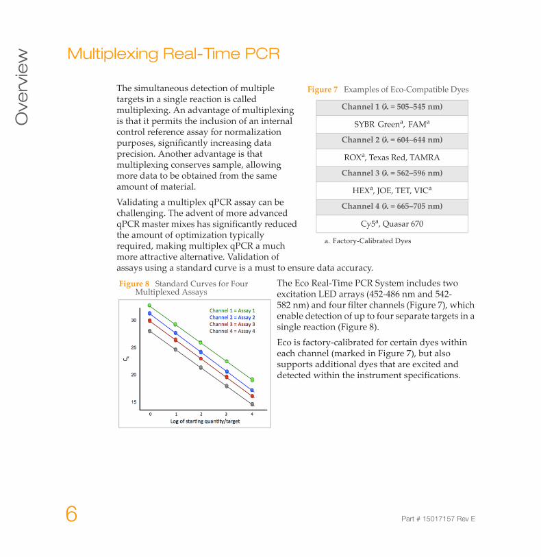
High Resolution Melt (HRM) enables the detection of almost any genetic variation (SNPs, mutations). Because HRM assays only require primers and a dye (no probes or DNA sequencing), the method is simpler and cheaper than traditional genotyping approaches. After the amplification phase, the amplicon is slowly heated until it melts. The melting temperature and profile are directly linked to the amplicon sequence.

HRM’s power comes from the resolution of the sample’s melt profile. It requires a high quality optical system and precise thermal uniformity. HRM PCR amplicons below 300 bp provide the best resolution. The shape of the resulting melting curves, which is sensitive to almost any genetic change, determines sample identity. To easily cluster equivalent samples, a reference curve (e.g. Wild Type) is subtracted from the other curves to generate a difference plot (Figure 6).

ResourcesLivak KJ (1999) Allelic discrimination using fluorogenic probes and the 5’ nuclease assay. Genet Anal Biomol Eng 14: 143–149

POLAND server (http://www.biophys.uni-duesseldorf.de/local/POLAND/poland.html)

Wojdacz TK, Dobrovic A, Hansen LL (2008) Methylation-sensitive high-resolution melting. Nature Protocols 3(12): 1903–1908

Figure 5 Allelic Discrimination Scatter Plot

Figure 6 HRM Difference Plot

6 Part # 15017157 Rev E

Ove

rvie

w Multiplexing Real-Time PCR

The simultaneous detection of multiple targets in a single reaction is called multiplexing. An advantage of multiplexing is that it permits the inclusion of an internal control reference assay for normalization purposes, significantly increasing data precision. Another advantage is that multiplexing conserves sample, allowing more data to be obtained from the same amount of material.

Validating a multiplex qPCR assay can be challenging. The advent of more advanced qPCR master mixes has significantly reduced the amount of optimization typically required, making multiplex qPCR a much more attractive alternative. Validation of assays using a standard curve is a must to ensure data accuracy.

The Eco Real-Time PCR System includes two excitation LED arrays (452-486 nm and 542-582 nm) and four filter channels (Figure 7), which enable detection of up to four separate targets in a single reaction (Figure 8).

Eco is factory-calibrated for certain dyes within each channel (marked in Figure 7), but also supports additional dyes that are excited and detected within the instrument specifications.

Channel 1 (λ = 505–545 nm)

SYBR Greena, FAMa

a. Factory-Calibrated Dyes

Channel 2 (λ = 604–644 nm)

ROXa, Texas Red, TAMRA

Channel 3 (λ = 562–596 nm)

HEXa, JOE, TET, VICa

Channel 4 (λ = 665–705 nm)

Cy5a, Quasar 670

Figure 7 Examples of Eco-Compatible Dyes

Figure 8 Standard Curves for Four Multiplexed Assays


Ch

ap

ter 2

Setup

Unpack the Eco System . . . . . . . . . . . . . . . . . . . . . . . . . . . . . . . . . . . . . . . . . . . . 8

Place Eco on the Bench . . . . . . . . . . . . . . . . . . . . . . . . . . . . . . . . . . . . . . . . . . . . 9

Connect Eco . . . . . . . . . . . . . . . . . . . . . . . . . . . . . . . . . . . . . . . . . . . . . . . . . . . . 10

Turn on the Eco System . . . . . . . . . . . . . . . . . . . . . . . . . . . . . . . . . . . . . . . . . . . 11

Register your Eco . . . . . . . . . . . . . . . . . . . . . . . . . . . . . . . . . . . . . . . . . . . . . . . . 12

8 Part # 15017157 Rev E

Se

tup Unpack the Eco System

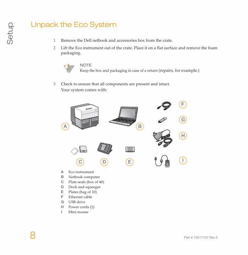
1 Remove the Dell netbook and accessories box from the crate.

2 Lift the Eco instrument out of the crate. Place it on a flat surface and remove the foam packaging.

3 Check to ensure that all components are present and intact.Your system comes with:

A Eco instrumentB Netbook computerC Plate seals (box of 40)D Dock and squeegeeE Plates (bag of 10)F Ethernet cableG USB driveH Power cords (2)I Mini mouse

NOTEKeep the box and packaging in case of a return (repairs, for example.)


Pla

ce

Ec

o o

n th

e B

en

ch

Place Eco on the Bench

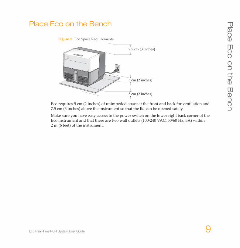
Figure 9 Eco Space Requirements

Eco requires 5 cm (2 inches) of unimpeded space at the front and back for ventilation and 7.5 cm (3 inches) above the instrument so that the lid can be opened safely.

Make sure you have easy access to the power switch on the lower right back corner of the Eco instrument and that there are two wall outlets (100-240 VAC, 50/60 Hz, 5A) within 2 m (6 feet) of the instrument.

7.5 cm (3 inches)

5 cm (2 inches)

5 cm (2 inches)

10 Part # 15017157 Rev E

Se

tup Connect Eco

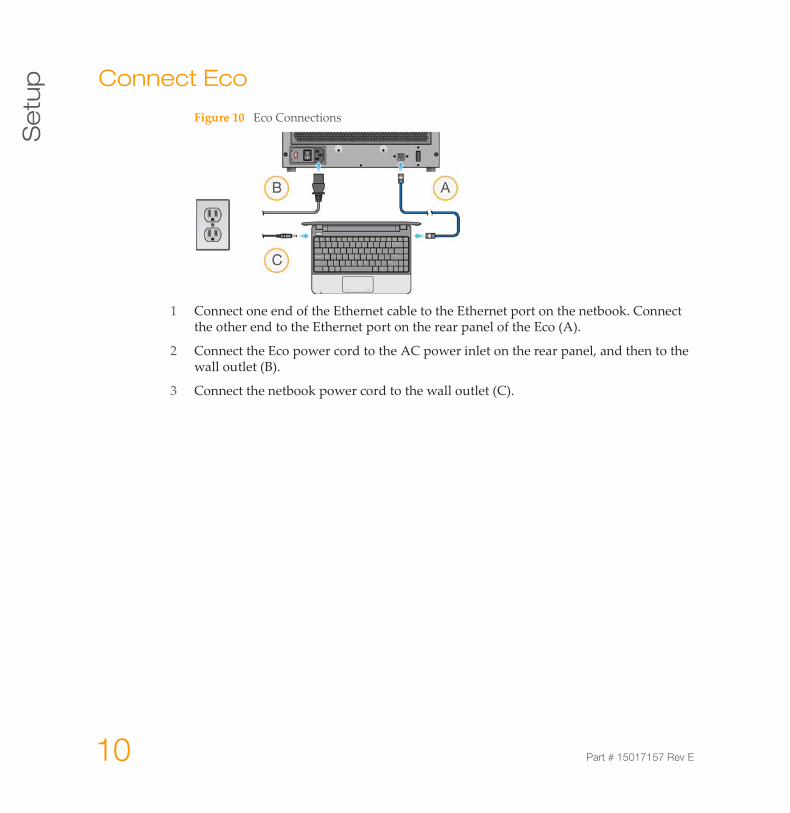
Figure 10 Eco Connections

1 Connect one end of the Ethernet cable to the Ethernet port on the netbook. Connect the other end to the Ethernet port on the rear panel of the Eco (A).

2 Connect the Eco power cord to the AC power inlet on the rear panel, and then to the wall outlet (B).

3 Connect the netbook power cord to the wall outlet (C).


Tu

rn o

n th

e E

co

Syste

m

Turn on the Eco System

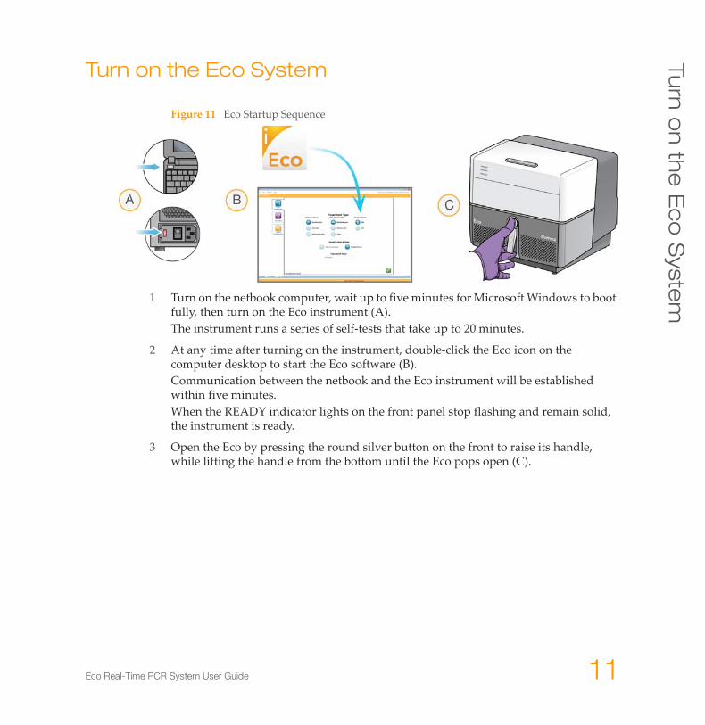
Figure 11 Eco Startup Sequence

1 Turn on the netbook computer, wait up to five minutes for Microsoft Windows to boot fully, then turn on the Eco instrument (A).The instrument runs a series of self-tests that take up to 20 minutes.

2 At any time after turning on the instrument, double-click the Eco icon on the computer desktop to start the Eco software (B).Communication between the netbook and the Eco instrument will be established within five minutes.When the READY indicator lights on the front panel stop flashing and remain solid, the instrument is ready.

3 Open the Eco by pressing the round silver button on the front to raise its handle, while lifting the handle from the bottom until the Eco pops open (C).

12 Part # 15017157 Rev E

Se

tup Register your Eco

Once your Eco system is set up and ready to use, register your Eco by going to http://www.ecoqpcr.com/register and completing a short questionnaire. Registering your Eco ensures that you will receive software updates in the future.

While you are visiting the web site, take advantage of the following online resources to support your research.

You are now ready to start an experiment. See Chapter 3, Workflow.

Eco Customer Support, knowledge database, warranty information, webinars, and seminar series

www.ecoqpcr.com/support

iCommunityA quarterly e-newsletter about, for, and by the Illumina community

www.illumina.com/icommunity

Online Ordering icom.illumina.com

Tradeshows, workshops, and meeting presence www.illumina.com/events

http://www.ecoqpcr.com/register

http://www.ecoqpcr.com/support

http://www.illumina.com/icommunity

http://icom.illumina.com

http://www.illumina.com/events


Ch

ap

ter 3

Workflow

Eco System Workflow . . . . . . . . . . . . . . . . . . . . . . . . . . . . . . . . . . . . . . . . . . . . . 14

Load the Plate. . . . . . . . . . . . . . . . . . . . . . . . . . . . . . . . . . . . . . . . . . . . . . . . . . . 15

Define a New Experiment . . . . . . . . . . . . . . . . . . . . . . . . . . . . . . . . . . . . . . . . . . 16

Set Up the Plate Layout . . . . . . . . . . . . . . . . . . . . . . . . . . . . . . . . . . . . . . . . . . . 18

Set Up the Thermal Profile. . . . . . . . . . . . . . . . . . . . . . . . . . . . . . . . . . . . . . . . . . 24

Monitor Run . . . . . . . . . . . . . . . . . . . . . . . . . . . . . . . . . . . . . . . . . . . . . . . . . . . . 25

Analyze Data . . . . . . . . . . . . . . . . . . . . . . . . . . . . . . . . . . . . . . . . . . . . . . . . . . . . 26

14 Part # 15017157 Rev E

Wo

rkflo

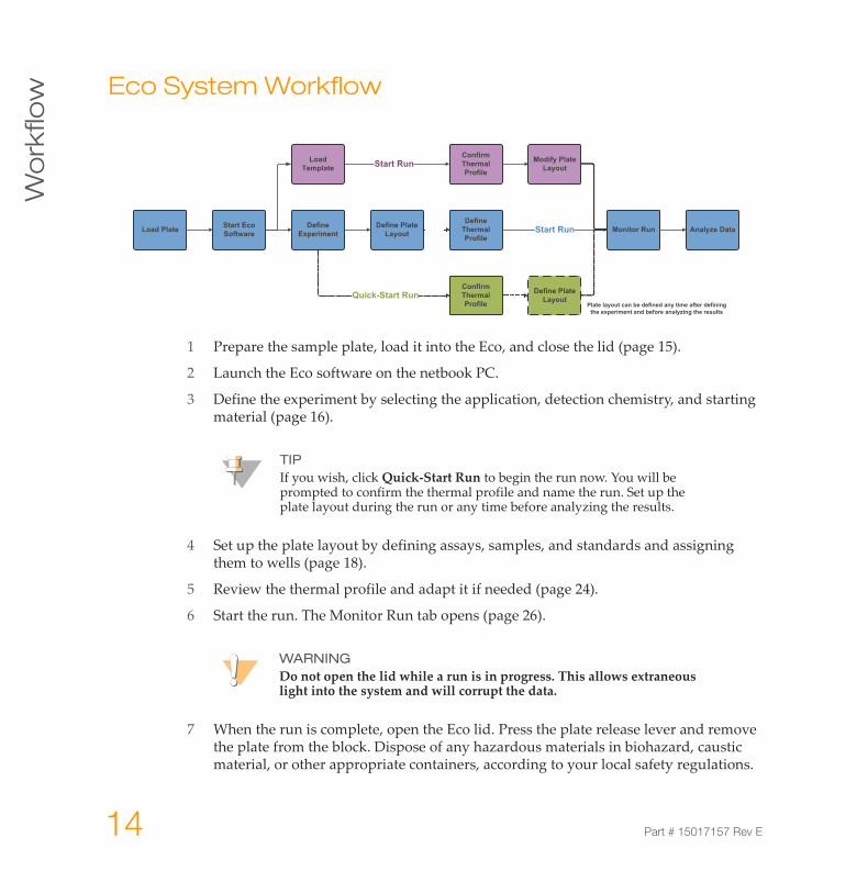
w Eco System Workflow

1 Prepare the sample plate, load it into the Eco, and close the lid (page 15).

2 Launch the Eco software on the netbook PC.

3 Define the experiment by selecting the application, detection chemistry, and starting material (page 16).

4 Set up the plate layout by defining assays, samples, and standards and assigning them to wells (page 18).

5 Review the thermal profile and adapt it if needed (page 24).

6 Start the run. The Monitor Run tab opens (page 26).

7 When the run is complete, open the Eco lid. Press the plate release lever and remove the plate from the block. Dispose of any hazardous materials in biohazard, caustic material, or other appropriate containers, according to your local safety regulations.

Start Eco Software

DefineExperiment

DefineThermal Profile

Define Plate Layout

Monitor Run Analyze DataStart Run

Plate layout can be defined any time after defining the experiment and before analyzing the results

Load Template Start Run

Load Plate Define Plate Layout

ConfirmThermal Profile

Quick-Start Run

ConfirmThermal Profile

Modify Plate Layout

TIPIf you wish, click Quick-Start Run to begin the run now. You will be prompted to confirm the thermal profile and name the run. Set up the plate layout during the run or any time before analyzing the results.

WARNINGDo not open the lid while a run is in progress. This allows extraneous light into the system and will corrupt the data.


Lo

ad

the

Pla

te

Load the Plate

1 Thaw all necessary reagents (templates, primers, probes, and master mix).

2 Turn on the netbook PC and Eco, then wait until the Eco Ready light is solid blue.

3 Confirm that the block and optical path are clear of visible contaminants and there is no physical damage to the system, such as dents, frayed cords, or damaged levers.

4 Place a 48-well plate into the Eco sample loading dock, aligning the notch with the matching indentation on the adapter.

5 Turn on the dock light and incline the dock to a comfortable angle for pipetting.

6 Pipette samples and qPCR reagents into the plate according to your protocol.

7 Seal the plate with an Eco optical seal. Holding the plate in place on the Eco sample loading dock, drag the squeegee firmly across the surface to ensure the seal is secure.

8 Place the plate adapter with your loaded and sealed plate into a compatible centrifuge rotor along with the second supplied plate adapter for balance. Centrifuge the plate at 250 g for 30 seconds. Do not spin more than 500 g. Verify that there are no air bubbles at the bottom of the wells.

9 Open the Eco lid and place the plate on the block, aligning the notch against the top-left corner.

10 Close the Eco lid. The heated lid automatically creates a seal around and on top of the plate to prevent evaporation. Proceed to define a new experiment.

WARNINGWear protective gloves and eyewear when handling any material that might be considered caustic or hazardous.

WARNINGForcing the plate into any other orientation could damage the instrument.

WARNINGBe careful not to touch the heated lid above the plate. It heats to 105°C (221°F) when the instrument is turned on and could result in burns.

16 Part # 15017157 Rev E

Wo

rkflo

w Define a New Experiment

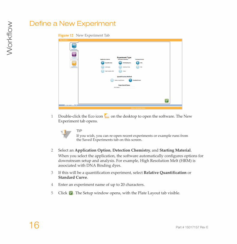
Figure 12 New Experiment Tab

1 Double-click the Eco icon on the desktop to open the software. The New Experiment tab opens.

2 Select an Application Option, Detection Chemistry, and Starting Material. When you select the application, the software automatically configures options for downstream setup and analysis. For example, High Resolution Melt (HRM) is associated with DNA Binding dyes.

3 If this will be a quantification experiment, select Relative Quantification or Standard Curve.

4 Enter an experiment name of up to 20 characters.

5 Click . The Setup window opens, with the Plate Layout tab visible.

TIPIf you wish, you can re-open recent experiments or example runs from the Saved Experiments tab on this screen.


De

fine

a N

ew

Ex

pe

rime

nt

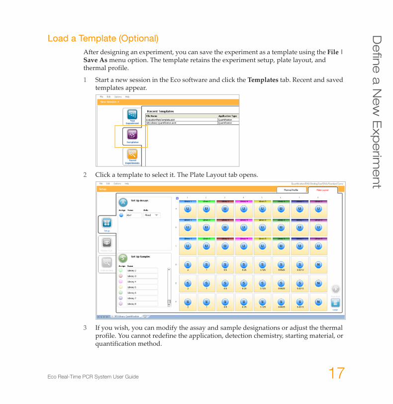
Load a Template (Optional)After designing an experiment, you can save the experiment as a template using the File | Save As menu option. The template retains the experiment setup, plate layout, and thermal profile.

1 Start a new session in the Eco software and click the Templates tab. Recent and saved templates appear.

2 Click a template to select it. The Plate Layout tab opens.

3 If you wish, you can modify the assay and sample designations or adjust the thermal profile. You cannot redefine the application, detection chemistry, starting material, or quantification method.

18 Part # 15017157 Rev E

Wo

rkflo

w Set Up the Plate Layout

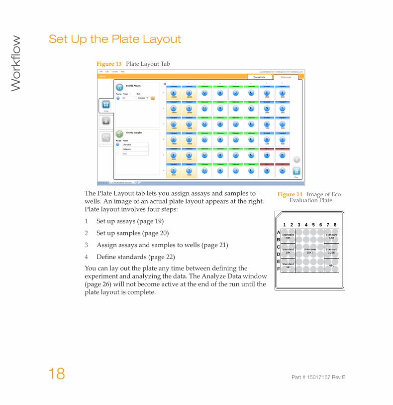
Figure 13 Plate Layout Tab

The Plate Layout tab lets you assign assays and samples to wells. An image of an actual plate layout appears at the right. Plate layout involves four steps:

1 Set up assays (page 19)

2 Set up samples (page 20)

3 Assign assays and samples to wells (page 21)

4 Define standards (page 22)

You can lay out the plate any time between defining the experiment and analyzing the data. The Analyze Data window (page 26) will not become active at the end of the run until the plate layout is complete.

1ABCDEF

2 3 4 5 6 7 8

Standard20K

Standard10K

Unknown[5K]

Standard5K

Standard2.5K

Standard1.25K

NTC

Figure 14 Image of Eco Evaluation Plate


Se

t Up

the

Pla

te L

ay

ou

t

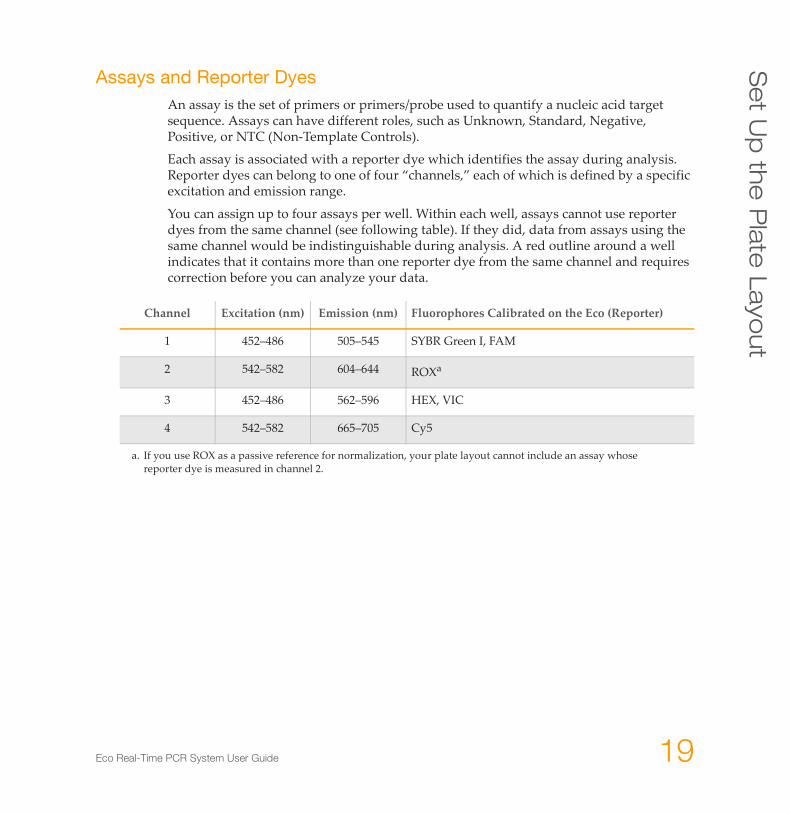
Assays and Reporter DyesAn assay is the set of primers or primers/probe used to quantify a nucleic acid target sequence. Assays can have different roles, such as Unknown, Standard, Negative, Positive, or NTC (Non-Template Controls).

Each assay is associated with a reporter dye which identifies the assay during analysis. Reporter dyes can belong to one of four “channels,” each of which is defined by a specific excitation and emission range.

You can assign up to four assays per well. Within each well, assays cannot use reporter dyes from the same channel (see following table). If they did, data from assays using the same channel would be indistinguishable during analysis. A red outline around a well indicates that it contains more than one reporter dye from the same channel and requires correction before you can analyze your data.

Channel Excitation (nm) Emission (nm) Fluorophores Calibrated on the Eco (Reporter)

1 452–486 505–545 SYBR Green I, FAM

2 542–582 604–644 ROXa

a. If you use ROX as a passive reference for normalization, your plate layout cannot include an assay whose reporter dye is measured in channel 2.

3 452–486 562–596 HEX, VIC

4 542–582 665–705 Cy5

20 Part # 15017157 Rev E

Wo

rkflo

w Set Up Assays

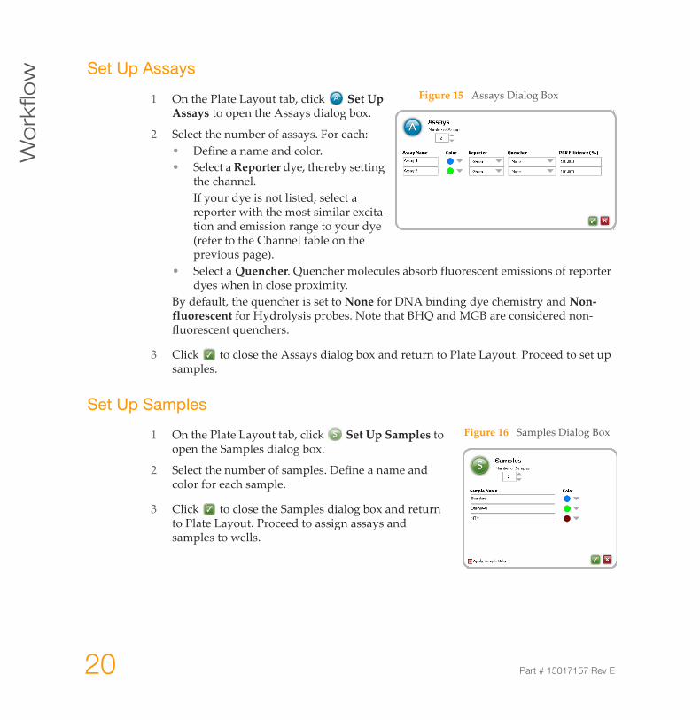
1 On the Plate Layout tab, click Set Up Assays to open the Assays dialog box.

2 Select the number of assays. For each:• Define a name and color.• Select a Reporter dye, thereby setting

the channel.If your dye is not listed, select a reporter with the most similar excita-tion and emission range to your dye (refer to the Channel table on the previous page).

• Select a Quencher. Quencher molecules absorb fluorescent emissions of reporter dyes when in close proximity.

By default, the quencher is set to None for DNA binding dye chemistry and Non-fluorescent for Hydrolysis probes. Note that BHQ and MGB are considered non-fluorescent quenchers.

3 Click to close the Assays dialog box and return to Plate Layout. Proceed to set up samples.

Set Up Samples

1 On the Plate Layout tab, click Set Up Samples to open the Samples dialog box.

2 Select the number of samples. Define a name and color for each sample.

3 Click to close the Samples dialog box and return to Plate Layout. Proceed to assign assays and samples to wells.

Figure 15 Assays Dialog Box

Figure 16 Samples Dialog Box


Se

t Up

the

Pla

te L

ay

ou

t

Assign Assays and Samples to Wells

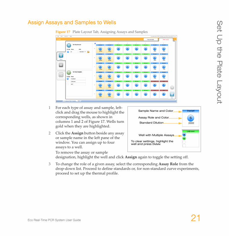
Figure 17 Plate Layout Tab, Assigning Assays and Samples

1 For each type of assay and sample, left-click and drag the mouse to highlight the corresponding wells, as shown in columns 1 and 2 of Figure 17. Wells turn gold when they are highlighted.

2 Click the Assign button beside any assay or sample name in the left pane of the window. You can assign up to four assays to a well.To remove the assay or sample designation, highlight the well and click Assign again to toggle the setting off.

3 To change the role of a given assay, select the corresponding Assay Role from the drop-down list. Proceed to define standards or, for non-standard curve experiments, proceed to set up the thermal profile.

Sample Name and Color

Assay Role and Color

Standard Dilution

Well with Multiple Assays

To clear settings, highlight the well and press Delete

22 Part # 15017157 Rev E

Wo

rkflo

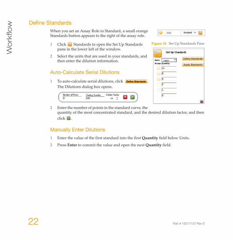
w Define StandardsWhen you set an Assay Role to Standard, a small orange Standards button appears to the right of the assay role.

1 Click Standards to open the Set Up Standards pane in the lower left of the window.

2 Select the units that are used in your standards, and then enter the dilution information.

Auto-Calculate Serial Dilutions

1 To auto-calculate serial dilutions, click .The Dilutions dialog box opens.

2 Enter the number of points in the standard curve, the quantity of the most concentrated standard, and the desired dilution factor, and then click .

Manually Enter Dilutions

1 Enter the value of the first standard into the first Quantity field below Units.

2 Press Enter to commit the value and open the next Quantity field.

Figure 18 Set Up Standards Pane


Se

t Up

the

Pla

te L

ay

ou

t

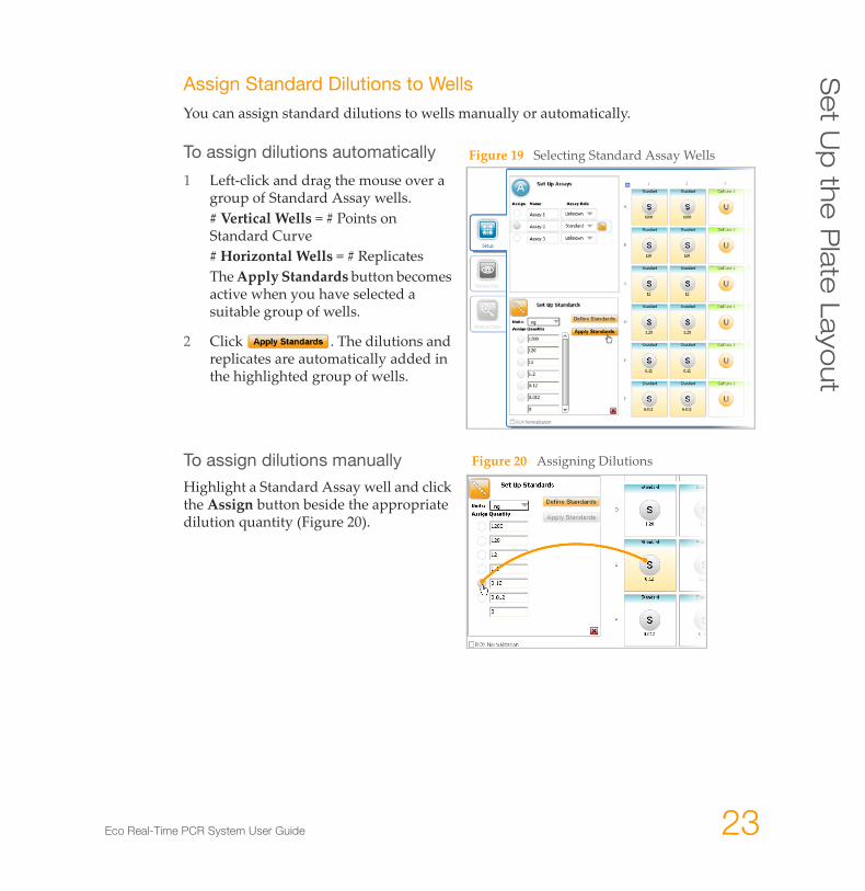
Assign Standard Dilutions to Wells

You can assign standard dilutions to wells manually or automatically.

To assign dilutions automatically

1 Left-click and drag the mouse over a group of Standard Assay wells.# Vertical Wells = # Points on Standard Curve# Horizontal Wells = # ReplicatesThe Apply Standards button becomes active when you have selected a suitable group of wells.

2 Click . The dilutions and replicates are automatically added in the highlighted group of wells.

To assign dilutions manually

Highlight a Standard Assay well and click the Assign button beside the appropriate dilution quantity (Figure 20).

Figure 19 Selecting Standard Assay Wells

Figure 20 Assigning Dilutions

24 Part # 15017157 Rev E

Wo

rkflo

w Set Up the Thermal Profile

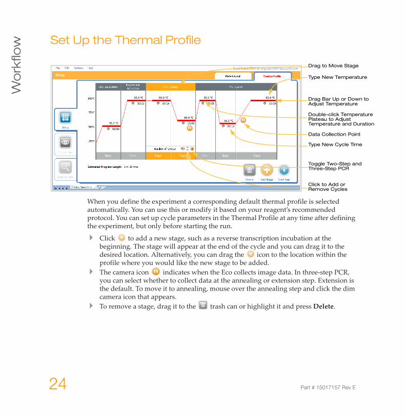
When you define the experiment a corresponding default thermal profile is selected automatically. You can use this or modify it based on your reagent’s recommended protocol. You can set up cycle parameters in the Thermal Profile at any time after defining the experiment, but only before starting the run.

Click to add a new stage, such as a reverse transcription incubation at the beginning. The stage will appear at the end of the cycle and you can drag it to the desired location. Alternatively, you can drag the icon to the location within the profile where you would like the new stage to be added.The camera icon indicates when the Eco collects image data. In three-step PCR, you can select whether to collect data at the annealing or extension step. Extension is the default. To move it to annealing, mouse over the annealing step and click the dim camera icon that appears.To remove a stage, drag it to the trash can or highlight it and press Delete.

Type New Cycle Time

Type New Temperature

Drag Bar Up or Down to Adjust Temperature

Toggle Two-Step and Three-Step PCR

Drag to Move Stage

Click to Add or Remove Cycles

Data Collection Point

Double-click Temperature Plateau to Adjust Temperature and Duration


Mo

nito

r Ru

n

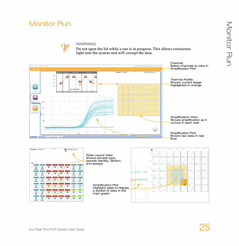
Monitor Run

WARNINGDo not open the lid while a run is in progress. This allows extraneous light into the system and will corrupt the data.

Thermal Profile:Shows current stage highlighted in orange

Amplification Plot:Shows raw data in real time

Amplification View: Shows amplification as it occurs in each well

Channel: Select channels to view in Amplification Plot

Amplification Plot:Highlight wells to display a subset of data in the main graph

Plate Layout View: Shows sample type, sample identity, dilution, and assays

26 Part # 15017157 Rev E

Wo

rkflo

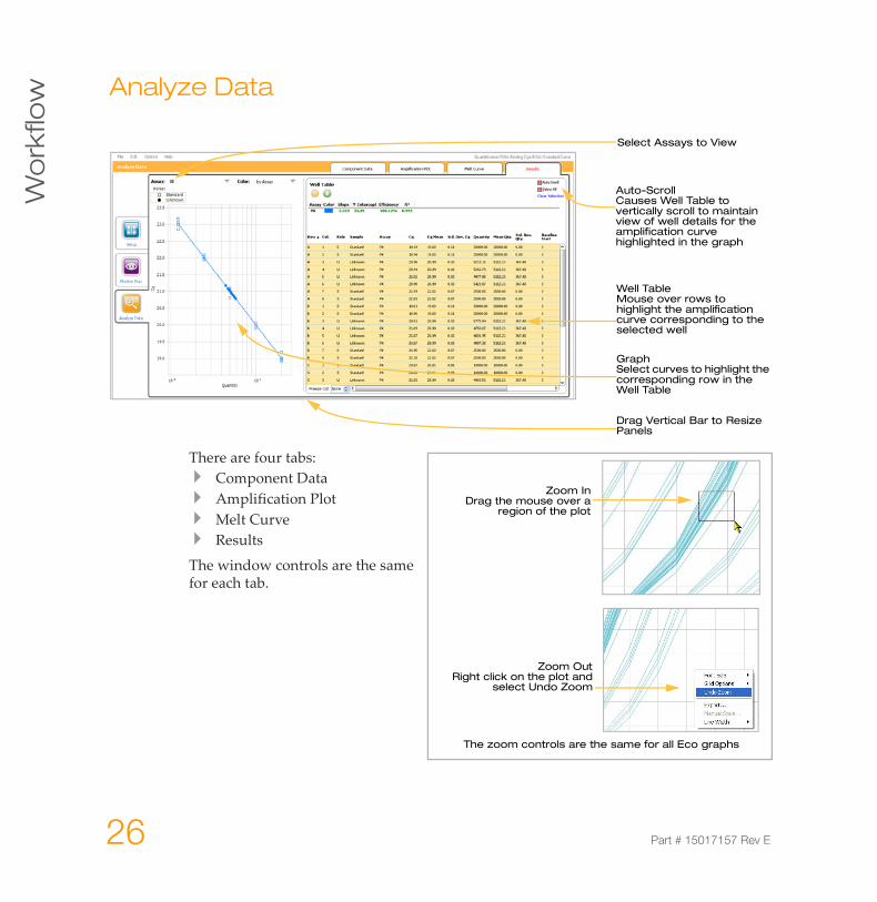
w Analyze Data

There are four tabs:Component DataAmplification PlotMelt CurveResults

The window controls are the same for each tab.

GraphSelect curves to highlight the corresponding row in the Well Table

Well TableMouse over rows to highlight the amplification curve corresponding to the selected well

Select Assays to View

Drag Vertical Bar to Resize Panels

Auto-ScrollCauses Well Table to vertically scroll to maintain view of well details for the amplification curve highlighted in the graph

Zoom OutRight click on the plot and

select Undo Zoom

The zoom controls are the same for all Eco graphs

Zoom InDrag the mouse over a

region of the plot


An

aly

ze

Da

ta

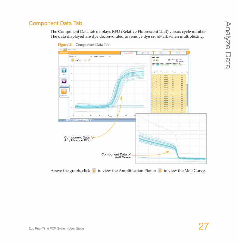
Component Data TabThe Component Data tab displays RFU (Relative Fluorescent Unit) versus cycle number. The data displayed are dye deconvoluted to remove dye cross-talk when multiplexing.

Figure 21 Component Data Tab

Above the graph, click to view the Amplification Plot or to view the Melt Curve.

Component Data for Amplification Plot

Component Data of Melt Curve

28 Part # 15017157 Rev E

Wo

rkflo

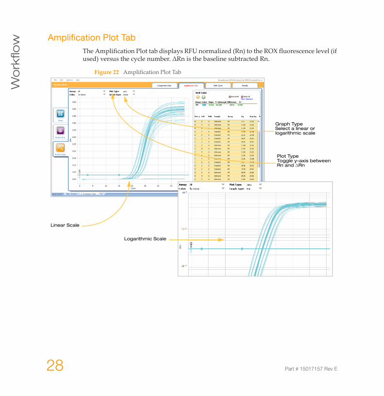
w Amplification Plot TabThe Amplification Plot tab displays RFU normalized (Rn) to the ROX fluorescence level (if used) versus the cycle number. ΔRn is the baseline subtracted Rn.

Figure 22 Amplification Plot Tab

Graph TypeSelect a linear or logarithmic scale

Plot TypeToggle y-axis between Rn and ΔRn

Linear Scale

Logarithmic Scale


An

aly

ze

Da

ta

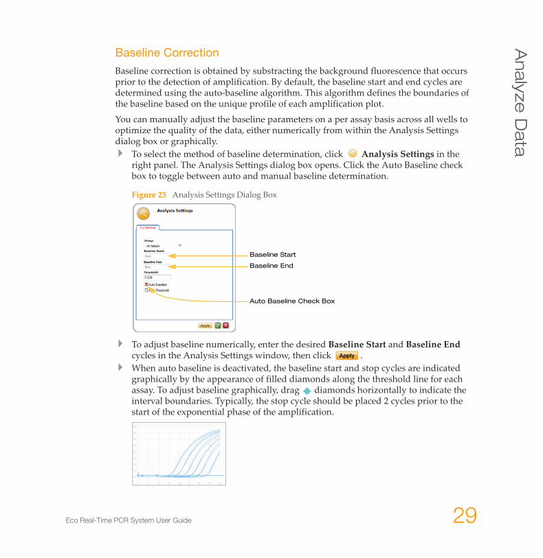
Baseline Correction

Baseline correction is obtained by substracting the background fluorescence that occurs prior to the detection of amplification. By default, the baseline start and end cycles are determined using the auto-baseline algorithm. This algorithm defines the boundaries of the baseline based on the unique profile of each amplification plot.

You can manually adjust the baseline parameters on a per assay basis across all wells to optimize the quality of the data, either numerically from within the Analysis Settings dialog box or graphically.

To select the method of baseline determination, click Analysis Settings in the right panel. The Analysis Settings dialog box opens. Click the Auto Baseline check box to toggle between auto and manual baseline determination.

Figure 23 Analysis Settings Dialog Box

To adjust baseline numerically, enter the desired Baseline Start and Baseline End cycles in the Analysis Settings window, then click .When auto baseline is deactivated, the baseline start and stop cycles are indicated graphically by the appearance of filled diamonds along the threshold line for each assay. To adjust baseline graphically, drag diamonds horizontally to indicate the interval boundaries. Typically, the stop cycle should be placed 2 cycles prior to the start of the exponential phase of the amplification.

Baseline Start

Baseline End

Auto Baseline Check Box

30 Part # 15017157 Rev E

Wo

rkflo

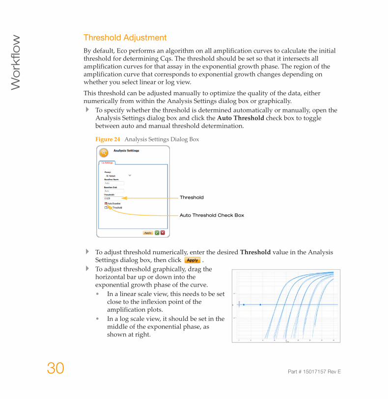
w Threshold Adjustment

By default, Eco performs an algorithm on all amplification curves to calculate the initial threshold for determining Cqs. The threshold should be set so that it intersects all amplification curves for that assay in the exponential growth phase. The region of the amplification curve that corresponds to exponential growth changes depending on whether you select linear or log view.

This threshold can be adjusted manually to optimize the quality of the data, either numerically from within the Analysis Settings dialog box or graphically.

To specify whether the threshold is determined automatically or manually, open the Analysis Settings dialog box and click the Auto Threshold check box to toggle between auto and manual threshold determination.

Figure 24 Analysis Settings Dialog Box

To adjust threshold numerically, enter the desired Threshold value in the Analysis Settings dialog box, then click .To adjust threshold graphically, drag the horizontal bar up or down into the exponential growth phase of the curve.• In a linear scale view, this needs to be set

close to the inflexion point of the amplification plots.

• In a log scale view, it should be set in the middle of the exponential phase, as shown at right.

Threshold

Auto Threshold Check Box


An

aly

ze

Da

ta

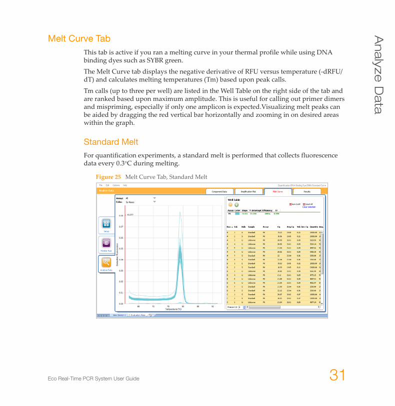
Melt Curve TabThis tab is active if you ran a melting curve in your thermal profile while using DNA binding dyes such as SYBR green.

The Melt Curve tab displays the negative derivative of RFU versus temperature (-dRFU/dT) and calculates melting temperatures (Tm) based upon peak calls.

Tm calls (up to three per well) are listed in the Well Table on the right side of the tab and are ranked based upon maximum amplitude. This is useful for calling out primer dimers and mispriming, especially if only one amplicon is expected.Visualizing melt peaks can be aided by dragging the red vertical bar horizontally and zooming in on desired areas within the graph.

Standard Melt

For quantification experiments, a standard melt is performed that collects fluorescence data every 0.3°C during melting.

Figure 25 Melt Curve Tab, Standard Melt

32 Part # 15017157 Rev E

Wo

rkflo

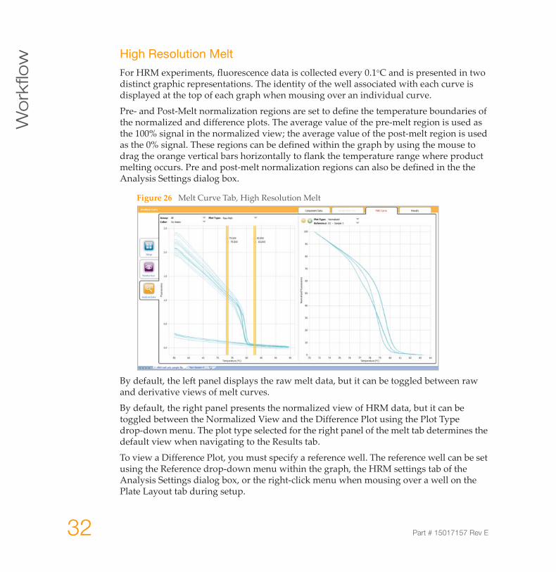
w High Resolution Melt

For HRM experiments, fluorescence data is collected every 0.1°C and is presented in two distinct graphic representations. The identity of the well associated with each curve is displayed at the top of each graph when mousing over an individual curve.

Pre- and Post-Melt normalization regions are set to define the temperature boundaries of the normalized and difference plots. The average value of the pre-melt region is used as the 100% signal in the normalized view; the average value of the post-melt region is used as the 0% signal. These regions can be defined within the graph by using the mouse to drag the orange vertical bars horizontally to flank the temperature range where product melting occurs. Pre and post-melt normalization regions can also be defined in the the Analysis Settings dialog box.

Figure 26 Melt Curve Tab, High Resolution Melt

By default, the left panel displays the raw melt data, but it can be toggled between raw and derivative views of melt curves.

By default, the right panel presents the normalized view of HRM data, but it can be toggled between the Normalized View and the Difference Plot using the Plot Type drop-down menu. The plot type selected for the right panel of the melt tab determines the default view when navigating to the Results tab.

To view a Difference Plot, you must specify a reference well. The reference well can be set using the Reference drop-down menu within the graph, the HRM settings tab of the Analysis Settings dialog box, or the right-click menu when mousing over a well on the Plate Layout tab during setup.


An

aly

ze

Da

ta

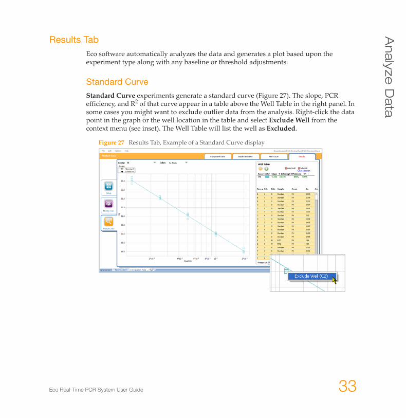
Results TabEco software automatically analyzes the data and generates a plot based upon the experiment type along with any baseline or threshold adjustments.

Standard Curve

Standard Curve experiments generate a standard curve (Figure 27). The slope, PCR efficiency, and R2 of that curve appear in a table above the Well Table in the right panel. In some cases you might want to exclude outlier data from the analysis. Right-click the data point in the graph or the well location in the table and select Exclude Well from the context menu (see inset). The Well Table will list the well as Excluded.

Figure 27 Results Tab, Example of a Standard Curve display

34 Part # 15017157 Rev E

Wo

rkflo

w Relative Quantification

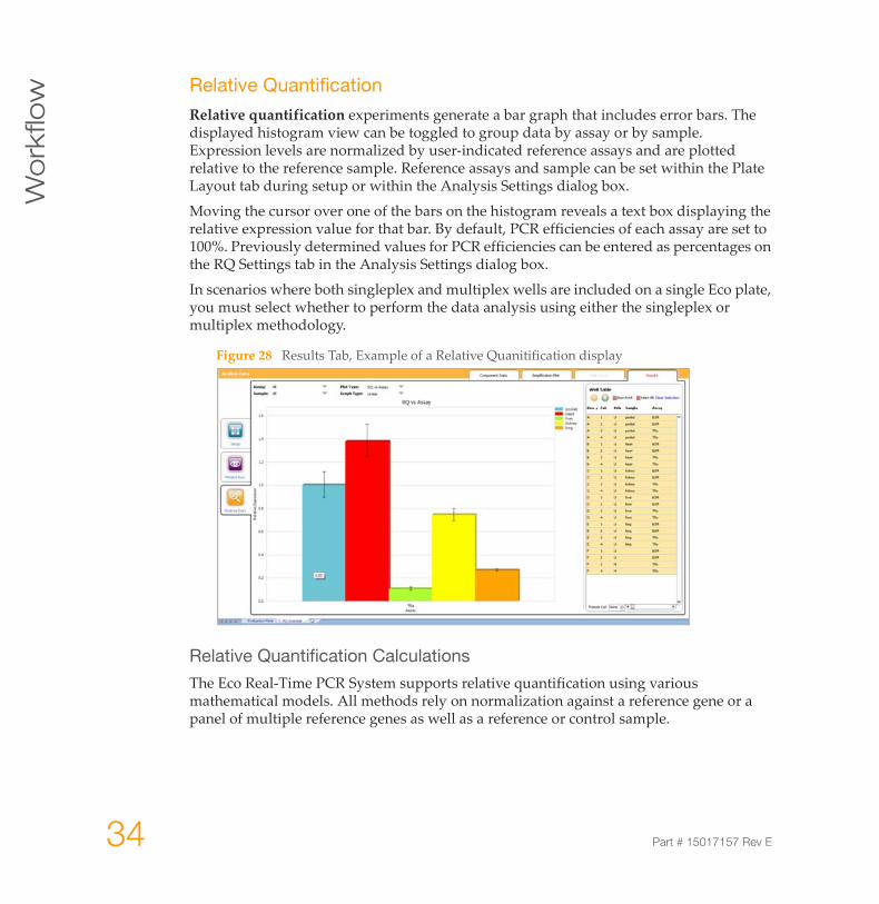
Relative quantification experiments generate a bar graph that includes error bars. The displayed histogram view can be toggled to group data by assay or by sample. Expression levels are normalized by user-indicated reference assays and are plotted relative to the reference sample. Reference assays and sample can be set within the Plate Layout tab during setup or within the Analysis Settings dialog box.

Moving the cursor over one of the bars on the histogram reveals a text box displaying the relative expression value for that bar. By default, PCR efficiencies of each assay are set to 100%. Previously determined values for PCR efficiencies can be entered as percentages on the RQ Settings tab in the Analysis Settings dialog box.

In scenarios where both singleplex and multiplex wells are included on a single Eco plate, you must select whether to perform the data analysis using either the singleplex or multiplex methodology.

Figure 28 Results Tab, Example of a Relative Quanitification display

Relative Quantification Calculations

The Eco Real-Time PCR System supports relative quantification using various mathematical models. All methods rely on normalization against a reference gene or a panel of multiple reference genes as well as a reference or control sample.


An

aly

ze

Da

ta

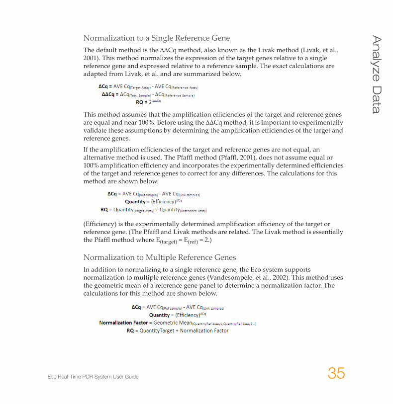
Normalization to a Single Reference GeneThe default method is the ΔΔCq method, also known as the Livak method (Livak, et al., 2001). This method normalizes the expression of the target genes relative to a single reference gene and expressed relative to a reference sample. The exact calculations are adapted from Livak, et al. and are summarized below.

This method assumes that the amplification efficiencies of the target and reference genes are equal and near 100%. Before using the ΔΔCq method, it is important to experimentally validate these assumptions by determining the amplification efficiencies of the target and reference genes.

If the amplification efficiencies of the target and reference genes are not equal, an alternative method is used. The Pfaffl method (Pfaffl, 2001), does not assume equal or 100% amplification efficiency and incorporates the experimentally determined efficiencies of the target and reference genes to correct for any differences. The calculations for this method are shown below.

(Efficiency) is the experimentally determined amplification efficiency of the target or reference gene. (The Pfaffl and Livak methods are related. The Livak method is essentially the Pfaffl method where E(target) = E(ref) = 2.)

Normalization to Multiple Reference GenesIn addition to normalizing to a single reference gene, the Eco system supports normalization to multiple reference genes (Vandesompele, et al., 2002). This method uses the geometric mean of a reference gene panel to determine a normalization factor. The calculations for this method are shown below.

36 Part # 15017157 Rev E

Wo

rkflo

w Allelic Discrimination

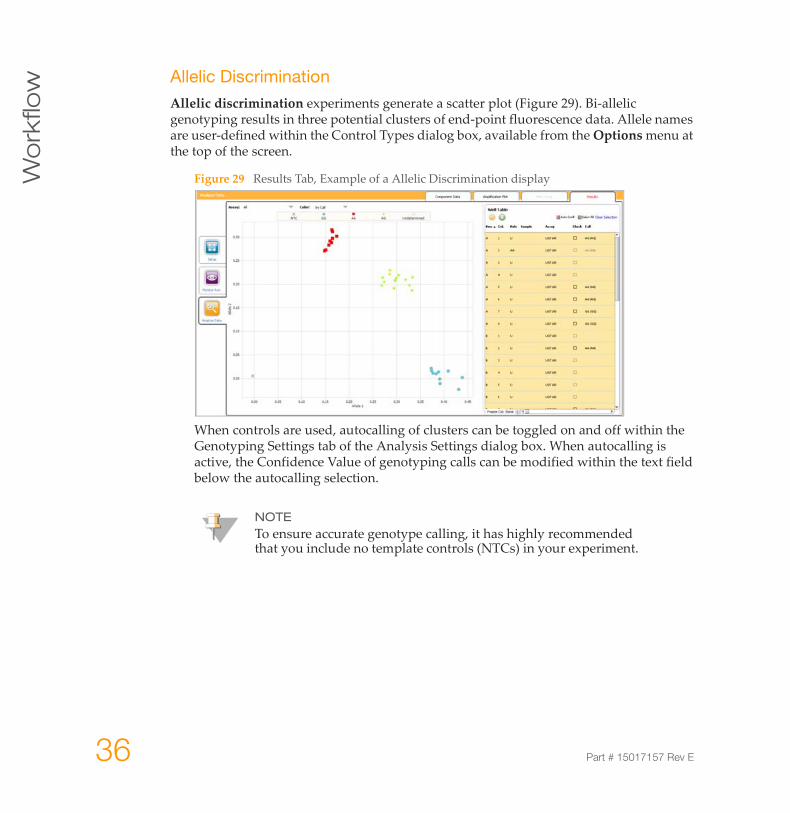
Allelic discrimination experiments generate a scatter plot (Figure 29). Bi-allelic genotyping results in three potential clusters of end-point fluorescence data. Allele names are user-defined within the Control Types dialog box, available from the Options menu at the top of the screen.

Figure 29 Results Tab, Example of a Allelic Discrimination display

When controls are used, autocalling of clusters can be toggled on and off within the Genotyping Settings tab of the Analysis Settings dialog box. When autocalling is active, the Confidence Value of genotyping calls can be modified within the text field below the autocalling selection.

NOTETo ensure accurate genotype calling, it has highly recommended that you include no template controls (NTCs) in your experiment.


An

aly

ze

Da

ta

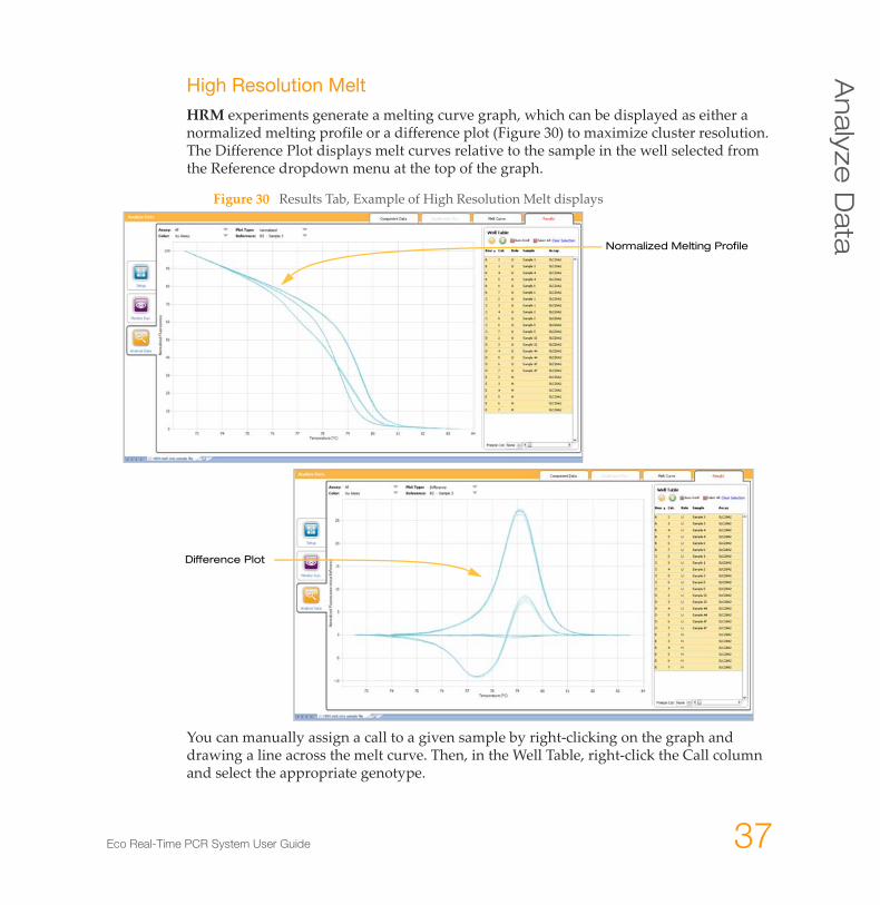
High Resolution Melt

HRM experiments generate a melting curve graph, which can be displayed as either a normalized melting profile or a difference plot (Figure 30) to maximize cluster resolution. The Difference Plot displays melt curves relative to the sample in the well selected from the Reference dropdown menu at the top of the graph.

Figure 30 Results Tab, Example of High Resolution Melt displays

You can manually assign a call to a given sample by right-clicking on the graph and drawing a line across the melt curve. Then, in the Well Table, right-click the Call column and select the appropriate genotype.

Normalized Melting Profile

Difference Plot

38 Part # 15017157 Rev E

Wo

rkflo

w Export Results and Data

Results, as well as other data, can be exported by clicking above the Well Table.

In the Export Options dialog box (shown left), select the desired file format and components to export, then click .


Ch

ap

ter 4

System Information

Components . . . . . . . . . . . . . . . . . . . . . . . . . . . . . . . . . . . . . . . . . . . . . . . . . . . . 40

Specifications and Environmental Requirements . . . . . . . . . . . . . . . . . . . . . . . . . 42

Symbols . . . . . . . . . . . . . . . . . . . . . . . . . . . . . . . . . . . . . . . . . . . . . . . . . . . . . . . 43

Electromagnetic Compatibility . . . . . . . . . . . . . . . . . . . . . . . . . . . . . . . . . . . . . . . 44

Cleaning And Maintenance . . . . . . . . . . . . . . . . . . . . . . . . . . . . . . . . . . . . . . . . . 45

Return Process . . . . . . . . . . . . . . . . . . . . . . . . . . . . . . . . . . . . . . . . . . . . . . . . . . 46

40 Part # 15017157 Rev E

Syste

m In

form

atio

n Components

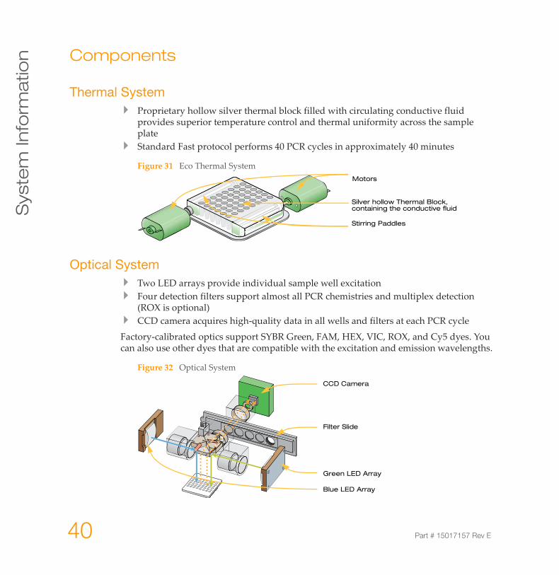
Thermal SystemProprietary hollow silver thermal block filled with circulating conductive fluid provides superior temperature control and thermal uniformity across the sample plateStandard Fast protocol performs 40 PCR cycles in approximately 40 minutes

Figure 31 Eco Thermal System

Optical SystemTwo LED arrays provide individual sample well excitationFour detection filters support almost all PCR chemistries and multiplex detection (ROX is optional)CCD camera acquires high-quality data in all wells and filters at each PCR cycle

Factory-calibrated optics support SYBR Green, FAM, HEX, VIC, ROX, and Cy5 dyes. You can also use other dyes that are compatible with the excitation and emission wavelengths.

Figure 32 Optical System

Motors

Stirring Paddles

Silver hollow Thermal Block, containing the conductive fluid

Blue LED Array

Filter Slide

CCD Camera

Green LED Array


Co

mp

on

en

ts

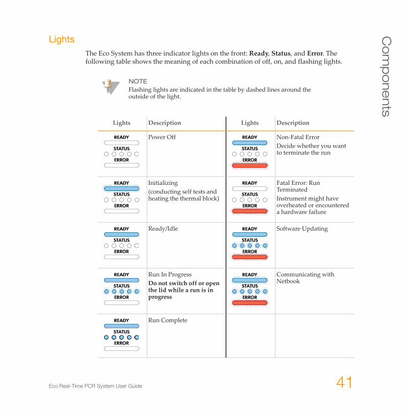
LightsThe Eco System has three indicator lights on the front: Ready, Status, and Error. The following table shows the meaning of each combination of off, on, and flashing lights.

NOTEFlashing lights are indicated in the table by dashed lines around the outside of the light.

Lights Description Lights Description

Power Off Non-Fatal ErrorDecide whether you want to terminate the run

Initializing (conducting self tests and heating the thermal block)

Fatal Error: Run TerminatedInstrument might have overheated or encountered a hardware failure

Ready/Idle Software Updating

Run In ProgressDo not switch off or open the lid while a run is in progress

Communicating with Netbook

Run Complete

42 Part # 15017157 Rev E

Syste

m In

form

atio

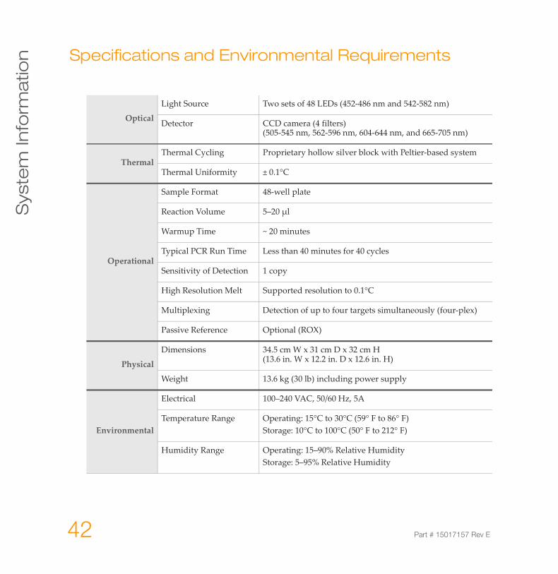
n Specifications and Environmental Requirements

Optical

Light Source Two sets of 48 LEDs (452-486 nm and 542-582 nm)

Detector CCD camera (4 filters) (505-545 nm, 562-596 nm, 604-644 nm, and 665-705 nm)

ThermalThermal Cycling Proprietary hollow silver block with Peltier-based system

Thermal Uniformity ± 0.1°C

Operational

Sample Format 48-well plate

Reaction Volume 5–20 µl

Warmup Time ~ 20 minutes

Typical PCR Run Time Less than 40 minutes for 40 cycles

Sensitivity of Detection 1 copy

High Resolution Melt Supported resolution to 0.1°C

Multiplexing Detection of up to four targets simultaneously (four-plex)

Passive Reference Optional (ROX)

Physical

Dimensions 34.5 cm W x 31 cm D x 32 cm H (13.6 in. W x 12.2 in. D x 12.6 in. H)

Weight 13.6 kg (30 lb) including power supply

Environmental

Electrical 100–240 VAC, 50/60 Hz, 5A

Temperature Range Operating: 15°C to 30°C (59° F to 86° F)Storage: 10°C to 100°C (50° F to 212° F)

Humidity Range Operating: 15–90% Relative HumidityStorage: 5–95% Relative Humidity


Sym

bo

ls

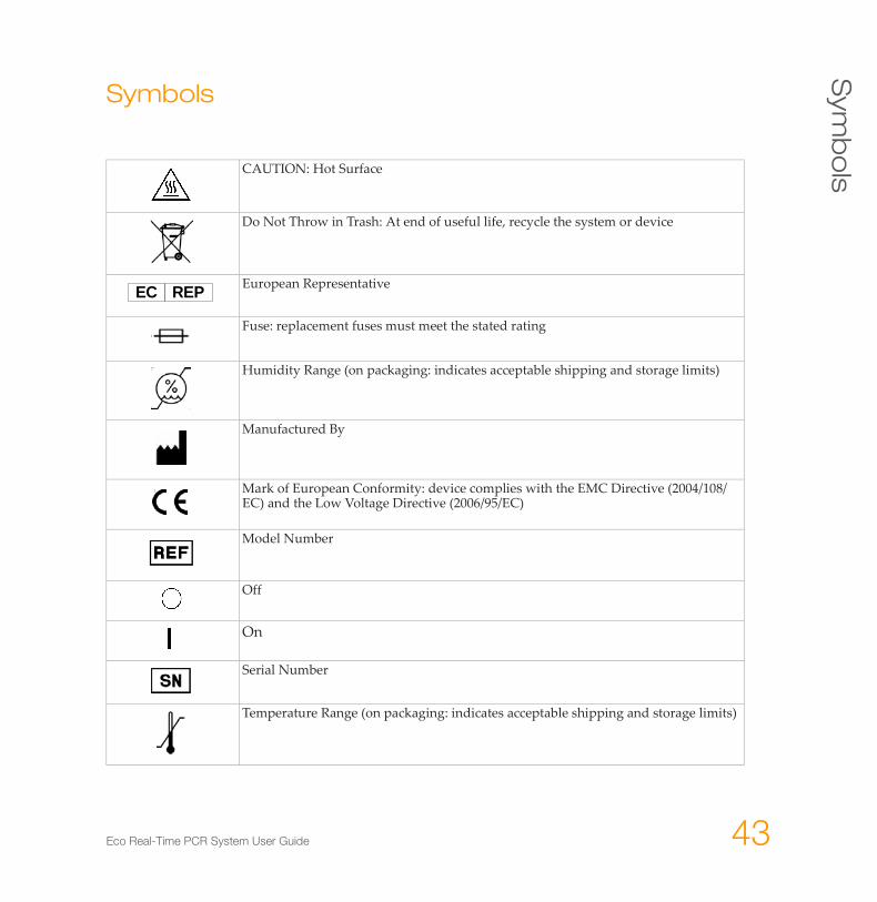
Symbols

CAUTION: Hot Surface

Do Not Throw in Trash: At end of useful life, recycle the system or device

European Representative

Fuse: replacement fuses must meet the stated rating

Humidity Range (on packaging: indicates acceptable shipping and storage limits)

Manufactured By

Mark of European Conformity: device complies with the EMC Directive (2004/108/EC) and the Low Voltage Directive (2006/95/EC)

Model Number

Off

On

Serial Number

Temperature Range (on packaging: indicates acceptable shipping and storage limits)

EC REP

44 Part # 15017157 Rev E

Syste

m In

form

atio

n Electromagnetic Compatibility

This equipment complies with the emission and immunity requirements described in IEC 61326-1:2005 and IEC 61326-2-6:2005. To confirm proper operation:

The electromagnetic environment should be evaluated prior to operation of the system.Do not use this system in close proximity to sources of strong electromagnetic radiation (e.g. unshielded intentional RF sources), as these may interfere with proper operation.If you notice any interference, discontinue using the system until all issues are resolved. Resolution may include moving cords from other equipment away from the system, plugging the system into an outlet on a different circuit from other equipment, or moving the system away from the other equipment. If you continue to have difficulties, contact Illumina.


Cle

an

ing

An

d M

ain

ten

an

ce

Cleaning And Maintenance

Clean the block and housing as needed, following these directions.

1 Turn the system off and allow the block to cool completely.

2 Using a lint-free cloth slightly dampened with clean water, gently wipe the surfaces of the equipment. If a stronger cleaning agent is needed, use a lint-free cloth slightly dampened with 95% isopropyl alcohol.

Follow these practices for proper maintenance of your Eco system.Every time you use the system, visually check it to confirm there is no obvious physical damage such as dents, frayed cords, or damaged levers. If you see any damage, discontinue use and contact Illumina Technical Support. Sign up for Illumina’s monthly Illuminotes newsletter, which tells you about new versions of systems or software, informational resources, and product discontinuations. Once a year, run a known test sample to confirm accurate analysis.

CAUTIONIf hazardous or biohazardous material is spilled onto or into the equipment, clean it immediately.

CAUTIONThe Eco system contains materials that may be hazardous to the environment if not disposed of properly. Be sure to dispose of materials according to all local, state/provincial, and national regulations.

46 Part # 15017157 Rev E

Syste

m In

form

atio

n Return Process

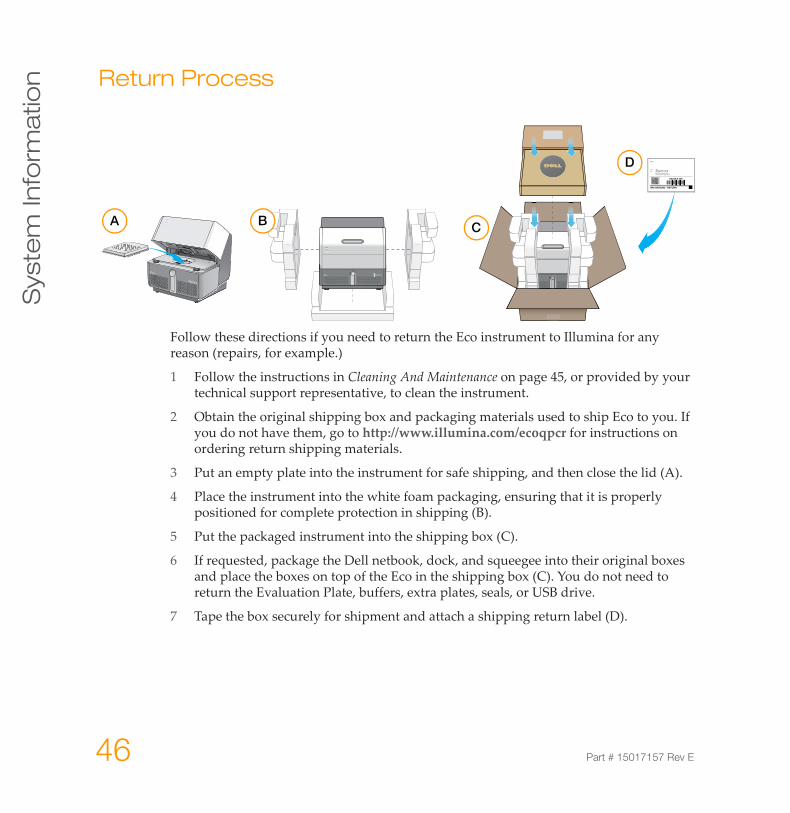
Follow these directions if you need to return the Eco instrument to Illumina for any reason (repairs, for example.)

1 Follow the instructions in Cleaning And Maintenance on page 45, or provided by your technical support representative, to clean the instrument.

2 Obtain the original shipping box and packaging materials used to ship Eco to you. If you do not have them, go to http://www.illumina.com/ecoqpcr for instructions on ordering return shipping materials.

3 Put an empty plate into the instrument for safe shipping, and then close the lid (A).

4 Place the instrument into the white foam packaging, ensuring that it is properly positioned for complete protection in shipping (B).

5 Put the packaged instrument into the shipping box (C).

6 If requested, package the Dell netbook, dock, and squeegee into their original boxes and place the boxes on top of the Eco in the shipping box (C). You do not need to return the Evaluation Plate, buffers, extra plates, seals, or USB drive.

7 Tape the box securely for shipment and attach a shipping return label (D).

A B C

D FROM:

SHIPTO:

SA240 9-100

UPS GROUND - RETURN

9865 Towne Centre DriveSan D iego, CA 92121 U .S.A.



Ch

ap

ter 5

Concepts

48 Part # 15017157 Rev E

Co

nc

ep

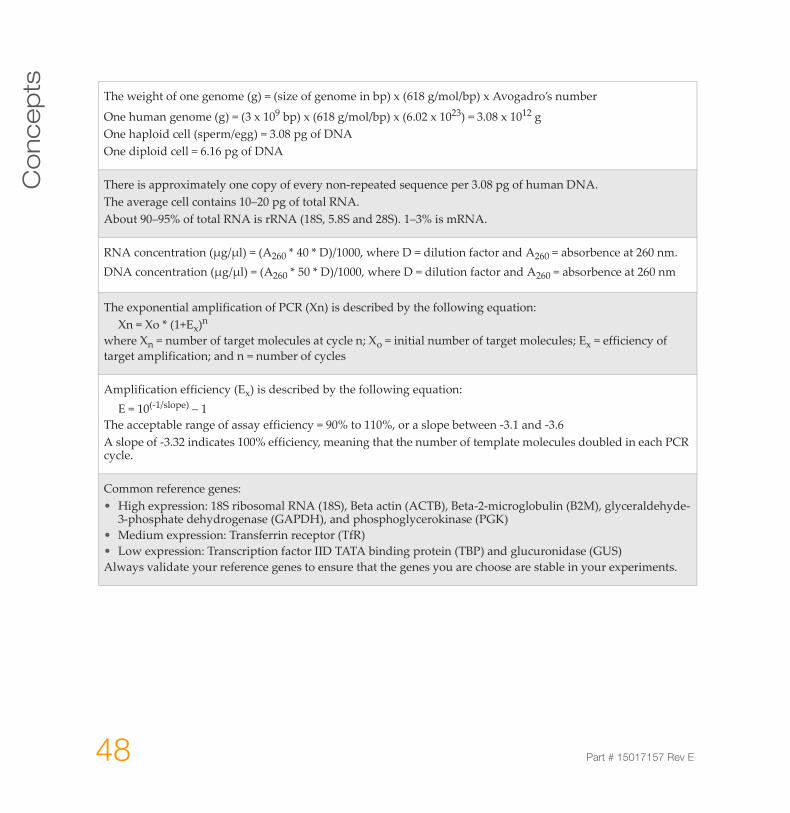
ts The weight of one genome (g) = (size of genome in bp) x (618 g/mol/bp) x Avogadro’s number

One human genome (g) = (3 x 109 bp) x (618 g/mol/bp) x (6.02 x 1023) = 3.08 x 1012 gOne haploid cell (sperm/egg) = 3.08 pg of DNAOne diploid cell = 6.16 pg of DNA

There is approximately one copy of every non-repeated sequence per 3.08 pg of human DNA.The average cell contains 10–20 pg of total RNA.About 90–95% of total RNA is rRNA (18S, 5.8S and 28S). 1–3% is mRNA.

RNA concentration (µg/µl) = (A260 * 40 * D)/1000, where D = dilution factor and A260 = absorbence at 260 nm.DNA concentration (µg/µl) = (A260 * 50 * D)/1000, where D = dilution factor and A260 = absorbence at 260 nm

The exponential amplification of PCR (Xn) is described by the following equation: Xn = Xo * (1+Ex)n

where Xn = number of target molecules at cycle n; Xo = initial number of target molecules; Ex = efficiency of target amplification; and n = number of cycles

Amplification efficiency (Ex) is described by the following equation: E = 10(-1/slope) – 1

The acceptable range of assay efficiency = 90% to 110%, or a slope between -3.1 and -3.6A slope of -3.32 indicates 100% efficiency, meaning that the number of template molecules doubled in each PCR cycle.

Common reference genes:• High expression: 18S ribosomal RNA (18S), Beta actin (ACTB), Beta-2-microglobulin (B2M), glyceraldehyde-

3-phosphate dehydrogenase (GAPDH), and phosphoglycerokinase (PGK)• Medium expression: Transferrin receptor (TfR)• Low expression: Transcription factor IID TATA binding protein (TBP) and glucuronidase (GUS)Always validate your reference genes to ensure that the genes you are choose are stable in your experiments.


Ch

ap

ter 6

Glossary

50 Part # 15017157 Rev E

Gloss

ary

Absolute Quantification—An assay that quantifies unknown samples by interpolating their quantities from a standard curve based on a serial dilution of a sample containing known concentration.

Allelic Discrimination—An assay that discriminates between two alleles (gene variants).

Amplicon—A fragment of DNA synthesized by a pair of primers during PCR.

Assay—The set of primers or primers/probe used to quantify an amplicon.

Baseline—The initial PCR cycles when little fluorescence signal is generated. This will be used to subtract the background.

Channel—The combination of excitation and emission spectra used to monitor amplification for a given assay.

Ct—Threshold Cycle. See Cq.

Cq—Quantification Cycle. The cycle number at which the fluorescent signal crosses the threshold. It is inversely correlated to the logarithm of the initial copy number.

Dark Quencher—A quencher without any native fluorescence. Black Hole Quencher (BHQ) dyes are an example.

Delta Rn (ΔRn)—The normalized Fluorescence of an amplification plot with background and ROX normalization dye correction.

Derivate Melt Curve—A plot of temperature (x axis) versus the derivate of fluorescence with respect to temperature (-dF/dT) (y axis). Used to analyze the Tm of an amplicon.

DNA Binding Dye—A dye that increases its fluorescence in the presence of double-stranded DNA.

dsDNA—Double-stranded DNA.

Dual-Labeled Hydrolysis Probe—See hydrolysis probe.

Dynamic Range—The range of template concentration over which accurate Cq values can be determined. Extrapolation is not recommended.

Efficiency—See Slope.

Endogenous Control—An RNA or DNA template that is naturally present in each sample.

End-Point Analysis—Qualitative analysis of PCR data at the end of PCR. Allelic discrimination assays (genotyping) are an example.

Exogenous Control—A RNA or DNA template that is spiked into each sample at a known concentration.


FAM (6-carboxy fluorescein)—The most commonly used reporter dye at the 5’ end of a Taqman probe.

Filter—Components used to limit the bandwidth or the excitation or emission energy to the next component of the optical path.

Fluorophore—The functional group of a molecule that absorbs energy at a specific wavelength and emits it back at a different wavelength.

Fluorescence—The immediate release of energy (a photon of light) as a result of an increase in the electronic state of a photon-containing molecule.

HEX—Carboxy-2’,4,4’,5’,7,7’-hexachlorofluorescein.

High Resolution Melt (HRM)—An enhancement of the traditional melt curve analysis which increases the detail and information captured.

Hybridization Probe—A probe that is not hydrolyzed by Taq polymerase. Hybridization probes can be used for melt curve analysis. Examples include Roche FRET and Molecular Beacons.

Hydrolysis Probe—A probe that is hydrolyzed by the 5’ endonuclease activity of Taq polymerase. Taqman probes are hydrolysis probes.

Internal Positive Control (IPC)—An exogenous control added to a multiplex qPCR assay to monitor the presence of inhibitors in the template.

JOE—Carboxy-4’,5’-dichloro-2’,7’ dimethoxyfluorescein.

LED—Light Emitting Diode. A light that is illuminated by the movement of electrons in a semiconductor material. LED lights do not have filaments that burn out and do not get very hot.

Linear View—A view of an amplification plot using linear dRn values (y-axis) versus PCR cycles (x-axis).

Log view—A view of an amplification plot using log dRn values (y-axis) versus PCR cycles (x-axis).

LUX Primer Set—A self-quenched fluorogenic primer and a corresponding unlabeled primer. When the primer is incorporated into DNA during PCR the fluorophore is de-quenched, leading to an increase in fluorescent signal.

Melt Curve—See Derivative Melt Curve.

Minor Groove Binders (MGBs)—dsDNA-binding agents typically attached to the 3’ end of Taqman probes. MGBs increase the Tm value of probes, thus leading to smaller probes.

52 Part # 15017157 Rev E

Gloss

ary

Molecular Beacons—Hairpin probes containing a sequence-specific loop region flanked by two inverted repeats. A quencher dye at one end of the molecule quenches the reported dye at the other end. Sequence-specific binding leads to hairpin unraveling and fluorescent signal generation.

Multiplexing—Simultaneous analysis of more than one template in the same reaction.

No Template Control (NTC)—An assay with all necessary components except the template.

Normalization—The use of control genes with a constant expression level to normalize the expression of other genes in templates of variable concentration and quality.

Passive Reference—A fluorescence dye such as ROX that the software uses as an internal reference to normalize the reporter signal during data analysis.

Peltier—Element used for heating and cooling in a qPCR machine.

Quencher—Molecule that absorbs fluorescence emission of a reporter dye when in close proximity. TAMRA and BHQ are quenchers.

R2 (Coefficient of Correlation)—The coefficient of correlation between measured Cq values and the DNA concentrations. It is a measure of how closely the plotted data points fit the standard curve. The closer to 1 the value, the better the fit. R2 is ideally > 0.99.

Reference—A passive dye or active signal used to normalize experimental results.

Reference Genes—Genes with a wide and constant level of expression. Typically used to normalize the expression of other genes. Examples of commonly used reference genes: 16S/18S, GAPDH, and b-actin.

Relative Quantification—An assay used to measure the expression of a target gene in one sample relative to another sample and normalized to a reference gene.

Reporter Dye—Fluorescent dye used to monitor amplicon accumulation. This can be a dsDNA binding dye or a dye attached to a probe. Each dye is associated with a certain channel.

Rn (Normalized Reporter Signal)—Reporter fluorescent signal divided by fluorescence of the passive reference dye.

ROX (carboxy-X-rhodamine)—The most commonly used passive reference dye.

Slope—The slope of a standard curve. It is a measure of assay efficiency. E = 10(-1/slope)-1, where a slope of -3.32 is equal to 100% efficiency (E) or an exact doubling of template molecules in each PCR cycle. Acceptable efficiencies range from -3.6 (90%) to -3.1 (110%). Overly high efficiencies indicate qPCR inhibition, usually due to contaminants in the sample. Overly low efficiencies typically indicate problems with the reaction mix concentration.


Standard—A serial dilution of a target of known concentration used as template to generate a standard curve.

Standard Curve—A plot of Cq values against the log of target amount. Used to determine an assay’s dynamic range, efficiency (slope), R2, and sensitivity (y-intercept).

Standard Deviation (SD)—The SD of replicate Cq measurements is a measure of the precision of the assay.

TaqMan Probe—See Hydrolysis Probe.

TAMRA—Tetramethyl-6-carboxyrhodamine. Commonly used as a quencher.

Target—The DNA or RNA sequence to be amplified.

Template—See Target. Template can also refer to a saved experiment that can be used as a model for new experiments in the software.

Threshold—A level set above the background signal generated during the early cycles of qPCR. When adjusted manually, it should be set in the middle of the exponential stage of qPCR.

TET—Carboxy-2’,4,7,7’-tetrachlorofluorescein.

Tm—The temperature at which 50% of dsDNA is single-stranded (melted).

Unknown—A sample containing an unknown amount of template.

Y-Intercept—In a standard curve, the value that crosses the y-axis at x = 1 (single copy target).

54 Part # 15017157 Rev E

Gloss

ary


Te

ch

nic

al A

ssis

tan

ce

Technical Assistance

For technical assistance, go to http://www.illumina.com/ecoqpcr.

MSDS

Material safety data sheets (MSDSs) are available on the Illumina website at http://www.illumina.com/msds.

Product Documentation

If you require additional product documentation, you can obtain PDFs from the Illumina website. Go to http://www.illumina.com/support/documentation.ilmn.

When you click on a link, you will be asked to log in to iCom. After you log in, you can view or save the PDF. To register for an iCom account, please visit https://icom.illumina.com/Account/Register.

http://www.illumina.com/msds

http://www.illumina.com/support/documentation.ilmn

https://icom.illumina.com/Account/Register


Illumina, Inc.

9885 Towne Centre Drive

San Diego, CA 92121-1975

+1.800.809.ILMN (4566)

+1.858.202.4566 (outside North America)

[email protected]

www.illumina.com

eco real-time system user guide - illumina...eco real-time pcr system user guide 3 real-time pcr...

Documents