).-.

tt

J .#

Applied EconometricTime Series

WALTER ENDERSloWaState University

Jox wILEY & soNs.mc.

PREFACE

'This book was borne out of fnlstration. After returning from aI1 cnjoyable and pro-ductivesabbatical at the University of California at San Diego, I bcgan expanding

7 the empirical content of my graduate-level classcs in macroecohomics and intelma-.

' M' ---

.

.;; tional t'inance.Students' interest surged as lhey began to understand th concunzntdevelopmcntof macroeconomic theot'y and time-series econometrcs. The differ-

' ence between Keynesins. monetarists. the rational expectations school. and thcir ability to explain me

71''

realbusiness cycle approach could best be understood by the. .

,i)empiricalregularities in the economy. Old-style macroeconomic mtdels were dis- 'carded becausc of their empirical inadequacies, not because of any logicltl inconsis- k,' '

'';!r7: ltencies. )

.'

,

''

.,

'

.

..

j

Iowa State University has a world-class Statistics Department, and most of our EE '

,

. ..j

,.

r,yeconomicsstudents take thrce of four statistics classes. Nevertheless. students' '' r ,

. q.. ).t ) rjbackgroundswere inadequate for the empirical portion of my courses. 1 needed to ttk '

. q .( k;. . ..;.,. !present A feasmable number of lectures on the topics covered in this book. M7 ;)'

t ?.7

frustrationwas that the journal articles were written for those already technically E5. ..)

. .

r',q'

,

proficientin time-selies' economctrics. The existing time-sdries texts were inade-.) kt'(

quate to the task. Some focsed on forecasting, others on theoretical econometric..j.issues, and still others on tecbniques that are intrequently used in the economics lit- i

erature. The idea for this text began as my class notes and use of handouts grew in- C. . l

ordinately.Finally, l began teaching a new coursc in applied time-series economet- E t.

)li CS . ( ' l

... j tMy orignal intent was to write a text on time-serits macroeconometrics. Fprtu- : rh ,

nately,my colleagues at Iowa State convinced me to broaden the focus; applied mi- ' ;' L

g.: r. - . ycroeconomistswere also cmbracing time-series methods. I decided to include ex- .,

;,q .:y

amplesdrawn from agricultural economics, international finance. and some of my i '. $.76. .)yk...j.gtt)work with Todd Sandlcr on thc study of transnational terrorism. You should find' .

: j.,.r

..

,. jjjt:.

:Ltc.,ytj.the examples in the text to provide a reasonable balance between macfoeconomic ' .

y',4

. .1.: .p.iri .-.;

and microeconomic applications. , 4 )! jk tThc text is intended for those with some background in fultiple regresslon '.

.

!rj :-j t

. jy. . .r.rjy.!:.jj(). y.) .analysis. I presulne the reder understands the assumptions underlying the tlse of .

.'L:).!.

.

,))t.. ?

ordina:yleast squarcs. X11of my students are familiar with the concepts of correla- l j ):y( :. . .y.;tiin and covariation', they also know how to tlse t-tests and Fltests within a regres- Sj. '$,?

j.

.t... , ,. c, . hi ;. .,7t..

.

-

.sion framework. I use terms juch as titean square drr/r, lgnycance fev'f. anq un- i ,l' ? k

. ..

tL'!)7# .#. jsbiased estimate without cxplaining thcir meaning. The last two chplers o the text 's. j'examine multiple time-jeries techniques. To work through these chapters, it is nec- 'it' 3. tf

. . . . . .). (.

),.ry jrf:..)jy

essae to know bow to solve a system of equations using mtrx algebra. Cbapter 1, ..s.y t tt. .

..

..

.. ! k.' tfentitled tDifference Equations. ' is the cornerstone of the text. In my cxperience.) . .t . '. i

. . .). ., . . 4 .. 1)

this material and a knowledge of regressipn are sufcient to bring students to th . );jT

. . ,.

. . yj.pointwhere they are able to read (he profesional jouimalsand to embark on a seri- ' rt lr.

tu dy ..

..

'

. l) . ., jous applird s

I bclicvc in tcaching by induction. Thc mcthotl is to take a simple example and.

build towards more general and more complicattld models and econometric proce- E

.(dures. Detailed examples of each procedure are provided. Each concludcs with a .

;

L'

'.

step-by-stepsummary of tlle stages typically employed in using that procedure. eae'

'

approach is one of learning by doing. A large number of solved problems are in- .

cluded in the body of each chapter. The Questionsand Exercises at the end of each'

chapter are especially important. ney have been designed to complement the ma- '

tedal in the text. In order to work through the excrcises, it is necessary to have ac-!

cess to a soware package such as RATS. SAS, SHAZAM, or TSP. Matrix pack-ages stlch as MARAB and GAUSS are not as convenient for univariate models.Packages such as MINITAB. SPSSX. and MICROFIT can perform many of theprocedurescovered in te exercises. You are encouraged to work through as manyof the examples and exercises as possible. The answers to all qnestions are con-tained in the lnstructor's Manual. Most of thc questions are answered in great de-tail. In addition, the Insructor's Manual contaias the data disk and the computerprograms that can be used to answer the end of chapter exerciscs. Programs areprovided for the most popular software packages.

In spite of a11 my efforts. some errors have undoubtedly crept into thc tcxt.Portions of the manuscript that are crystal clear to me, will surely be opaque to oth-ers. Towards this end, I plan to keep a list of corrections and clalifications. You canreceive a copy (ofwhat I hope is a short list) from my lnternet address ENDERS@IASTATE.EDU.

Many pcople made valuable suggestions for improving the manuscript. I am .grateful to my students who kept me challenge and were quick to point out errors.Pin Chung was especially helpful in carefully reading the many dras of the manu-script and ferreting out numerous mistakes. Selahattin Dibooglu at the Universityof Illinois at Carbondalc and Harvey Cutlcr at Colorado State University used por-tions of thc text in their own courses; thcir comments concerning the organization,style. and clarity of presentation are mucl) appreciated. My collengue Ban'y Falk

was more than willing to answcr my questions und make helpful suggestions. Hae-Shin Hwang, Texas A and M University; Paul D. McNelis, Georgetown University;H ad i Es ta l! a n , Un iv e rs ity o f I ll in o is ; M . Da n ie l W e s tbr ook , Ge o rge t o w nUniversity'. Beth Ingram. University of Iowa'. and Subhash C. Ray, University ofConnecticut al1 providcd insightful reviews of various stages of the manuscript.Julio Herrera and Nifacio Velasco, the

''food

gurus'' at the. Univers'ityof Valladolid.hclped me survive the final stages of proofreading. Most of all, I would like tothank my lovillg wife Linda for putting up with me while 1 was working on the text.

CHAPTER 1: Difference Equations1. Time-series Modeis2. Difference Equations and Their Solutions3. Solution by Iteration4. An Alternative Solution Methodology .

(.'

? .. . E.'

, .. '.

..2.

5. ne Cobweb Model6. Solving Homogeneous Diference Equations7. Finding Pmicular Solutions for Deterministic Processes8. The Method of Undetermined'cocfficients9 Lag Operators

l0. Forward-versus Backward-Looking SolutionsSummary and Conclusions

i 0 6 i 1 li lQuestons an xerc sesEndnotesAppendix l : Imaginary Roots and de Moivre's TheoremAppendix 2: Characteristic Roots in Higher-order Equations

CHAPTER 2: Stationary Time-series Models1. Stochastic Difference Equation Models2. ARMA Models

3. Stationarity4. Stationazity Restrictions for an

ARMAWV Model5. ne Autocorrelation Function6. ne Partial Autocorrelation Function7. Sample Autocorrelations of Stationa:y Series8. Box-lenkins Model Selection9. The Forccast Function

10. A Model of the WPl11. Seasonality

Summary and ConclusionsQuestionsand Exercises

EndnotesAppendix: Expected Values and Variance

CHAPTER 3: Modeling Economic Time Sries:t Trnds nd Volatility .

' 1.

'y 1. Economic Tim Series: The Stylized F@cts @i 2. ARCH Proc ssts

'

@t

. .

3. ARCH and GARCH Estqmatesof lnGation i494 . Estim :1l ing :) GARCH N1odel ( ) f'llle j'V1D1

J A 11 ! x :1!1)p1c 1525

.A GA 1)

-.

l 1 N1ol)tt 1 ( l' I-tisk 1566. Thc ARCH-M Model 158

, uaximumuikelihoouEstimation osoAucu anu ARcu-k. uo,il,. l6c8. Detenministic and Stochastic Trends : .

'

E' ): E ! 1669. Removing the Trend 176

l0. Are There Business Cycles? 18 1l 1. Stochastic Trends and Univariate Decompositions l85

Surllary and Conclusions 195Questionsand Exercises 196

Endnotes 204Appendix: Signl Extraction and Minimum Mcan Square Errors 206.

2112t222l22523323924325126026l265265

REFERENCES

AUTHORINDEX

SUBJECTINDEX

:T-i k..

,

)

X

35535636336537337738l3852933964O04O44054l0412

4l942042l

423

427

429

Chapter 1

DIFFERENCEEQUATIONS y' . . . ..

.... . ..

.. ).y)''.''.

' )..

he theory of difference equations underlies all the time-sefies methods employedin later chapters of this text. lt is fair to say that time-series econometrics is con-cerned with thc estimation of differcnce equatjons containing stochastic compo-nents.The traditional use of tim-series analysis was to forecast thu time path of avmiable.Uncovering the dynamic path of a series improves forecasts since the pre-dictablecomponents of the series can be extrapolated into the futurc. The growing

'

interest in economic dynamics has given a new emphasis to time-scries economst- jlics. Stochastic difference equations arise quire naturally from 'dynamic economic i .i

. .j.ymodels. Appropriately estimated equations can be used for the intepretation of lrlk

.

'

. .!'

.. .1

economicdata and for hypotesis testing.. r.?,'lyj

'I'he aims of this introductory chapter are to: , . t.7)t

.1'( ..g(

. yyk. .

. r.... . ... . tjrjj.: y.

l . Explain how stochastic difference equations can be used for forecasting and to 7Ei) 'q:i

,

. q, yillustrate how such equaiions can arise from familiar economic models. Tlie.

: 7 ,h

. j.' .-.'.

:'

.;(;;,.. .

-

. .

.

).'(j;l;,.j@,k.':.y'

'chapteris not meant to be a treatise on the theory:of differenc quations. Only #r'. (1 rty.

;. k. ! ;;

those techniques that are essential to the appropriate estimation f Iiner tim- '..:. t1,: ltik- 7)

L 'on single-eqation 'models: ''

''hEi' :X)$1tseries models are presented. This chapter focus s ( y. j:.

. .

..

. . y).. . jy ,.

multivariatemodels are considered in Chapters 5 and 6. :,. ; .y. ty tq

. k . . . y yjku)yj' $ '' difference equation. The solution will deter- -. i'z'2. Explain what it means to slve a . ).y j. jy; .., .. .. .

minewhether a variable has a stable or an explosive tifne path. A knwledge of r. :.. ' .

''

. ..

' ''m.

. ) f,..

xf.

the stability conditions is essential to undetstanding the recent innovaiions in.' F 7( '

). . . . . ..

q..J. :..;

. !..

time-selieseconometricsk' The contemporary time-series literature pays. special. . . t(.. (:;

')'

. . . ' . ) :.j..t

. ..

'y

attention to the issue ot- stationary versus nonstationary variablesr The stability.

'

t t:tt'.: .,

jt.jconditionsunderlie the conditions for statioarity. : ' ' ptk ); . ..

.

. ; :

., y , y N. ,.

3. Demonstrate how to fld the solution to a stochastic difference equation. There ' , )'jt.

. . :' - E' '; ''.

.. .

are Several differcnt techniques that can be used: each haj its own relative mer- ''','

. :' '

' its. A nuniber of examplej are presented to hlp yo uriderstand th: different ''

''

: 7 tjt.i. j

methods. Try to' work throuch each example carfully. For extra practice. you .

' '.,

should complete the exercises at the end of the chapter. '-.

(' 7 ''

. t .('

i

Dtfference f't?l/tJ/?'f.)tl'

1. TIME-SERIES MODELS

The task facing thc modern time-serics economtrtrician is to develop reasonablysimple models capable o forecasting, interpreting. nnd testing hypotheses conccrn-ing economic data. The challenge has grown ovcr time'. the original use of time-series analysis was primarily as an aid to forccastillg. As such. a methodology wasdevcloped to decompose a scfies into a trend. seasonal, cyclical, and an irregularcomponent.Uncovcring thc dynamic path of a st'ries improves forecast accuracysince each of the predictable components can 1,e extrapolated into the future.Suppose you observe the 50 data points show 11 il1 Figure 1. l and are interested inforecastingthc subsequent values. ausingthe time-series methods discussed inthe next several chapters. it is possible to decomplpse this series into the trend. sea-

Obsewed data

yrend

..-...- .- seasona l

1rre g u1a r Forecasts

Tme-series Models

sonal,and irregular components shown in the lower part of tbe figure. As you cansee, the trend changes the mean of the seres and the seasonal component imparts aregularcylical pattern with peaks occurring every 12 units ot-time. ln practice, thetrend and seasonal components will not be the simplistic detenninistic functionsshownin .the Ggure. With economic data, it is typical to t'indthat a series containsstochasticelements in the trend, seasonal, and irregular components. For the timebeing. it is wise to sidestep these complications so that the projection of the trendandseasonal components into periods 51 and beyond is straightfolvard.

Notice that the irregular component, whilc not having a well-dened pattem. issomewhat predictablc. lf you examine thc figure closcll'. you will see that thc posi-tivc and negative values occur in runs', the occurrence of a large value in any periodtends to be followed by another lftrge value. Short-run forcasts will make use ofthis positive correlation in the irregular component. Ovcr the entire span, however.the irregular component exhibits a te dency to revert to zero. As shown in thelower part of the figure, the projection ot- the irregular component past period 50rapidlyklecays toward zero.

'rhe

overall forecast, shown in the top part of the f'ig-ure, is the sum of each forecasted component.

The general methodology used to make such forecasts entails i'inding the 'tequa-

7, tion of motion'' driving a stochastic process and nsing that equation to predict sub-. )

,

j . jj- wg use tjjjs2: senuent outcomes. Let y, enote the value of a data point at neriod t.

:'

1'*

.

'''

'''

.

''t 'K ''

.

.

: . notation. the cxnmple in Figure 1.1

asFumed wa observed y! throtlgh yso. For l = 1( ! ; .

i.

y. : to 50. the enuations of motion used to construct components of the y, series are

:'.q'

;

' ''

.

!F Trend: Tt = 1 + 0. 1t!

Seasonal: St = 1.6

sintrn/z)Irregular: J, = 0.7 /,-1 + t

k'?'re Tr = value of the trend component in period t

.,= value of the seasonal component in t

I = the value of the irregular component in tt

6, = a pure random disturbance in f

Thus, the in-egular disturbance in l is 70% of the previous period's irregular distur-bance plus a random disturbnce tefm.

Each of these three equations is a type of diference equation. ln its most gen-erat form, a difference equation expresses the value of a variable as a function of itsown lagged values, time, and other variables. The trend and easonl tenns are bothfunctionsof time and the in-egular tenn is a function cf its own lagged valtle and

the stcchastic variable E,. The reason for introducing this set of equations is to makc

the point that tme-series economerics is ctpnccrzlct with lhe estimator of Jt/-/r-

enceecyltcrfapTs contakning slochastic co??lponcnrj. Thc tim-seris econometrician

mayestimate the propcrties of a single series or a vcctor containin: mahyin'terde-'

.endent series. Both univariate and multivariate torecastingmetbods are prejented. Pin tbe text. Chapter 2 shows how to estimate the irrejular part of a series. The firsthalfof Chapter 3 considers estimating the variance when the dta exhibit je'Iiods o

' 4

I=)',)

lrt l

1 '.

DIfJerence f'l/t:f I'o?T.y

volatility and tranquility. Estimation of the trend is considered in thc last half ofChapter 3 and in Chapter 4. Chaptcr 4 pays particular attcntion to the issue ofwhether the trend is deterministic or stochastic. Chapter 5 discusses the propertiesof a vector of stochastic difference equations nnd Chapter 6 is conccrned with theestimatiopof trends in a multivariate model.

Although forecasting was the mainstay of time-series analysis. the growing im-portance of economic dynamics has gencrated ncw uses for time-series analysis.Many economic theories have natural reprcselllations as stochastic diffcrcnce equa-tions. Moreover, many of these models have tcstablc implications concerning thetime path of a key economic valiable. Considcr the following three examples.

l . The Random Walk Hypothesis: In its simp+st form, the random walk model 'suggests that day-to-day changes in the plice of a stock should have a meanvalueof zcro. Aer all, if it is known that a capital gain can bc made by buyinga shnre on day J and sclling it for an cxpccted proflt hhc very next day. efficientspeculationwill drive up the current price. Similarly, no one will want to hold astock if it is expected to depreciate. Formall. tl4e model asserts that the price of

a stock should exolve according to the stochastic difference equation:

)' l=

v'l + f.,+I14'

y:., = 6,+ ,

wlere y, = the price of. a share of stock on day

6,+1= a random disturbance tcrm that llas an expected value of zero

N()w consider tLe more general stochastic diflrel:ce equation:

AA',+l= W)+ tlt11'/ + Er+ 1

The random wnlk llypothesis requires thc tcstable restriction cto = aj = 0.Rcjccting this rcstriction is cquivalent to rcjccting thc thcory. Givcn thc infor-nlation availablc in period , the theory also rcquires that the mean of 6.,+1 beequal to zero', evidence that 6.,.1 is predictable inval kdates the random'walk hy-pothesis.Again, the appropriate estimnlion o a singlc-equation model is consid-ered in Chapters 2 through 4.

2. Reduced Forms and Structural Equations: Oftcn. it is useful to collapse asystem of difference equations into separate single-equation models. To' illus-trate the key issues involved. consider a stochastic version of Samuelson's(l 939) classic model:

> T''!

';

)1

l.3

) T-11r*.kjl.;.

: !**1 !1

.!

y:= cr + it

c, = ayf- l + ecr O < (y, < 1il= fstcf- cr- I ) + E,., f.l> 0

wherey,, c,, and I', denote real GNP, consumption, and investment in time period

t, respetively. ln this Keynesian model, y,, c,. and i, are endogenous valiables.

The previous peliod's GNP and consumption. yt-l and c,-,, are called predeter-minedor lagged endogehous variables. The terms E, and 6,., are zero mean ran-dom disturbances for consumption and investment and the coefticients c, and ;$are parameters to be estimated.

The first equaton equates aggregate output (GNP) with the sum of consump-tion and investment spending. The sccond cquation asserts that conspmptiol)

spendingis proportional to the previous period's income plus a random distr-bance term. The third tquatioil illustrates the accclcrator principle. Investmentspendingis proportional to thi chnge in consumption; (he idea is tllat growth inconsumptionnecessitates new investment spenzing-E ne error tenns Ec, and Eg,

represent the poflions of consumption and investmnt'not

explained by the be-havioralequations of the model.

Equation (1.3)is a structural equation since ii expresses tc endogcnousl

variable i: as being dcpendent ori t current realiz tion of another endogenousvariableG. A reduced-fonn equation is one expressing the value of a variable

in tenns of its own lggs. lags of other endogtnous variables, current and past1 s of exogenous variables and disturbace tens. As formulated, the con-va ue ,

; sumption function is already in reduced fonn; cufrent consumption depends( j b tennonly on lagged income and th current value of the stochastic d stur ance

Ecr Investment is not in reduced form since lt depends on current period con-sumption.

To derive a reduced-fonn equation for investment, substitute (1.2)into the inr

vestmentequation to obtain

it= f'5(a.y,-,+ ec, - c?-l) + ei:

= txl3yl.-, - pcr-l+ f'JEc? + E,.,

Notice that the reduced-fonn equation for investment is not unique. You canlag'(1.2)one period to obtain c,-) = co-c + Ec,-l. Using this expression, we canalso write the reduced-fonn investment equation as

it= t:/,f5.F1-:- 2(t7..J,/-2 + Ecr-l) + Ec, + Ef?

= (7.fJ(.),,-!- y,-c) + 0(Ec, - ecr-l) + it

Similarly, a reduced-form equation for GNP can be obtainrd by substituting

( 1.2)

and (1.4)

into (1 . 1):

y,= ayr-, + Ec, + l3t-yl-.,- yr-z) + p(Ecr - Ec,-,) + Ef,

= c,41 + jJ)y,..j= ajx-.a + (1 + j)Ew + ir- j'Je.w..l ( l

.!)

Equation (1.5) is a univariate reduced-orm tqation; y, is expressed solelyas a function of its own lags anl disturbance terms. A univariate model is partic-ularly useful for forecastinj since it enasles you to jredict'a series based iolely

Tme-seres Models

lr-1;

D ./J relce E lztl/lo?l' ' ' '

l e q

on its own currcnt and past realizations. 11is possible to estmate (1.5) using theunivariate time-series techniques explained il1Chapters 2 through 4. Once youobtain estimates ot- (x and I),it is straightfonvard to use the observed values of ylthrough y, to predlct all future values in the series (i.., y,+!, y/.c, ... ).

Chapter 5 considers the estimation of multivariate models when al1 variablesCtI'c trcatctl as joiIltly cntlogenous. The chapl cr also discusses the restrictionsnccded to recovel' ( i .c.. idcllti fy) thtt strtlcttl l':t1 model from the estimated rc-duccd-forfn model.

Error Correction: Forward and Spot Pricts. Certain commodities antl finan-cial instruments can be bought nd sold on thc spot market for immediate deliv-el'yor for delive:y at some specified future date. For example. suppose that the'pfice of a particular foreign currency on the spot market is J, dollars and theprice of the currency for delivery one-pefiod into the future is S dollars. Now,consider :t speculator who purchased fonvard currcncy nt !he price dollnrs perunit. At tbe beginning of period t + 1, hc speculator receives the currency andpays.j dollars per unt received. Since spot forcign exchange can be sold at stwj,the spcculator can earn a prot'it (orloss) of .,.j

-f

per unt transactek..

The unbinsed forward rate (UFR) hypothesis asserts that expected profitsfrom such spcculative behavior should be zero. Formally. the hypothesis positsthe following relationship between fonvard and spot exchange rates:

u ! =J?+ E,.,

where E,.) has a mean value of zero from the Tlerspective of time period t.ln (1

.6).

the ronvardratc in t is an unbiascd estimate of the spot rate in t + 1.Thus. suppose you collccted data on the two rates and estimated the regression:

sl..t= Czo + Czl./i + E?+,

If you werc able to concludc thal co = 0s a! = J and lhe regrcssion residuals

6.,+1have a mean valuc of zcro from the pcrspcctive of time period t. the UFRhypothcsis could be maintained.

The spot and forward markets are said to bc il1A'long-rtln cquflibrium'' when

q,+, = 0. Nvhencvcr &,+) turns ont to dif-ferfrom. some sort of adjustment mustoccur to restorc the equiliblium in thc stlbsequent period. Consider the adjust-

m (')11t g)I-OCCSr;:

Dtjerence f'llalEfp/l.$' fznd Their Solutions

tion model since the movement of the variables in any pcriod is related to thcpreviousperiod's gap from long-run equilibrium. If the spot rate .,.I turns out toequal the forward ratef. ( l

.7)

and (1.8)

state that the spot and folavard rates are' h d lf there is a positive gap between the spot andexpected to remain unc ange .

fonkard rates so that st-vt-./)

> 0, ( l.7)

and (1.8)

lead to the prediction that the

spot rate wil! fatl and the forward ratc will rise.

DIFFERENCE EQUATIONS AND THEIR SOLUTIONS

Although many of the idcas in the previous section wcre probably familiar to you.it is necessary to fonnalie some of the concepts used. lh this section. we will ex-amine the type of difference equation used in econometric analysis and make ex-plicitwhat it means to e'solve'' such equations. To begin our examination of diffes

ence quations. consider the function y =X1).If we evaluate the function when theindependentvariable t takes on the specific value l*, we get a specc value for the

dependentvaliable called y,.. Formally, y,. = jt*l. lf we use this same notation,

y,.+, represents the value of y when t takes on the specitsc value t* + h. The firstdifferenceof y is defined to be the value of the function when evaluated at t =

1*+ h mnus the value of the funtion evaluated at f*: '

tsyts..h EX XJ* + /l) -XJ*)O 9t.+h - yt.

Differential calculus allows the change in the independent variable (i.e., the termh) to approach zero. Since most economic data are collected ver disrete periods. 'however,it is more useful to allow the length of the tme period to be greater than

zero. Usng difference equations. we normalize units so that h represents a unit

change in' t (i.e., = 1) and considcr the sequence of equally spaced vzlues or the

independentvariable. Without any loss of generality, we can always drop the asler-iskon J*. We can then form the first differences:

32J c:z y() - / ..- J) & y .-. yj-yy I

A)',+l=.It + '+, 'jy' :

j uu .Apg+a=ht+ 2) -X! + ) j't-z Fl+l

%t+z= st.. - a(.,+.$

-./;)

+ E,?+a t: > 0)'t+l

=./;+ 7(5.,+.1-.J,)+ 6.?i., ;$> 0

whcre E,.a and 6y,.1 both have a mean valuc ('f zel k) from the perspective of timeperiod t + 1 and 1. respectively.

Equations (1.7)and (1.8) illustrale the type of silnultaneous adjustment mech-anlsm considcred in Chapter 6. This dynamic model is called an error-correc- .

Often, it will be convenient to exprcss the entire sequence of values (... )'t.n . y?-,.

y,. y?.! ? yr.ez.... ) as fy,). We can thcn refer to any one particulnr value in the se-

quence as y,. Unless specified, the index t runs from -e,o to +e.o. In time-series .

econometric models. we will use t to rcpresertttme'' and h the length of a time pr- ''

. .'''

. .

riod. Thus, y, and y,.1 might rcpresent the realizations of the (y;j sequcnce. n the .

first and second quarters of 1995. rcspcctively.

ln thc same way, we can form the second diffrenc as the chang in the firstdi ffkrcnce. Considi r '

Digerettce kuclrln.

A2y, H A()',) = A(.,y,- yt- I) = (A',- y,- I) - (-5.,-)- .v,-2) = yt - 2y,-1+ y,-.cA2v,+

Ir'B (AA',..1) = (.,?+r

- y,) = (.vtvt-

.y,)

- ('.vt-.v,-

I) = A'/+1- 2y, + yt-.t

Thc ?2th diffrrencc (c) is dfzfincdanalogotlsly. At lllis point, we risk taking thelheory of differcnce equatons too far. As you wi1l sce. (he need to use second dif-fcrences.rarelyarises in timc-series analysis. lt is safe to say that third- and higher-order differences are. never used in applied work.

Since this text cons iders lincar time-series mc (llotlrk, it is possible to examineonly the special case of an rlth-order linear differencc etluation with constant coeffi-cients, Thc form rtlrthis special type of di f'fcrcncc cqualion is given by

The order of the difference equation is given by the value of n. The equation is lin-ear because a1l values of the dependent variabkc are raised to the first power.Economic theory may dictate instances in which the various ai are functions e 'variables within the economy. However. as long a's thcy do not depcnd on any ofthe values of y, or -vs

we can regard tlem as paramcters. The tem xt is called theforcing process. The form of the forcing process cktn be very general',x, can be anyfunctionor time, cufrent and lagged values of othcs' variables, and/or stochastic dis-turbances.By appropriate cloice of the forcing prbcess. we can obtain a wide vari-

ety of important macroeconomic models. Rcexamine Equation (1.5),

the reducedfonmequation for GNP. This equation is a second-tlrder difference equation since y,depends on yr-c. The forcing process is the expression (1 + j)Ec, + Ef, - pEc?-I. YOu

will note that (1,5)

has no intercept term corresponding to the expression av in( ) . 10).

An important special case for the (.'r,)scquence is

...

..'

..

t'

' ' '.'

whcre thc k'Jfare constants (someqf which can cqual zcl'kll and the individual elc-

ments of tbe sequence (e,) are not functions of the yt. At ths point, it is useful toallow the (E,Jsequencc to be nothing more than a sequcnce of unspecified exoge-nous variables. For example, let (6.Jbe a random cn'or term and set fsa= l and f5l=f'Ja= ... = 0, then Equation ( i

.1

0) bcconlcs the auttregression equation:

Let n = l , ao = 0, and ak = 1 tcl obtain tllc random wktlk Iltldel. Notice that Equation(1. 10) can be . vritten in terms of the difference operato) (A). Subtracting y,-l from( 1. 1O). Nve obtt Lin

.: :'.'' E.. .'.'

.:.. .

t'

.'

k diisng yL:;.F(aj - l)?w.eg44

xttitk, ELy = t'a + YA'r-1+ aiyt-i + A'tf ..'

i= 2

Clearly, Equation (1.1l ) is just a moditied version of (1. l0).A solution to a difference equation expresses the value of y, as a function of the

) lues of the (y,) se-elementsof the (m) sequence and t (andpossibly some g vcn va

quence called initial conditions). Examining (1.1

1) makes it clear that there is a

stronganalogy to integral calculus when the problem is to find a primitivc ftlnctionfrom a given derivative. We seek to nd the ptimitive function

./(f)

given an equa-tion expressed in the fonn of (l

.10)

or (1.11). Notice that a solution is a functionrather than a number. The key property of a solution is tat it satisfies the differ-

ence equation for all pennissible values of l and (.x,J. Thus, the substitution of a so-lution into the difference equation must result in an identity, For example, considerthe simple difference equation Ay,'= 2.(ory, = y,-1 + 2). You can easily' kerify that asolutionto this difference equation is yt = 2/ + c, where 'c is any arbitrary constant.By definition, if 2t + c is a solution, it must hold for a11permissible values of t.Thus for peliod t - 1,yr-, = 2(I - 1) + c. Now substitute the solution into the differ-

encc equation to fonn

2J + c M 2(J - 1) + c + 2

It is straightforward to carry out the algebra and verify tat ( l.12)

is an identity.This simple example also illustrates that the solution to a difference equation need

not be unique', there is a solution for any arbitrary value of c.Another useful example is provitled by the irregul:tr tenm shown in Figure 1

.1

;

11that the equation for this expression is It = 0.7/,-, + e,.rou

can vertfy that therecasolutionto this first-ordcr equation is

''N iIt = (0.7) El-,f

/=0

: Since' ( l.13)

holds for a1l time periods, the value ot- the ifregular cmponent iny ,

.

. ; .

' ( - l is tivenby :': ; E! . ,(J. j .'

, .:.j'. .i)

-'

7-

i .2J = (0.7) e I-f

:( ( l . l4)1- l 1- ; ..

i=0 ''

.

Dilje re n ce I:-f.pIz (1 l io n .

Thc two sidcs of (1.1

5) are identical-, this proves that (1 . 13) is a solution to thefirst-orcter stochastic difference equation lt = 0.7/,-1 + E,. Bc aware of the distinctionbetwcen reduced-form equations and solutions. Since /, = 0.7J,-) + E, holds for a1lvalucs of J, it follows that lt-, = 0.7-c + E,-1 . Combining thcse two equations yields

l = 0.7(0.71 + E 1) + E, ' !,. t $

. ..''.. t t -- ;! f-- .

= 0.49/,-a + 0.7E,-) + e, : 'q :, E.

E:' . .. .. .. ... .. . .

' . '. . ' ' . t..)

Equation (1.16)

is a reduced-form cquation sillce it expresses h in terms of itsown lags nnd distnrbance tenns. Howcver. (1. 1(?) does not qualify as a solutionsincc it contains the ''unknown'' valuc of It-z. To qualify as a solution. (1.16)mustexprcssf, in tcnms of the elcments of x,. J, and any given initial conditions.

3. SOLUTION BY ITERATION

The solution given by ( l.13)

was simply postulated. The remaining portions of thischapterdevelop the methods you can use to obtain soch solutions. Each method hasits own merits; kmowing the most apprriat: to use in a particular circumstance isa skill tat comes only with practice. This section develops the method of iteration.Although iteration is the most cumbersome and tinhe-intensive method, most peoplefind it to be NeT'y intuitive. '

lf thc value of y in somc specific period is known. a direct method of solution isto terate fomard from that peliod to obtain the subsequent time path of thc entire y

'

' !sequence.Refr to this known value of y as the inktial condition or value of y in .

time period 0 (denotedby y. lt is easiest to illustrate the jterative technique usingthe first-order difference equation:

y: = ao + a lF,-1 + tr

)'1= flo + (1 j)'f' + E 1

In the samc way, y2 must be

h'z= az + t;l)'I + E2

= ao + f/ltt')l, + tzls + E!) + Ea

= ao + tatltz, + (7,)2y()+ t?16 t + Ez

.yy= ao + a Iyz + 6a2 3 2

''

ri !

=a 1 + t7l + (5$) 1+ (t7y)yz + clqt + t7(Ez + *' E E '' '

o

.M8.u.'en :jily verify that for a1l t > 0. repeated iteration yields

Equation (1.18)is a solution to (l.17)

since it expfesses yt as a function of J, theforcingprocess xt = 1Rt7l)%,-f,and the known value of yo. As an exercise, it is uszful

to show that itcration from y, back to yo yields exactly the formla given by (1.18).Since y, = av + Jl.yr-, + Ep it follows that

h't = t70 + t21(/0 + t71X-2+ E?-l) + t

= ao 1 + tzjl + a, E,-j + 6, + Jzjttzo + atyt-, + E,-z)

Continuing te iteration back to peliod 0 yields Equation (1.18).

Iteration Without an lnitial Condition

Suppose you were not provided wit.h the initial condition for yy The solution given

by (1.18)would not be appropriate since the value of ytl is an unknown. You could

not select this initjal value of y nnd iteratc fonvard. nor could you iterate backwrd

fromy, and simply choose to stop at t = tw Thtls. suppose we continucd to iteratebackwardby substittlting tzo + cly-, + Ef) fOr yo in (1.18):

( l.20).

1l

You should take a few minutes to cllllvincc yourself that (1.2

l ) is a solution tothc original diffrcnce equation ( 1. l7)., substitution ofb(1

.2l

) into (1.17) yields anidentity. Howcver. (l

.2

I) is not a ulliqttc solurion. For any arbitrary value ol-A, asolutionto (1. 17) is givcn by

11

To verify that/br any tzrlrtzr' ptl/lf e ofA, (1.22)

is a solution, substitute (1.22)

into(1. l 7) to obtain

i

1

k.

;(.

Reconciling the Two lleralive Methods i:

Given the iterative solution (1.22). suppose that you are now given an initial condi-tion concerning the value of y in the arbitra:'y period fo. It is straightforward to ,

show that we can ilmpose the initial condition on (1.22)to yield the same solution1 18) Since (1.22) must be valid for a11periods (includingfa), then when t = 0,as ( . .

it must be true that'

(..1:1,7:5.)4..

Since A'()t .$ given. we can view ( l.23)

as the value of zt that renders (1.22)

a solu-tion to (1.

17) given the initial conditioll. Hcnce. the presence ot-the initial condition

eliminatesthe ttarbitrariness'' of A. Substituting this value of A into ( l.22)

yields

!

You should take a moment to velify that (1.25)

is identical to (1. l8)z

Nonconvergent Sequences

Given that I ,, l < 1, (1.21)is thc Iimiting value of (1.20)as ?,, grows incnitelylarge. What happens to the solution in other circumstances? If 1t:, l > l . it is notpossible to move from ( l

.20)

to (1.21) since the expression it'Il l'*mgroFs inti-

nitely large'as

l + m approaches infinity-' However, if there is an initial conditionw

there s no need to obtain the infinite summation. Simply select the nitial condition

yj and iterate fonvard; the result will be (l . 18):

r' - l ' t - li f i

y = ao tzj + tzjytl + cj et-it

i zr 0 i us 0 '

yt = h +.%-

I + 6,

j

!i

Djrence t/fft'zl///??. Stllt4tionby /l' rtltiet H

that the solution contains summation of a11disturbances from 61 through E,. Thus.when at = l . each disturbance has a permancnt nondccaying effcct on thc value of

vt.You shob'ld compare this result to the soltltion found in (1.21). For the case in-whichla I < 1. lt:zt 1'is a decreasing fbnction of- : so that (he effects of past distur-bances become successively smaller over time.

The importance of the magnitude of tz! is illustrated in Figure 1.2.

Twenty-tiverandom numbers with a theoretical mean equal to zero were computer-generatedand denoted by q, through e.25.Then the value of ya was set equal to unity and the next25 values of the (y?Jsequence were constDctcd using the formula y, = 0.9y,-1 + E,.

The result is shown by the thin line in part (a)of Figure l.2.

lf you substitute tlo = 0and t7l = 0.9 into (1. 18), you will see that the time path of (y,)consists of two pans.The first part, 0.9', is shown by the slowly decaying thick line in the (a)panel of thefigure. This term dominates the solution for relatively small values of t. The influ-ence of the random part is shown by thc diffrence between thc thin and thick lines;you can sce lhat the first scvcral kalucs of (E,) are negative. As t increases, thc in-tluenceof the rantlom component becomes more pronounced.

Using the prcviously drawn random numbers, we again set yn equal to unity and

a second sequence was constructd using the fbnnul yt = 0.5y,-I + 6,. This second

sequenceis shown by the thin line in part (b) of Figure 1.2.

The influence of the ex-pression0.5' is shown by the rapidly decaying thick line. Again. as.l increases. therandomportion of the solution becomes more dominant in the time path of (y,).

ducing the magntude'

When we compare the first two panels, it is clear t at re' of (trll ( increases the rate of convergence. Moreover. the discrepancies between thei i ulatekl values of y, and the thick line are less pronounced in the sec6nd part. As! s m' qj .

you can se in ( l . l 8), each value of E,-/ enters the solution for yt with a coemcienth .

.

'1 of (aj)'. The smaller value of t7) means that the past realizations of E?-,. have a. smaller influence of the current value of y,.it

'..q Simulating a third squence with :Jl =-0.5

yields the thn line shown in part (c).:; The oscillations arc dae to the negativc value of tzj. The expression (-0.5)0,sbown;: by the thick line, is positive when t is even and negative when t is odd. Since itzj lki < 1 the oscillations arc dampened.:.i.

#'

.i The next three parts of Figure 1.2

all show nonconvergent sequences. Ech usesk .. the initial condition y() = l and the same 25 values of (4,) used in the other simula-tions.The thin line in part (d) shows the time path of y, = y,-) + 6.,. Since each value

o 6/ has an expected value of zero, paf't (d) illustrates a random walk proccss. Her,yr = 6, so thnt the change in )', is random. The noncopvergnce is shown by the

tendencyof (y,) to meander. In par't (c). the thick line representing the explosivecxpfession(1

.2)/

dolninates the random portion of the (y,) seqtlence. Also notice

that the discrepancy between the simulated (y,Jsetiuence and the thick line widens

. as t increases. The reason is tbat past values of E,-,. enyer the solution for yt wit the

. coefikient (1.2). As i increases, the importance of ihese jrevious discr pancies be-'

7 comes increasingly significant. Similarly, setting tzj =-1 .2

results i' the explodingillations shown in the lower-right parl of Figum 1

.2.'the

value (-1.l)t

is posi-osctivc for even values of t and negative for otld values of 1.

20 Dtfference krftzl/fpzTx

5. THE COBWEB MODEL

.'

( ' '!.':. . .: .

''

' ' ' ' ''''

' '

An interesting way to illustrate the methodology outlincd in the previous section isto consider a stochaslic version of the traditional cobweb model. Since the modelwas originally dcveloped to explain the volatility in agricultural priccs, let the mar-ket for a product say. wheat be represented by

. ' ). .r . . 1.' ' . ..''

.( j . g!5)

( j.g.r

6)

. ( j.l

)' .. ' :.. .

'

.. . ... . ') ...

, .

El: . .y:. .

J d d for wheat in pefiod I ''.' ' ' ''

t= Cman 7

.'

. . . .:) .':. (.. T ' .; .z'

'' 'r. ' .'

s: = supply of whcat in J. . , . .. ;..) .. '.. . .

.;.)j.' ... .' E.; .L.?'. . ..' J

.1 .1. : ' ' '. . .

p, = markct price of wheat in t. . ' . '

!'

(.

7*)q'

'

;''

.E.'' .

1*'

' E

''

.'.'

'

' ' E'

''

'

* = rice that farmers expect to prcvail :lt r'

' '! 2p' pE = a zcro mean stochastic supply shock

l

:/. ac (1 -- );), )( 7> ()

s: = b + pt + e, ;$> 0

= J' l t

r-nh'

p .f lt

and parametcrs t2, b, g and jsare a11positive sucll tllat (1 > b.4Tl'le nature of the model is such that consumers buy as much wheat as desired at

the market clearing plice p,. At planting time, farmers do not know the price pre-vailing at harvest time; they base their supply decision on the expected price pt).The actual quantity produced depends on the planned quantity b + pt plus a ran-dorn supply shock e,. Once the product is harvested, market equilibrium requires

that the quantity supplied equals thc quantigy demanded. Unlike the actual market

for whcat, the model ignores thc possibility of storage. The essence of the cobweb

model is that farmers form their expectations in a naive fashion', 1et farmcrs use last

year's price as the expccted market price:

Point E in Figure 1.3

rcplresents the long-run equilibrium price and quantity com-bination. Not that (he cquilibsum concept in this stochastic model differs fromthat of the traditional cobweb model. lf the system is stable, successive prices willJc?TJ to convcrge to point E. However, the nature of tht stochastic equilibritlm isstlch lhal hc ever-present supply shocks prevent lllc system from rmaining at E.

'

Neverthelcss, it ksuseful to solve for the long-run pricc. lf w'e set a11values of thc'

! r'-' (Er l Sequence equal to zero. set p, = p;-, = ... = p, and cquate supply and demand.

t

.the long-run equilibfium Iricc is given by /? = (47- Illlnf + ;J). Similarly. the equilib-

; t riurn quantity (-) is givcn by s = ltzj + j'bql-f + j).To tlndersland thc dynamics of the system, supptlse that farmers in l plan to pro-

duce the euilibrium quantity J. However. let therc be a ncgative supply shock suchthat thtr Ctctual quantity produced turns out to be .s:. As shown by point l in Figure1

.3.

consumcrs arc willing to pay pt for the quantity .,: hencc. market cquilbrium inJ occurs at point l . Updating one period allows us to scc the main result of the cob-web modcl. For simplicity. assume that all subscquent values of the supply shock

The CobbvebModel

arc zero (i.e-,6,+1 = E,+2 = ... = 0). At thc btlgining of period t + l . farmers expectthe price at harvest time to be that oi- the previous period; thus, 'p/..j = p,.Accordingly,' they produce and market quantity .,+: (seepoint 2 in the tigurel; con-sumers,howcver, are willing to buy quantity ',.j only if the price falls to tllat indi-cated by ,,+1 (see point 3 in the Iigre). The next period begins with farmers ex-pectingto be at point 4. The process continually repeats itself until the equilibriulnpointE is attained.

As drawn, Figure l.3

styggcsts that the market $$.iI1 always converge to (he long-run equilibrium point. This result does not hold for a11demankl and supply curxes.To formally derive the stability condition, combine (1

.35)

through (l.38)

to obtain

pt= (-fV')#r-l + (J - bsl-f - E,/-

Clearly, (1.39)is a stochastic tirst-orderlinear difference equation with constantffi ients. To obtain the g neral solution, proceed using the four steps listcd atcoe c

the end of the last section:.

1. Fonn the homogeneous equatiop: p. = .4-fVy),,-1.In the next section, you willlearnhow to fnd the solutionts) to a homogeneous equatio'n. For now, it is suffi-cient to velify that the homogeneous solution is

22 Dillrqnq nuqtions

If qlyk 1, the insnite summation in (1.40)

is not convergent. As discussed inthe last section. it is necessary to impose an initial condition on (l

.40)

if ly l .

3. The general solution is the sum of thc htlmogeneous and particular solutions; ifwe combinc these two solutions, thc gcncral solution is

'.

..)

We can intcpret ( !.42)

in tenns of Figure 1.3.

ln order to focus on the stablityof the system. temporarily nssume that a1l values of the (e;1 seqnece are zcro.Subsequently. we will return to a consderation of the effects of supply shocks. Ifthe system begins in long nln equilibrium. the initia! condition is such that po =a - ,)/(y+ ;$).ln this case. inspection of Equation (l

.42)

indicates that pt = a - btI(y + jJ). 'rhus,

if we begin the process at point E. the system remains in long-runequilibrium.lnstead, supposc that the process begins' at a price below long-runequilibrium:po < (5 - )/(y+ ). Equation (1.42) tells tls that pt is

J'l = (z - btl't + ;5)+ U?o-

a - ?))/(,/+ f5)J(-$/$'Since po< a - b4l1 + ;$)and

-l''f

< 0, it follows that pt will be above the long- '

run equilibrium price (t2- blly.. 0).In period 2,

pz= a - d7)/(.7+;5)+ Epo- (t7- bsl-f + j!)1(-fV-/)2Although po < a - yyy + jg,

-gjpz

js positve; hence, pg js below the long-runequilibrium. For the subsequent periods, note that (-;/y)r wilj he posstjve for evenvalues of t and negative for odd values of t. Just as we found graphically, the suc-cessive values of the (p ) sequence wilj oscillate above and below the lopg-ant

yequilibrumprice. sjnce(j/ylzgoes to zero if 1.$< y and expjodes if ; s y the mag-nitudeof ly determines whether the price actually converges to the long-run equf-librium.If iy < 1, the oscgllations wfll dimfnlsh fn magnitude, and if )ly > 1, theoscillationswill be explosive..n

e economic interpretation of this stability condition is straighlfonvard. Theslopeof the supply curve gi.e.,dptfdylj js lyj and the absolute value slope of thedemandcurve (i.e.,-ap,

yst(y,ll js lyy. Ij- ())e suppjy cnwe s steeper oan te de-,mandcurve 1/fJ> 1/y or gyy< 1 so tlaj oe'system Js stable.'rhts

is precisely the,ocaseillustfated in Figure 1.3

As an exercise you shculd draw a diagram with thedemandcurve steeper than the supply cuae and show tha! the prjc: oscfllates anddiverjes from the Iong-run equilibrium,Now consider theeffects of the supply shockj. 'I''j)econtemporaneous effect of asupplyshock on the pce of wheat fs the par'al dvrivative of p wjtjl resject to 6 ;from(1

.42).

we obtain t ,

.. .'

'(')#?/()E, = - 1l-f

Equation ( 1.44) is called the impact multiplier since it shows the impact effectof a change in zt on the price in f. In terms of Figure 1.3,

a negalive value of e, im-

4. ln (1.41),A is an arbitrary constant that can be eliminated if we know tbe plicein some initial period. For convenience, 1et this initial period have a time sub-sclipt of zero. Since the solution must hold for every period. ncluding perl'od

'

zero, it must be tle case that

since (-fLq/)0= 1, the value of z't is given by

26 DtLgrena uzfln.s

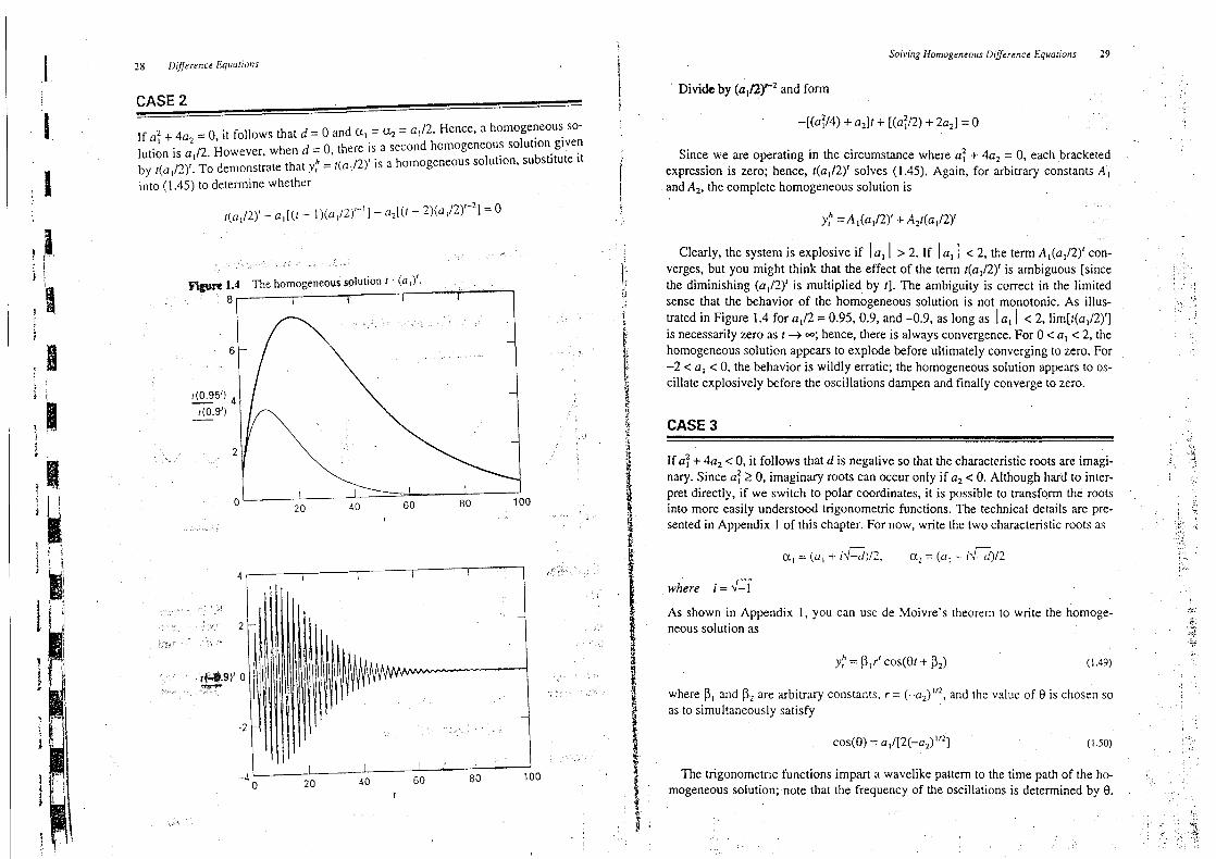
Sincc g., and c.c each solvc (1.45),

both tcrms in brackets mustequal zero. Assuch. the complctc homogeneous solution in thc sccond-order cas is

y =,4l(al)' + z4ctctzl'

l

Without knowing the specific values of 4), and tza. we cannot t'indthe two charac-teristic roots al and cez.Nevertheless, it is possible to characterize the nature of thesolution', there are threc possible cases tbat are dcpcndent on the value of thk; dis-criminantd.

!k'

CASE 1(

.) TJ-JLk. .( E (

' 2

If tj + 4z2 > 0. d is a real number and there will be two distinct real characteristgcrootstHence, there are two separate solutions to the homogeneous equation denotedby (a1)'and (c.,:1.We already know that any linear combination (lf the two is also asolution.Hence,

c., = ().5

. (a , +n-'d

)-

=0.? e,a= 0.5 . (a, - AJ-)=

-p.5

'l'he homogeneos solution is j' 0.7' + z

' (-0.5)'.The graph shows the.

time path of this solution for the casc in which the arbitrary constantyequalunity and t nans from 1 to 20.

CA';t 2: yj,) = 0.7y(, - )) + 0.35y(, - a). Hence, tzj = 0.7, al = t?.3.For'm the homogeneous equation'. y(,) - 0.7./,(,- 1)

- 0.35y(,- z? v 0.A check of the discririnant reveals J = (t2!)2+ 4 . az so that d = 1.89.

' g ' .. ..'.( '

., .Given that d > 0, the roots will be real and distinct..'ll'.'i : i

...' . Fonn the characteristic equation'. u' - 0.7 . a-l - 0.35 - a'-2 = 0

' ' Computethe two characteristic roots'.

c., = 0.5 .

a l + f-d),

= l.037 =(). 5 - (a ,

- T-d)=

-0.337

The homogeneous solution is A)- 1.037/ + Az . (-0.337),. The graphshowsthe time path of tlis solution for the case in which tbe 'arbitrary con-smntsequal unity and t nlns from 1 to 20.

Case 11

0.5.

5

0 10 20

Case 22.5

1.5

0 10 20

In he second 'exmple, y, = 0.7y,-, + 0.35y,-2.The worksheet indicats how to '.

E

. .obtainthe solution for the tp'o characteristic roots. Givn that one characteristicr .root is (1.037)1.the (y,) sequence explodcs. 'I'he intluence of the negative root. ,

; jj skrjtya' (a =

-0.337)

is responsibl for the nonmonotonicity of the t me pat .(-0.337)'quickly apprmches zero. the dominant root is tlie explosive value 1.037.

. )-' j

1

I

E tIj-M(

' yh = zt (aI)' + gztc.al'l

lt should be clear that if the absolute value of either c.! or c,zexceeds unity. thehomogeneoussolution will explode. Worksheet l

.1

examines two second-orderequationsshowng real and distinct characteristic roots. ln the first example. y, =

0.2y,-!+ 0.35y,-c, the characteristic rxt.s are shown to be aj = 0.7 and cta = -Q..Hence, the full homogeneous solution is yth= z4l (0.7)r+ z't:t (-0.5)r.Since both roots

are less than unity in absolute value, the homogeneous solution is convergent. As

you can see in the graph on the bottom left-hand sde of Worksheet 1.1, conver-

genceis not monotonic because of the influence of the expression (-0.57.

WORKSHEET 1.1 Homogeneous Solutions: Second-order Equllons

CASE -i

: ' '(,) = 0.2y(, - j ) + 0.35y(?- c). l-lcncc, rJ1 = ().2. az = 0.35. .

Fof'm the homogeneous equation'. )'j.) - 0.2y(,- 1)- 0.35y(,- )

= 0.

A check of the discriminnnt reveals d = (/1)2+ 4 .

az, so that d = 1.44.

Given that d > 0, the roots will bc real and distinct.

Let tbc trial solution have the form y(,) = a?. Substitute into the homoge-nous equation a' .=

0.2 . (f-' - 0.35 - a'-2 = 0

Divide by ct'-2 in ordcr to Obtnin the chnractelistic equation:ctl- 0.2a - 0.35 = 0 ;; ., , ,' .E. ) ,t .'

Compute the two characteristic roots:

!

f

I

Dtjlrence Equations

CASE 2.

; r LU '7f LQ-JJL---.--V q7 T 2

lf (zl + zlwz = 0, it follows that d = 0 and aj = h = akll. Hence, a homogeneous so-

lution is akrl. However.when d = 0. there is a second homogencous solution given

ph l

'

by latrl) . To demonstrate that y, = tajllq is a homogeneous solution. substitute it

into(1.45)

to determine whether

Solving Homoseneous Dllrrrlce Equa:ions 29

Divide by apjbn and fonn

-((422j/4)+ (7l + ((J21/2) + 2tzz) = 0

Since we are operating in the circumstance where tz2, + 4/: = 0, each bracketedexpressionis zcro; hence, taqlllt solves (1.45).Again, for arbitrary constants

,4l

and#z, the complete homogeneous solution is

nh=A!(J,/2)' + hztatllkf ' E.'

. . .'

. ,;

;. .

Clearly, the system is explo'sive if ltz, I> 2. If 1tz, l < 2. the term z4,(J,/2)' con-verges,but you might think that the effect of the tenn tablll' is ambiguous (sincethe diminishing abllj' is multiplied by J). The ambiguity is correct in the limitedsense that the behavior of the homogeneous solution is not nionotonic. As illus-

d in Figure 1.4 for akll = 0.95, 0.9, and-0.9,

as long as Itz: l < 2, limEl(ul/2)')tratei aril t

-+

co; hence there is always cnvergence. For 0 < a < 2 thes necess y zero as , ,

homogeneous solution appears to explode Yfore ultimately converging to zero. For-2 < tzl < 0, the behavior is wildly erratic; the homogeneous solution appears to os-cillateexplosively bcfore the oscillations dampen and nally converge to zero.

CASE 3

If (z2, + 4/: < 0, it follows that d is negative so that the characteristic roots are imagi-nary.Since (22, k 0, imaginary roots can occur only if az < 0. Altiough hafd to inter-pret directly, if we switch to polar coordinates, it is possible to transfrm th rootsinto more easily understood trigonometric functions. ne tecnical details are pre-sentedin Appendix l of this chapter. For now, write the two chafacteristic roots as

(y,I = ((zI + if-jlll, (y,z = (t7) - fV.C/24

:E j(.

. .L.,1.((7...

.'

:

..E.. ;

.,.j 1.E. :;8!*'''''''

lE'jj6.:1'Lq.'i'''.'.' ...

' '(.' .T:'.'7!

qtq3L.'.E:.

'. .

'.. jyWq'''' 14)4ijt (g)) . ..

?)tE kE

.#,

r

-2

-40 20 40 60 80 100

where i =-1

As shown in Appendix l , you can use de Moivre's theortm to Write the homoge-neoussolution as

yh = jlygcosto; + %)t

wherei'Jjand jz are arbitrary constants, r =(-a)lJ2. and the value of () is chosen so

as to simultaneously satisfy

l r2coslo) = (z1/(2(-tu) )

ne Zgonometric functions impart a wavelike pattern to the time path of the ho-

mogeneoussolution; note that the frequcncy of the osillations is determincd by 0.,

'

) '.

. j,

,

' ) .' ; '

34 Dtgrence Equotions

Sincc costgl) = costza + 0. thc stability condition is determined solely by the:J2. lf Iaz I= l . the oscillations are ofbunchanginj amplitude;magnitudcor r = (-t7z)

the homogcneous solution is pefiodic. The oscillations will dampen if az 1< l andexplodeif Iaz I> 1.

EXAMPLE: It is worthwhile to work through an exercise using an equaton withimginary roots. The left-hand side of Worksheet l

.2

examines the behavior of theequation y, = 1.6y,-j - 0.9y?-c.A quick check shows that tbe discriminant d is nega-tive so that (he characteristic roots are imaginary. lf we transfbrm to polar coordi-nates, the value of r is given by (0.9)1r2= 0.949. From ( l

.50).

coslo) = l.6/(2

x0.949) = 0.843. You can tlse a trig table or calculator to show that 0 = 0.567 (i.e.,ifcosto) = 0.843. 0 = 0.567). Thus. the homogeneous solution is

..) yth= ;j(O.949)' cos(0.567l + pzl

''f'hegraph on thc left-hand side of Workshcet 1.2

sets j)l= l and j:t = 0 and plotsthe homogeneous solution for t = 1. ..., 25. Case 2 uses the same value of az (hence,r = 0.949) but sets aL =

-.0.6.

Again, the valne ot-J is negative; however, for this set'

of calculations, costo) =-0.316

so that 8 is 1.25. Comparing the two graphsk youcnn sce tat increasing the value of 0 acts to increase the frequency of the oscilla-tions.

Given costo), use a tlig table to find 6

t; - 3.567 ij = l.25

WORKSHEET1.2 IMAGINARY ROOTS

CASE 1

y,- l

.6.3,,-,

+ 0.9y,-a

CASE 2

y, + 0.6y,-I + 0.9yt-c

(d) Form the homogeneous solution:y) = glP costof + j3z)y? = )1(0.949/cos(0.567? + ;$a) y) = j,(0.949)'cost l

.25/

+ )a)For jsy= 1 amdX = 0, the time paths of the homogeneous solution arr

2

g'

$'

E.

;'''.

.'.'

.'

:..

;'

tk7!1--...

1 25

Stabilitv Conditionsne general subility conditions can be surnmarized using triangle ABC in Figure1.5.Arc A0; is the boundary between Cascs 1 and 3) it iq the locus of points suchthatd = cl + 4c: = 0. ne region above z40# cohzsmnds to Case l (sinced > 0) andtheregion below A0# corresponds to Case3 (sinced < 0).In Case 1 (in which the roots are real and distinct), stability requircs that thelargestroot be less than unity and the smllest root be greatr than

-1.

ne largestcharacteristicroot, (r,: = (f)j+ VJ1/2,will be less than unity ifi

i t: + (u2+ g.u )1r2< 2,I 2!? Hence,t71 + zuc < 4 - zkzt + (24

lror

)'

.-

' i.

j '1

:

z j. ja g ..

u(ck+ a < !

(a) Check the discriminant # = tz2, + 4th

d = (0.6)2- 4(0.9)

=-3.24

H4peekthe roots are imaginary. Thc homogencous solution has the form

yh = jjr.fcostol + )al!

Where ;J1and fzare ttrbitrar'y constants.

(b) Obtttin the value of r = (-az)'r2

r = (0.9):C2

. .. ).2

E'.. ;. ..: i.

. t i (.k

= 0.949

A F''-'''j,

j! .j''

a- (t?2+ 4c )1'2>

-2

.

1 1 2

az < 1 + a ,

Thus. the region of stability in Case l consists of a1l points in (he region bounded

by KQBC.For any point in AORC,conditions (l.52)

and (1.53) hold and d > 0.

ln Case 2 (repeatedroots), tz12 + 4tz: = 0. The stability condition is Itz, l < 2.

Hcnce, the region of stability in Case 2 consists of a1l points on arc d4OS.In Case 3

(d < 0). the stability condition is r = (-f7c)lf2< ! - Hence,j .

..

.

(wherea: < 0)

Thus, the region of stability' in Casc 3 consists of a1l points in region z10P. F9r

anypoint in z10S,(l.54)

is satisfied and J < 0.

A succint way to charactelize the stzbility conditions is to state that the charac-

teristicroots must 1ie within the unit circle. Consider the semicircle drawn in Figure

I.6.

Rcal numbers are measured on the horizontal axis and imaginary numbers on

Sclvfng Homoseneous Di/yrencr E'tputlltm.s 33

Figure 1-6 Choctehstic roots and the unit circle.

t)!

thevertical axis. If the characteristic roots al and c.zare bot real, they can be plot-tedon the horizonul axis. Stability requires that they 1iewithin a eiwleof radius 1.

Complex roots Fill lie somewhere in the complex plane. If a: > 0, the roots al =

ltzj+ i-dyl and tra = (tzI - if-dlll can bc represented by the two Xintsshown iFi ure 1.6. For example, (y,l is drawn by moving atll units along the real axis and

J/2 units along the imaginary axis. Using the distance formula, we can give thelengtl of tle radius r by

r = (Jj/2)2+ dnilzjl

andusing the fact that il =

-i,

we obtain

r = (-tzz)IN.

.. (E

','I'he subility condition requires that r < l . Hence, wben plotted on the corplexplane,the two roots aj and c.cmust 1ie within a circle of radius equat to unity. In '

''

th i-selies

literature, it is simply stated that stbilty requires that all charac-e t me )i tic roots lie wthn the unit circle. .' ; )l r J

. .'(Higher-order Systems. .r

differenceequatiohs. ne homogeneousequatid foi (1.10)i;

Dljjrena Equations

a . = jl

i = I

Given the results in Section 4, you should suspect each homogeneAi solution tohave the form y) = Aa', where ,4 is an arbitrary constant. Tbus, to 111'1tbe valuets)of a, we seek the solution for

1 -

cl - c; - fla > 01+ t:I -

a; + ca > 01 - a l az + az - c2,> O3 + t:j + al - 3;3 > 0 orr, dividing through by '-n

wz seek the values ot- a that solve. 9

zl . a (y,a- 1

- a a.n-2. . . .( 2 :z: ()Q 1 2 n

3 - t'j + az + 3f)3> 0Given that the first threc inequalities are satissed, cither of the last two can bechected. One of the last conditions is redundant given tht the othor three hold.

7. FINDINGPARTIUULAR SOLUTIONSFORDETERMINISTIC PROCESSES

'Finding the particular solution to a difference equation is often a matter of ingcnu-ity and perseverance. ne appropriate technique depends crucially on the form ofthe (x,)process. We begin by considering thosc processes that contain only deter-ministiccommnents. Of course, in econometric analysiss tile forcing process willcontainboth deterrninistic and stochastic components.

CASE 1. --. -- ).. )-..L-

- -. .. . . . .. ).- . - . . . -- . -. . --..-- -- J'

..-

kt - 0. When a11elements of te (1,)process are zero, the difference equation e-Comes.

j?t = Jo + fzll'r-t + t7zFf-z+ ''' + anyt-nIntuition suggests that an unchanging value of y (i.t., y, = y,-) = ... = c) Shouldsolvethe equation. Substitute the Zal solution y, = c into (1.58)to obtain

1 t30 a

(1.57)

This nth-order mlynomialwill yield n solutions fbr a. Denote these n character-istic roots by aj. aa. ..., aa. iven the results.in Secton 4, the linear combinatibnAlal + Ac + ... + Ana'a is also a solution. The arbitrary constants Al through hncan be eliminated by imposing n initial conditions on the general solution. The .ai

(may be real or complex numbers. Stability requires that a11 real-valued (y,j be lessthan unity in absolute value. Complex roots will necessarily comc in pairs. Stability''requires that a11rot?ts lie within the unit circle shown in Figure 1.6.

iln most circumstances, there is little need to directly calculate the characteristicroots of higher-order systems. Many of the technical details are included inAppendix 2 to this chapter. However, there are some useful rules to check the sta-bility conditions in higher-order systems.

1. In an nth-order equation, a necessary condition for a11characteristic roots to 1ieinsidethe unit circlc is

2. Sincc thc valucs of tlle ai can bc positive or negative, a suftscient condition fora11charactcfistic roots to 1ieinside the unit circlc is

nju

ju j' i

.'.

. . . . .. i = 1 .) (

.:. ..'

. ( . ': . . .;r . . ... ; . .r.:. . t .. . .

.'.

..,qj.t

: ..., .? ...: . :.(..?..... .. .. .. ..: .q....

.E :.( ;

.

.'.'. .;. . ,.:.t.....

.;.)i;.?tEt@'t!!.;. : .j;;3.L.i ;...

... :, .. ..

: '

. ... E !

3

Aj ryt jv: , t,,!

g j g ji. : guajj; u j) ktj. ;fi '

. . . . . .:

... . ) .. . .. .

,.r ..

g.(.

#>i

1!iI

:..'

! c''i.4;.,*Til'l.p;d1C'

''

'

4

D1J-ere n ce Equa f t'o n .

As long as- a - (;z -. - (1,,) doq)s j1':)( ttqual zcro. lhe valuc of c givcn by

(1.5t.))

is a solution to (l.58).

Hence, thtt particular solution to (i.5s)

is given by

v,P = t7(/( 1 - tzj - az - ... - av,).

If l - t7: - az- ... - an = 0, the value of c in ( l

..59)

is undefined-. it is necessafy to

try some other form for the solution. The key insight is that (yp) is a unit root

processif L'zk= 1. Since fyf) is not convergent. it stands to reason that the constany

solutiondoes not work. Instead, recail equations ( l . 12) and (1.26),.

thesc solutions

suggestthat a linear timc trend can appear in thc qolution of a unit root process. As

snch. t;'y thc solution yr = cJ. For CJ to be a solutitln. it must be the case that

or combining like terms. wc obtain

For example. !et

y, = 2 + 0.75:,-1 + 0.25y,-:.

Here, t7I = 0.75 and az = 0.25) (y,) is a unit root process since tzy + az = l .

'f'he

particular solution has the form cJ, where c' = 2/:0.75 + 2(0.25)) = 1.6. ln the event

that the solution ct fails, sequentially (1-y the solutions y: = cr2, cP, -..

, cf. For an

nth-order tquation. one of these solutions will always be thc particular solution.

CASE 2.

The Exponential Case. Let A; have the exponential form bd)r where b, ti and r

are constants. Since r has the natural interprcttltion as a growth rate, we would ex-

pect to encounter this type of forcing process case in a growth context. We illus-

trate thc solution procedure using the tirst-orderaquation;

= t2 + a 4y,- I + ltr

A ()

To try to gain an intuitive fcel for tbe form of thc solution. notice that if b = 0.

( l.60)

is a special case of (1.58).

Hence, you shoul expect a constant to appear in

the pmicular solution. Moreover. the expression t/r' grows at the constant ratc r.

Thus, you might expect the particular solutit'n to have the fonn y; = ctj + cslrr,

where ctl and c! are constants. If thts equation is actually a solution. you sbould be

Finding rtzrficulcrSolutionsjr Delennfafllic Procenes

able to substitute it back into (1.60) and (lbtain an identity. Making the appropriatcsubstitutions,we get

c + c,r = a, + c,fco + c,'t-l'j + bro

For this solution to e'work.'' it is necessary to select co and cl such that

o = a4 ! - t:1)

Thus, a particular solution is

The nature of the solution is that.yr

equals the constant t7J(1- t7I) plus an ex-ipressionthat grows at the rate r. Note that for Idr 1< 1, the particular soluticn con-yergesto al 1 - tzl).2 ('

.,f'.b

If eithcr tzl::lz 1 olr tzl = dr%use the Sttrick'' suggested in Case 1. lf a ;

= 1, try the .'

I

solutiono = ct, and if tzl = Jr, trv the solution cj = tbdrydr- tzI). Use precisely the'

t.v'

.j... .y..,...j

samemethodology in higher-order systems.

ASE 3

Determlnistic time trend. In this case let the (x ) sequence be represented by the' l

relationshipxt = btd where b is a constant and d a msitiveinteger. Hence,

Since yt depends on td, it follows that y,-, depends on (J - 1F,yp-z depends onu .

.

(1 - 2),i etc. As such, the particular solution has the form yr = o + cII + c1f + ''' +

cZ.To find the values of the ci, substitute the particular solution into (1.62). Then . . E

1 t the value of each c that rcsult in an identity. Although various values of d areseec i

Nssible, in economic applications it is common to see models incorporating a lin-ear time trend d = 1). For illustrative puqoses. consider the second-order equation

y,= av + tzyyf-: + aob-z + bt. Posit the solution yr = o + ckt, where co and cl are un-determinedcoefficients. Substituting this Stchallnge solution'' into the second-orderdifference equation yields

( l.63)

Now select values of co and cj so as to force Equation (1.63) to be an 'identity fora1lXssiblevalues of J. If we combine a11constant terms and a1l terms involving 1.

therequired values of co and cj are

R

311 Dtgerence Eclzzllftpl.s

so tha:

Thus. the parlicular solution wil! alsw wkplltain

a linear time trend. You shouldhave no difficulty foresceing thc solution technique if tzl + az = 1. ln this circum-qtance which is applicable to higher-order cases als-t:'y multiplying the originalchallenge solution by 1.

8. THE METHOD OF UNDETERMINED COEFFICIENTS

At this point, it is appropriate to introduce the tirst of two useful methods of sndingparticularsolutions when there are stochastic components'in the (y,)process. nekey insight of te method of undetermined coemcients is tat the particular solu-.tion to a linear difference equation is neccssarily lincar. Moreover, thc solution candependonly on time. a constant. and the elements of the forcing prcess (xr).nus,it is often possible to know the exact/br?n of the solution even though the coeffi-cients of the solution are unknown. ne techniquc involves posiling a solutioncalled a challenge solution-tat is a linear fundtion of a11terms thought to appearin actual solution. ne problem becomes one of Iinding the set of values for theseundetenninedcoefficients that solve the difference equation.

ne actual technique for finding the coefscients is straightfonvard. Substitute thecballengesolution into the otiginal difference equation and solvc for the values ofthe undetennined coefficients that yield an identity for al1possible values of the in-cludedvariables. lf it is not possible to obtain an identity, te form of tlle challengesolution is incon-ect. T:-,,/ new trial solution and repeat the process. In fact, weuscd thc mctod of undetennined coefficients when positing te challenge solu-tionsy,# = co + cl drt and y,# = o + cj t for Cases 2 and 3 in Section 7.

To begins reconsider thc simple first-order equation yt = ao + tzly/-j + E?. Sinceyou have solved this equation using the iterative method. the equation is useful forillustratingthc method of undctennined coefficients. ne ature of the ly,)processis such that the particular solution can depend only on a constant term, time. andthe individual elements of the (6,) sequence. Since t does not explicitly appear inthe forcing process. , can be in the particular solution only if the characteristic rootis unity. Since the goal is to illustratc tc method, posit the challenge solution:

yt = h + bjt + ktt-i

j'= ()

wherc bok 1. and a11the xt are the coefficicnts to be dctermined.

Substitute (1.64)

into the original difference equation to form

Collecting like terms, we obtain

Equation (1.65)

mnst hold for a11valucs of t and all mssiblevalues of the (E,)sequence. Thus, each of the following conditions must hold;E

ao - 1 = 0c.l -

a l %.= 0cta- tzjtzj = 0

bo-

ao - tzl)o + tz1?, = 0bL - tzjl'j = 0

Notice that the fifst ser of condions can l)e solved for theqc./recursively. ne so-lutionof the first condition enmils setting W)= 1. Given this solution for cmvthenext equation rcquires a: = cl . Moving down the list, we obtain az = tzlat ortt,z = tzl. Continning te recursive process, we 5nd cg = f'j. Now consider th lasttwo equations. nere are two possible cases dernding on the value of aj. If 411 # 1.it immediately follows tbat bk = 0 and bv = a 1 - t71). For this case, te particularsolution is

Compare this result to (1.2

1)-.you will see that it is precisely the same solutionfound using the iterative method. Tbe general solution is the sum of this particularsolution plus the homogeneous solution z4cj. Hence, the generl solutitm is

Now. if there is Rn initial condition fof yo, it follows that

I)'

, !

It

Thr Afz-r/ltlt/of L/nt/crt.r?rl/lirr/Cotpjlcirnts

h +#!f + Jwa4,s.*,% '#J. I h + bt t - 1)+ (&E?-!-'. + s.+ ;$1E,-,

i;zz() .. k.tE;. ()

Mixch.ing oeflicients on all terms containing E,, E,-: . E,-2, ... yields

! ( ( ( :y ( W = )c.l = a 1+) + ;J, (so that aj = a j + flll)ac = t7l(y,l (sothat cec= t'J,((J: + ;'$j))az cut tzjaz . (sothat aa = (t7l)2(c;+ ;Jj))

a.i = a jaj-: tso that t.i= (z,)i-'(Jl + j1))

bv= ao + tzlbo - fzlbl

b j= a 1b!

To take A 'cotjd' example. consider the equation

y,= t'o + a .y?-I + E, + ;Jlt,.-!

Again, the solution can depend only on a constant, the elements of the (E,) se-quence.and t raised to the Grst mwer.As in the previous example, l does not need

to be included in the challengr solution if the characteristic root differs from nity.

To reinforce this point. use the challenge solution given by (1.64).Substitute tis 'tenmtivesolution into (1.67) to obtain $

. .:'.. . . .

The general solution augments the particular solution with the term.4t7l.

You areleftwith th'e exercise of imposing the initial condition for yll on thc general solution.Now consider the case in which cl = l . The undetermined coeficients are such that

''

:j = ao and bo is an arbitra:'y constant. The improper form of the solution is .'

42 trencefvualion.

.'

. . . ' . . . . . '.

.

'' ..': .: ...'. .1'!' '. E.

'. ..

z.' (.. ...

' ' 1:'?

Higher-order SystemsThe identical procedure is used for higher-ordcr systclni .iA.wtlexarttj 1tj ld ut hdthe particular solution to the scconfl-rnrtl'zr equation: E.. .'

',' = /7 + a jyr-j + aj ,-a + et.1 O

Sincc we have a sccond-order equation. wc use tllc challengc solution:

= bo + bLt + 172r2+ %e, + a1E?-l + (.cEt-2 + .'.F,

43

( l.69)

must equal zero for a1l values of J. First, consider the case inwhichfll + (72 # 1. Since (1 - t:21 - azj does not vanish. it is necessaly to sct thevalue of bz equal to zero. Given that bz = 0 and the coefticient of l must cqtlalzero, it follows that bt must also be set equal to zero. Finallg, gi.ven thatb, = bz = 0, w.e mtlst set bo = J#(1 - (71 - azj. instcad. ir Jt + tzz = 1. the solu-tions for tht bi depend on the specitk values of aw t7:. and tzz. 'I'he key point isthat he .&J2!)ifl'ly condition for the homogeneous equation is precisely the condi-tionfor convergence of the particular solution. J./-the characteristic roots of thetprrlo/anct?lt.tequation are elftzl to uafy, a polynomal time trend will appearin the particular solution. ne order 4./ the polynomal is the number of unitarycharacterisc roots. This result generalizes to higher-order equations.

Equation

If you are really clever, you can combine te discussion of the last section withthe method of undetermined coefficiene. Find the detemnistic portion of the par-tcular solution usihg the techniques discussed in the last section. Then use themethodof undetcrmined cllefficient-s to find the sthastic portion of the particularsolution.In (1.67).for example, set E, = E,-) = 0 and obtain the solution :(/(1 - /j).Now use the method of undetermind cfficients to find the prticular solution ofyt = (7lyf-, + Ef + pIe,-1. Add together the deterministic and stochastic componentstoobtain a11commnents of the particular solution.

A Solved ProblemTo illustrate the methodology using a second-order equation, aagment (1.28) wiihte stochastic tefm G so that

= 3 + 0.9y,-l - 0.2y,-z + 6,F?( l

.70)

Yot) hnve already vrfifittd tlmt the two homogeneous Solutions are Aj(0.5)' andz(0.4)'and tlle deterministic Portion of the particular solution is y,# =) 10. To findthestochastic portion of te particular solution, fonn the challenge solution-. '

*

y: = aiEt-

=0!

:

. y. .

;'

2. 4

'

1ln contrast to (1.64),

the intercept term bo is eicluded (sincc we have already.'''

)ftmndte deterministic portion of the particular solution) and the timc trend btt isli h teristic roots are less than unity). For this clk.v -rige

toexclnded(sincebot .c arac

. ., .

,

%%W0rk'* it must satisfy%

09( E + a E + ct E + d E +.1.

)''

l%6, + (:16,..1 + Xg't-.z + (2t3G.-:I + .*. =

. (1(j ,-1 j t-, c ,..:j zj tu. .. ;- 0 ztc/oe+ a E + %et-4+ daE,-,s + ... J + e (1.71)> t--:j l 1-- :1.

r

where#o, '1, bz. and the (J.; are thc undetennined coefficients.Substituting the challengc solution into (1.68) yields

The necessary and sufficient conditions for tlle values of the af's to render theequation above an identity for a11possible rcaliz:ltions of the (E,) sequcnce are

co = 1c,, = llao gsothal ct! = 21)

cf.a= clay + azp (sothat ty.a= (tzl)2+ c(Ezy= 7ja..z + Jzty,! (sothat aa = (N$)3 + 2t7cz)

.. '

..

,'

'

q Cqq.. .... :q(F.

j

Norice that for any value of j 2 2. the coefscients solve the second-order diffef- )

encefrquation

c.y= tzlcs: + azhn. Since we know ao and ay. we can solve for all 7,the a, iteratively. The properties of the coeffidients will be precisely' those dis- 8

Jcussetlwhen considering homogencous soluticns. nantely the following: 5t

1. Convergence necessitates laz 1< 1, t?) + az < l . and az - cj < 1. Notice that con- (vergenceimplies that past values of the (E?) Fequence ultimately have a succes- t

sivelysmaller inuence on the currentvaluc of y,.2. lf the coefscients converge, convergence will be direct if (tz2j+ 4tzc) > 0, will

follow a sine/cosine pattern if tt + 4(7a) < 0. and will t'explode'' and then con-verge if tty+ 4az) = 0. Appropriatcly setting the i. we are left with the remain-ing expression: '

Dtjference Equa:ions

Sincc ( l.7

l ) must hold for a1l possible realizIgions gf :r, E,-y, Et-zy ---. ah of th

followingconditions must hold: ' ,,

fwg Oprralors 45

9. LAGOPEBATORS

If it is not important to know the actual values of tlle coefficients appearing in thepafticularsolution, it is often more convenient to usc lag operators than the methodof undetermined coefticients. The Iag operator L is defined to bc a Inear operatorsuchthat for any value y,

.' .,

i.- ,isa ) ,-i

Thus, Li prcceding y, silllply means to lag yf b i periods. 1(is useful to rememberthe following properties of 1agoperators:

1. The 1agof a constant is a constant: ,c

= c.2. The distributive law holds for lag o'perators. We can set (/ + Lhy',= Eiyt+ Liyt =

X-/ +.%-j.

3. The associative law of rhultipliction holds for lag operators. We can set L''Lly:=i ) i i j i+jL luyt) = Lyt.; = yt-i-i. Similarly. we can set L 1y, = lv y, = yt-i-j. Note that

!a0 = yyt r

4. L raised to a negative power is actually a lead operator'. L-k = y,.,.. To explain,define.j=

-i

and fonn Lih =y,s zuyt.vi.

5. For Ia l < l , the infinite sum (1 . alu + azl? + a3I).+ ...)yt

= ytjLj- ap. Thjsproperty of lag operators may not seem intuitivc. but it follows directly fromproperties2 and 3 above.

Proofk Multiply each side by ( l - aL) to form (1 - tz1.,)(1 + alu + a21,2 +(131,3+ ...)s

= yt. Multiply the two expressions to obtain (1 - alu + #/.a - alLl +21,2- a3L3+

...)y,

= yt. Given that la l < 1. the expression anLnytconvefges tozeroas n approaches infinity. Thus, the two sides of the equtin are equal.

1. l > l the infinite sum t l + (af,)-1 + (aL)-2 + (uIa)-3 +...1y,

=.-aluytl

'6. For a ,

(1 - aL).

cfo= lctj = 0.9%

go that al = 0.9, and fbr al1 i k 2,

aj = O.9af-! - 0.21/-2

Now, it is possible to solvc (1.72)

iteratvcly so that ct'a= 0.971 - 0.2% = 0.61 .

a3 = 0.9(0.61) - 0.2(0.9) = 0.369. etc. A more elegant solution method is to viewJ

(1.72)

as a second-order difference equation in the c,;with initial conditlons cto= 1

and a: = 0.9. The solution to ( l.72)

is...'4.'. . .'' .. ' .... . . .

.....x

4 0 4)fU-i= f (0.5)

- ( .

To obtain (1.73),note that the solution to (1.72) is af = A3(0.5) + A4(0.4)i,where

z43and :4zs are arbitrary consmnts. Imppsink the conditions (o = 1 and al = 0.9

yields (1.73).

If wc use (1.73).it follows that c.o = 5(0.5)0 - 4(0.4)0 = 1; c.j =

5(0.5)1- 440.4)1 = 0.9-,c.a = 5(0.5)2 - 440.4)2= 0.61, etc.The general solution to (1.70) is the sum of the two homogeneous solutions and

the deterministic and stochastic portions of the particular solution:

whercthe zi are given by (1.73).

Given initial conditions for yo and yI, it follows that l and Az must satisfy

Although the algebra becomes messy, ( l.75)

and (1.76)

can be substituted into( 1.74) to eliminate the arbitra:y constants:

... l - i ' '' ''Hence, y,/(l - aL) =

-(tz1,) '

,aL) yt .

i cc () '

Prooj Multiply by (1 - aL) io form (1 - JL)(1 + a'L)-! + (4,t)-2+ (J1-3 +...)

' y, =-aly.

Perform the indicated multiplication to obtain: (l. - aL + (ti)-'-1

+-2 - ttzfel-'+ a1.l-s - (47I-2 ...)y,

=-aluyt.

Given tht Ia I> l . the ekpres-alsiona-nlu-ny converges to zero as n approachts infinity. Thus. the two sides ofl

the eqtlation Jtre Cqual. '

Lag oprators.provide a concise notation for writing differnce equations. Using1ag operators, we can write the rth-orderequation yt uz ao + t7jyr-: + '.. +'apyt-p + E,

7r-

1

/ .)f/../''-

r.c/)ct. I.() ?t ( 2; l'( )., ?.'

or more conppactly as

z't(L).y = tJ() + tl

Alyt = ao + #(L)Ez

whereztsl and s(z,)are polynomials of ordcrs ;) and (l- respectvelv. . 2

diffe-rencecquations. iIt is straightorward to use lag operators to solve linearAgain, considcr the first-order equation y; - a. + ',).,-, + E,, where Ia,( < 1. usethcdefinition of 1. to orrr'

'

'

t!2

y, = tzfl + a 1,),, + e., (1.78) i,

&lg Operators

..' ) J5 :. .

:..

.. .

'

.. .( . .. ( y j...;

..

Lag Operators in Higher-order Systems t,. . . ( t (' . . . ..We can also use lag operators to transform the nth-order equatiol'' ' *'d E

+ t ' +3 ($ 1.5-1.aztn + ... + a,y-. + E, into

( 1 - a3L - azlvl - ... - a Lnjyt = ao + et

Or!

From our previous analysis (also see Appendix 2 in this chapter). we know thatthe stability condition is such that the characteristic roots of the equation zn -

lae-l - .-. -

an = 0 a111icwithin the unit circle. Notice that the values of a solvingthecharacteristic equaton are the reciprocals of the values of L that solve the equ-tion 1 - a L ..- - a f-,a= 0 ln fact, 4heexpression 1 - a L ... - aJn is then called thel zl *

1inversecharcteristic equation. Thus. in the literature, t is often stated tht the sta-bilitycondition is for the eharacteristic roots of (l - t7IL ... - anL to 1ie outside ofiheunit circle.

In principle, one could use 1agoperators to actually obtain the coefscients of theparticularsolution. To illustrate using the sccond-order case, consider y, = aj + 6f)/(1 - tzl. - azL2). If we knew the factors of the quadratic equation were such that (1- a3L - 2clJl = ( l - b,L) I - bzL). we could write

',= ao + E,)/( 1 - bbl 1 - bzl-lj

lf both /713nd bz are less than anity in ttbsolute value. we can apply property 5 toobtain '

.: .

'

Solving for y,. we obtain

yt = t7o+ Er)/( 1 - a 1.)

From propcrty 1, we know that Lzzo= az', so that ajlL1 - atL4 = Jo + tzltao + tz2jtzo +

...= (a#(1 - c!). From property 5, we know that 6,/( 1 - akL) = e, + Jle,-y + tzzjer-a +

... . Combining these two parts of the solution. wc obtain the particular solution

given by (1.21).For practice, we crln use 1agoperators to solvc (1

.67):

yt = ao + ajyt-b + E? + ))E?-j,

wherela, l < l . Usc property 2 to orm(1 - t,,c)y, = av + (1+ p,,)E,'. solvingfor

y,yields

y,= Ef7l,+ (1 + J31L)E,l/( 1 - (131.7

Expanding thc last two tcrms of (1.80)

gives the same solution found using the

method of undetermined cofscients.Now suppose y, = av + co./-, + E, but that lt7I l > l . The application of propcrty 5

to (1.79)

is inappropiate since it implies that y, is infnite. lnstead, expand (l.79)

in roperty 6:us g p

43

Reapply thc rulc to (l(; 1 - b ,) antl to cacl) of l tlc clcmcnts in thc summation

bi 8r,-f to obtai n the particular solufion. If you want tl.'lknow thc actual cocfficienls

of thc proccss. it is prcfrablc lo usc the lllctjlt'd

ot' undetornlincd coefcicnts. Tllc

beautyof lrlg opcr:tors is tht tl)c)' cla bt-..tlkkt-sl l() dvntte stlch parlicular soltltions

succinctly.Thc general lmodel

z(-l.y,

= t'Jt) + /(l.)E,

has thc particulktr soltltioh:

y, = afj/,,l 1.) + Bl-letlvh (L)

10. FORWARD - VERSUS BACKWARD-LOOKING

SOLUTIONS

As suggested by ( l.82).

ther is a forward-lotking solution to any linear difference

cquation.The text will not make much use . lf the forward-looking solution since

future realizations of stochastic variabls arc not directly observable. However,

knowinghow to obtain forward-looking solutions is useful for solving rational ex-

pectationsmodels. Let us return to the simplz iterative technique to consider the

forward-lookingsolution to hc first-order eqtlation A',= ao + f7lyr-l + %.Solving for

'l-I. we obtain

Fr-, ='-a, + 6,)/r7

I + A'r/aI

Updating one period yiclds

)', =-(t7()

+ 6.,.: )//t1 +,?+ kla

)

-Jo(t7-, I + /-12 + t-l-j:' +...)

converges to al l - t7:). Hence. wc can writc thc forward-lookingparticular solution for y, as

Notc tllat ( !.86)

is sil'nilar l 11 1'01'11) to (.I.82).,

the di ffcrcncc is ihat the./itllrtz

v.al-

ues of thc disturbances affect the prcsent. Clearly. it- lt,I I > l . thc summation isconvergentso that ( l

.86)

is a lcgitimatc particular solution to the diffkrcnce equa-tion. Given an initial conditiony a stochastic differencc equation will have a for-ward- and backward-looking soluton. For example, usipg 1ag operators, we canwritethe particular solution to y, = 2() + t-2:y,-l + E, as (t?()+ E,)/( 1 - (1 1,). Now multi-p1ythe numerator and denominator by -a; 1.-1 to fbrm '

t9 f d-looking solution for 'any nth-orderMore generally. we can always o tain.a orwarequation.(For practice in using the altcrnative methods o'f solving diffrencc cqua-tions,try to obtain this fonvard-looking solution using the method of undeterminedcoefficients.)

' jProperties of the Alternative Solutions

ne backward- and fonvard-looking solutions are two mathematically valid solu-tionsto any n.th order difference equation. In fact, since the equation itself is linear,it is straightforward to show that any linear combination of the fonvard- and back-ward-lookingsolutions is also a solution. For economic analysis, however, the dis-tinctlonis important since the time jaths implied by these alternative solutiops arcuite different. First consider the backwgrd-looking solution. lf lf7I l < 1. th.e ex- .q

pressioncJ$converges toward zero as i -+

x. Also. notice that thc effct of E,-/ on.vt

is cf; if Irll 1< I . thc effects of the past 6., also diminish ovcr time. Suppose istcadl 1 l - in this instance. the backward-looking solution for )' ex lodcs.tht tzj > , l

< 1, the ex-The situation is reversed using the forward solution. Here, if 1t7,

- ets infinitely large as i approaches x. lnstead. if Icl l > l , the for-gressiontzl gward-lookingsolution leads to a finite sequence for (y,). The rerason is that J-l '

con--.increases.Note that the effect (f E,+F on y? is c-I; if I lt l > I , thcvergesto .zero as l

et-fectsof the future valucs of :+i have a diminishing intluence on the current valuc0 y. ' ' ,From a purely mathematical point of view, xcre is no

''most appropriate'' solu-

tion.However, economic theory may suggest that .sequence' be bounded in thesense that the limiting value for any value in the sequnce is sllite.Ral interest

y = - (t7( ) + 6 , . 1 jla I + (&', ..z- al ,

- E , + c)/ ((1 1)2. l

.

2 2'

=- ((-Jk) + 6.,+ I )/t7y

- (ct()+ q,+t)/(t? : ) + ytyzla I )

=- (t't(,+ Er..) 3la)

- (tl)+ e,+.?)/(ti1)5!+ (.--fp..2.- t'ltl - E.t4.t!.)/(.t7l )'h

r.; lfEyk#.,.e+..in) that la , l < l - tl)is forwari-lot

'king solution wil l di vergc as Jt be- .

'. .t4h.$*s.

.yi'lf.kgsjjllly! Etlarge

. However. it t(1 j I > 1- tht expression a , goes to zero while

E

J

i C!1 j E:(1 :1

.k

/r)l;(rer e ,1 (-t' f:-t///t7 tp?l.

rttes. real per capita income, and many othcr economic variables can hardly be ex-pcctcd to approach cither plus or mins infinity. Ilnposing boundary restrictions en-tails using the backward-looking solution if ItJj l < 1 and the forward-looking solu-tion if Ia l I> I . Similar rcmarks hold for higller-order equations.

Cagan's Money Demand Function

Cagan's model of hyperinllation provdes an excellent cxample of choosing the ap-propriateness of forward- vcrsus backward-ltloking solutions. Lct thc demand rormoney take thc form

Fonk'ard- Versus fftzckw'zrt-l-tltlll'rlt Solulions

&()- b()ll + p)/7= (c,- ,rl)/$ = h() = m - (y.-c/+/1.# $)/k$= - l/$ = w)= 1/(1 + 0)%)- (z,(l + ;$)/j= 0 = fy.l = F(l + fJ)2

=:> i = /141 + )''+1

1: tomp. zt form, the particular solution can be written as

The next step is to find the homogeneous solution. Fonn the homogeneous equa-tion,ptwb- (1+ l/9)p, = 0. For any aritra:'y constant A&it is easy to verify that theSolution is

( ;)t Ir

Hence. the g4*.1 :olution is

If you examine (l.92)

closely, you will note that.the impulse respobnse Nnctionis1+/. .

a i rogches inntyconvergent; the expression (;'J/(1 + ;$)) cpnvcrge: to zero pp .

n1(- Pt = a - ;hs !

-' p:$ fs> 0 .'

where r?1, = logarithm of- tbe nominal money stlpply in t

p, = thc logarithm of price level in :/J,'+) = thc logarithm of the price levcl cxlAcctcd in period / + 1

The key point of the model is that the denland for real money balances mt - p,)is negatively related to the expected rate of intlation (pte..l- p/). Because Cagap was

interestcdin the relationship between inflaton and money demand, all other vari-

ables were subsumed into the constant a. Sincc our task s to work with forwartl-lookingsolutions, 1et the money supply function simply be the process

v'here m = thc average value of tlle rnoney supply6, = a disturbancc tcn'n with a mean value of zero

As opposed to the cobweb model, 1et individuals have fomard-looking perfectforesight so the cxpected pricc for t + l equals the price that actually prevails:

Undcr pcrfcct foresight. agents in pcriod t are assumed to know the pricc level int + 1. In tbe contcxt of the example, agents arc able to solve difference equations

and can simply ttfigure out'' thc time path of prices. Thus, we can wlite thc moncymarkctcquilibrium condition as

???+ E, - p, = ct - itppy1 - #,1

For practice. we use the method of undetcnnined coefficients tc obtain the par-'

ing the exercise using iticular solution. (You shotlld chck your ablities by repeat

lt''p'y-

)

However, the homogeneous portion of the solution is divergent. For (l.92)

to yield

a noncxplosivc pricc seuencc, we m'ust be able to set the arbitrary constant ejual

to zero. To understand the economic implication of setting A = 0, supposc that the

initial condition is such that the price levcl in pcriod zero is ;)v. Ir we impose this

in ilial condi titln, ( 1.92)

bectlmes

lo afithms and appm= 1. Temporac changes in the money supply behave in aninterestingfashion. The impulse response function indicates that/hir, increases inthe moncy supply. represented by the various E,.j, ssrve to increase the price levelin the current period. erhe

idea is that future moncy supply increases imply higherprices in the future. Forward-looking agents rcduce their current moncy holdings.wit.ha consequent illcrease in the currcnt price lcvel. in response to this anticipatctlinflation.

SUMMARY AND CONCLUSIONS

Time-series econometrics is concemed with the estimation of differencc equations' containing stochastic components. Originally. time-seties models were used forforecasting.Uncovering the dynamic path of a series improves forecasts since thepredictablecomponents of the seris c3n be extrapolated into the future. The grow-ing interest in economic dynamics has given a new emphasis to time-series econo-metrics.Stochastic difference equations arise quite naturally from dynamic eco-nomicmodels. Appropriately estimated equations can be uscd for the interprctationof economic data and fr hypothesis testing.

This introductory chapter focuscd on methods of tssolving'' stochastic diftkrenceequations.Although iteration can be useful, it is impractical in manywcircumstances.The solution to a linear diffefencc eq'uation can be divided into two parts: a parlicu-lar solution and homogeneous solution. One complicating factor is that the homo-geneoussolution is not unique. The general solution is a linear combination of theparticularpolution and all homogeneous solutions. lmposing n initial conditions onthegeeral solution of an nth-order equation yields a unique solution.

The homogeneous portion of a difference equation is a measure of the tldisequi-

librium''in the initial periodts). The homogeneous equation is especially importantin that it yields the characteristic roots; an nth-order equation has n such character-istic roots. If al1 the characteristic roots lie within the unit circle, the sefies will beconvergent.As you will see in Chapter 2, there is a direct relationship between thestahilityconditions and the issue of whether an economic variable is stationary ornonstationary.

The method of undetermined cocmcients and use of 1ag operators arc powerfultools for obtaining the particular solution. The particular solution will be a linearfunctionof the current and past values of the forcing process. In addition. this solu-i i an intercept tenn antl a polynomial fuption of time. Unit rootst on may contaandcharacteristic roots outside of the uait circle'require the imposition of an initialcodition for the particular solution to be meapingful. Some conomic models a1-1owfor forward-looking solutins; in such circumstances, anticijated future events

. .' . . .

'.

haveconsequences for the present period. r t .The tools devloped in this chapter are aimd at paving the way flpr the study oftime-serieseconmetrics. It is a cood idea to work 1l thc exertiss prese ted be-1owCharactristic roots, the method of undetermibed coeftkients and lag opera- '*

. . !torswill be encountered throughout the remainder of th text.

Examine the three separate components of (1.92).

The deterministic expression

m- c, is the same type of long-nln

t'equilibrium'' condition encountered on several

other occasions'. a stable sequence tends to convcrge toward the deterministic por-tion of its particular solution. 'Fhe second cfmpollent of the particular solution con-

sists of the short-run responses induced by lhe v:trious t shocks. These movements

are necessarily of a short-tenn duration because the coeftscients of the impulse re-

sponse function must decay, The point is that the particular solution captures the

overall long-run and short-run equilibrium behavior of thc system. Finally, the ho-

mogeneoussolution can be viewed as a measure of disequiliblium in the initial pe-riod. Since ( l

-91)

is the overall equilibrium solution for period J, it should be clear

that the value of po in (1.93)

is the equilibrium value of the price for period zero.Aftcr all, (1

.93)

is nothing more than (1.9

1) with the time subscript lagged t pei-

ods.'rhus,

the expression (1 + 1/p)' must bc zerb if the deviation from equilib-

lium in the initial period is zero.Imposing the requtrement that the (p/)sequcnce be bounded necessitatcs that the

g OR0 F21SO1tl tiO11bci

:

i('

E

r'

1 )1 r

Notice that the price in each and cvery pcried is proportion' Soth: meknvalue'

of the money supply; this point is easy to veri since all variabls gre xpmssedin

Ilference f'qltations

QUESTIONS AND EXERCISES

Bill added the homogeneous and parlicular solutions to obtain yt = aolq 1 - t71) +

(ElLv()- rt#( 1 - a :)),

A. Show that the two solutions are identical ror1tJ: I < 1.

B. Show that for t7! = 1, Jill's solution is equivalent to yt = avt + yo. Howwouldyou use Bill's mcthod to arrivc at this same conclusion in the case

a l= 1?

2. The ccbweb model in Sectin 5 assumed stalic price expectations. Consder analternativefonnulation called adaptive expectations. Let the expected plice in l

(denotedby p)#) bfza wcightcd average of the price in t - 1 and the plice expec-tationof thc previous period. Formally.

J7,*= c./,- l + (1 - c)J?)t, ,

Clcarly, when ct = l , the static and adaptive expectations schemes are equiv-alcnt. An intercsting fegture of ths model is that it can be viewed as a differ-

ence equation expressing the expected pricc as a function of its own laggedvalue and thc forcing variable p,-l. '

A. Find the homogeneous solution for p).

B. Use lag operators to 5nd the particular solution. Check your answer by sub-

stitutingyour answer in the originl differcnce equation.

Suppose that the money supply process has the form m,= m Ypmt-k+ E,, wher'c

m is a ccnstant and 0 < p < 1.

A. Show tllat it is possible to express mt+,, in tcrms of the known value mt andthC SCCILICNCO(Ep.+.I . 6r+a. ... ,

E/+n).

B. Suppose that aiI values of 6.,.,. for ? > 0 have a mean value of zero. Explain q

how you could use your rcsult in y'art A to rccast the money supply /1 pe-riods into tlle future.

B. Show that each of the backward-looking solutions is not convergcnt.C. Show that Equation i can be writtcn entirely in first differenccs-. that is.AA',= ao + 0.5Ay,-1+ 6,. Find the particular solution for Ay,. llint.. Dcfine

y,*= Ay, so that y,* = t'Jo - 0.5yI + Er. Find the panicular solution for y,* intermsof the (Et ) sequence.)

D. Similarly transfonn the other equations into their f'irst-difference form. Findthe backward-looking particular solution, if it exists, for the transformcdk ' 'equzt Ons.

Given the initial condition yo, tind the solution for y, = tzo -

y?-j + 6.,-

A researcher estimated the following relationship for the inflation rate (,n,):.

A. Supposc that in periods 0 and 1. the inflation ratc was 10 and 1l %, respec-tively. Flnd the homogeneous. panicular. and gcneral solutions for the in-flation rate.

B. Discuss the shape of the impulsc rtlsponse function. Given that tlne UnitedStatcs is not hcaded for runaway inllation. why do you bclieve that the rc-searchef'sequation is poorly cstinlated? '

. .Consider the stochastic process y, = af$+ t7z..,-2 + E,.

Find the homogeneous solution and detcnninc the stability condition.

B. Find the particular solution using the method of undetermined coefficicnts.

A. Show that the backward-looking partiular solution for pt is divergent.

Dtye r:/1 ce rt/ltz;?'f?t.

13.Obtain tllc forward-looking particular solution for p, in termsor the (rn,)sequence,ln forming the general solution. why is it necessary to assume

that the money market is in long-run eqtlilibrium? '

C. Find the impact mulfiplier. How does an incrcase in 111:+: affec: pt Provide

an intuitive explanation of the shapc or the entire impulse response func-

tiOn .

9. For each ot- thc following. verify that the positcd solution satisfics thc differ-

c ncc cquation . Thc symbols c. c(), an C!c,, denctc constants !

Appndix l 57

.F = C + 7 lr ()

J? = t- -F c-()(- l)'

. (

y = c + co(- l)' + 6 + E + e ...4 + ...

.l z z-2 :

10. Part l 2 Fcr cach of the fbllowing. determine whether (y,) represents a stbleprocess. Detenmine whether the charatteristic roots are real or imaginary and

the real parts alr positive or negative.

. . r' ' !k. ' e.

yt = 0.8,y,-T + e:- 0.5Ef-T

A Supposc that thc initial conditions arc such that l'u =

*0

and E() = E.-j = 0.Now sugposc that 6.l = l . Dctlttnlinc tllc valucs .yl through .v5 t)yforward i(-eration .

ENDNOTES

1. Another possibility is to obtain the folavard-looking solution', Such solutions are discussedin Section 1O.

2. Altemativtly, you can substitute (1.26)

into ( l . 17), Note that wbcn q, is a purc randomdisturbance, yt = c() + .v,-1 + E, is callcd a random walk plus dri model.

3. Any linear cquation in the variables .:1 through .:,, is homogeneous if haS thc Mrmljerl +azxz + ''' + d-?,,',, = 0. To obtain the bomogcncc... ortion of ( l . lO). simply slzt tlku lntcr-cept term a) and forcing process

.rt equal to zero. Hencc, the homogeneous equation for( ! , !0) is v, = a 1.),,- I + azyt-; + ... + a,vyt-n.

4. It' b > l'I. the demand and supply curves do no( intcrsect in the positivc quadrant. Thc as-stlmption a > b guarantees that the equilibrium price is positive.For example, if the, forcing process is x, = E, + fJ1E,.1 + pcE,-c + ...

, the impact multigliercan be taken as thc partial devative of y, with respect to xt. Howcver. this text fbllowsthe usual practicc of considering multipliers with respect to the (E, ) process.

APPENDIX1 Imaginary Roots and de Moivre's TheoremConsider a second-orderdifference equation y? = ajyp-y + tn?.)uz such that tbc dis-criminantJ is ncgative (i.e.,d = c2j + 4(2z< 0). From Section 6, we khow that thefull homogeneous solution can be wlitte' n in the fonm

hc zyt ctJ + A x1 l 2

wherethe two imaginazy characteristic roots are

c,l= (c, + fa/J)/2 a'z = (/1.-:

!

illll (A 1. 2)

The purpose of this appendix.is to explain hsk to rewrite and interet ( 1.1) interms of standard trigonometric funetions. You might

'rfirst

want to refresh' yourmemo'ry concerning two useful trig idcntities. For any two angles 81 and 0c.

sintoj + 0a) = sintol ) costoc) + costgl) sintoc)costot + 0z) = costot) cosloz) - sintol) sintoc)

lf 01 = ()z,we can drop subscl-ipts and form

sin(20)= 2 sinto) costo)cos(20)= costo) cost6) - sinto) sintg)

expressimaginaq numbers in the com'-plexplane. Consider Figure A 1. 1 in which the horizontal axis measures real num-bers and the vertical axis imaginary numbers. The ccmplex huniber a + bt can berepresentedby the poit t7 units. from the origin along the, horizontal axis nd b

The Grst task is to demonstrate how to

Dlgerence fltprt?ll.

- r,.,tt'-

a = ?. coste) b = r sin(0)

c,l = a + bi = rlcosto) + i sintMllxz= a - bi = rgcosto) - 1si n(8))

rj '

t)r

c.) = (rgcosto) + i si ! (0)1)(rgcostg) + i sintl) )= lcosto)costp) - sint6) sinto) + ll' sinto) cgstoll

#rom(A1.4).

:: .:.. . q.'.'.' ) '

a.:)= lcostzt)) .h t' sin(20)J

(EZJ= rzlcostrgl + i sin(;9)J

7 7

z'lj.= B, (costAc) + i sintfcllz

= 1?l(cos(#2)- f sin(:2)Jwhre #! and Bz are arbitrary real numbers measured in radians.

I: order to calculate A j ((z1),us: (A 1.6) and (A 1.7)

to folld

Using (A1 .3)

and (A 1.4),

we obtain

(A l.3)

'

Since S1 is arbitrac, the homogeneous solution can be writtcn in terms of the ar-bitrazyconstants Bk and Bz

z = B r' cost + Bzj (A1.1 1)f 3

Now imagine a circle with a fadius of unity superimmsed on Figurc A1.1.

Thestabilitycondition is for the distance r = Qbto be less than unity. Hence, in the liter-atureit is said that the stability condition is for the charactelistic roots to lie withinfhisunit circle.

APPENDIX2 Characteristic Roots in Higher-orderEqualionsz

ne characteristic equation to an ath-order differeace equation is

n n- ! ' a-2 k..(, = (;X - & Q - t7 U ' ' ', 2 rl

s stated in Scction6, the n val'uep of f that solve tis characteristic equationarecalled the characteristic roots. Denote the < solutions.'by cI, %, ..., c,,. Given

ppenda2 59

Since ythis a rcal number and al and tzc are complex, it follcws that A1 and amust be complex. Although Jth and A2 are arbitrac complex numbers, they rnusthavc the fonm

60 Dtjyrrnce Equations

the rcsults in Scction 4, the linear combination /t lc( + Azt7el+ ... + Angl ls also a so-Iution to (A l . 12).

A priori. the charactefistic roots can takc on any values. There is no restriction

that they be real versus complex nor any reszction concerning their sign or magni-tude.Consider the following possibilities:

1. All the %.are real and distinct. 'Fhere are several important subcases. First sup-pose that each valuc of ai is less than unity in absolute value. In this case, thehomogeneoussolution (A1.12) converges sincc thc limit ef each f.Lequals zero

as t approaches innnity. For a negative value of %, the expression (,; is positivefcr evcn valucs of t and negative for (dd values of . Thus. if any of the f,i arencgatve (but Iess than l in absolute value). the solution will tend to cxhibit

some oscillation. If any of the i are greater than unity in absolute value, the so-lutionwill diverge.

2. All the % are real but m f n of the roots :pre repeated. I-et the solution besuch that (y.l = c,c = ... = am. Call the single distinct value of this root a* and 1etthe other n-rrl root.s be denoted by tyvrr..lthrough cz. ln the case of a second-or-der equation wft.h a rerated. root, you saw tllat one solution was

z4lc,' and theother was Aztd. With m repeated roots, it is. easily veritied that Ja*: tlL*' ...

'

9 9 @

r-la*' are also solutions to the homogeneous equation. Wth m repeated roots,

te linenr combination o a11these solutions is

tenuinantsbelow are positiye, thc rval.parts or 1:411 haracteristic roots arc less tllan lin absolute value: '

1l

=

h '-J n

-J -J'J r: -- l

0 -a

N

I .-.a'

l

0 1

1 0 0 -.t'ln

-a I 1 O 0 -(:,,

-ac l O 0-n () I -(l

I

0 0 1-an 0 0

01

-a l

-J 4

-J 3

To understand the way each detenninant is formed, note that each can be parti-tionedinto four subareas. Each subarea of Af.is a triangular i x i matrix. The north-westsubarea has the value 1 on the diagonal and a11zeros above the diagonal. Thesubscriptincreases by I as we move down any column beginning from the diago-nal.

'fhe

southest subarea is the transpose of ths nonhwest subarea. Notice that thenortheajtsubarea has a. n the diagonal and a1l zeros below the diagonal. The sub-kript decreases by 1 as wc move up any column beginningfrom the diagonal. Thesouthwestsubarea is the transpose of the northeast subarea. As defined above. thevalueof Jo s unity.

Special Cases: As stated above. ti-leSchur theorem gives the necessar./ and suffi-i ditions for all roots to 1ie in the unit circlc. Rather than calculate al1 thesec ent con

determinants.it is often possible to use the simple rules discussed in Section 6.Those of you familiar with matrix algebra may wish to consult Samuelson (194l)forfonnarproofs of these conditions. '

'

3. Some of the roots are complex. Complex roots (which neccssarily come inconjugatepairs) have the fonn zi d: f0, where zi and 0 are real numbers and i isdefinedto be VX.For any such pair, a solution to the homogeneous equation isA tc.!+ f0)' + Aclc,l - f9)', where Al and z az.e arbitrary conrtants. Transform-ing to polr coordinates, we can write te associated two solutions in the formilr' costo? + jz) with azbitrary constants ;$1and ;$c.Here stability hinges on the

magnitudeof r'; if Ir I < 1, the system convergcs. However, even if there is

convergence.convergence is not direct since the sine and cosinc functions im-part oscillatory behavior to the time path of y,. For example. if tere are three

roots,two of which are complcx, the homogellcous solution has the form

jlr' costof + ;Jz).F.A3(x.q

Stability o Higher-order Systems) In practice, it is difficult to find thc nctual

values of the characteristic roots. Unless the characteristic equation is easily fac-tored, it is necessary to uSe numerical lethods to obtain the characteristic roots.However. for most purposcs, it is sufficient to know the qualitative properties of the

rolution;usuallys it is sufficient to know whether a1lthe roots 1iewithin the unit cir-

cle. The Schur theorem gives te necessary anl sufficient conditions for stability.Given the charactelistic equation of (A 1.12), the theorem states that if a11the n de-

1('

t

t < .J ..

<we

-.,

.)7()('). ..'.S;'

; r '

1.t

Chapter 2

SJATIONARY TIME-SERIES MODELS ty..

Thetheory of linear difference equations can be extended to allow the forcingprocess(x,J to be stochastic. This class of linear stochastic difference equations un-derliesmtlch of the theory of time-selies econometrics. Espccally imortant is theBox-lenlins (1976) methodology for estimating time-series models of th form:

yt = fltl + (1zyt- j + * * * + apyt-p + t + ;'lj f.J- j + ..* + jE/.t?

Such models are called autoregressive integrated moving average (ARIMA)i dels The aims of thist me-ser es m0 . chapter are to-.

Present the theory of stochastic linear difference equations and censidtr thetime-scriesproperties of stationary ARIMA models; a stationac XRIMA modelis called an ARMA model. It is shown that the stability conditions of the previ-

s chapter ar necessal'y conditions for stationarity.ou

2. Dcvelop.thc

tools used in estimating ARMA models. Especially useful arc teautocorrelation and partial autocprrelation functlons. It is shown how the'Box-lenkins methodology relics on these tools to estimate an ARMA modet

fromsample data.3. Consider various test statistics to check for model adequacy. Several examples

of estimafed ARMA models arc analyzed in detail. lt is shoW how a properlystimatedmcdel cnn be used for forecasting.1

/CSTOCHASTICDIFFERENCE EQUATION MODELSj,

'

..

i

this chaptcr. we continuc to work with discrete. rather than continuous, timb-serisJmodels.Recall fromE the discussion in Chapter 1 thaiwe' can evaluate

'the

ftmtion y = ftj at fo and to + to form j.

'.

1 ' 1.'' '' 'E1 -

tk :

.

!'

r ..r

.'

..

...'.

.' (.

764 Sationury Time'series VfJf/6/J

ty = .J(lo+ /)) - f #))

As a practica! mattcr. most economic time-serics data are collected for discrctetime periods. Thusv we consider only thc eqtlidistant intervals lo, Io + /), to + 2/1.J() + 3/7. . . . and conveniently set h = 1. Be cartrll to recognize. howevcr, that a dis-cretc time series implies t. but not necessarily r,. is discrcte. For example. althoughScotland's annual rainfall is a continuous vrlriable. the sequence of such annual

rainrall totals for years 1 through J is a discrcle tinle series. In many economic aI)-plications. : refers to

ttime-'qo thtt /? rcprcscnts the change in time. However. ;

need not refer to the type of time interval as nleasured by a clock or calendar.lnstead of allowing our measurement units to be minutes. days, quarters, or years.

we can use t to rcfer to an ordered event nulllbcr. We could 1ety; dnote the out-

comc or spin t on a roulette wheel; yt can then takc f)n any of the 38 values O0, 0, I ,

36.A discrete variable y is said to be a random variable (i.e.. stochastic) if for anl'

real number r, there exists a probability py K r) that y takes on a value less than or

equal to r. This degnitit?n is fairly general; in common usage, it is typically implied

that there is at least one value of r for which 0 < py = r) < l . lf there is some forwhichpy = r) = 1,y is deterministic rather (han random.

It is useful to consider the clements of an observed time series (y().y,. yz, . . . , F,Jas being realizations (i.e., outcomcs) of a stochastic process. As in Chapter 1. we

continueto 1et the notation y, refer to an element of the entire sequence (y,). In ourroulette example. y, denotes the outcome of spin : on a roulette wheel. lf we ob-

serve spins 1 through F. we can fof'm the sequence y:, yz, . . . . yr. or more com-pactly, (y,l. ln the sal'nc way, the term yr could be used to denott GNP in tire pe-riod t. Since we cannot forecast GNP perfectly, y, is a random variable. Once we

learn the value of GNP in period t, yt becomes one of the realized values from :4 sto-chastic process. (Of course, measuremclt error may prevent us from ever knowingthe

'ttrue''

value of GNP.)For discrcre variablcs, the probability distribution of y, is given by t formula (or

table)that siccifics each possible realized value of y, and the probability associated

wilh lhat l calization. If the rcalizations ara linked across time, therc exists the joint '

probability distribution p(),, = rl , yz = r2, . . . . yr = rr). where ri is the realized valpe.

of y in period i. Having obsewed the t'irstt I'calizations, we can form the expectd

value of y,+l. y,+2, . . . . conditioned on the observed values of y! through y;.1''liis

iditional mcan, or cxpected value, of %'twiis denoted by EtLyt.i1y;, y,-) . - . . ,

yI)'or lcon

F ,A', .i. i .

E

Of'course. if vt refers to the outcome of spinning a fair roulette wheel. the proa-'

bility distribution is easily characteriztd. l contrast. wc may nevcr be able to com- E

pletely describe the probability distribution for GNP. Nevertheless, the task of

economc theorists is to develop models that capture the essence of the truc data-

generating proccss. Stochastic diffcrcncc equations are onc convenient way of

modelingdynamic economic proccss. To take a simple example. suppose that the

Federal Rcserve's money supply target grows 3% each year. Hencc,

Stochasdc Dt#reace Equation Mode 65

n;* = 103?n*f*

r-- l

orgiven the' initial condition ?n'. the particular solution is

n = (l.03)//nt

where ?n) = the logmithm of the money supply target in year t/,21 = the initial condition for the ta-rget Illkplic/ supply in jeriod zero

Of course, the actual money supply mt and target need not be cqual. Suppose thatat the end of period t - 1, there exist ?n,-1 outstanding dollars that are carried

.for-

wardinto period t. Hence. at the beginning of t there arc ?n,-j dollars so that the gapbetweenactual and desired money holdings is mt - rl,-:. Suppose that the Fed can-notpedkctly control the money supply but attempts to change the money supply byp percent (p < 100%) of any gap betwen the desired and actual money supply. Wecanmodel this behavior as

Lmt = ptrn)k- rrl,-,) + E?

orusing (2.l). we obtain

mt = g( 1.Q3jtml + (1 - plmt-t + E:.

f24)

where e, = the uncontrollable portion of the money supply

We assume the mean of E; is zero in all time periods.Although the economic theory is overly simplc, the model does illustrat the key

points discussed above. Note the following:

Although the money supply is a continuous variable, (2.2)is a discrete differ-ence equation. Since the forcing process (E,Jis stochastic, the mtmey supply isstochastic;we can call (2.2)a linear stochastic difference equation.

If we knew the distribution of (E,), we could calculate the distribution for tach

elementin the (/7$)sequence. Since (2.2)shows how th realizations of the (rrI,)

sequenceare linked across tim, we would be' able to calculate the vrious jointprobabilities.Notice that the distribution of the money supply sequence is com-pletelydetennined by the paramters of the difference equation (2.2)and distri-butionof tbe (E,) sequence.

)'

'

Having observed the first t observations in the (rrl,) sequeqce. we cah hkeforecsts of znz.sj, zn,.c. . . . . For example, if we update (2.2) by one period and

. q t -. j . : q;..j.takethtconditional expectation, the forecast omt.., is p(1.O3) /71).#j.(

l plznr?+' l - )??,,.

.@

.:, .

iHece, E;%wt = p( 1.03) mt + ( p r . t

Before we proceed too fr along these lines. 1t 4s go back to the bastc building:

,

j.j j y.Llck of discrete stochastic time-series models: the W ite-no se process. A se-uencc (E,) is a whitc-noise proccss if each value in the 'sequence hs a mean of

Slat f-vltvz','.v Tibne- Serie5 /$/f l(1els

zcro, a constant variance. and is scrially uncofrelatcd. Fotm,ally, if the nqtg.tion F(.v)dcnotesthc thcoretical mean valuc of .v, tlw sequcnce (:4.) is a white-noiy processif fbr each timc pcriod r.

2. ARMA MODELS

It is possible to combine a moving average process with a Iinear differencc equa-i b i toregressive moving average model. Consider the pth-order diflt on to o ta n an auferenceequation:

('

E E?) = E(E,- I ) = . . . = O 7

a s z 2 2 ql

e,) = (6,-1) = ... = ()' !oy;lr(E,) = yar(6;.- , ) = ... = c

. t ,

j

r'

For each pcriod .-r, is constructed by taking thc values 6z, E,-!, . . . , et-q and mul-

tiplyingeach by the associated value of ;Jf.A sequence fonned in this manner iscalled a moving average of order q and denoted by MA(). To illustrate a typicalmovingaverage process, suppose you win $ l if a fair coin shows a head and lose

$1 if it shows a tail. Denote the otltcome on toss t by E; (i.e.. for toss t' e, is either

+$l or-$1).

If you wish to keep track of your''hot streakss'' you might want to cal-

culateyour average winnings oJ1 the last four tosses. For each coin toss t, your aver-

age winnngs on the last four tosses are 1/46., + 1/4E?-l + 1/4e.?-2+ 1/4E,-3. ln termsof (2.3),this sequence is a moving average process such that jj = 0.25 for i f 3 and

zero othenvise.Although the (6J) sequcnce is a white-noise process, the constnlcted (A'JJse-

quencewill not be a whitc-noise process if two or more of the fl differ from zero.To illustrate using an MA( 1) process, set jJ(,= ! . jl! = 0.5, and all other jsf= 0. lnthis circumstancc. Ext) = E; + 0.56,-1) = 0 tnd var(-v,) = vartEr + 0.56,-,) = l

.25c2.

You can easily convincc yourself that S(.r,) = E.':-sj and vart-r) = v r(.v?-,) for a1IJ.

Hcncc, the first two conditions fbr (.r,) to be a white-noise process are satisfie.However, f't-rrrl-ll = S((E, + 0.5e,- 1)(6,-

, + 0.56,-a)! = f(E,E,-I + 0.5(E,-I)2 + 0.5E,Ea7

+ 0.25E,-IE?-c) = 0.5c2. Givcn there exists a nonzcro value of s such that fR.rrv,-,)#0. the (-vr)sequcnce is not a white-noise process.

Exercise l at the end of tbis chapter' asks you to nd the mean. variance, and c()-varianceof- your

t'hot streaks'' in coin tossing. For practice. you should complete

that exercise before continuing.

We follow the convention of normalizing units so that Itl is always equal tounity.lf the characteristic roots of (2.5)are a!l in the unit circle, (y,) is called anautoregressivemoving average (ARMA) model for y,. The autoregressive part oftllemodel is the tdifference equation'' given by te homqgeneous portion of (2.4)and the moving average part is the 1.z',)sequence. lf the homoeneoud pal4 of thedifferenceequation contailis p lags and the model for xt q lags, the model is calledi

:an ARMAT,qj model. If q = 0, the process is called a pure autoregressive process1 .E denoted by AR(p). and if p = 0. the proccss is a gure moving average process de-E

jnoted by MA(). In an ARMA model, it is pedctly permissible to llow p and/or q' to be infinite. In thij chapter, we cotuider only models in which all the chiracteis-

q'

'tic roots of (2.4)are within te unit circle. However, if one or niore characteristicrooLs is greater than or equal to unity, the (y,)sequence is said ttj be an integratcd

!process and (2.5) is cailed an autoregressive integrated moving average (ARIMA)i odel. ' 'm

Treating (2.5)as a difference equation suggests that we canetsolve'' for y? in

E terms of the (e,) sequence. The solution of an ARMAI,qj model exprsing y., in( tenns of the (er)sequence is the moving average represention of yt. The procez!dure is no different from that dis'cussed in Chapter l . For the AR(1) model /, = 7() +

cyys.j + E;, the moving average representation was shown to be '

.t'

y, = aol l - (?j )+ 47lE,-j

i zz ()

For the general ARMAW,q4 model. rewrite (2.5)using lgg opefators so lhat

Fortunately. it will not be neccssary fbr us to expand (2.6) to obtain the speciccoefficient for cach element in (E,J. The important point to recognize is that the cx-pansion will yield an NIA(x) process. The issue is whether such an expansion isconvergent so that the stochastic difference equation given by (2.6) is stable. AS

you will sec in the next section. thc stability condition is that the characteristic rootsof the polynomial (1 - nil.v''lmust 1ieoutside of-the unit circle. It is also shown

.that

ir)', is a kllcttrstochasic t/tt-trrcncc eqtlaton, J/lc stabiliy t-t??lJflfr??li.%a nccc-unycondition for J/2t> time series /y,7:o be stationary.

and5.71 . Folnnally: a stochastic process having tt fihite men d varince is co-variancestationary if for all t and t-us, '

(2,7)

(2.8)

where /.t, trtrrtnd aI1y, are constants

In (2.9),allowing s = O means that yo is cquivalent to the variance of y,. Simplygtlqa time series is covariance stationary if its mean and all autocovriances aretmaffectedby change of time origin. ln the litcraturc, a covariance stationaryprocessis also referred to Jts a weakly stationary, second-order stationary, or wide-sensestationary process. A strongly stationarz process need not have a f'inite man

. and/or variance (i.c.. g and/or yo necd not be finitel', this terminology implkes thatweakstationarity can bc a more stringent condition than strong stationarity. Thetextconsiders only covariance stationary series so that there is no ambigtlity in us-i h terms stationary and covariance stationary interchangeably. One furtherng t eword about terminology. ln multivariate nodels, the term autodovarince is re-servcd for the covariance between y? and its own lagsk Cross-covariance refers tothe covaliance between one series and another. In univariate time-series mcdels,thereis no ambiguity and the terms autocovariance and covariance are used inter-changeably.E For a covarnce stationary series. we can define (he autocorrelation betwcen y,andyt-s as

px>'l-'o

3. STATIONARITY

Suppose that the quality control division of a manufacturing t-11-11,1samples four ma-chines each hour. Evtaryhour, quality control finds the mean of the machines' out-put levels. The plot of each machine's hourly output is shown in Figure 2.1. lf yitrcpresents machine yf's output at hour 1, the means @,)are readily calculated as

For hours 5, 10. and 15, these mean values are 5.57, 5.59, and 5.73, respectively.The samplc variance for each hour can similarly be constructed.. Unfortunately,

applied economgtricians do not usually have the luxury ot- bcing able to obtain anensemble (i.e.,multiple time-series data of the sante process over the same time pe-riod). Typically. we observe only one set of realizarions for'any particular series.Fortunately. if (y,)is a stationary series, thc mcan, variance. and autocorrelationscan usually be well npproximatcd by sufficiently long time averages based on tLesingle sct of realizations. Suppose you obscrved only the output of machine 1 for20 periods. If you kncw that the output was stationary. you could approximate themean level of output by

20.

= A'1,/20l

l = l

ln using this approximation, you would btt assuming that the mean was the samefor each period. ln tbis example. the means of the fotlr scries are 5.45, 5.66. 5.45,

Slalionary Tl'znt,-wh-trt'xkblodels

whercyoand yaare detined by (2.9).Since j and ya arc time-independnt. the autocorrelation coefficients p, are also

rime-independent.Although the autocorrelation bctwcen y, and .h-t

can differ from

thc autocorrelation between yr and yv-z, the autocorrelation between yt and y,-: must

be idcnticl to that betwccn yt-x and y,-.v-l. Obviously, p()= 1 .

Stalionarity Restrictions for an AR(1) Process :

For expositional conveniencc, first considcr the necessaryandEtpffiktt# onditions

(?. E.

.. .

' ' '

. ..,... j. .g . ?

for an AR( 1) process tl bc stationary. Let

y = (7fl + :11.).,- j + 6,(

E, = whitc noise

Suppose that the process startcd in pcriod zero. so that y() is a dctermnistic illitial

condition.In Section 3 of the last chapters it was shown that the solution to this

et uation is (also see Question2 at the end of this chapter)'

.)'

Updating by J pvriodsyields

I'

wc compare (2.1t) and (2.12), it is clcktr (llat bbth mcans are time-depenent.

incezfy;is no( equal to Eytws.the sequence cannot be stalionary. However, if t s

largc,we cnn consider tl)e limiting value of y, in (2.10).lf )tzl 1< l , the expression

tf7llrybconvergcs to zero as r becomes infinitely large and the sum J(,2 l + t7I.i.

i + (a))3+...)

converges to aqi 1 - J1). Thus. as l.-+

x and if l(7: l < l;a , )

Now 3:*4 4:>. . l/tpns of (2.13) so that for sufficiently large values of f, Eyl =

u t'i ite and time-independent so that Ey =

tdptl..z f!t). T . $. $h# mean value of yt is n ,

Stalionarl?y

'.y' = g for a1lJ. Turning to the limiting value of thc variance. we find(*-&

b, - 11)2= NIE, + a 6. j + (cI)76c +

...)2)

I 1..- 1-

= g2:. I + a I )2+ (t:7:)4+ ...j

= c2/( 1 - (aj)2j

whichis also finite and time-independent. Finally, it is easily demonstrated that thelimitingvalues of all autocovariances are finite and timc-independent:

-SIU?- h1)(,Vr-x- h1)1= Sl (E? + JIEI-I + (t7I)ZE,.-2 +-''1(6r-.

+ ('lj6,-x-I + (tzl)2Et-a-a +...)

).

2 . .

, I c 4

=C7(al)i. + fal) + (al) +-'-)

.= cztt7j)47gj - (tzj)2j

In summary, if we can use thc limiting value of (2.10),the (y,)sequenceswill beionary.For any given yfl and 1a j l < 1, it rollows'that t must be sufficientlystat

ilarge.Thus. if a sample is generated by a process that hmsrecently begun, the real-izationsmay not be stationazy. lt is for thgs very reason' that many econometriciansassumethat the data-generating process has been occuning for an infinitely longtime.In practice, the researcher must be wal'y of any dta generated from a

'new''

F le (y ) could represent the daily ch'ange in the dollar/mark cx-process. or examp , ,

changerate beginning immediatelyaftr the demise of the Bretton Wods fixed ex-changerate system. Such'a series may not be stationary due to the fact there weredetenninisticinitial conditions (exchangerate changes were essentially zero in theBretton Woods era). 'Fhe careful researcer wishing to use statibqary series might 'considerexcluding some of these earlier obselwations from te period of analysis.

Little would change had we not been given the initial conditiop. Without the lni-t1a1value yo, the sum of the homogeneous and particular solutions for y, is

(1kl2)where zl = an arbitrac constftnt

If we take the expectation of (2.15). it is clear that the (y,)sequence cannot b sta-tiona unless the expression h(tzj)' is equal to zero. Either the squence must haveStarted infinitely long ago (so that 4 = 0) or the arbitrm'y costant A must be zero.Recallthat the arbitrary constant has the interpretation of a eviation from long-runequilibrium.A succinct way to state the stability onditions is the' following:1. Te homogeneous solution mujt be zero. Either the scquence must have staded

innitely far in the past or the process must always be'in equilibrium ls that thearbitraryconstant is zero).

2.The chatcteristic roo't tzj must be less than uity in absolute value.nese two condltions readily gneralize to all ARMAT.qj processes. We know

that the homqgeneou solution to (2.5)has the form

72 Staionary Tme-series Models

5E ' ' '

1

1i!jJ

lj1#

1

..$;'. .

'. . ( . . . . . .

E'

. . .

rq /' .y .' ( r

-.. -..

.. .). .--,..: ....-...... .!-

..-. .:, 2...-,.....

....-

t.... ?.-q.. -.: --.

., ,,.-

... .rt......-.

- . ... ...

(.. '

- . ..Fq ).).-.'

..---' ::.r).-

. . -E... .-.. Et:.-i .,.:' E .,i...kJ)-ir.h..

E h

z (.y g ry( i

' . .t'= 1 i = ?? l + 1 . .. .

.. . T . ..

.....'' .'

. , . .',.

'.

..E:.. '

.. ..' ' '

.

' .'. 'E '..

s !'l '' .'... '..

. .'

. .' '' .' ' .

' j . .. .'''

where the z4/ represent p arbitrary valucs. a are the repeatd roots. and the .i re thedi tinct roots. '(# - ?n) s

If any portion ot- the homogeneous equation is presenq the mean. variance, andall covariances will be time-dependent. Hence, for any ARMAW,qj model, station-arity nccessitatcs that the homogcncous solution be zcro. The next section ad-dresses the stationarity restrictions for the garticular solution.

4. STATIONARITY RESTRICTIONS FOR ANARMAIP, q) MODEL

As a prelude to thc stationarity conditions for the general ARMAT,qj model, rstconsider the restlictions necessary to cnsure that an ARMAIZ, 1) model is statiol

ary. Sincc the magnitude of the intercept term does not affect the stability (or sta-tionarity) conditions. set ao = 0 and write

y: = 7 1Fr-1 + (12-9:-2 + E? + ;$! fv-!

From the previous scction, we know that the homogeneous solution must bezero. As such, it is only necessary to find the particular solution. Using the methcd

of undctermined coefficicnts, we can write thc challenge solution as

For (2.17)to be a solution tr (2.16), the vllrious xt.must satisfy

W96,+ c.1E,-1 + (7.26,-.2 + (7.36.,-3 + .'' = a j(CtoE,-1 + a,e?-2 + (r2E,-3 + aae,.-..4+

'-')

+ clzttoEr-c + aj 6,-) + (7.26,....$ + (:.zE,-5 +...)

+ qt + )jE,-l

To match coefi-icients on the terrlls containing E,, E,-! . E.,-a. . . J , it is necessary to set

1. cto= l

2. ctl = llcto + j1 :=> fxl = t71 + k$)3. .i = tzlaj-j + azsi-z for al1 i k 2

/-d '

1 .1

Stalionarily Restrictionsfor an p!S,Wz!(p. q) Model

The key point is that or 2 2, the coefficient.s satisfy the difference equation (A=

f),ag-, + azai-z. If the characteristic roots of (2.16) are within the unit circlc. the(af) must constitute a convergent scquence. For cxample, reconsider the case inwhich t71 = l

.6.

a; =-0.9.

and 1et f$j= 0.5. Worksheet 2. l shows that the coefli-cients satisfying (2. l 7) are 1. 2. l , 2.46, 2.046. 1

.06.

-O. 146. . . . . (also seeWorksheet 1.2of the previous chapter).

WORKSHEET 2.1 Coefficienls of the ARMA(2:1) Process:yr= 1.6ysa - 0.9y- + er + o.6esa.

If we use the method of undetermined coefficients, the af must satisfy

W)= 1aj = 1.6 + 0.5 hencc, (.) = 2. laf = 1

.6

.

cz/-j - 0.9aJ-z for all = 2, 3. 4 . . .

Notice that the coefficients follow a second-order difference equatioh with ifhji-naryroots. With de Moivre's theorem, the coefGcients will satisfy

.i= 0.949)1 cos(0.567i + jJ

lmposingthe initial conditions for ao and c,j yields

1 = f'J,costjc)

Since ij = l/cosljzl. we seek the solution to

costz) - (0.949/2.1). cos(0.567 + )a)= 0

From a trig table, the solution for jc is-1 .197.

Hence, the i satisfy

- 1/1.197 - 0.949f . cos(0.567-f - 1.197)

lternatively. wb an use the initial values of cto and (x.j to find the other % by iter-ation.The sequet: of thc t.i is shown in the graph below.

: c'l

.O

!:' :!

.).

' j' j2 J

l

#15''

Stationary Time-series V/JE'IJ

Thc first l 0 valucs of thc scqucnce arc

8

1.(K) 2.10 2.46 2.046 l.06 -0.

146

To vefify that tl)e ty';)sequence generatcd by (2.17) is stationary. takc the expec-

tation of (2.l 7) to fonn E% = Eyc-i = 0 for a11r and i. Hence. the mean is linite and

time-invaliant. Since thc (6,) sequerlcc is assumcd to bc a white-noisc procwoo. tLe

variance of y, is constant and time-independcllt, that isv

Hences vartv) = varup-.vl for aIl J and .. Finally. the covariance between yt and

vz-ais

Hence, covtvr, y,-s) is constant and indepcndent of 1. Instead, if the characteristic

roots of (2.16)do not 1ie within the unit circle, the (%) sequence will not be con-

vergcnt.As such. the (yr)sequcnce canno be convergent.1(is not (oo difficult to generalize these results to te entire class o ARMA/,

models. Begin by considering the conditions ensuling the stationarity of a pureMA(x) proccss. By appropriately restricting the k'Jj.al1 the finite-ordcr MA()

processescan be obtained as spccial cases. Consider

( 6.,) = a white-noisc process with variance (32

%Mzhave already determined that (.v,)is not a white-noise process; now

is whether (-&',)is covariance stationary? (If you need to refresh your melllo;'y con- .cerning mathematical cxpectations. you should consult the appendix to this chapter

i.:'

the issue

Stationari:y Ae-/rFcabrl-/'tzr an ZISAJ/I(p.q) Model

beforeproceeding-) Considering conditions (2.7), (2.8). and (2.9). we ask the fol-lowing:

1. Is the mean finite and time-independcnt? Take the expectcd value ot- -r, and re-memberthat the expectation of a sum is the sum of the individual expectations.Hence. .

Remat the procedure w) L11xt-.z..

Hence, all elements in the (x,)sequence have the same finite mean ()1= 0).?' '1. ls the variance finite and time-independent? Fonn vadx) as

Vart.x?l = E((6,+ f16.,-1+ jzEt-c +---)21

E

,'

E Square the term in parentheses and take exrctations. Since (Et) is a white-

noiseprocess, a11tenns fk,E,-a = 0 for s c 0. Hence,

V3r(&) = f(Ez + (j:)2.j)2 + (j.Jz)2S(p.z)2+ ...

= c2(1 + (jJj)2+ (jz)2 +...j

x.x

... -

As long as Etksz is finite, it follows that varta') is finite. Thus, Z(I.%)Z being 'fi-nite is a necessary condition for (x,) to be stationary. To dtermine' whether

vartx = vart.xf-sl,' fonn

Vart-x'l-'xl= fltef-x + ;Jle,-x-l + I%E,-a-z +...)12

= c2g1 + (jJj)2+ (jz)2 +...j

Thus, vartm) = vartawxl for al1 t and J - s.Are al1 autocovariances finite and time-independent? First form F@rx,-,) as

Extxt- = E'EIE, + f'5le,-,+ fJze,-2+ .--)(E,-a + $,E,-v-I + $cE,-,-c +---))

Carryingout the multiplication and notig that '(E,E,-x) = 0 for s #z 0, we get'(

a f

f-rrrr-s)= c (Ik+ fslf'sa-.l+ pzpxkc+-..)

.

:'

l ' '

.' '

' '

Restricting th sum fk+ Iljfk..l+ pzfk+z.+.-.. to be ttIlitemeans yhat Exrt- is

finite.Given this second restriction. it is clear that th covarine betwen x, and. . .

. ..

..;'

.'

xt-sdepends on nly the humber of periods separating the yriables (i.e., thevalue of

.).

bui not th tme subscript t.'

't

:51:

.m. b' . :

1

r'

,

vlctftmary' Time-series Models

In summaf'y. the nccessar'y and sufficient conditions for any MA process to bestationaryarc for the sums ()f (1), E(%)2, and of (2). (jk + f)fk..j+ jlzfla..c+

...).

tobe finitc. Since (2) must hold for a1l values ot- s antl Itl= 1. condition (1) is rcdun-

dant. The direct implication is that a finite-order MA process will always be sta-tionary.For an infinite-order process. (2) must hold for aI1s k 0.

Stttionarity Restrictionsfor crl AR#M(p. t)) hvdel

?4d.(., '.

Given thpt I2(x/is tinitc. the variance is finitcand time-independent.

Thus, the covariance betwecn y, and yt-, is constant and time-invariant for a11tandt - s.Nothing of substnce is changed by combining the AR(p) and MA(g) modelsintothe general ARMAIP, q) model:

xt = gye/-jim)

lf the roots of the inverse characteristic equation lie outside of the unit circle(.e., if th roots of the homogeneous fonn of (2.22) lie inside the.unit circle) andtll (.:,)sequence is stationary, tbe (y?)sequence will be stationary. Consider

t With'very little effon, you can convincc yourself that the (y,) scquence satisfies!.te three conditions for sttionarity. Each of the expressions on the light-hand side

= Et'lLi are outside the unit circle.f (2.23)is stationary as long as the roots of 1 iOivcnthat (.x,)is statonaf'y, only the roots of thc autoregressive portion of (2.22)determinewhether the (y,)sequence is stationac.l What about the possibility of using thc fonvard-looking soltion? For example,inCagan'smonetary model you saw that the forwardzlooking solution yields a con-vefgemtsequcnce. Time-series econometrics rules out this type

'of

pcrfect fore-sighvforward-lookingsolution. It is the expecatl' bt-future events (not the real-kcd value of futur: events) that affects the present. After all. if you had perfectforesight,econometric forecasting would be unnecessafy.

Stationarily Restriclions for the Auloregressive Coefficienls

Now consider the pure autorcgrcssivc modcl:. . ..

l . ).. ( .'.(..). L.. . .

P

)? = a + a )' + EJ 0 , i t - i ti= 1

1. ; .E.' ' .... .(.' ').'('L.E''r

....j.'.

.'l.f!.)( .

....t

.

..(1. ..L... .) tIf the characteristic roots of the homogeneolls eqtlation of (2'.19) 41111*(ynside the!((' :!: ..'..''..

(

y''

!.

('

.'' (

C'

. '....E. . .. . . .

..

.. ... ( , t ..

unitcircle, it is possible to write the particular solution as

the s.i= undetennined coeftscients5

Although it is possible to Gnd the undetenllined coefficients ((.2), we know that(2.20) is a convergent sequence so long as thc characteristic roots of (2.19)are i-side the unit circle. To skctch the proof, the method of- undetermined coefficien'?allows tls to write tllc particular solution in the form of (2.20).We also know.ttfatthe sequence ( t.i) will eventuplly solve the difference equation: ' C

l!

s.i - a 1C.Li-:- (7ztltf-c - . ' ' -

i-p= 0 ' (2.7l)

iqlf the characteristic roots of (2.21) are a11inside the unit circle, the (c.f)sequence

will bc convergent. Althoujh (2.20) is an illfinite-order moving average procejs,thc convergence of the MA coefficients implies that Zt, is finite. Hence. w cn' jusc (2.20)to chcck the three conditions for stationarity. Since W)= 1.. i

11

l . Sy, = f'.,r-. = aol ! - lD2l E( .

You sllould recall from Chapter 1 that a necessary condition of a1l characteristic

roots to 1ie insidc the unit circle is 1 -t Eaj #' 0. Hence. the mean of the sequencelisGnite and time-invriant: E

i2. Vrtjl = E !(6,+ al 6f- , + .z6p-z + aaE,-3 + '-.)2J= c2Zaj2.

!

l

1l:,-

) -,

l t

1r!=? t* I

!r1 )

1 -1.;

! s-'*'';

y .J ,

l

31k dj i

Slaltltary Tim>-series /Wr)t/t'/.T

THE AUTOCORRELATION FUNCTION , gr , t'. .:. ( nk. . . .. .. . ' : :p

. .) ...: .

..

...

The autocovarianccs and autcorrelations of tllc type found in (2.18) ser've as useful

tools in the Box-lerikns (1976) approach to identifying and estimating time-seres

modcls.We illustrate by considering four important examples: the AR(1). AR(2),MA( 1) and ARMAI1. 1) models. For the AR(. l ) modcl, y, = ao + a l'r- ! + 6,, (2.I4)

shows

'' ne Autocorrelatlon Function 79

Figure 2.2 neoreticalACF and PACF pa#rns.ACF , PACF

0.7y(f-1)

+ 6(J) E 0.7.y (1-1) + *2(1)

1 1

0.5 0.5

!. c 0l

-0.5 -0.5

-

1' '

1 '1 2 3 4 5 6 7 8 1 2 3 4 5 6 7 8

-0.7y(J-1 ) +c (I) -0.7y

(J-1 ) +c (J)

1 1

0.5 0.5

0 O-0.j -0.s

-1 -1

1 2 3 4 5 6 7 8 1 2 3 4 5 6 7 8

:(1) - 0.7 c(/-1 )1

0 5 ;

g

-0.5 lj '

!-1

.1 2 3 4 5 6 7 8

E(J) - Q.7E()....1)J

0.50

-0.6 2

-: '1 2 : 3 4 5 6 7 8 .

0.7y(V1) - 0.49y(,-2 ) + :(f)

1() s

0-0.5

- 11 2 3 4 5 6 7 8

0.7y(l-1 ) - 0.49y44-2) + :(1'1

1

0.5Q

-.0.5

- 11 2 3 4 5 6 7 8

-0.7y(l-1 ) +6 (l) - 0.76 (1-1)-0.7y(l-1

) +z (l) - 0.7: (J-1 )1 1

0.5 0.50 O

-4.5. ' -Q.5

-1.

-1

1 2 3 4 5 6 , 7 8 1 2 3 4 5 6 7 8

Forming the autoeorrelations by dividing each nLvby ''ft),

t7l; p:z= (c,)2. . . . , )s = (c 1)*. Fbr an AR( 1) process. a necessaryl

'<

1. Thus. the plot of px against J--called the autocorrelationtionarity is for Ia :

function(ACF) or corrclogram should converge to zero gcometrically if the se-ries is stationary. IF t:, is positive. convergence will be direct. and f cJl is negative,

the autocon-elations will follow a rjampened oscillatory path around zero. The tsrsttwo graphs on the left-hand .side of Figurc 2.2 show the theoretical autocorrelatn

functionsfor tz, = O.7 and tz: =-0.7,

rcspectively. Hcre, ga is not shown since its

1ueis necessarily unity. tva i

lThe Autocorrelation Function of an AR(2) Process

Ii

tNow consider thc more complicated ARt2) process y, = atyt-t + avb-z + E,. We

..

i

omit an intercept tenn (f7(,)since it has no cf lect on the ACF. For the second-order

process to be stationary, we know thar it is necessary to restlict the roots of (1i -

tzl/.- azLl) to be outsidtt the unit circlc. ln Section 4, we derivetl the autocovvi-

ances of an AR51AIZ. 1) procesp, by tlsc o(' the method of undetermined coefii-

cents. Now we want to illustrate an altcrnative technique using the Yule-Walkercquations. Multiply the second-order differctlce oquation by yf-x for s = 0, s = 1.

.= 2, . and lake expcctations to form

we find that Po = 1, f)l=

conditionfor sta-

Eytyt = a j Ey;- 1y? + (;z vt-zyl + Etyt

fya -:

= a IEy- IA'-, + a.. Eyt-zn-, + EEJ'?-ll

E',v, -n = t7 , Ey,- I yy-a + (1 -J.fJ??-sv,-a + Eut-z

By definition. the autocovarianccs of a statiollary series are such that Eyuyt-s=

Fvp-.a, = f-yr-kyr-k-, =. Wc also know that the coefscient on e, is unity so that

E6,.:, = c2. Snce Eerv,-v = 0. wc can use the cquations in (2.24)to fon'n

ri iz

j'

' . .1

80 Stntionaq Timeyde/el Hodels

Pl = Jllpo + CIAPI

Pa = Jlf7x-l + J2f7,-2

(2.28)(2.29)

We know +t jo 1, so thnt from (2.28),pl = tzI/(1 -'- 4:). Hence.for .$' 1 2 bh solllhv, the difference equation (2.29/.

,f.0r

example,f)xs = 3

#'

pa= (/.)241 - az$ + az

P3= tzl((Jy)2/( 1 - /a)+ rJz) + azatl 1 - (u)

w4tanfindlallp .fr s = 2 lnd.j '

11tlii

:'

Although the values of the ga are cumbersome to derive, we can easily characier-

ize their properties. Given te solutions for pa and pI, the key point to note is thatt.h 11satisfy the differnce equation (2.29).As in the general case of a second-qc fh aorder difference equation, the solution may be oscillatory or direct. Note that the

stationaritycondition for y, necessitates that the characteristic roots of (2.29)1ie'in-

side of the unit circle. Hence, the (px) sequence must be convergent. The corrlo-

ram for an AR(2) press must be such that po = 1 and pl is determined by (2.8).These two values can be viewed as initiat values'' for the second-order differenceequation (2.29).

The fourth graph on the left-hand side of Figure 2.2 shows the ACF for theprocess y? - 0.7y,-j - 0.49y,-a + E,. The propcrties of the various px follow directlyfrom the homogeneous equation y, = 0.7y,-, + 0.49y,-2 = 0. The roots are obtainedfrom the solution to '

a = (0.7+ (4-0.7)2- 4(0.49)152)/2

Since the disciiminant J = (-0.7)2 - 4(0.49) is negative, thd characteristic roots

arc imaginary so that the solution oscillatcs. However. since az =-0.49.

the solu-

tion is convergent and the (y,)sequence is stationary. 'Finlly, we my wish to Gnd tbe covariances rather than the autocorrelations.

Since we know a11 the autoconzlations, if we can find the variance of y, (i.e..y0),

wecan tintla11the other yx.To 5nd 'o.

use (2.25)and note that pi = yilyv so

ne Autocorrelation Function 81

The Aulocorrelation Function of an MA(1) ProcessNext consider the MA(1) process y, = e, + (e?-).Again, obtain t*e Yule-Wrilkereqnationsby multiplying y, by cach y,-, and takc expectations:

Y0= Var(J',) = Ey't = 1(E/ + IVr.-!)(E? + )EI-IIJ= (1 + )2)c2'h = Eyyt- = FE(e,+ pE,-j)(E,-j + pE,-z)) = jc2

s= Eyu%b-s= E((G + )G-1)(E/-> + )G-x-l)1 = 0 fOr a11s > l

Hence, by dividing each yvby y0, it is immediately see tbat the ACF is simplypo= 1. pl = )41 + )2),and pa= 0 for al1s > 1. The tird graph on 0le left-and sideof Figurc 2.2 shows the ACF for the VA( 1) process y, = E, - 0.7E,-l. As an exercisc.you should demonstrate that thc ACF for the MA(2) process y, = 6, + f$jE,-I + f)cE,-.z has two jpikes and thcn cuts to zero.

The Autocorrelation Fundion of an ARMAII, 1) ProcessFinally, lct y, = Jly,-l + e, + p16,-1.Using the noF familiar proceduret we 5nd theYule-Walker equations: '

Eyun= abEyt-kyt+ fe,y, + fsl'E?-:y? t=> zo= cl'l + c2 + )l(1, + $l)c2 (2.30)Eyt-, = abkn-yt-b +

-eal-,

+ ;$lk,-1y,-! ='l

= c,'?o + ;'5:c2 (2.31)Eyun-z= abb'yt-kyt-, + feauc + f3lFE,-1y/-a = w= zl'?l (2.32)

= X,= a !Y-1

Solving (2.30)and (2.31)simultaneously for 'yo and yl yields

2 2,1+ jj + tzlgjz; Y = gr q 0 z. (j .uj ;

.;.'

r'

E

t.l)Fd

.'.' :

.

(j .j.

u yyltujo yy) z=1' 1 2 @(1 - cj )

11':.,.l

j

-j11..

3.'t.)k

) ;'''

J ''

' '

,

82 Stational'y 7mtz-s-t'rl''l hfodel.

Thus. the ACF for an ARMAIl . 1) process is such that the magnitude of gl'de-

pendson both :j and jJI. Beginning With this value of pl, the ACF of an ARMAII,

1) process looks like that of the AR(l) process. If 0 < t':y < 1. convergence will bedirect, and if

-1

< tzl < 0, the autocorrelations will oscillate. The ACF for the func-tion y, =

-0.7y,-j

+ e, - O.7Er-y is shown in the last graph on the left-hand side ofFigure 2.2. The top Jortion of Workshect 2.2 tlerivts these autocorrelations.

We leave you with the exercise of deiving the correlogram of the ARMAIZ, 1)

proccssused in Workshcet 2.1 . You should l7e able to recognize the point that tLe

correlogram can reveal the pattern of the autoregressive coefficients. For an

ARMAW,q) mode beginning at lag q, the values of the p wzll satist'y

ne Partial Autoorrnlation Func:ion b

:'

'.

the effect of y,-:. Repeating this process for a11 additional lags s yields te partial.

r'J'

' actocorrelation function (PACF). In praclice, with sample size T, only T/4 lags are'.'..

'' '' '''

: .k

usedin obuitng the sample PACF..'j.. ;

. . . .

, t Since most statistical computer packages perform these transformations, there is': ) tittleneed to elaborate on the computational procedure. However, it should beEi

ointed out that a simple computional method relying on the so-called Yule-( P.; Walker equations is available. One can form the partial autorrelations from the

y':.

. ..

..

.

'' ., autocorrelations as.. .4:

' ' #t1=.P1 ' 12.35)t a j a't' #2z= (P2- 9'1I > P1) (2.36)j '

''h.u 2

.4s

,

7 tl:. t;'' ;

l '. -.

(. :k : r ..t )

i.b.. y,;

.' L,r)

k. 2

().,y

7)t.1 i

!.i . .

j F.

:..''.'.,,:.

jjs . ..,

': . . (( . ( , j: j ( ....::. . . t(...(.

; j (..q ; .'i Where #a./= (1,.$.--1../- #ax(l),.-l.,-../,./= 1. 2, 3, . . . , s - 1.

''

'

'' 'i

'''

' o .'J 'C For an AR(#) prxess, there is no direct correlation between y, and ya for s > p.r '287 j). ' .

r, Hence, al1 values of qu for s > p will be zero and the PACF for a pure AR(#)7: 17 h ld cut to zero for a11lags greater than p. nis is a useful feature of theL

. FXCSS s Ot1Y 'U '

PACFthat can aid in the identitkation of an AR(#) model. In contrast, consider the

''t;.d

.''!''''

.'- 'k.t

.

:t%'5 PACF for tbe MA(1) process yt =

f + jJe,-:.As long s ) +-1.

we can wite y,/(1q' ) 1'

- .y1 IL) = E,, which we know s the infinite-order autoregressive represenution:'. )... . .' .

-)

.

..

'j$ M

.(;'

y.jy

y + j2yy.z.. j3yy.,+ ... = Ey;t t t--1 );'@ .Jt: As such, the PACF will not jump to zero since y, will be correlated with allbist

J

''-

t' fticients exhibit a geometrically decaying pattem.: , ownlags. Instead, the PACF coef'1 .

r. J, If ) < 0. decay is direct, and if j > 0, the PACF coeftkient.s oscillate.;- )) j k nstructing the PACF for theb.

Worksheet 2.2 illustrates the procedure use n co),

.. t(.ARMAII, 1) model shown in the fifth graph op the right-hand side of Figure 2.2:.;$. ''jptr.y ' ';'.-:

'?jiz .

'..

)g tt j't = -0-7A',.-1+ Er - 0.7E-1

'.. &$' . j '

'f'*?r First ciclate thi autorrelations. Clearly, po= 1',use Euation (2.34)to calcu-4j. . .'t t:late as p; =

-0.8445.

Thereafter, the ACF coefficixents decay at the rate pf =

',.1.

. .

.;' ;:., (-0.7)ps.!for i 2. Using (2.35)and (2.36).we bbtain (j l =-0.8445

and Gc=

.z .

.

'

',? .t?.'4.4250. A11subsequent #,, and (,J can be calculated frpm (2.37)as in WorkseetC e ) ) ) ' .

.

'r . . . ..

'-t(!. ttjgk)

. . .'.

* 'r'r .

' '

.'. .

'.t V

' +.j

a'

..!.. j'. ' '

)

P = f2lPf-l+ (1271-2 + '-' + tpi-p(

The first p - 1 valucs can be tzeated as initial conditions that satisfy the Yule-Walker equations.

6. THE PARTIALAIITOCORRELATION FUNCTION

In Jln AR( 1) proccss. y, and yf-z are corrclated even though y,-c does not directly ap-

pear in the model. Tbe correlation between y anl yz-z (i.e.,p2) is equal to the corrolation between y, and y,-! (i.e., pI) multiplied by the correlation between yt-t an

y,-a (i.c., fpl again) so that pc = p21. 11 is imporlanl lo note thal a11such tindirect''

correlationsare present in the ACF of any autoregressive proccss. Jn contrast. the

partial aut-orrelation between y, and yl-a climinates the effects of the intervennvalues y,-I through yr-x.'l . As such. in an AR( !) process. the partial autocorrelation

betweenyt and yt-z is equal to zero. The most dircct way to t'indthe partial auto or-relation function is to rsl form the series (y)) by subtracting the mean of y (t)fromeach observation: y) U y, - z. Next. form tl'e tirst-orderautoregression equa-tlon:

y,,. = j y,+( + e,.. t 1! -

where: t7, = tjl error tcnn

Here. the symbol (c,) is used since this error process may not be white-noise.

Sinctt therc are no intenrcning values, 4)1, is both (he autocorrelation and partialautocorrclationbetween y, and y,- , . Now form the second-order autoregression

cquation:

y* = () y* + lzzyl..z+ e,.. r .Ltl f- ;

Here. zc is the partial autocorrelation coefficient between y, and y,-z. In ozzr

words,4za is the correlation iletsveen ),, and yr-c controlling for (i.e., ttnetting ot'')

.'

.,. ..'

..'...'

.....r'

. ... . .

y'

..

g'

!.'$''

!

1

17!

l! -) C,1 1

1,r4.;219*

!.

1 c-J )

ionaryTime-here'' Vofvil'ta:

Table 2.1.. Properties of the ACF and PACFE Process ACF PACFWhite-noise A!l gx = 0. A11(v.,= 0.R(1): a, > O Direct exponential dccay: p.s= :;. #! = p!: ,,

= 0 for v 2 2., R(1): t?l < 0 Oscillating decay: gv = <. l I= pl'. (xv= 0 for .& 2.

' y : g('

t t'

q ;:)

j .y g.4(.);j.-Q.'y,-. 0.7j(=

-0.8445

AR(p) Decays toward zero. Coefcicnts may Spikcs through 1ag p. All 4xx01 =

2(0 49)' oscillate.

= 0 for s > p.

l + 0.49 + .

MA( l): ;$> 0 Positivc spike at lag l . gx = 0 for Oscillating decay: 91I > ().t thc ratc gi = -0.7Pf-l, S0 tbats )!

'2.inng correlations decay a

'

The remaMA(1): ) < 0 Negative spike at 1ag l . p, = 0 for s 2. Decay: j j < 0.() :2.90 g, =

-0.203

ARMAII . I): Exponcntial decay beginning at lg ! . Oscillpting decay beginning at

59 l f):s=-0-414

04 =-ga = 0.

;,

() skgnpj czsignttzj+ j). jag j . jp , = pj.

() p =-0.049

' : ) Jl >-p O10 pa = 0.07 9= 0. 142 (77= .

ARMAI1, l ): oscillatingdecay beginning at Iag l . Exponcntial deay beginning at

()6

: j<)k ' c: < 0 Sign pj = signlt-l, + j). !ag 1.(jl

l = pj and signtgsv)lations llsing (2.35)3nd ( *

:'

, the first two partial lltltttzorrc:.

= signtj 1).

s-rEp 2: Calcultc

ARMA (p, q) Decay (cirhcrdirect or oscillatory) Dccay (eithcrdirect or oscil-

Hence,. ;

beginning at lag q. latory) beginning at 1agp..t., r,

= 671=F-0.8t4

lla -m

s,,,,5)2)=-.c.4,2,5

= 10.591- (-0.B445) 1/E1- ( .G2.

.,

'. ).To find #33,note th:t (7 '..iteratively-using(2.37).Cons%ct a1l remaining #ss

2.- tjcz4: ,

=-! .204

and fonn 'j More generally. the PACF of a stationac ARMAI. q) process must ultimately2l

= tl 1.

.

?.#, decay toward zero beginning at 1ag p. The decay pattern dcpends on thc coefficients'r .') of the polynomial (l + ;$l,+ )21.2+ ... + chqj. Table 2.1 summarizes some of the.' l properties at the ACF and PACF for various ARMA processes. Also, th rightl. . t

..L hand-side graphs of Figure 2.2 show thc partial autocorrelation functions of the five4.7. indicatedprocesses..'!g.

?;

:'0 59 1) - (-0.425)(-0.8115)1/ L' j For stationary processes, the key points to note arc the following:(--()

.4

1zl. - (- 1.204*)4.

.

9 j )).

-= (-1.204)(-0.8445) - (-0.425)(0.5 v .qt.t l -

: L 1. ne ACF of an ARMAI/J, qj process will bcgin to decay at 1ag q. Beginning ats .; lag q the coefficients of the ACF (i.e., the p,.)will satisfy the tliffcrence equation.>' -

sincethe characteristc roots are inside te.r t? (pf= a lpf-l + tupsc + --. + Jpp,=,,).''

51'

it circle. the autocorrelations will decay beginning at Iaj q. Mortover, the pat-tk

'

un/t ..

-!

E:# '-

tern of thc autocon-elation coefficients will mzmic that suggested by the charac-3 3

;,' ,. .

Ft teristic roots.Yj/P4-J l - YN0./

.?44= 94

-

.

.' j=L .'y. t 2. Thc PACF of an ARMAIJJ, q) process will begin to decay at 1agp. Beginning atj= l

.: y

,.

':

.. lagp, the coefficients of the PACF (i.e.,.the(.xlwill n7i nlic the ACF coefficients.ptk . t(;

.

:j . .llowsthat 9a, =-1.315

and #32=-0.74.

k +'

@from the model y,/(1 + I)j,.#

fIL + .-. + qchqt.- 4 z c-y. it fo.

, 1 u, hsincetx = ().u 33 .

: x,ucnce- q k,t ; ',we

can illtstrate the usefblness of ihe AcF and pAclz-fknctions using the model.j., F %;= ao + 0k7y,-, + e,. If we compare the top two graphs of Figure 2.2, th ACF-.0 173 J '' l#4. =

.

i u,e : shows the monotonic decay of the autocorrelationsi whilc the PACF ekhibits tlieh'''

' ingle spike at lag l . Suppose that a rescarcher collctted samjle data and plotted1 k'

'.-',j; .-. t t!i' j .. :

j ., . .

.demonstratethat I55k=

'l,

# 4 E theACF and PACFfuctions. lf the actual patterns compared fvorably to the theo-hion, it is possible to j

.:

,.

continue in tbis fask T:, .:

j j attcos, the rcsatcher might try to estimate data using an AR( l ) model.

If we9 z. ; jvt ca p=

-.0.056,

and ()s: =-0.03

.

! ...

'.-.m! !7. 4- = -0.0Sl . #77

. ;.

1, !,.4,. (.. .:. )

L. .i t1 l't EI

. T '

85

8 staionaryzme-l-erft-,sfodels6

Conspondingly. if thc ACF exhibitcd a siaglc spike Jtnd the PACF monotonic de-

cay (seethe third graph of thc figure for the model y, = E, - 0.7E,-l). the researcher

might try an MA( 1) motlcl.'

7. SAMPLE AUTOCORRELATIONSOFSTATIONARY SERIES

In practicc, Ehe thcoretica! mean, variance, and autocorrelations of a selies are un-

known to the researcher. Given that a series is stationary, we can u.sc tke sample

mean, variance, and autocorrelations to estimate tlle parameters of the actual data- '

yeneratingprocess. l-et there be T observations labeled yj through yr. We can let y,c2, and r, be estimates of g. c2, and p,, respectively, wherez

(2:78)

(2.39)

vld for each value of J = 1, 2. . . . ,

(2.40)

!Thc salnple autocorrelation function (i.e., the ACF derived from (2.40))and

PACF can be compared to various theoretical functions to belp idetify the a'ctual

nature of the lata-generating process. Box and Jenkins (1976) discuss te distribr- r'

tion (,f tlpe sample values of r, under the null that yt is stationary with normally dis-

tribuledcrrors. Allowing vartrx) to denote the sampling variane of r,, they obtain

for .y = 1

it-the true value of r, = 0 Li.e.,if the true data-generating process s an MAIJ - 1)

process).Moreover, in large Samples (i.e.,for large values of D. r, will be normally

distributedwith a mean equal to zero. For thc PACF cocffcients, tlnder thc null hy-pothesisof an ARIp) model (i.e,under the null tllat aIl (;,+,..;,.iarc zcro), the vari-

anceof the t-av..iis approximatcly F-1 .

ln practice, we can use these sample valucs to fbrm the sample autocorrclation

and partial gutocorrelation functions and test for significance using (2.41), For cx-ample,if we use a 95% confidence intelwal (i.e., two standard deviations). and thccalculatedvalue of rl exceeds 27-1/2 it is possible to rejcct thc null hypothesis that

.9

.

..h,:.first-order autocorrelation is -'alistically diftkrent from zero. Rejecting this .

hypothesismeans rejecting an MAIJ - 1) = MA(0) process and accepting the alter-

natir'cq > 0. Next, try s = 2' vartrz) is (l + ?.2

' JT. lf '' ls 0.5 and F l 00, thc vari-

anceof rz is 0.015 and the standard deviation about 0. 123. Thus, if the calculated

valueof rl exceeds 2(0.123), it is possible to reject the hypoyhesis rc = 0. Here, re-jectingthe null means accepting the alternative that q > 1. Repeating for the variousvaluesof s is helpful in identifying the order to the process. In practice, the maxi-

mumnumber of sample autocorrelations and partial autocorrelations to use is T/4.When looking over a large number of autocorrelations, We will see that sotne ex-

ceedtwo standard deviations as a result of pure chance even though the true values

in the data-generating prcess are zero. The Q-statisticcan be used to test whether agroup of autocorrelations is significantly different from zero. Box and Pierce

(1970)used the sample autocorrelations to form the statistic

J

=ry rkzQ ,

k = l

If the data' are generated from a stational'y ARMA process, Q is asymptotically2distributed with ' degrees of fredom. The intuition behind the use of te statis-Z

ticis that high sample autocorrelations lead to large values of Q.Certainlf, a whitc-

noiseprocejs (i,nwhich a1l autocorrelations should be zero) would have a Q value

f zero. If the calculated value of Qexceeds the appropriatc value in a :2 table, we

anrejct the null of no significant autocorrelations. Note that rejecting the nullineansaccepting an alternative that at least one autocorrelation is not zero.'j A problem with the Box-pierce Q-statisticis that it workj poorly even in moder-

ately large samples. Ljung antl Bx (1978) repor superior small sample perfor-inantefor the modified (hstatistic calculated asj '

(2.4

2)

. .:

. . . . . . t . l '?'..If the sample value of Q calculated from(2.42)exceeds thc cliticl yalui f z . . ..

withs degtees of freedom. then at Ieast one valuc of rk i: statistically diffrent folpzeroat the specified significance level. The Box-pierc a d Ljung-Box Q-statistics1soserve as a check to .jee if the .residuals from an estiiated ARMAIJJ. t) modela

Stmple Autocorrelations fp.f./tl/ifal?llry Seriesxlrlrtp?lt'lr). Time-series JW()pe/.$

bchave as a whi te-noise proccss. Howcver. when we form thc s correlalions from

an cstimatcd ARMAI/J, t?) modcl. the Clegrccs of lkeedom are reduced by the num-ber of estimatcd coefficients. Hence, if usi ng the rcsiduals of an ARMAIJ?. c)modcl , Qhas a

l with s-p-q dcgrecs of frcedonl (if a constant is includetl, the dc-

grees of freedoln are s-p-q- 1). . )y , q t . E ,. . (.,, . j ., ,. j.

'. . . .

.. .. . . . j. (.. .:.. .

..

. j. .., . . .

. .. .u .

. . . . g y . . . . yp .. r.

j

Model Selection Criteria ' t ''

'!'

' ' ' :

On: natural question to ask ot- any estimatcd model is: How well docs it fit the

data? Adding additioltai lags for puilti/or t/ will necessarily reduce the s'Jrr'. of

squaresof the estimated residuals. However. adding such lags entaifs the estimation

of additional coefficients and an associated loss of degress of freedom. Moreover,

the inclusion of extraneous coefficients will reduce the forecasting performance of

the Gtted modcl. There exist vafious model selection criteria that trade off' a reduc-

tion in the sum of squarcs of the residuals lbr lt more parsimonious model. The

two most commonly used model selection criteria are the Akaike information crite-

rion (A1C) and Schwartz Bayesian critcrion (SBC). calculatcd as'

AIC = T lntresidual s'um'of squares) + 2nSBC = T lntresidual stlm of squares) + n 1n('J)

wlere n = number of parameters estimated p +

F= number of usable obselwations.

Typically in creating lagged variables, some observations are lost. To adequately

compare the alternative models, T should be kept fixed. For example, with 100 datapoints, estimate an AR(1) and AR(2) using only thc last 98 obselwations in each es-tlmation. Comgare the two models using F= 98.2

ldeally, the AIC and SBC will be as small as possible (notethat both can be neg-ative). We cal: use these criteria to aid in selccting the most appropriate model;

mode! is said to 5t better than model B if the AIC (orSBC) for /! is smaller than

that for mqdel B. In usinz the criteria to colnpare altemative models, we must esti-

mnte o'er thc same samplc period so that they will be comparable. For each, in-crcasinl; the number o1' regressors incrcasch: ?1. but should hvc the eff-ect of reduc-

fng the residual sum of squnres. Thus. it- kt regressor has no explanntory powecatlding it to the model will cause both thc A1C and SBC to increase. Since ln(Dwill be greater.than 2, th SBC will always selcct a more parsimonious model than

thc AIC .' the marginal cost of adding regressors is greater with the SBC than tlqe

A IC .

q + possible constant tennl

Of the two criteria. the SBC has svperior largc sample properties, Let (he tnle or-

der of the data-generating process be (p*. t?*) and suppose that we use the A1C and

SBC to cstmatc a11ARMA models of order p- 4) where p k p* and q k q*. Bcth

thc AIC and SBC will select models of ortlers grcater than or equal to (p*. *) as

the sample siz.e approaches infinity. However. the SBC is asymptotically consis-

h the A1C is based towardselcting an oveparameteized model.tcnt.w ereas

Estimation of an AR(1) Model

Let us use a spccific exalnple to see how thc sample autocorrelation fnction andpartial autocorrelation function can bc used as an aid in identifying an ARMAmodcl.A comptlter program was used to draw 100 normally distributed randomnumberswith a theoretical vriance equal to unity. Call these random variates E?,

wherct runs from 1 to 100. Beginning with t = 1. valucs or v, were gcnerated usingthe fbrmula y, = 0.7.5,,.-)+ E, and initial condition 5..() = 0. Note that the problem ofnonstationarity is avoidcd si ncc the initial condition is consistent with long-ru'nequilibrium.The upper-le-hand graph of Figure 2.3 shows tllc samplc corrclogramand upper-right-hand graph the sample PACF. You should take a minute to com-pare the ACF and PACF to those of the theoretical processes illustrated in Figure27

ln practicc, wc ncver know the true data-gencrating process. Howcvcr. supposewe were presented with these 100 samgle values and asked to uncover the truegrocess.Thc first step might be to compare the samplc ACF and PACF to thosc orte various theoretical models. The decaying patturn of the ACF and the singlc

Figure 2-3 ACF and PACF for two simulated processes.ACF for AR(1) Process PACFfor AR(1)Prgcess

0.8 ' 0 8( .

i 06i 0.6( 0.4!E ,

0.4 0.2l

gx- ---

0.2 . iq.:

- ().g

q

i.

1. 1.-- -c.401 3 5 7 9 1 : 13 15 17 19 1 3 5 7 9 11 13 15 17 19

ACF for ARMAI1, 1) Process PACF for ARMAI1, 1) Proces1 ..- . .-

c.2 .

o : ..

.,

O.5 '-0.2 ' jl l R - -0.4 '

'

-1

o .l -j

''- 0 . 6*' O5 ' '

' I- 0 . 8

'2

- 1 - 11 3 5 7 9 11 13 15 17 19 1 3 5 '7 9 11 13 1 5 17 19

largespike in the sample PACF suggcst an AR( l ) model. Thc first thrce autocorrc-

lationsare r, = 0.74. ra = 0.58. and r = 0.47, which are somewhat greater than the

theoreticalvalues of 0.7. 0.49 (0.72= 0.49). and 0.343. In the PACIR. thcre is a siz-

able spike of 0.74 at 1ag one and all otllcr partial autocorrelations (exccpt for lag

l2) are vcry small.' Undcr tht null hypothesis og an MA(0) proccss. the standard deviation of ry is

T-1/2 = 0. 1. Sirlce thu sample value of r) = 0.74 is more than seven standard devia-

tions froln zcro. wc can rcjcct thc null that r'l cquals zcl-t. z,,c standttrd tfcvia! ion of

rz is obtained by applying (2.4l ) to the sampling data, where -

= 2:

Vartrc) = t1 + 240.74)2J/100 = 0.02 1

1/2Sincc (0.021) = 0. l449, thc samplc vrtluc tlf' rz is approximately four stadard

dcviationsfrom zero-,at conventional signl ticallce levels, we can reject the null hy-

pothesisthat rz equals zero. Wc can silnilklrly tcst tllc significanee of thc otller val-

uesof the autocon-elations. ;

As you can sec in the second part of-tltc Ggure, other than 93.:-all partial uto-

lations(exceptfor 1ag 12) are lcss lllan 2T-1/2 = 0 2 The decay of the IACFCOrI'C

. .

..

q'

.E

and single spike of the PACF yive the strl'ng impression of a first-order autoregres-

sive model. lf we di! not know the true tlllderlying process and happened to t uS-

ing monthly data. we might be concelmed with the signicant partial autocotrela-

tion at 1ag 12. After all, with monthly data we might expect some direct relationship

between y, and y,-j2.Although we know lhat :he data were actually generated from an AR(1) processv

it is illuminating to compare thc estimates of two dfferent models. Suppose we es-timate an AR( l ) model and also try to capturc the spike at 1ag 12 with an MA coef-

ficient. Thus, we can considcr the two tentative modcls:

h'lodel 1: y, = a h).r- 1 + E,

s'lodel 2'.y, = a I.'r- l + 6./ + jl'l1?Er-1 2

Table 2.2 reporls tLc rcsults of thtt twt ) cstimations.3 The coefticient of model 1

satisfies the stabil ity condition (a j l < 1 and has a 1ow standard crror (thc associ-

ated J-statistic for a null of zero is more lhan 12).'As a useful diagnostic check, we

plot thc correlogram of thc residuals of tlle Gtted model in Figure 2.4. The Q-statir-tics for thcse residuals indicate that each (lne ('f the autocorrelations is less than tF()

standarf.l devlations from zero. Thc Ljullg-Btlx Q-statisticsof these residuals indi-

catc that as a prtp///l.lags 1 Tlrough 8, I through 16, and 1 through 24 are not sig-

nificanlly diffcrent from zero. This is stl'ong evidence that the AIt( 1) modelttfits''

the data well. After all. if residual autocorrelations were significant. the AR(l)

model would no( be utilizing a1l available inibrmation concernng movements in

the (y,)sequencc. For example. supgosc we wanted to forecast juI conditioned on

all available information up to and including period t. With model 1. the value f

is:y +,,= zyy, + e.r+l.Hence, the forecast from model 1 is ajyt. If the rcsidual au-

Ft..1 ?

Sample Autocorrelations tp-/kllftprllry Series 91

Table 2.2.. Fasti-. Fsof>AR(1) Model. .. .. ( t E.. . . . y . . .. . ....... .

)'

.''.. .( (: .

;'

.

'

. ..'.: :j E.: ; :.; .; . t ( . L. y;...

...:..r

gi ..'.'.. ' . . . ' .. t.'

'. . . (.!'ti.... Model 1 Model 2

( m g + o.j. jjzo..yz.F1= Jl.yl-1 + Ef X 1Jz-l

Degrees.of freedom 99 98

Sum of squared residuals 85.2 l )5.17

Estimated tz, (standard 0.79 10 (0.0622) 0.7953 (0.0683)error)

Estimated fl(standarderroq)-0.033

(0. ! l 74)

AIC/SBC /lC = 442.07/58C = 444.67 AlC = 444.0 I/SBC =

449.21

Ljung-Box Q-statisticsfor Q(8)= 6.43(0.490) Q(8)= 6-48 (0.485)theresiduals (significance Q(16)= 15.86 (0.391) Q(16)= 15.75 (0.400)levelin parenthcscs) Q(24)= 2 l

.74

(0.536) Q(24):':r 2 1

.56

(0.547)

tocorrelationshad een significant, this forecast would not be capturing all the 'availableinfonnation set.

Examining the results for nodel 2, note that both models yield similar estimates

for the first-order .autorgressive. coefficient and associated standard error.However, the estimate for ;$lais of poor quality; the irisignificant t value suggests

. ithatit should be dropped from the model. Moreover, comparing the AIc and sBc

valuesof the two models suggests that any benefits bf a feduced residupl sum

squaresar overwhelmed by the detrimental effects of estimating an additional pa-rameter.A1l these indicators point to thc choice of model 1.

Figure 2.4 ACF of residuals from model l .

07

0.1

g

-0.1

...'. .

' ''

''

I.4 2 :

. jj: i 4 .s 6 7 8 9 ls) 11 12 13 14 15 16 7714 20 21 22 23 24

Stllioltary7'ifrlt,-.t,rt.e. A'lt7#e/J

Excrcise 7 at the cnd of-this chapter cntails various estimations using this dataset. In this exercise you are asked to .show that tlle AR(1) model performs betterthan some alternative specifications. It is important that you complete this exercise.

Estimalion of an ARMAII, 1) Model

1((l)tl;116 /! l Jt)('fJ r r61(l/i /? !1J (1JC wsl/

/1'47r)(?/*)?.C/tA

rt'es

With the snme typc of reasoning, model 2 is prefen-ed to mode! 3. Note that foreachmodel. the estimated coefficients are highly signiGcant and thc point estimatesimply convergence. Although the Q-statisticat 24 lags indicates that these twomodelsdo not suffer from correlated residuals, the Q-statisticat 8 lags indicates se-.!rial cofrelgtion in the residuals of model 3. Thus, the AR(2) model does not captureshort-term dynamics as well as the ARMAI1, l ) model. Also notc that the AIC andSBC both select model 2.

Estimation of an AR(2) ModelA third data series was simulated aj

y, = 0.7y,-l - 0.49y,-a + e, ' '. .,.

.

The estimated coefficients of the ACF and PACF of the series arcACF:

l.'ag: 1: 0,4655046 -0.

1697289 -0.32

1629 1 -Q. 1077528 -0.05

l 8 l59.-0.1

64984 17:-0.0995764

0.1283475 0.17957 l 8 0.03434 15-0.0869808

-0.

1l 3394813:-0.

16396 13-0.057905

l 0.1 151097 0.2540039 0.0460659 -4..1745434

19:-0.

1503307 O.Ol00510 0.0318942 7.0869327-0.04560

13 0.0516806PACF:

0.4655046 -0.4818344

0.0225089 0.0452089 -0.2528370

-0.1206075

7: 0. 1O11489 0,0367555 -0.075875

1 0.0229422 -0.0203879

4 1391730l3:-0.

167 1389 0.20669 15 0.0074996 0.085 !050-0.2156580

O.01 136019:-0.0223

15l-0.0324078

0.0 l48 130-0.0609358

0.0374894 -0.1

842465Note the large autocorrelaton at 1ag 16 and large partial autoconzlations at lags14 and 17. Given the way the process was slmulated, the presence of thesc autocor-,relations is due to nothing more than chance. Howevar an econometrician unawarcof the actual data-generating process mfght be concemccf about these autocorrela-ions. By using the 1OOobservations of the series. the coefficients ot- tha AR(2)d jmo e are estmated as

Coemcient Estimate Standard Error t-statistic Sggnifcance0.692389807 0.089515769 7.73484 0.000X000420874620 0.089576524 -5.36831

0.000Y055-O.

A1C = 219.87333. SBC = 225.04327Overall, the model appears to be adequate. Howcver. the tw6 AR(2) coefficients

l

.tt unable to capture the correlations at vcry long lags. For exmple. the partial ttu

A second (y,) sequence was constnlcted to illustrate the estimation of an ARMAL

( 1, l). Given 10(Jnonmlly distlibuted values of the (E,), 100 values of (y,) weregenerated using

yt =-0.7y,-l

+ E, .- 0.7e,-1

where yo and Eo were both set equal to zero.

Both the sample ACF and PACF from the simulated data (seethe second set ofgrapbs' in Figure 2.3) arc roughly cquivalellt to thosc of the theoretical modelshown in Figure 2.2. However. if the true dtLta-generating process was unknown.the researcher might be conccrned about cel'tain discrepancies. An AR(2) modclcould yield a sample ACF gnd PACF similal' to those in the t'igure.Table 2.3 re-ports the rcsults of estimating the data using tlle following three models:

Model 1..

yt = a ly,- , + ztModel 2: yt

='aly?-) + E, + ;$16,-1

Model 3: y, = a !y,-! + t-fzyr-:t + Ej

ln examining Table 2.3, notice that a1l the estimated values of cl are highly sig-nificant; each of the estimated values is at least eight standard devations from zero.lt is clear that the AR(1) model is inappropriate. The Q-statisticsfor model 1 indi-cate that there is significant autocorrelat ion in the residuals. The estima' tedARMAIl , 1) model does not suffer from this problem. Moreover, both the AIC andSBC select model 2 ovcr model l .

Table 2.3: Estimates of an AR51AII, 1) Model

Estimates* Qtatisticsb AIC/SBC

Modcl 1 tz1 :-0.835

(0.053) Q(8)= 26.19 (0.000) AlC = 507.3Q(24)= 4 1

.l0

(0.001)'

. SBC = 509.9

a 1:-0,679

(0.076) Q(8) = 3.86 (0.695) AIC = 48 1.4

;Jj:-0.676

(0.08l ) Q(24)= 14.23 (0.892) SBC = 486.6

)l:-1 .1

6 (0.093) Q(8) = 1 l.44

(0.057) AlC = 492.5t'J2:

.-0.378

(0.092) Q(24)= 22.59 (0.424) SBC = 497.7

''standard crrors in parentheses.lLung-llox Q-statisticsor the residuals from the Gtted model. Significance levels in parenthe-

l S.

Jenkins arguc that parsimonious models prodllce better forccasts than overparame-telized models. A parsimonious model fits thtl data wcll without incorporating anyneedless cocfficients. The aim is to approxilnatc the true data-generating processbut not to pin down lhe cxact process. Thc gtltl or parsimony suggested eliminating

the MA( 12) coefficien! in the simulaled AR( l ) model above.Ia selecting an appropriate modcl, the econllmctrician needs to be aware that sev-

eral very different models may have very sinlilar propenies. As an extreme cxam-plcs note tV'.nt the AR( 1) modcl y, = 0.5yr-1 + E, has the cquivalent infinite-ordermovingaverage rcprcsentation y, = E, + 0.5e,- j + ().25Et-2 + 0. l 256./-.5+ 0.06256.,-4+

.... In most samples. approvr--nting this MA(x) Iproccss with an MA(2) ()r 5lAl-l

model will give a vcry good fit. However, the AR( 1) model is the more parsimc-nious model and is preferred.

Also be aware of the common factor probleln. Suppoye we wanted to 5t the

ARMAIZ, 3) model :

Also supposc (hat ( 1 - cy,. - ccLzl aad ( l + jl'l; L + 7:1.,2+ js1,3) an each be fac-tored as (1 + cl-)( I + (2,) and ( l + cIvt l + bk'I-+ /7c.2). respectively. Since (1 + cLis a common factor to each. (2.43) has thc equivalent. but more parsimonious,rorn-nr'l

( l + aLly', = ( l + 1), L + bzlvzjt

In order to ensure that thc model is parsirnklnious. the various ai and pishould allhave J-statistics of 2.0 or grcater (so that each coefficient is significantly differentfrom zero at the 5% level). ldorcover, the cocfficients should not be strongly corre-lated with each othcr. Highly collinear coel'ficients are unstable; usually one ormore can be eliminated from the model withotlt rcducing forccast perfonnance.

Stalionarity and Invertibility

The distribution thcory untlcrlying the use of the sample ACF and PACF as approx-imations to thosc ( , the true data-generaling Iroccss assumes tilat the (y,) sequenceis stationary. Morcovcr, f-statistics and Q-statisticsalso presume that the data .art

stationary. Thc cstimated autoregressive cocfficicllts should be consistent with thisi

undcrlyingassumption. I'lcnce. wc should be susglicicus of an AR( 1) model if theestimated valuc of a l is close t(1ullity. For an AR5'lA(2. q) model. the characteristic

roots ot- the cstimatcd polynomial (1 - (1 j L -azL1) sllould Iie outside of the unit cir-

cle .E

The Box-lc nki ns approach al s() eccss itatcs that the model bc invrtible.

Formally. (.,,) is invcnible if it can bc represented by a finite-order or convergeit

autoregressivc process. Invenibility is imporlant because the use ot- the ACF andPACF implicitly assunles that the ( ', ) sequencc can be well approximatcd by an

Box-lenkns Model felecrion

+f$,y,-l+ ;$1z,.-2+ ;$3,.y,-3+ -'- = e,hIf l;$I I < 1, (2.46) can be estimated using the Box-lenkins method. Hwever,

if l)j l k 1, the (y,)sequence cannot be represented by a finite-order AR process',as such. it is not invertible. More genrally, for aa ARMA model to have a conver-gent AR representation. the roots of the polynomial (1 + IE'slf,+ zl.2 + ... + ;J;1almust 1ie outside of the unit circle. Note that there is nothing 'improper'' about anon-invertiblemodel. The (y/) sequence implied by )', = 6.? - E,-, is stationa:y inthat it has a constant time-invariant mean bt = y-q,= 0, a conjtant time-invariantvariancelvar@rl= var@r-.vl = c2(1 + jP1)4,and the autockarianccs 'h

=-f$:c2

anda1lother '/s

= 0. The problem is that the' technique does nor allow fbr the estimationof such models. lf Il'ly= l , (2.46)becomes

Clearly, the autocorrelations and partial autocorrelations belween y? and yp-s willneverdecay.

Goodness of FitA good model will fit the data well. Obviously, 52 and the average of the residualsum of squares are common

tgoodness-of-tit''

measures in ordinary least squares.The problcm with thesc mcasurcs' is that the 'sfit'' necessarily improves as more pa-ramters are included in the model. Parsimony suggests using thc AIC and/or SBCs more appropriate measures of the overall fit of the model. Also. be cautios tfstimates that fail to converge rapidly. Most software packajes estimate the jram:tersof an ARMA model usinj non-liner search nrocedures.lf the searc fails to '. . yr. .onvergerapidly, it is possible that the estimated parameters are unstabl: I sch

iircumstances adding an additional observation or two can greatly alter the esti-, . .fknatcs. ' i .. . .. t-,. :

f The third stage in 'the Box-lnkins methodology inkolyes diajn stic clckilig.'The standard practice is to plot the residuals to look for puiliers and videnc .ofpe-tiods in which the model does not fit the data well. If all plausible ARMA models

j .

,:'lalt'ottlr.v

'/clt'

.series/%/fJJt,/.r C Th6 Forecast Ftlncttn

' 1 rtion or the sample it i5 '.slpors'cvitlence of a poor f'i: during a rcasonably onc Do .

''<' A

L.wisc to considcr using intervention analysis. transfer function analysis, or any other . . jot-thc multivariatc cstimation methods discussed in later chapters. lf the variance of t.. ,.

.

.

..,

j tthc residuals is incrcasi ng, a logarith mit' transformation may be appropriate. ) #. (ssR- SSR: - .TsR2)/(/1) .' ' '''

'E; C I

Alternatively, you may wish to actually plodel any tendency of the variance (0 t t .. . E :. ,

.'

ssR + ssR )/(F - 2n)' i

; ''

'

: ( , 2'angc using the ARCH techniques discussed in Chapter 3. '

l.'ch.

:t

It is particularly important that the residtlals from an estinlated mode! be serially ; Lerc n . number of parametcrq taqtimated (/.2= p + q + 1 if an intercept is in-uncori'ciated. Any evidencc of serial corrclittion implies a systematic movemcn: in . qz'.;

:. .

cluded and p + q othenvise)the (v,) sequence that is not accounted for by the ARMA coefticients included in ' 36

. t y the number of degrees of frecdom are (n. T - 2n).the Illodel. Hence, any of (he rentativeIuodtlls yielding nonrandom residuals shouid ; t .beelminated f'rom consideration. To cbcck for correlation n the residuals, con-

-

7 .?. lntuitively, if the restliction that the two sets of coefflcients is not binding, thct l from the two models (i.e., sslk,+ ssaa) should equal the sum of the squaredstructthe Acy and la-xcf7 of the residttals of thc estimated model. You can then ) u..tota

241) and (2.42) to determine whcther. any or a1l of thc residual autocorrela-''r

.'. residuals from the entire sample estimation. Hence, F should equal zero. The largeruse( . j,

ionsor partial autocon-elations aru statistically signincant? Altbough tbere is no : the calculated value of F- the more restrctivc is the assumption that tbc two sets oi-t--

,-

sany moclel yicld- ) 3,,:..coefficients are equal. .signit-icancelevel that is aeemedmost apl,ropriatc. bc wary o ., t' similazly-the model can be estimated over nearly all the sample period. If weing(l) several residual correlations that are marginally signincant and (2) a v-sta-k ,-

isticthat is barely signiscant at the 10% lcvel. In such crcumstances- it is usually''. .)'.

nse 20 years of quarterly data. for example. thc model might be estimated usingt

ibleto ronnulatea better perbrming model. '-,

' Only the first 19 years of data. Then. the model can be used to make forecasts of theposs ' ).' last year of data. ybr each period t the forecast error is the difference between theIn the previous section. recall that the estimated AR(1) model had Box-uung ;t ,,,. ,

3

tatisticsndicating a possible MA term at lag 12. As a rcsult, we also estimated bt f forecast and known value of y,. The sum of the squazed forecast errorq is a usefulc-s j ,

themodel y, = 0.7953:,-1 + 6, - 0.033E?-la. The procedure ot- adding another coefti- .

L Way to compare tlle adequacy of altcaative models. Those models with poor out-- k.. k. u orecastsshouli be elirnir,ated. someof the details in constructing out-ientis called overfitting. overcta model if tbe initial AcF and PACF yield am- ) i, of-samp

c .-

'

f l f ecasts are discussed in t ne next section.biguousimplications conccrning the proper fbrm of the ARMA coefticients. In te , t ,0

-samp

Orn# .'.

first exarnple. the AR( 1) model (i.e., model 1) outperformed the ARMAI1. 1) t'

.(; . g :

model. Obviouslys in other circumstances. the '%overfittcd'' model may outperform -.'

. ).';

g

the first modcl. As an additional diagnostic chcck. some rcsearchers will overit a .qh J' .

oemcientat so,ne r,nhomly sclected lag. If such ovemtting t g..9. THE FonEcAs.r Fuxc-rloxmodelby including a c

1 1is likely to yieltl poor forecasts. ' f: 7.' :greatlyaffects thc modcls the estimatcd moi ej?(; Perhaps the most important use of an ARMA model is to forecast future vlues ofIf there are sufficient observations. Gtting the same ARMA model to each of two s

:q

r;

E .!-) 1the (y,) sequncea; To simplify. the discussion, it is nssumed that the actul data-subsamplescan provide useful information concerning the assumjton that the : t.4i' ,. . generating proctss and cun-ent and past realizations of the (Ej) and (y,) scquencesdata-generatingprocess is unchanging. In the cstimated AR(2) model n the last r t')r''. t?,'

t are known to the researcher. First, cosider th: forecasts from the AR(1)model.y, =section , the sample was spl it in half. 1n gencral, suppose you estimated an kg

ztfje :y r:,; av + t2)y,-) + 6.,. Updating one period, we obtain. .ARMAIJJ, t?) model using a sample size of' T obselwations. Denotethe sum ao

. ;b leS W it1(t E 5 l1

:

squaredrcsiduals as SSR. Dividc the F observations into two su samp ,. T. . !

observationsin thc first and t ,= T - l observations in the second. Use each Su-

't

kr ' .r,+1= a) + <lA',+ E?+Ir m .* ; J

...

' J $ ' ..

sampleto estimate the two models: : t-;.Eq

, 'y'

If you know the coefscients ao and /7, , you can forecast y,.j conditioncd on the.' information available at period t as'J-y

.E,.vt.)

= av + c ,.v,

. jth '' '

.

.i. a: where Etyty = a short-hand Way to write the conditional expectation of yryl.given'') ? the in folelT1 3ti O 17 2 Va i1ab 1e at J '

L0t thC Stlm Of the Sqllred residtlals fronl ea'h mode! be SSR l2nd SSRz. reSCC-

'

tj'

1J'-'F l1y .&y,../ = .Eqy,yj.1.b-;-

y, - , ,

,,.,y,,-2

, . . . ,

E',,

6,.., 1, . .

.).

tively.To test the restriction that a1l cocfliciellts are equal Ii.e.. t'lot 1) = t'lo(2) and .( Onna . ,

.;.

.k.,:

.

. j:t

l (/() Slaliola-.,v Tine-series Hodels

E y = a 4. ( I E '

t ?d. :: () ;. l q I

ad using (2.48).wc obtain

E = a + a :? + (:va1 + a3),

,.F,+3 () t 1 l l t

and in general.

E ytyj = tzrlt 1 + a ; + tz(+ ... + aj- 1) + ctjyrl

Equation (2.5O)--ca11c'dthe forecast fpnction yields the-step ahead fotecsts

for each value ytwj.Since 1(z, 1< 1, (0.50) yiclds a convergent sequence of fore-

casts. If we take the limit of Euytw.;zsj -+

x. we t'indtkat Euvtwj-.> (29./(1 - (z1). Tis

result is really quie general. For anyJ/trftpz/tpz'tl/ ARMAmodel, the conditionalfo' re-

cast of y,+./converges to the uncondtjonal mean as j->

x. Unfortunately, the fore-

casts from an ARMA model will not be perfectly accurate. Forecasting from time'

period ;, we can define the y-stepahcad forecast enrr. J,U) as the diffcrcnce be-

tween the rcaltzed value of yt.y.and forecasted value:

J jb H )', sj- E'h':+..il

771,Forecast rlc/lrf 101

Although unbiased, the forecasts from an ARMA model are necessarily inaccu-

rate.To find the variance of the forecast error, continue to assume tbt the elements

of the (E,) sequence are independent with variance c2. Hence, from (2.51)the vari-

anceof the forecast error is

VarE./7./)1= c2E1+ 72, + d + a6L + .'- + z2,U-''J

. c fSince the one-step forecast error variance is c , the two-step ahead orecast errorvarianceis c2( 1 + tz2y), etc. The essential point to note is that the variance of theforccasterror is an increasing fgnction of j. As such. you can l'lavemotw

owlIzr-tklu,lce

in short-term rather than long-term forecasts. In the limit zsj ---.h

x, the forecast er-

ror valiance converges to c2/(1 - J2j)., hence, the forecast error variance convergesto the unconditional vaziance of the (y,)sequence.

Moreover. assuming that the (E,) sequence is normally distlibuted. you can placeconfidenceintervals around the forecasts.ne one-step ahead forecast o y,.j isav+ ajyt and the variance is c2. As such, the 95% cohfidence interval ftr the one-stepahead forecast can be constructed as

av +tz ,y, :k l.96c

z'

.

In the same way, the two-step ahrad forecast is ao(1 + J:) + atlb and (2.52) indi-catesthat var(.f,(2)Jis c2(I + (j). Thus, the 95% confid nce interval for the two-

stepahead forecast is

2 2 1n 'tlv l + tz,) + abyt :I: l

.96c(

1 + t2l)

Of Course: if there is any unceftainty concerning the parameters, the confttnintelwalswill be wider than those reported here. '

lterative Forecasls

n derivation of (2.50)-the forecast function for an AR( 1) model relied pn for-warditeration. To generalize the discussion. it is possible to use the iteratiye tech-

niqueto derive the forecast function for any ARMAIP, q) model. To ktep the algc-

brasimple, consider the ARMAIZ, 1) model:

Updating one period yields

If we continue to assume that (1) al1 coefficients are known; (2) a1lvariables sub-

scriptedt, t - 1. t - 2, etc. are known at period f', and (3) Ettg = 0 for.j > 0, the con-ditionalexpectation of y,.I is

Hcnce, the one-step Sthead forecast errtlr is: f:(1) = yr..!- Etyt-v, = e;+$ (i.e., the

unforecastable''portion of y,., given the inronmation available in t). To find the

two-stepahead forecast error, we need to Form.4/(2)

= y,..a- Eub':yz.Since y,+c = Jll +

a lJo + albyt+ 6,.2 + (z!E,.I and Euvt..z= t?o + t7I7() +7zlyi. it follows that

J,(2) = 6., . a + (1 j q,.

You should take a few momcnts to tlclnolstrate that for the AR( l) model.tLc

j-stqp ahead forecast error is givcn b).'

(!quation (2.51) shows that thc fbrecasts rr(lm (2.50)yield unbiased estimates o

clch value y,+j. Tbc proof is trivial; sincc Eje:.?= f$6,+./-y= ... = S,6.,.1= 0, the cendi-

tional expectation of (2.51) is Ejtjj = 0. Sillce the expecled value of the forecast

error is zero. the forecasts are unbiased.

192 Stototbtry Fl'//ltl-q$'ert>-#/cWe/.

Euj + j= (lL) + & 1yt + t'12J,-! + J3j 6f

Etyt..z= do + a 1(470 + a l)'z + t7a.',-1 + I31E?) + t'zy?

= az 1 + 11) + (J2j + cz))'; + akazn..k + t7jj)rE,

Equations (2.56)and (2.57)suggcst that the rorecastswill satisfy a second-orderdifference equation. As long as the characteristic roots of (2.57) lie nside the unitcircle. the forecasts will coverge to the unconditional mean t7o/(1 - c) Z 2c).

'ltt /rt)re ?tt. t /rlt/tt-fiz ?1

v = 3 + 0.9y,-j - 0.2y,-z + E,.. t .

Taking the conditional expetation of ytwjyiclds the forecast function:

Obviously. as j increases, the forecast approaches tlse unconditional mean of' 10.For practice, try tlle ARMAIl s 1) model:

y,= a, + a,-vt-, + E, + f5I E,- ,

where (e?)is a white-noise proccss. lcIl I < 1. and there is a given initial conditionfor yv.

You should recognize that the homogeneous equation v, - d?ly,-j = 0 has the solu-tionz4((7j)', Wherc zt is an arbitrary constant. Next, use 1ag operators to obtain tllepmicularsolution as

v, = 7tl/t J - a I) + E,/( 1 (2 . 58)

So that thc general solution is

Now impose' the initial condition for y().includingperiod zero. it lbllows that

Sincc (2.59) mujt hold for 1Ipcriods.

An Allernalive Derivalion of 1he Forecasl Function'

Inslead of using the iterative technique, it is oftcn preferable to delive'the forecastfunctionusing the solution methodology discussed in Section 4 of Chapter 1. Forany ARMAIp, q4 model. the solution techaiquc entails (1) sndinga11homogeneoussolutions-, (2) finding the particular solution', (3) forlning thc genefal solution as the

sum of tlle homogcneous and particular solutions'. and (4) imposing the initial con-ditions. This solution mcthodology will exprcss y, in terms of the p intial condi-tions yo. y:, . . . , yrt and q initial values 6o. 6I. . . . 6v-1. The only twist is that the

forecast function expresses yt..j in terms of )',. y,- l . . . . , y,-c.I and E?. E,-I . . . . .

e,-e+1.To illustrate the appropriate modicatiol) of the time subscripts, consider theAR(2) modc3..

so tha?

To this point. (2.6l ) is simply tlle general solution to the stochastic differenceequation represented by an ARNIAIl , l ) proccss. This solution expresses the cur-

rent value of )., in terms or the constants tctlv' (1 1, and ;$I . te.,) sequence, and initial

va1uc of vo.The important point is that (2.61) can be used to forecast y, conditioned on infop

mation avai lable at perod zero. Givcn Eoe,.= O for 1' > 0, it follows that

Equation (2.62)can be vicwcd as thc t-sep tk/lcr/t forecast function given infor-mation available in perid zcro. To form the j-stei) ahead forecasts conditioned oninformation available at ;. first change thc timc sulpscript in (2.62)so that the y-'ste?ahead forccasts are

Evvy= r2#( l - a I) + k$Ia ,T'- l6() + t.v()- t'l(.7t l - a llqtz(

= rl(7(l - a I))(l -(t) + f 1

.-1(-.6() + )?t#.(

Euyk.. = t?() + fJ'E, + u !y,

Ezvl+.z= I)t7()/(l - a I))( l -

t.21) + ;$, a , e, + yrtkz,

E:y'+j = ttkt'/tl - a 1)!( l - ?k') + fs, a 2,E, + yral

-?.y,<= (JJ( l - a . )1(1 - ) + yvaj

Note that (2.65)is identical to (2.50).,for ltz) l < l .

.(:r'

khr Fg ytcayt 'xacyytm j gg

)'

().:

)'

:.(

' Given that I(:, I< 1- the limiting value of the forecast as j -+

x is the uncondi-tionalmean: 1imEyt.) = afl 1 - tzjl. ':

.l

As a check, you can compare (2.64)to (2.50);after all. the AR( 1) and ARMAII ,

1)models are euuivalent if ($,= 0. lf I'J,= 0. (2.64) bccomes

where a1l values of ij) and yij) are tlndetenmined coefficients.

The notation fij) and Xij) is designed to stress the point t.hat the coemcients are a .E1? ! q.functionof j. Since we are working with stationafy and invertible processes, we .

',,t

know the nature o the solution is such that zsj -+

x, (yoU)-> atl 1 -

FzJfl, ij) ->

r y0 and that EE's(.j))2is fnite.'

'

&'

In practice,' you will not know the actual order of the ARMA proccss or coeffi-cientsof that process. Instead, to create out-of-sample forecasts, it is necessal'y touse the estjmated coefficirnts from what you believe to be the most appropriateform of an ARMA model. The rule of thumb is that forecasts from an ARMAmodelshold neverbe trusted if the model is estimated with fewcr than 50 obselwartions.Suppose you have r obselwations of the (yf)sequence and choose to fit anARMAIZ 1) model to the data. Let a hat or cazet (i.e.:a 3 over a paramtter denotetheestimatcd value of a parameter and let (?J denotc the reqiduals of tbe estimatedmodel.Hence, the estimated AR(.2, 1) model can be written as

= + J Lyt.- ! + zyt-z + Lt+ jjp-j.% ()

Given that the sample contains F observations, te out-of-sample forecasts areeasilyconstructed. For example, you can use (2.54)to forecast the value of yr..l as

Ezyv..t = t'tl + J,-vw+ Jzyr-, -Iw'

Given the estimated values of Jo. JI, and Jz. (2.67)cqn easil? be ostructed us-ingthe actual values yr, yub, and r (i.e., the last residuaf of your estimated model).Similarly, the forecast of yr..z can be constructed as

'

.

!;-r

I >-...

'' l

1

1

T1!;'IIi;r''''''''''''E

.

'

J

1(16 Sttionary' ime-xere's A'fc't/t'lr

10. A MODEL OF THE WPI

The ARMA estimations pelormed in Section 8 wcre almost too straightfomard. Inpractice.wc rarely 5nd a data series precisely cllnforming to a theoretical ACF orPACF. This section is intcnded to illustratc somc of the ambiguitics frequently en-countcredin the Box-lenkins technique. Tllcse alnbiguities may lead two equally

skilled econometricans to estimate and forecast a series using very differentARMA proccsses. Many vicw the necessity to rely on the researcher's judgmentand experience as a serious weakness of a proccdure that is designed to be scien-tific.

It is useful to illustrate the Box-lenkins modeling procedure by estimatinz aquarterly model of the U.S. Wholcsale Price Index (WPI). The file labeledWPI.WK 1 on the data disk contains the dat:i used in this section. Exercise 10 at theend ot- this chapter will help you to reproducc the results reported below.

The top graph of Figure 2.5 clearly reveals that there is little point in modeling

the series as being stationary; there is a decidedly positive trend or drift throughout

the period 1960:1 to 1990:1V. The first ifferencc of the series seems to have a con-stantmean, although inspection of the middle graph suggests that the variancc is anincreasingfunction of time. As shown in tlle bottom graph of the same figure, thefirst difference of the logarithm (denotedby hlwpij is the mostlikely candidate tobe covariance stationary. The large volatility ot- the WP1 accompanying the oilpricc shocks in thc 1970s should make us somewhat wary of the assumption tatthc process is covariance stationar?. At this point, somc researchers would make

additionaltransrormations intcndcd to reducc the volatility cXhibited in the 197s.However, it seems rcasonable to estimatc a model of 'thc (A/wpl'?) sequence. As al-

ways,you should maintain a healthy skepticism ot- the accuracy of your model.

:'

Beforc reading on. you should examine the autocorrelation and pmial autocorre-lation functions of the (A1wpt) sequencc shown in Figure 2.6. Try to identify the

tcntativemodels that you would want to estimatc. ln making your decision. not the(

following:1 . Thc ACF and PACF converge to zero reasonably quickly. We do not want to

c'

overdtfferencethe data and t.f'yto modcl the (A lwpitj sequence. j

The thcoretical ACF of a pure MA(4) process cuts off to zero at 1ag q and te (

theoreticalACF of an AR( 1) 'model dec:lys gcometrically. Examination of tlz

ztModel of:he B?Jv 107

two graphs ot- Figure 2.6 suggcsts that neither of these specifications secnls ap-propriatefor the sample data.

3. The PACF is such that (I.j = 0.609 and cuts off to 0.252 abruptly (i.e., (2.z=

0.252).Overall, the PACF suggests that we should consider models such as p = 1andp =F 2. The ACF is suggestive of an AR(2) process or a process with both au-toregressve and moving average components.

4. Note the jump in ACF at 1ag4 and thc small spike in the PACF at 1ag 4 (9,$.4=0.198). Since we are using quai'terly data, w e llllsilt want to incomoratc a sca-sonal factor at 1ag4.

l

llJ.

l

t

('

'

Il

%'

Figure 2.6 ACF alld PACF for tLe Iogarithmic clllngc iI) the SVPI.

Autocon-clalittns

. 1 / l l 1 l l l f

$'

) J J . . 1

O. 8

O. 6-

0 . 4 -

O.2

-

0

l $ ;

-0 . 20 2 4 6 8 10 12 14 16 18 20 22 24 26 28

z'tslotlel(?/ tlte

I'k'J'/

l 09

2. The AR(2) model is an improvelncnt ovcr (Ilc AR( 1) specification. Thc csti-mated coefficients (cl = 0.456 and a; = 0.258) arc cttrh signifcantly difgcrentfromzero at the 1% level and imply characteristiu roots in the unit circle. Q-sta-tistics indicate tbat tbe autocorrelations of tbe rcsiduals are noL sratistically sig-

' nificant. As measured by thc AIC, the l5( of the AR(2) lnodel is supcrior to thatof the AR( I); the SBC is the same for tilc Lwo modcls. Ovcrall. thc AR(2) modcl

. dominates the AR( ) specification.

: 3. The ARMAI 1v l ) spcciscation dominatc 'qac ,.R6?) modcl . The cstimated cocf-: cients are of high quality (with f values of 14.9 and

--4.22).

The estimattj' '

valuc of t.l, is nositive bnt Iess than uni'' '

,p-nd thc Q-slntistit.c1c'/llr-ate that the

. t autocorrelations of the residuals are not statistically significant. Moreovcr. aIit.; . goodness-of-fit measures select the ARMAII, 1) speciscation over the AR(2)-j7 model. Thus, there is little reason to maintain the AR(2) pecification.zq

') Table 2.4: Estimates of the WPI (Logarithmic First Differences)(

, j, p = 1 p = 2 p = 1 p = l p = 1

: q = 0 q = () = 1 = 1. 4 = 2

' ;. 0.01 l 0.01 l 0.012 0.0 l 1 O.0l2!.x't. (4.14) (3.31) ' (2.63) (2.76) (2.62)

.'.

0.618 0.456 0.887 4.79l 0.887. jq.

(8.54)

(5.11) (14.9)

(9.2 1) (13.2)

't '$'t 0.258.

.J.! E.

'

: .L: (2.89)s

7

t .7r'. jj-0.484 -0.409 -0,483

- X (.g gp) (..g.()g) . j-w).j g)tc-. , if .(L

-0.002

(1 r

. ()j (.)), (-c.. .

I. :

:.

: j () j; I,j

j .j .4 .

utgjg6), z.

T ( .

( .. j

. t'i'i.

SSR 0.O156 0.0145 0.0141 0.0 l 34 0.O14 1E J. '' i. t .,' !t.. AIc

-503.3 -jo6.

) ' -5

l3. 1-5

l 8.2-jl

! . t',' .), Sac

-497.7 ....497.7 -504.7

-jez.()

....49:.9

j jt .' ?r.kt.2 '%--''

Q(l2).23.6 (0.008) l 1

.7

(0.302) l 1.7

(0.30l)''

4.8 (0.898) 1l.7

(0.30 1)t

a''

''.#tt

e24) 28.6 (e.15,) 15.6 (0.833) 15.4 (0.842.) 9.3 (0.99,) .5.3 (o.a4I)

..,:):t

Z30) 40.1 (0.082) 22.8 (0.742) 22.7 (0.749) 14.8 (0.972) 22.6 (0.749).1.a !:..

'

.. . -- -----. -

--.---...-- ... .. . ' . ..t

')l- yoes: Each coefficient is reported with the associated i-statistic for tbe null hypothesis that thc esti-' r'lt

mated value s equal to zero..f'ltkf

''''zt

:, ssR s the sum of squared fesiduals.(t,gt! :(a) remrs the Ljung-Box Q-statisticfor the autocorvelation) of the rl rejidupls of tbe cstimatetl

1 p??. model. with122 obscrvations, z/4is approximately' equal lp 30. Signifiance levels are in paren-r i

.. )C .7 x)k,. theses.

1i6 )l:C7(.; ..:j(...z

. .

k ,' ' $7'. .

5'15

wqr?s f.L

Partiaz Autacorrelatitlns

. ' .

,'

1 ! 1 l l :

0.8

-

0.6

0.4

0.2

0 .

$ 1 1 1 l i i l-0.20 2 4 (; 8 10 12 14 1 6 18 20 22 24 26 28

l

,

:

r

Points 1 to 4 suggcst an ARMAI 1, 1) or AR(2) model. In adtlition, we mijht

want to consider models with a seasonal term at lag '4. Since computing time is in-expensive.we can estimate a vaziety of modcls and compare their results. Table 2.4(

reportsestimates )f t'i'.,etentative models; note the following points:

1. Tbe estimated AR(1 ) modcl confirms otlr allaysis in the idcntification stage.Although the estimated value of l h (0.618) is less than unity in absolute valtz

and more than cight standard deviations rromzero, the AR( 1) specifcation js in-adequate. Forming (he Ljung-Box (statistic /or 12 lags of the residuals yields

a value of 23.6.. wc can rcject the null that Q = 0 at the 1% significance Iettl.

Hence, the laggcd residuals oi- this modcl exhibit substantial serial autocorrla-

tion. Then we must eliminate this nlodcl from consideration.

jp'M

1

-1. l1) llrdt--l' lo account fbr tllc possibility of seasonal ity, %vc cstimated the ARNIAI1,l ) !)'lf ltlc 1 yvi t1-.kt :'l :tdtli tiorltll 13,(.-,:, ing avcragc coe fficicnt at Iag 4, that is. w.c csti-I'l-l:ttct.l a E'lltpdel ot' (l'lc l-orn) ',

= tlo + t'2I)',- l + 6, + ;JrE,-l + p4E,-4. s'loresophisli-

cated scasonal patterns are considcred in lhe ncxt section. For now, note that the

additivecxprcssion jlkE,...-$ is oftcn prcfer:lblc to an additive autoregressivc tenmof thc form t'7ayr-a. For truly scasonal shocks. the expression k'Jwe.r....,best captures

ikcs not dccay at the quarterly lags, The coefficients of the estimatedsPARMA l . ( l , 4)J modcl are a1l highly signiticant with J-statistics of 9.2 1,

-3.62,

and 3.36.8 The Q-statisticsarc ail very low, inlplying that thc autocorrelations of

thc residuals are xatistically eqtlal to zcro. Nlorcovcr. thc AIC and SBC qlrongly

selcct this model over the ARMAI1. 1) mtldel.

5. In centrast. the ARMAI1s 2) contains a superlluotls coefficient. The l-statistic

for j'scis sut-ticlently low that wz should climinate this model.

I-laving identified ankl estimated a plausible lllodel. wz want to perform atldi-

tionaldiagnostic checks of modcl adequacy. Due to the high volatility in the l97S,

the sample was split into thc two subperiods: 1960:1 to 197 l :IV and 1972:1 to1990'.IV. Model esrimatcs for each subperio are

l . Trends: Although the logarithmic change of thc WPl wholcsale appears to bestationary, the ACF converges to zero rathcr slowly. Moreover. both thcARMAI1. 1) and ARMAIl , (1,4)Jmotlels yicld estimated values of r;I (0.887and 0.79 1, respectively) that are close to unity. Some researchers might havechosen .to model the second difference of the series. Others might have de-trended the data using a deterministic time trend. Chapter 4 discusses formaltsts for the appropriate fonn of the trend.

2. The seasonality of ule uata was modeled using tt moving averagc term at !ag 4:However, there are many other plausible ways to model the seasonality in thedata. as discussed in the next jection. For example, nlany computer programsarecapable o estimating multiplicative seasonal coefficients. Consider the mul-tiplicativeseasonal model:

(1 - ablyt = (l + ;'$11a)(1 + ILI-4I

lbpit = 0.004 + 0.64 1 lbtpj-b + 6, - 0.3.5le.,-1 + 0. 172E,....4 ( l960:1-197 l :IV)

('i

(1972:1-1990:IV)

Here, the seasonal expression XE,.-.4 enters the model in a multiplicative, ratherthan a linear, fashion. Experimenting with various multiplicative seasonal coef-ficients might be a way to improve forecasting perfonance.

3. Given the volatility of the tA/wptl sequence during the 1970s, the assumptionof a constant variance might not .be appropriate. Transforming tbe (lata using asquare root. rather than the logarithfn. might be more appropriate. A generalclassof transfonnations was proposed by Box and Cox (1964).Suppose that al1valuesof (y,)are positive so that it is possible to consiruct the transfonned (y))sequenceas

The cocfficicnts of the two models appear to be quite similar', we can fonnally

tcst rorthe cquality of coefficients using (2.47). Respectively, the sums of squaredresiduals for the two modcls arc SSR !

= 0.00 l 359 and SSRZ = 0.01 l 68 1.and'from

Table 2.4 we can sec that SSR = O.0134. Since F = 122 and n = 4 (including the in-

tcrccpt means hcre are four esti matcd cocfficients), (2.47)becomes

yt = (.y)- 1)/X,1n(o),

#Ok=0

ne common practice is to transform the data using a preselected value of lySelecting a value of . that is close to zero acts to smooth'' the sequence. As inthe WPI example (whichsimply sit 1.= 0), an ARMA model can be fit to .thetransfonneddata. Although some software programs haye the capacity to simul-taneouslyestimatc , along with the other parmetcrs of the ARMAmodel. thisapproach has fllcn out of fashion. lnstead. it is gossible to actually model thevriance using the methods discussed n Chapter 3.svith 4 tlegrecs of frcedom i11 tlle numcratl 'r and 114 in the denorinator, we can-

not reject the null of no slructural change in (he coefficients (i.e.&we accept the l)y-pothcsis that there is no change in the structtlral coef-ficients),

As a final check. out-otlsample forecasts werc constructed for each of the twoIllodcls. By using additiollal data through l9'92:11. the variance of the out-or-sampleforccast crror; of- the AR&1A( ! , l ) and ARF 1A( 1. (1

a4)q models werc calculated tobe 0.000 1l and 0.00008. rcspectively. Clcarl y. al l the diagnostics select the

ARMAI1. ( l .4)Jmodel. Although llnc ARMAI1 . (1.4)1 model appears to be ade-

quate, othcr rescarchers might have selected a dccidedly different model. Considersome of the alternatives listed below:

11. SEASONALITY

Many economic processes exhibit some form or sesonality. The agricultural, con-struction, and travel sectors have obvious seasonal pattems resulting frgm their de-

ndence on the weather. Similarly, the Thanksgtving-christmas holiday season>h:ts a pronounced influence on the retail trade. In fat, the seasonal variation ofsome sefies may account' for the preponderance of its total variance. Forecsts that

/.r#

j>

ignorcimportant seasenal pattcrns will have a high variance. ln the last section. wesaw how the inclusien ol- a four-quarter seasonal factor could help improve the

.modelof tlle WPI. This secLion expands tilat tliscussion by illustrating some of thetcclnniclllesthat can be used to identify scasonal patterns.

Too many pcoplc fall into thc trap or ignoring seasonality if they are working

with deseasonulized or sttuonally adjustpd data. Suppose you collect a data setthat the U.S . B u rcau of the Ccnsus ha'k

ttscasonal

ly adjstcd-' using its X- l 1method-gIn principlc. your seasonally at/tpstcd data should have the seasonal pat-tern removed. However, caution is necessary. Although a standardized proceuremaybe necessary for a government agency rcporling hundrcds of scries. the pfoce-dure might not be best for an individual wanting to model a single series. Evec if .

you use seasonally adjusted data, a seasonal pattelm might rema. This is pa-ticu-larly true if you do not use the entire span of data; the portion of the data usd i'nyour study can display more (or less) seasonality than the overall span. Therc ii an-other important reason to be concerned about scasonality when using dcscaFcnal-

ized data. Implicit in any method of stasonal adjustment is a two-step procedure.First. the seasonality is removed. and second, the autoregressive and moving aver-age coefficients are estimated using Box-.lenkins tcchniques. Xs surveyed' in Belland Hillmer (1984).often thc seasonal arid ARMA coefficients are best idenlifiedand estimated jointly. In such circumstances, it is wise to avoid using seasonallyadjustcddata.

Models of Seasonal DataThe Box-lenkins technique for modeling seasonal data is no different from tllat ofnonseasonal data.

''l''he

twist introduccd by seasonal data of period . is that the sca-sonal coefficients of the ACF and PACF appear at lags s, 2., 3J,

. . . , rather than at

lags 1, 2, 3. . . . . For example. two ptlrcly seaskllal models for quarterly data mightbe

V = a y + 6- t 4 :--.1 1% Ir?, l < l

v,= E; + 'Je/-a

You can easily convincc yourself that tile llleorctical correlogram for (2.68)iS

stlchthat p; = ((24)/74if iI4 is an integer, and pj = 0 otherwise; thus, the ACF exhibitstlttcayat lags 4. 8, 12. . . . . For model (2.69),tlle ACF exhibits a singlc spike at lag4 and al1 other con-elations arc zcro.

In practice, identification will be omplicated by the fact that the seasonal patternwill interact with the nonseasonal pattenl in the data. The ACF and PACF for acombined seasoal/nonseasonal proccss will rcflect both elements. Note that the ti-nal model of the wholesalc price indcx estilllated in the last section had the form

'; = 1.v,- ; + q + ;$I E,- 1 + 134e,.-u

113

lternatively.an autoregressiye cefficient aplag 4 mighthave been used to cap-

turethc seasonality:

.'l = a 1-v,- l + a-t-vt-..b+ Er + fl1E,-. (2.7 l )

Both these methods (reat (he scasondl cocfficients additivcly.' an AR or 'lA Q'ot-

fiient is added at the seasonal period. slultiplicativeseasonality allows for thc in-

teraction of thc ARMA and scasonal effects. Cons-'..'-.r

thc mtlltiplicative specifea-

tions:

(1 - atlyt = (1 + jlll-ltl + 041a4)6;(1 - aLl 1 - a4L4)yt= (1 + j'Jj1,)E, (2

.73)

Equation(2.72)differs from (2.70)in that it allows the moving average term at'lag1'to interact with the seasonal movingaveragc cffect at lag 4. In thc samc way.(2.73)allows the autolegfessive tetm at lag l to interact with the scasoa! autore-

gressivetffect at lag 4. Many researchers prefer the multiplicattve form since a rich

interactionpattern can be captured with a small number of coefcients. Rewrite(2.72)as

h't = t'zlkl + fil +. 1161-1 + 11'1461....4+ l3113461-5

(2.68

)

(2.69

)

Estimatfng only three cocfficients (f.e.,tzl, j:, and )4) tllow's us to ccpttlrc the ef-

fectsof an autoregressive tenn at 1ag 1 and the effects of moving average terms at

lags 1, 4. and 5. Of course, you do not really gct something for nothing. 'The esti-

matesof the three moving average coefficients are interrelated. A rescarcher' esti-

matingthe unconstrained model y? = akyt-k + E, + j'JjE,-j + JkE,..r.4 + )5E,-o would nec-essarilyobtain a smaller residual sum of squares. since k$5is not constrained to

equalf'Jjjk. However, (2.72)is clearly the more parsimonious model. If the uncon-strainedvalte of ;$5approximtes the product $104.the multiplicative model will bepreferable.For this reason. most software packages have routines capable ot- esti-

matingmultiplicalive models. Otbenvise. there are no theoretical grounds leading

us to prefer one fonn of seasonality over another. As illustrated in the last'section,

experimentationand diagnostic checks are probably the best way to obtain the most

appropriatemodel.

seasonalDifferencing

Spain is undoubtedly the most poptlar dejtination for Eropean vacationers.

During themonths of July and August, the beaches along the Meditrranean coast

swellwith tourists basking in th pun. Figurr 2.7 shols the monthly number of

toufistsvisiting Spain between January 1970 gnd' March 1939,, tlieastrong sasonal

patterndominates the movemept in the series. You Fill also note (hat Spain's popu-larit has bee growing; the series appears to be nnstatibnc in that the mean isy

.' . ' '

Jncrensingover tifne.(2.70)

Sta:ionary Fl'?tlty-s'crf..rtltlels

. ..E J ' .. J .' '

.

Figure 2.7 Ttltlri srn ir'l SpaiI). ;

J2 .

10:

E

8--

j!

' j

1 !I ;'

9Fg

;

N

4-

2-

0J a n .

' 7 0 J a n .

*1 4 J a n .

'

78 J a n .

' 82 J a n .

'86

;ea5 otlllf@

P l P2 P3 1:)4 95 f)s f77 Pg f)v ) $() ;)I t P l 2

Tbere is no'reasonable way to Gt a low-ortler model to the seasonally differenceddata;the seasonal differencillg did not climinate the time-varying mcan. In order toimpartstationarity into the series, the next step is to take the first differcnce of thcalreadyseasonally diflkrellced data. Thc ACF and PACF fbr tllc series ( l - l-4

i!(1 - L'llyt are shown in Figure 2. 10: the properties of this series are mllch morcamtnableto the Box-lenkins methodology. For the first 10 coeflicients. the single

' 2

' spike in the ACF and unifbrm decay of the PACF suggest an N1A(1) model. The; signicant coefficients at lags 11, l2, and 13 might result from addtivc or multi-plicativcseasonal factors. The estimates of the following thre models are reporled

' in Table 2.5:

(1 -

,12)(1

- L4L1 - cjzf-lzly, = ( l + (j,le,(1 - L 2)( 1 - Ljvt = (1 + j :/.)( l + ;Jl

zlat 2)6,Model l : AutoregressivcModc! 2: Multiplicati ve movi ng

averages'foklel 3: Additive moving average(1- Lt2)( 1- oy,= (1 + jJ,z-+ ;$Icz.'2)E,

The point estimates of the coefficients'all

imply stationaity and invertibility.Moreover, a11are at lcast six standard deviations from zero. However, the diagnos-tic statistics all suggcst that model 2 is preferred. Model 2 has the bcst ist in that ithas the lowest sum of stluared residuals (SSR). Moreover. thc Q-statisticsfor lags

Figure 2.8

l 1 h ' I l I' ' '

'' ' '

'

1 '''

.s

l 4 ! . ! t'

t ' l f '1 I-:.50 12 24 36 48

This combination of strong scasonality and nonstationarity is often found in eco-nomic dta. Tbe ACF for a nonsttionac seasonal process is similar to that for anonstationary nonseasonal process; with seasonal data the spikes at lags ., 2., 3., . . .

do not exhibit rapid decay. 'Fhe other autocorrelations are dwarfed by the seasonalcffects. Noticc ACF for the Spanish tourism data shown n Fignre 2.8. The autocor-relation cocfficients at lags 12. 24, 36, and 48 are al1 close to unity and the seasonal

peaksdecay slowly. Tlpccoefficients at lags 6, 18, 30, and 42 are al1 negative since

tourismis always 1ow6 months from the summcr boom.'

Let y, denote the 1og of number of tourists visiting Spain each month; the frst

step in the Box-lcnkins method is to differcncc thc (y,) sequence so as to make itstationa. ln contrast to the other series wz examined, the appropriat way to df-

ferencestrongly seasonal data is at the seasonal period. Formal tests for seasona!

differencingarc cxamined in Chapter 4. For llow, it is sufscient to note that the

scasonaldiffercnce ( l - .'2)M, = y,- l)r-yc will have a smaller vafiance than the first

differencey, - y,-l. In the Spanish data, the strong seasonality means that Januac-

to-lanuaryand July-to-luly changes are not as pronounced as the changes between

June and July. Figure 2.9 shows the first and twclh differences of the data-, clearly.

the twclh diffcrcncc has less variation and should be easier to idcntify and es-

mnte.The logaritbmic twelfth differcnce ((.e..y, - y,-! z) displays a t'latACF showing

littletendency to decay. The f'irst l2'of the autocorrclations are '

! ,-

) j

1 il L.

.

Slaiono ry Tilne-series i%l'tlltpl.!

Figu re 2.9 Firs( and twc l h diffcrences. . ' '. . . . . .! !. (. . . ' .!.

' ..

6 7

:.I ( . .)2 (. ' .; ' '

. .' ': ' ' ' .1(

4

2 - . ;

lt)C'

9 o -E=I

-2

-4

-6J a n .

' 7 0 J a n .

' 7 4 J a n .

' 78 J a n .

' 82 J a n .

' 86

Twelfth

Seasonali>

12,24, and 48 indicate that te residual autocorrelations are insignificant. In con-trast, the residual correlations for model 1 arc signiticant at long lags (i.e.,Q(24)d Q(48)are significant at the 0.007 and 0.0 19 lcvels) and the residual corfcla-antionsfor model 3 aze significant for lags l 2, 24s and 48. Othcr diagnostic methodsinclding overfitting and splitting the sample suggest that model 2 is appropriate.

The procedures illustrated in this example of t'ittinga model to highly seasonaldataare, pypical of many other series. With highly seasonal data. it is necessary tosupplementthc Dox-lcnkins mcthotl:

1. In the identification Stagc, it. is necessary to seasont:ll' J: rr k'ul:vukt'ltt lata and

check the ACF of the resultant series. Often, the seasonally differenced data willnot be stationary. ln such instances, the data may also need to be first-differ-enced.

2. Use the ACF and PACF to identify potential modcls. Try to estimate modelswith Iow-ordcr nonseasona! ARMA coefficicnts. Considerboth additivc andmultiplicativeseasonality. Allow the ajpropriate fonn of seasonality to be deter-minedby the valious diagnostic statistics.

A compact notation has been' developed that allows fbr the efficient representa-tionof intricate models. As in prcvious sections, the Jth difference ef a series is de-notedby Ld For example, '

A2y = A(>',- y?-j)?

=y. - 2y,-I + w2

Figure 2.10 ACF and PACF for Spanish Tourism.: I . 1 ) i 1 l 1

E

: Autocorrelations

El partial autocorrelations

0.5

......). . . . .0

-0.5-

. E.

i

('

'1 ' . '

r'

1 ! '

'i , 5 $ 1 ' '.J': 0 1 2 3 4 5 6 7 8 9 10 11 12 :3 14 15 16 17 78

.19

2Q 21 22 23 21( ' i .Seasonally adiusted and first-differenced

Table 2.5.. Three Models of Spanish Tourism

Nlodel 11 5!()deI 2 slodel3

-0.408(-6.54)

-0.738 .

'y

u ! 0.740. ,

;i'

(- l 5 . 56 ) . ( - 1t' . 14 )jl .),)l)qj .

(- l 3 i )2)

-0.640. (- j 4

.y

5)

-0.3()6(-7.00)

SSR

AICSBC

268.70275.47

Q(l 2) 8.59 (0.57l ) 4.38 (0.928) 25.54 (0.004)Q(24) 4 l . 11 (0.007) 15.7 l (0.830) 66,58 (0.(X)0)

Q(48) 67.9 1 (0.019) 37.6 1 (0.806) 99.3 l (0.(XX))

kp''

lti licative seasona1itylearly. there is no dit-scrence between an adtlitivc seasonality and pwhen a!1othe r autoregres q ive coef fici ents arc zcro. t '

')

lF

!1

...:

.

.,

'

.

.

..

i--....

t.-..-....-

J7.'

t:

11lrlj1r

-

(>**t1l

$'

q r.

'f7lltzr). l'ine-serie5 $/r)Jt'/-7*1..

$.' Qttestion.and Fa.tzrc/.l'ty.rStatl...)' '

.

j tt.ri d f tbe data The Dti '' '

*:i

ti ted model (1) is parsimonious' (2) has coeflicients that imply stationarity and'

'A seasonal difference is denoLed by A. wlcre u is the pe o o . (,r:es ma .

such seasonal diffcrencc is tjD,. Foi' example, if we wanted the second seasonal dir-

.'

'.y, invertibility;(3)fits the data well; (4) has residuals that approximate a white-noisek :

ference of the Spanish data, we could form .

: t t. FKess', (5)has coefficients that do not change over thc sample period; and (6) has. .

..; . tty . t .

j :,

,k

. ( , !. ) , . ( .

(mt.

y. g Out-o -samp

() OI-CCaS S..

, , vjAt zy', = A j zvt - y't-ka) (.g ,

,, ) f r y : r,) tj : t I : rEt 2.

al t In utilizing the Box-le nki ns me thodo logy, you wi ll find yourse lf maki ng many.

.........,,

;.

.,.. . -... .. ..

.. . . . . . ... .

, . .... . .

. . . . . . .... . ...'.' .. :jLl

r y (

= Ajayf - All,-tz . t E ) i f: E r(:t.)

4, umingly ad hoc choices. The most parsimonious model may not have the best t' '

'

gu y .. y ..j

g.. (yj..y z

.. y.ggj y, ) ( t .

, y y i

r:.j : i)' ljja,

a jmsof.sam j)1e forektsts. YOt1 Will 511d yOu rsel f addrcssi ng the fol low ing typcs of. ' .. . . . .

. f l '. ..... . .

... x z . .. . . .

' . c @. .=

.

-,r At-l 2 F/ -24 '.' CDCS .

y.L. >y)

,.; o. >el more appropriate than an ARMAI1. 2) specification? How to best modelcoiplbinkcgthe t'....'-

-'.1--- '-'

--r.

J'ifcreacing yiclds zlr?lD- Nlultiplicative luodk?l: lrt L;. ' .

. vaqonality? Given this latitude, many view tlle Box-lenkins methodology as an an ...J

.: .

. y;d )(J' D, Q)a 'EL' trv ther than a science. Nevertheless, the technique is best learned through experi- .twrittenin the form ARIMAIP. . q . zz

' a .(,

j.;r!.:l 'lcce.

ne exercises at the end of this chapter are designed to guide you through the ?where p and q = the nonseasonal ARMA coeffcients.

'; zj.'''' :;r.. s o choices you will encounter in your own research.J = number of nonseasonal differences j l . tjj, . yy

.,

y ,,,,y

,...;..) P = number of multiplicative autoregressive coefficients; '

't-..

uk..,

.

.qj

,g ) .E'.

f casonal dirlrelces )% luEsyjoNs AND EXERCISES l .

''l

@E Erj. D = number o S j

u.1./1.

s i ;.,.. Q = number Of multiplicative moving average coefficients .A;i

.

.v.,pj

,

.

(j''.;1.';( t.y

'r;;

L'. ' ...

.= seasonal period

..

'

. h: j jn tjw coin-tossing example of Section l , your winnings h ill l't fotli tos.sisry''

yy-

(.,j

Using this notation, we can say that 'th fitted model o Spanish tourism is an ). qrj'j (w can be denoted by?. ''FARIMAIO, 1, 1)(0, l , 1)lc model. ln applied work. the ARIMAIO. 1, 1/0. 1,

1)I

j 'Xj,.t 99 i Box and Jenkics1

'

'5T w = 1/4E + 1/46. + 1/4E + 1/4Emodel occurs routinely; it is called the airline model ever s ncc .r $ t , ,-l ,-a t-a

j .-

-rt

. .( 1976) used this model to analyzc airlinc travel data. .

t #:t4

-)$k

.

.t,; ..-4) A. Find the expected value of w,. Find the expected value jiven that Er-a =Yky

f 6,-c = l . '.

SUMMARY AND CONCLUSIONS Wis.;+)

.

rz. :?. B. Find vartw. Find vartw) conditional on E,-a = E,-a = 1.

,

2(--a,$

The chapter focuscs on the Box-lenkins ( 1976) approach to identification. esimz- jyr, ,. c p.iu(j..i. covtwr,w,

j) ii. Covtw,, w,-c) iii. Covlw/, w,-5)ivariatetime series. ARMA makl.s

'' ot-t''

tion.diagnostic checking. and forecasting a un ...y.,.

.

can be viewed as a special class of lincar stochastic difference equations. By deFni-'.... substitute(2.l0) into b = (u + tly/-.j + E,. Show that the resulting equation is an.

.' .

tion, an ARMA model is covariancc stationary in that it has a finite and fme-t: t jtjcntity.'

-

invariant mcan and coval-iances. For an ARMA model to be statonary. the charcatp ,',.,

.

. )4..,. 5

snd the homogencotls solution to y, = ao + akyt-, + 6,.tcristic roots of the difrerencc equation must 1ieinside the unit circle. Moreovcr,t 7.. vt A.' (process must have started infinitely far in the past or the process must always t)ei: ,?

sndtjw partjcular solution givcn that I7l I < 1.

.'f1r.

; .-

equ i1ib fi u m .

' '

)M.T& '

; .'

' '' 'T '

sh how to obtain (2.10)by combining the holnogeneous and patcularln the identification stagc. the series is plottcd and the snmple autocorrelatioMi.y '.'t' C. Ow

! l ..

. j

tk'oyyg'

.

'

,. .

andpartial correlations are examined. As illustrated using the U.S. Wholesale Pricelt; ; SO tl.

i'g

k. .tj(

.

lndex, a slowly decaying autocorrelation function suggests nonstationaity behav-'.( .

x$..

.

dgorencing thc d'attii''.. 3- Consider thc sccond-order utoregressive prodcss y, = ao + azhn + E,, where.

.ior. In such circumstances. Box and Jenkins recommend (.3 .

-

k:ritI;l'--.':$'( .t.'':.

: I4:1: l -C::' IL..

' '

. .

'

..Formal tests for' nonstationaty are prescnted in Chapter 4. A common practic

ion if the variance does not appearlto''j'

'ygv

'?C.

'

'

to use a logaritllmic or Box-cox transformat- A yjnlj. k.c- sk, ij. ujy, jjj. s,y,.z.

..j,.

.

'.

t..be constant. Chnpter 3 glresents sonpe modern techniques that can be used to mdel .x kq. .

..

. . '

, jtr- o. ,.%.. iv. Covt-yrqyt-) ) v. CovtAvg,y?-a) vi. The. partial autcrrlationsthz v ari ance .E ! ', jyvcr-l,t

(j jforma-t tly .

l l 2n 22The samplc autoconzlations 3nd pallial con-elations of the suitably trans.

..

' ? p'.. ,) .

data are compared to thosc of various thcoretica! ARMA procesjes. A1l plausiLll u) sja B. Find the impulse response function. Given ytn. tracaout iheeffects n an 6t.' ; <: lt ,.modelsarc estimatcd and compared using a battec or diagnostic critelia. A Well. .

:sk.lv-,

.shock on the (y,) equence.

''

.

y .().. 22

.j'J

'jy . . ..,..$1

.

, f,kxtg

'..: ....'- ' t! ''' ''

.t

j$

)?)

1 ' -

j 1)

:.

.'

'.

'

12t1 S:ationary Fl??l,-.t'?'ftpJ blotlels t .z Q'le''lonsOld Exercls's 12 l'

S'

rocess used in Section 7. This first series is entitled Y l . Use this series to pedbrmS '

. The forccast error Jx iS the differ- y J'..

Determine the forccast fnction ,. (.. ,

ivctlac corzelogram of thc (.f.-)sequence. r ,

,... u'eollowingtasks. xote:oueo differences in data handling and rountjing, yourence bctwcen v,.. and EJ';+,. Der y .

.j m (yyo y.y jy .

g y amwgmuiitj ojjjy ajsroxjmatg tjlogd greKrj ted jlej'g. jgHint.' Find Ejj, M:lr(Jv). and 8(XJ -) ) Or j ir :

' ) '.? A. Plot the sequence against time. Do the data appear to be statiorlary? show

E,';.'

.'.

..'it!yE.

'T u' () d it'tkrttn t l3a1ls nrc (i ra m'n Fr() I! lt j :tr (J On ta in ing three btll S n umberctl 1, 2. .?

that the properties of the sequence arc1.. '':

ant!-1

. I-.ct.'.

= I u I'llbcr on (llc t'iFst i3all tlravvn and .

= sunl of thtl tvvk ba1l9?:

.

.., drawn .

E)t safljpittjnean -U.57()74 18062 Variance ,.7998,7

.. .. . . ;.

. . t@. )1)x

.' ,% yknd tiae joint probabilkty uistributiol'or x anu y., k'at is- nndprobtx - 1, - F',. skcwness-0.31()1

l signit-icanceLevel (sk-o) 0.21239328, (jt;.(

v = 7) . nrob/.r = 1. v = 51. . . . . antl r'rob/r = 4. v = 6).'i''.

ir''E:-j' '...

JE'

.:

,;z Acy:

, yjr.:

li -,.

c. considerthc two functions wl = 3,2 and w2 =

.r-'.

Find wl + w',) and .; t 0.7394472 0.5842742 0.471 1050 0.3885974 0.3443779 0.3350913.' ' .b t

g.,;...,

. .) 3 g(y$,,+ wz Iy = (). ! .y. t 0.2972263 0.3251532 0.2.489484 (j.2x.y9;q (yjyytjtjyy ().4)y242y3

. :.')

'.t.Lj(.i : .. .(. q,'.E.. L. . . . . . . . ;

D How would your answers change if thc balls were drawn with replacement? ; t: ' '

. : pxcp...' %;..

F il E7 1: O7394472 0 0827240 O0302925 O0255945 0 06Ol 1l5 0 0889358ires n arbi trar rGt.i(..

.

-.

..

..

ytj, The general solution to 'an nth-order difference equation requ

' E' '

tants Consider the second-order equation y = av + 0.75), I- 0.125), + :- sj''

'-

.-

..

. . ... . l COI)S . z 1.- ,-2 ...

..'...

J. EE. '..j..

.

'

..:C ..

' ::.1,.

EI. '; .t

. j.?( Ljung-Box Q-statistics:Q(8)= 177.57.74,'

'

.

' '

A Fjntj the jlomogcneous and parlicular solutions. Discuss the shape of lhe c% :y .', ;( j6) . j jl,y-y4zy, jltaz)) .asj..cgz,

.. .. .:;

.. . ... (g'. . impulse response function. '...

'.f

'

,.;r,,,y , t jjj , c usethe data to verify the resu Its given in Table 2.2.' B. Find the values of the initial conditions (andA : and A2) that ensure the (y,) ... )

-

f . .

. j and zl are the arbitrary constants in the ')-

.

'

D oeterminewhether it is appropriate to include a constant i the AR(l )sequencc is stationary. tbloe. z 1 z : tj. j .

--i

.

homogeneous solution.) )..''t

: process. You should obtain th following estimates:.t..'.E p.;.;

('

::).:i '

C. Given yotlr aIISWCI- to Part B, (JCI-iVC thC Corrclogram fOr the (.y;) Sequtznce. : ! G-j.j .j j ytayyyjayu ykgujjyjmurjj

'' l Coemcient Estimate

. Error t-statistic LevelConsider the second-order stochastic differcnce cquation y, = l.5y,-j

- 0.5y,-c1: )' ')'. lqt '

I coxs-rAx'r-0.538-5291

().38e4:$4146 -j.yjgaq

().,60,.45,4. )q r .

.)vL

j'i'.f

!r2. AR( l ) 0.75686 1387 0.06724 l O69 11.2.$594 0. ()0'

Find the characteristic roots of the homogeneous equation. k L ,C

k- .'

.

2 . i ls of yurl

..

W !E Estimate the series as an AR(2) process without an intercept. You shouldB . Dcnlonstrntc tilat thC rotlts Of 1 - l .5Iu + 0.51.. arC the rcc Proca ) ..

. r-:!

answer in part A. . ( ( Obtain:J. .r ..: .

. E

, ( yEGiven initial conditions for Ju and v,. jind the solution for v. in tenns of te 'k t

. E lain wy it is not possitlle t t Standard signincance. cul-rent and past values of the (6), ) seqtlence. xp . . .r . coemcient sstimate Error sstatistic . I-evel' to obtain the backward-looking solutilln for ,, unless such initial conditions ,, t;. . .J p

yy>: 1. AR (1) 0.704867 10 16 0.0993987373 7 09 13 l 0are given. , (t .

.

t'(

2 AR(2) 0 1094585628 ()(998668()2,52 j jtlqay () :6qj)ggyqFind the f( 'rcast function for y,+x. z . .. (. .n

:. Ljung-Box Q-statistics:Q(8)= 5.1317 (2(16) = 15.8647 :(24) = 2 1.O2l 3.' . ' ' .

. ;'t ' . .c vlaefilc entitled slu-2.wKl contains thc simulatcd data sets used in this ; -t. F. Estimate the series as an ARM.A(1. 1) process without an intercept. youf thc simulated AR(1)

.-'

.'

sbould obtain: 'chaptcr. Thc first colunln contains the I00 values o .

t.

:1L.

. .

.r'

jE''.

1i2 j'tqtionary Time-series Affp/l. E'E'

y.*

Coefficient Estimate Error f-statistic l-evel .

l . AR ( l ) 0.846376753 0.06853338 1 12.34985 0.00000000 standard signjncance2. MAt 1-0.

:48770547 0.! 25784398-1 .1

8274 0.23977273 ' Coefficient Estimate Error f-statstic Level' 1. hlAjlj .!

j5g6ggcgg ; iggrqygyy .j;.rja;g

; ;;,ga;;,2. 54A(2) o,5a!qjq46q ,ooygggyyyq 5,,,,94 ,..,,,,,,,4

q ' 7

! : -.0 04)6990-0

0765955-0.0375520 -0.0749

124-0.0683620

0.05465307:

-0.0808082

0. l598 166 0.0732022-0.0080406

O.1686742-0.0484844

'. AcF:PA CF: t E l : -O. 128J j ():2 g zjkzjj 7gLj

. .; .().

j (jys j95 () j.q

j tsyE).;.. 1: -0.0069909-0.0366462 .-0.038

12G1-0.0770739 -0.0733243

().04600()5 :' 7:--0.

17 l 1865 0. I009624 '

-().(s j jyq j ,j .()

()stp,yqy7:-.0.0923797

0. 1542973 0.063068 l 0.0027253 0. l 9 17630-0.0374

165 ( ).. y r.

.t .(.j'

jacp-:'1..

:

Igu ng-Box Q-statistics: (.?(8) = 5.262

8 . sign ificance level 0.5 1057476 .

' : ( , l : -O, 128 l l02 0. 2722277 -().

23 l402 j-().c.j:

j.y5a

.(;.(),)().ygy,j

().tsygss()' ' L .kj'. (:'):'.

: y' ..j. (jk g' (' j(....

' Q424)= 2 1.095(). significance level 0.5 1487365 t'.

'

'

.

:'

$''.rt Ljung-Box Q-statistics:(248)= 28.477 1, signiscance level 0.00007638. :

G

G. comparethe A1C and SBC values froln thtt models cstmated in parts D. E, r :( j 6) =,9,7.4666,

skgnjj-jcance jevel ().(j()j02075. ; . , .y.(rand F. :'

: g4) ::z gy 44,4 sjgjyjjyjyayyt;tyjavtyj (;.j;yymytyyjj(;D j U( .

yj, )l

) l(j 1. The third Colu mn in S1M 2.WK 1 contains the 100 va1ues of an AR(2) process

.,

6. V130SOCORUCCIU mll irl 1C Cnti tled S1M-2.W K 1 contai ns the 100 valtles of the t .

,-

., (:y j.k

. tjyjy yijry ( aujyjjju ywjyu jjjj y yjyrj o, jo jyogu jjya yoyjoysyyy jyjyjyy qyyu m

' l Si mtllztfV ARMAI1, l ) process used in Section 7 . This series is entitled Y2. t .. q . se pey yy ).y. s jyg yo yjyys m yyyyyyy yyj yyyyjs jyyjyyjy yyyjy s yyjy m j; s jy ys , y yo jyy. as , ug x j g jyyy oj yy ayyj

V 5 C tli S S0 Fi C$ to /CYOFIX tl)C fO11OWi ng tasks .(NOte: Due to d iffere nces in data

.m j , aosym tjja jjjoyjysoyjyyj jjyyj jjoa o y

handl ing and rotl nd ing, your answers need only approx imate those presented ar' ..

. rE

jyom sj

y .yy

s soj jjya yyyyjjyyyyyyyjy yjys jyyj jyma. soyyyy jjyo sojs yyyyjyyyyoyy aysyyyjyjayyyym..:c

*

..)j( '

'' A Plot the sequence against time. Do the data appear to be stationary? Show ,

'

.

-' Ported ip Section 7. Compare the sample ACF and PAcy to those e a the-.... )...jr''

.jj;, y: .

..------------------------------,-- .. -,. ----------(-)-------.

' . (.L.'. .t kz '. .

(...LL

w

js j jy. jyyyjmtyju jjjo xryyy, yjs ayj syjjj ; yjrotytysj;.soy.jsjyoujtj jjntj;Samplc mcan 0.022548 18000 Variance 5.743 104'.

'

kij.i)

SkCWIICSS-0.06

i 75 Significance level (Sk.= 0) 0.80390523g' :

.

. Sta n d a r d y j y)jfjr a n (!::; j j Coemcjent Estjmate Error sjstatlstfc L I.q.

.' t 1 AR( 1) ()44,,y404,.y,4y)5 () (lygzq.yyyyt; 5 z,ytyty,.y(;xxeYe

I :-.0.:343833

0.5965289 *.4399659 0.3497724-0.3187446

0.3316348'y- ,t'

'

.

. 0093t.. .. 7 2 -0.337 l 782 0.3 l66057-0.276

1498 0. l 789268-0.0839

l7 1 0.0375968 'rk Y AcF of the Residuals ;

jy

t 1 1: 4.2226399 -().40)54,.

.o.

j ytszjrg () tlyjstypr -()

yytsyjsy ..o

gyysggyjs:::- .

B. Vefify the results in Table' 2.3. 'j;'

7:-4

()32.7 l 29 () (o-/atsa ..o

tsg-yazjz ()..s5,.9.,,: tttjzjzr.yj g

.o.(;,y

j ywy..y#

'

.

t-;

. ..

'

tq

signicance level 0.00000470significanceIevel 0.00000 l 27significancelevcl 0.00000 l70

C. Why is the AR( 1) model inadequate?

D. Could an ARMAI1, 1) process generate thc type of samplc ACF and PACF ,

found in part A? Estimatc thc scric s as an ARMAI l - l ) proccss. Yltlshou ld obtain :

Sti Iltltlrd SigllificallteCoemcient Estimate l'--rnlr f-statistic Level

l . AR (1 j 0. l 86 1328 174 0. 1592235925 1. 16900 0.24526729 (2. MA( l 0.505766558 1 0. 1407905283 3.59233 0.0005 168

ACF of the Rttsiduals:

l : 0.0284101-.0.

113 15797:

-0.

I 197985 0.l 392267

PACF og the Residuals:1: 0.0284 101

-0.1

14057 1-0.3

l 1883 l 0.0757999-0.0596767

-0.23964337:

-0.0872039

0. 104 1284 --0.0272326-0.0

l 7507 I-0.0

l64607 0.0486076

-0.3 143993 0.07 16440 0.0 l62748 -O. 1298:5820.1194444 0.0174992 -0.1155456 0.0427301

Que.liotls(2/)JEercf-el l 25

Ljung-Bo: Q-statistics:Q(8)= 9.2697. significance level 0. l 5896993Q l 6) = 24.6248. significance level 0.0384576 l:(24) = 31

.8437.

significancc lcvel 0.0800 l 287

The Q-statisticsindicate that the autocorrelations at longer lags are statisticallydifferentfrom zero at the usual significance levels. Why might you choose tot tomodelsuch long lags when using actual economic data?

F. Now cstinlatc he series as an AR(2) but also include a Iltoving avcragctermat lag l 6. Show that the residuals are such that

' ACF of the Residuals:T 1: 0.0265736 0.0040771

-0.0933018

7:-0.

1643954 0.0947202 0.1447444

0.0858766 0.225622-0.1521

2870.*17055

-0.07

l 8022 0.051258 l

13:-0.1023376

0.0151 l49-0.1029252

0.0174225-0.0629532 -0.1078434

19:-0.0754905 -0.03078

l 8 0.0130560-.0.

l275938 0.0223896 0.0378 J57

PACF Of the Residuals:l : 0.0265736 0.0033713 -0.0935665

0.09 l 7077 O.O182999-0.

l 6633727:

-0.1432380

O.1106009 0.1204 167-0.01

69905-0.0350092

0:0517 I8()l3:

-.0.

l887574 0.0078523.001499

l 0.0232808 s0.0985569-0.14

17484l9:

-0.0753388 -0.0797882

0.0086627-,0.

1045587 0.029 1697-0,0227024

Ljung-Bpx Q-statistics:Q(8)= 8.2222, significance level 0. 14440657(2( l 6) = l 3-980 1, significance level 0.37524746Q(24)= 19.0856. signiiicance level 0.579649 13

C. Compare the AIC and SBC values from the models estimated in parts B, D.F, and F

10.The file called WPI.SVKl contains the U.S. Wholesale Price Index fror1960:Qlto 1992:Q2.Make the .data transformations intlicated in the text.

A. Use the sample from 1960:Ql te l990:Q4in order to reproduce the rcsults'of Section l 0.

Ljung-Box Q-statistics:Q(8)= 17.7685. signilicance level 0.00683766Q(16) = 37.0556, signiticance level 0.00072359Q(24)= 44.9569. significance level 0,00268747

ACF of the Rcs iduals:I : 0,0050856 0.0 I67033 -0. l 3 110 13 0.0737802

-0.0

183 l42-0.

l 85753 1

7:-0.

l 223 167 0. l 16980:; 0.0827464-0.0445963

-O. l0 l 4803 0.0879798

l3:-0.

1499004 0.036597 l -0. 106270 l 0.2608459 -0,0265855-0.1

119749

19:-0.08555

18 O.0l79 10 1 0.0695385-0.

l66 1957 -0.0 l83 l 44 0.047963 l

PACF of the Residaals:

1: 0.0050856 0.01 66779

B. Use the fitted model to createStout-pflsampl''

forccasts for the 199 l :Q1 to1992:Q2period.

C. Consider some of the jlausible alternative m'odels suggested in the text.i. Try to fit a model to the secondcdifferenc of the logarithm of the WPI.ii. Estimate the multiplicative seasonal model '

D. Compare these models to that of part B. '

. . '. . .. . .r.

''

.t'..

-0.209831 3

7:-0.

!0231 38 0. 12656 15 0.0378627-0,06534

I2-0.0679885

0.062957 i

3:-0.2257224

0.05631 35 -0.0068,23(.) 0.207675$-0.0936362 -0.1587757

19:-0.04

19646-).04

I0407 0.07 16762-0.

1014686 0.0384 143-0.077976

l

.i .

t,

v'lzJ?l':)r1/:r'' I'ilte-beries A'rf')t/t'/.F ' Qliestionst2?1# Exercises

CJ'.:

. ? E Fbr convenicnce. let ml denote A, IogtNl ). Estimate thc scasonally difrcr-! ?

'.'. enced 1ogof the money supply as the AR( l ) proess:.:; '

)' '

'

a. ;.2 '.

)...

y , Standard SigniscanceSar-eor''c;'c:tj) 3.80 169890625 : coemcient t Estimate Error f-statistic eva'o'.'.. y. $j'g.. . .

,

Sk-v'ntaqs 0.83949 $ .--------

t kk CONSTANT ' 0.06217 0.0090502490 6.86967 0.000000. , .

.'''

AR (1) 0 8624 1 0.044662283 ! ! ( nnflmn rA or5()g(;(;

. '' '!

.

?' ..J . .Iogt,,rll ....- t,., + 'ltimc) + E.- .t .,, Examine the diagnostic statistics to show that this model is inappropriate.A' t

''

.' ) F. Estimate 1og(AJ1)using each of the following:The ACF ()f the rcsiduals is l (.

.. )k ARIMA(j , (), ())((), j , I)O8835022 0.8752123 0.8064355 0.8334758 0.7165! 15 ' ' !.;

' 5 ! ! 888 l 0.4507793.'f,

' ARIMAI1, 0, (4)1(0.1. 0)0.62490260.6437679 0.5285896 ().' .

'.;vw'i

k.r ) ..

k''t

whyis each inadequate? .Ljung-Box Q-statistics:(.2(8)= 630r0809. significance Ievel 0.000 .. :

. .' k. .. .

$..b

j.y(j 6) :..2?6.46 I ()., signigcaace level 0.000 lt! r G. Define Mnlt = ml, - ?.z;!?-,

so that tmlt is the rst difference of the season#lz .. (

?-.- ..'

. . ,

... difference of the money supply. Estimate tgrtlt asxt ,j

.

Does dctrending secm to render the sequcncc stationary? y. i;

f thc first difference of logtMl ). You shoultl tr .y' lmlt = (1 + f'kZ4)E,Calculate thc ACF and PACF o

J f.obtain: j , y jwuld obtain:t .k

Ou sr .

.u k:

ACF:. .. .

34781-0.5573607 0.8528067 -0.5168406 0.2986240

'

-

. Standard Significancel : 0.5394848 0.32 . b .25407 0.7549618 ) ' ' j. .

Coemcient Estimate Error f-sutistic ' Level7:-4.5523817

0.7950047 -0.5096188 0.2695013-0.54

y,. 2' MA(4)-0.672328387

0.07 l 121l56-9.45328

0.00000000.:.s L

t 1',l i

48 0.0457493 -0.5 175494 0.7 167389-0.03563

17 -O.1396979 ..': ACF of Residuals:1:

-0.53948

.;

,

() ()995l62 -O. l475262.-0.0

l25845 0.0905883 , ); j : c (z j 6653 c.j g$8./445..0..g84./:

(j.4).7.59: ().():.y5./,,4 ().()j t(sq'z7 : .-0.G57462 0. l998479 -

.

... .

. .tyr:' ..l

j.. 7:-0.062244

I-.0.0953258

-0.01

31446-0.

116589l-0.0802878

-0.0407282j J.Ex pl ai n thc obsc rvcd pattcrn at 1ags 4. l-l. 11lld 12 . ij

,g

: y. 2.

/,jl) .t-=))

PACF of Residuals:D Seaso nal 1y differcnce th c mo 11oy supp1y tRS 14 1Og(V1) = Z 1Og(l . j.; .. j. ..

y Iogtkk/1),=. You should ntl thal the ACF and PACF are !-$.

1: 0.06 16653 0.l 354570-0.0558297

0.060 1665 0.0952727-.0.0207820

.' ' .!. '

.

r > z 7:-0.082&24

-0,0831404

O0052625-0.1232642

-0.07171

16 0.0263945w..r ?t .: 'L

CQ

jjgzj ti.y4jzyg() tl.gtl6ggg'y 0.340 l 345' 0.2636718 .: & Ljung-Box Q-statistics:Q(8)= 6.533 1, significance level 0.4790.$585325 .'I 148

.1287039 0.0423 l 98 0.065 197' ;-

Y0. l 8 14709 0.099 1204 0.0554050 0.( ,?'

. : Q 16) = 10.3813, signiflcance level 0.7951 J ( :4 ::a )4 0666 ijniticance lekel 0 925g- .L r Q( ) .

, . .s .7., ..

PNclk-:.

.' t ' Q(32)= 17.4491, significane lktl (1.976t5 lti' . t .0844838

-0.1831526-0.0283342

0.2688532-0.15949

2 .. .1: 0.8585325 -O. j s : .

o()055668 0.2312324-().0787959 -t.155Ol 0.073625 :t

., ) Explain why this model is superior to any of those in part F.7:-.0.178998.5

-

.

. ..-y

. .

L.'. 1 '

E Et g jl vrx.

'

*.5:

.

ECJE. (

h'

.

-.-..--

TfJlfonary Tiye-series Model.s

ENDNOTES

1. Thc appendix to this chaptcr provides a revitrw ()t' constnlcting joint probabil ities. u'!-

pectcd va1ues. and vari anccs.2. Some authors let T equal the maximum numbcr of (llsclwations that can be used in thc u's-

timation'. hence, F changes with (he number of paralleters estimated. Since there is no un-dtlr1y il1g d istributional theory assoc ia tcd !a' ith (he tk IC and SBC. th is proccd tl re ca nn t 'r beqipidt() be incorrect. Also be awarc that there are sevcral cquivalent Formtllations of the

t' E

.' kk IC and SBC. You r soware package l'lay nty: yicld the precise nulllbers reported in L;'le

tcxt.3 hlc u .

'.

.

uk k k:u o. 1$.,. 1 kltfie softw are packages k'k . . x.., ' 1 a Box-lonkins t2 p,k'k

$ . atlun proceduce .

Mechanics of the estimation usually entail nothing more than specifying the number klf

autoregressive and moving average coefficicnts lo include in the estimated modc.

4. Most softwarc programs will not be able to estirnate (2.43) sincc there is not a unjque Fet

()r parametcr values that nlinimizes the likeliht,od function.5. Some software progranls report the Durbin-h ittsol) tcst statistic as a check for first-order

serial correlation. This well-known test statistic is biased toward f'inding no serial correla-tion in the presence of lagged dependent vrtriables. Hence, it is ususally not used in .

ARMA models.6. Estimation of an AR(p) niode! usually entails a loss of the number of usable observa-

tions. Hence. to estimate a sample using T o'bservations. it will be neccssary to have (F +

p) obscrvations. Also note that the procedure outlined necessitates that tbe second Fub-

sample period incorporate the lagged values tm. 1,,,-1 . . . . , trn-trvt.1. Many of the dctails concclming optimal fbrccasts are contained in the appendix to Chapter

3.8. In essence. thc estimatcd equation is an AR51AI1. 4) modcl with the coefficients 02and

()zconstrained to be equal to zero. In order to distinguish between the two specificationsv

the notation ARMAI1, (1.4)) is used to indicate that only the moving average tenns at

lags l and 4 are includd in the model.9. 'T'hedetails of the X- l 1 procedure are not impllrtant for our purposes. The SAS statistical

package can prefcrm the X- 11 procedure. Thc tecllnical details of the procedure are (,4-

plaincd in the Bureau of the Ccnsus report (1969).

APPENDIX Expected Values and Variance

1. Expected value or a dscrete random variable 'A random valiable .,r is defined to be discrete if the range of .t' is countable. If.xis discrete, thcre is a tinite set of numlcrs -t'. .'rzs

. . . .

-'rn such that x takes onvaluesonly in that set. Let fxj) = the Ilrobability that -r

= xj. The mean or'ex-

pectedvalue of x is defincd to be

xz can let n go to infinity', the notion of a discrete variable is that the set betdenumerable''or a countable intinity. For example, the set of'' 3ll positiveintgers is discrete.2. lf Z .4'

.f(.vJdoes not onverge. the mcan is said not to exist.? -- .,3. f.v) ls an average of the pessible values of .x',

n the sum. cach possible xyis weighted by the probability that -t'

= .ry. tllat is.

where Xwy= )

2. Expected value of a continuous random variableNow 1et .;r be a continuous random variable. Denote tlle probability that .r is inthc interval @o,

-v1)

be denotcd by J(-ru1 .z' S --$). lf the function fx) is depictedby FigureA2. l . it fbllows that

3. Expected value of a functionLet x be a random variabl and gx) a function. The metm 41 expected value of#(.:) iS

-((-)J = :(xy)J(o)/=1

ote tjw following:

l :1() 6-(rl??'r??:tz?Tvirf'?;lt'-v6;tr '-it'. p%/l//' I.

ford i 'crc te-'f

or Since E'@l is a constant, '(F(.r)) = F(.) and 7(.r1E7(.t-))= E7@)12.Using thescresultsand the property that the expectalion of- a stlm is the sum of thc expecta-tions.we obtain

Vartx) = f.v2) - 2S(.< R.v))+.r)2

=.r2)

- (fxyj :

ftnr continuous -r. Nole: If((.r/

EEE.%j,

we Obtain t !# simrpl: m2';'!n- , , ,

4 Properties of the eNpectations operator

. ' . . .

Tlne ex pected value of Ji constan t c is thc ia.1p4,of

4l.1v ij4 t That is..dEi;'(t:;'()h::::: 4:2..

... ....... ..' .

..

'

Proof':

. ....:

.

'

. , .... . . : .' ..

6. Jointly Distributed Discrete Random VariablesLet .: and y be random variables such that .v takes on values A' Jz. . . . s

.ra and yxz q 1, , o c . . ; . . . A ! c. ra 1c t r dc

ew -' .

c the probab i1ity that x = xi alld y = y . If.

. . . . ..k z/

gx, y) denotes a function of'-x and y, the expected value of the function is

Proo

3. The expected value of a sum is thc suln of the expectations'.

Proo

= c-lF'lqjT(.')1:: czilqzt.rll

Variance of a Random Variable'

z )

The variance of x is dcfined such that varv) = ((-v- E-v)1 ): i

.:..'...

.' '...Var(.v) = :4.r2 - z.vExj + R.v)-(a.lj

l ??l

E1-(-v.y)J=

.

./;k4(.rj

, yj ). i ::z j j = )

Expected value of a sumLet the function gx, y) be -v

+ y. The expected value of .x

+ y ig )y,,, , y yyj,: ;, , y.y, , y

Li i ji j

= )r)y,yx..+ )r, yiyyy

=)(((-f,,a.,+ jx, +

t+fnjh )+ (./;lyl+ fizyz+ - ' . + Jym )

j '

Note that (fLj + f3z+ J1a+ --- + fbmtis the probability that .x takes on the value

l denote by ft . More generally, fit + fiz + fs + -.. + fim)is the probabilityihat x takes 'on the value xi denoted by fi or fx. Since f, + fz + fzi + ... +fn is the probability that y = yi denoted by fyij. the two summations above .

Can be written asE

?'

.:

Ex + y) = xifxi) + yifyi)

=s(x)+ gp

t Hence, we have generalized the result f 4.3 abbve to show that th expectedkalueof sum is the sum of the expectatiops.

Covariance and Correlation'I'he covaiance btween .x and y. covtx, y), is definrd to be(

.' '

.

: Covtx. y) = 17((.v-

'(lll(y

- 'U)I) * O'.v

7 ..

# k

CoN'l.r, .v) = S(.ry) - S(a'-(-')) - f7(-v-(.r)J+ f'(fR.r)fkv))=

-(-ryl

- ExlE-vl

E (.Atv) = E(-'r)ffU)4 covl.t',.v)

= Ex)ELv)+ po, czcv

where the standard deviation of variable c (klenoted by cc) = thc positive suare

groot O c.

E'(.ry)= , ,.x).yl +.flzxl.yz

+ Jlsexlya+ '.' + Jyrvx,ym+ fz,xzy,+ ,zsxzyz

+Aaxc'y+ ''. + fzmxzym+ ..' + nbxnyt + fnzsxnyz+ fnsxnyz+ .'' fnmxy.tSince .x and y m-e indepndent, fij = .f(a').J(y',.).Hence

Recll that Lfxijxi = f-v). Thus

En'b = fR.tll.ft-ylly,+ fyzsyz+ '.' + iymsymso that S(.r.y)= Exjkjy). Since covtx? y) = S(-ryl - ExqEy), it immdiately' follows that the covariancc arid cprrelation coeffcient. of two independentevents is zero.

r'

.

1., An Example of Conditional Expechtion,Since the concept of conditional expectation plays such an importnt role inmodernmacroeconomics, it is worthwhile to consider te specific example oftossingdice. Let .z' denote the number of spots showing on die. 1, y the numberof spots on die 2, and S th sum of the smts CS=

.x

+ y). Each die is fair so that.thc probaility of any facc turning up is 1/6. Since the outcomes on die 1 nnddie 2 are independent events, th probability of any specific values for x and y' babilities. 'rhe

possible outcomes and tbe probabilityis the product of t e proassociatedwith each outcome S are

S l 3 4 5 6 7 8 9 10 11 12J(& 1/36 2/36 3/36 4/36 5/36 6/36 5/36 4/36 3/36 2/36 1/36

To find tLe expected value of the sum S, multiply each possible outcome bythe probability asjociated with that outcome. As you well know if you havrbecn to Las Vegas. the expected vlu is 7. Suppbse.tbat you roll th'e dice se-quentially and that thc first turns up 3 spoa. What is the expected valtle of thesum given that .x

= 3? We know tht y can take on values 1 through 6 each With

K Condtional ExpectationLet x and y be jointlydistributed random variables. where fo.denotes the prob-abilitythat x = .r,. and y = lr?..Each of the f- values is a conditional probabillt/;each is the probability that .r takes on the vilue .''j given that y takes on the spe-c ific val ue yj.

The expected value c-t' conditional on ). takillg on the value yj is:

E(-'flyjl = J jx I + jo A ? + . , . + j-nj-x,,

Statistical Independence1t--r and y are statistically independent. tlle probability of .t'

= xi' a?;J y = yj isthe probability that -r

=.r,. multiplied by thc probnbility that y = yj. If we use the

notation in numbcr 6 above. lT,.fp einlx tprf ' statlxticallv nJ'J7t??)Jt??llqfandtlnzy

#-J,k= J(-:)JUj).Fer example. if we simultancously toss a fair coin and roll afair die. the probability of obtaining a heat l and a three is I/ l2-,the probabilityot- a hcad is 1/2 and the prljbability of obtainin? a three is 1/6.

An oxtrcmely important implication follows directly from this dctinition. lf'A' and y are indcpcndent cvents. the cxpct'tcd vlue of the product of the cut-ctlmcs is thc product of the expected outct'lrles:

E(.ry) = EL.')E(y)

Staliotlary Tne-eries Models

a probability of 1/6. Givcn -t' = 3, thc possible outcomes for S are 4 through 9,each with a probability of 1/6. Hcncc, the conditional probability of S give.n

thrcespots on dic l is s(:l,. - 3) - (1/6)4+ (1/6)5+ (1/6)6+ (1/6)7+ (1/6)8+

(1/6)9- 6.5.

Chapter 3'

MODELINGECONOMICTIME SERIES: TRENDS AN9VOLATILITY

any cconomic timc scries do not have a constant mcan and most cxhibit phascsof rclative tranquilty followed by periods of- high volatility. Much or the cun-cllt

cconometricresearch is concerned with extending thc Box-lcnkins mcthodqlogy to .analyzethis type of time-scrics bchavior. The aims of this chapter arc to:

Examinc the so-called stylizedfacts conccrning the propcrtics of cconomic timc-eries data. Casual inspection of GNP l'inancial aggregates, intercst and ex-'

.

ch nge rates suggests they do not havc a constant mean and variance. A stocllas-13tic variable with a constant variance is callcd llomoskedastic as opposed toheteroskedastic.l For series exhibiting 'volatility. the unconditinal variancc

may be constant even thopgb the' variance during some periods is unusuallylarge.You will lcarn how to usc the tools devclopcd in Chapter 2 to Irodcl suchconditionalhcteroskedasticity.

2. Fonnalize simplc modelj of valiablcs witll a tilllc-dcpclldcnt mcan. Ccrtainly. thc

mcanvalue of GNP, various pricc indiccs, alld tllc nloney supply havc bccn in-creasingover time. The trends displaycd by tllcsc yariables may contain dcternlin-isticand/or stochastic componenlk. Lcarning :tbout thc propertics of tllc twt) typesof trends is important. lt makes a great dcal ol- diffcrence if-a scrics is cstilnatcdandforccastcdundcr thc hypothesis ()1-a dctcrlninistic vcrsus stochastic trcnd.

3. Illustrate the differcnce between stocllastic and dctcrministic trends by collsitlcr-ing thc modern vicw of the busincss cyclc. A nletllodology tllat can t)cuscd t()decomposca series into its temporary and pcrmancnt cofnponcnts is presentcd.

1. ECONOMIC TIME SEkIES: THE STYLIZED FACT:

: Figurcs 3. l through 3.8 illustratc the bcllvior of solllc of thc morc important vari-ablesepcountcrcd in ntacroc' conomic analysis. Castl inspcction docs havc its pcr-ilsand fbrmal testing is ncccssary t() stlbsttllltiatc llly lirst ilnprcssillns. I.lowcvcr.

'.l

tt

tllc strong vistIal pattcrn is tllat tllcsc serics are ll)t stationary; the samplc means do

notappear to be constant and/or therc is tktestrolg appearance of heteroskedastic-

ity.wc can cllaractcrizc the kcy featurcs of thc various scries with thcse tstylizcd

fa CtS' ' -

1. Most of the series contain a clear trentl. Rcal GNP antl its subcomponents and

the supplies of short-terln financial instrunlcnts exhibit a decidedly upwardj tj k.g (ur..trend. For some scrics (intcrest.and inllation ralcs), tlae posit ve tren s n

rupted by a narketl declinc. followed by a restlmption ol- the positive growth.Ncvcrthclcss, it is hard to Illaintain that thcsc series do have a tilne-invariant

mcan. As sucll. thcy arc not stationary.

Figurc 3.2 Illvcstnlcllt alltl govcrltllltlllt consulnptioll (1985 prices).

1000 ...

- Govef n ment Consu mpti on8OO - o. jnvestment

j

6O0 -' -

4O0

) 2og; 1960 1966 1972 797 8 1984 199 O

.'''

.

..

t'

'tl

kd

'E

)'('

:t(F#llre 3.3 Cbckgbl (lclxysi'ls and Illollcy nlrlrkt' ! illstl'ulllcllts.);j'1E1't:l(:' . ..

' '' '

.

. .' ) .1 ,;::q?11.1:4 ;;;p7p:L;..kr;ri;q1;rIgII::r:(71:4:4::::::r:?517:::g:':7z::g:r;:77:::;;)7:;.E7;.-h1-I!..:7.' :.Jgq;:sTqrs: ..-.' ::777-- --- -.

.

1k);''

..

-'

' . :

:'

' ......

.'

.(E;

('

:.'..: .

.. .'.. . .

.

)'

.

-'

..

)'

..'..' E.'.'.

.''

.

':'

::.'

''E''

'?'

.7:.

:''

. .

:'

.''''.:

. .i...'''

.

'

r.E.'.-

.E.'

'

.'.'.' ' '' '

..' '

600

vj .

%E

1 4OO -

20Q

o !

1965 1967 1969 1971 1973 1975 1977 1979 1981 1983 1985 1987 1989 1991

' Checkable deposits Money market instruments

2. Some series scenl to Illeander. Tllc pound/dollar cxcllangc Inttc shows I)o par-ticular tendency to increasc or decreasc. The pound scems to go tllrougll sus-tained periqds of appreciation and thcn dcprccikttion with no tclldccy to revertto a long-run mcan. This type of tralldonl walk'' bellavior is typical f-)r nonsta- '

tionary series.

3. Any slock to a series displays a high tlegree of persistence. Noticc that thcFederal Funds Rate cxperienccd a violcntly upward stlrgc in 1973 and rcmainedat the higher lcvel for nearly 2 ycars. In tbc samc way, U.K. illdustrial prodtlc-tion p1.ummctcd iI1 th late l 970s, not rclurning to its prcvious lcvcl until thcmid-1980s.

The volatility of many series. is not constant over timc. During thc 197tE.

,U.S. producer priccs fluctuatcd wildly as comparcd with thc l9b0s and l980:$.

1Real invcstmcnt grcw smoothly throtlghotlt most of the 196Os, but bccame

.higly variablc in the 1970s also. Such series arc called cllnditionally het-

, eroskedastic if tllc tlncollditional (or lollg-run) vrll'i:tnce is ctlllstant but thcl'c ktrc

pcriodsin which thc variance is relativcly higll.5. Some series sllare colnovements with otllcr series. Large sllocks to U.S. ill-

dustrial prodtlctio appear to be timcd silllilitriy to thosc in thc U.K. alld qnada.Short- and long-term intercst ratcs tradk cacll olhcr quitc closely. Tllc prcscnceof such comovements sllould not bc too suprising. We might cxpcct tha: thc un-dcrlyingeconomic forccs affecting U.S. industry also tlffcct industry intcrnation-

j-t1.

4

1

138

1.igtl rc 3.4 U.S. rlloncy stlllpiy'. M2.. L..;.n .(( .(2'( L

.' g : tr..)(. ...( ..

... .: ... .

:.. .

4 ' k1;I il ;Ii k j'

';; . i1I $1k11k. , I 1.j;IIi 1, il I k k1 I IpilIj ; 1 i 1k 1k) 11p 1 $ 1 )1 l!1$IF1pj I tI Ijl 1 1 i 1 1 1 4 111 l . ' ' 1I ' I 1T $ i 1 $ .l 1

. . .

3

%1 2

=' (1

1

, 1 1

i'!'

1 . ' .;

$:)1 ej,. . ... i-....?s-,;; ..v,. ...-e..l.sr ..

. . ,..; p.x... .

. )..,.,.

.. ?

.'........

... .... . ...

. . ....

-,'... . . ..wf.

.... . . . .;41;!.

.... ....

.. ..-,,.k,/1k.

..(v...

.jj.

jgjjtg)y.j

-16E),1E5;!19,1

t)fisi';,- ,1

t:zlt!stE)p,1

tE)p*;p- ,1k

(. ... . ..

-!y1j''

. ,P.!:5k-1

!E)l';,'

;p':.. ..'.71L.... f#E.;

(,;,.?... ..g

:

..'

.jy; .,.

'

.. ,.. ,

.....,..4,.;.

...

.... .

vi'...kkL'11.EW:.j ..,

*...

' 1.111!11118..

. .

;111.

..' .

,'

. . : . .

Plcasc bc aware that 'eyeballing'' the data is' ll()t a substitute for formally testingfor tllc prcscncc of collditional hctcroskcdasticity or nonstationary bchavior-zAltllough most ol- thc variablcs shown in thc figures are probably nonstationary, thcissuc will not always be so obvious. Fortunatcly. t is possible to lnodify the toolsdcvcloped in the last chaptcr to help in the identi f-ication and estimation of such se-rics. The. remainkler of tbs chapter considcrs thc issuc of conditional heteroskedauticity and prescnts simplc modcls of trcnding vllriables- Formal tests f()r the prcs-

ARCII /4rf?('e..&e<%

U.S. pricc ldiccs (percfzntcltttngfz).ilL()1)/1, '' ' ''

S' .7LTW

30% -

))l1111 .20% r j' l l l l t!1! 1 r. )% l@ l 11 /

'

1 lc 10% - ! I s f ,.

< . 1 ; I/

l l / ?'

'/'

, l I $ / j !l fulk.1

j j ly) t

,'''

- .- ..

..-.-.k

..u

.-jtijg'j

.-/.-..--2.y .-.0% A/vx z--j

''

I ll?

1()Tlk :111111 '

1960 196G 1972 1978 1984 1990

-- - G xp d ef lato r P ro d u ce r p rices

2. ARCH PROCESSES

ln conventional economctric models, tle varianctz of the klisturbalce term is as-stlmedto bc constant. Howevcr, Figures 3. l tllrougll 3.8 delnonstrat: that manyeconomictime scries exhibit pcriods of unusually large volatility followcd by pcri-odsof relativc tranquility. In such circumstances, the asstlmption of a constnt vari-

ance(homoskedasticity)is inappropriatc. lt is easy to imagine instalccs n whichyOu might Fant to forecast the conditional variancc of-a scries. As an assct holdcr.

youwould be interested i!l forccasts of the ratc of rcturn cnd its variace ovcr theholdingperiod.

'/he

unconditional variance (i.c., thc long-nln fprecast of tlle vari-

ance)would bc unimportant if you pln to buy tlle asset at and sell at f + l .

One approach to fbrecasting thc variancc is to cxplicitly introducc an indcpcll-dentvariable that hclps to prcdict thc volitility. Considcr thc simplcst casc in which

l1

1'(jjjj.

jjb'','....-t

/),

1' &*

'-'5.

'

'j.-,j. .

I'-igurc 3.7 Excllktnge rtte illdiccs (currcncy/dolItr).2

.5

. E

J-

: 1.5-

,=11

J

7g! 1 -

Q.G-

01971 1973 1975 1977 1979 1981 1983 1985 1987 1989

:. .' ) j . )' '). h . L': .: .

... .. ). .

' C. '

. . ' .

ucncc arc not a1l cqual, thc variance of )',+j ckllld'

'E)e t.*. rvablc value nfii ' 1.'

''9'

'. E.L..':E(f:. f''l...'

...'''.L!.' .'''X S ' L ,

l : ' ''

'

Vartyr. 1 l.z'r) = !r2(3'2

Herc, the conditional variancc of y,., is dcpclttlellt ol) the realizcd value of xt. Since

you can obscrve x; at time Ilcriod , you can fol'ln the variance of y,.I conditionally

on the realizetl value of x,. If the magnitude (,)2

is large (snlall), the variance of

y,+1 will be large (small)as wcll. Furthcrnlorc. if the successive values of (1,)ex-hibit positive serial correlation (so that a largc valuc of xt tends to be followed by alargc valuc of

.t',+!).

the conditional variancc ol' tlae (y,)sequence will exhibit posi-ti VC Scrizl Contlation as w01l. In this way, thc iIltroduction of the (.&) sequence car!Cxplain Pcriods Of volati Iity in the (y?) scqucllce. ln practicc, yotl might want tolnodify thc basic Ir1OdCIby introducing thc (locl'litritlnts aqtand (i k nd esti mating tlicrCgrCSSiOI1 Cqklttioll in lllgarithlnio form 2S

bvhcre tllc error tcnn (fonrltlly,c, = ln(t,)1

The proccdurc is simplc to implemcnt sincc thc logarithmic transformation rc-sults in a lincar regrcssion eqtlation; OLS can btt used to estimate ao and tz, dircctly. E

A major dil-ficulty with this stratcgy is tllat it assumes a specific cause for the

changingvariancc. Often, you may not havc a rm tlcoretical reason for selecting i:

onc candidatc for (hc (-r,) scqucnce over othcr reasonable choices. Was it the ()il

price shocks, a cllange in tllc collduct of llloilctary policy, aI1tl/()r tllc breltkdowll oI'thc Bretton-Woods system that was rcsponsible for thc volatilc Wi7l during the1970s? Morcovcr. the tcchnique neccssitalcs a transformation of thc data such thatthc rcsulting scrics has a constant variance. In thc exalnple at lland, thc (c, ) sc-quenceis assumed to have a constant variance. lf this assumption is violatcd. soTne

othertransfbrmation of thc data is neccssary.,.'...

. . .: ;'.. t

ARCH Processes , t .

...... . ,. . . y.. .?

Instead ot- using ad hoc. variable choices for x, antl/or dtta transformations, Engle(1982)shows that it is possible to sim'ultancously modcl thc mean alld variance of aseries.As a prcliminary step to undcrstanding Englc's mctllodology, notc that con-ditionalrorecastsare vastly superior to unconditional forecasts. To elaboratc. sup-poscyou estimatc the stationary ARMA nlodcl y, = rJ() + a ly,.l + zt lpd want toforecasty,+l . The conditional forccast of .,,.1 is:

l'y )= tJ() + a 1.y,t 1+

lf wc use this conditional mcan to forccast y,+j&the fbrccast crror variance is',((J',.1 -

m)-

tzIy,)2j= Etelt-v= c2. jjlstcad, if tlntlonditifmal tbrccastsar0 tlscd, tl1(z

ditional forccast is always thc lbng-run mcan of- thc ()?) sctjuence' that isuncon t

cqualto ao l - cJ$). Thc uncoditional lrccast crror variance is

Figure 3.8 lnustrial production.140 1

120 -

-

1O0 -' : -

: ) 1

.E

11 %

80 '.-

i;() -..

L

' (

)'

4 0 --

''

l.1l1lll1l1l1I1IIIIllIIlI1IIllIll1lIl1IljIIIllllIl1IIllI.20

U.S. U.K.

. ) '(j.y ,

.,. z?ll (j'/ / / '

l't ) ('

4..!

.v '.

@ 1f'''''.t. ?. '''

,g

.. . & j ) ..

SiI'lt:c l /( 1 l . tll ullcolttti iottktl tkdl'ec:ktst has a grcater vllrialtc:e tllall thc i' J.) L'e, = /( 'llttij + (!.1E.',. l ) t' '' '''''''

.

('

.7.,

,y.conditional lbrocast. Tllus. conditional foret'asts (sinccthey take into account thc

.('. i,' = /J.p /-,-(ct()+ (.y.jf.2y..j)1/2czz()

. ...1.

I.i .j)known cun-cnt and past rcalizations of scrics) are prefcrablc. : ;y j z

Similarly. ii-the variancc of lG) is not clpllstant. you can cstimatc ny tcndcncy ita i

sinceE pv,-/ = (), it also fbllows tllat. . j .. )

for sustaincd lnovements in the variance usi l1g an ARMA lnedcl. For examplc, let-?t,,

..?..1

y(, ) denote the estimated rcsiduals from the Inodel yt = ao + abyt-L + G. so that the '.,

.

.-Lj!

.yk:conditional variance of-y,+1 is ,.; t.(.

. r.'t

E'

.r:E'j L../L':..ry!.

.(, ry'c@'.

.1..L'

. .r.ql..tE .:E,t j.:

''6f.?';k.' -

''j-('..

jl,.Thus far, wc havc sct ?,e2,+:cqual to c;2.Now suppose that thc conditonal vari- t.j ,;j. .6.tg. ;. . .)

ancc is not constant. Onc simplc stratcgy is to modcl the conditional variance as an ..). ';1 .

;.l.q

ia )AR(g) proccss using thc square of thc cstinlatcd rcsiduals:-'t

'k''

.,

',.tfj,1). Sincc (' = 1 and thc kmcondititlnltl varialtcc t)f- 6., is itlctttltil. tti.t'E' ' ''f# r4.j (i.ck,. (

' . ' : k...;.

..

.. '

. . : . .. : ... f . . k...'.....'j .2

'z jj.... i: . ; ..q... . .

..

.,4 . ....t?

E.

2=w,+ alzr-.t + azrz-..z+ ... + az?24-.+v,''t Et = E:

-,)-

the uncondlttonal variallcc is .

l. .

'''f2'' '.'' ' : .'. :

''''' .'....''' ' '..' ''

'' '' '' '- '

'

.ir

c,qa = 0yl ! - (?.,)lv/lc/-., v, = :1 whitc-lloisc proccss .:..

(:#''-.

! J .7

1I thc valucs of cl.j, a2, . . . . sn all cqual zcro. the estimated variance is simply ;tffLt

yjjus the unconditional lneall alld variallcc al'c unaffcctcd by tllc prcscllcc ol- tllc.': ..thc t'onstant (N).Otberwisc, the contlitional variashce of yf evolves according to the '

(; jven by (3.2).sinlilarly,it is easy to sllow that thc corldititlllal mcllny,E; error proccss g

auto: rgrcssive proccss givcn by (3.1). As such, you can usc (3.1) to forecast the '4'. '?

f E js equal to zero. Given tlltt v, uld e,-1 are illdepentlent antl Evt = 0, tlhe coltli-$., c t

colldltional variancc at J + 1 as i f;k).'(;..j.., tional mean of e.tis

'E ' J' 2

= Ct( + (2tj / + cu /!

j + . . . + Acy.'%lt+ j .v)r'ytttklt.

'

j1..Lf t..e l ' -

... v vp.

.j ; 4

For' this reason, an cqtlation like (3-1) is callcd an autorcgressive conditinnal ) ':/ ' stq '

r1 ? *+

''

At this point, you mght be thinkillg that (l1e propcrtics of thc fq ) scqucn e archeteroskedastic (ARCl'l) mi)(Icl. Thcrc are lnany possiblc applications for ARCH!.t'''.-r?z

1,t,! i

'%m* '5, n0taffected by (3.2)sincc the I'ncan is zcro, tllc variallcc is constant, and a1Iautoco-models sincc thc rcsiduals in (3.1) can coll lc frtll) n autorcgression, an ARMA ', 1'; . . k .

E! '''

b';t

I vriances are zcro. I-lowcver, the iltflucncc of (3.2) falls entircly on tbc conditiona!model Or a standard regrcssion modcl. ! )''.' '. -

''':j

' j #.rr variancc.Since c2,= I , thc variancc of- 6 condititlncd on tllc past history oI-6,-.$s q,-a,it thc lincar spccificLtion of (3.l ) is not thc most convcnicnt. Thc rca-E

?,h,

''2t

% 'ln nctu:l y, ;ltv ;)

jjxz'. 4 ?L: . . . ssOn is tllat thc modcl for (y,) and thc colldititlnal varancc are best estimated simul- E

.. t. ,

( k:tallctuslyusing maximum likclihood tcchniques. lnstcad of thc spccifcation givcn , '7T.vt

,

.,s-

4kltyt

E(q2, lE,- ! . e,-a , .

.)

= o ) + g. l 6:1:.. ) ( ) , (,)by (3. l ). it is morc tractablc to spccif'y p, as a lnultiplicative disturbance. . ? jjts

. z'.).<...The silnplzst cxtmplc foln thc class of lnultiplicative cortdtionally hetcro- j?;''y!..t.

..

Y '.i''

' In (3-6),thc conditional variancc oI' E, is clepcndent on tllc rcalizcd valuc of 6.,2..,.skctIastic ltlodcls proposed by Engle (1982) is ( Js1j...

,'31 'rtj,. lf the rcalized value of 62 is largc, thc conditional variancc in t will bc largc as$:..)j?t6a

.l2j;<p.

47. /,... 1

( = v oj + :.,,.,:.2,., '-;t.yj-,,

.,:J'L well. In (3.6) thc. contlitional vapianctt follows a first-order autorcgrcssivc proccss/ ? y u..?t( j);;'' dcnotedby ARCHIl). As opposcd to a usual autorcgrcssion, the cocfficicnts txo ltlld

'i

i tc- noi se proccss sucl) tllat (52u l ,

?, alld e/- l arc illdcpcndc' nt of cacll .Jt'' #','lJ'.' aj havc to bo rcstri ctcd. l11 order to ensu rc that tlle ctr) tl itiona 1 v ar ancc is ncvcrw l)e re v, = Nv11 v r r.

''''s

''%'. ncgativc,it is ncccssary to assun'c tllat boti) a(, and aj arc positivc. Arter :tll, if (4lother-and g,l and a,, arc coltFtants such tltat ()'.()> 0 allt.l0 < al <

'':.r

' rt :,.k

.).

..

.

consiklcrthc properucs of the (E,) scquence. Sillcc v, is white-noise and indcpcn- .:.).a'q'.''., i! ncgative. a suflicicntly slnall rcalization ()f 6,-: will npcall ihat (3.6) is llcjgatikc.

' thc fE,) sequencc havc a mcan of tt1' tlj? Slmilarly,if (.l is ncgativc, a sufficicntly Iargc rcalization ()f- 6,-., can rcndcr a ncgil-dclltof-E, 1, it is easy to show that thc clcfmcl3ls of

) j'

t: 7,

zcroand are uncorrclatcd. Thc proof-is straiylltlbrward. Takc thc unconditional cx-.:k .31.

.

tivcvaluc for thc conditiollal variance. Morcovcr. to ensure thc stability of thc atl-.J - $7 tnrcgrcssivcprocess. it is ncessary to rcstrict c,., such that () < , < ! .pcctationof 6,. sincerfv,= (), it follows that .h:,' r; '

L:.) .r.

.:tt ,'.

) .'y%

: j ' '.

; 2. ). ... 'J.' . ; J:

EtIuatiolls (3.3

) . (3.4) . (3.5). and (3.6) il$t 1strtl c tlle csscntial lkaturcs of anyARCH proccss. 11) al1 A1tC1I fnodcl. tllc rro? strut'lurc is such tbat tbc conditional

and unconditional mcans arc cqual to zcrt). N1i'rcllvcr. thc (6., ) seqtlellce is scrially

uncorrclatcdsincc for al1 .3. :/: (). Fer-x = 0.-1

ll0 kcy point is tllat thc crrors arc lzot

indcpcndcntsincc thcy arc rclated through tlle kr sccond npolnent (recallthat corrcla-

tion is a Iincar rclationship). The conditional variance itsclt- is an autoregrcssivc

processresulting in conditonally hctcroskcdastic crrors. S'hen the rcalzcd valuc of

e,-I is fr from zero--so that (.l (e,-I)2 is rclitivcly large thc variance of t will

tcnd to bc large. As you will scc lnolncntaril).. tllc eondtional hctcroskedasticity in

t 6,) will rcsult in t)',j being an ARCH procq'ss.Thus, the ARCI-I nlolel is ablc tccapturepcriods of tranquility and volatility in tllc (y,1 series. '

Thc fbur graphs of Figure 3.9 dcpict two klifferent ARCH modcls. The ugjcr- qIcft-hand graph (a), rcprcscnring lhc (1z,) scqtlcncc, shows l 00 scrially uncorrelated :

and normally distribkltctl randoln deviates. l 'roln casual inspcction. the (v,) sc- (

Fil-rtlre 3.9 Silnulrtted A1tCI'l prtcessc,..

vvhite n oise process ',

8

O

-80 50 100

t:;

(1

....1!0 50 100

and

' = 0.2 y' :+ i) t . / - t

20

tO

-2 0 - -0 50 100

, = 0 9y+

e)r ' l-1

()

- 2 ()0 50 1OO

All?l I l '

rtll' f' s.sf, s

quencc appcars to lluctuatc around a Incan of zcro :nd llavc a constallt variancc.

Note the moderatc increase in volatility betwecn pcriods 50 and 60. Givcn the ini-tialcondition Ea = 0. these realizations of tbe tv,)sequencc wcre used to constructthenext 100 values of thc (e,l sequence using cquation (3.2)and sctting o

= l andc., = 0.8. As illustrated in the upper-right-hand graph (b), tllc (E,) sequcncc also hasa mean of zero. but the variancc appears to expericncc an incrcase in volatilityaroundf = 50.

How docs thc crror structurc affect thc ly,) scqucllcc-? Clcarly, if' thc atstorcgrcs- '

siveparamctcr a l is zcrov y, is Ilothillg lnorc than E,. 'I-hus, tllc tlppttr-riglt-hltlld

graphcan be usctl to depict tlle tilnc path of thc ()',) scqucncc lbr tllc csc oi- (1 I = ().Thc lower two graphj (c) and (d) show tlle behavior of thc (y,) scqucnce for (he

f 0 2 and 0'9 rcspcctivcly. Tllc esscntial point to notc is that thc ARCHC SCj O fl j=

. . ,

cirorstl-ucture and autocorrelation paramtcrs or the (y,)process illtcract with cachother. Comparing thc lower two graphs illustrfttcs that tllc volatility ot- (y,) is in-crcasingin c! and a 1 . Thc cxplallation is intuitive. Any ullusually large (in absolutcvluc) shock in ?, will bc associatcd with :1 persistcntly Iargc variance in thc ( t ) sc-

ence;the largcr ct.lthe Iongcr thc pcrsistcllcc. Morcovcr, thc grcatcr tllc autorc-t1gressiveparametcr tJl , th more pcrsistent any givcn change in yt. The strongcr thctendencyfor (#,) to remaill away f'roln its mcan, the grcatcr the variance.

To formally examine thc propcrtics of thc (y,) scqucnce. thc conditional. mcantandvariance are given by

Since ) and e2,-jcannot be negative, tlle minimum valuc for thc conditional vari-

anceis cto.For any nonzcro realization of E,-l, thc conditional variance of y; is posi-ively related to al. The unconditional mcan and variancc of y, can be obtaincd bysolvingthc diffcrence equation for y, and thcn taking cxpcctations. If the proccssbqan sufficicntly far in thc past (sothat thc arbitrary constant z can safcly bc ig-nored),the soluton for yr is

Since E% = 0 for a11J, the unconditional cxpectation of (3.7)is Eyi = ol l - (l, ).nc unconditional variance can be obtained in a similar'fashion using (3.7).Givcnthat -E?Et-f is zero fbr all. i # 0, the unconditional variancc' of y, follows dircctly

' . . . .

t'

' ' '''. ('

h.

>.e

146

froln (3.7)as,

... .. .

'

'

)i. , 7 ao

li .

. .: , ,. Varty? ) = t?I vartqr-/ )i=()

1. ; 1Froln tlle rcsult that tlle uncollditional variance ot- 6, is collstant (i-e..var(E?) =

tlvarter- 1) = vartE/-z) = ... = (x. (/( 1 - a1)1. it fbllpws that E jl

2 (Var@/l = .tzJt1 - (zj )) i)1/(1 - tz,))

lClearly, the variance ot- the (y,) sequencc is inreasing in both (y.j and the ab-

)solutc valuc of aI. Although thc algebra can be a bit tedious, the essential point is'that the ARCI-I crror proccss can be used to model periods or volatility within theE

univariate rramcwork.Thc ARCH process givcn by (3.2)has becn extended in scvcral interesting ways.

Englc's (1982) original contribtltion considercd the entire class of higher-orderARCHIT/)

proccsscs'. ..

'

;.t',!).-:

.. '

i.,;.'jk:.;: S.'

.,'.

. ;it' 1 '

u .

;

..

'g''r-i'-.

.1:/ %)

::( '! ..

' .j:l.'''

.., .,, .j).'?(jy)i .-j,.

., t., yt.

?;)kjq.

avgotqi Thc important point is that the conditional variance of e, is given by r-r-jq,= /),.7 r,r' (1'

.

.!i $6 Thus, the condflitlnt'l variance ofet is pipen by n,i?l (3.9)..:, b.. 'jttiili '

,

.'jt if//rt 'i

This' generalized ARCl1(#, q) model called GARCHIP. t?).. allows for bothkl '

. i '''

q.L'.'.!1

''j

autoregresslve and mving average components in the heteroskedastic variance. lf. .u(L,

.,

,

i, Tk.kt' Weset p = 0 and q = t , itlis clear tbat the first-ordcr ARCH modcl givcn bf (3.2)is,?jr qr)r..st'.#'..

.),.1; Simply a GARCHIO, 1) model. lf al1 thc Ilfcqual zcro, thc GARCHIJJ. q) modcl is:11ti.t' equivalent to an ARC.H(ty') model. The benefits ot- the GARCH modcl should be: . j,t

i'1 t . hi h-order ARcu moucl may have a morc parsimonious GARCH reprc-.r'r.1,

. clear, a g9:Y'klia?

.

tq.j rt sntation that is much casier to identify and estimate. This is parlicularly tnlc sillce'.4

'')

all coeffcients in (3.9) must bc positive. Morcover. to ensure that the conditionali)) $,kttg.t:1 variancc s fini, all charactcristic roots 6f (3.9) must 1ic inside thc unit circlc.' ! A,

.q'

'

.

,.)!..)J1::.Clcarly, the more parsimonious model will cntail lewcr coefcient rcstrictions..f :l'

itkonalvariance of the distur-).. The key fcature of GARCH models is that thc cond3.

' (!ti '?, s. battces of the (y,) scquence constitutcs an ARMA process. Hcncc, it is to bc cx-'

,/

w? ihltr.'.TG>.,'';yj

pected that the residuals from a fittcd ARMA lnodcl should display this characteris-q)') tic pattern. To explain, suppose you cstimate (y,) as an ARMA process. lf your?'il:;''.yt model of (y,) is adequate, the ACF and PACF of the residuals should bc indicative)'' of a white-noise proccss. Howcvcr, the ACl7of thc squared residuals can help idcn-

))'

..' ': tify the order of the GARCH process. Since Ef-kt = /)r.it is possiblc tc rcwrite (3.9)J)t.;: as'

(t'Et.:'?t.'. . tt-..

.: t .)E't'

L'... y..t ... ...q.jy.

-;)..;;

j' . . l .((:(j;. t.

j...

,..

)* j'.,i

.'

E uation (3.10)looks vcry much like an ARIWAI4,#) proccss in the (E, ) sc-. t, , q,lk,-$

'pj,a/'. (pence. If there is conditional hcteroskcdasticity, the correlogram shouldbe suj-Fi''

l' i of snch a process. The teclnique to construct the corfelogram of the squardh :$ gcst ve- jyy:'.Lst .'. fesiduals is as follows:.

*. *

.< :) .

h4;.7/t.''''.

. .''!.:.k

''R.

j.

':!!67.a:

.

.l''f J i te tl'e (y,) sequence using tllc t'best-fitting''ARMA nodel (or re-

,$'. s'rEp 1: Est ma'))

.:1

ression model) and obtain the squarcs of the fitted crrors 2. Also calcu-..kj g

tra . . .

E'',y t'L' late the sample variance of tllc residuals ()'.9dcfincd as..,::.yj. )j,.y, t::.. i7..

't

T.'

; ., q;a. ;:t. ,(y

. =, /r.'pit( '. zt;)' !ik.

lr= l .:.i,.. .k

.(r... ,- i

':12j).'J i'.i:y .r.

''j.'

t;;k( ij;Jit'.

'

. . V'

lI) (3.8). a1l shocks from E,-l to e,- havc 1 dircct effcct on e,, so that the condi-tional variance acts likc an autoregressive prthccss Of order q. Question2 at the-endof- this chapter asks you to delnonstratc thal thc forecasts for Etlt..j arising frcm(3.1 ) and (3.8)havc prcciscly tllc samc form.

The GARCH ModelBollcrslev (1986)cxtcnuckl Engle-s original work by develt; g a teclmique thatatlows thc conditional variancc to bc an ARhIA process. Now 14tthe errr procelsb l thatc suc 1

(19)(

Sincc tv,Jis a wbilc-noise process that is intlcpcndcnt of pst realizations of Eruj.

thc conditional and unconditional mcans of 6, arc equal to zcro. By taking the ex-.i

148

s-te'3: ln large samplcs, thc standard dcviation of p(0 can be approximated by

r-:/2 I dividual values of p(f) with a value that is significantly different .

q, .: . n

fromzero are indicative of GARCH el-rors. Ljung-Box Q-statisticscan be

uscd to test for groups ot- significant coefficients. As in Chapter 2, the sta-

tistic

has an asymptotic 12 distributioll with n degrees of freedom if the L; are

uncorrclated.Rejecting thc null hypothesis that the Lltare uncorrelated is

cquivaientto rcjecting the null hypothesis of no ARCH or GARCH crrofs.

'' t.! ln practice, you should considcr values of n up to T/4.

....jjE)),.y.,t..jj. The more formal Lagrange multiplicr tcst for ARCH disturbanccs ha

E been proposed by Englc (1982). The mcthodology involves the b-llowin?t

.1

WO steps:

STEP 1: Usc OLS to estimatc the most appropriate AR(?T) (Or rcgression) modcl:

s'rEp 2: obtaintltc squares of thc uttcdervors2,. Regress thcsc squarcd residuals

t allkl on tl,e (1 lcghiett values ,..,-2,-z.2,-,,

. . . -42,.w.tbat is. es-ona constan

tilratez (2 + (;t z + ... + z gz;t = cfx,+ c.l ,. , z ,-2 q ,-.

L''.2.;.' iL.....:..

. ..

If thcre arc no ARCH or GAItCI-I cffects, thc estimated valucs of alE :..

. , through (4, should bc zcro. l'Iencev this regrcssion will hav little explana-

tor.ypowcl' so lhat thc cocfficicllt of dctcrmination (i.c.. the usual Rz-sta-

tistic) wil; bc quitc low. With a sample of F residuals. undcr lhe null hy-

pothesis of no ARCH errorsa the lest statistic TS2 converges to'a ::2

distribution. If F52 is su fficicntly largc, rcjcctioa Of tllc null llypothesis'

q'

'

.' ;

3. ARCH AND GARCH ESTIMATES OF INFLATION

ARCH and GARCH modcls have bccolnc vel-y popular in tllat they cllablc tllceconomctricianto'cstimgte the variancc or a scrics at a particular poiht in timc. Toillustrate the distinction bctwcn the conditional variancc and the unconditionalvariancc,consider thc naturc of tlle wagc bargaining proccss. Clcarly. rms andunionsneed to forecastthe intlation ratc ovcr thc duration of tllc labor contract.Economic thcory suggcsts that the terms of tllc wagc contract will dcpend on tllc ill-

' flation forccasts and uncertainty concerlting thc accuracy ot- thcsc forccasts. LctEt..t dcnotc the conditional cxpectcd rate or inllation for J + l and ok2,tllc coTltli-

tionalvariance. If parties to the contract havc rational cxpcctations, thc tcrms of tllc-.contractwill dcpend on Etlt..k alld o-ix,.ts opposcd to tlc unconditional mean or t1I)-

conditionalvariance. Sllnilarly, as mcntioncd abovc, asset pricing modcls indicatcthat the risk premium will depend o1l thc expectcd rcturn and variancc or that re-turn.The relevant risk measure is the risk ovcr tllc llolding pcriod. nt tlc uncolpdi-

tionalrisk.The example illustrates a very important point. Tllc rational expcctations hypoth-

esis asserts that agents do not Faste uscful infonnation. In forecasting any time sc-ries, rational agents use the conditional distribution, rather than' thc unconditionaldistributio'n,of that series. Hence, any test of the wage bargaining modl abovt that

uses thd histofical variance of athe intlation rate would bc inconsistcnt with the 1)0-

tion that rational agcnts make se of al1 available informatio (i.e., conditional

meansand variances). A student of the tteconomics of uncertainty'' can immedi-'atelysee the importance of ARCH and GARCI-I modcls. Theoretical models usingvaiance as a measre ofrisk tJltc/l as ??lctAl varilce analysis) can be lesed It-l,

tlteconditional vtzrffzllce. As such. thc growth in thc tysc of ARCH/GARCI-I meth-

os has been nothing short of impressive. '

Engle's Model of U.K. InflationAlthough Section 2 focused on thc residuals ot-a purc ARMA model, it is possiblc

to cstimate thc residuals of a standard multiple-rcgression modcl as ARC3I orGARCH processes. II1 fact, Engle's (1982) seminal papcr considcrcd thc residtlals 'ot-the simplc lpodel of the wagc/price spiral for the U.K over tlpc l958:11to l 977:11 ' ' . j'period. Let p, denote tile Iog of thc U.K. consumcr prie indcx and 1$,, the lpg of tllc . '

.l

.E

..

. . . ... y,

..y.:$r.

$....;j;j)

index of nominal 'wage rates. Tllus, tlle ratc or illtlation is z:, = pt - I7t-, antl tllc I'eal ...' .(s,j.4.E. ir .. . .

.5;

. .. ....: ;.

wage rt = w, - #t.Engle reports that acr sonle experimentation, he cll6sc thc fol- y tt.s'.fors app'ear in parcntllcscsl: ' ' .

'' ))lowing model of the U.K. inflation ratc (standarder.!

.

: .

.

;.

.y

.

.j.:,

.;r,

k . ..

.

. y. k: ,,

: . . # .J.'' y

.'

..

.

,.

.

. : ip).t,1r.

i'!;(

' ''

E ( .. 4 j'''k.y)t i. .

,.r., : .(k.

.

.y ..: j. ,:,;.

...rr

.11k. ;. 7'. '

.

' l*-

i'. .

) '

: .4

; #mMu

1

/'

C! '

''

.j

z'( .j

yrz) J .

.'

.. ..k,;(.'.t..'.

.*..,1166.-1*,

.'..'.

.' ,.

.

' ' . . ' ' ' ' . .

' '

' . / / lJ I (fIi ( ! ' '' '

'.

.

'

'

'

l 15() .f

J()( /T'/1zl /;( f??tf?;/1 i( I 1//1(:

.h

z'r it .%. l l f /l( .V (1?lt d ? tl

. ;.,. . -;)

.j,:

, j.jq: ..ty2tkr':,;

,

(),14)87:,...- 0.404x,.0 +*.:559r,-) + G .4 .1. 7, i: a ttonvergent process. Usiag tlle calculatcd valtles ()I tlle t/?f1 sctluellce. Engle

gt= 0.0257 + 0.3347:,-, + -

, j.,. .l14) (p..136) )'-s! finds tllat thc standard deviation of illflatiol) ttlrecasts lllorc tlpall doulllttd as thc

(0.0057) (0.l03) (0.11()) (().;(3.i1) )-, i1,

cconomy Illoved Iol'n tl'tc ttllrctlicttble

sixties illto tllc cllatltic soventics.'' 'rlle

point

/?,= 0. 089.. , s

.y.

.

t.

? .. E , .. i t. 2:'

-'t

tt r: , .

' .'..

'vki -k.f

:''Jr cstilllatc o f'0.955 i11(.1icates Ctl'l cxl rcll'le t 't1(.)u Itt ( f jl2 rsi stel'lce..

1)th....'...i; E.:.;. : . '(

...t: ..

.. . ., .j

,... .;

%,... u.:. :..

.. . t . .. kc

.

. p.. jk.jjs,,; t/1 = tlc variancc of te, ) trtz ''V' 'k'' 7,/ Bollerslev's Estimates of U.s. Inflationiotl'srcal wage.t't

a.The Illture of tlle motlcl is stlih tllat incrcarkcsil1tlle previous Per

, jt.c). . . .

.

incrcasctlle curreltt ilflation rate. Laggeo int'lation rates at t - 4 and t - 5 are in- i .

ql Bollcrslev s (1986) cstilllatc ol- U.S. inflttiotl Iprovides an intercsting colzlprisoll ol.k-

y pq.dcd to citpturc scasonal factors. A11 cocff icients havc a J-statistic greater thaa g x l:: a standard autoregrcssive tillle-scries lllotlcl (whicll assulncs a ctlllstant variallcej.

ten.

.,uy.

f scrial correla- '.i: -s:-

$. modelwith ARCH errors. and model witll GA ltCI1 errors. l'lc lpotcs tllkt thc ARCI.I

3 () and a battcry of oiagnostictcsts did not illdicate the prescllcc o .k

..

.t

ljtion.The cstiluate.d variancc was thc constant value B.9E-5. ln testing fof ARCH ,'A *'.'

groccdurc Ilas becn usell i) modeling tli f-fkl'cllt ecollomic phcnolllclta 1)tl( poillts. . f -.tyyz

.ors, thc Lagrangc multiplic.r test for ARCI-II1) crrors was not signifiiant. btlt the. .).j

'N'.'. out(sccpp. 307-308) th:tt

4:)717'1r'

. . J jj s...,q.t

d valoc of TR1cqual to 15.2. At the 0.l .')' )Etcst for 2n ARCl1(4) crror proccss yielde a

lt .m.

.

comjyloy.lto llost. . . rtI)plictltioIls. lltlwc vcr. is tlle illtroductioll of' kt

2 ith fot!r degrees Of frccdom is 13.18.,'..':Q

'1significancc lcvcl, thc critical valtlc of I W

. :,:.

.jt:.

rather arbktrary lincar dcclilling lag strtlcturc i11 (l)c colldi tiollal variallcc.s .s'y-r:

hcncc. Engle contrltldestbnl therc arc ARCH orrol .

,:.

y/ txjuatkqlu to takc account of tllc lollg lllcllltlI'y typical ly lbund i17 cnlpi !'i-f

''

':Engle spccifictl a ARCH(4) process foruing the following dcclining sct o ..f.

,

.kf:- j.' cal work, sitce estilnating a totally free l:lg tlistl'ibtltioll (lftcll &vi11lc:td

ights on tllc errors:u' , stjt'

to viol ati ol)ol- tltc noll-llogati vity ctlllst I't i!3ts .

.27.. kz k,

..ji. . . j,r)y.'tt. .%

.2 2e2 + 0. 1e2..u) (3,!3) 'j. YL.. .

/l, = +l + a,(0.462,-1+ 0.3e;. : + 0. ,-3t

, , ;.j, Thcrc is no doubt that the 1agstI ucturc 1!nglc used to nlodcl /?, in (3.l4) is sublcet.!, x :

.t.1' e'sat;

to this criticisrTl. Using quarterly tlata ofer tite 1948.11to 1983.1V periods BoI lcrslcv,.# #.t

Thc rationalc for clloosing a two-paralnctct- variance function was to ensure th: . k 1t, (1986)calculates the inflation rate (7:,)as tlle logaritllltlie changc in tlle U..S. GNP

. '

'.i'. .ionari ty colls trai 11ts I 11at 111igh t nOt be Sati St'ied usi ng 211' 1.Zjm'wt.cflator. He tllcll csti nlates thc atlttll-cgrctt i()11:

11on :1cg ati v ity a nd sta t

z..'.))

j.'trictcd estimating cquation. Givcn ll1iS p:trticular s0t Of weights. the nccessary .> j k,

unres

.' ints to bfz stsfietl are (1o > 0 and ? ' 4.7::() :2.4: + ().55(2..):j + ().j pJa -z + tjoggaa-,

- ().;()q)ay.u+ (gy

(End surficient conditions for thfz two constl 2

y. .. : a, =.

,- , ;

* - ' k jj.

.

jI,Q

.

g (;jy(;; (g.()

gy; (j j.(j

gg; jg , gg g; jg . gtjg j

(' < a t < 1.

x.h. ( .1)eestimation of the parametcrs Of (3.12) and (3.l 3) can bc

*l.

?.''sv

k.' /2 = (.),,82

E-nglc sllows tllat tz.

t. .yjk;jkh.. . .

ygyj.,.itlered separatcly without loss of asymptl'tic efiiciency. Onc Ilrocedurc is to .CS-

:?.,.

..t

cons

.'t'.:

. . - -;

imatc (3.12) using OLS antl s:vfl the rcsidtlnls. From thcse rcsiduals, an estimate of , ,

. i Equation (3.J5) secms to llave all thc propcrt ics of a wc1l-csti Inatcd timc-scries

t

.it x qd thcsl Cstimates, n(W Csti- k''.i .: 'dcl A1l coerricients are signicant at convcntionai levcls (thc stalldard crrors

the ParttmtztcrsOf (3.l :$)clttl be ctlnstructed, Lt110 base On.

, ;.

. .t;l'l'ttl .:,jt.$)- ssktk

.

tes of (3.12)can bc obtaincd. To cstimatc l'oth with full efficcncy. Continued it-,,; t> ulaggear in parcnthcses) and thc estimatctl valucs ol tllc autorcgrcssivc cocfficicntsr

yn) a, : j yj)'r th0 soparntc estimates are COIIVCI-P..L ' -ofjmpjy

stationarity. Bollcrslcvrcpot-ts thkt the ACF and PACF do not exhibit any'

crttions Can be zlleckod to dptorminc Wllctht, j; j

. vgg;..j

i tlfn J '

. ) -

ing. Now that many statisticnl sf-lfq?trfz Patzkagcs contzin nonlinear max m ;.tj

. . ) sgnifcant coefficients at the 5% signi Iicitncc level. However, as is typical of,'..yj. ...

,

z

likclihood cstimation reutines, thc eurrcnt prtlctdurc is to Simultlneously estimate, ARCI..Ierrors, thc ACF and PACF or tllc .'t/l?Jrc# rcsiduals (i.c., E., ) show sigllifi-

. j,.yjvrijk ,,j..

,

both cquatiolls using tllc mctholology disctlsso.tl in Sectim *1

blow. J.JAI.N.

;: cait correlations. The Lagrangc multipl i ()r tcsts for ARCH (1). ARCH (4), and) kyc

(.' imtl l11 likclihood estimltes Of tlle mfdel are ' !'.v,'

'. ti RCH(8)crrors are all highly significnt.

El1g1c S fT1nX

4 .E

'

''

'>''

''

Bollerslcv ncxt cstimatcs thc restricted A1lCH(8) motlel origillally proposcd by. i ' ..

-@.

*

. .$:''

'l + e'

''

'.. i' Eng'1(tand Kraft (1983). By *ay of comparisn to (3.l 5). Ic. nds.

;: = 0.0328 + 0.162a,-t + 0-264/,..4 - 0.3251,-5 + 0.070 rt-t t . ( yj . jyf

.(0.0049) (0.108) (0.089) (0.099) (0.0115) $b','.

q; q-

1 ; f'j .

'

k!2 + 0.3E)-'z + 0.262..:+ ().1ei-.$l

t.ljjty

.;: .

lt = l .4E-5 + 0.955(0.46.,..1

(3.l4i..).?: ?.,..r

.'

!(8.5) (0.298)

:x?

a..j;.

j!,j,g

.

,,

:, - : k... . ! $ yt,-' lyjzj:.. .

k.. ;

.f 13arc ollc-step ahcad forccast efror variances. All coeffi.wt-k''?. L y

The cstkmated values o ,. . 2 ; rionallcw :X' .yi:'

cicntstcxccptthc own ltp of the ilkflationrate) arc significant at convcnt , .-. rk.. . sf (3- 14) imply that tbe inflation rate '. Y1 ' ;

cls. F-or a given rca) wagc, thc poillt cstimatcs ozjj -

E'

. k.i ' 2'jk ' '' '

.'

.'

k...

''J'.'

'

i.';t..

.

.q.i$

Note thitt l 1)fJ Ctutorcgrcssive cllcfficicnls k)l' (3.15) and (3.16) arc similar. TbcIlltlklcls ol' lllc vitri:lllcc. lltlsvcvcr. Jlre tltli te (.li l'Ikrcllt. Equation (3.15) assulnes acollslallt varittncc, vvllttrcas (3.16) Jtssulllcs tllc v:lriallcc (/1,)is :) geomctrically dc-clillillg vvciglllcd Clvcragc of 111evariancc iI1 tllc pl'cvious cight quartcrs-s

l'lencc, llle inllation ratc predictions of thc tw( ' I'nodels should bc sinlilar, but theconfilcncc inlcrvals surrounding tlle forecasts will diffcr. Equation (3.l) yields aconstant intcrval of un'changing width. Equation (3.16) yiclds a confidcnce intcrvalthat cxpands during pcriods of intlation vol:ttilty and contracts in rclatively tran-quil pcriods.

ln ordcr to tcst fbr thc prcscncc of 11 first-ordcl' GARCH tenn in the conditionalvariance. it is possiblc to estimatc the equation-.

'Whcn we uscd tbe stantlard critcria of lhc Box-lenkins procetlure, tllc estilllatcd

mode! perfonned qtlitc wcll. A11estimatco paralnctcrs wcrc sigpificitllt at collvcll-tiona) lcvcls and both thc A1C an0 SBC sclcclet tklc Alt51Al ( l , ( ) . 4)) sllccifickt-

tion. Diagnostic chccks of thc residuals ditl Ilot illtlicatc tlle prescncc of serial clll-rc-lation and there was no cvidcncc of structural changc in tbc cstimatcd coefricicnts.During the 1970:, howevcr, thcrc was a pcriod of unusual volatility tllat is cllarak:-tcristic of a GARCH proccss. The ailn of tllis scction is to illustratc a slcp-by-stcpanalysisof a GARCH estimation of thc rate of inllation as Incasurcd by the WPI. Thedataseries is containcd in thc file labelcd WPI-WKI on the data disk. Questin 7

at the end of this chapter guidcs you though tllc estimation proccdure rcportcd below.E ln the last chaptcr, sqmc of thc observations wcre not uscd in the cstilnatoll'stage,so that out-of-sample forecasts could be perfbrmcd. Estinlatillg thc sanlcmodelover the entire 1960-.1to 1992:2 sample pcriod yiclds

nt = 0.0 10 l + 0.78757:/..1+ 6, - 0.43746.,-1+ 0.29576,-4(0.0039) (0.0865) (().1126) (0.0904)

/l, = l.9

193E-4The fnding that l'J, = () would imply an absellce of a first-order moving avcragetcrln in thc conditiolllll variancc. Givcn thc di fficultics of estimating (3.l 7), 'Bollerslcv (1986) uses thc simpler Lagrangc 'nultiplier test. Formally. the tcst in-volvcs constructing tllc rcsiduals of thc conditional variance of (3.16). The ncxt

step is (0 rcgrcss thcse rcsiduals on a constant alld ,-!; thc exprcssion FS2 has a kldistributionwith onc dcgrcc of frcedom. Bollcrslcv finds that FS2 = 4.57-, at thc 5%signiscancc lcvcl, he cannot rcject thc prcscncc of a first-order GARCH proccss.1-lethen estimatcs the following GARCHI1. 1) nlodel:

71,= 0. 14 1 + 0.4337:,-: + 0.229q,-: + ().349a,-:5 - 0.1627:,...-$+ e,(0.060) (0.08 l ) (().l 10) (0.077) (0-l O4)

lt, = 0.007 + 0. l 356-1-j+ 0.829/1,-)(0.006) (0.070) (0.068)

Diagnostic chccks illdicatc tllat the ACI7 antl PACl7 ot- tllc squared residuals doIlot rcvcal any coeffkcieltts cxcectliug 2W-./2 LM tests for the prescnce of addi-tional lktgs of e) alld fof' thc presttllk:e )f It:.z artz llot sigllifitlant at th 5% level.

The ACF and PACF of the rcsiduals tlo not illdicale any sign of- scrial correla-tion.Thc only suspect autocorrelation oefficicnt is for lag 6-, thc value p(6) =

0.1619 is about l.8 standard dviations from zcro. All othcr atltocorrclations alldpartialautocorrclations are lcss tllan 0. 1l . Thc Ljung-Box Q-statisticsfor lags of12,24, and 36 quartcrs are 8.47, 15.09. and 28.54-,none of thesc valucs arc signifi-

cantat conventional lcvels.Although thc model appcars adequatc. thc volatility during (he 1970s stlggests an

cxamination of the ACF and PACF of the squarcd residuals. Tllc autocorrclationsof tlic squared residuals arc such that p(1) = 0. l26. p(2) = 0.307. g(3) = 0. 1l 5. alld)(4) = 0.292. Othcr values fo'r p(8 arc generltlly 0. l 0 or less. The Ljung-Box(hstatisticsfor the squared arc al1 highly significant; for example. Q(4)= 27.78 al'dQ(12)= 37.55. which arc both signific:tnt at the 0.0000 I Icvcl. At this point. ollcmightbe tempted to plot tllc ACF and PACF ol- the squarcd residuals and ektimatch d residuais using Box-lenkins nlcthods. The problcm with tllis stratcgy is 't c squarc

that the errors were not gencritted by xthenlrxilllul'l likclillood tchniquc and arc notfully cfficient. Hccc. it is Ileccssary to tbrlllallytest rorARCH crrors.

j .

Alternative Estimates of the Model

Next. lct L;dcnotc the residuals of (3.l 9) and collsidcr tllc ARCI'I(t'/) Inodcl for laglengthsof l , 4, and 8 quartcrs; '

4. ESTIMATING A GARCH MODEL OF THE WPl:AN EXAMPLE

To obttil) :t bcttcr idca of tllc Ctcttlal Ilroccss of l itting a GARCH nlotlcl. rcconsidcr

thc U.S. 'Wholcsale I'rice 1Ildex (Jata uscd i11 tllc last chaptcr. Rccal 1 that theBox-lenkins approilch lctl t,s to cslilmatc :1 I'nof lc1 oI' thc U.S. ratc of inflation (n)llavingl 11eforn) :

l54

thc 1tl'tl significancc Icvel; tllc critical values t)I' k.2with onc. fbur. and eight degrccsof frecdom arc 5.4 l , 1 l

.67,

and l 8. l 7. rcspccl ivcly. Sincc the values of FS2 for q =

4 and q = 8 arc similar, it sccms worthwhi lc to pin down thc 1ag lcngth to anARCH(4) proccss. A straightforward mctllol is to estimate (3.20)for q = B. ln this

instancc,tllc Fltest for thc null hypothcsis so .= (-1,6= (:,7 = (Ey,ii= 0 cannot bc rcjected

at conventional lcvels.Another way to dctermille whcther four vcI sus eight lags are most appropriate is '

to use a Lagrangc multiplier test. To usc this test. estimate (3.20) with q = 4-,1et(6.4,) denote thc residuals from this rcgrcssion. To determinc whether lags 5through8 contain significant explanatory powcr. tlse the (e4t)sequence to estimatctho. fegrcssim:

: ,

If lags 5 through 8 contain littlc cxplan:ltory powcr, FR2 should be small.z '

Rcgressing e4? on a constant and cight lags ()F e4, yielded a value of TR = 3.5:. z

'

With four dcgrces ot- frcedoln. 3.85 is far bclow the critical value of z-, it scems

lausibleto concludc that the crrors arc cllaractcrizcd by an ARCHIZMproccss. ThP i

sameprocedure c:'.n be used to test whezlter tl'e model is an xRcutll or ARcu(4)

proccss.xow Ict (E,,) uenotetbe resiuuals oj' (3.20) estimatcd with q - I.'2 i

Regrcssing Ej, on a constant and four lags of fI, yielded a value ot- TR = 16.32. Ati fi l 1 the critical valuc t)f :2 with three degrees ot- freedqtn isthe 0.00 l s gni cance evc ,

l 6.27 . Hence, it hardly secms plausible to collclude that an ARCHI1) cbaracterizcjthe error proccss', lags 2 through

't

cannot bc cxcludcd from (3.20).Overall, thcse tcsts suggcst cstimating the inflation ratc using an ARMAI1, (1,

4)1model by assuming an ARCH(4) crror plocess. The results from a maximumlikclihoodcstimation arc

7:,z 0.002 1 + 0.572371,-1+ E, - 0. l 189E,-I + 0.31086,-.4

(0.00I2) (0.l 298) (0.l !35) (0.0645)ht = 2. 1247E-5 + ().1433c7- I + ().227()e2,-2+ 0.0Q37e)-:$.. 0.67556.2,..4

(0.0000) (0.1384) (0.1725) (0.0709) (0.2031)

Altllough cacll estimatcd cocfficiellt has the corrcct sign, we should be somcwhatconccrncd about tllc numbcr of insigniricant cocllicicnts. Note that the estimatcdcocfficicnt on e,-: i11thc cquation fbr 7:, is about one standard error from zero; we

know. howevcr, that eliminating this coefficicllt from the ARMAt l , (1, 4)1 modclof inflation lcads to rcsiduals that are serially corrclatcd. Mortover, thrce valucs ofthc AItCH(4) cn'or process arc not insignifictntly diffcrcnt from zcro at conven-tiollal significance levcls. Tbe likcly solutioa to thc problem concerns the motlelingof tlle ARCH process-. perhaps a more parsimoniotls modcl is in order.

One approach to rcducing thc number of estimated paralnctcrs is to constrain tllcconditionalvariance to have thc same dcclinilg weights given by (3.!3), Tl)c,n3ay.i-

mumlikelihood cstimatcs of this constraillcd ARCH(4) process arc

n, = 0.00 1l + 0.920 1rr,-1+ q, - 0.43046,-1+ 0. I I986,-4(0.0011) (0.0795) (0.l476) (0.0929)

%= 6.3767E-5 + 0.5850(0.46.2,-1+ 0.362,-:+ 0.262,-2$+ 0. ) 6zy-stj

(1.08E-3) (0.0795) 2

Hre, tl'e estimat.d pafameters of tbe ARCH pfocess are both positive alkl sig-

nilicantlydiffercnt from zero. The estimated valuc of a) (=0.5850)implics tllat ht isconvcrgcnt.Thc problem with this modcl is that tllc cstilnated valuc (?f ak (=0.920l )is dangerously close to unity (implyinga divcrgent process) and 04is significallt at'

only thc 0.19 lcvcl. Bcforc contemplating thc usc ()f' sccond diffcrcnccs or sctting;$4= 0 and eliminating 6,....4 from the Inodcl, we should be conccrncd abtlut tbc va-lidity of thc restricted crror proccss. Onc way to procced is to try Ctltcrnative

weichtinnoattenu and selcct the Gbest''

pattern. Of coursc. this aooroach is subjcct;

'i...#'h..'''.K'

. .* '

*'

.

to Bollerslev's criticism of being completely ad lloc.' A bettcr altcnatt' is to use GARCHII , l) mlldcl. As a rst stcp, thc crror. !! '

proccsswas estimatd as:'

.:'

(;

7:, = 0.00 13 + 0.7968a,-1 + e, - 0.40 14e,-j + 0.2356e,.4(0.0012) (0.l i4 1) (0.l 585) (0.1202) ; )'r1)'

ht = 1.5672E-5 + 0.22266.2,-j + 0.6633/1,-I(9.341-6) (0.1067) (0.15 l 5) (J'l. 7

.1

)

' Notice that the pint estimates of the parametcrs imply stationarity and al1 cocfti- :

cients but the intercept term in tlle zt equatioll are significant at (I1c l 0% levcl. Thc.

value f thc maximized likelihood function is greatcr rorthe GARCHIl , 1) modcl t

d ls wcre cstimated ovcr thc sqtllcthanpure ARCH processes evcn though a1l mo ctime period-6 Tbe maximized valucs of thc liklihood fun'ction for (3.21),(3.22)and(3.23)arc 483.25, 49 l

.83.

alld 496.98, I'espectvely. Morcovcr. thc GARCHI l .

1)model nccessitates thc estimalion or only two paralnctcrs. Tllus, thc GARCHI l .

1)process yields the best f'it.Diagnostic tcsts did not indicate the nced to includc othcr lags in thc GARCHIl .

1)model. The Lagrange multiplier tcsts for the presellcc of additional valucs of i.i

or Iswere insignilcant at convcntional levcls. Sincc llt is au estimatc of thc condi-tionalvariance of t,

(,..I)1J2 is the standard erfor of th onc-rtep ahead forccast cIu

j/z .rorpf a,.j. Figure 3.10 shows a band of +2 (,+j) surrounding the nrstcl) allcadf f the WPI 7 In contrast to the assumption ()f a constant conditional vari-orecasto .

ance,note that the band witlth increases in the mid-t'970s and lattcr part of tlle41980s .'

'(.

.

r

frrgt.1

t ..)

.;t

.'i. l).

t. .

I--ijttlrc 3.14)-l'$,(,-st:t!'(l:t,.kl-(lcvi:ttio,,

f'orccast il,tcl.val fbr tlle w)>I. ' ' ,?, :?. and tLc length of tl'e tij''c perit',d is one tltlJ.tl.tc...'j .y..y .

,

..,

. )... ...

,i

j .1(:.'. ,, .. .

.14o . . , , , )p.,

Thc supply function is based on the biological iact that tlle pt-otluttiot cycle t)$

2 2, j.-.

'' E

t 1' broilers is about 2 J'llonlhs. Since birnollthly data :trc ulltvai 1ltble, tllc lnotlel Cts-

.)c )': sumes that the supply dccision is positivcly relatctl to the pricc expectation forllhct!

-'.r !p by produccrs in thc prcvious quartcr. Given tllat lectl aecounts )r tlle bulk ()I pro-,11:;22:1:E1/''''' ..

.... .... j ....i ....

.

.. :( s:r .-,.i,:.

. y..., j

J. 'j..

.').. '..( . . ' 'L

. .' ' :

.. '.. . .. .j ... g

' .. '

42.,,;jj, duction costs, real feed price.s lagged one quarter are negatively rclatekl to breilcr

,. E EE ' .

.j L,u) roduction in t. Obviously, thc llatcll available in ? - 1 incrcascs tllc nunlbcr ol-,; , pE. :; ' t'Jw'ii$?'

tvailersthat can be markcted in 1. Thc fburth lag og broiler production is illcluded to;f ( ,,

,

E y . g100 ' ,t/

'' i' l

llc' f thc possibility that production in ally pcriod may not ftllly adj ust to tlc; ) jy - acconnt or'iyk.

)ru

: . ?rL;,

,' (ksired level of productiok '!,.... #ik; y.1j):. .

..

.

,, ao - yttj,j...,.; qtFor our purposes. the mb.st interesting part of tllc study is thc ncgativc cffcct ofL2 .

.

T;,j.t th conditional variance of price on broilcr supply. Tllc timing or. the production

:;r), . .t'.

., , . ; E

- v:v.

.process

is such that feed and othcr productioll costs must bc incurrcd bcforc ()utl)ut

.i:r, ?t,,...'

..

--

. ?t-F j: is.sold n the market. In the plallning stage, producers rnust fbrccast tle pricc thatoo .,k ,''C.t tt wll!prcvail 2 lnonths hence. Tllc greatcr p;, the grc:ttc!- tllc numbcr ol- cllicks tllatt.

.t ) .'%''/t'i'will be fcd and brought to markct. lf price variability is vcry low. tlwsc forecastsi gj yy' : :

.,i'j :. canbe held with confidccc. lncreascd pricc variability dccrcases tllc accuracy ol-40 -

..!

o?.

:. :i'.' the forecasts and decreases brilcr supply. Risk-aversc produccrs will opt to raisc

'ztl.'t' (! ket fewcr broilers whcn tbe conditiona! volatility of price is high.?k.t. an mar,t - (,,I . ttt' In the initial stage of thc study, broiler priccs arc cstilnatcd as thc AR(4) process:2o i ,..

.; . 1964 1968 1972 1976 1980 1984 1988 1992 t. ,

t .,)) yi

ro?e..The band spans two standard deviations on either > :J'. ...) J: yside of the one-step ahead ftlrecast of the WPI. .).

'

jt:) #'$l-.ul

-j't.-1r:t.

,

. Ljung-Box (hstatistics for various lag lel3gtlls intlieatc thnt the rcsidul scries .

't'' Vf b hite-nbsc at the 5f;$levcl. Howcvcr, the Q-statisticfor thc stlual'cdA GARCH MODEL OF RISK ''

),.'lmr to e W

'h. kr msiduals, that is. the (E2:,), of 32.4 is significant at (he 5t)'c level. Thus, Holt ktlll

.tk , ,

)-j*$'

radhyula concludc tllat the variance of thc pricc is llctefoskcdastic.An interesttng application 'f' GARCH modcling is provded by Holt nd Aradhyula.

.f $.:).'t Y; ln the second stage of- thc stutly, sevcral low-erder GARCH estimates or (3.25)( l 990). Thcir thcorctical fr:tlncwork stantls in colltrast to thc cobwcb modcl n that '

k','1Y. j' arecomparcd. Goodncss-of-fit statistics and siglli I'icancc lcsts stlggcst :1 GARCHI ) .rationalexpectatlons are assumcd to prevail in thc agricultural sector. Thc aim of. yt k;

kt'?'

1) grocess. In the th ird stage. the supply cqulttio 1) (3.24

) llud t GAIICl-lI1, 1)thc study is to examinc the cxtcnt to which produccrs in the U.S. broiler (i.., .,).) j....u tjlis cnd. tbe supply function for .'''lt %7?OCOSS are sitnultaneously estimatcd. Thc csti llatcd price equttion (witl)standardchicken)industry cxhlbit risk-averse behavior.

-1

, px v

8 ''C- . iv'..;tnors in parenthcses) isthcU.S. broilcr industry takcs thc form: ' La.x .

%;j;

.&

t.lt t -

.skLt.'). ( l - 0.5 l l- - 0.1291,2- (). 1301-.3- (). I38/.-4)2.,,= l.632

+ z,,-

gs...jl ks.. (0.092) (0.098) (0.094) (0.073) (1

.347)

' ( j . c= quantity of broilcr production (inmillions of pounds) in t

'.k' ft. ; /J, = 1.353

+ 0.162::,- l + 0.59 l /1,-,: t. ;

= expccted rcal pricc ot-brt'ilers at t conditioncd on the informa- F,5,-'; t. (0.747) (0.080) (0.l 75).i

..

.

4r.

N) ' #g...tionat t - 1 (so thnt pt =

-,-17/,)

:)j jd variancc of the pricc of- broilers in t conditiocd on

-, 'x/tt Fxpations (3.26)'and(3.27)are wcll behttvctl il1 tll:'t ( l ) :tl1 cstinlated cocffcicnts= expccte t;.

' '; .

thcinfonnation at t - 1';,:t

-1.4

1f2' Significant at coaventiona! signicance lcyls'. (2) al! cocfiicients of tlac ontliu

. 4 ..fccr/,-,= real pricc of broler fccd (i11ct-.nts pcr pound) at t - 1.s

./.

6nal variancc equation are positive; and (3) (hc cocfficiclltj aI1 imply convergcntp ji i;t ??t

sxcsses. .halcht-,= batch of broiler-typc cbicks in commercial hatcher es (mca- ty ,.)

'- '.J''

llolt and Aradhyula assumc that prodtltlers use .(3.26)and t3.27) t() form thcirsurcdin thcmsands) in t - l .). 4.j 4)t.. . ' '

= supply shock in t:t,: zy.

IZCC expectations. Colnbining thcsc cstin3attts witll (3.24)yiclds tllc sujlply ctjtl:ktion. I

$'

i'.o;t.'-

'

.L.;ty...j;..L* -' ?'

j a ''

: ' ' V'

T.

C1 !

.j.

''

,

,: ( -iltL kj St-'; ;

..'r

&f4?(1t,I

s#')

/ ). ( 'j : , :'(k . .

274'7/?, - ().521/? - 4.?25pfc(xI 1 -1 I .887/lt/Jc + 0.603:,-4 + Eyp (5.2g) .tr. sight is that risk-avcrsev ents will rcquirc conlpcnsation lbr lloldillg a risky asstzt.t// =.

, t . :- t- j,

g((9.585) (()..7cl4) ( l

.463

) (0.205) (0.065) ... . j E ..''

''t'.1 '

Given that an assct's rislbilless can be nleasurcd i)y 111c vtriancc ()1' rottlflls. tllc risk.

'.x,.

. j . . I 1 )

''

, .. . ,

.t..'

.'-

'. grcnliul'l'lNvill bc an increasing l tlllctioll ()j tllc colltlititlll:tl v:triltllce ()$ I'cttl I'Is.

' ' . , r., . .' 1 '

l'iS idct by writing the exccss rcttlrn'olu llold-AIl cstilllatcd cocf cicllts arc significltnt at collvcntiollal lcvels and havc the ap- ;. ',! Engle. Lilicn, and Robins exprcss t

propriatcsign. Al1 illcreasc iI1 the cxpcclcd Ilricc increascs broilcr output. Incrcascd ,.'' ing a risky assct asJ 7,

unccnainty, as Incastlrcd by conditional val'iancc, acts to dccrcase output. This for- l '

'jt '':

ward-looking rational expcctations formulation is at odds with the morc tradtional '

'5

Cobwcb modcl disctlsscd in Cllantcr 1. In order to colnnare the two formulations,''t .',''

.11.

.1*

...'L.

j'

. ,

.,'

H01t and Aratlllyula (1990) also considcr aI1 adaptivc cxpcctations formulation (Scc . ik 'L' where l', = exccss returll lrom 11()ldi!)ga 1()l1g-t(2l'I11 assct rclativc to t OI1C-PCriOd

E xercisc 2 in Chaptcr l ). Undcr adaptivc cxpcctations, price cxpectations are*'7'E

.' treasury bill 'forrncdaccording to :1 wcigllted averagc or the prcvious period's price and the pfc-

':t

,. gv = risk prem'itlm neccssary to inducc tllc risk-averse agcnt to hold thc

viousperiod-s pricc cxpectation: ;' L '

long-term''

assct rathcr tllan thc onc-period bond .;.':'i. . : ;Eq.-;; .1 jl'

''

Et = unforccastablc sbock to the cxcess return on the long-term asset/7 = 1I9 l + ( l - % )J7,- I :

.

'l;' :

? 'f f-

. j.. r .(

' ..L.:

t To explain (3.30).note that the cxpcctfzd oxcess return f-romllolding tllc lt)llg-.

y ..

.

.. g. ' . .

' 'j:.

. $1

' /' '

'

L.' 7 tcrln IISSCt lnust bc Jtlst ttqultl to tlle risk I)l'cl11iu 111-.or so1 villg tor J?, in terlns ol tlle (p, ) scqtlellce. we obtain ; .,

.' ,' '.(

... t ) E .y,

;= g ,

. c. iy J- 1.

.... . q''..(..

,.'

...

..' .' ..' E.. ..''.E...

.;'

. ..E..'.....'.

.' '. L..... .

E

t'

'

.'

'

.

.

.,

:''.

.'

J'

..

'...

'.

'.' .'

.

.'

. ..

;'

'. .

.

)'

..''..'.

'. !;'E'.' .jF.

, ' .( ,! ' i : '.'E ?.

'.;)'

Engle. Lilken.and Robins assu ne tllat tho l'lsk Drenli unl is an inllrcasl l1g.1 ullctioll

. .../

.

*7 '.' dk;' > ' *

.

.- ) of tllc conditional variallcc of-E,-. il1otilcr wtll'ds. tllc grcatcr tllc collditional'variallctz

.'.g;q'5*

.'.

''

...

.

'.;,) of returns, the greater the compensatioll necesstry to induce the agcllt to llold thc

.; -

ktiojlal variaIlcc of E,, lllc risk jlrc-) i. long-ternl asset. Mathcnlatically. il /), is thc colld' ?;' '

''*' mium can be expreysed as

c,j

.) .**43.29) .1

rt

.''

' '.

'..'

(

t, .

' 'J.

?:,'

'!;

whereO< ;$< 1 aI)(l (p,- -,- p',

. )

-.i)

= tllc forccast error variancc for pcriod - i. ri' 4: E j.;

Notc that in (3.29)ytllc cxpcctcd nlcasurc of risk as vicwed by producers is not i7 it.?; 5)ncccss:trilythc actual conditional variancc. The cstilnates of the two models differ t .!j. .

rt ;h. '

conccrningthe implicd long-run elasticitics of supply with rcspect to expected pfice.

.-y .,

:.tt

z . ..

,) t.,,'

.

r .alld conditional variancc. Rcspectivcly, thc cstilnatcd long-run elasticities of sup- (. r;.t.) ' EE

.sk .

.

p1ywith rcspccl to expcctctl l'rice arc 0.587 ind 0.399 in tho rational expectations 4 ..; As a set. Equations (3.30). (3.3 l ). and (3.32) constitute tllc basic AIICII-Malld adaptive expectationu flyklnulttions. Sinlilarly, rational ankl adaptive cxpecta- )$ '

''

model. iRrol'n (3.30)antt (.3.3t). tlle condititJnal nhean oi- yt klepeluls on the troluti-rk .

-

tions forlnulations yicld lollg-ruu stlppiy clasticitics ot- conditional variance of .dln'z 17.tionalvariancc 11:.Fron) (3.32),tllc conditiollal vltriancc is al1 ARCH(t/) Ilroccss.0 030 and -0.01 3 rcspectivcly. Not surprisingly. the adaptive expectations modcl

''i

hi itiollal variance is constant (i.e.&if (7,1 = (:,2 =

- '

' t' $7. lt should be pointed out that if the cond. .

'.

:'

.

suggestsa morc sluggisl) supply rcsponsc than the forward-looking rational expec- ' lk )l. ... = c. = 0). thc ARCH-M model dcgcllcratcs illto tllc nlorc traditonal casc ()j lt

j...j.( q

.tationsmodcl. .

constant risk prcmium.)qL ...

lll.)'..'

Figure 3. I l illustratcs two diffcrcnt ARCH-M processes. Tllc uppcr-lcft-lland

$' 'f/.'

hows 60 realizgtions of a simulated wllite-noiscproccss dc--

k. graph(a) of the ligure s. , ; y, ss.t .

.6. THE ARCH-M MODEL :'> noted by (e,). Note the tcmpotary increase iI volatility during pcriods 20 t 30. ByEgt' ,('.

(.j as the nrst-ordtttARCH,h.'. .t intializing eo = 0, the conditional vgriance was constructe;': . .

J''. .

Engle, Lilicn. and Robins ( l 987) cxtcnd thc basic ARCH framcwork to allow the :

,',q

t': groccss: ' .' '

-;''k.'t' 1..i:J .

meanot- a scquencc to depend t)n its own conditional variance. This class of motkl, .)'..t.u .. .

' ! 1 suitcd to thc study of assct markcts. The basic in-.'';:)k yi /? = l + ().65E,2-

Icallcd ..'XICH-M. is llarticu ar y :; ,

. . '' '(yr t ' '. r L k.:.. (y. r ..

. : . t.:;t.:..:

k.J

y ? .. j2.'

. . .. . ; ,

.

..

.... 1s. .. . . : .; .t

... . tyrq,.

;

71

C

160 771cARCII-M M()dcl

As you can sce in tllc upper-right-iland grapl) (b). tbc volatility in (E,) translatesitsclf into incrcascs il) lhc conditional variancc. Nole that largc positivc and ncga-tivc rcalizations of q,-j rcsult in a largc valtle of ,-. it is thc square of cach lE,) real-izationthat cntcrs thc conditional variancc. ln thc lower lcft graph (c). the valucs offJand h arc sct cqtlal to

-.4

and +4. respectivcly. As stlch, thc y, scqucncc is con-stnlctcdas y, =

-4

+ 4ht + E,. You can clcarly scc that yt is above its long-nln valtledtlring thc pcriod of.volatility. ln the simulation. conditional volatility translatcs it-self into incrcases in thc valucs of (y,). ln the latter portion of the sample, tllcvolatility of te,) diminishes antl the values yal) through yt,(, fluctuatc around tllclr1 n

-rtln

mcan.(7 g'The lower-rigllt-hand graph (d) reduccs thc influcnce of ARCH-M effccts by rc-

dtlcing thc magnitude ot- 25and j (sec Exercisc 5 at the end of this chapter' ).Obviously, if 8 = 0, thcre arc no ARCH-M cffccts at all. As you can scc by compar-ing tllc two Jowcr graplls, y, more closcly minlics tllc E? scquencc when the magnizttltle of is tliminisllctl l-rom 8 = 4 to = l

.'2

As in ARCH or GARCH lnodcls. tllc fonn t)I- :11) ARCH-M model can bc dctcr-mincd tlsing Lagrange multiplicr tests cxactly as n (3.l l ). Thc LM tcsts arc rela-

ivelysimplc to conduct sincc thcy dp nt rqti'iit stimationof thc full modcl.-l7le

t2

':

statisticTR is asymptotically distribute avE: withdcgrccs of-frccdom cqtlal to thc

numberof restrictions.

Implemenlalion

Using quartcrly data from 1960:1 to 1984:11, Engle, Lilien. anf.l Robins ( !987) con-structedthe excess yielkl on (month trzasury bills kls follows. Let r, denote tllequarterlyyicld on a 3-month treasury bil! heltl froln l to (f + l )- Rolling over al1proceeds,at the end of two quartcrs an indivitlual invcsting $1 at tlhe bcgining ofperiodl will have (1 + r,)( 1 + r,+l) dollars. ln the samc fashion, if St dcnotcs tllcquarterlyyield on a 6-mnth treasury bill, buying and holding the 6-month bill forthefull two quarters will result in (1+ R,)2dollars. The exccss yild tluc lo lloldingthe(month bill is approximately

= IR - r,+ l- r,5 t (3.33)

Thc rcsults from rcgrcssing the cxccss yicld on a constant arc (the J-statistic is inparcntheses)

Figurc 3.11 Simulatcd ARCI-I-M roccsscs. y, = 0. 142 + 6, .(4.04)

White noise process.2

0

-20 20 40 60

ht- ao + a,(c,-,)2

4* -

3-

2 .-

) .0 20 40 60

Tbe excess yield of 0.142% per quartcr that is over four standard dcviations fromzcrci.The problem with this estimation method is that the post-1979 period showedmarkcdlyhigher v'olatility than the earlicr sample period. To test for thc prescnce ofARCH errors, the squarcd rcsiduals wcre regresscd on a wcighted avcragc of jastSquared residuals as in (3.13).The LV test for the restriction ct, = 0 yiclds a valucof TS2 = 10.1, which has a :,2 distlibution with one degree of frccdom. At Lhe 1%Signicance level, the critical valuc of :2 with one 'degree of frcedom is 6.635.,hence, therc is strong evidence of hetcroskcdasticity. Thus. thcre appcar to beARCH crro'rs so that (3.34)is misspccilied if individuals dcmand a risk premium.

The maximum likelihood estimatcs ot- tlle ARCH-M modcl and associated J-sta-.

Estics re

yf =-'!

+ 3k?+ : j

4 4 p

2 --

0

-20 20 40 6

yt =-.0.024

l + 0.687/1,+ E,

(-l.29)

(5.15)%= 0.0023 + l

.64(0.4e2,-

I + 0.362,-,+ 0.262,-.,+ 0. l 62,.-4)

(1.08)

(6.30)

Thc cstimated coefficients imply a time-vafying risk premium. The cstimatcd pa-nmeter of the ARCH cquation of l

.64 implles that th unconditional varille is in-snite. Although this is somewhat troublesomc, the .conditinal variance is finitc. '

i jShxks to 6,-/ act to increase the con itional varianc sti that thcre arc pcriodj ofAquility and volatility. Dring volatile pcriods, athc risk rmitlm riscs as risk-

avefse gents scek assets'that

are conditionally lcss risky.

*

('

'( '

1*1

. J.

q.'t

''

;. '162 '.v.

j'. sfttxitnuttI-kelffax/ Lkstinuttioltd'tfciz/tc/f ottd g/tc/l-j..f h.ff)f&.l. l 63( ( . )

YhC RCX t SCCtiO2 OORSiUCFS SOmO Of tl1C 111CCl1al1 iCS inVO1VCd in Csti mating all . l: j

ARCH-M modcl. Excrcisc 8 at thc nd of this chapter asks you to cstimate such a :'. i.'

ARCH-M modcl using simulated data. Tlle qtlcstions are dcsigned to guidc y0u , E

:2 - 2 . -

....,. . ( . yt

.g)

/ /througha typical cstimation proccdure. .T '..

J

..

:'

.'

.'

.. .

';.

' '

, :

.)

Thus, with salnplc data, the lnaxilnum likclihood cstimatc of the lnttan is ; and7. MAXIMUM LIKELIHOODESTIMATION OF GARCH AN9 ,

i ;' thc maximpm likelihood cstimate of thc variancc is c-2. Thc samc prillciple applicsl .

ARCH-M MODELS''.--tlj

t'.y ina regression analysis. supposcthat (E,) is generlttcd by thc fbllowillg Inotlcl:

..'.,'qj r;)

. .

#' ' .L

.'

k: r -

Many software packages contain built-in rtlutines that estimate GARCH and ,'t

J,.s Er = y, - k5A',' k$''k;

r.. .

ARCH-M models such that the rcsearchcr simply specilies thc order of the proccss ?.! bttt

..

.

..i.... .q .:,

....

and the computer does the rcst. EVen if you have access to an automated routine. it .sttk'i

,' ln thc classical regression model. thc mean ol- t is assunlcd to bc zcro. lllc vitl-i-

')) jt). :z .is important to undcrstand the numerical procedures used by your software pack- !,j') .kyj ancc is the constant c . and the various realizations of- (E, ) arc illdcpclldcnt. Ij ske

. ((j'-;'.. !.

.

agc. Other packages require uscr input in thc fonn of a small optimization alg ,E.j..y

). use a sample with T obscrvations, the Iog likclillootl ctjuation is a simplc lnfldi (ica-;q.

.lt .. . . . .rithm.This sccton cxplains thc maximum likclihood methods rcquircd to untkr- '

t',?qj. ticnof tlic abovc::,3,

.,1

.

standand write a program for Alkcbl-type motlels.'

!:':) (:,.5t.. >.

Supposc that values of (y,)arc drawn from a normal distributien having a mcan '..tk, )'..2 y u

J.tand consan: variancc c2. From standard distribution theory, the log likelihoi #') -;z.

? jya' # :

function using F indcpcndcnt obscrvations is i.'.q'b.

$'. r tr'':.

J. .

.- z' :7 l .. .

.

. 4)

..k3..:. .. J. . .j'lc;f, Mximizing the likelihood equation'with rcspect to (72 lld jJ yields..

.! 4:

!..r.(

().tt:h'.. .('y.Jr.iL'.

.:L.. yjjktj.

) ;.',c: ;tj

.'

:''

'

'j-.y..7 :)

logk = log of the likclihood function 'i':.

('q.

. .,

Thc proccdurc in maximum likelihood estimation is to select the distributional ' gp. '

.J..

r 4 ., andparamcters so as to maximizc the likelihood ol drawing the obselwed sample. ln tlle t . t.ttt.

1 h d thc pfoblem is to maximizc log .Qwith respect to g. and (52 'I-z' !Ji').examp e at an , . ;) '%L

: . .

Grst-ordcr conditions arc'r ,.h';:

. .l

.(;. ) 2 2)) ., ! ) t(8)log .t

)/i)$ )= (l /c ) , (ytxt - ja', )t .5-

'$iyi.';',(

q ,- :uz :ltbb.t!.,.:-.zli...,

. ;.

,,... ltt . .i N?)! ' Setting these partial dcrivatives cqtlal to zcro and solving fbr thc valucs of ;J alld

-pirj#tr

) ib c2tht yield thc lmaxinlulu value oj- l()g rt' result iI1 tllc tlniliar OLS cstiluatcs ol-r9.:;. , . -

z-

yjt..jj'tictthc

variace and ;$(dcnotcdby o' and k$).Hcncc,tjv>;' i)-r .. .

kr : ..))....v)4 ..

: ... :t :(;(jj ):!jq -j, .

i.;y;.L1n.j 4:$r ::::

/ i#: j?

..' . (L .t. jrjtl;.g-;. : . '

.u)''' .zg;J

y.:F jhi.y.k'yan(l from (3 . 3 l ).

.

!,$# y i

zs.)4 y..

.

. l..'% . eJ' z '.' ! Ah ' '

.

(j .w,

xt4k, j .= ru.y / zta.)2 '

. ;sctting thcse partial klerivativcs cqual to zero and solving for the values of g an g$

x: , ? ,. ,

2 hat yicld tllc maximum valuc of log &'(denotcdby g.-and 2)we gct Lj'lj i ' .

. l 'f::s lL . ;,,. . .

-

. .

;..t j;;4* i rg . . ' r . .

.

.y.

'.,.lj

:..' l1this should be familiar ground since Inost ccollbpuctri tcxts ctllicerncd with, .

, r.''(. kkt';( ).

. . .

'j = Eys/T jj :.St:xression analysis discuss maxi Ilun) likcl ihotltl cstilnation. Tlle poillt tu cl))jlll:t-

' ,24;4-91.- lf:ip,-r,,#.

.'. '-

'

...

.

' '

..7i;l x jy.gy.k;' '.1- .. .'

. l k . ' .

.t.tcy. .

1fyz1

siztl llcre is tllllt tllc l'irst-orclcr colldititllls are casily solvcd sincc thcy are a11linear.C:llctlllttillg tl'c applrpri:ttc sullls l'nlly bc tedious, but the lnetllodology is straight-fol'wartl. Unfbrtullatcly. tllis is not l l1e clsc in estilmating a1) Aftcl-l-type lnodel

sillcc tllc first-ordcr cqtlrttiolls arc nolllillcltr. lllstcad. tllc solution rcqtlires solple sortof sttarcl) algllritllll). The silnlplest v/ay :() illustrate the issuc is to ntrodtlce anAICl.I( 1) 'crror proccss illto tllc rcgl'cssitll) lnodel. Colltillue to assul'ne tllat t isgcncratcd by tllc lillcar cqtlatioll e, = .j't

- (k',.Now lct E, bc given by (3.2):

' ( + (2f.62 )t1'56, = 1 , Ct() l 1- !

st) tllat tl'lc colldi tion :1 l v ari ancc o f-6, is

11: z % + (z. E2/ ) $ z- 1

'maxi Inize this obscl-vat i01) s. Notc tllat-(F/2)/log(2A) is excludcd I'roln thc dcrillitilll) ()f LIKELl1.1001)... :1 constallt llas 11c)eftkct on the solution to alt optilnization problcln- Thc progralu rcquircs initialgucsscs for j), %l, and (y,l . ll) practicc, a rcasonablc initial gucss lbr (J could ctll'ncfrom an OLS regression of (y/l ol) (a',). Tllc initial guess for (A, could bc thc vari-ance of tlle rcsidtlals estilllatcd l-rolll tllis OLS rcgression. Acr all. if thcrc it noARCH effct, OLS and tlle lllaxilntlln Iikclihood l'ncthods al'c identical. Tbe illitialgucss for as could be a slllall positivc nulnbcr. Tle final statenent tclls thc pro-gram to lnaxilnizc LIKELIHOOI) t'rtnl obscrvatiol! 2 (since the initial obsfzrvationis lost) to the cnd of the salnplc.l''

lt is possible to cstinlate lnore sophisticated lnotlels using a comparablc proce-dure. The key to writing a sucecssful prograln is to corrcctiy spccij'y thc crrorprocess and variance. To estilnate tllt: ARMAIl . (1. 4))-ARCH(4) modcl of tlle in-flation rate given by (3.22.),lillcs 3 antl 4 of thc progralll would bc rcplaccdWith' 15

s tl 1,11o v e r a 1l 7- - l

Altllougll tllc colltlitioltal variallce of E, is llot eollstallt. tllc ncccssltry nlodfic'a-

tions arc clear. Since cach rcalizatiol) of e? has the contlitiolla! variance /1,, thc ap-Ilropriatc log likclillood fkllction is

'

T T

> l 2J:) - (l /2) ln l - (1/2) %(yt- Is-rf)21og.t

=-(

F/ 2) nl tt= l 1:2:1

' jht= ct(l+ (y.,d,-!

.

;,

j )

= ao + tztivr-l - pIr-,)-..-

ri

..'

,.

i'

Finally, it is possible to combine the above and then to maximize 1og-t'

with ire-spcct to W), (y,1. and p.Fortunately, computers are able to sclcct the paramcter' al- ;

.I

k'

'

ucs tltat maximizc this 1oglikelihood functon. In most time-jeries software pack- r

agcs, thc proccdure n ycessary to write such programs is quitc simple. Fo'r cxalp' 1e,R ATS use s a typica l set of stal cmcnts to estimatc tllis ARCHI1) model.Considcr: 13

'

i

E

l7RML6 = /:, - t/f) - (1 /7r,-.l- 1)1E,- j

- /?,6,-aIC-RMIJ--12= (yxl + (y.: (0.4E2,-

I + ().3)-a + 0.26,2..:+ 0. 1e2f.4)

FRML E = 717,- t7() - a 1871,-.:- /7$Er-.! - bq't-..,FRML l = (7-(,+ (z ,

e2.-; + cllt- ,

The progrnnl stcps for tlle AR(.-.H- M lnodcl ol- Englc. I-iIicns and Robbins ( l987) .havc the lrm

NONLIN ;$cu ajFItML E = v

- f1tFRML 11= (xf) + ctI+E2

j1--

ICRML LIKELIHOOD =-().5*tlog(/l,)

+ tllj

COMPUTE fJ= itial p!/t,.$'.,cto= intial pflc--, (y,l = intial gl/--rMAXIMIZEIRECURSIVII) LIKELIHOOD 2 etld

'I-l)c rst stctttlllcl'lt prcparcs tllc lprograll'l to estilnatc a nonlincar nlodel. Tllc scc-()rti statclnellt scts up tllc forllltlla (I7R51L)for E?-. t is defined to be yt - j..:.Tllcthird statelllcllt sets up tllc forlnula fbr Itl as an ARCHIl ) proccss. Thc fourth statc-

l'lellt is tllc kcy t() tlndcrstanding tllc prograll). Tllc forlnula LIKELII-IOODdefincstllc 1og likcl ihood l-or obscrvatiil) ?-, tlle progralm

t'understltnds'' tllat it will

F1.1.ML 11c'= (z( ) + a j6,2..

t + ()yllt.-l + I zz ,

wbee z,is an explanatory variablc l'or l.

8. DETERMINISTIC AND STOCHASTIC TRENDS

;?/= trclld + scftsollal + irrcgular

cointoss. and a head adtled $1 to your wealtll while a tail cost you $ l . Wc could let

t, = +$ l if a bead appcars and-$1

in the event of a tail. Thus, your currcllt wcalth

(y,)equals last period's wealth (,,-1) plus thc rcalized value of 6.,. If you play again.

yourwealth in t + 1 is y,+I = y, + ef+I.

If y'o is a given initial condition, it is readily vricd tllat thc gcllcral solution tothefirst-order diffcrcncc equation rcprescntcd by the randonl walk modcl is

We have examincd how ARMAIP, :/) tecllniqucs can bc uscd to modcl the irrcg-ular and scasonal components. GARCH antl ARCH-M models try to capture thetcndcncy of cconomic timc serics to exhibit pcriods of sustained volatility. Tl1tothcr distinguishing feature of Figures 3. 1 tlllough 3.8 is that the series appear .tolxnonstationary. The mean values for GNP antl its subcomponents, the supplies of th'cfinancial instrumcnts, and industrial production levels gencrally appear to be in-crcasing ovcr timc. Thc cxcllangc rate scrics shown in Figurc 3.7 havc no obvi'ostcndcncy for mcan rcvcrsion. !

!For some scrics. such as GNP. thc sustaint'd upward trend might be capturcd by a

simplclinear time trend. Such an assumptioll is controversial, howevcr. since it.im-plies a dctcnllinistic long-run growth rate ('f the real economy. Adherents to tlStreal busincss cycle'' school arguc that tccllnological advancmcnts have perm-ncnt ffccts on thc trcnd of the macroeconomy. Given that technological innov-tions are stochastic, tllc trend should reflect this undcrlying randomncss. As such, itwill be useful to consider models with stochastic and detenninistic trends. 1.

A critical task for econometricians is to develop simple stochastic differenceequation models that can mimic the bchavior ot- trcnding variables. Thc key feature

f a trend 'is that it has a pcrmanent cffect on a scries. Since the irregular Ympo-onent is stationary, the effects of any irregular components will die out'' while thetrcnding elcments will fcmain in long-tcnn f'orecasts. Examples of models with de-tcrministic trcnds include

'

Taking cxpcctcd valucs, we obtain ELnl= A'@,-.v)= ytg lllus, tllc mcan of- a ran-.domwalk is a constant. Howcver, a11stochastic shocks havc nondecaying cffectson:the (y,) sequcncc. Given tllc first t realizations or thc (6t) proccsk, the colldi-

@'

tionalmca: ot-yr..l is

: E(yl+,- Ety' + Er..I) = y:i.

'

.Similarly, thi conditional mcan of y,+a(fbr any . > 0) can bc obtaincd from)

y = ao + (1 ) J + el r

,2 u) (

Lu (1; FF (1 $I -b (1zf 4- .'' 4' tl r1

(lincartime trend)(polynomialtimc trcnd)

Eithcr of these cquations can bc augmented with lagged values of the (y,) se-(lucncc and/or thc tE, ) scqucncc. l-lowcvcr. rlodels witll stochastic trcnds arc jrob-abily lcss falniliar to you. Thc renlaintlcr of this scctton dcvclops timc-serics motl-els cxhibiting a stochastic trcnd.

The cbnditional means for a1l valucs ot- y,.s Ibr all positivc valucs or '

arc cquktl

toy,. However, an e,, shock has a nondccaying effcct on the (y,) scqucncc so tllci'tthe(y/)sequence is permancntly intluenced by an E, sllock. Nticc tllat tllc variancc

' is time-dependet. Recall that

Varty = varte.? + E,-I +... + (s ) = tsz.

l

The Random Walk ModelLct thc currclll valuc of y, bc cqual t..llast pcriod

's valuc plus a whte-nise tcrm;S0

zVar(y/-.,) = vartep-a + 6,-.-1 + .-. + E,) = l - .)G'

t

Tlle random walk Inodcl is clcarly :1 spccial casc of tlle AR( 1) proccss yt = tul #

fpl-yp-y+ E, whcn at = 0 and f7j = l . Stlpposc yotl wcre bctting on thc putcome of a

r

,#'

::, ' j..

.- -.;

t .

.j'-

.,. Dtplf'r?niplf-rt.(2,14..! Ttochastic J-rt$ltt.l.i .l.') <

'.4,?,j

2 y! !

.I-?,'t'i

3 12 Four nonstationary models. (a)Randeln walk modcl. (b) Randonl walk pluscroasc Or decrcasc. lt is also illstrtlctive to t'ktlculate thc covarialki of yt and yse'p

)) 'e -

' E 'j

. 9. q drift. (c)Random walk plus noisc. (d) Local lincar trend modcl.Sinco the ll-lcl n is constant, we can forln tlle ctlvari ance T-s as ..

Ej. . jtL ,. k 8 150:);:-.' rt ,

... tj y,;..

.. 8rj;. !,j?j...

/, ..

. L.!?.

.

. f. j : . e - -

-'$'

y. k'. $ t;

,j

()() -.

k t , t; . krq' k ,

g'

''.

''''l'rd

' '''' 11

.

;'

..E

t .

.

.

Fit$ . g.t?? 4.: E .

1E'!j, E? s () - -Tt) fo rln t11ccorrc la ti() 11 coc f11c ie n t pa, we ca 11 div idc yt-x by tbt jltt Qftlz ;...q.. jv : ,.

' ' '' '

',qjt7'1jqlr..'. j:j1jjj.)..jtjk.j;:r.j::j..' '.):kr'''',rjg.

i:iki:,@

.. t ;'r '''' ''''

....,.t . ...,.

.

... ..,..;;'. ..(.......:

standard dev iation Of y lnu 1tipIicd by tllc stalldard dcviation ot-h-. :i; j ys s(.)y ,

y y y , yy', (2:E

)'('

.. .

y'j'

. ...

r'

. .

r'

lationcocf-ficicllt px is. )?. st ., o

E . -.

. . ..

uj zi..

.ti..

q c . ....

. ... ....

., . . . ,. .,

.: .

''

.. .

'

' k g.y.'jy. ..(j j .g. .(.. .. .'.. ': . .. .

.;..r.i . .'...j.)y..;.

.y,..

:..

''(j.

rjj.ri . ' .. .

.' i C ' .

: . . . .q ..' . ,.

. y... . . g- j ,.

.'E'

. ..'.

. )' q.(.

...

,y

'.2E:..

...'.' . ......

E...F..j.... ..:.....'. ...'.L..'...'

.. jgqrl,4.::;:::: 4:/j!k '..''.'

..di7' (2)1/l' 1:jf' .......

..4i.'' ,)Id!' ,' .'.'Li.: ..'st: '

$ 'CLL'.LL(.L@..'5*.*. '''

.: ..' .L.......: L,..'L'..'rp

,''. '. '..'.. )'.''. .f'.'

i: F.'. .

.

7iq()1'J!jr,r.,.... izth'ri

. . ...

, .. .. .

...

.k .,.)f..jq..2 .q.j.,

.,,,,. ::4!: . ..... jgj;jj:y;j .

.. ..

. . . .' ( y 15; ' r:..j

.: . ... :. . qj. ((. ') .

.)' : ''

.

.E:. ,.

.

..)..t...... ,.L..,.j ?...Ei

..,yE.(k....

.. . ' ...'.'(.

'' k. ..

.

;::: j.(kj' ----.!; q)/4jr) ' !. .

,.y..'.

? . f ). . . . (:,. :j1;)j.%..: ' . hFi!)7.

. (;j (j;(2j al (2j(2) (2) !j;(2j.y

(gj(gj. . . ,

.

..!r a)

.1i1jki Jyr,')...'' .

.)'

t;4.

' '

.

'.).,

tl ;This rcsult plays an important role in tllc detcction of nonstationary scries. F&;: .' )i,tj

',.,,: 1,

the first fcw autocorrclations, thc samplc sizc t will be largc relative to the numtr'? 8!.

.yj.

,. .

.jj..

...

of autocorrelations fonncd; for small values ot- &, thc ratio t - sjlt is approximatdy; .r;.y

, y ,.

. .

'

A/'t = :'*.2

ing sample data, thc rllfltlct/rrtpltzlltr)?lfunctlo't.Jora ra/lJ//l wf'fk process wlll s-gh r,%ji-

:'

tl'; 'l-

a slltt Jcnlcllcy to decay. Thus. it will not be possible to use the ACF to disti#r . r ,j. qj :

guish between a unit root proccsses ((z:= 1) and proccsses such that tzj is close *'.,'/ '

yk ; -

.. rj.:unity.ln thc, Box-lenkins identitkation stage. a slowly decaying ACF or PACFeus,. '*.>'

tr., . uj'r.it. ()bc an indication of nonstationarity.

.4.

wr,r. #.y.;kp-., -.. i;

.. .. .. yq,kyl.-k)y

, .Graph () in Figure 3. 12 sbows the time path of a simulated randonl@alk ...j' qEuytyj).

.(.$,4

;y j .,

.,

First. 100 nonually distributed. random deviates were drawn from a thm/ 4) kbt .1proccss. .

jj;k

!,E ,( y? .reticaldistlibution with a mean of zero and variance equal to unity. By setting ytlN.*'rijt.yt.;

tj -4

' A '.pi , () so . go()0, each valuc of yt t = 1, . . . . 100) was constnlctcd by adding the random deviaty .

J;

, j &t)to tbe value of y,-I. As cxpccted, the simulatcd series meanders without any tek-t's

.p.:

../

.z $'dcncyto rcvcrt to a long-nln valuc. Howcvcr. there does appear to be a slight pm.. .

'

k?2..''.rT').

t.'tivc trcnd in the simulated data. The rcason for thc upward trend is that the realizdft. -.-::;

..jL(.' ;: ., j

1 f thc dcviatcs nscd in this small sample of l00 do not preciscly confonn4*:. (7.va UCS () .

..,, .,I gzpy

thc theorctical distribution. This particular simulation happened to contain me''

jt. . .....

.

positivc valucs than ncgativc valucs. The inlprcssion of a trcnd in thc true data-grqt-' /, juyse, tju eonstant valuc of y, is the unbiascd estimator of all future values of., . xpr,crating process is falsc and scn'cs as a rcmintlcr against relying solely on causal 1qr$ .m.

ora1l s > 0. ero interpret, notc that an : sllock has a pcrlnanent cffcct on y/. Thc.',.' A/a'zspcction. : .':,jyj

jt jicr of ( on y ().e. )y /E ) is thc salnc as thc multiplicr of E on a11!... .J?pact mu p t t . t p t'' :4k j..:,J. s: . This pcrmancnce is dircctly rcflcctcd in the forccasting fnctioll for ytn. In the.

. jjr jj l''z

The Forpcast Function .., .,;)jo

time-scricslitcrattlrc, such a scquence is said to llavc a stochastic trehd siglcc thc. ,:,'. fj ..

stlpposcyou collcctcd :1 sample of valucs m)tllrotlgh y, alld wanted to forecast fu-'t' 'rfyj'pression Z6 imparts a pcrmanent. albeit random, cllange in thc conditional mcan

'

..I '.4

cfthc scries. Notc that thc random walk nlodcl scems to approxilnatc thc bchaviorturcvalucs of thc data scrics. Ilroln thc perspcctivc of timc pcriod J, tllc optimal ..-. ylk ,

.'' Jt'cf te exchangc ratcs shown in Figure 3.7. Tllc various' cxchangc ratc scrics bavclorccastoyf., is thc Tncan valuc of-y,..xcollditioncd on the infbnuation availablc at n ?. p),'t') 7itnngarticular tendcncy to incrcase or decreasc ovcl- timc; ncithl. do tllcy cxhibit any''

':.

$. y,j t;.!.. .'

. ..''-e

.

'.(k- .ttendcncy to revert to a givcn mcan valtlc-' '

.'' :,

.

r'

. l3 i170 Modeling Economic WrltpSeries: Trends f/rlf./ Volatilily )') : pctennittistic wj: stjchgsaicrrc/ld.'t

'i'

. .....

..

.

The Random Walk plus Drift Model ,'.

:t'

..

;.. ..j

..; '

j

...j; ..

j( .Now lct thc changc in y? bc pmially dctcnninistic and partly stochastic. The ran- ,)

, jn contrast to thc pure random walk model, thc forecast functin is not t'lat.T1)c.. . .;y;,dom walk plus dri modcl augmcnts the random walk model by aklding a constant :t

.y,j... fact that thc mean changc in y, is always tlle constant av is rcnccted in thc forccast.tcn'n ao-. .

.:;

? )'t ln addition to thc given value of y,. we projcct this deterministic change s timcs inlo7159k ..t t't'iC' the future. Thus, thc model does not contain an irregular component; tlle random= y + at + 6, (3.36) .) ) (yt ,-1

. #.).

wajkplus drift contains only a deterministic trcnd and stochastic trentl.'..t ,

.

1?5 /'..'Gi the initial condition y(,. the gcncral slllution fory is:-'

$.:'VCnt t ( yjje qandom Wajk pjus Noise Model. .'!j

.jt

.j .

.

:; !: 1I1 tne random walk plus noise model, yt is the sum of a stochastic trend and whitc-75: :;t.

.... .... ::/ j. Ilkllse Componcnt. Formally. this third model is rcprcsentcd by .E ,. ?tt ... . . .g.(y),(.

:.(';'. '''

'

!

;'

..r)-t,, yt = g.,+ n,l-lerc, thc bcllavior ot- yt is governcd by two nonstationary components: a lincar lt'':t

,

* 'i J . .( ' ..'.

'

. .. ..

55. ' 'tltztermiristi: trnd iml the stochastic trend EEf. lt we take expcctations. the mtan ;: ';,. an1 . .

of y, is ye + aot and the mean of yax is Eyt..s = yo + aot +').

To cxplain, the deter- 'E$ tl''

?:' .5.,

...

.'.'f....)..1

.

'ministic chngc in cach rcalization of (y,) is /0-. after periods, the cumulatcd r' ''

.jz + E (a,;())i:;.2ir.... 14..1L.,r ;, .... 1 ,change is avt. In addition, there is the stohastic trend Zef; C3Chi shock has a pcr-

.',')

)...j,

ji).. .mancnt eftkct on the mean of yr. Notice that the rst difference of the series is sta-

.'.tt

#;' were tnfjis a white-noise process with variallcc = o'n2',and zt and n;-.sarc indc-1'j. ;1 ;

.ionary; taking thc rst differcnce yields the stationary sequence hyt = t:o + Er l,t- tl. . pendently distributed for al1 t and s (i.e.,Elt n/swl= 0J. i,(yj, .),

t. i)Graph (b) of Figure 3.12 illustrates a simulated random walk plus drift modd. / %.;i) j: It is easy to verify that the (g,) sequcnce represcllts the stochastic trcnd. Givcn

'Fhc value of ao was set equal to unity and (3.37)simulated using thc same 100de- j'

lqk)j lc initial condition for go, thc solution for gvis .viates uscd for the random walk model abovc. Clearly, the detenninistic time trtml (?j.jyt.dominates the timc path of the scries. In a very large samplc, asymptotic tkory s'.''.

.'.'-..,;2*.'

ir.suggests tlis will always be the case. However, you should not conclude that it is . (y)$.,,

s = s()+ zialways easy to discem the difference between a random walk modcl and a model Lp J

;.qL... j.j..: yzuuj.with drift. In a small sample, increasing the variance of (fvJor decreasing the ab- '

4.kjy:: q >,j,:solute value of (zo could cloud the long-run properties of the sequence. Notice that ttz.

gjtkkqcombjningthis exprcssion with tlle noise tcrltl yields.

:: j.

.- j.).i..

.. l:q,.-. ;.r.

...many of the scrics including the moncy supply and real GNP shown in Figurcs 'y j ,:.( j?l,.3.1 througl) 3.8. )

.

t-.:tz

r .f,t ),,..1; jj...t.j. . .

e ,'Tbe Forecast Function ,qt wj

'p, . '.(8J..

.) '!'.'

Nowrccognize that in pcriod zero. tlte value of yo is givcn by y(, = p.o+ n(,.soUpdating (3.37)by s periods yiclds

.3 v.E i 't$

thatthe solution for the random walk plus noisc modcl can be writtcn as

Cd.)',.'

.

''

..-1E..'.''...jy jg( E: yy : (

y $ ,

: . . ' .!. (Li. ..E'..k.(

. .j'... .. t. .(. r ,

. y r,. ( ).44))

..?'!' .Er';.

..!; . .. .. ..jjry.pij;.j-;t

.; ,

t > j..q,

''= h + aqjs + E,+; .t )..,

. ,

: ;;j, 4,tj,

'rjw

kcy propertics of the random walk pltls noisc modcl arc :ts follows;' j c:::j ... .. ..

'

..

.

'

.. Jgyf. rj'.. j

., lj.4tb

j a..jl atjonajmcan of the ly ) scqtlcnce is coastaut..' Eyuz'y,

- q() and up-kj t. . u uncon. y : j

&.y j, tTakibg thc cppditional cxpectation of y,o,. we gct r

.;')y..k,',g')

dating by - periods yields' Eycn = y() -

n4,.Notic that the successlve Et shocks. : . j' jik .k :

; :

tsj/

4 . . .'?t .yq

).? j .7't - . j .1

.: .

.y'

:...7. .'.'.l

:,'1..'..

;

' ' '

..'f.

,'

;: .

r':'

.,,.

'

.

:'

'

.

t k. : i! i1::.*'*E

'), 2 :. '

' J '.J1 . .

..

:1 ., ..

..

.: ( . rhave permancnt cffects on the (y,) sequcnce in that therc is no decay factor on,?!

j.(: . ;.

. h'... ,.

...y:t.,

.pastvalucs of z,.-;. Hencc. y, llas thc stoch:lstic trcnd g!. q' i :' '

.2.7

q,. L..''

2. Thc (y/) sequcnce has a pure noise conlponcnt in that the (nt) sequencc has )'' ... .yjt .only a tcmporary cffkct on thc f&.1 scotlencc. The current realization of n, af- t!.

'i'

''''''.1*

'''

'''''''

''

,')'$..'

2;....

g'

.

.'

fects only y, but not the subsequcnt valucs ytws..).

i

;,2( '

- var()',) izz ol + c2 and vartyr-a) = (1- J)c2 ,#'';?'3. The variancc of (y,)is not constant. n . ...

. . 2,z

czn.As in the other models with a stochastic trcnd, the variance of y? approachcs'j.:

.

27 Taking the conditioylal expectation, wc gelinnity as t inereases. The. presence of tlw noise component means that thc. cor- t':.!k;.'relation coefficient betwccn yt and yt-, is smaller than for thc pure random walk /.'(.L..modcl.Hcnce. thc sample correlogram w! 11exhibit cven fastcr decay than in t: ',','

/Jy,. = J,, - q,)..!.;! j'.

() tlFC f 2 RUO l1) W J11k mOd C1.TO de li Ve th is rc:su1t. notc that the cov ari ance betwecn ; (k'i

: 4 j .y gjuyj y s..s jy . tyyj jjj gyjjy , (yj(y rjj jj tjoyu w tjjk. j; jjyy jyoyyjy yu j j yj (yj (; (yjy j yjjj j y j.jo j jy tj j m yyjj yyjy jy yjyy jy.m jj jy jyjj.

t > .

$4 ;(i

' .jjt.jjjr Component. Cerlai11lyyq/ has on Iy lt telllporary cfIkct on.)7,,. tllc lrccast oI' qjgv is tlle.'i,.e '

,

r,',...,;

curcnt value yt lcss tl1c tcl 1.1porary co !11I)oI 1c1)t 1) ,.

-1-1)

(..1 j)c1-111 l ,.Ic1)( c() ;) 1))()Ijc 1)t ( ) I'E('(;.j,t:..(gr .''j.: j.. (> is tbc stochastic trclld EE,.

t 'ti'.

As an exercisc, it is useful to sllow tllllt tllc ralldol-l) vv:llk plus l)()se llltldcl k.-:,11.%t ' ozj.

-,t'-.'i alSo bc written in thc forlngincc(e.,) and (n,) arc indcpcndcnt white-noisc sequenccs, ;,.t ,.'IL). . h':!L=$;:

z9,

. ' .z..i.. I

jz ,

.;t(

.

, . ..y.

jj.y.

)y . yyCovt yt.))T-s) = (t -

-)c

, ,. , : , . . )

'

y : ) t yt- 1 t t ;.jj ;''', :

.

.. . k .'..

E...j. . ,

. t i j.;.1.g... (;... y..y , E .

LJ'y4 !.

vsustl'e corrc,ation coefxcient p- is .k.,.i -.,.'. 'rhe

proor is straightfbrwara since (a.3g) c:,,, be w-.ittc,, in aI-st dirot-ences as#

...... , .jjye .'.

; , j..:)

) j.... y5yt= Agy+ Aqy. Gjvcn (3.39) Ajt = 6. so tl)at Ay = zt + Aq/ . I.lcncc . thc two fbrms)r j . tjj g 4., j asurquj va1en t.':) y : ( ;jyy u( t -

. 1(1 z pj.= -. . , ,,.., tx' .k,..P.z z f, .

: .2 2 ,;)k.t(Jc + cq)((/

-s)n

+c 1 .y$

yjjeoenerajnyendplus lrregular Model9 yt)s -

..j(Ly.sg.-

ll. .

..,koComparison with (3.35) . that is p, fbr thc random walk model verifies that'E.';'t'. I'@C'DCrandom walk plus noise and random walk plus drift modcl ar thc buildillg') ' jlxks of more cnplcx timc-series modcls. For examplc, thc noisc alld drift com-the autocorrclations for thc random walk plus noise model arc always smaller .)'b..,

'',..,

. . ..-o.zv (). .,.,yyy.

g ysrznts can easily be incooratcd into a singlc n,odel by jnodifying (3.39)suclln ,:.,

,

.k

considcrgraph (c) ot-r-igurc3.12 that shows a random walk plus noise mkl-iix ,. t'tatthe trend in y, colltains a dctcrmillistic alld stocllastic componcllt. spccincally...tt'.ti''

. .

'rhcscrics was simulatcd by sctting no- () and drawing a sccond 1:0 normally di.,.'); tleplace(3.39)with.

. ,.,.gt. rF':l:..! .

i 'tributedrandom deviates to represent the n?scrics. For eaeh value of f, n,- :u j..

;t:y..j

j. .gr. ( ,.

was addcd to thc value of yt calculatcd fbr tltc rllndom walk .model. lf we comparek'/t tjjk t p,='z

jtr-j + t/() + E,. k

.lk . sr-t-.tyjj.;pal'ts (a) and (c)of thc figure, it is sccn thlptthc twb series track each other qultzjyrip y;.., j.' ... ,

. , -. .';.

i' !

wcll. The random walk plus noise modcl could lnimic the same set ol mactcAty 4'. ere .tu = a constant? .X (r.k

nomic variables as (he random walk modcl. Thc effect of the t%noise'' componenky jqi ) (q) = a whitc-noist) proccsjisto incrcasc the variancc of (y,) wtthotlt affccting its long-run bchavior-lT' t .

(q, ), a.j.,x

y y,t(yra,tj): trsyytjjy ooyjtajujj tjja stocjlastjc cjyajlgla z, .ajltj gctcrjyljIljstic challgc :/().. . E

:'

A er all. thc rando n walk plus noise scriesq is nothillg morc than thc random walk trs :.t

.

. . . j.!k)j,

ttl cstablish this point, tlse (3.37)to obtain the yt,as .modclwith a purcly temporry componcnt atltle. ;.',j ktt,

i .1 '..(; - .

,j, :

. . (''

,'

-9276

,.-k..

, '-

p . '.',.

!. , , : ' . . . .

. g..:),)j.

.

, (y. . k.

. .Tho Forecast Funaion y''!j

'.

. #..k - '

..

i >.?* '

''

To nd thc fbrccst function. update (3.40)by s periods to obtain j ;. .i.,L; ') ,- ki.;) (L '

1 .. j , t.! .,t..jl,:-. t,: . :u 1

r,

2::.J;. J ,

,

'.. '.; .

-'':

tl.f '

q.

't

.

lThc solution for yt can casily be foulld as lbllflws. I'irst solve Ibr at as

(3,43)

Eqtlations (3.38)alld (3.41) are callcd thc trttnd plus noise modcl; y, is tlle sumof' a dctcrministic trclld. stochastic trcnd. alld pllrc wllitc-noise tcrm. Of coursc, thcnoisc scqucncc docs not nccd to bc a wllite-noise proccss. Lct /ttl be a polynomialin thc 1ag opcrator L-. it is possiblc to augmcnt a randoln walk plus dri proccsswith tllc stationary noise process ZtLln/, so that the general trend plus irregularmodcl is

sdila' at

The Local Linear Trend

Tlle local linear trcnd I'tlodel is built by ctmbill i11g scvcral randonl walk plus noisc '

proccsscs. Let (q, ). ('n/

), alld ( , ) bc tllree Illutually tlncorrclatcd whitc-noisc E

proccsscs. The local lincar trcnd nlolcl call be I'eprcscllted by

ModelSincey()= go n(),tllc sollltion for y, is

v, = t, + l),

ptf= yt,-1 4- (lt d- 6,

(1,uu (1:- , > t$, Here, we can scc the combillcd propcrtics ot- al1 tl3c othcr modcls. Eacll elementhinth (y,)sequence contains a determllistie trcntl, stochastic trcnd. antl an irfeg-tlllrtcrn. The stochastic trentl is Eef and the irrcgular ten'n n,.:Of cour'sc. in a more.' '''''

.' '' '

'' seneralvcrsion of the model, the nrgular term could be given by tJ.aln/.What. ismostinteresting abotlt thc modcl is thc form of thc dctcrministic timc trcnd. Rathcrthanbcing dcterministic, the coefjcient 911time dcpcnds on thc currcnt and past rc-'alizationsof the' ( ,)seqtlence. If in period , thc realizd valuc ot the sum (4) +5 + ... + happens to be positive. thc coefcicnt of t will be psitive. Of cour' se.

I l. .tis jum can be positivc for some values of t and negative for others. Tbe sim' latcd .lal linear trend modcl shown in graph (d) happens' to haye a suslaincd positivcslepcsince there werc nore positivc draws in lile 100 valucs of (8,) than ncgativcvalues.

(3.45)(

Thc Iocal lincar trcnd rnodcl consists of tll0 noise term qr plus thc stochastictrcnd tcrm g,. 'What is intcrcsting about tllc lno. 1c1is that thc chnne in the frc?)Jis

dom walk plus noisc: tllat is, Ag is cqunl to thc randoln walk tenn a plus tllcl rtll ( ,

noisc tern) E,. Sillcc tllis is thc l'nost detailcd nlodel thus far, it is useful to show tatthc othcr processcs afc special cascs of tllc local lincar trend modcl. For cxamplc.

I . Tlle randonl walk plus noise: 1f a1l v:tlues of thc (at ) sequcnce are cqual tozcrt), (3.45) is a random walk (Jwtf= p,- I + e,) plt's noise ('q,).Lct vart8) = 0, sotllat ?, = a,-.j = ... = tl(). lf t7) = 0. g, = g,-I ..1.6,, so that )', is thc randonA walk g,pltls the noise tcnl) )).

.; :-y.

gli?:..)

.

'j':.

' :

'y( ;-!

(.q.z r;1)t'-.,.r .

. .r''

.. . hj

'

The Forecast Ftlllcton '

::ss' . stay) ayyttpjj .j. q,) zztpjj;Jt.11 (

.'.,

.:

. 'y: !;).-

lI-we updatc the solution for )', by s pcriods, it is simplc to dcmonstrate that' :7..

,;i Var(Ay,) B /:(Ay, - /(,)2= E (E,)2 :z: 0.2

rh7. t ...!.;..J .. .x j r.i;;,.j.j , ant.l

7(,

.

72... , )'..J:' ; .. .

' . . 'r.'),./t.

)... t-;, .Jl.:: .

.sj'th..:. ..i';..

vJi(. k Since thc mean alld variance are consta llts aI) d tlle cllvari itncc betwet! f1 ) ajld

'

:7)..4+ip;.

'.)r. *2,) lux dcpends solcly on -, the (hy ) scqtlcncc is statiollilry. -'

. .

k':q'

'.''

':':'

:

jj.d

.

''

,

' i'

.:,t 't,,. The random walk pltls noisc nlodel is an intcrcsting crtsc study. 1;1fifst tli I'Ir-.E:k.', :. 6- tuqt

').

tnces thc model can .bc writtcll as Ay = 6 + tj.q .II) tjlis f()l.al,it is cktsy t() sI)()w

)$,.. . .

'.1''.'7t' zat y is stationary. xoticcll,c fklllowlil,g.. ' '

ljf t'kj. ,

,):?-

.

.i,..29r,--$ryf.

..'ji.

.

j:F.r; i. .

)!?;'s ftt

(';' 2$ i '

.,

. ,,

,!

j . )h .

Taking conditional expcctations yiclds i$,;' Ct

.ik, ty

:'lk t i

sj

;'

$u)'

t ? j; j:4.i 'F').

h t?i Cltj ' )Thc forccast of y is tlc currcnt valuc of' y lcss thc transitory colmpont t n',plis ?Rv. tj!!

t+. .t . q$.. ,:. .;

, ,..,.

t . qksjg-$'multiplicd by the slopc of thc trend tcn'n in t. ,2.

x.i 3-..'t

g. (,;yj,Nj.: j

r 1$ ' '.;) .

.

.j

?9. REMOVIIQGTHE TREND it) )?,'''k''' 'tJ, If we sct s = 1 tlle corrclatiol) cocflicica t bctwccn A)? and A.y is .'T; .. ?1;j.'(.k .

t ,.:

. ;. y . .You llave sccn that a trcnd can have deterministic and stochastic components. nc .

$1(.32

.<):

.

fonmof the trcnd has ilnportant implications for the appropriate transformation tc q.'''i L '/t... .. '(.jj,, :.

kjrlk:.

.;:y...-,t':

jt::;.-.;.attain a stationary serics. Thc usual mcthods for climinating the trend are differeno ..

4t..'E)! d1J( 'ing and detrending. Dctrcllding entails regrcssing a variable ontftime'' and slwl4' ..

1.?;',

r..((. ' .. .z '. .

(j)c rcskdtjajs. 1? Svz 1)avc al rcndy exftminod an ARIMA (p,#, qj model in which 1 ?: ?$.)

Examination rcveals-0.5

p(1) :< Oand tllat all otllcr correl ati on coej'fi cic 11ts arc)' , .

.

. ta ()) .

.,y. >tj) tjj fgtrrej-jj;tyof a stlu (:i iJ statiorlll-y. 61 11C aim Of this SCCtiOR iS to COITIPX'C Ck,

y . . &, sjncethe first diffcrcuce of yt acts cxactly as an MA( 1) proccss, the rando'm.,

.., ;.y ;$k,.

two meth ()ds Of eli minati 11g the tron (1.

',.

t'' .zrwalk pjus noise lnodel is ARIMAIO 1 l ). s ince add i!)g a constan t to a seri cs has

J .:I.kj. .:,

.; ., ry

' >

'. j , :N cffect on tllc corrcltlgraln, it addi tiollal Iy Ibllows that tllc trcnd plus noisc nlodcl.. ...

'

;'.....(j '.$:.

F*

' '

Dlfferenclng''..,,i).

.

,if.(3.43)

also acts as an ARIMAIO, I , 1) proccss,'' lfiv )R'(r.g'l)1 j jncar trclld rnodcl acts as an ARIMA(() 2 2) motjcl Takillg tllc j-irstky

.i

y....

j7i jat con sider t1)0SO1uti On fll' the rCtlldcml Walk Plus drift model:. f..,; t, ; :

ptjatj

sccond diffkrcnce oj-y, in th is nlodc 1, we obta in' ' '

(L ..

...'.q'(j

. u )k'r...

.. r. .

:y.

, ,. .

..rky . kj' i;..,,.q;. x,

.(iiz.t(.)!: ..j :.,..;j yt 14

;.,k(.

'Jrm .'!''

..;isj kjlyJl':-

..y 2'

. . .

' '. .'. .jLtL.-. .-... .......7)., , tm thatTaking the rst diffcrcnce. wc obtain A'yt = fu + eg.Clcarly, thc (Ayll sequcnce-

.'1*t'.

7 ''

.

.,....:);1t att. .?'.cqual to a constallt plus a whitc-noise disturbance is stationary. Vicwing 6yt .s

.t- ij' 't, , '

z., . yt.. h ), = kjt.k + k(j.tg + actllc variablc of intercst. wc llave ,

... ! i).;. ? ' , 11,(.-,. k. :jz + krj: + y;.... #, t t y),

. .J.. q!..

.

.tr.tp $4

'.

.,

r? :- :

...,( :.

. ..

r 2.' )jvj , j yj j t j . j j j tt t/yj. j .j ,j

, j j j

jj

j'.. .

y'J

..

.$ ., : :.

.y :,k,y( y, p trending

. it is stl .'lgl'tt'klrsvard t..' show tha.t the nrstdiffer- b.,i. y, e.!-.;iI'lce tl r itst' 1f' l s 1)( ll''ls t tt i(.)I1:1ry - ..

. ...k rk,.

- i z' we notc'

,3,1.

'i'

w kave shown tllat dil-fcrencillgcall solllctilllcs bc tlscd to translklrln :1 Ilollstittitlll-)l

' is :10: sl :1t illllary. Exarn i:1 Ilg.

,. ., ? ccllcc t ; .

'.?f.' ':;/

del into a stationary lllodc! Nvith an AItNIA T'cprcscl'tatioT).'l-llis

tlocs ll()t-,j .;. At'' mo2 2 o ilt, tL!

mcanthat all nonstationary modcls can bc trltllsfbrillctl into a wcll-bcllaved AItNIAE(/.: v , ) = E l h, + Ae , +.5

l r=

; . .

. .. .;.kjk..k ...;;

. .

-- 2 .z. .sq)2 .,k. (

-.m

+. ).-t),-?

-.'.

mkl by appropriate dit-fcrcncing. Conridcr, ltlr cxanlplc, a lllodcl tllat is tllc sulllva.r(/2).,)= E (?),+..ye,

-'. .:-n,)-= 1-,7('. 1 . r r-q ,. ,.

n-.3 N- .z- n-ye-tfm .'X' 7 g d tcrministic tfcnd colnponcnt and purc Iloisc colnponcllt:-b-N.Q. .

4- ..k- '',Q. -

. 'q;:. j. (h a ()

= o- =>

G- - ('J.(5-' :.

.v +'. .'

- . ..: .:s <

.:

.. .

--

-

-

..:,4.

.-

.sa.a.).-

.

!ni ., .,,1j5 !

,)' '

: y, =.y()

+ (7.1t + E,coaq

.:-

)'- .:--,..- ) , = E-t( .= .S- =

..5-'l.

/. .- . q fj,.y :y(...

.. . r ( j .''h'!-

'!

- h ''

.'J) kiJ)r..;.

.= F y.. = e, - f:r. .

.- 7). - - ) . ..

. ! ) j,4t:.yjs gjrstgkfjkj-cjlqmjgyy ksjl()l wc1I bcjlavctl sillcc-

> )) + l 9)::*13Gjty , ! + i. : - !- 6., - 2 + 11?-.: - ?-.t 4:. ylq

'xr);

. .

: . E! : . lkj.-:) 2: , ,,

z .J.) rc::c -g -. (5 j; j

j.,,,j,zyj.

,

'jjj

yy m g j.y,

cf . ry..j' ' , . tt, + q +?n,')kt5,-, + ,e,-z +

?'),-.z)! .'- tt',..- 'Covl. )',. t

.)h ,-a) =, , jvo),. j t .

.,,s

.

,j; ;.,j)

,(,).= If (5,+ E, - e,.. I + n/-.241,

-l + T),-.a) (qs ,

)('..E'yi(,l-.jkrc,

yyjs not illvertible i1.1tllc scnsc thItt Ap, cllllntlt 1)ttcxprcsscd in thc f(lrlll ()f-

- 2)).i.

n jj., ,.,sxx

.

.

#6 ? + E,-2 - E,-. + 111-.2 f-) 24. jvo pjocess. Rfzcal1 tl1at t1)c invcrtabi 1ity () 1- slationary proccss rc-r ,, j kty. :u t()rcgresS

...

,.$4r

. . t,.. .....0s?,,

..tv.'f/b=,

)).''/.. k$ that thcNIAcomponcnt not havc :1 tlltit 1x)()1.

'.'.'..?'r'c &*

,L''. '.. :fE.j .j r.. ..

.'it. ';)E tlcjutcad,an applollriatc way to trallslonu tllis Ill()tlcl is tu cstinlatc tllc rcgrcssiol)kyiiy. '. (

...nn:j:!$ .N()tc tllat al I olller covariancc tcrnls ar0 zt-ro. Thus. tllfl iOcal lincar trcntl m . ;

'' k..,.! tjtz yy= o)+ aj : + zt. srbtractingtllc csti rnatcd val ucs (t )'t frol'n lhc (lbscrvcd

acts as an ARI5'1A(0, 2. 2). You shotlld bc ablc to sllow lhat the corrclogram fss %'-

' '.

lu# ers Yiclds cstimatcd valucs f)f tlle fq,) sttritls. M()rc jlcncrCsllv, a timc scrt:s rrilythat

-21

:f p( 1) 2f 0. 0 f' p(2) : 1/6 and a lI otllcr valucs of p(J) arc zcro..',: f'!:.:!2l. '/':

''tjs

pojynomal trcnd'- ''

.it :

Now coIlsider a general class of t Rlh 1A( /). (i. (l) models:'xrfi/'r.)

'+p.'

. j .r'vj.,j,

..fL? j.: . .. 2 .7

r + c'! . . ) ,= Jtj + C1$I + (;tZJ + C..(

.l + ' ' ' + (.trr r't,. . Lif,i ' -Z (L)5../ un B J.-)6., (3.4).j;)..

jt. .gyyj g,;

, .,

,

*'*-

., .Wrre (pj ) = a stationary process .. .

.j

Is l h.

rt,l'i'..

:

wllere/t(J-) and BLL) are polynomials ol- ('rtlers p and z? in tlle lag operator L. ltls.

.-

. .lktrending is accomplished by rcgrcssing (y,J on a polynomial time trcnd.

-1

lc,First suppose that z4(.) llas a single ullit root and AtLl has a1l roots outside tV. ..

7-

19NVecan factor ,4(/.-) into (1 .- .)/t*(L) whcrc A*t-l is a polynemial''

' '

.

Plizte degree Of the polynomial can be dctcrnlillcd by standard f-lcsts, F--tcsls,unitcircle..:>,

'

or using statistics such as the A1C or SBC.-l-l1e

common practicc is to cstilratcordcrp - l . Since A(L) has only onc tlnit root. it follows that all roots ot-A*(L),o' n.y .

t)., i,.)j ..

rtgrcssion equation using thc largest value oj /1 dccmed rcasonablc.outsitk of the unit krircle. Thus. we can writc $3.46) as'ku

.,

,r y...-y...!:E.' ,jJ.f,the t-.statistic fbr n is zcro. considcr a polynomial trcnd of- urdcr ?? - l .

b,tfj'.1

l.!pt: ';x

t,.. Eq....

...'.... .

,, .

'..illtt)il), .y,?#.2t)(lt ) tle to pare down the ordcr of- the polynomial trcnd unti I a nonzero coc fficcnt '

(1 - Lt-*t :' y v. = E74Lh.-'.tt>r'x'.''?k.'.''#

t E. '' -'''

- -

- ..7tjt.kE(,,'. 2q..,)t(...'

. foppd. F-tesls can be used ro dererrnine u hether group ceellicents sav..'jj)' .. .. ..

. y..... .

' .'.

.. . .

-

.''sx.'@t

'lEjiEg.t..,.t ' g.h (;t.-...x&I.tr staristically di tterk-nr la'rn Jaro. 'ne AIC and SBC srariirick

. y!

r. ' ... .. .'..L. r. ...... g ... . ...

.ijj,4jjr

j.:i ,.

'.:t).-..(''.%

:,.ea Io reconfinn he approprate dcgrec o l))c polynomal..,'z.k

'.).r..t: ..

r.j.';t E -ffrrencc

betwecn the estimatcd/values of thc (y,)scquence from thc aclual..

> y .

E. 4 t .

A+(L)) 1 = J;L)6., : tx ..t u.).,.:115

an estimate of the stationary scqucce (fz?). The dctrendcd proccss

' N '

::i'

't delcd using traditional Inethods (stlchas' ARMA cstilnation).. ..,t rj . moX'lC?'1,$

ruk > #.. ' '

- * is stationary sincc :111 nlots O1-zt 'Ylvj 1ie outsidc the unit' k'', >,;t2?P'v7 11c(y, ) scqucncc u (

''

i t roccss is stationac. If l X '

nte Versus Trend Statioary Modelsl ile point is that thc lirst di ffcrence of tt un t roo p , .j) , .

..... . y, .it roots. tlle same argtlmcnt cal) btt ust-d to show tllat the sccond difk yt' xy. .

.

t W() un . ? y. .

..

j-a prxr,ss' -

q,r

. .Jeencountered two diftkrent type of nonstationary time-serics mqdcls:(y,) is stationary. The gcneral point is that the Jtl diffrence o . .. . .

. the (h'/- .

.

. th a stcchastic trcnd and tllose with :1 dctcrlplnistic trcnd. Thc cconolnicunit roots is stationary. AI) ARIMAI/).t/. q) model has J unit roots. , yuj., ,

s. ,

. ,

f suttlh a n'otlcl is statlonary AlMAI/).g) process. lf t't serics hM'''i ).t . f

'y.1$z

'QCII that a diffrence statioria'ry modcl (DS) cart Le transfbrmed into klcncc o.ijj;J

1.kjiut.:.E. .'.

. (t?; ((;jr ' ..

..

roots.it is saiu to be intcgratcd of ordcr d or sin,ply I(J). .v4s-,..,..t.,tt'k,t mtxlel by differencing anJ a trcl'd stationary l'aodcl (7s) can bc tr:kl,s-iLi?qkb.- .?i')#...,..

'

. tpIt.:!!i..$

,

.

ky):'wa . . :).).L.)...c..L ..#r j2,j... ..

i'.tjt. . . r....

. ; ,jk

,t) .

k.

t .. ! ')j

. ( '. : .t?F?

.

.

..

.;.!...

. ..

.

l

re)''

l.

11

J

,,'

t.v'/-ylt-r.c

jtttsiltcss

tr..j'.tygz'-,y

,.,

.'jqdy.

f.tlrlllcuinto a stational.y luoucl by relrovil'g the detcrluinistic trend. h serious ;... trended values of thc ycn/dollar exchangc ratc. vllctop porton (a) o1- cisurc 3.1:5. r'h .

blcmis cncountcrcd whcn thc inappropriatc lnctllod is used to eliminate trcnd. .. shows the ACF and PACF of the detrended exchange ratc; as you can clcarly sec,pro .t.

. = thc AcF does not die out acr 16 quarters! Here. dctrending the data does not result%Vcsaw aI1 cxaluplc of thc problem in attclllptillg to diffcrcnce thc cquation. y, (. t

j.tjpe orm: ''

'

in a stationary selies. The lower portion (b) of the gure showsithc ACF and PACICA' + (y.l? + E?. Considcr- a trcnd stationary proccss o,j

. () :,'

'F,

of the logarithmic change in the yen/dollar rate. The singlc spike at lag 1 is suggcs-j .

j.c,'

:.-'tive

of an AR(l) or a MA( 1) modcl. The ncgativc corrclation coefcicnts at lags 5Aln = a4)+ (y.l / t t?'t and 15 do pot suggest any particular seasonal patterns and may be spurious. Withistic roots of the polynolnial ztlal are al1 outside the unit circle $

i70 usable observations, 2T--'/2 = 0.239 is almost cxactly cqual to the PACF cocrfi-wl-lcrc thc Chltrac tCr j' /y(J..)E . subtractingall CS* $'

'

Cierlt at 1ag 5. The rcsults of two alternativc cstimatiolls of thc logarithmic cllangeand t1)C CXPKSSiOI'I zt iS 1ll lOWCd to IIJIVC the M A 1Orl1l et =t , .

...''.

;'

imateof- thc dctcrministic timc trcnd givcs a stationary and invertible ARMA ,, in the yen/dollar rate are shown i Table 3.l . For both modcls, thc estimatcd intcr-t .z ,

tlcl.uowevcr-ir wc usc thc notation or (3.47), thc first diffcrcnce of such.a t 'E .

'cept

(tu)is not statistically difjrcnt from zcro at convcntional sitnificancc Icvcls.l11ld() y, s.

tq.'. nc p-statisticsfor autocorrelations up to l 7 (T/4 = 17) show that as a group al1modcl yields Lt

,: can be treated as bcing equal to zcro. Howeve, by a snlall margin, thc SBC sclccts.t .:

,,(/.-).5.,)#.= (y., + ( l - c)/.?(z,)e, tt .the MA( 1) model. The critical point is that either o tllesc Inodcls using difrcrcnccd

h,. data will bc vastly superior to a modcl otnthc dclrcltded ycll/tlollar ratc..k

('

'First-di f'fcrcncillgthe TS proccss llas illtrotlucctl a

Ilollinvcrtible ullit root proccs ',../.

f thC mOUCl. Of course, tlle samc probleln is illtrodtlcctl j.'

into tllc MA compollcnt O .

intoa moucl witl'a polnomia, time trcnu.';

t 1n. ARE THERE BuslxEss cycuEs?btractinga dcterministic time trend from a differcnce station- 1L ;E

I11 thc samc way, su .. .t :

del above. sub- t..

L Traditional busincss cycle rescarch decomposcd real macrocconomic variablcs intoroccss is also inappropriatc. ln the randoln walk plus drift mo s jary pi a (jocs not restllt in a stationary series since ),')' a deterministic secular trend. a cyclical, and an in-egular componcnt. Thc typicaltractingy() + tJ()J from eacll obscrvat o (,? '.

decomposition is illustrated by the hypothctical data in Figurc 3. l4. The sccularhastic trcnkl is not climinatcd. More gcnerally, incorporating a dctenninistic ,tlle stoc 3 ;(J componcnt in a rcgrcssion when none cxists results in a misspecification crror ;

$ f trend, portraycd by the straight line, was deemed to be in thc dolnain of-growth thc-trcn t !yif thc proccss.actually contaills a unit root. You might be tcmptcd to think it possi- ILL' ofy. The slope of the trend line was thought to be dctcrmincd by long-nin factors

-/*16 such as technological growth, fertility, and cducational attainmcnt Ievcls. OI)edata usi ng a such regrcssln. L.ib1e to estimate thc dcterministic trcnd from tlle ?.7'Fi '

f h d iations from trend occurs because ot- the wavelike motion of ralUnftlnunately, al1 such cocfcicnts are statisticitl artifacts in the prescnce of a non- t j. source o t e ev. .

!((k 'j(.

ilnarycnor tcrm. :' th economic activity callcd thc business cycle. Altllough the actual pcriod of thc cyclcstat -@:t... f was never thought to be as regular as tl,at dcpicted iI) thc figure- thc periods og..:.;r.t. ?q-

The Yen/Dollar Exchange Rale: An Example '>

.? ?rosperity and recovery were regarded to be as inevitable as the tidcs. The goal of

. ;: yk,...:1

:.. .):k jj: Iionetary and scal policy was to rcduce the amplitudc of the cyclc (mcasurcdby-Fl)e random Walk shown in Figurc 3. l2 might ft?ola rcsearchcr into thinking the Sc- :'!') .'.#,'

,1 distance abj. ln terms of our previous discussion, the trend is the noTlstationaryis actually trclld stationary. lnstcad Of fctlsing On Simulatcd data,' Considcr th; ),'$

%.

rics ; y,,x2

componcntof growth and thc cyclical and irregular components are stationary.' d in Figure 3.7. OVera1l, thC )2n Ui ltt

tilnc path Of tllc yol/dollar exchange ratc illustl ate . . rt:t,!'

.. .

b II1orc thltn 60% during tllc 2 1-ycar Ixriol 197 l tllrough 199 l . Economic ..;, nj,j'rOS0 y .

! . ?sin2l yon/ddllar rctte to hwe a determin-L f:itlleory stlggosts I1o rC11SOn to CXPCCt thC nom , ; jr. rtijicJ j . Ajurnatjve Estimates of the Ycrllollar Exchange Rateklt ..J: .

.

istic conlpollont) in fact. solno V0l'SiOnS Of tllC Cfficicnt nllrkct llypothesis stlzgcst it );. .. j . . .

k ot..). $tc'

,yuollarratc I'nust havc a stocllastic trcnd. Howcvcr. it is interest ng Iutimategr' :(17) gtatistic sBcrtllat tllc ycn ,

$./dollar rate. lf y denotcs the ; '/'. - '

considcr' the conscqucnccs of dctrcnding the ycll , iy,

.

,. f AR(1) ,:-0.014)4

(0.(095) :(1.7)= 19.(.)6(0.3J.49) -j

,4.r$5qhange rate. rcgressi Ig Fr On :1 C011Fkttlnl ltlld tiFIRCyi C1dS 7k ;)ycn/tlolltlr cxc t .,t

() 3684 (().j j zjjj;:i; t,. .:.1I : ..

.,. y;j. . .:EV MA(1) (zo:.-0.01

16 (0.0082) :( I7) = I9.22 (0.2573)y, = 0.8479 - ().006z1 tinle + fzzr .' y ))!::7:

.

9I ) (- 14 . l ()) .in-?' k$,: 0.3686 (0.l l 23)(44.

kf ' t':,* :

' 'Standarderrors are in parclltllcscs.- hi hly:

*6-1

'''

h-A is approximatcly l7.T1)(z - stat isti cs lshown in pare ntllcsos) i11d it2ate th 1t the cOC f'liCients are g . .).'' '

'Sinceboth models have the samc.nurhbcr of paranlclers. botl) llle Alc antl sllc jclcct ll3c salnc lntldcl.fron this rcgression the (et ) sequcnce are the Jr-. :.j ?significant. Thc rcsitltlals .) ( ....,

j';'

.'tj('.:),jjr.,'.'

..',rj,.

r'

' .' .%

i r ''':j . 1.' .. $ ..

ls-igllre3.13( (.

.1 '

. . ..

...,

ACF and PACF of t dtended fdt.x.c..j -

.y ) r

. . 1. . ., ...

..

...E

. .:!

0 5 -' :

-

g .

'

j g. g. '

, ,j..0 G - -

' j '.....i. .' ... . (q: ..L' '. ' .' .1.

-10 1 2 3 4 5 6 7 8 9 10 11 12 13 14 15 16

M AC F l PACF

ACF and PACF of theloga rithmic change in the 9*.6 .E . . :'(: . (.

''

1 (...

'. ' ( .. .i ' ' 'E ' ' 'E ' ' '

. .. .: ' . jg''

0.5 -'

-.

b . ...'

'. l .

.'y ' ' '' . ((hk.r'. .

.'

.

0

-0.5 --

r 1

-1 .

0 1 2 3 4 5 6 7 8 9 10 11 12 13 14 15 16

11ACF

Although thcrc have becn rcecssions and perkods of high prospcrity, the'

post-World War 11cxperience taught us that business cycles do not have a regular

pcliod. Even so. therc ig a widspread bclief that over the long run. macroeconomicvariablcs grow at Jt constant trcnd ratc and that any dcviations from trend are even-

t: ., , ( (j js ulwhanging ovefttmlly eliminatcd by thc invisible hant. The belief t 1at rentilne le ds to the common practicc of ttdetrcndinf' macrocconomic data using a lin-ear (orpolynomial) deterministic regression cquation.

Ths detrcnding proccdurc might cntail csmating I'cat GNP using the rcgrcssion

b',= c.a+ (y.IJ + 6.. Thc calculatcd rcsiduals arc thc detrcndcd data. Subtracting thc k.. .,,,

t ,

trendfrom each observation might yicld somcthing similar to the lower graph of ,.

r. .r.E?

Figure 3.14-,thc deviations from thc cyclc arc tlle irrcgtllar components oi- tile sc-ries.lf thc residuals arc actually statiollary. tllc cyclical alld irrcgular colnlpollcnts

canbc fittcd using traditional mcans.The problem with this type of analysis is that the trend lnay not be dctcrministic.

f diffcrenc ,(.

,As we havc seen, it is improper to subtrat:t a deterministic trend ron a , . .

stationaryscrics. The economic signicance of real macroeconomic variables bcingdifferencestatonary. rather than trend stationary, is profound. If a variablc is tfend , , ,

' Stationary, current cconomic shocks of any varkety will nt llave any long-run cf- . : ,:.

fectson thc series. Considr the forecast tknctiontkon the trentl stationry nlodc,l ,,r' ,

.ligure 3.14 Tllc business cyclc'?

2O0 ,

Cyce150 - -

(t

Trend

100 - -

A

50 - .-

0

Jff) .lI(t.%It'' r'?'(.?)(/.yt t'ttl (/?piT.tI t'ik; It, l) (*L'f))?l/)f ).% / f()?l.$ l h;(1

),,- c,,)+ a,, + E, atlovc. If' E, is tt whitc-aoisc I'l.t'ccss. tlle forccast of y,+, is cf, + )' Table 3.2 selectedAutocorrelations froln Nclsoll alld l'Illsser ;

..)t ' '

aj +-5,)

(or all '', ncitllcr ctlrrcnt llor Jltst cvcllts tl-fcct the very long-run forccast of j .

-p(1) p(2) r(l) r(2) f1(1) ' d(2)

'

ll1e futtlrc y valllcs. Nlortcilllportant, givcn tllc v:llacs ctflC'J')IJaj & tlle forccast cnor..t?

.

variancc is constallt. Thc fbrccast crror lr ally . is always E,+x; llcnec, tl'lc forccast l , Rcal GNP 0.95 , ().9() ().34 ().4)4 ().87 ().(1()t:.

...

cn'or variance for any . is var(6.,+.). Even if (E.,) is scrially con-elated, long-tcrm ) xominalGNP 0.95 0.89 ().44 0.()8 ' 0.93 j : .

'.

r'

;, . . .

forccastswill cvcntually dcpcnd only on a() and cx,, alld the lbrecast horizon (-). .;. .

,

.... ; jndustrialproduction 0.97 0.94 0.03 ().84 ().67

'''

This is in stark contrast to the casc in which tl-le (y,)series has a stochastic trend. .? :, . y,k

tl ' Uncmployment rate 0.75 0.47 0.()9 ' -0.29

().75 ().4()'

Consider ttle silnple random walk pltls noise lnotlcl y, = g.,+ nf,wherc g, = gf- + Et. :;j'

.

.. .

:j E.

Givcn the initial condition for ),tnwc can sol vc fol' .vt.vs

as lfy..: sous: j . jujj dctails of thc correlograln cal) bc oblailletl froll Nclslln alld I'lllsscr ( l982) wl1() rcTxprt'

. .,

,.j.

.

r2 i : :

'

r1 : the first six sample auttKorrelations..

t L,L.

'

'?'

* 2 Respectively. p(f), r(f). and t'(i) rcfer to thc th-ortlcr allltlcorrellttilhl) cocfricictlt (3r cacll sc- 12 ). .

.. tgg.

.

.

.

.. ..

.). k rics, first diffcrcrlcc o lllc scrics. alld dctrclyded vltlucs o1'lllc scrics.. jtr

.)j . F

,k.

' .'( ' '! .

(. j

..'

.'.

Noticc that titc forccast crrkl' vtll'iftllcc tccolllcs tlylboulldcd for lpng-tcrnl forc- 1 l;. *

casts. Tlle J-stcp allcal forccast of y is ..

.. L' !'

arc gencratcd from DS processcs. Nelson and Plosser pllillt out tllat tllc ptlsi tive au-l .i' .' . g .

. .'....

' 7,

... ; (' . , .r(.y.r.j y. .j' .,,y..

. .. . .;. j,)L;

. r....).

.. j' .)., g . .!g.j'

2?'...j.iL. E...h'..

' f .. . .,. .

. ... .. . . .

u ..:'.. ;.

''j ',2. tocorrelation of differenccd rcal and nominal GNP at lag l only is suggcstive ()1- a11). .....

/.$)',+.= )tt - llr .(q' .. MA(1 ) proccss. To furtllcr strcngthcll tlle argulllcnt fbr Ds-gellcratillg proccsses.j?':.b.,?j '2 recall that differencing a TS proccss yiclds a noninvcrtible nloving proccss. Nonc. .J L'e.. .

so that tllc u-step allcad ttlrccastktrror variancc is '

7k'

of the differcnccd serics reportcd by Nclsln and Ilosscr appcar to llavc a unit. root' '

i . in the MA terms. .? L The results from fitting a lincar trcnd to thc data and fbrming samplc autocorrela-...k.'''' , i f the residuals are shown in the last two columns of tlle tablc. An interesting;: t ons o:

.r-

'

y. .j? t. featureof the data is that the sample autocorrelations ot- thc dctrended data are rea-IF/ '

sonably high. This.is consistcnt with the fact that detrending a Ds serics will not*..4

$ '''

liminate thc nonstationarity. Notice tllat dctrcnding the uncnlploynaent ratc llas Jlo.f,? c'-t.,'.:.-.i:r.''

As we orccastfurthcr into thc futurc. tlpe ctllhtlcncc intcrval surrounding our,,'r- S 'Fccfon the autocorrelations.

.y .t' . .

forccastsgrows progrcssively largcr. As s-.,

x, thc variance of the forccast error 'y j7t. ;. Rather than rely solely on an analysis of corrclograms. it is possible to forlllally

,f':(s tcst wiwther a series is differencc stationary. Nve examiae such fbrlnal tests in tllcbccolncsinnnitely largc. . ,. .);..(y ,

.

.,rt-rt

t. xxt chaptcr.''lme

testing proccdurc is not :ts straigl,tfbrwartl as it Illigl't secn). vzNclson anl.l plosscr (1982)challengcd the tratlitional vicw by demonstrating that tj ,#,

imortant macroeconoTnic variablcs are os rathcr tllan Ts processes. They oL-'j.,? -.''t cannotuse the usual statistical tccl,niqucs since classical proccuurcs aII prcsumc that

P ,

(9-i : .tl1.e data are stationae. For now, it suffices to say that Nclson and Plosscr arc not(aincdtimc-series data for 13 important lnacrocconomic time serics: rcal GNP, ; t . ..

linrtlGNP. industrial production, clnploymellt, ullcmploymcnt ratc, GNP dcfla- qtf' E 3b1C to relcct the null hypothesis that their data arc DS. Ig this view is correct, macro-non r . .

'.'l'

: xonomic variablcs do not grow at a smootll long-run rate. Solnc macroccononlick velocity, bond yiclds, and an t-.' ,'

tor,consumcr priccs, wagcs, rcal wages, moncy stoc ,, ,

, r.

.

'is'/ '

'$

shock'sar of a pcrmancnt natuIe; thc cffccts of sucll shocks arc ncvcr climinalcd.indcxof common stock prices. Thc samplc bcgan as carly as 1860 for consumcr jt, ,

j ; .) j j, j ;

priccsto as late as 1909 for GNP data and elldcd in 1970 for the cntire series. Some It. !t..y ,., ! ;j 'q. $. E' . h .

of their findings arc reportcd in Table 3.2. Thc tirst two columns report the first- . ). j : 1! ':.( l

.I .

j . .and sccond-ortlcr autoeon-clations of real and ntlzlillitl GNP, industrial production, ;67:, .). ; .

dthe uncmploymcnt ratc. xoticethat tl'e autocorrclations of the first three seris r''y/s,s.'. 11. sT.ocldAs-rlc TRENDS AND UNIVARIATEkti'l

arcstrongly indicative of a unit root process. Altllough p(l) for the unemployment E?'$'t(,,..DECOMPOSITIONS!rl r! '(

-.,. . : !

rateis 0.75- the scconu-oruer autocorrelation is lcss tban 0.5. ?; ). '.

.

! j ,

r-irstdiffcrenccs of thc series yicld thc first- autl sccond-ordcr sample autocorrc- ?,?-. ;. Nclsn and Plosser s (1982) filldings suggcst tllat maay cconoTnic limc serics llavc 'J.

.1 .

.

.

lations,1) and ,.(2). rcspcctively. sampleautocorrclations of the first differcnces :,'f.!,?.

a stochastic trend and an irregular componcnt. i-lavinz observcd a scrics. but not thct

k ...' t2

..1 'k ''''''

.

arc indicativc of stationary proccsscs. Thc evidcncc supports tbe claim that the data t r t.k iidividual componcnts. is there any way to tfccolpposc the qerics into tlc con-k!r

.);...

' ' .

' ' t.1..t i

. . t1. ; ..

@ . h.. .

! 86

stitucntparts? Nultlcrtlus cconolllic thcories sl lggcst it is iInportallt to distillguishbctwccn tcltlporary antl pcrlnancnt lnovclrlcllts in :1 scries. A salc (i.c..a telmporarypricc dcclinc) is dcsigllcd to indtlcc us to Iltlrtqllasc llow, ratllcr tllan in thc fturc.Labor econoluists argtle that thours supplied-' is lllore pespotsivc to 11 temporarywagc increasc than a pcrnlancnt incrcasc. The idca is that workers will tcntporarilysubstitutc inconlc fbr lcisurc tilmc. Ccrtainly. tllc Illodcrn thcorics of thc collsunlp-tion function that lassify an indivitlual's inco:nc into permanent and transitorycomponents highlight the importancc of such 1) dccomposition.

Any such tlccolnposition is straightforward i1*t is known that thc trend in (.p)ispurely detcnninistic. For cxample. a linear tintc trcnd inouces a fixcd changc cacband cvery period. This dctcrlninistic changc can be subtracted t-romthe actualchangc in .b,,

to obtain the changc rcsulting froln th in-cgular componcnt. lf. as inScction 9, there is a polynol-nialtrend, simplc dctrcnding using OLS will yield thcirrcgular conlponcnt ()f tllc scrics.

A dit-ficultconccptual issue ariscs if tllc trcntl is stochastic. For cxalnple. supporc

you arc askcd to measure the currcnt phasc of the busincss cycle. lf the trend inGNP is stochaytic, how is it possible to tcll if the GNP is abovc or bclow trend?Thc traditional lncasurcmcnt of a reccssion by collsccutivc quartcr' ly declinej inrealGNP is not hclpful. After all. if GNP has a trend component, a negative realiza-tion for thc irrcgular componcnt may bc outweighcd by the positive trend compo-

l87

nentto thc (y$)scqucnce. The first stcp in understanding thc Beveridge and Nclson(1981) procedure is to obtain thc forecast function. For now, kccp thc issuc silnplcbydcfining c, = E, + ;$:e.,-!+ ;$.z6,-,zqso tllat wc call writc y? = )?,-: + (tl) + (',. Given klrlinitialconditon fbr y(), thc gencra! solutiol fo' y, is2t'

Updating by s periods. we gt

(3.5l )

SthcEgolution

for ytwo,can be writtca as

Now consitlcr thc forecast of yt.x lbr val'ious valucs ()t- '. Sincc n11valucs ofEtzt..= 0 for i > 0, it follows tllktt

Eyt..' = ao + ', + f'qr+ f.$zE,-,

Eybvz= 270 + yt + (l, + 7ale?+ (Jze.s,

E,J,+x= sao + y, + (0 I +i'sale,+.. 'lzE,-,

Herc, thc forecasts for aIl s > l are equal to thc cxprcssion saft + y, + (I$j+ fJ2)6,+)z6,-1.Thus, thc forecast function convcrgcs to a lincar function of thc forccastbotizon&- the slope of thc tunctionequals (Jfj antl thc level equ'a1s y, + lj'sj+ f'JzlE, +%

.%E,..j. This stochastic level can bc callcd thc trcnd at J; in tcrms of our carlicr nota-

!1()rlt. :

If it is possiblc to dccolnposc a scqucllcc inlo its scparatc pcrmancnt and station-''i

ary components, the issue call bc solvcd. To bcttcr understand the nature of sto-chastic trcntls. note tllat in contrast to a dctcrlninistic trcnd a stochastic trcnd iI1-

' . gtnjlc'creascs f)?l avct tl,jc by a fixcd anlount cacl) pcritld. For example, considralltlolll-walk plus drift lnodcl of (3.36): :

h't = -Yt-I + (lf) + E.t

Sincc Et = 0, the (tverage changc in y, is tllc tlctcrministic constant aft. Ofcoursc.in any pcriod /, thc acttlal changc will diffcr fron) (lv by thc stochastic quan-tity E,. l-lowevcr, cach scquential change in tyt)adds to its lcvel, rcgardless of

wllctherthe change rcsults f-rom the dctcrministic or stochastic component. As wesaw in (3.37).the random walk plus drif-tnlotlel has no irrcgular componcnt; hencc.it is a nlodcl ot-purc trcnd.

Tllc idca that a random walk pltls dri is 11 Ilure trend has provcn espccially usc-f'ul in timc-scries analysis. Bcvcridgc and Nclson ( l98 1) show how to decomposcany ARIMAIP, 1, qj nltldcl into tllc sun) of-a randtlm walk plus drift and stationaccompoTlcnt (i.c., thc gcneral trcnd pltls irfcgular model). Bcfore considering tLegcncral casc, bcgil) with the silnplc exatnplc o1'al1 ARIMAIO. 1, 2) model:

lf f$1 = Sz= 0. (3,48) is nothing more tban the pure random walk plus drimotlcl.The introduction of thc two moving vcragc tcrms adds an irrcgulnr compo-

1)$8 .-

!t' .

.j

$'. The General ARIMAIP 1 q) Model. ;; . #'

#'

lV

E?r''ri

The nrst-diffrcnccof any ARISIAI/A. l , qj scrics has tllc statiollltry infi hitc-ortlcrfiq 'f '

'. r' moving average represcatation:1, Thc trcnd is dcfinctl to bc tlle conditional expcctation of the limiting value of tbc .f'

-

.q y, 7. kforccast functioll. In lay terms, the trclld is thc long-term forecast. This forc- z! .

'.j'

.cast will diffcr at each pcriod t as additiollal realizations of (E/) become avail- ,k;?

tt. ''J.

' ''

able. At any period J, thc in-egular componcnt of the serics is the differencc bc- '

! fi'A')..

. .

twccn y, and tlte trend g.,.I-lcncc, thc irregular componcnt of- thc series is ' t' As in the carlicr cxanaplc, it is uscl-ul t() dcnc c, = 6, + fJjE,-j + jj' t-z + jz-.' jf21 ;. q;) .. + ..-, so that it is possible to writc thc soltltion l'or ytn in thc saluc f-ofm.as (3.51): E

;';, :;

.%- l1,=-(11$1

+ 1152)6f- p2E.?-1 (3.55) 71; , ,'l;t...(. j L ' l' '

:

. .' ' '

...:

(. ..,.), .

g .....

...

' 4.77 t''fr

. . . g ..yAt any point in timc- thc trcnd and irrcgular coluponcnts arc pcrfctly correlatcd .''

)i tL. j. EC ' '.

.;) L'''. 7 ..(thecorrclation cocf cicnt being - 1). -'' ')t'., it )

.

y j r . .z ' .l ..(

. .<

. .. :2 B dct'ini ti011. 6.f is thc innovation in )?,anl the v ttri ance Of' the innovation is ()' . t'' 7 1 :.

' Y y,1.

,.

Sincc thc cllaagc i1) thc trcnd rcsulting fkoln a changc in et is i + I:Jl + pc,tc l 'j'

t k Thc ncxt stcp is to cxprcss tllc Ic, 1 sctlucnce in ternls ef the hzlzlimv wb.lucs of thct'*; .'q::.4' . .v # e z

.- -'- -wr F >-' - < *@K qwe :6 'r ..M. *.

ianccof- tlpc iant,vatiol, in the trencl ca., excccu the variancc ot- y, itselc If'k ', ..-.k.'.

tE-) sequencc. In ois gcncral casc, (3.,2) becol,,cs.

..,..,.,., ..

Vars

( l + j(J1+ I$z)2> 1. the trend is morc volat iIe than yt since thc negative corrcla- ::7,, .,'.,'..

. ,j ytr jtion bctwccn tlle trentl an irregular conlponents acts to smooth the ty,)sc-'

j x .v

x .v.,r' k :

qtlcncc. ltt: et-vi = e.,.f + pj E,-;.j./ + jz E,-z+y + ;J; E,-j,j + (g$.j(,)ll: .j1'. i = l i = l i .:

i .j

i .j3..The trcnd is a random walk plus drift. Dellote tllc trend at t by ga, so that p.,= y, .,k)

+((5! + ($z)Er + (J.ze.,-...Hcnce,''r1),''.j'

5f' .1: Ez = () it follows that the forecast function can bc writtcn asy,, s ce , t.i ,r.ir:ti

lg.,= A', + (lJ, + IlzlAEr + ;$286,-1 d(.j':),. ..=(..y1-

y,-I) + (fJ1+ f5z)E' - f'Jle/-l - rzer-c .ji, .?k

r )l ).L?.j > f3.57);-

. k.' 1 .

'.;t f''22(

r.- $Ap r= (t(j + ( ) + j t + rzlef .. (j Now, to nd the stochastic trcnd, takc thc 1iJ'lniting vftl uc ol- thc forccast /J,(y;+, -..

.;.t:

. .-:7...

j J() as s bccomcs infinitely large. As stlch, tlle stochastic trcnd is2''.jj.

....j!,:. ;;)..;,Thus, g./ = pf-: + (iv + (1 + j's: + kJz)e,,so tllat the trend at t is composcd of tlz u

.j..

.7;''jr

<J..''

' *,1!1.;.*!.7..,.dri ft tcrm t7() plus tlle whi te-lloi sc innovati t) 1) (1 + jsl + k$z)6r. ,

,. .j.

y .,,.

.. . ,.r'. ?i

. ; . . .

, .t) .-

. . . . .

'

.. h. ;'.' . t... .' ')). ..j '

.

:

:( ' J '.

$) . yt + j , et + jj q,y..j + jy. 6.y.z + . . .Bcvcridgc alld Nelson show ilow to rccovt'r tlle trend and irregular componentst,2',, J, l

r,: ) .,.,I t'k'.jt ' ..

izc j j ::z z ya.,,yjfrtln the data. ln thc exalnplc at lland, estinlktte the (y/) serics usinj Box-lcnkins ' .'.'.'.?1E.jky

. *.:

tcchniqucs.Aftcr the dpta tre differcnccd, :tn appropriately idcntifed and estimatr.d 'vl''.

. .

.. ,j

!Jj ..jj.

ARMA model will yield l'igh-quality estmates of tzt,, fJ,, and ;$a.xext.obtain s y?7.?.,: The key to operatiojlalizing tlae decomposition is to rccognize that y,+, can b' ii, . writtenasande.-.-,as the one-stcp allead forccast errors of yt and y-:, respectively. To obtain :h),.

!'.r:.j .

thcse valucs. use the cstimated ARMA model to make in-sample forecsts of each 'k..'y'. j''. ; :

.;..y,1:i!...

.observation of y I and y,. The rcsulting I'orecast errors become E, and E,-!t 't7'i-,

y = ty + hy + Ay z + ... + ly,.j + y,r;'$'t. .,Combining the estimated valucs of I$I. k$2.e, alld E,-I as in (3.55)yields the irregular ;

u !); -

F E''1

' : As such the trcnd can be always be writtcn as the current value ot-y plus thccomponent. Repeatillg for each value ot- t yieltls thc entire irrcgular sequence. rom .

,

. .:,)4 p ,(3.55). tllis irrcgular component is y, lcss thc trcnd; hencc, thc permanent comp .!': %

.'f

sumof all the forccasted changes in the scqucncc. If wc abstract frln af, thc sto-;.;-k.$ )'$L . . .bc obtained tlirectly. ' ):k'. L cnasticportion of the trend is ; r,,. .t q

ncnt can r. <',(. ) , ; '

! .. L') l1 .;ty yj.

'

. .. ; .

. .,;,: rkjjr

r '.Jib ='.

. v j .,(.

.. .

. ,. k,tt

':t(t()f?lttt.fpI'f' 'l't'6,tt(I.Y ()?lt/ U?ll',t1t'iltt' l?tz('4 ?p?1T?t).$ irf4)ll. l '? !

190/;....1:;

.. ...;

..

.# . ...,k.. :'th : I--ofrnthc irrcgular colnpollcnt at t by subtracting tllc stocllastic flortitln ()t.

'''

.

....' -t(), - ),,+,-, )+ (),;+.,-,-

.:.,,.,-2 )+ ...

, t thc trend at t from tbc valuc of-y,. Tllus, for cach obscrvlttion f- tltc irregu-Li1'1'1lf 3? = 1i111 l.:-t t+ .,

.. :

t. l+.?

jar comgoncllt i -.-L2, (Z.y/+) ()() + Xyt-vpp+ - .. + )1,+j ).

.....j tm .M*

..

... . .. .

y. ... . .( . .'@

! .+(:/+a- )'t+') + (#/.k.,-'- .Yt)l+ yt .i:'.- ,;y;

l .)'J ' . Note tbat fbr nlany scries. the valuc of-s can bc quite snlall. 1701.cxIlllplc, in tllc(3.58) : 4';..,: .u

i.i! ARl51A(0, 1, 2) n'lodel of (3.58),tlle valuc or . can bc sct cqual to 2 since all l()!'c-.''

'.42.

lj j.' lt ,.,. casts for s > l are cqttal to zcro. It the ARMA mtldcl that is estinlatcd in Sicp ilas

....t

,.

; .

..lcu- g:$' '' slowly dccaying autorcgressivc colupolleltts, the value or .$' sllould bc largc cllotlgllful feature of (3.58)is that the Box-.lenkills methotl allows you to ca j t( ;

The usey ..

y . f ts convcrgc to lhc deterlllillistic clpangc tl(). .

- bscrvation i11your dta set, i'intl a11 --stc

',''' ..)'f

;SO that thc -stcp

ahead orecaslatc each value ol E,Ay,.x. For each o

y. )....j' t , hhcad forccasts and constnlct the sum given by (3.58).Sincc the irregular compo- t;

,. .

a

j ) s Ap sxamp/e,

lle sum of the determlnistic and stochastic trends. the irregular ?.'j,

'j

.

ncnt is y, minus t.

be constructcd as t i ;' In scction9. the nattlral Iog ot- the ycn was estilnated :ts the AIIIM A(0, l . 1)'

componcntcan,.

.yyy; .j,.j..,. ,.

:'.'' ) process.k 0,

....

. q;).'t:' . ..

. . E. ..' tq. . ' '' '

g..L.d

i'

'''':'

.

.'

'

, y : : 7, ., E . (, 1g.g yf =

-0.0

1l 6 + ( l + O. 3686L)E? ''

g . .j,.. ..

j .!' .. ''..t$.. '(.?..

bc Bevcritlge anl Nelson (1983) technique: .

''j't ''''Tbus, to tlsc tq kr wjerc Ay, = the logarithlnic cllangc in thc ycll/dollar exchange rate.' (ii '

.;.''J!!. 5t!...

j rt j';.'. Step 2 requircs that for each observation, we form the one-stcp through .-stcp

-stimatctbe first diffcrence of tbc scrics using thc Box-lcnkins tcchn ( . .

STEP 1: F,L)

ahead.forccasls. For this modcl, thc lnccllanics arc trivial since fbr cach pcriod /.f tbc (Av,) scqucncc.

.l)

tSclcct thc bcst-fitting A151 A(I)s t/) nl 'tlol ('.

j,;,i. E, thc onc-step forccast is;, J.

?.. t,..RMA modcl. for tznch timo Period J = 1, . - . , F, rt j. jyy j =-j).()

j 6 + ().36jj()e,

STEP 2: Using thc best-litting A,

,+head forcasts: that is,'' 1. -Gnd tllc olle-st()p ahcatla t%Vo-step allcild, . . , .-StcP a

.. ),.n(.l s. l7or mk:h valuc of f. tlse thesz fQ14- j '.' '.

d a1l othcr ustep allcad forccasts arc-0.0

l l 6..

nt! EAytnfor eah value of t l

. : an. ,

x.q,

y'

.;. .. (,.d values to construct the sunls: L.,(A',+ + A)',+..-l+ --' + l'l+.l? + .?:.

'ni is Thus, for cach obscrvation t, thc sulnmation /.-,(y,.1(x) + Ay/+v,?+' .'. + Ay,+I) is

castc. ... : jj .y.,

.ractice, it is neccssac to find a rcasonal 'Ie approxilnation to (a.-?07-,Inlr. equa! to

-1

00(0.0 l 16) + 0.36866/. I-'ot exarnplc, fbr 1973:Q2(tllc l'irst usablc obscr-:

( Ptid e and Nelst'n lcl v = 100. For example. for the '. *:1

.

their own work, Bever g., ) , vation in thc sample). the Mocllastic portioa of thc trcnd is yht)py:oc+ 0.3686E419.7,:4?,

.. j j;jfrst usable observation (i.e.. t = l). f'il'tl thtt kum.

.; t:2 and thc temporary portion of ylwz:oz is-0.3686e!m7:!:oz.

Repcating for cach point i1!.

)t .j;t

'(' ''J' ' tl'tedata set yiclds thc if-regularand pcrlnanttnt coluponents of tl'c scqucncc. ligurc...4

r:..t = I3 (A)'to!+ A)'t()o+ ''' + AJ'2)+ 'J't ,fi, .j.',:'

3.15shows the tclnporary and thfz pcrmancnt portions or thc scrics. As you can.

1-t.

k

; . '; .. .

)'

'.''k..tS' dcarly sce, the trcnd dominatcs the movemcnts in thc irrcgular component. Hcqcc.. ,j; .

.. .

,f thcse fbrecasted changcs eqtlals E1.'y1a1-..

.'.!'

1 lj changes in thc yen afe permanent changes-'Thc valuc ()f )', Plus tltc sum O

, :. ;, ncar y at'rcnd il1pcriod 1 is E lyTtlj - flt 3nd the dctcrmin- t erhe

estnlatetl ARIMAIO, 1, 1) lnoiel is tllc spccial easc of (3.48),in wllit:h jz is

thc stocllastic portion o.

.

. .

z ..'

!isticportion thy. Silnilarly. for t = 2. construct 'q. .,.,),,;..

.'

set cqtlal to zcro. As sucl), you should bc ablc t() writc tllc cquivalcpt of (3.49) t()j

.!

kq ?t' (3.55)for the ycn/dollar excllangc ratc....9 . .)j.= E (Ayl()2+ A' , (,1 + ''' + A)'3) + .V2 '':'

: 'p.z 2 .

t;: :. .

:q

w .

.

.,r? b' AnAlternatve Decomposition

t for thc ' :* t'T observations in your dktt:l sfzt. the trend componcn s.E...

If there arec ) ,.,

.

..?

).'l''he

Beveridge and Nqlson (198 1) dcompositiol) llas provcn cspccially uscl ul il1lastperiotl is

!y. 74

.

.

.. t that it orovides a straichtforward mcthod to tlccomoosc anv ARIMAIP. 1. qj prccss' ' *

<''

.* '#'

e'

.'. )8. intoa temporary and permancnt coblpollcllt. l.ltlwcvcr it is ilttportant to lltltc tllat tltc

r '?%

..

'Mp..' Skf'.;

. . .'',.h J' Beveridgetl?1d Nelson Jectllrlpt?-f/ffplis l1OJ lf/likllc. Equtiolls (3.54)pnt! (3.55)pro-

. . ..h,y..'

'

..

a trtyll)s (i.c.. gl. p.c, . . .

. gr) constitntcs :...1) ).E Vidc an example in which thc Bcvcridge and Nelson dccomposition fbrccs thc inno-, 3hc cntirc scqucncc ot constructc:t it, '.' ','.;: s:... vatin in thc trcnd and stptitjnarv colllponcnts t() bc perfectlv crrclatcd.

tllc tg f ) scllucncc.-

.!j

;'tL.

-*

* -'.

(.f ,'i.

'. .

..!. e..:r

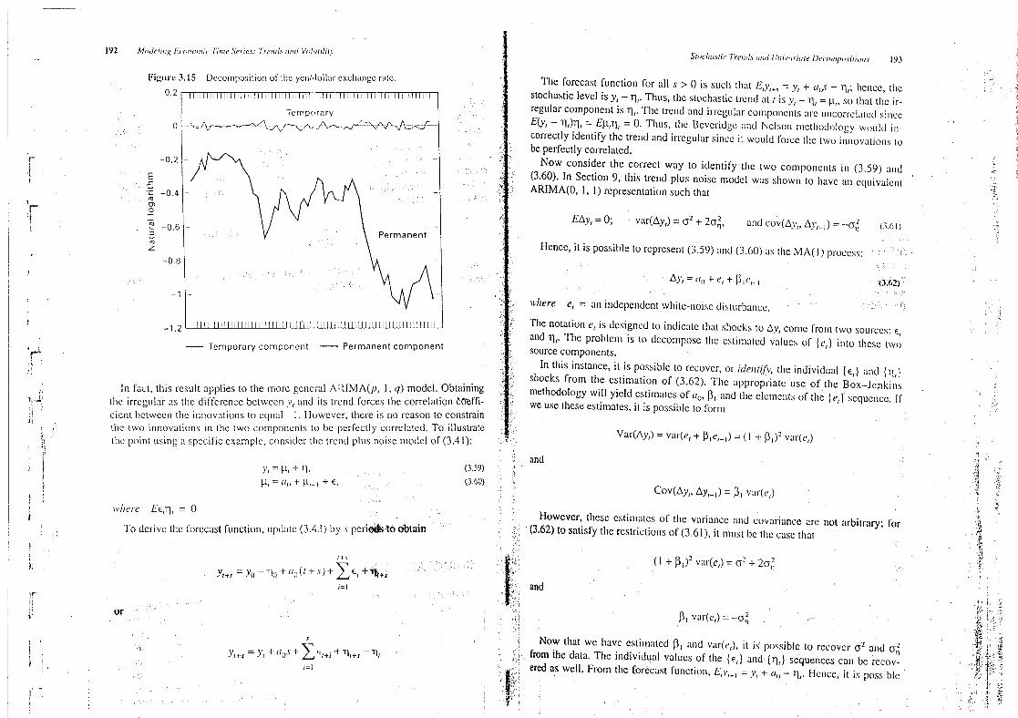
?f.-.ttit

192

In fatrt. tllis result applies to the mortz gcnccal A ;tIMA(p, 1. q) modcl. Obtainingtllc irregula? as thc diftkrencc bctwcen y, and its trend forces the corrclation tffi-cicnt bctwccl) the illllovatiolls to etltlal -- 1. l'lowcvcr, tllcre is no reason to constrainthe two innovations in thc two compollents to be pcrfectly corrclated. To illustratctile point using a specic example. ctlnsitlcr tllc trtrlld plus noisc lltodel of-(3.41li.

Tlle forccast functioll for all s > () is sucll tllat Etytn = y, + (lv - 11,., hcllcc, tllcstochasticIevcl is yt -

nt.Thus, tllc stochastic trcnd at t is y - q, = g,. so tllat tllc ir-regularcolnponent is n,.Tlle trcnd and irregtllar conlponcnts arc ullcorrelatetl si llccE', -

'n)'f),

= f'yt,'n; = 0. Thtls, thc Bcvcritlgc antl Nclson Ilctllodlllogy wtltlld i!)-correctlyidentify thc, trend nd irregular sincc it would forcc thc two innovations tobeperfectly correlatcd.

Now. consider thc correct way to identify' tlle two componcllts in (3.59) alld(3.60).In Section 9, this trcnd plus noisc model was shown to havc al) cquivalcntARINIAIO.1, l ) rcpresentation such that

E y = 0; vartAy = c2 + 2c2n' 2and covttpf, A)',-j ) =-clj

l10l1C0, it is POSSiUIC to I'CPIXSCIIt (3.59)and (3.60)

as thc MA( 1) proccss :' '

' '? i7' ' i '

l

w/lere etThe notation c, is designed to indicatc tllat sllocks to Ay, comc l'rolll two sources: 6.,and nI. Thc problcm is lo dccomposc. thc cstilnated valucs r (et ) into thcsc twf)Source componcnts.

In this instance, it is possiblc to recover. or idelllify thc individual (Ef ) and lrtrJshocks from the cstimation of (3.62). -I-llc appropriatc use of tlle Box-lcnkillsmethodology will yicld cstimates of (70. j)land thc elclncnts of the let )'scquencc. Ifwe usc these estimates, it is possible lo forln

= an illdcpcndcllt wllitc-jloisc disttlleballcc.

VartAy' = vartt,f + jl et. j ) = ( l + f'J: )2va1'to)

and

Howevcr. thesc estinlatcs of tll variane and covariance arc not arbitrary-. for' (3.62)to satisl thc rcstrictions of (3.6l), it lnust bc tllc casc that '

(l + j$1)2va4c,) = (7.2 + 20.,21

and

@j'J vart ctj =

-(y,2

k l

Now tllat wc llavc estilllatcd f)I alld vltrtcr), it is Ilossiblc to rccovcrc2 alld cyjE .. ' '' '

..from thc data. The. individpal valucs of the (E, ) and (n,) scqucnccs can be recov-;

. . . :.ercd as well. Frol'n tllc fbrcast fbnctilln, l.Ltvt.t =

.#,

+ (lft -

n,.Hcllc, it is possiblc. '

, ,

.

t'

tt .

xySttllttttll.j' (??!f y fj.tlttf.ttt.vi;ttt.j.

tk) tlsc ollc-stcl) :l1)c;ltl tbrccllsts fronl (3.62) to I'il1d EfA.y/.1 = (J() + kJl et. so tllat nd (3.54)with ja =--tllc

rcscarchcr wi1l set the irrcgular conlpojlcnt cqtlltl lo-jj/r,,$.,.j = ),, + f?(j + j j c,,. sincc thc two forcc:tsts ! tlust be equ ivalcnt. it follows that i .

, n'lultiplicd by thc ea tirc innovatioa in y, (j.c

., q, + q,). jq jn j-ac (, tjlc jjaylokatiollsarc

tjn cjlry'gjatg tjy(;a(;ttjtjj y tjj jj (y oj (jj jy yajyjj jj jtjy. jj j y jy yj o ymjyjyyjyjyyjy j js yj yy jj; yjj jyjyyysjyjyj

jo x

.,yj

y

y

jj o ys yjy jo yjy jyjy jyyy j j;jy, y

jm jyy ,

moyjjyj jj yyjs y yyjm jajyy jj yyjyj/1 /

W t5O 11 (1986) decom pos ()s the 1og ari tl1In o f'

GNP'

unde ;. tj)c tw o a1tcrj1a tivc ;ts -

Tjj u j y j jj(y (; j; (jyjjjj ((;(j va ju t;j o j* jjj gy (;kj jj (.): jj j; (y( j (() j(.j(;jj( j j'y (jj g g jj (j j.; (g j j gg. . y jj mjjjjou y ooujyjsu jyjy j jjy yjyyjosyj j joyyy yj.j j jyo jysyy jy yjyyy.y yjsjyy jy ja s syyyyyjy yy yyyysjyy.yayyjy( jtjcjlcc. G ivcn (ct ) and (T)/ ) . tlle vltltlcs O 1-(6., hcall be obtaincd froln A.yl= tl() + t + and Nelson decomposition, he estilnatcs tlle ARIMAIl , 1, 0) fllokjcl (wjtl) stlatlardZ1)/. For oacll valtle Of J, Forln q.t = AA',- t'( )

- 2'.11, usi n g the known valucs of Ayt and errors in parenthesesl:tllc estilllatod Values Of tJo and A1)/. ' '

Thc point is that it is possible to decompose a scries such that the corrclation bc- tjyt = 0.005 + 0.406A)7 j + zt, (y .(;.()j

()...ytwc.n the trcnd and irregultr componcnts is 7.cro. The example illustrates an espc- .. ,-

. (4,.(sj ; jyj.jp-yjCilllly important point. TO dccomposc a scrics into a rantlom walk plus drift and sta-tkonary irrcgular conponent, it is neccssary to spccify the correlation coefficicnt t . Assumng that jnnovatjons in thc trcjld alld irregular compoant: jtt. jjjjtottobctwccn innovations in the trend and irreglllar compononts. We 11aVC Sccn tW0 :41: '

jatedy Watson estimates yt = g, + z(/.)qy..22

;'

.q.

.'

;!ways to dccomposc :11) AItlMA(0, 1. l) moklcl. ll1 tcrms of (3.59)and (3.60),thc ttr '

Bcvcridgc and Nelson techniquc adds the rcsttictioll that '.

,,:

ujt .() (sy o jg o..(; ts.y.y. . t .

y. .. ..

. I > .

; :. .,. . .... j.: ..

... g'. .a

'h!..)jj ,

.!tjE '

c.6.qyo.c = l k.. '

,

',. (0.001)

? n y, y , ,, r;

,g rh ztz.ly).(j .j srljy-.j. () s-y-yy-zl,j o..(;

tj(;-yty($ z .

.

i . tn

l hc innovations arc pcrfkctly corrclatcd whilc thc second' decompsitih-' '

(0.121). (0 I25)'' '

S(J t 1at t . t .

).

adds tllc rcstriction-. qt '

.t.b't The short-tenu forccasts of tlle two nlodcls arc quile silplijar. Tjle standard-error.7.'. cf the one-stcp ahcad forecast of (l)9s sccond nlodcl is slghtly smallcr than that of-i 7

:'.);i.tc rst: (c2 + c2) 1r2

o () (0j).4 js sjgjytjy sjlyajjtx than ().: l(s uowcvcrthc Iong-! ;'.

*.1' 2.1*1 '

ln fact, the corrclation coegcient bctwecl, the two componcnts can be anyuum- .j' :'BD Properties of thc two models arc qujte dij-fcrent. I7or cxa'mplc, wriling

z,.j, =,p (000..,5+ 6 )/(j - ()44y)4$/.)yjejr-js tjjtj jmpujse response function using tlle ucvcrid'ber in the interval

-1

to + l . Without the extl kl rcstriction concerning thc correlation 'Ltj -

: .

. y antj xejsondecomposition Thc sum of the cocfficicnts for thfs nlptllscrcsponvolnctwccl!the innovations. the trend antl statilhna:'y components cannot be identificd; .t. .).

,. .

;k . function is I.68.

Hencc, a onc-unit inllovatioa will cvcntually fncrcsc 1og GxpbS0il1a scllsc, wc arc an cquation short. This l'csult carries ovcr to more complicatcd q. 1::.

tvltraszc',ortqpartition'' the contemporancous 7'kut' 2 fD11 1

.68

units. sincealI coefficients arc positive, followng thc nital sllock, Jmodclssince it is always nccessary to c :rj :., stcadily jncreascs to its new level In contrast thc sccond snodcl acts as J'lnovcmcntof a scrics into its two constitucnt parts. The problem is important bc- rr . )t .

cj, ,. RIMA(o, j 2) sucj) tllat tllc sum of the impulsc Jspojlsccoefficicnts is only0.5-11causc ccollomic thcory docs not always providc the rclationship bctwcen thc two ,.

. yJ ,

''.,r' 11cocfficients bcgnning with jag 4 are ncgative. As such a onc-unit inTlovaticn in'illnovations.Howcvcr, withou: a priori lpztnv/czjc of fc relationthp between in- ' ).., )..;

! .4 #: y as a Iarger effkct in the short rua than tht, lollg I-ulp.

'ttovatiots F?)tlte Jrc?zl t??lJ staionary co/uptlncp/l-, tlte decotnposition of a series ; g t'

,..y

r rj'?7lo tl

rtlt'lfltltt

T%?tt/1 illu- drtf: t1?'lJ(1 xlfl/ftallflry

cf?/l?/'7t4?lc?l/'

i'.s'not lt/lif/l-lc. '

. J ! ..j.. VL,Li '. yt

. .

What if 6, and n, arc nncorrclated, btll you inorrcctly use :! Bcveridge nli (,7''i. i.

l ': SUMMARY ANo coNcLusjoNs; ?pqr2;j

Nelson (1981)dccolnposition to obtaill thc tcmporary and permanent components ( :tk :k 4' ljst- .j-, .'1. 'Clearly, the in-snmplc fbrccasts arc illvarinnt to the form of the decompositloluj ?,.t: . :7 r: ytjty ;,uarlyeconomc tilne seres exhibit pcriods k)f vtjjati Ii(y. Cojlditionttlly jlctcro.

Equation (3.58) has an AI?-IMAIO.1, l) rtrpresentation that you should propcrly:F',* .

j .(.g, ) ujtjaujjcapturc using Step l of thc Bcvclidgc and lklclson metllod. As such. there is no Fayj. t - --. c jnodels (ARCH or GARCH) allow tlle coaditional varianc'c of- a serjcs to

' .

(.

l ! j.jl ;'

; j;r ; : k ..' f

.''

jjljrrifor yotl to dCtC1'1M if10 thllt th0 ZSSUIMPtiOl1 (1( PCf l 0CtlXCOW0z2tCu .11l1OV2t.Ol1w .S .D* tJ.li t ji P0Dd Ol1 the' Past rca) izntions of the error pnlccss. A Iargc realizaton of thc cur-. . j j g.j

.,!

j .j.

.corrcct. Tllc issue has nothing to do with 1l1e ctlrrect form of the ARIMA modell'.u4x

'(- rz-t Period s disturbancc incrcascs lhe condtiflnal varancc'in

sbsequcjlt pciods.i ..zi)

r jbr a stable proccss, the conditinal varfancc will cvcjltally dccay to thc. long-runrathcr, thc problcm is thc way in whicl) th'c innovtions in the trend and rregulai .

'

uj).?.

-

. i ( jts arc pal'titioncd. l !.'3)'.

f' .Ctmditional) variancc. As stlch, ARCI.I tlnd cajycj.jIuotlcis can apttjrc pcrlods

componcn r z 1 ,

' .../.p. ,,'

f ttlrbtllcncc and tranquflity. erje

ljasic GA acpl modc'l jlas bcca cztended jyNvhat will thc rcscarclacr i '

kcorrcctly pllrtitiolling thc varianccs Gnd? Using .'i..). ii'0 i

g.;,y

y y..s jjy yyyyyynoyyjyysyosj yyyyyyjo ayyow yyr yy jyyyjyrooy yyyyyyosyyoyyjjyjyoyyzj syyryyyyyjm.,

Bcvcridgc and Nclson tlcconljosition for 1tn ARIMAIO. 1. 1) model scc (3.42)'rs

j, S,

.:()

...

.,

j .

..; :.

'! : lt' !'

.t,..?;:,. ;)j..

.7%:. ..)(

j;:,E.

7:..'gg(tj!.tr .. q..''j.z'

.1

.:L' .

:. ' '; J. '..EC. . .

.i.. .. . .

..

.s; . gy...

.. .

.'' .g r

'

. .

. .

.

'

)' n :t .

y, = y,-1 + 6, + 0.5E,-) ),, = 1. 1y,- I + 6, '. L . . , ? .

..

.?r, ?,.'

p.

E):(.;:.') ,)7;j.

'... ''.

$7I DZ: )lt- 1 -B -/ ts'. J@t J?/- 1 : yN

'

.

- t#. yj y

).@ .

.

v kj = r..;,.;j,.l' .,r k ). .A '

.'

..g,.. . jy'' .k

ti. jr,

,;. t). ,

i' ')'''z.. .

. (r! '.)

2.i.f'''.!$. L'itl;'6,'

'zr:q

'

.

t.''

: .f):(:,., .E:

.:

?.. . .

.

.t'a :1

.r:j) :k.

.

,,

. . t .:'ti-'

'. .

.i'?, ..;;

.,I:,?t sj. ,

.1,t =

k:L''i.T'.

.*5

...i tjk..et.t ? .

.C?.)C.

. . (..( jslodcl 1: y, = 0.5.y,-l + e,

E')):))), t+t.t.#' ?t;j.$i''

! '.1.)

u jNlodcl 2: yt = zt - E)-

j

.' Lrjjp kt ,4

idt;.4 ;:,7?J.iNlodel 3: yt = 0.5 ,,-y

..1.

et - E2:-I ; k,.ij. Tkt.j

- j ;,...yjxtrtkj

'.t,...r .769,j.lt.

j ti,i.. (...A. How docs the ARCH-M specification affoct thc behavior of the (y,)sc.- l ,, j y;1.

. j-:r.

jy..; .quence? What is the influcnce of the autoregressive term in model 32 .): tjjy!5 '

y .!!'tt y l #.lB. For cach of thc thrcc modcls, calculate the sample mean and vriance of i

''f.,k.s

i )r. zij.

. ..J ti.(.J',)-

.'

'.;s til.

( r',?'z) i

. (.;j tjzyh;kt.

jjy .

6. Thc filc labeled ARCH-SVK l contains tlle 1OOrealizations of the simulated (?j. wazk'..

6..* ::. .

t' ?'k'tljjkr!7

(y,) scquence used to create the lower right-hand graph of Figure 3.9. Recall : i.

..il ?j.9'

that tllis series was simulated as y, = 0.9y,-) + %,where t is the ARCHII) dnor E . : .

.auzr

1/2 '' '1)fk

.16!5t'

process .t = v,( l + 0.8e,-I). You should tind that the series has a mean of (s?.;' t''.

. ..

jqdi;,':t:'.

.' ;kyr),$.:,.

.

:;.:.:4:7:k!j2.'.'t)'

.

0.263369480, a standard deviaton ot- 4.89409 139 with minimum and maxi- ,. t.

. .r,tk..

#.,mum values of - 10.8 and 15. I5, respectivcly. ;(: ,

j.!F,it . :1..2-

.7:y.',: i?';-1..A. Estimatc thc scries using OLS and savc thc rcsiduals. You should obtain 'Lf')

j.),.,t!,

z...t.,y.

..'F'

y.IE,.:lj.

..'

(gijkd

k,,..

..j,.' ,tu ?/L.yt = 0.9444053245y,-1 + qt .,(tjt, At.-''

,2t1. u

Thc J-statistic for :71 is 26.50647. . . ,.

'

t. r.

.

Notc that the estimatcd value of- a 1 diffrs l'rom thc thcoretical k-alue of 0.9.,./.

.

't'

.

)...%

This is due to nothing lnorc than sampling en-or; the simulatcd 'valtles of (vl)'t2N

., i.

:...

. titdo not prccisely confonn to the thcorctical distribution. Howevcr, can you Ilr()-

:7:.:.

) y,xivl'.' 1.

.: rvidc an intuitive cxplanation of wlly positivc serial correlation in the (v,) Sc-

't'..)

-. Aji)t? ;

tlucllcc n'ight shift thc cstimate of t? j upward in small samples? 4', sCt k.

' ' ('B. Plot the ACI7and PACI: of the rcsidtlals. t'se Llung-Box Q-statisticsto dc- ';Ej:

-.

t'L'til'

'51'

tcnninewhethcr the rcsiduals npproximatc white noise. You should fintl .:;

t.

,.r.

j4 ?;.;);j. tt.

ztCF ofbe rc-t/atll-; .. j .

i. .

k 7.! .

>.).

0. 1489160 0.0044 l62-0,0178424

-0.0124788

0.0682729 0.*28705 'J% $

't(l* ' :-0.0994202

-0.

1508656 0.0643873 0. 1012332 0.0898023-0.03791

16 ,:j t'/5.$:i!- '...k

'.-.

..;.,,.jb.

;rj.:y,

.'; 'kgtk h$.:.

! '9. :4. .

PhCF of t/1esqlared rc.fJllcl'.-' 1: 0.4730473.

-().

l 248437-0.086

l060 ().()03798 ().l 35 l502 0. !98 !7 !(h7: 0.0702680 0.0620095 0.0682656

-0.0656655-0.038

l 7 17-().

l030398i.

t Ljung-Box Q-statistics:Q(4)= 25.4702, signicancc ltzvcl 0.0000123 !(2(8)= 45.2535. significancc lcvcl 0.00000012

! :(24) = 50.'6029, signilicance lcvcl 0.00076745

#.?tCI7 q/-J/lt.> r(.n'i(1l(lIs..1: 0. l489 l60

-().()

l8 l625 -0.0 I6 l 7 l 2 -().0()747 l3 ().()727 Izkt,l -().()

i920587 :

-0.0996379

-() . l234779 ().l l l 5448 (1.()73 l477 ().()('J()(39 l 3 -(J.()5(556()

Ljung-lsox Q-statistics: ?(4)= 2.3 142& siglti ficance lcvcl 0.50980859Q(8)= 6.386 1, significmlce level (.).49546069

Q(24)= 18.49 l4, significancc lcvcl 0.7303 1863

C. Plot the ACl7 antl PACP of tllc stluarcd residtlals. You should l-illll

z!CF of llte squared residtlals:

0.4730473 0. 1*268669 -0.0573466-4).0777808

0.()57t)6l 3 ().24240390.2727332 0.2 l 40628 0. 1368675

-().0053388 -().0660

I62-4).0942429

Vascdon tllc ACl7 ltnd PACF ()f tlle rcsiduals and sqtlal'cd rcsidullls. wllfttlcan you conclude about thc prescllce of AIICH crrors?

D. Estimate thc squarctl rcsiduals ts:62,

= tAl+ (y.1e2,..j . Yotl should vcri

StandartlCoemcient Estilnate Errer f-statistic siktlificallctt

txo !.5501077352

0. 54849064 16 2.826 13 0.0()573246ct! 0.47450954 18 (. )899397 l 19 5.27586 ().0000()082

Show that tile Lagrange multiplier ARCl-IIl) crrors is TS2 = 22,()2777 ! witll 'a.significanc.e level of 0.00000269.

E. For comparison purposcs. estilnate tltc squarcd rcsitluals as aI) A1lCHI4)process.You shoald 5nd

StandardCocmcicnt Estmatc Error d-statistic ' Significallce

ct() l.934317326

0,65378 1567 2.95866 0.00394756al 0.520622481 0. 105584787 4.91085 0.00000372az

-0.079036621

().118547940-0.66671

0.50666555(yo

-0.089

l27597 U.! !8593767-0..75

!54 0.4542,036(x 0 0048 l259) () l05446847 0.0456:1 0.983698274 .

..

'j .

. '.'. .

t'7* ' '' '

Sfln u 1la1)co u,s?y cst iJn atc !hc )': ) sc t; 1Jcn t-c an d A RCl1(1) error' Pt6t'.t bs-

iI1g 111ttx i1)) tl 1,1.1likc lil'lood cst i11'1:1titn . Yotl shotl Id fi l1d '

EE . E..

7

StalltlardCoeflicient Estinlate Erl'or f-statistic Significance

0.8864631666 0.02707623 12 32.78797 0.00000000I

+l 1. 1735726519 0.2703953538 4.3402 l 0.000014231

(y.l 0.6663896955 0.2221985284 2.99907 0.00270202

- .)') jusalc pricc7. 7 hc file WPI.WK l contains tllc tluartc) ly valucs of the U.S. W o

Indcx (WPI) from 1960:0 1 to 1992:92. Usc Chc't1i:

ta to construct thc logarith-micclpange as .

IACF

1: 0.0 l 15085 0.03 15 14 l

7: 0.0369360-0.065987

l

',i. '.'( '

Ljung-Box Q-statistics:Q(4)= 6.2 l 72, sigllificance lcvel 0. l 8350 14)4'i

'

Qt12) = 3 l.5695,

signicancc lcvcl (J.() l ()l t9()Q(24)= 49.8 l 18. signilicancc lcvcl ().()()l496 I 1

-().0727560-0.

l6 l 6008 7.().3873 l 24

().1446746-0.082

l942-0.()05

l 1()l

B. Estimatc the (y,)sequcnce usillg tllc Box-lcnkins mctllodlllogy. 'I'ry to iI1-

proveon the motlcl:

.J'l= tJ() + EJ + f'$.$E?-.:5+ k1$f,E,--(,' '

. ,' E

..E .E ,

'i''

''. : '

''

You should lind: :.( E

ObserYa- StalldardSerics tiolls Mcayl Error Milzimum Maximunl

wpi 130 65.09 3 l.366

30.50 l 16.2

Llwpi 129 0.0 10 l428 0.0 I :152535 -0.02087032

0.06952606 '

A. Use the cntire sanlplc periotl to esti Illate Equation (3.19). Perfbrlrl diagnos-tic cllecks to dctcrmillfz whethcr tllc l'csiduals appcar to be white-noisc.

B. Plot thtz ACF and PACI7 of thc squarod residuals.

Estimkttc thc various GARCI-I nlodcls given by (3.21). (3.22),and (3.23).

whcrc

Stalldardi t Estimat Error f-statistic SignilicanceCoefl'ic en

ll 1.07 177108 1 0.048009924 22.32395 0.00000000% 0.254214138 0.098929960 2.56964 0.01 170287

%-0.262006589

0.099273537-2.63924

0.009682 !4.' .,

i' .'

isyV.Examinc the ACF and PACF of tllc rcsiduals Ikom the MAt(3, 6)) nloklclabove. Why might someone concludc lhat thc rcsiduals appcar to be whitc-noise? Now cx:tlnine tbc ACF alld PACF of lhc squaed rcsidtlals. Yousbouldtsnd

z'tCF of J/lt? sqllat-ed rc-$''JI/fz/'.'

1: 0.498 1203 0.2569847 0.289597 l 0. 1625 l92 0.04309887: 0.0907499 0.()532747 0. l 365066 0.026 l 8 14 0. l 592 I52 0.25()3244)

PA CF oflle 'fytffsrcr residuals:

0.498 1203 0,0038049 0.2 170029 -0.0878890-0.04

l 3535 0. l 01j6720 0 172378 0.03482 i 3. 0.0984692

-0.

l475 l0 l 0.2890676 0.0321684

Sanlplc nlcan l.06988500000

Variaucc 0.267006Skewncss 0.47442 Significallce lcvel (Sk = 0) 0.05642422

Ljung-Box (hstatistics:Q(4)= 43.7460, ' l'7 signicallcq lcvcl 0.000()Q(8)= 46.5766,

. t significance lcvcl 0.0000(.?(l2) = 58.9 I 13,. significance levcl 0.0000

f.'') . t .

.

'

t')!' ..

2;.. .. ). .) t

. (j(J,4) uuz 64.5293

,. qign ificance level 0.0000

0.0 l l 5085 0,031 (3424 0.232004t ) -().0643045-0.

1395873-0.3094448

-0.0009952-0.

!573020 -0.2247642 0.1 86 l90 l-0.05

10400 0.045 l368

/:ltzz l() 4- (1 1 lt CF t

/, = (y. + (y.ld,t f) l --

q$: '

..i''.;'

:!(#;! /k?()(1 elit:J) fzrt??;:)??,itrhilt

e itprittt(..Trc?lt?.jtttttl /t//flll lil .

k.'b:;

. .'

Yotl s l1( )l1 ld j-il1d :)

t

1'

l 1 :1 l ...

t. ..

Cocmcittnt Estilnlttc ltlrnkr f-statistic Significance k:.- . . j ' j

aft 0.908 1809340 0.0646439764 14.04896 0.00000000. .

.,.;y

.....: Lq.Jy;

a, 0.6252387 17 1 0.349 1817 146 1.79058

0.07336030 : .

.. t

. ty. j..'jcxl 0.1079 17055 l 0.0 l 93136878 5.58759 0.00000002 .

) :

. .. l

. '.:..

. 57;' 1.

!.' E

ctl 0.597379 1022 0.2387 112973 ) 2.50252 0.01 233 137 kf t.:j ' ..

i: ..

E. Check tllc ACF and PACF of thc estilllatcd tE,) seqnence. Do they appcar.,1' .!i

:

..j''i.

to bc satisfactory? Experimcnt with several othcr simple formulations' of 9t)i!

theARCH-M proccss.'ii

.

'Y''.j.7.f'

yjt

9. Considcr thc ARCl1(2) proccss El: = ctj)d a!E.2j-j + ty,ze.zf.-,z. qy..r

r.,(,j( .

A. Suppose that y, = c?o + &!y,-! + E!. Fi j)d the conditional and unconditional ' i.'

.:? ;

.variancc of (y?) in tcrms of of thc par:llnctcrs tzl, %, al . and az. t:,ag;):.!

k. sjj!'..

;t.i ;'z.B. Suppose that (yt) is an ARCH-M proccss such tbat the lcvel of yt is posi- ,! !.w,..h !! ..

tivclyrclated to its own conditional vafiancc. For simplicity, 1ety, = w,+.

'.t'. jt

2 2 Trace out the impulse responsc function of (y,) to an,?)''

$(,lel-.! + aaEl-z + E?. .

! #'(E,) shock. You may assume that thc systcm has been in long-nm equilib- '.

cr..

. ji.:;-r,rium(6,-c= E/-l = 0) but now ej = 1 .

-l-hus.

tbc issue is to i5nd the valucs of ,t '

,.:

(s x4t..t

y!,yz%)?z,and yz givcn that Ea = E3 = .-. = 0. j'..th s

.v . j.y- t;C. Usc your answer to part B to explain thc following rcsult. A student esti- tr ?j,,

matcd (y,)as an MA(2) proccss and fountl tlle residuals to be white-noise. ..1.-.

A sccontl student estimnted the samc scrics as the ARCH-M process yt =%E

.2$

,1'.

.vt j.

+ (y. + ovz + E . whynlight both estimatcs appear resonable? How y.'' '.';'

! ! -- ! t--:! l ....?,

. 7

wouldyou decide which is tllc better lnodel? L),'. '..

.jk;y''

' y yjln gcncral, explain why an ARCH-M model might appcar to bc a moving f). s.

,' p.avcragc proccss.

,''' @. ) ji.f ,

2.

,:

('

41(). Givel tlle initial conditioll y(). find tlle gcllcl'ltl solution and fbrccast function .).'

tk?.

.:;tv- -::.

fltr tllc fbllowillg variants of tllc trclld pltls irrcgtllar lnodcl: '';.. :'') .

' .

.#' k: sy

.z

,)..

tlt #t'.(F 4.t Kr.B . yt = t, + v/, wllcrc lz, = llt- j + 6, :1I)d 1', = ( I + ) ICl'r)t and thc correlation 1x- '..t

y.(.l ls unity. tc l'.ki.twtlttll E 3n 1), Cfjtltl )/ e

..

.),..h;.

Finti thc ARIMA rcprcscntation of catrl. model. /1. ''?'

.5 . ..!k ?.

11 Thc columns in tllc filc labclcd EXRATIS.W K1 contnin exchange rntc indicrs i.jli.

..t))

.

k ltalian lira, C:madilmdollv. .

.'i,t''

Fk:for thc British pound, Frlmch franc. Genhlan mar . -. s'.

&'g: t''''''

.

and Japnnese yen ovcr thc 1973:Q1to !f)90:Q4Pcriod. The units are currency . j., 2.';j ?E

. .) ;... tr ..I.

'

-ltk .

'.

i.',

. (j(..$;

.

...I '

.'''''i

pcr tJ-S . dol ltr alll.l tjlc val tlcs 11tve bec 11 ctll vel'tetl i1)1() iT)d ices sll c ll

197 i-.()

i = i.00

.

I7()rthc ycn a nd Clall td iall (.1() lI111' ((.rt) ll l l 11l ds 5 l.t1)ti (). l'es lcc (i%'t..lly) j' ( ) l l >,ltk ) t.t!t Ind thc follo'svi1'1g:

Observa- StandardSeries tions Mtan Error Minimunl MllxintlmYen 72 Q.6t561729t67 0.t 547 ! 136l74 0.34%tJQ()0QQQQ(.$.8,43!676)()t)()()Canadian

dollar 72 1. 16505638889 0. 12397561475 0.957 l63000()0 l.39

l 88 (0()()0()

Fonn the logarithmic change of each of thc two scrics.

B. Decomposc the yen/dollar cxchange ratc into its tcmporary and transitorycomponentsusing thc Bevcridge and Nclson (1981) dccomposition. Youshouldbe able to reprotlulx the results in the tcxt.

C. Detrend tbe logaritbm of thc Canatlian tlollar ttlenotedby y) by estimatingthe regression yt = ao + abt + E,. Savc tlle rcsiduals and form thc' corrclo-gram. You should find that the rcsitluals do not appcar to be stationary. I7orexample, the ACF of thc resduals is

,1CF ofthc rc-i//lfJz/'.'

1: 0.938 1 08 0.85 16773 0.7656438 0.6707062 0.5656608 ().46460907: 0.3665752 0.2619469 0 I602961 0.0668779

-0.02335()0-0.0959095

7

D. Estimate the Iogarithlnic change ln tlle Canadian dklllar as an MA( 1) modcl.You should find

hyt = E( + 0.630867 l 509e,-:

The standarkl crror of j'sjis 0.092738 !095, yieltling a J-statistic of 6.80267.E. Perform the appropriatc diagnostic clccks of thc modcl. s it necessary to

incl ude a con s tant ? Wh :1t abou t thc a u toc orre 1ati on c oe ffic ic n t o f0.2249136at 1ag 3:?You sh luld verify that tllc Ljung-Bix Q-statisticsarc:

Q(4)= 5.6965,Q(8)= 7.9077,

(?(t6)= 16.3652,

sigllificance level ol-0. 12734706significallcc lcvcl of 0.34080750signifieance leve.lof 0.35820258

F. To keep the issuc as simple as possible, procccd with tllc Bcveridge :*. d.Nelson decomposition using'th MA( l ) modcl. For ech period t. fofm thtvarious

--stcp

ahcad forccasts. Why ij it stlfficcnt to 'sct . = 1? '

(' >

..2.

!..(.) .. jrj

f .( ( .

?.

7()4 ; .t , , ,

:k t . .,

. ) .

.,) .z

G. Forn) tllc lrend Jnd irrcgplar colnptlllcllts of tllc logaritm of lhc Canadian j ?'t idcntical samplc pcriod. ll) (llis way, lllc nuTnber of usable obscrvatiolls wil) 1)citlcnlica), .

'' .$ fo/tbe two models. In this scction, alI models werc estinlated over thc I962.2 to 1992:2dotlar. Ytu sllould bc ablc t vcrify' ' ' '

'2..@ .

',>K .':

sample period. One observalion was Iost duc to differcllcing and cight werc lost duc to'. :

.'

.).

. thc cstimalion of thc ARCH(8) modcl.Trend Tmnporary ;$.xy.(. .

7. Tlyccstillatcd valuc of /I, s the collditiollal variancc of- tllc jogarititlllic changc in tllcPcriod lyog CanadiJtn $ Conllltlnellt Conlponent ..r( f

.: WPI; in constructing the figurc. the illtcrval for lllc pcrccntagc challge was convcrted torv 2

1973:02-0.008634167376

-0.006909245096-0.00

1724922281 ( p tkc level of tlw wPl.

,9,3..0a-().()()4ts1s9to:z

-(,.(.03260-,.26492,-().()()l411.,f)9s4() .'?

. s. In adklition to thc iruercept teou. orc.eseasonal uululnyvariaues werc alko iwluaca i,,

.,..

the supply equauon.l973..04

-0.008734030846 -0.0

l2 187 148030 0.0034531 17184'j

::

.7j..gt 9. lf the undcrlying data-gencrating process is aulorcgrcssivc, adaplivc cxpcctatillns ltnd ra-) - 7

) i. tional expcctations can bc pcrfectly consistcnt with cach othcr.. ( '

:'

..

'

.; ;. ..

'

1.:'

:'

I990..03 7 0. l34045635379 0. l 32362802801 0.001632832573,)

,'. 10. lf the utility function is quadratic and/or (llc cxccss rcturns frolll hofdiny tllc assct arc.. .

.. t ,,

9...,:.:4.o.t4escl3s()..)-'z ().l4(l5'?($?.(o84-0.005336239112

't.

b normally distributct,, a increasc ia the variancc orreturns iscquivalcnt toan incrcasc ,'l . ;.2i..... .$ yq j lr y,.

.:)

' ..J 1l . Of'coursc. to thc individual contcjnplatillg thc Ilurcllasc or a risky assct. thc vuluc of g,11. j-low wou ld ytlt-lstllcct .$' if you fptlnd tbc atllorcgrcssivc cocf ficient at lag 3 .j?

j jyastjc. xotetjyatjt, is tllc cxpcctcd rclllrrl that thc intlividual would dcmand inE : ) s not stoc!O be im I)O rtarlt

'?'

1.,.. jt order to hold thc long-term asset.

?' t 12 'rhe

unconditional mean of y, is altcrcd by changing only 6. Changing kJand commcn-1. Dctrcnd at least one of tlle othcr exchallge I'ate series in the lc (youmay (.t -..j -

799.t surately maintains the mean valuc of thc (yp)sequcncc.co n v c r ( t Iogs ) . D oc s th c dct re nded scl' ies appea r to be s ta ti O llary 'h '' g?:iy'

-i;

l3. 'l'lei

Greek tharacter set and' subscripts deccntling below lle line are not pcnnittcd inCompalc with thc lirst diftkncncc of the serics.

'j

..).j

jjwvs. vo actually write sucb a prograln, the paranletcrs jJ. (xj), c,l, antl 7,, migllt be tte-.

. .. it--,...

.. .-.,,.,

.

..q: 7

, r noted by B, z0, z, 1, and zaftp.rcspectivcly. '

, .r. ,, ,,.

,..t!

: j4. 'I''hemcthod is recursive since the prograln first calculatcs E,, tllcn /),, and thcn LIKELI-(4 ;

jyuopENDNOTES '., ;

.

t! . l5. In actuality, the program stcps in RATS would diffcr slightly sincc e could not be de-rt . fined in tcnns ot- its Own lagged valucs. Sildlilar rclllarks hold for aI1tllc progranl slalc-

1 . Some au thors prcfcr thc spcl Iing llolllosccdastic and hcteroscedastic; botl) forms are cor- t.rlt' (.) J . mcnts below.Kct. .

* '*-h'

q;?1

j', v .

i'i : l;. Many treatments use tllc rcpresentation yy = trcnd + cyclical + scasonal + inegular. In2 1f thc uncondi ti onal v ari ancc of a scrics is not constltnt. the serics is nonstationary. ijj $'' lj y. tjje tjixy any cyclical colnponents are includetl witll thc incgular tcrnl; thc notiol! is tllat

il Owevcr, condiIional hctcroskedast icy is no: a sotl rce of nonstationari ty...6stt ' '

';: ' . c clical economic compotTents are Ilot dctermillistic.i t() ;'l ; i11 t111t! .'.;ij.y'k''61..1 lf3. Lctting a(J.) alld j(L) bc polynonlials in the 1ag opcrator L, we can rewr

:.;,j..js l7. A linguist might want to know wlly ''tlctrending''

entails renloving the dcterministicfonn:

.),(

.T-t. j; .

trend and not the stoclhastic trend. The rcason is purcly historical'. originally. rcnds werc. . .

!;J Iidr ..

c'if './;J viewc.d as dctenministic. Totlay. subtracting 111e dcterlllinistic timc Ircnd is still c:tllctl2 / ?

'''1*

Itt = .jl + kllujef + 11()1,-1 j.j s'ry qljjrjytlyutjkjygs,,

.k. ljtt;' Lj1.

,t.:'.

18. lf Bl is of in fini (c order. it is assu nlcd that Zj-$/is finitc .

ejnhc notati On (,( 1) lonotes (he po1ynomi :t l (z(A) eval uated at L = 1-, that is,:j,1'

LLL'L1 lf only s(,) hps a unit root. the proccss is llot i1)vcrtible. -rllc

( ?, ) sctltlellcc is strttiol) llryjt: tjF.

j ) = a + (z + ... + (vy. Bo))crsl ev (1986 ) shllws t11at thc GARCH process s'''),''

.. . (maybe slationary). but tllc usual cs1i1.,3:,1i()l) lcc, llliqucs al'c illapprefll.iatc. I1.1.)()(1,zl(/.)CZ( I t .. .? . ..

.

stationarywith k, = 0, vartei) = L1 - (2t( l) - ;'J(1)1,and cov(f.?,E,-,) = 0 for qtq ..u'1,.' and Bl.j have unit roots. tllc colntltoll pl'/flr pnlblcm tliscusscd il1Cllaptcr 2 cxisls. 'I'11c'tilp n.1 unit root can be factoretl from A(f-) and BL). '

s #' 0 if (y.( l) + j( 1) < l . t-4 uszj

11of white-uoise errors versusi,,''-.- Tli,

2. EAlsc assumc that alI values of Ef arc icrofor i < l .4. Unfortunately, lilere is no available mcthotl to test the nu p.' ' ':' ?721 fAs

an excrcfse, provc that ihe first dirtkrence' of the tr'cld acts as a rartdom walk plus' thc spccific altcrnative of GAILCHIP, q4 trrors. Bollcrsltv (19%6)jfoves that the ACF; l'$<k.

', .

k ..' yq.... . .. v.,24 ;

.. .

of the squared rcsiduals resulting from (3.9)is an ARMAIm,/.)) model, where m=.) 1)-. 7j.: ydrift. Show that g, - g,-j hTls the interccpt tzo'plk!s a serially uncorrelatetl error.

. .k :F. ,

'.

. .

maxtp,q). Question3 asks you to illustrate this result. l tj yytl..:'22. 1'1-h: ssumption tllat t, ankt,n,

are uncorrelatzd places rcstrictions on tlle autoregrcssivcl '..lj n.

' >r.' ' : ' ' ' .

5. ctmstrainingthe coefcients or F?,to follow a gccayillg pallern conscrvcs degrecs of, :s VC..Iand

moving average cocfl icients of Ay,. I--orczamplc? iJ) lhe jurc random walk .plasl

d1,'. .)l-@'E 'noise moael, jJ, must be I,egative. To avo'kd'estijnating a constraincd ARIM'A modcl.frccdomand considerably cases tlle cstimation proccss. Moreover. the lagged coefii-' Ek.

;t .

E 't2 r7$ '

watsonestimates the trcna and irregular tcnns as unobservcd colnponcnts. Many soft-cienlsgiven by (9-i)/36(i.e.-8/36, 7/38, . . . , 1/36) are cach positivc and sum to unity. ; i.. ) I

t .71.,. . i.r'l' ''ware

packagcs are capable of estimating spch ctluations as tilc-varying paramctcr mod-6. Estilnating a modcl with n lags usually entails a loss of tbe tirst ?1 observations. To cor- , 4j,;j t: .p:...:.t'-.... . . .

tor this problem. thc Aaci.l ana oaacr.f lnodels suould ',e compared over the. '-..j.., &,k.:,,.1s.

ocfailsoftl,elroddurcan seos.--incdsnuar-y (Is8q). ,..

rec ,, -

,,..

, ,,.. . .

. 'el:

.. r .

ku ,'

iitk.4@r.

y,. j:, . .

.5 ;.(h yr t j .. tk )

i :r.L;.'.. -k .

..!ji

.)'

. . -

f ' '

E . .(

1 * e

j ;

1 .

l k

: D; j

i 1

k'

j .

.jt ;

r $..

'

w; ;

a.,$. t j ;);)c?: ($i.v.. ;fjtt, (: ! &.frt c fitlpj ftttf; gkjit,ittttttt yje ( ttxjyrjjjtj

re /g,yy)r,$ ijjj.yt.,

.t!, jj..

').

.

.

,w'.

.. ; E 2 ,

. : ' r'::

. j x ?q ; k'r .

q.;

,

,:

r i ,

APPENDIX'. Signal Exlraction and M*1hi+tlm., *4n,k:i

t,' , Sifltt, gx. qo. td are constants altd gx = E.., it follows thatS are Erro rs ' , . .

'''A'',. 1,.qu ,k yr .. k;.. :

'. ' .' ijjt.

j .( Ey = jtvLinear Least-squares Pro-jection '

'ir.

($ You should rccognizc this forlnula froln standard rcgrcssion analysis-, a regrcs-Thc problcm for thc cconomctric forccaster is t() selcct an optimal forecast of a ran- lrEj ,

. .'j

,, sion cquation is the minimum mcan square errr, lillcar, ullbiascd forccast of y*.dom variable y conditional on the obscrvation ot a sccond variable x. Since thc thc- 'j

. .;j..* ?q ne argumcnt easily generalizes forecasting y conditional on the obscrvation of thcory is quite gencral, for the time being we ignore time subscripts. Call this condi-

.;.$r i, n variables A'j through xn and forecasting y,+, conditional on the obscrvation ol- j',.tional forccast y*, so that the forccast crror is (..y- y+) and the mean square forecMt . j, i:, tjt t) yg-j,. . . . For cxamplc, if y? = a() + a lyf-j + E/, thc conditional forccast oj- y,+, iserror (MSE) Ey - y*) . One criterion used to compare forecast functions is tlu ,'j

k...'# . Et..k = av + ajyt. The forccasts qf yp+.scan be obtaincd using thc forccast runctitln'':MSE; the optimal forccast function is that with lhc smallest MSE. ..Ett a:

..k)j ,

s. ((skterativeforecasts) discussed in Section 11 of Chaptcr 2.Suppose .x and y arc Jointly distributed random variables with known distribu- .:4 -i

:1L ' '.'' !: '

'(''

.tions. Let the mcan and variancc of .x bc jlx and cz. respectively. Also suppose tlz ziik'..

,. ..

sjgnajExtractionltl(! bf .'r is obsclwcd bcforc having to predict y. A lnear forecast will be such that tQ' ' 'va .;

. y sjgnalcxtraction issues arisc when wc try to dccomposc a serics into its llldividual.,.j.

.

uk

thc forccast y* is a lincar function of x. Thc optimal forccast will ncccssarily be lin- ..'':-.

, r:

.yj y xcomponents.Suppose we obser've the rcalizations of a stationary scqucncc (yf) andcar if .x' and y arc lincarly rclatcd. and/or ir they are bivariatc normally distributel )'4.' .:.

hq'yj want to find the optimal prcdictor of its colnponcllts. lf wc phrasc thc problcm thisvariablcs. ln this tcxt. only lincar rclationships are considcrcd; hcnce, the optimal j.. : , , way, it is clear that thc decomposition can be perfonned using the minimum MSE-

,. .-, . ,- r .;.jjjr;;,tjgry!,torccast 01 ym n2s tnc ion41. j rjurjon discusscd bove. As an examplc of thc tcchniquc, considcr a scqucnce! 1) C

,. , yy v

'

, , . ?r (j f (wo irjde endent white-noise components.r . j(. :y, COmPOSC O p' * = a + bq.%'- P.)

.:

h.

'E

*

)? x.g.tj

')

yi .b..- (.:.i; , .

..

...; !rj(-,(t$ '..

j-.cr,:

.7) !(; wllere .l-Et = 0Eiqf ' q,

?,.t $ F E = ()qbis- '$

. 7:-1t.; ;

.. .

fkl kqt: .f'Et11, = 0,) r.: z z:gt'.?;t.

. E 6. = c;) t 6.

)E t; j.; .:E E 2

= 0.2lt; k ;,, p q, ntEs :( :2.tj., (Sincc E(.v- jta) = 0, Ey = g , E(.r - j1z)2= (y2, and E(&) - jtzjty = cOV(Iy yj = Cxyvijju.

'

$;) Herc the con-elation bctwcen thc innovati ons is assumed to bc cqual to zcro; it is.y x ,, y..t,l

2, ,

kt fo11ows that :*,1,.',1:

j htjbrward to al low nonzero values of EE q . The problcm is to tind thc opti malj (- .: ' !Stlz g-.

:?

- 4.2;. .r t

ijI..t'5:y.,'t

prcdiction,or forccast, of-q? (callede*,) conditionctl of thcobscrvation of-y,. Tllc lin-:#:2 2 2 yz rz - ztrzjj.- Ljyf;;). k.tj '.j.-f

rar srccasthas the forln.L2tu.y- y ) = Ey + a + (' v y xs j .(,eij:arj

lC, tcsh. ). :

?,qt '')7! i :l.

'a :j jtj; j jy jj:) y q:y m cj .j. yyMil1i miZi n %Vit11FCSPCC t to f.l llll d b y C j

'

j. $ ) t tt .4

lIa/. Jtk'

.: .

z (:) :( g). I tllis problcm. the intcrccpt tcrm a will bc zero, so that thc MSE can bc writtcn 'b = (5. /c . Iz'y A ! .y rtt.

j as;.k7r

v.r; .J. .t

o j,N

.. k jy- E

Thus.thc optimal prcdictionf.,rmula is ,..k ;j,'k z

., pf yxj.;. .,

,, .,. t,. ,MsE = c,(e, - 6.:.)

''i',,

,'

.'......

; .:. ))f .. = r-(e, - /py,)2

y+ = l - (cxy/czalg.r+ tc,vy/oQxl.x '

,,.j't''xzjf

,

s(e - yz, + rjyijc$j) tj. =

,

i,;x 6;1 . 1'

-*'.

.

Tllc. forccast is unbiased i11 the scnse that the mcan vaI uc of the forecast is :tlal jk l.j. Hence the opti mi zation problcm is to selct 1.1so as to n1in imi z :.yt .khc mcan Valuc of y. Take tlle expected valuc of y* to obtain s? ''

to t .(

y.ur ?.'.73 zt Msj;. az sj( j - yjet

.j)q

yy2. .

'. '. .... ..ltjklttq':'

k'Ilt : = (1 - bjljj..62 + bzggq2 sj jlcc k yj = Oj',.'h,

,?. . I t t tj ' .

, . . . . .

' : r' '

.;!!' ?

.'.

L

:?*.,If$i. r

208 $1(2(1e /lW# f)?;t)J?1 ic I'ime Jcr'e..' Frt'?l'Xutl(I Vfpltllflir.F..*y 2.

.yj y,

y ggpcygyj syyyyyjyy Exyssoysyyyqjvj syjysyyymyjgyy yyjyjy.o smyym zjsit, ,

.'/

y'Tllc rst-orucr

contlition is 'zj )'.' sinceajjopgscpr.. odjjctsarc zero, tjje problcjn is to sclect thc py so as to m in in)ize'p.jj'

. ).j . .. . . ..

.: ;q'E. . .:2!. kE!. ' ''('

'''

.'

.)

'-2 (1 - 1))t3' + 2:6,) = 0 ..ij'l. '...

.:

jA'

s' '.

..,$.

.,

'.

a ',). ..: ..

. .

.'.j i (l.j. : . E.L-

... f'rt: .

ob = C2/((J'2 + (J2) '..j '!

(n !''. . t! F.)r eRj,l valueof p:, the rst-order condi tion is. j tz t (Hcrc. b partitions y, in accordance witll the relative variancc of eg that is, c /(c2 L f.;j

.; . :

+ c2). As c2 becomes very large relative to cn2,b -+

1-,as 52 becomcs Mz.y small $1,.'i!

oo j1qI

;lLi-,. . .jt.$ -..

,lative to c2 b .-..y 0. Having cxtractcd E,, we see that tbe predicted value of n,i5 j 'q- 2cZp-2c2

1-

v. = ()twO innovations are uncorrclated. F V*.

r:.t 4.,

. l'>g.$ A11ty, j wilj satisfy tlle diffcrence equation givcn by (A3 3) To cllaoteriz: t&, '

t ., kForecasts of a Nonstationary Series Based on Observables ..2.k' .r:'

. .( yt natureof thc solution, ssct k = l , so that the rst cquation of (A3.3) isMuth (1960) considqrs the situation in which a researchc,r wants to finklthu optima!. zt: :.F,- u e

.forecast of yr conditional on the observed values of yr-j , y,-z, . . . . Let (y?)be a ran- .,$ 7. .:,:.J

?4 t'dom walk plus noisc. lf a1l rcalizations of (E, ) are zero for t S 0. the solution forh'k 'T.t 'x' i,k. '.t'-. $t..

:k42r,:;!: :E!: .js . i) jg ()' yj17j

- 2()' N 1-

vi = p..)#..''!/'

l,,).' .zt,y j = I i = jz /

.:' rt

J/y

. .. . J

).t q jfi'..)). $;.:.. and for k = 2.(1l) .

't

J..j.,..

..,j;... j..k$! iy

.:' ;: Ak';r. .:t.

.

t,rj./

; .

E'

.' :.

tii;. Fjq. 2c2 y, - 20.2 j - j, .(;w'/zcre yo is givcn and go = (). F .-..?.

,uj.

n 2 , ;.

. . $2

..

..- jy. k? E.:

.

.. tj.

j .2t = lLet tlle fbrccast of )?,be a 1incar functioll of the pwt v. lvt of th4 strivs, so that ;;.j- 'ttrftr

,gr7'). 'y%....

.gi.

. . . ' .. .. . .'k :r;.

..

z

. . ..LIL.;.. . . )?

. .. .

.;: 'k ..tj. f . . ' .(/!:;9

. :t)h' i'sjlj,..))r

'.':

v7;. . (.

.,. :):.

. . . .j;trry: ..

. jz .; mk'r. .

'..,.,jj$., .?:

l /j's.., . . t( . .

1)(2 V 1 r iOt ls Va1ucs o f T)j : rc s0 l()c ted s () as t() m inil'n izc thc mcan s uarei)'(. / 1' :L't, .

....t.jtk...:..7j$y

.-forcczst Crror. ' )j.uEj2'

-

v + j2 + (o.2/g2))v- p a (; gork az g g.: ,

... :-j : yj j k..j , , . . .

'utty y).

' /y',.' 'u!t!;

..'.Y-*j',/.'

The solution to this llomogeneous second-ordcr diffcrcnce cquation has thc form')'?.

. ).f )..) , . .

.x/i

k k.s,,krt.t

-.jpj=,>,

+ zktc-z, wlwre z, and xzare arbitrary constants aad 3., and .c thc charac-':k- 'zristic

roots. If you use the quadratic formula, you will find that the largcr root

'.'.

: .. :J$' .. $

. ' )t' ' .

.,. ':(uy, k) is greater than unity; Ilcnce, if the fyk)

scqucncc is to be.convergcnt. zglz. ;6:'t ez/-mtjstequal zcro. The slllallcr root satisfies.r' , k k

a..k'.t.?$ ..

',;)j

jy..

tk/ ) ! jq,t:j.

,Thus, tlle opti mization problcm is to sclcct tlle py so as to mini mize tllc MSE:,'',.j.,. '

494.. j.z - ja + Lazjgz)gj. .j.

j .(.)' jt/, :. :!) e n l

.: t .

-

. y ,%.*F * G'.

.L .Jt'.To tindthe value of z! substitute vj = zt j .y and fa = z4j l2j jnto (A3.4)..

. ..;jj .. .. rg .. j ,l T't:jtt'

.. j:

>:

.

' .y- .?7:.L;o>

.4.t;z; .r.'2

..)('L

. . , .j.. ..

..' , j .

k ii &

..

.. ...';.;L #y.' ) ..rk

. ; . ..' ;' JJy.j;.i.! .'.wts..jj ,

If you solve (A3.5) for .1

. it is possible to verify

A I= (1 - .1)/.I1-

Vt- .AA%'>..Q.A .Y

j - 1* 1 k.

. ? E' ''' C ' '

y: = ( - : ) l yt-j'

,

'( . . .y '. ..' (.(

''

. '(. ( y.. .. .

7=1

Since 1/.1I< l , the summation is such that (l - k,)skt-' = l . Hence. the optimal

forecastof y, can be formed as a geometlcally weighted average of the past realiza-

tionsof the series.

Uhapter 4

TESTING FOR TRENDS AND , rUNIT ROOTS

....

y.y.. t(.(y...j.-- -y.tj....,y..t.-.,....' '.

'.

r'

.( (.

S'

.

(E.'' (5 '.

Inspectionof the autocorrelation function serves as a rough indicator of whether atrend is present in a series. A slowly decaying ACF is indicative of a large charac-

.' t .).q. , . .,

telistic root. true unit root Process, Or trend stationary process. Fol7nal tests canE,yE.,

.; j ytl j jjeoer or not a system contains a trend and whether tat trend ist . jjelp determ ne w

detenninistic or stochastic. However, the existing tests have little power to distin-guish between near unit root and unit root processes. The aims of this chapter areto :

l . Develop and illustrate the Dickey-Fuller and augmented Dickey-Fuller tests forthe presence of a unit root. These tests can also bc used to help detect the pres-ence of a detenninistic trend. Phillips-perron tests, which entail less stringentrestrictions on the enor process, are illustrated.

2. Consider tests for unit roots in the presence of structural change. Structuralchange can complicate the tests for trends; a policy regime change can result ina structural break that makes an otherwise stationary series appear to be nonsta-tionary.

3. Illustrate a general procedure to determine whether or not a series contains a unit

' EE. root. Unit root tests are sensitive to the presence of detenninistic regressors,such as an intercept tenn or a deterministic time trend. As such, there is a so-phisticated set of procedures that can aid in the identication process. These

. procedures can be used if it is not known what detenninistic elements are part ofthe true data-generating process. It is important to be wary of te results fromsuch tests since (1) they all have low power to discriminate between a unit rootand near unit root process and (2) they may have used an inappropriate set of de-tenuinistic regressors. '

The Hodrick-prescott DecompositionAnother method of decomposing a series into a trend and stationary component hasbeen developed by Hodrick and Prescott (1984). Suppose you observe the values ylthrough yw and want to decompose the series into a trend (p.,)and stationary com-

ponenty, - gv. Consider the sum of squares , kt.

. . .r.. .. .. f'r).;.i.h

F F- 1

2 hl.) E(g.-p,

)-(p.,.--41.,-1 )j2(1/F) yt

-p.,)

+( ;+l t

= l t = 2

The problem is to select the lgJ) sequence so as to minimize tis sum of squares.In the minimization problem, , s an arbitrary constant reflecting the ''cost''

orpenalty of incorporating fluctuations into the eend. In many applications. includingHodrick and Prescott (1984)and Farmer (1993).k is set equal to 1600. Increasingthe value of k acts to

l'smooth out'' the trend. If k = 0, the sum of squares is mini-

mized when y, = gv',the trend is equal to y, itself. As k -+

co. the trend approaches alinear time trend. lntuitively. for large values of k, Hodrick-prescott decompositionforces the change in the trend (i.e.,Agr.l - Ag.,) to be as small as possible. This oc-

curs when the trend is linear.The benefit of the Hodrick-prescott decomposition is that it can extract the same

trend from a set of variables. For example, many real business cyele models indi-

cate that all variables will have the same stochastic trend. A Beveridge and Nelsondecomposition separately applied to each variable will not yield the same trend foreach.

H =i;E:E

E

....'

ar'

1. UNIT ROOT PROCESSES Thus, if tzj = I , the variance becomes infinitely large as t increses. Under the

. null hypotbesis, it is inappropiate to use classical stxatistical methods to estimateAs Shown in the last chapter. there are important differences betwecn stationary and and pefform significance tests on the coefficient t7l. lf the (yl)sequence is gener-nonstationary time series. Shocks to a stationary time series are necessarily tempo-rary',over time, the effects of the shocks will dissipate and the series will reverl toits long-run mean level. As such, long-term forecasts of a stationary series will con-verge to the unconditional mean of the series. To aid in identification, we know that

a covariance stationary series:

ated as in (4.2).it is simple to show that the OLS estimate of (4.1) will yield a bi-ased estimate of a l . ln Section 8 of the previus chapter, it was shown that the first-order autocorrelation eoefcient in a random walk model is

Pl = ((r - 1)/d0.5< 1

l . Exhibits mean reversion in that it fluctuates around a constant long-run mean.

2. Has a finite variance that is time-invariant.

3, Has a theoretical corrclogram that diminishes as 1ag length increases.

On the other hand, a nonstationary series necessarily has pennanent components.Tbe mean and/or valiance of a nonstationary seres are time-dependent. To aid inthe identification of a nonstationafy selies, we know that:

1. There is no long-run mean to which the series returns.

Since the estimate of t)j is directly related to the value of pj, the estimated valueof tzj is biased to be below its true value of tlnity. The estimated model will rnimicthat of a stationary AR(1) process with a near unit root. Hence, the usual stest can-not be used to test the hypotesis t7: = 1.

y Figure 4. l shows the sample correlogram for a simulated random walk process..

.. . ). '.'; .

..

'

.

' l. One hundred nonnally distributed random deviates were obtained so as to mimic

the (e, J sequence. Assuming yo = 0. we can calculate the next 1(K)values in the tyr)sequence as y, = y/-j + Et. This particular correlogram is characteristic of most sam-

?(: t ,,'',

. ( ple correlograms constnlcted from nonstationary data. The estimated value of pl is' l).E ,. close to unity and the sample autocorrelatons clie out slowly. If we did not know

the way in which te data were generated. inspection of Figure 4. 1 rnight lead us tofalsely conclude that the data were generated from a stationary process. With thisparticular data. estimates of an AR( 1) model with and without an intercept yield(standard errors are in parentheses):

R2 = 0.86

l

j

The variance is time-dependent and goes to infinity as time approaches infinity.

Theoretical autocon-elations do not decay but, in f'inite samples, the sample cor-relogram dies out slowly.

Although the properties of a sample correlogram are useful tools for detectingthe possible presence of unit roots, the method is necessarity imprecise. What mayappear as a unit root to one obselwermay appear as a stationary process to another.The problem is difficult because a near unit root process will have the same shapedACF as a unit root process. For example, the correlogram of a stationafy AR(1)

process such that g(l) = 0.99 will exhibit the type of gradual decay indicative of anonstationary process. To illustrate some of the issues involved, suppose that wekmowa series is generated from the following rst-order process:'

Fr = Jl)',-l + 6,

where(E,Jis generated from a white-noise process.First, suppose that we wish to test the null hypothesis that t2I = 0, Under the

maintainednull hypothesis of 471 = 0, we can estimate (4.1)using OLS. The factthat6, is a white-noise process and l(71 $< 1 guarantces that the ty,)sequence is

stationacand the estimate of tk! is efficient. Calculating the standard en'or of the

estimateof t2I, the researcher can use a stest to determine whether 471 is signifi-

cantlydifferent from zero.The situation is quite different if we want to test the hypothesis c l

= l . Now. un-

derthe null hypothesis, the (y,)sequence is generated by the nonstationary process:

Examining (4.3),a careful researcher would not be willing to dismiss the possi-bility of a unit root since the estimated valuc of tzj is only 1.5133 standard devia-tions from unity. We might corrcctly recognize that under the null hypothesis of aunit roota the estimate of t71 will be biased below unity. If we knew tle true disib-ution of t7l under the null of a unit root, we could perfonn such a signicance test.Of course, if we did not know the true data-generating process, we might estimate

;((; i. ):

.'

t the model with an intercept. ln (4.4).the estimate of t2l is more than two standard .

.rE;. ; ,Ek).),?,y deviations from unity: (1 - 0.9247)/0.037 = 2.035. However. it would be wrong to

; . / ,

,'

E use this information to reject the null of a unit root. After all, the point of this sec-(f,t

.! , E, tion has been to indicate that such stests are inappropriate under the null of a unit'

Fortunately, Dickey and Fuller (1979,198 1) devised a procedure to formally testfor the prescnce of a unit root. Their methodology is similar to that used in con-stnlcting the data reported in Figure 4.1 . Supfhose that we generated thousands ofsuch random walk sequences and for each we calculated the estimated value of /.

Although most a11of the estimates would be close to unity, some would be further

R2 = 0.864

l

y= El1*:::2l

Figure 4.1 The application of these Dickey-Fuller critical values to test. for unit roots is

),. (

' straightforward. Suppose we did nt know the true-data generating process and

., were trying to ascertain whether the data used in Figure 4.1 conuined a unit root.Using these Dickey-Fuller statistics. we would not reject the null of a unit root in

' (4.4).The estimated value of t71 is only 2.035 standard deviations from unity. ln

r''

fact, if the true value of t7l does equal unity, we should find the esmated value to

' ! E be within 2.58 standard deviations from unity 90% of the time.' Be aware that stationarity necessitates

-1

< c, < 1. Thus, if the estimated value

.E'r.:, of tzI is close to

-1.

you should also be concemed about nonstationarity. lf we de-

' jine y = c: - 1, the equivalent restriction is-2

< y < 0. In conducting a Dickey-7 Fuller test, it is possible to check f/lt7l the estimated value of yis greater f/lt7n

-2.3

Monte Carlo SimulationThe procedure Dickey and Fuller (1979,1981) used to obtain their critical values istypical of that found in the modern tlme series literature. Hypothesis tests conccrn-ing the coefficients of non-stationary variables cannot be conducted using tradi-tional f-tests or Fktests. The distributions of tlle appropriate test statistics are non-standard and cannot be analytically evaluated. However. given the trivial cost ofcompter time, the non-standard disibutions can easily be derived using a MonteCarlo simulation.

The first step in the procedure is to computer generate a set of random numbers(sometimes called pseudo-random numbers) from a given distribution. Of course,the numbers cannot be entirely random since a1l computer algoritms rely on a de-terministic number generating mechanism. However, the numbcrs are drawn so asto mimic a random process having some sxcified distribution. Usually. tte num-bers are designed to be normally distributed and serially uncorrelated. ne idea is touse these numbers to represent one replication of the entire (Et) sequence.

.' All major statiscal packages have a built-in random number generator. An inter-

E esting experiment is to use your software package to draw a set of l00 random

t numbers and check for serial correlation. ln almost a1l circumsmnces. they will behighly correlated. In your own work, if you need to use serially uncorrelated num-

.. bcrs, you can model the computer generated numbers using the Box Jenkinsmethodology.ne residuals should approximate white noise.

E The second step is to specify the parameters and initial conditions of the ly,) Se-

( quence. Using these parameters, inial conditions, and random numbers, the (y,l.)r; can be constructed. Note that te simulated ARCH processes in Figure 3.9 and ran-

dom-walk process in Figure 4.1 were constructed in precisely this fashion.Similarly, Dickey and Fuller (1979. 198 1) obtained 100 values for (E), set (71 = 1,

yo = 0, and calculated 1* values for ty/)according to (4.1).At this point. the para-meters of interest (suchas the estimate of t7l or the in-sample variance of y';) can beobtained.

The beauty of the metod is that all important attributes of the constructed (y,)sequence are known to the researcher. For this reason, a Monte Carlo simulation isoften referred to as an experiment.'' The only problem is that the set of random

jkyj

*

..)

Correlogram of the process.

from unity than others. In performing this experiment, Dickey and Fuller found that

in the presence of an intercept:

Ninety percent of the estimated values of t7I are less than 2.58 standard errors f'romunity.Ninety-five percent of the estimate values of a l are less than 2.89 standard errorsfrom unity.

Ninety-nine percent of (he estimated values of tzl are less than 3.5 l standard errorsfrom unity,z

numbers drawn is just one possible outcome. Obviously, the estimates in (4.3)and(4.4) are dependent on the values of th simulated (E, ) sequence, Different out-comes for (6,) will yield differcnt values of the simulated (y,) sequence.

This is why the Monte Carlo studies perform many replications of the processoutlined above. The third step is to replicate steps 1 and 2 thousands of times. Thegoal is to ensure that the statistical properlies of the constructed (y,) sequence are

,,y q in accord with the true distribution. Thus, for each replication, the parameters of in-

.E

' terest are tabulated and clitical values (or confdence intervals) obtained. As sueh,

E ,r,( the properties of your data set can be compared to the properties of the simulated

': ( data so that hypothesis tests can be performed. This is the justification for using the

Dickey-Fuller critical values to test the hypothesis t7I = 1.

One limitation of a Monte Carlo expeliment is that it is specific to the assump-tions used to generate the simulated data. If you change the sample skze, include (or

. . ; .;

r.:..'

gy,

delete) an additional parameter in the data generating process, or use alternative ini-?' ' i ! ditions an entirely new simulation needs to be pedbnned. Nevertheless yout a cOn ,

'. .

,((

.

;'

.'......

y. yy

. .

g..,C '

.'

' should be able to envision many applications of Monte Carlo simulations. As dis-''F? '

cussed in Hendry, Neale, and Ericsson (1990), they are particularly useful for'' l'

!''

'l'''''

' studying the small sample properties of time-series data. As you will see shortly,k

: . .

'

. j1'....')'''' Monte Carlo simulations are the workhorse of unit root tests.

In their Monte Carlo analysis, Granger and Newbold generated many sucl sam-ples and for each sample estimated a regression in the fofm of (4.5).Since the ty/jand (c,) sequences are independent of each other, Equation (4.5) is necessarilymeaningless',any relationship between thc two variables is spulious. Suprisingly,at the 5% significance level, they were able to reject the null hymthesis t7l = 0 inapproximately

-15%

of the time. Moreover, the regressions usually had very high 52values and the estimated residuals exhibited a high degree of autocorrelation.

To explain the Granger and Newbold tindings,note that the regression equation(4.5) is necessarily meaningless if the residual series lc,) is nonstationary.Obviously, if the td.j....j.qqlp-tl-t--a-sh stochastic trend, any enor in period t neverdecays, so that th-oeviation from the m-'Q-elis p'ifiiinet. It is hard to imagine at-taching any importance to an economic model having pcrmanent errors. The sim-plest way to examine te properties of the (et) sequence is to abstract from the in-tercept term ao and rewrite (4.5)as

:1 = yt - t'la'r,

lf z and yt arv #44*/1414hy (4.6)and (4.7),we can impos: 14 ilitivt tvndltid::? . .j jytj= a'o = 0, so t 2

Unit Roots in a Regression ModelThe unit root issue arises quite naturally in the context of the stndard regressionmodcl. Consider the regression equation..4

l't = t70 + t7lZf + et

The assumptions of the classical regression model necessitate that both the (y,)and tz,J sequences be stationm'y and the enors have a zero mean and f'inite vari-

ance. ln the presence of nonstationary variables, there might be what Granger andNewbold (1974)call a spurious regreesslon. A spurious regression has a high R2,

sstatistics that appear to be significant, but the results are without any economicmeaning. The regression output

S'looks good'' because the least-squares estimate;

are not consistent and the customary tests of statistical inference do not hold.Granger and Newbold (1974)provide a detailed examination of the consequencesof violating the stationarity assumption by generating two sequences, (y,) and (z,).

as independent random walks using the fonnulas:

and

*here

l t

e = e - a El li 1 iqi

1.zl 1 izzl

zt = z(-( + ea,

Clearly, the variance of the error becomcs infinitely large as t increases. More-over, the en'or has a pennanent component in that E(etwk= et for al! i 2 0. Hence, theassumptions embedded in the usual hypothesis tests are violated, so that any l-test.F-test, or Rl values are unreliable. It is easy to see why the estimated residuals from

uousregression will exhibt-.Ahigh dsgyqr qfx>lg.rttltin,

Updaiing (.),a spu''y-f-hb'ld be atlte to demonstrate that the theoretical value of the correlation coef-

cicnt between et and e:+3 goes to unity as t increases.The essence of the problem is that if tzl = 0. the data generating process in (4.5)

is y, = clj + f.,. Given that (y,) is integrated of order one ti.e..1(.1)1,it follows that(c, ) is 141) under the null hypothesis. However, the assumption that the error tenuis a unit root process is inconsistent with the distributional theory underlying the

...

,. ...... ;.

. .j . ..

use of OLS. This problem will not disappear in large samples. In fact, Phillips( I9$6) proves that the larger the sample, the more likely you are to falsely concludethat tzI # 0.

Worksheet 4. 1 illustrates the problem of spurious regressions. The top twographs show 1(X)realizations of the ty,)and t ) sequences generated according to(4.6) and (4.7).Although (ex,)and (6,,) are drawn from white-noise distributions,the realizations of the two sequences are such that ylco is positive and zjx negative.You can see that the regression of y, on zt captures the within-sample tendency ofthe sequences to move in opposite directions. The straight line shown in the scatter

zM

plot is te OLS regression line y, =-0.31

- 0.46:,. The correlation coefticient be-tween (y,)and (z,) is

-0.372.

The residuals from this regression have a unit root,'as such, the coefficients

-0.31

and-0,46

are spurious. Worksheet 4.2 illustrates thesame problem using two simulated random walk plus drift sequences: yt = 0.2 + y,-I

+ 6y, and zt =-0.1

+ -I + zt. The dlift terms dominate, so that for small values of t,it appears that yt = -Qr. As sample size increases, however. the cumulated sum of

the errors (i.e., r,e,)will pull the relationship further and further from-2.0.

Thescatter plot of the two scquences suggests that the 52 statistic will be close to unity;in fact, R2 is almost 0.97. However, as you can see in the last graph of Worksheet4.2. the residuals from the regression equation re nonstationary. All departuresfrom this relationship are necessarily permanent.

The point is that the econometrician has to be very careful in working with non-stationary variables. In terms of (4.5),there are four cases to consider:

CASE 1. . L..(

Both (y?)and (zf) are stationary. When both variables are stationary, te classicalregression model is appropriate.

. . r '

.:..j..c..(;.;f, ( ('.E...;........;, ..:

:..,..)(. ...

.., j)'.......'y.:..t..(...'.....

........t .,. '.: ......... f..t L... (....,..CASE 2

WORKSHEET 4.1 Spuriou Rqkresin: Zklll i't ' E ?,). :., ,

,

Consider the two random walk processes: g .

z;The (y,Jand (z) sequences are integrated of different orders. Regression equationsusing such variables are meaninjless. For example, replace (4.7)by the stationary

1 < 1. Now (4.8)is replaced by et = Iks - Epi6g-.rocess zt = pc?-: + zt, where lpPAlthough the expression Zpew-f is convergent. the (ey,)sequence still contains atrend component.s

( cAsE aThe nonstationary ly,) and (z/)sequences are integrated of the same order and the

residual sequence contains a stochastic trend. nis is the case in which the regres-sion is spuriouswT-he resu-lt.j-f--rtoElsu..ch--p.surious Bglljo p-l. ,.m#Aqi:-1!-s-:-iq.,.1a->4

ll-..-llre A-jygn-ttr-s-tuln this case, it is oten recormnended that iheregresslon.J-. .- .

equation be estimated in first differences. Consider the first difference of (4.5):

Ay, = Jllz, + Le:

Since y,, z,, and c, each contain unit roots, the tirst difference of each is stationary.Hence, the usual asymptotic results apply. Of course, if one of the trends is deter-ministic and the other is stochastic, first-differencing each is not appropriate.

Since the (e.y,)and (e,,)sequences are independent, the regression of y, on zt is spu-rious. Given the realizations of the random disturbances, it appears as if the two se-quences are related. In the scatter plot of yt against z,, you can see that yf tends torise as zt decreases. The regression equation of yf on zt will capture this tendency.T'hecorrelation coeftkient between y, and zt is

-0.372

and a linear regression yields

y, =-0.46z,

- 0.31. However. the residuals from the regression equation are nonsta-tit)rl:t:,4.

J CASE 4

The nonstationary (y,)and (cr) sequences are integrated of the same order and theresidual sequene iq statiqnqry. In this circumstance, (y?)and (z?)are cointe-grated. A trivial example of a coin'tejrated system occurs if ezt and Ey, are perfectlycorrelated. If 6z, = Ey,. then (4.8)can be set equal to zero (whichis stationary) bysetting t7I = I . To consider a more interesting example. suppose that both zt and y,are the random walk plus noise processes:

.E

.#E .F.

. , ;.E,, .

q r y, = yt,+ 6y,, . , , r. Cases 2 or 3 apply. If the variables are cointegrated, the results of Chapter 6 apply.

, z = g, + Ea, t k. y y, The rcmainder of this chapter considers the fonnal test procedures for the presenceyr , of unit roots ancl/or detenninistic time trends.

where Ey, and Ez, are white-noise processes and p.,is the random walk process p.,=,

+6. Note that both (z) and ly ) are unit root processes but y -

z = 6. - E is ' ' ' '

' ' '

. . . ... .

'..

'tf-

l :'

t f'' f t yl z . .

:. ...

,.

, .

.

. . ..

.. . . , ;...

.

.('i '

''.'.

' ' '

'' ' 'Stat Onary.

lof chapter6 is devoted to the issue of cointegrated variables. For now, it is 2. DICKEY-FULLERTESTSA1sufficient to note that pretesting the variables in a regression for nonstationarity is

1 important. Estimating a regression in the form of (4.5) is meaningless if Yhe' 13St Section outlined a simple procedure to detennine whether () I = 1 in theextreme yry,.o, . ..,; ,y, .t(r) ,r .

model y = ujs-, + 6,. Begin by subtracting yt-k from each side of the equation int

: ) ,rf.. . order to write the equivalent form: Ay, = ouj + 6.,. where y = tk! - 1. Of course, test-

WORKSHEET 4.2 Spurious Regressions: Exampe 2 ing the hypothesis t?j = l is equivalent to testing the hypothesis 'y= 0. Dickey and

Fuller (1979)actually consider three different regression equations that can be used

considerthe two random walk plus drift processes: to test for the presence of a unit root:

A.F = 'ty-, + E, ''

'

Z =: X X V' 6F? o 'Y)',-1

l'?= Jo + 'fyt- + azt + e?

(4. 9 )(4.l0)(4. 11)

Again, the (Ex/) and (tz,) sequences are independent, so that the regression of y?onzt is spurious. Tbe scatter plot of y, against zt strongly suggests that the two series

are related. lt is the detenninistic time trend that causes the sustained increase in y,and sustained decrease in zt. T'he residuals from the regression equation y, =

-2z,

+

et are nonstationary.

f?eg re ss io n res id u a Is4

2

+ 2.cf ()

-2

-40 50 1O

The difference between the three regressions concerns the presence of the deter-ministic elements tu and azl. The rst is a pure random walk model. the secondadds an intercept or drlft term, and the third includes both a dlift and linear timetrend.

The parameter of interest in a1l te regression equations is y if y = 0, the (y,) se-quence contains a unit root. The test involves estimating one (or more) of the equa-tions above using OLS in order to obtain the estimated value of y and associatedstandard error. Comparing the resulting sstatistic with the appropriate value re-ported in the Dickey-Fuller tables allows the researcher to determine whether tl) ac-cept or reject the null hypohesis y = 0.

Recall that in (4.3),the estimate of y, = Jlyp-l + e, was such that ttj = 0.9546 with

a standard error of 0.030. Clearly, the OLS regression in the fonn yt = yyf-! + E,

will yield an estimate of '/ equal to-0.0454

with the sme standard enor of 0.030.Hence, the associated I-statistic for the hypothesis '

= 0 is-1.5133

(-0.0454/0.03=

-1.5133).

The methodology is precisely the same, regardless of which of the three frms ofthe equations is estimated. However, be aware that the critical values of the l-statis-

tics do depend on whether an intercept and/or time trend is included in the regres-sion equation. In their Monte Carlo study. Dickey and Fuller (1979)found that thecritical values for y = 0 depend on the form of the regression and sample size. Thestatistics Iabeled -:, ':y,, and ':z

are the appropriate statistics to use for Equations(4,9), (4.10), and (4.11), respectively.

Now. look at Table A at the end of this book. With 100 observations, there arethree different critical values for the J-statistic '?

= 0. For a regression without the

intercept and trend terms ao = a; = 0). use the section labeled ':. With 100 observa-tions, the clitical values for the J-statistic are

-1 .6

1,

-1.95

and-2.60

at the 10, 5,

.'-nd I% significance levels, respectively. Thus, in the hypothetical example with y =

-0.*54 and a standard error of 0.03 (sothat t =-1 .5

133), it is not possible to rejectthe null of a unit root at conventional signiscance levels. Note that the appropriate

k.i..E : critical values depend on sample size. As in most hypothesis tests. for any given'!E ( level of significance, the critical values of the sstatistic decrease as sample size in-

.(..(..,.

y

,) credses .

lncluding art intercept term but not a trend term (onlyaz = 0) necessitates the useof the critical values in the section labeled L. Estimating (4.4) in the form Ayf =

ao + y:-3 + e, necessarily yields a value of 'y equal to (0,9247- 1) =

-0.0753

with astandard error of 0.037. The appropriate calculation for the zz statistic yields-0.0753/0.037 =

-2.035.

If we read from the appropliate row of Table A. with thesamt 1(X)obsewations, the critical Nalues are -2.5S,

-2.89,

and-3.5

l at the t0, 5,and 1% significance levels, respectively. Again, the null of a unit root cannot be re-jected at conventional signicance levels. Finally, with both intercept and trend,

use the critical values in the section labeled '%.,

now the critical values are-3.45

and-.4.04

at the 5 and 1% significance levels, respectively, The equttion was no(estimated using a time trend; inspection of Figure 4. 1 indicates there is little reasonto include a deterministic trend in the estimating equation.

As discussed in the next section. these critical values are unchanged if (4.9),(4.10), and (4.1l ) are replaced by the autoregressive processes:6

Hence, T - k = degrees of freedom in the unrestricted model.Comparing the calculated value of (f to the appropriate value reported in Dickey

and Fuller (1981)allows you to detenuine the significance level at which the re-( 1' striction is binding. The null hypothesis is that the data are generated by the re-

stricted model and the alternative hypothesis is that the data are generated by thet unrestricted model. lf the restliction is not binding, Rsstrestricted) should be close

to Rsstunrestricted) and (j should be small; hence, large values of (,.suggest abinding restriction and rejection of the null hypothesis. Thus, if the calculated valueof (), is smaller (han that reported by Dickey and Fuller, you can accept the re-stricted model (i.e.,you do not reject the null hypothesis tat the resiction is notbinding). lf the calculated value of # is larger than reported by Dickey and Fuller,you can reject the null hypothesis and conclude that the restriction is binding. Thecritical values of the three ( statistics are reported in Table C at the end of this text.

Finally. it is possible to test hypotheses concerning the significance of the driftterm ao and time trend Jc. Under the null hypothesis '

= 0, the test for the presencer; of the time trend in (4.14)is given by the 'r

, statistic. Thus. this stastic is the testq: t y . . ,,t az = 0 given that y = 0. To test the hypothesls ac = 0, use the 1cu statistic if you esti-

:'

mate (4.l4) and the'kp, statistic if you estimate (4.13),The complete set of test sta-

tistics and their critical values for a sample size of 1 are summazized in Table4.1.

r = number of restrictions

F = number of usable observationsk = number of parameters estimated in the unrestricted model

yt = ztl+ '/yi-l + azt + jljA)?y-jij+ eti = 2

T'he same-:. 'ryt. and 'q sutistics are a11used to test the hypotheses -f

= 0. Dickeyand Fuller (1981) provide three additional F-statistics (called91.(a and 4)a)to testJointhypotheses on the coefficients. With (4.10)or (4.13),the null hypothesis y =

tu = 0 is tested using the ()y statistic. Including a time trend in the regression sothat (4.l 1) or (4.14)is estimated - the joint hypothesis tzo =

''f

= az = 0 is tested us-ing the z statistic and the joint hypothesis y= az = 0 is tested using the ()3 statistic.

The (1, c, and a statistics are constructed in exactly the same way as ordinaryF-tess are:

' Table 4.1 Summary of the Dickey-Fuller Tes

Critical value.s fer95% and 99%

Model Hypothesis Test Statistic Confidence lntenals

Ay, = tyo + yy,-l + azt + EJ y= 0 'q-3.45

and - 4.()4

tzo= 0 given 'y= 0 'uv 3.1 1 and 3.78

(Rsstrestricted) - Rsstunrestrictedll/ri

=

Rsstunrestrctedl/tr - k)

where

az = 0 given '3= 0 1jv 2.79 and 3.53

y = a2 = 0 G 6.49 and 8.73

av= y= cz = 0 4: 4.88 and 6.50

x = JQ + Y)',-1+ ql'?

= 0-2.89

and-3,f

l

Ju = 0 given y= 0 2.54 and 3.22

tu = '= O 4)1 4,7 l and 6.70:i.?it..l'.( Lyt =

'yyf-l

+ e, y = 0-1 .95

and-2.60

Noles: Critical values are for a sample size of 1X.

...M

...m

An Example 3. EXTENSIONS OF THE DICKEY-FULLER TESTTo illustrate the use of the vazious test statistics. Dickey and Fuller (198 1) use quar-

,terly values of the logazithm of the Federal Resen Board's Production lndex over

..'

;'

. ' . .

.'

. . .

'

the 1950:1 to 1977:IV period to estimate the following three equations:. .

..,...

y.yt.(T . )

Ay, = 0.52 + 0.*120J - 0.1 19y,-l + 0.498A.y,-j + e,, RSS = 0.056448

. (0.15) (0.(K034) (0.033) (0.081)E' ' L ( (2: r'L.).'

.E

.

Ay?= 0.*54 + 0.447Ay,-1 + 6,, RSS = 0.06321 1';'; ' ' ''' q.)':

yj.j(..j(...)''

.'?s.. .',..'

...:.. ....,

. .,

.'

. !. ,

.j,. j,..!k j,..hj.jr..jk /..?j j:::. .jk

jf, jj..!j j,..!k j:r;j,.:,y .h;

. .. ,. . g. kyg.;,gy.: ..

$ CU.IAJ/-JJ CU.UO.J )'

),)( i t' ))g : t. E :' :

. n r x , a. yij

. . Et gr , . )j :

., y.

.. ; ( .

k .. g

. jj.y s ::z (,.:65 g(y6Lyt = lJ.a 1 1 y/-j + 6;,.

.:.7' .

., Jy. (.(..t(.... ;'

. . .... .,:4. ,.:

. ..:.. St , y .j..yy... ,

. ).r. ...:...j.,.jj..:.jj. .....j

.

g ,.,,,y. y.... y ,j..... ;.

.

(0.079)

To best understand the methodology of the augmented Dickey-Fuller test, addand subtract 61 y,-s+l to obtain:

r,

where RSS = residual sum of squares, and standard errors are in parentheses.To test the null hymthesis that the data are generated by (4.17) against the alter-

native that (4.15)is the 'ttrue'' model. use the (2statistic. Dickey and Fuller test thenull hypothesis ao = az = y = 0 as follows. Note that the residual sums of squares ofthe restricted and unrestlicted models are 0.065966 and 0.056448 and the null hy-pothesis entails three restrictions. With 110 usable observations and four estimated

parameters, the unrestricted model contains 106 degrees of freedom, Since0.056448/106 = 0.(*0533, the :l statistic is given by

Continuing in this fashion, we get

4)2= (0.065966- 0.056448)/ 3(0.000533) = 5.95

With 110 obselwations. the critical value of (:/calculated by Dickey and Fuller is5.59 at the 2.5% significance level. Hence. it is possible to reject the null hypothe-sis of a random walk against the altemative that the dat.a contain an intercept ancl/or

a unit root and/or a detenninistic time trend (i.e., rejecting tu = az ='?

= 0 meansthat one or more of these parameters does not equal zero).

Dickey and Fuller also test the null hypothesis az = y = 0 given the alternative of(4.15). Now if we view (4.16)as the restricted model and (4.15)as the unrestricted

t model, the 4: statistic is calculated as

G = (0.063211 - 0.056448)/ 240.0*533) = 6.34

With 110 observations, the critical value of G is 6.49 at the 5% significancelevel and 5.47 at the 10% significance level.? At the 10% level, they reject the null

hypothesis. However, at the 5% level. the calculated value of 43is smaller than thecritical value', they do not reject the null hypothesis that the data contain a unit root

and/or detenninistic time trend.To compare with the ':x test (i.e..the hypothesis that only ' = 0) note that

'Ix =-0.1

19/0.033 =-3.6

1.

which rejects the null of a unit root at the 5% level.

ln (4.19), the toefficient of interest is '', if ''(

=, the equation is entirely in first

differences and so has a unit root. We can test for the presence of a unit root usingthe same Dickey-Fuller statistics discussed above. Again, the appropriate statisticto use depends on the deterministic components included in the regression equa-tion. Without an intercept or trend, use the -r stztistic; with only the intercept, usethe Ts statistic', and with both an intercept and trend, use the Im statistic. It is worth-while pointing out that the results here are perfectly consistent with our study ofdifference equations in Chapter l . If the coefcients of a difference equation sum to1, a: leas one characteristic root is unity. Here, if D,. = 1, y = 0 and the system hasa unit root.

Note that the Dickey-Fuller tests assume that the errors are independent andhave a constant valiance. This raises four imponant problems related to the fact thatwe do not know the true data-generating process. First, the true data-generatingprocess may contain both autoregressive and moving average components. Weneed to know how to conduct the test if the order of the moving average terms (if

any) is unknown. Second, we cannot propcrly estimate y and its standard error un-,->e

less al1 the autoregressive tenns are included in the estimating equation, Clearly,the simple regression Ay, = av +

'y,-!

+ E, is inadequate to this task if (4.l 8) is the: ;

.

true data-generating process. However. the true order of the autoregressive process r.., .,E) ) (,t) :)

... (.

;'

.'

. .

is usually unknown to the researcher. so that the problem is to select the appropriate p, !, ) ,

,

y

lag length. The third problem stems from the fact that the Dickey-Fuller test con- r.qE

'

,E .

siders only a single unit root. However, a pth-order autoregression has p character- ; , : k y ,( (

istic roots; if there are m f p unit roots, the series needs to be differenced rrl times toachieve stationarity. The fourth problem is that it may not be known whether an in- ) ?) ,: :

tercept and/or time eend belongs in (4.18). We consider the f'irst three problems be- .' l '

'

,' E

' '.. '.' )IL ' ..

) :( 'i :.

: t' ' '

F& ; , :, qylow. Section 7 is concerned with the issue of the appropliate deterministic regres-g'E..; . ) :

. . ) (. .).. .

SOrS.

Since an invertible MA model can be transformed into an autoregressive model,

theprocedure can be gcneralized to allow for moving average components. Let the.: . .

'.

.'

'

. .

'.'.'

..

'

;

(y,) sequence be generated from the mixed autoregressive/moving average process:' ' i i

.'

'' '. . . . l.. .A(L) = C(L)E ' ' '

' 'y: t

.:..(j

increased number of lags necessitates the estimation of additional parameters and a iloss of degrees of freedom. The degrees of freedom decrease since the number of ,parameters estimated has increased and because the number of usable observations y!

j.has decreased. (We lose one observation for each additional lag included in the au- .

ion.) On the other hand, too feF lags will not appropliately capture the ac- 1toregresstual error process, so that 'y and its standard error will not be well estimated.

How does the researcher select the appropriate 1ag length in such circumstances?One approach is to start with a relatively long lag length and pare down the mode)by the usual f-test and/or F-tests. For example, one could estimate Equation (4.20)using a 1ag length of n*. lf the sstatistic on lag n* is insignificant at some speciedcritical value, reestimate the regression using a lag length of n* - l . Repeat the

process until the lag is significantly different from zero. In the pure autoregressivecase, such a procedure will yield the true lag length with an asymptotic probabilityof unity, provided that the initial choice of lag length includes the true length. Withseasonal data, the process is a bit different. For example, using qumerly data, onecould start with 3 years of lags (n = 12). If the sstatistic on lag 12 is insigniticant at

some specified clitical value and an F-test indicates that lags 9 to 12 are also in-signiscant. move to lags 1 to 8. Repeat the process for lag 8 and lags 5 to 8 until areasonable Iag length has been detennined.

Once a tentative lag length has been determined, diagnostic checking should beconducted. As always, plotting the residuals is a most important diagnostic tool.There should not appear to be any strong evidence of stnlctural change or serialcorrelation. Moreover, the correlogram of the residuals should appear to be whitenoise. The Ljung-Box f-statistic should not reveal any signifscant autocorrelations

among the residuals. It is inadvisable to use the alternative procedure of beginningwith the most parsimonious model and keep adding lags until a significant lag isfound. ln Monte Carlo studies, this procedure is biased toward selecting a value of

n that is less than the true value.

Multiple RootsDickey and Pantula (1987)suggest a simple extension of the basic procedure ifmore than one unit root is suspected. In essence, the methodology entails nothingmore than pedbrming Dickey-Fuller tests on successive differences of (y,). Whenexactly one root is suspected, the Dickey-Fuller procedure is to estimate an equa-tion such as y, = av + 'yt-k + e,. Instead, if two roots are suspected, estimate theequation:

Lly = tru + jjyp-l + Ef

If the roots of C(L) are outside the unit circle, we can write the (y,) sequtnce >the autoregressive process:

X(.)F, /C(L) = 6/

orsdefining DLl = AL)lCLj, we get

As it stands, (4.20) is an infinite-order autoregression that cannot be estimatedusing a finite data set. Fortunately, Said and Dickey (1984)have shown that an un-

7'> known ARIMAI,1, q) process can be well approximated by an

ARIMAIZ;, l , 0)

' autoregression of order no more than TlO. Thus, we can solve the first problem by

using a finite-order autoregression to approximate (4.20).The test for y = 0 can be

conducted using the aforementioned Dickey-Fullcr 1.,'lk.

or'q test statistics. l;E ' F 'l''ttEj

.'.

Now, the second problem concerning the appropriate lag length arises. lncluding

too many lags reduces the power of the test to reject the null of a unit.root since the

Use the appropriate statistic (i.e., ,:, ':y,,

or':x depending on the deterministic ele-

ments actually included in the regression) to determine whether f'J)is significantlydifferent from zero. lf you cannot reject the null hypothesis that II = 0, concludethat the (y?)sequence is ll). If ;Jl does differ from zero, go on to determinewhether there is a single unit root by estimating

y = y-4 + e(

Ary = ac + jjlr-ly + e( t-- l l

If Ary, is stationary. you should find that-2

< jlJl< 0. If the Dickey-Fuller critical

values for 1)1are such that it is not possible to reject the null of a unit root, you ac-cept the hypothesis that (y,) contains r unit roots. lf you reject this null of exactly

r unit roots, the next step is to test for r - 1 roots by estimating

Ar ' = a + ;$Ar-l + k$Ar-2 + 6., o l

.%-

l 2.%-

l t

.: . .1. ..' . 'i i

. '

= e + 6. + 6 + . ' '

) .h't r J-.4 t-s .. , . . . . .

@ ;

so that

If both fJl and fz differ from zero, reject the null hypothesis of r - 1 unit roots.You can use the Dickey-Fuller statistics to test the null of exactly r - 1 unit roots ifthe ': statistics for k'J,and Iaare both statistically different from zero. lf you can re-ject this null, the next step is to form

j jjAs long as it is possible to reject the null hypothesis that the varioux kkluq: t *

if are nonzero. continue toward the equation: E ,

. .. .( . j ). .,'

. .' j

Hence, yt equals the difference between two stochastic trends. Since the vari-ance of Lyt increases without limit as t increases, the (Ay,Jsequence is not sttion-ary. However, the seasonal difference of a unit root process may be stationary. Forexample, if (y;)is generated by yf = yt-k + 6r, tIIC fourth difference (i.e., zkyt = et +

' E,-: + E,-a + e,-3) is stationary. However, the variance of the fourth difference islarger than the variance of the first difference. The point is that thc Dickey-Fullerprocedure must be modified in order to test for seasonal unit roots and distinguishbetween seasonal versus nonseasonal roots.

There are several alternative ways to treat seasonality in a nonstationary se-quence. The most direct method occurs when the s'easonal pattern is purely deter-ministic. For example, let Dj D2, and Ds represent quarterly seasonal durnmy vari-ables such that the value of Di is unity in season i and zero otherwise. Estimate theregression equation:

Continue in this fashion until it is not possible to reject the null of a unit root orthe yt selies is shown to be stationary. Noticc that this procedure is quite differentfrm the sequential testing for successively greater numbers of unit roots. It might

seem tempting to test for a single unit root and, if the null cannot be rejected. go onto test for the presence of a second unit root. In repeated samples. this method tends

to select too few rots.

Seasonal Unit Roots

y:= co + tzl/)l + =2D, + aaDa +t

. The null hypothesis of a unit root (i.e., -/ = 0) can be tested using the Dickey-

Fuller 'rj, statistic. Rejecting the null hypothesis is equivalent to accepting the alter-

native that the (y,)sequence is stationary. The test is possible as Dickey, Bell, and

Miller (1986)show that the limiting distribution for y is not affected by the removal

of the deterministic seasonal components. If you want to include a time trend in

(4.23). use the ':s statistic.If you suspect a seasonal unit root, it is necessary to use an alternative procedure.

To keep the notation simple, suppose you have quarterly observations on the (y,)sequence and want to test for the presence of a seasonal unit root. To explain the

methodology, notc that the polynomial (1 - yL4) can be factored, so that there arefour distinct characteristic roots:

CASE 3

If either a or /4 is equal to unity, tle (yfl Sequence has an annual cycle. For exam-ple, if Ja = 1, a homogeneous solution to (4.25)is yt = y,-l. Thus, if y, = 1, y,+l = i,y,+z= 2 =

-1

, yt..s =-i,

and ytu =

-i1

= 1, so that the sequence replicates it-selfeve:'yfoul'thperiod.

,To develop the test, view (4.25)as a function of t7l, az, f2a, and /4 and take a

Taylor series approximation of AL) around the point tzl = az = (23 = /4 = l ,

Although the details of the expansion are messy, first take the pmial derivative:

')AL)Ia3 = (-9(1 - aLL) l + J2fa)(1 - t7af-ltl + a.sill-laL

=-(

1 + azl 1 - azilt + a4iL)L

lf y, has a seasonal unit root, y = l . Equation (4.24)is a bit resictive in that it

only allows for a unit root at an annual frequency. Hylleberg et al. (1990) develop aelever technique that allows you to test for unit roots at various frequencies'. you

can test for a unit root (i.e., a root at a zero frequency), unit root at a semiannual

frequency, or seasonal unit root. To understand the procedure, suppose y, is gener-ated by

z4(,)F/ = E?

where

Evaluating this derivative at tlt point tzl = az = tla = n = 1 yields

Next, form

')ALL)laz = ('?( 1 - J,fz)(1 + a1L4 1 - cziltl + aztiiloaz= (1 - tzlfaltl - asilvjlk + a4iL)L

Evaluating at the point Jl = az = tza = /4 = l yields (1 - L + 1,2- L3)L. It shouldnot take too long to convince yourself that evaluating ohLjlas and AL)l?a4 atthe point Jj = az = /3 = a4 = 1 yields

ALL4IbaS =-(1

- L2)(1 + iL)iLNow, if cl = az = a = t74 = 1, (4.25) is equivalent to setting '/= 1 in (4.24).

Hence, if aL = az = a = ag = 1, there is a seasonal unit root. Consider some of the

other possible cases:

CASE 1

If a 1= l , one homogeneous solution to (4.25) is y; = yJ-I . As such, the (y,) se-

qvence tends to repcat itself each and every period. This is the case of a nonsea-

sonal unit root. i

CASE 2

If az = 1, one homogeneous solution to (4.25)is y? + y,-l = 0. ln this instance, the

sequence tends to replicate itself at 6-month intervals, so that there is a semiannual

unit root. For example, if yt 2 1, it follows that y,+: =-1.

yf.2 = +1 , y;. =-1,

ytu =

l , etc.

y. yl,j y. and

A(L)/(')c4= (1 - L2)(1 - ilujilu

Since Atfe) evaluated at a l = az = as = a4 = l is (1 - L4), it is possible to approxi-mate (4.25)by

Define yfsuch that 'Y.= at. - 1) and note that (1 + Lji = - L and (1 - ioi = f +

,; hence,

To purge the im#ginary numbers from (4.26).define 's and j such that 2y: =

: g ,

-w- i'?sand 2y4 y + i'bj. Hence, (ya- w)l=

,/5 and'ya

+ w = y0.Substituting into

(4.26) yelds i

4. EXAMPLES OF THE AUGMENTED DICKEY-FULLERTEST

The last chapter reviewed the evidence reported by Nelson and Plosser (1982)sug-gesting that macroeconomic variables are differenee stationary rather than tzendstationary. We are now in a position to consider their formal tests of the hypothesis.For each series under study, Nelson and Plosser estimated the regression:

y'l t -. 1cur ( l -F ? -h 212 -F i?--3j-zt

--lzc: )l;-

I->

) bt

-- z -F .q't--* .1?f.

a

.y2,-t= (1 - L + Ll - /.-3)y,.j = yf..j - y;.a + yt..j - yt-o

.= ( l - Lllyt.-j

= )'t-.j- yt- so that y' y/-z

= .y(-.z - yi-4A'3,-l .

The chosen 1ag lengths are reported in the colufnn labeled p in Table 4.2. The es-timated values u, az, and y are reported in colurnns 3, 4, and 5, respectively.

You might want to modify the form of the equation by including an in-

tercept, deterministic seasonal dummies, and a linear time trend. As in theaugmented form of the Dickey-Fuller test, lagged values of (1 - lJ)yf.j

may also be included. Perfonn the appropriate diagnostic checks to ensure

that the residuals from the regression equation approximate a white-noise

PFOCeSS.

'X'''

'!#

Z: Form the J-statistic for the null hypothesis '?l = 0'. the appropriate critical

.kktk

r,:;.t j r-ztj kryjjyjjtjyurg et aI. (l 990). If you do not reject the hy-va ues are repopothesis e/l = 0. conclude that a l

= 1, so there is a nonseasonal unit root.

Next, form the l-test for the hypothesis y; = 0. If you do not reject the null

hypothesis, conclude that a2 = 1 and there is a unit root witll a selniannual. ....

y':.

.' .r..E ' frequency. Finally, perform the F-test for the hypothesis y5= ys = 0. If the

calculated value is less than the critical value reported in Hylleberg et al.

(1990), conclude that y.jancl/or yo is zero, so that there is a unit root with

an annual frequency. Be aware that the three null hypotheses are not alter-

natives',a series may have nonseasonal, semiannual, and annual unit l'oots.

At the 5% significance level, Hylleberg et al. (1990) report that the critical val-

ues using 100 observations are:

and Plosser's Tet.s for Unit Roots

P an f'z 1 Y+ 1Real GNP 2 O.819 0.006

-0.175

0.82.5(3.03) (3.03) (-2.99)

Nominal 1.O6 0.006-0.

1O1 0.899GNP (2.37) (2.34) (-2.32)lndustrial 0. 10:3 0.007

-0.165

production (4.32) (2.44) (-2.53)Unemployment 0.513

-4.000-0.294*

rate (2.81) (-.0.23) (-3.55)Notes: p is the chosen lag length. Coefficients divided by their standard errors are in parentheses.

Thus. entries in parentheses represent the ?-test for the null hypothesis that a coefficient isequal to z-ero. l/nder the null of nonstationary, it is necessary to use the Dickey-Fuller crti-ca1values. At the 0.05 significance level. (he critical value for the l-statistic is

-3.45.

2. An asterisk (+)denotes significance at the 0.05 level. For real and nominal GN and indus-trial production, it is not possible to reject the null y = 0 at the 0.05 level, Hence, the tlnem-ployment rate appears to be stationary.

3.'l''he

expression y + 1 is the estimate of the partial autocorrelation between y, and y,-1.

Table 4.2 Nelson

Islng $or 1 rdrll' unu kJ/lll tkouso

Recall that the traditional view of business cycles

production levels are trend stationary rather than difference stationafy. An adherent

of this view must assen that y is different from zro; if y = 0, the series has a unit

root and is difference stationary, Given the sample sizes used by Nelson and

Plosser (1982),at the 0.05 level, the critical value of the J-statistic for the null hy-

pothesis y = 0 is-3.45.

Thus. only if the estimated value of y is more than 3.45

standard deviations from zero, is it possible to reject the hypothesis that 'y

= 0. As

can be seen from inspection of Table 4.2, the estimated values of y for real GNP.

nominal GNP, and industrial production are not statistically different from zero.

Only the unemploymcnt rate has an estimated value of '/ that is significantly differ-

ent from zero at the 0.05 level.

maintains that the GNP and

;'

In applied work, pt and pl usually refer to national pfice indices in t relative to a )base year, so that et refers to an index of the domestic currency price of foreign ex- .tchange relative to a base year. For example, if the U.S. inflation rate is 10% while. )

.' jthe foreign intlation rate is 15%. the dollar price of foreign exchange should fall by1approximately 5%. The presence of the term dt allows for short-run deviations from ,

. 'jPPP. yBecause of its simplicity and intuitive appeal, PPP has been used extensively in 1

. ' jtheoretical models of exchange rate determination. However, as in the well-known jDornbusch (1976) lovershooting'' model, real economic shocks. such as productiv- '

...!.ity or demand shocks, can cause permanent deviations from PPP. For our purposes.

.... . jthe theory of PPP serves as an excellent vehicle to illustrate many time-series test- j

ing procedures. One test of long-run PPP is to detennine whether J, is stationary. jAfter all, if the deviations from PPP are nonsteationazy (i.e., if the deviations are '

permanent in nature), we can reject the theory. Note that PPP does allow for persis-tent deviations; the autocorrelations of the (t,J sequence need not be zero. Onepopular testing procedure is to definc the real'' exchange rate in period t as

r ae e + p* - pI ( I J

Unit Roots and Purchasing-power Parity

Purchasing-power parity (PPP) is a simple relationship linking national price levels

and exchange rates. In its simplest form, PPP asserts that the rate of currency depre-

ciation is approximately equal to the difference between the domestic and foreign

inflation rates. If p and p* denote the logarithms of the U.S. and foreign price levels

and e the logarithm of the dollar price of foreign exchange, PPP implies

e: = p;- P1 + d/

where J, represents the deviation from PPP in period J.

Real exchange rates.Figure 4.2

1. 6 11 1 1 . 1

1 . 4

1 . 2 -

1

O, 8

;'i'

I

i'1*k'r'

'

$'

'

p'

I

i'1*''

f'

.' ' .' r''''

E'''O. 6 E

197 3 1975 1977 197 9 198 1 1983 1985 1987 i' t.' 9

Canada Germany Japan

(J a n . 197 3 = 1 , 00)

Long-l'un PPP is said to hold if the (r,J sequence is stationary. For example. inEnders (1988),I constructed real exchange rates for three major U.S. trading part-ners: Germany, Canada, and Japan. The data were divided into two periods:January 1960 to April 1971 (representingthe fixed exchange rate period) andJanuary 1973 to November 1986 (representingthe flexible exchange rate period).Each nation's Wholesale Price Index (WP1) was multiplied by an index of the U.S.dollar price of the foreign currency and then divided by the U.S. WPI. The log ofthe constructed selies is the (q) sequence. Updated values of the real exchange ratedata used in the study are in the tileREAL.PI;N contained on the data disk. As anexercise, you should use this data to verify the results reported below.

A clitical tirst step in any econometric analysis is to visually inspect the data.The plots of the three real exchange rate selies during the flexible exchange rate pe-riod are shown in Figure 4.2. Each series seems to meander in a fashion characteris-tic of a random walk process. Notice that there is little visual evidence of explosivebehavior or a deterministic time trend. Consider Figure 4.3 that shows the autocor-relation function of the Canadian real rate in levels, pal't (a),and first differences.part (b).This autocorrelation pattern is typical of a1l the series in the analysis. Theautocorrelation function shows little tendency to decay, whereas the autocorrela-

i i ' tions of the first differences display the classic patterm of a stationary series. Ingraph (blaall autocorrelations (withthe possible exception of g : , that equals 0. l 8)

. .' (( ri.( J; ?2$'.:

are not Statisticlly different from zero at the usual significance levels .

.. '

.

E'

. r

,'

( .. ' .

.'

.

:':':'

y'

.. ..'.

c Jq : . To jormally test fOr the Presence of a unit root in the real exchange rates, aug-mented Dickey-Fuller tests of the form given by (4.l9) were conducted. The re-

), ,.;

:.t,r gression Ar, = tu + 'rt-t + I3zr/-l+ jaAr,-2 + ... was estimated based on the follow-

#,.' ' .q., , )(' tt. ilg Colsidefatiols:

/ sttng )or / 'rends '?ltz tJ/111 tflvi.b

ACF of Canada's real exchange rate.Levets.

1

0.8

O.6

0.4

O. 2

01 2 3 4 5 6 7 8 9 10 11 12

. : Fjtxtdjfftynces.;;.. .k( FE..

. . . .: . .:y..(.

. .. . ..

'

. ) , .... . j . . !. ( f y.)..

0 . 4

0.2

O

(0.2 )

(0 .4

)

1 2 a 4':.

6 7 a j i't,1 12

j.

1. The theory of PPP does not allow for a deterministic time trend or multiple unit

roots. Any such findings would refute the theory as posited. Although al1 the se-lies decline throughout the early 1980s and a1l rise during the mid to late l930s,

. .'

.

there is no a priori reason to expect a structural change. Pretesting the data using

the Dickey-pantula (1987)strategy showed no evidence of multiple unit roots.

Moreover, there was no reason to entertain the notion of trend stationarity; the

expression azt was not included in the estimating enuaton.

2. ln both time periods, F-tests and the SBC indicated that la through jlzztcould be

set equal to zero. For Gennany and Japan during the flexible rate period, ;$2wasstatistically different from zero; in the other four instances, jlszcould be set equal

to zero. In spite of these findings, with monthly data it is always impoMant toentertain the possibility of a 1ag length no shorter than 12 months. As such, tests

were conducted using the short lags selected by the F-tests and SBC and using a

1aglength of 12 months.

For the Canadian case during (he l 973 to 1986 pcriod. the sstatistic for the null

hypothesis that 'j' = 0 is-1.42

using no lags and-1.5i

using al1 12 lags. Given the

citical value of the ':s statistic, it is not possible to rcject the ntlll of a unit root in

the Canadian/u.s. real exchange rate series. Hence. PPP fails for these two nations.

In the 1960 to l97 l period, (hc calculated value of the J-statistic is-1.59,.

again, it

is possible to conclude that PPP fails.Table 4.3 reports the results of a11six estimations using the shon 1ag lengths sug-

gested by the F-tests and SBC. Notice the following properties of the estimated

models:

1. For all six models. it is not possible to reject the null hypothesis that PPP fails.As can be seen from the last column of Table 4.3. the absolute value of the f-sta-

tistic for the null y = () is never more than 1.59.

The economic interprettion isthat real productivity and/or demand shocks have had a pennnent influence onreal exchange rates.As mcasured by the sample standard deviation (SD), rcal exchange rates werefar more volatile in the 1973 to 1986 period than the 1960 to 197 1 period.Moreover, as measured by the standard error of the estimate (SEE), real ex-change rate volatility is associated with unpredictability. The SEE during theflexible exchange rate peliod is several hundred times that of the fixed rate pe-riod. It seems reasonable to conclude that the change in the exchange rateregime (i.e.. the end of Bretton-Woods) affected the volatility of the real ex-change rate.

Care must be taken to keep the appropriate null hypothesis in mind. Under thenull of a unit root, classical test procedures are inappropriate and we rcsort to thestatistics tabulated by Dickey and Fuller. However, classical test-gl--t-tj-ocd es(which assume stationary variables) are appropriate under the null that the reil-

rates are stationary. Thus, the following poskibility arises. Suppose that the f-sta-

tistic in the Canadian case happened to be-2.16

instead of-1.42.

Using theDickey-Fuller cfitical values, you would not reject the null of a unit root; hence,you could conclude that PPP fails. However, under the null of stationarity(where we can use classical procedures), y is more than two standard deviationsfrom zero and you would conclude PPP holds since the usual f-test becomes ap-plicable.

This apparent dilemma commonly occurs when analyzing series with rootsclose to unity in absolute value. Unit root tests do not have much power in dis-criminating between characteristic roots close to unity and actual unit roots. Thedilemma is only apparent since the two null hypotheses are quite different. It isperfectly consistent to maintain a null that PPP holds and not be able to reject a

,null that PPP fails! Notice that this dilemma does not actually arise for any of

:.''

.

''

('

.. .. .

.. the series reported in Table 4.3, for each. it is not possible to reject a null of

t.' y = Oat conventional significance levels.

4. Looking at some of the diagnostic statisdcs. we see that a1l the F-statistics indi-cate that it is appropl-iate to exclude lags 2 (or 3) through 12 from the regressionequation. To reinforce the use of short lags, notice that the first-order correlationcoefficient of the residuals (p) is low and the Durbin-Watson svtistic close to 2.lt is interesting that a11the point estimates of the characteristic roots indicate thatreal exchange rates are convergent. To obtain the characteristic roots, rewritethc estimated equations in the autoregressve form r: = tu + Jlrf-j or r: = al +

a r,- j + azrt-z. For the four AR(1) models, the point estimates of the slope coef-ficients are al1 less than unity. ln the post-Bretton-Woods perichd (1973-1986),the point estimates of the charactelistic roots of Japan's second-order processare 0.93 1 and 0.3 19., fr Germany, the roots are 0.964 and 0.256. However, this

is precisely what we would expect if PPP fails; under the null of a unit root, weknow that ' is biased downward.

...7::t ): .. .: . ! ,

> r +! X '-

7 x >% -

; = & m. o rn

VCs

d

'.j .. . :

Q) iE E X

cq X

c 6

17 X& Xd -'

=

X>=d

K vw VN

O *7 P' % > N&

(N - % > CR >c c c CR c CD

'-. h' Ow C?w

&

*XCq

1>ON

C;

7M

xe v rx o ks

- 8 0- 8 cotM1coc; c; c5 c5 c$ cf

<) cc% x rn cmCD cs & =Y

'

d-'

c

U!=

t-OQ

=

'z

OU&Q%D13

ckr

&

VXQN

cs

- & c X N& CR

q co co co o c)c5 c5 c5

'

c5C?w' $ w w'

=t; .

= :c: G:1: O* X(Z)

' oi

'%J

Z

5. PHILLIPS-PERRON TESTSg .

. . .

..

.j.

y..

The distribution theory supporting the Dickey-Fuller tests assumes that the errors) E are statistically independent and have a constant variance. In using this methodol-

''

E o car-riiusi be taken to ensure that the error tenns aze uncorrelated and havey gy.i; . constant variance. Phillips and Perron (1988)developed a generalization of the

Dickey-Fuller procedure that allows for fairly mild assumptions concerning thedistribution of the errors.

To briey explain the procedure, consider the following regression equations:

yt= f11 + tsllsl/r-.l + (4.27)

and

yt= J() + Jllwl + J2(J - T/2) + pv

F = number of observations and the disturbance term g, is such thatE'g, = 0. but there is no requirement that the disturbance term is serially un-correlated or homogeneous. Instead of the Dickey-Fuller assumptions ofindependence and homogeneity, the Phillips-perron test allows the distur-bances to be weakly dependent and heterogeneously distributed.

Phillips and Perron characterize the distributions and derive test statistics thatcan be used to test hypotheses about the coefficients tz'l and J,. under the null hy-pothesis that the data are generated by

j't = .Yr-1+ ktf

The Phillips-perron test statistics are modifications of the Dickey-Fuller J-statis-

tics that take into account the less restrictive nature of the error process. The ex-pressions are extremely complex; to actually derive them would take us far beyondthe scope of this book. However, many statistical time-sedes software packagesnow calculate these statistics, so tbat they are directly available. For the ambitiousreader, the formulas used to calculate these statistics are reported in the appendix tothis chapter. 'Fhe most useful of the test statistics are as follows:

Zltatll Used to test the hypothesis at = 1Z(t:): Used to test the hypothesis Jl = 1Z(JJc): Used to test the hypothesis Jc = 0Z(a): Used to test the hypotheses Jj = 1 and Jz = 0

The critical values for the Phillips-perron statistics are precisely those given forLhe Dickey-Fuller tests. For example, the critical values for Ztat) and Z(?Jl) arethose given in the Dickey-Fuller tables under the headings ':jt and -q, respectively.The critical values of Z((s) are given by the Dickey-Fuller Ia statistic.

Do not be deceived by the apparent simplicity of Equations (4.27)and (4.28).Inreality, it is far more general than the type of data-generating process allowable by

! ; . ) the Dickey-Fuller procedure. For example, suppose that the (g?) sequence is gener-i t E ated by the autofegrcssive process g,, = (C(L)/P(L))6r, where Bl-q and C(L) are

E.

' ' polynomials in the lag operator. Given this fonn of the error process, we can write

'''' E Equation (4.27)in te form used in the Dickey-Fuller tests; that is,. ..

. r. . .'' .:'. .... .. '.

. ... .j

.. . . '. 1'Ej2.

' .' '..

'' '' 1..'

: . .

a1BL) = (z

Or

st..,.so- ft = p,

where p, = per unit prot'it from speculationE'Pt = 0

Thus, the efficient market hypothesis requires that for any time period r, the 90-day forward rate (i.e.,.J,)be an unbiased estimator of the spot rate 90 days from t.Suppose that a researcher collected weekly data of spot and forward exchangerates. The data set would consist of the forward rates ftbJ,+7,J,.l4,. . . and spotrates s:, J?+,, J,.14, . . . . By using these exchange rates, it is possible to constnlct the

sequences:.,, - ft = pt,,5.,+,+x

- ft.., = p,+,, .,+l.+.vo-

.f,+,.

= p,.k., . . . . Normalizethe,time period to l week, so that y, = pt, yz = ptn, y3 = p,+j4, . . . and consider theregression equation (where- is dropped for simplicityl:

y'l = t)tl + a Iyf-j + az + l

Foreign Exchange Market Efficiency

Corbae and Ouliaris (1986)used Phillips-pen'on tests to determine whether (1) ex-change rates follow a random walk and (2) the return to forward exchange market

speculation contains a unit root. Denote the spot dollar plice of foreign exchange onday t as J,. An individual at t can also buy or sell foreign euhange forward. A 90-day forward contract requires that on day t + 90, the individual take delivery (01'make payment) of a specifed amount of foreign exchange in return for a specifiedamount of dollars. Let J, denote the 90-day forward market price of foreign ex-change purchased on day t. On day tq suppose that an individual speculator buysforward pounds at the plice ft = $2.00/pound.Thus, in 90 days the individual is ob-ligated to provide $200.000 in return for f 100,000. Of cottrse, the agent maychoose to immediately sell these pounds on the spot market. lf on day t + 90. thespot price happens to be st..no = $2.01/pound,the individual can sell the E100.000for $201,000; without transactions costs taken into account, the individual earns

a profit of $1000. In gencral, the profit on such a transaction will be st.v'n - /;multiplied by the number of pounds transacted. (Note that profits will be negative if

.,.90 < J,.)Of course, it is possible to speculate by selling forward pounds also. Anindividual selling 90-day folavard pounds on day l will be able to buy them on thespot market at stno. Here, profits will be ft - st.v,nmultiplied by the number ofpounds transacted. The efficient market hypothesis maintains that the expectedprofit or loss frm such speculative behavior must be zero. Let

'r.mo

denote thef the spot rate for day J + 90 conditioned on the infonnation available (expectatin o

on day t. Since we actually know J?on day tn the effkient market hypothesis for t

forward cxchange market speculation can be written as f.:

'. ) .k.:: ... (.(';(y.( 'p j. ' .j.(. . .. . . . . ... . . . . . !

E'z.wo = J, l

$

The efficient market hypothesis asserts that ex ante expected profit must equalzero'. hence, with quarterly data. it should be the case that co = al = az = 0.However, the way that the data set was constructed means that the residuals will becorrelated. As Corbae and Ouliaris (1986)point out, suppose that there is relevantexchange market t'news'' at date T. Agents will incorporate this news into a11for-ward contracts signed in periods subsequent to F. However, the realized returns forall preexisting contracts will be affected by the news. Since there are approximately13 weeks in a 90-day period, we can expect the gf sequence to be an MA(12)process. Although ex ante expected retums may be zero, the ex post retums fromspeculation at t will be correlated with the returns from those engaging forwrdcontracts at weeks t + 1 through t + 12.

Meese and Singleton (1982) assumed white-noise disturbances in using aDickey-Fuller test to study the retums from fonvard market speculation. One sur-prising result was that the return from folavardspeculation in the Swiss franc con-tained a unit root. This finding contradicts the efficient market hypothesis since itimplies the existence of a permanent component in the sequence of returns.However, the assumption of white-noise disturbances is inappropriate if the 1g.,)sequence is an MA(12) process. Instead, Corbae and Ouliaris use the more appro-priate Phillips-perron procedure to analyze foreign exchange market efficiency;some of their results are contained in Table 4.4.

First, consider the test for the unit root hypothesis (i.e., tz, = 1). A1l estimated

values of t7I exceed 0.9., the first-order autocorrelation of the returns from specula-tion appears to be quite high. However, given the small standard errors, a11esti-mated values are over four standard deviations from unity. At the 5% significancelevel, the critical value for a test of t21 = 1, is

-3.43.

Note that this critical value isthe Dickey-Fuller ':v statistic with 250 observations. Hence, as opposed to Meese

..'

rable4.4 Returns tp Forward speculation.,A

ee

ln practice, the choice of the most appropriate test can be difficult since younever know the true data-generating process. A safe choice is to use bot types ofunit roots tests. lf they reinforce each other, you can have confidence in the results.Sometimes, economic theory will be helpful in that it suggests the most appropliatetest. In the Corbae and Ouliaris example, excess retums should be positively corre-lated',hence, the Phillips-penon test is a reasonable choice.

0.94 l -O. 1l l E-4(0. l59E- l) (0.834E-5)

...).j .....(.(..jt, j ..j... .!...

.....

. ... t..?. ,....E..'

j;i!r4:jr4:;,j gj:::::......61k

. (g()tjji.3

.

.:.. . '...r..t..)...g.

k;!r(Sjr(rir;)();:::: ..... 1). 4:()'12'

. ..

y'

... jy

.(.

.

y'

. ..

('

(. t.

j'

g$.

.

.. . .

canada E#: 7 E E 1!5h: 0 907 0. 116E-5

, t . t .qy E

, ( y, ): ((),j 91E- 1) ., : ) t (t (0.J98E-5)

. i 'q i:. : Z(Ja j ) =-5.45

)L L 7 Z(:az) = - 1.42

kj jy j ; .m

ggggmq ( ( ( 2

g (jg g'

.(j

j gjgE.4. ' ' . . . . . '. .

.

. ,'j

y j j, y j (jyjj. j j r g: j ((; j gg jj j(

0 . 90 3E-3) (0 . .

.''

.....

...

''

t.) ,jj ,,., j..sj ,

.

ZLtac)=-0.995

@E7'E l i E L E'1.

' Z(Jt2 t) =--4.6.)1 Z(JJz) = - 1

.50

NofeJ; ! , Standard errors are in parentheses.2. Ztao) and Zl:azj are thc Phillips-perron adjusted J-statistics for the hypotheses that av = 0

and az = 0, respectively. Z(t7$) is the Phillips-perron adjusted J-statistic for the hypothesis

that cj = 1.

and Singleton (1982),Corbae and Ouliaris are able to reject the null of a unit rootin a1l sefies examined. Thus, shocks to the return from forward exchange market

speculation do not have permanent effects.A second necessa:y condition for the efficient market hypothesis to hold is that

the intercept term av equal zero. A nonzero intercept tenn suggests a predctable

gap between the forward rate and spot rate in the future. If av #u 0. on average,there are unexploited profit opportunities. lt may be that agents afe lisk-averse orprofit-maximizing speculators are not fully utilizing all available information in de-termining their forwazd exchange positions. In absolute value, all the Z(fJ() statis-tics are less than the critical value, so that Corbae and Oulialis cannot reject thenull c: = 0. In the same way, they are not able to reject the null hypothesis of no de-terministic time trend (i.e., that az = 0). The calculated Z(fJc) statistics indicate thatthe estimated coefficients of the time trend are never more than 1.50 standard en-orsfrom zero.

At this point, you might wonder whether it would be possible to perform the

same sort of analysis using an augmented Dickey-Fuller (ADF) test. After all, Saidand Dickey (1984)showed that the ADF test can be used when the error process is

a moving average. The desirable feature of the Phillips-perron test is that it allows

for a weaker set of assumptions concerning the error process. Also, Monte Carlostudies find that the Phillips-pen'on test has greater power to reject a false null hy-pothesis of a unit root. Howcver, there is a cost entailed with the use of weaker as-sumptions. Mont; Carlo studies have also shown that in the presenc.e of negative

moving average tenns, the Phillips-pen'on test tends to reject the null of a unit rootwhether or not the actual data-generating process contains a negative unit root. lt ispreferable to use the ADF test when the true model contains negative moving aver-age terms and the Phillips-penon test when the true model contains positive mov-ing average terms.

6. STRUCTURALCHANGE

In performing unit root tests, special care must be taken if it is suspected that struc-tural change has occurred. When there are structural breaks, the various Dickey-Fuller and Phillips-perron test statistics are bia-sedtoward the nonrejection of a unitroot. To explain, consider the situation in which there is a one-time change in themean of an otherwise stationary sequence. In the top graph (a)of Figure 4.4, the(y,) sequence was constructed so as to be stationary around a mean of zero for t =

0, . . . , 50 and then to fluctuate around a mean of 6 for t = 51, . . . . 100. ne se-quence was fonned by drawng 100 normally and independently distributed vaiuesfor the (6,) sequence. By setting yo = 0, the next 100 values in the sequence weregenerated using the formula:

yt =.5y,-l

+ e/ + Ds

where Ds is a dummy variable such that Ds = 0 for J = 1, . . . , 50 and Ds = 3 for t =

5 1. . . . , 100. The subscript L is designed to indicate that the level of the dununychanges. At times, it will be convenient to refer to the value of the dummy valiablein period f as Ds(I); in the example at hand, Ds(50) = 0 and Ds(51) = 3.

ln practice. the structural change may not be as apparent as the break shown inthe figure. However, the large simulated break is tlseful for illustrating the problemof using a Dickey-Fuller test in such circumsunces. The stright line shown in thefigure highlights the fact that the series appears to have a deterministic trend. lnfact, the straight line is the best-fitting OLS equation:

X = (70 + J2J + et

In the figure. you can see that the fitted value of tzo is negative and the fittedvalue of c2 is positive. The proper way to estimate (4.29) is to fit a simple AR( 1)model and allow the intercept to change by including the dummy variable Ds.However. suppose that we unsuspectingly fit the regression equation:

Ff = (20 + Jtx-t + dr

As you can infer from Figure 4.4, te estimated valuc of tzl is necessazily biasedtoward unity. The reason for this upward bias is that the estimated value of t7I cap-

Figure 4.4 Two models of structural change, J

X = Ab+ Gor + 6

i =1

Thus, the misspecified equation (4.30)will tend to nmic the trend line shown inFigure 4.4 by biasing t7l toward unity. This bias in t7l means that the Dickey-Fullertest is biased toward accepting the null hypothesis of a unit root, even though the

'' series is .CJ/'JC/AIt??')/ within each ofthe subperiods.Of course, a unit root process can exhibit a structural break also. The lower graph

(b) of Figure 4.4 simulates a random walk process with a stnlctural change occur-ring at t = 51. This second simulation used the same 100 realizations for the (e,)sequence and set yo = 2. The 100 realizations of the (yf)sequence were constructedas

.'

!'l.'.'

..

''

. .

'' .

Here, the subsclipt P refers to the fact that there is a single pulse in the durnmyvaliable. In a unit root proccss, a single pulse in the dummy will have a permanent

:i 'i

t , ffect on the level of the (y ) sequence. ln t = 51 the pulse in the dummy is equiva-e t ,

E E'

7' l h k f four extra units Hence the one-time shock to D (51)has aent to an e,+5l s oc o .

, p

: ;, permanent effect on the mean value of the sequence for t k 51 . In the figure. you' F can see that the lcvel of the process takes a discrete jump in t = 51. never exhibitingtrr any tendency to return to the prebreak level.

The bias in the Dickey-Fuller tests was conrmed in a Monte Carlo experiment.tk Perron (1989)generated 10,00 replications of a stationary process like that of

q l t j j formed by drawing 100 normally and independently(4.29). Each repl cat on was' E distlibuted values for the le,) sequence. For each of te 10,000 replicated series,

j y j .

r gPerron used OLS to estimate a regression in the fonn of (4.30). As could be antici-pated from our earlier discussion, he found that the estimated values of J1 were bi-ased toward unity. Moreover, the bias became more pronounced as the magnitudeof the break increased.

.'' ( '

.','

. . .'' ' '

'

'i

., ? Testing for Structural Change

' Returning to the two graphs of Figure 4.4 we see that there may be instances in9

which the unaided eye cannot easily detect the difference between the alternativef One econometlic procedure to tests for unit roots in the pres-types o sequences.

ence of a structural break involves splitting the sample into two parts and usingDickey-Fuller tests on each part. The problem with this procedure is that the de-grees of freedom for each of the resulting regressions are diminished. It is prefer- 1

7 able to have a single test based on the full sample.''t

' i LPen'on (1989) goes on to develop a fonnal procedure to test for unit roots in the t

'. .1

presence of a structural change at time period t =':

+ 1. Consider the ntlll hypothe- jis of a one-time jump in the level of a unit root process against the altemative of a 1s

tures the property that t'low'' values of y, (i.e.. those fluctuating around zero) arefollowed by other 1ow values 2nd thigh'' values (i.e., those fluctuating around a

mean f 6) are followed by other high values. For a formal demonstration, note that

as al approaches unity. (4.30) appraches a random walk plus drift. We know

that the solution to the random walk plus drift model includes a deterministic trend,

that is, '

.A

' one-time change in the intercept of a trend stationary process. Formally. 1et the null

and alterflative hypotheses be

Sl: .$':

= lo + )'r-I + tlD, + ef ''' '

'.

..

' 'E:''

'. (4.31)A '

= a + a t + g. D + e $ . E tLt. ( , (4.32)1.y: o 2 z s t

Dp represents a pulse dummy variable such that Dv = 1 if J = ': + 1 and

zero otherwise, and Du represents a levcl dummy variable such that Du = lif t > 'r and zero otherwise.

STEP 1: Detrend the data by estimating the altenlative hypothesis and calling theresidualsym.f

Hence, each value of y-,is the residual from the regression y, = tatl + azt +PZDL + .%'t.

' t,' 'C

yt = J1.J'?-1 + e;

Under the null hypothesis of a unit root, the theoretical value of tzj is' d E

'

jty Pen'on ()989) SIIOWS tllat WIACII ZC FCSiULIZIS afe idclltically and.Ull .

. .

Etd

. . ... ..'.....

;'

.

g. .. ....': ' '

independently distributed, the distribution of JI depends on the proportionl

''

j . ' (C '

of observations occuning prior to the break. Denote this proportion by:h.= zIT

T = total number of obselwations.

1*!t* ,3:

Perform diagnostic checks to determine if the residuals from Step 2 are se-rially uncorrelated. lf there is serial correlation, use the augmented form ofthe regression:

k

- = a&

+ ;! A-

+ eyt 1yf-l i yJ-jt

izzs1

, where ya = is the detrended series.( r @ J

' .* 4: Calculate the f-statistic for the null hypothesis tzj = 1. This sutistic can becompared to the critical values calculated by Perron. Perron generated5000 series according to HI using values of , ranging from 0 to 1 byincrements of 0.1. For each value of ,, he estimated the regressions Ji,=

5jy-/-j + e, and calculated the sample distzibution of at . Naturally, thecritical values arc identical to the Dickey-Fuller statistics when k = 0 andk = 1. in effect there is no structural change unless 0 < lv< 1.

'l'he

maxi-mum difference between the two sutistics occurs when . = 0.5. For k =

0.5, the critical value of the J-statistic at the 5% level of signitkance is-3.76 (whichis larger in absolute than the corresponding Dickey-Fullerstatistic of

-3.41).

lf you find a f-statistic greater than the clitical valuecalculated by Perron. it is possible to reject the null hypothesis of a unitroot.

Under the null hypothesis, (y/) is a unit root process with a one-time jump in thelevel of the sequence in period t =

'

+ 1. Under the alternative hypothesis, (y,) istrend stationary with a one-time jump in the intercept. Figure 4.5 can help you tovisualize the two hypotheses. Simulating (4.31)by setting (zo = 1 and using 100 re-alizations for the (6,) sequences the erratic line in Figure 4.5 illustrates the time

path under the null hypothesis. You can see the one-time jump in the level of the

process occurring in peliod 51. Thereafter, the (y,)sequence continues the oliginal

random walk plus drift process. The alternative hypothesis posits that the (y,) se-

quence is stationa:'y around the broken trend line. Up to t = 'E, (y,) is stationaryaround tu + azt and beginning 'r + 1, y, is stationary around ao + azt + jtz. As ilius-trated by the broken line, there is a one-time increase in the intercept of the trend if

112> 0.The econometric problem is to determine whether an observed series is best

modeled by (4.31)or (4.32).The implementation of Perron's (1989)technique isstraightforward:

The f-statistic for the null ttl = 1 can then be compared to the appropriate cliticalvalue calculated by Perron. In addition, the methodology is quite general in that it

can also allow for a one-timc change in the drift or one-time change in both the

mean and drift. For example, it is possible to test the null hypothesis of a permanentchange magnitude of the drift term versus the alternative of a change in the slope ofthe trend. Here, the null hypothesis is

S2: yt = Jo + A'?-1+ 12Ds + 6,.

. ..

' '

'' '

(E ' EC where Ds = 1 if t > ': and zero otherwise. With this specification, the (y,)sequence' j(.. .

. . : (.gj.' .... .y'.'

'i' ' ' '.. is generated by y, = av + e, up to period r and Ay, = av + g2) + e, thereafter. lf g2 >' ( :.

;'

.. . ..!r' : 'FE ( () tjw slope coefficient Of the deterministic trend increases fOr J > ,:. Similarly, a.. . )...

E! '.:' k..).

.S'' slowdown in trend growth occurs if gtz< 0.

The alternative hypothesis posits a trend stationary series with a change in the

slope of the trend for f >'r:

A : y = lo + a1 + kl?v + e,'' C it'l

2 J

Perron's Test for Structural Change . ,, yyyty ,, # , q y

Perron (1989) used his analysis of structural change to challenge the tindingsofNelson and Plosser (1982).With the very same variables used. his results indicatethat most macroeconomic vafiables are not characterized by unit root processes.lnstead, the variables appear to be TS processes coupled with structural breaks.

? . According to Perron (1989),the stock market crash of 1929 and dramatic oil priceincrease of 1973 were exogenous shocks having permanent effects on the mean ofmost macroeconomic variables. The crash induced a one-time fall in the mean.Otherwise, macroeconomic variables appear to be trend stationary.

All variables in Perron's study (exceptreal wages stock prices and the station-E ..t'

. .: :

al'y unemployment rate) appeared to have a trend with a constant slope and exhib-ited a major change in the level around 1929. In order to entertain various hypothe-

.ses concerning the effects of the stock market crash, consider the regression

equation:

. t.r. .: .

.

(

where Dv = t -': for t > ': and zero otherwise. For example, suppose that the break

occurs in peliod 51 so that ': = 50. Thus, D/1) through D/50) are a11 zero, so thatfor the first 50 peliods, (y,) evolves as y? = av + a1t + e?. Beginning with period 5 l .

D(51)z. = 1, D(52)w = 2, . . . , so that for t > .:, (y,) evolves as y, = av + az + galr +

e,. Hence, Dp changes the slope of the detenninistic trend line. The slope of thetrend is az for t f 't and az + go for t > 'r.

To be even more general, it is possible to combine the two null hypotheses S1and Hz. A change in both the level and drift of a unit root process can be repre-sented by

Dp and Ds = the pulse and level dummies defined above

The appropriate alternative for this case is

A3'.y, = av + azt + gaDs + jtaflr + E,

A ain the procedure entails estimating tlae regression ztc or zda. Next using tlae 'g , .

iduals; estimate the regression.. 'reS r.

Fr = JlFr-l + el

lf the errors from this second regression equation do not appear to be white-

noise, estimate the equation in the form of an augmented Dickey-Fuller test. Thesstatistic for the null hypothesis tz1 = l can be compared to the critical values calcu-

lated by Perron (1989).For .= 0.5, Pen'on reports the critical value of the J-statistic

at the 5% signicance level to be-3.96

for Hz and-4.24

for H.

where Dp 1930) = l and zero othefwiseDt = 1 for al1 t beginning in 1930 and zero otherwise

Under the presumption of a one-time change in the mean of a unit root process,tzj = 1, az = 0, and ga = 0. Under the alternative hypothesis of a pennanent onc-timebreak in the trend stationary model, al < 1 and tl = 0. Perron's (19S9) results usingreal GNP, nominal GNP, and industrial production are reported in Table 4.5. Giventhe length of each series, the 1929 crash means that , is 1/3 for both real and nomi-nal GNP and equal to 2/3 for industlial production. Lag lengths (i.e.. the values ofk) wcre determined using f-tests on the coefficients 1$..The value k was selected ifthe sstatistic on (kwas greater than 1.60 in absolute value and the l-statistic on l3(for > k was less than 1.60.

First, consider the results for real GNP. When we examine the last column of thetable, it is dear that there is little support for the unit root hypothesis', the estimatedvalue of t71 = 0.282 is significantly different from unity at the 1% level. lnstead,real GNP appears to have a deterministic trend az is estimated to be over t'ivestan-dard deviations from zero). Also note that the point estimate g.l =

-0.189

is signiti-cantly different from zero at conventional levels. Thus, the stock market crash is es-timated to have induced a permanent one-time decline in the intercept of real GNP.

These findings receive additional support since the estimated coefficients andtheir sstatistics are quite similar across the three equations. All values of z areabout five standard deviations from unity. whereas the coeftkients of the detennin-istic trends (tz2)are all over five standard deviations from zero. Sincc al1 estimated

values of g.j are significant at the 1% level and negative. the dat.a seem to supportthe contention that real macroeconomic variables are TS. except for a structuralbreak resulting from the stock market crash.

.. . .. -

:' J

J

,.'''

Table 4.5 Retesting Nelson and Plosser's Data for Structural Change

F k tu pj ga az t,,

Real GNP 62 0.33 8 3.44-0.189 -0.018

0.027 0.282(5.07) (-4.28) (-0.30) (5.05) (-5.03)

Nominal 5.69-3.60

0.1 0.036 0.47 1GNP (5.4!) (-W.77) (l

.09)

(5.44) (-5.42)lndustrial 0.120

-.0.298 -0.095

0.032 0.322production (4.37) (-d.56) (-.095) (5.42) (-5.47)Notes: l .T = numlxr of observations

= promsition of observations occurfing before the structural changek = lag lengi

2. ne appropriate f-statistics are in parentheses. For tzo, gI, gc. and az, the null is that the coef-t'icientis equal to zero. For t7$, the null hypothesis is t7: = 1. Note that aII estimated values of

aj are signiticantly different from unity at the 1% Ievel.

...1:. .

.. .. . .. . . . .. ... . . .. . .. .. .. .

. . . . . . . .... . . . . . .. . ... .

. . . ....

'

.

Tesls wilh Simulaled Data

.:

Dickey-Fuller tests yield E '

'.. .J

. )E.: .E ...''

..'

..i

'

: . ' ,'.

.

. (..'.. ':.

'..

.L....

. ... . ) '...,...'. i.. b ' .:

... . .' ..

:'' ;..' '(

.

. .(' .' .

.'

.''.

Ay =-0

0233y + 6 f-statistic for X= 0:-0

98495J *

f-. l r: ...

Ay, = 0.0661 - 0.0566.y/-4+ et, f-statistic for y = 0:-1 .70630

Lyt =-0.0488

- 0.1522y,-1 + 0.0()4f + er, f-statistic for y = 0:-2.73397

To further illustrate the procedure, 100 random numbers were drawn to representthc (E,) sequence. By setting yo = 0, the next 100 values in the (y,)sequence weredrawn as

Diagnostic tests indicate that longer lags are not needed. Regardless of the pres-ence of the constant or the trend, the (y,)sequence appears to be difference station-ary . Of zourse, the problem is that the stuctural break biases the data toward sug-gesting a unit root.

r . Now, with the Perron procedure. thc t'irststep is to estimate the model y, = ao +

..

., azt + gzDs + y?. The rtsiduals from this equation are the detrended (.%lsequence.

'.,

y ; The second step is to test for a unit root in the residuals by estimating lt = ak y,-I +

%.The resulting regression is:

ln the third step, all the diagnostic statistics indicate that (efJapproximates awhite-noise proccss. Finally. the f-statistic for tzj = 1 is 5.396. Hence, we can rejectthe null of a unit root and conclude that the simulated data are stationary around abreakpoint at t = 51.

Some care must be used in using Perron' s procedure since it assumes that thddate of the stnlctural break is known. In your own work, if the date of the break isuncertain, you should consult Perron and Vogelsang (1992).In fact, entire issue of) ! : y .

the July 1992 Journal of Business and Economic Statistics is devoted to break-points and unit roots.

PROBLEMS IN TESTING FOR UNIT ROOTS

- = 0 4843 y- + eJh/t .

f-- $ f

Ds = 0 for t = 1, . . . , 50Ds = 1 for t = 51 ,

. . . , 100

Thus. the simulation is identical to (4.29),except that the magnitude of the struc-tural break is diminished. This simulated series is on the data file labeledBREAK.PRN', you should try to reproduce the following results. If you were to plotthe data, you would see the same pattern as in Figure 4.4. However. if you did notplot the data or were othenvise unaware of the break, you might easily concludethat the (y,)sequencc has a unit root. The ACF of the (y,)sequence suggests a unit

root process', for example, the first six autocorrelations are

0.942

0.883

0.846

0.72

7..

e'

@

.'.91'k...IE.!''...?..!L''.$':) ' !'.:.' . : .'

' '.(''1.4.L.'E '' '(.F'''1E') '' There is a substantial literature concerning the appropriate use of the vprious

Dickey-Fuller test statistics. The focus of this ongoing research concerns the powerof the test and presence of the deterministic regressors in the estimating equations.Although many details are beyond the lvel of this text, it is important to be awareof some of the difficulties entailed in testing for the presence of a trend (eitherde-

y, terministic or stochastic) in the data-generating process.:(;.-LrE. ..'..(..... , !' ....

:. . '(

'.

)'

...(.

;jj:'

...:

(.'E

j)d

.

j'

.

y'

.

:g.;..

.(. .

.....

.'

g..

('

.... ....'

..,.....

.)

.

.

..

.'...L..

...... '... ..rj...y.,.

-);...:'.

.. lIF::'''11:::11.'!k.d!'1d./r'11!E2,,-IIr'-'( r.2 . E(.)Lr. ('.. .;.(1:7:.

and the ACF of the tirstdifferences is:

l'-ng: 1 2 3 4 5 6

-0.*2-0.201

-P.1 12 0.079-0.010 -0.061

Formally, the power of a test is equal to the probability of rejecting a false null hy-pothesis (i.e., l minus the probability of a type 11error). Monte Carlo simulationshave shown that the power of the various Dickey-Fuller and Phillips-perron testsis vel'y low; unit root tests do not have the power to distinguish betwen a unit rootand near unit root proccss. Thus, these tests will too often indicate that a selies con-tains a unit root. Moreover, they have little power to distinguish between trend sta-

.q7!!i.t:' n'- .,

..'' '' -- -

q.r.'.).#A'''

.6-lC

..' '

-

.' '

i.t'f' ' -

d drifting processes. In finite samples- any tzend stationary process can bezsoaryan

?L

' arbitrafily well approximated by a unit root process. and a unit root process can be

.' arbitrarily well approximated by a trend stationary process. These results should notk.:f' '

,T' be too surprising after examining Figure 4.6. ne top graph (a) of the gure shows...'L'.

' a stationary process and unit root process. So as not to bias the results in any pmic-ular direction, the simulation uses the same 1* values of (e,) that were used in

Figure 4.4. Using these 1(X)realizations of lE/). we constructed two sequences as:

0 1 + ey, = 1.1y,-l -

. yt-z f,

. .

1 1: - 0 15z + ezt =.

t- l - f-2 t.

. ..;

. .(. .

. . .: .g..k...y ... j;

The (y,)sequence has a unit root; the roots of the (z,)sequence are 0.9405 and

0.1595. Although (z,)is stationary, it can be called a near unit root process. If you

did not kmowthe actual data-generating processes, it would be difticult to tell that

only (z,) is stationary.Similarly. as illustrated in the lower graph (b) of Figure 4.6, it can be quite diffi-

cult to distinguish between a trend stationary and unit root plus drift process. Still

using the same 100 values of (e?).we can construct two other sequences as:

w, = 1 + 0.02/ + E,

x: = 0.02 +.x,-1

+ E,/3 Unit root process Stationary process(J)

where Ab = l

Here, the trend and dlift tenns dominate the time paths of the two sequences.Again,

'it

is very diftkult to distinguish between the sequences. This is especially

true since dividing each realization of e, by 3 acts to smooth out the (x,)sequence.Just as it is difficult for the naked eye to perceive the differences in the sequences,

it is also difficult for the Dickey-Fuller and Phillips-pen'on tests to select the cor-

rect specification.lt is easy to show that a trend stationary process can be made to mimic a unit root

process arbitrarily well. As discussed in Chapter 3, it is possible to wlite the ran-

dom walk plus noise model in the form:

yt = g.r+ T)r

;/ = 11,-1+ ef

where n,and e, are both independent white-noise processes with variances of ca2

and c2, respectively. Suppose that we can observe the (yf) sequcnce, but

cannot directly observe the separate shocks affecting y,. lf the valiance of

E, is not zero, (y,)is the unit root process:

Trend stationary and unit root processes.4

3

2

1

.'

('

.. . ..:...

)'

'..''..

0O 20 40 60 80 100

Random walk plus drift Tcend stationary process

(:)

J

y = llo + ef + 11,f.

i = l

On the other hand, if c2 = 0, then all values of (6.,) are constant. so that: e, =

e,-l = ... = eo. To maintain the same notation as in previous chapters. define this ini-tial value of 6o as ao. It follows that g? = go + avt, so (yt) is the trend stationary

' , r process:'

#f'.)i; t ; yt = go + aot + n/Thus, the difference between the difference stationary process of (4.33)and trend

process of (4.34)concerns the variance of 6,. Having observed the composite ef-fects of the two shocks-but not the individual components q, and ef-we see thatthere is no simple way to detennine whether c2 is exactly equal to zero. This is par-ticutarty true if the data-generating process is such that cl is large relative to (52

. Ina finite sample, arbitrarily increasing c2qwill make it virtually impossible to distin-guish between a TS and DS selies.

It also follows that a trend stationary process can arbitrarily well approximate aunit root process. If the stochastic portion of the trend stationary process has suffi-cient variance, it will not be possible to distinguish between the unit root and trendstational'yhypotheses. For example, the random walk plus dfift model (a diffcrencestationary process) can be arbitrarily well represented by the model y, = ao +

tzly/-, + E, by increasing c2 and allowing (7I to get sufficiently close to unity. Boththese models can be approximated by (4.34).

Does it matter that is often impossible to distinguish between borderline station-a.1-.y,trend stationary, and unit root processes? The realistic answer is that it dependson tlle question at hand. ln borderline cases, the short-run forecasts from the alter-native models may have nearly identical forecasting pedbnnance. In fact. MonteCarlo studies indicate that when the true data-generating process is stationary buthas a root close to unity, the one-step ahead forecasts from a differenced model areusually supelior to the forecasts from a stationary model. However. the long-runforecasts of a model with a dcterministic trend will be quite different from those ofthe other models.g

Determination of the Deterministic RegressorsUnless the researcher knows the actual data-generating process. there is a questionconcerning whether it is most appropriate to estimate (4.12), (4.l 3) or (4.14). Itmight seem reasonable to test the hypothesis 'y

= 0 using the most genera! of themodels. that is,

tlle test. Reduced power means that the rcsearcher may conclude that the processcontains a unit root when, in fact, none is present. The second problem is that theappropriate statistic (i.e., the 1', 'Es, and &) for testing 'y

= 0 depends on which re-

gressors are included in the model. As you can see by examining the three Dickey-Fuller tables, for a given signifkance level, the contdence intelwals around 'y

= 0dramatically expand if a drift and time trend are included in the model. This is quitedifferent from the case in which tyf)is stationary. The distribution of the

-statistic

does not depend on the presence of the other regressors when stationary variables

are used.

The point is that it is impoftant to use a regression equation that mirnics the ac-tual data-generating process. If we inappropriately omit the intercept or time tzend.the power of the test can go to zero.'o For example, if as in (4.35),the dam-generat-ing process includes a trend, omitting the tenn azt imparts an upward bias in the es-timated value of -f. On the other hand, extra regressors increase the absolute value

of the critical values so that you may fail to reject the null of a unit root.To illustrate the problem, suppose that the time series (yt)is assumed to be gen-

erated by the random walk plus drift process:

y = Jtl + atyt- j + 6f, Jo V 0 alld t7 l= 1J

where

After all, if the true process is a random walk process, this regression should findthat av = y = az = 0. One problem with this line of reasoning is that thc presence ofthe additional estimated parameters reduces degrces of freedom and the power of

the initial condition yo is given and t = 1. 2, . . . , T.

If there is no drift, it is inappropriate to include the intercept term since the

power of the Dickey-Fuller test is reduced. When the drift is actually in the data-generating process, omitting ao from the estimating equation also reduces the powerof the test in finite samples. How do you know whether to include a drift or time

trend in pedbrming the tests? The key problem is that the tcsts for unit roots areconditional on the presence of the detenninistt'c regressors and tests for the pres-ence of the deterministic regressors are conditional on the presence ofa unit root.

Campbell and Perron (1991)remrt the following msultsconceming unit root tests:

1. When the estimated regression includes at least all the detenninistic elements inthe actual data-generating process, the distdbution of y is nonnonnal under the

null of a unit root. The distribution itself varies with the set of parameters in-cluded in the estimating equation.

2. lf the estimated regression includes detenninistic regressors that are not in the

actual data-generating process, the power of the unit root test against a station-

al'yaltelmative decreases as additional deterministic regressors are added.

3. lf the estimated regression omits an important deterministic trending variable

present in the true data-generating process, such as the expression azt in (4.35),the power of the f-statistic test goes to zero as tle sample size increases. lf the

estimated regression omits a nontrending variable (i.e., the mean or a change inthe mean), the ssoatistic is consistent, but the finite sample power is adxerselyaffected and decreases as the magnitude of the coefficient on the omitted com-ponent increases.

' ' . ' ..t;y)qiz''-'' ''..q... k

yy,jy(.j;y.yyy.

...

,

.

. .y:.

rt!.. ......

... .f.L.. ,. ' E'q'.!..' '$t:...'.'t.

. /stimating(4.l3) or (4-14), we observe that the lj,, '%, (1)1. #a, and j):)statistics. )..yryj,: j. ..

.L,LL,r''.

have tbe asymptotic distributions tabulated by Dickey and Fuller (1979. 198 1)...

... ..:.. j.. s,. .

,'

The critical values of the various statistics depend on sample size. However. thc,'' sample variance of (yt)will be dominated by the presence of a trend or drift.

We saw an example of this phenomenon in Figure 3. 12 of Chapter 3. The timepath of the random walk plus drift model in graph (b) is swamped by the pres-ence of the drift term. The fact that the stochastic trend is precisely the same as(.'.'

'.'.'

'

('''(:.:'. t..15...:lE

.'i(..''''

':

.'..''.

in graph (a)has little effect on the overall appearance of the series. Although theproof is beyond the scope of this text. the 'Eg and ':z statistics converge to thestandardized normal. Specifically,

ifaz :/: 0

tfav y: 0 and az = 02 y3jj= ao

Only when both ao and az equal zero in the regression equation and data-gen-erating process do the nonstandard Dickey-Fuller distributions dominate. If thedata-generating process is known to contain a trend or drift, the null hypothesisy= 0 can be tested using the standardized normal distribution.

The direct implication of these four findings is that the researcher may fail to re-ject the null hypothesis of a unit root because of a misspecification concerning thedetenninistic part of the regression. Too few or too many regressors may cause afailure of the test to reject the null of a unit root. Although we can never be surethat we are including the appropriate detenuinistic regressors in our econometricmodel, there are some useful guidelines. Doldado, Jenkinson, and Sosvilla-ltivero(1990) suggest thc following procedure to test for a unit root when the fonn of thedaG-generating process is unknown. The following is a straightforward modifica-tion of their method:

STEP 1: As shown in Figure 4.7, start with the least restrictive of the plausiblemodels (whichwill generally include a trend and drift) and use the Ix sta-tistic to test the null hypothesis y = 0. Unit root tests have low power to re-ject the null hypothesis', hencc, if the null hypothesis of a unit root is re-jected, there is no need to proceed. Conclude that the (yfl sequence doesnot contain a unit root.

STE? 2: lf the null hypothesis is not rejeced, it is necessay to determine whethef

too many detenninistic regressors were included in Step l above.' l Testfor the significance of the trend term under the null of a unit root (e.g.,usethe I;$s statistic to test the signitkance of cJ. You should try to gain addi-tional contirmation for this result by testing the hypothesis az = ' = 0 usingthe 4)3statistic. If the trend is not significant, proceed to Step 3. Otherwise,

'Ei,j

. .(; . . : .t..

,,y if the trend is significant. retest for the presence of a unit root (i.e., 'y

= 0)'t

''

. .''' '

. .(using the standardized nonnal distribution. After all, if a trend is inappro- li

)priately included in the estimating equation, the limiting distlibution of az gis the standardized normal. If the null of a unit root is rejected, proceed no )jfurther; conclude that the (y,) sequence does not contain a unit root.

yjOthenvise, conclude that the (y,l sequence contains a unit root. !: ;. : : ) ,' ( : ;.'. t '

. 1.

' (.''

. >'

'7*.r

::: Estimtte (4.35)without the trend (i.e., estimate a model in the form of.

'' y) ) . ., t ',' ' (4.13)J.Test for the presence of a unit root using the 'Es statistic. lf the null

q. .E r ) , is rejected. conclude tlat the model does not contain a unit root. If the null

: ; 'tq' ,T?'

t) ; hypothesis of a unit root is nOt rejected, test for the significance of the '

, j y j to test the signiticance Of ao given '/= 1(st

: k: constant (e.g., uSe the 5 Statist C

0). Additional confirmatlon Of this result can be obtained by testing tle 1hypothesis Jo ='y

= 0 using the ()T sotistic. lf the drift is not significant, es- .

timate an equation in the fonn Of (4.12) and proceed to Step 4. If the dliftEjis significant. test for the presence of a unit root using the standardized 5-

Figure 4.7 A procedure to test for unit roots.Estimate yt = ao+

'ry;

- 1 + a2 t-jityt

- i +

N sTOP: concludels'

= 0?no un it root.

Yes: Test fOr the presence Noof the trend.

ls a2 = 0 No IS T = O using yes conclude(y?)hasgiken norma!a unit root.

y = 0? distribution?

Yes

Estimate No s-rop:concludehyt = tz(,+'ryt

- 1 + Epf zy;- l + et no unit root.

!s y = 0?

Yes: Test for the presence Noof the drift.

Is ao = O No IS .t'

= 0 using yes conclude(yf)hasgiven normala unit root.

.r = 0? distri bution?

Yes

No ConcludeEstimate no unit roct.

)',='ryt

- 1 + Spihyt - 1 + Et YesIs .t'

= 0? Eoflclude t.y,lhasa u nit root.

.j''.. . . .t.'. .

. norrnal. ff the null hypothesis of a unit root is rejected, conclude that the;))..$'' -'''

fz ; sequence does not contain a unit root. Otherwise, conclude that the'j..

,k. /

,...

j jt rooj.'' (.%) SCQUCIICC Col1tz IIS Z U11 .

. j j . ...? .

'

;:?r!

.fSTEP 4: Estimate (4.35)without the trend or drift, that is, estimate a model in the

fonn of (4.12).Use ':

to test for the presence of a unit root. lf the null hy-pothesis of a unit root is rejected. conclude that the (y,)sequence does notcontain a unit root. Otherwise, conclude that the (y?)sequence contains aunit root.

Remember, this procedure is not designed to be applied in a completely mechan-ical fashion. Plotting the data is usually an imponant indicator of the presence ofdetenninistic regressors. The data shown in Figure 4.1 could hardly be said to con-tain a detenninistic trend. Moreover, theoretical considerations might suggest theappropriate rcgressors. The efficient market hypothesis is inconsistent with the

presence of a detenninistic trend in an asset market price. However, the procedureis a sensible way to test for unit roots when the form of the data-generating processis completely unknown.

GDP and Unit Roots

where LGDP, = log(GDP,). so that A/,GDP, is the growth rate of real GDP, andstandard enors are in parentheses.

The model is well estimated in that the residuals appear to be white-noise and a1lcoefficients are of high quality. For our purposes, the interesting point is that theAlog(GDP?) serics appears to be a stationary process. lntegrating suggests that1og(GDP,) has a stochastic and deterministic trend. The deterministic quarterlygrowth rate of 0.007018--c1ose to a 3% annual rate-appears to be quite reason-able. Now consider the three augmented Dickey-Fuller equations with sstatistics inparentheses:

AAGDP/ = 0.79018 - 0.05409f,GDP,-I + 0.000348t(2.56548) (-2.54309) (2.27941)

+ 0.2496 IA/,GDP,-i + 0.17273tcGDP,u(2.83349) /$:tt ,

. (1.94841)RSS = 0.0089460783

Although the methodology outlined in Figure 4.7 can be vel'y useful, it does haveits problems. Each step in the procedure involves a test that is conditioned on all

tlle previous tcsts being correct; the significance level of each of the cascading testsis impossible to ascertain.

The procedure and its inherent dapgers are nicely illustrated by trying to deter-mine if real gross domestic product (GDP) has a unit root. The data are contained inthe file entitled US.WKI on the data disk; it is a good idea to replicate the results

reporzd below. If we use quarterly data over the 1960: 1 to 1991 :4 period, the cor-relogram of the logarithm of real GDP exhibits slow decay. However, the first 12autocon-elationsand partial autocorrelations of the logarithmic first difference are

ACF ofhe logarithmichrst dzerence ofreal GDP:Lag 1: 0.3093189 0.2316683 0.0572363 0.0556556

-0.0604932

0.0336679

7:-0.*76200 -0.1453376 --0.0461222

0.0600729 0.0101171-0.1695323

PACF ofthe logarithmicjrst dtjjrence of real GDP:Lag 1: 0.3093189 0.1503780

-0.0567524

0.0220048-0.0876589

0.0696282

-0.05072 11-0.1605942

0.0669240 0. 1200468-0.035343

1-0.242307

1

Despite the somewhat large pmial correlation at lag 12. the Box-lenkins procc-dure yields the ARIMAIO,1, 2) model:

2 tAAGDP, = 0.007018 + (1 + 0.2621691. + 0.1975471, )E,

(0.001144) (0.088250) (0.082663) l'

RSS = 0.09333426

(4,39)

From (4.37),the J-statistic for the null hypothesis y = 0 is-2.54309.

Critical val-

ues with 125 usable observations are not reported in the Dickey-Fuller table. 12

Howevcr. with 100 observations, the critical value of 'q at the 5% significance levelis

-3.45.,

hence. it is not possible to reject the null hypothesis of a unit root giventhe presence of the drift tenn ad time trend.

The power of the test may have been reduced due to the presence of an unneces-sary time trend and/or drift term. ln Step 2, you test for the presence of the timetrend given the presence of a unit root. In (4.37),the sstatistic for the null hypothe-sis that az = 0 is 2.27941 . Do not let this large value fool you into thinking that az issignificantly different from zero. Remember, in the presence of a unit root, youcannot use the critical values of a J-table; instead, te appropriate cfitical values aregiven by the Dickey-Fuller 'ru statistic. As you can see in Table 4. 1, the critical

'

value of 'rjs at the 5% significance level is 2.79,, hence, it is reasonable to concludethat az = 0. The ()3 statistic to test the joint hypothesis az = '

= 0 reconrms this re-sult. lf we view (4.37)as the unrestlicted modcl and (4.39)as the restricted model,there are two restrictions and 120 degrees of freedom in the unrestricted model; the4)3statistic is

Since the critical value of (1)3is 6.49, it is possible to conclude that the restrictionE

' '

az = y = 0 is nOt binding. Thus, proceed to Step 3 where you estimate the model.. . . .. .

' '.

.'

.,

.

;'

'..

y'

without thc trend. In (4.38).the l-statistic for the null bypothesis y = 0 is-1.96196.

' .

.g . . ... . j.'.. .

'i Since the critical value of the ':yz statistic is

-2.89

at the 5% significance level, thenull hypothesis of a unit root is not rejected at conventiona! significance levels.Again, the power of this test will have been reduced if the drift term does not be-long in the model. To test for the presence of the drift, use the 'kx statistic. The cal-

l d sstatistic is 2.05219 whereas the critical value at the 5% significance levelcu ate ,

,..

, is 2.54. The 4)1statistic also suggests that the drift term is zero. Compazing (4.38)and (4.39).we obtain

43 = ((0.0096522756- 9k002946074)/2)/f0.*89460783/120)= 4.7766 '

()1= (0.0096582756- 0.0093334206)/(0.0093334206/1 2 1)= 4.21 147365

Proceeding to Step 4 yields (4.39).The point is that the procedure has worked it-self into an uncomfortable corner. The problem is that the positive coefficient for '

(i.e.. the estimated value of '= 0.000279 is almost fotr standard deviations from

zero) suggests an explosive process. In Step 3, it was probably unwise to concludethat the drift tenn is equal to zero. As you should verify in Exercise 4 at tle end ofthis chapter, the simple Box-lenkins ARIMAIO, 1, 2) model with an intercept of0.007018 performs better than any of the altematives.

between real business cycles and the more traditional formulations, the nature ofthe trend may have important theoretical implications.

The usual f-statistics and F-statistics are not applicable to determine whether ornot a sequence has a unit root. Dickey and Fuller (1979, l98 1) provide the appro-priate test statistics to determine whether a series contains a unit root, unit root plusdrift, afd/or utt root plus ddft plkts a time trend. The tests c.an also be modified toaccount for seasonal unit roots. If the residuals of a unit root process are heteroge-neous or weakly dependent, the altermative Phillips-perron test can be used.

Structural breaks will bias the Dickey-Fuller and Phillips-perron tests toward. .. .

. j.' the nonrejecton of a unit root. Perron (1989)shows how it is possible to incomo-rate a known structural changc into the tests for unit roots. Caution needs to be ex-ercised since it is always possible to argue that structural change has occurred; each

year has something different about it than the previous year. In an interesting exten-.'

..

.. t.. . sion, Pen'on and Vogelsang (1992) show how to test for a unit root when the pre-

cise date of the structural break is unknown.Al1 the aforementioned tests have very low power to distinguish bctween a unit

root aad near unit root process. A. trend statioaary proeess, c.an be arbitrarily wellapproximated by a unit root process, and a unit root process can be arbitrrily wellapproximated by a trend stationary process. Moreover. the testing procedure is con-founded by the presence of the deterministic regressors (i.e., the intercept and de-terministic trend). Too many or too few regressors reduce the power of the tests.

An alternative is to take a Bayesian approach and avoid specific hypothesis test-ing altogether. West and Hanison (1989)provide an accessible introduction to

4,(,,,! Bayesian analysis in the context of regression analysis. Zellner (1988)discusses

gj $ !(, some of the philosophical underpinnings of the approach and Leamer (1986)pro-)':;, , . vides a straightforward application to estimating the determinants of inflation. Sims

E,,(). E (1988) is the standard reference for the Bayesian approach to unit rots.

QUESTIONS AND EXERCISES

1 The columns in the file labeled REAL.PRN contain the logarithm of tle real ex-C change rates for Canada, Japan, Gcrmany, and the U.K. The four series are

called RCAN, RGER, RJAP, and RUK, respectively. As in Section 4, each se-ries is constructed as r, = et + p) - p: .

.'(L.t.'. ..; ' .k z ..

,.(. '

q.. . . .tL. .k

.: ..: !.

..j

' , where r = 1og of the rel exchange rate

e = log of the dollar price of foreign exchange

. . . : p* = loa of the foreign wholesale pfice index ) .,

p = lOg Of the U.S. wholesale price index

SUMMXRY AND CONCLUSIONS

In finite samples, the correlogram of a unit root process will decay slowly. As such,

a slowly dccaying ACF can be indicative of a unit root or near unit root process.The issue is especially important since many economic time series appear to have anonstationary component. When you encounter such a time series, do you detrend,do you first-difference, or do you do nothing since the series might be stationary?

Adherents of the Box-lenkins methodology recommend differencing a nonsta-tionary variable or variable wit.h a near unit root. For very short-term forecasts, theform of the trend is nonessential. Differencing also reveals the pattern of the otherautoregressive and moving average coefficients. However, as the forecast horizonexpands, the precise form of the trend becomes increasingly important. Stationarityimplies the absence of a trend and long-mn mean reversion. A deterministic trendimplies steady increases (or decreases) into the infinite future. Forecasts of a serieswith a stochastic trend converge to a steady level. As illustrated by the distinction

Al1 series run from February 1973 through December 1989, and each is ex-pressed as an index number such that February 1973 = 1.00.

D. If your software package can perfonn Phillips-pen'on tests, reestimate part Cusing the Phillips-perron rater than Dickey-Fuller procedure. You shouldfind that thc J-statistics for ''

= 0 are

Series No lags 12 lags : Trend + 12 lagsRCAN jlytq .

-1.82209 -1.60022

-1.10882

RJAP-1.82886

-2.03795

-2.19736

RGER j ). ,

-1.651

17-1.85319

-1.8837

1RUK

-1.56654-1.81530

-2.01424

Why do you suppose the results from parts C and D are so similar?

RJAP

RUK

A. For each sequence, t'indthe ACF and PACF of (i) the level of the real ex-change rate; (ii) the first difference of the real exchange rate; and (iii)the de- .

. ,y

yt5..L'f . ';' )..'

!.j.r7'J:t

t''

trended real exchange rate. For example. or Canada you should find

1.16689172414 0.13981473422 0.91620000000 1.50787000000

1.09026873892 0.14524762980 0.70991900000 1.38482000000

ACF:( . ..);

. ):k..;

0.95109959 0.91691527 0.89743824 0.86897993 0.84708012 0.81911904:(': '

.

0.79706303 0.77888188 0.75410092 0.72946966 0.70020306 0.65782904

Determine whether an intercept term belongs in the regression equations.Determine whether the, time trend should be included in the equations.Detennine whether the intercept and time trend belong in the equations.

f G. Use the Japanese data to show that you can reject the null hypothesis of two) ( unit roots.

You should find that the data have the following properties:

Observa- StandardSeries tions Mean Error Minimum Maximum

RCAN 2O3 0.9304191 1330 0.05685010789 0.83472000000 1.03930000000

RGER 203 1.0771

1822660 0.15732887872 0.64541000000 1.34009000000

ACF of the first difference:

-0.1562001-0.153

11O3 0.0443029-0.0152957

0. 1053500 -0.0740475

-0.0475489 0.0597755-0.0255490

0.0142241 0. 18 10469-0.1

1514 13

The second column in the file labeled BREAK.PRN contajns the simulated dataused in Section 6. You should find:

Observa- StandardSeries tions Mean Error Minimum MaximumY1 100 0.98802 0.99373

-0.78719

2.654697A. Plot the data to see if you can recognize the effects of tle structural break.B. Verify the results reported in Section 6.

.j'

. .;

B. Explain why it is not possible to determine whether the seqence is stationafy .

or nonstationary by the simple examination of the ACF and PACF.

C. lncluding a constant, use Dickey-Fuller and augmented Dickey-Fuller tests(with 12 monthly lags) to test whether the series are unit root processes. Youshould find that the sstatistics for y = 0 are

,..y....y.

Series No lags 12 lags Trend + 12 lags ;).

RCAN-1.81305 -1 .50810 -0.85650

''''''

IUAP-1 .8

1978 ''-2.30579 -2.6

1854RGER

-1.64297 -2.107

19-2.09955

RUK-1.f

5877-2.51668 -2.57493

3. The third column in the file labeled BREAK.PRN contins anoter simulateddata set with a structural break at t = 51. You should tind

Observa- StandardSeries tions Mean Error Minimum MaximumY2 100 2.21080 1.78 16

-1 .3413

5.1217

A. Plot the data. Compare your graph to those of Figures 4.4 and 4.5.Obtain the ACF and PACF of the (Y2,) sequence and first difference of thesequence. Do the data appear to be difference stationary?If as in (4.11), a Dickey-Fuller test is pedbnned including a constant andtrend, you should obtain

i. The last entry in the table means that y is more than 2.57 standard deviations ..E(. r :!r ' 7fr

',

from zero. A student's J-table indicates that at the 95% significance level, thecritical value is about 1.96 standard deviations. Why is it incorrect to conclude

that the null hypothesis of a unit root can be rejected since the calculated J-sta-

tistic is more than 1.96 standard deviations from zero?

ii. For each entry reported in the table. what are the appropriate statistics to use (T,

'rs. or'q)

in order to test the null hypothesis of a unit root?

ENDNOTES

TRENDY2(-I

-0.000101438-0.022398360

0.0021204650.034013944

-0.04784-0.65851

0.96194514

0.51178974

In what ways is this regression equation inadequate?

What diagnostic checks would you want to perform?' ion Y2 = a + azt + gclls and save t?herdgidttts. Y4uEstimate thc equat , a j

should obtain

SGndard

Coemcient Estimate Error f-statistic Significance

Consunt 0.4185991020 0.1752103414 2.38912 0.01882282DUSQSIY 2.8092054550 0.3097034669 9.07063 0.00000000TREND

E. Perform a Dickey-Fuller test on the saved residuals. You should find lt =

0.9652471.9/-,+ e,, where the standard error of tzj = 0.0372. Also pedbrm theappropriate diagnostic tests on this regression to ensure that the residuals ap-proximate white noise. You should conclude that the series is a unit root

process with a one-time pulse at t = 51.

0.00536448960.0076752509 1.43075 0.1557 1516

Return to part D but now elirninate the insignificant time trcnd. How is youranswer to part E affected?

Issues concerning the mssibilityof higher-order equations. longer lag lengths, serialcorrelation in the residuals, structural change, and the presence of deterministic compo-nents will be considered in due course.

2. The critical values are reported in Table A at thc end of this text.3. Suppose that the estimated value of 't is

-1.9

(so that the estimate of t7j is-0.9)

with astandard error of 0.04. Since the estimated value of y is 2.5 standard errors from

-2

2(2-

1.9)/0.Q4= 2.5), the Dickey-Fuller statistics indicate that we cannot reject the null hy-pothesis y =

-2

at the 95% signiticance level. Unless stated othenvise, the discussion inthe text assumes that tkl is positive. Als note that if there is no pricr information con-ceming the sign of tzj, a two-tailed test can be conducted.

4. Here we use the notation rl, rather than er, to highlight that the residuals from such a re-gression will generally not be white-noise.

5. For the same reason, it is also inappropliate to use one variable that is trend stationary

and another that is difference stationary. In such instances. ''time''

can be included as aso-called explanatory variable or the variable in question can be detrended.

6. Tests using lagged changes in the (Ay;) sequence are called augmented Dickey-Fullertests.

7. ln their simulations, Dickcy and Fuller (1981)found that 90% of te calculated 43statis-tics were 5.47 or less and 95% were 6.49 or less when the actual data were generated ac-cording to the null hypothesis.

8. Perron's Monte Carlo study allows for a drift and deterministic trend. Nonetheless, thevalue of f7I is biased toward unity in the presence of the deterministic trend.

9. Moreover, Evans and Savin (1981) nd that for an AR(1) modcl, the lizmiting distribu-tion of the autoregressive parameter has a normal asymptotic distribution (for p < 1).

However, when the parameter is near 1, the unit root distribution is a better finite sampleapproximation than the asymptotic correct distlibution.

10. Campbell and Perron (1991)report tht omitting a variable that is growing at least asfast as any other of the appropliately included regrcssors causes the power of the tests toapproach zero.

11. Using tbe most general model in Step 1 is meant to address the problem of omitting im-

Portant deterministic regressors.l2. The sample period 1960:1 to 1991:4 contains 128 total observations. Three observations

are lost by creating the two lagged changes.

4. The sixth column in the tile labeled US.WKI contains the real GDP data used in,'

... ..rjr..

ryd

.....

.

.;'

. . .

ytjd

.4...' t.

; .

Section 7. The qumerly series runs from 1960: 1 to 1991 :4 and each entl'y is ex- 7)y(t 7 '

.(pressed in 1985 dollars. You should f'ind that the properties of the series are such )

that E E.

('

.. ...'.1.. .,

(. , .

.' .

)'

E.'1'...'

1*''! .

Series Name Observations Mean'..',''

E l.GDP85 t28 3.2203735+12

A. Plot the logarithm of real GDP. Do the data suggest any particular fonm ofthe trend?

APPENDIX: Phillips-perron Test Statistic

l , 2, . . . , T of the (yr sequence and esti-

B. Use the Box-lenkins methodology to verify that an ARIMAIO,1, 2) modclytt C pcrfonns better than an ARIMAC.1, 0) model.

C. Calculate the various Dickey-Fuller statistics reported in Section 7. ArerC,@.t.

)y there any indications that might be inappropriate to accept the hypothesis

ao = 0?

Repeat the procedure using the Phillips-pen'on tests.

ln this appendix, we modify our notation slightly for those wishing to read the

work of Phillips and Perron. Fortunately, the changes are minor; simply replace Jo

with g, Jj with c,, and Jc with f$.Thus, suppose we have estimated the regression:

S 220 f:

, tanCoeftkient Estimate Error f-statistic SignificanceConstant 0.072445666 0.07144797 l l

.01396

0.31314869

Chapter 5'

.

.'. . .

'.

' ' ' .' ' ''

';

.

'..' '

.J ' . .').yt

.

..' . .

' ...

. . . . .... .

.

.'

. . . .

'.

)'

..

;'

..'

'

'... .

:.

1*j'

'....

.'

. ('

E:'

.': ,.. .

!'

..'.

'.....

q'

.'

5*

. '. .

i'

E. . .. . .

1*

.

!'

1(

' MULTIEQUATION , , , ,, ,..,,, . ),,, ,

'

,.'.

.. . '( . ' .. . . . , . ggg .

TIME-SERIES MODELS '.' ')'

''''it'i'' '''

..

i'

..

-

. .

..'

..-'

...

r'

.-;..-(.'.- . . .

.-r..'

......r'

.

-'

r'

-

t)'

.'.-

''

,..

ttd

..

.

.

. .

;'

.:-

-'

.' -.-

-'

.

.

-'

-ir'.--.

. -.-..q.--.

:'

..'.'

..

.

,:r....

t-'--.y'

.

,'

-.

'

..'

..

-.

.--

y..

-'

.

-'

-

r'-'

-

.

.

.

.'

r'

-...

--..'........

..

.

')E

.

'

. . rt....t.y''

-

. y,.

.;.q(.)

'..L..,;'y.,.-.-:-

.'LL.'),'.,

:;. ... ...-

..-.)):.).-':.'q)-'ty'.

j'

.....r....jq.

.)fy:-.r..

' ' '

.. .y.

.......:

:'

.!.rj

. j,.jy,.?..j:. ........ qyy.t .j:r'y).'.. ' : r '....L...j.

(r2rt...

.. j!.'...'. :67q ' '(

.(...... #):'''.. t.!'''' .j.?lr

..'

)):.:E:

..

.'(;':.!;) 'r..'

).:)'(....:.)j/:,. t.. . .

... . . .

..;

..... . .

t7.'..L..'.Fr'. .. . .... .. . . .

.. .

! . . .. . . . . . . . .

.

.)'

' . . . ..' ' ' .

..

.

' E 1 ' '

. '' . .j(

... . .. .j;)j'

. .j. . .' g

. . . . . '.E..t . . . q. ( . . . .

s we have seen in previous chapters, you can capture many interesting dynamicrelationships using single-equation time-series methods. ln the recent past, manytime-series texts would end with nothing more than a brief discussion of multi-equation models. However, one o the mlst fertile areas of contemporary time-selies research concens multiequation models. The specitk aims of this chapter areto :

l . lntroduce intervention analysis and transfer function analysis. These twotechniques generalize the univariate methodology by allowing the time path ofthe tdependent'' variable to be intluenced by the time path of an

''independent''

ort'exogenous'' variable. lf it is known that there is no feedback, intervention

and transfer function analysis can be very effective tools for forecasting and hy-pothesis testing.

2. lntroduce the concept of a vector autoregression (VAR). The major limitation ofintervention and transfer function models is that many economic systems do ex-hibit feedback. In practice, it is not always known if the time path of a seriesdesignated to be the 'independent'' variable has been unaffected by the time

path of the so-called 'ddependent'' variable. The most basic form of a VAR treatsall variables symmetrically without making reference to the issue of dependence

versus independence.

The tools employed by VAR analysis Granger causality, impulse responseanalysis, and variance decompositions--can be helpful in understanding the in-terrelationships among economic variables and in the formulation of a morestructured economic model. These tools are illustrated using examples concern-ing the fight against transnational terrorism.

Develop two new techniques, structural VARS and multivariate decomposi-tions. that blend economic theorv and multiple time-series analysis. Economic

272 Multiequation Time-series Models

yf..l(= t7j). Continuing in this fashion, we can trace out the 4:*: impqlse (or im-pact) response function as

since z,+1= z,+2= ... = 1.Taking lints as j

-+

=, we can reaftirm that the long-run impact is given byco/tl - J1). If it is assumed that 0 < tz: < 1, the absolute value of the magnitude ofthe impacts is an increasing function of j. As we move further away from the datein which the policy was introduced, the greater the absolute value of the magnitudeof the policy response. If

-1

< tz: < 0, the policy has a damped oscillating effect onthe (y,)sequence. After the initial jump of o, the successive values of (y/)oscillateabove and below the long-run level of cb/(1 - t7,).

There are several important extensions to the intervention example providedhere. Of course, the model need not be a first-order autoregressive process. A moregeneral ARMAIP, q) intelwentionmodel has the form:

yt = Jfl + X(Z)FJ-l + Coz: + B(.)e?

where AQ and B(L) = polynomials in the 1agoperator LAlso, the intenntion need not be the pure jump illustrated in the upper-left-hand

graph (a) of Figure 5.2. In our smdy, the value of the intervention sequence jumpsfrom zero to unity in 1973: 1. However, there are several other possible ways tomodel the intelwention function:

1. lmpulse hmction.As shown in the upper-right-hand graph (b) of the figure, thefunction zt is zero for all peliods except in one particular period in which zt isunity. This pulse function best characterizes a purely temporary intelwention. Ofcourse, the effects of the single impulse may last many periods due to the au-toregressive nature of the (yr)selies.

2. Gradually changingfunction. An intervention may not reach its full force imme-diately. Although the United States began installing metal detectors in airportsin January 1973, it took almost a full year for installations to be completed atsome major international airports. Our intervention study of the impact of metaldetectors on quarterly skyjackings also modeled the zt series as l/4 in 1973: 1,1/2 in 1973:2, 3/4 in 1973:3, and 1.0 in 1973:4 and a11subsequent periods. Thistype of intelwention function is shown in the lower-left-hand graph (c)of the fig-ure.

3. Prolonged impulsefunction. Rather than a single pulse, the intervention may re-main in place for one or more periods and then begin to decay. For a shol't time,sky marshals were put on many U.S. flights to deter skyjackings. Since the skymarshal program was allowed to tenninate, the (zt) sequence for sky marshalsmight be represented by the decaying function shown in the lower-right-handgraph (d)of Figure 5.2.

lnJf?l-v'c?ktion ,4 nalysis

Figure 5.2

Be aware that the effects of these interventions change if (y,) has a unit root.From the discussion of Perron (1989)in Chapter 4, you should recall that a pulseintervention will have a permanent effect on the level of a unit root process.Similarly, if (y,)has a unit root. a pure jump intervention will act as a drift term.As indicated in Question1 at the end of this chapter, an intervention will have a

temporary effect on a unit root process if all values of (z,) sum to zero (e.g,z: = 1.

c,+,=-0.5,

z,u =-0.5,

and all other values of the intervention varable equal zero).Often, the shape of the intervention function is clear from a priori reasoning.

When there is an ambiguity, estimate the plausible alternatives and then use the

standard Box-lenkins model selection criteria to choose the most appropriate

model. The following two examples illustrate the general estimation procedure.

Eslimating the Effecl of Metal Detectors on Skyjackings

The linear form of the intervention model )', = av + A(,)y,-: + ca: + BL1.)fassumesthat the coefficients are invariant to the intervention. A useful check of this assump-tion is to pretest the data by estimating the most appropriate ARIMAIP, J, q) mod-

e1s for both the pre- and postintervention periods. If the two ARIMA models arequite different, it is likely that the autoregressive and moving average coefficients

have changed. Usually, there are not enough pre- and postintervention observations

to estimate two separate models. ln such instances, the researcher must be content

to proceed using the best-fitting ARIMA model over the longest data span. The

Multiequation Tme-series Models

STEP 1: Use the longest data span (i.e.,either the pre- or postintervention observa-tions) to find a plausible sct of ARIMA models.You should be careful to ensure tat the (yfl sequence is stationary. lf

you suspect nonstationarity, you can pedbrm unit root tests on the longestspan of dal. Alternatively, you can use the Perron (1989)test for struc-tural change discussed in Chapter 4. ln the presence of d unit rootss esti-mate the intervention model using the tfth differencc of yt (i.e., dy/).

In our smdy, we were interested in the effects of metal detectors on U.S.domestic skyjacldngs, transnational skyjackings (includingthose involv-ing the United Sutes), and all other skyjackings. Call each of these timeseries (D5',1, (T.$',),and (0x%)respectively. Since therc are only 5 yearsof data (i.e..20 obselwations) for the preintervention period, we estimatedthe best-fitting ARIMA model over the 1973:1 to 1988:4period. Using thevarious criteria discussed in Chapter 2 (includingdiagnostic checks of theresiduals), we selected an AR(1) model for the (Fktl and (OSt) sequencesand a pure noise model (i.e..all autoregressive and moving average eoeffi-cients equal to zero) for the (Dk%Jsequence.

STE? 2: Estimate the various models over the entire sample period including theeffect of the intervention.ne insullation of metal detectors was tentatively viewed as an immedi-ate and mnuanentintervention. As such, we set z, = 0 for t < 1973: 1 and

z, = 1 beginning in 1973:1. ne results of the estimations over the entire1 ri d are reported in Table 5. 1. As you can see, the ins'tallation ofsamp e pe ometal detectors reduced each of the three typcs of skyjacking incidents.The most pronounced effect was on U.S. domestic skyjackings that imme-diately fell by over 5.6 incidents per quarter. All effects are immediatesince the estimate of cl is zero. 'I'he situation is somewhat different for the( Fq%)and (05'r) sequences since the estimated autoregressive coefficientsare different from zero. On impact, transnational skyjackings and othcrtypes of skyjacking incidents fell by 1.29 and 3.9 incidents per quarter.The long-nln effects are estimated to be

-1.78

and-5.1

1 incidents perquarter.

STEP 3: Perfonn diagnostic checks of the estimated equations.Diagnostic checking is particularly important since we have merged theobservations from the pre- and postintervention periods. To reiterate thediscussion of ARIMA models, a well-estimated intervention model willhave the following characteristics:

1. The estimated coefficients should be of Gihigh

quality.'' A11coefficientsshould be statistically significant at conventional levels. As in a1lARIMA modeling, wc wish to use a parsimonious model. lf any coeffi-

Intenntion Analysis 275

cient is not significant, an alternative model should be considered.Moreover, the autoregressive coefficients should imply that the (y,) se-quence is convergent.

1. The residuals should approximate white noise. If the residuals are seri-ally correlated, the estimated model does not mimiu the actual data-

y. .. gencrating process. Forecasts from thc estimated model cannot possiblyu : t . . be making use of a11 available inlbrmation. 11'the residuals do not ap-

,proximate a normal distribution, the usual tests of statistical infcrenceare not valid. If the efrors appear to be ARCH, the entire intervention

.. . ,y model can be reestimated as an ARCH process.' .

'

, E 3, The tentative model should outperform plausi b1e alternati ves. Ofcourse, no one model ian be cxpectcd to dominat: a1l others in al1

r'''l

possible criteria. However, it is good practice to compare the results

.. E

' 7 of the maintained model to thosc of rtttsonable rivals. ln thc skyjack-ing example, a plausible alternative was to model the intervention asa gradually increasing process. This is particularly true since the im-pact effect was immediate for U.S. domestic flights and convergentfor transnational and other domestic flights. Our conjecture was thatmetal detectors were gradually installed in non-U.S . airports and,

. . y (,Ey ,t(

.even when installed, the enforcement was sporadic. As a check, wel)? '.. j

..7

.

, j, modeled the intervention as gradually increasing over the year 1973..j1L'.

.r'j).t/ ( t q.'(. .

.)..k .; .

Although the coefficients were nearly identical to those reported in7'q.

'( '..,

' ;'.'' 'L.':.1...':.:.' '

'(...!1

' Table 5.1. the AIC and SBC were slightly lower (indicatinga betterfitl using the gradually increasing process. Hence, it is reasonable to

; . (.' EEE'k3 conclude that metal detector adoption was more gradual outside of: g 4 . jj j..jg jto $(atcs .$( .

.(.E ( .

. t e..)''t ' : '(.. ( (E .

' .. ..

. . . .. .y'.

..

. . .

j'le 5.1 Metal Detectors and Skyjack ngs

Preintervention lmpact Effect Long-RunMean aj (c;) Effect

Transnational (F5',) 3.032 0.276 - l.29

- l.78

(5.96) (2.51) (-2.2 1)U.S. domestic (D.%) 6.70 -5.62

'.JL', t... .

(12.02) (-8.73)Other skyjackings t0,,) 6.80 0.237

-3.90

(7.93) (2.14) (-3.95)Notes:1. l-statistics are in parentheses

Co2. The Iong-run effect is calculated' as1- a j

276 Multiequation Time-series Models

Estimating the Egect of 1he Libyan BombingWe also considered the bombing of Libya on the morning ofAplil 15. 1986. The stated reason for the attack was Libya's alleged involvement inthe terrorist bombing of the La Belle Discotheque in West Berlin. Since 18 of theF-111 fighter-bombcrs were deployed from British bases at Lakenheath and UpperHeyford, England, the U.K. implicitly assisted in the raid. The remaining U.S.planes were deployed from aircraft caniers in the Mediterranean Sea. Now 1et y,denote a11transnational terrorist incidents directed against the United States andU.K. during month t. A plot of the (y,) sequence exhibited a large positive spikeimmediately after the bombing; the immediate effect seemed to be a wave ofanti-u.s. and anti-u.K. attacks to protest the retaliatory strike.

Prelirninary estimates of the monthly data from January 1968 to March 1986 in-dicated that the (y,Jsequence could be estimatcd as a purely autoregressive modelwith signiticant coeffkients at lags l and 5. We were surprised by a significant co-efficient at lag 5, but both the AlC and SBC indicate that the fifth lag is impoftant.Nevertheless, we estimated versions of the model with and without the fifth lag. lnaddition, we considered two possible pattems for the intervention series. For thefirst. (;,) was modeled as zero until April 1986 and 1 in a11subsequent periods.Using this specification, we obtained the following estimates (withf-statistics inparentheses):

effects of the U.S.

Trankfer Fltrlcltptl Models

2. TRANSFER FUNCTION MODELS

y, = 5.58 + 0.336.:,-1+ 0. 123.:,-5 + 2.654(5.56) (3.26) (0.84)

AIC = 1656.03, SBC = 1669.95

Note that the coefficient of zt has a J-statistic of 0.84 (whichis not significant atthe 0.05 level). Altematively, when zt was allowed to be l only in the month of theattack, we obtained

yr = 3.79 + 0.327yt-t + 0.157.yr-.5+ 38.94(5.53) (2.59) (6.9)

AlC = 1608.68, SBC = 1626.06

In comparing the two estimates, it is clear that magnitudes of the autoregressivecoefficients are similar. Although P-testsindicated that the residuals from bothmodels approximate white noise, tle pulse specitkation is preferable. The coefts-cient on the pulse term is highly signifkant and both the A1C and SBC select thesecond specification. Our conclusion was that the Libyan bombing did not have thedesired effect of reducing terrorist attacks against the United States and the U.K..

)'

Instead. the bombing caused an immediate increase of over 38 attacks. Subsequent-ly, the number of attacks declined; 32.7% of these attacks are estimated to persistfot one period (0.327x 38.9 = 12.7). Since the autoregressive coeftseients implyconvergence, the long-run consequences of the raid were estimated to be zero.

ln a typical transfer function analysis, the researcher will collect data on the en-dogenous variable (y,)and exogenous variable (c,). The goal is to estimate the pa-rameter av and parameters of the polynomials AL), Blvj, and C(,). The major dif-ference between (5.3) and the intervention model is that (z,) is not constrained tohave a particular deterministic time path. The intervention vafiable is allowed to beany exogenous stochastic process. The polynomial CL) is called the transfer func-tion in that it shows how a movement in the exogenous variable z, affects the timepath of (i.e., is transferred tol the endogenous variable (y?). The coefficients ofCL), denoted by c/, are called transfer function weights. The impulse responsefunction showing the effects of a zt shock on the (y,J sequence is given by C(L)/(1 - A(1,)1.

lt is critical to note that transfer function analysis assumes that (c,J is an exoge-nous process that evolves independently of the (y/) sequence. lnnovations in (y,Jare assumed to have no effect on the (z,)sequence, so that Eztt-s = 0 for a1I valuesof s and J. Since zt can be observed and is uncorrelated with the current innovationin yt (i.e., the disturbance tenn e,), the current and lagged values of z: are explana-

tory variables for y,. Let CL) be o + ctL + czl.l + ...

. If co = 0, the contemporane-ous value of ztdoes not directly affect y,. As such, (z,) is called a leading indicatorin that the observations z,, z,-I, z,-z, . . . can be used in predicting future values ofthe (y,)sequence.z

It is easy to conceptualize numerous applications for (5.3).After all, a large partof dynamic economic analysis concerns the effects of an

t'exogenous''

or''indepen-

dent'' sequence (cf)on the time path of an endogenous sequence (.y,). For example,much of the current research in agricultural economics concef'ns the effects of the

macroeconomy on the agricultural sector. If we use (5.3), farm output (y,J is af-fected by its own past, as well as the current and past state of the macroeconomy(z,) . The effects of macroeconomic fluctuations on fann output can be representedby the coefficients of CL). Here, St1,le represents the unexplained portion of farmoutput. Alternatively, the level of ozone in the atmosphere (y,) is a naturally evolv-ing process', hence, in the absence of other outside influences, we should expect the

ozone level to be well represented by an ARIMA model, However, many have ar-gued that the use of fluorocarbons has damaged the ozone layer. Because of a cu-mulative effect, it is argued that current and past values of fluorocarbon usage af-fect the value of v.. Bv lettinc c, denote fluorocarbon usaae in J. it is possible to

278 Multiequation Titne-series Models

model the effects of the fluorcarbon usage on the ozone layer using a model in theform of (5.3).The natural dissipation of ozone is captured throughthe coefcientsof A(L). Stochastic shocks to the ozone layer. possibly due to electrical stonns andthe presence of measurement errors, are captured by #(fa)er. The contemporaneouseffect of tluorocarbonson the ozone layer is captured by the coefficient co and thelagged effects by the other transfer function weights (i.e.,the values of the valious

cf).ln contrast to the pure intervention model. there is no preintervention versus

postintervention period, so that we cannot estimate a transfer function in the samefashion that we estimated an intenntion model. However, the methods are verysimilar in that the goal is to estimate a parsimonious model. The procedure in-volved in fitting a transfer function model is easiest to explain by considering asimple case of (5.3).To begin, suppose (z,) is generated by a white-noise processthat is unco'rrelated with ef at all leads and lags. Also suppose that the realization of

ztaffects the (y,)sequence with a lag of unlnown duration. Specitically, let

g jL : y; = & jy..j + Cgt.d + C;

where (z,)and (E?) are white-noise processes such that'(z,6,-

= 0', tzl and cd areunknown coeftkients, and d is the t'delay''

or 1ag duration to be detennined by theeconmetlician.

Since (z,) and (e,) are Assumed to be independent white-noise processes, it ismssible to separately model the effects of each type shock. Since we can observethe vadous zt values, the first step is to calculate the cross-correlations between y,and the various c,-,..

rf'he cross-correlation between yt and zt-i is detined to be

pyz O COV(',, zt-lGyGz

where cy and cz = the standard deviations of yt and zv regpectively

Notice that the standard deviation of each sequence is assumed to be time-indepen-dent.

Plotting each value of px/) yields the cross-autoconelation function (CACF) orcross-correlogram. In practice, we must use the cross-correlations calculated using

sample data since we do not know the true covariances and standard deviations.The key point is that the sample cross-correlations provide the same type of infor-mation as the ACF in an ARMA model. To explain, solve (5.4)to obin;

y, = cx,-a/( 1 - a3L) + e,/( 1 - a3L)

Use the properties of lag operators to expand the expression cac,..a/(1 - a3L)1

Transferhlzefba

Models 279

Analogously to our derivation of the Yule-Walker equations, we can obtain theqross-covariances by the successive multiplication of y, by z:, c,-I , . . . to form

Now take the expected value of each of the above equations. If we continue toassume that (z,land (6,) are independent white-noise disturbances, it follows that

Eytzt = 0Eytzt- = 0

S 2FrZr-d = Cd*2

E 2ytzt-d- l

= Catl I C z

. i : Ey z a- z= ca a y(5 Ga ' E ':

... . / t-?' .. ' . .'.J.'

...: .@h.

so that in compact form,t ...

.j( .

( Eygt-i = 0 for all i < d/.-( 2 j

.

z ;= Ccfl 1 Cc OF l

Dividing each value of Eytzt-i = covtuypz,-j)by cyc, yields the cross-correlogram.Note that the cross-correlogram consists of zeroes until lag d. The absolute value ofheight of the first nonzero cross-correlation is positively rlated to the magnitudes(jf ca and tzj . Thereafter, the cross-correlations decay at the rate tal. The decay of thecorrelogram nzatches the autoregressive pattens of the (y,) sequence.

The pattern exhibited by (5.6) is easily generalized. Suppose we allow both zt-ad directly affect y :an zr-w-!to ?

Solving for y,, we obtain

y,= czcr-a + u,c,-,-, + aztzt-u-, + ('3lz,.-.d-3 +...)

+ e,/(l - akL)

'f= ccgv-d + ccwkzt-a-, )/(1 - a j1,) + E,/( 1 - a3L)= cz ..d + a lc?-w-I + t7zlcr...a-z + &3,

cr-a..a+...)

/

+ c,+.l(c,-.y-l + zlcr-a-c + t72!z,--c.:5+ aqbzt-d-..,s+..-)

+ e7t l - a3L4

280 Multiequation Time-series Models

so that

for i < dfor = Jfor = J + 1for i = J +j

The upper-left-hand graph (a)of Figure 5.3 shows the shape of the standardizedcross-correlogram for d = 3, ca = 1, cd..l = l

.5.

and tzj = 0.8. Note that there are dis-tinct spikes at lags 3 and 4 corresponding to the nonzero values of ca and c4.Thereafter, the cross-correlations decay at the rate t7l . The upper-right-hand graph(b) of the figure replaces cu with the value

-1 .5.

Again, all cross-correlations arezero until lag 3', since ca = 1, the standardized value of pxc(3)= 1. To find the stan-dardized value of pyz(4)form: px/4) = 0.8 - 1.5 =

-0.7.

The subsequent values ofpyz decay at the rate 0.8. The pattem illustrated by these two examples general-izes to any intervention modcl of the form:

The theoretical cross-correlogram has a shape with the following characteristics:

A1l pyz will be zero until the tirst nonzero element of the polynomial CQ.The form of BL) is immaterial to the theoretical cross-correlogram. Since z, isuncorrelated with et at all leads and lags, the form of the polynomial BL) will

not affect any of the theoretical cross-correlations pxctf).Obviously, the intercepttenn ao does not affect any of the cross-covariances or cross-correlations.A spike in the CACF indicates a nonzero element of C(f,I.Thus, a spike at 1ag dindicates that zt-adirectly affects y,.A11spikes decay at the rate tzj ; convergence implies that the absolute value of t7l

is less than unity. If 0 < tzI < 1, decay in the cross-correlations will be direct,whereas if

-1

< Jj < 0, the decay pattern will be oscillatory.

Only the nature of the decay process changes if we generalize Equation (5.8) toinclude additional lags of y/-,.. In the general case of (5.3).the decay pattern in the

cross-correlations is determined by the characteristic roots of the polynomial A(f-))the shape is precisely that suggested by the autocorrelations of a pure ARMAmodel. This shonld not comc as a surprise; in the examples of (5.4)and (5.8)/the

t ....

..E..

. . ... ., , . .t: . s .

. Ek...t :z.. E...

. .. .. '

. .. ... ., . .z . : .. . . .. .

.. : . c ..,. ...

.. : . . i E)

.'. . . ?. f ) .

.) . .t.r t .4 .. .t..,. ..... ( . : ; (, 5 .

,j.

k: . . . t .. . (f. ) ;

yj v 0.8y?-: - O.6y, -2 + zt - a + 6f.2 .

'.

1

0

-10 5 10 15 20

(c)

yt = 0.8yf-j + O,2yr ..: + zt ..a + Et.

$ l l

1 . 5

1

0 . 5

0O 5 10 15 20

(d)

Transfer Function Models 281

decay factor was simply the tirst-orderautocorrelation coefficient t:7l . We kmow thatthere will be decay since all characteristic roots of l - A(L) must be outside of theunit circle for the process to be stationary. Convergence will be direct if the roots

are positive and will tend to oscillate if a root is negative. Imaginary roots impan asine-wave pattern to the decay process.

The Cross-covariances of a Second-order Process

To use another example, consider the transfer function:

TransferFfz/lc/l'tlrlModels

son, the lower-right-hand graph (d) shows the standardized CACF of a unit rootprocess. The fact that one of the characteristic roots is equal to unity means that az/-ashock has a permanent effect on the (y,) seqtlenceo4

The econometrician will rarely be so fortunate to work with a (c,) series that iswhite-noise. We nced to further generalize our discussion of transfer functions toconsidcr the case in which the (c:)sequence is a stationary ARMA process. Let themodel for the tz,) sequenc.e be an ARMA process such that

D(L)zt = E'(fa)6c?

DL) and Elz = polynomials in the 1ag operator Lec,= white-noise

At this point, we can use the methodology developed in Chapter 2 to estimate theARMA process generating the (c,)sequence. The residuals from such a modcl, de-noted by ( z,). should be white-noise. The idea is to estimate the l'nnovations in the

tc,) sequence even though the sequence itself is not a white-noise process, At this

points it is tempting to think that we should form the cross-correlations between the(y,) sequence and (a,-, ). However, this procedure would be inconsistent with the

maintained hypothesis that the structure of the transfer function is given by (5.3).Reproducing (5.3)for your convenience, we get

282 Multiequation Time-series Models

Using lag opertors to solve for yt is inconvenient since we do not know te u-merical values of tzj and az. Instead, use the method of undetennined coefficihand form the challenge solution:

.

'

E

..' '

yt= YW;.2r-d+YV.e,-,.

W'o= 0

Thus, for all i > d + 1, the successive coefficients satisfy the difference equationF,. = t'lFf-l + azbbn. At this stage, we are not interested in the values of the vari-ous JZ;.,so that it is sufticient to write the solution for yt as

yt= ao + A(L#t-, + C(L)zt + B(L)t

Next, use this solution for y/ to form all autocovariances using the Yule-Walkeiequations. Forming the expressions for Eytzt-i, we get

Eytzt-i = O for i < d (sinceEztztu = 0 for i < #)Eytzt-d = cz/yzc

Ehzt-a- l = a l czh'zcEytzt-a-z = cal + tulczz

, r,, , . , . , ,),

Thus. there is an initial spike at lag d refleeting the nonzero value of cd. Afterone period, tz: percent of te value cd remains. After two periods-the number ofautocorrelations in thc transfer function-the decay pattern in the cross-covariancesbegins to satisfy the difference equation:

...... . .

:'

...

-'

. . -

. .

j'2;*j'

....

;')'('

...(.py/') = abpyzi - 1)+ azpyzi - 2)

The lower-left-hand graph (c)of Figure 5.3 sbows the shape of the CACF for thecase of d = 3. o = 1. cl = 0.8. and az =

-0.6.

The oscillatory pattern reflects the factthat the characteristic roots of the process are imaginary. For purposes of com/ali-

Here, c,, z,-1, c,-2, . . . (andnot simply the innovations) directly affect the value of

y,. Cross-correlations between y, and the various ,-k would not reveal the patternz

of the coeffcients in C(A). The appropriate methodology is to hlter the (y,) se-quence by multiplying (5.3)by the previously estimated polynomial DL)IEL). Assuch, the filtered value of y, is D(L4ytIEL) and denoted by s. Consider

DL4y;E1u) = DL)avIE(L) + DL)AL)yt-3lEL) + C1v4DL4zlEL4

+ BIu)DL)etIEL.)

Although you can constnlct the sequence D(L)y7E'(L). most software packages

can make the appropriate transformations autolnatically. Now compare (5.3) and(5.10). You can see that y, and Clvlzt will have the same con-elogram as yy, andC(L)Ec,. Thus, when we fol'm the cross-correiations between yy?and ec/-,., the cross-correlations will be the same as those from (5.3).As in the case in which (z,) was

284 Mulliequaion Titne-series Models

originally white-noise, we can inspect these cross-correlations for spikes and thedecay pattern. ln summary, the full procedure for fitting a transfer function entails'.

STEP 1: Fit a ARMA model to the lz,) sequence. The technique used at this stageis precisely that for estimating any ARMA model. A properly estimatedARMA model should approximate the data-generating process for the (c,)sequence. The calculated residuals l a,) are called the h'lteredvalues ofthe (z,)series. These filtered values can be interpreted as the pure innova-

E'

tions in the (c,)sequence. Calculate and store the ( ) sequence.zt

&Te 2: Obtain the filtered (y,) sequence by applying the filter D(L4lEL) to eachvalue of ly,); that is, use the results of Step 1 to obtain DLjlblyt > y.Fonn tle cross-correlogram between ys and c,-. Of course, these sample

correlations will not precisely conform to their theoretical values. Underthe null hypothesis that the cross-correlations are all zero. the sample

variance of cross-correlation coefficient i asymptotically converges to(F - f)-1, where F = number of usable observations. Let ryz denote thesample cross-correlation coefficient between y, and zt-i.Under the null hy-pothesis that all the true values of pyz are equal to zero, the variance of

r (1)converges toyz

candidates for coefficients of At-). This decay pattern is perfectly analo-gous to the ACF in a traditional ARMA model. ln practice, examination ofthe eross-correlogram will suggest several plausible transfer functions.Estimate each of these plausible models and select the ttbest-fitting''

model. At this point. you will have selected a model of the form:

( ( (j--zjjyy

zz jgjzf + gf

where e: denotes the error term that is not necessarily white-noise.

STEP 4: The t ,J) sequence obtained in Step 3 is an approximation of B(Qt. Assuch, the ACF of these residuals can suggest the appropriate form for theBL) function. lf the (,) sequence appears to be white-noise. your task iscomplete. However. the correlogram of the (e',) sequence will usually sug-gest a number of plausible forms for BL). Use the (c,) sequence to esti-

mate the various fonns of BL) and select the 'best'' model for the B(L)e:.

'i C mbine the results of Steps 3 and 4 to estimate the full equation. At thissTE# : o:

,'

..

stage, you will estimate AL), S(fv), and CtL) simultaneously. The proper-ties of a well-estimated model are such that the coefticients are. of highquality. the model is parsimonious, the residuals confonn to a white-noise

process, and the forecast errors are small. You should compare your esti-mated model to the other plausible candidates from Steps 3 and 4.

(There is no doubt that estimating a transfer function involves judgmenton thet

part of the researcher. Expelienced econometricians would agree that the procedureis a blend of skill, art, and perseverance that is developed through practice.k heless there are some hints that can be quite helpful.evel ,

l . After we estimate the full model in Step 5, any remaining autocorrelation in theresiduals probably means that B(Q is misspecied. Return to Step 4 and refor-mulate the fonn of Bl so as to capture the remaining explanatov power of theresiduals.

2. After we estimate the full model in Step 5, if the residuals are correlated with(c?), the CL) function is probably misspecified. Return to Step 3 and reformu-

)late the specitications of AL) and CL).

t. 3. Instead of estimating (6., ) as a pure autoregressive process, you can estimate

t,; BL4 as an ARMA process. Thus. et = 5'(L)6, is allowcd to have the forme = GL4etIH1. Here, GL4 and HL4 are low-order polynomials in the lag op-l

erator L. The benef'it is that a high-order autoregressive process can often be ap-proximated by a low-order ARMA model.

4. The sample cross-correlations are not meaningful if (y,) and/or (z/) are not sta-tionary. You can test each for a unit root using the procedures discussed inChapter 4. In the presence of unit roots. Box and Jenkins (1976) recommend dif-

Varryctll = (F- )-!

For example, with 100 usable observations, the standard deviation ofthe cross-correlation coefficient between y?and z,-I is the square root of 99(approximately equal to 0.10). If the calculated value of ryrt 1) exceeds 0.2(or is less than

-0.2),

the null hypothesis can be rejected. Significantcross-correlations at lag i indicate that an innovation in zt affects the valueof y,+f.To test the significance of the first k cross-correlations, use the sta-tistic:

Asymptotically, Q has a :.2 distribution with (k - pj- pz) degre4s of

freedom, where pl and pz denote the number of nonzero coefficiett inAL) and C(Lj, respectively.

STEP 3: Examine the pattern of the cross-con'elogram. Just as the ACF can be used

as a guide in identifying an ARMA model, the CACF can help identify theform of AL) and CL). Spikes in the cross-correlogram indicate nonzerovalues of ci. The decay pattern of the cross-correlations suggests plusible

# a,Estimattng a Traaver unctionz8t Mulieqaation Time-jkries Modds

ferencing each variable until it is stationary. The next chapter considers unit roots

in a multivariate context. For now, it is sufscient to note that this recommendation

can lead to overdifferencing.

The interpretation of the transfer function depends on the type of differencingerformed. Consider the following three specifkations and assume that (t') (< l :P

FJ = t7 1F,-l + ClFt+ CJ (5. l l )Ay, = a lAyr-! + cg, + 6, (5.l 2)

A + cez + e (5 l3)'.). )

E'.

. .).''

.

''.

'..

...''.

.. , ... ... '.'.,.. j''.

''.)

'

. . ;.'. :' '.'. '

. ..

. ....

.

..''

..

..

'IILiEZIJC

1.:::::2 11711

1 l 1'.... 1 1, /' .T',

.... (..

' ( ..?. .. ' .'.

.

' r ..

'.f

. .7 '

'

ln (5.11), a one unit shock in c, has the initial effect of increasing y, by co units.This initial effect decays at the rate t7l. ln (5.12),a one-unit shock in zt has the ini-tial effect of increasing the change in y, by cb units. The effect on the change de-

cays at the rate t7:, but the effect on the level of the (y,)sequence never decays. In(5.13), the change in zt affects the change in yt. Here, a pulse in the (z,) sequencewill have a temporary effect on the level of (y,). Questions1 and 2 at the end ofthis chapter are intended to help you gain familiarhy with the different specifica-tions.

3. ESTIMATING A TRANSFER FUNCTION

High-protile tenorist evcnts (c.g., the hijacking o TWA flight 847 on June l4,1985) the hijacking of the Achille fzzur crtlise ship on October 7, 1985., and the

Abu Nidal atacks on the Vienna and Rome airports on December 27, 1985) causedmuch speculation in the press about tourists changing their travel plans. Althoughopinion polls of prospective tourists suggest that terrorism affects toufism, the trueimpact. if any, can best be discovered through the application of statistical tech-

niques. Polls conducted in the aftermath of significant incidents cannot indicatewhether respondents rebooked trips. Moreover. polls cannot account for tourists notsurveyed who may be induced by lower prices to take advantage of offers designed

to entice tourists back to a troubled spot.To measurc the impact of terrorism on tourism, in Enders, Sandler, and Parise

(1992), we constructed the quarterly values of total receipts from tourism for 12countriesasThe logarithmic share of each nation's revenues was treated as the de-pendent variable tyz)and the number of transnational terrorist incidents occurringwithin each nation as the independent variable (z,). ne crucial assumption for the

use of intelwentionanalysis is that there be no feedback from tourism to terrorism.This assumption would be violated if ehanges in tourism induced terrorists tochange their activities.

Consider a transfer function in the fonn of (5.3):

yt= ao + ,4())wI + Clzt + #(f,)E?

where y, = the logarithmic share of a nation's tourism revenues in quarter t

c, = is the number of transnational terrorist incidents within that countryduling quarter t

.6

If we use the methodology developed in the previous section, the f'irst step in fit-ting a transfer function is to f'it an ARMA model to the lc,) sequence. For illustra-tive purposes, it is helpful to consider the ltalian case since terrorism in Italy ap-peared to be white-noise (witha constant mean of 4.20 incidents per quarter). L-etpzij denote the autocorrelations between z, and zt-i. The correlogram for terroristattacks in ltaly is:

g:

''

.

' Correlogram for Terrorist Attacks in Italy

r'

y pz(0) p/ 1) pz(2) pc(3) pz(4) p,(5) pz(6) pu(7) p/8)' .

E.'; !.'.

l 0. 13 0.02-0.06 -0.04

0. 11-0.01

0.00 -O. 13:) ...(

Each value of p () is less than two standard deviations from unity. The,

? f; Ljung-Box Q-statistlcsfor the significance of the t'irst4, 8, 12, and 16 lags are'(k ...

Q(4)= 2.06, significance level = 0.725Q(8)= 4.52, significance level = 0.807

Q(12)= 7.02, signiticance level = 0.855Q(16)= 8.06, signiticance level = 0.947

E' Since terrorist incidents appear to be a white-noise process, we can skip Step 1;' there is no need to fit an ARMA model to the selies or tslterthe ly,) sequence for

,. ltaly. At this point, we conclude that terrorists randomize their acts, so that the

.y., number of incidents in quarter ? is uncorrelated with the number of incidents in pre-

i ; vious periods.Step 2 calls for obtaning the cross-conelogram between tourism and terrorism.

The cross-correlogram is

Cross-correlogram Between Terrorism and Tourism in Italy

pycto) pxatl) pyctz) pyct3) p-w(4) pyc(5) p.yc(6) pxz(7) pyc(8)

-0. 18-.0.23 -0.24 -0.05

0.04 0. 13 0.04 0.00 0. 10

There are severa) interesting features of the cross-cofrelogram:

1. With T observations and lags, the theoretical value of the Standard deviation of

r each value of pyct) is (F - )-'/2 With 73 observations. F-172 is approximately : )(: ..:. ..

. . )(.

j(.. equal to 0.1 l7. At the 5% significance level (i.e., two standard deviations), the.

,)

:SZITIOIC Value Of .9vz(0) is not Significantly different from zero and pvztl) and

'( pvz(2)are just on the margin. However, the Q-statisticfor pw(0) = pv(1) = pyc(2) )= 0 is significant at the 0.01 level. Thus, there appears to be a strong negative re- t

lationship between terrorism and tourism beginning at lag l or 2. The key issueis t find tht most appropriate model of the cross-correlations.

2. It is good practice to examine the cross-correlations between y, and leading val-

ues of ztwt..lf the current value of y, tends to be correlated with futurevalues of

ztwi,it might be that the assumption of no feedback is violated. The presence of asigniticant cross-correlation between y, and leads of zt might be due to the effectof the current realization of y, on future values of the (z,)sequence.

3. Since pxc(0)is not signitkantly different from zero at the 5% level, it is likelythat the delay factor is one quarter; it takes at least one quarter for tourists to sig-niticantly revise their travel plans. However, there is no obvious pattern to thecross-correlation function. It is wise tp entertain the possibility of several plausi-b1emodels at this point in the process.

Step 3 entails examining the cross-correlogram and estimating each of the plausi-ble models. Based on the ambiguous evidencc of the cross-correlogram, several dif-ferent models for the transfer function were estimated. We experimented using de-lay factors of zero, one, and two quarters. Since the decay pattern of thecross-correlogram is also ambiguous, we allowed AQ to have the form: tzlyf-l andJlyf-l + azytn. Some of our estimates are reported in Table 5.2.

Model 1 hs the form y, = ao + t2ly,-l + tzzy/-z + clz/-l + et. The problem with thisspecification is that the intercept term ao is not significantly different from zero.Eliminating this coefficient yields model 2. Notice that a1l coefficients in model 2are signiticant at conventional levels and that the magnitude of each is quite reason-able. 'Fhe estimated value of cj is such that a terrorist incident reduces the logarith-rnic share of Italy's tourism by 0.003 in the following period. The point estimatesof the autoregressive coefficients imply imaginary characteristic roots (theroots are

Table 5.2 Terrorism and Tourism in Italy: Estimates from Step 2 '

fu aj az c: cl cc AIC/SBC

Model 1 0.0249 0.795-0.469 -0.0046 -5.09/4.0

l(1.25) (2.74) (-1.63) (-2.34)

Model 2 0.868-0.696 -0.0030 -5.54/1.28

(4.52) (-3.44) (-2.23)Model 3 1.09

-0.683 -0.0025

(4.51) (-2.96) (-2.10)Model 4

-0.0025 -0.00

19(-1.15) (-0.945)

Model 5-0.217 -0.0025 -0.0027

(-0.221) (-1 . 16) (-0.080)

Note: The numbers in parentheses are the sstatistics for the null hypothesis of a zero joefficient. -

Estlnlultng tz rJ?l.$7!r t' fzrltrff )n

0.434 + 0.69). Since thes roots lie inside the unit circle. the effect of any incident

decays in a sine-wave pattern.Model 3 changes the delay so as to allow zt to have a contemporaneous effect on

y,. The point estimates of the coefficients are reasonable and all are more than twostandard deviations from zero. However, both the AlC and SBC select model 2

over model 3. The appropriate delay seems to be one qumer.Since the cross-con-elogram seems to have two spikes and exhibits little decay,

we allowed both c,-1and ztn to dircctly affect yt. You can see that models 4 and 5

are inadequate in nearly a1l respects. Thus, we tentatively select model 2 as the

''best'' modelFor Step 4, we obtained the l :,) sequence from the residuals of model 2. Hence,

et = y,- 2-0.003zr-,/(1 - 0.S68L + 0.676/.2))

The con-elogram of these residuals is;

p(0) p(l) p(2) p(3) p(4) p(5) p(6) p(7) p(8)

1.0 0.621 0.554 0.431 0.419 0. 150 0.066 0.021-0.00

The residuals were then estimated as an ARMA process using standard Box-Jenkins methods. Without going into dctails. we found that the best-tting ARMA

model of the residuals is

et = 0.485:,-1 + 0.295c,-:. + (1 + 0.2381,4)6.,

where the J-statistics for the coefficients = 4.0S, 2.33, and l .S3 (signiticantat the

0.000, 0.023, and 0.07 1 levels), respectively

At this joint, our tentative transfer function is

The problem with (5.16) is that the coefficients in the first expression were

estimated separately from the coefficients in the second expression. In Step 5, we es-timatcd a1lcoefficients simultaneously and obtained

Note that the coefficients of (5.17)are similar to those of (5.16). The r-statisticsfor the two numerator coeftkients are

-2.

17 and 2.27, and the J-statistis for the

four denominator coefficients are-7,78,

5,20,-4.31

, and-1 .94,

respectively. The

roots of the inverse characteristic equation for z,-I are imaginary and outside the

290 Multiequation Time-series Models

unit circle (theinverse characteristicistic roots are 0.438cay in a sine-wave pattem. The roots of the inverse characteristic equation for 6, are-3,29 and 1.238, so that the characteristic roots are

-0.303

and 0.807. As an aside,note that you can obtain the oliginal form of the model given in (5.3) by multiply-ing (5.17)by the two denominator coefficients.

The Ljung-Box Q-statisticsindicate that the residuals of (5.17) appear to beWhite-noise. For example, Q(8)= 6.54 and Q(16)= 12.67 with significance levelsof 0.587 and 0.696, respectively. Additional diagnostic checking included exclud-ing the MA(4) term in the numerator (sincethe significance level was 5.5%) andestimating other plausible forms of the eansfer functions. A1l other models had in-signitkant coeftkients ancl/or larger values of the AIC and SBC and/or Q-statisticsindicating significant correlation in the estimated residuals. Hence, we concludedthat (5.17)best captures the effects of terrorism on tourism in Italy.Our ultimate aim was to use the estimated transfer function to simulate the ef-fects of a typical terrorist incident. lnitializing the system such that al1 values of

yo = y, = yz = ya = 0 and setting a1l (e,) = 0, we 1et the value of zt = 1. Figure 5.4shows the impulse re-sponse function for this one-unit change in the (c,) sequence.As you can see from the figure, after a onc-period delay, tourism in Italy declinessharply. After a sustained decline, tourism returns to its initial value in approxi-mately 1 year. 'Thesystem has a memory, and tourism again falls; notice the oscil-

robts are 0.585 : 0.996/, so that the character-:I:0.2460. As in model 2, the cffects of a terrorist incident de-

lating decay pattern.Integrating over the actual values of the fz,) sequencc allowed us to estimateItaly's total tourism losses. The undiscountcd losses exceeded 600 million SDR)with a 5% real interest rate. the total value of the Iosses exceeded 861 million 1988SDR (equalto 6% of Italy's annual revenues).

4. LIMITS TO STRUCTURAL MULTIVARIATEESTIMATION

Thertz are two important difculties involved in fitting a multivariate equation such

as a transfer function. The first concenhs the goal of f'itting a parsimonious model.

Obviously. a parsimeniotls model is prefttrable to an overparameterized model. In

the reiativeiy small samples usually e:lcountered in economic data, esti mnting an

unrestricted model may so scvttrely limit degrees of freedom as to render forecasts

useless. Moreover, the possible inclusion of large but insignificant coefficients will

add variability te the model' s forecasts. However, in paring down the form of the

model, two equally skilled researchers will likely anike at two different transfer

functions. Although one model may have a betteri'fit'' (in terms of the AlC or

SBC). the residuals of the other may have better diagnostic propenies, There is sub-

stantial truth to the consensus opinion that fitting a transfer function model has

many characteristics of an'art form. There is a potcntial cost to using a parsimo-

nious model. Suppose you simply estimate the equation y, = A(L)yt-2 + CL)z? +

BL)( using long lags for A(L), BL) and C(,). As long as (,:,)

is exogenous. the es-

timated coefficients and forecasts are unbiased even though the model is oveara-

meterized. Such is not the case if the researcher improperly imposes zero restric-

tions on any of the polynomials in the model.

The second problem concerns the assumptien of no feedback from the (.y,Jse-

quence to the (c,)sequene'. For the coefficients of C(L) to be unbiased estimates

of the impact effects of (zJlon the (y,) sequence, zt must be uncorrelated with (6, )

at all leads and lags, Although certain economic models may assert that policy vli-

ables (such as the money supply or government spending) are exogenous, there

may be feedback such that th policy variables are set with specific reference to the

state of other variables in the system. To understand the problem of feedback, sup-

pose that you were trying to keep a constant J00 temperature inside your apartment

by turning up or down the thermostat. Of course, the''true'' model is that turning up

the heat (the intervention variable c,) warms up your apartment (the (.y:)sequence).

However, intervention analysis cannot adequately capture the true relationship in

the presence of feedback. Clearly, if you perfectly controlled the inside tempera-

ture, there would be no correlation between the constant value of the inside temper-

ature and the movement of the thermostat. Alternativelys you might listen to the

weather forecast and turn up (he thermostat whenevel' you expected it to be cold. lf

you underreact by not turning up the heat high enough, the cross-con-elogram be-

tween the two variables would tend to show a negative spike reflecting the drop in

room temperature with the upward movement in the thermostat setting. lnstead. if

you overreact by greatly increasing the thermostat setting, both the room tempera-

ture and the thermostat setting will rise together. However, the movement in room

temperature will not be as great as the movement in the thermostat. Only if you

moved the thermostat setting without reference to room temperature, would we ex-

pect to uncover the actual model.

The need to restrict the form of the transfer function and the problem of tedback

orttreverse causality'' 1ed Sims (1980)to propose a nonstructural estimation strat-

292 Muiiequation l'ime-series Models

egy. To best understand the vector autoregression approach, it is useful to considerthe sute of macroeconometzic modeling that 1ed Sims to his then radical ideas.

Multivariate Macroeconometric Models: ; ;t,: . .

,;,.,q. ., .y).y)

Some Historical Background , :' ...r,

Traditionally, macroeconometlic hypothesis tests and forecasts were conducted us-ing largezscale macroeconometric models. Usually, a complete set of structuralequations was estimated one equation at a time. Then, all equations were aggre-gated in order to form overall macroeconomic forecasts. Consider two of the equa-tions from the Brookings qumerly econometric model of the United States as re-ported by Suits and Sparks (1965, p. 208):

Cxs = 0.06561%- 10.93(#csV#c)?-l+ 0.188941 + NMutt-L

(0.0165) (2.49) (0.0522)Cxss = 4.27 12 + 0.169 1Yo - Q.-l43(ALQDaJPc4(-b

(0.0127) (0.0213)

wkre = personal consumption expenditures on food

ory, but (in the case of demand equations) by invoking an intuitiveeconometrician's version of psychological and sociological theory,since constraining utility functions are what is involved here.Furthermore. unless these sets of equations are considered as a systemin the process of specification. thc behakioral implications of the re-strictions on all equatiens taken together may be less reasonable than

the restrictions on any one equation taken by itself.

On the other hand, many of the monetarists used reduced-form equations to as-certain the effects of government policy on the macroeconomy. As an example,consider the following form of the so-called ''St. Louis model'' estimated byAnderson and Jordan (1968).Using U.S. quarterly data from 1952 to 1968, they es-timated the following reduced-form GNP determination equation:

7 AFJ = 2.28 + 1.54A3$ + 1.562M$-1 + 1.4435h-1

+ l .29.4M,/,.,77 + 0.40./ + 0.54,4/ I

- 0.(,3A.' -z - 0.7,$.2j.7,., (5, I8)/ t-- l

Ayr = change in nominal GNPtz/ = change in the monetary base

,

'

t'

.,

hb = change in thigh employment'' budget deficitFo = disposable personal incomePcxs = implicit price deflator for personal consumption expenditures

. on food). .

Pc ,:

= implicit price deflator for personal consumption expenditures.?..ll.N''

= civilian populationNuc = rtilitary population including armed forces overseasCxss = personal consumption expenditurcs for nondurables other than

foodALQDUH = end-of-quarter stock of liquid assets held by households

and standard enors are in parentheses.ne remaining portions of the model contain estimates for the other components

of aggregate consumption, investment spending, government spending. exports,imports, for the fnancial sector, various price determination equations, etc. Notethat food expenditures, but not expenditures on other nondurables, are assumed todepend on relative price and population. However, expenditures for other non-durables are assumed to depend on real liquid assets held by households in the pre-vious quarter.

Are such ad hoc behavioral assumptions consistent with economic theory? Sims(1980, p. 3), considers such multiequation models and argues that

.. . What 4economic theory'' tells us about them is mainly that any vari-

able that appears on the right-hand side of one of these equations be-longs in principle on the right-hand side of a11of them. To the extent

;that models end up with vel'y different sets of variables on the Iight-

. ...(

.

yyhand side of these equations, they do so not by invoking economic the-..

:yq ;

...,. ).E. . . .

., .. . !....

..r. r .' ...... . ..... .. 2:..c :....,.t.!y!:. ?..7

. ...

..j,..s...... (. .. ,; . .. ...

... ti.. :: . .; . .; .. ., ).k... ) . .

. 7 .. .r.,..2 ... r ; . .t !q,.. ..

... E ...);

..

. . .. .

ln their analysis. Anderson and Jordan used base money and the high employ-

ment budget deficit since these are the valiables under the control of the monetaryand

.fiscal

authoities, respectively. The St. Louis model was an attempt to demon-strate the monetarist policy recommendations that changes in the money supply.

...... )

but not changes in government spending or taxation, affected GNP. J-tests for (he

r individual coefficients are misleading because of the substantial multicolinearity

q; between each variable and its lags. However, testing whether the sum of the mone-tarj base coefficients (i.e., 1.54 + 1

.56

+ 1.44

+ 1.29

= 5.83) differs from zero..!'.!(

yields a J-value of 7.25. Hence, Anderson and Jordan concluded that changes in the

money.base

translate into changes in nominal GNP. Since all the coefficients arepositive, the effects of monetary policy are cumulative. On the other hand, the testthat the sum of the fiscal coefficients (0.40 + 0.54 - 0.03 - 0,74 = 0. l 7) cquals zeroyields a J-value of 0.54. According to Anderson and Jordan, the results support'lagged crowding out'' in the sense that an increase in the budget deficit initiallystimulates the economy. Over tiine, however, changes in interest rates and otheri(.macroeconomic variables lead to reductions in private sector expenditures. The cu-mulated effects of the fiscal stimulus are not statistitally different from zero.

Sims (l 980) also points out several problems with this type of analysis. Sims'criticisms are easily understood by recognizing that (5. l 8) is a transfer fnctionwith two independent variables (Mt 1 and (EtJ and no lags of the dependent vari-

able. As with any type of transfer function analysis, we must be concerned with:

Ensuring that lag lengths are appropriate, Serially correlated residuals in the

presence of lagged dependent variables lead to biased coefficient estimates.

( . '..

' .

294

2. Ensuring that there is no feedback between GNP and the money base or the bud-get deficit. However, the assumption of no feedback is unreasonable since if themonetary authorities (or the fiscal autholities) deliberately attempt to alter nomi-nal GNP. there is feedback. As in the thermostat example, if the monetary au-thority attempts to control the economy by changing the money base, we couldnot identify the ''true'' model. In the jargonof time-sclies econometfics, changesin GNP would 'tcause'' changes in the money supply. One appropliate strategy

.would be to simultaneously estimate the GNP determination equation and

money supply feedback rule.. . .

. . ..(.' . .E C 'Comparing the two types of models, Sims (1980,pp. 14-15) states:

Because existing large models contain too many incredible restrictions.empirical research aimed at testing competing macroeconomic theoliestoo often proceeds in a single- or few-equation framework. For this rea-son alone, it appears worthwhile to investigate the possibility of build-ing large models in a style which does not tend to accumulate restric-tions so haphazardly. . . . It should be feasible to estimate large-scalemacromodels as unrestricted reduced fonns, treating al1 vaziables as en-dogenous.

MulsiequationTime-series Models //l/rtpl!.c/(?r!to V'ARAnalyst's

and if )12 is not equal to zero, 6,, has n indirect contemporaneous effect on y,.Such a system could be used to capture the feedback effects in our temperature-thermostat example. The first equation allows current and past values of the ther-

mostat setting to affect the time path of the temperature; the second allows for feed-back between current and past values of the temperature and the thermostat

setting.sEquations (5.l9) and (.5.20)are not reduced-form equations since y? has a con-

temporaneous effect on z, and z: has a contemporaneous effect on y,. Fortunately, it

is possible to transform the system of equations into a more usable form. Using ma-trix algebra, we can write the system in the compact form:

,,

,

,

. js',,

')? (1jt-j- jsblt'l,)j+ jy-fzl)''/y) 2,j

j't?.-',()+ jeta-,-r(). ..

('

2,

..,

bkher.: . ;.

....... .... ..-E.. .. ... ,

...

E. ).

.. . ... 'L.

:. t.:

7E.E. )... .

.E: .:.(',..

.. . ! / .i... .... . .. . .

.....:.

...

i2. .. ) .. .

' gL::.. ,(,(. .....

;r....y...5. INTRODUCTION TO VAR ANALYSIS

When we are not confident that a variable is actually exogenous, a natural exten-sion of transfer function analysis is to treat each valiablc symmetlically. ln the two-variable case, we can 1et the time path of (y,lbe affected by current and past real-izations of the () sequence and let the time path of the (c,) sequence be affectedby current and past realizations of the (y,)sequence. Consider, the simple bivariatesystem:

. : . : t ;:.; r

' @ 'i

:. ... .L.L..( k J. :,

1 b12 ytB =

, .try xt =,

b l '2! zfYl l Yl ; ,

Ey?

. 1 9 ;? :

.

'

..

. . Y2 j Y2.2 . zt

L'

7

Premultiplication by B- allows tts to obtain the vecte Autoregr4ssive (VAR)model in standard form:

(5.21)

,4 = l)- . r() ()

X = J-l U1 !

? = S- 'ef ( ?.

For notational purposes, we can define aio as element of the vector Ao, atj as theelement in row and column./ of the matlix A 1, and eo as the elcment 1' of the vector

et. Using this new notation, we can rewrite (5,21) in the equivalent fonn:

y,= 'ifl - '.zz, + kyl-l + l2z,-. + es

zt= bz, - bzjyt+'cllwl + '2cz,-I + Ec,

(5 . l9)(5.20)

where it is assumed (1) that both y, and zt are stationary) (2) ex, and ecf are white-

noise disturbances with standard deviations of cx and ca, respectively; and (3) les)

and (Ec,) are uncorrelated white-noise disturbances.Equations (5.19)and (5.20)constitutc ahrst-order vector autoregression (VAR)

since the longest 1ag length is unity. This simple two-valiable first-order VAR isuseful for illustrating the multivariate higher-order systems that are introduced inSection S. The structure of the system incorporates feedback since y, and z, are al-lowed to affect each other. For example,

.-sjc

is the contemporaneous effect of aunit change of zton y, and 'yzl iheeffect of a unit change in y,-l on zt. Note that theterms e t and ea, are pure innovations torshocks) in y, and c,. respectively. Oft ,

course, lf bz3 is not equal to zero, ey, has an indirect contemporaneous effect on z,,

(b''= t7 ltl + t7 l 1F,-1+ t7 ! 2Z,- I + 61 ,

z: = t72() + az l.V,-l + t7222,- ! + ez:

(5.22a)(5.22b)

To distinguish between the systems rcpresented by (5.19) and (5.20) versus

(5.22a) and (5.22b),the first is called a structural VAR or the primitive system and

the second is called a VAR in standard form. It is important to note that the erzpr

296 Muitiequation jjme-series Modeis

terms (i.e.,tll; and ezt) are composites of the two shocks es and ezr Since e. = S-le/,we can compute dlf and ezt as

where var eit) = d,cIz = czl = covtclr. eztj

ez:= (Ecf -'216.x/(1

- :12:21)

Since ex, and ea are white-noise processes, it follows that both ej, and ezt havezero means, consunt variances, and are ndividually serially uncorrelated. To de-rive the properlies of (c,,) . first take the expected value of (5.23): .

.IEE7= .IEE7(:'is ---- i!;' 1E52)'/ (:iL---- ';' i!;' 2):::c tlp f''' '''' ' .' ' 'h-''?''t''---''''-''' ''

:'''''' '

' '''''di? yt 12 zt 12 21 - ' ' ''

. . ' . . . . . ...

'

..

'l'hevariance of e is given by .E6

. i ' ' ''

lf

E2,, = E'lltey,- 'lzez?)/(1 - :1z1,21)l2:;?:id!i;':;!: :?: -//' '(()(I........ .4!:), '!!i;, (281:?h --'

... '..f. '.li'b'7tk'..

.L.''.'.'-.'-'#

.-,'?''-t'.'.

-;'b.-....'..... --?--'' ..fq'-..''..7.T'=(cy + lzcc)

,2 21

Thus the vmiance of eLt is time-independent. The autocovahances of cj, and Ltvjre

for i #z 0

Similarly, (5.24)can be used to demonstrate that ezt is a stationary process with azero mean, consunt valiance, and having all autocovaliances equal to zero. A criti-cal point to note is that e3t and ezt are correlated. The covariance of the two terms is

Stability and Stationarity

ln the first-order autoregressive model y, = tzll + a jy,-, + 6,, the stability condition is

that a k be less than unity in absolute value. There is a direct analogue between this

stability condition and the matrix A I in the first-order VAR model of (5.21). Using

the brute force method to solve the system, iterate (5.21) backward to obtain

xt = A()+ A I (A()+ 1.v?-2 + c,- I) + et

= (1+ X 1lA()+ A2j.,v,-z+ ptj et- j + c,

/ = 2 x 2 identity matrix.

After n iterations,

As we continue to iterate backward, it is clear that convergence requires the ex-pression A'l vanish as n approaches infinity. As is shown below, stability requires

that the roots of (1 - t7I 11a) (1 - azzl - (t7l2t7cIL2)1ie outside the unit circle (thesta-

bility condition for higher-order systems is derived in the appendix to the next

chapter). For the time being, assume the stability condition is met, so that we canwrite the particular solution for .:,

as

Eettezt= ltey,- l2ez,)(6,? - &2l6.yp)1/(1 - &Ic&a.1)2

=-(:z

j c2y+ #jzc2z)/(1 - b j zbz j )2

ln general. (5.25)will not be zero, so that the two shocks will be correlated. Inthe special case where :,2 = :al = 0 (i.e.,if there are no contemporaneous effects ofyt on zcand z, on y,), the shock.s will be uncorrelated. It is usef'ul to define the vari-ance/cqvariance matrix of the eLt and ezt shocks as

and

'J = (Jl()(1 - /22) + Jl2J2()1/A,-i

= (:720(1 - a l1) + J21t7 I()1/A

h = (1 - t7I ,)(1 - azz) - tzlztzcl

vartdl,) covtdlf , ezt )=

. covtejf , ezt ) vart:z, )

Since a1l elemene of Xare time-independent, we can use the more compact form:

lf we take take the expected value of (5.27),the unconditional mean of x: is p.',hence. the unconditional means of y, and z; are J'and -8,respectikely. The variances

and covariances of y, and z: can be obtained as follows. First, form the variance/co-

variance matrix as

lq-gc? c'21

rx.rr?

Introduc/ion Jt? k': Analysl's 299298 Multiequation Time-eries Models

Next, using (5.26),note that ft the same fashion, you should be abte to demonstrate that the solution for z, is

72:(1- tr? I )+ t72I(71() + (1- ?t 1Llezt + t72ll,-!C =

t 2(1- vj I 1,)(1- azzl-) - 4712472j L

Ext - !.t)2= l + A2!+ At + A6!+ ''.)Z''',

= l - A2)-1z1

phr it is assumed that the stability condition holds, so ijat A2 approaches zeroas n approaches intinity.

lf we can abstract from an initial condition, the (y,)and (z,) sequences will bejointly covariance stationary if the stability condition holds. Each sequence has a fi-nite and time-invariant mean, and a finite and time-invaliant variance.

ln order to get another perspective on the stability condition, use 1ag operators torewrite the VAR model of (5.22a)and (5.22b)as

Both (5.28)and (5.29) have the same characteristic equation', convergence re-quires that the roots of the polynomial (1 - tyj 1f-,)( 1 - az:L4 -

talat7z1f.2 lie outsidethe unit circle. (lf you have forgotten the stability conditions for second-order dif-ference equations, you might want to refresh your memory by reexamining Chapter1

.)

As in any seccmd-order difference equation, the roots may be re2l or complexand convergent or divergent. Notice that both y, and zt have the same charactelistic

equation',as long as both tzlc and t7zl do not equal zero, the solutions for the two se-quences have the same characteristic roots. Hence. both will exhibit similar time

paths.

Dynamics of a VAR Model

Figure 5.5 shows the time paths of four simple systems. For each system, 100 setsof normally distributed random numbers representing the tt?j,) and (t?c,) sequenceswere drawn. The initial values of y'()and A)were set equal to zero, 3nd the (y,)and(c,) sequences were constructed as in (5.22a)and (5.22b). The graph (a) uses the

values:

tzlo= a1o = 0. 471 (= az2 = 0.7, and kjc = t72l = 0.2

When we substitute these values into (5.27),it is clear that the mean of each se-ries is zero. From the quadratic formula, the two roots of the inverse characteristicequation (1 - af jf)(1 - a2zL) -

azazLlvlare 1. 111 and 2.0. Since both re outside

the unit circle, the system is stationary; the two characterstic roots of the solutionfor (y,) and (c,) are 0.9 and 0.5. Since these roots are positive, real, and less thanunity, convergence will be direct. As you can see in the figure, there is a tendencyfor the sequences to move together. Since tzz! is positive, a large realization in y, in-duces a large realization of z,.l

', since a 12 is positive, a large realization of z: induces

a large realization of y,+1 . The cross-correlations betwcen the two series are posi-tive.

The second graph (b) illustrates a stationary process with a lo= azz = 0, tj I

= azz

= 0.5, and t7la = azt =-0.2.

Again, the mean of each series is zero and the charac-telistic roots are 0.7 and 0.3. However, in contrast to the previous case, both f7cl and

t7!zare negative, so that positive realizations of yt can be associated with negativerealizations of z,+, and vic,e versa. As can be seen from comparing the secondgraph, the two series appear to be negatively correlated.

In contrast, graph (c) shows a process possessing a unit root; here, 471 I = az2 = t'Ic

= t72, = 0.5. You should take a moment to find the characteristic roots. Undoubted-

ly, there is little tendency for either of the selies to revert to a constant long-run

value. Here. the intercept terms ttlo nd a1o are equal to zero. so that graph (c) rep-

Or

(1 - a i11a))', = tzlo + t 12f,2, + eLt

(1 - azzl-lzt = azo + Jzlf-y, + ezt

If we ue this lak equation to solve for z,, it follows that Lzt is. ..E . jj . ... ..

lj

'.E. ...

. ; ..!:. .()

Lzt = luazo + azkluyt + pz/ll - anluq C

so that

#Notice that we have transformed the first-order VAR in the (y,) and (c,) se-

quences into a second-order stochastic difference equation in the (y,) sequence.Explicitly solving for y,, weget

Jj(1 - an )+ Djztzrs + (1- anlekt + t7l2q,-jy=t 2(1- tzj 11.)41 - tkzf,)- 471247211.

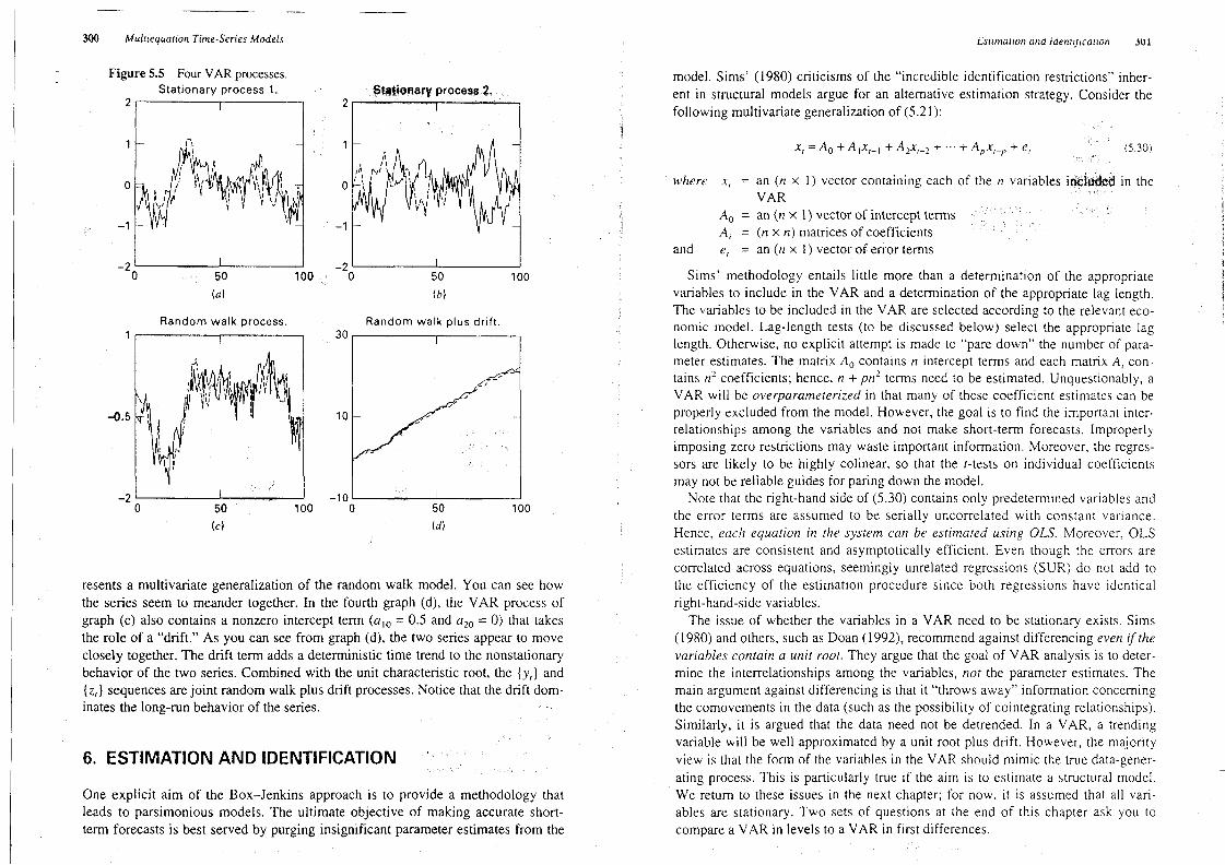
:MKj Muttieguation Time-seres Models

Figure S.S Four VAR processes.Stationary process 1.

Random walk process.

(c)

Ra n d o m wa lk p Iu s d ri ft .

30

#'

10 -

-100 50 1OO

(d)

S,t4#4:4#y procqo ;,2 E

1,1

. p. 1l .w

/ j1

. j? $ j,zO ! u' / l

l l 'v/

h l#t

-1

-20 50 100

(b1

resents a multivariate generalization of the random walk model. You can see howthe series seem to meander together. In the fourth graph (d), the VAR process ofgraph (c) also contains a nonzero intercept tenn (Jjc = 0.5 and azv = 0) that takesthe role of a

tdrift.'' As you can see from graph (d). the two series appear to moveclosely together. The drift term adds a detenninistic time trend to the nonstationary

behavior of the two series. Combined with the unit charactelistic root, the (y,)and(c,) sequences are joint random walk plus dlift processes. Notice that the drift dom-inates the long-run behavior of the series.

6. ESTIMATION AND IDENTIFICATION

One explicit aim of the ljox-lenkins approach is to provide a methodology thatleads to parsimonious models. The ultimate objective of making accurate short-term forccasts is best served by purging insigniticant parameter estimates from the

lf.llmallfpn tz?ld tdenlltcoton

model. Sims' (1980) criticisms of the ''incredible identification restrictions'' inher-ent in structural models argue for an alternative estimation strategy. Consider thefollowing multivaliate generalization of (5.21):

. k.,.,.

. .g,,. .

. . y. .''

k'

. . ..' 2..

x: = Atl + A 1..v,-1 + zta-vr-c + ... + Apxi-o + e:.E

2*;'

'(.q.'

' '

p'

.!llE' '

..

tsjj'i

.j.ijj= ZR (X X 1) VCCtOF COl1(Zi R illg CZO h Of the rl Valiables ilkizvzv in the

.:y 1.'

. 'y.:'.'.t

.';(. k.. .

VAR E

.. '. :...1 .k.. i . ').;

... L. 'l.y.).

.. .. ' . .! .E.'.y:,.'j.( ,.. .) .q .).Ao = an (n x l ) vector of intercept tenns q

.. ((..).. .

J 1 .r . . .. .zztf = n x n4 matlices of coefficients '

', = an (n x 1) vector of error tenns

Sims' methodology entails little more than a determination of the appropriatevariables to include in the VAR and a determination of the appropriate iag length,The variables to be included in the VAR are selected according to the relevant eco-nomic model. Lag-length tests (to be discussed below) select the appropriate 1aglength. Otherwise. no explicit attempt is made to

''pare

down'' the number of para-meter estimates. The matrix Ao contains n intercept terms and each matlix Af con-tains n2 coefficients; hence. n + pn2 tenns need to be estimated. Unquestionably, aVAR will be overparametered in that many of these coefficient estimates can beproperly excluded from the model. However. the goal is to find the important inter-relationships among the variables and not make short-tcrm forecasts. lmproperlyimposing zero restlictions may waste important information. Moreover, the regres-

sors are likely to be highly colinear. so that the J-tests on individual coefcients

may not be reliable guides for paring down the model.Note that the right-hand side of (5.30)contains only predetermined variables and

the error terms are assumed to be serially uncorrelated with constant variance.

Hence. each equation in the sysem can be estimated using OLS. Moreover, OLSestimates are consistent and asymptotically efficient. Even though the errors arecorrelated across equations, seemingly unrelated regressions (SUR) do not add tothe efficiency of the estimation procedure since both regressions have identicalright-hand-side variables.

The issue of whether the variables in a VAR need to be stationary exists. Sims( 1980) and others, such as Doan (1992),recommend against differencing even thevariables contain a unit root. They argue that the goal of VAR analysis is to deter-mine the interrelationships among the variables. not the parameter estimates. Themain argument against differencing is that it t'throws away'' information concemingthe comovements in the data (suchas the possibility of cointegrating relationships).Similarly. it is argued that the data need not be detrended. ln a VAR, a trending

valiable will be well approximated by a unit root plus dhft. However, the majority

view is that the form of the variables in the VAR should mimic the true data-gener-ating process. This is particularly true if the aim is to estimate a structural model.We return to these issues in the next chapter', for now. it is assumed that aII vari-

ables are stationary. Two sets of questions at the end of this chapter ask you tocompare a VAR in levels to a VAR in first differences.

302 Multiequation llme-kye/'fe,vModels

IdenlificalionTo illustrate the identiscation procedure, retum to the structural twcsvariable/first-order VAR represented by (5.19)and (5.20).Due to the feedback inherent in thesystem, these equations cannot be estimated directly. The reason is that zt is corre-lated with the error term eyt and y, with the error tenn Ea?. Standard estimation tech-niques require that the regressors be uncorrelated with the en'or term. Note there isno such problem in estimating the VAR system in standard form gi.e.,in the formof (5.22a)and (5.22b)).OLS can provide estimates of the two elements of Ao andfour elements of Al. Moreover, by obtaining the residuals from the two regressions.it is possible to calculate estimates of the variance of eLt, ez,, and of the covariancebetween el, and ecr. The issue is whether it is possible to recover a11the informationpresent in the plimitive system from the estimatcd system (5.19) and (5.20). Inother words, is the primative form identifiable given the OLS estimates of the VARmodel in the fonn of (5.22a)and (5.22b)?

ne answer to this question is tNo. unless we are willing to appropriately restrictthe primitive system.'' ne reason is clear if we compare the number of parametersin the stnlctural VAR with the number of parameters recovered from the standardfonn VAR model. Estimating (5.22a)and (5.22b)yields six coefficient estimates(t7lo,aw t7l j, al2, c21, and az and the calculated values of var(dl,), vart'ctl, andcovtelr, ec,). However, the primitive system (5.19) and (5.20)contains 10 parame-ters. In addition to the two intercept coefficients 'l() and bzz,the four autoregressivecfticients e/1

1. ylz,y21.and ycc,and the two feedback coefticients bLg and lay. thereare the two standard deviations cy and %. In all, the primitive system contains 10parameters, whereas the VAR estimation yields only nine parameters. Unless one iswilling to restrict one of the parameters, it is not possible to identify the primitivesystem',Equations (5.19)and (5.20)are underidentified. lf exactly one parameter ofte primitive system is restricted. the system is exactly identified, and if more thanone parameter is restricted, the system is overidentified.

One way to identify the model is to use the type of reeursive system proposedby Sims (1980).Suppose that you are willing to impose a restriction on the primi-tive system such that the coefficient !7clequals zero. Writing (5.19)and (5.20)withthe constraint imposed yields

.. ; .

Esktmaton and ldentthcatton 363

Xbw,premultiplicationof the primitive system by B ' yields: .

r.. . .. . . .

..

.

.

yt l -b12 l: l -':2-/

l l''/

12 A,,-1 t -7!

2 yr

= + + '

zt 0 1 bzv 0 l ''/

z)'y'cz

zt-1 0 l E.:,

or

hlo- :12/.720 '1

1- :12-21yt = +

z &col

Estimating the system using OLS yields the theoretical parameter estimates:

! j : : . yt = g j (; + (; j j yy..j + L; j zgj..j + '

j (

. . . zx.j.

u.j.

g tj p. cLt 6120 2 1Y/-1 22 t- 1 2J

whre a 3o= ll0 - bLzbzv

(71l = '11

- ?'l2't?cI

t712 ='12

- /7,2-/22

tzzo= b1v

tzcl='21

azz= cc

Var(t?!) = (52 + /72(5.2.; ! 2 z

vartca) = cuCovtpl, t?z) =

-?1zc2

2

(5,34a)(5.34b)

(5.34c)

yt= :lo - btzzt+ -/.

1.Y/-1+'l22r-l + es

zt= bzo+ .21.:,-1 + :222,.-1+ er/

Given the restriction (which might be suggested by a particular economicmodel), it is clear that zt has a contemporaneous effect on y,, but y, affects the (z,)'

- jsequence with a one-period lag. Imposing the restriction b23 = 0 means that B isgiyen by:

s-t = (,1-@5

2jl

Thus, we have nine parameter estimates a 1o, a j p , a 1a, azo, tzc j , azz, vart: ,),

vartpz), and covlcl ,

'c) that can be substituted into the nine equations above in or-der to simultaneously solve for b yo, b l c,

'?i

l ,

'/l

c, bco, '?c

l ,

''fzzs G2y,and c2z.Note also that the estimates of the (6v,1 and (6c, ) Sequences can be recovered.

The residuals from the second equation (i.e., the (::!,) sequence) are estimates of

the l 6c, ) sequence. Combining these estimates along with the solution for b l a al-

lows us to calculate the estimates of the (e ?Jsequence using the relationship t?l, =

yev,

- b 1c6c,.

Take a minute to examine the restriction. In (5.32).the assumption bz3 = 0 means

that y: does not have a contemporaneous effect on z:. ln (5.33), the restriction mani-

fests itself such that both 6 , and 6.cr shocks affect the contemporaneous value of y,,

but only 6,, shocks affect the contemporaneous value of zt. The observed values of

ez, are completely attfibuted to pure shocks to the (c?) sequence. Decomposing the

residuals in this triangular fashion is called a Choleski decomposition.

Q

Examples of Overidentified Systems

The interesting feature of overidentifying restrictions is that they can be tested.Suppose you wanted to further restrict (5.33)such that yc: = 0. Such a restriction

can have important economic implications; if ,21 = 0 and 'y2l= 0, contemporaneous

ey,shocks and lagged values of y/-j have no effect on z:. Hence. the null hypothesis#cl =

'yzl= 0 is equivalent to the hypothesis that (z/) is exogenous in that the (z,)

sequence evolves independently of (y,). Given the form of (5.33),the test that y2l =

0 is the test that tz21 in the VAR model is zero. To perform this test. simply estimate(5.33) and use a stest to test whether 4721 = 0.

Not all testable restrictions are this straightforward. Consider another version of(5.19) and (5.20)such that yyz= 'zl = 0:

software packages can test such nonlinear restzictions using the methodology dis-

cussed in Section 8.

7. THE IMPULSE RESPONSE FUNCTION

Just as an autoregression has a moving average representation, a vector autoregres-

sion can be written as a vector moving average (VMA). ln fact, Equation (5.27)isthe VMA representation of (5.21)in that the variables (i.e.,y, and z:4are expressed

in terms of the current and past values of the two types of shocks (i.e., dl, and 6c,).

The VMA representation is an essential feature of Sims' (1980) methodology in

that it allows you to trace out the time path of the various shocks on the variables

contained in the VAR system. For illustrative purposes. continue to use the two-

variable/tirst-order model analyzed in the previous two sections. Writing (5.22a)and (5.22b)in matrix fonn, we get

' = 'lo + '1 ,'/-1 + bl2c?+ 6yf1.

zt= bz, + bcly? + Y22z?-l+ ez,

To write tlw system in standard VAR fonn, we can use direct substitution'.j(,'j= j'u ,1o,j+ jua

(lj

u

,12,jj(;.-

tj+ j,E',i',jy' = &lo+ yI,y/-! + blzt&zo+ :2ly? + Y22z?-I + 6z?) + Eyf

z:= bzb+ l'zlt'lo + 'l 1y,-1 + btzzt + ex/) +'/zztt-.

+ e,,

It follows that

yt = J lo + a l 1.Y/-1+ t2 I 2C,-l + e 1/

zt = J2o + J2IA'?-I + &22C,-l + ez: .jy---'j- gv,.q+--.,

j,)--,-,-,--,)j'g--)-,----j

where tz,o = (:,0 + b,zbzzjl 1 - d7I2)zl)

a1 l--

I I/(l - b l 2b2 I )a ,2 = :12-722/(1- b 1:/21)

J20 = bzz + 1,2,1'1()24/(11- &lz@72l)

&2,= d72,-/1'l 1 - :12:2.)a,z=

'a2/(1- 7lcb2l)

Since et: = (ex,+ E7IcEu,)/(1 - lllzhcl) and ezt = (dujex,+ ez/)/(1 - hlcdhj). it followsthat

7 Equation (5.36) expresses yl and z, in terms of the (cIt) and (ea,) sequences.

However, it is insightful to rewrite (5.36)in terms of the (e.v,) and (6c/Jsequences.

From (5.23)and (5.24),tbe vector of errors can be written as

-.lj: E.vt

1 6 zl

so that (5.36)and (5.37)can be combined to fonn

Var(eI,) = (c2+ :2zc2)/(1 - Jpjzlzjlz'( . zVaz.tezfl = (cu + :21cy)/(l - 'lzlzl)

COv(dl?, eztt = tclO'y + bjzo'ztls - '12721) ''

'' '' t

g'c-,j- g#,,-j+k1/(1- -lc-cl ))y,..-,-jut'zi:tztlzaj'g-),,

-:112

jqEt.)'--

jOLS provides estimates of the six values of the aq and var(:1,), vartcz,), and

covtclr, cc,). These nine estimated values can be used with any eight of the nine

equations above to solve for hlo, bzo, 'lz. :21, 'j

1,'za.

cx, and %. Since there is an

extra equation, the system is overidentified. Unfortunately, the overidentifying re-striction here leads to nonlinear restlictions on the various aq. Nevertheless, many

Since the notation is getting unwieldy, we can simplify by defining the 2 x 2 ma-trix (j/ with elements k..

,lzu.))t)-,z,'-jizj

t..- (xt/ti-

306 Multiequation rn:-skrl'c. Models

Hcnce, the moving average representatin of (5.36)and (5.37)can be written intenns of the (6y,) and (ec,)sequences: '

yt #-

911(f) l2(f) es-j= + Xzt i' i-z 921(i) 22() 6c,-I..

'. . . . . . .

(. 'i.

''

tlyj

. ' . . E.. . . .; . . . . ) .:7.. # , / ''. . .. (' . .6 '.

'

.. .:.'

'. .) ... 4 j .: . y'. k.,i' (

y'

oo

t . . . . .: .. ). .: .. ..

. (..'

.. .. $ ..F ;. .

: E 5 ) ; j: ( :j:

z zz j. 4. jyo.yl: ) ( .

. '.' / .' : . .: ' ' ' ' ' ' ' '. '

i ca ()

average representation is an especially useful tool to examine the in-teraction betwecn the (y,)and (c,)sequences. The coefficients of 4)/can be used togenerate the effects of ey, and 6c, shocks on the entire time paths of the (y,) and (zt)sequences. If you understand the notatin, it should be clear that the four elementss(0) are impact multipliers. For example, the coefficient )z(0) is the instanta-neous impact of a one-unit change in ez, on yt. ln the same

qway, the elements j1(1)

and ():r.(1) are the one period responses of unit changes in es-l and Ew-j on yt, re-spectively. Updating by one pefiod indicates that $1j(1) and j/1) also representthe effects of unit changes in ex, and ecton yt.l.The accumulated effects of unit impulses in ey, and/or Ez, can be obtained by theappropriate summation of the coefficient.s of the impulse response functions. Forexample, note that after n periods, the effect of ,.t on the value f yt..n is (lc(n).Thus, after n periods, the cumulated sum of the effects of 6cf on the (y?)sequence is

The moving

/ ttt? 1??IPltt't;r .T$t'pvl l (;' I ' u l t t. I f llt

pure ey, or 6c? shocks. However, this methodology is not available to the researclersince an estimated VAR is underidentified. As explained in the previous section,knowledge of the various av and variance/covariance matrix )2 is not sufficient toidentify the primitive system. Hence, the econometlician must impose an additionalrestriction on the two-variable VAR system in order to identify the impulse re-SPOIASCS.

One possible identiscation restriction is to use Choleski decomposition. For ex-ample, it is possible to constrain the system such that the contemporaneous value ofy, does not have a contemporaneous effect on z:. Formally, this restriction is repre-sented by setting bzL = 0 in the primitive system. ln terms of (5.37),the error termscan be decomposed as follows:

= b'

e kr e7.?-

126c,

elt ez,

Thus, if we use (5.40), a11 the observed errors from the (e1: ) sequence are attrib-uted to z( shocks. Given the calculated (Ec,Jsequence, knowledge of the values ofthe (:j,) sequence and the correlation coefficient between eL: and cc,, allows for thecalculation of the (ey,)sequence using (5.39).Althoughthis Cholesk.i decomposi-tion constrains the system such that an Ey, shock has no direct effect c,, there is anindirect effect in that lagged values of y, affect the contemporaneous value of c,.The key point is that the decomposition forces a potentially important asymmetryon the system since an %t shock has contemmraneous effects on both y: and z:. Forthis reason (5.39)and (5.40)are said to imply an ordering of the vgriables. An

z:shock directly affects e1, and ezt but on 6x, shock does not affect c2?. Hence, cr ist rj() r,, ttl gy1) f.

Suppose that estimates of equations (5.22a)and (5.22b)yield the values ttlll = azv= 0, t7I l

= az; = 0.7, and c12 = t7cl = 0.2. You will recall that this is precisely thel used in the simulation reported in graph (a) of Figure 5.5. Also suppose thatmo e

the elements of the Z matrix are such that c2, = c2zand covtp j,, ez:) is such that thecorrelation,coefcient between t?l, and ez: (denotedby plc) is 0.8. Hence, the de-composed errors can be represented by8

.51.:E'

e 1t= 6y,; + 0.8EcI

(5.4 I)

; gz r= 6. t (j

.42

)C

The top half of Figure 5.6, parts (a) and (b), traces out the effects of one-unitshocks to Ec, and 6),, on the time paths of the (y?) and (zt) sequences. As shown in

;.ik the upper left-hand graph (a). a onc unit-shock in 6.a, causes z: to jump by one unit

,,, and y, to jump by 0.8 units. glRrom (5.41), 80% of the ec, shock has a contemporane-

!r. ous effect on e 1,.1 ln the next period, ecr..j returns to zero, but the autoregressive na-ture of the system is such that ytrb and z,+j do not immediately return tb their long-

qrnln values. Since z/+1= 0.2yr + 0.7c, + 6z,..l , it follows that c,.1 = 0.86 g0.2(0.8)+. 0.7(1) = 0.861.Similarly, y,+1= 0.7y, + 0.2c, = 0.76. As you can see from the figure,

n

9!2(i')aa()

.. . '.. (

''

. r

. ' ... .

..E.) .. ). . g:.'.

: ..

Letting n approach intinity yields the long-rtln multiplier. Since the (y,) and(ttl sequences are as'sumed to be stationary. it mut be the case that ibr a11j and kb

eo r.. j.y .t .2 ) is finit.''

' '' Fbk(i=o

The four sets of coefficients 4)t!(). (lc(/), z() and (zzi) are called the impulsere-sponse functfons. Plotting the impulse response functions (i.e.,plotting the coef-ficients of kl against ) is a practical way to visually represent the behavior of the(y,l and (z,)series in response to the various shocks. In principle, it might be pos-sible to know all the parameters of the primitive system (5.19)and (5.20).Withsuch knowledge. it would be possible to trace out the time paths of tle effects of

Figure 5.6

Mod e I 2 :

Fle$*. F.@to :zf s hoc k .1

.E. q . t

Ei

J' ' .'

(. 7 '' ( r .' '' E

Q.25

.**.50 1O 20

(c)

Solid line = fy;)sequence. Cross-hatch = (.:f)seq uence.note: ln a11cases e j ?

= 0.8vt + &yra nd ezt = ezr

the subsequent values of the (y/)and (c?) sequences converge to their long-run lev-els. This convergence is assured by the stability of thq system; as found earlier, thetwo characteristic roots are 0.5 and 0.9.The effects of a one-unit shock in Ew are shown in the upper-light-hand graph (b)of the t'igure.'rhe

asymme'y of the dezomposition is immediately seen by compar-ing the two upper graphs. A one-unit shock in ey, causes the value of y, to increaseby one unit; however, there is no contemporaneous c/-/cf on the value of z:, so thatyt = 1 and zt = 0. In the subsequent period, ey,+I returns to zero. The autoregressivenature of the system is such that y/+1 = 0.7y? + 0.2c/ = 0.7 and z,..t = 0.2yf + 0.7z, =

.0.2. T'he remaining points in the figure aze the impulse responses for periods y/..z

i /lt, iltputse ?s'cqptpl?.c i. l.tacl/fl/:i

. q' through yt.zo. Since the system is stationary, the impulse responses ultimately de-fCay.

Can you figure out the consequences of reversing the Choleski decomposition insuch a way that :12, rather than l?cj, is constrained to equal zero? Since matrix .4

1 issymmetrical (i.e., a , ,

= tzaa and a , 7 = a,z , ), the impulse responses of an 6.,., shockwould be similar to those in graph (a) and the imptllse responses of an Ec, would be

( similar to those in graph (b).The only difference would be that the solid line repre-i.. .1 sents the time path of the (zf)sequence and the hatched line the time path of the

tF?l Seqtlence.

As a practical matter, how does the researcher decide which of the alternative de-compoqitions is most appropriate? ln some instances, there might be a theoretical

reason to suppose that one valiable has no contemporaneous effect on the other. lnthe terrorism/tourism example, knowledge that terrorist incidents affect tourism

. .i yy

with a lag suggests that terrorism does not have a contemporaneous effect ontourism. Usually, there is no such a pfiori knowledge. Moreover, the very idea of

,imposing a structure on a VAR system seems contrary to the spirit of Sims' argu-ment against t'incredible identifying restrictions.'' Unfortunately, there is no simple

way to circumvent the problem; identification necessitates imposing some stnlcture

on the system. The Choleski decomposition provides a minimal set of assumptionsthat can be used to identify the plimitive mode1.9

lt is crucial to note that the ilnportance ofthe ordering depends on the magnitude

of the correlation coemcient l/clw'tr?t e)( and or Let this correlation coefficient be. .. j.:.j

denoted by p :2 so that p jz = cjc/clcc. Now suppose that the estimated model yields

a value of 12such that pj2 is found to be equal to zero. ln this circumstance, the or-dering is immatelial. Fonnally, (5.41)and (5.42)become l,

= 6.yt and ez, = 6a, whenpI2 clz 0. Thus, if there is no correlation across equations, the residuals from the y?and zt equations are necessarily equivalent to the 6y, and ezt shocks, respectively. Atthe other extreme, if pIc is found to be unity, therc is a single shock in the systemthat contemporarily affects both variables. Under the assumption /zl = 0, (5.41)and(5 . 4 2 ) b e co me e : ,

= E z : a n d e 2 := e z , ; in s t e ad , u nde r t he a ssu m p t i o n

l7lc= 0, (5.41)apd (5.42)become cj, = 6x, and ezt = es. Usually, the researcher will

want to test the significance.of

plc; as a rule of thtlmb. if lplc I > 0.2. the correla-'' tion is deemed to be significant. lf 1pjz I > 0.2, the usual procedure is to obtain the

i! impulse response function using a particular ordering. Compare the results to the

impulse response function obtained by reversing the ordering. If the implications

are quite different, additional investigation into the relationships between the vari-

ables is necessary.The lower half of Figure 5.6, parts (c) and (d), presents the itnpulse response

functions for a second model; the sole difference between models 1 and 2 is the

change in the values of 4712 and tzzj to-0.2.

Model 2 was used in the simulation re-

t ported in graph (b)of Figure 5.5. The negative off-diagonal elements of A $ weaken

the tendency for the two series to move together. Using the impulse responses rep-i resented by (5.4l ) and (5.42)(d) shows that. y,.1 = 0.7y, - 0.2c, = 0.7 and z,.! =

l 'F'1

I.

-0.2y,

+ 0.7z,+I =-0.2.

Tracing out the entire time path yields the lower-right-handl

...E

- .).)@:;(1. ...... ..,L.?(..'. .

'.

.. .'. ' '.

E.t .:..t.-.#..E'. . .,:. . - . .

. .' .:..' k ..;'. 'ty.;''.'(

t'i

(' ' . '

jj

310 Multiequation Time-series Models

graph (d) of the figure. Since the system is stable, both sequences eventually con-- verge to zero.The lower-left-hand graph (c) traces out the effect of a one-unit 6c, shock. In pe-' E riod 1, zt rises by one unit and y, by 0.8 units. ln period t + 1), er,+I returns to zero,

, but the value of )qw is 0.7y, - 0.2c, = 0.36 and the value of r,+j is-0.2y,

+ 0.7z, =

0.54. The points represented by l = 2 through 20 show that the impulse responses.

, Et converge to zero.

.L . . . .

; Variance Decomposition . . . .

Since unrestricted VARS are overparameterized, they are not pmicularly useful forshort-term forecasts. However, understanding the properties of the forecast errors isexceedingly helpful in uncovering interrelationships among the variables in the sys-tem. Suppose that we knew the coeftkients of Ao and A j and wanted to forecast thevarious values of xt.vt.conditional on the obselwed value of xt. Updating (5.21)oneperiod (i.e.,x,+l = Ao + zt 1.z., + c,+j) and taking the conditional expectation of .z',+l

, weobtain

Tlte lmpulse Response Function 311

the forecst errors in terms of the (6.,)sequence. If we use (5.38) to conditionallyforecast .r,+j

, the one-step ahead forecast en'or is 06,+1 . In general,

xt..n= p.+ fel+a-

i=0

t theriuytiod feast irror.x

wn- Etxt..nisS0

' '. ( . ' '

Note that the one-step ahead forecast error is 1,+1 -

'z/+j

= tuj . similarly,updat-t jn two periods we get# ,

xtn = Xo + X 1.1,+1 + etwz= tl + A l(A()+ Ajx, + c,+j) + et..z.1

('

tf tak conditional expectations the two-step ahead forecast of x isWe, ;+a

E'

..'.'.... .'...

; .. . . . t. j:'.;.) .. .. .

....

: s x = l + A,)x, + Alx.r )

. ( 1. 1'.1.. :7! I /'

The two-step ahead forecast en'or (i.e., the difference between the realization ofxt..zand the forccast) is e,+2 + AjG+l. More generally, it is easily verified that then-step ahead forecast is

Denote the variance of the n-step ahead forecast error variance of y,+nas cy(n)2

Since al1 values of (jkl are necessarily nonnegative, the variance of the forecasten'or increases as the forecast horizon n increases. Note that it is possible to decom-

pose the n-step ahead forecast error variance due to each one of the shocks.Respectively, the proportions of cy(n)2 due to shocks in thc (6y,) and (ezt)se-quences are

The forecast error variance decomposition tells us the proponion of the move-ments in a sequence due to its ''own'' shocks versus shocks to the other variable. X'Ek, shocks explain none of the forecasterror variance of (yt) at all forecasthori-

zons, wc can say that the (y:)sequence is exogenous. ln such a circumstance, the

(y,) sequence would evolve independently of the 6r, shocks and (c,) sequence. Atthe other extreme, <zt shocks could explain al1 the forecast error variance in the (y,)sequence at al1 forecast horizons, so that (y,) would be entirely endogenous. ln ap-plied research, it is typical for a variable to explain almost a11its forecast error vari-

,,2 (j)2 + j (j)2+ - . . + 4 Ln- j)2 ).EE

. () O-c(Y12 ( l c j 2and.k: t 2

c y (n)

and the associated forecast error is

e + A ld,+u-) + A2ld,+a-z+ .-. + A2-tet+j14-#!

We can also consider these forecast errors in terms of (5.38)(i.e.,the VMA formof the model). Of course. the VMA and VAR models contain exactly the sape in-fonnation, but it is convenient (and a good exercise) to describe the properties of

312 Multiequaion Time-kries Models

ance at short horizons and smaller proportions at Ionger horizons. We would expectthis pattern if ec, shocks had little contemporaneous effect on y,, but acted to affectthe (y,)sequence with a lag.

Note that the variance decomposition contains the same problem inherent in im-pulse response function analysis. ln order to identify the (ey,)and (6z,) sequences,it is necessary to restrict the B matrix. The Choleski decompostion used in (5.39)and (5.40)necessiutes that all the one-period forecast error variance of zt is due toez,.If we use the alternative ordeling, all the one-period forecast error vafiance of ytwould be due to eyt. The dramatic effects of these altemative assumptions are re-duced at longer forecasting horizons. ln practice. it is useful to examine the vari-

ance decomposition at various forecast horizons. As n increases, the variance de-compsitions should converge. Moreover. if the correlation coefficient p Ic issignificantly different from zero, it is customary to obtain the valiance decomposi-tions under valious orderings.

Nevertheless, impulse response analysis and variance decompositions (togethercalled innovation accounting) can be useful tools to examine the relationships

among economic variables. If the correlations among the various innovations aresmall, the identification problem is not likely to be especially important. The alter-native orderings should yield similar impulse responses and variance decomposi-tions. Of course, the contemporaneous movements of many economic variables arehighly correlated. Sections 10 through 13 consider two attractive methods that canbe used to identify th structural innovations. Before examining these techniques,we conjider hypothesis testing in a VAR framework and reexamine the interrela-tionships between terrorism and tourism.

8. HYPOTHESIS TESTING

In principle, there is nothing to prevent you from incorporating a large number ofvmiables in the VAR. It is possible to construct an n-equation VAR with eachequation containing p lags of a1l n variables in the system. You will want to includethose variables that have important economic effects on each other. As a practicalmatter, degrees of freedom are quickly eroded as more variables are included. Forexample, with monthly data with 12 lags, the inclusion of one additional valiable

uses an additional 12 degrees of freedom. A careful examination of the relevant

theoretical model will help you to select the set of variables to include in your VARmodel.

An n-equation VAR can be represented by

.. .. .. !. '.. .,(' '. '

..'!.

.' .':.'). .ly'..

where o= the parameters representing intercept terms

Aijl = the polynomials in the Iag operator L.

The individual coefficients of Aql are denoted by Jf/1), /f/2),. . Since all

equations have the same 1ag length. all the polynomials Atjlu) are of the same de-

gree. The tenns eo are white-noise disturbances that may be correlated. Again. des-

ignate the variance/covariance matrix by , where the dimension of 12iS (n x n).

In addition to the detenuination of the set of vafiables to include in the VAR, it

is important to determine the appropriate lag length. One possible procedure is to

allow for different 1ag lengths for each variable in each equation. However. in or-

der to preselwe the symmetry of the system (andto be able to use OLS efficiently),

it is common to use the same 1ag length for all equations. As indicated in Section

6, as long as there are identical regressors in each equation, OLS estimates are

consistent and asymptotically efticient. If some of the VAR equations have regres-

sors not included in the others, seemingly unrelated regressions (SUR) provide ef-

ficient estimates of the VAR coefcients. Hence, when there is a good reason to

1et 1ag lengths differ across equations, estimate the so-called near VAR using

SUR.ln a VAR. long lag lengths quickly consume degrees

p, each of the n equations contains np coefficients plus the intercept term.

Appropriate lag-length selection can be critical. lf p is too small, the model is mis-

specified',if p is too large. degrees of freedom are wasted. To check lag length, be-

gin with the longest plausible length or longest feasible length given degrees-of-

freedom considerations. Estimate the VAR and form the varianee/covariance

matrix of the residuals. Using quarterly data, you might start with a lag length of 12

quarters based on thc a prioti notion that 3 years is sufticiently long to capture the

system's dynamics. Call the vadance/covariance matrix of the residuals from the

12-1agmodel Elz. Now suppose you want to detennine whether eight lags are ap-

propliate. After all, restrkting the model from 12 to eight lags would reduce the

number of estimated parameters by 4n in each equation.

Since the goal is to determine whether lag 8 is appropriate for a11equations, an

equation by equation F-test on lags 9 through 12 is not appropliate. lnstead, the

proper test for this cross-equation restriction is a likelihood ratio test. Reestimate

the VAR over the same sample period using eight lags and obtain the variance/co-

vadance matrix of the residuals 1k. Note that Ek pertains to a system of n equations

with 4n restrictions in each equation for a total of 4n2 restrictions. The likelihood

ratio statistic is

of freedom. lf lag length is

(otloglr. l - log lslal)

' However, given the sample sizes usually found in economic analysis, Sims

(1980) reeommends usingA'1, Alc z4l 1(-) AI2(-) Aln(f-) .:1/-1

e'l,

xzt A2o Acl(f-) Ac2(L) AnLj .n,-1

ezt= + +

xn: Aao Aa1(L) Anzl-v) Auu(,) A'n-j ent

314 Multiequation Time-series Models. .' ' ' . ''

where = number of usable observations

= number of parameters estimated in each equation of the unre-stricted system

log IIk I = is tlle natufal logarithm of the deterrninant of Ik.

In the example at hand, c = 12n + 1 since each equation of the unrestricted modelhas 12 lags for each variable term plus an intercept.

nis statistic has the asymptotic z2distribution with degrees of freedom equal tote number of restrictions in the system. ln the example under consideration, thereare 4n restrictions in each equation, for a total of 4n2 restrictions in the system.Clearly, if the restriction of a reduced number of lags is not binding, we would ex-

ct log 1Es l to be equal to log I12laI. Large values of this sample statistic indieatethat only eight lags is a binding restriction; hence, a rejection of the null hypothesisthat lag length = 8. lf the calculated value of the statistic is less than :2 at a prespec-ified significance level. we would not be able to reject the null of only eight lags.At that point, we could seek to determine whether four lags were appropriate byconstructing

(z- clllog lz.l - Iog lr. I)Considerable care should be taken in paring down lag length in tbks fashion.

Often, this procedure will not reject the null hymtheses of eight versus 12 lags andfour versus 8 lags, although it will reject a null of four versus 12 lags. The problemwith paling down thc model is that you may lose a small amount of explanatorypower at each suge. Overil, the total loss in explanatory power can be signitkant.In such circumstances, it is best to use the longer 1ag lengths.

nis type of likelihood ratio test is applicable to any type of cross-equation re-tri tion Let X and Z be the variance/covariance matrices of the unrestriced andS C .

u r

restricted systems, respectively. lf the equations of the unrestdcted model containdifferent regressors. let c denote the maximum number of regressors contained inthe longest equation. Asymptotically, the test sutistic:

(T- clgog (z+( - log (z.1)

has a zl distribution wit degrees of freedom equal to the number of restrictions inthe system.

To take another example, suppose you wanted to capture seasonal effects by in-cluding three seasonal dummies in e'ach of the n equations of a VAR. Estimate theunrestricted model by including the dummy variables and estimate the restrictedmodel by excluding the dummies. ne total number of restrictions in te system is3n. If lag length is p, the equations

.of

the unrestricted model have np + 4 parame-ters (np lagged variables, the intercept, and the three seasonals). For F usable obser-vations, set c = np + 4 and calculate the value of (5.45).lf for some prespecifiedsignitkance level, this calculated value k2 (with3/1 degrees of fyeedom) exceeds

Hypohesis Testing

the critical value, the restriction of no seasonal effects can be rejected. Equation(5.45) can also be used to test the type of nonlknear restliction mentioned in Section6. Estimate the restlicted and unrestricted systems. Then compare the alculatedvalue of (5.45)to the critical value found in a :2 table,

The Iikelihood rati/ test is based c)n asymptotic theory that may not be very use-fu1 in the small samples available to time-series cconometricians. Moreover, the

likelihood ratio test is only applicable when one model is a restricted version of the

other. Alternative test criteria to determine appropriate lag lengths and/or seasonal-

ity are the multivariate generalizations of the AIC and SBC:

'. .. . ..

'

. .

,'

. . .

'.'

.. ..' ...' ..

L','

., g . . . . .

r'

'. .. .. yi.

...;

y' .; :. !.:

. j. , T .(..7. L?. ...

, y ....

. . . ;

where = detenminant of the variance/covaliance matrix of the residuals

= total number of parameters estmated in aII equations.

Thus, if each equation in an n-variable VAR has p lags and an intercept, N = nlp +

n.,each of the n equations has np lagged regressors and an intercept.Adding additional regressors will reduce 1og lE l at the expense of increasing N.

As in the univaliate case, select the model having the lowest AIC or SBC value.

Make sure that you adequately compare the models by using the same sample pe-riod. Note that these statistics are not based on any distributional theory'. as suchthey are not used in esting the type of cross-equation restrictions discussed inSection 6.

z&!Id:Elr= :;r'''IL4::),li;I::i(:;l ..1..:2 k''h,'-

..

.... t .......

.,. ...' . .-

...

..... :

. .). .......

.....-..

tii;B'4:(((2= ir''-l :)i114l(lil:il ..1.. .?'h,/' ILali;(7;!-'724... ,. ..q.-. .?.....

,r)..?.-.)...- . . ). .. .

. :...... ..t''.#

. ...t.-

r.,.)'.); .

Granger CausalityA test of causality is whether the lags of one variable enter into the equation foranother variable. Recall that in (5.33),it was possible to test the hypotheses that

a13 = 0 using a J-tcst. In a two-equation model with p lags. (z,) does not Granger

cause lc,) if and only if a11the coefficients of Aajtf,l are equal to zero. Thus, if (y,)does not improve the forecasting performance of (c?),then (y,)does not Granger

cause tz,) . The direct way to determine Granger causality is to use a standard F-test

to test the restliction:

/c,(1)= /21(2) = u1(3)= ''' = 0

ln the n variable case in which A,y(L)represents the coefficients of lagged values

of variable j on variable f, variable j does not Granger cause variable i if all coeffi-

cients of the polynomial Ao.L) can be set equal to zero.Npte that Granger causality is a weaker condition than the condition fpr ygg.,lle-

ity. A necessary condition for the exogeneity of (c,) is for current and past values

'''f'ty

) to not affect lc,). To explain. reconsider the VMA model. ln our previousO r

example of the two-variable VMA model, (y,J does not Granger cause (z7 if and

316 Hultiequation Time-kries Models

only if all coefticients of (2l(f)= 0 for f > 0. To sketch the proof, suppose that allcoeftkients of Gl(f)are zero for i > 0. Hence, z,+1is given by

Co

z,+l= i-+ 2I (0)6 r+l + 22()6z,+j-j

y =0

If we forecast z,+l conditional on the value of z,, we obtain the forecast errorGl(0)Ex,+l + #22(0)ez,+j. Given the past value of z,, infonnation concerning past val-uesof y, does not aid in forecasting zt. In other words, for the VAR(1) model underconsideration, Ejzt..j 1z,) = f',(c,+j lc,,z.Thc only additional information contatned in yt are the past values of (6y,).However, such values do not affect zt and so cannot improve on the forecasting per-formance of the z, sequence. Thus, (y,)does not Granger cause (z;). However, if#zj(0) is not equal to zero, (z,) is not exogenous to (ytl. If G1(0)is not zero, pureshocks to yt..j (i.e.,6y,+l) affect the value of zf..leven though the (y,)sequence doesnot Granger cause the (,R) sequence.

A block exogeneity test is useful for detecting whether to incorporate a variableinto a VAR. Given the aforementioned distinction between causality and exogene-ity, this multivariate generalization of the Granger causality test should actually becalled a

t'block causality'' test. In any event. the issue is to determine whether lagsof one valiable-say, w,--Granger cause any other of 4hevariables in the system.ln the' threc-variablc case with w,. y,, and z:, the test is whether lags of w, Grangercause either y, or r,. In essence, the block exogenity restricts all lags of w, in the y,and z, equations to be equal to zero. This cross-equation restriction is properlytested using the likelihood ratio test given by (5.45).Estimate the yt and zt equa-tions.using p lagged values of (y,), (z,) , and (w,)and calculate E.. Reestimate thetwo equations excluding the lagged values of (w,Jand calculate Er. Next. t'indthelikelihood ratio statistic:

Example of t2 Simple VAR: Terrorism tlnd Fluriym fn Spain 317

wing groups, which included the Anti-Fascist Resistance Group of October l(GRAPO), the ETA, the now defunct International Revolutionary Armed Front

E. .(FRAP), and Iraultza. Most incidents are attributed to the ETA (Basque Fatherland

and Liberty) and its splinter groups. such as the Autonomous Anti-capitalist'

Commandos (CAA). Right-wing terrolist groups included the Anti--rerrorist Liber-ation Group (GAL), Anti-Tenorism ETA, and Warriors of Christ the King. Catalanindependence groups, such as Free Land tTerra Lliure) and Catalan Socialist Partyfor National Liberation, have been active in the late 1980: and often target U.S,businesses.

The transfer function model of Section 3 may not be appropriate because of feed-back between terrorism and tourism. lf high levels of tourism induce terrorist activ-ities, the basic assumption of the transfer function methodology is violated. ln fact,there is some evidence that the terrorist organizations in Spain target tourist hotelsin the summer season. Since increases in tourism may genrate terrorist acts, theVAR methodology allows us to examine the reactions of tourists to terrorism andthose of terrorists to tourism. We can gain some additional insights into the interre-lation between the two series by pedbrming causality tests of terrorism on tourismand of tourism on terrorism. Impulse response analysis can quantify and graphicallydepict the time path of the effecrs of a typical terrorist incident on tourism.

We assembled a time series of al1 publicly available transnational terrorists inci-dents that took place in Spain from 1970 through 1988. In total, there are 228months of observation in the time series; each observation is the number of terrolistincidents occurring that month. The tourism data are taken from various issues ofthe National Statistics Institute's (Estadistic lnstitute Nacional) quarterly reporls. Inparticular, we assembled a time series of the number of foreign tourists per monthin Spain fcr the 1970 to 1988 period.

Empirical Methodology

Our basic methodology involves estimating toulism and terrorism in a vector au-toregression (VAR) framework. Consider the following system of equations'.(r- cltlog lsr! - log Iz.1)

As in (5.45),this statistic has a :2 distribution with degrees of freedom equal tolp (sincep lagged values of (w,) are excluded from each equation). Here, c = 3,+ 1 since the two unrestricted y? and zt equations conuin p lags of (y,), lz,) . and(w,) plus a constant.

n, = a10 + A j!(,)n,-I + /! lc(f,-! + e 1,

it = a20 + Ac1(.)n,-l + XzztLlt-l + ezt

9. EXAMPLE OF A SIMPLE VAR: TERRORISM ANDTQURISM IN SPAIN

In Enders and Sandler (1991),we used the VAR methodology to estimate the im-pact of terrorism on toulism in Spain during the period from 1970 to l 98'8. Mosttransnationalterrorist incidents in Soain during this rutrnd were nwnvtrots.,.l hx, 10'.-

where n, = the number of toulists visiting Spain during time period t

,= the number of transnational terrorist incidents in Spain during t

ao = are the 1 x 13 vectors containing a constant, 11 seasonal (monthly)dummy variables, and a time trend

Aij = the polynomials in the lag operator Lei, = independent and identically distributed disturbance terms such that

Eebtezf) is not necessarily zero

Although Sims (1980) and Doan (1992) recommend against the use of a deter-mlnl ckio 11 mo ev-onzl Ax?o rloo clocl nfaf f fa lao#xrl tlasx r n/-I N?; c.o Wo ov rh/ar; m/antfxfj w th

several altemative ways to model the series; thc model including the time trend hadyielded the best diagnostic statistics. Other variants included differencing (5.46)and (5.47)and simply eliminating the trend and letting the random walk plus driftterms capture any nonstationary behavior. Questions5 and 6 at the end of thischapter ask you to compare these alternative ways of estimating a VAR.

The polynomials AlatLl and A2I(f) in (5.46)and (5.47)are of particular interest.lf all the coefficients of A21are zero, then knowledge of the tourism selies does notreduce the forecast error variancc of terrorist incidents. Formally, tourism would

'

not Granger cause terrorism. Unless there is a contemporaneous response of terror-ism to tourism, the terrorism series evolvcs independently of toulism. In the sameway, if a1l te coefficients of A!a.(fz)are zero, then tenorism does not Granger causetoulism. The absence of a statistically signitscant contemporaneous correlation ofthe error terms would then imply that terrorism cannot affect toulism. If. instead.any of the coeftkients in these polynomials differ from zero, there are interactionsbetween the two series. In case of negative coeftkients of Aja(L), terroism wouldhave a negative effect on the number of foreign tourist visits to Spain.

Each equation was estimated using 1ag lengths of 24, l2, 6, and 3 months (i.e.,for four estimations, we set L = 24, 12. 6, and 3). Because each equation has identi-cal right-hand-side variables, ordinary least squares (OL.S) is an efficient estimationtechnique. Using :2 tests, we determined that a lag length of 12 months was mostappropriate (reducingte lengt.h from 24 to 12 months had a :2 value that was sig-nificant at the 0.56 level, whereas reducing the lag Iength to 6 months had a :2value that was signitkant at the 0.049 level). ne A1C indicated that 12 lags wereappropriate, whereas the SBC suggested we could use only six lags. Since we wereusing montly data, we decided to use the 12 lags.

To ascertain the imporunce of the interactions between the two sees, we ob-tained the variance decompositions. ne moving average representations of Equa-tions (5.46)and (5.47)express nt and it as depcndent on the current and past valuesof both ld1,)and (cz,Jsequences:

torization had no qualitative effects on our results (thecontemporaneous correlationbetween cI, and ezt was

-0.0176).

. ..'.'.....

.'...

.'.......

.'......'..'.

'.

'

(

q'

'

. . .'.

'' ' '

'

.' q'' ' .

'

.'''.''

''Empirical ResultsWith a 24-month forecasting horizon used, the variance decompositions are re-ported in Table 5.3. in which the significance levels are in parentheses. As ex-pected. each time series explains the preponderance of its own past values', nt ex-plains over 91% of its forecast error valiance, whereas i: explains nearly 98% of itsforecast en'or valiance. It is interesting that terrorist incidents explain 8.7% of theforecast error varianc,e of Spain's tourism, whereas tourism explains only 2.2% ofthe forecast en-or variance of terrorist incidents. More important, Granger causalitytests indicate that the effects of terrolism on toulism are significant at the 0.006level, whereas the effects of toulism on terrorism are not significant at conventional

levels. Thus, causality is unidirectional: Terrorism affects toulism but not the re-

verse. We also note that the terrorism series appears to be autonomous in the sensethat neither series Granger causes it at conventional levels. This result is consistent

with the notion that terrorists randomize their incidents, so that any one incident isnot predictable on a month-to-month basis.

Forecasts from an unreseicted VAR are known to suffer from overparameteriza-tion. Given the results of the variance decompositions and Granger causality tests.we reestimated (5.46)and (5.47) restricting a11the coeftkients of AzltLl to zero.Because the right-hand variables were no longer identical, we reestimated the equa-tions with seemingly unrelated regressions (SUR). With the resulting coefficientsfrom the SUR estimates. the effects of a typical terrorist incident on Spain'stoufism can be depicted. In tenns of the restricted version of (5.49).we set a11 ejr-yand ezt-.yequal to zero for j > 0. We then simulated the time paths resulting fromthe effects of a one-unit shock to ezr. 'The time path is shown in Figure f

.7,

where

the vertical axis measures the monthly impact on the number of foreign tourists

and the horizontal axis the months following the shock. To smooth out the series,

Table 5.3

where co and ds are Nectors eonmining eonstants. the l l seasonal dummies, and atrend; and cv, cay,Jjy.,and dzj are parameters.

Because we cannot estimate (5.48)and (5.49)directly. we used the residuals of(5.46) and (5.47)and then decomposed the vafiances of nt and , into the percent-ages attlibutable to each type of innovation. We used the orthogonalized innova-tions obtained from a Choleski decomposition'. the order of the variables in the fac-

Variance Decomposition Percentage of 24-Month Error Variance ),i $

Typical shock inPercent of forecast' :.j '

y6.:

'

Ei.' .r j.E .

('

.(..

error variance in n, ;?

91.3

8.7

(3x E- 15) (0.006)2.2 97,8

(17.2) (93.9)

Note: T'he numbers in parentheses indicate the significance Ievel for thejoint hypothesis that a11lagged coefticients of the variable in ques-tion can be sct equal to zero.

32: Hultiequation Time-series Jfode/.

. . . . .(''. Figur 5.7

we present the time path of a 3-month moving average of the simulated tourism re-. (.q

k'

. .....E'

.

y'

.g

.'r'

.;,(..'..

.'sponse function.

' After aettypical'' tenorist incident tourism to Spain begins to decline in the third

E; month. After the sixth month. tourism begins to revert to its odginal level. Theredoes appear to be a rebound in months 8 and 9. There follows another drop intourism in month 9, reaching the mximum decline about 1 year after the originalincident. Obviously, some of this pattern is due to the seasonality in the series.However, tourism slowly recovers and generally remains below its preincidentlevel for a substantial period of time. Aggregating a1136 monthly impacl, we esti-mate that the combined effects of a typical transnational terrorist incident in Spainis to decrease the total number of foreign visits by 140,847 people. By compmison,

a total of 5,392.(* tourists visited Spain in 1988 alone.

Sructural V'AS.C

Even though the model is underidentified, an appropriately specified model willhave forecasts that are unbiased and have minimum variance. Of course, if we had

a priori information concerning any of the codficients, it would be possible to im-

prove the precision of the estimatcs and reduce the forecast-error vafiance. A re-searcher interested only in forecasting might want to tlim down the overparmeter-ized VAR model. Nonetheless, it should be clear that forecasting with a VAR is amultivariate extension of forecasting using a simple autoregression.

The VAR approach has been criticzed as being devoid of any economic content.The sole role of the economist is to suggest the appropriate variables to include inthe VAR. From that point on, the procedure is almost mechanical. Since there is solittle economic input in a VAR, it should not be surprising that there is little eco-nomic content in the results. Of course, innovation accounting does require an or-dering of the valiables, but the selection of the orderng is generally ad hoc.

Unless the underlying structural model can be identified from the reduced-form

VAR model. the innovations in a Cholcski decomposition do not have a direct eco-nomic interpretation. Reconsider the two-variable VAR of (5.19)and (5.20):

yt+ lcc? = l,0 +',

l.'.'f-l + 'l2c?-1 + %tbzlyr+ zt = bzo + -f21)',-1 + -/222,-.1 + %t

so that it is possible to write the model in the form of (5.22a)and (5.22b):

lb = t7 !0 + a l 1A',-1+ /1 2Cr- 1 + e l ,

zt = 52o + &2lA'r-l+ 5222,-1 + P2?

where the various aij are defined as in (5.21).For our purposes, the imponant pointto note is that the two en'or terms e 1, and ezt are actually colposites of the underly-ing shocks %tand 6z?. From (5.23)and (5.24),

Although these composite shocks are the one-step ahead forecast errors in )'t and

z?,they do not have a stnlctural interpretation. Hence, there is an imprtant differ-

ence between using VARS for forecasting and using them for economic analysis. In(5.50), ejt and e2, arc forecast errors. If we are interested only in forecasting, the

components of the forecast errors are unimportant. Given the economic mdel of(5.19) and (5.20),Ey, and Ec, are the autonomous changes in y, and z: in period t, re-spectively. If we want to obtain an impulse response function or a variance decom-position to trace out the effects of an innovation in yt or cr, it is necessary to use the

10. STRUCTURAL VARS

Sims' (1980)VAR approch has the desirabl property that al1 variables are treatedsymmetrically, so that the econometrician does not rely on any

t'incredible identifi-cation restrictions.'' A VAR can be quite helpful in examining the relationships

among a set of economic valiables. Moreover, the resulting estimates can be used

for forecasting purposes. Consider a first-order VAR system of the type representedby (5.21):

xt = Ac + A jauj + et

Although the VAR approach yields only estimated viues of An and Al, for e#ptyk.sition pufposes, it is useful to treat each as being known. As we saw in (5.43j4

iVE

322 Multiequation Tlme-series Models

structural shocks (i.e., Ex, and %t),not the forecast errors. The aim of a structuralVAR is to use economic theory (ratherthan the Choleski decomposition) to recoverthe structural innovations from te residuals ft'I,) and (r2,1.

The Choleski decomposition actually makes a strong assumption about theunderlying structural errors. Suppose, as in (5.32),we select an ordering such thatbzt = 0. With this assumption, te two pure innovations can be recovered as

Struclural 7A/IJ 31.3

Equation (5.2l ) is obtained by prenlultiplying by B- to obtain

6 r= c:, - bbzezt

y

Defning zztll = :-lro, zt 1 = #-'r,, and el = #-': yields the multivariate general-/

ization of (5.21). The problem, then. is to take the observed values of et and restrict

the system so as to recover 6,, as e, = Ben However. the selection of the valious bv

cannot be completely arbitral-y. The issue is to restrict the system so as to (1) re-cover the various (E,) and (2) preselwc the assumed error structure concerning the

independence of the various lef,) shocks. To solve this identification probiem. sim-ply count equations and unknowns. Using OLS. we can obtain the vafiance/covari-

ance matrix Z:

C ln

(52N

2C

whea>4,h2 tlzept o Z i! pnstructed as the sum:

.'

. . '.

)'

Forcing )21 = 0 is equivalent to assuming that an innovation in y, does not have acontemporaneous effect on zt. Unless there is a theoretical foundation for this as-sumption, the underlying shocks are improperly identified. As such, the mpulse re-

'jsponses and variance decompositions resulting from this improper identification ycan be quite misleading.

If the correlation coefticient between ekt and ez: is low, the ordering is not likely i

to be important. However, in a VAR with several variabless it is improbable that allcon-elationswill be small. After all. in selecting the variables to include in a model,you are likely to choose variables that exhibit strong comovements. When theresiduals of a VAR are correlated, it is not practical to tl'y all alteriative orderings.With a four-variable model, there are 24 (i.e.,4!) possible orderings.

Sims (19B6)and Bemanke (1986)propose modeling the innovations using eco-'nomic analysis. To understand the procedure, it is useful to examinc the relation-ship between the forecast errors and structural innovations in an n-valiable VAR.Since this relationship is invaliant to lag length, consider the first-order model with

n variables: E

I

:21

bnL

cc

zc . = (l/F)

-

e et) ? jlt = 1

ln AI (-. l el ?

zn..:72?-1

62J

+

nn -Lr-l qnt

or in compact fonn,

Since E is symmetric, it contains only (n2+ n)/2 distinct elements. There are n e1-

i ements along the principal diagonal, (n - 1) along the t'irstoff-diagonal, n - 2 alongthe next off-diagonal, . . .

, and one corner element for a total of (nl + a)/2 free ele-

ments.Given that the diagonal elements of B are a1l unity, B contains n2 - rl unknown

values. In addition, there are the n unknown values vartEf,) for a total of n2 un-known values in the structural model (i.e..the /2 - rt values of B plus the rl values

vartesll. Now, the answer to the identitkation problem is simple; in order to iden-tify the n2 unknowns from the known (n2+ n)/2 independent elements of E, it is

nccessary to impose an additional n2 - g(n2+ n)/2) = (n2 - n)/2 restrietions on the

system. This result generalizes to a model with p lags: To trrlltfy the s'ruc:ural

modelfroman estimated FA#, it is necessary to impose (nl - n)Q restrictions onthe structural model.

Take a moment to count the number of restrictions in a Choleski decomposition,In the system above, the Choleski decomposition requires a1l elements above the

principal diagonal to be zero:

324 Multiequation Time-series Models.325

0.5e.417--0.,

(,.,1

Although the covariance betwcen el, and Ec, is zero. the variances of el, and eztare presumably unknown. Let the variance/covariance matrix of these structuralshocks be denoted by Ee, so that

vart,) oX =' ' 7

..... . t ( . . .:! t. . . ; (. . . . ( .' ) . . '

. ), . 9 . ! E

E l.J Va1-(62 )

''

.::'''

The reason that the covariance terms are equal to zero is that 6.,, and 6.a? aredeemed to be pure structural shocks. Moreover, the variance of each shock is time-invariant. For notational convenience, the time subscript can be dropped', for exam-ple. varlej,) = varlej,-jl = .-- = vartell.

The relationship between the variance/covariance matrix of the forecast errors(i.e., Z) and variance/covariance matrix of the pure shocks (i.e.,Ik) is such that lk =

BTB'. Recall that et and % are the column vectors eLts do)? and (el,, E0)/, respec-tively. Hence,

t '!(.:. .. . . . t.) ; r.

r(.. . ...

'

.. (

so that

From the previous discussion, you should be able to demonstrate that El,, eo, and

e3,can be identified from the estimates of ej,, dz,, est, and variance/covafiance ma-trix X. In terms of our previous notation. define mtrix C = B-3 with elements cij.Hence, et = C6,.An alternative way to model the relationship between the forecast

errors and the stnlctural innovations is

e3t= E.lf + c l3e3,

e = C e + e ) ? 5 :! ' ' :

d3z= 6316z2/ + 63/

Notice the absence of a triangular structure. Here, the forecast n'or of each vari-

able is affected by it.sown structural innovation and the structural innovation in oneother variable. Given the'(9 - 3)/2 = 3 restrictions on C, the necessary condition forthe exact identification of # and % is satisfied. However, a; illustrated in the nextsection, imposing (n2- n)/2 restlictions is not a sufficient condition for exact iden-tification. Unfortunately, the presence of non-linearities means there are no simplerules that guarantee exact identitkation.

11. EXAMPLES OF STRUCTURAL DECOMPOSITIONSTo illustrate a Sims-Bemanke decomposition, suppose there are five residuals for

el, and ezt. Although a usable sample size of 5 is unacceptable for estimation pur-poses, it does allow us to do the necessary calculations in a simple fashion. nus,suppose that the five error terms are

2e3t dlr2?#

e f! =

t t 2ettezt e1t

T

= (1/T) ete;i = l

t dl: eu1 1

.0

0.5

2-0.5 -1 .0

3 0.0 0.04

-1 .0 -0.5

. . j $. '

..'

.

' .:

? . ... . .( ...

.!.

.. .:j

j p(r : .

y.

',!

xa jj/sj 6'..

'. . .

)'

.'.

:. .''...'

.'. ''

'''

Es k

<'

l /j . .,

' '

j). l =

( .E' E.?. .

:'

.' To link the two variance/covariance maices. note that the relationship between%and et is such that %= Bet. Substitute this relationship into (5.52)and recall that thetransmse of a product is the product of the transposes (i.e.,Betl' = et'B;), so that

gjmjj.ejy, jk js' (. . .

rN'-> / , ,

'v.h A-' z vx

32.6 Mulrieuafon Time-sevies Model.s

Hence, using (5.51). we obtain

= BXB'

By using the specific numbers in the example, it follows that

jvartej ) jogyl bj2

.4

4,0.450,.45.4(yl0 vartez) zj l . . la

Since both sides of this equation are equivalent, they must be the same 4lement

by element. Ca!':'yout the indicated multiplication of BTB' to obtain

var(6:) = 0.5 + 0.8:,2 + 0.5:2j:. (5.53)0 = 0.5:21 + 0.4:c,!?:z + 0.4 + 0.5:1.: (5.54)

..yt.t . , 0 = 0.521 + 0.4,IXcl+ 0.4 + 0.5bIz (5.55)

.2q.'1.) .'.'..'(j. @,.. . . ..

.

q,

vartea) = 0.5::12 + 0.8521+ 0.5 (5.56)'

'.. ' .' .?' '. ' .2

...' L'.. ' . . j,

As you can see, Equations (5.54)and (5.55)are identical. nere are three inde-

pendent equations to solve for the four unknowns !?lz, bzl, vartel), and vartezl. As

we saw in the last section, in a two-variable system, one restriction needs to be im-

posed if thc strucmral model is to be identified. Now consider the Choleski decom-position one more time. If #jz = 0, we tind

Varlet) = O.50 = 0.5:21 + 0.40 = 0.521 + 0.4

varte = 0.5(:c,)2 + 0.8:zj + 0.5

so that )21 =

-0.8

so that again we find, b2t =-0.8

so that vartez) = 0.5(0.64) - 0.64 + 0.5 = 0.18

Using this decomposition, we can recover each (eI,) and (ez,)as q = Bet'.

If you want to take the time. you can verify that vartel ) = Z(61,)2/5 = 0.5, vartt/)

= E(6z2/)2/5= 0. 18, and covtElf. 6..2pl = Z61,6zf/5= 0. lnstead, if we impose the alterna-tive restriction of a Choleski decomposition and set &cj = 0, from (5.53) through(5.56), we obtain

Var(6j) = 0.5 + 0.8&Iz + 0.5:2,20 = 0.4 + 0.5:12 so that b lc =

-0.8

0 = 0.4 + 0.5:,2 so again lla =-0.8

Var(ez) = 0.5

tt)E

'

., .. . . ..

s . j1-0.84)'

.,..; (j) j

If we use the identified values of B, the structural innovations are sqh tlpt eIr =

eIf - 0.8c2/ and <zt = ezt. Hence, we have the stnlctural innovations'.

0.0-0.6-0.3

0.0-0.5

l.0

In this example, the ordering used in the Choleski decomposition is very impor-tant. This should not be too surprising since the correlation coefficient between et(and cz, is 0.8. The point is that the ordering will have important implications for theresulting variance decommsitions and impulse response functions. Selecting thefirst ordering (i.e., setting #lc = 0) gives more importance to innovations in eLt

shocks. 'Fhe assumed timing is such that eI, can have a contemporaneous effect on.xl,and xzt, whereas e2, shocks can affect .x1, only with a one-period lag. Moreover,the amplitudc of the impulse responses attfibutable to 6lr shocks will be increasedsince the ordering affects the magnitude of a

ttypical''

(i.e.,one standard deviation)shock in 6I, and decreases the magnitude of a

tttypical''

ezt shock.The important point to note is that the Choleski decompositln is only one rypt'of

identlfication restriction. With three independent equations among the four un-knowns :12, bz3. vartelr), and var(Ec,). any other linearly independent restriction will

allow for the identification of the structural model. Consider some of the other al-tematives:

I .

.4

Coemcient Restriction. Suppose that we know that a one-unit innovation

ez,has a one-unit effect on x1,', hence. suppose we know that llc = 1. By using

Md

-0.60.00.30.6

-1.0

0.5

32,8 Multiequation ime-series Models

.. .

' . . . :..

.

'

..

t f'lt i' t k#.(x ) m t ! b + -,1the other three independent equation', ( . jt .,!

y 4 jj y ,

0 2VartEcf) =. .

Given that %= Bet, We Obtain

g--),,g. g..lj)gg--,-,,j:4. ty 4jj # eLt + dx and zt

=-e

1/ + ezt. If we use the fiv: hyN..ZE

etip/ tegres.y...

E '' ' '.. .y lk ( ..

,..

''. E. ''7:*'7:..

t

'' q..'..' ....... .

.. .. . jy.,,:...

. :. '..'ii.n#'itks, the dtomposedinnovations become: '

' .i.

.. .:'. ...?

2. A Varance Restriction. Given the relationship between Ik and ): (i.e., lk =

E BV'), a restziction on the variances contained within ):. will always imply mul-tiple solutions for coefficient.s of B. To keep the arithmetic simple, suppose thatwe know vartel = 1.8. ne first equation yields two possible solutions for llc =

1 and !)1a =-2.6:

unless we have a theoretical reason to discard one of thesemagnitudes. there are two solutions to the model. Thus, even in a simplez-variable case, unique identification is not always possible. If )12 = 1, the re-maining solutions are bzj =

-1

and varteol = 0.2. If !7lz=-2.6,

the solutions arebz3=

-17

x and vartez = 0.556.ne two solutions can be used to identify two different (el,l and (6z,)se-

quences and innovationaccounting can be performed using both solutions. Eventhough there are two solutions, both satisfy the thepretical restliction concerningvar(E,,). '

. . .. . . ,,. LL.)...g ..

0.5

SymmetryRestrictions. A linear combination 'of the coefficients and variancescan be used for identification purposes. For example, the symmetry restriction:lc = bz3can be used for identification. If we u$e Equation (5.54),there are twosolutions: !)lc = bzL =

-0.5

or :jc = bz3 =-2.0.

For the first solution, var(El,) =

.(( j jj0.225, and using the second solution, we get vartel = 0.9.

! j j'jNevertheless, for the first solution,

txomptesth/'sql/ut,fkrratecompotitions. 329

gotht

-0.75

0

. ... .. .(. :.

y .....

; 5

Overidentified SystemsIt may be that economic theory suggests more than n2 - r!)/2 restrictions. If so, it isnecessafy to modify the method above. The procedure for identifying an overidenti-fied system entails the following steps:

J..iL

STEP 1: The restrictions on S or vartq do not affect the estimation of VAR coeffi-' cients. Hence, cstimate the unrestricted VAR: xt = Ao + Aj.z/-! + ... + Apj-g+ %. Use thc standard 1ag length and block causality tests to help deter-mine the form of the VAR.

STEP 2: Obtain the unrestricted variance/covaliance matrix Z. The determinant ofthis matrix is an indicator of the overall fit of the model.

STEP 3: Restricting S and/or Z. will affcct the estimate of Z. Select the appropriaterestrictions and muimize the likelihood function with respect to the freeparameters of B and E.. This will lead to an estimate of the restrkted vari-ance/covariance matrix.. Denote this second estimate by Zs.

For thosc wanting a more technical explanation, note that the log likeli-hood function is

0 y., ry... j' .'. .. ;... '..!

.' ...

.. .: .

, y r . 0.75 ,.

. ? , .

.

.

.t

Ey r.,

p,. - 1-(T/2) lnl)2)- (1/2) (t?;Z )

. y .,t,

j y . )j,)j,: t(.: (.'..;..: .'...);.'.)'.(.!.t

. .... .....

. . r..... ... ..

f= l '

Fix each element of , (and et') at the level okAinedusing OLS; callthese estimated OLS residuals Jr Now use the rettinship Z, = BLB' sothat the log likelihood function can be written as

3D. Hultiequation Time-eries Models

Now select the restrictions on B and Ze and maximize with respect tothe remaining free elements of these two matrices. The resulting estimates

,,,,r of B and Ik imply a value of 12that we have dubbed L.s'rEp 4: If the restrictions are not binding. )E2and rwwill be equivalent. Let # = the

' number of overidentifying restrictions', that is, R = number of restrictions

exceeding (n2- n)/2. Then, the :2 test statistic:

z- Izs l - Iz IZ

with R degrees of freedom can be used to test the restricted system.l 1 If thecalculated value of :2 exceeds that in a

l table, the restrictions can berejected. Now allow for two sets of ovelidentifying restrictions such that

tEE ?,,'i., y')

: 't the number of restlictions in Rz exceeds that in Al. ln fact, if R; > Aj

;. , .' f. )'r'

y nl - n)/2, the significance of the extra Rz - Rj restrictions can be tested as

2 = lcsc l - lss, I with R, - A, degrees of freedomZ

Similarly, in an overidentitied system, the d-statistics for the individualcoefficients can be obtained. Sims warns that the calculated standard er-rOrS may nOt be VcI'Yacctlfate. . #

.'

....'..

kid

'

)'

'(..

('

.'

?'

. .

7*

tE

E?'

'

j,'

.E

. t.ySims' Struclural VAR ) '

Notice that there are l7 zero restrictions on the bq', the systcm is overidentified',with six variables, exact identification requires only (62 - 6)/2 = 15 restrictions.lmposing these 16 restrictions, Sims' identifies the following six relationshipsllmong the Contemporaneous innovations:

r, = 7 l.lm;

+ ,

rn,= 0.283y, + 0.224p, - 0.008 l rr + %,,,yf =

-0.00

l 35r, + 0.132/.,+ ey?p, =

-0.00

10r, + 0.045y, - 0.003641', + %?u, =

-0.

l l6r, - 20. 1y?- l.481*,

- 8.98p, + Ew,

it = %t

(5 . 57)

(5 .58 )

(5 , 59 )(5.60)

(5 . 6 l )

(5 . 62)

Sims views (5.57) and (5.58)as money supply and demand functions, respec-tively. In (5.57),the money supply rises as the interest rate increases. The demandfor money in (5.58) is pogitively related to income and the price level and nega-tively related to the interest rate. Investment innovations in (5.62)are completelyautonomous. Otherwise, Sims sees ne reason to restrict the other equations at anyparticular fashion. For simplicity, he chooses a Choleski-type block structure forGNP, the price level, and the unemployment rate. The impulse response functionsappear to be consistent with the notion that money supply shocks affect prices, in-come, and the interest rate.

Sims (1986)uses a six-variable VAR of quarterly data over the period 1948: l to1979:3. The variables included in the study are real GNP (y). real business fixed in-vestment (f),the GNP deflator (p), the money supply as measured by M I (rrl),un-employment (I), and the treasury bill rate (r). An unrestricted VAR was estimatedwith four lags of each variable and a constant tenu. Sims obtained the 36 impulse

response functions using a Choleski decomposition with the ordeling y-+ i -+

p.-.j

m.--.>

u..-.h

r. Some of the impulse response functions had reasonable interpretations.However, the response of real valiables to a money supply shock seemed unreason-able. ne impulse responses suggested that a money supply shock had little effect

on prices, output, or the interest rate. Given a standard money demand function. itis hard to explain why the public would be willing to hold the expanded moneysupply. Sims' proposes an alternative to the Choleski decomposition that is consis-tent with money market equilibrium. Sims restricts the B matrix such that

1 h j 0 r; e,r

b b 0 m e21 23 f GJ

y y y y. 3 ) 36 ( yl

=y y y p 64 1 43 46 t p

b5l b5 :54 bt &, 6.?

() 0 1 i E,l

12. THE BLANCHARD AND QUAH DECOMPOSITION

Blanchard and Quah(1989) provide an alternative way to obtain a structural identi-tication. Their aim is to reconsider the Beveridge and Nelson (198 1) decompositionof real GNP into its temporary and permanent components. Toward this end, theydeveloj a macroeconomic model such that real GNP is affected by demand-side

.

j'

''g( (5. and supply-side disturbances. ln accord with the natural rate hypotheFis, demand-'..E.

).F.'''

side disturbances have no Iong-run affect on real GNP. On tle supply side. produc-r)L.. tivity shocks are assumed to have permanent affects on output. ln .a univariate

model, there is no unique way to decompose a valiable into its temporary and per-'tEHowever using a bivariate VAR Blanchard and Quahshowmanent components. , .

i/ how to decompose real GNP and recover the two pure shocks..;. t To take a general example, suppose we are interested in decomposing an /( l ) se-t' quence-say, (yrl-into its temporary and permanent components. In a univariate:7 framework (recallthe discussion conceming Beveridge and Nelson ( l98 1)1&there is

no unique way to perform the decomposition. However. let there be a second var-able (z:) that is affected by the same two shocks. For the time being, suppose that(zf) is stationary. If we ignore the intercept tcrms, the bivariate moving average(BMA) representation of the ly,)and l ) sequences will have the form;

332

r i: a tnxo/ coMpt form,

VAR. For example, Blanchard and Quahassume that an aggregate demand shockhas no long-run effcct on real GNP. ln the long run, if real GNP is to be unaffectedby tbe demand shock, it must be the case that the cumulated effect of an e), shockon the y? sequence must be equal to zero. Hence, the coefficients cl 1(1) in (5.63)must be such that

E Since the demand-side and supply-side shocks are not observed. the problem is: !. to recover tem from a VAR estimation. Given that te variables are stationary, we

know there exists a VAR representation of the fonn:

(5.64)

C3zL) el, n. r : ,

g ,. ,.

y ,C22( ) *2t iE E )'

r' 7: ' ' ''

where

and the CijL) are polynonals in the lag operator L such that the individual coeft'i-cients of Cvfl are denoted by cijkj. For example, the third coeftkient of Cajtf) isca1(3).For convenience, the time subscripts on the variances and covariance termsare dropped and shocks normalized so that vartel) = 1 and vartezl = 1. If we call Ikthe vadance/covariance matrix of the innovations, it follows that

1:14:).' 1)fE!Ljgr, 1E!Lr:ll); j.);..

.tjE, y.... ji,.' ..k.. ...,#.

,

?..)t.:.:

.jjj.j,...;..yq,. .

. .. ...

i.1:. .. . .,.,'

... . .

var(62)

,Ay, Ajy(L) Ajz(L) 2jo- y eLt

t.

, . ,

'

zt-42

j L) Aw Ll ..j ez:.''(q.. . t ...

' t:.'L...'.2..,. .Tt...;.'...

':

. ( :.'.J'E

.. .)...!(

: k.,....''. 'T.;:i'.l.''

.;.r....:,.,:)j'..q

4* to l.lR a MYi' mpact noution,' . ) (y(.:

'

..

'..

'.. .

' ' :'

rh)

. LjjL '

.

'''

.. . ., .

.. 4. .

.:. . ),:(..., ;.)....

xt = Alxt-k + et

= the column vector (Ay,, c,)?= the column vector ('l,, ez,)?

= the 2 x 2 matlix with elements equal to the polynomials AijL)

ln order to use the Blanchard and Quah technique. both variables must be in astationary form. Since (y,)is f(1), (5.63)uses the first difference of the series. Notethat (5.64)implies that the (z,)sequence is /(0) if in your own work you find that(zf) is also /(1), use its first difference.

In contrast to the Sims-Bemanke procedure, Blanchard and Quahdo not directlyassociate the (el,) and (6zz,)shocks with the (y,) and (z,l sequences. Instead, the(y,) and (z,l sequences are the endogenous variables, and the (el,Jand (e2,)se-quences represent what an economic theorist would call te exogenous variables. Intheir example, y, is the logarithm of real GNP, zt unemployment, E!, an aggregatedemand shock, and e an aggregate supply shock. The coefficients of C: ltfal, forexample, represent the impulse responses of an aggregate demand shock on thetime path of change in the log of real GNP.l2

ne key to decomposing the (y,) sequence into its trend and irregular compo-nents is to assume that one of the shocks has a temporary effect on the (y,) se-

and the coeftkients of Aiyl.j are denoted by aiylkl.'3

r The critical insight is that the VAR residuals are commsites of the pure innova-), tions 6.,, and &o. For example. e3t is the one-step ahead forccast error of y,; that is,

, e3 = Ay, - Et-tyt. From the BMA, the one-step ahead forecast error is cj l(0)eI, +

(t t c!c(0)ea,. Since the two representations are equivalent. it must be the case that

e,:= cl,(0)6,, + cla(0)6.c,

Similarly, since ezt is the one-step ahead forecast error of zt

(5.68)

#k combining (5.67)and (5.68),we get

.q (:j:

j (j g; ., E :y

:! y cj j ( ) cjz,( ) 6 j j=

: t.

: c (O) cn (0) 62E y ( 2I 2 1

334 Multiequation Time-series Models

relationship between (5.66)and the BMA model plus the long-run restrktion of(5.65) provide exactly four restrictions that can be used to identify these four coef-ficients. ne VAR residuals can be used to construct estimates of vartpjl, vartol

and covtcl, ez).l4 Hence, there are the foliowing three restrictions:

RESTRICTION 1

Given (5.67)and noting that Ej:%t = 0, we see that the nonnalization vartEjl =

vmecl = 1 means that the variance of e,, is.

. '

j'

.'. ... . .. . ' .... .

Vartd ) = cl1(0)2

+ cIg0)2 (5.69)l . . . .:

. . .' ' L..

RESTRICTION 2( '-' L)J-.--.--..

.(

Similarly, if we use (5.68).the valiance of ezt is related to c2l(0) and cz2(0)

as ,

Varfez) = ccl(0)2 + czc(0)2

RESTRICTION 3

ne product of ett and ez: is

clrcm= (c1,(0)e1, + clc(0)ez,1Eczl(0)el,+ ccz(0)6s)

lfwe take the expectation, the covariance of the VAR residuals is

lekeek= c,,(0)c2,(0) + c,c(0)ccc(0)

nus, equations (5.69),(5.70),and (5.71)can be viewed as three equations in thefour unknowns cj

j(0), cIc(0), cz1(0), and oc(0).ne fourth restriction is embedded

in assumption that the (q,) has no long-l'un effect on the (y,)sequence. The prob-1em is to transfonn the restriction (5.65)into its VAR representation. Since the al-gebra is a bit messy, it is helpful rewrite (5.66)as

x, = AtL)Lx, + et' i

....''' 11''..'

1*

1

;'

1!!1,44::21.1112111711kClEll.llz:.''J'(?......:.1''.

'r .''.

(/ - ALlLjxt = et

and by premultiplylng by fl +'4(f-).J-l. we obtain

x,= l -z4(1-)1-lc,

T/leBlanchard t)?uf QuahDecomposidon 335

. Denote the detenztinantof (1- (L)L) by the expression D. lt should not take toolong to convince yourself that (5.72)can be written as:

ft...,

.

,.

. g. ).', Lyt 1 - Ax (L)L j z(L)L cqt

.= (1/D)

' (g uy(Ljg j wzj

j (gj gz (t

or nsingtlze definitions of the A,jL), we get

A 1- Etz kll-k'b r,J kll-k't e.'.'/ 22 12 IJ

= (1/D)k+l :+l

ec, zuzjltl- 1- sz,1(/c)z- 2,

' where the sufnmations Iun from k = 0 to infinity.Thus, the solution for Ay, in tenns of the current and lagged values of (:;?) anz .lc2?lis

x x

!na(k)ck+I

c + a (1)=+'pLbyt= (l/1?) l -

22 lJ 12 z:k=0 l=O

Now, eLt and ezt can be replaced by (5.67)and (5.68).If we make these subxtitu-t E'Ctions the restliction that the (6 ) sequence has no long-run effect on y is> lJ f

. . rt.k,

o x

1-5-'azzklLk''' c (0)ej,+ ujztklz-k-blc (0)61,= 0. 11 21k=0 k=O

RESTRICTION 4

For all possible realizations of the (ej,)sequence, e:, shocks will have onlytemporary effects on the Ay, sequence (andyt itselg if

With this fourth restriction, there are four equations that can be used to identifythe unknown values cl 140). c:c(0), c2l(0), and cz2(0). To summarize, the steps in theprocedure are as follows.

STEP 1: Begin by pretesting the two valiablcs for time trends and unit roots. lf ty,)does nqt have a unit root, there is no reason to proceed with the decompo-sition. Appropriately transform the two variables, so that the resulting se-quences are both J(0). Perform lag-length tests to find a reasonable ap-proximation to the infinite-order VAR. The residuals of the estimated

336 Multequatim Time-series Models 337

VAR should pass the standard diagnostic checks for wbite-noise processes(of course, eLt and ezt can be correlated with each ther).

STEP 2: Using the residuals of the estimated VAR, calculate the valiance/covari-

ance matrix; that is, calculate vartel), vartecl, and covtel, ezj. Also calcu-

late the sums:

P

l - 5)tuat/cland#=0

wwer,p-laglengo usedtoestimateuaevAa

useoesevsues to solve oe ollowingour equa<..,#o#.,,,ikt,)k,.i,k(,n)-.

. : . . , .

. ..

. j .

'

. .. .... .

E 'E.. ;

'!E; E'

t) /nh na r /nh .

' E'#. 1''

,t ' '

q ( i E. t21VU/, GMu 022kW/.

.' '' ) '.. '

5?ar(e,)= cu(0)2 + clz(0)2

Srartcz) = cc,(0)2 + cac(0)2.

.. ...,(y.,jTy..Covtcj, ez) = ck1(0)ccl(0) + cIc(0)caa(0) '

0 = cl 1(0)E1- r=w(1)1+ c21(0)r=lc(1)

...' ' q ; .i)' '. .'.''''

.:'

'.

' ''

.Given these four values cf/0) and the residuals of the VAR (:1,) and

(u,l. the entire (el,l and tEol sequences can be identified using the for-t11aS: '5m

ett-= c!1(0)el,-,. + clc(0)6i,w

e. 3: As in a traditional VAR, the identied (el/) and (ez,)sequences can be

used to obtain impulse response functions and variance decompositions.

ne differencc is that the interpretation of the impulses is straightforward.

For example. Blanchard and Quahare able to obtain the impulse responsesEt

,!. of the change in the 1og of real GNP to a typical supply-side shock.

,.,;(2,, . , Moreover, it is possible to obtain the historical decomposition of each se-

ries. For example, set a1l (ej,)shocks equal to zero and use the actual (ec,Jseries (i.e., use the, identified values of ea,) to obtain the permanentchanges in (y,)as'6

o

ay, = clctklec,-kk=0

The Blanchard and Quah Resultsln their study, Blanchard and Quah(1989)use the first diffefence of the logarthmof real GNP and the level of unemployment. They note that unemployment exhibitsan apparent time trend and that there is a stowdown in feal growth begilmiqg in themid-1970s. Since there is no obvious way to address these difficult issues, they es-

' timate four different VARS. Two include a dtpmmy allowing for the. change in therate of growth in output and two include a deterministic time trend in unemploy-ment. Using qual-terly GNP and unemployment data over the perod 1950:2 through1987:4, they estimated a VAR with eight lags.

lmposing the restriction that demand-side shocks have no long-run effect on realGNP. Blanchard and Quahidentify the two types of shocks. The impulse responsefunctions for the four VARS are quite similar:

l . The time paths of demand-side disturbances on output and unemployment arehump-shaped. The impulse responses are min'or images of each other initiallyoutput increases while unemployment decreases. The effects peak after fourquarlers,'afterward they converge to their original levels.

' 2. Supply-side disturbances have a cumulative effect on output. A supply distur-bance having a positive effect on output also has a small positive initial effect onunemployment. After this initial increase, unemployment steadily decreases andthe cumulated change becomes negative after four quarters. Unemployment re-mains below lts long-run level for nearly 5 years.

Blanchard and Quah nd that the alternative methods of treating the slowdownin output growth and the trend in unemployment affect the valiarze decomposi-tions. Since the goal here is to illustrate the technique, consider only the variancedecomposition using a dummy variable for the decline in output growth and de-trended unemployment.

Percent of Forecast Error Variance due to Demand-side Shocks

ForecastingHorizon (Quarters) Output Unemployment

l 99.0 51.9

4 , - tkka,'t-.st.i 97.9 80.212 67.6 86.240 39 3 : T

At short-rtln horizons, the huge preponderance of the variation in output is due todemand-side innovations. Demand shocks account for almost ll the movement inGNP at short horizons. Since demand shock effects are necessarily temporary, thefindings contradict those of Bevelidgc and Nelson. The proportion of the forecast

338 Multiequation Time-series Hodels

error variance falls steadily as the forecast hodzon increases', the proportion con-verges to zero since these effects are temporary. Consequently, the contribution ofsupply-side innovations to real GNP movements increases at longer forecastinghorizons. On the other hand, demand-side shocks generally account for increasingproportions of the variation in unemployment at longer forecasting horizons.

Decomposi'jt Real and Nominal Exchange :afe Azfovc/nlnrs.' n Example

zero; thus, if cqk) is the 4h coefficient in Cyt-l, as in (5.65),the restriction is

cI2 (k) = 0 L.

;(:c:0'E

The restriction in (5.74)implies that the cumulative effect of f on trt is zero,and consequently, the long-run effect of ea, on the level of r, itself is zero. Put an-other way. the nominal shock %; has only short-run effects on thc real exchangerate. Note that there is no restriction on the effects of a real shock on the real rate oron the effects of either real or nominal sbocks on the nominal exchange rate.

For Step 2, we estimate a bivariate VAR model for several lag lengths. At con-ventional significance levelss formal tests indicate that one lag is sufficient.However, to avoid the possibility of omitting important effects at longer lags, weperformed the entire analysis using lag lengths of 1 month, 6 months, and l 2months.

The valiance decomposition using the actual (e,,,) and (err)sequences allows usto assess the relative contributions of the reai and nominal shocks to forecast errorvafiance of the real and nominal exchange rate seres.

Percent of Forecast Error Variance Accounted for by Real Shocks

Horizon Ar, et1 month 100% 81

.5%

3 mollths 99.9 79.2. t ; j g months 98.5 78. 1

i 36 months 98.5 78. 1

13. DECOMPOSING REAL AND NOMINAL EXCHANGERATE MOVEMENTS: AN EXAMPLE

ln ixe and Enders (1993),we decompose real and nominal exchange rate move-ments into the components induced by real and norainal factors. This section pre-sents a small portion of the paper in order to further illustrate the methodology of

te Blanchard and Quahtechnique. One aim of the study is to explain the devia-tions from purchasing power parity. As in Chapter 4, the real exchange rate (r,)canbe defined &s17

r, = c, + pl - p,

where pq and pt refer to the logarithms of U.S. and Canadian wholesale price in-dices ad et is the logalithm of the Canadian dollar/u.s. dollar nominal exchangerate.

To explain the deviations from PPP, we suppose there are two types of shocks: areal shock and nominal shock. T'he theory suggests that real shocks can cause per-manent changes in the real exchange rate, but nominal shocks can cause only tem-

porary movements in the real rate. For example, in the long nm, if Canada doublesits nominal money supply, the Canadian price level will double and the Canadiandollar price of U.S. dollars will halve. Hence, in the long run, the real exchange rateremains invariant to a money supply shock.

For Step 1, we pedbrm various unit root tests on the monthly Canadian/u.s. dol-1ar real and nominal exchange rates over the 1973:1 to 1989:12 period. Consistentwitil other smdies focusing on tle post-Bretton Woods period, it is clear that realand nominal rates can be characterized by non-stationary processes. We use thefirst difference of the logalithm of each in the decomposition. Our BMA model hasthe form:

jA'; j.jcCl1(f-) G2(fa)jjer,(jhet z, (1) cnl.) ea,

where e,v and euf represent the zero-mean mutually uncorrelated real and nominal

shocks, respectively.ne restriction that the norninal shocks have no long-run effect on the real ex-

change rate is represented by the restriction that the coefticients in C3zL4 sum to

As is immediately evident, real shocks explain almost al1 the forecast en'or vari-ance of the real exchange rate at any forecast holizon. Nominal shocks accounted

for approximately 20% of the forecast error variance of the nominal exchange rate.Our iterpretation is that real shocks are responsible for movements in real and

nominal exchange rates. Hence, we should expect them to display sizable comove-.. , .)q,t

ments.' Figure 5.8 shows the impulse response functions of the real and nominal ex-

rli cbange rates to both types of shocks. For clarity, the results are shown for the levelsof exchange rates (as opposed to first differences) measured in tel'ms of standarddeviations. For real shocks:

1. The effect of asreal'' shock is to cause an immediate increase in the real and

nominal exchange rate. It is interesting to note that the jump in the real value ofthe dollar is nearly the same as that of the nominal dollar. Moreover, these

changes are all of a permanent nature. Real and nominal rates converge to their

new long-run levels in about 9 months.

Mt) Multiequation lmexse/erMode/, Decomposing Real and Notninal Exchangc Rate A'ftpveplcrlf-r.'hl Example 341

Figure 5.8 initially moves in the same direction as the U.S. nominal dollar.lt is instructive to examine the hypothetical time paths of the nominal rate that

result from the decomposition. Nonnalize both rates such that January 1973 = l.9.

Figure 5.9 shows that if all shocks had been nominal shocks, te Canadian dollarwould have declined (i.e., the U.S. dollar would have appreciated) rathcr steadilythroughout the entire peliod; it appears that the rate of depreciation would have ac-celerated beginning in the early 1980s and continuing throughout 1989. The role ofthe ttreal'' shock was generally reinforcing that of the nominal shock. It is particu-larly interesting to note that the real shock captures the major turning points of ac-tual rates. The sharp depreciation beginning in 1978 and the sharp appreciation be-ginning around 1986 are the. result of real, as opposed to nominal, factors.

: .r..:'...,

):'

.

?'

rE(

Limitations of 1he Technique qt,,.y,

A problem with this type of decomposition is that there are many types of shocks.As recognized by Blanchard and Quah(1989),the approach is limited by its ability

to identify at most only as many types of distinct shocks as there are variables.

Real shock ..-+- Nominal shock

2. ne movement in the real rate to its long-nln level is almost immediate, whereasthe nominal value of the U.S. dollar generally rises over time (i.e.,the U.S. dol-lar price of the Canadian dollar falls). There is little evidence of exchange rateovershooting.

3. Long-nln changes in the two rates are almost identical, but surisingly, thelong-rtln real rate jumpsmore rapidly than the nominal rate.

As required by our identification restliction, the effect of a nominal shock on thereal exchange rate is necessarily temporary. Notice that the effects of typical tnom-

inal'' shocks of one standard deviation are a11signitkantly smaller than the effectsof typical 'real'' shocks. A typical nominal shock causes a rise in the nominal valueof the U.S. dollar with no evidence of overshooting. Finally, the real U.S. dollar

=

Blanchard and Quahprove several propositions that are somewhat helpful when the ti ) jyculty wjth vAR analysis is that the underlying structural model cannot be recov-.! j .:Iq,. presence of three or more structural shocks is suspectcd. Suppose that there are sev- y t ered from estimated VAR. An arbitrary Choleskl decomposition provides an extra) .

?t .7.*

, .eral disturbances having pennanent effects, but only one having a temporary effect ' t '

equation necessary for identification of the structural model. For each variable kn;'.

'

'f on (y;).If the variance of one type of pennanent disturbance grows

Sarbitrarily'' '!

the system, innovation accounting techniques can be used to ascertain (1) the per-J .; :.lk small relative to te otser, then tlae decomposition scheme approaches the correct j ,

centage of the forecast error variance atibutable to each of the other variables and,2y.;, decomposition. T*e second propositim they proNe is that if tlere are multiple per-

') ':

(p the impulse responses to the various innovations. Tle technique was illustratedmanent dismrbances (temporarydisturbances), the correct decomposition is possi- t!,: ' C'

b examining the relationship between terrorism and tourism in Spain.E yb1eif and only if the individual distributed lag responses in the real and nominal ex- fAnother difficulty of VAR analysis is that the system of equations is overpara-

<'

(!'

change rate are sufficiently similar across equations. By isufficiently similar,'' ' meteuzed. The Bayesian approach combines a set of plior beliefs with the tradi-kBlanchard and Quahmean that the coefficients may differ up to a scalar 1ag distrib- tional VAR methods presented in the text. West and Harlison (1989)provides an

,..t.)!.. ution. However, both propositions essentially imply that there are only two typcs of approachable introduction to the Bayesian approach. Litterman (198 l ) proposed adisturbances. For the first proposition, the third disturbance must be arbitrarily sensible set of Bayesian pt-iors that have become the standard in Bayesian VARsmall. For the second proposition, the third disturbance must have a sufficiently models. Todd (1984)and Leamer (1986)provide very accessible applications of the

it' similar path as one of the others. It is wise to avoid such a dccomposition when the Bayesian approach.i

t!,'i'

. s...

:'

:'''' WCSCIICC Of tllrec Or more impol'tantdisturbances is SUSPeCtCd. An important development is the convergence Of traditional economic theo:'y and4)

y g j . )yj g.j sjj.symjios: aja economic mOdC1 On the Contem-' 5(

the VAR framework. Structural V.

. .f$'.

.

' 't' poranenus movements of the variables. As such, they allow for the identication of! ;

'' tt f the economic model and the structural stocks. TheSUMMARY AND CONCLUSIONS . :) ; ; the parameters o)t Bernanke-sims procedure can be used to identify (or overidentify) the structural

innovations.The Blanchard and Quahmethodology imposes long-run restrictionsIntelwention analysis was used to determine the effects of installing metal detectors

t on the impulse response functions to exactly identify the structural innovations. Anin airports. More generally. intervention analysis can be used to ascertain how any L''

especiallyuseful feature of the technique is that it provides a unique decompositiondeterministicfunction affects an economic time series. Usually, the shape of the in-ofan economic time selies into its temporary and pennanent components.terventionfunction is clear as in the metal detector example. However, there is a

)!.)/7wide vaziety pf pqjyible interventon functions. lf there is afl ambiguity, the shape' ''''. L., '

.

toe fntewentiol nifiowoaskvaxm--etenuinedusing the standard Box-lenkins cri- No EXERCISESO

1 selection. 'T'he Cnlcial assmpuon x,a jntawention analysis is that the CUESTIONS Atelia f0r modetion has Only deterministic components.interention ftmc

.riate if the %tinter-vention''

sequence is sto-1'

COYSYCF ''IVCC COIRXS Of the intervention variable.Transfer function analysis is aPPVOP

is endogeftlmsalld (Q l exo2,enous, a transfer function xzavx u. j-kt as. pujse.. zj = j and all other zi = 0cilastic. lf tl'fl cedure discussed in Section2. The procedure is a straightforwarc'*-

... t ,.. ...,

.ing a fWe-step PfO. v. . a . =Jenkils methodology. The resulting impulse re- Prolonged impu S . 1

-

, #r ''2

ification ( the Stnndrd BOX-mod lues offtmction traces 0Bt the timc Path Of (&Jrealizatipns on the tyf)sequence. zi = 0 :SPOIIK

s illustrated by a study showing that terrorist attacks caused jjow each of the following (y/) sequences (esponds to the three typesThe techniqlle Wa A. Show

, JeS to decline by a t9ta1 60' '

'

.Itqly s tlmdsm !( esslon a II. y az..o

.j.d data. it.9 yrz xecwr autoreGf ast rCal- t . y + ,,With tcobovt ln C (j use a depeld O1 itS P ?-l z, + q.

e jpendcn '

.a

ta jfstea ,:

jowed to rvuere is PO'. iii. y = j 'pc

thers alr k krjapproptGkh'' atabte IS 2.** system' * ''v

j. p,#' ' .*-uF:-, - O.5yO .'

are yaacbN btes il thCtgcflt ., iv. ?-2 + zg+

y

>ZYSIS eaous. ue:Naa qvylwfedible., yt = y + .r

+tion .

zty etov j alt Ot of the spsalil/ z- I , %tes ZS 0 qzatms 0 kmposititm oger c ,+

vvaria st e yucetbe heory. fR2' kmoniotW y' yt = 0.75y, akd tbe, ?3' ymonYS somic t ,.))'$

.

r- p + O.z.jyt) jtl'tq izafklms ttj to pars with eCO

a mofe P n x ?-2 + c,+ s, . y.y j atteso!x pa yjwojsistent .p seteft y ..J t r.ssa. otce that tjje joteaentjou

mooj,s ju yp ty

spech ,. maybels tests CitX bc

e,YC

oojyoyjs .yoyygy

joyys. oyy .jyy yyyayyyyaamyyoyy

ypryssoay m j . ayy s ymso ssyy mos, yjyoyyyyyzy

cation f*S and la; jfic q:' .,oymyty, yyg ooe . j, oujy a yayyyora ysoj oyy

y , y .y

, tyyyjyajj oyjmr sayyym oy a m yyjyzy,jy yblock eXOB of tte ;' . , rl#..)), wt.yxq ptests, mates , q:

,:

yr pr . zy ejjcent e,S . 4) ::)tL: ( k, j tjles: two sequenees tarodel. es yiel ef r!::.Jy.f: (

. >y'Ct.

$)'V

;J1 q'

g )7oqrj:

;'!j k(

y; .

jdil'z''.'YICQS ql'e. . . ;

yty yo y

.y a j,t.

y. yjjyyyjyyjy yyy yy

. yjjjyyyyyyyjjyy yy.yjyyjjyjy.yjjyyyyyyyjyyyyjyyyyysyyyyp

yyysymyy

yy:r.,.y.rj.rr,'!'7;)..y

.;, ;r.:(.)j ,.j

y. j.;y; , tyyy.; )( .y ....j.

, .. . , atyyy; yjyy

y'

yyyyj.y,,t;y

y,,jyyyyyyyjyyyyyyjjyyyjyy-jyyjyyyy.yjyyy

yyyyy,yyyy.yyy,yo,yyyyy.ayyy,y.,,,,,.

, y..yyy.y yy,y.

..yy

yyy-sysayyyyyyyyyyyayayyysyyyyyy,yayayyyyyyyymyayyay.yyyyyay.y . . y.o ay-asppyp-y-.,..- jyyy..,

.

. )iyj.lij.j'j.($.1.21711-/11'J.1.

l'i)'l'l1:)'

.J:j;-$.,:$?p-yt.).i(;:t,)'.E. .

,..E :2

y.').

(..t,tj ::!.,;(y' ;

..' ;

yl'.!:.:!.k)j..);..rj ., ..

jE

.: . .y... j yt,.

,-...,r r.. . . ..., .

y:r; . : ( . r...:jt::(:t:: j ,..j try).jg::t..::;t:t.j t. - rj, rj.j r2;..y y..j

..y..y;;..yy..

) y. ,rryt.y.:jy,t.j.

..y.

. . yy..

j.y:.y.; y. yy., .. . y .j

.y .,..kj.,jy..;y,;y.yy;,jy.yyy.r;y.,j,yytyyyjyyj

yjg,.

; . ,.y.yy.j,

fy;y,,., y, .yyy , ,y g ,. yyy- y ,y

yyy.y.. y,y

.y. , . .

., ,

.., ,

. ..

jxyrey'..

r'''=

..

. r .) f .q . ( . 27 C. (j . ;j : tj. !y.y: j;j;.(), jry tj., ,. , y. .y . . . ty, yj., (.y .(f. y . ..

.. j y. . . . yg . y .g . . ;j.r'meoz:Y.:

r (:;..

. '.. .(yE:

E:.

':

.r: ;

:j(::Ji'.

:t)4'..yt.)()l

:;j..

:::gy:jt:::itjy:j'rj.)j.:.:)ryt,.... zj

: ..t ...y,.kj., . .... y( )(ryyyyt...y.

:y(..yy..;,r..(y

yt.jtr.

.. :kg..y

.y .y

j....

......,ty

;y.

...

,.

..j:y

y,.ty!y..... ..

.

.

:.jyjyrjj,yyyjjttyyty,

,.g.r yyjijyir:j,yjstijt

jy; :

, ,:.

,y,.,

.

, y.,jy.,t.,

.,, ,.jy,y 2y.y

,,

. ;,,yy.. .

) , ,.

gg ., . .

,, . . . ., . , y

yjyy ,,yyys-g

yyyyy,;fj..

, ; yyy.y,y y.y...

. ..yqj't'yjt.e..:C6f.'.

:::-7r.. :j..k

:2.) j.f:i.tr; ,,.

.'t2.; .'

. ; '..y. .

: j; jf:ly!: .r.:.;j:y:.;yt:;;.jj;

y:',)::

rijty.y. j..;y;.y:.;,yp.rty

.;:(

r.j..jy:qj.

...jtryr

. , .,.

- :,,y. r.

.;r.

. )...): j ) y ,.

. y-.y;

,. , q

.yy..; j y, y. r :y : ,. yyt:,, ty

'

yr.yy

,.j

. :ttryyyg.tyt.;t.,yy.y.y., y.j...,

yy.jr..yjk,rjj,j.,,

. :y ,

y. .

t..,y.

y .jyy,. y

y...y, .,, ... y y y

. ,..

. .. ..

.

k. y

-y,,

.,- :

.' jM.vtq;)j..r';.)-t.:.. .

.. .

.

.

.y. .:',')g:.:'.:.)'.(.j(!.t.i;rtjy!...;

'tl:itjq''t

:j:j.: 2 y ..

. ) :. qyt:, ..;riiyir'j.r.

, . .,:: :; y.y., , ;;,

, rr., , . . yr. . . . . y . . , . . . g

t.j'

r;,, ,. .. .

- y,- ,.- rj .

.. . .. ..- y.

. ..

. . . . .

E

. ' '

.

-

: . rjf)':.(.::l

j'?.yp.j)

?h:.)

,.'..J::?'..!q

;).F:.,)7:lr.

:...

.:. ....

q . t.:...!'r

! .(:7 ':r;

:. .:: . . : . . j. y.

.: j . ... 2 . . . . : . .: . . . .1-$?J))r;)t)q.!r .

. t , :k.r:. . : ..

. ..

. . . .: .r.1. ;.- 7. :. .

344 Multiequaton Time-series Hodels . kg - vxbytto u/ttl x < l t l pu D

4. Use (5.28)to find the apropritq set4fd-btdr stochastic difference equation

for y :

r'

. .:

C. Show that an intervention variable wili not have a pennaent effect on ai

' '

, unit root process if a11values of zi sum to zero.:*

. . . '

5, ...

'.

:' ' D. Discuss the plausible models you might choose if the (y,) sequence is. j2.j. E E(

. ::

Stationary and you suspect that the intervention has a permanent effecton Eh.

.. ... 7.' ' . ' ' EE

.

q , ii. Stationary and you suspect that the intelwentionhas a growing and then

.y a diminishing effect.

EqEE

? qr . ): iii. Nonstationary and yOu suspect that the intervention has a pennanent ef-

,,'

t.

,r $. fect on the level of (.y).

:. .

$'q'

.'.

'2*

..'

...''............E !

' ( :. jv Nonstxeltionall and yOU SUSPCCt that the intervention has a temporary ef-

fect on the level of the (y,J.

Nonstationary and you suspect that the intervention increases the trendgrowth of (y,).

t).''z,J

j- g0()..z80,..2,4jy,;?.-;(j.,.j,czl?,j

A. Determine whether the (y,) sequence is stationary.

B .

C. Supposc trl, = ey, + 0.5%, and that ?2, = %.. Discuss the shape of the impulseresponse function of y, to a one-unit shock in exr. Repeat for a one-unitshock in ecf.

D. Suppose e 1, = E. , and that ez: = 0.560,,+ 6z,. Discuss the shape of the impulse

response functlon of y, to a one unit shock in 6y,. Repeat for a one-unitshock in 6c,.

E. Use your answers to C and D to explain why the ordering in a Choleski de-composition is important.

Using the notation in (5.21), find A1 and X3j. Does.4z

appear to apprachZero (i.C., the null matrix)?

A. Use Equation (5.11) to trace out the effects of thr (zf)scquence on the timepath of y,.

B. Use Equation (5.12)to trace out the effects of the (z,)scquence on the timepaths of yt and Ayt.

C. Use Equation (5.13)to trace out the effects of the (c,)sequence on the timepaths of y, and Ay,.

D. Would your answers to parts A through C change if (zr)was assumed to be

a white-noise process and you were asked to trace out the effects of a ztshock of the vadous (y,)sequences?

--

...

j'''

...'

:'

(

.'

''

l;dj'j.'

'2..

!'

.j.'t(k$')'

;

y'

''j..

j'

.

('g'

.,

.

..

....:. r;E

r'

:

t..id

.!

t''

....

'.'

:E

:'

.''E E. Assume that (zt)is a white-noise process with a variance equal to unity.)E,j j!

.;.t)( kt q'): 7t i. Use (5.11) to derive the cross-correlogram between () and (y;).

ii. Us (5.12)to derive the cross-correlogram between (z,)and (Ay,1.

iii. Use (5.13) to derive the cross-corrclogram between (z,)and (Ayf).

iv. Now suppose that ztis the random walk process zt = zl-l + %t. Trace outthe effects of an % shock on the Ay, sequence.

X. Consider the transfer f'unction model y, = 0.5y,-l + zt + er, where zt is the au-toregressive process zt = 0.5z/-l + %t. .

.s.t) :' ) . ..' ).

A. Derive the CACF between the filtered lytl sequence and (e,,)sequence.

B. Now suppose y, = 0.5y,-l + zt + 0.5z,-l + q and z, = 0.5:,-1 + %. Derive thecross-autocovariancesbetween the filtered (y,)sequence and %t.Show thatthe t'irsttwo cross-autocovariances are proportional to the transfer function

', . . .,) t ','E coefticients. Show that the cross-covariances decay at the rate 0.5.

5. Using the notation of (5.21) suppose t2j() = 0, a2v = 0, (:21l

= 0,8, tz12 = 0.2. J2$ =

0.4, and azz = 0. l .

y A. Find the appropriate second-order stochastic difference equation for y,.Detenmine whether the (y',)sequence is stationary,

B. Answer pal'ts B through F of Question4 using these new values of aij.

6. Suppose the residuals of a VAR are such that vartt?l) = 0.75, vartczl = 0.5, and

covt?lr, ?a,) = 0.25.

A. Using (5.53)through (5.56)as guides, show that it is not possible to iden-tify the structural VAR.

' . s. B . Using Choleski decomposition such that b l z= 0, find the identified values

of bz j , vartel ), and vartea).

C. Using Choleski decomposition such that bz I= 0, f'ind the identified values

of b, 2, vart6l ), and vartfk),

E. Using a Sims-Bemanke decomposition such that %j = 0.5, t'indthe identi-tied values of :lz, vartej), and vartecl.

F. Suppose tat te tirst three values of eLt are estimated to be 1, 0, and-1

andthe tirstthree values of ezt are estimated to be

-1,

0, and 1. Find the firstthree values of 6.:, and ez, using each of the decompositions in parts Bthrough E.

where Di = 1 in the h quarter of each year and zero otherwise.

lnterpret the effects of the seasonal dummies in the following bivariate VAR:

7. This set of exercises uscs data from te file entitled US.WKI. The first columncontains the U.S. money supply (as measured by M1) and fifth column theU.S. GDP Detlator (1985 = 100) for the period 1960:Q1through 1991:Q4.These two variables are labeled Ml and GDPDEF on the data disk. InQuestions7 tllrough 10, your task is to uncover the relationship between the in-

''

fiation rate and rate of growth of the money supply.

;'(':'

E'.'..

(' ' (

?''

.

Economic theory suggests that many variables influence inflation and.!.'.;.'Lj.,q?

r:' t. .. .'.

money growth. Some of these variables are included in the file US.WKI .

Respectively, columns 2, 3, and 4 hold the Treasury bill rate (denoted byTBILLI,3-year govemment bond yield (denotedby R3), and lo-year govem-ment bond yield (denotedby R10). Colunm 6 contains real GDP in 1985 prices(denoted by GDP85) and colulun 7 nominal government purchases (denotedbyGOVT). To keep the issues as simple as possible, consider only a bivariate

t .,. ,. .,... VAR between money and intlation.

A. Construct the rate of growth of the money supply (GM1) and inflation rate(1NF) as the following logalithmic changes:

Explain why the estimation cannot begin earlier than 1963:Q2.Estimate the model (with the seasonal dummies) using l 2 lags of eachvariable and save the residuals. You should find that logt IIzlz I) =

-20.56 l 26iii. Estimate the same model over the same sample period now using only

) i ( usin g ei ght lag s O f ea ch v ar iab le . You sho uld fin d log( l): : I) =

yyq ? y

'

qy) ,;

y j.;

tj4; j gIj

iv. Use (5.45)to constnlct the likelihood ratio test for the null hypothesis:t' f r' '' ) of eight lags. How many restrictions are there in the system? How:

')(

J:; , r ) i.,( many regressors are there in each of the unrestlicted equations? If youariswer correctly. you should t'indthat the calculated value k,2 with 16degrees of freedom is 12.184668 with a significance level 0.73117262.Hence, it is not possible to reject the null of eight lags.

GMI, = log(M1J- log(M1,-1)INli'r= IOgIGDPDEF; - IOgIGDPDEFr-I )

You should find that the constructed vadables have the following prompizs:

Obsell'ae Standard i

Series tiolls Mean Error Minimum MaximumDCF 127 0.0119070404 0.0066458391

-0.0039847906

0.0296770174Gh41 127 0.0149101522 0.0295263232

-0.0471790362

0.0781839833

B. The bivariate VAR might have the form given by (5.44). One problemwith tis specification is that GM1f haS a strong seasonal component. lnExercise 5 of Chapter 2, you were asked to model the (M1 ) selies usingunivariate methods. Recall that seasonal differencing was necessary. InVAR analysis, it is common practice to include seasonal dummy vari-ables to capture the seasonality. Construct the dummy variables Dt , Dz,and Ds

D. Repeat the procedure in pa.rt C in order to show that it is possible to furtherrestrict the system to four lags of each variable. Now estimate models witheight and four lags over the sample period 1962:92 to 1991:Q4.(Note thatthe number of regressors in the unrestlicted model is now 12.) You shouldjind

E., ' r . Show that it is inappropliate to restlict the system such that i'lie.t'eis only' !

,t

one lag of each variable. Estimating the two models over the 196l :Q2 to. .

' . .

k , 1991 :Q4peliod, you should t'ind.. ... .

, . z ..

..

.. ;. '

' j' ; ;).LL..,' ( ' .'

Iogt lz4I) --20.32279

,,,,.,,

. logt Is, I) --19.89689

.:(''''t:. ..'..

Zz= 47.274603 with significance level 0.0000041 8

logtIr,sI) =-20.4279

lclogtI124I) =

-20.30502

ztr,= 12. 165234 with significance level 0.73252907

348 Multiequatioa Time-series Models

8. Question7 suggested using a bivariate VAR with four lags. Explain how it ispossible to modify the procedure to in order to test for the presence of the sea-sonal dunmy vadables. Show tlat you can reject the restriction:

How does this procedure differ from the following test?

A2o(1)Dl = A2o(2)D2=A2o(3)1h = 0

9. Keep tbe seasonal dummies in both equations and estimate the bivaliatc VAkwith four lags over the 1961:Q2to 1991:Q4period.

A. How would you test to determine whether lNF Granger causes GM 1?

Qacstionsand Exercises 349

Percent of forecast error variance

,duc to money shock'

. . . . '' '. .

Steps ahead GM1 INF

l 100.00 0. 1794

94.58 0.463293.24 , : y,. t , 2.0339 ,2 t7 7

(' E

92.85 E . 2.3442 t 7 . .

Percent of forecast error variance

due to money shock

Steps ahead GM1 INF.; ..

......i

..k,r j.,ry.? j gg gg () tstjtj

4 94.22 l.7

18093.1592.75

2.334 13. l 89 l

Explain why this alternative ordering is ncarly the same as that found inpal't A. What is the correlation coefficient between the regression error terms?

D. What are the major weaknesses of this bivriate VAR study? Comment onthe following issues:

Other variables that may affect the relationship between money growthand inflation. You may want to expand the VAR by including othervariables in the f'ile US.WKI.

....'

''

..

';'

..'

....... . 7 Gjlanggy jn tjlg gontjgt;t jj mongtay'y go jjtiy .

' i h f tions you are asked to analyze the relationship between1, In t e next set o ques ,

.r.:'

.. . . '

short- and Iong-term interest rates. The data file US.WK 1 contains some of the) '

. .

' relevant variables for the period 1960:Q1 through l 99 1:Q4.Respecti ve 1y,'

' ' colttmns 2, 3. and 4 hold the Treasury bill rate (denoted by TBILL). 3-year

government bond yield (denoted by R3), and 1O-year govemment bond yield

.B. Perform each of the indicated causality tests.

''

. T.: p i. Velify that money growth Granger causes itself. The F-test for the re-

striction that all the coeffscients of Aj j(1a) = 0 yields a value of 3.3602

.,with a significance level of 0.0122948.

'. . j .. . . .

(. ii. Verify that inflation Granger causes money growth. The F-test for the,'Lf, restriction a11A3zL) = 0 yields a value of 2.1472 with a significance

.,E r2,k level of 0.9796779.t ) j jii Verify that the F-test for the restriction a11 coefficients of A L4 = 0* 21

yields a value of 0.7670 with a signiscance level of 0.5489179.

iv. Verify that the F-test for thc restriction a1l coefficients of A1zL4 = 0yields a value of 56.1908 wit a significance level of 0.0000000.

C. The Granger causality test indicates that inflation Granger causes moncygrowth and Granger causes itself. Money growth, however, only Grangercaues itself. Explain why it is not appropdate to conclude that moneygrowth has no affect on inflation! What if you knew that the correlation co-efficiept between innovations in money growth (i.e.,ettj and inflation (i.e.,:x) was identically equal to zero? Why might these results change in thepresence of a third variable (suchas GDP85)?

;.,.,jli t Consider a Choleski decomposition such that innovations in inflation (denoted

F!t''t! by q,) do not have a contemporaneous effect on money growth, but money

growth innovations (denotedby ,,) have a contemporaneous effect on intla-tion. Represent the relationship between the regression equation errors andpure money growth and inflation innovations in tenns of (5.39)and (5.40).A. If you are using a software package capable of calculting variance decom-

ositions, verify:P

(denoted by Rl0). Column 6 contains the U.S. GDP Deflator (denotedbyGDPDEF, where 1985=100) and column 7 nominal govemment purchases (de-noted by GOVT).

A. Certain economic theories suggest a relationship between real interest ratesand real governmcnt spending. It seems sensible to analyze a trivariateVAR using TBILL, R10, and a measure of real government purchases ofgoods and services. Toward this end, construct the variable RGOVT as theratio GOVT/GDPDEF. You should find

Observa- StandardSeries tions Mean Error Minimum MaximumRGOVT 128 6255.9 1438.69 3511.256 8868.6 : '

TBILL l28 6.3959 2.79151059 2.32000000 15.0900R10 l28 7.6299 2.76273472 3.79000000 14.8500

B. Pretest the variables for the presence of unit roots using Dickey-Fullertests. Using four lags and a constant, you should find the J-statistics on thelagged level of each variable to be

TBILL innovations contemporaneously affect themselves and R10, and R 10innovations contemporaneously affect only Rl0. Write down this stnlcturein terms of a general form of (5.39)and (5.40).Using this ordering, velifythat the proportions of 24-step ahead forecast error variance of RGOVT,TBILL. and R10 due to RGOVT, TBILL, and R10 innovations are

RGOVT = 89.07528, 9.21 137, and l.7

1335%, respectivelyTBILL = 13.77804. 84.67659, and l

.54537%,

respectivelyr , q ,

R10 = 17.37698, 78.13322. and 4.48980%, respectively

RGOVT =-0.97872

TBILL =-2.21

122R10 =

-1.90275

Thus, TBILL innovations iexplain'' 78. 13322% of the forecast enor vari-

ance in Rl0, and Rl0 innovations explain only 1.54537% of the forecast errorvariance in TBILL.

Use the reverse ordeling such that R 10 innovations affect al1 variables con-temporaneously, TBILL innovations contemporaneously affect TBILL andRGOVT. and RGOVT innovations contemporaneously affect onlyRGOVT. Compare your results to those in part E.

l2t The results from Questionl IB suggest that a11variables are nonstationary.

Now estimate the same trivariate VAR (includingseasonals), but use first dif-

' ferences instead of levels.E

''

(.'.:

.

'

A. Velify the following:

The lag-length tests for eight versus 12 lags yieldsC. Estimatc the trivariate VAR in levels including three seasonal dummy vali-ables (seepart B of Question7 conceming the creation of the durnmy vari-ables). Construct a likelihood ratio test to detennine whether it is possibleto restrict the number of lags from 12 to eight. You should find:

logtlzlal) = 3.867667. logt 1Es1) = 4.700780z2(36degrees of freedom) = 63.316597 with significance Ievel 0.00327933

Hence, reject the hypothesis that eight lags are sufficient to capture the dynamicrelationships in the data. Note: For this test to be meaningful, the residuals of theregression equations used to construct Elz should be stationary.)

D. Using the model with 12 lags:i. Find the conrlations bctween the innovations. Since the

'orrelation

be-tween the innovations in TBILL and R10 is 0.808, explain why the or-dering in a Choleski decomposition is likely to be important.

ii. Show that each variable Granger causes the other variables at conven-tional significance levels.

E. Consider the variance decompositions using a Choleski decomposition suchthat RGOVT innovations contemporaneously affect themselves variables.

logt lE12I) = 4.108633, logt lr.gI) = 4.700780:2 (36degrees of freedom) = 58.544793 with significance lekel 0.01017107

f B:. Use the same ordering as in Questionl 1E. Verify that the proportions ofl( 'F'

.'.' 24-step ahead forecast error vmiance of ARGOVT/, ATBILL/, and AR 10,

due to ARGOVTr, ATBILL,, and ARIO, innovations are

.ARGOVT = 7 1.54324. l 8.22792. and 10.22885%, respectively

J ''' ' ' .? :( : (' : ' '

,. qyt . r, ATBILL = 19.02489, 70.991 88, and 9.98323%, respectivelyS.k' .. '. ):.. ARIO = 15.79140, 50.05796, and 34. 1506564, respectively

C. Perform a block exogenity test to determine whether RGOVT helps to''ex-

plain'' the movements in interest rates.

Multiequation Time-series Models

ENDNOTES

l . In terms of the notation of theableDu.

2. ln other words, if co # 0, predicting y,.l necessitates predicting the value of c,.j .

3. In the identitkation process, we are primatily interested in thc shape, not the height, ofthe cross-correlation function. It is useful to standardize the covariance by dividingthroughby czc;the shape of the correlogram is proportional to this standardized covari-ance.Hence, if (y2 = 1, tle two are equivalent. The benefit of this procedure is that we.Y

can obtain the CACF from the transfer function.4. In such circumstances. Box and Jenkins (1976)recommend differcncing y, and/or z,, sothat the resulting series are both st.ationary. 'rhe

modelm view cautions against this ap-proach', as shown in the ncxt chapter, a linear combination of nonstationary variablesmay be stationary. ln such circumstances, the Box-lenkins recommendation leads tooverdifferencing. For the time being, it is assumed that both (y,)and (zt)are stationary

previous chapter. zt is equivalent to the level dummy vari-

PFOCeSSCN.

5. sveNvere able quartcrly data from 1970:1 to 1988:IV for Austria, Canada,Denmark, Finland, France, West Gennany, Greece, ltaly. the Netherlands, Nonvay, theU. K. and the United States. The International Monctary Fund's Balance of PaymentsStatistics reports a11data in special drawing rights (SDR). Our dependent variable is thelogaritm of nation's revenues divided by the sum of the revenues for al1 12 countries.

6. Tourism is highly seasonal) we tried several altemative deseasonalization techniques.ne results reported here were obtained using seasonal dulnmy variables. ence, h rep-resents the deseasonalized logarithmic share of tourism receipts. The published paper re-ports results using quarterly differencing. When either type of deseasonalization wasused, the final results were similar.

7. Expectations of the future can also be included in this framework. If the temperature(y,l is an autoregressive process, the expected value of next peliod's temperature (i.e.,y,+l) will depend on the current and past values. ln (5.20),the presence of the tenns y,and y,-: can represent how predictions rcgarding next period's tempcrature affect the

to obtain

current tlnermostat setting.8. It is easily verifed that this representationimplies that pj2 = 0.8. By definition. the cor-

relationcoefficicnt pja is defined to be cja/tclca) and thc covariance is Eebtezt = c(z. lfwe use the numbers in the example, Eektezt = f1Ez,( + 0.8%)J= O.8c2z.Since the de-compositionequates vartem) with &,,it follows tbat p la = 0.8 if cl = cz.9. Other types of identitication restlictions are included in Sections 10 through 13.

10. In the example under consideration, the symmetry restriction on the coefficients meansthat vartel/l is equal to var(Ec/l. 'rhis

result does not generalize; it holds in the examplebecauseof thc assumed equality vartelr) = vartda.

11. The value 1Es I - I12l is asymptotically distzibuted as a z2distribution with R degreesof freedom.

12. Since a key assumption of the technique is that f(el,6c,) = 0, you might wonder how it ispossible to assume that aggregate demand and supply shocks are independent. After all,if the stabilization authorities follow a fecdback rulc, aggregate demand will change in

Endnotes

response to aggregate supply shocks. ne key to understanding this apparent contradic-

tion is that 6I, is intended to be the orthogonalized r'ortionof the demand shock, that is,the portion of the demand shock that does not change in response to aggregate suppky.

13. For example, A 11(.) = tyl

1(0) + t7! l(l), + tzj1(2)/-2 + ,..

.

l4. The VAR residuals also have a constant valiance/covatiance matrix. Hence, the time

subscripts can be dropped,15. Since two of the restrictions contain squared tenns, there will be a positive value and an

equal but opposite negative value for some of the coefticients. The set of coefcients to

use is simply a mattcr of interpretation. In Blanchard and Quahlsexample, if cjj(0) is

positive. positive demand shocks have a positive effect of output, and if c) 1(0) is nega-tive, the positive shock has a negative effect on output.

16. ln doing so, it will be necessary to treat a11 e2,-/ = 0 for t - 1. < 1 .

17. Here, Canada is treated as the home country, so that et is the Canadian dollar price ofU.S. dollars and pt refers to the U.S. plice level.

.k.: ... '..

111112

Chapter 6. .... .

' .' .' '. . . .. .

. . ...

'

..... . ..L.....

.-r.(..

... .... .

....

.... . . ... .-

.

..-.....(. ..yj.

..(.

.

..y..

,

-.

y

y...- .r

.. .y..;..jt...tji.

.y...(...g.

-(; .... .. E..., q.-,..

j..(.

j...y.,...j. jj.('yyyjr.(.

(.)

;j-.,y.(-..

...,.....)..

..-...

...

.. .. ... . . .... . .. -. . -

y() ( y.yt-

yj.-....

. .,..,. . .j-y-.(jg,,,,.yg-,,.--.yy(

......j ...-...)y.,..(.y.

jj,

yyysss-ssssy(..j...jj-..tCOINTEGRATION AND iV'67i 7

:CORRECTION MODEL

Yhischapter explores an exciting new development in econometrics'. the estima-

tion of a structural equation or VAR containing nonstationary variables. In univari-

ate models, we havc seen that a stochastic trend can be removed by differencing.The resulting stationary series can be estimated using univaliate Box-lenkins tech-

niques, At one time, the conventional wisdom was to generalize this idea and dif-ference a1l nonstationary variables used in a regression analysis. However, it is nowrecognized that the appropriate way to treat nonstationary variables is not sostraightforward in a multivariate context. lt is quite possible for there to be a linear

combination of integrated variables that is stationary; such variables are said to becointegrated. Many economic models entail such cointegrating relationships. Theaims of this chapter are to:

1. Introduce the basic concept of cointegration and show that if applies in a variety

of economic models. Any equilibrium relationship among a set of nonstationary

variables implies that their stochastic trends must be linked. After all. the equi-

librium relationship means that the variables cannot move independently of each

other. This linkage among the stochastic trends necessitates that the variables be))'rji cointegrated...gy:irj

2. Consider the dynamic paths of cointegrated variables. Since the trends of cointe-*711?!

q grated variablek are linked, the dynamic paths of such variables must bear some. .

(irelation to the current deviation from the equilibrium relationship. This connec-tion between the change in a valiable and the deviation from equilibrium is ex-amined in detail. lt is shown that the dynamics of a cointegrated system are such

that the conventional wisdom was incorrect. After all. if the linear relationship isalready stationafy. differencing the relationship entails a misspecification enor.

t 3. Study the alternative ways to test for cointegration. The econometrc methods.!:?:

.underlying the test procedures stem from the theory of simultaneous difference

j equations. The theory is explained and used to develop the two most popular

356 Multiequation Time-seriesModels

cointegration tcsts. The proper way to estimate a system of cointegrated variables isexamined. Several illustrations of each methodology are provided. Moreover, thetwo methods are compared by applying each to the same data set.

...'.',.

;'('

y

. q.

1. LINEARCOMBINATIONS OF INTEGRATEDVARIABLES

Since money demand studies stimulated much of the cointegration literature, webegin by considering a simple model of money demand. Theofy suggests that indi-viduals want to hold a real quantity of money balances, so that the demand fornominal money holdings should be proportional to the price level. Moreover, asreal income and the associated number of transactions increase, individuals willwant to hold increased money balances. Finally, since the interest rate is the oppor-tunity cost of holding money, money demand should be negatively related to the in-terest rate. In logahthms, an economeic specification for such an equation can bewritten as

m,= po+ I3g?,+ 13a,',+ par,+ c,

where ?'rIJ = long-nln money demandpt =. price levely, = real incomer, = interest ratee: = stationary disturbance tennI!j = parameters to be estimated

and all variabls but the interest rate are expressed in logarithms.The hypothesis that the money market clears allows the researcher to collect

time-series data of the money supply (= moncy demand if the money market al-ways clears), the price level. real income (possiblymeasured using real GNP), andan appropriate short-tenn interest rate. Thc behavioral assumptions require that I1l=1, f'Jz> 0, and fa < 0; a researcher conducting such a smdy would certainly want totest these parameter restrictions. Be aware that the properties of the unexplainedportion of the demand for money (i.e.,the (e,) sequence) are an integral part of thetheol'y. If the theory is to make any sensc at all, any deviation in the demand formoney must necessarily be temporary in nature. Clearly, if et has a stochastic trend,the errors in the model will be cumulative so that deviations from money marketequiliblium will not be eliminated. Hence. a key assumption of the theory is that

k the (e,) sequence is stationary.The problem confronting the fesearcher is that real GNP, the money supply.

price lcvel, and interest rate can al1 be characterized as nonstationary /(1) variables.As such, each valiable can meander without any tendency to return to a long-runlevel. However, the theory expressed in (6.1) asserts that there exists a linear com-bination of these nonstationary variables that is stationary! Solving for the error

' mhotis py/afedralea vanatesIunzar c

term, we c rewrite (6.1) as

Since (G) must be stationary. it follows that the linear combination of integratedvariables given by the right-hand side of (6.2)must also be stationary. Thus, the

theory necessitates that the time paths of the four nonstationary variables (m: ),

(p/) , (y,), and (r?) be linked. This example illustrates the crucial insight that hasdominated much of the macroeconometric literature in recent years: Equilibriumthcories involvl'ng nonstationar. variables require the exltence of a combination

ofthe variables that is stationary.The money demand function is just one example of a stationary combination of

nonstationary variables. Within any equilibrium framework, the deviations fromequilibrum must be temporary. Other impolant economic examples involving sta-tionary combinations of nonstationary vafiables include:

l . Consumption Function Theory. h simple version of the permanent incomehypothesis maintains that total consumption (c?)is thc sum of permanent con-sumption (cJ?)and transitory consumption (c,').Since permanent consumption isproportional to permanent income (.yJ?),we can let ) be the constant of propor-tionality and write c, = jyr?+ '. Transitory consumption is necessarily a station-

ary variable, and consumption and permnent income are reasonably character-ized as /(l ) variables. As such. the permanent income hypothesis requires thathe linear combination of two /( 1) valiables given by c? - pyr'be stationary.t

2. Unbiased Ftlnclrtf Market Hypothesis. One form of the efficient market hypoth-esis asserts that the forward (or futures) price of an assct should equal the ex-

pected value of that asset's spot price in the future. lf you recall the discussionof Corbae and Oulialis (1986)in Chapter 4, you will remember that foreign ex-change market efficiency requires the one-period forward exchange rate to equal

the expectation of the spot rate in the next period. If we let , denote th log of

the one-period price of fomard exchange in t, and st the 1og (f the spot price of

foreign exchange in t, the theory asserts that S,.l = J?.lf this relationship fails,

speculators can expect to make a pure profit on their trades in the foreign ex-change market. lf the agent's expectations are rational. the forecast error for the

spot rate in t + 1 will have a conditional mean equal to zero. so that s:.3 - Sp'/.t

= 6.,.j, where E:%+3= 0, Combining the two euations yields s:.2 =: f: + 6,+1 .

Since (&?)and (J,l are /(1) variables, the unbiased forward market hypothe-

sis necessitates that there be a linear colnbination of flonstationary spot and for-ward exchange rates that is stationary.

3. CommodityMarket Arbitrage and Purchasing-power Jkrry. Theories of spatial

competition suggest that in the short run, prices of similar products in varied

markets might differ. However, arbiters will prevent the various prices frommoving too far apart even if the prices are nonstationafy. Similarly, the prices of

Apple computers and PCs have exhibited sustained declines. Economic theory

%)D() fi'i uiteq4lkolt z (me-er6t'.b AJKIJ6'fJ

suggests that these simultaneous declines are related to each other since prices!' of these differentiated products cannot continually widen.' Also, as we saw in Chapter 4, purchasing-power parity places restrictions on' E the movements of nonstationary price levels and exchange rates. lf c denotestE

the log of the price of foreign exchange and pf and ptb, denote fespectively, thei' E logs of the domestic and foreign price levels, long-run PPP requires that the lin-' ear combination et + pl - pt be stationary.

A11 these examples illustrate the concept of cointegration as introduced byEngle and Granger (1987).neir formal analysis begins by considering a set ofeconomic variables in long-run equilibrium when

If we 1et ;$and xt denote the vectors (/1, %,. . . . X) ahd (.x1,,.n,,

. . . , .L,)?, thesystem is in long-run equilibrium when 1h,= 0. The deviation from long-run equi-librium--called the equilibrium error-is t?,, so that

...j.j.y.y.,..;. j ......;

..' '

)'.j'.'@'..)'()''j(.If the equilibrium is meaningful, it must be the case that the equilibrium errorprocess is stationazy. Engle and Granger (1987)provide the following definition ofcointegration.

The components of the vector xt = (.xlpxzv . . . , xntl' are said to be cointegratedoforder d, b, denoted by xt - Cld. b) if

1. All components of xt are integrated of order J.2. T'here exists a vector ($= (f$!,ksz,. . .

s ;$n)such that linear combination k$-v,=

jj-x'j,+ fszuz'z,+ ... + jrzxa,is integrated of order (J - J,), where b > 0.

The vector fsis called the cointegrating vector-'I(1terms of equation (6.1),if tle money supply, price level. real income, and in-

terest rate are a11/41) and the linear combination m: - ja - I31.p,- jzy, - jar, = e: isstationary, then the variables are cointegrated of order (1, l). The vector xt is (/,n,,l ,

pt, y,, r' and the cointegrating vector f'Jis (1, -X,-jt,

-I3z,-(Jz). The deviationfrom long-run money market equilibrium is :?; since fe,) is stationary, this devia-tion is temporary in nature.

There are four very important points to note about the denition:

1. Cointegration refers to a linear combination of nonstationary variables.Theoretically, it is quite possible that nonlinear long-run relationships existnmong a set of integrated valiables. However, the current state of econometricpractice is not able to test for nonlinear cointegrating relationships. Also notethat the cointegrating vector is not unique. If (j1, %,. . .

, ;'Jn)is a cointegratingvector, then for any nonzero value of 1, (p1,

,;$2,

. .

,

'lkl

is also a cointegrat-ing vector. Typically, one of the variables is used to nonnalize the cointegratingvector by tixingits coeftkient at unity. To normalize the cointegrating vectorlxzielargxcrsyxr.. tz'x v olmolx/ cwxlax'.w. % ....- 1 IA

2. A11valiables must be integrated of the same order.z Of course, this does not im- l

ply that all similarly integrated variables are cointegrated; usually, a set of /()

variables is not cointegrated. Such a lack of cointegration implies no long-runequilibrium among the variablej, so that they can wander arbitrarily far from

,)L.Et each other. If the variables are integrated of diffrent orders, they cannot be coin-

,r tegrated. Suppose xLt is ld)4 and x2t is Id2) where J2 > d . Question6 at the end

,of this chapter asks you to prove that any linear combination of xLt and xz: is ldz).

In a sense, the use of the tcnnt%equilibrium'' is unfortunate since economic

: theorists and econometricians use the term in different ways. Economic theorists

ujually employ the tenn to refer to an equality between desired and actual trans-actions. The econometric use of the term makes reference to any long-run rela-

,F tionship among nonstationary valiables. Cointegration does not require that the

long-run (i.e.,equilibrium) relationship be generated by market forces or the be-havioral rules of individuals. ln Engle and Granger's use of the term. the equi-

librium relationship may be causal, behavioral, or simply a reduced-fonn rela-

tionship among similarly trending variables.

3. If xt has n components, there may be as many as n - 1 linearly independent coin-

?;' tegrating vectors. Clearly, if xt contains only two variables, there can be at most

one independent cointegrating vector. The number of cointegrating vectors is

called the cointegrating rank of xt. For example, suppose that the monetary au-tholities followed a feedback rule such that they decreased the money supply

when nominal GNP was high and increased the nominal money supply when

nominal GNP was low. This feedback rule might be represented by

mt='o

-

-fb%t

+ Pf) + e3t

='0

-'jj'

-'tlff + IJ (6.3)

lelf ) = a stationary error in the money supply feedback rule

Given the money demand function in (6.1), there are two cointegrating vec-

tors for the money supply. price level, real income, and interest rate. Let 13be the

(5 x 2) matrix:..;j......

;'

E( (.; : . j-( .g -q.

6

.f5 !- 0 r- 1 r'

-5

!)) t E .6 ; E ; 47=

1 0

The tWo linear combinations given by ).x,are stationary. As such, the cointe-

grating rank of xt is 2. As a practical matter, if multiple cointegrating vectors arefound. it may not be possible to identify the behavioral relationships from what

may be reduced-form relationships.

4. Most of the cointegration literature focuses on the case in which eaeh variable

contains a single unit root. The reason is that traditional regression or time-series

analysis applies when variables are /(0) and few economic variables are inte-

grated of an order higher than unity.3 When it is unambiguouss many authors use

Linear Ct?rrll7tzlft7us' oflnegraed Variables360 Multiequation Time-series Models

remainder of the text follows this convention. Of course, many other possibilitiesarise. For example, a set of J(2) vafiables may be cointegrated of order Cll, 1), sothat there exists a linear combination that is R1),

Worksheet 6.1 illustrates some of the important properties of cointegration rela-tionships. ln Case 1, both the (y,)and (z,)sequences were constnlcted so as to berandom walk plus noise processes. Although the 20 realizations shown generally de-cline, extending the sample would eliminate this tendency. In any event, neither se-ries shows any tendency to rettlm to a long-rtm levcl, and formal Dickey-Fuller testsare not able to reject the null hypothesis of a unit root in either series. Although eachseries is nonsutionary, you can see that they do move together. In fact, the differ-ence between the series (.y,- zfl-shown in the second graph-is stationary; the'equilibrium error'' tenn c, = (.y,- c,)has a zero mean and constant variance.

CASE 1 'I'he (.?,)and f) sequences are both random walk plus noise processes.Although each is nonstationary. the two sequences have the same stochas-tic trend; hence. they are cointegrated such that the linear combinationLn- zt) is stationary. T'he equilibrium error term is an f(0) process.

Case 2 illustrates cointegration among thrce random walk plus noise processs.As in Case 1, no series exhibits a tendency to return to a long-run level, and formalDickey-Fuller tests are not able to reject the null hypothesis of a unit root in any ofthe three. In contrast to the previous case, no two of the series appear to be cointe-grated; each series seems to

Stmeander''

away from the other two. However, asshown in the second graph, there exists a stationary linear combination of the three:

et = y, + z:- w,. Thus, it follows that the dynamic behavior of at least one variable

must be restricted by the values of the other variables in the system.(' Figure 6.1 displays the infonnation of Case 1 in a scatter plot of (y,)against the

associated value of (zt)', each of the 20 points represents the ordered pairs (.y1, zl ).

(.yz,z2), . . . , (..n0,zx). Comparing Worksheet 6. 1 and Figure 6. 1, you can see that1owvalues in the (y,Jsequence are associated with low values in the (z,)sequenceand values near zero in one series are associated with values near zero in the other.'tSince both series move together over time, there is a positive relationship betweenthe two. The least-squares line in the scatter plot reveals this strong positive associ-

ation. In fact, this line is the''long-run''

equilibrium relationship between the series,and the deviations from the line are the stationat'y deviations from long-run equilib-rium

. .''''' ''''*

'''''''

*

: For compalison purposes, graph (a) in Worksheet 6.2 shows 100 realizations oft two random walk plus noise processes that are not cointegrated. Each seems to me-

The equilibrium error: yt - zt

5 10 16 20

*

*

CASE 2 Al1 three sequences are random walk plus noise processes. As constnlcted,

no two are cointegrated. However, the linear combination @t+ zt - w,) isstationary; hence, the three are cointegrated. The equilibrium error is anC0)process.

A't = pyt + eyt, zt = pzt- %t' k'p = pwt+ flw,/ The equilibrium error: yt + z:- p?y

4 1

2zt ,

..- z'hw/ N'..

'.- N y'x

-- wf c x.,e x ,% x 0N N A z x -

N N /'y * *

l

-2

-4-1

0 S 10 15 20 0 5 10 15 20

ander without any tendency to approach the other. 'I'he scatter plot shown in graph(b) confirms the impression of no long-nm relationship between the vaziables. Thedeviations from the straight line showing the regression of z, on y, are substantial.Plotting tlle regression residuals against time (seegraph (c)J suggests that the re-pession residuals are not stationazy. '

jjl..... .

-b'

..

-'f. ,1,,,i.-.?::r)j,r.

.-;i1,,I.-,'t'!r.-,t-rr..:)1:1E!,jt)...

.rij;.. .t:q11II.,I...., .

..7)

.-

,t;.

,b..;;il3','.-..j fblq,qiqq.fq?f.jbb.jbi,qkt'qb-q-:,rtrftp.j.;t!r!t#,'.-dlkil,.:lrry..'

??,.-;r#1r):,,44:'t,'.,::j..:);2:7tr.11..--7jllrqrr..ll?r@#r)?.qy.k'..t$j.yjty..r,tr--gJr)q!q!;tirj(-t)r!.i....y(y.tj::

),))-.'..!,!2!);.r:....:rEy:::q.rtyg)r.ttrr-;EE;qrq).);.j?.).;r'p.7..tE.?#(;r.-.;,- ;.j;.).rl:.rr'..ygl)!?,:.-t.t(.s..-.;!:-F..:.E.qj ;:..h.:.)grgtr;r..2:..rg.''n..

''t''.

. .

.

E.'

'L ,tijjjjkj.''-E.111k:.1;:,;i,j(f''kk;q;ii1d::.''i'

h;-;-.

''-.--'''-ij?k;,,L?t.;6;2ifi3'?' .';,,'

. yljtllg'dillllp-k:li-i.yi,rtji...hIIr'!1::?-;;..

,,3,,:b6-.)631Ir'lI1,--t;;y,;'1I1:5j;-,;-.d1EE!lh4y.t!(12IIl.,..IIr'r-;.;1;!!1k,-;,.kjy-1I1::.y,-:4I!E!1,?,;;:..-..d1I::1Ilt,-srr:'kkjkryrprl.-llilll-jsrt-ttj.jjr.,illElll.-,j;,,.!1t:!'.--..1I(r,;y11!111:.,-

-.,.k

,.112::11.(-,...11.jk111,,it3bbtfb,t--..;,t!t1I;-.j.f

.l

;j,.@ILk;.,..lt:).j,.'''li;;I.''-ib'';j;?b;..

,;$.?-.,-itf63j';..,.i;b,'j:,?;;L?-'-':3,it:lsj.-''ftg!k,#y:y:?k'j(;.

'');i.Egy-(:.ty!.

;t.'t:..2;,..''''''?tjE'fib!fib!

t);q...$j'.t;'..:,j'(r.j; $'jt;)qhEy.;;r.

.'-f-f'

ri.rtqlET.;.:r:k-j..it.''j

.'..ji.'.)L.....j..j-;..t.;'(.,'t.'-'y;. '.'...''....''.'.:.'''.t4''.::.E.')......?t-..;..!.l.tl.-3?r1!,...tj#

ti u r.

. t .., x

'Fhe (y,)nnd (z,)sequences are constructed to independent random walk plus noise

processes. There is no cointegrating relationship between the two variables. Asshown in (a),both seem to meander without any tendency to come together. Graph(b) shows the scatter plot of the two sequences and the regression line zt = X + jly,.However, this regression line is spurious. As shown in graph (c), the regressionresiduals are nonstationary.

A = pyt + Eyt ZJ = pzt- Ezt

4

2

0

-2

-40 20 40 60 80 100

(J)

COINTEGRATION AND COMMON TRENDS

Stock and Watson's (1988)observation that cointegrated variables share commonstochastic trends provides a very useful way to understand cointegration relation-ships.4For ease of exposition, retulm to the case in which the vector xt contains onlytwo variables, so that xt = (y:,z'. lgnoring cyclical and seasonal telnns, we can de-

compose each variable into a random walk plus an in-egular (but not necessarily

white-noise) component.s Hence, we can write

yt = h.tt + e (x y

zt = ptcr+ zt

lf lyt) and (r,) are cointegrated of order (l , 1), there must be nonzero values of;'J:and X for which the linear combination f'Jy,+ js, is stationary'. that is,

For jly, + I52z,to be stational'y, the term tI3lgx,+ jzgw)must vanish. After all. ifeither of the two trends appears in (6.6).the linear combination I3jy,+ jzc, will alsohave a trend. Since the second tenn in parenthesis is stationary, the necessary andsuftkient condition for (y/land (z?Jto be CJ(1, 1) is

Isly,+ ;$2z/= f'Jltgyr+'es) + fsatpw+ 6.c,)

=(plpy?+ I3zggz/l+ tisle,,,+ I3cecr)

I3lg.s+ fszpw= 0

Clearly, gwand gware variables whose realized values will be continually chang-ing over time. Since we preclude both j, and ja from being equal to zero. it followsthat (6.7)holds for a1l t if and only if

gx,=-f'lagzr/ll

For nonzero values of I'Jjand %,the only way to ensure equality is for the sto-chastic trends to be identical up to a scalar. Thus, up to the scalar

-j32/j:

, rpk'tp1(1)stochastic processes (yt) and (z?) must have the same stochastic trend ( they arecointegrated oforder (l, 1).

Return your attention to Worksheet 6. 1. ln Case 1, the (y,) and (z,l sequenceswere constructed so as to satisfy

)'r = J.I.J + E .(

A

z; =

r + E ,z

Regression residuals2

1

0

- 1

-2

-30 20 40 60 80 100

(c)

Multie-on N--kere. M#nls

.,E g. : .

:

g = g j + 6.. f t-. t

where

By construction, g?is a pure random walk process representing the same stochas-tic trend for both the (y,) and (z,1sequences. The value 'of go was initialized tozero and three sets of 20 random numbers were drawn to represent the (6x,)

, (ez,) ,

and fe,1 sequences. Using these realizations and the initial value of ju, we con-stnlcted the (y,).(z,), and (g,) sequences. As you can clearly determine, subtract-

ng the realized value of zt from y, results in a statonal'y sequence:...

..

.

.

.

j'.;r = the vector (.)t'1r, A'z1, . . . . xntj?J

j-t/ = the vector of stochastic trends (.t),,yta/, . . . , g.,,,)'

t= an n )<71 vector of in-egular components

Cointegra:iotl and Srrtar Correction 365

xt = g.,+ 6.,

't l ) ' ' (.t:E q '.' '

' :

..' ' '

)'i'rg' r(': j..k;'i ':. . . .13lp,l,+ f5cg.cr+ ''. + I3nytu?= O : 7

E:

'. t ... : j.'; r .,( .. y ..

,.(,L( E). . . .y.p.

. (. ..,) )...yytj(

.. . : ... . .

!, ..L'' '

p .)qE:;..'

..

'

F.'::.(j1.t(....'k.

j. y ... ., . . .Premultiply (6.8)by this set of ;J/s to obtain ' .. .

f3..',= isp.,+ fJ6./To state the point using Engle and Granger's terminology, premultiplying thevector xt = @,,z,)' by the cointegrating vector 1)= (1,

-1)

yields the stationary se-quence e, = ey, - ezr Indeed, the equilibrium error tenn shown in the second graphof Worksheet 6.1 has a11the hallmarks of a stmionary process. The essential insightof Stock and Watson (1988)is that the parameters of the cointegrating vector mustbe such that they purge the trend from the linear combination. Any other linearcombination of the two variables contains a trend, so that the cointegrating vector isunique up to a normalizing scalar. For example, prq'vt+ Xz,is not smtionary unless$3/;54= p1/$2.

Recall that Case 2 illustrates cointegration between three random walk plus noise

processes. As in Case 1, each process is /(1), and Dickey-Fuller unit root testswould not be able to reject the null hypothesis that each contains a unit root. As youcan see in the lower portion of Worksheet 6.1, no pairwise combination of the se-ries appears to be cointegrated. Each series seems to meander but, as opposed toCase 1, no one single series apmars to remain close to any othcr series. However,by construction, the trend in w, is the simple sununation of the trends in y, and z,:

lw, = l-ts+ l4z,

Here, the vector xt = (.y,,zr,w,)' has the cointegrating vector (1,1,-1),

so that thelinear combination y, + z,

- w, is stationary. Consider'.

+ (g. + e ) - (g. + e ) '' ''' '' Eyt + Zf - W1 = (P'y'1+ fyf)

zt zt w/ w?f).... .

;'. .... ..

. .(. / . ..

= e t + qzt - ewfy

'rhe example illusates the general point that cointegration will occur wheneverthe trend in one variable can be expressed as a linear combination of the trends inthe other variablets). In such circumstances. it is always possible to find a vector f)such that the linear combination jjy, + %zf+ fiw,does not contain a trend. The re-

. . .... .

.' . .. ... )

. i'

Since pg.?= 0, it follows that ;$.z',= f6,.Hence, the linear combination f'Ja',is sta-tionafy. The argument easily generalizes to the case in which there are multiple lin-ear relationships among the trends. If the cointegrating rank is r, there are r < n lin-ear relationships among the trends, so that we can write

.

'.. j

.'!.';P!I = Ot ,'

.

. .

where j3= a r x n matrix consisting of elements jlkyFor example, if there are two cointegrating vectors mrt n variables, there are

two independent cointegrating vectors of the fonn: . ..

15, 1

f521f5. n

132,:Notice that it is possible to subtract f'Jlr/.f'Jal.times row 2 from row l to yield .n-

other linear combination of the xi that is stationao?. However, there will be onlyn

- 1 nonzero coefficients of the vp in this combination. More generally, if there arer cointegrating vectors among n variables, there exists a cointegrating vector foreach subset of n - r) variables.

3. COINTEGRATION AND ERROR CORRECTION

A plincipal feature of cointcgrated variables is that their time paths are influencedby the extent of any deviation from long-run equiliblium. After all, if the system isto return to the long-run equilibrium, the movements of at least some of the vari-

ables must respond to the magnitude of the disequilibrium. For example, theories of- the term structure of interest rates imply a long-run relationship between long- and

short-term rates. If the gap between the long- and short-term rates is 'Alarge'' relativeto the long-run relationship, the short-term rate must ultimately rise relative to thelong-term rate. Of course, the gap can be closed by (1)an increase in the short-termrate and/or a decrease in the long-tenn rate, (2)an increase in the long-term rate buta commensurately larger lise in the short-term rate, or' (3) a fall in the long-termrate but a smaller fall in the short-tenn rate. Without a full dynamic specification ofthe model, it is not possible to determine which of the possibilities will occur.Nevertheless, the short-run dynamics must be influenced by the deviation from thelong-nm relationship.

'he dynamic model implied by this discussion is one of error correction. In anerror-correction model, the short-tenu dynamics of thc variables in the system areinfluenced by the deviation from equilibrium. If we assume that both interest ratesare /(l ), a simple error-correction model that could pply to the term structure ofinterest rates is6

Lrsl = usru-t - )r,p-1)+ sn c,s> 0 ' T'7;1 7' LL )' (6.9)hru =

--az,trzz-l

- )rs,-1) + Eza, as > O f'

(6. l0)

where ru and rst are the long- and sbort-tenn interest rates, respectively.

The two terms represented by es? and eo are white-noise disturbance terms that maybe correlated and as, as, and 13are positive parameter.

As specified, the short- and long-term interest rates change i response to sto-chastic shocks (representedby %t and 6a) and to the previous period's deviationfrom long-nm equilibrium. Everything else equal. if this deviation happened to bepositive (so that ro-l - pr-o-j> 0). the short-term interest rate would Iisc and thelong-term rate would fall. Long-run equilibrium is attained when rtg = lrs/.

Here you can see the relationship between error-correcting models and cointe-grated valiables. By assumption, hrst is sationary, so that the left-hand side of (6.9)is /(0). For (6.9)to be sensible, the right-hand side must be /(0) as well. Given thates, is stationary, it ollows that tbe iinear combination rza-j - jrs/-l must also be sta-tionary; hence, the two interest ratcs must be cointegrated with the cointegratingvector (1,

-j).

Of course, tle identical argument. applies to (6.10).The essentialpoint to note is that the irror-correction representation neessitates the two vali-ables be cointegrated of order CRI, l). 'Fhis result is unaltered if we formulate amore general model by introducing the lagged changes of each rate into both equa-tions:7

hrst= alo + asru-t - rs,-l) + 5u1 jtprs/-f + uljziltru-i + 6s, (6.11)

rtz= azz - cztrza-l - prs,-l)+ Lhbijhrs-i + Lhzhru-i + 6,, (6.12).. (...:

Again, Es,, Es?, and all terms involving Arsf-f and Arsz-j are stationary. 'Ntls, thelinear combination of interest rates tro-l- prsf-llqmustalso be stationary.

Inspection of (6.11) and (6.12) reveals a strikuingsimilarity to the VAR models ofthe previous chapter. This two-variable error-correction model is a bivmiate VARin first differences augmented by the error-correction terms ctstro..l - jr.s,-p)and-(utro-j - prs-jl.Notice that s and as have the interpretation of speed ofadjus'-

ment parameters. The larger ks is. the greater the response of rs( to the previous pe-liod's deviation from long-run equilibrium. At the opposite extreme, very smallvalues of s imply that the short-term interest rate is unresponsive to last perod' sequilibrium error. For the llr.ol sequence to be unaffected by the long-term inter-

est rate sequence, as and al1 the t:l/fl coefficients must be equal to zero. Thus. theabsence of Granger causality for cointegrated variables requires the additional

condition that the speed of adjustment coefficient be equal to zero. Of course. atleast one of the speed of adjustment terms in (6.11) and (6.12) must be nonzero. lfboth c.s and as are equal to zero, the long-run equilibrium relationship does not ap-pear and the model is not one of error correction or cointegration.

'Fhe result is easily generalized to the n-variable model. Formally, the n x l )vector xt = (.r1,.xzt. . . . . xntl' has an error-correction representation if it can be ex-pressed in the form:

where ao = an (nx 1) vector of intcrcept tenns with elements a,.0li = (n x n) coefficient matfices with elements njki)

a = is a matrix with elements 'yk such that one or more of the as * 0e, = an (n x 1) vector wit.h elements E,

Note that the disturbance tenns are such tat 6j, may be correlated with 6y?.

Let all vadables in xt be I 1). Now, if there is an error-correction representation

of these vadables as n (6.13),there is necessalily a linear combination of the /(1)vaziablesthat is stationary. Solving (6.13) for 7:.,:,-1 yields

n,v l= Ai - ao - Ixfzwf - E,I -*

Since each expression on the right-hand side is stationary, 72.::,-1 must also be sta-

tionary. Since zrcontains only constants, each row of 'n is a cointegrating vector of x:.For example. the first row can be written as (a1l.z:,-I + alzzkt-l + ... + al,rLf-ll. Sinceeach series Ab-l is 1(1), (Jr1 j, Trja, . . . ,

'5,,a)

must be a cointegrating vector for xt.''f'hekey feature in (6.13) is the prcsence of the matlix a. There arc two important

points to note:

1. If a1l elements of 7: equal zero, (6.l3) is a traditional VAR in first differences. Insucb circumsunces, there is no error-correction representation since .z, does notrespond to the previous period's deviation from long-run equilibrium.

2. If one or morc of the k differs from zero. A.z,responds to the previous period'sdeviation from long-run equilibrium. Hence. estiltmting mas a k'AS in hrst dtf-

368 Multiequation Time-series Mtxl.

ferences'is

inappropriate f/'x, ltas an error-correction representation. ne omis-sion of the expression aa.,-j entails a misspe-citkation error if x, has an error-cor-rection representation as in (6.13).

A good way to exnmine the relationship between cointegration and error correc-' tion is to smdy the properties of the simple VAR model:

....

.., ...;( .' '( . . . yj ..

; .. '.'... . ..

.

.. .. . ) .L.. . . .

. :. .. ,

. ....( .

.

'

.

'..

'

. , .: ..

. . . ..

. .

. : s ) ) ..'' !

'' '

.'. '

. '

whre ex, and e,a are white-nose dismrbances that may be correlated with eachother and, for simplicity, intercept tenns have been ignored. Using 1agop-erators, we can write (6.14)and (6.15)as

yt = t2) 1A',-1+ &12Z?-1 + fw, E? . ii. E'

E'-

.

' (6.14)

zt = t121)-1 + J22Zl-1 + qzt . .z .l' ,..#

q ..

,

.

.

E ,r :, , EE (6.15)

ne next step is to solve for y, and z,. Writing the system in matrix fonn, we ob-Yn

-.Jy; 2Lgjj j(,,jwjesy;

j(1 za. z

(1.-tuzf-les

+ttlzlaex

yt =2(1-ujIJa)(1- azcf,)- Jlzaalfa

Jzlf-eyf +(1-lllzlerg

zt =

z(1- cj:l-)(1- azzl - tzlztzajf.a (6.17)

We have converted the two-variable first-order system represented by (6.14)and(6.15) into two univariate second-order difference equadons of the type examinedin chapter 1. Note that 1M)t.11variables have the same inverse characteristic equation(1 - t7: faltl - anluj - akzaztLl. Setting (1 - aj

jfaltl - azzluj -aLzaztlul

= 0 andsolving for L yield the two roots of the inverse characteristic equation. In order towork with the characteristic rxts (asopposed to the inverse characteristic roots),dene k = 1/1aand write the chmcteristic equation as

k2- (a:j + anjk + (alltuc - tzlctul) = 0 (6. l8)

Since the two variables have the same chacacteristic equation. the chmcteristicroots of (6.18)detennine the dme paths of both variables. ne following remarks

summarize the tkme paths of ty,)and lzt):

1. lf both characteristic roots (kI, V) 1ie inside the unit circle, (6. l 6) and (6.17)

yield stable solutions for lyrland (c,) . If t is sufticiently large or the initial con-ditions are such that the homogenous solution is zero. the stability conditionguarantees that the variables are stationary. The variables cannot be cointegratedof order (1, 1) since each wikl be stationary.

lf either root lies outside the unit circle, the solutions are explosive. Neither vari-able is difference stationary, so that they cannot be Cl 1, 1). ln the same way, ifboth charactelistic roots are unity. the second difference of each variable will bestaiionary. Since each is 1314,the variables cannot be C/( 1, l ).As you can see from (6.14) and (6.15), if tz12 = tzcj = 0, the solution is trivial. For q

(.y,) and (zt) to be unit root processes, it is necessary for a 1 y= azz = 1. It follows ..,(

that k) = V = 1 and the two variables evolve without any long-run equilibrium t rrelationship; hence, the variables cannot be cointegrated.

For (y'?) and lz,) to be C1(1, 1), it is necessary for one charactelistic root to beunity and the other less than unity in absolute value, ln this instance, each vari-able will have the same stochastic trend and thc f'irst difference of each valiablewill be stationary. For example, if 11 = 1, (6.16) will have the fonn:

!r.

:.

or.multiplying by (l - L), we get

which is stationary if Ila l < 1.

Thus, to ensure that the variables are Cl( 1, 1), we must set one of the characteris-tic roots equal to unity and the other to a value tht is less than unity in absolutevalue. For the larger of the two roots to equal unity, it must be the case that

(.'(' .

so that after some simplification, the coefficients are seen to satisfy'

Cointqratiotk Jad l rror Correclion 349

Now consider the second characteristic root. Since t712 and/or t'zl must differfrom zero if the variables are cointegrated, the condition tkz I < 1 requires

azz >-1

(6.20)

and

( . t : 2: t ( . . . f

; g j gg z j + ((yjjzj < j

Equations (6.19),(6.20),and (6.21)are restrictions we must place on the coefti-cients of (6.l4) and (6.15)if we want to ensure that the variables are cointegratedof order (1, 1). To see how these coefficient restrictions bear on the nature of thesolutionswrite (6.14)and (6.15)as

Ay,-1

J1 l- 1 J12 y;-l yt

= +tfzt1 &21 az1 - l .z,-.1

z:..:.... .... .

...'..t.'. .

.. .

. .y,... . .F 4:tsi. :2: 11

Now, (6.19)imples that Jj :- 1 =

-cau2p/(

l - c22), so that aft#y.: bit of manipu-lation, (6.22)can be written in the form:

'

'''

To highlight some of the important implications of this simple model, we haveshown:

l . The restricions necessay to ensure that the variables are Cl(l, l ) guaranteethat an error-correction model exists. In our example, both (y,) and (c,l are unit

root processes but the linear combination ),', - fcris stationary', the normalizedcointegrating vector is (l .

-(

1 - azzllazt ). The variables have an error-correctionrepresentation with speed of adjustment coefficients c. ,

=-t7:zt7.zt/(

l - tzzz) and

z= tzzl. lt was also shown that an error-con-ection model for l 1) variables nec-

essarily implies cointegration. This finding illustrates the Granger representa-tion theorem stating that for any set of 1(1) variables, error correction and coin-tegration are equivalent representations.

2. Cointegration necessitates coefhcient restrictions 1'rl a V'z4: model. Let xt =

(..yf,ztj' and E, = (ey,, ecl', so that we can write (6.22)in the form:

. .' . ' . . .'trlhlbk.;;d:7''.::2:2:: :7'7:::.;:4:7,. ..... ,

,,.1''.

diii,.

'' E?. .-;

EE' '. '.. :.. .. . 'i

' '

.

k..' .-.''.. ..: . E;

''

... L''L

Clearly, it is inappropriate to estimate a VAR of cointegrated variables using

only first differences. Estimating (6.25) without the expression zr-zt-l would

eliminate the error--correction portion of the model. It is also important to notethat the rows of 7: are not linearly independent if the valiables are cointegrated.Multiplying each element in row 1 by

-(

1 - azzjla3z yields the con-esponding e1-

ement in row 2. Thus, the detenninant of 7: is equal to zero and y, and z; have theerror-correction representation given by (6.23)and (6.24).

This two-variable example illustrates the very important insights of Johansen(1988) and Stock and Watson (1988) that w: can use the rank of z: to determinewhether or not fwtp variables (y/l and (zt) are cointegrated. Compare the deter-minant of 7: to the charactelistic equation given by (6.18). lf the largest charac-teristic root equals unity (k1= 1), it follows that the detenninant of z: is zero and7:has a rank equal to unity. If 7: were to have a rank of zero, it would be neces-sary for Jl l = 1, au = 1, and t7lz = t72l = 0. The VAR represented by (6.l4) and(6. l5) would be nothing more than y? = 6s, and Az, = Ez,. In this case, both the(y,) and (z,) sequences are unit root processes without any cointegrating vector,Finally, if the rank of z: is full, then neither characteristic root can be unity, sothat the (y,)and (zf) sequences are jointlystationary.

'ln general, both variables in a cointegrated system will respond to a deviation3.from long-nln equilibrium. However, it is possible that one (but not both) of thespeed of adjustment parameters is zero. ln this circumstance, that valiable doesnot respond to the discrepancy from long-run equilibrium and the other variable

does all the adjustment. Hence, it is necessary to reinterprete Granger causality

in a cointegrated system. ln a cointegrated system, (z: ) does not Granger cause(y,) if lagged values Azsf do not entcr the Ay, equation and if y, does not re-spond to the deviation from long-run equiliblium. For example, in the cointe-

A.'h=-lllccal/t

1 - &2c)j.J'?-l+ Jl2c?-l + Ex?

tbzt= ccly?-.l - (1 - Jzzlcr-! + ec,

Fwquations (6.23)and (6.24)complise an error-correction model. lf both a I c andJcl differ from zero, we can normalize the cointegrating vector with respect to ei- , ,

ther variable. Normalizing with respect to y?,we get ,. :

.yyt)

Lyt = fx.x(.y,-, - f'Jzr-l) + es ,.,, ),.

Az?= cz(',-I -f'Jzf-I) + Ec?

.

.;,t

where % =-ulcczj/tl

- azj.l = (1 - azzllazL

G = tl 'IEE7*

z 21

.,.y.g

You can see that yt and zt change in response to the previous peliod' s deviation'

).from long-run equilibrium: yt-: - ;-ki-j.If y,-, = )c,-j,y, and zt change only in re-sponse to ew and ez, shocks. Moreover, if ax < 0 and az > 0, y, decreases and c, in-creases in response to a positive deviation from long-rtm equilibrium.

You can easily convince yourself that conditions (6.20)and (6.21)ensure that j# 0 and at least one of the speed of adjustment parameters (i.e.,c.yand az) is notequal to zero. Now, refer to (6.9)and (6.10)*,you can see this model is in exactlythe same tbnn as the interest rate example presented in the beginning of this sec-tion.

Although both t7Tz and Jaj cannot equal zero, an interesting special case arises ifone of these coefficients is zero. For example, if we set tzj2 = 0, the speed of adjust-ment coefcient % = 0. In this case, yt changes only in response to 6x, as Ay, = ey,.9The lz,) sequence does a11the con-ection to eliminate any deviation from long-runequilibrium.

Muliequation Time-series Models

grted System Of (6.1l ) and (6.12), (ru ) db: iltit Grangercause (:,0) if allt2l2(i) = 0 3.tld CV= 0.

Each of these n equations is an independent restriction on the long-run solution -

of the variables; the n variables in the system face n long-nln constraints. In this

case, each of the n valiables contained in the vector x: must be stationafy with thelong-run values given by (6.28).

In intermediate cases, in which the rank of J: is equal to r, there are r cointegrat-ing vectors. If r = 1, there is a single cointegrating vector given by any row of thematrix 'n. Each (Asl Sequence can be wlitten in error-con-ection form. For exampleswe can write A.x!, as

The n-variable CaseLittle is altered in the n-variable casc. The relationship between cointegration, errorcorrection, and the rank of the matrix 'n is invariant to adding variables to the sys-tem. The interesting feature introduced in the n-variable case is the possibility ofmultiple cointegrating vectors. Now consider a more general version of (6.25):

' l. i ! '

'

i J' ': E

''

E ' ' ' '

x, = jxt-l + 6,

whtre kxlt = cf.!(..r1,-, - k-$laAcr-. + . ' ' + flknxn'- ) + 6.) ,

xLt + plsra,+ ..' + I3lrrz'u,= O

Hcnce, the nonnalized cointegrating vector is (1, ptz.jla, . . . , jtu) and the speedof adjustment parameter a! . In the same way, with two cointegration vectors the

long-run values of the variables will satisfy the two relationships:

';(is the (n x n) matrix -I - A1) and % denotes the element in row andcolumnj of a. As you can see, (6.27)is a special case of (6.13) such thata1l'Jk = 0.

Tr1 1A:1, + 112.:2, + ' '' + 1:1 Jnt = 0T%1.:1, +

'1721'..:2:

+ ''' + nznxnt= 0

Again, thc crucial issue for cointegration concerns the rank of the n x n) matrixn. If the rank of this matrix is zero, each element of 7: must equal zero. In this in-stance, (6.27)is equivalent to an n-variable VAR in t'irstdiffcrences:

ixt = 6,

..' j..)'

Here, each L%u= E,.,, so that the first difference of each variable in the vector x, islQl. Since each xit = xu-L + 6,.,, all the (-v) sequences are unit root processes andthere is no linear combination of the variables that is stxationary.

At the ther extreme, suppose that zr is of full rank. The long-run solution to'

(6.27) is given by the n independent equations:

...

' : . .'

' ..'' J. . . .

l .L' ' . ' ' t. :'. . . ' .

.. ...,. ....

.. . . . . tq .;..)

which can be appropriately nonnalized.Tbe main point bere is tllat there are two important ways to test for cointegration.

The Engle-Granger methodology seeks to determine whether the residuals of theequilibrium relationship are stationary. The Johansen (1988) znd Stock-Watson(1988) methodologies determine the rank of n. The Engle-Granger approach is the

subject of the next three sections. Sections 7 through 10 examine the Johansen(1988) and Stock-Watson (1988)methodologies.

4. TESTING FOR COINTEGRATION: THEENGLE-GRANGER METHODOLOGY

To explain the Engle-Granger testing procedure. let us begin with the type of prob-1emlikely to be encountered in applied studies. Suppose that two valiables-say, y,and c,-are believed to be integrated of order 1 and we want to determine whether

there exists an equiliblium relationship between the two. Engle and Granger ( l 987)

propose a straightfomard test whether two (1) variables are cointegrated of orderCl l , 1).

STEP 1: Pretest the variables for their order of integration. By definition, cointegra-tion necessitates that the variables be integrated of the same order. Thus,the first step in the analysis is to pretest each variable to determine its or-der of integration. The Dickey-Fuller, augmented Dickey-Fuller, andoPhillips-perron tests discussed in Chapter 4 can be used to infer the num-ber of unit roots (if any) in each of the variables. If both variables are sta-tionary. it is not necessary to proceed since standard time-series methods

apply to stationary variables. If the variables are integrated of different or-del's,it is possible to conclude that they are not cointegrated.lo

Estimate the long-run equilibrium relationship. lf the results of Step 1 in-dicate that both (y,)and (zr)are l 1), the next step is to estimate the long-

run equilibrium relationship in the form:

- fs + k$z + eFt o l ; (

If the variables are cointegrated, an OLS regression yields a''super-con-

sistent'' estimator of the cointegrating parameters X and j3l.Stock (1987)

proves that the OLS estimates of X and fsjconverge faster than in OLSmodels using stationary variables. To explain, reexamine the scatter plotshown in Figure 6.1. You can see that the effect of the eommon trenddominates the effect of the stationary component', both variables seem torise and fall in tandem. Hence, thcre is a strong linear relationship asshown by the regression line drawn in the figure.

In order to detennine if the variables are actually cointegrated, denotethe residual sequence from this equation by (J, ) . Thus, ( : ) is the series ofthe estimated residuals of the long-nln relationship. lf these deviationsfrom long-run equilibrium are found to be stationary, the (y,)and (z,) se-quences are cointegrated of order (1, 1). lt would be convenient if wecould pedbrm a Dickey-Fuller test on these residuals to determine theirorder of integration. Consider the autoregression of the residuals:

h = t7l s, + e,l

Since the (:,1 sequence is a residual from a regression equation, there is

no need to include an intercept tenn; the parameter of interest in (6.31)is

c1. If we cannot reject the null hypothesis tz1 = 0, we can conclude that theresidual series contains a unit root. Hence, we conclude that the (y,) and(z,) sequences are not cointegrated. ne more precise wording is awkwardbecause of a triple negative. but to be technically correct, lj'it t not possi-ble to reject the null hypothesis /t77/ = 0, w: cannot reject the hypothesis

that the variables are not cothtegrated. Instead, the rejection of the nullhypothesis implies that the residual sequence is stationary.' l Given thatboth (y,) and (z,)were found to be Rl) and the residuals are stationary.we can condude that the series are cointegrated of order (1. l).

In most applied studies, it is not possible to use the Dickey-Fuller tablesthemselves. The problem is that the ( ,)

sequence is generated from a re-gression equation; the researcher does not know te actual enor t, onlythe estimate of the error t. The methodology of fitting the regression in(6.30) selects values of f'Jcand 131that minimize the sum of squared residu-

'' als. Since the residual valiance is made as small as possible, the procedureis prejudiced toward finding a stationary error process in (6.31).Hence,

.)..:.(

.. the test statistic used to test the magnitude of tzj must reflect this fact. Onlyif j3tland (51were known in advance and used to construct the tl'ue (c,) se-. .j)(;:.!j(

quence would an ordinary Dickey-Fuller table be appropriate. Fortunately,.

. L.jr)

.t.

Engle and Granger provide test statistics that can be used to test the hy-pothesis tzy = 0. When more than two variables appear in the equilibriumrelationship, the appropliate tables are provided by Engle and Yoo (1987).

If the residuals of (6.31)do not appear to be white-noise, an augmentedDickey-Fuller test can be used instead of (6.31). Suppose that diagnosticchecks indicate that the (6,)sequence of (6.31) exhibits serial correlation.lnstead of using the results from (6.3l), estimate the autoregression:

c;.

:' ;.

k.. .

' .'. .

. . . . ....

.

..''

. r' ' :''. .).;.

..L

@+ 3: Estimate the enor-correetion model. lf the variables are cointegrated (i.e.,-' ' if the null hypothesis of no cointegration is rejected) thc residuals from

: the equilibrium regression can be used to estimate the error-correction'T d 1 If ( ) and (z ) are CJ( l l ) the variables have the error-correction. rr1o e . yt / , ,

form:

Lz: = a2+c,c()'f-I

- ;3Iz?-l )+ c-21ijLyt-i + azztl'l.zr-f + eztizu1 i= l

3td Multiequation rime-sriesuodels

,..,

. , w:re j: the parameter of the cointegrating vector given by(6.30)

es and %t = white-noise disturbances (whichmay be correlatedwith each other)

k ; and aj, (r2. %, cm,al 1(), alz(). (y,al(), and azzi) are al1 parameters..E , Engle and Granger (1987) propose a clever way to circumvent the

cross-equation restrictions involved in the direct estimation of (6.33)and

(6.34). The value of the residual t-, estimates the deviation frgm long-run

,,. . t equilibrium in period t - 1). Hence, it is possible to use the saved residu-

.q.; a1s (:/-1) obtained in Step 2 as an instrument for the expression yt-t -

i;E 7 , jl-j in (6.33)and (6.34).Thus, using the saved residuals from the esti-

f mation of the long-run equilibrium relationship. we can estimate the error-: i

.

(Correcting model aS

,, . . Ay, = ctl + ayJ,-l + -a)l()Az,-f + -aic()Az?-,. +6y,

' .'r2...r q.

.:: :.. '

. Ey.j... y..... )'.. ...

..

'

izzc 1 i :z2 1l .).. (

+Y'a ijy w +yt = aa +ac,-, + a?j ijhyt.q, aa ?

i= 1 i = l(d.1)

VAR approximate white noise. lf the residuals re serially correlated,lag lengths may be too short. Reestimate the model using 1ag lengthsthat yield serially uncorrelated crrors. lt may be that you need to allow

.'

)'

' @.(' longer lags of some variables than on others,

,. 2. The speed ofadjustment coefscients y, and z are of particular interest

E , , E in that they have important implications for the dynamics of the sys-tem.12If we focus on (6.36),it is clear that for any given value of J,-l, a

ryr:.,, large value of z is associated with a large value of &t. If c.c is zero,

( the change in zt does not at all respond to the deviation from long-nlnequilibdum in t - 1). If f.z is zero and a11c,cltl = 0, then it can be saidthat (Ay/) does not Granger cause (Az,) . We know that one or both ofthese coefficients should be significantly different from zero if the vari-

q, ables are cointegrated. After all, if both ky and c.care zero. there is no' . ( .. F.'

. .'

' error con-ection and (6.35) and (6.36)comprise nothing more than aVAR in t'irstdifferences. Moreover, the absolute values of these speedof adjustment coefficients must not be too large. The point estimates

should imply that Ay, and tz: converge to the long-run equilibrium rela-tionship.'3As in a traditional VAR analysis, Lutkepohl and Reimers (1992)showthat innovation accounting (i.e.. impulse responses and variance de-composition analysis) can be used to obtain information conceming theinteractions among the variables. As a practical matter, the two innova-tions ey, and 6c, may be contemporaneously correlated if yt has a con-temporaneous effect on zt and/or zt has a contemporaneou's effect on y(.In obtaining impulse response functions and variance decompositions,

r ,q . ,,, , 2 , some method such as Choleski decomposition--can be used to or-t, ( q,

. thogonalize the innovations.

Other than the error-correction term ;,-j, Equations (6.35)and (6.36)constitute VAR in first differences. This near 7AR can be estimated using

the same methodology developed in Chapter 5. Al1 the procedures devel-oped for a VAR apply to the near VAR. Notably:

1. OLS is an efficient estimation strategy since each equation contains the.

'(

.

same set of regressors... .

'..r

2. Since all tenns in (6.35)and (6.36)are stationary (i.e.,hy, and its lags,Ac, and its lags, and ,-3 are /(0)1. the test statistics used in traditionalvAR analysis are appropriate for (6.35)and (6.36).For example, lag

lengthscan be determined using a :2 test and the restriction that a1l

ajk = 0 can be checked using an F-test. If there is a single cointegrat-ing vector. restrictions conceming c.y or c.ccan be conducted using a

r-test. Asympttic theory indicates % and aa converge to a sdistribu-tion as sample size increases.

s=p 4: Assess model adequacy. nere are several procedures that can help deter-

minewhether the estimated error-correction model is appropriate.''Kh

dequacy of the model by pedbnn-.. 1. You should be careful to assess the aing diagnostic checks to detennine whether the residuals of the near

The shape of the impulse response functions and results of the varancedecompositions can indicate whether the dynamic responses of the vafi-

ables confonu to theory. Since al1 variables in (6.35)and (6.36)are lQ),the impulse responses should converge to zero. You should reexamine

your results from each step if you obtain a nondecaying or explosive im-pulse response function.

5. ILLUSTRATINGTHE ENGLE-GRANGERMETHODOLOGY

Figure 6.2 shows three simulated valiables that can be used to illustrate the Engle-Granger procedure. Inspection of the figure suggests that each is nonstationary and

there is no visual evidence that any pair is cointegrated. As detailed in Table 6.1.each selies is constnlcted as the sum of a stochastic trend componcnt plus an au-toregressive ilregular component.

Figure 6.2 Three cointegrated series.2

0

N.

n z4

h

N l

v 51-4

l

l .

--s /hJ...6 4 xxx . jy /

e'

x j jV / N/ $ ! i ?N ' 1 7 l /

# .. z' x /A' zhtt l '$p

-8 % l - h l

$g t-

/

$ v..-h /9 q e& z--..-

. r l-

t &f

-1O

-12 E

0 10 20 3 40 50 60 70 80 90 10O

-y

(y,) and (z,)sequences, the irregular component in (c,)was constructed as the sum

c?+ 0.58x,. In the third column, you can see that the trend in (w?) is the simple

summation of the trends in the ther two series. As such, the three series have thecointegrating vector (1, 1,

-1).

The irregular component in (w,) is the sum of pureinnovation 8w,and 50% of the innovations 8y,and 8u4.

Now pretend that we do not know the data-generating process. The issue iswhether the Engle-Granger methodology can uncover the essential details of thedata-generating process. The tirst step is to pretest the variables in order to deter-mine their order of integration. Consider the augmented Dickey-Fuller regression

cquation for (y,):

The first column of the Lable contains the formulas used to construct the (y/)se-quence. First, 150 realizations of a white-noise process were drawn to represent the(ex,) sequence. Initializing g.w= 0, we constructed 150 values of the random walk

process (pw)using the formula gw = gyf-y+ 6y/ (see the first cell of the table).Another 150 realizations of a white-noise process were drawn to rejresent the fns)sequence; given the initial condition 6w = 0, these realizations were used to con-struct (x,) as s

= 0.5x,-1 + ny,(see the next lower cell). Adding the two con-structed series yields 150 realizatlons for (z,).To help ensure randomness, only thelast 100 observations are used in the simulated study.

ne (z,) sequence was constructed in a similar fashion', the (ec?)and (nz,)se-quences are each represented by two different sets of l50 random numbers. Thetrend (ga,)and autoregressive irregular term f c,) were constructed as shown in thesecond column of the table. ne (8,,) sequence can be thought of as a pure irregu-lar component in the (zr) sequence. In order to introduce correlation between the

Table 6.1 The Simulated Series

U/1 (z/l lw,l

Trend gw= g,y,-:+ Ex, gz.z= g'o,.l+ ez, ptwf= gyf+ gwPure Irregular 5y,= 0.5y,-l + ns z,

= 0.5,,-I + n,, 6w,= 0.j8wf-l + nw,'Series y, = gw+ s zt = gw+ 6z,+ O.56x, w, = gw, + w, + O.56x,+ 0.5c?

lf the data happened to be quarterly, it would be natural to perform thc aug-mented Dickey-Fuller tests using lag lengths that are multiples of 4 (i.e.,n = 4, 8,

..

.).

For each series, the results of tte Dickey-Fuller test and augmented tcst using

four lags are reported in Table 6.2.With 100 observations and a constant, the 95% critical value of the Dickey-

Fuller test is-2.89.

Since, in absolute value, all J-statistics are well below this cliti-cal value, we cannot reject the null hypothesis of a unit root in any of the series. Ofcourse, if there was any selious doubt about the presence of a unit root, we could

i use the procedures in Chapter 4 to (1) test for the presence of the constant tenn, (2)test for the presence of a deterministic trend, ancl/or (3) perfo:'m Phillips-perron

. tests if the errors do not appear to be white-noise. If valious lag lengths yield differ-ent results, we would want to test for the most appropriate lag length.

The luxu:y of using simulated data is that we can avoid these potentially stickyproblems and move on to Step 2.14 Since a1l three variables are presumed to bejointly determined, the long-run equilibrium regression can be estimated using ei-

:

( ther yp zt or w, as the klleft-hand-side'' valiable. The three estimates of the long-run

Table 6.2 Estimated al and the Associated f-stmtistic

No lags 4 Lags

Ay,-0.01995 -0,0269

1(-0,74157) (- 1

.0465)

&,-0.02069 -0.25841

(-0.99213) (-1.1437)

Aw,-0.0350

l-0.03747

(-1.9078) (-1.9335)

380 Muliequation I'ime-vb'eries Modets

relationship (withr-values in parentheses) are

, E iy

,E ,

i y, =-0.4843

- 0.9273z, + 0.97687w,+ eyt(-0.5751) (-38.095)(53.462)

,i E z, =

-0.0589

- 1.0108y/ + 1.02549w, + ezt E

..i : E (-0.6709)(-38.095)(65.323) ,.')

.

r,r w, =

-0.0852

+ 0.9901y,+ 0.95347c/+ ewt .,

E , (-1.0089)(52.462) (65.462) E.

ex,,:a,, and ewt = the residuals from the three equilibrium regressions

The essence of the test is to determine whether the residuals from the equilibriumregression are stationary. Again, in pedbrming the test, there is no presumption thatany one of the three residual selies is preferable to any of the others. If we use eachof the three series to estimate an equation in the form of (6.31)and (6.32),the esti-

.'.' .1.mated values of tz1 are as given in Table 6.3.

Engle and Yoo (l9S7) report tte criticat values of the f-statistic as-3.93.

Hence,'

using any one of the three equilibruim regressions, we can conclude that the seriesare cointegrated of order (1, 1). Fortunately, al1 three equiliblium regressions yieldthis same conclusion. We should bc very wal'y of a result indicating that the vari-ables are cointegrated using one variable for the nonnalization, but are not cointe-grated using another variable for the nonnalization. This possible ambiguity is aweaknss of the test; other methods can be tried if mixed results are found.

Avoid the temptation to conduct significance tests in (6.37)through (6.39).Thecoefficients do not have asymptotic r-distributions unless the right hand side vari-ables are actually independent and there exists a sinjle cointegrating vector.

Step 3 entils estimating the error-correction model. Consider the first-order sys-tem shown wit.h l-st.atistics in parentheses:

yt = 0.009 + 0.z1z!ltuf-l + 0.190A)wl + 0.332*,-, - 0.380Awr-: + ey, (6.40)(0.291) (2.94) (1.15) (2.05) (-2.35)

Az, =-0.042

+ 0.054cw,,-1+ 0. 139Ay,-1 + 0.253*,-1 - 0.304Aw,-l + zt (6.41)(-1. 11) (0.304) (0.711) (1.32) (-1.59)

Aw, =-0.041

- 0.065cw/-1+ 0. 157Ay,-j + 0.302*,-1 - 0.421Aw,-l + 6.r (6.42)(-0.3 1) (-0.907)

'

(0.688) (1.35) (-1.88)

38l

Table 6.3 Estimated aL and the Associated t-statistic

No lags 4 Lags

Aey,-.0.4430

1-0.59525

(-5. 17489) (-4.074 l )-0.45 195

-0,59344

(-5.37882) (.-4.2263)Ae.,

-.0.45525

-0.607 l 1(-5.3896) (-4.2247)

in cw,-l, bot.h y: and z, tend to increase while w, tends to decrease. The error-correc-tion tenn, however, is significant only in (6.40).

Finally. thc diagnostic methods discussed in the last section should be applied to(6.40) through (6.42) in order to assess the model's adequacy. If you use actual

data, lag-length tests and the properties of the. residuals need to be considered.Moreover, innovation accounting could help determine whether the model is ade-

quate. 'Fhese tests are not perfonned here since there is no economic theory associ-ated wit the simulated data.

That is, c.,-l is the lagged value of the residual from (6.39).Equations (6.40) through (6.42)comprise a rst-order VAR augmented with

the single error-correction term :w,-!. Again, there is an area of ambiguity since theresiduals from any of the t'equilibrium'' relationships could have been used inthe estimation. The signs of the speed of adjustment coefficients are in accord withconvergence toward the long-run equilibrium. In response to a positive discrepancy

6. COINTEGRATION AND PURCHASING-POWER PARITY

Unfortunately, the simplicity of simulated data is rarely encountercd in appliedeconometrics. To illustrate the Engle-Granger methodoogy using 'treal world''

datm reconsider the theory of purchasing-power parity (PPP). Respectively. if e:, M,and p, denote the logarithms of the plice of foreign exchanges foreign prce level,and domestic plice level. long-run PPP requires that et + p;b - pt be stationary. Theunit root tests remrted in Chapter 4 indicate that real exchange rates--defined as r,

= ef + pl - pf-appear to be nonstationary. Cointegration offers an alterna-

tive method to check the theory; if PPP holds. the sequence formed by the sum(e, + pt ) should be cointegrated with the tprlsequence. Call the constructed dollarvalue of the foreign price level ft; that is, J, = c, + p1. Long-run PPP asserls that

there exists a linear combination of the form J, = X + It/J, + g.rsuch that (p.,) is sta-tionary and the cointegrating vector is such that jlj = 1.

As reported in Chapter 4. in Enders (1988).1 used price and exchange rate datafor Germany, Japan, Canada, and the United States for both the Bretton Woods(1960-197 l ) and post-Bretton Woods (I973- l988) periods.' 5 Pretesting the dataindicated that for each period, both the U.S. price level (J7, and dollar values of the

foreign price levels (c, + pl ) both contained a single unit root. With diffefing or-ders of integration. it would have been possible to ilnmediately conclude that Iong-

run PPP failed.

1he next step was to estimate the long-run equilibrium relation by regressing

eachJr = et + p)e on p,:

t= X + pt + gv

Absolute PPP asserts that jt = p(, so that this version of the theory requires X = 0

and Ij = 1. The intercept X is consistent with the rclative version of PPP requiring

only that domestic and foreign price levels move proportionately to each other.

Unless there are compelling reasons to omit the constant, the recommended prac-

tice is to include an intercept term in the equilibrium regression. In fact, Engle and

Granger's (1987)Monte Carlo simulations all include intercept tenns.

The estimated values of f'51and their associated standard errors are reported in

Table 6.4. Note that five of the six values are estimated to be quitc a bit below

unity. Be especially careful not to make too mtlch of these tindings.It is not appro-

pliate to conclude that each value of I3jis significantly different from unity simply

because (he values of (1 - j:) exceed two or three standard deviations. The as-

sumptions underlying this type of J-test are not applicable here unless the variables'

16

are actually cointegrated and pt is the independant variable.

ne residuals from each regression equation, called (ftt), were checked for unit

roots. ne unit root tests are straightforward since the residuals from a regression

equation have a zero mean and do not have a time trend.'rhe

following two equa-

tions were estimated using the residuals from each long-run equilibrium relation-

j)*

.

S 1P.

Aktf= Jlg.r-l + e, (6.44)

Table 6.5 reports the estimated values of t7l from (6.44)and (6.45)using a laglength of four. It bears repeating that failure to reject the null hypothesis (7I = 0means we cannot reject the null of no cointegration. Altematively, if

-2

< cII < 0, itis possible to conclude that the (;.,) sequence does not have a unit root and the (.f,)and (#/) sequences are cointegrated. Alsp note that it is not appropriate to use ei-ther of the contidence intelwals reported in Dickey and Fuller. The Dickey-Fullerstatistics are inappropriate because the residuals used in (6.44)and (6.45)are notthe actual error tenns. Rather, these residuals are estimated error terms that are ob-tained from the estimate of the equilibrium regression. lf we knew the magnitudesof the actual errors in each peliod. we could use the Dickey-Fuller tables.

Engle and Granger (1987) perform their own set of Monte Carlo experiments toconstruct confidence intervals for t7I in (6.44)and (6.45).Under the null hypothesishypothesis tzj = 0, the critical values for thc t-statistic depcnd on whether or notlags are appropriately included.l; The critical values at the l . 5. and 10% signifi-cance levels are given by

.: '....' :

. . . . :

. . i' .

('

. . : . (!.

.'

. (::1*

.''.E

A

= tt 11 + F.z7 A/ i + qt '

8:$PJLJl t--

-. l t--

.'

'!

'

''

''

. . j . p . . . . .. . 'E ( . ;

:. .

. . . . .

Critical Values for the Null of No Cointegration

,y . 1% 5% 10% ,Lt! E'E.

.. ..

.

: ; t j :

w( (.)g..g

gg.g

ggEE

. No lags ..

.

' ' (

('

. ... .: ' ' ' ' '

.'') ..., Lags -3.

17-2.91

Comparing the results of Table 6.5 with te critical kalues provided by Engleand Granger indicates that for only Japan during thc tixedexchange rate period is itpossible to reject the null bypothesis of no ointegration. By using four lags. thef-sutistic for the null tz = 0 is calculated to be

-3.437.

At the 5% significance level,the critical value of t is

-3.

17. Hence, at the 5% sigpificance level. we can reject thenull of no cointegration (i.e., accept the alternative that the variables are cointe-grated) and find in favor of PPP. For the other countries in each time period, wecannot reject the null hypothesis of no cointegration and must concludc that PPPgenerally failed.

The third step in the methodology entails estimation of the error-correctionmodel. Only the Japan/u.s. model needs estimation since it is the sole case forwhich cointegration holds. The final error-correction models for Japanese and U.S.price levels during the 1960 to 1971 peliod were estimated to be

Table 6.4 The Equilibrium Regressions

Gennany Japan Canada

1973-1986

Estimated ('JI 0.5374 0.8938 :'' $'

...(.y.

Standard en'or (0.0415) (0.0316) (0.0077)

1960-1971Estimated fJI 0.6660

Standard Error (0.0262) (0.0154) (0.0200) ''E

0.736 1 1.0809

A.f, = 0.1 19 - 0.105484,-,(0. ) (0.04184)

Ap, = 0.00156 + 0.01 l 14j%-j(0.00033) (0.03175)

where get-j is the lagged residual from the long-run equilibrium regressionThat is, g/-j is the estimated value of ft-, - Iso- jl#f-l and standard enors are inparentheses. :

384 Mulliequalion Time-ueries Models

Table 6.5 Dickey-Fuller Tests of the Residuals

Cermany Japan Canada

1973-1986. ; .. . . . . . 2 ( . .

... ...j.

....t .(........ . .

'

.; q .. k.

) . ., .. .

no lags( .. ....

. . g ( j. j.) . . . . .j. f '.:

Estimated a l'

' E-0.0225 -.015

1-0.

1001

. . ' ' : . . '

s tistic for a = 0%E' E:

. t ''

E-1

33 1 ' F'2

640-2

78 1(. ta j .

--().

.

4 lags .

'' ;j. .

'

1*

... . . . .

... E

y'

.''

......'..' :

.

;7*

.

5*

g

y'y'

...

j'

('.' .'' .'...'.''...'..'

Estimated t7l-0.0316 -0.0522 -0.0983

gjayjtjaytj aaorj ;( .,(. j g ( ) tgg )ggj

: ..: ( j . E

tgxgggjy (gsgyggj.

'..

'. (:7'''

y'

.''.'

.''..'''

j'.

y'r'T'

'.

'',

'

l-sttistic for t7, = 0' :

.'

-1.859

'-2.2

12-2.533

L.(.) q.

..')

j'..

.. .: E)...r. ) :.. .' .' '

. .c ...' ' '

1960-1971. .. '(E! L'

.(5'.'. .'. fLL)

..). :'.

'

.

' i'.::

.

n la so gEstimated t7l

-0.1

137 -0.0528Standard error (0.0449) (0.02S6)

sstatistic for tzl = 0-2.535 -1 .846

7. CHARACTERISTIC RXTS, RANK, ANDCOINTEGRATION

' Although the Engle and Granger (1987) procedure is easily implemented. it doeshave several important defects. The estimation of the Iong-run equilibrium regres-sion requires that the researcher place one valiable on the left-hand side and use theothers as regressors. For example, in the case of two vafiables, it is possible to nlnthe Engle-Granger test for cointegration by using the residuals from either of thefollowing two

tsequilibrium'' regressions: ,

4 lagsktl':j ...0

jgg, j-j)

()5%Estimated t7I-0.0294

) , , .,..

. ,

Standard error (0.0198) (0.0530) (0,0306)sstatistic for tz, = 0'

-1.468 -3.437 -1 .663

Lag-length tests tseethe discussion of kl and F-tests for 1ag lengths in the previ-ous chapter) indicated that lagged values of Lft-i or &,-f did not need to be in-cluded in the error-correction equations. Note that the point estimates in (6.46)and

(6.47) indicate a direct convergence to long-rtm equilibfium. For example, in the

presence of a one-unit deviation from long-nm PPP in period t - 1, the Japaneseprice level falls by 0.10548 units and the U.S. price level rises by 0.01 l 14 units.Both these price changes in period t act to eliminate te positive discrepancy fromlong-run PPP present in perid t - 1.

Notice the discrepancy betwe-enthe magnitudes of the two speed of adjustmentcoefcients; in absolute value, the Japanese coefficient is approximately 10 timesthat of the U.S. coeffident. As compared to the Japanese price level, the U.S. pricelevcl responded only slightly to a deviation from PPP. Moreover, the error-correc-tion term is about of a standard deviation from zero for the United States(0.01114/0.03 l 75 = 0.3509) and approximately 2.5 standard deviatfons from zero

for Japan (0.10548/0.04184= 2.5210). Hence. at the 5% signitkance level, we canconclude thaf the speed of adjustment term is insignificantly different from zero forthe United States but not for Japan. nis result is consistent with the idea that theUnited States was a large country relative to Japan movements in U.S. pricesevolved independently of events in Japan, but movements in exchange rate adjustedJapanese prices responded to events in the United States.

:....i.'....!.?..

y....,....,..: ..r...r jt.r.L;..,...r .... . ...

,...t,...- ;y (yj-',,

= j;i!pj (y).t!.. jri!k, , krr,

..1..

,!,,j ,,

5 .'. E ' .!.7:.' . . 'q .

it.'

.. : L(L.. '

..

.

'

L . ; . . 7.. . . . y.. ,.

.

. .i ' . ( . .. ' .. . .

.

'

or ' ; , ;f l F, . q . q..

. . ((,, i . . . j ,

' ''.

'.

. (.'k

. .y;

.

..t

'

.'t''i

'

...E.f .: (.(

. ).''.. j 2('..1

r(.).'lj..''....:.?. .

.'. ..'

.)(

. ..j'v ) .

' . . .. ....q... .;y...

.... .. u...g. ( . ... . .

.. .

;'.'

.'

. (.'''.'

.'

.'

.

k'

..

k''

. .

i)'d

.''.... '

,'

1*

'.

J'

..

!'

...'.

''

' '.'.' : ..

)'

:'. '

.

As the sample size grows infinitely large, asymptotic theory indicates that the

test for a unit root in the ( ', ) sequence becomes equivalent to the test for a unit

root in the (:2,) sequence. Unfortunately. the large sample properties on which this' result is derived may not be applicable to the sample sizes usually available to

economists. ln practice, it is possible to find that one regression indicates the vari-'- ables are cointegrated, whereas reversing the order indicates no cointegration. This

is a very undesirable feature of the procedure since the test for cointegration shoutdbe invafiant to the choice of the variable selected for nonnalization. The problem is

;. .lj'..'.obviously compounded using three or more variables since any of the variables canbe selected as tbe left-hand-side variable. Moreover, in tests using three or morevariables, we know that there may be more than one cointegrating vector. Themethod has no systematic procedure for the separate estimation of the multiple

t cointegrating vectors.Another serious defect of the Engle-Granger procedure is that it relies on a rkk't)-

step estimator. The first step is to generate the error series (;,) and the second stepuses these generated errors to estimate a regression of the form t

= a jlr-j + ...

.

Thus, the coefficient 471 is obtained by estimating a regression using the residualsfrom another regression. Hence, any error introduced by the researcher in Step 1 iscanied into Step 2. Fortunately, several methods have been developed that avoidthese problems. The Johansen (19S8) and Stock and Watson (1988)maximum like-lihood estimators circumvent the use of two-step estimators and can estimate andtest for the presence of multiple cointegrating vectors. Moreover, these tests allowthe researcher to test restricted versions of the cointegrating vectorts) and speed ofadjustment parameters. Often, we want to test a theory by drawing statistical infer-ences conceming the magnitudes of the estimated coefcients.

Both the Johansen (1988)and Stock and Watson (1988) procedures rely heavilyon relationship betwecn the rank of a matrix and its characteristic roots. The

Appendix to this chapter reviews the essentials of these concepts', those of youwantingmore deuils should review this appendix. For those wanting an intuitive

explanation,notice that the Johansen procedure is nothing more than a multivmiate

generalizationof the Dickey-Fuller test. In the univariate case. it is possible toviewthe sutionarity of (y,las being dependent on the magnitude (t7l- l ), that is,

,'.V= &l.Yr-l+ Et. t :

.. . . .

....

) .

Of

Ay, = (t7t- llyf-t + Ef

If (cj - 1) = 0, the (y,)process has a unit root. Ruling out the case in which (y,)is explosive, if (t2j- 1) # 0 we can conclude that the (y,)sequence is stationary.'T'he Dickey-Fuller mblesprovide the appropriate smtistics to formally test the nullhypothesis (t;l - 1) = 0. Now consider the simple generalization to n vmiables; as in(6.26), 1et

.r = A I.,rt-l + e,f

so that

z't= A j&-: - xt-t + Er

= (AI- p.x,-1+ ef

= nzuj + e, (6.50)

were xt and e, are n x 1) vectorsAl = an (nx l) matlix of parametersI = an (nx n) identity matrixaad a is defined to be (A j

- l4.

As indicated in the discussion surrounding (6.27),the rank of (A ,- /) equals the

number of cointegrating vectors. By analogy to the univariate case, if (z4j - f) con-sists of a11 zeros, so that rankta) = 0. all the (A.x,.,l sequences are unit rootpresses. Since there is no linear combination of the (.x,./)processes that is station-

a.1, the variables are not cointegrated. If we rule out characteristic roots that aregreetterthan unity, if rnnkta) = n, (6.50)represents a convergent system of differ-

ence equations, so that al1 variables are stationary.nere are several ways to generalize (6.50).The equation is easily moditied to

allow for the presence of a drift tenn; simply Iet

.rf= Ao + 7:.:,-1 + e,

where Aa = a (n x 1) vector of constants (/01,Joc, . . . aonl'

The effect of including the various avt is to allow for the possibility of a lineartime trend in the data-generating process. You would want to include the drift termif the variables exhibited a decided tendency to increase or decrease. Here, the rankof ';(

can be viewed as the number of cointegrating relationships existing in the t'de-

trended'' data. ln the long run, 7:.:,-1 = 0 so that each (.z,) sequence has an ex-pected value of aiv. Aggregating a1l such changes over t yields the deterministic ex-(

t pression aiot.( Figure 6.3 illustrates the effects of including a drift in the data-generating

process. Two random sequences with 100 observations each were generated'. de-' note these sequences as (6y/ l and (e:t ). Initializing ya = xu = 0. we constructed the

next l00 values of the (y?)and (c,) sequences as

jxoy(j.j.-0(j .z.2 ...)

.2.zq

jy,,,-.Ij().j6s,,,,,

(!so that the coinrejiAting relationship is ty

:,-0.2yt-

l + 0.2cJ-!

= 0

In the top graph (a) of Figure 6.3, you can see that each sequence resembles arandom walk proccss and ncithcr wanders too far from the other. The next graph(b) adds dlift coeftkients such that tzl() = ttx = 0.1 ',

now. each series tends to in-crease by 0.1 in each peliod. In addition to the fact that each sequence shares thesame stochastic trend, note that each has the same deterministic time trend also.The fact that each has the salne detenninistic trend is not a result of the equivalencebetween alfl and tzzo'. the general solution to (6.5l ) necessitates that each have the

same linear trend. For verification, the next graph (c) of Figure 6.3 sets tzlo = 0. land tzx = 0.4. Again. the sequences have the same stochastic and deterministictrends. As an aside. note that increasing tzzo and decrcasing tz10 would have an am-biguous effect on the slope of the detenuinistic trend. This point will be importantin a moment; by appropriately manipulating the elemcnts of A0, it is possible to in-clude a constant in the cointegrating vectorts) without imparting a deterministictime trend to the system.

One way to include a constant in the cointegrating relationships is to restrict thevalues of the various aiv. For example, if T: has a rankta) = l . the rows of 7: can dif-fer only by a scalar, so that it is possible to write each (&%j:) sequence in (6,5 l ) as

AA'l? = 7:l l.rIt-, + 7:12..:2/-. + ''' + TrlrzA',,r-l + a 10 + 6 ,'

zubr=.2(7:l

1A'1,-1 + 7:12..:2,-1 + ''' + 7:lrr'nr-ll + t22o + ez?

ltzl No drif't or intercept.Jlo = &20 = 0

Chdr<ttistic 'tlof', Dank andCoihtgmtln 389

where si = scalars such that Jzrb. = 7:fj

If the aio can be restricted such that aio = spbo, it follows that a1l the &t.t can bewritten with the constant included in the cointegrating vector'.

A.'t'I, = (,J:1 I..x'lf-, + nlz.nr-l + .-. + aI?.,..::r,,-l + zlo) + el,AAz? = 5.,z(n1 l-xtt-l +

'nta-:rrf-t

+ .-' + rlrrzwnr-!+ tz1c) + 6c.,

or in q4mpct form.

10/

4/ w

z'/

s z'

''v

pf

/I) c. ,... .' . . .. ..

'.

c.'

. : 7 ( f g

N l

0 ; i '' t ''

1.....

.. . .:. . t.. .,

.... . .. .

. ....

0 60 100

(5) Drif'ts in the cointegratingrelationship.

&10= /20 = 0-1

30 ( (

E E

Jx.r

20--?

Ze. V

r

..z

( Z

10 ?*.5 . .

.' .:.t ;y

0 * 65

-100 50 100

(c1Drifts in the cointegrating! tionship t.. .' '

r e a a j . (

t'lo = 0.1 and tzzo = 0.4 q' ..

,.

. ..(

.. ..;

.... ... ( :;...;

. .. (j'...

Trln 51 O

I2n 4220

'nn

1

' jIi

......: . @ .. $

. . .y,t js ,gt ,

() l 'k

? l

/'

a t j l t j > tl l f $

z $.a t l

$'

j k

:'

!

'

'N

J'

I,.

t l I r.h.

j t

t'

N t t t $ z lj t ,k l k / I l j t)'t ; j / j $

t'

t jt !l

$'

I ! ,

:

/'

j

$'

t'''..

$'

l .f f $ # ,

g,!..

j . j y,t y .

r-

-1

t ,

l If z1 l / 'h

z$ z i l

l kf1

-20 20 40 60 80 100

(d) lntercept in cointegrating vector.

tlla = 0.1 and azo =-0.1

T'he interesting feature of (6.52) is that the linear trend is purged from the sys-tem. In essence, the various aio have been altered in such a way that the general so-lution for each (m,)does not contain a time trend. T'he solution to the set of differ-

ence equations represented by (6.52)is such that a1l txit are expected to equal zcroWhen TrI 1A':j- l + Trtz.,zf- l + -- . + 7:: zrtf-!+ a l() = 0.

To highlight the difference between (6.51) and (6.52),the last graph (d) ofFigure 6.3 illustrates the consequences of setting tzlo = 0. l and az =

-0.1

. You cansee that neither sequence contains a detenninistic trend. In fact, for the data shownin the figure. the trend will vanish so long as wc select values of the drift termsmainuining the relationship t'jo =

-tz2(j. (You are asked to demonstrate this rcsult inthe Questionsand Exercises section at the end of this chapter.)

As with the augmented Dickey-Fuller test, the multivariate model can also begeneralized to allow for a higher-order autoregressive process. Consider

...:.'

;'

('.

;'

'

.

Fig'ure K. Drifts and intercepts in cointegrating relationships. (a)No drift or intercept. (b)and (c) Drifts in the cointegrating relationship, (d) lntercept in the cointegratingvector.

where .x, = the (n x 1) vector @j,,.xz,,

. . .

, xn'

e, = is an independently and identically distributed a-dimensional vectorwith zero mean and Valiance matrix Q'8 ).

Equation (6.53)can be put in a more usable fonn by subtracting x-j from each )

side to obtain

rank of 7: is unity, 0 < kl < l so that the first expression ln(1 - kl) will be negative ?

and all the other ,,. = 0 so that ln(1 - V) = ln(1 - o) = ... = ln( 1 - w) = 0.In practice, we can obtain only estimates of a and the characteristic roots. The

test for the number of characteristic roots that are insignificantly different from : )r

unity can be conducted using the following two test statistics: !? )k

Now add and subtract (AI - Ijxt-z to obtain. . '..

. .;. . (...L..#

. . . : : y! ;..

.,

Ax/ = (AI- J)Ax,-l + (A2 + A l

- ljxt-z + X3&-3+ --- + At-p + qt,

..y

t ;.:2q .r

; ,

kmax(r, r + 1) = -T 1n(1- krx.,)

Next add and subtract (Aa + Aj - I4xt-5 to obtain

Ax,= (A l- IlMt-t + (Az + A l

- IjMt-z + (A3+ Az + A l- I ).xt-a+ ''' + Agzt-p + Ef

Continuing in tis fashicm,wc obtaain

.f= the estimated values of the characteristic roots (alsocalled eigenval-

ues) obtained from the estimated 7: matrixF = the number of usable observations

wherep

a = - 1 - X Af=1

i

aj. = - J - j, Aj/=1

''':j'

Again, the key feature to note in (6.54)is the rank of the matrix a., the rank of z(is equal to the number of independent cointegrating vectors. Clearly, if ranktto = 0,the matrix is null and (6.54)is the usual VAR model in t'irstdifferences. Instead, if7:is of rank n, the vector process is sutionary. ln intermediate cases, if rankt = 1,

there is a single cointegrating vector and the expression Kxt-p is the error-correctionfactor. For other cases in which 1 < rankta) < n, there are multiple cointegrating

vectors.As detailed in the appendix, the number of distinct cointegrating vectors can be

obtained by checking the signiticance of the characteristic roots of x. We know that

the rank of a matrix is equal to the number of it.scharacteristic roots that differ from

zero. Suppose we obtained the matzix 7: and ordered the n characteristic roots such

that j > X2> ... > x. tf the vadables in xvare not cointegrated, the rank of a is zeroand al1 these characteristic roots will equal zero. Since ln(1) = 0, each of the expres-sions ln(1 - :,.) will equal zero if the variables are not cointegrated. Sirnilarly. if the

When the appropriate values of r are clear, these statistics are simply referred to askraceand lmax.

The first statistic tests the null hypothesis that the number of distinct cointegrat-ing vectors is less than or equal to r against a general altemative. From the previousdiscussion, it should be clear that kraceequals gero when al1 l,. = 0. 'Fhe further theestimated charactelistic roots are from zero, the more negative is ln(1 - Xf)and thelarger the kracestatistic. The second statistic tests the null that the number of cointe-grating vectors is r against the altemative of r + 1 cointegrating vectors. Again, ifthe estimated value of the characteristic root is close to zero, kmaxwill be small.

Johansen and Juselius (1990)provide the critical values of the Vaceand XmaxSta-

tistics obtained using simulation studies. The critical valucs are reproduced in TableB at the end of this text. The distribution of these statistics depends on:

1. The number of nonstationary components under the null hypothesis (i.e.,n - r).

2. The form of the vector Ao. Use the middle portion of Table B if you do not in-clude a constant in the cointegrating vector or a drift tenn. Use the top portion ofthe table if you include the dlift tenn Ao. Use the bottom portion of the table ifyou include a constant in the cointegrating vector.

Using quarterly data for Denmark over the sample period 1974: 1 to 1987:3.Johansen and Juselius (1990)let the xt vector be represented by

x = ml y id l'bl'r t' 3 l 9 /

where m2 = 1og of the real money supply as measured by 512 deflated by a priceindexlog of real incomedeposit rate on money representing a direct return on money holding

= bond rate representing the opportunity cost of holding money

393392 Multiequation Time-series ftxfe/:

lncluding a constant in the cointegrating relationship (i.e.,augmenting xt-p with a

consunt), they report that the residuals from (6.54)appear to be serially uncorre-

lated. 'I'he four charactelistic rxt.s of the estimated 7: matrix are given in the firstcolumnbe1ow.l9

kax = -T ln(1 - r+j) Mrace= -TX ln(1 - f)

i,1= 0.4332 30.09 49.14

z= 0.1776 10.36 19.05

#.

:

J

ka = 0.1128 6.34 8.69

i. O0434 2 35 2.35a = .

.

'T'hesecond column reports thc various VaxStatistics as the number of usable ob-

servations (F = 53) multiplied by ln(1 - l,. For example,-53

ln(1 - 0.0434) =

2.35 and-53

1n(1 - 0.1128) = 6.34. 'Fhe last column reports the kracestatistics as

tle summation of the Vaxstatistics. Simple arithmetic reveals that 8.69 = 2.356.34 and 19.05 = 2.35 + 6.34 + 10.36.

To test the null hypothesis r = 0 against the general altemative r = 1, 2, 3, or 4,

use the wcesGtistic. Since the null hypothesis is r = 0 and thre are four variables

(i.e., n = 4), the summation in (6.55)nms from l to 4. lf we sum over the four val-

ues, the calculated value of kraceis 49.14. Since Johansen and Juselius (1990)in-

clude the constant in the cointegrating vector, this calculated value of 49.14 is com-pared to the crcal values reported in the bottom portion of Table B. For n - r = 4,

the clitical values of oace are 49.925, 53.347, and 60.054 at the 90, 95, and 99%

levels, respectively. Thus, at the 90% level, the restriction is not binding, so that the

variables are not cointegrated using this test.To make a point and give you practice in using te table, suppose you want to

test the null hypothesis r K 1 against the altemative r = 2, 3, or 4. Under this null

hypothesis, the summation in (6.55)nlns from 2 to 4, so that the calculated value of

wce is 19.05. For n- r = 3, the critical values of kraceare 32.093, 35.068, and

40.198 at the 90, 95, and 99% levels, respectively. The restriction r = 0 or r = 1 is

not binding.In contrast to the kracestatistic, the 'max sotistic has a specitk alternative hy-

pothesis. To test the null hypothesis r = 0 against te specific alternative r = 1. use

Equation (6.56).The calculated value of the'maxto,

1) statistic is-53

1n(1

0.4332) = 30.09. For n- r = 4, the critical values of Xmaxare 25.61 1, 28. 167,

30.262. and 33.121 at the 90, 95, 97.5, and 99% levels, respectively. Hence, it is

possible to reject the null hypothesis r = 0 at the 95% level (but not the 97.5%

level) and. conclude that there is only one cointegrating vector (i.e.,r = 1). Beforereading on, you should take a moment to examine the data and convince yourself

that the null hypothesis r = 1 against the alternative r = 2 cannot be rejected at con-

ventional levels. You should find that the calculated value of the Laxstatistic for r

= 1 is 10.36 and the critical value at the 90% level 19.796. Hence, there is no sig-

nificant evidence of more than one cointegrating vector.

The example illustrates the important point that the results of thc 'max and trac:

tests can conflict. The Xmaxtest has the sharper alternative hypothesis. It is usuallypreferred for trying to pin down the ntlmber of cointegrating vectors.

8. HYPOTHESIS TESTING IN A COINTEGRATIONFRAMEWORK

In the Dickey-lzuller tests discussed in Chapter 4, it was important to correctly as-certain the form of the detenninistic regressors. A similar situation applies in theJohansen procedure. As you can see in Table B, the critical values of the XtraceandXmaxStatistics are smallest with a dlift term and largest with an intercept tef'm in-cluded in the cointegrating vector. lnstead of cavalierly poskting the form of Ao, it ispossible to test restricted for'msof the vector.

One of the most interesting aspects of the Johansen procedure is that it allows fortesting restricted forms of thc cointegrating vectorts). ln a money demand study,you might want to test restrictions concerning the long-run proportionality betweenmoney and prices, the size of the income and interest rate elasticities of demand formoney. ln terms of Equation (6.1)(i.e.,m; = fsfl+ fw, + pzy,+ jar, + 6,), the restric-tions of interest are: ;3l= 1, j!c> 0, and ;$3< 0,

The key insight to a11 such hypothesis tests is that (f there are r cointegratingvectors, only these r linear combinations of the variables arc stationary A11otherlinear combinations are nonstationary. Thus, suppose you reestimate the model re-stricting the parameters of n. If the restrictions are not binding, you should nd thatthe number of cointegrating vectors has not diminished.

To test for the presence of an intercept in the cointegrating vector as opposed tothe unrestlicted drift A(), estimate the two forns of the model. Denote the orderedcharacteristic roots of unrestricted z: matrix by ,1, .2,

. . . , .a and the characyrilticroots

agf the model with the interceptts) in the cointegrating vectorts) by kt, /.1,.

. . ,

,1.

Suppose that the unrestricted form of the model has r non-zero character-istic roots. Asymptoticallys the statistic:

.'yy('

has a k2 distfibution with (n - r) degrees of freedom.The intuition behind the test is that all values of 1n(1 - i4) and 1n(1 - i.)should

be equivalent if the restriction is not binding. Hence, small values for the test statis-tic imply that it is permissible to include the intercept in the cointegrating vector.However, the likelihood of f'inding a stationa:y linear combination of the n vari-ables is greater with the intercept in the cointegrating vectof than if the intercept isabsent from the cointegratiny vector. Thus, a large value of X')+I (anda correspond-ing large value of -F ln(1 - 4+j)),implies that the restriction arlificlly inflates the

number of cointegrating vectors. Thus, as proven by Johansen (l99 l), if the teststatistic is sufticiently large, it is possible to reject the null hypothesis of an inter-cept in the cointegrating vectorts) and conclude that there is a linear trend in thevariables. This is precisely the case represented by the middle portion of Figure 6.3.

Johansen and Juselius (1990)test the restriction that their estimated Danishmoney demand function does not have a drift. Since they found only one cointe-grating vector among ml, y. id, and ib, set n = 4 and r = 1. The calculated value ofthe :2 statistic in (6.57)is l

.99.

With three degrees of freedom. this is insignificantat conventional levels; they conclude that the data do not have a linear time trend,and find it appropriate to include the constant in the cointegrating vector.

In order to test restrictions on the cointegrating vector, Johansen defines the twomatzices (y, and f',both of dimension (nx r), where r is the rank of F. The propertiesof a and f'sare such that

7:= (y.;$'

The matrix j5is the matlix of cointegrating parameters, and the matrix a the ma-trix of weights with which each cointegrating vector enters the n equations of theVAR. In a sense, c. can be viewed as the matfix of the speed of adjustment parame-ters, Due to the cross-equation restrictions, it is not possible to estimate a and ;$us-ing OLS.2O However, with maximum likelihood estimation, it is possible to (1) esti-mate (6.53)as an enrr-correction model; (2) determine the rank of 7E; (3) use the rmost significant cointegrating vectors to form j3/*,and (4) select (y. such that .n

= aI/.Question5 at the end of this chapter asks you to find several such c, and ;$'matri-CeS.

It is easy to understand the process in the case of a single cointegrating vector.Given that ranktzr) = 1, the rows of zr are al1 linear multiples of each other. Hence,the equations in (6.54)have the form:

where the singlc cointegrating vector is f'J= (1, )c, f33,. . ., ja)' and the speed ofadjustment parameters are given by c. = (aI, c,2, . , . . cw)?,

Once (, and I)'are determined, testing various restrictions on a and I3'is straight-forward if you remember the fundamental point that if there afe r cointegrating vec-tors, only these r linear combinations of the variables are Stationary. Thus, the teststatistics involve comparing the nkmbyr of coiptegrating yectors under the null andalternative hypothess. Again, 1et ,I,'c,

. . . , Xuand 2,t. V, . . . , 2.) denote the or-dered characteristic roots of the unrestricted and restricted models, respectively. Totest restrictions on f'J,form the test statistic:

.!.. .(7:.. .. ..

. ... .. :;.:..#.q , . ;.'

Asymptotically. this statistic has a :2 distribution with degrees of freydom equalto the number of restrictions placed on ). Small values of Urelative to X,,(for1 f r)imply a reduced number of cointegrating vectors. Hence, the restriction embeddedin the null hypothesis is binding if the calculated value of the test statistic exceedsthat in a :2 table.

For example, Johansen and Juselius st the restriction that money and incomemove proportionally. Their estimated long-run equilibrium relationship is:

mlt-p = l.03y,-s

- 5.2 1 itb-p+ 4.22/, -p + 6.46

The restrict thc coefficient of income to be unity and find the restricted valuesof the ).t to be such that

Axj, = ..- +';l

j jxj/-p + 7: l yht-p + ... + 7: Lnxnt-p + e l t

zNz'z?= .- . +'zt7:

l :.;rl:-p + Trlzvlrat-s + .' . + nktrkt-p) + st

Aau = ... + snl j j-j/-s +'nj

zzs-p + --- +';r

l Jnt-p) + eaJ

where the si are scalars

and for notational simplicity, the matrices gitkxt-i have not been written out.Now define a = s,.%), so that each equation can be written as

or in matlix fonn,

Given that the unrestficted model has r = 1 and -F ln( l - i.:) = 30.09, (6.59) be-comes:-30.04

+ 30.09 = 0.05. Since there is only l restriction imposed on f, thetest statistic has a l distribution with 1 degree of freedom. A :.2 table indicates that0.05 is not significant', hence, they conclude that the restriction is not binding.Restrictions on a can be tested in the same way. The procedure is to restrict aand compare the r most significant characteristic roots for the restricted and unre-stricted models using (6.59).If the calculated valuc of (6.59)exceeds that from a :2table, with degrees of freedom equal to the number of restrictions placed on (y., therestriciions can be rejected. For example, Johansen and Juselius ( l990) test tlle re-striction that only money demand (i.e., m2,) responds to the deviation from longrun equilibrium. Formally. they test the restriction that c.c= .s = c.a = 0. Restricting

396 Multiequation Time-series Models

the threc values of %. to equal zero, they tind the Iargest characteristic root in therestricted model is such that T ln( 1 - k1:)=

-23.42.

Since the unrestricted model issuch that T ln( 1 -

,l)

=-30.09,

equation (6.59)becomes-23.42

- (-30.09)= 7.67.The :2 statistic with 3 degrees of freedom is 7.81 at the 5% significance level.Hence, they tindrnild support for the hypothesis that the restriction is not binding.

If there is a single cointegrating vector, the Engle-Granger and Johansen meth-ods have the same asymptotic distribution. If it can be determined that only onecointegrating vector exists, it is common to rely on the estimated error-correction

model to test restrictions on c.. lf r = 1, and a single value of a is being tested, theusual f-statistic is asymptotically equivalent to the Johansen test.

ary variables, the likelihood ratio test statistic recommended by Sims -

( l980) is the same as that reported in Chapter 5: '

'

.(' ....';'

!

here T = number of observationsW

c = number of parameters in the unrestlicted system1ogl)2/l = natural logalithm of the detenninant of E,.

Following Sims, use the :2 distrubution with degrees of freedom equalto the number of coeffcient restrictions. Since each z4f has n2 coefscients.constraining A2 = zla =

:44= 0 entails 3n2 restlictions. Altcmately, you can

select 1ag length p using the multivariate generalizations of the AIC orSBC .9. ILLUSTRATINGTHE JOHANSEN METHODOLOGY

An interesting way to illustrate the Johansen methodology is to use exactly the l 7

same data shown in Figure 6.2. Although the Engle-Granger technique did find i l

that the simulated data were cointegrated, a compalison of the two procedures is ;

$1 *1'*E'

useful. Use the following four steps when implementing the Johansen procedure.

STEP 1: Pretests and lag length. lt is good practice to pretest al1 variables to assesstheir order of integration. Plot the data to see if a linear time trend is likelyto be present in the data-generating process. Although forms of theJohansen tests can detect differing orders f integration. it is wise not to

? mix variables wit.h different orders of integration.ne results of the test can be quite sensitive to the lag length so it is im-

. portant to be careful. The most common procedure is to estimate a vectorautoregression using the undterenced data. Then use the same lag-length

tests as in a traditional VAR. Begin with the longest 1ag length deemedreasonable and test whether the lag length can be shortcned. For example,if we want to test whether lags 2 through 4 are important, we can estimatethe following two VARS:

.. . ' . ). . ...'..

. .! (' ':

:'

' l.... r'

:'

..'''

.

'

.. . .

'.'

' iitre x, = the (n x 1) vector of variables. ,

, ;.j..)

, .L;.

4 . . . . . . . . .

Ao = (n x 1) matrix of intercept terms'

Af = (nx n) matrices of coefticients

e and cz, = (nx 1) vector of error tenns..:.'',

11.

z!'d

r. Estimate (6.60)with four lags of each variable in each equation and callthe valiance/covariance matrix of residuals X4. Now estimate (6.61) usingonly one 1ag of each variable in each equation and call the valiance/covari-

ance matrix of residuals Xl . Even though we are working with nonstation-

R' #y2: Estimate the model and detennine the rank of a. Many time-series statisti-

.. cal software packagcs contain a routine to estimate the model. Here, it suf-.), fices to say that OLS is not appropriate sinee it is necessary to impose

., cross-equation restfictions on the ';: matrix. You may choose to estimate

. the model in three forms: (l ) with al1 elements of z'toset equal to zero, (2)

. with a drift, or (3) with a constant ter'm in the cointcgrating vector.

., With the simulated data in Figure 6.2 such that xt = l.vt,zr, w,)', an inter-

. ? cept term in the cointegrating vectorts) was included cven though the data-generating process did not contain an intercept. As we saw in the last sec-tion, it is possible to test for the presence of the intercept. Lag-length testsindicate setting p = 2, so that the estimated form of the model is

xt = Atl+ A -r-

+ Agr-z + Ayxr-z+ X4.)7t...4+ eI

xt = Ao + X 1.r?-1 + ezt

A', = Ao + J:jA.r/-l + =,-2 + et

where the dlift term zttfi was constrained so as to force the intercept to ap-pear in the cointegrating vector.

As always, carefully analyze the properties of the residuals of the esti-mated model. Any evidence that the errors are not whitc-noise usually

means that lag lengths are too short. Figure 6.4 sbows the deviations of y,from the long run equiliblium relationship (g.,=

-0.01

331 - 1.0000y,

-

1.0350:, + 1.0162w,) and one of the short-run en'or sequences (i.e., thetex/) sequence that equals the residuals from the y, equation in (6,62)1.Both sequences conform to their theoretical properties in that the residualsfrom the long-nln equilibrium relationship appear to be stationary and theesmated values of the tEx,) sequence approximate a white-noise process.

The estimated values of the characteristic roots of the 'n matrix in (6.62)are

,l= 0.32600. .c = 0.14032, and kn = 0.033168

Since F= 98 (100observations less the two lost as a result of using twolags), the calculated values of Xmaxand VacefOr the various possible val-

ues of r are reported in te center column of Table 6.6.Consider the hypothesis that the variables are not. cointegrated (so that

the rank a = 0). Depending on the alternative hypothesis. there are twopossible test statistics to use. If we are simply interested in the hypothesisthat the variables are not cointegrated (r = 0) against the alternative of oneor more cointegrating vectors (r > 0), we can calculate the u.etol statis-tic:

.cetol = -T11n(1 -

.1)

+ ln(1 - c) + ln(1 - ,a)J=

-98

(ln(1- 0.326) + ln(l - 0.14032) + ln(1 - 0.033168))

= 56.786

Since 56.786 exceeds the 95% critical value of the Xlracestatistic (in thebottom portion of Table B, the critical value is 35.068-), it is possible to re-ject the null hypothesis of no cointegrating vectors and accept the alterna-tive of one or more cointegrating vectors. Next, we can nse the haracet1)jtatistic to test the null of r f 1 against the altemative of two or three coin-tegrating vectors. ln this case, the kracetl ) statistic is

Since l 8.123 is less than the 95% critical value of 20. 168, we cannot re-ject the null hypothesis at this signitscance level. However, 18.l 23 doesexceed the 90% critical value of l7.957*, some researchers might reject thenull and acept the alternative of two or three cointegrating vectors, The

y kracetz)statistic indicates no more than two cointegrating vectors at the90% level significance level.

The kmaxStatistic does not help to clarify the issue. The null hypothesisof no cointegrating vectors (r = 0) against the specific alternative r = l isclearly rejected. The calculated value kmaxto,1) =

-98

ln( l - 0.326) =

38.663 exceeds the 95% critical value of 21.894. Note that the test of thenull hypothesis r = 1 against the specific altemative r = 2 cannot be re-jected at the 95% level, but can be rejected at the 90% level. The calcu-lated value of lmaxtl, 2) is

-98

ln(1 - 0.14032) = 14.8 17, whereas the crit-ical values at the 95 and 90% significance levels are 15.752 and 13.78 1,

respectively. Even though tlle actual data-generating process contains onlyone cointegrating vector, the realizations are such that researchers willing

..' .j .

touse the 90% significance level would incorrectly conclude that there are' t cointegrating vectors. Failing to reject an incorrect null hypothesis iswo'

''

always a danger of using wide confidence intervals.

:itp. t Analyze the normalized cointegrating vectorts) and speed of adjustment

eoefcients.If we select r = 1, the estimated cointegrating vector (1k I31pzisp3)

;$= (0.005530.41532 0.42988-0.42207)

.

'::()t'

:7't@'If we normalize with respect to j31,the normalized cointegrating vector..' .;j,

.k'

y..,

.'

fj..(. and speed of adjustment parameters are

' j = (-0.01331-1 .0000

- 1.0350

1.0

162)E) ( (zy = (j.546:2,-/

a.(). jy.j,yyz

(y,.()

ajaqs,

''

Table 6.6 The kax and vcaceTests j.... (.

Null Alternative 9s% gtjw f.

'

Hypothesis Hypothesis Critical Value Critical Valuet

hrgce fd'. :'E

xceVallie

:'.

56.786'

35.068 32.093

rlt 18.123 ,

. 20. 168 17-957

r f 2 3.306 9.094

&,.xtests ,,;.v value

r = 0 38.663 21.894 19.796

m 1 14.8 17 15.252 13.78 1

.r = 2 r = 3 3.306 9.094 7.563

4110 Multiequation Time-series Models

Recall that the data were constnlcted imposing the long-run relationship

w, = y, + z;, so that the estimated coefticients of the nonnalized j vector

are close to their theoretical values of (0,-1, -1,

1). Consider the follow-ing tests:

1. 'T'hetest that jo = 0 entails one restriction on one cointegrating vector',

hence, the likclihood ratio test has a z2distribution with one degree offreedom. The calculated value of zl = 0.011234 is not significant atconventional levels. Hence. we cannot reject the null hypothesis that fo= 0. Thus, it is possible to use the form of the model in which there isneither a dlift nor an intercept in the cointegrating vector. Thus, to clar-ify the issue conccrning the number of cointegrating vectors, it wouldbe wise to reestimate the model excluding the constant from the cointe-grating vector.

'

2. To restrict the normalized cointegrating vector such that fk=-1

and f'Ja= 1 entails two restrictions on one cointegrating vector; hence, the like-lihood ratio test has a zl distribution with two degrees of freedom. Thecalculated value of z2= 0.55350 is not signitkant at conventional lev-els. Hence, we cannot reject the null hypothesis that X =

-1

and ;$3= 1.

.E

1*

. .'

3 To test the joint restliction j3= (0,-1, -1,

1) entaks the three restric-; ' z' tions fk= 0. I)z=

-1,

and ja = 1. ne calculated value of k, with threedegrees of freedom is 1.8 128, so that the significance level is 0.612.

.. .... '.r g'.Jt .

r. Henee, we cannot reject the null hypothesis that the cointegrating vec-

, tor is = (O,-1

,

-1,

1).

sRp 4: Innovation accounting. Finally, innovation accounting and causality tests

on the enor-correction model of (6.62)could help to identify a structuralmodel and detennine whether the estimated model appears to be reason-able. Since the simulated data have no eeonomic meaning, innovation ac-counting is not performed here.

common stocbastic trends if the fundamental variables (i.e, the forcing vafiables)

are sufficiently interrelatcd.G-PPP can be interpreted in tenns of optimum currency areas. ln the two-country

case, the rcal exchange rate between the two countries complising the domain of acurrency area should be stationary. ln a multicountry setting, within an appropri-ately detsned currency area. the forcing variables will be sufficiently interrelated, sotbat the real exchange rates themselves will share common trends. Hence, within actlrrency area we would expect there to be at least one linear combination of thevarious bilateral real exchange ratbs that is stationary.

To test the theory, we obtained wholesale prices and exchange rates from theIMF data tapes over the period January 1973 to December 1989 for Australia,Germany, lndia, lndonesia, Japan, Korea, Philippines, Singapore, Thailand, theU.K., and the United States.22 The real exchange rate series were constructed usingJapan as the base country', for each country, we dened the real bilateral exchangerate with Japan to be the 1og of the domestic WPI plus the 1og of the domestic cur-rency price of the yen minus the 1og of the Japanese WPI, A11were then nonnal-ized, so that the real rates in January 1973 are al1 equal to zero (for lndonesia,January 1974 = 0). lf we use augmented Dickey-Fuller (1979, l98 1) and Phillips-Perron (1988)tests with 12 lags tsincemonthly data are used), it is not possible toreject a null of a unit root at conventional significance levels for any of the series.These findings are hardly surprising; they simply confirm what other studies haveconcluded about the nonstationarity of real exchange rates in the post-BrettonWoods period. You can use the data contained in the t5leREALRATE.PRN alongwith the discussion below.

ln accord with G-PPP, suppose that m of the countries in an n-country worldcomprise the domain of a cun-ency area; for these m countlies, there exists a long-run equilibrium relationship between the m - 1 bilateral real rates such that:

10. GENERALIZED PURCHASING-POWER PARITY

Most studies of purchasing-power parity (PPP) find the theory inadequate to ex-plain price and exchange rate movements for low inflation countries during thepost-World War 11period. The theory of generalized purchasing-power parity(G-PPP) was developed in Enders and Hum (1994)to explain the observed nonsta-tionarity of real exchange rate behavir. The idea is that traditional PPP can fail be-

cause the fundamental macroeconomic variables that determine real exchangerates-such as real output levels and expenditum patterns-are nonstationary; thus,the real rates themselves will tend to be nonstationary.zl Although bilateral real ex-change rateq are generally nonstationary, G-PPP hypothesizes that they will exhibit

*here the rkit = the bilateral real exchange rates in period t between country 1(Japan in our empirical estimations) and country i

I!o = an intercept termj'5,/ = the parameters of the cointegrating vector

et = a stationary stochastic disturbance tenn

For the special case in which al1 the j31/are zero, Equation.(6.63)

becomes the fa-miliar PPP relationship between domestic plices, foreign prices, and the exchangerate.

!igj.'. .

Empirical Tests'

Our first step is to consider whether there exists a cointegrating vector between thethree real rates for Germany, the U.K., and the United States. Using Japan as thebase country, we calculate the fotlowing values for the kraceand kmaxtests:

M lg/f tequul 1(J/1 z f l'(< -ac / 4<0 i u tzut; Ko

.:% j(j(.... y,

. . J' # jn..'.

-& :ikk.?t (;k$. '. . ..''-

t...-;..'

: T 0 racr max t) . ) ) r :.

( ( j. y j j

.;

...'l!. '.'.f . . 7....

'

y..... jp..:::::: jkj (jjj(jjjgkjr (jj. jjj(k/!, .L.....j... y . ..... y...

. ..........:

. .

.jzy4q' .

.

jLiy.

..

.

r y y; :y

:.; . .'' ''k ''' '.'''' ,' '' .

. .

''' .' ' ''.'''

. .

,,'

gjk;.. .:(.

y ,

i lliC .?

Using the ltracetest, we cannot reject the null hypothesis that r = 0. The calcu- r',t't)

lated value of 28.95 is less than the 90% critical value of 32.093. If we use the more,9' t. .;j.

.

. i,s.

specitk kmaxtest, a null of r = 0 against the alternative of r = 1 cannot be rejected at.-r. .''

'ljy. ' .,the 80% level of significance (the critical value being 17.474 at the 80% signifi- r,) .cance level). Thus, the three real exchange rates are not cointegrated', G-PPP does tj. yy

not hold nmong these countries, so it is possible to conclude that these four coun- tJ'. l:i

y!u

tziesdo not comprise a currency area. .

'l*

i.. 7.qgk,it

. I)h,sullusing Japan as oe base country, we next examine wheoer oereexist coin- ,..

7,tegratingrelationsups among the German, u.K., and u.s. rates with oe rates of ?' j''.

therpacific lkim nauons. considerthe following four-variable equation..')) ''t

o ,Sj' ..

44 .i1lE

.

.k.i

j(,q)pkI.j..(:fEsi. ts'ttl.2)

..:'.jj$

.

..kt.k,1q;

.

.;i '# '

.i

. tkwhere rlf, rla, rl4, and rls, refer respectively, to the logarithms of the bilateral real ') .j

23 > #'exchange rates of country i, the United States. Gennany, and the U.K. t: jt.... ,,,kr

j ( j (

For each of the seven countries listed in Table 6.7,.the

haraceto)statistic is re- . tj.yr,jj4 y..ported in column 2. With 4 variables, at the 95% level, the critical value of wace is (# q

. .jj. .yr.,.)53.347. For a11countries except India, we can relect a null of no cointegration. If t

t' i in more detail, the 'max statistic for the null of r = 0 against thc Li V'we exnmlne Ind a Egj44.6;

.altemative r = 1 cannot be rejected at te 90% level. Therefore, we conclude that j),...')q

t'ikir''riil':''-7-.''G-PPP does not hold for India. However, G-PPP does hold for each of the other Ex k)

... ;.,. yj(;.

Pacific Rim counies Fith Germany. Japan, the U.K., and the United States. Since s ,.

'.i

-''wG-PPP does not hold between Japan, the United States, Germany, and the U.K. ) ,')

. :. .(j;j;.alone, the natural interpretation is that the real exchange rate of each of the smaller rk kj:r#JE 1Pacific Rim nations (exceptlndia) follows a time path dictated by events in the :,.y ljt ylarger countries. j g j.

it

t.1

..

.':jt:,gyj4jjj.r.

.'

...;gir;(E.

j.ik

) '-

Table 6.7 Value.s of Nraceforr = 0 ty ,

y- ----' C

(( j 'tkrace p.3 p,4 pzs a .

'kti'

ji: 2.k )

' .y) . .Australia 60.35 0.202 0.586-0.549 -0.07

q ..' trtk jIndia 46.49 1.436 0.985 1.302 0.02 oi.

'

(.-:::tr. .'sr

''jj.

.

Indonesia 56.93 l.513

l.390

1.750-.0.04

:

'.'L.TIIFI;'F #'Korea 63.11-0.497

1.443

-.0.995-0.05 ,# xk/

. j, jyPhilkppines 56.91 0.720-0.352

0.253-0.47 ,t

y'-j:... $..;.nailand 64.25 0.986 0.893 0.383 0.04 e C'.ilJ..

.s:.'

Singapore 55.44 1.173 0.68 1 0.638 0.066 r)!.,!

- . -i.'.p j

'j

trt!.)

The interrelationships among the various ral exchange rates are reflected by the..'.t.L;L.'.:.).;.;.

.. ..,.Lt...:-T..2

coefficients of the equilibrium relationship reported in columns 3 to 5 of Table 6.7. ,

ne straightforward interpretation of the various j3pare as long-run elasticities. For t )y)rrt#g,..t

texample, the Australian bilateral real rate with Japan changes by 0.202% in re- .it ;;j r.t.,.,E)

sponse to a 1% change in the U.s./lapanese bilateral rel exchange rate. Notice that t,tthe absolute values of the ;$vare generally quite large', only five of the 21 estimatedcoefficients are less than 0.5 in absolute value.

The sixth column of Table 6.7 reports the weights or''speed of adjustment'' coef-

ficients with which a discrepancy from G-PPP affects the real rate between countryi and Japan. The speed of adjustment coefficients for the large countries are not sig-nificant and not shown in the table. Note that for al1 countries except the Phil-ippines, the speed of adjustment coefticients are rather small', thus, any deviationfrom G-PPP can be expected to persist for a relatively long period of time.24

. (

The Australia, Korea, Philippines GroupSince we had reason to believe that the rates for Australia, Korea, and thePhilippines are interrelated, it is interesting to examine this group in greater detail.Letting rau, rko, and rph denote the logs of the Australian. Korean, and Philippinereal bilateral exchange rates with Japan, we estimated the following long-run equi- 'librium relation:

11.62 rau - 6.65 rko - 9.58 rph + 3.152 = 0

or normalizing with rspect to the Austrialian real rate, we get

rau, = 0.572 rko, + 0.825 iph, - 0.27 1 (6.66)

In the fonnal tests for cointegraon, the calculated Vacetest statistic for the null

r = 0 equals 39.95-,this null can be strongly rejected at the 99% slgnificance level.Moreover, both the kraceand kmaxtests indicate that this cointegrating vector isunique (so that r = 1).

The Johansen procedure allows us to test restrictions on the cointegrating vector.We tested the following restrictions on equation (6.66):

H,: The coefficients on rko and rph sum to unitv

If the sum of these two coefficients is equal to unity, (6.66)can be rewlitten solelyin tenns of the Australian bilateral rate with Korea and Korean bilateral rate withthe Philippines. The calculated z2statistic is 11

.36.,

with one degree of freedom(since r = 1 and n - s = 1), xo2.oj= 6.63 and we reject the restriction thus, we can re-ject the hypothesis that the Japanese price level does not enter irito Equation (6.65).

H2:Zero restrictionsRestricting the coeftkient on rko to equal zero yields a :2 value of 7.90., restrictingfor the coefficient on rph yields a zl value of 12.94. Again. with one degree of free-dom, we reject the resiction at the 1% significance level.

c) Lt 'll??lLt ? 3e'ct; 1:2 t- t/ lt c'l (.$ t t/ /!J'

variables is to estimate a VAR in f'il'stdifferences and include the lagged level ofthe variables in some period t - p. lf we use a multivariate generalization of theDickey-Fuller test, the vector can be checked for the presence of unit roots. ln an nequation system. n minus the number of unit roots equals the number of cointegrat-ing vectors.

The ktraeeand kmaxtest statistics can be used to help determine the number ofcointegrating vectors. These tests are sensitive to the presence of the deterministicregressors included in the cointegrating vectorts). Restrictions on the cointegratingvectorts) and/or speed of adjustment parameters can be tested using :2 statistics.

'Fhe Johansen and Juselius tables are extended to allow for more than five vari-ables in Osterwald-Lenum (1992).Also, there is a growing body of work consider-ing hypothesis testing in a cointegration framework. Park (1992) develops anon-parametric method for the estimation and testing of cointegrating vectors.Johansen and Juselius (1992)and Horvath and Watson (1993)discuss the testing ofstructural hypotheses within a cointegration framework. A useful revicw of the hy-pothesis testing is provided by Johansen (1991).

The literature is proceeding in several interesting directions. Friedman andKuttner (1992)use cointegration tests to show that significant relationships be-tween money, income, and interest ratcs break down in the 1980s. The paper makesan excellent companion piece wth this chapter since it also uses innovation ac-counting techniques. Another interesting money demand study using the techniquesin this chapter is Baba, Hendry. and Starr (1992).Gregory and Hansen (1992) con-sider the possibility of a stnlctural break in a cointegrated system. The interceptand/or slope coefficients of the cointegrating vector are allowed to expelience aregime shift at an unknown date. King et al. (1991)combine cointegration testswit.hthe type of strucmral decompositions considered in Chaptcr 5.

Ha: Sqtzahty teskriaions

.lestlicting the coefficients on rko and rph to be equalWe can reject the restdction at the 5% (but not the/2 o5

= 3.84. ne restricted cointegration vector becomes:

yields a :2 statistic of 4.83.1%) significance level since

rau = 0.653(rko + rphl - 0.271 (6.67)

Certainly, tere is strong evidence that G-PPP holds among this subset of coun-tries. ne question is whether Ausalia, Korea, and the Philippines as a group fonntheir own currency area with Japan. Next, we compare the residual vadances of rau.rko, and rph when estimated in the system given by (6.64)versus the residual vali-

ances when the rates are estimated by Equation (6.65).

Variances of Residuals

Equation 6.64 Equation 6.65

rau 0.00105 0.001 14

rkoh

0.000660.0*87

0.000730.00105

Notice that for each of the three real rates, te residuals have the smallest vari-

ance when estimated as in Equation (6.64).Thus, for Australia, Korea, and thePhilippines, real exchange rate movements are more heavily influenced byGermany, Japan. the U.K., and the United States than each other. Since these t111.e.ecountries are the most likely of the Pacific Rim nations to constitute a currencyarew there is little evidence that any subgroup of Pacific Itim nations onstitutes acurrency area. Rather, each Pacific nation has its own real rate influenced by the setof the larger nations.

SUMMXRY AND CONCLUSIONS

Many economie theories imply that a linear combination of certain nonstationaryvariables must be sutionary. For example, if the variables (.x1,),(xs), and (Ia,) areJ(1) and the linear combination e, = X + j1.x1,+ jzn, + fsa-x3,is stationary, the vari-

ables are said to be cointegrated of order (1, 1). The vector (p0,jj, %.f33)is calledthe cointegrating vector. Cointegrated variables have the same stochastic trends andjo cannot drift too far apart. Cointegrated variables have an error-correction repre-sentation such that each responds to the deviation from ulong-nm equilibrium.''

One way to check for cointegration is to examine the residuals from the long-nlnequilibrium relationship. lf these residuals have a unit root, the variables cannot becointegrated of order (1, 1). Another way to check for cointegration among /(1)

404 Muttiequation 2 tme-enes Mtpadt'

QUESTIONS AND EXERCISES

1. Let Equations (6.14) and (6.15) contain intercpt terms such that

)', =lo + & l

l)'J-l + & 122,-1 + V? 3.nd

A. Show that the solution for yt can be written as

B. Find the solution for c,.C. Suppose that yf and zt are (V(1, 1). Use the conditions in (6.19), (6.20),and

(6.21) to write the error-correcting model. Compare your answer to (6.22)and (6.23).Show that the enor-correction model contains an intercept term.

D. Show that (y,) and (z) have the same deterministic time trend (i.e., showthat the slope coefticient of the time trends is identical).

E. Mat is the condition such that the slope of the trend is zero? Show that thiscondition is such that the constant can be included in the cointegrating vec-tor.

2. The dat.a file COINT6.PRN contains the three simulated series used in Sections5 and 9. You should find that the properties of the data are such that

SndardSerie Obserwations Mean Error Minimum Maximum

F 10O-4.2810736793

1.4148612773-6.3307043375

-1.2512548288

Z 100-2.1437335637

1.7951179043-5.7040632238

0.6257029853

P; 10-6.3677952867

2.3914380011-9.6848404427

-1.4460513399

A. Use the data to reproduce the results in Section 5 , r ! :, , ? , .

J...: '

..:(

..... .' ' ' . t ,.

E..'.

....... ' . .

. (; .'.'., . .Use the data to reproduce the results in Section 9.

..'

..','

. ...' !.'.'.

k.3. ne data file REALRATE.PRN contains the real exchange rate'it

ii'd

inSection 10. Use the series to reproduce the results in Section 10.

. . . '.'.'.

.' :' . . .' . .

1*

'.

1*

.

:'

''

.. ('. ( ?.

:... (. .

E );. (E .

4. T'he second. third, and fourth columns of the file labeled US.PRN contain the in-terest rates paid on U.S. 3-month, 3-year, and lo-year U.S. government securi-ties. ne dat.a run from 1960:Q1to 1991:Q4.'Fhese columns are labeled TBILL,r3, and r10, respectively. You should find that the properties of the data are suchthat

StandardSeris Obselwations Mean Error Minimum MaximumTBH-.L 128 6.3959 2.7915 2.3200 15.0900r3 128 7.3666 2.8 113 3.3700 15.7900r10 128 7.6299 2.7627 3.7900 14.8500

A. Pretest the variables to show that al1 the rates act as unit root processes.Specifically, perfbnn augmented Dickey-Fuller tests with 1, 4, and 8 lags.You should obtain

Serie.s Statkstic Sample Observations Without Trend With Trend

TBILL ADF(1) 6X3 91Q4 l26-2.3007(-2.8844)

-2.2850(-3.4458)

ADF(4) 61Q29 !Q4-2.21

12(-2.8849)-2.0101(-3.4466)

ADF(8) 62Q291Q4-2.09

13(-2.8857)-1 .890

1(-3.4478)

Series Statistic Sample Observations Without Trend With'l'rend

ADFI1) 60Q39 1Q4 l 26 -. 1.8902(-2.8844)-1

.77064-3.4458)

ADF(4) 6 lQ29 I()4 - l.9902(-2.8849)

- l.6882(-3.4466)

ADF(8) 62Q291Q4-1

.6772(-2.8857) -1

. l362(-3.4478)

rl0 ADFIl ) 60Q39 l ()4 126-1

.6974(-2.8844)

- l.5642(-3.4458)

ADF(4) 61Q29 lQ4 l23-1 .9028(-2.8849) -1

.8007(-3.4466)

ADF(8) 62Q291Q4-1 .5

170(-2.8857)-.892694-3.4478)

95% critical values appear in brackets.

B. Estimate the cointegrating relationships using the Engle-Granger procedure.Perfonn augmented Dickey-Fuller tests on the residuals. Using TBILL asthe ttdependent'' variable, you should t'ind

where ' r-statistics are in parentheses.

Unit root tests for residuals.' .'' . '

.:y...'.(.'(:.

''.:..

('

.

.

.:'.!.

'

2.

:'

.

. ( . 7! $ ' h !;. (( F; .'p'. .

Statistic Sample Value,

) , ()E/tt '?

ADFIl ) 60Q391Q4-5.3486

.. .

.'(.

r'

..''

)'2*

.

('

',

'.ADF(4) 61Q29 lQ4

-4.5669

ADF(8) 62Q291Q4-3.4573

ADFI12) 63Q29 1Q4-3.0687

The 95% critical value is about 3.81 . Based on this data, do you conclude thatthe valiables are cointegrated?

C. Repeat pal't B using r10 as the %idependent'' vafiable. You should nd that

Unit rtmt tests for residuals

Statistic Sample Value

ADF(1) 60Q391Q4-4.9209

ADF(4) 61Q29lQ4-3.33

t )r y:t( ) ADF(8) E ; 62Q29 lQ4-2.

l 9 10ADF(12) r 63Q291Q4

-1 .4109

. '.. .q.:

D. Estimate an error-correcting model using only one lag of each variable. Frthe TBILL equation, you should find

ATBILL, = 0.0 l 1346 + 0.24772:,-j - 0. 15598ATBILL,-l + 0.73044Ar3/-1

- 0.48743Ar10,-, + ezsluu,

where t-k is the lagged residual from your estimate in part B.

Diagnose the problems with this regression equation. You should tindi All coefticients are insignificant ' ' ''

''''''''' JEE'' ' E

ii. The (evsluu, sequence exhibits serial correlation. ,. ?,.' .

; .,.

j,;,t E.,(

iii. Large volatility of the residuals in the early 1980s. ' 1.' r '.t. '''

Ct,.r't' t' i

.'

.. . ,

r'

..,'

2*

.(-.7.........:... l.. .(.

...q...L..,:...

.. ... ... . .. ..j..jy.How would you attempt to correct these problems?

E. Estimate the model using the Johansen procedure. Use four lags and ihclttdean intercept in the cointegrating vector. You should find that

List of characteristic roots (i.e.,eigelwalues) in descending order:. . .

..

.:. b .;E?E).. . k

0.15307 0.10840 0.031092

Trace Tests

xull Alternative Aracer = 0 r 1 38.7453

iii. What do the negative signs imply about the adjustment process?

G. Test the restriction fo = 0. You should find that the estimated cointegratingvector is

TBILL, = 1.9459r3,

- 1.0376r10/

t'(.'.. ' .!)!:.... . .

..2.

l '. ; E.'.' . .E'.... ...'. .n. (. !.'.

and the k statistic with one degree of freedom is 0.80839.

H. Estimate the model assuming that there is a dlift. You should find that thecharacteristic roots are

'E

().)5g.9% ().t()6)9 0.(4t2.5545

-124gln(1 - 0.10840) + 1n(1 - 0.031092) - ln( 1 - 0. 106 19)

- 1n(1 - 0.025545)1 :::71.01

Maximum Eigenvalue Tests

Null Alternative kaxr = 0 r = 1 20.6006

18.1447 r = 1 )y.lk 14.22803.9167 r = 2 ., 3.9 l67

$. Suppose you estimate 'n

to be:

........4:q21...::415; 4:q()4.. ::22!: -s..''.

. ?. l .,....

- . ... ..., . -... ..

. ..

-0.25 0.1 C)') ,, ,. ..

. . ' ..'.Er; . . . ... . . . .. . .

.'. . .

-1.0 0.4 '

i. Explain why the kracetest strongly suggests that there is exactly onecointegrating vector.

ii. To what extent is this result reinforced by the lmaxtest?

iii. Explain why there may be a discrepancy in the results.

F. Given that there is one cointegrating vector, velify that the noolized coin-t tilv VCCtOF is

2

CYO

TBILL, = 1.8892r3, - 0.95116r10, - 0.27438

i. Compare this result to your answer in part C.ii. Show that the speed of adjstment parameters for the normalized TBILL,

r3, and r10 equations are

TBILL:-0.096246

r3:-0.38181

r10:-0.3538

A. Show that the detenninant of 7: is zero.

B. Show that two of the characteristic roots are zero and that the third is 0.75.

C. Laet;$'= (3 - 2.5 1) be the single cointegrating vector normalized with re-spect to

.xz. Find the (3 x 1) vector a such that 'n

= (y,f'. How would c, changeif you normalized jswith respect to

.xl?

D. Describe how you could test the restriction ;$1+ f)c= 0.Now suppose you estimate 7: to be:

( : ( u, 1 l (z fl *;y

E. Show that the three characteristic roots are 0.0, 0.5, 0.9.

0.0

0.0

0.5

0.75

0.25

0.5

Find the (3x 2) matrix a such that 7: = (T'.6 Su ose that .x and xz: are integrated of orders 1 and 2 respectively. You are to: . PP lf '

sketch the proof that any linear combination of .z'1, and xz: is integrated of order. 2. Towards this end:

Allow xj, and xzt to be the random walk processes

.,:1t = ..1,-1 + E l f

and

Given the initial conditions .xll and xx, show that the sdvtion for .x), and !

xzthave the form a7lt= xjo + &I,-f and xz, =.n0

+ &ar-f.ii. Show that the linear combination ljxl, + lzurz,will generally contain a

stochastic eend.iii. Whpt Msumption is necessary to ensure that .x1, and xzt are Cf(1, 1)?

B. Now 1et x1t be integrated of order 2. Specifically, let Axw = A.n,-I + e2,.Given initial conditions for .xx and xz), t'indthe solution for xzt. (You may al-low eIr and ez, to be perfectly correlated).

ls there any linear combination of .xj, and x2, that contains only a stochasticend?Is there any linear combination of x1, and xzt that does not contain a stochastic

trend?

C. Provide an intuitive explanation for the statement: If xj, and xzt are integratedof orders db and dz where dz > db, any linear combination of xIl and ak, is in-tegrated of order dz.

. .'

. y'..... ...

('

... )r..,.).

EKDKOYES

1. To include an intercept tenn, simply set a1l realizations of one (.v) sequence equal tounity. ln the text, the long-nm relationship with an intercept will be denoted by X +;'J1A'3, + ''. +is,vzk, = 0. Also note that the definition rules out the trivial case in which a1lelementsof f'sequal zero. Obviously if a1l the f' = 0. jx; = 0.

Z. bupptlst uzuk,.t

I ( tt.u azt q.x w x k-/ w...w-. .ot .

x . 4 .

ear combination of the fonn fsl-xrl,+ $:.:2,that is /( 1), It is possibie that this combination

of A'j, and A'w is cointegrated with .z'3, such that the linear combination ;Jlzrl,+ i'Jziz,+ 133.1-3,. ris stationary. kE '

3. As a technical point, note that if al1 elements of x: are /(0), it is possible for e: to be inte- ...

gratedof order-1.

However, tis case is of little interest for economic analysis. Also ,E;;.t,

notethat if (&)is stationary, dxt is stationary for al1 d > 0. y'. ; '

4.'rhe

issue is trivial if both trends are detenninistic. Simply detrend each of the variables ..''

using a detcnninistic polynomial time trend of the form cfo+ (zIJ + (zc + ...

.. ?

'

:. 1

f . From Chapter 3 you will recall that the decomposition of an /( 1) valiable into a random.

E.

walk plus a noise tenn is not unique. Stock and Watson contine their analysis to trends ' r'''thatve random walks.

.)

6. The error-correction term could have been written in the form Y/pjrs/-l - jzr.s-1). Ep,ir

Normalization with respect to the long-term rate yields (6.9).where (zs = Ysf'lland f'J= ...'

)

pa/f'l,. Here, the cointegrating vector is (1,

-;).

E)7. Note that (6.11) and (6.12)represent a system of first-order difference equations. ne r,.r

stabilityconditions place restrictions on the magnitudes of as. as, and the various values s''t

of a k). '

8. Equation (6.18)can be written as 12 = tzj. + az, where t71 = (t71I + tkzc) and az = lJyztzzl -

t1!Iczz). Now refer all the way back to Figure 1.5 in Chapter 1. For XI = 1, the coefti- E ,

cien? of (6.18)must 1ie along line segment BC. Hence. cl + a2 = 1, or tzj j + an + tzlztzcl

1 Solving for tz) i yields (6.21).For l ,z l < 1, the coefticients must 1ie inside E'- t2 I jflcc = .

region AQBC. Given (6.19),the condition az - cl = 1 is equivalent to that in (6.21).'!'

9 Another interesting way to Obtain this result is to refer back to (6.14). If a j c= 0. y: =

f'l: .t

1

tzjIy,-y + es. Imposing the condition (,yt)is a unit root process is equivalent to setting tzl I''

= 1 SO that yt = e /.' .Y.10. As mentioned above, with three or more variables, various subsets may be cointegrated.

For example, a group of llj variables may be C/(2, 1) or C/(2, 2) or a subset of I 1)'''

variables may be C1(1, 1). Moreover, a set of CI2, 1) variables may be cointegrated'

with a set of /(1) valiables. Form the Cll, 1) relation and determine whether the resul-tartt is cointegrated with the J(1) variables.

11. 'Fhe stability/stationmity condition is such that-2

< tzl < 0. Hence, if a l is found to besufticiently negative, we need to be able to reject the null hypothesis a j

=-2.

l2. As shown in Section 3, the values of ax and z are directly related to the charactesticroots of the difference equation system. Direct convergence necessitates tlat z.ybe nega-tive and az positive.

13. Engle and Granger (1987)does provide a statistic to test the jointhypothesis av = az = 0.However. their simulations suggest this statistic is not very powedl and recommendagainstits use.

l4. If a vmiable is found to be integrated of a different order than the others, the remaining

variablescan be tested for cointegration.

15. Wholesale prices and period average exchange rates were used in the study. Each selies

wasconverted into an index number such that each series was equal to unity at the be-ginningof its respective period (either1960 or 1973). In the fixed exchange rate period.

al1values of (e/)were set equal to unity. '

16. A second set of regressions of the form pt = fstl+ ('JIJ,+ g, was also estimated. ne re-

sultsusing this alternative nonualization are very similar to those reported hcre.

17. Use (6.44)only if the residuals from the equilibrium regression are serially uncorrelated.

Any evidence that t, is not white-noise necessitates using the augmented form of the test

(

(i.e., Equation (6.45)).Engle and Granger recommend using the augmented tests when

there is any doubt about the nature of the data-generating process. ne unaugmentedtes have very 1owpower if (6.44)is estimated when lags are actually present in thedata-generating process.

18. ln Section 3. we allowed the disturbance to be serially correlated. Since we want to per-form signitkance tests, we need the error tenns to be white-noise disturbances.

19. ne numbers are slightly different from those reported by Johansen and Juselius (1990)due to rounding.

20. ne Johansen procedure consists of the matrix of vectors of the squared canonical corre-lationsbetween the residuals of xt and A&-l regressed on lagged values of Ax,. ne coin-tegratingvectou are the rows of the nonnalized eigenvectors.

21. Long-run money neutrality guarantecs that nominal variables have only temporary ef-fectson real exchange rates. Proportional movements in prices and exchange rates maybe obscrved in high inflation countries since the temporary effects of the vast moneysupplymovements dwarf the consequences of the nonstationary changes in real vari-

ables.22. ne price series for Singapore nlns from January 1974 through December 1989 and the

selies for Indonesia from January 1973 through April 1986. Unfortunately, it was notpossible to obtain wholesale price indices for Hong Kong, Malaysia, or Taiwan.Although consumer price indices are readily available, the large weights given to non-tradables such as housing and services make them less appropriate for PPP comparisons.

23. Respectively, Japan, the United States. Gennany. and the U.K. are denoted as country 1,3, 4. and 5. Notice that the values of ;$la,plw,and 15 will differ for each country i; whenthere is a possible ambiguity, we use the notation 9v./to denote the coefticient of rly inthe cointegrating relationship for country i.

24. As in any difference equation system, the speed of adjustment term can be positive ornegative. ne critical factor is whether the characteristic roots of the system are al1 less01= unity in absolute value. Notice that these roots are the estimated valurs of Xffromthe matrix of canonical correlations. ln a sense, the Johansen (1988)procedure is ametxcd to determine whether the chacactelistic roots of the difference equation systemrepresented by an error-correction system imply convergence.

APPENDIX: Characteristic Roots, Stability, and Rank

Characteristic Roots DefinedI-et A be an (n x n) square matrix wit.h elements aij and .<

an (n x 1) vector. nescalar . is called a characteristic root of A if

(A6.1)

Let f be an (nx n) identity matrix, so that we can rewre (A6.1) as

kx - kx = 0

Or

('.

sincex is a vector containing values not identically equal to zero, (A.62) requires

hatthe rows of (,4 - hl'l be linearly dependent. Equivalently, (A6.2) requires that.tthedeterminant l,4

- hl 1= 0. Thus, we can t'indthe characteristic rootts) of (A6. l )byfinding the values of k that satisfy

1A - hl l = 0

0.5A =

-.0.2

so that

-0.2

0.5-k

lvktlg.fqythkhf E. Kukh that lA -

.f l = O yieldjy*, e qya4r?ticequation:s

12-

, + 0.21 = 0

The two values of X that solve the equation are X = 0.7 and , = 0.3. Hence, 0.7

and 0.3 are the two characteristic roots.Example 2Now change A such that each element in column 2 is twice the corresponding

value in column 1. Specifcally,

. ..7...

'. .. .

. .l.

:.

...'i'

''...'

..' :

:'

j'

. .y(

j'

..'''..

.'..

.'....

:

j'

-0.4

(A - Vx = 0 (A6.2)

Again, there are two values of k that solve lA - hl l = 0. Solving the quadraticequation /.2 - 0. 1k = 0 yields the two characteristic roots ,l = 0 and .c = 0. 1.

Characteristie EquationsEquation (A6.3) is called the characteristic equation of the square matrix ,4. Notice

that the chartcteristic equation will be an nth-order polynomial in 1. Thc reason is

thattlae determinant 14- u l = 0 contains the nth dgree term v resulting from

tlwexpression: .

lAl- 1.li =1 r

As such, the characteristic equation will be an nth-order polynomial of the form:

From (A6.4), it immediately follows that an (n x n) square matrix will necessar-ily have n charactelistic roots. As we saw in Chapter 1, some of the roots may berepeating and some may be complex. ln practice. it is not necessary to actually cal-culate the values of the roots solving (A6.4). The necessary and sufficient conditionfor all charactelistic roots to lie witin the unit circle are given in the appendix toChapter 1.

Noticc that the term bn is of particular relevance since bn = (-1)r'I-4 I. After all,bn is the only expression resulting from IA -

.f l that is not multiplied by :. Interms of (A6.4), the expressions h' and b. will have te same sign if n is even andopposite signs if n is odd. In Example 1, the characteristic equation is kl -

. + 0.21= 0, so that bz = 0.21. Since IA I = 0.21, it follows that bz

=.(-1)2(0.21).

Similarly,in Example 2, the characteristic equation is hl - 0.1k = 0, so that bz = 0. Since it isalso the case that IA l = 0, it also follows that bz = (-1)2lA I. In Example 3 below,we consider the case in which n = 3. .

.. ) .

Example 3Let A be such that

(, - lj)(k -

.c)

= 0 y.,)

0.5 - k 0.2 0.2. ... .

E

IA - kfl = 0.2 0.5- , 0.2O.2 0.2 0.5- k

#

hl - (kj +,zlk

+ kj.z = 0

Clearly, the values ,,,2 must equal bz. To check the formulas in Example 1. re-call that thc characteristic equation is hl - l + 0.21 = 0. ln this problem, the value

of bz is 0.21, the product of the characteristic roots ,l ,c = (0.7)(0.3)= 0.2 l . and thedtenninant of :4 (0.5)2- (0.2)2= 0.21. ln Example 2. the characteristic equation is/,2 - 0.1k = 0, so that bz = 0. The product of the characteristic roots is .l,2 =

(0.0)(0.1) = 0.0. and the detenninant of A (0.5)(0.4)- (0.2)= 0.ln Example 3, the characteristic equation is cubic: k3 - 1.52.2 + 0.63: - 0.08 l =

0. The value of bz is-0.081,

the product of the charactelistic roots (0.9)(0.3)(0.3)=0.081, and the determinant of A 0.081.Characteristic Roots and RankThe rank of a square (n x n) matrix zl is the number of linearly independent rows(columns) in the matlix. The notation ranktA) = r means that the rank of A is equal

to r. The matlix A is said to be of full rank if ranktA) = n.

..

'

..

. .'

.

, r r !, c equation is

'. j..L... ' . .t'. ..' ' f . . . t ' k'. .r

'. .

... . .

J' . .. ..L..(' . /'E.tEi.'1i'.( Jk26... 11('!'.' ( E.'.E

.?Ji

. '

and tW.%>e$;(

t rOOtS are

13- 1.5:2 + 0.631 - 0.081 = 0

/.2 = 0.3.

We detcrminant Of X is 0.08 1, so that b =-0.08

1 = (-1)3lA I.

Determinant and Charafteristic RootThC detcl-minant Of an (n X n) matrix is Cqual to the product Of its characteristicrOOtS, that is

M 1zlf kegaitvtt tttt-at

r k#' uat t

From thc discussion above, it follows that the rank ofA is equal to the number ofits nonzero characteristic roots. Certainly, if al1 rows of A are linearly independent,the determinant of A is not equal to zero. From (A6.5), it follows that none of thecharacteristic roots can equal zero if Iz4 I + 0. At the other extreme. if ranktA) = 0,each element of A must equal zero. When ranktAl = 0, the characteristic equationdegenerates into kn= 0 with the solutions kl = kz = ... = ka = 0. Consider the inter-mediate cases in which 0 < rarlktAl = r < n. Since interchanging the various rows ofa matzix does not alter the absolute value of its determinant, we can always rewritelA - kf l = 0 such ttat the first r rows comprise the r linearly independent rows of

A. ne derminant of these first r rows will contain r characteristic roots. The other(a - r) roots will be zeros.

In Example 2, ranktAl = 1 since each element in row 1 equals-2.5

times the cor-responding element in row 2. For this case, IA l = 0 and exactly one characteristic

root is equal to zero. In the other two examples. A is of full rank and a1l characteris-tic roots differ from zero.Example 4Now consider a (3 x 3) matrix A such that ranktm = 1. Let

we can use the methodof undetennined ebefsientj nd for eaeh &j pcsit <u

w/lcrc ci = an arbitraf'y constant

If (A6.8) is to be a solution, it must satisfy each of the n equations represented by(A6.7). Substituting xit = ck' and xit-k = cX'-' for each of the xi: in (A6.7), we get

. ( .q . ., y 2 c j h = a 1 : c j ht- l

+ a c X/-1 + ... + a c Xr-l.

,,

.g t... 1z z : n. . n

:,

,.:g

q . c V = a c V- 1+ a c kr-l + ... + a c

X.J- 1F : p ; ( ( 21 . ( ( y . 2. ; j j 2: 2 in yt

...+, /m r = n . , c. ,

,l- !+ a

..co,J- 1+ aA

-c-ht- l

k?= a c kr-l + a c,'-1

+ .-. + a c,?-l

C 1 l n2 a un nn l

0.5 - l 0.2 0.2IA - J1 = 1 0.4

-0.25-0.1

-

,

.. . + c a j an

... + c azgtn

...+ cnann - k)

('

.so tlmtde following system of equations must be satisfied:

=0=0

n ank of A is unity since row 2 is twice row 1 and row 3 is-0.5

times row i.e rThe determinant of A equals zero and the characteristic equation is gtven by

:3 - 0.8:2 = 0

ne three characteristic roots are ,l = 0.8, h.z= 0, and ,a = 0.Stability of a First-order VARLet xt be thc (nx 1) vector (a7lmxw, . . . , xn' and consider the first-order VAR

whre

xt = Ao + Alx,-l + t (A6.6)

Ao = an (n x 1) vector with elements aioA = an (n x n) square matrix with elements atj

et = the (n x 1) vector of white-noise disturbances (el,,ez,, . . . , e.,)'.

To check the stability of the system. we need only examine the homogeneous equa-tion:

J12 &13

azz-

, azjjcj 0

c2 0=

a-k

c 0nn n

For a nontrivial solution to the system of equations, the following detenninant

tnust equal zero:

tz12 t113

ttpzz- l.) J23

tzn3

The detenninant will be an nth-order polynomial that is satisfied by n values ofX. Denote these n characteristic roots by 1, V, , .,

z. Since each is a solution tothe homogeneous equation, we know that the following linear combination of the

homogeneous solutions is also a homogene us solution:

.x = tl + dzk'z+ ... + dnj.'it

Note tat each (.z,)sequence will have the same roots. The necessary and suffi-cient condition for stability is that al1characteristic roots 1iewithin the unit circle.Cointegration and Rankne relationship between the rank of a martix and its characteristic roots is criticalin the Johansen procedure. Using the notation from Section 7, let:

xt = A 1.:.,-1 + e,

so that

STATISTICALTABLES

x'f= (A l- Ilxt- + e,

= n;rr-j+ 6f

If the rank of 'n is unity. a11 rows of 7: can be written as a EKa1l multile of thefirst. Thus, each of the (Mf,) sequences can be written as

xit= Jflll ,.:71/-1 + llzxzt-l + --- + 5l,r.Lf-l) + 1j

where -/

= 1

sf= af/ql./

Hence, the linear combination C:j jxI,-l + alzxzr-l + ... + llrrxkt-j = tn - eilsi issutioary since both Mu and e#, are stationary.

ne rnnk of l equals the number of cointegrting vectors. If ranktzo = c thereare r linearly independent combinations of the (m,)sequences that are stationary. Ifrankt = n, a11vadables are sationary.

ne rnnk of a is equal to the number of its characteristic roots that differ fromzero. Order the roots such that ,I > ,c > ... > ka. The Johansen methodology allowsyou to detennine the number of roots that are statistically different from zero. Therelationship between Al and a is such that if all characteristic roots of A1, are in theunit circle, a is of full rank.

Table A Empirical Cumulative Distribution of $

y Probability of a Smaller ValueJ Sample Size 0.01 0.025 0.05 0.10 0.90 0.95 0.975 0.99

k xo constantor Time (u - a, - ()) z'jI 25

-2.66 -2.26 -1 .95 -i .60

0.92 1.33 1.7O 2. 16'! 50

-2.62 -2.25 -1.95 -1.61

0.91 1.31 1.66

2.08' 100

-2.60 -2.24 -1.9f -1.61

0.90 1.29 1.64 2.03' 250

-2.58 -2.23 -1.95 -1.62

0.89 1.29 1.63

2.011 300

-2.58 -2.23 -1.95 -1.62

0.89 1.28

1.62

2.00:

oo-2.58 -2.23 -1.95 -1.62

0.89 l.28

1.62

2.00Constarg (gc= 0) 'ry,

25 -3.75-3.33 -3. -2.62 -0.37

0.00 0.34 0.7250

-3.58 -3.22 -2.93 -2.60 -.0.40 -.0.03

0.29 0.66100

-3.51 -3,

17-2.89 -2.58 -0.42 -0.05

0.26 0.63250

-3.46 -3.14 -2.88 -2.57 -0.42 -0.06

0.24 0.625

-3.44 -3.13 -2.87 -2.57 -0.43 -.0.07 -0.24

O.6loo

-3.43 -3.

12-2.86 -2.57 -0.z(4 -0.07

0.23 0,60Const#x + tilpe ':v

25-4.38 -3.95 -3.60 -3.24 -1.14 -0.80

-0.$0-0.15

50-4

15-3.80 -3.50 -3.18 -1.19 -0.87 -0.58 -0.24

100 -W.04-3.73 -3.45 -3.15 -1 .22 -0.90 -0.62 -0.28

250-3.99 -3.69 -3.43 -3.13 -1.23 -0.92 -0.64 -0.3

1

L'

! 5*-3.98 -3.68 -3.42 -3.13 -1.24 -0.93 -0.65 -0.32

! <xa-3.96 -3.66 -3.41 -3.12 -1.25 -0.94 -0.66 -0.33

,' source:nis table was constructrd by Davld A. Dlckey uslng Monte Carlo methods, Standard errors ofthe estimates vary. but most are less than 0.20. 'Fhe table is rtproduced from Wayne Fuller. Introduction

to Statistical Time Series. (New York: John Wiley). 1976.