earthwork haul-truck cycle-time monitoring – a case study ... · earthwork haul-truck ....
TRANSCRIPT
Earthwork Haul-Truck Cycle-Time Monitoring – A Case StudyFinal ReportMarch 2016
Sponsored byCaterpillar, Inc.Midwest Transportation CenterU.S. Department of Transportation Office of the Assistant Secretary for Research and Technology
About MTCThe Midwest Transportation Center (MTC) is a regional University Transportation Center (UTC) sponsored by the U.S. Department of Transportation Office of the Assistant Secretary for Research and Technology (USDOT/OST-R). The mission of the UTC program is to advance U.S. technology and expertise in the many disciplines comprising transportation through the mechanisms of education, research, and technology transfer at university-based centers of excellence. Iowa State University, through its Institute for Transportation (InTrans), is the MTC lead institution.
About InTransThe mission of the Institute for Transportation (InTrans) at Iowa State University is to develop and implement innovative methods, materials, and technologies for improving transportation efficiency, safety, reliability, and sustainability while improving the learning environment of students, faculty, and staff in transportation-related fields.
About CEERThe mission of the Center for Earthworks Engineering Research (CEER) at Iowa State University is to be the nation’s premier institution for developing fundamental knowledge of earth mechanics, and creating innovative technologies, sensors, and systems to enable rapid, high quality, environmentally friendly, and economical construction of roadways, aviation runways, railroad embankments, dams, structural foundations, fortifications constructed from earth materials, and related geotechnical applications.
ISU Non-Discrimination Statement Iowa State University does not discriminate on the basis of race, color, age, ethnicity, religion, national origin, pregnancy, sexual orientation, gender identity, genetic information, sex, marital status, disability, or status as a U.S. veteran. Inquiries regarding non-discrimination policies may be directed to Office of Equal Opportunity, Title IX/ADA Coordinator, and Affirmative Action Officer, 3350 Beardshear Hall, Ames, Iowa 50011, 515-294-7612, email [email protected].
NoticeThe contents of this report reflect the views of the authors, who are responsible for the facts and the accuracy of the information presented herein. The opinions, findings and conclusions expressed in this publication are those of the authors and not necessarily those of the sponsors.
This document is disseminated under the sponsorship of the U.S. DOT UTC program in the interest of information exchange. The U.S. Government assumes no liability for the use of the information contained in this document. This report does not constitute a standard, specification, or regulation.
The U.S. Government does not endorse products or manufacturers. If trademarks or manufacturers’ names appear in this report, it is only because they are considered essential to the objective of the document.
Quality Assurance StatementThe Federal Highway Administration (FHWA) provides high-quality information to serve Government, industry, and the public in a manner that promotes public understanding. Standards and policies are used to ensure and maximize the quality, objectivity, utility, and integrity of its information. The FHWA periodically reviews quality issues and adjusts its programs and processes to ensure continuous quality improvement.
Technical Report Documentation Page
1. Report No. 2. Government Accession No. 3. Recipient’s Catalog No.
4. Title and Subtitle 5. Report Date
Earthwork Haul-Truck Cycle-Time Monitoring – A Case Study March 2016
6. Performing Organization Code
7. Author(s) 8. Performing Organization Report No.
Ahmad Alhasan and David J. White
9. Performing Organization Name and Address 10. Work Unit No. (TRAIS)
Center for Earthworks Engineering Research
Institute for Transportation
Iowa State University
2711 South Loop Drive, Suite 4700
Ames, IA 50010-8664
11. Contract or Grant No.
Part of DTRT13-G-UTC37
12. Sponsoring Organizations 13. Type of Report and Period Covered
Midwest Transportation Center
2711 S. Loop Drive, Suite 4700
Ames, IA 50010-8664
Caterpillar, Inc.
P.O. Box 1875
Peoria, IL 61656
U.S. Department of Transportation
Office of the Assistant Secretary for
Research and Technology
1200 New Jersey Avenue, SE
Washington, DC 20590
Final Report
14. Sponsoring Agency Code
15. Supplementary Notes
Visit www.intrans.iastate.edu and www.ceer.iastate.edu/research for color pdfs of this and other research reports.
16. Abstract
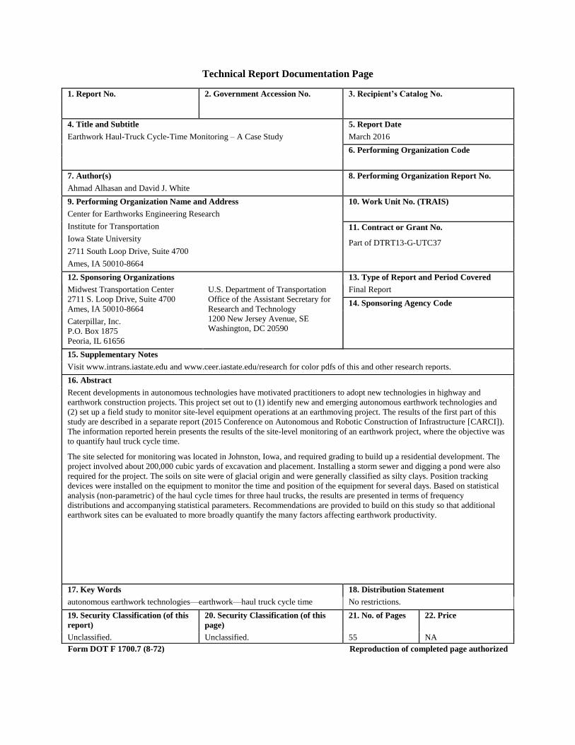
Recent developments in autonomous technologies have motivated practitioners to adopt new technologies in highway and
earthwork construction projects. This project set out to (1) identify new and emerging autonomous earthwork technologies and
(2) set up a field study to monitor site-level equipment operations at an earthmoving project. The results of the first part of this
study are described in a separate report (2015 Conference on Autonomous and Robotic Construction of Infrastructure [CARCI]).
The information reported herein presents the results of the site-level monitoring of an earthwork project, where the objective was
to quantify haul truck cycle time.
The site selected for monitoring was located in Johnston, Iowa, and required grading to build up a residential development. The
project involved about 200,000 cubic yards of excavation and placement. Installing a storm sewer and digging a pond were also
required for the project. The soils on site were of glacial origin and were generally classified as silty clays. Position tracking
devices were installed on the equipment to monitor the time and position of the equipment for several days. Based on statistical
analysis (non-parametric) of the haul cycle times for three haul trucks, the results are presented in terms of frequency
distributions and accompanying statistical parameters. Recommendations are provided to build on this study so that additional
earthwork sites can be evaluated to more broadly quantify the many factors affecting earthwork productivity.
17. Key Words 18. Distribution Statement
autonomous earthwork technologies—earthwork—haul truck cycle time No restrictions.
19. Security Classification (of this
report)
20. Security Classification (of this
page)
21. No. of Pages 22. Price
Unclassified. Unclassified. 55 NA
Form DOT F 1700.7 (8-72) Reproduction of completed page authorized

EARTHWORK HAUL-TRUCK CYCLE-TIME
MONITORING – A CASE STUDY
Final Report
March 2016
Principal Investigator
David J. White
R. L. Handy Professor of Civil Engineering
Center for Earthworks Engineering Research, Iowa State University
Research Assistant
Ahmad Alhasan
Postdoctoral Research Assistant
Center for Earthworks Engineering Research, Iowa State University
Authors
Ahmad Alhasan and David J. White
Sponsored by
Caterpillar, Inc.,
the Midwest Transportation Center, and
the U.S. Department of Transportation
Office of Assistant Secretary for Research and Technology
A report from
Institute for Transportation
Iowa State University
2711 South Loop Drive, Suite 4700
Ames, IA 50010-8664
Phone: 515-294-8103
Fax: 515-294-0467
www.intrans.iastate.edu

v
TABLE OF CONTENTS
ACKNOWLEDGMENTS ............................................................................................................. ix
EXECUTIVE SUMMARY ........................................................................................................... xi
INTRODUCTION ...........................................................................................................................1
BACKGROUND .............................................................................................................................2
PROJECT DETAILS .......................................................................................................................5
POSITION MONITORING RESULTS ........................................................................................12
CYCLE TIME ANALYSIS ...........................................................................................................25
SUMMARY ...................................................................................................................................36
RECOMMENDATIONS FOR FUTURE RESEARCH ................................................................37
REFERENCES ..............................................................................................................................41
vi
LIST OF FIGURES
Figure 1. Idealized cut/fill/haul details for the project .....................................................................5 Figure 2. Equipment monitored on site: CAT D8T bulldozer (top), CAT 375 Hydraulic
Excavator and CAT 740 B truck (center), and Volvo A40F truck (bottom) .......................6
Figure 3. Excavation of the pond (middle left area of image) .........................................................7 Figure 4. Glacial till soil placed in fill area .....................................................................................7 Figure 5. Wet unstable areas of fill that required lime stabilization ................................................8 Figure 6. Wet unstable areas of fill that required lime stabilization, and load of lime ready
for incorporation into soil ....................................................................................................8
Figure 7. Section of haul road observed to pump and rut under haul truck operations ...................9 Figure 8. View from bottom of pond area showing the area being excavated and loaded
into haul trucks .....................................................................................................................9
Figure 9. Loaded CAT 740B haul truck traveling on haul road to fill area ...................................10 Figure 10. AMG CAT D8T bulldozer operations to spread fill ....................................................10 Figure 11. Dewatering operation for pond area and loaded haul truck on haul road ....................11
Figure 12. CAT D8T bulldozer operations for October 17 through October 21 ...........................12 Figure 13. CAT D8T bulldozer operations for October 17 ...........................................................13
Figure 14. CAT D8T bulldozer operations for October 18 ...........................................................13 Figure 15. CAT D8T bulldozer operations for October 19 ...........................................................14 Figure 16. CAT D8T bulldozer operations for October 20 ...........................................................14
Figure 17. CAT D8T bulldozer operations for October 21 ...........................................................15 Figure 18. CAT 375 excavator operations for October 17 through October 19 ............................16
Figure 19. CAT 375 excavator operations for October 17 ............................................................16 Figure 20. CAT 375 excavator operations for October 18 ............................................................17
Figure 21. CAT 375 excavator operations for October 19 ............................................................17 Figure 22. CAT 740B haul truck (#70075) operations for October 17 through October 20 .........18
Figure 23. CAT 740B haul truck (#70075) operations for October 17 .........................................18 Figure 24. CAT 740B haul truck (#70075) operations for October 18 .........................................19 Figure 25. CAT 740B haul truck (#70075) operations for October 19 .........................................19
Figure 26. CAT 740B haul truck (#70075) operations for October 20 .........................................20 Figure 27. Vovlo A40F haul truck operations for October 17 through October 19 ......................20
Figure 28. Vovlo A40F haul truck operations for October 17 .......................................................21 Figure 29. Vovlo A40F haul truck operations for October 18 .......................................................21
Figure 30. Vovlo A40F haul truck operations for October 19 .......................................................22 Figure 31. CAT 740B haul truck (#70073) operations for October 17 through October 20 .........22 Figure 32. CAT 740B haul truck (#70073) operations for October 17 .........................................23 Figure 33. CAT 740B haul truck (#70073) operations for October 18 .........................................23
Figure 34. CAT 740B haul truck (#70073) operations for October 19 .........................................24 Figure 35. CAT 740B haul truck (#70073) operations for October 20 .........................................24 Figure 36. Distribution of cycle times with and without stoppage delays for CAT 740B
haul truck (#70073) ............................................................................................................26 Figure 37. Distribution of cycle times with and without stoppage delays for CAT 740B
haul truck (#70075) ............................................................................................................27 Figure 38. Distribution of cycle times with and without stoppage delays for Volvo A40F
haul truck ...........................................................................................................................28
vii
Figure 39. Comparison of cycle times with and without stoppage delays for all three trucks
on October 17 .....................................................................................................................29 Figure 40. Comparison of cycle times with and without stoppage delays for all three trucks
on October 18 .....................................................................................................................30
Figure 41. Comparison of cycle times with and without stoppage delays for all three trucks
on October 19 .....................................................................................................................31 Figure 42. Comparison of estimated production rates of three haul trucks, October 17 ...............32 Figure 43. Comparison of estimated production rates of three haul trucks, October 18 ...............33 Figure 44. Comparison of estimated production rates of three haul trucks, October 19 ...............34
Figure 45. Parameters and interconnectivity of parameters that relate to earthwork
productivity ........................................................................................................................38 Figure 46. Schematic of the dynamic regression model for future productivity analysis .............40
LIST OF TABLES
Table 1. List of equipment monitored on site ..................................................................................5


ix
ACKNOWLEDGMENTS
The authors would like to thank Caterpillar, Inc.; the Midwest Transportation Center; and the
U.S. Department of Transportation Office of the Assistant Secretary for Research and
Technology for sponsoring this research.
The authors would also like to thank McAninch Corporation for allowing the research team
access to the project site to carry out the field monitoring phase of this project.

xi
EXECUTIVE SUMMARY
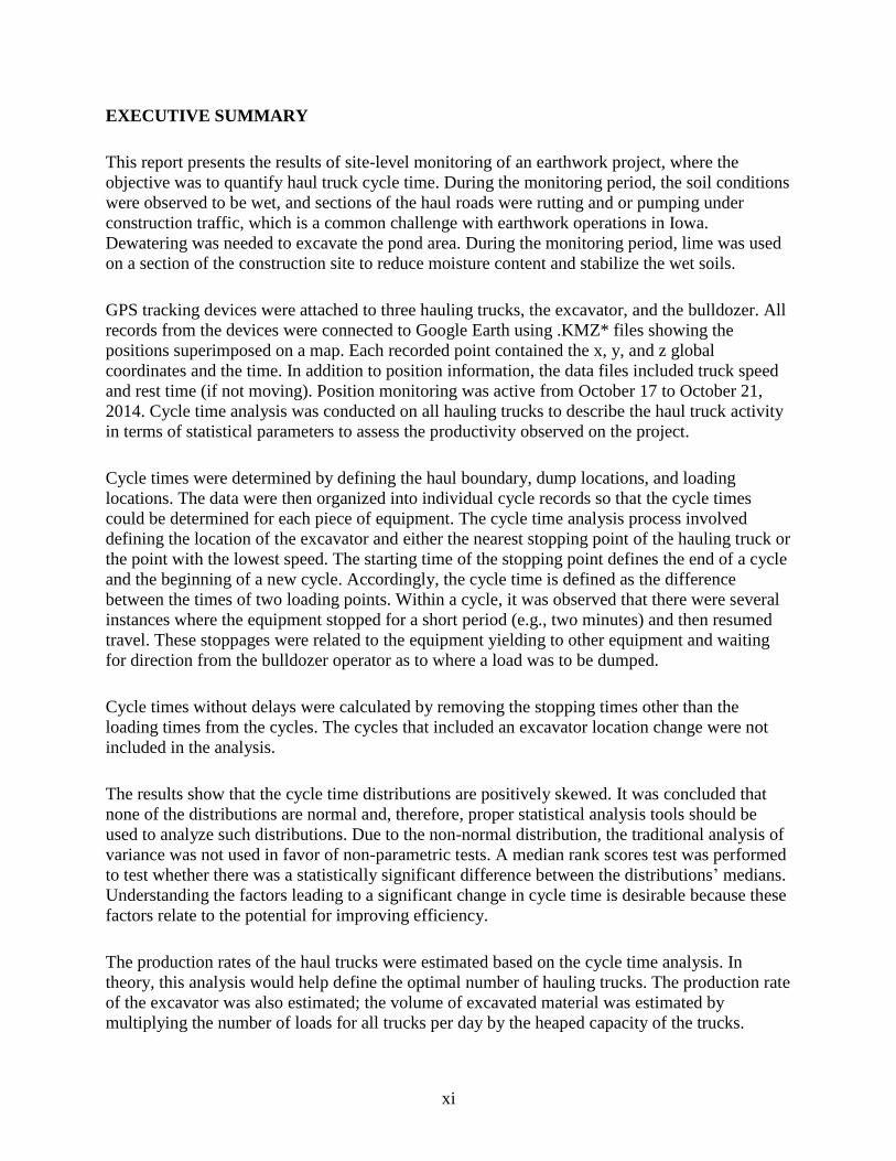
This report presents the results of site-level monitoring of an earthwork project, where the
objective was to quantify haul truck cycle time. During the monitoring period, the soil conditions
were observed to be wet, and sections of the haul roads were rutting and or pumping under
construction traffic, which is a common challenge with earthwork operations in Iowa.
Dewatering was needed to excavate the pond area. During the monitoring period, lime was used
on a section of the construction site to reduce moisture content and stabilize the wet soils.
GPS tracking devices were attached to three hauling trucks, the excavator, and the bulldozer. All
records from the devices were connected to Google Earth using .KMZ* files showing the
positions superimposed on a map. Each recorded point contained the x, y, and z global
coordinates and the time. In addition to position information, the data files included truck speed
and rest time (if not moving). Position monitoring was active from October 17 to October 21,
2014. Cycle time analysis was conducted on all hauling trucks to describe the haul truck activity
in terms of statistical parameters to assess the productivity observed on the project.
Cycle times were determined by defining the haul boundary, dump locations, and loading
locations. The data were then organized into individual cycle records so that the cycle times
could be determined for each piece of equipment. The cycle time analysis process involved
defining the location of the excavator and either the nearest stopping point of the hauling truck or
the point with the lowest speed. The starting time of the stopping point defines the end of a cycle
and the beginning of a new cycle. Accordingly, the cycle time is defined as the difference
between the times of two loading points. Within a cycle, it was observed that there were several
instances where the equipment stopped for a short period (e.g., two minutes) and then resumed
travel. These stoppages were related to the equipment yielding to other equipment and waiting
for direction from the bulldozer operator as to where a load was to be dumped.
Cycle times without delays were calculated by removing the stopping times other than the
loading times from the cycles. The cycles that included an excavator location change were not
included in the analysis.
The results show that the cycle time distributions are positively skewed. It was concluded that
none of the distributions are normal and, therefore, proper statistical analysis tools should be
used to analyze such distributions. Due to the non-normal distribution, the traditional analysis of
variance was not used in favor of non-parametric tests. A median rank scores test was performed
to test whether there was a statistically significant difference between the distributions’ medians.
Understanding the factors leading to a significant change in cycle time is desirable because these
factors relate to the potential for improving efficiency.
The production rates of the haul trucks were estimated based on the cycle time analysis. In
theory, this analysis would help define the optimal number of hauling trucks. The production rate
of the excavator was also estimated; the volume of excavated material was estimated by
multiplying the number of loads for all trucks per day by the heaped capacity of the trucks.

xii
This study served to demonstrate a relatively simple approach to cycle time monitoring and
statistical analysis. However, more advanced data collection and analysis are needed. Moving
forward, a more completely designed monitoring program should be devised to capture the
effects of the many factors that can influence productivity. For future site-level monitoring
programs, an emphasis needs to be placed on carefully capturing and quantifying the key
parameters influencing productivity. There is very limited published information on this topic.
Future studies should consider the following parameters at minimum to build a site-level analysis
model:
Project complexity (i.e., site layout and details)
Dump truck size
Number of dump trucks
Loader size
Number of loaders
Excavation rates
Material transfer rates
Machines’ paths and traffic (i.e., speed, location, and time)
Haul road resistance
Work zone drainage
Soil condition

1
INTRODUCTION
Recent developments in autonomous technologies have motivated practitioners to adopt new
technologies in highway and earthwork construction projects. Automated machine guidance
(AMG) is one example that improves earthwork productivity by linking sophisticated design
software with construction equipment to direct the operations of construction machinery with a
high level of precision, which improves construction efficiency and quality (Vennapusa et al.
2015). AMG includes various technologies (e.g., GPS guidance, three-dimensional [3D]
modeling, and machine control) implemented at both the planning and construction stages.
To identify new and emerging technologies that will go beyond AMG in the construction
automation space, the current project set out to (1) identify current research and development
efforts by hosting a conference of world-wide experts and (2) set up a field study to monitor site-
level equipment operations at an earthmoving project to better identify opportunities for
integrating automation into the process. The information reported herein presents the results of
the site-level monitoring of an earthwork project. The results of the conference are described in
White et al. (2015) and are briefly summarized in the following.
The 2015 Conference on Autonomous and Robotic Construction of Infrastructure (CARCI)
(White et al. 2015) was attended by more than 100 participants from academia and industry and
showed that new construction applications for autonomous/robotic systems are rapidly emerging.
Topics presented at the CARCI conference include mobile robotic operations, advanced visual
analysis, terrain modeling, simulation, multi-dimensional modeling, 3D printing/manufacturing,
data processing, and 3D point cloud generation from digital imagery and other measurement
technologies. Twenty-one papers are published in the proceedings and are available online at
http://www.ceer.iastate.edu/CARCI/proceedings/.
The success of the CARCI conference confirmed the wide ranging interest in further automating
construction processes and brought attention to the need for detailed site-level monitoring
research to better identify opportunities for further advancements in autonomous, robotic, and
co-robotic operations for earthwork and infrastructure construction work. The study described
herein offers new information about a relatively simple haul truck monitoring program with
relatively inexpensive monitoring equipment and further lays the groundwork for more advanced
studies in this area, which are necessary because of the rather complex number of parameters
involved and the lack of a quantified framework for assessing earthwork productivity problems.
2
BACKGROUND
AMG applications in earthwork grading operations are now well integrated into practice and
represent an excellent example of how new technology has found a market due to the improved
productivity and profitability that it offers users.
Hannon (2007) stated that AMG technologies have proven their value in the field but also noted
that there is a need for continued standardization to specify the proper use of various AMG and
related technologies. Other studies have reported productivity gains and cost savings when
utilizing AMG technologies (Aðalsteinsson 2008, Capony et al. 2012, Hammad et al. 2012,
Jonasson et al. 2002).
Early developments in manufacturing automation have motivated researchers to identify the
difference between automation in the manufacturing and construction industries. Everett and
Slocum (1994) indicated that approaches to automation in manufacturing cannot be transferred to
construction, and instead construction must develop its own strategies. They also indicated that
machines excel at physically intensive basic tasks that require speed, strength, repetitive motions,
and operation in hostile environments. Though human craft workers are still more productive and
cost effective than machines and computers for basic information-intensive tasks, this situation
might be changing with rapid improvements in machine awareness (Steward et al. 2015).
Different construction automation technologies have been developed based on specific activities
of interest. Olearczyk et al. (2014) introduced a Crane Lifting Path Planning (CLPP) algorithm
that utilizes a piecewise continuous function in terms of the rotation angle and translation
(radius) of the boom to reduce the complexity of the system of equations when optimizing the
crane path. Liu et al. (2013) developed an automated system to control the watering operations of
dam materials according to the volume and type of material carried in a truck. This system
facilitates obtaining an optimal moisture content for these materials efficiently, thus ensuring the
compaction efficiency of earth-rock dam construction.
Furthermore, new autonomous paving systems have been developed. These systems can increase
the efficiency and quality of operations, lead to reductions in overall project costs and time, and
enhance pavement life (Krishnamurthy et al. 1998). Krishnamurthy et al. (1998) introduced a
new system, named AUTOPAVE (v1.0), that utilizes algorithmic planning and real-time
guidance strategies for semi-automated path-planning and real-time guidance.
Earthworks are complex activities in nature due to the variability in site conditions, project
designs, and soil conditions, among other variables, all of which requires specialized AMG
systems. Santos et al. (2000) developed a framework to control autonomous backhoe-type
excavators. In their study, the control structure was divided into low and high levels. The low-
level control utilized fuzzy logic to encapsulate expert experience for capturing soil properties in
many excavation scenarios. Unified modelling language (UML) statecharts were used at the
higher level for mapping environment and machine sensor data to actuator control signals. The
mapping was based on a deep understanding of excavation performed by a skillful operator and
was coded into rule sets. Cannon and Singh (2000) introduced a composite forward model of the
3
mechanics of a backhoe excavator digging in soil. The model predicts the excavator’s trajectory
based on estimations of soil properties and predicts contact forces between the excavator and the
terrain.
Stentz et al. (1999) developed a system that enables the excavator to decide where to dig in the
soil, where to dump the materials carried in the truck, and how to quickly move between points
while detecting and stopping for obstacles. The system included two scanning laser rangefinders
to recognize and localize the truck, measure the soil face, and detect obstacles and included
software capable of analyzing the inputs and controlling the operation. The system was fully
implemented and was demonstrated to load trucks as fast as human operators. Capony et al.
(2012) reported that the use of GPS-equipped excavators can achieve more accurate earthwork
operations and reduce fuel consumption and working time.
AMG requires advanced planning technologies to provide digital plans that are compatible with
the control systems during construction. Jayawardane and Harris (1990) utilized linear
programming to optimize a comprehensive earthmoving system in road construction by
comparing alternative fleets (from among different available fleets) to provide an optimum
material distribution and recommend appropriate plant fleets to complete a project within the
specified time. Further developments in computer knowledge–based simulations have allowed
automated earthmoving project planning (Askew et al. 2002).
Building information modeling (BIM) and multidimensional modeling simulations are more
appropriate tools developed for planning and AMG applications. Huang and Bernold (1997)
developed a computer-aided design (CAD) integrated with trenching and pipe-laying machines.
The system could lay the foundation for safer and more productive trenching operations in the
future. Ji et al. (2009) presented a framework to conduct simulations of earthwork operations
using a 3D roadway model, 3D surface model, and 3D subsoil model. The simulation was based
on the discrete events paradigm, which describes entities such as diggers and trucks, their
behavior, and the time required for an atomic process step. The results provided information on
the utilization ratio of the employed resources and the time required for completing the entire
earthwork project.
Kamat and Martinez (2001, 2003) described the methodology and a first version of a general
purpose 3D visualization system (i.e., Dynamic Construction Visualizer), which is a discrete
event construction simulation that is independent of CAD software. This system enables spatially
and chronologically accurate 3D visualization of modeled construction operations and the
resulting products. Miller et al. (2011) utilized 3D models to visualize paving jobs and help
understand the relationship between machine operations and hot-mix asphalt (HMA) temperature
and the impact of this relationship on HMA compaction.
BIM use has grown rapidly in recent years due to its usefulness for geometric modelling of a
building’s performance and for its benefits in terms of cost reduction, the control it provides
throughout the project’s lifecycle, and significant time savings (Barlish and Sullivan 2012, Bryde
et al. 2013). Eadie et al. (2013) reported some issues that limit the use of BIM, such as lack of
expertise within the project team, cultural resistance (Dawood and Iqbal 2010, Denzer and

4
Hedges 2008), resistance at the operational level (Bender 2010), lack of immediate benefits from
projects delivered to date (Sebastian 2010), legal issues regarding ownership, and insurance
(Chynoweth et al. 2007, Olatunji 2011, Race 2012).
Goodrum (2001) discussed an approach to quantifying the effects of construction technology on
labor and partial-factor productivity. Other researchers have implemented machine learning
approaches to define different factors related to project productivity (AbouRizk et al. 2001,
Heravi and Eslamdoost 2015, Hola and Schabowicz 2010). Although many studies have
investigated the effects of different parameters on project productivity at the activity level, fewer
studies have modeled the relationship between AMG and construction productivity factors and
parameters. The present study introduces a case study using AMG-equipped machines. The data
provided are limited to GPS monitoring data to investigate the cycle times of hauling trucks
during earthwork activities.

5
PROJECT DETAILS
The site selected for monitoring was located in Johnston, Iowa, and required grading to build up
a residential development. The project involved about 200,000 cubic yards of excavation and
placement. Installing a storm sewer and digging a pond were also required for the project. The
soils on site were of glacial origin and were generally classified as silty clays. Project monitoring
occurred in October 2014. Figure 1 shows the simplified site plan and highlights the primary
haul road, the primary fill area, and the pond excavation area.
Figure 1. Idealized cut/fill/haul details for the project
Table 1 summarizes the equipment used on site during the monitoring phase of the project.
Table 1. List of equipment monitored on site
Equipment Model Number Name
Max. Heaped
Capacity (yd3)
Excavator Caterpillar (CAT) 375
Hydraulic Excavator
Excavator 7.0
Hauling truck CAT 740 B CAT 70073 31.4
Hauling truck CAT 740 B CAT 70075 31.4
Hauling truck Volvo A40F Volvo 31.4
Bulldozer CAT D8T Bulldozer 6.1
Figure 2 shows the equipment.
6
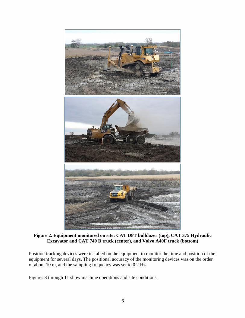
Figure 2. Equipment monitored on site: CAT D8T bulldozer (top), CAT 375 Hydraulic
Excavator and CAT 740 B truck (center), and Volvo A40F truck (bottom)
Position tracking devices were installed on the equipment to monitor the time and position of the
equipment for several days. The positional accuracy of the monitoring devices was on the order
of about 10 m, and the sampling frequency was set to 0.2 Hz.
Figures 3 through 11 show machine operations and site conditions.
7
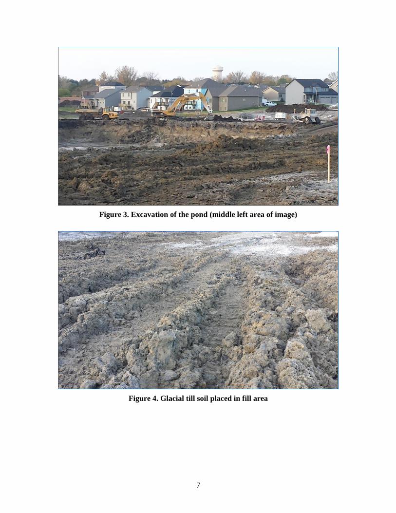
Figure 3. Excavation of the pond (middle left area of image)
Figure 4. Glacial till soil placed in fill area

8
Figure 5. Wet unstable areas of fill that required lime stabilization
Figure 6. Wet unstable areas of fill that required lime stabilization, and load of lime ready
for incorporation into soil
9
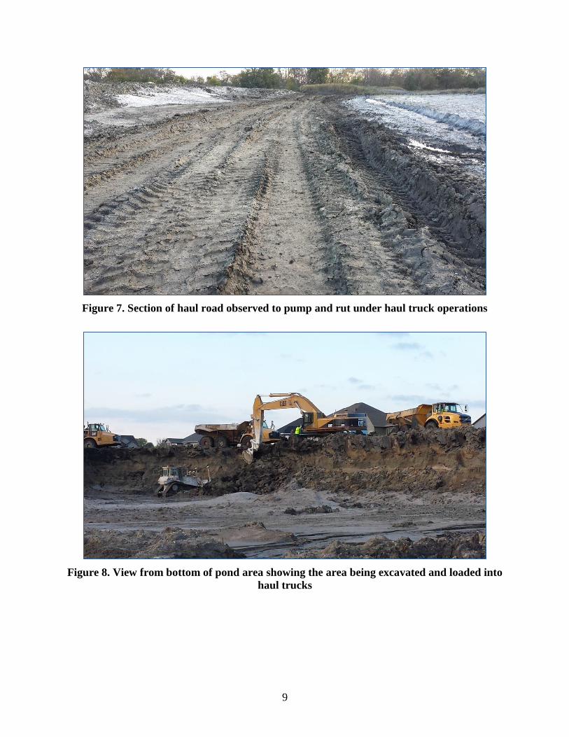
Figure 7. Section of haul road observed to pump and rut under haul truck operations
Figure 8. View from bottom of pond area showing the area being excavated and loaded into
haul trucks
10
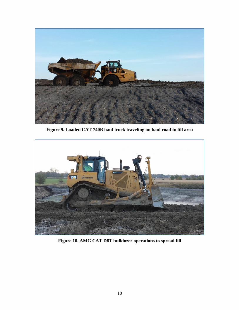
Figure 9. Loaded CAT 740B haul truck traveling on haul road to fill area
Figure 10. AMG CAT D8T bulldozer operations to spread fill
11
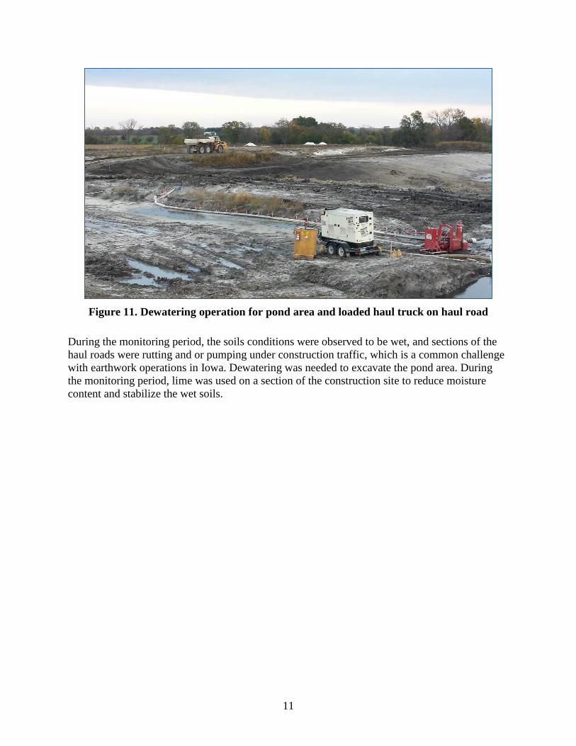
Figure 11. Dewatering operation for pond area and loaded haul truck on haul road
During the monitoring period, the soils conditions were observed to be wet, and sections of the
haul roads were rutting and or pumping under construction traffic, which is a common challenge
with earthwork operations in Iowa. Dewatering was needed to excavate the pond area. During
the monitoring period, lime was used on a section of the construction site to reduce moisture
content and stabilize the wet soils.
12
POSITION MONITORING RESULTS
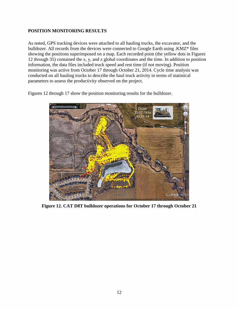
As noted, GPS tracking devices were attached to all hauling trucks, the excavator, and the
bulldozer. All records from the devices were connected to Google Earth using .KMZ* files
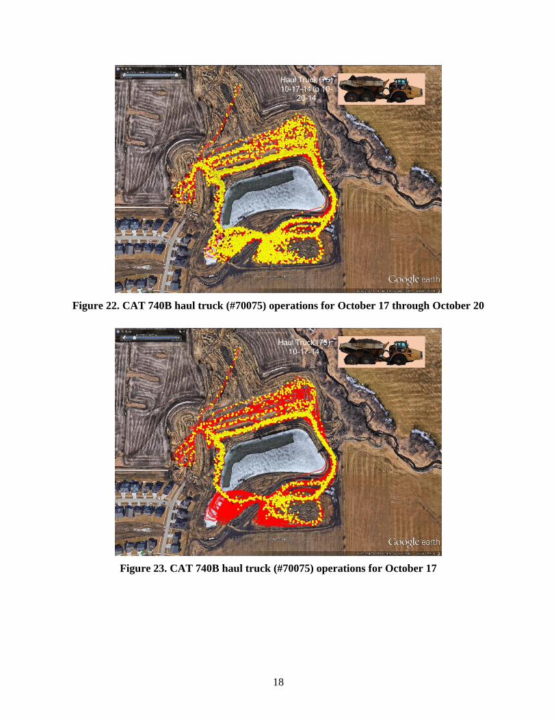
showing the positions superimposed on a map. Each recorded point (the yellow dots in Figures
12 through 35) contained the x, y, and z global coordinates and the time. In addition to position
information, the data files included truck speed and rest time (if not moving). Position
monitoring was active from October 17 through October 21, 2014. Cycle time analysis was
conducted on all hauling trucks to describe the haul truck activity in terms of statistical
parameters to assess the productivity observed on the project.
Figures 12 through 17 show the position monitoring results for the bulldozer.
Figure 12. CAT D8T bulldozer operations for October 17 through October 21

13
Figure 13. CAT D8T bulldozer operations for October 17
Figure 14. CAT D8T bulldozer operations for October 18
14
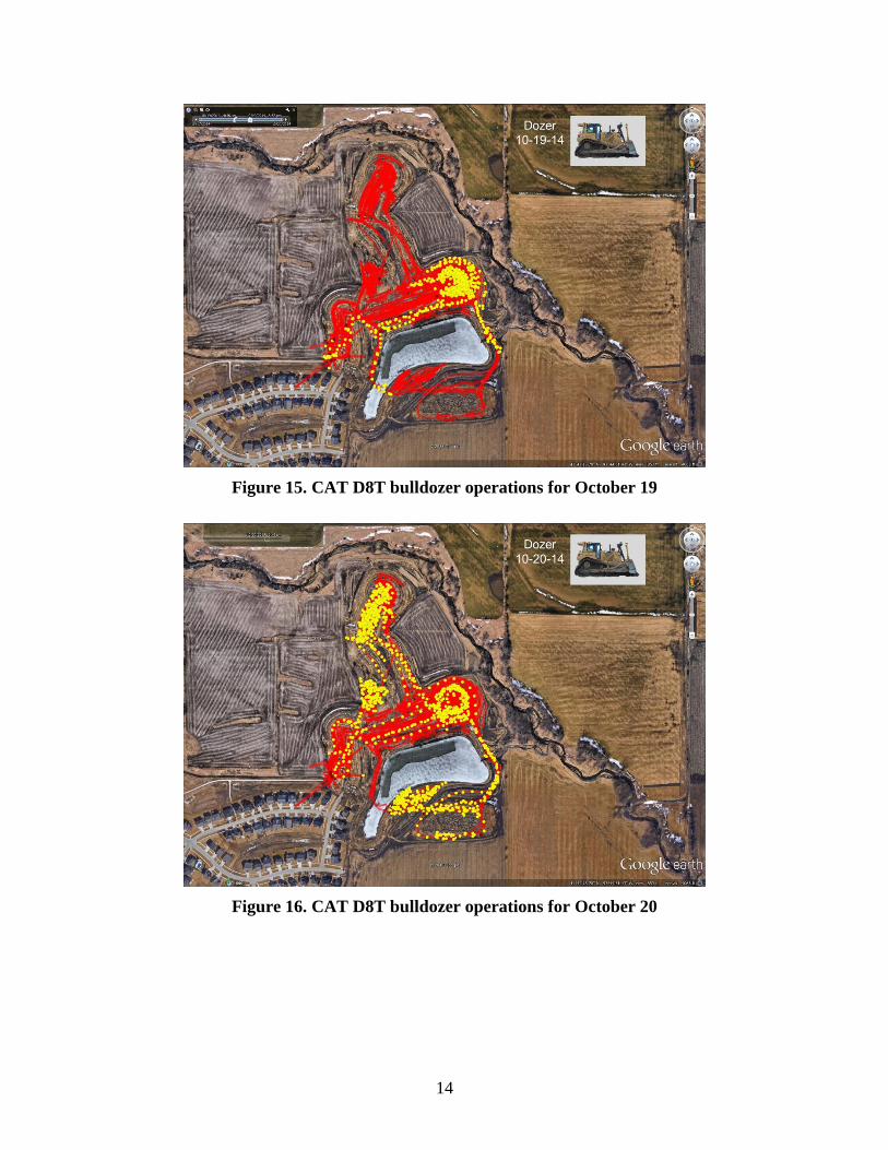
Figure 15. CAT D8T bulldozer operations for October 19
Figure 16. CAT D8T bulldozer operations for October 20
15
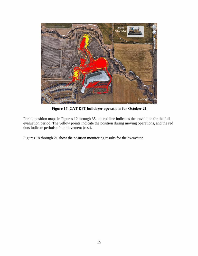
Figure 17. CAT D8T bulldozer operations for October 21
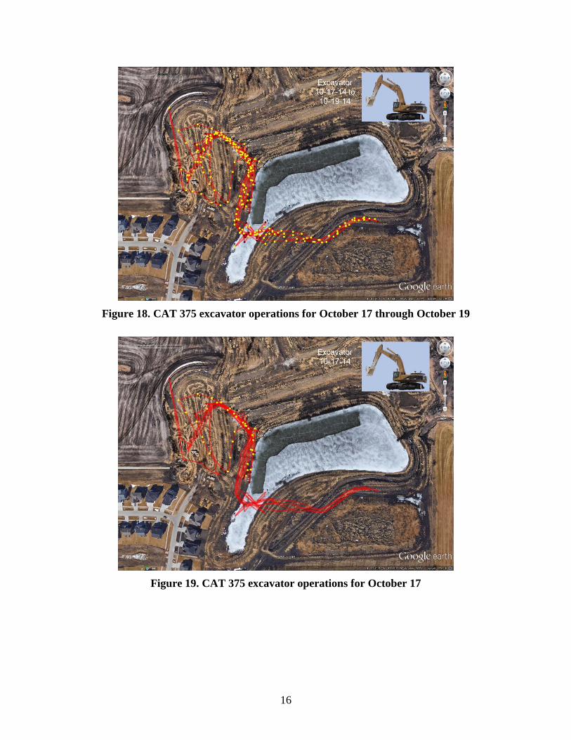
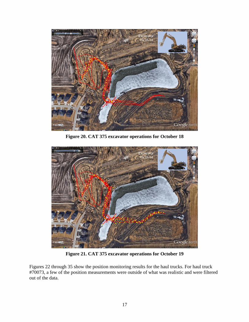
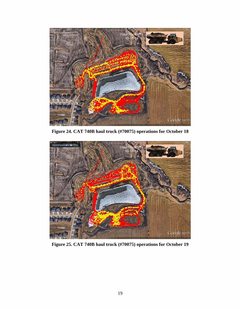
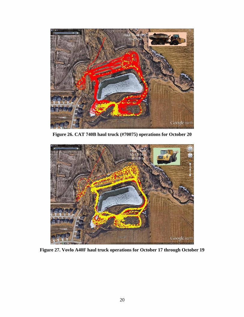
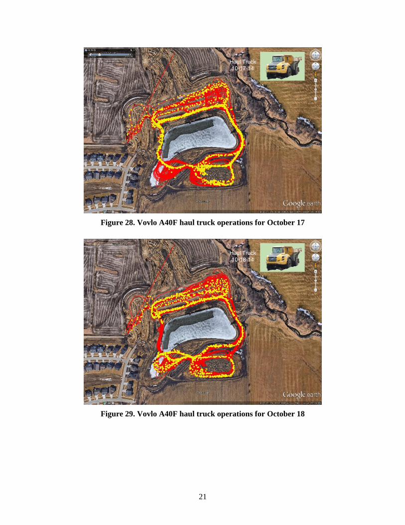
For all position maps in Figures 12 through 35, the red line indicates the travel line for the full
evaluation period. The yellow points indicate the position during moving operations, and the red
dots indicate periods of no movement (rest).
Figures 18 through 21 show the position monitoring results for the excavator.
16
Figure 18. CAT 375 excavator operations for October 17 through October 19
Figure 19. CAT 375 excavator operations for October 17
17
Figure 20. CAT 375 excavator operations for October 18
Figure 21. CAT 375 excavator operations for October 19
Figures 22 through 35 show the position monitoring results for the haul trucks. For haul truck
#70073, a few of the position measurements were outside of what was realistic and were filtered
out of the data.
18
Figure 22. CAT 740B haul truck (#70075) operations for October 17 through October 20
Figure 23. CAT 740B haul truck (#70075) operations for October 17
19
Figure 24. CAT 740B haul truck (#70075) operations for October 18
Figure 25. CAT 740B haul truck (#70075) operations for October 19
20
Figure 26. CAT 740B haul truck (#70075) operations for October 20
Figure 27. Vovlo A40F haul truck operations for October 17 through October 19
21
Figure 28. Vovlo A40F haul truck operations for October 17
Figure 29. Vovlo A40F haul truck operations for October 18
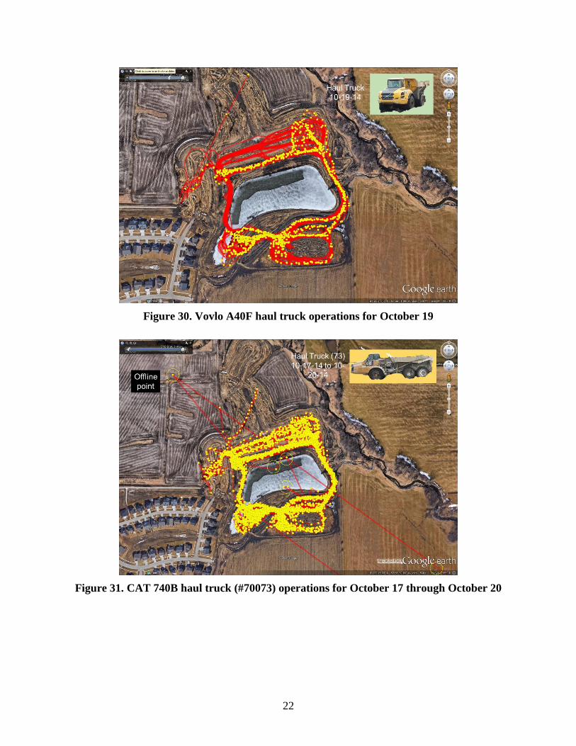
22
Figure 30. Vovlo A40F haul truck operations for October 19
Figure 31. CAT 740B haul truck (#70073) operations for October 17 through October 20
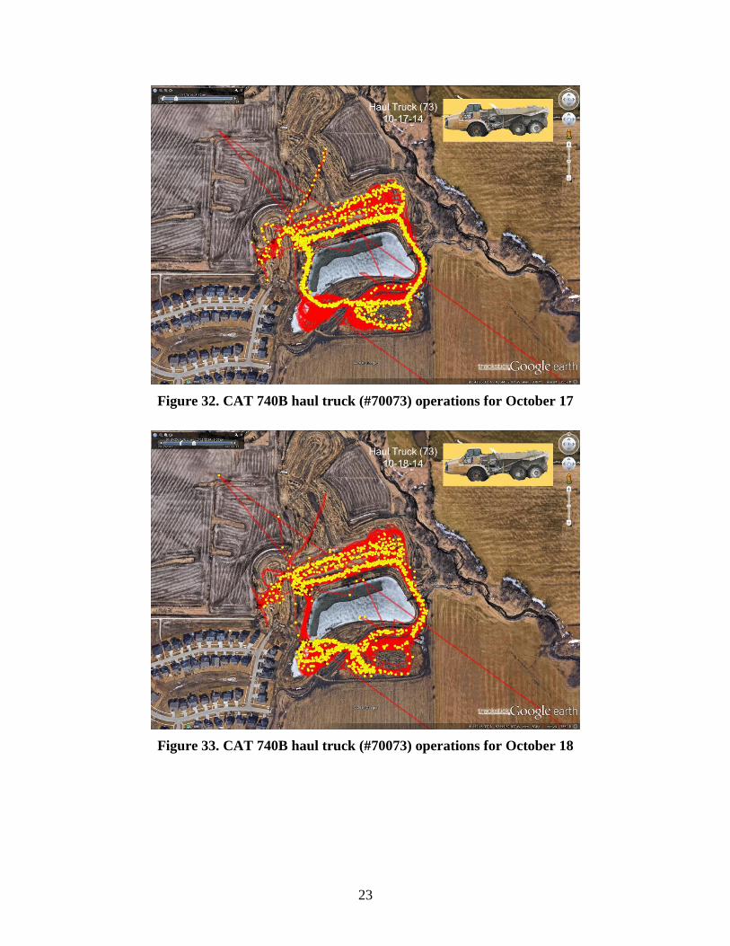
23
Figure 32. CAT 740B haul truck (#70073) operations for October 17
Figure 33. CAT 740B haul truck (#70073) operations for October 18
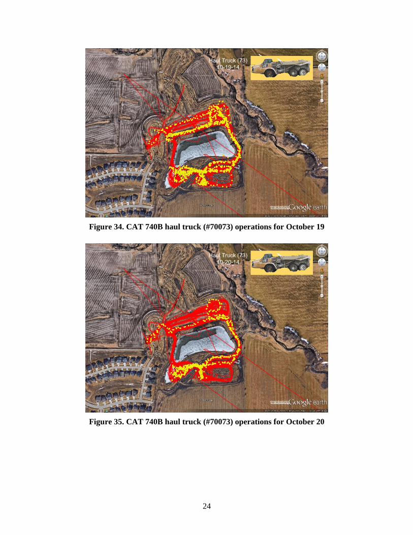
24
Figure 34. CAT 740B haul truck (#70073) operations for October 19
Figure 35. CAT 740B haul truck (#70073) operations for October 20

25
CYCLE TIME ANALYSIS
One of the goals of this project was to make use of relatively inexpensive GPS positing
equipment to generate data for equipment cycle time monitoring and analysis. Cycle times were
determined by defining the haul boundary, dump locations, and loading locations. The data were
then organized into individual cycle records so that the cycle times could be determined for each
piece of equipment.
The cycle time analysis process involved defining the location of the excavator and either the
nearest stopping point of the hauling truck or the point with the lowest speed. The starting time
of the stopping point defines the end of a cycle and the beginning of a new cycle. Accordingly,
the cycle time is defined as the difference between the times of two loading points. Within a
cycle, it was observed that there were several instances where the equipment stopped for a short
period (e.g., two minutes) and then resumed travel. These stoppages were related to the
equipment yielding to other equipment and waiting for direction from the bulldozer operator as
to where a load was to be dumped.
Cycle times without delays were calculated by removing the stopping times other than the
loading times from the cycles. The cycles that included an excavator location change were not
included in the analysis.
Figure 36 shows a histogram of the cycle times for one of the haul trucks during the monitoring
period.
26
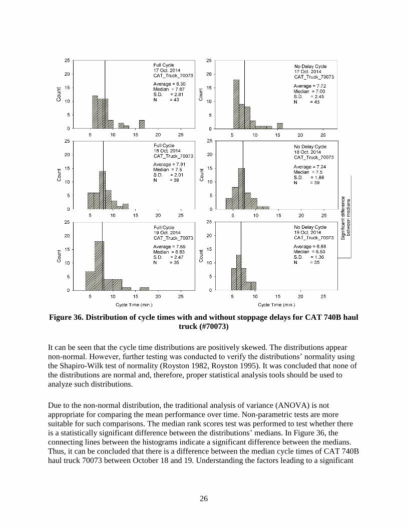
Figure 36. Distribution of cycle times with and without stoppage delays for CAT 740B haul
truck (#70073)
It can be seen that the cycle time distributions are positively skewed. The distributions appear
non-normal. However, further testing was conducted to verify the distributions’ normality using
the Shapiro-Wilk test of normality (Royston 1982, Royston 1995). It was concluded that none of
the distributions are normal and, therefore, proper statistical analysis tools should be used to
analyze such distributions.
Due to the non-normal distribution, the traditional analysis of variance (ANOVA) is not
appropriate for comparing the mean performance over time. Non-parametric tests are more
suitable for such comparisons. The median rank scores test was performed to test whether there
is a statistically significant difference between the distributions’ medians. In Figure 36, the
connecting lines between the histograms indicate a significant difference between the medians.
Thus, it can be concluded that there is a difference between the median cycle times of CAT 740B
haul truck 70073 between October 18 and 19. Understanding the factors leading to a significant
27
change in cycle time is desirable because these factors relate to the potential for improving
efficiency.
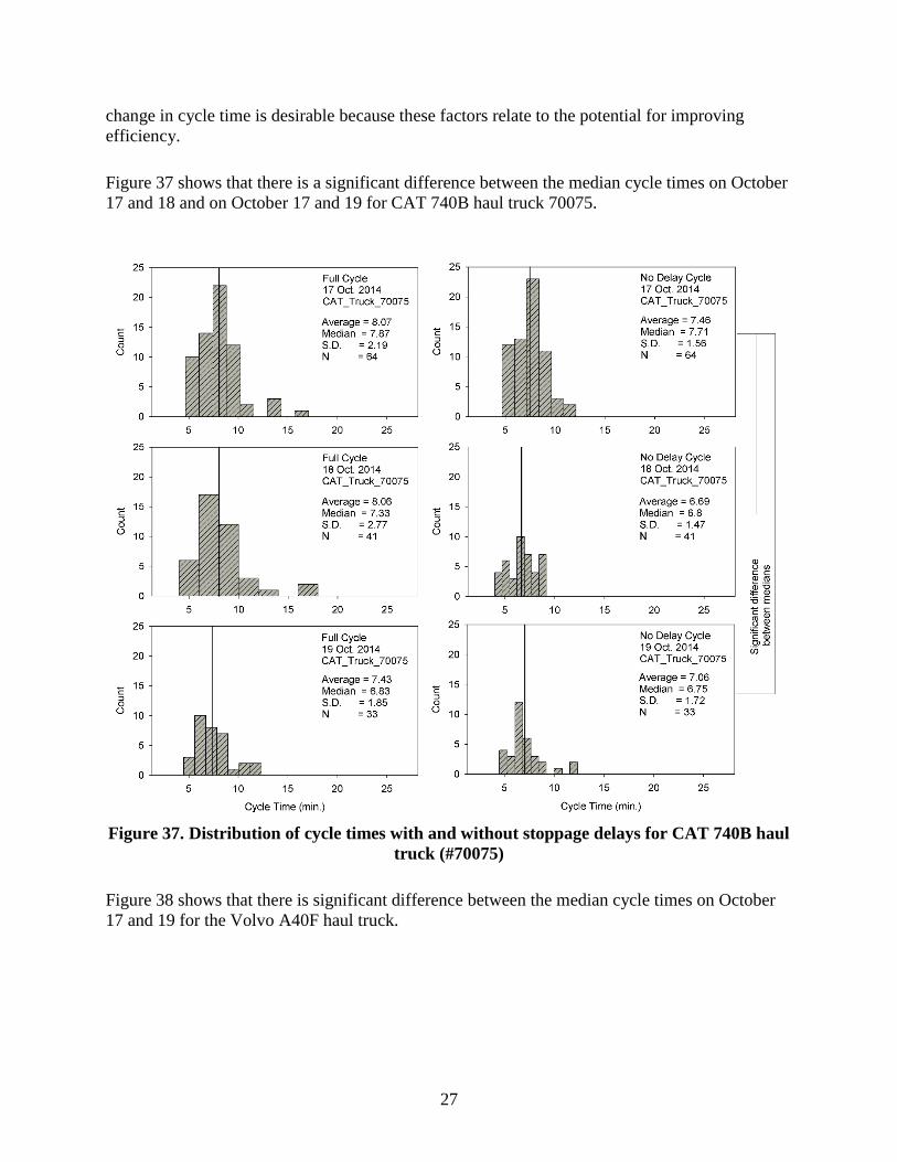
Figure 37 shows that there is a significant difference between the median cycle times on October
17 and 18 and on October 17 and 19 for CAT 740B haul truck 70075.
Figure 37. Distribution of cycle times with and without stoppage delays for CAT 740B haul
truck (#70075)
Figure 38 shows that there is significant difference between the median cycle times on October
17 and 19 for the Volvo A40F haul truck.

28
Figure 38. Distribution of cycle times with and without stoppage delays for Volvo A40F
haul truck
Based on the statistical analysis conducted on the cycle time distributions, it can be stated that
the cycle times were improved (i.e., made shorter) as the monitoring period progressed. This
improvement might be due to the operator’s increasing familiarity with the nature of the site
nature or other factors.
Further median score tests were performed to compare the three trucks’ cycle times on each day
from October 17 to 19. The results are presented in Figures 39 through 41.

29
Figure 39. Comparison of cycle times with and without stoppage delays for all three trucks
on October 17
30
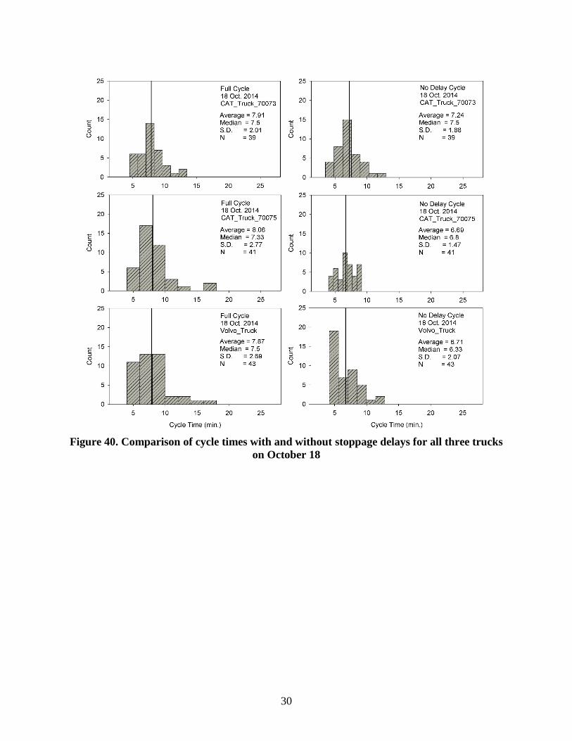
Figure 40. Comparison of cycle times with and without stoppage delays for all three trucks
on October 18
31
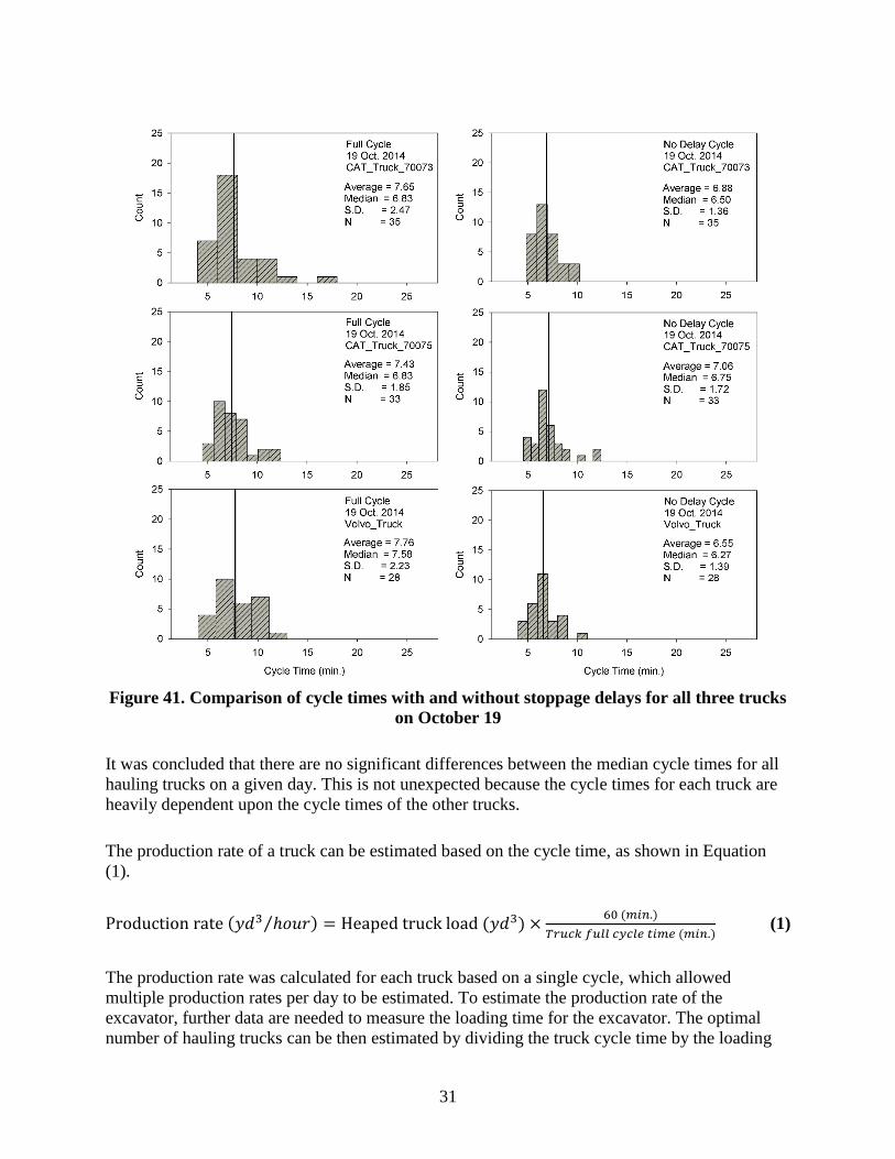
Figure 41. Comparison of cycle times with and without stoppage delays for all three trucks
on October 19
It was concluded that there are no significant differences between the median cycle times for all
hauling trucks on a given day. This is not unexpected because the cycle times for each truck are
heavily dependent upon the cycle times of the other trucks.
The production rate of a truck can be estimated based on the cycle time, as shown in Equation
(1).
Production rate (𝑦𝑑3 ℎ𝑜𝑢𝑟⁄ ) = Heaped truck load (𝑦𝑑3) ×60 (𝑚𝑖𝑛.)
𝑇𝑟𝑢𝑐𝑘 𝑓𝑢𝑙𝑙 𝑐𝑦𝑐𝑙𝑒 𝑡𝑖𝑚𝑒 (𝑚𝑖𝑛.) (1)
The production rate was calculated for each truck based on a single cycle, which allowed
multiple production rates per day to be estimated. To estimate the production rate of the
excavator, further data are needed to measure the loading time for the excavator. The optimal
number of hauling trucks can be then estimated by dividing the truck cycle time by the loading
32
cycle time. One of the two integer values is then assigned as the optimal number based on the
cost.
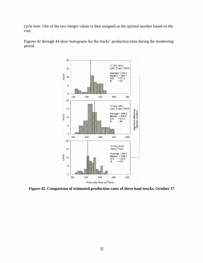
Figures 42 through 44 show histograms for the trucks’ production rates during the monitoring
period.
Figure 42. Comparison of estimated production rates of three haul trucks, October 17
33
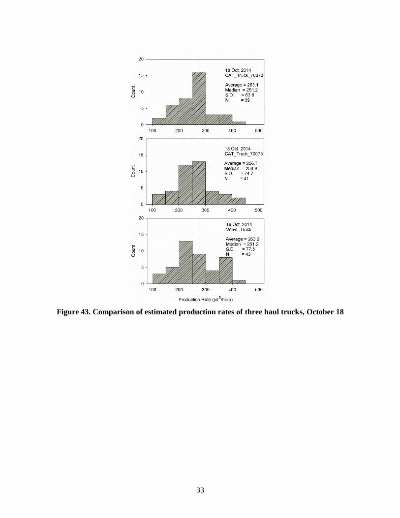
Figure 43. Comparison of estimated production rates of three haul trucks, October 18
34
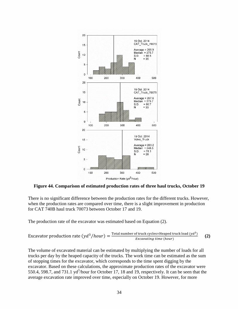
Figure 44. Comparison of estimated production rates of three haul trucks, October 19
There is no significant difference between the production rates for the different trucks. However,
when the production rates are compared over time, there is a slight improvement in production
for CAT 740B haul truck 70073 between October 17 and 19.
The production rate of the excavator was estimated based on Equation (2).
Excavator production rate (𝑦𝑑3 ℎ𝑜𝑢𝑟⁄ ) =Total number of truck cycles×Heaped truck load (𝑦𝑑3)
𝐸𝑥𝑐𝑎𝑣𝑎𝑡𝑖𝑛𝑔 𝑡𝑖𝑚𝑒 (ℎ𝑜𝑢𝑟) (2)
The volume of excavated material can be estimated by multiplying the number of loads for all
trucks per day by the heaped capacity of the trucks. The work time can be estimated as the sum
of stopping times for the excavator, which corresponds to the time spent digging by the
excavator. Based on these calculations, the approximate production rates of the excavator were
550.4, 598.7, and 731.1 yd3/hour for October 17, 18 and 19, respectively. It can be seen that the
average excavation rate improved over time, especially on October 19. However, for more

35
realistic production rates, additional details on the number of cycles for the excavator should be
recorded.
36
SUMMARY
The study of site-level earthwork project monitoring described in this report quantifies haul truck
cycle times. GPS tracking devices were attached to three hauling trucks, the excavator, and the
bulldozer. Each recorded point contained the x, y, and z global coordinates and the time. In
addition to position information, the data files included truck speed and rest time (if not moving).
Cycle time analysis was then conducted to describe the haul truck activity in terms of statistical
parameters. The key findings from this study are as follows:
Cycle times were determined by defining the haul boundary, dump locations, and loading
locations. The data were then organized into individual cycle records so that the cycle times
could be determined for each piece of equipment. The cycle time analysis process involved
defining the location of the excavator and either the nearest stopping point of the hauling
truck or the point with the lowest speed. The starting time of the stopping point defines the
end of a cycle and the beginning of a new cycle. Accordingly, the cycle time is defined as the
difference between the times of two loading points.
Within a cycle, it was observed that there were several instances where the equipment
stopped for a short period (e.g., two minutes) and then resumed travel. These stoppages were
related to the equipment yielding to other equipment and waiting for direction from the
bulldozer operator as to where a load was to be dumped.
Cycle times without delays were calculated by removing the stopping times other than the
loading times from the cycles. The cycles that included an excavator location change were
not included in the analysis.
The results show that the cycle time distributions are positively skewed. It was concluded
that none of the distributions are normal and, therefore, proper statistical analysis tools
should be used to analyze such distributions. Due to the non-normal distribution, the
traditional analysis of variance was not used in favor of non-parametric tests. A median rank
scores test was performed to test whether there was a statistically significant difference
between the distributions’ medians.
Understanding the factors leading to a significant change in cycle time is desirable because
these factors relate to the potential for improving efficiency.
The production rates of the haul trucks were estimated based on the cycle time analysis. In
theory, this analysis would help define the optimal number of hauling trucks. The production
rate of the excavator was also estimated; the volume of excavated material was estimated by
multiplying the number of loads for all trucks per day by the heaped capacity of the trucks.

37
RECOMMENDATIONS FOR FUTURE RESEARCH
This study served to demonstrate a relatively simple approach to cycle time monitoring and
statistical analysis. However, more advanced data collection and analysis are needed. Moving
forward, a more completely designed monitoring program should be devised to capture the
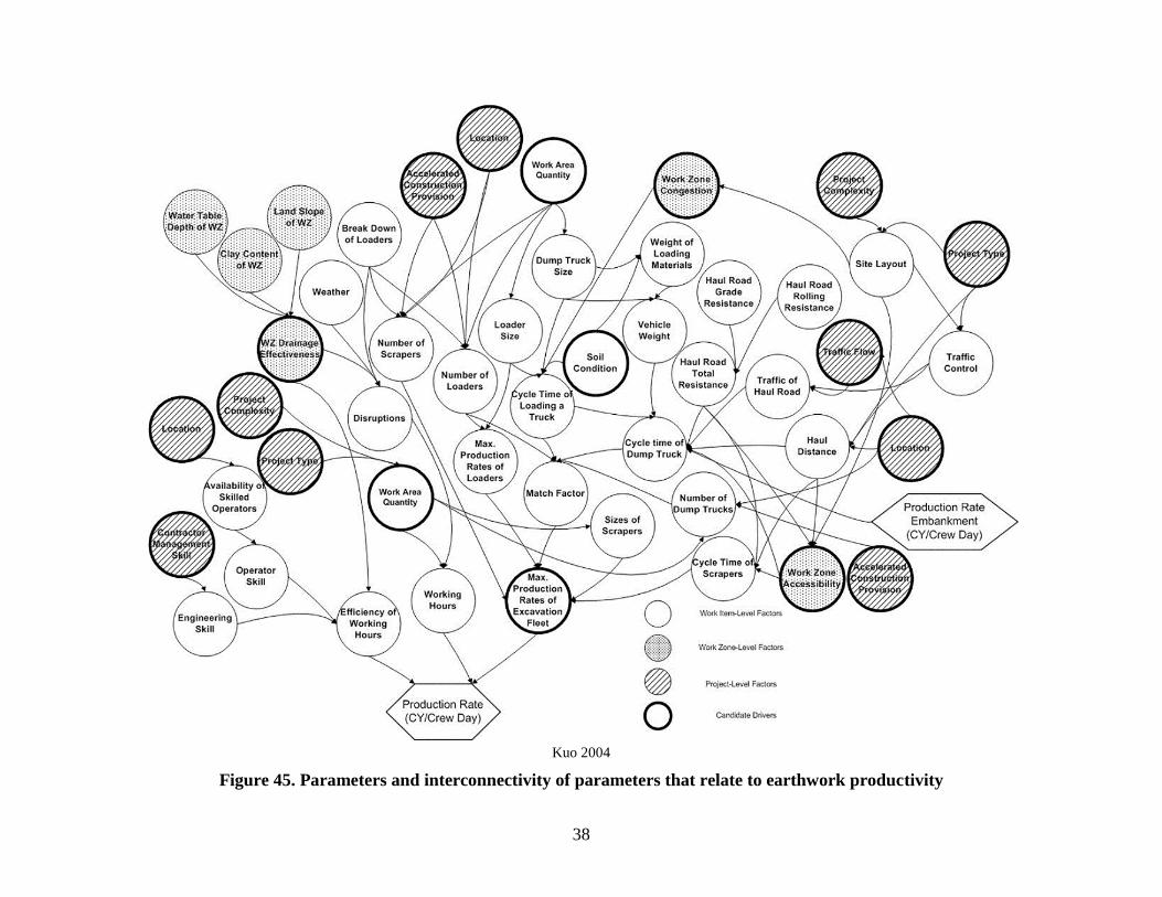
effects of the many factors that can influence productivity. Kuo (2004) identified multiple
parameters that might affect the production rate (Figure 45) and used regression analysis and
ANOVA to quantify the effects of parameters that are known at the design stage. However, no
technological factors were incorporated into the model. The major challenge in defining the
effect of technology is deriving quantifiable statistics to measure that effect.
38
Kuo 2004
Figure 45. Parameters and interconnectivity of parameters that relate to earthwork productivity
39
For future site-level monitoring programs, an emphasis needs to be placed on carefully capturing
and quantifying the key parameters influencing productivity. There is very limited published
information on this topic.
Goodrum (2001) developed a technology index that includes a linear combination of five factors
that describe the ways technology changes productivity: changes in control, energy, functional
range, information processing, and ergonomics. Through ANOVA and regression analyses,
Goodrum (2001) found that changes in equipment technology have played a substantial role in
changes in labor and partial factor productivity. This approach could be useful for further studies
to demonstrate how equipment or technology influences productivity.
The studies conducted by Kuo (2004) and Goodrum (2001) were based on project-level
monitoring and did not examine the effects of technology on construction. Modeling the effects
of technology continuously for a given activity can provide greater detail on the positive and
negative effects of technology on the activity and can predict the effects of technology on other
projects in the planning stage. It is proposed that other approaches such as machine learning and
time series analysis should be implemented to model the various technology-related factors.
AbouRizk et al. (2001) developed an artificial neural network (ANN) based on 33 factors in 9
categories to predict labor production rates for pipe installation with high accuracy. Heravi et al.
(2015) developed an ANN to study the factors affecting labor production rates for the work
involved in installing the concrete foundations of gas, steam, and combined-cycle power plants
in Iran. Hola and Schabowicz (2010) have also used ANN to predict productivity for selected
sets of machines and to calculate the execution time and cost of tasks.
All regression analysis and ANN techniques can predict production rates given inputs that are
within the range of the data used to devise the model. However, to forecast the production rates
outside the range of the original parameters, especially in the future, time series analysis should
be implemented. Abdelhamid and Everett (1999) presented a brief overview of time series
analysis and demonstrated its application of autoregressive (AR) and autoregressive moving
average (ARMA) models using previously published data for a series of experiments involving
crane lift cycle durations. Hwang (2011) used ARMA and multivariate autoregressive models to
accurately predict construction cost indexes.
In the time series studies cited above, all models are based on previous productivity data.
However, they do not account for site parameters and effects. Based on the results of the present
study and the literature review, a further investigation is suggested to devise a dynamic
regression model with stochastic inputs to measure the effects of various technologies on
earthwork productivity. The model might include several of the following parameters:
Project complexity (i.e., site layout and details)
Dump truck size
Number of dump trucks
Loader size
40
Number of loaders
Excavation rates
Material transfer rates
Machines’ paths and traffic (i.e., speed, location, and time)
Haul road resistance
Work zone drainage
Soil condition
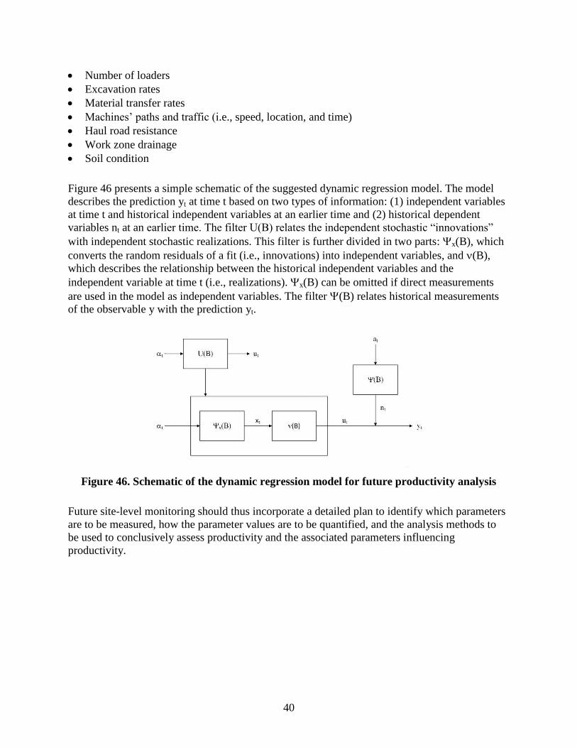
Figure 46 presents a simple schematic of the suggested dynamic regression model. The model
describes the prediction yt at time t based on two types of information: (1) independent variables
at time t and historical independent variables at an earlier time and (2) historical dependent
variables nt at an earlier time. The filter U(B) relates the independent stochastic “innovations”
with independent stochastic realizations. This filter is further divided in two parts: x(B), which
converts the random residuals of a fit (i.e., innovations) into independent variables, and (B),
which describes the relationship between the historical independent variables and the
independent variable at time t (i.e., realizations). x(B) can be omitted if direct measurements
are used in the model as independent variables. The filter (B) relates historical measurements
of the observable y with the prediction yt.
Figure 46. Schematic of the dynamic regression model for future productivity analysis
Future site-level monitoring should thus incorporate a detailed plan to identify which parameters
are to be measured, how the parameter values are to be quantified, and the analysis methods to
be used to conclusively assess productivity and the associated parameters influencing
productivity.
41
REFERENCES
Abdelhamid, T., and Everett, J. (1999). Time Series Analysis for Construction Productivity
Experiments. Journal of Construction Engineering and Management, 125(2), 87-95.
AbouRizk, S., Knowles, P., and Hermann, U. (2001). Estimating Labor Production Rates for
Industrial Construction Activities. Journal of Construction Engineering and
Management, 127(6), 502-511.
Askew, W., Al-Jibouri, S., Mawdesley, M., and Patterson, D. (2002). Planning linear
construction projects: automated method for the generation of earthwork activities.
Automation in Construction, 11(6), 643-653.
Aðalsteinsson, D. H. (2008). GPS machine guidance in construction equipment.
Barlish, K., and Sullivan, K. (2012). How to measure the benefits of BIM — A case study
approach. Automation in Construction, 24, 149-159.
Bender, D. (2010). Implementing building information modeling in the top 100 architecture
firms. Journal of Building Information Modeling, Spring 2010, 23-24.
Bryde, D., Broquetas, M., and Volm, J. M. (2013). The project benefits of Building Information
Modelling (BIM). International Journal of Project Management, 31(7), 971-980.
Cannon, H., and Singh, S. (2000). Models for automated earthmoving. Experimental Robotics
VI, P. I. Corke and J. Trevelyan, eds., Springer-Verlag, London, 163-172.
Capony, A., Lorino, T., Muresan, B., Baudru, Y., Dauvergne, M., Dunand, M., Colin, D., and
Jullien, A. (2012). Assessing the productivity and the environmental impacts of
earthwork machines: a case study for GPS-instrumented excavator. Procedia-Social and
Behavioral Sciences, 48, 256-265.
Chynoweth, P., Christensen, S., McNamara, J., and O'Shea, K. (2007). Legal and contracting
issues in electronic project administration in the construction industry. Structural Survey,
25(3/4), 191-203.
Dawood, N., and Iqbal, N. (2010). Building information modelling (BIM): A visual & whole life
cycle approach. Paper presented at the 10th International Conference on Construction
Applications of Virtual Reality, Sendai, Japan.
Denzer, A., and Hedges, K. (2008). From CAD to BIM: Educational strategies for the coming
paradigm shift. Paper presented at the Architectural Engineering Conference (AEI),
Denver, Colorado.
Eadie, R., Browne, M., Odeyinka, H., McKeown, C., and McNiff, S. (2013). BIM
implementation throughout the UK construction project lifecycle: An analysis.
Automation in Construction, 36, 145-151.
Everett, J. G., and Slocum, A. H. (1994). Automation and robotics opportunities: construction
versus manufacturing. Journal of construction engineering and management, 120(2),
443-452.
Goodrum, P. (2001). The impact of equipment technology on productivity in the United States
construction industry. Doctoral dissertation, University of Texas at Austin.
Hammad, A., Vahdatikhaki, F., Zhang, C., Mawlana, M., and Doriani, A. (2012). Towards the
smart construction site: improving productivity and safety of construction projects using
multi-agent systems, real-time simulation and automated machine control. Proceedings of
the Winter Simulation Conference, 404.
42
Hannon, J. J. (2007). Emerging technologies for construction delivery, NCHRP Synthesis 372,
National Cooperative Highway Resarch Program, Transportation Research Board,
Washington, D.C.
Heravi, G., and Eslamdoost, E. (2015). Applying Artificial Neural Networks for Measuring and
Predicting Construction-Labor Productivity. Journal of Construction Engineering and
Management, 141(10).
Hola, B., and Schabowicz, K. (2010). Estimation of earthworks execution time cost by means of
artificial neural networks. Automation in Construction, 19(5), 570-579.
Huang, X., and Bernold, L. (1997). CAD-integrated excavation and pipe laying. Journal of
Construction Engineering and Management, 123(3), 318-323.
Hwang, S. (2011). Time Series Models for Forecasting Construction Costs Using Time Series
Indexes. Journal of Construction Engineering and Management, 137(9), 656-662.
Jayawardane, A., and Harris, F. (1990). Further development of integer programming in
earthwork optimization. Journal of Construction Engineering and Management, 116(1),
18-34.
Ji, Y., Borrmann, A., Rank, E., Wimmer, J., and Günthner, W. (2009). An Integrated 3D
Simulation Framework for Earthwork Processes. Proceedings of the 26th CIB-W78
Conference on Managing IT in Construction.
Jonasson, S., Dunston, P. S., Ahmed, K., and Hamilton, J. (2002). Factors in productivity and
unit cost for advanced machine guidance. Journal of Construction Engineering and
Management, 128(5), 367-374.
Kamat, V. R., and Martinez, J. C. (2001). Visualizing simulated construction operations in 3D.
Journal of Computing in Civil Engineering, 15(4), 329-337.
Kamat, V. R., and Martinez, J. C. (2003). Validating complex construction simulation models
using 3D visualization. Systems Analysis Modelling Simulation, 43(4), 455-467.
Krishnamurthy, B. K., Tserng, H.-P., Schmitt, R. L., Russell, J. S., Bahia, H. U., and Hanna, A.
S. (1998). AutoPave: towards an automated paving system for asphalt pavement
compaction operations. Automation in Construction, 8(2), 165-180.
Kuo, Y.-c. (2004). Highway earthwork and pavement production rates for construction time
estimation. Doctoral dissertation, University of Texas at Austin.
Liu, D., Cui, B., Liu, Y., and Zhong, D. (2013). Automatic control and real-time monitoring
system for earth–rock dam material truck watering. Automation in Construction, 30, 70-
80.
Miller, S., Hartmann, T., and Dorée, A. (2011). Measuring and visualizing hot mix asphalt
concrete paving operations. Automation in Construction, 20(4), 474-481.
Olatunji, O. A. (2011). A preliminary review on the legal implications of BIM and model
ownership. Journal of Information Technology in Construction, 16, 687-696.
Olearczyk, J., Bouferguène, A., Al-Hussein, M., and Hermann, U. R. (2014). Automating motion
trajectory Of crane-lifted loads. Automation in Construction, 45, 178-186.
Race, S. (2012). BIM demystified, Riba Publishing.
Royston, J. (1982). An extension of Shapiro and Wilk’s W test for normality to large samples.
Applied Statistics, 31, 115-124.
Royston, P. (1995). Remark AS R94: A remark on algorithm AS 181: The W-test for normality.
Applied Statistics, 44, 547-551.
43
Santos, M., Ha, Q., Rye, D., and Durrant-Whyte, H. (2000). Global control of robotic excavation
using fuzzy logic and statecharts. Proceedings of 17th Symposium on Automation and
Robotics in Construction, 595-565.
Sebastian, R. (2010). Breaking through business and legal barriers of open collaborative
processes based on building information modelling (BIM). Proceedings, W113 - Special
Track, 18th CIB World Building Congress, May 2010 Salford, United Kingdom, 166-186.
Stentz, A., Bares, J., Singh, S., and Rowe, P. (1999). A robotic excavator for autonomous truck
loading. Autonomous Robots, 7(2), 175-186.
Steward, B. L., Tang, L., and Han, S. (2015). A Design Framework for Off-road Equipment
Automation. Proceedings of the 2015 Conference on Autonomous and Robotic
Construction of Infrastructure, D. J. White, A. Alhasan, and P. K. Vennapusa, eds., Iowa
State University, Ames, Iowa, 180-196.
Vennapusa, P. K., White, D. J., and Jahren, C. T. (2015). Impacts of Automated Machine
Guidance on Earthwork Operations. Proceedings of the 2015 Conference on Autonomous
and Robotic Construction of Infrastructure, D. J. White, A. Alhasan, and P. K.
Vennapusa, eds., Iowa State University, Ames, Iowa, 207-216.