earthquake ground-motion prediction equations for eastern ... · earthquake ground-motion...
TRANSCRIPT
2181
Bulletin of the Seismological Society of America, Vol. 96, No. 6, pp. 2181–2205, December 2006, doi: 10.1785/0120050245
E
Earthquake Ground-Motion Prediction Equations for Eastern North America
by Gail M. Atkinson and David M. Boore
Abstract New earthquake ground-motion relations for hard-rock and soil sites ineastern North America (ENA), including estimates of their aleatory uncertainty (vari-ability) have been developed based on a stochastic finite-fault model. The modelincorporates new information obtained from ENA seismographic data gathered overthe past 10 years, including three-component broadband data that provide new in-formation on ENA source and path effects. Our new prediction equations are similarto the previous ground-motion prediction equations of Atkinson and Boore (1995),which were based on a stochastic point-source model. The main difference is thathigh-frequency amplitudes (f � 5 Hz) are less than previously predicted (by abouta factor of 1.6 within 100 km), because of a slightly lower average stress parameter(140 bars versus 180 bars) and a steeper near-source attenuation. At frequencies lessthan 5 Hz, the predicted ground motions from the new equations are generally within25% of those predicted by Atkinson and Boore (1995). The prediction equationsagree well with available ENA ground-motion data as evidenced by near-zero averageresiduals (within a factor of 1.2) for all frequencies, and the lack of any significantresidual trends with distance. However, there is a tendency to positive residuals formoderate events at high frequencies in the distance range from 30 to 100 km (by asmuch as a factor of 2). This indicates epistemic uncertainty in the prediction model.The positive residuals for moderate events at �100 km could be eliminated by anincreased stress parameter, at the cost of producing negative residuals in othermagnitude-distance ranges; adjustment factors to the equations are provided that maybe used to model this effect.
Online material: Database of response spectra for hard-rock sites in ENA.
Introduction
A decade has passed since Atkinson and Boore (1995)developed their ground-motion prediction equations for east-ern North America (ENA). The Atkinson and Boore (1995)prediction equations (AB95) were based on a stochasticpoint-source methodology (Boore, 1983), with the model’ssource and attenuation parameters determined from empiri-cal data from small to moderate earthquakes in ENA. Spe-cifically, the AB95 model rested heavily on the two-cornersource spectral model of Atkinson (1993a) and the spectralattenuation model of Atkinson and Mereu (1992).
Since 1995, there have been several advancements thatmake it timely to develop new ENA ground-motion predic-tion equations:
1. An additional 10 years of ground-motion data have beengathered, including broadband data that extend the band-width of ENA ground-motion databases (Atkinson, 2004)and improve the definition of attenuation trends within100 km of the source.
2. New analyses demonstrate that attenuation in ENA in the
first 70 km is faster than previously believed. The geo-metric spreading rate is R�1.3, where R is hypocentraldistance (Atkinson, 2004). The new attenuation has a sig-nificant impact on predicted ground motions.
3. Stochastic finite-fault modeling techniques that can beused to develop regional ground-motion prediction equa-tions for both point sources and large faults have beenextended and validated (Beresnev and Atkinson, 1997a,1998b, 2002; Motazedian and Atkinson, 2005). It hasalso been demonstrated that a point-source model canmimic the salient effects of finite-fault models throughappropriate specification of an equivalent point-sourcerepresentation (Atkinson and Silva, 2000). As a result ofdevelopments in stochastic modeling, it is now feasibleto use a finite-fault model to improve ground-motion pre-dictions for larger earthquakes in ENA. The use of a fi-nite-fault model is particularly important in improvingthe reliability of estimates for large-magnitude events atclose distances, for which the point-source approximationis known to perform poorly.
2182 G. M. Atkinson and D. M. Boore
This article presents new ENA ground-motion predic-tion equations for hard-rock sites based on a stochastic finite-fault model. Relations are also presented for a reference sitecondition of National Earthquake Hazards Reduction Pro-gram (NEHRP) B/C boundary (shear-wave velocity, 760 m/sec), and nonlinear amplification factors are presented thatconvert from B/C boundary to softer site conditions. Theinput parameters to the model are assigned based on currentinformation on ENA source, path, and site effects as obtainedfrom empirical studies of seismographic and strong-motiondata in ENA. The effects of aleatory uncertainty in modelparameters are included in the simulations. Epistemic un-certainty is partially modeled by examining the influence ofepistemic uncertainty in stress parameter, which is the larg-est source of epistemic uncertainty. It is also evaluatedthrough comparisons of the results of this study with otherprediction equations. The stochastic finite-fault model pre-dictions are compared with ENA ground-motion data, andwith other ground-motion prediction equations, includingthe previous point-source predictions of Atkinson and Boore(1995). The model parameters were derived largely fromdata recorded on hard-rock sites (with shear-wave velocity�2 km/sec) in the northeastern United States and south-eastern Canada. However, past studies (Electric Power Re-search Institute [EPRI], 1993) have shown that ground-motion relations are expected to be similar, for a given sitecondition, over a broad region of ENA including the mid-continent.
Methodology and Model Parameters
Ground-motion prediction equations are developed forresponse spectra (pseudo-acceleration, 5% damped), peakground acceleration (PGA) and peak ground velocity (PGV),for hard-rock sites in ENA (near-surface shear-wave velocityb � 2 km/sec, or NEHRP site class A), as a function ofmoment magnitude and closest distance to the fault rupture.For seismic-hazard analysis, we are primarily interested inground motions from earthquakes of moment magnitude(M) �5, at distances less than 100 km from the source.Because of the paucity of recorded ENA ground motions inthis magnitude-distance range, it is not feasible to developENA ground-motion prediction equations directly from re-gression analysis of empirical data. Rather, ENA ground-motion prediction equations are derived from a simulatedground-motion database. The simulated ground motions aredeveloped from a seismological model of source, path, andsite parameters. For this study, the seismological model pa-rameters are obtained using empirical data from small tomoderate ENA earthquakes. The methodology itself has beenvalidated by comparing data and predictions in datarich re-gions. Finally, the model predictions are compared with theavailable ENA ground-motion database and with the predic-tions from other relations.
The simulations to develop the ENA ground-motion pre-diction equations are based on the well-known stochastic
method (Boore, 2003). The stochastic method has been usedto derive ground-motion prediction equations for many dif-ferent regions. Atkinson and Boore (1995) derived ground-motion prediction equations for ENA using a stochasticpoint-source model with an empirical two-corner sourcemodel. Toro et al. (1997) developed similar relations forENA using a Brune single-corner frequency point-sourcemodel. Atkinson and Silva (2000) developed ground-motionprediction equations for California using a stochastic methodthat exploits the equivalence between the finite-fault modeland a two-corner point-source model of the earthquake spec-trum. In each of these cases, region-specific input parametersderived from seismograms were used to specify the modelparameters that drive the ground-motion prediction equa-tions for that region. For California, Atkinson and Silva(2000) showed that the stochastic prediction equations agreewell with empirical regression equations for that region (e.g.,Abrahamson and Silva, 1997; Boore et al., 1997; Sadigh etal., 1997). Stochastic ground-motion prediction equationsprovide a sound basis for estimating peak ground motionsand response spectra for earthquakes of magnitudes 4through 8, at distances from 1 to 200 km over the frequencyrange 0.2 to 20 Hz.
Stochastic Simulation Model
The stochastic model is a widely used tool to simulateacceleration time series and develop ground-motion predic-tion equations (Hanks and McGuire, 1981; Boore, 1983; At-kinson and Boore, 1995, 1997; Toro et al., 1997; Atkinsonand Silva, 2000; Boore, 2003). The stochastic method beginswith the specification of the Fourier spectrum of ground mo-tion as a function of magnitude and distance. The accelera-tion spectrum is typically modeled by a spectrum with anx2 shape, where x � angular frequency (Aki, 1967; Brune,1970, 1971; Boore 1983, 2003). The “x2 model” spectrumis derived for an instantaneous shear dislocation at a point.The acceleration spectrum of the shear wave, A(f), at hy-pocentral distance R from an earthquake is given by:
2 2A( f ) � CM (2p f ) /[1 � ( f / f ) ]0 0
exp(�p fj )exp(�p fR/Qb ) /R (1)0
where M0 is seismic moment and f0 is corner frequency,which is given by f0 � 4.9 * 106 b (Dr/M0)
1/3 where Dr isstress parameter in bars, M0 is in dyne centimeters, and b isshear-wave velocity in kilometers per second (Boore, 1983).The constant C � ℜh�FV /(4pqb3), where ℜh� � radiationpattern (average value of 0.55 for shear waves), F � free-surface amplification (2.0), V � partition onto two horizon-tal components (0.71), q � density, and R � hypocentraldistance (Boore, 1983). The term exp(�pfj0) is a high-cutfilter to account for near-surface attenuation effects, whichdescribe the commonly observed rapid spectral decay at highfrequencies (Anderson and Hough, 1984). In equation (1)the power of R in the denominator of the attenuation term,
Earthquake Ground-Motion Prediction Equations for Eastern North America 2183
exp(�pfR/Qb)/R, is equal to 1, which is appropriate forbody-wave spreading in a whole space. This value can bechanged as needed to account for deviations from 1/R dueto factors such as postcritical reflections from the Moho dis-continuity or multiply reflected waves traveling in the crustalwaveguide. The quality factor, Q(f), is an inverse measureof anelastic attenuation. Through this equation, the spectrumis diminished with distance to account for empirically de-fined attenuation behavior.
Finite-fault modeling has been an important tool for theprediction of ground motion near the epicenters of largeearthquakes (Hartzell, 1978; Irikura, 1983; Joyner andBoore, 1986; Heaton and Hartzell, 1986; Somerville et al.,1991; Tumarkin and Archuleta, 1994; Zeng et al., 1994;Beresnev and Atkinson, 1998a,b). One of the most usefulmethods to simulate ground motion for a large earthquakeis based on the simulation of many small earthquakes assubfaults that constitute an extended fault plane. A largefault is divided into N subfaults and each subfault is consid-ered as a small point source (a method introduced by Hart-zell, 1978). Ground motions of subfaults, each of which maybe calculated by the stochastic point-source method as de-scribed previously, are summed with a proper time delay inthe time domain to obtain the ground motion from the entirefault, a(t):
nl nw
a(t) � a (t � Dt ), (2)� � ij iji�1 j�1
where nl and nw are the number of subfaults along the lengthand width of main fault, respectively (nl * nw � N), andDtij is the relative time delay for the radiated wave from theijth subfault to reach the observation point. The aij (t) areeach calculated by the stochastic point-source method(Boore, 1983, 2003).
In this study, we use a stochastic finite-fault approach,allowing us to incorporate significant finite-fault effects suchas the geometry of larger ruptures and its effects on attenu-ation, and directivity. The simulations are performed withthe computer code EXSIM (Extended Finite-Fault Simula-tion; Motazedian and Atkinson, 2005). This code is an up-dated version of the well-known FINSIM stochastic finite-fault model code (Beresnev and Atkinson, 1997a, 1998b,2002). The modifications to FINSIM introduce the new con-cept of a “dynamic corner frequency,” which decreases withtime as the rupture progresses, to model more closely theeffects of finite-fault geometry on the frequency content ofradiated ground motions (Motazedian and Atkinson, 2005).The model has several significant advantages over previousstochastic finite-fault models, including independence of re-sults from subfault size, conservation of radiated energy, andthe ability to have only a portion of the fault active at anytime during the rupture (simulating self-healing behavior[Heaton, 1990]).
EXSIM model parameters that represent the earthquakesource processes have been calibrated for general applica-
tions, using data from 27 moderate to large well-recordedearthquakes in California (Motazedian and Atkinson, 2005).For use in ENA, the model requires region-specific source,attenuation, and generic site parameters, which are derivedfrom recordings of small to moderate earthquakes.
We use EXSIM to simulate a ground-motion databasefrom which to develop ground-motion equations. This ap-proach is taken because there are not enough real data in themagnitude-distance ranges of engineering interest (M 5 to7.5 at distances less than 200 km) to derive purely empiri-cally based ground-motion prediction equations. We use theempirical data to establish the underlying parameters andvalidate the model predictions. The region-specific param-eters needed for simulations are:
1. Attenuation of Fourier amplitudes with distance (appar-ent geometric spreading and Q-value)
2. Duration of ground motion as a function of magnitudeand distance
3. Regional generic crust/site amplifications and physicalconstants
4. Source parameters for simulation: stress parameter andpulsing percentage. The stress parameter is most impor-tant because it controls the amplitudes of high-frequencyradiation. The percentage of the fault that is pulsing atany time (simulating healing behavior as the rupture frontpasses) has an influence on the relative amount of low-frequency radiation. Simulated ground motions are sen-sitive to the stress parameter, but there is limited sensi-tivity to pulsing percentage. Thus stress is the key sourceparameter to be established. The stress parameter de-scribes the level of the acceleration spectrum near thesource, and is equivalent to the Brune model stress pa-rameter as described by Boore (1983) and Atkinson andBoore (1995).
With these parameters established, we can use the cal-ibrated EXSIM model to extend our predictions to the mag-nitude-distance range of interest. We then compare predic-tions with ENA data.
Model Parameters for Simulationsand Their Uncertainty
The input model parameters for ENA ground-motionsimulations are discussed next. For parameters with signifi-cant variability, we consider the effects of aleatory uncer-tainty, expressing random variability in the parameter fromone ground-motion realization to another (Toro and Mc-Guire, 1987). We do not attempt to model the effects ofepistemic uncertainty (uncertainty in the correct medianvalue of each parameter) in a comprehensive way in oursimulations, because we do not believe this would be anappropriate way to deal with the broader issue of epistemicuncertainty in ground-motion prediction equations. To prop-erly consider epistemic uncertainty, one needs to consider awide variety of alternative models and theories of ground
2184 G. M. Atkinson and D. M. Boore
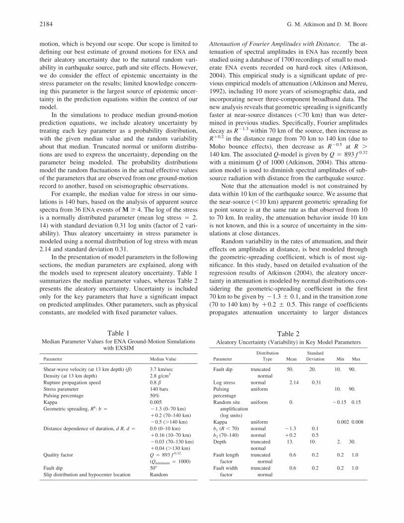
Table 1Median Parameter Values for ENA Ground-Motion Simulations
with EXSIM
Parameter Median Value
Shear-wave velocity (at 13 km depth) (b) 3.7 km/secDensity (at 13 km depth) 2.8 g/cm3
Rupture propagation speed 0.8 b
Stress parameter 140 barsPulsing percentage 50%Kappa 0.005Geometric spreading, Rb: b � �1.3 (0–70 km)
�0.2 (70–140 km)�0.5 (�140 km)
Distance dependence of duration, d R, d � 0.0 (0–10 km)�0.16 (10–70 km)�0.03 (70–130 km)�0.04 (�130 km)
Quality factor Q � 893 f 0.32
(Qminimum � 1000)Fault dip 50�Slip distribution and hypocenter location Random
motion, which is beyond our scope. Our scope is limited todefining our best estimate of ground motions for ENA andtheir aleatory uncertainty due to the natural random vari-ability in earthquake source, path and site effects. However,we do consider the effect of epistemic uncertainty in thestress parameter on the results; limited knowledge concern-ing this parameter is the largest source of epistemic uncer-tainty in the prediction equations within the context of ourmodel.
In the simulations to produce median ground-motionprediction equations, we include aleatory uncertainty bytreating each key parameter as a probability distribution,with the given median value and the random variabilityabout that median. Truncated normal or uniform distribu-tions are used to express the uncertainty, depending on theparameter being modeled. The probability distributionsmodel the random fluctuations in the actual effective valuesof the parameters that are observed from one ground-motionrecord to another, based on seismographic observations.
For example, the median value for stress in our simu-lations is 140 bars, based on the analysis of apparent sourcespectra from 36 ENA events of M � 4. The log of the stressis a normally distributed parameter (mean log stress � 2.14) with standard deviation 0.31 log units (factor of 2 vari-ability). Thus aleatory uncertainty in stress parameter ismodeled using a normal distribution of log stress with mean2.14 and standard deviation 0.31.
In the presentation of model parameters in the followingsections, the median parameters are explained, along withthe models used to represent aleatory uncertainty. Table 1summarizes the median parameter values, whereas Table 2presents the aleatory uncertainty. Uncertainty is includedonly for the key parameters that have a significant impacton predicted amplitudes. Other parameters, such as physicalconstants, are modeled with fixed parameter values.
Attenuation of Fourier Amplitudes with Distance. The at-tenuation of spectral amplitudes in ENA has recently beenstudied using a database of 1700 recordings of small to mod-erate ENA events recorded on hard-rock sites (Atkinson,2004). This empirical study is a significant update of pre-vious empirical models of attenuation (Atkinson and Mereu,1992), including 10 more years of seismographic data, andincorporating newer three-component broadband data. Thenew analysis reveals that geometric spreading is significantlyfaster at near-source distances (�70 km) than was deter-mined in previous studies. Specifically, Fourier amplitudesdecay as R�1.3 within 70 km of the source, then increase asR�0.2 in the distance range from 70 km to 140 km (due toMoho bounce effects), then decrease as R�0.5 at R �140 km. The associated Q-model is given by Q � 893 f 0.32
with a minimum Q of 1000 (Atkinson, 2004). This attenu-ation model is used to diminish spectral amplitudes of sub-source radiation with distance from the earthquake source.
Note that the attenuation model is not constrained bydata within 10 km of the earthquake source. We assume thatthe near-source (�10 km) apparent geometric spreading fora point source is at the same rate as that observed from 10to 70 km. In reality, the attenuation behavior inside 10 kmis not known, and this is a source of uncertainty in the sim-ulations at close distances.
Random variability in the rates of attenuation, and theireffects on amplitudes at distance, is best modeled throughthe geometric-spreading coefficient, which is of most sig-nificance. In this study, based on detailed evaluation of theregression results of Atkinson (2004), the aleatory uncer-tainty in attenuation is modeled by normal distributions con-sidering the geometric-spreading coefficient in the first70 km to be given by �1.3 � 0.1, and in the transition zone(70 to 140 km) by �0.2 � 0.5. This range of coefficientspropagates attenuation uncertainty to larger distances
Table 2Aleatory Uncertainty (Variability) in Key Model Parameters
ParameterDistribution
Type MeanStandardDeviation Min Max
Fault dip truncatednormal
50. 20. 10. 90.
Log stress normal 2.14 0.31Pulsingpercentage
uniform 10. 90.
Random siteamplification(log units)
uniform 0. �0.15 0.15
Kappa uniform 0.002 0.008b1 (R � 70) normal �1.3 0.1b2 (70–140) normal �0.2 0.5Depth truncated
normal13. 10. 2. 30.
Fault lengthfactor
truncatednormal
0.6 0.2 0.2 1.0
Fault widthfactor
truncatednormal
0.6 0.2 0.2 1.0
Earthquake Ground-Motion Prediction Equations for Eastern North America 2185
(�140 km) and is sufficient to model the net effects of un-certainty in all attenuation parameters. Note that attenuationuncertainties are coupled, such that uncertainties in geomet-ric spreading and Q should not actually be treated as inde-pendent; mapping all of the attenuation uncertainty into geo-metric spreading is a simple way to approximate theexpected overall behavior. We have not attempted to modelthe uncertainty in a detailed way, merely to mimic the be-havior that is observed in ENA databases.
Atkinson (2004) found that the attenuation in ENA de-pends slightly on the focal depth of the earthquake, and pro-posed depth-correction factors to the attenuation modelbased on depth. These factors were not included in the sim-ulations, because the attenuation rates are being randomizedto account for their aleatory uncertainty, and the depth-correction factors to the attenuation are a relatively insignif-icant component of the overall attenuation; thus, depth ef-fects on attenuation are considered part of the overallattenuation uncertainty modeled through the assumed vari-ability in geometric-spreading rates.
Duration of Ground Motion. The duration (T) of an earth-quake signal at hypocentral distance R can generally be rep-resented as (Atkinson and Boore, 1995):
T (R) � T � dR, (3)0
where T0 is the source duration, and d is the coefficient con-trolling the increase of duration with distance; d is derivedempirically. d may be a single coefficient describing all dis-tances of interest (e.g., Atkinson, 1993b), or it can take dif-ferent values depending on the distance range (e.g., Atkinsonand Boore, 1995). The empirical duration model of Atkinsonand Boore (1995) was adopted for this study. The durationincreases in a hinged quadlinear fashion from the source,mimicking the form of the attenuation model. The coeffi-cients for d are 0.0, 0.16, �0.03, and 0.04, for the distanceranges 0 to 10 km, 10 to 70 km, 70 to 130 km, and �130 km,respectively (see Atkinson and Boore, 1995). In Atkinsonand Boore (1995), the zero distance duration was 0.0 sec;here we let it be 1.0 sec. The source duration is estimated asthe subfault rise time, as determined by the subfault radiusand the rupture-propagation speed. We re-examined this du-ration model in light of recent data, and saw no evidencethat this model should be revised. The uncertainty in dura-tion is not modeled, as it is less significant than uncertaintyin other parameters in terms of its impact on simulatedground-motion amplitudes.
Regional Generic Crust/Site Amplifications and PhysicalConstants. The shear-wave velocity (b) at average focaldepths (near 13 km) is assumed to be 3.7 km/sec, with den-sity (q) 2.8 g/cm3. These are typical regional values (Booreand Joyner, 1997). Shear-wave velocity actually depends ondepth, so in the modeling of alternative focal depths (dis-cussed in a following section), the value of b is selected
based on the event depth, such that b increases from a valueof 3.1 km/sec at a depth of 5 km, through the value of3.7 km/sec at 13 km, to a maximum of 3.8 km/sec for depthsof 14.5 km or more. These values were based on typicalcrustal shear-wave velocity profiles (e.g., Somerville et al.,2001). The physical constants are not a significant source ofuncertainty.
Amplification of horizontal-component ground mo-tions, for rock sites, occurs because of the combined effectsof the velocity gradient in the crust and near-surface ampli-fication due to the weathered layer of rock in the top fewmeters. (There is additional site response for soil sites, butthis is not considered within the simulations; modificationsto model soil sites by applying additional soil amplificationsare discussed later.) An approximation of the amount of am-plification for rock sites may be obtained empirically usingthe horizontal-to-vertical component ratios (H/V ratios) forrock sites in ENA, as discussed by Atkinson (2004). Thebasic idea is that amplification of the vertical component isvery small compared with that of the horizontal component,allowing H/V to provide a first-order site-amplification es-timate. A criticism of the H/V technique, as originally ap-plied to microtremor measurements (e.g., Nakamura’s tech-nique), is that it is largely a measure of Rayleigh waveellipticity. However, it has been pointed out that when ap-plied to body waves, as measured from earthquakes, theH/V ratio may be largely controlled by site response (Lermoand Chavez-Garcia, 1993). Several studies support the hy-pothesis of Lermo and Chavez-Garcia (1993) that the ob-served H/V ratios are a measure of the amplification of seis-mic ground motions due to their transit through the crustaland/or near-surface velocity gradient. For example, Atkin-son and Cassidy (2000) show that the H/V ratio for rock sitesin western British Columbia matches the amplification thatwould be expected based on the regional shear-wave veloc-ity gradient. The expected amplification was calculated fromthe regional shear-wave velocity profile, using the quarter-wavelength approximation (Boore and Joyner, 1997) to es-timate the amplification as a function of frequency. Atkinsonand Cassidy (2000) also studied ground motions for soft soilsites in the Fraser Delta, British Columbia, that amplify weak
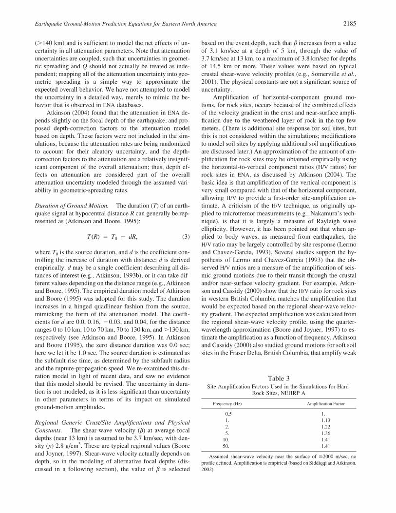
Table 3Site Amplification Factors Used in the Simulations for Hard-
Rock Sites, NEHRP A
Frequency (Hz) Amplification Factor
0.5 1.1. 1.132. 1.225. 1.36
10. 1.4150. 1.41
Assumed shear-wave velocity near the surface of �2000 m/sec, noprofile defined. Amplification is empirical (based on Siddiqqi and Atkinson,2002).
2186 G. M. Atkinson and D. M. Boore
motions three to five times in the frequency range from 0.3to 4 Hz, and concluded that observed amplifications wereconsistent with the H/V ratios. Siddiqqi and Atkinson (2002)report a similar finding for rock sites in different environ-ments across Canada, including eastern Canada.
The assumed amplification for ENA rock sites increasesfrom a value of 1.0 for frequencies less than 0.5 Hz, to avalue of 1.41 at f � 10 Hz, as given by Siddiqqi and Atkin-son (2002). Table 3 provides the amplification factors usedfor the hard-rock site simulations (NEHRP A); Table 4 pro-vides those that apply for NEHRP B/C boundary site condi-tions (discussed later in the text). The high-frequency am-plification factor for hard rock (�1.4) is consistent withnear-surface shear-wave velocities of about 2 km/sec, ac-cording to simple calculations with the quarter-wavelengthimpedance-based method of Boore and Joyner (1997) (e.g.,
). These inferred near-surface velocities for3.7/1.9 � 1.4�hard-rock sites in ENA are consistent with estimates basedon shear-wave refraction studies (Beresnev and Atkinson,1997b).
Variability in site amplification is modeled by using anadditional amplification factor randomly drawn from a uni-form distribution ranging from �0.15 to �0.15 log unitsfor each trial. In the aleatory sense, this uncertainty repre-sents the typical random variability that is seen even amongnearby sites with apparently similar site conditions (Boore,2004).
Amplification effects are counteracted at high frequen-cies by the effects of the high-frequency shape factor j0
(Anderson and Hough, 1984). j0 acts to diminish spectralamplitudes rapidly at high frequencies, and is believed to beprimarily a site effect. For hard-rock sites in ENA, the effectsof j0 are nearly negligible. Atkinson (1996) estimated a j0
value of 0.002. In this study, a careful examination of thespectral data presented by Atkinson (2004) was made tosearch for the values of j0 to use in the simulations. This
indicated a minimum j0 of 0, with a maximum value forindividual records of 0.01. The aleatory uncertainty in j0 isrepresented by a uniform distribution from 0.002 to 0.008.As discussed later, the simulation results are not sensitive tothe kappa parameter, except for response spectra at frequen-cies � 20 Hz.
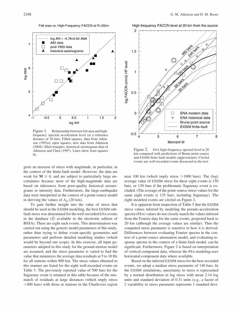
Source Parameters for Simulation. The most importantsource parameter for the simulations is the stress parameter,which controls the spectral amplitudes at high frequencies.The distribution of this parameter was determined from thehigh-frequency level of apparent source spectra for all ENAevents of M � 4, as listed in Table 5, at a reference distanceof 20 km (denoted Ahf (20 km)). The source spectra for in-strumentally recorded earthquakes were determined by usingthe attenuation model of Atkinson (2004) to correct allvertical-component observations on rock back to the refer-ence distance of 20 km; the vertical component data on rockare used as they are relatively free from site-amplificationeffects. Note that this attenuation correction assumes a pointsource, which will be adequate for most of the instrumentalevents because of their small to moderate size. The sourcespectrum of an event was obtained by averaging the logamplitudes at this reference distance over all stations thatrecorded the event. The stress was then defined as the Brunestress value associated with this high-frequency spectrallevel; this value was determined using equation (1), with theparameter values adopted in this study. This stress value alsoassumes a point source (Brune model). The frequency rangeused to determine the high-frequency level was 5 to 10 Hzfor the events with modern instrumental data. For early-instrumental data from large ENA events (Atkinson andChen, 1997), the maximum available frequencies are in therange from 1.5 to 2 Hz; for these events this frequency rangewas used to define Ahf , under the assumption that earth-quakes of M �6 will have corner frequencies less than 1 Hz.High-frequency spectral levels were also estimated for pre-instrumental events based on their felt area. As shown byAtkinson (1993a), the felt area of an earthquake is well cor-related with high-frequency spectral level. The empirical re-lationship of Atkinson (1993a) between these two parame-ters was updated in this study to include all events through2003 with both determined spectral levels and felt areas. Thenew relationship for Ahf (20 km) based on felt area is shownin Figure 1 and given by:
log A (20 km) � �4.78 � 0.92 log A (4)hf felt
where Ahf (20 km) is in centimeters per second and Afelt isin kilometers squared. This relationship was used in Table 5to determine the point-source stress parameter for eventshaving no modern instrumental data, but a well-determinedfelt area. In preparing Table 5, only events with a knownmoment magnitude (from independent studies) were consid-ered, except for the 1811 New Madrid and 1886 Charlestonevents, which were assigned nominal moment magnitudes
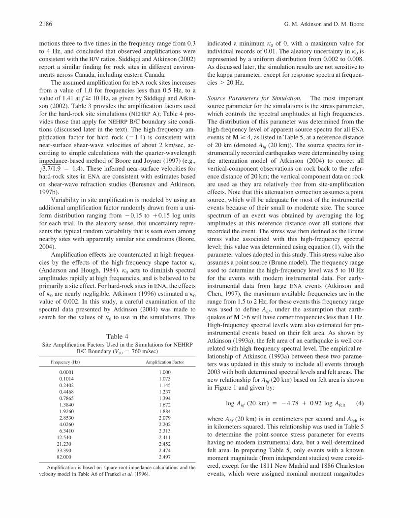
Table 4Site Amplification Factors Used in the Simulations for NEHRP
B/C Boundary (V30 � 760 m/sec)
Frequency (Hz) Amplification Factor
0.0001 1.0000.1014 1.0730.2402 1.1450.4468 1.2370.7865 1.3941.3840 1.6721.9260 1.8842.8530 2.0794.0260 2.2026.3410 2.313
12.540 2.41121.230 2.45233.390 2.47482.000 2.497
Amplification is based on square-root-impedance calculations and thevelocity model in Table A6 of Frankel et al. (1996).
Earthquake Ground-Motion Prediction Equations for Eastern North America 2187
of 7.5 and 7.0, respectively (see Johnston, 1996; Hough etal., 2000).
On Figure 2, the high-frequency spectral levels for ENAevents (from Table 5) are plotted versus M, along with thepredicted behavior for both Brune point-source and EXSIMfinite-fault models. The Brune model predictions are precise,as they are analytically specified (equation 1), whereas theEXSIM values are not. The EXSIM values were obtained byperforming trial simulations with different input values ofstress, for fault distances of approximately 20 km, and ob-taining average Fourier accelerations in this distance range.They are intended to show overall trends only. Note that theEXSIM predictions appear very similar to the Brune point-source predictions for a given stress at magnitudes less than
6. At larger magnitudes, the EXSIM model predicts lowernear-source motions than the point source due to finite-faulteffects; this is because much of the extended fault plan is faraway from the observation point. This trend is believed tobe responsible for the conclusion of some studies that, whenusing a point-source model, a decreasing trend in stress withincreasing magnitude is obtained (e.g., as discussed in At-kinson and Silva, 2000).
Overall, we conclude from Figure 2 that there is noevidence of a decreasing trend of stress with increasing mag-nitude. Furthermore, the determination of a stress parameternear 200 bars for the 2001 M 7.7 Bhuj, India earthquake(Singh et al., 2004) argues against a decreasing stress trendfor large intracontinental events. If anything, Figure 2 sug-
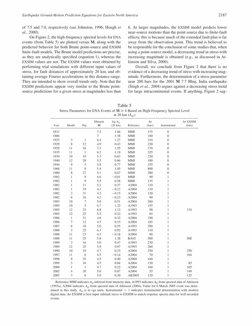
Table 5Stress Parameters for ENA Events of M � 4 Based on High-Frequency Spectral Level
at 20 km (Ahf )
Year Month DayMoment
Mlog Ahf
(20 km) ReferenceDr
(bars) InstrumentalDr EXSIM
(bars)
1811 7.5 1.66 MMI 175 01886 7 1.38 MMI 160 01925 3 1 6.4 1.27 MMI 310 01929 8 12 4.9 0.43 MMI 230 01929 11 18 7.3 1.55 MMI 170 01935 11 1 6.2 1.19 MMI 325 01939 10 19 5.3 0.63 MMI 230 01940 12 20 5.5 0.66 MMI 180 01944 9 5 5.8 0.77 MMI 155 01968 11 9 5.4 1.05 MMI 800 01980 8 27 5.1 0.67 MMI 380 01982 1 9 4.6 �0.01 MMI 90 11982 1 9 5.5 0.58 MMI 135 11982 1 11 5.2 0.37 A2004 110 11982 1 19 4.3 �0.13 A2004 110 11982 3 31 4.2 �0.15 A2004 120 11982 6 16 4.2 �0.23 A2004 90 11983 10 7 5.0 0.51 A2004 260 11985 10 5 6.7 1.22 A1993 155 11985 12 23 6.8 1.12 A1993 90 1 1341985 12 25 5.2 0.22 A1993 65 11986 1 31 4.8 0.32 A2004 190 11986 7 12 4.5 0.15 A2004 185 11987 6 10 5.0 0.55 A1993 290 11988 3 25 6.3 0.92 A1993 110 11988 11 23 4.3 �0.18 A2004 90 11988 11 25 5.8 1.28 BA92 500 1 5001989 3 16 5.0 0.47 A1993 230 11989 12 25 5.9 0.97 A1993 260 11990 10 19 4.7 0.33 A2004 250 1 2501997 11 6 4.5 �0.14 A2004 70 1 1041998 9 25 4.5 0.40 A2004 440 11999 3 16 4.5 0.04 A2004 130 1 852000 1 1 4.7 0.22 A2004 160 1 1052002 4 20 5.0 0.07 A2004 55 1 1492005 3 6 5.0 0.30 AB2005 120 1 125
Reference MMI indicates Ahf inferred from intensity data, A1993 indicates Ahf from spectral data of Atkinson(1993a), A2004 indicates Ahf from spectral data of Atkinson (2004). Value for 6 March 2005 event was deter-mined in this study. Ahf is in cgs units. Instrumental � 1 indicates instrumental determination with moderndigital data. Dr EXSIM is best input subfault stress to EXSIM to match response spectra data for well-recordedevents.
2188 G. M. Atkinson and D. M. Boore
gests an increase of stress with magnitude, in particular, inthe context of the finite-fault model. However, the data areweak for M � 6, and are subject to particularly large un-certainties because most of the high-magnitude data arebased on inferences from poor-quality historical seismo-grams or intensity data. Furthermore, the large-earthquakedata were interpreted in the context of a point-source modelin deriving the values of Ahf (20 km).
To gain further insight into the value of stress thatshould be used in the EXSIM modeling, the best EXSIM sub-fault stress was determined for the well-recorded ENA eventsin the database ( E available in the electronic edition ofBSSA). There are eight such events. This determination wascarried out using the generic model parameters of this study,rather than trying to define event-specific geometries andparameters and perform detailed modeling studies (whichwould be beyond our scope). In this exercise, all input pa-rameters adopted in this study for the ground-motion modelare assumed, and the stress parameter is varied to find thevalue that minimizes the average data residuals at 5 to 10 Hzfor all stations within 800 km. The stress values obtained inthis manner are listed for the eight well-recorded events onTable 5. The previously reported value of 500 bars for theSaguenay event is retained in this table because of the mis-match of residuals at large distances (which imply stress�400 bars) with those at stations in the Charlevoix region
near 100 km (which imply stress �1000 bars). The (log)average value of EXSIM stress for these eight events is 150bars, or 130 bars if the problematic Saguenay event is ex-cluded. (The average of the point-source stress values for thesame eight events is 135 bars, including Saguenay). Theeight modeled events are circled on Figure 2.
It is apparent from inspection of Table 5 that the EXSIMstress values inferred by modeling the pseudo-accelerationspectra (PSA) values do not closely match the values inferredfrom the Fourier data for the same events, projected back to20 km (although the average values are similar). Thus thecomputed stress parameter is sensitive to how it is derived.Differences between evaluating Fourier spectra in the con-text of a point-source attenuation model, and evaluating re-sponse spectra in the context of a finite-fault model, can besignificant. Furthermore, Figure 2 is based on interpretationof vertical-component data, whereas the PSA modeling useshorizontal-component data where available.
Based on the inferred EXSIM stress for the best-recordedevents, we adopt a median stress parameter of 140 bars. Inthe EXSIM simulations, uncertainty in stress is representedby a normal distribution in log stress with mean 2.14 logunits and standard deviation of 0.31 units (e.g., a factor of2 variability in stress parameter represents 1 standard devi-
Figure 1. Relationship between felt area and high-frequency spectral acceleration level (at a referencedistance of 20 km). Filled squares, data from Atkin-son (1993a); open squares, new data from Atkinson(2004); filled triangles, historical seismogram data ofAtkinson and Chen (1997). Lines show least-squaresfit.
Figure 2. ENA high-frequency spectral level at 20km compared with predictions of Brune point-sourceand EXSIM finite-fault models (approximate). Circledevents are well-recorded events discussed in the text.
Earthquake Ground-Motion Prediction Equations for Eastern North America 2189
ation). Other interpretations of the data in Table 5 are pos-sible, leading to other alternative values for the stress param-eter. We provide a mechanism for adjusting the equations tomodel a higher- or lower-stress parameter; these adjustmentsmay be useful in the interpretation of specific events, or inmodeling epistemic uncertainty in predictions due to uncer-tainty in the median stress parameter.
Another issue that arises in assigning the stress-param-eter distribution is an apparent difference in the medianstress for the instrumental data and that inferred from thehistorical data, as can be seen on Figure 2. This could beinterpreted in the context of an increasing trend of stressparameter with magnitude, because of the relative distribu-tion of the data sources in magnitude (historical data domi-nate the large-magnitude data). Due to the large uncertaintiesin the historical data as mentioned previously, we do notconsider the apparent differences in stress compelling. Fur-thermore, finite-fault modeling of data in regions such asCalifornia, which have better data coverage at higher mag-nitudes, favor constant-stress or decreasing-stress scalingwith increasing magnitude (Atkinson and Silva, 1997,2000). Therefore, we retain a constant-stress-scaling modelfor the predictions. Description of the source properties re-mains our biggest source of uncertainty in modeling ENAground motions, and the area that most needs improvementin the future.
The percentage-pulsing area describes how much of thefault plane in slipping at any moment in time. This parameteris assumed based on calibration studies with California data(Motazedian and Atkinson, 2005). It is assigned a relativelylarge aleatory variability, represented by a uniform distri-bution from 10% to 90%. This parameter is not well deter-mined, but does not exert a significant influence on the sim-ulated amplitudes at most frequencies (it exerts someinfluence at lower frequencies, as discussed by Motazedianand Atkinson, 2005).
Earthquake focal depths in ENA cover a broad rangefrom a few kilometers to 30 km. Recent depth determina-tions (Ma and Atkinson, 2006) were used to determine amean focal depth of 13 km. Depth is assumed to be trun-cated-normally distributed, with a standard deviation of10 km. The normal distribution is truncated to provide aminimum depth of 2 km, and maximum depth of 30 km.This depth is used to fix the center of the fault plane for thesimulations, in the vertical dimension. Once the location ofthe fault plane within the crust is fixed, the subfault at whichthe rupture is assumed to initiate is drawn randomly.
The geometry of the fault plane and its placement withinthe crust is treated as follows. The fault dip is assumed tobe a normally distributed random variable with a value of50 � 20 degrees. The fault length and width, which arefunctions of magnitude, are also considered uncertain.EXSIM assumes the fault lengths and widths given by theglobal empirical relationships of Wells and Coppersmith(1994). However, recent data suggest that ENA fault dimen-sions are probably significantly smaller for a given moment
magnitude (Somerville et al., 2001). This effect is modeledby multiplying the fault length and width obtained by theWells and Coppersmith relations by a normally distributedfactor, taken as 0.6 � 0.2 for both length and width; thedistributions are truncated to stipulate a minimum factor of0.2 and maximum factor of 1.0. The net effect of these fac-tors is to assign a fault area that is on average about onethird the equivalent fault area for events in active tectonicregions. These factors do not have a significant impact onpredicted amplitudes, except for very large events (M �7).Just for the geometric purposes of placing the fault withinthe crust, it is assumed that the depth of the hypocenter cor-responds to the middle of the fault width; if this implies asurface rupture, the fault width extends from the surface tothe depth indicated by the fault width and dip. When gen-erating the ground motions, the actual location of the hy-pocenter on the fault plane is assumed to be random, as isthe slip distribution. (Thus the actual depth of the hypocenterwill not match the focal depth used to define the midpointof the fault for an individual simulation, but will match inan average sense over many simulations.)
Results
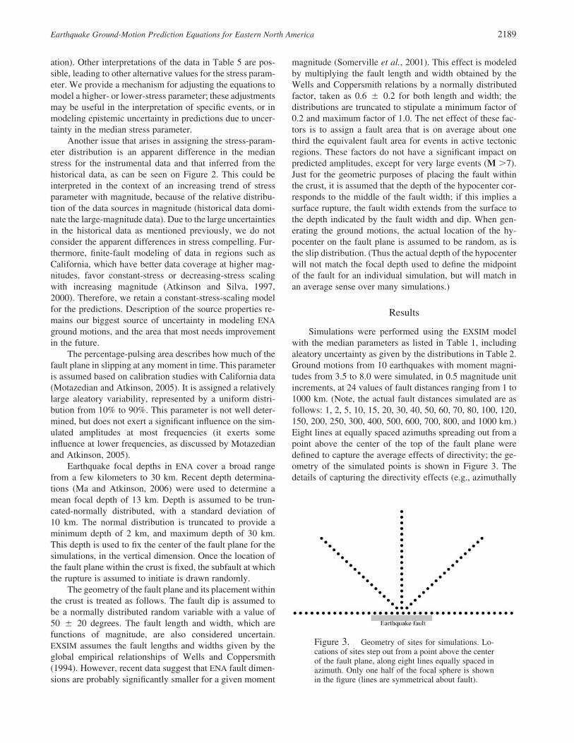
Simulations were performed using the EXSIM modelwith the median parameters as listed in Table 1, includingaleatory uncertainty as given by the distributions in Table 2.Ground motions from 10 earthquakes with moment magni-tudes from 3.5 to 8.0 were simulated, in 0.5 magnitude unitincrements, at 24 values of fault distances ranging from 1 to1000 km. (Note, the actual fault distances simulated are asfollows: 1, 2, 5, 10, 15, 20, 30, 40, 50, 60, 70, 80, 100, 120,150, 200, 250, 300, 400, 500, 600, 700, 800, and 1000 km.)Eight lines at equally spaced azimuths spreading out from apoint above the center of the top of the fault plane weredefined to capture the average effects of directivity; the ge-ometry of the simulated points is shown in Figure 3. Thedetails of capturing the directivity effects (e.g., azimuthally
Figure 3. Geometry of sites for simulations. Lo-cations of sites step out from a point above the centerof the fault plane, along eight lines equally spaced inazimuth. Only one half of the focal sphere is shownin the figure (lines are symmetrical about fault).
2190 G. M. Atkinson and D. M. Boore
determined lines or a “racetrack” of points at fixed distance)are relatively unimportant because of the numerous distancesand magnitudes simulated, which effectively act to random-ize the geometry. Tests were performed to confirm that theresults are unchanged if the number of simulated azimuthsis doubled or quadrupled. For each magnitude and obser-vation point, 20 random trials were performed. Thus a total
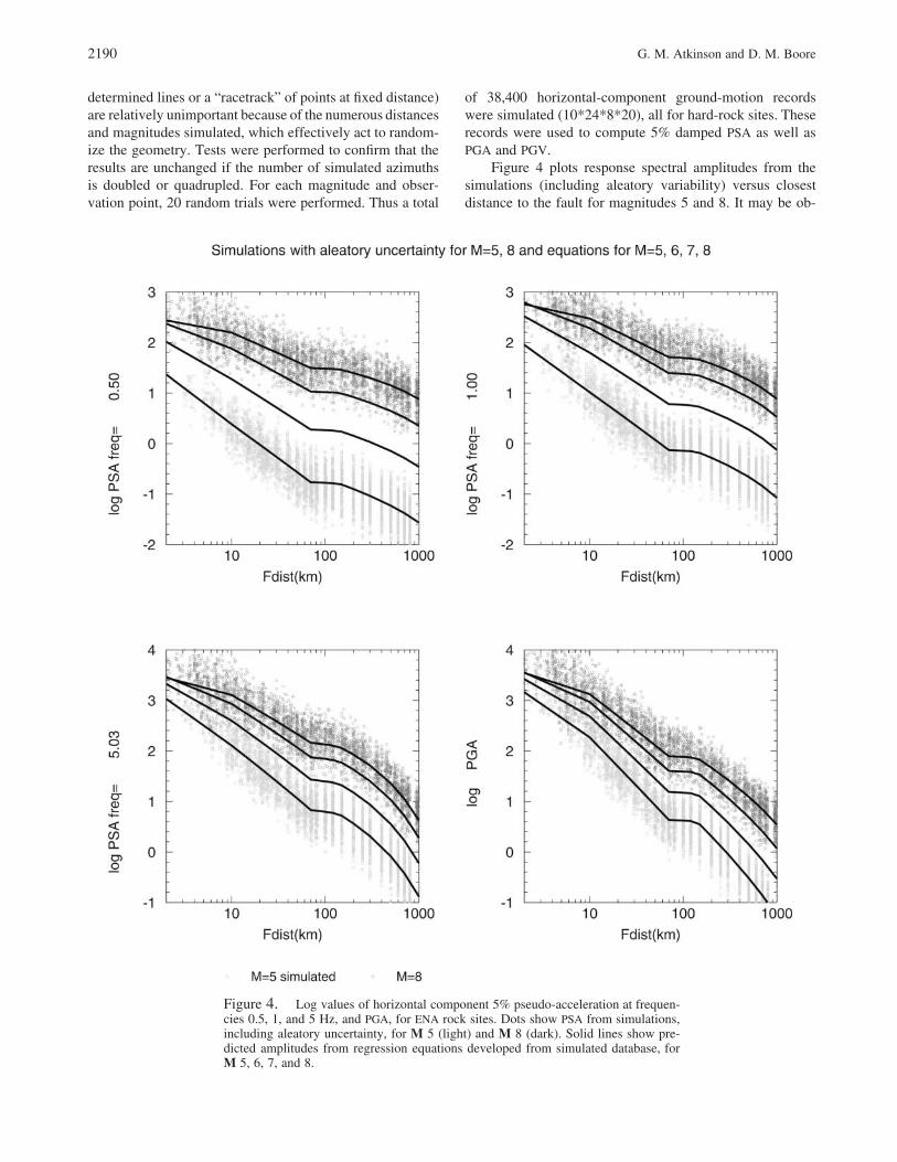
of 38,400 horizontal-component ground-motion recordswere simulated (10*24*8*20), all for hard-rock sites. Theserecords were used to compute 5% damped PSA as well asPGA and PGV.
Figure 4 plots response spectral amplitudes from thesimulations (including aleatory variability) versus closestdistance to the fault for magnitudes 5 and 8. It may be ob-
Figure 4. Log values of horizontal component 5% pseudo-acceleration at frequen-cies 0.5, 1, and 5 Hz, and PGA, for ENA rock sites. Dots show PSA from simulations,including aleatory uncertainty, for M 5 (light) and M 8 (dark). Solid lines show pre-dicted amplitudes from regression equations developed from simulated database, forM 5, 6, 7, and 8.
Earthquake Ground-Motion Prediction Equations for Eastern North America 2191
served that the highest simulated amplitudes have been trun-cated in the y scale chosen for the plots. The highest spectralamplitudes, as well as the highest simulated PGA, reach 4.6log units for a few of the most extreme points (M 8 at 1km). We make no claims that such amplitudes are physicallypossible—they are merely the result of the simulation ex-ercise, which does not account for factors that may act tolimit extreme amplitudes. The figure also plots curves thatrepresent the median amplitudes for M 5, 6, 7, and 8. Themedian values for near-source amplitudes from large events(3.5 log units at high frequencies and PGA) appear reason-able for a very hard rock-site condition. The curves weredetermined by a standard regression analysis to an equationin moment magnitude (M) and closest distance to the fault(Rcd) of the form:
2Log PSA � c � c M � c M � (c � c M) f1 2 3 4 5 1
� (c � c M) f � (c � c M) f (5)6 7 2 8 9 0
� c R � S,10 cd
where f0 � max(log(R0/Rcd), 0); f1 � min(log Rcd, log R1);f2 � max (log (Rcd/R2), 0); R0 � 10; R1 � 70; R2 � 140;and S � 0 for hard-rock sites; its value for soil sites isdiscussed in the next section and given in equation (7a),(7b).Note that this form assumes linearity of motions for hard-rock sites, but can accommodate nonlinearity for soil sites(equation 7a,7b).
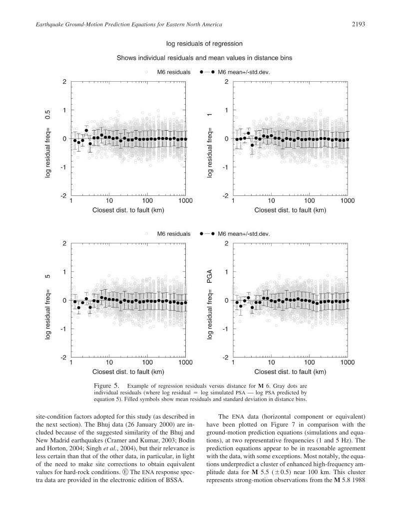
The coefficients of the equation are given in Table 6.The equations do an excellent job of reproducing the simu-lations; there are no significant residual trends with distanceor magnitude, as shown for an example magnitude (M 6) onFigure 5. The aleatory uncertainty is independent of mag-nitude and distance, with an average value of 0.30 log unitsfor all frequencies. This calculated variability, based purelyon the simulation parameters, is slightly larger than typicallyobserved values for empirical strong ground motion predic-tion equations in California (e.g., Boore et al., 1997; Abra-hamson and Silva, 1997). The amount of variability in thesimulations is consistent with that observed in the ENA data,and may reflect the apparently large variability in ENA stressparameters. On the other hand, one could argue that the vari-ability of ground motions should be the same in ENA as itis in California, in which case the simulated variability mayslightly overestimate the actual variability. Note, though,that recent estimates of variability of ground motions foractive tectonic regions (Boore and Atkinson, 2006) also tendto be slightly larger than previous estimates for California(e.g., Boore et al., 1993). The variability issue will requirefurther ENA data before it is resolved.
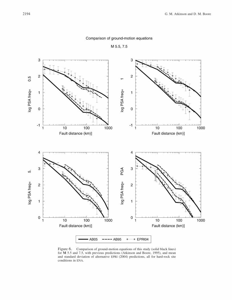
On Figure 6, we compare these new prediction equa-tions with the previous relations of Atkinson and Boore(1995) (table version). The range of new ENA ground-motion prediction equations proposed by EPRI (2004) isalso shown; the EPRI prediction equations are representedby a set of 12 alternative equations with weights, which we
have simplified for plotting by showing the mean and stan-dard deviation of the predictions from the 12 relations. Ournew prediction equations are similar to the AB95 predictionequations. The main difference is that high-frequency am-plitudes (f � 5 Hz) are less than previously predicted (byabout a factor of 1.6 within 100 km), because of a slightlylower average stress parameter (140 bars versus 180 bars)and a steeper near-source attenuation. Our model now in-cludes a small amount of amplification for hard-rock sites,which offsets to some extent the differences due to the fac-tors listed previously. The model also features a higherkappa in comparison with our previous model (j0 � 0.005versus fmax [high-cut filter] � 50 Hz). However, we per-formed parametric sensitivity studies that showed that, withthe exception of predicted ground motions for f � 20Hz, theresults are not sensitive to the choice of a kappa distributionfrom 0.002 to 0.008, versus the use of a fixed fmax � 50 Hz.The reason is that a damped oscillator responds to frequen-cies at or below its natural frequency. The influence of en-ergy at lower frequencies results in the response spectra pre-dictions, and the PGA prediction, being insensitive to kappaover our frequency range of interest. Thus the choice ofkappa is not important and not a factor in the differencesbetween our current predictions and those of AB95.
The new model can be used to predict ground motionsmuch closer to the fault (this is applicable for large eventsthat may rupture to the surface), due to the improved con-sideration of finite-fault effects; however, remember that thevalues at close distances (�10 km) are model based ratherthan empirically driven. The treatment of finite-fault effectsis also important in providing an improved scaling of mo-tions with magnitude, in particular, at closer distances. Wenote that the magnitude/distance saturation effects predictedby the simulations are in qualitative accord with effects seenin empirical databases from active tectonic regions (Booreand Atkinson, 2006). In detail, though, the empirical satu-ration effects are stronger than those predicted by our sim-ulations, in particular, for large magnitudes (M � 7) at dis-tances within 50 km. The new model also explicitly providessite-amplification factors for a full range of shear-wave ve-locities, as described in the next section, leading to less am-biguity in interpretation of the results for soil sites. The over-all similarity of the new prediction equations to those ofAtkinson and Boore (1995) is interesting, given the increasein database and new simulation methodology used in thisstudy. It lends weight to previous conclusions that a two-corner point-source model can be used to mimic salientfinite-fault effects in the development of ground-motion pre-diction equations (Atkinson and Silva, 2000).
It is critical to compare the predicted ground motionswith observations to assess their overall reliability. We com-piled response spectra data for rock sites in ENA, based ondata presented by Atkinson and Boore (1998), Atkinson andChen (1997), and Atkinson (2004). In addition, the Bhuj,India, observations of Cramer and Kumar (2003) are in-cluded, corrected to hard-rock site conditions by using the

2192
Tab
le6
Coe
ffici
ents
ofE
quat
ions
for
Pred
ictin
gM
edia
nE
NA
Gro
und
Mot
ions
onH
ard
Roc
k(H
oriz
onta
lCom
pone
nt,l
og(1
0)V
alue
sA
reG
iven
incg
sU
nits
)fo
r5%
Dam
ped
PSA
atSt
ated
Freq
uenc
ies,
Acc
ordi
ngto
Equ
atio
n(5
)
Freq
uenc
y(H
z)Pe
riod
(sec
)c 1
c 2c 3
c 4c 5
c 6c 7
c 8c 9
c 10
0.20
5.00
�5.
41E
�00
1.71
E�
00�
9.01
E�
2�
2.54
E�
002.
27E
�01
�1.
27E
�00
1.16
E�
019.
79E
�01
�1.
77E
�01
�1.
76E
�04
0.25
4.00
�5.
79E
�00
1.92
E�
00�
1.07
E�
01�
2.44
E�
002.
11E
�01
�1.
16E
�00
1.02
E�
011.
01E
�00
�1.
82E
�01
�2.
01E
�04
0.32
3.13
�6.
04E
�00
2.08
E�
00�
1.22
E�
01�
2.37
E�
002.
00E
�01
�1.
07E
�00
8.95
E�
021.
00E
�00
�1.
80E
�01
�2.
31E
�04
0.40
2.50
�6.
17E
�00
2.21
E�
00�
1.35
E�
01�
2.30
E�
001.
90E
�01
�9.
86E
�01
7.86
E�
029.
68E
�01
�1.
77E
�01
�2.
82E
�04
0.50
2.00
�6.
18E
�00
2.30
E�
00�
1.44
E�
01�
2.22
E�
001.
77E
�01
�9.
37E
�01
7.07
E�
029.
52E
�01
�1.
77E
�01
�3.
22E
�04
0.63
1.59
�6.
04E
�00
2.34
E�
00�
1.50
E�
01�
2.16
E�
001.
66E
�01
�8.
70E
�01
6.05
E�
029.
21E
�01
�1.
73E
�01
�3.
75E
�04
0.80
1.25
�5.
72E
�00
2.32
E�
00�
1.51
E�
01�
2.10
E�
001.
57E
�01
�8.
20E
�01
5.19
E�
028.
56E
�01
�1.
66E
�01
�4.
33E
�04
1.0
1.00
�5.
27E
�00
2.26
E�
00�
1.48
E�
01�
2.07
E�
001.
50E
�01
�8.
13E
�01
4.67
E�
028.
26E
�01
�1.
62E
�01
�4.
86E
�04
1.3
0.79
4�
4.60
E�
002.
13E
�00
�1.
41E
�01
�2.
06E
�00
1.47
E�
01�
7.97
E�
014.
35E
�02
7.75
E�
01�
1.56
E�
01�
5.79
E�
041.
60.
629
�3.
92E
�00
1.99
E�
00�
1.31
E�
01�
2.05
E�
001.
42E
�01
�7.
82E
�01
4.30
E�
027.
88E
�01
�1.
59E
�01
�6.
95E
�04
2.0
0.50
0�
3.22
E�
001.
83E
�00
�1.
20E
�01
�2.
02E
�00
1.34
E�
01�
8.13
E�
014.
44E
�02
8.84
E�
01�
1.75
E�
01�
7.70
E�
042.
50.
397
�2.
44E
�00
1.65
E�
00�
1.08
E�
01�
2.05
E�
001.
36E
�01
�8.
43E
�01
4.48
E�
027.
39E
�01
�1.
56E
�01
�8.
51E
�04
3.2
0.31
5�
1.72
E�
001.
48E
�00
�9.
74E
�02
�2.
08E
�00
1.38
E�
01�
8.89
E�
014.
87E
�02
6.10
E�
01�
1.39
E�
01�
9.54
E�
044.
00.
251
�1.
12E
�00
1.34
E�
00�
8.72
E�
02�
2.08
E�
001.
35E
�01
�9.
71E
�01
5.63
E�
026.
14E
�01
�1.
43E
�01
�1.
06E
�03
5.0
0.19
9�
6.15
E�
011.
23E
�00
�7.
89E
�02
�2.
09E
�00
1.31
E�
01�
1.12
E�
006.
79E
�02
6.06
E�
01�
1.46
E�
01�
1.13
E�
036.
30.
158
�1.
46E
�01
1.12
E�
00�
7.14
E�
02�
2.12
E�
001.
30E
�01
�1.
30E
�00
8.31
E�
025.
62E
�01
�1.
44E
�01
�1.
18E
�03
8.0
0.12
52.
14E
�01
1.05
E�
00�
6.66
E�
02�
2.15
E�
001.
30E
�01
�1.
61E
�00
1.05
E�
014.
27E
�01
�1.
30E
�01
�1.
15E
�03
10.0
0.10
04.
80E
�01
1.02
E�
00�
6.40
E�
02�
2.20
E�
001.
27E
�01
�2.
01E
�00
1.33
E�
013.
37E
�01
�1.
27E
�01
�1.
05E
�03
12.6
0.07
96.
91E
�01
9.97
E�
01�
6.28
E�
02�
2.26
E�
001.
25E
�01
�2.
49E
�00
1.64
E�
012.
14E
�01
�1.
21E
�01
�8.
47E
�04
15.9
0.06
39.
11E
�01
9.80
E�
01�
6.21
E�
02�
2.36
E�
001.
26E
�01
�2.
97E
�00
1.91
E�
011.
07E
�01
�1.
17E
�01
�5.
79E
�04
20.0
0.05
01.
11E
�00
9.72
E�
01�
6.20
E�
02�
2.47
E�
001.
28E
�01
�3.
39E
�00
2.14
E�
01�
1.39
E�
01�
9.84
E�
02�
3.17
E�
0425
.20.
040
1.26
E�
009.
68E
�01
�6.
23E
�02
�2.
58E
�00
1.32
E�
01�
3.64
E�
002.
28E
�01
�3.
51E
�01
�8.
13E
�02
�1.
23E
�04
31.8
0.03
11.
44E
�00
9.59
E�
01�
6.28
E�
02�
2.71
E�
001.
40E
�01
�3.
73E
�00
2.34
E�
01�
5.43
E�
01�
6.45
E�
02�
3.23
E�
0540
.00.
025
1.52
E�
009.
60E
�01
�6.
35E
�02
�2.
81E
�00
1.46
E�
01�
3.65
E�
002.
36E
�01
�6.
54E
�01
�5.
50E
�02
�4.
85E
�05
PGA
0.01
09.
07E
�01
9.83
E�
01�
6.60
E�
02�
2.70
E�
001.
59E
�01
�2.
80E
�00
2.12
E�
01�
3.01
E�
01�
6.53
E�
02�
4.48
E�
04PG
V0.
011
�1.
44E
�00
9.91
E�
01�
5.85
E�
02�
2.70
E�
002.
16E
�01
�2.
44E
�00
2.66
E�
018.
48E
�02
�6.
93E
�02
�3.
73E
�04
Tot
alsi
gma
�0.
30fo
ral
lfr
eque
ncie
s.
Earthquake Ground-Motion Prediction Equations for Eastern North America 2193
Figure 5. Example of regression residuals versus distance for M 6. Gray dots areindividual residuals (where log residual � log simulated PSA — log PSA predicted byequation 5). Filled symbols show mean residuals and standard deviation in distance bins.
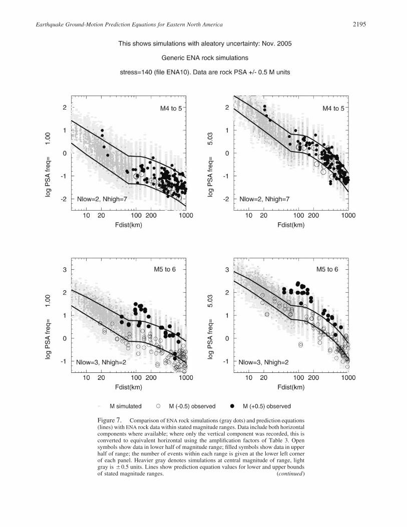
The ENA data (horizontal component or equivalent)have been plotted on Figure 7 in comparison with theground-motion prediction equations (simulations and equa-tions), at two representative frequencies (1 and 5 Hz). Theprediction equations appear to be in reasonable agreementwith the data, with some exceptions. Most notably, the equa-tions underpredict a cluster of enhanced high-frequency am-plitude data for M 5.5 (�0.5) near 100 km. This clusterrepresents strong-motion observations from the M 5.8 1988
site-condition factors adopted for this study (as described inthe next section). The Bhuj data (26 January 2000) are in-cluded because of the suggested similarity of the Bhuj andNew Madrid earthquakes (Cramer and Kumar, 2003; Bodinand Horton, 2004; Singh et al., 2004), but their relevance isless certain than that of the other data, in particular, in lightof the need to make site corrections to obtain equivalentvalues for hard-rock conditions. E The ENA response spec-tra data are provided in the electronic edition of BSSA.
2194 G. M. Atkinson and D. M. Boore
Figure 6. Comparison of ground-motion equations of this study (solid black lines)for M 5.5 and 7.5, with previous predictions (Atkinson and Boore, 1995), and meanand standard deviation of alternative EPRI (2004) predictions, all for hard-rock siteconditions in ENA.
Earthquake Ground-Motion Prediction Equations for Eastern North America 2195
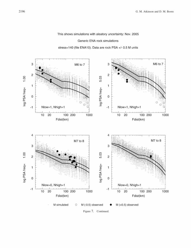
Figure 7. Comparison of ENA rock simulations (gray dots) and prediction equations(lines) with ENA rock data within stated magnitude ranges. Data include both horizontalcomponents where available; where only the vertical component was recorded, this isconverted to equivalent horizontal using the amplification factors of Table 3. Opensymbols show data in lower half of magnitude range; filled symbols show data in upperhalf of range; the number of events within each range is given at the lower left cornerof each panel. Heavier gray denotes simulations at central magnitude of range, lightgray is �0.5 units. Lines show prediction equation values for lower and upper boundsof stated magnitude ranges. (continued)
2196 G. M. Atkinson and D. M. Boore
Figure 7. Continued.
Earthquake Ground-Motion Prediction Equations for Eastern North America 2197
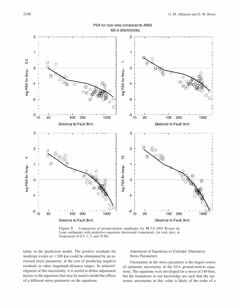
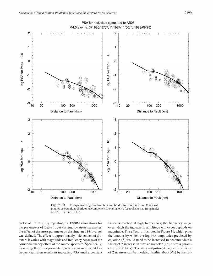
It is illuminating to examine in more detail the data fromthe moderate events that appear to have significant averageresiduals at distances less than 100 km. Figure 9 plots theground-motion amplitudes from the well-recorded M 5.02006 Riviere du Loup earthquake in comparison with theprediction equations of this study. The equations predict thedata well at lower frequencies, but at higher frequenciesthere are positive residuals in the distance range from 30 to70 km. For this event, it appears that the data would prefera higher stress parameter with steeper near-source attenua-tion (although this would overpredict the closest datapoints). On Figure 10, amplitudes are plotted for three eventsof M 4.5 in relation to the prediction equations. The shapeof the attenuation appears approximately correct for theseevents.
Examining the residuals (ratio of observed amplitude topredicted amplitude) indicates that the prediction equationsagree well with available ENA ground-motion data overall:there are near-zero average residuals (within a factor of 1.2)for all frequencies, and there are no statistically significantresidual trends with distance. However, there is a tendencyto positive residuals for moderate events at high frequenciesin the distance range from 30 to 100 km (by as much as afactor of 2), due largely to contributions from the Saguenayand Riviere du Loup events. This indicates epistemic uncer-
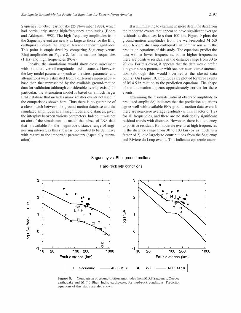
Saguenay, Quebec, earthquake (25 November 1988), whichhad particularly strong high-frequency amplitudes (Booreand Atkinson, 1992). The high-frequency amplitudes fromthe Saguenay event are nearly as large as those for the Bhujearthquake, despite the large difference in their magnitudes.This point is emphasized by comparing Saguenay versusBhuj amplitudes on Figure 8, for intermediate frequencies(1 Hz) and high frequencies (PGA).
Ideally, the simulations would show close agreementwith the data over all magnitudes and distances. However,the key model parameters (such as the stress parameter andattenuation) were estimated from a different empirical data-base than that represented by the available ground-motiondata for validation (although considerable overlap exists). Inparticular, the attenuation model is based on a much largerENA database that includes many smaller events not used inthe comparisons shown here. Thus there is no guarantee ofa close match between the ground-motion database and thesimulated amplitudes at all magnitudes and distances, giventhe interplay between various parameters. Indeed, it was notan aim of the simulations to match the subset of ENA datathat is available for the magnitude-distance range of engi-neering interest, as this subset is too limited to be definitivewith regard to the important parameters (especially attenu-ation).
Figure 8. Comparison of ground-motion amplitudes from M 5.8 Saguenay, Quebec,earthquake and M 7.6 Bhuj, India, earthquake, for hard-rock conditions. Predictionequations of this study are also shown.
2198 G. M. Atkinson and D. M. Boore
Adustment of Equations to Consider AlternativeStress Parameters
Uncertainty in the stress parameter is the largest sourceof epistemic uncertainty in the ENA ground-motion equa-tions. The equations were developed for a stress of 140 bars,but the limitations in our knowledge are such that the epi-stemic uncertainty in this value is likely of the order of a
tainty in the prediction model. The positive residuals formoderate events at �100 km could be eliminated by an in-creased stress parameter, at the cost of producing negativeresiduals in other magnitude-distance ranges. In acknowl-edgment of this uncertainty, it is useful to define adjustmentfactors to the equations that may be used to model the effectsof a different stress parameter on the equations.
Figure 9. Comparison of ground-motion amplitudes for M 5.0 2005 Riviere duLoup earthquake with predictive equations (horizontal component), for rock sites, atfrequencies of 0.5, 1, 5, and 10 Hz.
Earthquake Ground-Motion Prediction Equations for Eastern North America 2199
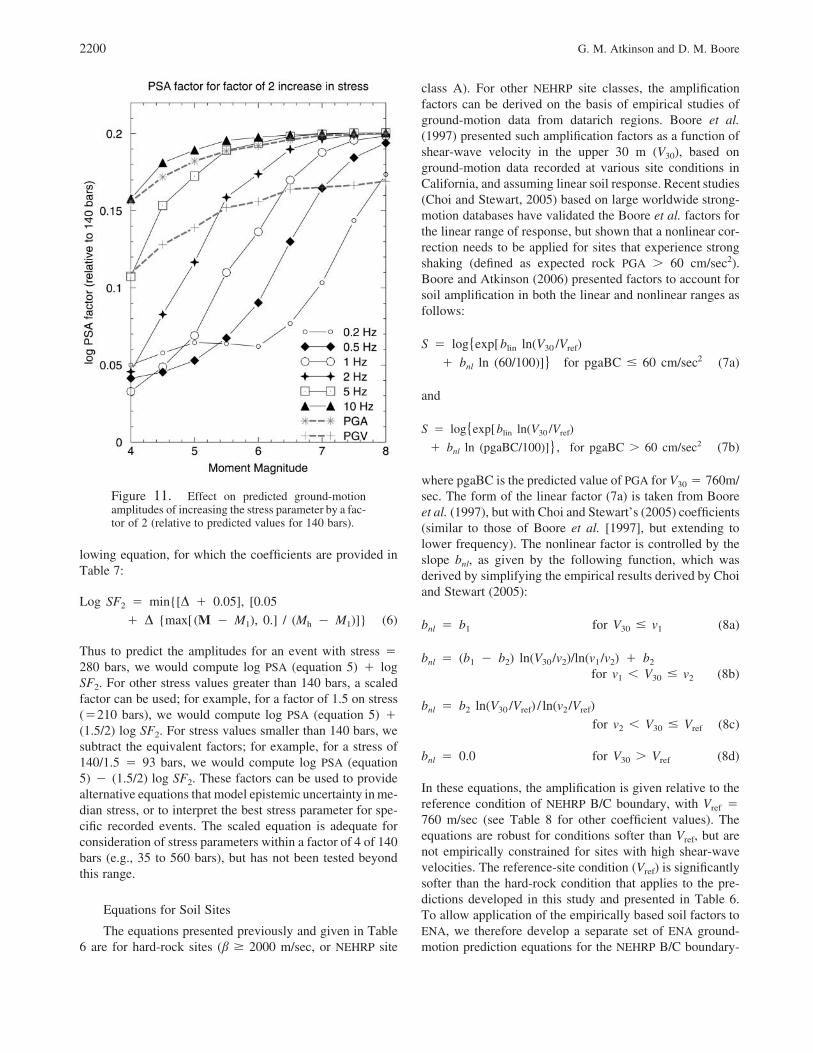
factor is reached at high frequencies; the frequency rangeover which the increase in amplitude will occur depends onmagnitude. The effect is illustrated in Figure 11, which plotsthe amount by which the log PSA amplitudes predicted byequation (5) would need to be increased to accommodate afactor of 2 increase in stress parameter (i.e., a stress param-eter of 280 bars). The stress-adjustment factor for a factorof 2 in stress can be modeled (within about 5%) by the fol-
factor of 1.5 to 2. By repeating the EXSIM simulations forthe parameters of Table 1, but varying the stress parameter,the effect of the stress parameter on the simulated PSA valueswas defined. The effect is approximately independent of dis-tance. It varies with magnitude and frequency because of thecorner-frequency effect of the source spectrum. Specifically,increasing the stress parameter has a near-zero effect at lowfrequencies, then results in increasing PSA until a constant
Figure 10. Comparison of ground-motion amplitudes for four events of M 4.5 withpredictive equations (horizontal component or equivalent), for rock sites, at frequenciesof 0.5, 1, 5, and 10 Hz.
2200 G. M. Atkinson and D. M. Boore
lowing equation, for which the coefficients are provided inTable 7:
Log SF � min{[D � 0.05], [0.052
� D {max[ (M � M ), 0.] / (M � M )]} (6)1 h 1
Thus to predict the amplitudes for an event with stress �280 bars, we would compute log PSA (equation 5) � logSF2. For other stress values greater than 140 bars, a scaledfactor can be used; for example, for a factor of 1.5 on stress(�210 bars), we would compute log PSA (equation 5) �(1.5/2) log SF2. For stress values smaller than 140 bars, wesubtract the equivalent factors; for example, for a stress of140/1.5 � 93 bars, we would compute log PSA (equation5) � (1.5/2) log SF2. These factors can be used to providealternative equations that model epistemic uncertainty in me-dian stress, or to interpret the best stress parameter for spe-cific recorded events. The scaled equation is adequate forconsideration of stress parameters within a factor of 4 of 140bars (e.g., 35 to 560 bars), but has not been tested beyondthis range.
Equations for Soil Sites
The equations presented previously and given in Table6 are for hard-rock sites (b � 2000 m/sec, or NEHRP site
Figure 11. Effect on predicted ground-motionamplitudes of increasing the stress parameter by a fac-tor of 2 (relative to predicted values for 140 bars).
class A). For other NEHRP site classes, the amplificationfactors can be derived on the basis of empirical studies ofground-motion data from datarich regions. Boore et al.(1997) presented such amplification factors as a function ofshear-wave velocity in the upper 30 m (V30), based onground-motion data recorded at various site conditions inCalifornia, and assuming linear soil response. Recent studies(Choi and Stewart, 2005) based on large worldwide strong-motion databases have validated the Boore et al. factors forthe linear range of response, but shown that a nonlinear cor-rection needs to be applied for sites that experience strongshaking (defined as expected rock PGA � 60 cm/sec2).Boore and Atkinson (2006) presented factors to account forsoil amplification in both the linear and nonlinear ranges asfollows:
S � log{exp[b ln(V /V )lin 30 ref2� b ln (60/100)]} for pgaBC � 60 cm/sec (7a)nl
and
S � log{exp[b ln(V /V )lin 30 ref2� b ln (pgaBC/100)]}, for pgaBC � 60 cm/sec (7b)nl
where pgaBC is the predicted value of PGA for V30 � 760m/sec. The form of the linear factor (7a) is taken from Booreet al. (1997), but with Choi and Stewart’s (2005) coefficients(similar to those of Boore et al. [1997], but extending tolower frequency). The nonlinear factor is controlled by theslope bnl, as given by the following function, which wasderived by simplifying the empirical results derived by Choiand Stewart (2005):
b � b for V � v (8a)nl 1 30 1
b � (b � b ) ln(V /v )/ln(v /v ) � bnl 1 2 30 2 1 2 2
for v � V � v (8b)1 30 2
b � b ln(V /V ) / ln(v /V )nl 2 30 ref 2 ref
for v � V � V (8c)2 30 ref
b � 0.0 for V � V (8d)nl 30 ref
In these equations, the amplification is given relative to thereference condition of NEHRP B/C boundary, with Vref �760 m/sec (see Table 8 for other coefficient values). Theequations are robust for conditions softer than Vref, but arenot empirically constrained for sites with high shear-wavevelocities. The reference-site condition (Vref) is significantlysofter than the hard-rock condition that applies to the pre-dictions developed in this study and presented in Table 6.To allow application of the empirically based soil factors toENA, we therefore develop a separate set of ENA ground-motion prediction equations for the NEHRP B/C boundary-
Earthquake Ground-Motion Prediction Equations for Eastern North America 2201
site condition. This involves redoing the simulations, butreplacing the crustal amplification model that is applicableto hard rock (V30 � 2000 m/sec) with one that is applicableto a near-surface velocity of 760 m/sec in ENA; we used themodel given in Table A6 of Frankel et al. (1996), but witha source velocity of 3.7 km/sec rather than 3.6 km/sec. Theamplification model was derived using the square-root-impedance method of Boore and Joyner (1997; see alsoBoore, 2003), in which amplification is computed based onthe seismic-impedance gradient; for each frequency, thedepth corresponding to a quarter wavelength is calculated,and the amplification is estimated based on the square rootof the seismic-impedance ratio between the source regionand the quarter-wavelength depth. Table 4 presents the re-sulting amplification factors.
The amplification factors of Table 4 are multiplied bythe exp(�pfj0) operator in the simulations. For hard-rocksites, j0 was assumed to be uniformly distributed between0.002 and 0.008 (see Table 1). For NEHRP B/C boundary-site conditions, we assume j0 is uniformly distributed be-tween 0.01 and 0.03.
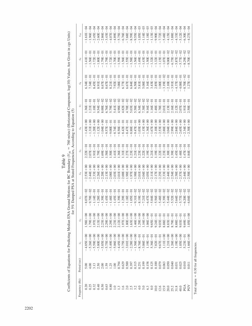
The simulations for NEHRP B/C boundary conditionswere regressed to equation (5) to determine the coefficientsfor the prediction equations as given in Table 9. The predic-tion equations of Table 9 can be used with the soil responsefactors of Boore and Atkinson (2006), as given in equation(7a),(7b) with the coefficients as listed in Table 8, to cal-culate expected ENA ground motions for any specified V30.This makes the implicit assumption that relative amplifica-tion effects of different soil conditions in ENA are the sameas those for active tectonic regions. Note that the stress-amplification factors of equation (6) can be applied to theB/C boundary predictions to consider alternative values ofthe stress parameter.
Figure 12 compares the equations of this study forNEHRP B/C boundary-site conditions with the empirical re-lations of Boore and Atkinson (2006), for active tectonic re-gions, for the same shear-wave velocity. The amplitudes fromthe relations are broadly similar at low frequencies, albeit withvery different functional shapes for the relations. At high fre-quencies, the differences are more pronounced; this study sug-gests that ENA amplitudes scale more strongly with magni-tude at high frequencies than is suggested by empiricalstrong-motion data from active regions. ENA high-frequencyamplitudes are larger than those in active regions, especiallyat large distances (�200 km) and close to the source(�20 km). The empirical relations suggest stronger near-source distance saturation than is provided by the simula-tions of this study; the implication is that the equations forENA may overpredict near-source motions, if there are sig-nificant saturation effects that are not accounted for in thesimulation model. These effects will require further evalu-ation by comparing ENA data more closely with data fromactive tectonic regions.
Table 7Coefficients of Stress Adjustment Factors (Equation 6)
Frequency (Hz) D Ml Mh
0.20 0.15 6.00 8.500.25 0.15 5.75 8.370.32 0.15 5.50 8.250.40 0.15 5.25 8.120.50 0.15 5.00 8.000.63 0.15 4.84 7.700.80 0.15 4.67 7.451.00 0.15 4.50 7.201.26 0.15 4.34 6.951.59 0.15 4.17 6.702.00 0.15 4.00 6.502.52 0.15 3.65 6.373.17 0.15 3.30 6.253.99 0.15 2.90 6.125.02 0.15 2.50 6.006.32 0.15 1.85 5.847.96 0.15 1.15 5.67
10.02 0.15 0.50 5.5012.62 0.15 0.34 5.3415.89 0.15 0.17 5.1720.00 0.15 0.00 5.0025.18 0.15 0.00 5.0031.70 0.15 0.00 5.0039.91 0.15 0.00 5.00PGA 0.15 0.50 5.50PGV 0.11 2.00 5.50
Table 8Coefficients for Soil Response, as Given in Equations (7)
and (8)
Frequency (Hz) blin b1 b2
0.2 �0.752 �0.300 00.25 �0.745 �0.310 00.32 �0.740 �0.330 00.5 �0.730 �0.375 00.63 �0.726 �0.395 01 �0.700 �0.440 01.3 �0.690 �0.465 �0.0021.6 �0.670 �0.480 �0.0312 �0.600 �0.495 �0.0602.5 �0.500 �0.508 �0.0953.2 �0.445 �0.513 �0.1304 �0.390 �0.518 �0.1605 �0.306 �0.521 �0.1856.3 �0.280 �0.528 �0.1858 �0.260 �0.560 �0.140
10 �0.250 �0.595 �0.13212.6 �0.232 �0.637 �0.11715.9 �0.249 �0.642 �0.10520 �0.286 �0.643 �0.10525 �0.314 �0.609 �0.10532 �0.322 �0.618 �0.10840 �0.330 �0.624 �0.115PGA �0.361 �0.641 �0.144PGV �0.600 �0.495 �0.060
At all frequencies, Vref � 760, m1 � 180, m2 � 300.
2202
Tab
le9
Coe
ffici
ents
ofE
quat
ions
for
Pred
ictin
gM
edia
nE
NA
Gro
und
Mot
ions
for
BC
Bou
ndar
y(V
30�
760
m/s
ec)
(Hor
izon
talC
ompo
nent
,log
(10)
Val
ues
Are
Giv
enin
cgs
Uni
ts)
for
5%D
ampe
dPS
Aat
Stat
edFr
eque
ncie
s,A
ccor
ding
toE
quat
ion
(5)
Freq
uenc
y(H
z)Pe
riod
(sec
)c 1
c 2c 3
c 4c 5
c 6c 7
c 8c 9
c 10
0.20
5.00
�4.
85E
�00
1.58
E�
00�
8.07
E�
02�
2.53
E�
002.
22E
�01
�1.
43E
�00
1.36
E�
016.
34E
�01
�1.
41E
�01
�1.
61E
�04
0.25
4.00
�5.
26E
�00
1.79
E�
00�
9.79
E�
02�
2.44
E�
002.
07E
�01
�1.
31E
�00
1.21
E�
017.
34E
�01
�1.
56E
�01
�1.
96E
�04
0.32
3.13
�5.
59E
�00
1.97
E�
00�
1.14
E�
01�
2.33
E�
001.
91E
�01
�1.
20E
�00
1.10
E�
018.
45E
�01
�1.
72E
�01
�2.
45E
�04
0.40
2.50
�5.
80E
�00
2.13
E�
00�
1.28
E�
01�
2.26
E�
001.
79E
�01
�1.
12E
�00
9.54
E�
028.
91E
�01
�1.
80E
�01
�2.
60E
�04
0.50
2.00
�5.
85E
�00
2.23
E�
00�
1.39
E�
01�
2.20
E�
001.
69E
�01
�1.
04E
�00
8.00
E�
028.
67E
�01
�1.
79E
�01
�2.
86E
�04
0.63
1.59
�5.
75E
�00
2.29
E�
00�
1.45
E�
01�
2.13
E�
001.
58E
�01
�9.
57E
�01
6.76
E�
028.
67E
�01
�1.
79E
�01
�3.
43E
�04
0.80
1.25
�5.
49E
�00
2.29
E�
00�
1.48
E�
01�
2.08
E�
001.
50E
�01
�9.
00E
�01
5.79
E�
028.
21E
�01
�1.
72E
�01
�4.
07E
�04
1.0
1.00
�5.
06E
�00
2.23
E�
00�
1.45
E�
01�
2.03
E�
001.
41E
�01
�8.
74E
�01
5.41
E�
027.
92E
�01
�1.
70E
�01
�4.
89E
�04
1.3
0.79
4�
4.45
E�
002.
12E
�00
�1.
39E
�01
�2.
01E
�00
1.36
E�
01�
8.58
E�
014.
98E
�02
7.08
E�
01�
1.59
E�
01�
5.75
E�
041.
60.
629
�3.
75E
�00
1.97
E�
00�
1.29
E�
01�
2.00
E�
001.
31E
�01
�8.
42E
�01
4.82
E�
026.
77E
�01
�1.
56E
�01
�6.
76E
�04
2.0
0.50
0�
3.01
E�
001.
80E
�00
�1.
18E
�01
�1.
98E
�00
1.27
E�
01�
8.47
E�
014.
70E
�02
6.67
E�
01�
1.55
E�
01�
7.68
E�
042.
50.
397
�2.
28E
�00
1.63
E�
00�
1.05
E�
01�
1.97
E�
001.
23E
�01
�8.
88E
�01
5.03
E�
026.
84E
�01
�1.
58E
�01
�8.
59E
�04
3.2
0.31
5�
1.56
E�
001.
46E
�00
�9.
31E
�02
�1.
98E
�00
1.21
E�
01�
9.47
E�
015.
58E
�02
6.50
E�
01�
1.56
E�
01�
9.55
E�
044.
00.
251
�8.
76E
�01
1.29
E�
00�
8.19
E�
02�
2.01
E�
001.
23E
�01
�1.
03E
�00
6.34
E�
025.
81E
�01
�1.
49E
�01
�1.
05E
�03
5.0
0.19
9�
3.06
E�
011.
16E
�00
�7.
21E
�02
�2.
04E
�00
1.22
E�
01�
1.15
E�
007.
38E
�02
5.08
E�
01�
1.43
E�
01�
1.14
E�
036.
30.
158
1.19
E�
011.
06E
�00
�6.
47E
�02
�2.
05E
�00
1.19
E�
01�
1.36
E�
009.
16E
�02
5.16
E�
01�
1.50
E�
01�
1.18
E�
038.
00.
125
5.36
E�
019.
65E
�01
�5.
84E
�02
�2.
11E
�00
1.21
E�
01�
1.67
E�
001.
16E
�01
3.43
E�
01�
1.32
E�
01�
1.13
E�
0310
.00.
100
7.82
E�
019.
24E
�01
�5.
56E
�02
�2.
17E
�00
1.19
E�
01�
2.10
E�
001.
48E
�01
2.85
E�
01�
1.32
E�
01�
9.90
E�
0412
.60.
079
9.67
E�
019.
03E
�01
�5.
48E
�02
�2.
25E
�00
1.22
E�
01�
2.53
E�
001.
78E
�01
1.00
E�
01�
1.15
E�
01�
7.72
E�
0415
.90.
063
1.11
E�
008.
88E
�01
�5.
39E
�02
�2.
33E
�00
1.23
E�
01�
2.88
E�
002.
01E
�01
�3.
19E
�02
�1.
07E
�01
�5.
48E
�04
20.0
0.05
01.
21E
�00
8.83
E�
01�
5.44
E�
02�
2.44
E�
001.
30E
�01
�3.
04E
�00
2.13
E�
01�
2.10
E�
01�
9.00
E�
02�
4.15
E�
0425
.20.
040
1.26
E�
008.
79E
�01
�5.
52E
�02
�2.
54E
�00
1.39
E�
01�
2.99
E�
002.
16E
�01
�3.
91E
�01
�6.
75E
�02
�3.
88E
�04
31.8
0.03
11.
19E
�00
8.88
E�
01�
5.64
E�
02�
2.58
E�
001.
45E
�01
�2.
84E
�00
2.12
E�
01�
4.37
E�
01�
5.87
E�
02�
4.33
E�
0440
.00.
025
1.05
E�
009.
03E
�01
�5.
77E
�02
�2.
57E
�00
1.48
E�
01�
2.65
E�
002.
07E
�01
�4.
08E
�01
�5.
77E
�02
�5.
12E
�04
PGA
0.01
05.
23E
�01
9.69
E�
01�
6.20
E�
02�
2.44
E�
001.
47E
�01
�2.
34E
�00
1.91
E�
01�
8.70
E�
02�
8.29
E�
02�
6.30
E�
04PG
V0.
011
�1.
66E
�00
1.05
E�
00�
6.04
E�
02�
2.50
E�
001.
84E
�01
�2.
30E
�00
2.50
E�
011.
27E
�01
�8.
70E
�02
�4.
27E
�04
Tot
alsi
gma
�0.
30fo
ral
lfr
eque
ncie
s.
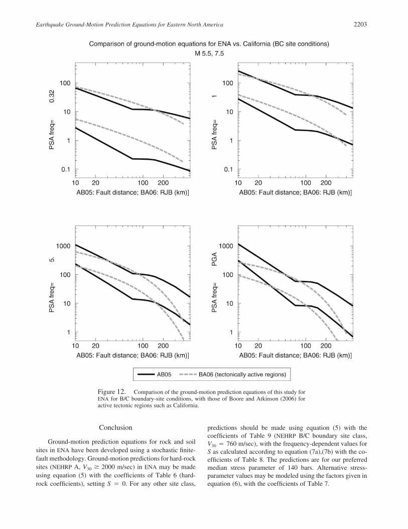
Earthquake Ground-Motion Prediction Equations for Eastern North America 2203
Conclusion
Ground-motion prediction equations for rock and soilsites in ENA have been developed using a stochastic finite-fault methodology. Ground-motion predictions for hard-rocksites (NEHRP A, V30 � 2000 m/sec) in ENA may be madeusing equation (5) with the coefficients of Table 6 (hard-rock coefficients), setting S � 0. For any other site class,
predictions should be made using equation (5) with thecoefficients of Table 9 (NEHRP B/C boundary site class,V30 � 760 m/sec), with the frequency-dependent values forS as calculated according to equation (7a),(7b) with the co-efficients of Table 8. The predictions are for our preferredmedian stress parameter of 140 bars. Alternative stress-parameter values may be modeled using the factors given inequation (6), with the coefficients of Table 7.
Figure 12. Comparison of the ground-motion prediction equations of this study forENA for B/C boundary-site conditions, with those of Boore and Atkinson (2006) foractive tectonic regions such as California.
2204 G. M. Atkinson and D. M. Boore
Acknowledgments
This work was financially supported by the U.S. Geological SurveyNational Earthquake Hazards Reduction Program (Grant 02HQGR0001),and by the U.S. Nuclear Regulatory Commission. We thank Chris Cramerand Ken Campbell for constructive reviews.
References
Abrahamson, N., and W. Silva (1997). Empirical response spectral atten-uation relations for shallow crustal earthquakes, Seism. Res. Lett. 68,94–127.
Aki, K. (1967). Scaling law of seismic spectrum, J. Geophys. Res. 72,1217–1231.
Anderson, J., and S. Hough (1984). A model for the shape of the Fourieramplitude spectrum of acceleration at high frequencies, Bull. Seism.Soc. Am. 74, 1969–1993.
Atkinson, G. (1993a). Source spectra for earthquakes in eastern NorthAmerica, Bull. Seism. Soc. Am. 83, 1778–1798.
Atkinson, G. (1993b). Notes on ground motion parameters for eastern NorthAmerica: duration and H/V ratio, Bull. Seism. Soc. Am. 83, 587–596.
Atkinson, G. (1996). The high-frequency shape of the source spectrum forearthquakes in eastern and western Canada, Bull. Seism. Soc. Am. 86,106–112.
Atkinson, G. (2004). Empirical attenuation of ground motion spectral am-plitudes in southeastern Canada and the northeastern United States,Bull. Seism. Soc. Am. 94, 1079–1095.
Atkinson, G., and D. Boore (1995). New ground motion relations for east-ern North America, Bull. Seism. Soc. Am. 85, 17–30.
Atkinson, G., and D. Boore (1997). Stochastic point-source modeling ofground motions in the Cascadia region, Seism. Res. Lett. 68, 74–85.
Atkinson, G., and D. Boore (1998). Evaluation of models for earthquakesource spectra in eastern North America, Bull. Seism. Soc. Am. 88,917–934.
Atkinson, G., and J. Cassidy (2000). Integrated use of seismograph andstrong motion data to determine soil amplification in the Fraser Delta:results from the Duvall and George Strait earthquakes, Bull. Seism.Soc. Am. 90, 1028–1040.
Atkinson, G., and S. Chen (1997). Regional seismograms from historicalearthquakes in southeastern Canada, Seism. Res. Lett. 68, 797–807.
Atkinson, G., and R. Mereu (1992). The shape of ground motion attenuationcurves in southeastern Canada, Bull. Seism. Soc. Am. 82, 2014–2031.
Atkinson, G., and W. Silva (1997). Empirical source spectra for Californiaearthquakes, Bull. Seism. Soc. Am. 87, 97–113.
Atkinson, G., and W. Silva (2000). Stochastic modeling of Californiaground motions, Bull. Seism. Soc. Am. 90, 255–274.
Beresnev, I., and G. Atkinson (1997a). Modeling finite fault radiation fromthe xn spectrum, Bull. Seism. Soc. Am. 87, 67–84.
Beresnev, I., and G. Atkinson (1997b). Shear wave velocity survey of seis-mographic sites in eastern Canada: Calibration of empirical regressionmethod of estimating site response, Seism. Res. Lett. 68, 981–987.
Beresnev, I., and G. Atkinson (1998a). Stochastic finite-fault modeling ofground motions from the 1994 Northridge, California earthquake, partI: Validation on rock sites, Bull. Seism. Soc. Am. 88, 1392–1401.
Beresnev, I., and G. Atkinson (1998b). FINSIM—a FORTRAN program forsimulating stochastic acceleration time histories from finite faults,Seism. Res. Lett. 69, 27–32.
Beresnev, I., and G. Atkinson (2002). Source parameters of earthquakes ineastern and western North America based on finite-fault modeling,Bull. Seism. Soc. Am. 92, 695–710.
Bodin, P., and S. Horton (2004). Source parameters and tectonic implica-tions of aftershocks of the Mw 7.6 Bhuj earthquake of January 26,2001, Bull. Seism. Soc. Am. 94, 818–827.
Boore, D. (1983). Stochastic simulation of high-frequency ground motionsbased on seismological models of the radiated spectra, Bull. Seism.Soc. Am. 73, 1865–1894.
Boore, D. (2003). Prediction of ground motion using the stochastic method,Pure Appl. Geophys. 160, 635–676.
Boore, D. (2004). Can site response be predicted? J. Earthquake Eng. 8(Special Issue 1), 1–41.
Boore, D., and G. Atkinson (1992). Source spectra for the 1988 Saguenay,Quebec earthquakes, Bull. Seism. Soc. Am. 82, 683–719.
Boore, D., and G. Atkinson (2006). Boore-Atkinson NGA EmpiricalGround Motion Model for the Average Horizontal Component ofPGA, PGV and SA at Spectral Periods of 0.1, 0.2, 1, 2, and 3 Seconds,www.peer.berkeley.edu (last accessed June 2006).
Boore, D., and W. Joyner (1997). Site amplifications for generic rock sites,Bull. Seism. Soc. Am. 87, 327–341.
Boore, D., W. Joyner, and T. Fumal (1997). Equations for estimating hor-izontal response spectra and peak acceleration from western NorthAmerican earthquakes: a summary of recent work, Seism. Res. Lett.68, 128–153.
Brune, J. (1970). Tectonic stress and the spectra of seismic shear wavesfrom earthquakes, J. Geophys. Res. 75, 4997–5009.
Brune, J. (1971). Correction, J. Geophys. Res. 76, 5002.Choi, Y., and J. Stewart (2005). Nonlinear site amplification as a function
of 30m shear wave velocity, Earthquake Spectra 21, 1–30.Cramer, C., and A. Kumar (2003). 2001 Bhuj, India earthquake engineering
seismoscope recordings and eastern North America ground motionattenuation relations, Bull. Seism. Soc. Am. 93, 1390–1394.
Electric Power Research Institute (EPRI) (1993). Guidelines for determin-ing design basis ground motions, Early site permit demonstration pro-gram, Vol. 1, RP3302, Electric Power Research Institute, Palo Alto,California.
Electric Power Research Institute (EPRI) (2004). CEUS ground motionproject final report. Technical Report 1009684. Electric Power Re-search Institute, Dominion Energy, Glen Allen, Virginia, Entergy Nu-clear, Jackson, Mississippi; and Exelon Generation Company, Ken-nett Square, Pennsylvania, Palo Alto, California.
Frankel, A., C. Mueller, T. Barnhard, D. Perkins, E. Leyendecker, N. Dick-man, S. Hanson, and M. Hopper (1996). National seismic hazardmaps: documentation June 1996, U.S. Geol. Surv. Open-File Rept.96-532, 69 pp.
Hanks, T., and R. McGuire (1981). The character of high-frequency strongground motion, Bull. Seism. Soc. Am. 71, 2071–2095.
Hartzell, S. (1978). Earthquake aftershocks as Green’s functions, Geophys.Res. Lett. 5, 1–14.
Heaton, T. (1990). Evidence for and implications of self-healing pulses ofslip in earthquake rupture, Phys. Earth Planet. Interiors 64, 1–20.
Heaton, T., and S. Hartzell (1986). Source characteristics of hypotheticalsubduction earthquakes in the Northwestern United States, Bull.Seism. Soc. Am. 76, 675–708.
Hough, S., J. Armbruster, L. Seeber, and J. Hough (2000). On the ModifiedMercalli Intensities and magnitudes of 1811–1812 New Madrid earth-quakes, J. Geophys. Res. 105, 839–864.
Irikura, K. (1983). Semi-empirical estimation of strong ground motionsduring large earthquakes, Bull. Disaster Prevention Res. Inst., KyotoUniv. 33, 63–104.
Johnston, A. (1996). Seismic moment assessment of earthquakes in stablecontinental regions. Part 3: The 1811–1812 New Madrid, 1886Charleston, and 1755 Lisbon earthquakes, Geophys. J. Int. 126, 314–344.
Joyner, W., and D. Boore (1986). On simulating large earthquakes byGreen’s-function addition of smaller earthquakes, in EarthquakeSource Mechanics, Maurice Ewing Series 6, S. Das, et al. (Editors),Am. Geophys. Union, 269–274.
Lermo, J., and F. Chavez-Garcia (1993). Site effect evaluation using spec-tral ratios with only one station, Bull. Seism. Soc. Am. 83, 1574–1594.
Ma, S., and G. Atkinson (2006). Focal depth distribution for earthquakeswith MN � 2.8 in western Quebec, southern Ontario and northernNew York, Bull. Seism. Soc. Am. 96, 609–623
Motazedian, D., and G. Atkinson (2005). Stochastic finite-fault model basedon dynamic corner frequency, Bull. Seism. Soc. Am. 95, 995–1010.
Earthquake Ground-Motion Prediction Equations for Eastern North America 2205
Sadigh, K., C. Chang, J. Egan, F. Makdisi, and R. Youngs (1997). Atten-uation relationships for shallow crustal earthquakes based on Cali-fornia strong motion data, Seism. Res. Lett. 68, 180–189.
Siddiqqi, J., and G. Atkinson (2002). Ground motion amplification at rocksites across Canada, as determined from the horizontal-to-verticalcomponent ratio, Bull. Seism. Soc. Am. 92, 877–884.
Singh, S., J. Pacheco, B. Bansal, X. Perez-Campos, R. Dattatrayam, andG. Suresh (2004). A source study of the Bhuj, India, earthquake of26 January 2001 (Mw 7.6), Bull. Seism. Soc. Am. 94, 1195–1206.
Somerville, P., N. Collins, N. Abrahamson, R. Graves, and C. Saikia(2001). Ground motion attenuation relations for the central and east-ern United States, Report to U.S. Geological Survey, NEHRP ExternalResearch Program, Award No. 99-HQ-GR-0098.
Somerville, P., M. Sen, and B. Cohee (1991). Simulations of strong groundmotions recorded during the 1985 Michoacan, Mexico and Valpa-raiso, Chile, earthquakes, Bull. Seism. Soc. Am. 81, 1–27.
Toro, G., and R. McGuire (1987). Calculational procedures for seismichazard analysis and its uncertainty in the eastern United States, inProc. Third Intl. Conf. Soil Dynamics and Earthquake Eng., Prince-ton, New Jersey, 195–206.
Toro, G., N. Abrahamson, and J. Schneider (1997). Model of strong groundmotion in eastern and central North America: best estimates and un-certainties, Seism. Res. Lett. 68, 41–57.
Tumarkin, A., and R. Archuleta (1994). Empirical ground motion predic-tion, Ann. Geofis. 37, 1691–1720.
Wells, D., and K. Coppersmith (1994). New empirical relationships amongmagnitude, rupture length, rupture width, rupture area, and surfacedisplacement, Bull. Seism. Soc. Am. 84, 974–1002.
Zeng, Y., J. Anderson, and G. Yu (1994). A composite source model forcomputing realistic synthetic strong ground motions, Geophys. Res.Lett. 21, 725–728.
Department of Earth SciencesCarleton UniversityOttawa, Ontario K1S 5B6, [email protected]
(G.M.A.)
U.S. Geological Survey345 Middlefield Rd.Menlo Park, California [email protected]
(D.M.B.)
Manuscript received 5 December 2005.