early warning system europe
TRANSCRIPT

8/3/2019 Early Warning System Europe
http://slidepdf.com/reader/full/early-warning-system-europe 1/67
E U R O P E A N C E N T R A L B A N K
W O R K I N G PA P E R S E R I E S
E C B
E Z B
E K T
B C E
E K P
WORKING PAPER NO. 145
TOWARDS A NEW EARLY
WARNING SYSTEM OF
FINANCIAL CRISES
BY MATTHIEU BUSSIERE AND
MARCEL FRATZSCHER
MAY 2002

8/3/2019 Early Warning System Europe
http://slidepdf.com/reader/full/early-warning-system-europe 2/67
* The paper was written while Matthieu Bussiere was visiting the External Developments Division of the European Central Bank.We have benefited from many discussions and would like to thank in particular Mike Artis, Anindya Banerjee, Gonzalo Camba Méndez, Søren Johansen, Helmut Lütkepohl, Rasmus Rüffer, Bernd Schnatz and the participants of two ECB seminars for their comments and suggestions.The views expressed in this paper are those of the authors and do not necessarily reflect those of the European Central Bank.
** [email protected] ; European University Institute, Badia Fiesolana,I-50016 San Domenico (FI),Italy.*** [email protected] ; European Central Bank, External Developments Division, Kaiserstrasse 29, D-60311 Frankfurt, Germany.
WORKING PAPER NO. 145
TOWARDS A NEW EARLY
WARNING SYSTEM OF
FINANCIAL CRISES*
BY MATTHIEU BUSSIERE** AND
MARCEL FRATZSCHER***
MAY 2002
E U R O P E A N C E N T R A L B A N K
W O R K I N G PA P E R S E R I E S
8/3/2019 Early Warning System Europe
http://slidepdf.com/reader/full/early-warning-system-europe 3/67
© European Central Bank, 2002
Address Kaiserstrasse 29
D-60311 Frankfurt am Main
Germany Postal address Postfach 16 03 19
D-60066 Frankfurt am Main
Germany
Telephone +49 69 1344 0
Internet http://www.ecb.int
Fax +49 69 1344 6000
Telex 411 144 ecb d
All rights reserved.
Reproduction for educational and non-commercial purposes is permitted provided that the source is acknowledged.
The views expressed in this paper are those of the authors and do not necessarily reflect those of the European Central Bank.
ISSN 1561-0810
8/3/2019 Early Warning System Europe
http://slidepdf.com/reader/full/early-warning-system-europe 4/67
ECB Work ing Paper No 14 5 • May 2002 3
Contents
Abstract 4
Non-Technical Summary 5
1 Introduction 7
2 Existing methodological approaches of EWS models 9
2.1 What is the aim of EWS models? 9
2.2 Existing empirical models of currency crises 10
2.3 Evaluating the perfor mance of EWS models: The trade-off problem 13
3 Estimating the binomial logit model 14
3.1 The data 14
3.2 Results and performance of the pooled logit model 153.3 Panel data analysis 18
4 A multinomial logit EWS approach 19
4.1 Explaining the post-crisis bias 19
4.2 How to address the post-crisis bias 20
5 Mult inomial logit EWS model: Results and robustness tests 24
5.1 Results and performance of the multinomial logit model 24
5.2 Discussion of results 25
5.3 Robustness tests 26
5.4 Out-of-sample performance 29
6 Policy relevance of the multinomial logit EWS model 32
6.1 Loss function for the policy-maker 32
6.2 Solving for the optimal threshold and time horizon 33
6.3 Illustrating the signal distr ibution for time-horizon models 36
7 Conclusions 38
References 40
Appendix 43
Appendix 1: Country list and data sources 43
Appendix 2: Discussion of defini tion and explanatory power of independent variables 46
Appendix 3: Estimation results with alternative models 50
Appendix 4: Robustness tests and sensitivity analysis 51
Appendix 5: Event analysis 53
Appendix 6: Predicted probabilit ies and signal extraction 56
European Central Bank Working Paper Series 58
8/3/2019 Early Warning System Europe
http://slidepdf.com/reader/full/early-warning-system-europe 5/67
Abstract
This paper develops a new Early Warning System (EWS) model for predicting financial crises, based
on a multinomial logit model. It is shown that EWS approaches based on binomial discrete-dependent-
variable models can be subject to what we call a post-crisis bias. This bias arises when no distinction
is made between tranquil periods, when economic fundamentals are largely sound and sustainable, and
crisis/post-crisis periods, when economic variables go through an adjustment process before reaching
a more sustainable level or growth path. We show that applying a multinomial logit model, which
allows distinguishing between more than two states, is a valid way of solving this problem and
constitutes a substantial improvement in the ability to forecast financial crises. The empirical results
reveal that, for a set of 32 open emerging markets from 1993 till the present, the model would have
correctly predicted a large majority of crises in emerging markets. Moreover, we derive general results
about the optimal design of EWS models, which allows policy-makers to make an optimal choice
based on their degree of risk-aversion against unanticipated financial crises.
JEL classification: F31, F47, F30.Keywords: currency crises; Early Warning System; crisis prediction.
ECB • Work in g Paper No 145 • May 20024
8/3/2019 Early Warning System Europe
http://slidepdf.com/reader/full/early-warning-system-europe 6/67
ECB • Work ing Paper No 14 5 • May 2002 5
Non-Technical Summary
The last decade saw a large number of financial crises in emerging market economies (EMEs)
with often devastating economic, social and political consequences. These financial criseswere in many cases not confined to individual economies but spread contagiously to other
markets as well. As a result, international financial institutions have developed Early Warning
System (EWS) models, with the aim of identifying economic weaknesses and vulnerabilities
among emerging markets and ultimately anticipating such events.
The aim of this paper is to present a new EWS model that significantly improves upon
existing models. First, the paper develops a different empirical methodology that corrects for
what we call a post-crisis bias. This bias arises if models fail to distinguish between tranquil
periods, when economic fundamentals are largely sound and sustainable, and post-
crisis/recovery periods, when economic variables go through an adjustment process before
reaching a more sustainable level or growth path. We show that making this distinction by
using a multinomial logit model with three regimes (a tranquil regime, a pre-crisis regime,
and a post-crisis/recovery regime) constitutes a substantial improvement in the forecasting
ability of EWS models.
A second aim of this paper is to test for the role of a broad set of economic and financial
variables in financial crises. In particular, we test a number of contagion indicators to measure
real and financial channels of transmission across economies. We find that in particular the
financial contagion channel has been an important factor in explaining and anticipating
currency crises for a set of 32 open EMEs for the period 1993-2001. Overall, the empirical
performance of our EWS model constitutes a significant improvement in comparison to
existing EWS models. Our EWS model based on the multinomial logit would have predicted
most EME financial crises since the early 1990s, while entirely missing a crisis only in one
case.
Finally, the paper derives general results about the optimal design of EWS models for policy-
makers. It shows how changes to the preferences of the policy-maker and the specification of
her loss function can fundamentally alter the optimal design of the EWS model in terms of the
time horizon for the model and the desired policy action. We illustrate how these choices
depend crucially on the trade-off between, on the one hand, issuing many crisis alarms (hence
also sending many false alarms) and, on the other hand, issuing fewer alarms at the expense
of missing some crises. Hence it can be shown how the policy-maker’s preferences and
degree of risk-aversion about this trade-off determines the optimal design of the EWS model.
8/3/2019 Early Warning System Europe
http://slidepdf.com/reader/full/early-warning-system-europe 7/67
ECB • Work in g Paper No 145 • May 20026
From a policy perspective, developing reliable EWS models can be of substantial value by
allowing policy-makers to obtain clear signals as to when and how to take pre-emptive
measures in order to mitigate or even prevent financial turmoil. Although EWS models can
not replace the sound judgment of policy-makers in guiding policy, they can play an
important complementary role as a neutral and objective measure of vulnerability.
8/3/2019 Early Warning System Europe
http://slidepdf.com/reader/full/early-warning-system-europe 8/67
ECB • Work ing Paper No 14 5 • May 2002 7
1 Introduction
The last decade saw a large number of financial crises in emerging market economies (EMEs)
with often devastating economic, social and political consequences. These financial crises were in
many cases not confined to individual economies but spread contagiously to other markets as well. In
particular the Latin American crisis of 1994-95 and the Asian crisis of 1997-98 affected a wide group
of countries and had systemic repercussions for the international financial system as a whole.
As a result, international organizations and also private sector institutions have begun to develop Early
Warning System (EWS) models with the aim of anticipating whether and when individual countries
may be affected by a financial crisis. The IMF has taken a lead in putting significant effort into
developing EWS models for EMEs, resulting in influential papers by Kaminsky, Lizondo and Reinhart
(1998) and by Berg and Pattillo (1999b). But also many central banks, such as the US Federal Reserve(Kamin, Schindler and Samuel, 2001, Kamin and Babson, 1999) and the Bundesbank (Schnatz, 1998,
1999), academics and various private sector institutions have developed models in recent years.
EWS models can have substantial value to policy-makers by allowing them to detect underlying
economic weaknesses and vulnerabilities, and possibly taking pre-emptive steps to reduce the risks of
experiencing a crisis. The central concern is, however, that these models have been shown to perform
only modestly well in predicting crises (Berg and Pattillo, 1999a).
The aim of this paper is to develop a new EWS model that significantly improves upon existing
models in three ways. First, and most importantly, the paper argues that a key weakness of existing
EWS models is that they are subject to what we call a post-crisis bias. This bias implies that these
models fail to distinguish between tranquil periods, when economic fundamentals are largely sound
and sustainable, and post-crisis/recovery periods, when economic variables go through an adjustment
process before reaching a more sustainable level or growth path. We show that making this distinction
by using a multinomial logit model with three regimes (a tranquil regime, a pre-crisis regime, and
post-crisis/recovery regime) constitutes a substantial improvement in the forecasting ability of EWS
models.
Second, many financial crises since the 1990s have been contagious in spreading across markets.
Another aim of this paper is therefore to apply to EWS models contagion indicators, developed in
Fratzscher (1998, 2002), to measure real contagion channels through trade linkages (direct and
indirect) and financial contagion channels via equity market interdependence. We find that in
particular the financial contagion channel has been an important factor in explaining and anticipating
currency crises.
8/3/2019 Early Warning System Europe
http://slidepdf.com/reader/full/early-warning-system-europe 9/67
Third, this paper uses a data sample of 32 EMEs, with monthly frequency, for the period 1993-2001 as
the basis for the EWS model estimations. Since the aim of an EWS model is to develop a framework
that allows predicting financial crises in relatively open economies in the future, it is imperative to use
for the in-sample estimation only those crises and country observations that are similar to those that
are likely to occur in the future. We have therefore started our sample only in 1993, excluding the
1980’s and early 1990’s, during which capital markets were not yet integrated and capital accounts
often still closed to foreign investors, also because many countries still experienced hyperinflation in
the early 1990’s. Likewise, we have excluded the years immediately following the transition to a free
market in the Eastern European countries.
The empirical performance of our EWS model constitutes a significant improvement in comparison to
existing EWS models. In particular, the use of the multinomial logit model reduces substantially the
number of false signals (i.e. the number of times the model indicates that a crisis is likely to occur but
no crisis actually happens) and of missed crises (i.e. when the model issues no signal but a crisis
occurs). Overall, the EWS model based on the multinomial logit would have predicted most EME
financial crises since the early 1990s, while entirely missing a crisis only in one case.
Finally, the paper derives general results about the optimal design of EWS models. It shows how
changes to the preferences of the policy-maker and the specification of her loss function can
fundamentally alter the optimal design of the EWS model a policy-maker may wish to choose. On theone hand, taking pre-emptive action in response to a signal about a possible crisis is costly from a
policy-maker’s perspective. But on the other hand, also not receiving a signal when a crisis actually
occurs can be costly if early action by the policy-maker could have helped prevent or at least lessen
the impact of a crisis. We show how the policy-maker’s preferences and degree of risk-aversion about
this trade-off determines the optimal design of the EWS model.
The paper proceeds as follows. Section 2 starts by reviewing the two most commonly used approaches
for EWS models, the leading indicator approach and the discrete-dependent variable approach. Section
3 discusses the results obtained from a simple binomial logit model. Section 4 then discusses the post-
crisis bias and the multinomial logit as a way of solving it. Section 5 presents the results from the
multinomial logit and compares them with alternative models. Section 6 tackles the implications of the
model for optimal policy design and section 7 concludes.
ECB • Work in g Paper No 145 • May 20028
8/3/2019 Early Warning System Europe
http://slidepdf.com/reader/full/early-warning-system-europe 10/67
2 Existing Methodological Approaches of EWS models
2.1 What is the aim of EWS models?
There are various types of financial crises: currency crises, banking crises, sovereign debt crises,
private sector debt crises, equity market crises. The EWS model in this paper, like almost all EWS
models on EMEs in the literature, focuses primarily on currency crises. Currency crises often coincide
or occur in quick succession with other types of crises, for instance together with banking crises or
what has been dubbed the “twin crises” (Kaminsky and Reinhart, 1996). More specifically, our EWS
model looks at successful as well as unsuccessful speculative attacks on currencies by employing a
commonly used exchange market pressure (EMPi,t) variable for defining a currency crisis for each
country i and period t:
÷÷
ø
ö
çç
è
æ −−−+÷
÷
ø
ö
çç
è
æ −=
−
−
−
−
−
1,
1,,
1,,
1,
1,,
, )(t i
t it i
rest it ir
t i
t it i
RERt ires
resresr r
RER
RER RER EMP ω ω ω (1)
EMPi,t is a weighted average of the change of the real effective exchange rate (RER), the change in the
interest rate (r) and the change in foreign exchange reserves (res). Taking the real variables for the
exchange rate and the interest rate is intended to account for differences in inflation rates across
countries and over time. The weights ωRER , ωr and ωres are the relative precision of each variable so as
to give a larger weight to the variables with less volatility. The relative precision is defined as the
inverse of the variance of each variable for all countries over the full sample period 1993-2001.
The rationale for using a weighted average of these three variables is the following. If investors
consider the underlying economic factors as unsustainable or vulnerable and attack a currency, a
government essentially has two options. The first option is to abstain from defending the currency,
either by abandoning a fixed exchange rate regime or by avoiding to intervene in foreign exchange
markets, and to let the currency devalue and markets determine its new price. The second option is to
defend the currency regime, or what is considered an appropriate exchange rate level, by raising
interest rates and running down foreign exchange reserves. EMP i,t allows capturing both cases.
As a next step, we define a currency crisis (CCi,t) as the event when the exchange market pressure
(EMPi,t) variable is two standard deviations (SD) or more above its country average EMP i:
ïî
ïíì +>
=
otherwiseif
EMPSD EMP EMPif CC iit i
t i
0
)(21 ,, (2)
ECB • Work ing Paper No 14 5 • May 2002 9
8/3/2019 Early Warning System Europe
http://slidepdf.com/reader/full/early-warning-system-europe 11/67
ECB • Work in g Paper No 145 • May 200210
This is the definition of currency crises that will be used below in our econometric analysis. It is quite
similar, though not identical, to the measures commonly used in the literature.1
The next crucial issue is the question of what we are trying to predict: the timing of a currency crisis or merely its occurrence? As the state of the literature on EWS models for financial crisis shows, it is
already very challenging to predict reliably whether or not a crisis will occur in a particular country.
Therefore, predicting not only whether a currency crisis happens but also the timing when it will
happen is a highly ambitious goal and has, to our knowledge, not been undertaken so far.
The objective of our EWS is therefore not to predict the exact timing of a crisis, but to predict whether
a crisis occurs within a specific time horizon. Our approach consists in transforming the
contemporaneous variable CCt into a forward variable Yt, which is defined as:
îíì ==$
= +
otherwise
CC t sk if Y
k t i
t i0
.1..12...11 ,
, (3)
In other words, our model attempts to predict whether a crisis will occur during a particular period of
time, in this case in the coming 12 months. Choosing the length of this period requires striking a
balance between two opposite requirements. On the one hand, economic fundamentals tend to weaken
the closer an economy comes to a financial crisis, and therefore a crisis can be anticipated more
reliably the closer the crisis is. But on the other hand, from a policy-maker’s perspective it is desirable
to have as early an indication of economic weaknesses and vulnerabilities as possible in order to be
able to take pre-emptive measures. Although other EWS models sometimes use even longer time
horizons,2
the 12-month horizon provides what we believe is a good trade-off between these two
issues.
2.2 Existing empirical models of currency crises
Previous early warning systems of currency crises have used methods that fall into two broad
categories.3
One approach extracts early signals from a range of indicators (Kaminsky and Reinhart,
1See for instance Schnatz (1998) for a thorough discussion.
2For instance, Kaminsky, Lizondo and Reinhart (1998) and Berg and Pattillo (1999b) use a 24-month horizon.
3These two methods use a discrete crisis index similar to ours. A third approach uses continuous indices (Sachs,
Tornell and Velasco, 1996; Bussiere and Mulder, 1999). Although defining a discrete crisis index represents a
8/3/2019 Early Warning System Europe
http://slidepdf.com/reader/full/early-warning-system-europe 12/67
ECB • Work ing Paper No 14 5 • May 2002 11
1999, Kaminsky, Lizondo and Reinhart, 1998, Goldstein, Kaminsky and Reinhart, 2000), whereas the
other uses logit models (Frankel and Rose, 1996, Eichengreen, Rose and Wyplosz, 1995, Berg and
Pattillo, 1999b). Let us discuss these two methods in turn.
2.2.1 The leading indicator approach
The leading indicators approach first developed by Kaminsky and Reinhart (1996), and Kaminsky,
Lizondo and Reinhart (1998) considers vulnerability indicators and transforms them into binary
signals: if a given indicator crosses a critical threshold, it is said to send a signal. For instance, if the
current account deficit (expressed as a percentage of the GDP) falls below a given threshold, this
particular indicator flashes a red light. Of course the lower the threshold, the more signals this
indicator will send over time, but at the cost of more “false alarms”, a particular issue that will be
discussed more at length in Section 2.3. In the Kaminsky-Reinhart approach the level is chosen after a
grid search that minimizes the noise-to-signal ratio.
This approach represented a major contribution to the literature when it appeared. Yet, as discussed in
a book review of Goldstein, Kaminsky and Reinhart (2000), it is not without pitfalls (Bussiere, 2001).
First, although it is conceivable to use a binary variable as the dependent variable if one is willing to
treat crisis episodes on an equal footage, the loss of information it represents for the independent
variables may be more questionable (see also Berg and Pattillo, 1999b). Thus, the current account over
GDP ratio would provide the same information whether it is 1, or 5, or 10 percentage points above the
critical threshold, a rather unrealistic hypothesis. Second, these various indicators do not provide a
synthetic picture of the vulnerability of a given country. It is difficult to rank – in terms of
vulnerability – a situation with, say, only indicators A and B in a critical zone with another situation
where indicators C and D are in the red.4
2.2.2 The discrete-dependent-variable approach (logit and probit)
If one is willing to work with discrete choice models with continuous variables on the right-hand side,
logit and probit models provide a valuable framework, especially in view of one of their characteristicsthat will be discussed below. Let us present the basics of the model here (see Maddala, 1989, for a
detailed exposition of the model), and review linear probability models first as they provide a useful
benchmark, before we turn to logit models.
loss of information as it treats all crises equally, it allows considering non-linear effects in a logit model, which a
linear regression does not.
4
Although Goldstein, Kaminsky and Reinhart (2000) suggest an aggregating scheme, this scheme is open tonumerous questions and concerns (see Bussiere, 2001 for further details).
8/3/2019 Early Warning System Europe
http://slidepdf.com/reader/full/early-warning-system-europe 13/67
a) Basic set up
We have N countries i=1,2,…N that we observe during T periods t=1,2,…T. For each country
and each month we observe the binary dependent variable Y:
îíì
−==
===
PY y probabilit with
PY y probabilit withY
1)0Pr(0
)1Pr(1(4)
We want to explain the crisis index Y by a set of K independent variables X. Hence X is a KN x T
matrix of observations. The aim of the model is to estimate the effect of the indicators X on the
probability P of experiencing a crisis Y. We denote γ as the vector of K marginal effects:
'dX dP=γ (5)
b) The logit model
In probit and logit models the probability of a crisis is a non-linear function of the indicators:
)()1Pr( β X F Y == (6)
Using a logistic distribution defines the logit model:
β
β
β X
X
e
e X F Y
+===
1)()1Pr( (7)
In the logit model the effect of the indicators on the odds is then defined as:
β X
eP
P
X Y =−==Ω 1)|1( (8)
The effect of the indicators on the odds ratio, given two realizations of X, e.g. X 1 and X0, is:
β )(
0
1 21
)|1(
)|1( X X e
X Y
X Y −=
=Ω
=Ω(9)
The odds ratio shows how the odds of observing Y=1 change when X moves from X 1 to X0.
ECB • Work in g Paper No 145 • May 200212
8/3/2019 Early Warning System Europe
http://slidepdf.com/reader/full/early-warning-system-europe 14/67
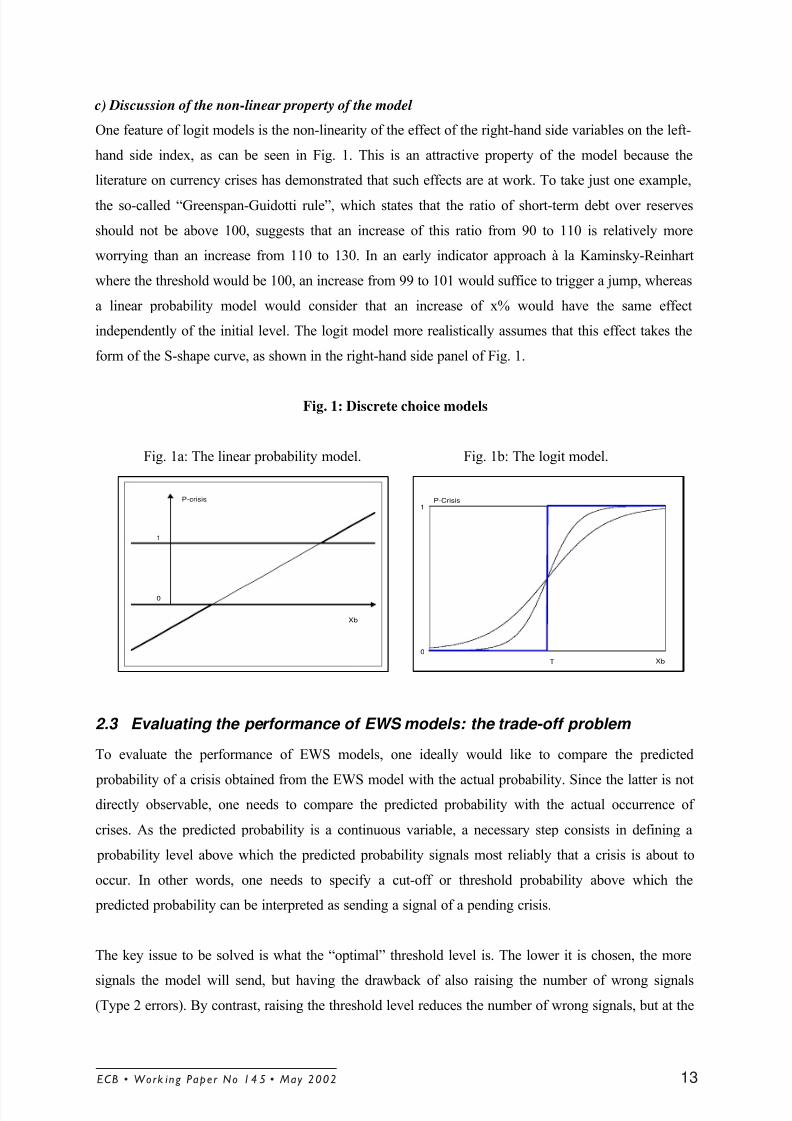
c) Discussion of the non-linear property of the model
One feature of logit models is the non-linearity of the effect of the right-hand side variables on the left-
hand side index, as can be seen in Fig. 1. This is an attractive property of the model because the
literature on currency crises has demonstrated that such effects are at work. To take just one example,
the so-called “Greenspan-Guidotti rule”, which states that the ratio of short-term debt over reserves
should not be above 100, suggests that an increase of this ratio from 90 to 110 is relatively more
worrying than an increase from 110 to 130. In an early indicator approach à la Kaminsky-Reinhart
where the threshold would be 100, an increase from 99 to 101 would suffice to trigger a jump, whereas
a linear probability model would consider that an increase of x% would have the same effect
independently of the initial level. The logit model more realistically assumes that this effect takes the
form of the S-shape curve, as shown in the right-hand side panel of Fig. 1.
Fig. 1: Discrete choice models
Fig. 1a: The linear probability model. Fig. 1b: The logit model.
2.3 Evaluating the performance of EWS models: the trade-off problem
To evaluate the performance of EWS models, one ideally would like to compare the predicted
probability of a crisis obtained from the EWS model with the actual probability. Since the latter is notdirectly observable, one needs to compare the predicted probability with the actual occurrence of
crises. As the predicted probability is a continuous variable, a necessary step consists in defining a
probability level above which the predicted probability signals most reliably that a crisis is about to
occur. In other words, one needs to specify a cut-off or threshold probability above which the
predicted probability can be interpreted as sending a signal of a pending crisis.
The key issue to be solved is what the “optimal” threshold level is. The lower it is chosen, the more
signals the model will send, but having the drawback of also raising the number of wrong signals
(Type 2 errors). By contrast, raising the threshold level reduces the number of wrong signals, but at the
P-crisis
Xb
1
0
0
1
XbT
P-Crisis
ECB • Work ing Paper No 14 5 • May 2002 13
8/3/2019 Early Warning System Europe
http://slidepdf.com/reader/full/early-warning-system-europe 15/67
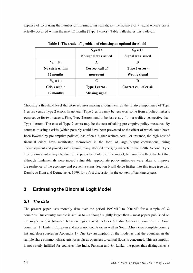
expense of increasing the number of missing crisis signals, i.e. the absence of a signal when a crisis
actually occurred within the next 12 months (Type 1 errors). Table 1 illustrates this trade-off.
Table 1: The trade-off problem of choosing an optimal threshold
Si,t = 0 :
No signal was issued
Si,t = 1 :
Signal was issued
Yi,t = 0 :
No crisis within
12 months
A
Correct call of
non-event
B
Type 2 error -
Wrong signal
Yi,t = 1 :
Crisis within
12 months
C
Type 1 error -
Missing signal
D
Correct call of crisis
Choosing a threshold level therefore requires making a judgement on the relative importance of Type
1 errors versus Type 2 errors. In general, Type 2 errors may be less worrisome from a policy-maker’s
perspective for two reasons. First, Type 2 errors tend to be less costly from a welfare perspective than
Type 1 errors. The cost of Type 2 errors may be the cost of taking pre-emptive policy measures. By
contrast, missing a crisis (which possibly could have been prevented or the effect of which could have
been lowered by pre-emptive policies) has often a higher welfare cost. For instance, the high cost of
financial crises have manifested themselves in the form of large output contractions, risingunemployment and poverty rates among many affected emerging markets in the 1990s. Second, Type
2 errors may not always be due to the predictive failure of the model, but simply reflect the fact that
although fundamentals were indeed vulnerable, appropriate policy initiatives were taken to improve
the resilience of the economy and prevent a crisis. Section 6 will delve further into this issue (see also
Demirguc-Kunt and Detragiache, 1999, for a first discussion in the context of banking crises).
3 Estimating the Binomial Logit Model
3.1 The data
The present paper uses monthly data over the period 1993M12 to 2001M9 for a sample of 32
countries. Our country sample is similar to – although slightly larger than – most papers published on
the subject and is balanced between regions as it includes 8 Latin American countries, 12 Asian
countries, 11 Eastern European and accession countries, as well as South Africa (see complete country
list and data sources in Appendix 1). One key assumption of the model is that the countries in the
sample share common characteristics as far as openness to capital flows is concerned. This assumption
is not strictly fulfilled for countries like India, Pakistan and Sri Lanka; the paper thus distinguishes a
ECB • Work in g Paper No 145 • May 200214
8/3/2019 Early Warning System Europe
http://slidepdf.com/reader/full/early-warning-system-europe 16/67
sub-group of 20 “core countries”, which analyses only the most open emerging markets and also
corresponds to the two IMF models most directly related to the present study. Although results are not
dramatically different between the full and the core country samples of our data set in terms of which
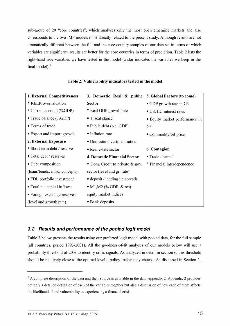
variables are significant, results are better for the core countries in terms of prediction. Table 2 lists the
right-hand side variables we have tested in the model (a star indicates the variables we keep in the
final model).5
Table 2: Vulnerability indicators tested in the model
1. External Competitiveness
* REER overvaluation
* Current account (%GDP)
• Trade balance (%GDP)
• Terms of trade
• Export and import growth
2. External Exposure
* Short-term debt / reserves
• Total debt / reserves
• Debt composition
(loans/bonds, misc. concepts).
• FDI, portfolio investment
• Total net capital inflows
• Foreign exchange reserves
(level and growth rate).
3. Domestic Real & public
Sector
* Real GDP growth rate
• Fiscal stance
• Public debt (p.c. GDP)
• Inflation rate
• Domestic investment ratios
• Real estate sector
4. Domestic Financial Sector
* Dom. Credit to private & gov.
sector (level and gr. rate)
• deposit / lending i.r. spreads
• M1,M2 (% GDP, & res).
equity market indices
• Bank deposits
5. Global Factors (to come)
• GDP growth rate in G3
• US, EU interest rates
• Equity market performance in
G3
• Commodity/oil price
6. Contagion
• Trade channel
* Financial interdependence
3.2 Results and performance of the pooled logit model
Table 3 below presents the results using our preferred logit model with pooled data, for the full sample
(all countries, period 1993-2001). All the goodness-of-fit analyses of our models below will use a
probability threshold of 20% to identify crisis signals. As analyzed in detail in section 6, this threshold
should be relatively close to the optimal level a policy-maker may choose. As discussed in Section 2,
5A complete description of the data and their source is available in the data Appendix 2. Appendix 2 provides
not only a detailed definition of each of the variables together but also a discussion of how each of them affects
the likelihood of and vulnerability to experiencing a financial crisis.
ECB • Work ing Paper No 14 5 • May 2002 15
8/3/2019 Early Warning System Europe
http://slidepdf.com/reader/full/early-warning-system-europe 17/67
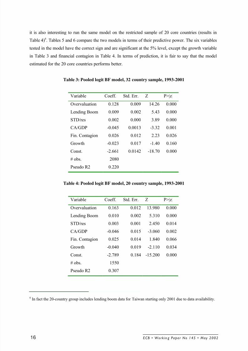
it is also interesting to run the same model on the restricted sample of 20 core countries (results in
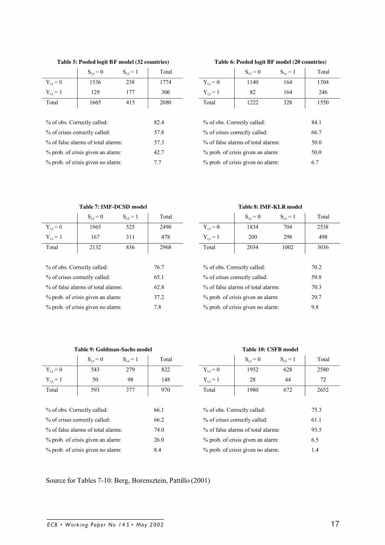
Table 4)6. Tables 5 and 6 compare the two models in terms of their predictive power. The six variables
tested in the model have the correct sign and are significant at the 5% level, except the growth variable
in Table 3 and financial contagion in Table 4. In terms of prediction, it is fair to say that the model
estimated for the 20 core countries performs better.
Table 3: Pooled logit BF model, 32 country sample, 1993-2001
Variable Coeff. Std. Err. Z P>|z|
Overvaluation 0.128 0.009 14.26 0.000
Lending Boom 0.009 0.002 5.43 0.000
STD/res 0.002 0.000 3.89 0.000
CA/GDP -0.045 0.0013 -3.32 0.001
Fin. Contagion 0.026 0.012 2.23 0.026
Growth -0.023 0.017 -1.40 0.160
Const. -2.661 0.0142 -18.70 0.000
# obs. 2080
Pseudo R2 0.220
Table 4: Pooled logit BF model, 20 country sample, 1993-2001
Variable Coeff. Std. Err. Z P>|z|
Overvaluation 0.163 0.012 13.980 0.000
Lending Boom 0.010 0.002 5.310 0.000
STD/res 0.003 0.001 2.450 0.014
CA/GDP -0.046 0.015 -3.060 0.002
Fin. Contagion 0.025 0.014 1.840 0.066
Growth -0.040 0.019 -2.110 0.034
Const. -2.789 0.184 -15.200 0.000
# obs. 1550
Pseudo R2 0.307
6In fact the 20-country group includes lending boom data for Taiwan starting only 2001 due to data availability.
ECB • Work in g Paper No 145 • May 200216
8/3/2019 Early Warning System Europe
http://slidepdf.com/reader/full/early-warning-system-europe 18/67
Table 5: Pooled logit BF model (32 countries)
Si,t = 0 Si,t = 1 Total
Yi,t = 0 1536 238 1774
Yi,t
= 1 129 177 306
Total 1665 415 2080
% of obs. Correctly called: 82.4
% of crises correctly called: 57.8
% of false alarms of total alarms: 57.3
% prob. of crisis given an alarm: 42.7
% prob. of crisis given no alarm: 7.7
Table 6: Pooled logit BF model (20 countries)
Si,t = 0 Si,t = 1 Total
Yi,t = 0 1140 164 1304
Yi,t
= 1 82 164 246
Total 1222 328 1550
% of obs. Correctly called: 84.1
% of crises correctly called: 66.7
% of false alarms of total alarms: 50.0
% prob. of crisis given an alarm: 50.0
% prob. of crisis given no alarm: 6.7
Table 7: IMF-DCSD model
Si,t = 0 Si,t = 1 Total
Yi,t = 0 1965 525 2490
Yi,t = 1 167 311 478
Total 2132 836 2968
% of obs. Correctly called: 76.7
% of crises correctly called: 65.1
% of false alarms of total alarms: 62.8
% prob. of crisis given an alarm: 37.2
% prob. of crisis given no alarm: 7.8
Table 8: IMF-KLR model
Si,t = 0 Si,t = 1 Total
Yi,t = 0 1834 704 2538
Yi,t = 1 200 298 498
Total 2034 1002 3036
% of obs. Correctly called: 70.2
% of crises correctly called: 59.8
% of false alarms of total alarms: 70.3
% prob. of crisis given an alarm: 29.7
% prob. of crisis given no alarm: 9.8
Table 9: Goldman-Sachs model
Si,t = 0 Si,t = 1 Total
Yi,t = 0 543 279 822
Yi,t = 1 50 98 148Total 593 377 970
% of obs. Correctly called: 66.1
% of crises correctly called: 66.2
% of false alarms of total alarms: 74.0
% prob. of crisis given an alarm: 26.0
% prob. of crisis given no alarm: 8.4
Table 10: CSFB model
Si,t = 0 Si,t = 1 Total
Yi,t = 0 1952 628 2580
Yi,t = 1 28 44 72Total 1980 672 2652
% of obs. Correctly called: 75.3
% of crises correctly called: 61.1
% of false alarms of total alarms: 93.5
% prob. of crisis given an alarm: 6.5
% prob. of crisis given no alarm: 1.4
Source for Tables 7-10: Berg, Borensztein, Pattillo (2001)
ECB • Work ing Paper No 14 5 • May 2002 17
8/3/2019 Early Warning System Europe
http://slidepdf.com/reader/full/early-warning-system-europe 19/67
The main point to note is that, with a similar methodology as many other papers published on the
subject, the present model performs already better in terms of prediction. Tables 5 to 10 allow a
comparison of the goodness-of-fit of our pooled model with those models of previous studies on the
subject.
Our model for 20 countries (Table 6) performs better in each of the five goodness-of-fit criteria than
the IMF-DCSD model (Table 7), the Kaminsky-Lizondo-Reinhart model (Table 8) as well as the
private sector models by Goldman-Sachs (Table 9) and Credit Suisse First Boston (Table 10).7
Our
model correctly calls the highest ratio of observations (84.1%) and of crises months (66.7%), and it
gives the fewest false signals of any of the models. The conditional probability of having a crisis if an
alarm occurred is 50%, which is much higher than any of the other models. This number may not seem
high, but it is still reasonably good when comparing it to the unconditional probability of experiencing
a crisis, which is in our model 15.8% (i.e. 246 months out of a total of 1550 months were months for
which a crisis followed within the subsequent 12 months). The better performance of our pooled
model using the same methodology as most of these models means that the variables we have been
using are more reliable, and/or that the country sample and time period has been more appropriate.
3.3 Panel data analysis
One potential drawback of the model with pooled data is that it ignores some available information,
namely the cross-sectional and time series dimensions of the data. It could be the case that some
important information on a particular country is omitted from the pooled model. For example, the
capital account of a given country may not be as open as that of other countries, which would induce
the model to overestimate the probability of a crisis. Conversely, the political situation of a country
could be such that we permanently underestimate this probability. Fixed and random effects are useful
tools to approach these issues. In the literature on panel data it is common to distinguish between the
“between” information (comparing across countries) and the “within” information (comparing the
evolution of the variables with the country specific mean, ignoring inter-country comparison). Fixedeffects are equivalent to country dummies: they focus on the within information only. As such, they
constitute a loss of information, but the estimates are unbiased. Random effects are more efficient
because they do not consider country effects as fixed but as random and combine more efficiently the
between and the within information. However, they are potentially biased: random effects assume that
7The KLR model uses an indicator approach, as discussed in section 2.2.1, with a 2-year forecast horizon. The
Goldman-Sachs and the CSFB models also use a logit methodology, although they partly have a longer sample
period but fewer countries and different forecast horizons (3 months for the GS model, 1 month for the CSFB
model)
ECB • Work in g Paper No 145 • May 200218
8/3/2019 Early Warning System Europe
http://slidepdf.com/reader/full/early-warning-system-europe 20/67
individual specific effects are uncorrelated with the independent variables, which may not be the case
in our context (for instance, if individual effects arise because of the political setting of a given
country, macroeconomic variables are likely to be also affected by the political situation). Table 22 in
Appendix 3 reports the goodness of fit results for the random effect model, which faired better than
using fixed effects. Still, the improvement is not very clear and the tests we have conducted deterred
us from using fixed or random effects. An additional consideration was that with fixed effects non-
crisis countries are excluded from the sample, which may induce a sample bias.8
4 A Multinomial Logit EWS Approach
4.1 Explaining the post-crisis bias
What we call the “post-crisis bias” is an important econometric problem that so far, to our knowledge,
has not been addressed in the empirical literature on currency crisis models. The “post-crisis bias”
implies that the econometric results of models that try to explain or predict crises can at least in part,
or even fully be explained by the behavior of the independent variables during and directly after a
crisis. Recall that an EWS model aims to analyze how vulnerable to a crisis the situation in a country
is. The correct way of doing this is by comparing the behavior of the independent variables before a
crisis with their behavior during periods when these variables are sustainable, i.e. during tranquil or
“normal” times. Instead, what EWS models with two outcomes do is comparing the pre-crisis
observations with the observations both during tranquil periods and post-crisis/recovery periods. This
can lead to an important bias because the behavior of the independent variables is very different during
tranquil times as compared to recovery episodes.
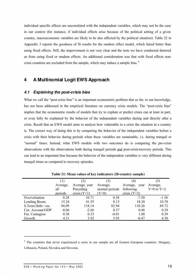
Table 11: Mean values of key indicators (20-country sample)
(1)Average,all
periods
(2)Average, year Preceding
crisis (Y=1)
(3)Average,normal periods
(Y=0)
(4)Average, year following
crisis (Y=2)
(5)Average,Y=0 or Y=2.
Overvaluation 0.28 10.71 0.38 -7.50 -1.56Lending Boom 15.24 41.55 8.15 18.38 10.70S.Term Debt / res. 94.09 118.14 82.94 110.26 89.72Cur. Account/GDP -0.06 -2.66 0.37 0.46 0.39Fin. Contagion 0.38 0.33 -0.01 1.88 0.39Growth 4.31 3.92 5.95 -0.47 4.38
8
The countries that never experienced a crisis in our sample are all Eastern European countries: Hungary,
Lithuania, Poland, Slovakia and Slovenia.
ECB • Work ing Paper No 14 5 • May 2002 19
8/3/2019 Early Warning System Europe
http://slidepdf.com/reader/full/early-warning-system-europe 21/67
Table 11 provides further evidence for this bias for six key leading indicators used in our benchmark
model below. Recall that what an EWS model aims to test is whether we can extract information from
economic variables about the sustainability and the probability of a looming currency crisis by
comparing their behavior during tranquil or “normal” times as compared to pre-crisis periods. The
relevant comparison therefore is between column (2), which shows the means of these indicators in the
pre-crisis period, and column (3), which corresponds to what we define as “normal periods”.
By contrast, what traditional two-state logit or probit models do is estimate the link between the pre-
crisis period of column (2) with the combined tranquil and post-crisis episodes shown in column (5).
As column (4) reveals, crisis and post-crisis/recovery periods are often disorderly and volatile
corrections towards longer-term equilibria. They should not be included in an analysis of anticipating
crises because one can not extract meaningful information about the sustainability and vulnerability of
a country’s economic fundamentals by looking at crisis and post-crisis observations.
Further evidence for the post-crisis bias is provided by the event analysis in Appendix 5 for a set of 28
independent variables. The advantage of the event analysis is that it nicely illustrates the dynamics of
the adjustment process of the independent variables before and after a crisis. Period t in the charts
indicates the onset of a currency crisis. The thick line indicates the behavior of each variable from 12
months before till 12 months after the onset of the crisis. This thick line is calculated as the mean of
the variable over all currency crises in our sample. The thinner, horizontal line indicates the mean of
each variable during tranquil periods. The charts confirm that the behavior of most independent
variables is substantially different in pre-crisis times from recovery episodes. Equally important is that
most variables are substantially different in tranquil periods compared to recovery times.
Not distinguishing between tranquil and recovery periods may therefore introduce an important bias in
an EWS model. Section 4.2 discusses ways of solving this bias, whereas section 5 will show that the
bias is indeed important, and that solving it improves the predictive power of the EWS substantially.
4.2 How to address the post-crisis bias
There are at least two ways of tackling the post-crisis bias. The first, crudest way would be to drop out
all post-crisis observations from the data and then to estimate the standard two outcome discrete-
dependent-variable model, as done for example in Demirguc-Kunt and Detragiache (1998).9
The
drawback of such a method is that it ignores data that potentially could provide valuable information,
9
The paper by Demirguc-Kunt and Detragiache (1998) is otherwise very distinct from ours in that it looks at a
different type of crisis (banking crises) and in particular some specific events.
ECB • Work in g Paper No 145 • May 200220
8/3/2019 Early Warning System Europe
http://slidepdf.com/reader/full/early-warning-system-europe 22/67
for instance on how the economic variables behave during recoveries and when or whether economic
variables return to levels of tranquil or “normal” times. A second and our preferred alternative is a
discrete-dependent-variable approach with more than two outcomes, in our case a multinomial logit
model. For the case of the EWS model, we construct a multinomial logit model with three outcomes:
ïî
ïí
ì
==∃
==∃
= −
+
otherwise
CC t sk if
CC t sk if
Y i
k t
i
k t
i
t
0
,1..12...12
,1..12...11
(10)
i.e. a pre-crisis regime for the 12 months prior to the onset of a crisis (Yi,t = 1), a post-crisis/recovery
regime for the crisis itself and 12 months following the end of the crisis (Y i,,t = 2), and a tranquil
regime for all other times (Yi,,t = 0). Let us delve further into these definitions. The regime that
corresponds to Y=1 announces a crisis in the next 12 months. Forwarding the left-hand side variable
and using it on contemporaneous right-hand side variables allows a considerable simplification of the
notation: otherwise we would need to include in the right-hand side all 12 lags of the six variables, i.e.
72 variables. Above all, it directly follows from the approach outlined in the definition: the present
paper does not try to predict the timing of a crisis exactly k months ahead, which would be the
outcome of a model in which right-hand side variables show up at lag k. Instead, the model tells us
whether a crisis can happen any time in the following 12 months. The fact that the left-hand side
variable is a forward variable ensures that the same variables (the exchange rate and the level of
reserves) never simultaneously appear on both sides of the equation: the statement yielded by the
model is that a low level of reserves (compared to debt) and an overvalued exchange rate now are
likely to trigger a further drop in reserves and/or a devaluation of the exchange rate later .
The definition of the regime corresponding to Y=2 follows a similar logic. Once a country has
experienced a crisis, it will take some time before it recovers. This time can considerably vary from
one country to the next. In parallel with the definition of regime 1 announcing a crisis, regime 2
announces a recovery. We based our definition of regime 2, again, on the EMP, as Fig. 1.c below
exemplifies. This figure represents the EMP of two fictitious countries that underwent a crisis at the
same time, T. Consequently, their discrete crisis indices coincide in the pre-crisis period for which
Y=1. However, the post-crisis/recovery period varies for these two countries. For country A the crisis
is relatively short and the EMP returns to “normal” (i.e. a mean slightly below zero and low variance)
relatively quickly. For country B the crisis is deeper and more protracted; recovery is then longer than
for country A. As a consequence the period for which Y=2 is longer for country B than for country A.
To date the end of regime 2, we used a strong empirical observation for the countries included in the
sample: the return to normal generally occurred 12 months after the last observation for which the
ECB • Work ing Paper No 14 5 • May 2002 21
8/3/2019 Early Warning System Europe
http://slidepdf.com/reader/full/early-warning-system-europe 23/67
EMP index was above the critical threshold. It is this observation that led us to define outcome 2 as of
equation (10)10
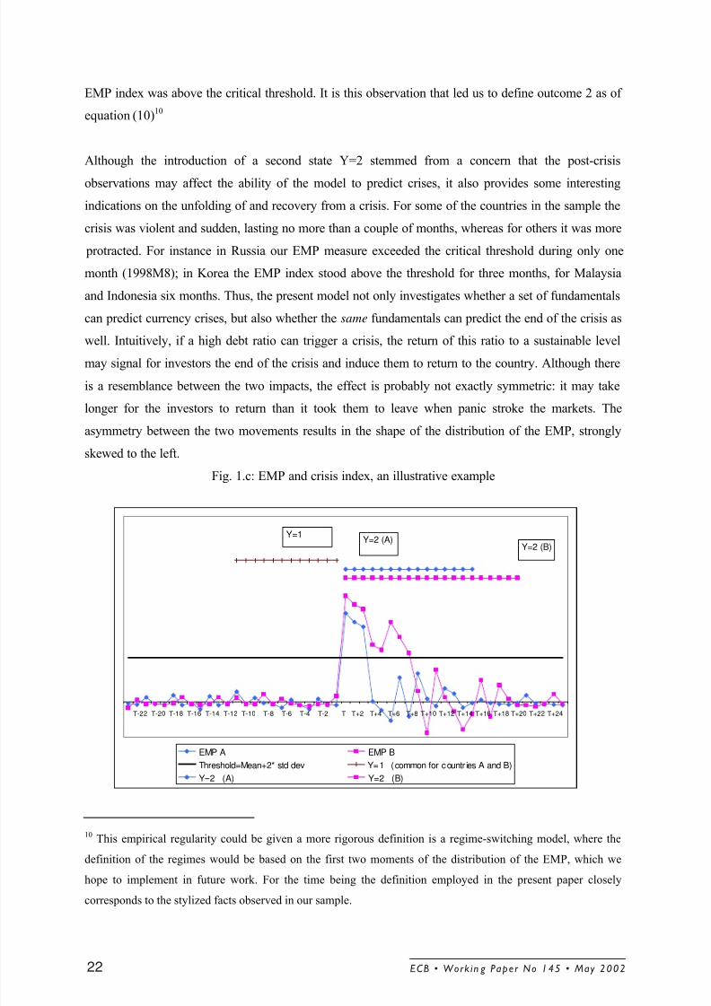
Although the introduction of a second state Y=2 stemmed from a concern that the post-crisis
observations may affect the ability of the model to predict crises, it also provides some interesting
indications on the unfolding of and recovery from a crisis. For some of the countries in the sample the
crisis was violent and sudden, lasting no more than a couple of months, whereas for others it was more
protracted. For instance in Russia our EMP measure exceeded the critical threshold during only one
month (1998M8); in Korea the EMP index stood above the threshold for three months, for Malaysia
and Indonesia six months. Thus, the present model not only investigates whether a set of fundamentals
can predict currency crises, but also whether the same fundamentals can predict the end of the crisis as
well. Intuitively, if a high debt ratio can trigger a crisis, the return of this ratio to a sustainable level
may signal for investors the end of the crisis and induce them to return to the country. Although there
is a resemblance between the two impacts, the effect is probably not exactly symmetric: it may take
longer for the investors to return than it took them to leave when panic stroke the markets. The
asymmetry between the two movements results in the shape of the distribution of the EMP, strongly
skewed to the left.
Fig. 1.c: EMP and crisis index, an illustrative example
10This empirical regularity could be given a more rigorous definition is a regime-switching model, where the
definition of the regimes would be based on the first two moments of the distribution of the EMP, which we
hope to implement in future work. For the time being the definition employed in the present paper closely
corresponds to the stylized facts observed in our sample.
T-22 T-20 T-18 T-16 T-14 T-12 T-10 T-8 T-6 T-4 T-2 T T+2 T+4 T+6 T+8 T+10 T+12 T+14 T+16 T+18 T+20 T+22 T+24
EMP A EMP B
Threshold=Mean+2* std dev Y=1 (common for countr ies A and B)
Y=2 (A) Y=2 (B)
Y=1Y=2 (A)
Y=2 (B)
ECB • Work in g Paper No 145 • May 200222
8/3/2019 Early Warning System Europe
http://slidepdf.com/reader/full/early-warning-system-europe 24/67
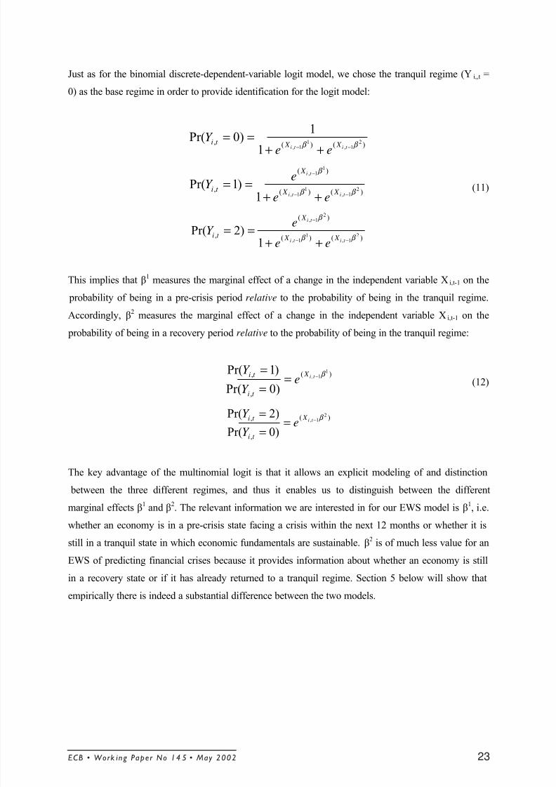
Just as for the binomial discrete-dependent-variable logit model, we chose the tranquil regime (Yi,,t =
0) as the base regime in order to provide identification for the logit model:
)()(, 21,
11,1
1)0Pr( β β −− ++== t it i X X t i
eeY
)()(
)(
, 21,
11,
11,
1)1Pr(
β β
β
−−
−
++==
t it i
t i
X X
X
t i
ee
eY (11)
)()(
)(
, 21,
11,
21,
1)2Pr(
β β
β
−−
−
++==
t it i
t i
X X
X
t i
ee
eY
This implies that β1 measures the marginal effect of a change in the independent variable Xi,t-1 on the
probability of being in a pre-crisis period relative to the probability of being in the tranquil regime.
Accordingly, β2
measures the marginal effect of a change in the independent variable Xi,t-1 on the
probability of being in a recovery period relative to the probability of being in the tranquil regime:
)(
,
,1
1,
)0Pr(
)1Pr( β −==
=t i X
t i
t ie
Y
Y (12)
)(
,
,2
1,
)0Pr()2Pr( β −=
== t i X
t i
t ie
Y Y
The key advantage of the multinomial logit is that it allows an explicit modeling of and distinction
between the three different regimes, and thus it enables us to distinguish between the different
marginal effects β1
and β2. The relevant information we are interested in for our EWS model is β
1, i.e.
whether an economy is in a pre-crisis state facing a crisis within the next 12 months or whether it is
still in a tranquil state in which economic fundamentals are sustainable. β2
is of much less value for an
EWS of predicting financial crises because it provides information about whether an economy is still
in a recovery state or if it has already returned to a tranquil regime. Section 5 below will show that
empirically there is indeed a substantial difference between the two models.
ECB • Work ing Paper No 14 5 • May 2002 23
8/3/2019 Early Warning System Europe
http://slidepdf.com/reader/full/early-warning-system-europe 25/67
5 Multinomial Logit EWS Model: Results and Robustness Tests
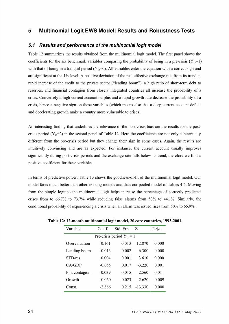
5.1 Results and performance of the multinomial logit model
Table 12 summarizes the results obtained from the multinomial logit model. The first panel shows the
coefficients for the six benchmark variables comparing the probability of being in a pre-crisis (Yi,t=1)
with that of being in a tranquil period (Yi,t=0). All variables enter the equation with a correct sign and
are significant at the 1% level. A positive deviation of the real effective exchange rate from its trend, a
rapid increase of the credit to the private sector (“lending boom”), a high ratio of short-term debt to
reserves, and financial contagion from closely integrated countries all increase the probability of a
crisis. Conversely a high current account surplus and a rapid growth rate decrease the probability of a
crisis, hence a negative sign on these variables (which means also that a deep current account deficit
and decelerating growth make a country more vulnerable to crises).
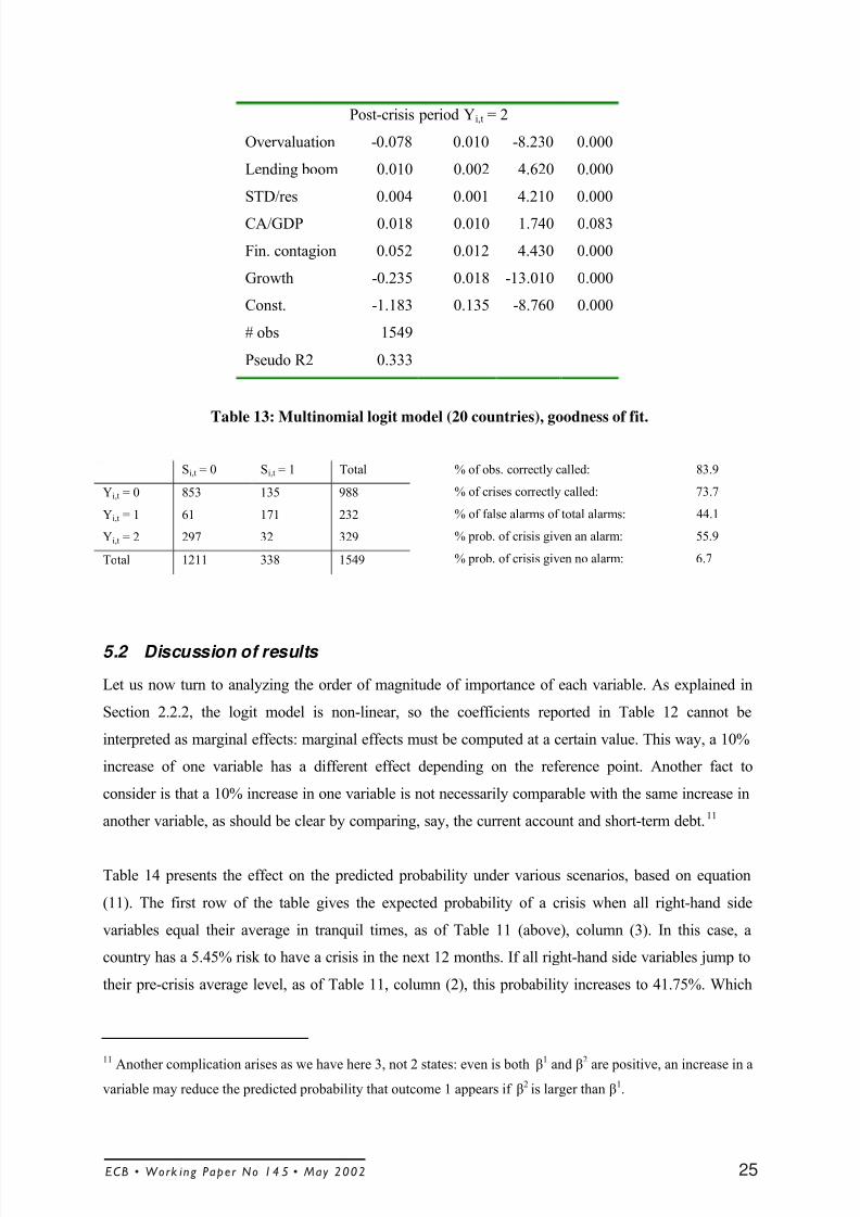
An interesting finding that underlines the relevance of the post-crisis bias are the results for the post-
crisis period (Yi,t=2) in the second panel of Table 12. Here the coefficients are not only substantially
different from the pre-crisis period but they change their sign in some cases. Again, the results are
intuitively convincing and are as expected. For instance, the current account usually improves
significantly during post-crisis periods and the exchange rate falls below its trend, therefore we find a
positive coefficient for these variables.
In terms of predictive power, Table 13 shows the goodness-of-fit of the multinomial logit model. Our
model fares much better than other existing models and than our pooled model of Tables 4-5. Moving
from the simple logit to the multinomial logit helps increase the percentage of correctly predicted
crises from to 66.7% to 73.7% while reducing false alarms from 50% to 44.1%. Similarly, the
conditional probability of experiencing a crisis when an alarm was issued rises from 50% to 55.9%.
Table 12: 12-month multinomial logit model, 20 core countries, 1993-2001.
Variable Coeff. Std. Err. Z P>|z|
Pre-crisis period Yi,t = 1
Overvaluation 0.161 0.013 12.870 0.000
Lending boom 0.013 0.002 6.300 0.000
STD/res 0.004 0.001 3.610 0.000
CA/GDP -0.055 0.017 -3.220 0.001
Fin. contagion 0.039 0.015 2.560 0.011
Growth -0.060 0.023 -2.620 0.009
Const. -2.866 0.215 -13.330 0.000
ECB • Work in g Paper No 145 • May 200224
8/3/2019 Early Warning System Europe
http://slidepdf.com/reader/full/early-warning-system-europe 26/67
Post-crisis period Yi,t = 2
Overvaluation -0.078 0.010 -8.230 0.000
Lending boom 0.010 0.002 4.620 0.000
STD/res 0.004 0.001 4.210 0.000
CA/GDP 0.018 0.010 1.740 0.083
Fin. contagion 0.052 0.012 4.430 0.000
Growth -0.235 0.018 -13.010 0.000
Const. -1.183 0.135 -8.760 0.000
# obs 1549
Pseudo R2 0.333
Table 13: Multinomial logit model (20 countries), goodness of fit.
Si,t = 0 Si,t = 1 Total
Yi,t = 0 853 135 988
Yi,t = 1 61 171 232
Yi,t = 2 297 32 329
Total 1211 338 1549
% of obs. correctly called: 83.9
% of crises correctly called: 73.7
% of false alarms of total alarms: 44.1
% prob. of crisis given an alarm: 55.9
% prob. of crisis given no alarm: 6.7
5.2 Discussion of results
Let us now turn to analyzing the order of magnitude of importance of each variable. As explained in
Section 2.2.2, the logit model is non-linear, so the coefficients reported in Table 12 cannot be
interpreted as marginal effects: marginal effects must be computed at a certain value. This way, a 10%
increase of one variable has a different effect depending on the reference point. Another fact to
consider is that a 10% increase in one variable is not necessarily comparable with the same increase in
another variable, as should be clear by comparing, say, the current account and short-term debt.11
Table 14 presents the effect on the predicted probability under various scenarios, based on equation
(11). The first row of the table gives the expected probability of a crisis when all right-hand side
variables equal their average in tranquil times, as of Table 11 (above), column (3). In this case, a
country has a 5.45% risk to have a crisis in the next 12 months. If all right-hand side variables jump to
their pre-crisis average level, as of Table 11, column (2), this probability increases to 41.75%. Which
11
Another complication arises as we have here 3, not 2 states: even is both β1
and β2
are positive, an increase in a
variable may reduce the predicted probability that outcome 1 appears if β2
is larger than β1.
ECB • Work ing Paper No 14 5 • May 2002 25
8/3/2019 Early Warning System Europe
http://slidepdf.com/reader/full/early-warning-system-europe 27/67
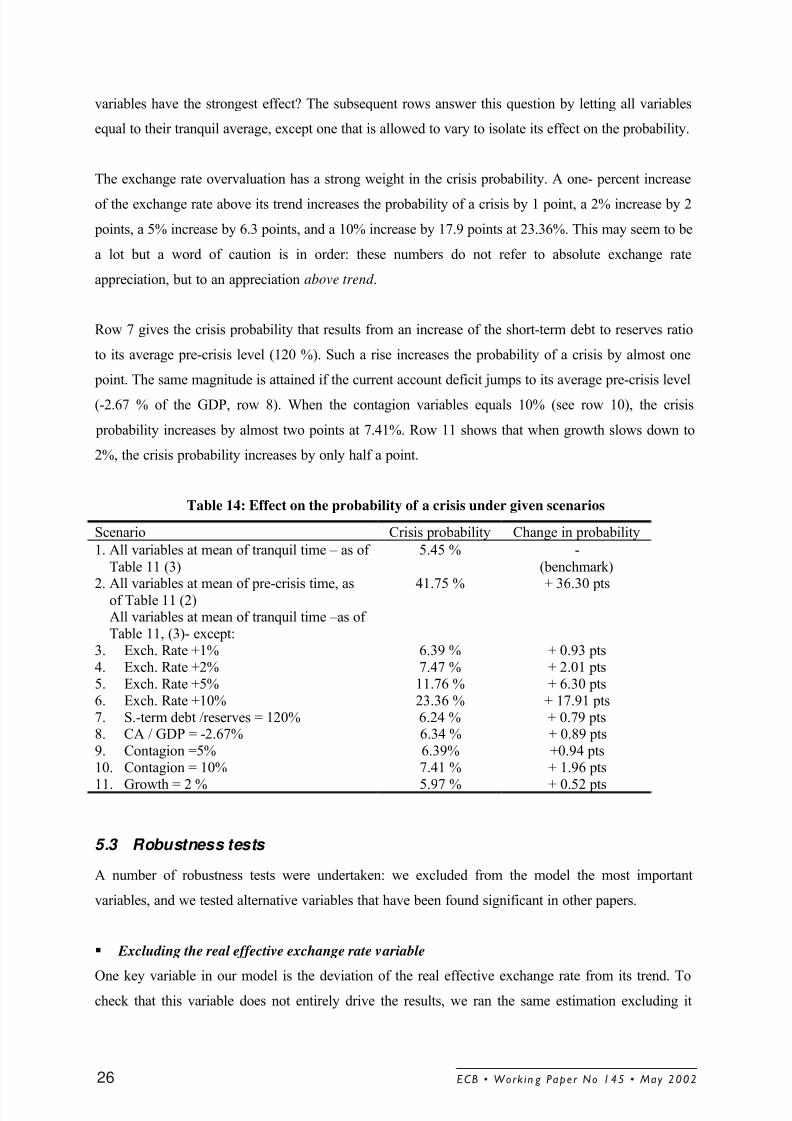
variables have the strongest effect? The subsequent rows answer this question by letting all variables
equal to their tranquil average, except one that is allowed to vary to isolate its effect on the probability.
The exchange rate overvaluation has a strong weight in the crisis probability. A one- percent increase
of the exchange rate above its trend increases the probability of a crisis by 1 point, a 2% increase by 2
points, a 5% increase by 6.3 points, and a 10% increase by 17.9 points at 23.36%. This may seem to be
a lot but a word of caution is in order: these numbers do not refer to absolute exchange rate
appreciation, but to an appreciation above trend .
Row 7 gives the crisis probability that results from an increase of the short-term debt to reserves ratio
to its average pre-crisis level (120 %). Such a rise increases the probability of a crisis by almost one
point. The same magnitude is attained if the current account deficit jumps to its average pre-crisis level
(-2.67 % of the GDP, row 8). When the contagion variables equals 10% (see row 10), the crisis
probability increases by almost two points at 7.41%. Row 11 shows that when growth slows down to
2%, the crisis probability increases by only half a point.
Table 14: Effect on the probability of a crisis under given scenarios
Scenario Crisis probability Change in probability
1. All variables at mean of tranquil time – as of
Table 11 (3)
5.45 % -
(benchmark)
2. All variables at mean of pre-crisis time, asof Table 11 (2) 41.75 % + 36.30 pts
All variables at mean of tranquil time –as of Table 11, (3)- except:
3. Exch. Rate +1% 6.39 % + 0.93 pts4. Exch. Rate +2% 7.47 % + 2.01 pts5. Exch. Rate +5% 11.76 % + 6.30 pts6. Exch. Rate +10% 23.36 % + 17.91 pts7. S.-term debt /reserves = 120% 6.24 % + 0.79 pts8. CA / GDP = -2.67% 6.34 % + 0.89 pts9. Contagion =5% 6.39% +0.94 pts10. Contagion = 10% 7.41 % + 1.96 pts
11. Growth = 2 % 5.97 % + 0.52 pts
5.3 Robustness tests
A number of robustness tests were undertaken: we excluded from the model the most important
variables, and we tested alternative variables that have been found significant in other papers.
§ Excluding the real effective exchange rate variable
One key variable in our model is the deviation of the real effective exchange rate from its trend. Tocheck that this variable does not entirely drive the results, we ran the same estimation excluding it
ECB • Work in g Paper No 145 • May 200226
8/3/2019 Early Warning System Europe
http://slidepdf.com/reader/full/early-warning-system-europe 28/67
8/3/2019 Early Warning System Europe
http://slidepdf.com/reader/full/early-warning-system-europe 29/67
• Short-term debt over GDP
To check that the short-term debt to reserves ratio is not significant simply because the denominator
diminishes before a crisis, we tested the level of short-term debt measured as a percentage of GDP.
The result is conclusive: this variable is significant and contributes to the predictions in an important
way as well. Both in view of the importance of the Greenspan-Guidotti rule and to avoid potential
multicollinearity with the current account (if both are scaled with GDP), we decided to scale short-
term debt with reserves.
• Current account items
The present model uses the current account over GDP ratio. As the trade balance would be an obvious
alternative, we tested it, separately and together with the current account. When the trade balance is
included alone it is significant with the correct sign; when it is tested together with the current account
it is no longer significant, from which we conclude that the current account is a preferable indicator,
probably because it incorporates more information. Interestingly, the growth rate of exports has the
expected negative sign and helps predict slightly more crises. Openness of the country, measured as
the sum of imports and exports over GDP, is not significant: more open countries do not expose
themselves to a higher risk.
• FDI and portfolio investment It has sometimes been argued that the size and the nature of capital flows matters for currency crises,
in particular, there is a general perception that FDI is a better investment than portfolio investment for
the domestic economy. To investigate this issue, we included in the equation FDI and portfolio
investment, both as a level of the net value (expressed in percent of GDP) and as a growth rate. As can
be seen on Table 16d, the variables on the levels did not enter the specification significantly. On the
other hand, it is interesting to note that the growth rate of FDI inflows comes close to the 10%
threshold: it seems that an increase in FDI inflows has some effect in avoiding currency crises.
To summarize, in order to keep the model tractable and as simple as possible we limited ourselves to a
relatively small number of variables. However, other variables may be included in an extended model
and are certainly worth monitoring in an extended model: the growth rate of reserves, both as a level
and as a percentage of exports, the market index of domestic banks, and the growth rate of FDI
inflows.
ECB • Work in g Paper No 145 • May 200228
8/3/2019 Early Warning System Europe
http://slidepdf.com/reader/full/early-warning-system-europe 30/67
5.4 Out-of-sample performance
Since the important contribution of Berg and Pattillo (1998) on the frequent failure of models to
predict crises in subsequent episodes, out-of-sample forecasts have become the corner-stone of testing
the goodness-of-fit of EWS models. Indeed, in-sample properties do not ensure that the model can
predict future crises if the causes of currency crises drastically vary from one episode to the next. To
check that our model is also able to predict crises out-of-sample, we estimate the model on restricted
periods and computed the probability of a crisis in the following 12 months.
We conduct the out-of-sample test for three episodes: for the Asian crisis of 1997, for various
emerging market crises in 1998 (including Russia and Brazil), and for the recent crises in Turkey and
Argentina in 2001. Note that the out-of-sample models include the same six key variables from our
benchmark model above. This is not strictly “out-of-sample” as some included variables may not besignificant for the shorter out-of-sample models whereas other, excluded variables may have been
significant for the shorter out-of-sample model periods. The reason for restricting the model to the six
key variables is to obtain a comparison between the in-sample and the out-of-sample performance of
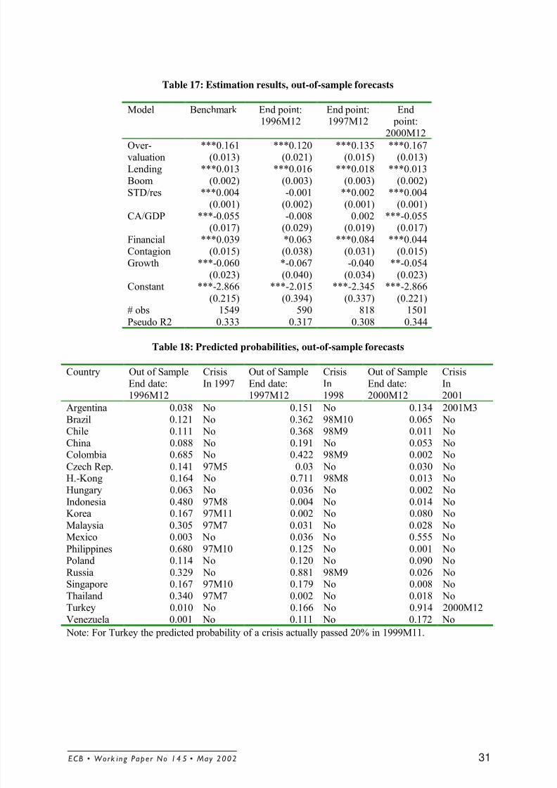
our benchmark model. Table 17 shows the estimation results for the various sub-samples that are used
to generate the out-of-sample forecasts.
The 1997 Asian Crisis: Out-of-sample forecast in December 1996
For predicting the Asian crisis, Table 17 shows that both the short-term debt to reserves ratio and the
current account deficit lose their significance if the model is estimated ending in December 1996.
However, these results are intuitively convincing: it is well know that a high level of short term debt
was one of the key factors that had made Asian countries vulnerable in 1997. Excluding the Asian
crisis episode from the estimation therefore can render the short-term debt variable insignificant.
The important question is whether our model would have predicted the Asian crisis in late 1996, even
as some of the important underlying factors (i.e. the large share of short-term debt) could not yet be
identified as relevant factors. Table 18 shows that indeed our model would nevertheless have predicted
quite accurately which countries were most vulnerable and experienced a crisis. Table 18 shows the
probabilities of a crisis as of 1996M12, predicted by the model estimated until 1996M12 only - the
second column indicates the starting point of the crisis. For Indonesia, Malaysia, the Philippines and
Thailand, probabilities are above 20%, clearly signaling an imminent crisis. For Hong Kong, Korea,
and Singapore on the other hand, predicted probabilities reach a more modest 16%. The relative failure
to predict the Korean crisis comes from the importance of the level of short-term debt relative to
reserves in the unfolding of the crisis. Last, the model sends two important “false-alarms”, or more
ECB • Work ing Paper No 14 5 • May 2002 29
8/3/2019 Early Warning System Europe
http://slidepdf.com/reader/full/early-warning-system-europe 31/67
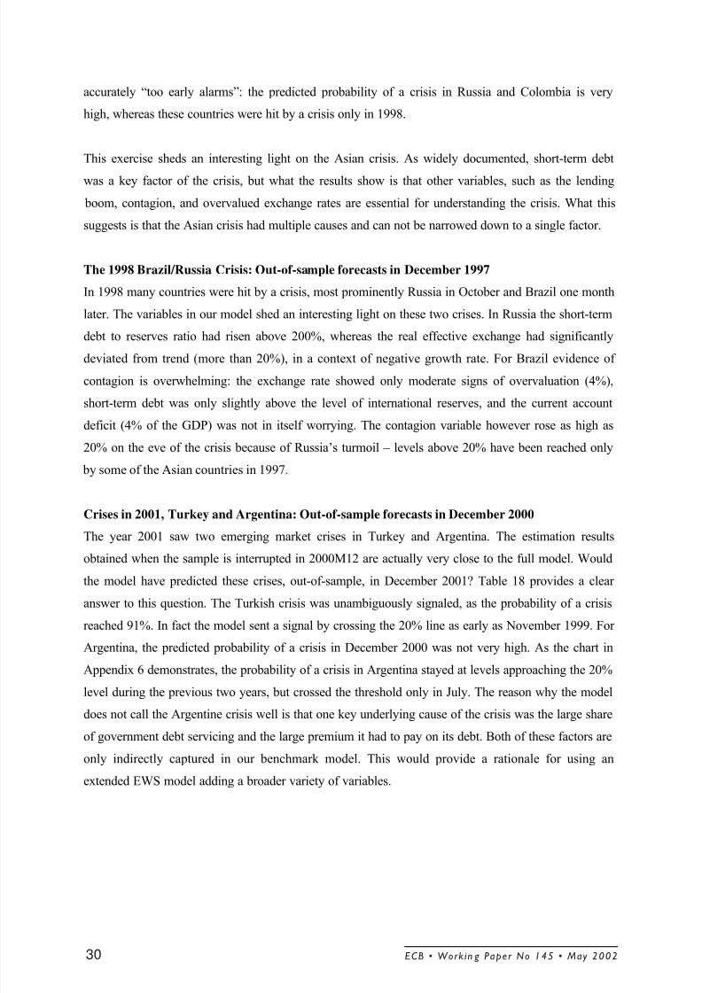
accurately “too early alarms”: the predicted probability of a crisis in Russia and Colombia is very
high, whereas these countries were hit by a crisis only in 1998.
This exercise sheds an interesting light on the Asian crisis. As widely documented, short-term debt
was a key factor of the crisis, but what the results show is that other variables, such as the lending
boom, contagion, and overvalued exchange rates are essential for understanding the crisis. What this
suggests is that the Asian crisis had multiple causes and can not be narrowed down to a single factor.
The 1998 Brazil/Russia Crisis: Out-of-sample forecasts in December 1997
In 1998 many countries were hit by a crisis, most prominently Russia in October and Brazil one month
later. The variables in our model shed an interesting light on these two crises. In Russia the short-term
debt to reserves ratio had risen above 200%, whereas the real effective exchange had significantly
deviated from trend (more than 20%), in a context of negative growth rate. For Brazil evidence of
contagion is overwhelming: the exchange rate showed only moderate signs of overvaluation (4%),
short-term debt was only slightly above the level of international reserves, and the current account
deficit (4% of the GDP) was not in itself worrying. The contagion variable however rose as high as
20% on the eve of the crisis because of Russia’s turmoil – levels above 20% have been reached only
by some of the Asian countries in 1997.
Crises in 2001, Turkey and Argentina: Out-of-sample forecasts in December 2000
The year 2001 saw two emerging market crises in Turkey and Argentina. The estimation results
obtained when the sample is interrupted in 2000M12 are actually very close to the full model. Would
the model have predicted these crises, out-of-sample, in December 2001? Table 18 provides a clear
answer to this question. The Turkish crisis was unambiguously signaled, as the probability of a crisis
reached 91%. In fact the model sent a signal by crossing the 20% line as early as November 1999. For
Argentina, the predicted probability of a crisis in December 2000 was not very high. As the chart in
Appendix 6 demonstrates, the probability of a crisis in Argentina stayed at levels approaching the 20%
level during the previous two years, but crossed the threshold only in July. The reason why the modeldoes not call the Argentine crisis well is that one key underlying cause of the crisis was the large share
of government debt servicing and the large premium it had to pay on its debt. Both of these factors are
only indirectly captured in our benchmark model. This would provide a rationale for using an
extended EWS model adding a broader variety of variables.
ECB • Work in g Paper No 145 • May 200230
8/3/2019 Early Warning System Europe
http://slidepdf.com/reader/full/early-warning-system-europe 32/67
Table 17: Estimation results, out-of-sample forecasts
Model Benchmark End point:1996M12
End point:1997M12
End point:
2000M12Over-valuation
***0.161(0.013)
***0.120(0.021)
***0.135(0.015)
***0.167(0.013)
LendingBoom
***0.013(0.002)
***0.016(0.003)
***0.018(0.003)
***0.013(0.002)
STD/res ***0.004(0.001)
-0.001(0.002)
**0.002(0.001)
***0.004(0.001)
CA/GDP ***-0.055(0.017)
-0.008(0.029)
0.002(0.019)
***-0.055(0.017)
FinancialContagion
***0.039(0.015)
*0.063(0.038)
***0.084(0.031)
***0.044(0.015)
Growth ***-0.060
(0.023)
*-0.067
(0.040)
-0.040
(0.034)
**-0.054
(0.023)Constant ***-2.866
(0.215)
***-2.015
(0.394)
***-2.345
(0.337)
***-2.866
(0.221)# obs 1549 590 818 1501
Pseudo R2 0.333 0.317 0.308 0.344
Table 18: Predicted probabilities, out-of-sample forecasts
Country Out of SampleEnd date:1996M12
CrisisIn 1997
Out of SampleEnd date:1997M12
CrisisIn1998
Out of SampleEnd date:2000M12
CrisisIn2001
Argentina 0.038 No 0.151 No 0.134 2001M3Brazil 0.121 No 0.362 98M10 0.065 NoChile 0.111 No 0.368 98M9 0.011 NoChina 0.088 No 0.191 No 0.053 NoColombia 0.685 No 0.422 98M9 0.002 No
Czech Rep. 0.141 97M5 0.03 No 0.030 NoH.-Kong 0.164 No 0.711 98M8 0.013 NoHungary 0.063 No 0.036 No 0.002 NoIndonesia 0.480 97M8 0.004 No 0.014 NoKorea 0.167 97M11 0.002 No 0.080 No
Malaysia 0.305 97M7 0.031 No 0.028 NoMexico 0.003 No 0.036 No 0.555 No
Philippines 0.680 97M10 0.125 No 0.001 NoPoland 0.114 No 0.120 No 0.090 No
Russia 0.329 No 0.881 98M9 0.026 NoSingapore 0.167 97M10 0.179 No 0.008 NoThailand 0.340 97M7 0.002 No 0.018 NoTurkey 0.010 No 0.166 No 0.914 2000M12Venezuela 0.001 No 0.111 No 0.172 No
Note: For Turkey the predicted probability of a crisis actually passed 20% in 1999M11.
ECB • Work ing Paper No 14 5 • May 2002 31
8/3/2019 Early Warning System Europe
http://slidepdf.com/reader/full/early-warning-system-europe 33/67
6 Policy Relevance of the Multinomial Logit EWS Model
The purpose of this section is to show how changes to the preferences of the policy-maker and the
specification of the loss function and its parameters can fundamentally alter the design of the optimal
type of model a policy-maker may wish to choose.
Tables 12 and 13 above shows the results of the multinomial logit EWS model for a time horizon of
12 months prior to a crisis and at a probability threshold of 20%. However, the time horizon and the
probability threshold are endogenous choices that a policy-maker can decide. These choices depend on
the loss function of the policy-maker, i.e. how she weights the benefit from receiving a correct signal
about a pending crisis relative to the cost of sending a wrong signal and the cost of missing a crisis.
For a decision-maker, taking pre-emptive action in response to a signal about a possible crisis is
costly. But also not receiving a signal when a crisis actually occurs can be costly if early action by the
policy-maker may could have helped prevent or at least lessen the impact of a crisis.
6.1 Loss function for the policy-maker
As discussed briefly in section 2.3, the first difficult choice for a policy-maker is which objective
function to optimize. Clearly, a policy-maker wishes to extract as many correct signals as early in
advance as possible about the occurrence of a crisis. On the contrary, she would like to minimize the
number of false alarms (i.e. when the model issues a signal but no crisis occurs) and the number of
missed crises (when the model yields no signal but a crisis ensues). The difficulty with the latter is that
there is a trade-off between the number of false alarms and the number of missed crises: raising the
probability threshold T and lengthening the time horizon length H reduces the number of false alarms,
but at the cost of raising the number of missed crises months. Lowering the threshold T and shortening
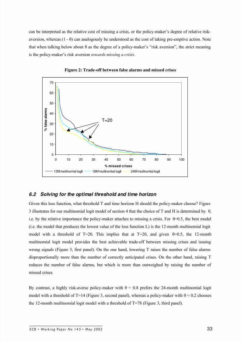
the time horizon length H will accordingly lead to the opposite trade-off. Figure 2 illustrates this trade-
off for all thresholds T and for three time-horizon models (12 months, 18 months and 24 months).
Which of the models and thresholds a policy-makers wishes to choose depends on the form of her
objective function. Assume that missing a crisis as well as issuing a signal that requires taking pre-
emptive action both have a cost for the policy-maker, which she wants to minimize. Therefore the loss
function of the policy-maker is formulated as
( ) )(1)()( / T probT probT L SC NS θ θ −+≡ (13)
with prob NS/C
as the probability of a missed crisis, i.e. the joint probability that the EWS model issuesno signal and a crisis occurs, and probS as the probability of issuing a signal that a crisis will occur. θ
ECB • Work in g Paper No 145 • May 200232
8/3/2019 Early Warning System Europe
http://slidepdf.com/reader/full/early-warning-system-europe 34/67
can be interpreted as the relative cost of missing a crisis, or the policy-maker’s degree of relative risk-
aversion, whereas (1 - θ) can analogously be understood as the cost of taking pre-emptive action. Note
that when talking below about θ as the degree of a policy-maker’s “risk aversion”, the strict meaning
is the policy-maker’s risk aversion towards missing a crisis.
Figure 2: Trade-off between false alarms and missed crises
6.2 Solving for the optimal threshold and time horizon
Given this loss function, what threshold T and time horizon H should the policy-maker choose? Figure
3 illustrates for our multinomial logit model of section 4 that the choice of T and H is determined by θ,
i.e. by the relative importance the policy-maker attaches to missing a crisis. For θ=0.5, the best model
(i.e. the model that produces the lowest value of the loss function L) is the 12-month multinomial logit
model with a threshold of T=20. This implies that at T=20, and given θ=0.5, the 12-month
multinomial logit model provides the best achievable trade-off between missing crises and issuing
wrong signals (Figure 3, first panel). On the one hand, lowering T raises the number of false alarms
disproportionally more than the number of correctly anticipated crises. On the other hand, raising T
reduces the number of false alarms, but which is more than outweighed by raising the number of
missed crises.
By contrast, a highly risk-averse policy-maker with θ = 0.8 prefers the 24-month multinomial logit
model with a threshold of T=14 (Figure 3, second panel), whereas a policy-maker with θ = 0.2 chooses
the 12-month multinomial logit model with a threshold of T=78 (Figure 3, third panel).
0
10
20
30
40
50
60
70
0 10 20 30 40 50 60 70 80 90 100
% missed crises
% f a
l s e
a l a r m s
12M multinomial logit 18M multinomial logit 24M multinomial logit
T=20
ECB • Work ing Paper No 14 5 • May 2002 33
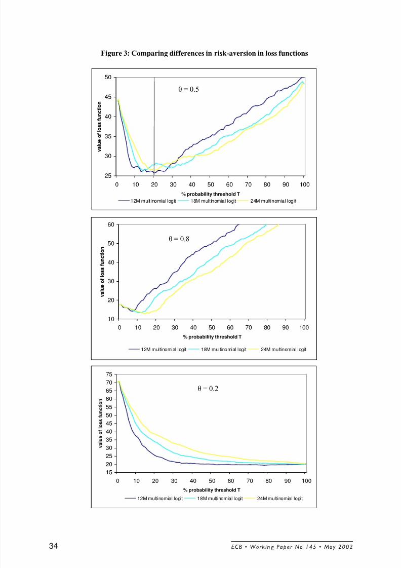
8/3/2019 Early Warning System Europe
http://slidepdf.com/reader/full/early-warning-system-europe 35/67
Figure 3: Comparing differences in risk-aversion in loss functions
25
30
35
40
45
50
0 10 20 30 40 50 60 70 80 90 100
% probability threshold T
v a l u e o f l o s s f u n c t i o n
12M multinomial logit 18M multinomial logit 24M multinomial logit
15
20
25
30
35
40
45
50
5560
65
70
75
0 10 20 30 40 50 60 70 80 90 100
% probability threshold T
v a l u e o f l o s s f u n c t i o n
12M multinomial logit 18M multinomial logit 24M multinomial logit
10
20
30
40
50
60
0 10 20 30 40 50 60 70 80 90 100
% probability threshold T
v a l u e o f l o s s f u n c t i o n
12M multinomial logit 18M multinomial logit 24M multinomial logit
θ = 0.5
θ = 0.8
θ = 0.2
ECB • Work in g Paper No 145 • May 200234
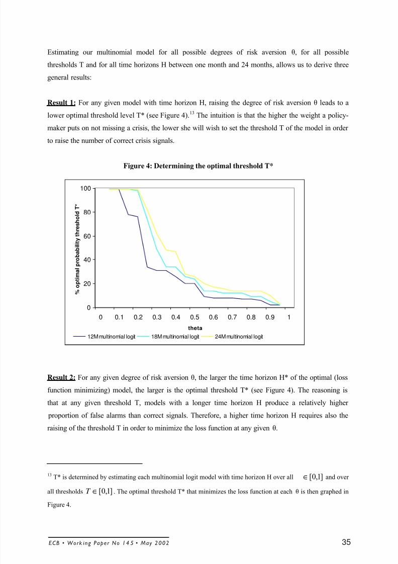
8/3/2019 Early Warning System Europe
http://slidepdf.com/reader/full/early-warning-system-europe 36/67
Estimating our multinomial model for all possible degrees of risk aversion θ, for all possible
thresholds T and for all time horizons H between one month and 24 months, allows us to derive three
general results:
Result 1: For any given model with time horizon H, raising the degree of risk aversion θ leads to a
lower optimal threshold level T* (see Figure 4).13
The intuition is that the higher the weight a policy-
maker puts on not missing a crisis, the lower she will wish to set the threshold T of the model in order
to raise the number of correct crisis signals.
Figure 4: Determining the optimal threshold T*
Result 2: For any given degree of risk aversion θ, the larger the time horizon H* of the optimal (loss
function minimizing) model, the larger is the optimal threshold T* (see Figure 4). The reasoning is
that at any given threshold T, models with a longer time horizon H produce a relatively higher
proportion of false alarms than correct signals. Therefore, a higher time horizon H requires also the
raising of the threshold T in order to minimize the loss function at any given θ.
13T* is determined by estimating each multinomial logit model with time horizon H over all ]1,0[∈ and over
all thresholds ]1,0[∈T . The optimal threshold T* that minimizes the loss function at each θ is then graphed in
Figure 4.
0
20
40
60
80
100
0 0.1 0.2 0.3 0.4 0.5 0.6 0.7 0.8 0.9 1
theta
% o
p t i m a l p r o b a b i l i t y t h r e s h o l d T *
12M multinomial logit 18M multinomial logit 24M multinomial logit
ECB • Work ing Paper No 14 5 • May 2002 35
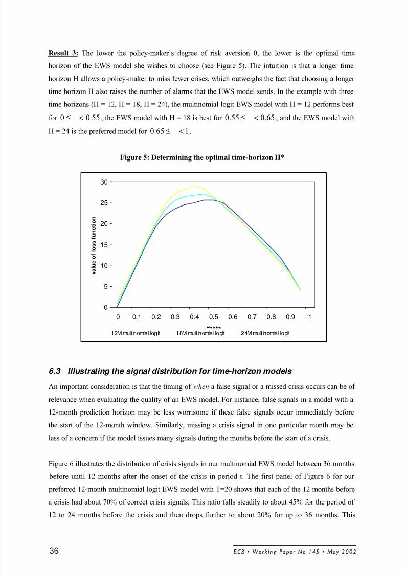
8/3/2019 Early Warning System Europe
http://slidepdf.com/reader/full/early-warning-system-europe 37/67
Result 3: The lower the policy-maker’s degree of risk aversion θ, the lower is the optimal time
horizon of the EWS model she wishes to choose (see Figure 5). The intuition is that a longer time
horizon H allows a policy-maker to miss fewer crises, which outweighs the fact that choosing a longer
time horizon H also raises the number of alarms that the EWS model sends. In the example with three
time horizons (H = 12, H = 18, H = 24), the multinomial logit EWS model with H = 12 performs best
for 55.00 <≤ , the EWS model with H = 18 is best for 65.055.0 <≤ , and the EWS model with
H = 24 is the preferred model for 165.0 <≤ .
Figure 5: Determining the optimal time-horizon H*
6.3 Illustrating the signal distribution for time-horizon models
An important consideration is that the timing of when a false signal or a missed crisis occurs can be of
relevance when evaluating the quality of an EWS model. For instance, false signals in a model with a12-month prediction horizon may be less worrisome if these false signals occur immediately before
the start of the 12-month window. Similarly, missing a crisis signal in one particular month may be
less of a concern if the model issues many signals during the months before the start of a crisis.
Figure 6 illustrates the distribution of crisis signals in our multinomial EWS model between 36 months
before until 12 months after the onset of the crisis in period t. The first panel of Figure 6 for our
preferred 12-month multinomial logit EWS model with T=20 shows that each of the 12 months before
a crisis had about 70% of correct crisis signals. This ratio falls steadily to about 45% for the period of
12 to 24 months before the crisis and then drops further to about 20% for up to 36 months. This
0
5
10
15
20
25
30
0 0.1 0.2 0.3 0.4 0.5 0.6 0.7 0.8 0.9 1
theta
v a l u e o f l o s s f u n c t i o n
12M multinomial logit 18M multinomial logit 24M multinomial logit
ECB • Work in g Paper No 145 • May 200236
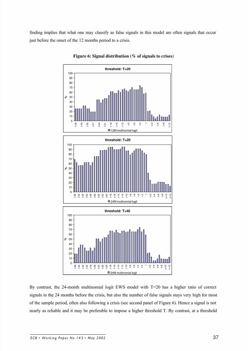
8/3/2019 Early Warning System Europe
http://slidepdf.com/reader/full/early-warning-system-europe 38/67
finding implies that what one may classify as false signals in this model are often signals that occur
just before the onset of the 12 months period to a crisis.
Figure 6: Signal distribution (% of signals to crises)
By contrast, the 24-month multinomial logit EWS model with T=20 has a higher ratio of correct
signals in the 24 months before the crisis, but also the number of false signals stays very high for most
of the sample period, often also following a crisis (see second panel of Figure 6). Hence a signal is not
nearly as reliable and it may be preferable to impose a higher threshold T. By contrast, at a threshold
threshold: T=20
0
10
20
30
40
50
60
70
80
90
100
t - 3 6
t - 3 3
t - 3 0
t - 2 7
t - 2 4
t - 2 1
t - 1 8
t - 1 5
t - 1 2
t - 9
t - 6
t - 3 t
t + 3
t + 6
t + 9
t + 1 2
%
12M multinomial logit
threshold: T=20
0
10
20
30
40
50
60
70
80
90
100
t - 3 6
t - 3 4
t - 3 2
t - 3 0
t - 2 8
t - 2 6
t - 2 4
t - 2 2
t - 2 0
t - 1 8
t - 1 6
t - 1 4
t - 1 2
t - 1 0
t - 8
t - 6
t - 4
t - 2 t
t + 2
t + 4
t + 6
t + 8
t + 1 0
t + 1 2
%
24M multinomial logit
threshold: T=40
0
10
20
30
40
50
60
70
80
90
100
t - 3 6
t - 3 4
t - 3 2
t - 3 0
t - 2 8
t - 2 6
t - 2 4
t - 2 2
t - 2 0
t - 1 8
t - 1 6
t - 1 4
t - 1 2
t - 1 0
t - 8
t - 6
t - 4
t - 2
t
t + 2
t + 4
t + 6
t + 8
t + 1 0
t + 1 2
%
24M multinomial logit
ECB • Work ing Paper No 14 5 • May 2002 37
8/3/2019 Early Warning System Europe
http://slidepdf.com/reader/full/early-warning-system-europe 39/67
of T=40, the 24-month model performs similarly to the 12-month EWS model with T=20 (see third
panel of Figure 6).
7 Conclusions
This paper developed a new Early Warning System (EWS) model for predicting financial crises, based
on a multinomial logit model approach. Its main difference to existing EWS models and its intended
contribution to the literature focused on three areas. First, it discussed what we call the “post-crisis”
bias in the existing binomial discrete-dependent-variable EWS models and showed that failing to
distinguish between pre-crisis and post-crisis periods may introduce a bias in the estimation results. By
contrast, the use of a multinomial logit allows the distinction between more than two regimes and
allows solving for this type of bias.
The second area is that our EWS model employs a number of relevant economic variables that have
not been used before for the purpose of EWS models. In particular, we find that the use of contagion
variables, which takes into account that crises are often not isolated events but interconnected across
economies, helps improve the predictive power of EWS models. And third, the paper developed a
framework that allows policy-makers to design the features of their EWS model according to their
preferences and degree of risk-aversion.
The paper showed that taking into account these methodological issues can indeed help improve the
performance of EWS models substantially. In particular, moving from a binomial logit model to a
multinomial logit model with three regimes improves the predictive power of the EWS. Overall, the
EWS based on the multinomial logit model predicts well most currency crises in emerging markets
during the 1990s, both in-sample as well as out-of-sample. For the in-sample estimation, the model
fails to anticipate only two of the emerging market crises in our sample. For the out-of-sample
estimation, the model for instance would have anticipated correctly most of the countries that
succumbed to the Asian crisis.
It should be emphasized that the EWS model developed in this paper does certainly not constitute the
final step towards a comprehensive EWS model of financial crises. However, we believe that by
outlining existing methodological difficulties and by suggesting a new method to solve some of these
problems, the paper constitutes a further step towards developing an EWS model that could become an
even more powerful tool for policy-makers in the future. Future research on EWS models may focus
on adding dynamic components to EWS models, and in particular by addressing the current
endogeneity of the choice of the timing and the length of different regimes. This may be
ECB • Work in g Paper No 145 • May 200238
8/3/2019 Early Warning System Europe
http://slidepdf.com/reader/full/early-warning-system-europe 40/67
accomplished, for instance, by utilizing regime-switching models that have already been employed
successfully in other areas of economic forecasting.
From a policy perspective, developing Early Warning System (EWS) models that help to reliably
anticipate financial crises could become an even more important tool for policy-makers in the future.
Many financial crises over the past few decades had devastating social, economic and political
consequences. Developing reliable EWS models therefore can be of substantial value by allowing
policy-makers to obtain clear signals when and how to take pre-emptive measures in order to mitigate
or even prevent financial turmoil. It should be stressed that EWS models can not replace the sound
judgment of the policy-maker to guide policy, but it can play an important complementary role as a
neutral and objective measure of vulnerability.
ECB • Work ing Paper No 14 5 • May 2002 39
8/3/2019 Early Warning System Europe
http://slidepdf.com/reader/full/early-warning-system-europe 41/67
ECB • Work in g Paper No 145 • May 200240
References
Berg, Andrew, Eduardo Borensztein, and Catherine Pattillo, 2001, “Assessing Early WarningSystems: How Have They Worked in Practice?”, IMF mimeo, October 2001.
Berg, Andrew and Catherine Pattillo, 1999a, “Are Currency Crises Predictable? A Test”, IMF Staff Papers; 46(2), June 1999, pp. 107-38.
Berg, Andrew and Catherine Pattillo, 1999b, “Predicting Currency Crises: The Indicators Approachand an Alternative”, Journal of International Money and Finance; 18(4), August 1999, pp. 561-86.
Bussiere, Matthieu, Book Review, “Assessing Financial Vulnerability: An Early Warning System for Emerging Markets”, by M. Goldstein, G. Kaminsky, C. Reinhart; International Journal of Financeand Economics, April 2001, Volume 6, Issue 2, pp. 185.
Bussiere, Matthieu and Christian Mulder, 1999, “External Vulnerability in Emerging MarketEconomies: How High Liquidity Can Offset Weak Fundamentals and the Effects of Contagion”, IMFWorking Paper, WP/99/88.
Bussiere, Matthieu and Christian Mulder, 2001, "Which short-term debt over reserve ratio works best?", Chapter 6 in Capital Flows Without Crisis? Reconciling Capital Mobility and EconomicStability, Dipak Dasgupta , Marc Uzan, Dominic Wilson eds., Routlege, July 2001, 206 pages.
Calvo, Guillermo A., and Enrique Mendoza. (2000). Rational Contagion and the Globalization of
Securities Markets. Journal of International Economics. (51), pp. 79-113.
Credit Suisse First Boston (CSFB), 2001, Emerging Market Risk Indicator (EMRI): Re-estimated
Version September 2000, by Amlan Roy and Maria M. Tudela, February 2001.
Demirguc-Kunt, Asli, and Enrica Detragiache, 1999, “Monitoring Banking Sector Fragility: AMultivariate Logit Approach”, World Bank Economic Review, 14 (2), May 2000, pp. 287-307.
Demirguc-Kunt, Asli, and Enrica Detragiache, 1998, “The Determinants of Banking Crises inDeveloping and Developed Countries”, IMF Staff Papers, Volume 45, Number 1, March 1998.
Deutsche Bank, 2000, Deutsche Bank Alarm Clock (DBAC): Forecasting Exchange Rate and Interest
Rate Events in Emerging Markets, by Peter Garber, Robin L. Lumsdaine, and Marco van der Leij,October 2000.
Edison, Hali J., 2000, “Do Indicators of Financial Crisis Work? An Evaluation of an Early WarningSystem,” International Finance Working Paper No. 675, Board of Governors of the Federal Reserve
System.
Eichengreen, Barry, Andrew Rose and Charles Wyplosz, 1995, “Exchange Market Mayhem: TheAntecedents and Aftermaths of Speculative Attacks”, Economic Policy, 21, pp. 249-312.
Feldstein, Martin, 1999, “Self-Protection for Emerging Market Economies”, NBER Working Paper ,WP 6907, January 1999.
Flood, Robert P., Nancy P. Marion. (1998). “Perspectives on the Recent Currency Crises Literature”. NBER Working Paper No. 6380.
8/3/2019 Early Warning System Europe
http://slidepdf.com/reader/full/early-warning-system-europe 42/67
ECB • Work ing Paper No 14 5 • May 2002 41
Forbes, Kristin and Roberto Rigobon, 1999, “No Contagion, only Interdependence”, NBER WorkingPaper No. 7267.
Frankel, Jeffrey and Andrew Rose, 1996, “Currency Crashes in emerging Markets: an EmpiricalTreatment”, Journal of International Economics, 41, pp. 351-66.
Fratzscher, Marcel, 1998, “Why Are Currency Crises Contagious? A Comparison of the Latin
American Crisis of 1994-1995 and the Asian Crisis of 1997-1998”, Weltwirtschaftliches Archiv/Review of World Economics; 134(4), 1998, pp. 664-91.
Fratzscher, Marcel, 1999, “What Causes Currency Crises: Sunspots, Contagion or Fundamentals?”, European University Institute Working Paper 99/39.
Fratzscher, Marcel, 2002, “On Currency Crises and Contagion”, European Central Bank Working
Paper No. 139, April 2002.
Glick, Reuven, and Andrew Rose, 1999, “Contagion and Trade: Why are Currency Crises Regional?”, Journal of International Money and Finance. No. 18 (4), pp. 603-18.
Goldman Sachs, 1998, GS-Watch: A New Framework for Predicting Financial Crises in Emerging Markets, by Alberto Ades, Rumi Masih, and Daniel Tenengauzer, December 1998.
Goldstein, Morris, Graziela L. Kaminsky and Carmen M. Reinhart, Assessing Financial Vulnerability, An Early Warning System for Emerging Markets, June 2000, Institute for International Economics.
J.P. Morgan, 1998, Event Risk Indicator Handbook , by Avinash D. Persaud, May 1998.
Kamin, Steven, 1999, “The Current International Financial Crisis: How Much Is New ?”, Journal of
International Money and Finance; 18(4), August 1999, pp. 501-514.
Kamin, Steven, John Schindler, and Shawna Samuel, 2001, “The Contribution of Domestic and
External Factors to Emerging Market Devaluation Crises: An Early Warning Systems Approach”,International Finance Working Paper No. 711, Board of Governors of the Federal Reserve System.
Kamin, Steven and Sergio Schmukler, 1999, “What Triggers Market Jitters: A Chronicle of the AsianCrisis”, Board of Governors of the Federal Reserve System, International Finance Discussion Papers Number 634, April 1999.
Kamin, Steven and Oliver Babson, 1999, “The Contribution of Domestic and External Factors to Latin
American Devaluation Crises: An Early Warning Systems Approach”, Board of Governors of the
Federal Reserve System, International Finance Discussion Papers Number 645, September 1999.
Kaminsky, Graciela L. and Carmen M. Reinhart, 1998, “Financial Crises in Asia and Latin America:Then and Now”, American Economic Review, Papers and Proceedings; 88(2), May 1998, pp. 444-48.
Kaminsky, Graciela L. and Carmen M. Reinhart, “The Twin Crises: The Causes of Banking and
Balance-of-Payments Problems”, American Economic Review; 89(3), June 1999, pp. 473-500.
Kaminsky, Graciela L. and Carmen M. Reinhart, 2000, “On Crises, Contagion, and Confusion”; Journal of International Economics; 51(1), June 2000, pp. 145-68.
Kaminsky Graciela L., Saul Lizondo and Carmen M. Reinhart, 1998, “Leading Indicators of CurrencyCrises,” IMF Staff Papers, 45, No. 1, pp. 1-48.
8/3/2019 Early Warning System Europe
http://slidepdf.com/reader/full/early-warning-system-europe 43/67
ECB • Work in g Paper No 145 • May 200242
Krugman, Paul, 1979, “A Model of Balance-of-Payments crises”, Journal of Money, Credit and Banking , Vol. 11 (August), pp. 311-25.
Maddala, G.S., Limited-dependent and Qualitative Variables in Econometrics, Econometric SocietyMonographs, Cambridge University Press, 1989.
Milesi-Ferretti, Gian-Maria and Assaf Razin, 1996, “Persistent Current Account Deficits: A Warning
Signal ?”, International Journal of Finance and Economics, 1, pp. 161-181 (1996).
Morgan Stanley Dean Witter, 2001, An Early Warning System for Currency Crises, by KarinKimbrough and Stephen Li Jen, July 2001.
Sachs, Jeffrey, Aaron Tornell and Andres Velasco, 1996, “The Mexican Peso Crisis: Sudden Death Or Death Foretold ?”, Journal of International Economics 41 (1996), pp. 265-283.
Sachs, Jeffrey, Aaron Tornell and Andres Velasco, 1996, “Financial Crises in Emerging Markets: The
Lessons from 1995”, Brookings Papers on Economic Activity; 10(1), 1996: 147-98.
Schnatz, Bernd, 1999, "The Sudden Freeze of the Asian Miracle: The Role of MacroeconomicFundamentals", Asia Pacific Journal of Finance, Volume 2, Issue 1, May 1999.
Schnatz, Bernd, 1998, “Macroeconomic Determinants of currency turbulences in emerging markets”,Discussion paper 3/98, Economic Research Group of the Deutsche Bundesbank, September 1998.
Tornell, Aaron, 1999, “Common Fundamentals in the Tequila and Asian Crises”, National Bureau of Economic Research Working Paper, 7139, May 1999.
Van Rijckeghem, Caroline, and Beatrice Weder. (1999). Sources of Contagion: Finance or Trade?
International Monetary Fund Working Paper No. 146.
Weber, Axel A., 1997, “Sources of Currency Crises: An Empirical Analysis”, Universitaet Bonn
Discussion Paper No. B-418.
Zanello, Alessandro and Dominique Desruelle, 1997, “A Primer on the IMF's Information NoticeSystem”, IMF Working Paper , WP 97/71.
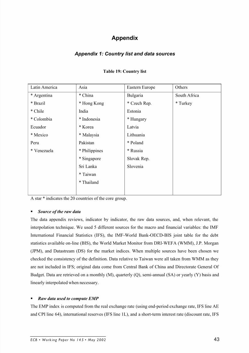
8/3/2019 Early Warning System Europe
http://slidepdf.com/reader/full/early-warning-system-europe 44/67
ECB • Work ing Paper No 14 5 • May 2002 43
Appendix
Appendix 1: Country list and data sources
Table 19: Country list
Latin America Asia Eastern Europe Others
* Argentina
* Brazil
* Chile
* Colombia
Ecuador
* Mexico
Peru
* Venezuela
* China
* Hong Kong
India
* Indonesia
* Korea
* Malaysia
Pakistan
* Philippines
* Singapore
Sri Lanka
* Taiwan
* Thailand
Bulgaria
* Czech Rep.
Estonia
* Hungary
Latvia
Lithuania
* Poland
* Russia
Slovak Rep.
Slovenia
South Africa
* Turkey
A star * indicates the 20 countries of the core group.
§ Source of the raw data
The data appendix reviews, indicator by indicator, the raw data sources, and, when relevant, the
interpolation technique. We used 5 different sources for the macro and financial variables: the IMF
International Financial Statistics (IFS), the IMF-World Bank-OECD-BIS joint table for the debt
statistics available on-line (BIS), the World Market Monitor from DRI-WEFA (WMM), J.P. Morgan
(JPM), and Datastream (DS) for the market indices. When multiple sources have been chosen we
checked the consistency of the definition. Data relative to Taiwan were all taken from WMM as they
are not included in IFS; original data come from Central Bank of China and Directorate General Of
Budget. Data are retrieved on a monthly (M), quarterly (Q), semi-annual (SA) or yearly (Y) basis and
linearly interpolated when necessary.
§ Raw data used to compute EMP
The EMP index is computed from the real exchange rate (using end-period exchange rate, IFS line AE
and CPI line 64), international reserves (IFS line 1L), and a short-term interest rate (discount rate, IFS
8/3/2019 Early Warning System Europe
http://slidepdf.com/reader/full/early-warning-system-europe 45/67
ECB • Work in g Paper No 145 • May 200244
line 60, money market rate, IFS line 60B, deposit interest rate IFS line 60L, lending interest rate IFS
line 60P).
The default is the money market rate (IFS line 60b), we used the lending rate (IFS Line 60P) for Chile,China, the deposit rate (IFS line 60L) for Colombia, the Czech Rep., Ecuador, Hungary, Peru,
Philippines, Slovakia, and Venezuela.
We transformed the raw EMP using a three-month moving average with weights 3/6, 2/6 and 1/6 for
time t, t-1 and t-2 respectively. This transformation is similar to Schnatz (1998, 1999) who used
geometric weights, to which we refer for a detailed discussion of methodological issues in the design
of the crisis index.
§ Real effective exchange rate
For Chile, China, Col., Czech Rep., Ecuador, Estonia, Hungary, Korea, Malaysia, Mexico, Pakistan,
Philippines, Poland, Russia, Slovak Republic, South Africa, Turkey, data were taken from WMM and
for Argentina, Brazil, Bulgaria, Hong Kong, India, Indonesia, Peru, Singapore, Slovenia, Taiwan,
Thailand, from JPM. The data from WMM come from IMF (see Desruelles and Zanello, 1997 for a
presentation of the IMF definition of the REER) or closely follow this methodology.
§ GDP
Nominal and real GDP were taken from WMM and interpolated from Q data. For Pakistan and Sri
Lanka data are from IFS line 99b (A frequency).
§ Current account items
Exports are taken from IFS line 70 and imports from IFS line 71. Current account was taken from
WMM and linearly interpolated from Q to M frequency , except for China (IFS, A frequency). Ratio’s
are expressed in percentage of the GDP using the nominal monthly exchange rate. The series were
transformed using a 12 month moving average with equal weights: this allowed to remove seasonality
and sometimes strong volatility, and in addition it allows a more reliable assessment of the situation by
looking at flows on the past year instead of the last month.
§ Government deficit
The government deficit is available at a monthly frequency from IFS line 80. Exception were Chile,
China, Estonia, India, Indonesia, Pakistan, Slovak Republic, Sri Lanka, Turkey (A), for Hong Kong,
Malaysia, Poland data were taken from WMM (Q). The same transformation as for the current account
was undertaken.
8/3/2019 Early Warning System Europe
http://slidepdf.com/reader/full/early-warning-system-europe 46/67
ECB • Work ing Paper No 14 5 • May 2002 45
§ Monetary variables
Source is IFS line 34 for M1 and line 35 for quasi-money (M2 is obtained adding line 34 and line 35).
Domestic credit is taken from IFS line 32, credit to the government sector (central government) from
line 32an, credit to the private sector from line 32b.
§ Financial account capital flows
WMM was the source for foreign direct investment, exports, imports, and net flows, for portfolio
investment, assets, liabilities, and net flows.
§ Debt statistics
The BIS database on debt statistics includes the following series that we downloaded: bank loans (BIS
Line A), Brady Bonds (Line C), liabilities within one year (Line G), total liabilities, locational concept
(Line J), total liabilities, consolidated concept (Line K).
§ Trade data
Bilateral trade data come from the World Trade Analyzer.
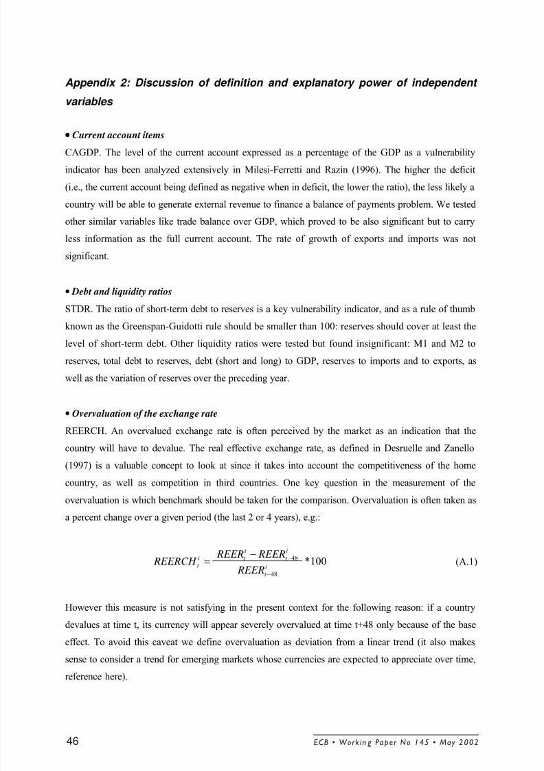
8/3/2019 Early Warning System Europe
http://slidepdf.com/reader/full/early-warning-system-europe 47/67
Appendix 2: Discussion of definition and explanatory power of independent
variables
•••• Current account items
CAGDP. The level of the current account expressed as a percentage of the GDP as a vulnerability
indicator has been analyzed extensively in Milesi-Ferretti and Razin (1996). The higher the deficit
(i.e., the current account being defined as negative when in deficit, the lower the ratio), the less likely a
country will be able to generate external revenue to finance a balance of payments problem. We tested
other similar variables like trade balance over GDP, which proved to be also significant but to carry
less information as the full current account. The rate of growth of exports and imports was not
significant.
• Debt and liquidity ratios
STDR. The ratio of short-term debt to reserves is a key vulnerability indicator, and as a rule of thumb
known as the Greenspan-Guidotti rule should be smaller than 100: reserves should cover at least the
level of short-term debt. Other liquidity ratios were tested but found insignificant: M1 and M2 to
reserves, total debt to reserves, debt (short and long) to GDP, reserves to imports and to exports, as
well as the variation of reserves over the preceding year.
• Overvaluation of the exchange rate
REERCH. An overvalued exchange rate is often perceived by the market as an indication that the
country will have to devalue. The real effective exchange rate, as defined in Desruelle and Zanello
(1997) is a valuable concept to look at since it takes into account the competitiveness of the home
country, as well as competition in third countries. One key question in the measurement of the
overvaluation is which benchmark should be taken for the comparison. Overvaluation is often taken as
a percent change over a given period (the last 2 or 4 years), e.g.:
100*48
48
i
t
i
t
i
t i
t REER
REER REER REERCH
−
−−= (A.1)
However this measure is not satisfying in the present context for the following reason: if a country
devalues at time t, its currency will appear severely overvalued at time t+48 only because of the base
effect. To avoid this caveat we define overvaluation as deviation from a linear trend (it also makes
sense to consider a trend for emerging markets whose currencies are expected to appreciate over time,
reference here).
ECB • Work in g Paper No 145 • May 200246

8/3/2019 Early Warning System Europe
http://slidepdf.com/reader/full/early-warning-system-europe 48/67
( )100*
i
t
i
t
i
t i
t TREND
TREND REER REERDEV
−= (A.2)
• Real variables
GROWTH. The rate of growth of real output can play an important role is avoiding crises for two
reasons: first it will generate with more difficulty the revenues necessary to pay back the debt burden
and second a government may be more reluctant to implement stabilization programs if output is
already slowing down.
• Financial sector fragilities
As the Twin crises argument has met a lot of empirical support since it was started by Kaminsky and
Reinhart (1996), EWS models have given an increasing importance to financial sector fragility. The presence of bad loans in the banking sector has often been put forward as a key determinant of the
Asian crisis (references). Such variables are however more difficult to collect than the other variables
listed above because they are not directly observable. Bad loans for instance are subject to notorious
under-reporting. Four types of variables have been considered as proxies:
a) Lending boom index
The increase of the credit to the private sector can give an indication that a country is over-heating. If
the progression of these credits is too rapid, one can suspect that a lot is going to dubious projects.
Empirical evidence so far was not conclusive: earlier contributions (Sachs, Tornell, and Velasco,
1995) were later contradicted by studies pointing out that lending booms can also act as contra-
indicators, noticeably in the case of Russia (Bussiere and Mulder, 1999). The present results should
then be qualified: in many cases a lending boom led to a crisis, but a sharp decrease can also be a sign
of weakness (as exemplified recently in Argentina). This issue deserves further investigation to fix the
debate.
b) Banking sector stock index
The banking sector stock index could proxy banking sector imbalances, assuming that these
imbalances are perfectly evaluated by the markets – an admittedly bold assumption. In fact the
coefficient on this variable turned up to be significant at the 5% level, with the correct sign. However,
we decided not to keep this variable in the model for two reasons: first its contribution to the
predictive power of the model was not conclusive and second problems of comparability across
countries can be more important for this variable as for the others as not all countries have a fully
developed and transparent market where bank indices are freely quoted.
ECB • Work ing Paper No 14 5 • May 2002 47
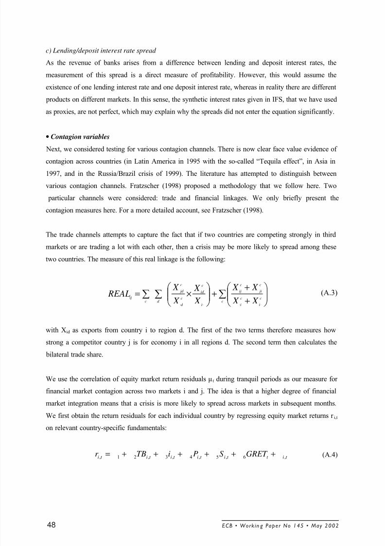
8/3/2019 Early Warning System Europe
http://slidepdf.com/reader/full/early-warning-system-europe 49/67
c) Lending/deposit interest rate spread
As the revenue of banks arises from a difference between lending and deposit interest rates, the
measurement of this spread is a direct measure of profitability. However, this would assume the
existence of one lending interest rate and one deposit interest rate, whereas in reality there are different
products on different markets. In this sense, the synthetic interest rates given in IFS, that we have used
as proxies, are not perfect, which may explain why the spreads did not enter the equation significantly.
• Contagion variables
Next, we considered testing for various contagion channels. There is now clear face value evidence of
contagion across countries (in Latin America in 1995 with the so-called “Tequila effect”, in Asia in
1997, and in the Russia/Brazil crisis of 1999). The literature has attempted to distinguish between
various contagion channels. Fratzscher (1998) proposed a methodology that we follow here. Two
particular channels were considered: trade and financial linkages. We only briefly present the
contagion measures here. For a more detailed account, see Fratzscher (1998).
The trade channels attempts to capture the fact that if two countries are competing strongly in third
markets or are trading a lot with each other, then a crisis may be more likely to spread among these
two countries. The measure of this real linkage is the following:
ååå ÷÷ ø öçç
è æ
+++÷÷
ø öçç
è æ ×=
⋅⋅⋅⋅c
c
i
c
i
c
ji
c
ij
i
cid
c
d
c
jd
d cij
X X X X
X X
X X REAL (A.3)
with Xid as exports from country i to region d. The first of the two terms therefore measures how
strong a competitor country j is for economy i in all regions d. The second term then calculates the
bilateral trade share.
We use the correlation of equity market return residuals µtduring tranquil periods as our measure for
financial market contagion across two markets i and j. The idea is that a higher degree of financial
market integration means that a crisis is more likely to spread across markets in subsequent months.
We first obtain the return residuals for each individual country by regressing equity market returns r i,t
on relevant country-specific fundamentals:
t it t it it it it i GRET SPiTBr ,6,5,4,3,21, ++++++= (A.4)
ECB • Work in g Paper No 145 • May 200248
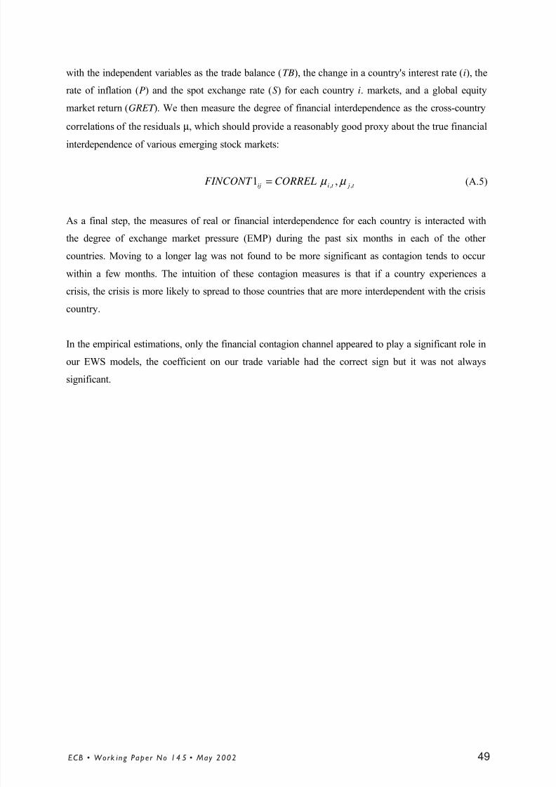
8/3/2019 Early Warning System Europe
http://slidepdf.com/reader/full/early-warning-system-europe 50/67
with the independent variables as the trade balance (TB), the change in a country's interest rate (i), the
rate of inflation (P) and the spot exchange rate (S) for each country i. markets, and a global equity
market return (GRET ). We then measure the degree of financial interdependence as the cross-country
correlations of the residuals µ, which should provide a reasonably good proxy about the true financial
interdependence of various emerging stock markets:
t jt iijCORRELFINCONT ,, ,1 µ µ = (A.5)
As a final step, the measures of real or financial interdependence for each country is interacted with
the degree of exchange market pressure (EMP) during the past six months in each of the other
countries. Moving to a longer lag was not found to be more significant as contagion tends to occur
within a few months. The intuition of these contagion measures is that if a country experiences acrisis, the crisis is more likely to spread to those countries that are more interdependent with the crisis
country.
In the empirical estimations, only the financial contagion channel appeared to play a significant role in
our EWS models, the coefficient on our trade variable had the correct sign but it was not always
significant.
ECB • Work ing Paper No 14 5 • May 2002 49
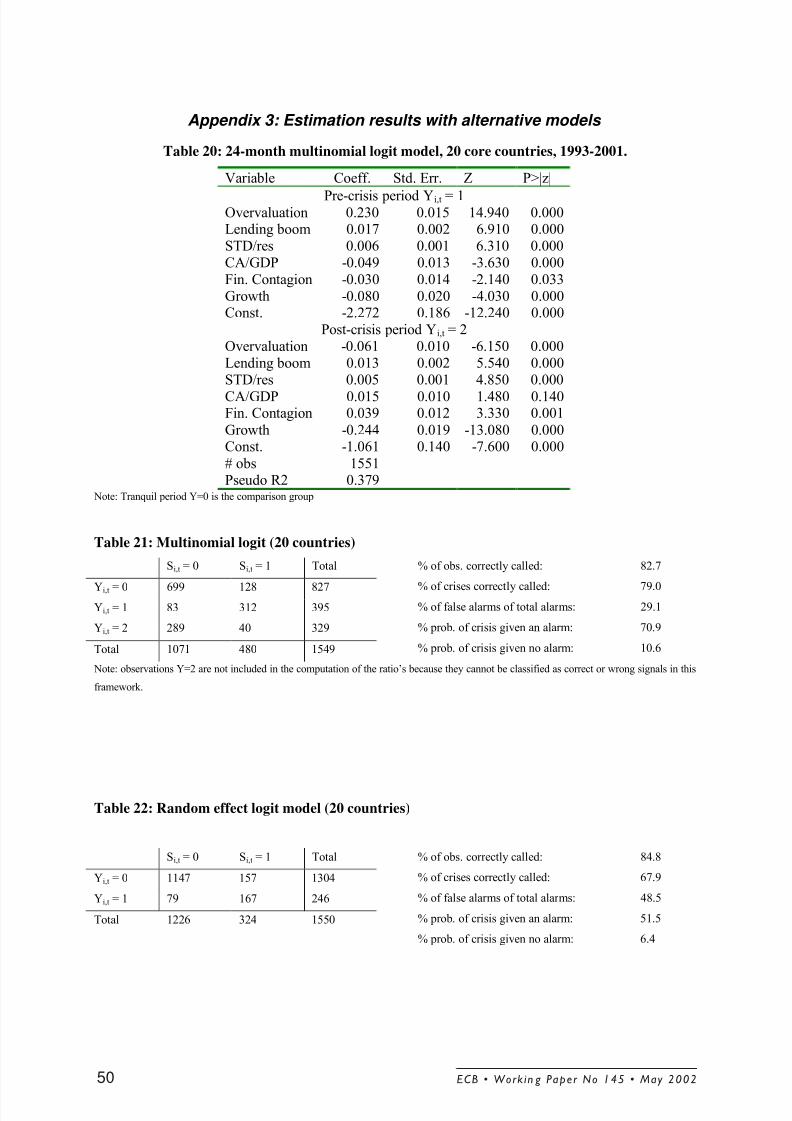
8/3/2019 Early Warning System Europe
http://slidepdf.com/reader/full/early-warning-system-europe 51/67
Appendix 3: Estimation results with alternative models
Table 20: 24-month multinomial logit model, 20 core countries, 1993-2001.
Variable Coeff. Std. Err. Z P>|z|
Pre-crisis period Yi,t = 1Overvaluation 0.230 0.015 14.940 0.000Lending boom 0.017 0.002 6.910 0.000STD/res 0.006 0.001 6.310 0.000CA/GDP -0.049 0.013 -3.630 0.000Fin. Contagion -0.030 0.014 -2.140 0.033Growth -0.080 0.020 -4.030 0.000Const. -2.272 0.186 -12.240 0.000
Post-crisis period Yi,t = 2Overvaluation -0.061 0.010 -6.150 0.000Lending boom 0.013 0.002 5.540 0.000STD/res 0.005 0.001 4.850 0.000
CA/GDP 0.015 0.010 1.480 0.140Fin. Contagion 0.039 0.012 3.330 0.001
Growth -0.244 0.019 -13.080 0.000Const. -1.061 0.140 -7.600 0.000
# obs 1551Pseudo R2 0.379
Note: Tranquil period Y=0 is the comparison group
Table 21: Multinomial logit (20 countries)
Si,t = 0 Si,t = 1 Total
Yi,t = 0 699 128 827Yi,t = 1 83 312 395
Yi,t = 2 289 40 329
Total 1071 480 1549
% of obs. correctly called: 82.7
% of crises correctly called: 79.0% of false alarms of total alarms: 29.1
% prob. of crisis given an alarm: 70.9
% prob. of crisis given no alarm: 10.6
Note: observations Y=2 are not included in the computation of the ratio’s because they cannot be classified as correct or wrong signals in this
framework.
Table 22: Random effect logit model (20 countries)
Si,t = 0 Si,t = 1 Total
Yi,t = 0 1147 157 1304
Yi,t = 1 79 167 246
Total 1226 324 1550
% of obs. correctly called: 84.8
% of crises correctly called: 67.9
% of false alarms of total alarms: 48.5
% prob. of crisis given an alarm: 51.5
% prob. of crisis given no alarm: 6.4
ECB • Work in g Paper No 145 • May 200250
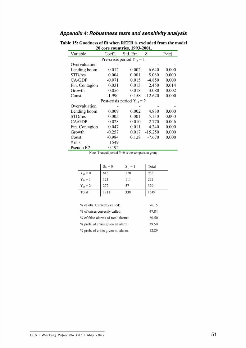
8/3/2019 Early Warning System Europe
http://slidepdf.com/reader/full/early-warning-system-europe 52/67
Appendix 4: Robustness tests and sensitivity analysis
Table 15: Goodness of fit when REER is excluded from the model
20 core countries, 1993-2001.
Variable Coeff. Std. Err. Z P>|z|
Pre-crisis period Yi,t = 1Overvaluation - - - -Lending boom 0.012 0.002 6.640 0.000STD/res 0.004 0.001 5.080 0.000CA/GDP -0.071 0.015 -4.850 0.000Fin. Contagion 0.031 0.013 2.450 0.014Growth -0.056 0.018 -3.080 0.002Const. -1.990 0.158 -12.620 0.000
Post-crisis period Yi,t = 2Overvaluation - - - -Lending boom 0.009 0.002 4.830 0.000STD/res 0.005 0.001 5.130 0.000
CA/GDP 0.028 0.010 2.770 0.006Fin. Contagion 0.047 0.011 4.240 0.000
Growth -0.257 0.017 -15.250 0.000Const. -0.984 0.128 -7.670 0.000# obs 1549Pseudo R2 0.192
Note: Tranquil period Y=0 is the comparison group
Si,t = 0 Si,t = 1 Total
Yi,t = 0 818 170 988
Yi,t = 1 121 111 232
Yi,t = 2 272 57 329
Total 1211 338 1549
% of obs. Correctly called: 76.15
% of crises correctly called: 47.84
% of false alarms of total alarms: 60.50
% prob. of crisis given an alarm: 39.50
% prob. of crisis given no alarm: 12.89
ECB • Work ing Paper No 14 5 • May 2002 51
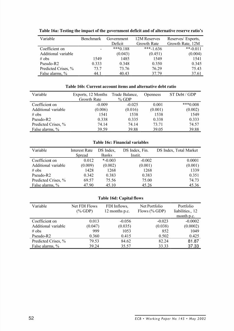
8/3/2019 Early Warning System Europe
http://slidepdf.com/reader/full/early-warning-system-europe 53/67
Table 16a: Testing the impact of the government deficit and of alternative reserve ratio’s
Variable Benchmark GovernmentDeficit
12M ReservesGrowth Rate
Reserves/ Exports,Growth Rate, 12M
Coefficient onAdditional variable
- ***0.188(0.043)
***-1.636(0.451)
**-0.011(0.004)
# obs 1549 1485 1549 1541Pseudo-R2 0.333 0.348 0.350 0.345Predicted Crises, % 73.7 73.76 76.29 75.43False alarms, % 44.1 40.43 37.79 37.61
Table 16b: Current account items and alternative debt ratio
Variable Exports, 12 MonthsGrowth Rate
Trade Balance,% GDP
Openness ST Debt / GDP
Coefficient onAdditional variable
-0.009(0.006)
-0.025(0.016)
0.001(0.001)
***0.008(0.002)
# obs 1541 1538 1538 1549Pseudo-R2 0.338 0.335 0.338 0.333Predicted Crises, % 74.14 74.14 73.71 74.57
False alarms, % 39.59 39.88 39.05 39.88
Table 16c: Financial variables
Variable Interest RateSpread
DS Index,Banks
DS Index, Fin.Instit.
DS Index, Total Market
Coefficient onAdditional variable
0.012(0.009)
*-0.003(0.002)
-0.002(0.001)
0.0001(0.001)
# obs 1428 1268 1268 1339
Pseudo-R2 0.342 0.383 0.383 0.351Predicted Crises, % 69.57 75.56 75.00 74.73False alarms, % 47.90 45.10 45.26 45.36
Table 16d: Capital flows
Variable Net FDI Flows(% GDP)
FDI Inflows,12 months p.c.
Net PortfolioFlows (% GDP)
Portfolioliabilities., 12
month p.c.
Coefficient onAdditional variable
0.013(0.047)
-0.056(0.035)
-0.023(0.038)
-0.0002(0.0002)
# obs 999 1053 852 1049Pseudo-R2 0.360 0.415 0.502 0.425
Predicted Crises, % 79.53 84.62 82.24 81.87False alarms, % 39.24 35.57 33.33 37.33
ECB • Work in g Paper No 145 • May 200252
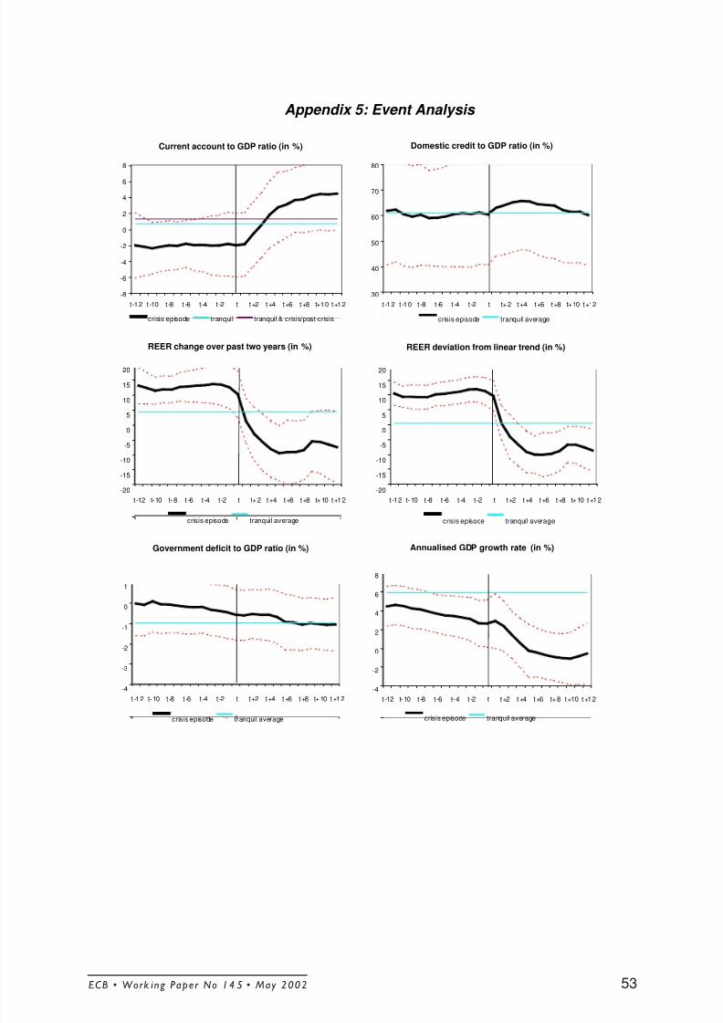
8/3/2019 Early Warning System Europe
http://slidepdf.com/reader/full/early-warning-system-europe 54/67
Appendix 5: Event Analysis
Current account to GDP ratio (in %)
-8
-6
-4
-2
0
2
4
6
8
t -12 t -10 t -8 t -6 t -4 t -2 t t+2 t+4 t+6 t+8 t+10 t+12
crisis episode tranquil tranquil & crisis/post-crisis
Domestic credit to GDP ratio (in %)
30
40
50
60
70
80
t -12 t -10 t -8 t -6 t -4 t -2 t t+2 t+4 t+6 t+8 t+10 t+12
crisis episode tranquil average
REER change over past two years (in %)
-20
-15
-10
-5
0
5
10
15
20
t -12 t-10 t-8 t -6 t -4 t -2 t t+2 t+4 t+6 t+8 t+10 t+12
crisis episode tranquil average
REER deviation from linear trend (in %)
-20
-15
-10
-5
0
5
10
15
20
t -12 t-10 t -8 t -6 t -4 t -2 t t+2 t+4 t+6 t+8 t+10 t+12
crisis episode tranquil average
Government deficit to GDP ratio (in %)
-4
-3
-2
-1
0
1
t -12 t-10 t -8 t -6 t -4 t -2 t t+2 t+4 t+6 t+8 t+10 t+12
crisis episode tranquil average
Annualised GDP growth rate (in %)
-4
-2
0
2
4
6
8
t -12 t-10 t -8 t -6 t-4 t -2 t t+2 t+4 t+6 t+8 t+10 t+12
crisis episode tranquil average
ECB • Work ing Paper No 14 5 • May 2002 53
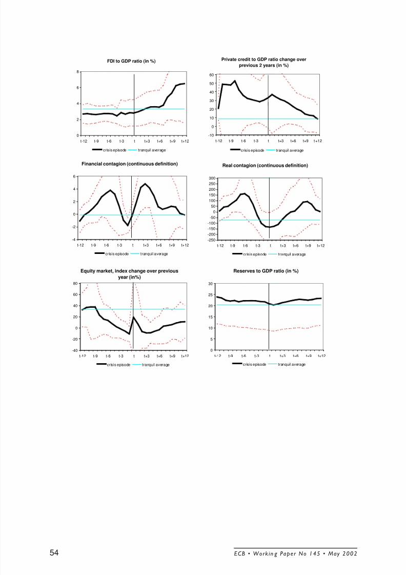
8/3/2019 Early Warning System Europe
http://slidepdf.com/reader/full/early-warning-system-europe 55/67
Financial contagion (continuous definition)
-4
-2
0
2
4
6
t-12 t-9 t-6 t-3 t t+3 t+6 t+9 t+12
crisis episode tranquil average
Real contagion (continuous definition)
-250
-200
-150
-100
-50
0
50100
150
200
250
300
t-12 t-9 t-6 t-3 t t+3 t+6 t+9 t+12
crisis episode tranquil average
Equity market, index change over previous
year (in%)
-40
-20
0
20
40
60
80
t-12 t-9 t-6 t-3 t t+3 t+6 t+9 t+12
crisis episode tranquil average
Reserves to GDP ratio (in %)
0
5
10
15
20
25
30
t-12 t-9 t-6 t-3 t t+3 t+6 t+9 t+12
crisis episode tranquil average
FDI to GDP ratio (in %)
0
2
4
6
8
t-12 t-9 t-6 t-3 t t+3 t+6 t+9 t+12
crisis episode tranquil average
Private credit to GDP ratio change over
previous 2 years (in %)
-10
0
10
20
30
40
50
60
t-12 t-9 t-6 t-3 t t+3 t+6 t+9 t+12
crisis episode tranquil average
ECB • Work in g Paper No 145 • May 200254
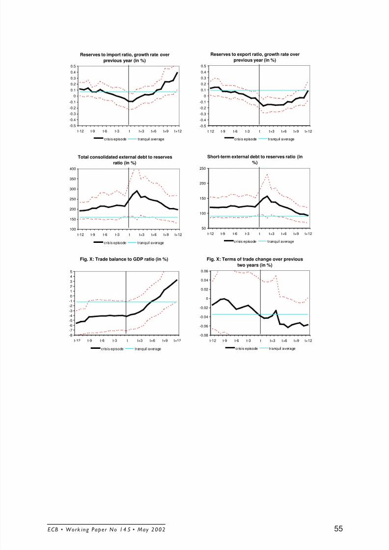
8/3/2019 Early Warning System Europe
http://slidepdf.com/reader/full/early-warning-system-europe 56/67
Reserves to export ratio, growth rate over
previous year (in %)
-0.5
-0.4
-0.3
-0.2
-0.10
0.1
0.2
0.3
0.4
0.5
t-12 t-9 t-6 t-3 t t+3 t+6 t+9 t+12
crisis episode tranquil average
Reserves to import ratio, growth rate over
previous year (in %)
-0.5
-0.4
-0.3
-0.2
-0.10
0.1
0.2
0.3
0.4
0.5
t-12 t-9 t-6 t-3 t t+3 t+6 t+9 t+12
crisis episode tranquil average
Short-term external debt to reserves ratio (in
%)
50
100
150
200
250
t-12 t-9 t-6 t-3 t t+3 t+6 t+9 t+12
crisis episode tranquil average
Total consolidated external debt to reserves
ratio (in %)
100
150
200
250
300
350
400
t-12 t-9 t-6 t-3 t t+3 t+6 t+9 t+12
crisis episode tranquil average
Fig. X: Trade balance to GDP ratio (in %)
-8
-7
-6
-5
-4
-3
-2
-1
0
1
2
3
4
5
t-12 t-9 t-6 t-3 t t+3 t+6 t+9 t+12
crisis episode tranquil average
Fig. X: Terms of trade change over previous
two years (in %)
-0.08
-0.06
-0.04
-0.02
0
0.02
0.04
0.06
t-12 t-9 t-6 t-3 t t+3 t+6 t+9 t+12
crisis episode tranquil average
ECB • Work ing Paper No 14 5 • May 2002 55
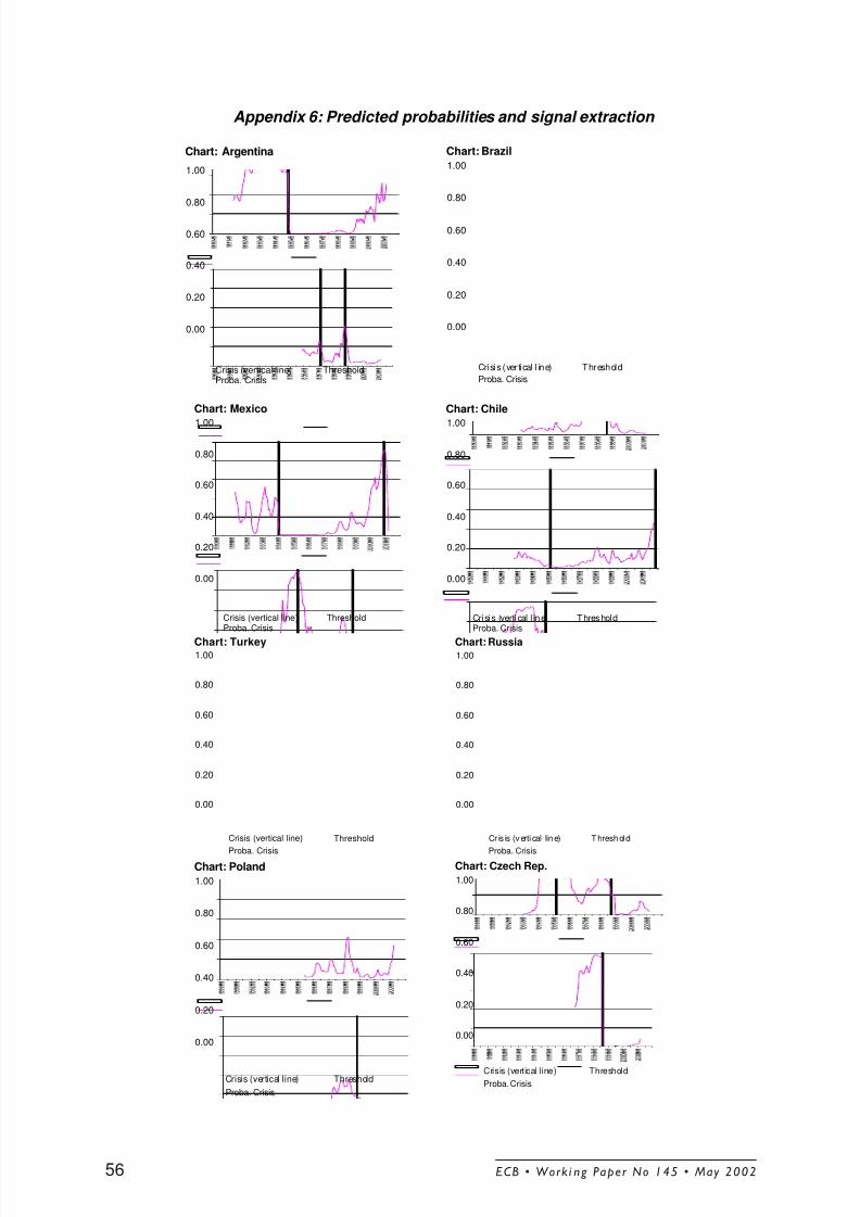
8/3/2019 Early Warning System Europe
http://slidepdf.com/reader/full/early-warning-system-europe 57/67
Appendix 6: Predicted probabilities and signal extraction
0.00
0.20
0.40
0.60
0.80
1.00
Crisis (ver tical l ine) Threshold
Proba. Crisis
Chart: Brazil
0.00
0.20
0.40
0.60
0.80
1.00
Crisis (vertical line) ThresholdProba. Crisis
Chart: Mexico
0.00
0.20
0.40
0.60
0.80
1.00
Crisis (vertical line) Threshold
Proba. Crisis
Chart: Turkey
0.00
0.20
0.40
0.60
0.80
1.00
Cr is is (verti cal line) Threshold
Proba. Crisis
Chart: Russia
0.00
0.20
0.40
0.60
0.80
1.00
Crisis (vertical line) Threshold
Proba. Crisis
Chart: Czech Rep.
0.00
0.20
0.40
0.60
0.80
1.00
Crisis (vertical line) Threshold
Proba. Crisis
Chart: Poland
0.00
0.20
0.40
0.60
0.80
1.00
Crisis (verti cal l ine) ThresholdProba. Crisis
Chart: Chile
0.00
0.20
0.40
0.60
0.80
1.00
Crisis (vertical line) ThresholdProba. Crisis
Chart: Argentina
ECB • Work i ng Paper No 145 • May 200256
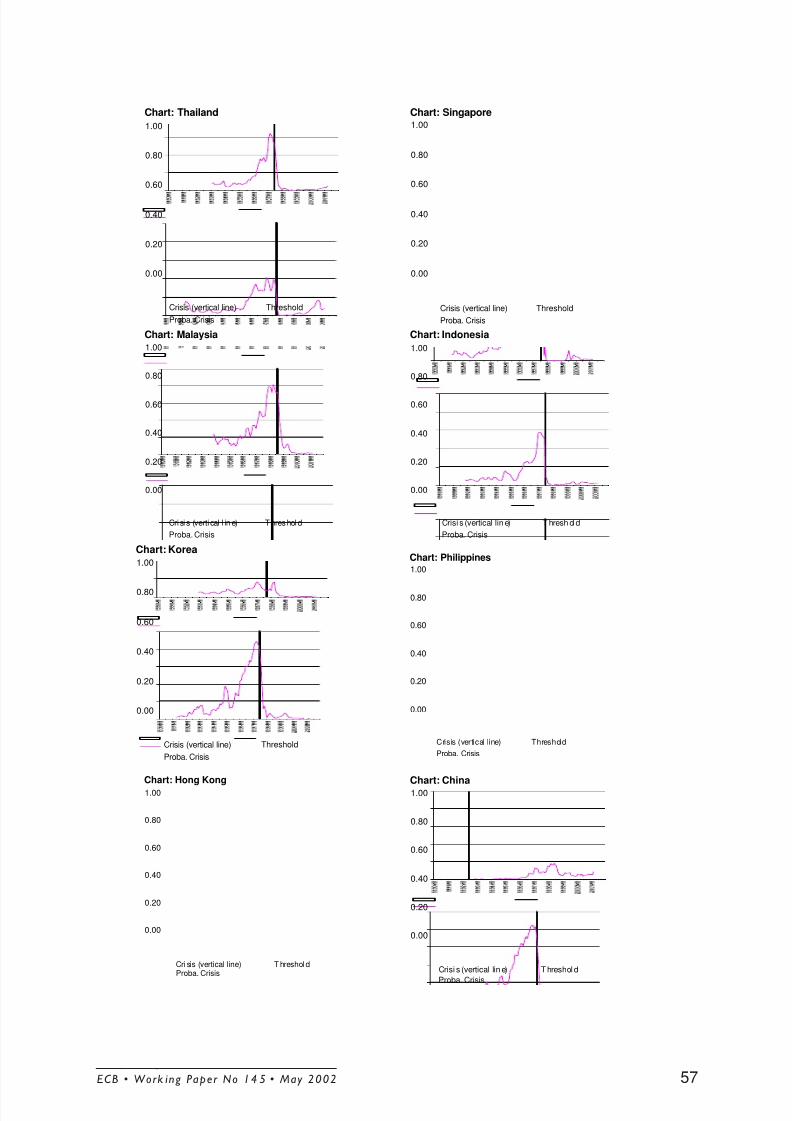
8/3/2019 Early Warning System Europe
http://slidepdf.com/reader/full/early-warning-system-europe 58/67
0.00
0.20
0.40
0.60
0.80
1.00
Crisis (vertical line) Threshold
Proba. Crisis
Chart: Thailand
0.00
0.20
0.40
0.60
0.80
1.00
Crisis (vertical line) Threshold
Proba. Crisis
Chart: Singapore
0.00
0.20
0.40
0.60
0.80
1.00
Crisis (verti cal l ine) Threshold
Proba. Crisis
Chart: Malaysia
0.00
0.20
0.40
0.60
0.80
1.00
Crisi s (vertical lin e) T hresh ol d
Proba. Crisis
Chart: Indonesia
0.00
0.20
0.40
0.60
0.80
1.00
Crisi s (vertical lin e) T hreshol d
Proba. Crisis
Chart: China
0.00
0.20
0.40
0.60
0.80
1.00
Crisis (vertical line) Threshold
Proba. Crisis
Chart: Philippines
0.00
0.20
0.40
0.60
0.80
1.00
Cri sis (vertical line) T hreshol dProba. Crisis
Chart: Hong Kong
0.00
0.20
0.40
0.60
0.80
1.00
Crisis (vertical line) Threshold
Proba. Crisis
Chart: Korea
ECB • Work ing Paper No 14 5 • May 2002 57
8/3/2019 Early Warning System Europe
http://slidepdf.com/reader/full/early-warning-system-europe 59/67
European Central Bank Working Paper Series
1 “A global hazard index for the world foreign exchange markets” by V. Brousseau and F.
Scacciavillani, May 1999.
2 “What does the single monetary policy do? A SVAR benchmark for the European Central
Bank” by C. Monticelli and O. Tristani, May 1999.
3 “Fiscal policy effectiveness and neutrality results in a non-Ricardian world” by C. Detken,
May 1999.
4 “From the ERM to the euro: new evidence on economic and policy convergence among EU
countries” by I. Angeloni and L. Dedola, May 1999.
5 “Core inflation: a review of some conceptual issues” by M. Wynne, May 1999.
6 “The demand for M3 in the euro area” by G. Coenen and J.-L. Vega, September 1999.
7 “A cross-country comparison of market structures in European banking” by O. de Bandt
and E. P. Davis, September 1999.
8 “Inflation zone targeting” by A. Orphanides and V. Wieland, October 1999.
9 “Asymptotic confidence bands for the estimated autocovariance and autocorrelation
functions of vector autoregressive models” by G. Coenen, January 2000.
10 “On the effectiveness of sterilized foreign exchange intervention” by R. Fatum,
February 2000.
11 “Is the yield curve a useful information variable for the Eurosystem?” by J. M. Berk and
P. van Bergeijk, February 2000.
12 “Indicator variables for optimal policy” by L. E. O. Svensson and M. Woodford,
February 2000.
13 “Monetary policy with uncertain parameters” by U. Söderström, February 2000.
14 “Assessing nominal income rules for monetary policy with model and data uncertainty” by
G. D. Rudebusch, February 2000.
15 “The quest for prosperity without inflation” by A. Orphanides, March 2000.
16 “Estimating the implied distribution of the future short term interest rate using the
Longstaff-Schwartz model” by P. Hördahl, March 2000.
17 “Alternative measures of the NAIRU in the euro area: estimates and assessment” by S.
Fabiani and R. Mestre, March 2000.
18 “House prices and the macroeconomy in Europe: Results from a structural VAR analysis”
by M. Iacoviello, April 2000.
ECB • Work in g Paper No 145 • May 200258
8/3/2019 Early Warning System Europe
http://slidepdf.com/reader/full/early-warning-system-europe 60/67
8/3/2019 Early Warning System Europe
http://slidepdf.com/reader/full/early-warning-system-europe 61/67
38 “The optimal inflation tax when taxes are costly to collect” by F. De Fiore,
November 2000.
39 “A money demand system for euro area M3” by C. Brand and N. Cassola,
November 2000.
40 “Financial structure and the interest rate channel of ECB monetary policy” by B. Mojon,
November 2000.
41 “Why adopt transparency? The publication of central bank forecasts” by P. M. Geraats,
January 2001.
42 “An area-wide model (AWM) for the euro area” by G. Fagan, J. Henry and R. Mestre,
January 2001.
43 “Sources of economic renewal: from the traditional firm to the knowledge firm” by
D. R. Palenzuela, February 2001.
44 “The supply and demand for eurosystem deposits – The first 18 months” by U. Bindseil
and F. Seitz, February 2001.
45 “Testing the Rank of the Hankel matrix: a statistical approach” by G. Camba-Mendez and
G. Kapetanios, February 2001.
46 “A two-factor model of the German term structure of interest rates” by N. Cassola and
J. B. Luís, February 2001.
47 “Deposit insurance and moral hazard: does the counterfactual matter?” by R. Gropp and
J. Vesala, February 2001.
48 “Financial market integration in Europe: on the effects of EMU on stock markets” by
M. Fratzscher, March 2001.
49 “Business cycle and monetary policy analysis in a structural sticky-price model of the euro
area” by M. Casares, March 2001.
50 “Employment and productivity growth in service and manufacturing sectors in France,
Germany and the US” by T. von Wachter, March 2001.
51 “The functional form of the demand for euro area M1” by L. Stracca, March 2001.
52 “Are the effects of monetary policy in the euro area greater in recessions than in booms?”
by G. Peersman and F. Smets, March 2001.
53 “An evaluation of some measures of core inflation for the euro area” by J.-L. Vega and
M. A. Wynne, April 2001.
54 “Assessment criteria for output gap estimates” by G. Camba-Méndez and D. R. Palenzuela,
April 2001.
ECB • Work in g Paper No 145 • May 200260
8/3/2019 Early Warning System Europe
http://slidepdf.com/reader/full/early-warning-system-europe 62/67
55 “Modelling the demand for loans to the private sector in the euro area” by A. Calza,
G. Gartner and J. Sousa, April 2001.
56 “Stabilization policy in a two country model and the role of financial frictions” by E. Faia,
April 2001.
57 “Model-based indicators of labour market rigidity” by S. Fabiani and D. Rodriguez-
Palenzuela, April 2001.
58 “Business cycle asymmetries in stock returns: evidence from higher order moments and
conditional densities” by G. Perez-Quiros and A. Timmermann, April 2001.
59 “Uncertain potential output: implications for monetary policy” by M. Ehrmann and
F. Smets, April 2001.
60 “A multi-country trend indicator for euro area inflation: computation and properties” by
E. Angelini, J. Henry and R. Mestre, April 2001.
61 “Diffusion index-based inflation forecasts for the euro area” by E. Angelini, J. Henry and
R. Mestre, April 2001.
62 “Spectral based methods to identify common trends and common cycles” by G. C. Mendez
and G. Kapetanios, April 2001.
63 “Does money lead inflation in the euro area?” by S. N. Altimari, May 2001.
64 “Exchange rate volatility and euro area imports” by R. Anderton and F. Skudelny,
May 2001.
65 “A system approach for measuring the euro area NAIRU” by S. Fabiani and R. Mestre,
May 2001.
66 “Can short-term foreign exchange volatility be predicted by the Global Hazard Index?” by
V. Brousseau and F. Scacciavillani, June 2001.
67 “The daily market for funds in Europe: Has something changed with the EMU?” by
G. P. Quiros and H. R. Mendizabal, June 2001.
68 “The performance of forecast-based monetary policy rules under model uncertainty” by
A. Levin, V. Wieland and J. C.Williams, July 2001.
69 “The ECB monetary policy strategy and the money market” by V. Gaspar, G. Perez-Quiros
and J. Sicilia, July 2001.
70 “Central Bank forecasts of liquidity factors: Quality, publication and the control of the
overnight rate” by U. Bindseil, July 2001.
71 “Asset market linkages in crisis periods” by P. Hartmann, S. Straetmans and C. G. de Vries,
July 2001.
72 “Bank concentration and retail interest rates” by S. Corvoisier and R. Gropp, July 2001.
ECB • Work ing Paper No 14 5 • May 2002 61
8/3/2019 Early Warning System Europe
http://slidepdf.com/reader/full/early-warning-system-europe 63/67
73 “Interbank lending and monetary policy transmission – evidence for Germany” by
M. Ehrmann and A. Worms, July 2001.
74 “Interbank market integration under asymmetric information” by X. Freixas and
C. Holthausen, August 2001.
75 “Value at risk models in finance” by S. Manganelli and R. F. Engle, August 2001.
76 “Rating agency actions and the pricing of debt and equity of European banks: What can we
infer about private sector monitoring of bank soundness?” by R. Gropp and A. J. Richards,
August 2001.
77 “Cyclically adjusted budget balances: An alternative approach” by C. Bouthevillain, P. Cour-
Thimann, G. van den Dool, P. Hernández de Cos, G. Langenus, M. Mohr, S. Momigliano
and M. Tujula, September 2001.
78 “Investment and monetary policy in the euro area” by B. Mojon, F. Smets andP. Vermeulen, September 2001.
79 “Does liquidity matter? Properties of a synthetic divisia monetary aggregate in the euro
area” by L. Stracca, October 2001.
80 “The microstructure of the euro money market” by P. Hartmann, M. Manna and
A. Manzanares, October 2001.
81 “What can changes in structural factors tell us about unemployment in Europe?” by
J. Morgan and A. Mourougane, October 2001.
82 “Economic forecasting: some lessons from recent research” by D. Hendry and
M. Clements, October 2001.
83 “Chi-squared tests of interval and density forecasts, and the Bank of England's fan charts”
by K. F. Wallis, November 2001.
84 “Data uncertainty and the role of money as an information variable for monetary policy” by
G. Coenen, A. Levin and V. Wieland, November 2001.
85 “Determinants of the euro real effective exchange rate: a BEER/PEER approach” by
F. Maeso-Fernandez, C. Osbat and B. Schnatz, November 2001. 86 “Rational expectations and near rational alternatives: how best to form expecations” by
M. Beeby, S. G. Hall and S. B. Henry, November 2001. 87 “Credit rationing, output gap and business cycles” by F. Boissay, November 2001. 88 “Why is it so difficult to beat the random walk forecast of exchange rates?” by L. Kilian and
M. P. Taylor, November 2001.
ECB • Work in g Paper No 145 • May 200262
8/3/2019 Early Warning System Europe
http://slidepdf.com/reader/full/early-warning-system-europe 64/67
89 “Monetary policy and fears of financial instability” by V. Brousseau and C. Detken,
November 2001.
90 “Public pensions and growth” by S. Lambrecht, P. Michel and J.-P. Vidal, November 2001.
91 “The monetary transmission mechanism in the euro area: more evidence from VAR
analysis” by G. Peersman and F. Smets, December 2001.
92 “A VAR description of the effects of monetary policy in the individual countries of the euro
area” by B. Mojon and G. Peersman, December 2001.
93 “The monetary transmission mechanism at the euro-area level: issues and results using
structural macroeconomic models” by P. McAdam and J. Morgan, December 2001.
94 “Monetary policy transmission in the euro area: what do aggregate and national structural
models tell us?” by P. van Els, A. Locarno, J. Morgan and J.-P. Villetelle, December 2001.
95 “Some stylised facts on the euro area business cycle” by A.-M. Agresti and B. Mojon,December 2001.
96 “The reaction of bank lending to monetary policy measures in Germany” by A. Worms,
December 2001.
97 “Asymmetries in bank lending behaviour. Austria during the 1990s” by S. Kaufmann,
December 2001.
98 “The credit channel in the Netherlands: evidence from bank balance sheets” by L. De Haan,
December 2001.
99 “Is there a bank lending channel of monetary policy in Spain?” by I. Hernando and
J. Martínez-Pagés, December 2001.
100 “Transmission of monetary policy shocks in Finland: evidence from bank level data on
loans” by J. Topi and J. Vilmunen, December 2001.
101 “Monetary policy and bank lending in France: are there asymmetries?” by C. Loupias,
F. Savignac and P. Sevestre, December 2001.
102 “The bank lending channel of monetary policy: identification and estimation using
Portuguese micro bank data” by L. Farinha and C. Robalo Marques, December 2001.
103 “Bank-specific characteristics and monetary policy transmission: the case of Italy” by
L. Gambacorta, December 2001.
104 “Is there a bank lending channel of monetary policy in Greece? Evidence from bank level
data” by S. N. Brissimis, N. C. Kamberoglou and G. T. Simigiannis, December 2001.
105 “Financial systems and the role of banks in monetary policy transmission in the euro area”
by M. Ehrmann, L. Gambacorta, J . Martínez-Pagés, P. Sevestre and A. Worms,
December 2001.
ECB • Work ing Paper No 14 5 • May 2002 63
8/3/2019 Early Warning System Europe
http://slidepdf.com/reader/full/early-warning-system-europe 65/67
106 “Investment, the cost of capital, and monetary policy in the nineties in France: a panel data
investigation” by J.-B. Chatelain and A. Tiomo, December 2001.
107 “The interest rate and credit channel in Belgium: an investigation with micro-level firm
data” by P. Butzen, C. Fuss and P. Vermeulen, December 2001.
108 “Credit channel and investment behaviour in Austria: a micro-econometric approach” by
M. Valderrama, December 2001.
109 “Monetary transmission in Germany: new perspectives on financial constraints and
investment spending” by U. von Kalckreuth, December 2001.
110 “Does monetary policy have asymmetric effects? A look at the investment decisions of
Italian firms” by E. Gaiotti and A. Generale, December 2001.
111 “Monetary transmission: empirical evidence from Luxembourg firm level data” by
P. Lünnemann and T. Mathä, December 2001.
112 “Firm investment and monetary transmission in the euro area” by J.-B. Chatelain,
A. Generale, I. Hernando, U. von Kalckreuth and P. Vermeulen, December 2001.
113 “Financial frictions and the monetary transmission mechanism: theory, evidence and policy
implications” by C. Bean, J. Larsen and K. Nikolov, January 2002.
114 “Monetary transmission in the euro area: where do we stand?” by I. Angeloni, A. Kashyap,
B. Mojon, D. Terlizzese, January 2002.
115 “Monetary policy rules, macroeconomic stability and inflation: a view from the trenches”
by A. Orphanides, December 2001.
116 “Rent indices for housing in West Germany 1985 to 1998” by J. Hoffmann and C. Kurz.,
January 2002.
117 “Hedonic house prices without characteristics: the case of new multiunit housing” by
O. Bover and P. Velilla, January 2002.
118 “Durable goods, price indexes and quality change: an application to automobile prices in
Italy, 1988-1998” by G. M. Tomat, January 2002.
119 “Monetary policy and the stock market in the euro area” by N. Cassola and C. Morana,
January 2002.
120 “Learning stability in economics with heterogenous agents” by S. Honkapohja and K. Mitra,
January 2002.
121 “Natural rate doubts” by A. Beyer and R. E. A. Farmer, February 2002.
122 “New technologies and productivity growth in the euro area” by F. Vijselaar and R. Albers,
February 2002.
ECB • Work in g Paper No 145 • May 200264
8/3/2019 Early Warning System Europe
http://slidepdf.com/reader/full/early-warning-system-europe 66/67
123 “Analysing and combining multiple credit assessments of financial institutions” by E. Tabakis
and A. Vinci, February 2002.
124 “Monetary policy, expectations and commitment” by G. W. Evans and S. Honkapohja,
February 2002.
125 “Duration, volume and volatility impact of trades” by S. Manganelli, February 2002.
126 “Optimal contracts in a dynamic costly state verification model” by C. Monnet and
E. Quintin, February 2002.
127 “Performance of monetary policy with internal central bank forecasting” by S. Honkapohja
and K. Mitra, February 2002.
128 “Openness, imperfect exchange rate pass-through and monetary policy” by F. Smets and
R. Wouters, February 2002.
129 “Non-standard central bank loss functions, skewed risks, and certainty equivalence” by
A. al-Nowaihi and L. Stracca, March 2002.
130 “Harmonized indexes of consumer prices: their conceptual foundations” by E. Diewert,
March 2002.
131 “Measurement bias in the HICP: what do we know, and what do we need to know?” by
M. A. Wynne and D. Rodríguez-Palenzuela, March 2002.
132 “Inflation dynamics and dual inflation in accession countries: a “new Keynesian”
perspective” by O. Arratibel, D. Rodríguez-Palenzuela and C. Thimann, March 2002.
133 “Can confidence indicators be useful to predict short term real GDP growth?” by
A. Mourougane and M. Roma, March 2002.
134 “The cost of private transportation in the Netherlands, 1992-1999” by B. Bode and
J. Van Dalen, March 2002.
135 “The optimal mix of taxes on money, consumption and income” by F. De Fiore and
P. Teles, April 2002.
136 “Retail bank interest rate pass-through: the new evidence at the euro area level” by
G. de Bondt, April 2002.
137 “Equilibrium bidding in the eurosystem’s open market operations” by U. Bindseil, April
2002.
138 “New” views on the optimum currency area theory: what is EMU telling us?” by
F. P. Mongelli, April 2002.
139 “On currency crises and contagion” by M. Fratzscher, April 2002.
140 “Price setting and the steady-state effects of inflation” by M. Casares, May 2002.
ECB • Work ing Paper No 14 5 • May 2002 65

8/3/2019 Early Warning System Europe
http://slidepdf.com/reader/full/early-warning-system-europe 67/67
141 “Asset prices and fiscal balances” by F. Eschenbach and L. Schuknecht, May 2002.
142 “Modelling the daily banknotes in circulation in the context of the liquidity management of
the European Central Bank”, by A. Cabrero, G. Camba-Mendez, A. Hirsch and F. Nieto,
May 2002.
143 “A non-parametric method for measuring new goods”, by I. Crawford, May 2002.
144 “A failure in the measurement of inflation: results from a hedonic and matched experiment
using scanner data”, by M. Silver and S. Heravi, May 2002.
145 “Towards a new early warning system of financial crises”, by M. Fratzscher and M. Bussiere,
May 2002.