Dynamics of senescence-related QTLs in potato

Paula Ximena Hurtado • Sabine K. Schnabel • Alon Zaban •

Merja Vetelainen • Elina Virtanen • Paul H. C. Eilers •

Fred A. van Eeuwijk • Richard G. F. Visser • Chris Maliepaard

Received: 27 February 2010 / Accepted: 17 May 2011 / Published online: 12 June 2011

� The Author(s) 2011. This article is published with open access at Springerlink.com

Abstract The study of quantitative trait’s expression

over time helps to understand developmental processes

which occur in the course of the growing season.

Temperature and other environmental factors play an

important role. The dynamics of haulm senescence was

observed in a diploid potato mapping population in two

consecutive years (2004 and 2005) under field condi-

tions in Finland. The available time series data were

used in a smoothed generalized linear model to

characterize curves describing the senescence devel-

opment in terms of its onset, mean and maximum

progression rate and inflection point. These character-

istics together with the individual time points were

used in a Quantitative trait loci (QTL) analysis.

Although QTLs occurring early in the senescence

process coincided with QTLs for onset of senescence,

the analysis of the time points made it difficult to study

senescence as a continuous trait. Characteristics esti-

mated from the senescence curve allowed us to study it

as a developmental process and provide a meaningful

biological interpretation to the results. Stable QTLs in

the two experimental years were identified for pro-

gression rate and year-specific QTLs were detected for

onset of senescence and inflection point. Specific

interactions between loci controlling senescence

development were also found. Epistatic interaction

between QTLs on chromosomes 4, 5 and 7 were

detected in 2004 and pleiotopic effects of QTLs on

chromosomes 3 and 4 were observed in 2005.

Keywords Beta-thermal time � Epistasis �Functional QTL mapping � Smoothing �Time series � GLM

Introduction

The study of developmental processes in plants

requires the evaluation of traits over time taking into

P. X. Hurtado (&) � R. G. F. Visser � C. Maliepaard

Wageningen UR Plant Breeding, Wageningen University,

P.O. Box 386, 6700 AJ Wageningen, The Netherlands

e-mail: paula.hurtadolopez@wur.nl

P. X. Hurtado � S. K. Schnabel � P. H. C. Eilers �F. A. van Eeuwijk

Biometris—Applied Statistics, Wageningen University,

P.O. Box 100, 6700 AC Wageningen, The Netherlands

A. Zaban � M. Vetelainen � E. Virtanen

AgriFood Research Finland (MTT), North Ostrobothnia

Research Station, Ruukki, Finland

P. H. C. Eilers

Department of Biostatistics, Erasmus Medical Center,

P.O. Box 2040, 3000 CA Rotterdam, The Netherlands

P. X. Hurtado

C.T. de Wit Graduate School for Production Ecology

and Resource Conservation (PE&RC), Wageningen

University, P.O. Box 386, 6708 PB Wageningen,

The Netherlands

S. K. Schnabel � F. A. van Eeuwijk � R. G. F. Visser

Centre for BioSystems Genomics, P.O. Box 98,

6700 AB Wageningen, The Netherlands

123

Euphytica (2012) 183:289–302

DOI 10.1007/s10681-011-0464-4

account the continuous nature of development.

Quantitative traits normally involved in these pro-

cesses require assessments at several time points

during the life cycle. However, conventional exper-

iments include evaluations at a single fixed time point

during the growing season. Quantitative trait loci

(QTL) analysis using the data collected from those

experiments give just an impression of the loci

affecting the trait at a particular developmental stage.

The understanding of the genetic basis controlling

quantitative traits improves when the evolution of the

trait during the life cycle and the developmental

pattern are considered. In addition, environmental

factors affecting crop development, such as temper-

ature and photoperiod, must be also taken into

account. Therefore, growth models flexible enough

to be adapted to the usually non-linear trait responses

over time have to be implemented. Examples of

commonly used models in biology are the exponen-

tial growth models and the family of s-shaped curves

(Schnute 1981). These models have the advantage of

describing the development of the trait in terms of

curve parameters with a biological interpretation. The

differences in growth trajectories between genotypes

are reflected by genotype-specific curve parameters.

Growth models and QTL analysis can be combined

by modeling growth curve parameters in terms of

QTLs in one-step (Ma et al. 2002; Malosetti et al.

2006) or two-step model approaches (Reymond et al.

2003; Yin et al. 1995). In the former, logistic growth

curves and QTL mapping are combined, modeling

growth parameters as a function of the QTL geno-

types described by molecular marker scores. In the

latter, first genotype-specific parameters are esti-

mated from the growth curves, thereafter they are

used as phenotypic traits in a conventional QTL

analysis. In both approaches, the accurate estimation

of the curve parameters plays an important role to

find meaningful results.

In our study, haulm senescence was assessed at

several time points during the growing season on a

diploid potato mapping population evaluated for two

consecutive years in Finland (2004 and 2005). We are

presenting here an alternative two-step approach:

modeling first in a flexible way the curve trajectories

with a smoothed generalized linear model (GLM)

procedure. We used the collected time series data to

model the development of senescence in terms of time

and temperature. To allow a better comparability of the

trait across the years, we converted the calendar days

after planting into beta-thermal days after planting

(TAP) using a non-linear temperature effect function

described by Khan et al. (2011). Once the senescence

trajectory was defined, the characteristics of the curve-

such as onset, maximum and average progression rate

and inflection point- were estimated from the first and

second derivative of the curve. These characteristics

were used as phenotypic traits describing senescence

development in the QTL analysis. In this way, the

characterization of the smoothed GLM curves allowed

us to map the genetic basis of the senescence process

giving a meaningful biological interpretation to the

results.

Materials and methods

Description of the C9E potato population

The evaluation of haulm senescence was done on a

diploid backcross potato population (C9E) composed

of 250 genotypes. The C9E population is the result

of a cross between two diploid potato clones. The

female parent, the C clone US-W5337.3 (Hanneman

and Peloquin 1967) is a hybrid between Solanum

phureja (PI225696) and S. tuberosum dihaploid

US-W42. The male parent, the E clone (Jacobsen

1980), is a hybrid between VH34211 (a S. vernei–S.

tuberosum backcross) and the C clone itself.

S. phureja is characterized by a lack of dormancy,

early maturity and short day tuberization induction.

In contrast, S. tuberosum varieties have long dor-

mancy, variable maturity and long day tuberization

induction (Hawkes 1990; Ewing and Struik 1992).

The different day length requirements for tuberiza-

tion of S. phurja and S. tuberosum has provided a

source of genetic variation in the C9E population

making it suitable for the study of developmental

processes under different photoperiods.

Experimental design and description of the haulm

senescence evaluation

The very long day conditions of northern Finland

were used to conduct an experiment in two consec-

utive years (2004 and 2005) in the experimental field

of AgriFood Research Finland (MTT) at the North

Ostrobothnia Research Station in Ruukki (64�420N,

290 Euphytica (2012) 183:289–302

123

25�000E). The experiment performed in 2004 was

previously described by Zaban et al. (2006). Sets of

197 and 222 genotypes of the C9E population were

planted in plots of three plants per genotype, where

the genotypes were randomized, on June 1st 2004 and

May 16th 2005, respectively. We acknowledge that in

these trials there was no real replication of genotypes,

but only pseudo-replications. Each plant was evalu-

ated at several time points spaced in intervals of

3–7 days. In 2004 the observation period was 52 days

with evaluations at 77, 81, 86, 91, 95, 100, 105, 109,

116, 123, 129 days after planting (DAP). In the

second year the observation period was shorter

(31 days) and haulm senescence was evaluated at

84, 88, 93, 98, 101, 106, 109, 112 and 115 DAP. The

process of senescence was defined as the period

between the last observation at which the plant was

entirely green and the first date at which the plant was

dead (Celis-Gamboa 2002). The progress of the trait

was measured using the scale described by Celis-

Gamboa et al. (2003) in which 1 = green plant;

2 = upper leaves with the first signs of yellowing

(light green); 3 = yellow leaves; 4 = 25% of haulm

tissue brown; 5 = 50% of haulm tissue brown;

6 = more than 75% of haulm tissue brown; 7 = dead

plant.

Description of Beta-thermal time estimation

Crop development is mainly affected by temperature

and can be modified by other factors such as

photoperiod (Hodges 1991). Previous studies have

shown that potato growth is influenced by tempera-

ture, where warmer temperatures favor vegetative

growth accelerating reproductive and vegetative

development (Haun 1975; Benoit et al. 1986; Struik

and Ewing 1995). Whereas, lower temperatures

facilitate tuber growth (Marinus and Boadlaender

1975). The effect of temperature on crop develop-

ment rate is often described by using a thermal time

concept. Various non-linear models have been devel-

oped to describe temperature response of develop-

mental processes in plants (Johnson and Thornley

1985; Gao et al. 1992; Yin et al. 1995). In our study,

the daily contribution of temperature to plant devel-

opment in 2004 was different from 2005 due to the

fluctuations in daily air temperature. A summary of

the meteorological conditions reported by the station

in Ruukki (Finland) during the growing season in the

two experimental years is presented in Table 1. The

growing season defined as the period between the last

killing frost of spring and the first killing frost of

autumn (Allaby 1998) was defined in 2004 from

April 16 to November 10 and in 2005 from May 3 to

November 14. To allow for a better comparability of

senescence across the years, we converted the

calendar DAP into beta-thermal days after planting

(TAP) using the non-linear temperature effect func-

tion g(T) described by Khan et al. (2011):

gðTÞ ¼ Tc � T

Tc � To

� �T � Tb

To � Tb

� �To�TbTc�To

" #ct

ð1Þ

where the three main temperatures, base, optimum

and ceiling temperature for phenological develop-

ment of potato, were defined as Tb = 5.5�C,

To = 23.4�C and Tc = 34.6�C, respectively. The

temperature response curvature coefficient was esti-

mated as ct = 1.7 according to Khan et al. (2011).

Because the function g(T) is non-linear and temper-

ature fluctuates daily, g(T) was estimated using the

average daily air temperature to obtain the daily

value. The cumulative TAP, combining temperature

and time (beta-thermal time, BTT), was the scale of

the x-axis used to compare senescence development

in the two experimental years.

Table 1 Summary of meteorological conditions reported in Ruukki, Finland during the growing season in 2004 and 2005

Year 2004 2005

Average daily air temperature (�C) 12.7 14.5

Temperature range (�C) 2.6–20.5 4.8–21.9

Amount of rainfall (mm) 514 359

Average daily rainfall (mm) 2.1 1.5

Average daily radiation (kJ/cm2) 142.9 155.05

Radiation range (kJ/cm2) 19.20–297.20 35.04–280.72

Euphytica (2012) 183:289–302 291

123

Description of the smoothed generalized linear

model procedure

To estimate the senescence curve non-parametrically,

a variant of penalized B-splines, P-splines (Eilers and

Marx 1996), was used. Then we interpreted a senes-

cence value y as having observed y ‘‘successes’’ in n

binomial trials and we estimated a smooth curve for the

probability p of a ‘‘success’’. To guarantee that

0 \ p \ 1, we worked with the linear predictor. In

this case it is the logit, g = log(p/(1-p)), which has no

restrictions on its range. This is standard practice in

logistic regression and generalized linear models

(Nelder and Wedderburn 1972). Smooth logistic

regression with P-splines was explained by Eilers

and Marx (1996). They also showed that automatic

interpolation was obtained. We exploited this prop-

erty by working with zero degree B-splines including a

knot on each beta-thermal day (TAP units) of the

domain we study. The penalized log-likelihood in this

situation is

l� ¼X

i

wi½yi logpiþðni� yiÞ logð1� piÞþ logni

yi

� ��

� k2

Xi

ðD2giÞ2�j2

Xi

g2i ð2Þ

with pi ¼ 1= 1þ e�gið Þ:The weight is determined by

wi ¼ npi 1� pið Þ following GLM methodology for

our situation. The second term in the equation above

is the penalty on the linear predictor g. The parameter

k tunes its weight: the larger k, the smoother the

result. We used the operator notation to indicate

repeated differences: D2gi ¼ gi� 2gi�1 þ gi�2 ¼gi� gi�1ð Þ� gi�1� gi�2ð Þ:

One can show that for very large k the estimated

curve for p approaches the logistic curve. Further-

more we used a ridge penalty on g tuned by the

parameter j to avoid numerical instabilities, when gbecomes too large. To estimate g, the iterative

weighted linear regression algorithm (Nelder and

Wedderburn 1972) was modified, to account for the

penalties.

The fitting procedure resulted in a smooth curve

for the development of haulm senescence over time

for each genotype. This flexible functional form using

splines allowed to model different shapes of these

curves (e.g., for early and late genotypes) within the

same framework.

Characteristics estimated from the senescence

curves

Once the senescence curves were fitted, some charac-

teristics of the curves describing the ageing process

were estimated to allow the study of senescence as a

continuous trait changing in time. The characteristics

estimated from the curve have a meaningful biological

interpretation for the senescence development and

facilitate the understanding of the QTL mapping

results. We calculated the first differences on the curve

values (first derivative) as a proxy of the slope of the

curve. The mean slope or mean progression rate

(mprate) is reflecting the average rate of change of the

senescence curve during the whole observation period

giving an idea of how fast a genotype is experiencing

the senescence process. The maximum slope (prate)

explains the maximum rate of change of the senescence

curve when the plant has completed half of the

senescence process (between 4 and 5 in the senescence

scale). The higher the value, the faster full senescence

is reached during the observation period. The inflection

point (ipoint) reflects the point in time when half of the

senescence process has been reached and the trajectory

curve change from convex to concave shape indicating

the beginning of the final stage. Additional character-

istics were deduced from the second differences of the

curve values (second derivative), including the max-

imum and minimum change of the slope, which are

interpreted as the onset and the end of the senescence

process. The onset is indicating the beginning of the

senescence process in terms of time or more accurately

in our case in terms of BTT. The lower the value, the

earlier the senescence process starts.

Repeatability estimation

Data from the three plants within a plot for individual

genotypes were used for a repeatability estimation,

calculated for each year. The repeatability was

defined by the ratio of genetic (genotypic) to

phenotypic variance. Phenotypic variance was equal

to the sum of the genetic variance and a third times

the between-plants-within-plot variance.

G9E interactions

The estimation of genotype by year interactions

included 186 genotypes evaluated in the two

292 Euphytica (2012) 183:289–302

123

consecutive years using a two-way analysis of

variance with genotype and environment fixed in

the model. The curve characteristics (mprate, prate,

ipoint and onset) were used as response variables, y,

and the genotype (G), year (E) and Genotype 9 Year

(G 9 E) interaction as the explanatory variables in

the model, which also includes an error term (based

on the variation between the three plants per

genotype):

y ¼ Gþ E þ G� E þ error: ð3Þ

Description of the genetic map and molecular data

The C9E population was genotyped using amplified

fragment length polymorphism, AFLP (Celis-Gam-

boa 2002), simple sequence repeat, SSR, and cleav-

age amplified polymorphism, CAPS (Werij et al.

2007). Our study included a subset of dominant and

co-dominant markers with the expected segregation

ratios 1:1 and 1:1:1:1, respectively. JoinMap 4 (Van

Ooijen 2006) was used to construct the C and E

parental maps using 164 and 198 markers, respec-

tively, each with 12 linkage groups (LG) previously

reported by Celis-Gamboa (2002). The C map

consisted of 135 markers spanning 917.4 cM. Four

of the 12 LG were split in two sub-groups and one

was split in 3 sub-groups due to the large distances

between adjacent markers (more than 30 cM). The E

map consisted of 132 markers spanning 629.8 cM

and 2 of the 12 LG were split in 2 sub-groups. Since

the maternal (C) and paternal (E) maps were not

integrated due to the expected differences in the

recombination frequencies between the two parents

(with genetic background from two different Solanum

species), the separated parental maps were used to

perform the QTL analysis. Co-dominant markers

present in both parental maps (C and E) were used to

identify the same LG in the two maps. The assign-

ment of linkage groups was done using as a reference

the maps of Celis-Gamboa (2002), each LG is

preceded by the letter C or E according to the

parental map, followed by the LG number.

QTL analysis using curve characteristics

and single time points

The detection of QTLs, estimation of QTL main

effects and their interactions was done in two steps.

In the first step, the detection of QTLs was performed

separately for each type of phenotypic data available.

In the analysis per time point the senescence scores,

from 1 to 7, were used in the QTL mapping. In the

analysis of the characteristics estimated from the

curves (mprate, prate, ipoint and onset), each char-

acteristic was used as a quantitative trait. The use of

model parameters in QTL mapping has been intro-

duced in functional mapping for the analysis of time-

series traits. It incorporates biological principles

(defined with mathematical functions) into the frame-

work for QTL mapping (Wu et al. 2003; Wu and Lin

2006).

A nonparametric QTL analysis was performed for

the time point data using the rank sum test of

Kruskal–Wallis (KW). The curve characteristics were

analyzed using both KW and interval mapping (IM).

Both procedures are available in MapQTL 6 (Van

Ooijen 2009). For the curve characteristics, QTLs

detected by KW and IM were the same. For

transparent comparison of QTL analysis on time

points and curve characteristics, in this paper we

present only results from KW.

QTL mapping was performed separately on the

parental maps and the criterion for detecting QTLs

was set at a significance level of P B 0.005 (Van

Ooijen 2006). To identify the detected QTLs, the

origin of the map (C and E parent) and the linkage

group are indicated in the QTL name using italic

letters. The QTLs were named according to the

parental map and the linkage group in which they

were identified. As an example, the most significant

QTL on linkage group 4 in the C parent was called

C4 and in the case of common markers detected in

both parents, like E5 and C5, the QTL was called Ch5

(corresponding to a QTL on chromosome 5).

QTL 9 QTL interactions

IM was used for detecting main effect QTLs for the

curve characteristics mprate, prate, ipoint and onset.

The presence of epistatic interactions was investigated

per year by fitting linear models (Genstat release 13.2,

Payne et al. 2010) containing pairwise interactions

between those QTLs for whom earlier main effects

were detected for any of the four curve characteristics.

A full model was defined with each curve character-

istic as response variable, y, and the main effect QTLs

Euphytica (2012) 183:289–302 293

123

together with all possible QTL 9 QTL interactions as

fixed explanatory variables.

y ¼ QTLsþ QTL� QTL interactionsþ error ð4ÞFrom the full model (4), for each curve character-

istic a subset of model terms was created. This list

contained the significant main effects QTLs, all

significant epistatic interactions, plus non-significant

main effect QTLs whenever these QTLs were

involved in significant epistatic interactions. A final

model was fitted for each curve characteristic

including only the earlier selected terms.

Results

Curve fitting

The transformation of normal calendar days after

planting into TAP and their cumulative values gener-

ated a new scale (BTT) to measure the senescence

development in terms of time and accumulated tem-

perature. BTT went from 33.3 to 41.85 and from 37.1 to

50.8 during the observation period in 2004 (77–129

DAP) and 2005 (84–115 DAP), respectively. This

scale was used as the x-axis to fit the curves and

visualize the progression of haulm senescence scored

from 1 to 7. The use of the smoothed GLM procedure in

our study allowed flexible modeling of different curve

shapes. Different types of curves were observed in the

C9E population according to the maturity type of each

genotype (Fig. 1a). The description of the five catego-

ries (very early, early, intermediate, late and very late)

according to the duration of the plant cycle was

reported by Celis-Gamboa (2002). In early genotypes

we observed a logistic s-shape in the curve trajectory

while in the late genotypes we had only the exponential

part of the curves often corresponding to completion of

only about half of the senescence process.

After fitting the curves for each genotype, several

characteristics describing the ageing process were

estimated to be used in the QTL analysis. The first

differences on the curves allowed the estimation of

mprate, prate and ipoint (Fig. 1b) and the second

derivative was used to determine the onset of the

senescence process (Fig. 1c). The minimum second

derivative was calculated for the early and interme-

diate genotypes but it was not accurately estimated

for the late genotypes, therefore it was not considered

in this study. However, it can be interpreted as the

end of the senescence process and experiments with a

longer observation period could make use of this

characteristic as well to describe the final stage of

senescence.

Repeatability estimation

Once the curve characteristics were calculated, the

repeatability of each one was estimated for each year.

Fig. 1 Characterization of senescence development in the

C9E population represented by three genotypes with different

maturity type: CE78 (early: red-top line), CE47 (intermediate:

blue-middle line) and CE697 (late: yellow-lowest line). a Fitted

curves showing the senescence development. b First derivative

of the curves in which the maximum slope represents the

progression rate and the dashed lines represent the time when

half of the senescence process has been completed (inflection

point) in each genotype. c Second derivative of the curves in

which the maximum second difference is interpreted as the

onset of senescence and it is indicated with a dashed line in

each genotype. BTT beta-thermal time representing cumulative

TAP beta-thermal days after planting

294 Euphytica (2012) 183:289–302

123

High values were observed for all of them in the

2 years with values between 0.89 and 0.98. Repeat-

ability was also estimated in each time point and

values higher than 0.92 were obtained during the

observation period in each year. The high repeatabil-

ity values observed in the curve characteristics and in

the individual time points are due to the experimental

design.

G9E interactions

A set of 186 genotypes evaluated in 2004 and 2005

was used to estimate the year effect, the genotype

main effect and G9E interaction for prate, mprate,

ipoint and onset according to model (3). There was a

clear year effect for all four traits (P \ 0.001). We

observed in 2005 a senescence period lasting longer

than in 2004 with a slow progression rate. In 2004,

the average mprate and prate were higher (0.36 and

0.86) than in 2005 (0.24 and 0.55), whereas the

average onset and ipoint were higher in 2005 (45.97

and 49.90) than in 2004 (37.28 and 39.65). The

observation period in 2005 was not long enough for

late genotypes to complete the senescence process.

Figure 2 shows the senescence fitted curves of three

genotypes with different maturity type (CE78: early,

CE47: intermediate and CE697: late) in 2004 and

2005 to exemplify the effect of genotype and year in

the C9E population. Significant interactions between

genotypes and year (P-value \ 0.001) were also

observed for each curve characteristic. Larger differ-

ences in mprate, ipoint and onset were observed

between early and late genotypes in 2005, whereas

the differences between early and late genotypes

were larger for prate in 2004. Early genotypes had a

fast senescence development and late genotypes

became very late in 2005.

QTL analysis: characteristics of the curves

and single time points

QTLs were detected in each parental map using the

individual time points and the characteristics esti-

mated from the curves in each year, considering as a

significance threshold a P-value from the Kruskal–

Wallis test lower than 0.005. Only the LGs in which

QTLs were identified are shown in Fig. 3 and two

levels of significance are highlighted (0.001 \ P B

0.005, P B 0.001). In the analysis per time point, 10

and 9 time points were used in the QTL analysis in

2004 and 2005, respectively. In the first year, the first

time point was excluded from the analysis because all

the genotypes were still green. In the analysis using

the curve characteristics, although four of them were

used for the QTL mapping using KW and IM, results

are presented only for onset, prate and ipoint with

Kruskal–Wallis. It is due to the fact that high

correlations were observed between mprate and prate

in the two consecutive years (0.85 and 0.80, respec-

tively) and the same QTLs were detected for both

curve characteristics using KW and IM.

Comparing the results using time points and curve

characteristics, we observed that QTLs detected in

early time points, coincided with QTLs on LG C4,

C5A and E3 associated with onset of senescence.

QTLs occurring in more advanced stages of the

senescence development coincided with QTLs for

prate and ipoint as shown in C5 and E5 (they

correspond to the same LG in both parents and hence

are termed Ch5).

Environment (year)-specific QTLs were found on

C1 and C5A associated with prate in 2005 and onset

in 2004, respectively. QTLs associated with ipoint

were also related with onset in 2005 as it is shown in

E7 and Ch5. The pleiotropic QTLs detected for ipoint

and onset on both LG explained the high correlation

(0.8) observed between the two traits in that year. On

the other hand, QTLs consistently found in C4 in the

two experimental years were associated with onset

and the more significant P-value was observed in

2005 (P \ 0.0001).

Fig. 2 Comparison of senescence development in Finland

during 2004 (solid line) and 2005 (dashed line) represented by

three genotypes with different maturity type: CE78 (early: red-

top line), CE47 (intermediate: blue-middle line) and CE697

(late: yellow-lowest line). The x-axis corresponds to BTT units

adjusted for comparison of the 2 years

Euphytica (2012) 183:289–302 295

123

a

296 Euphytica (2012) 183:289–302

123

QTL9QTL interactions

The most significant QTLs for prate, ipoint and onset

in each linkage group and all the pairwise interactions

between them were used in a linear model to investi-

gate epistatic interactions, within a year. The full

model was based on the joined set of main effect QTLs

as detected for any of the three curve characteristics.

Fig. 3 Graphical representation of the QTLs detected in the C

(a) and E (b) parental maps. Results from the QTL analysis using

data from the field experiments in 2004 and 2005 are presented in

the left and right panel respectively. Only the linkage groups in

which significant QTLs were detected using individual time

points (in 2004: 81,86,91,95,100,105,109,116,123 and 129DAP;

in 2005:84,88,93,98,101,106,109,112 and 115 DAP) and curve

characteristics (onset, ipoint, prate) are presented. The colors in

the linkage groups indicate the significance levels (white:

P [ 0.005, yellow: 0.001 \ P B 0.005, brown: P B 0.001)

Fig. 3 continued

b

Euphytica (2012) 183:289–302 297

123

Therefore, the full model was the same for prate,

ipoint and onset and it was set according to model (4)

including only two-way interactions betweenQTLs:

y ¼E3þ Ch5þ E7 þ C1þ C4þ C5A

þ E3� Ch5þ E3� E7 þ Ch5� E7

þ C1� C4þ C1� C5Aþ C4� C5A

þ E3� C1þ E3� C4þ E3� C5A

þ Ch5� C1þ Ch5� C4þ Ch5� C5A

þ E7 � C1þ E7 � C4þ E7 � C5Aþ error

QTL main effects, QTL9QTL interactions and

their corresponding genotypic classes for prate,

ipoint and onset are presented in Table 2. To go

from the full models to the final models, only

significant terms in the full models were retained

(P \ 0.05). The P-values for the retained terms and

adjusted R2 in the final models for each curve

characteristic are presented in Table 3. For instance,

after fitting the full model for prate in 2004, 6

terms were retained in the final model (Table 2):

two epistatic interactions (E3 9 C5a and Ch5 9

C4), one main effect QTL (Ch5) and three non-

significant main effect QTLs involved in the

epistatic interactions (E3, C4 and C5a). In the final

model, only the interaction Ch5 9 C4 showed to be

significant and the main effect of Ch5 and C5a

(Table 3).

In 2004 and 2005, a main effect of Ch5 on prate,

ipoint and onset was observed. It is related to a QTL

in the same region previously reported as associated

with plant maturity type (Celis-Gamboa 2002), which

is a trait reflecting the general development of the

plant.

In 2005 no epistatic interactions were found

between the QTLs but pleiotropic effects of E3 on

ipoint and onset, and C4 on prate and onset (Table 3).

In 2004, C4 associated with onset of senescence

interacted epistatically with Ch5 associated with

prate and ipoint (Table 3). In the interaction

C4 9 Ch5, eight genotypic classes are present (‘aa

ee’, ‘aa ef’, ‘aa eg’, ‘aa fg’, ‘ab ee’, ‘ab ef’, ‘ab eg’,

‘ab fg’) as shown in Table 2 and the average

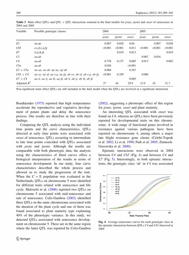
senescence curves per class are presented in Fig. 4.

The genotypic classes including ‘ab’ (fitted curves

with dashed line) had a faster onset and senescence

development than the classes in which ‘aa’ (fitted

curves with solid line) was present. The curve ‘ab ee’

showed a higher prate than ‘aa ee’ and the genotypes

in this class had in general a faster onset of

senescence and died earlier. The classes ‘aa fg’ and

‘ab fg’ were associated with late senescence devel-

opment and the prate and ipoint of these two classes

were the lowest. Genotypes in these two classes were

at almost half of the maximum senescence when the

observation period ended. Genotypes in the class ‘aa

fg’ showed the latest senescence development among

all the genotypic classes. Interestingly the class ‘ab

fg’ showed the earliest onset but this was followed by

a delayed senescence and the genotypes in this group

had the latest senescence.

Another epistatic interaction was observed in 2004

between C4 associated with onset and E7 related with

ipoint (Table 3). Figure 5 shows the average senes-

cence curves observed for the interaction C4 9 E7

with eight genotypic classes (‘aa ii’, ‘aa ij’, ‘aa ik’,

‘aa jk’, ‘ab ii’, ‘ab ij’, ‘ab ik’, ‘ab jk’) as shown in

Table 2. The classes including ‘ab’ (fitted curves with

dotted line) had in general, a faster senescence

development than classes in which ‘aa’ (solid line)

was present except for the class ‘aa ik’. In this class

earlier onset of the senescence process was observed

with a faster prate and ipoint while in the group ‘ab

ik’ a delayed onset with a slower prate is present.

Interestingly, big differences were also observed

between the classes ‘aa jk’ and ‘ab jk’. The class

‘aa jk’ showed the same trajectory than the class ‘aa

ii’ and both of them have late onset and ipoint making

the senescence process slower than in the other

classes. On the other hand, the class ‘ab jk’ showed

the earliest onset with a delayed senescence that

ended up simultaneously with the classes exhibiting

the slowest prate (‘aa ii’ and ‘aa jk’).

Discussion

The smoothed GLM procedure in our study allows

flexible modeling of different senescence curves in

the mapping population. Genotypes with early devel-

opment showed an s-shape senescence curve,

whereas genotypes with slow development exhibited

an exponential curve during the observation period.

In both cases the curve trajectories would eventually

reach the maximum of 7, which is the highest

senescence score. In the case of late genotypes, the

observation period was not long enough to complete

298 Euphytica (2012) 183:289–302

123

the senescence process. Four characteristics esti-

mated from the curves (onset, prate, mprate and

ipoint) allowed us to explain senescence in terms of

development. Whereas individual time points only

gave us an impression of the trait at selected different

moments during the growing season. In the first

case sensible biological interpretations could be

made and the results were compared with previous

studies describing the senescence process in the same

population evaluated in the Netherlands (Celis-

Gamboa 2002).

The weather and the general conditions of the

experiment had a clear effect on the performance of

the population in the 2 years of field experimentation

in Finland. Clearly the senescence period lasted

longer in 2005 and showed a slower progression

rate. This was probably due to the higher daily

air temperature observed that year. Marinus and

Table 2 Main effect QTLs and QTL 9 QTL interactions included in the full models for prate, ipoint and onset of senescence in

2004 and 2005

Variable Segregation typea Possible genotypic classesb 2004 2005

prate ipoint onset prate ipoint onset

E3 ‘‘nn 9 np’’ nn,np 0.86 0.032 0.003 0.856 0.006 0.011

Ch5 ‘‘ef 9 eg’’ ee,ef,e.g,fg \0.001 \0.001 0.007 \0.001 \0.001 \0.001

E7 ‘‘ij 9 ik’’ ii,ij,ik,jk 0.886 0.007 0.021 0.223 0.056 0.004

C1 ‘‘ab 9 aa’’ aa,ab 0.841 0.614 0.719 0.03 0.034 0.969

C4 ‘‘ab 9 aa’’ aa,ab 0.689 0.159 0.007 0.01 0.475 0.006

C5a ‘‘ab 9 aa’’ aa,ab 0.081 0.428 \0.001 0.763 0.076 0.154

E3 9 Ch5 ‘‘nn 9 np’’ 9 ‘‘ef 9 eg’’ nn ee, nn ef, nn e.g, nn fg, np ee,np ef, np e.g, np fg

0.838 0.117 0.293 0.829 0.486 0.563

E3 9 E7 ‘‘nn 9 np’’ 9 ‘‘ij 9 ik’’ nn ii, nn ij, nn ik, nn jk, np ii, npij, np ik, np jk

0.44 0.943 0.427 0.264 0.61 0.471

Ch5 9 E7 ‘‘ef 9 eg’’ 9 ‘‘ij 9 ik’’ ee ii, ee ij, ee ik, ee jk, ef ii, ef ij,ef ik, ef jk, e.g ii, e.g ij, e.g ik,e.g jk fg ii, fg ij, fg ik, fg jk

0.658 0.121 0.161 0.399 0.561 0.515

C1 9 C4 ‘‘ab 9 aa’’ 9 ‘‘ab 9 aa’’ aa aa, aa ab, ab aa, ab ab 0.93 0.178 0.139 0.566 0.398 0.925

C1 9 C5a ‘‘ab 9 aa’’ 9 ‘‘ab 9 aa’’ aa aa, aa ab, ab aa, ab ab 0.267 0.789 0.269 0.115 0.891 0.744

C4 9 C5a ‘‘ab 9 aa’’ 9 ‘‘ab 9 aa’’ aa aa, aa ab, ab aa, ab ab 0.302 0.701 0.264 0.426 0.075 0.325

E3 9 C1 ‘‘nn 9 np’’ 9 ‘‘ab 9 aa’’ nn aa, nn ab, np aa, np ab 0.392 0.33 0.62 0.396 0.75 0.906

E3 9 C4 ‘‘nn 9 np’’ 9 ‘‘ab 9 aa’’ nn aa, nn ab, np aa, np ab 0.373 0.701 0.895 0.909 0.784 0.574

E3 9 C5a ‘‘nn 9 np’’ 9 ‘‘ab 9 aa’’ nn aa, nn ab, np aa, np ab 0.019 0.657 0.037 0.5 0.366 0.922

Ch5 9 C1 ‘‘ef 9 eg’’ 9 ‘‘ab 9 aa’’ aa ee, aa ef, aa e.g, aa fg, ab ee,ab ef, ab e.g, ab fg

0.989 0.805 0.793 0.704 0.397 0.385

Ch5 9 C4 ‘‘ef 9 eg’’ 9 ‘‘ab 9 aa’’ aa ee, aa ef, aa e.g, aa fg, ab ee,ab ef, ab e.g, ab fg

0.043 0.039 0.47 0.022 0.736 0.977

Ch5 9 C5a ‘‘ef 9 eg’’ 9 ‘‘ab 9 aa’’ aa ee, aa ef, aa e.g, aa fg, ab ee,ab ef, ab e.g, ab fg

0.247 0.479 0.553 0.962 0.203 0.669

E7 9 C1 ‘‘ij 9 ik’’ 9 ‘‘ab 9 aa’’ aa ii, aa ij, aa ik, aa jk, ab ii, abij, ab ik, ab jk

0.414 0.566 0.959 0.904 0.57 0.948

E7 9 C4 ‘‘ij 9 ik’’ 9 ‘‘ab 9 aa’’ aa ii, aa ij, aa ik, aa jk, ab ii, abij, ab ik, ab jk

0.601 0.105 0.02 0.636 0.08 0.204

E7 9 C5a ‘‘ij 9 ik’’ 9 ‘‘ab 9 aa’’ aa ii, aa ij, aa ik, aa jk, ab ii, abij, ab ik, ab jk

0.294 0.475 0.88 0.691 0.265 0.708

Adjusted

R231.5 47.7 29.4 13.9 49.5 30.2

a Segregation type codes for a CP population according to MapQTL 6 (Van Ooijen 2009)b Genotype codes for a CP population, depending on the locus segregation type (Van Ooijen 2009) and the QTL 9 QTL interaction

Euphytica (2012) 183:289–302 299

123

Boadlaender (1975) reported that high temperatures

accelerate the reproductive and vegetative develop-

ment of potato plants and delay the senescence

process. Our results are therefore in line with their

findings.

Comparing the QTL analysis using the individual

time points and the curve characteristics, QTLs

detected at early time points were associated with

onset of senescence. QTLs occurring in intermediate

to late time points coincided with QTLs associated

with prate and ipoint. Although the results are

comparable with both phenotypic data, the analysis

using the characteristics of fitted curves offers a

biological interpretation of the results in terms of

senescence development. In our study, four curve

characteristics described the whole process and

allowed us to study the progression of the trait.

When the C 9 E population was evaluated in the

Netherlands, QTLs on chromosome 5 were identified

for different traits related with senescence and life

cycle. Malosetti et al. (2006) reported two QTLs on

chromosome 5 associated with mid-senescence and

rate of senescence. Celis-Gamboa (2002) identified

three QTLs on the same chromosome associated with

the duration of the plant cycle and one of them was

found associated to plant maturity type explaining

40% of the phenotypic variance. In this study, we

detected QTLs associated with senescence develop-

ment on chromosome 5. These are in the same region

where the latter QTL was reported by Celis-Gamboa

(2002), suggesting a pleiotropic effect of this region

for prate, ipoint, onset and plant maturity.

An interesting QTL associated with onset was

found on C4, whereas no QTLs have been previously

reported for developmental traits on this chromo-

some. A wide range of functional genes involved in

resistance against various pathogens have been

reported on chromosome 4, among others a major

late blight resistance gene cluster (Celebi-Toprak

et al. 2002; Li et al. 1998; Park et al. 2005; Zimnoch-

Guzowska et al. 2000).

Epistatic interactions were observed in 2004

between C4 and Ch5 (Fig. 4) and between C4 and

E7 (Fig. 5). Interestingly, in both epistatic interac-

tions, the genotypic class ‘ab’ in C4 was associated

Table 3 Main effect QTLs and QTL 9 QTL interactions retained in the final models for prate, ipoint and onset of senescence in

2004 and 2005

Variable Possible genotypic classes 2004 2005

prate ipoint onset prate ipoint onset

E3 nn,np 0.887 0.028 0.04 0.007 0.028

Ch5 ee,ef,e.g,fg \0.001 \0.001 0.011 \0.001 \0.001 \0.001

E7 ii,ij,ik,jk 0.019 0.013 0.019

C1 aa,ab 0.067 0.016

C4 aa,ab 0.738 0.157 0.005 0.013 0.002

C5a aa,ab 0.026 \0.001

E3 9 C5a nn aa, nn ab, np aa, np ab 0.066 0.267

Ch5 9 C4 aa ee, aa ef, aa e.g, aa fg, ab ee, ab ef, ab e.g, ab fg \0.001 0.109 0.086

E7 9 C4 aa ii, aa ij, aa ik, aa jk, ab ii, ab ij, ab ik, ab jk 0.005

Adjusted R2 37 44 29.9 13.9 43 31.7

Non-significant main effect QTLs are still included in the final model when the QTLs are involved in a significant interaction

Fig. 4 Average senescence curves for each genotypic class in

the epistatic interaction between QTLs C4 and Ch5 observed in

2004

300 Euphytica (2012) 183:289–302

123

with early development of the senescence process. In

the interaction C4 9 Ch5, the genotypic classes ‘ab

ee’ and ‘ab ef’ associated with early senescence

showed delayed onset but fast prate and ipoint

whereas the class ‘ab fg’’ showed early onset but a

senescence period lasting longer. In 2005 no epistatic

interactions were observed but main effects of C1 and

pleiotropic effects of E3 and C4 on ipoint/onset and

prate/onset, respectively.

In summary, by modeling haulm senescence in the

C 9 E potato population using a smoothed GLM

procedure, we were able to characterize the curve in

terms of developmental traits and to identify QTLs

associated with the senescence process. Pleiotropic

effects and epistatic interactions between QTLs were

detected when two-way interactions were studied.

Delayed senescence was associated with particular

genotypic classes (C4 9 Ch5: ‘ab fg’ and C4 9 E7:

‘aa ii’ ‘aa jk’) and some classes showing early onset

turned to have delayed senescence development

(C4 9 Ch5: ‘ab fg’ and C4 9 E7: ‘ab jk’).

Different regulatory genes have been reported for

onset and progression rate of senescence in Arabid-

opsis thaliana (Gepstein et al. 2003) and it will be

interesting to compare the genes involved in the same

process in different crops. The complexity of

QTL 9 E and QTL 9 QTL 9 E as well as the

performance of genotypes under different environ-

ments will be considered in a further study providing

insights for the better understanding of adaptation and

developmental processes in potato.

Acknowledgments We thank Prof. Paul Struik (Centre for

Crop Systems Analysis, Wageningen University) for the

discussion on the use of beta-thermal time in this study. Part

of this project was (co)financed by the Centre for BioSystems

Genomics (CBSG) which is part of the Netherlands Genomics

Initiative/Netherlands Organisation for Scientific Research.

Open Access This article is distributed under the terms of the

Creative Commons Attribution Noncommercial License which

permits any noncommercial use, distribution, and reproduction

in any medium, provided the original author(s) and source are

credited.

References

Allaby M (1998) A dictionary of plant sciences. Encyclope-

dia.com. http://www.encyclopedia.com. Accessed 30

November 2009

Benoit RG, Grant WJ, Devine OJ (1986) Potato top growth as

influenced by day–night temperature differences. Agron J

78:264–269

Celebi-Toprak F, Slack SA, Jahn MM (2002) A new gene,

Nytbr, for hypersensitivity to Potato virus Y from Solanumtuberosum maps to chromosome IV. Theor Appl Genet

104:669–674

Celis-Gamboa BC (2002) The life cycle of the potato (Solanumtuberosum L.): from crop physiology to genetics. PhD

Thesis. Wageningen University, Wageningen

Celis-Gamboa C, Struik PC, Jacobsen E, Visser RGF (2003)

Temporal dynamics of tuber formation and related

processes in a crossing population of potato (Solanumtuberosum). Ann Appl Biol 143:175–186

Eilers PHC, Marx BD (1996) Flexible smoothing with

B-splines and penalties. Stat Sci 11(2):89–121

Ewing EE, Struik PC (1992) Tuber formation in potato:

induction, initiation and growth. Hortic Rev 14:89–198

Gao LZ, Jin ZQ, Huang Y, Zhang LZ (1992) Rice clock

model—a computer simulation model of rice develop-

ment. Agric For Meteorol 60:1–16

Gepstein S, Sabehi G, Carp M-J, Hajouj T, Nesher MFO, Yariv

I, Dor C, Bassani M (2003) Large-scale identification of

leaf senescence-associated genes. Plant J 36:629–642

Hanneman RE, Peloquin SJ (1967) Crossability of 24 chro-

mosome potato hybrids with 48 chromosome cultivars.

Eur Potato J 10:62–73

Haun JR (1975) Potato growth-environment relationship. Agric

Meteorol 15:325–332

Hawkes JG (1990) The potato: evolution, biodiversity and

genetic resources. Belhaven press, London, p 259

Hodges T (1991) Temperature and water stress effects on

phenology. In: Hodges T (ed) Predicting crop phenology.

CRC Press, Boca Raton, pp 7–13

Jacobsen E (1980) Increase of diplandroid formation and seed

set in 4x 9 2x crosses in potatoes by genetical manipu-

lation of dihaploids and some theoretical consequences.

Z Pflanzenzuecht 85:110–121

Johnson IR, Thornley JHM (1985) Temperature dependence of

plant and crop processes. Ann Bot 55:l–24

Khan MS, Struik PC, van der Putten PEL, van Eck HJ, van

Eeuwijk FA, Yin X (2011) Analyzing genetic variation in

Fig. 5 Average senescence curves for each genotypic class in

the epistatic interaction between QTLs C4 and E7 observed in

2004

Euphytica (2012) 183:289–302 301

123

potato (Solanum tuberosum) canopy dynamics using

standard cultivars and a segregating population. (Under

review)

Li X, van Eck HJ, Rouppe van der Voort JNAM, Huigen DJ,

Stam P, Jacobsen E (1998) Autotetraploids and genetic

mapping using common AFLP markers: the R2 allele

conferring resistance to Phytophthora infestans mapped

on potato chromosome 4. Theor Appl Genet 96:

1121–1128

Ma C-X, Casella G, Wu R (2002) Functional mapping of

quantitative trait loci underlying the character process: a

theoretical framework. Genetics 161:1751–1762

Malosetti M, Visser RGF, Celis-Gamboa C, van Eeuwijk FA

(2006) QTL methodology for response curves on the basis

of non-linear mixed models, with an illustration to

senescence in potato. Theor Appl Genet 113:288–300

Marinus J, Boadlaender KBA (1975) Response of some potato

varieties to temperature. Potato Res 18:189–204

Nelder JA, Wedderburn RWM (1972) Generalized linear

models. J Royal Stat Soc, Series A 135:370–384

Park TH, Gros A, Sikkema A, Vleeshouwers VGAA, Muskens

M, Allefs S, Jacobsen E, Visser RGF, van der Vossen

EAG (2005) The late blight resistance locus Rpi-blb3from Solanum bulbocastanum belongs to a major late

blight R gene cluster on chromosome 4 of potato. Mol

Plant Microbe Interact 18:722–729

Payne RW, Murray DA, Harding SA, Baird DB, Soutar DM

(2010) An introduction to GenStat for Windows, 13th edn.

VSN International, Hemel Hempstead, UK

Reymond M, Muller B, Leonardi A, Charcosset A, Tardieu F

(2003) Combining quantitative trait loci analysis and an

ecophysiological model to analyze the genetic variability

of the responses of maize leaf growth to temperature and

water deficit. Plant Physiol 131:664–675

Schnute J (1981) A versatile growth model with statistically

stable parameters. Can J Fish Aquat Sci 38:1128–1140

Struik PC, Ewing EE (1995) Crop physiology of potato:

responses to photoperiod and temperature relevant to crop

modeling. In: Haverkort AJ, MacKerron DKL (eds)

Potato ecology and modeling of crops under conditions

limiting growth. Kluwer Acad Publ, Boston, pp 19–40

van Ooijen JW (2006) JoinMap 4, Software for the calculation

of genetic linkage maps in experimental populations.

Kyazma B.V, Wageningen, the Netherlands

van Ooijen JW (2009) MapQTL 6, Software for the mapping of

quantitative trait loci in experimental populations of dip-

loid species. Kyazma B.V, Wageningen, the Netherlands

Werij JS, Kloosterman B, Celis-Gamboa C, de Vos CHR,

America T, Visser RGF, Bachem C (2007) Unravelling

enzymatic discoloration in potato through a combined

approach of candidate genes, QTL, and expression anal-

ysis. Theor Appl Genet 115:245–252

Wu RL, Lin M (2006) Functional mapping—how to map and

study the genetic architecture of dynamic complex traits.

Nat Rev Gene 7:229–237

Wu RL, Ma CX, Zhao W, Casella G (2003) Functional map-

ping of quantitative trait loci underlying growth rates: a

parametric model. Physiol Genomics 14:241–249

Yin X, Kropff MJ, McLaren G, Visperas RM (1995) A non-

linear model for crop development as a function of tem-

perature. Agric For Meteorol 77:1–16

Zaban A, Vetelainen M, Celis-Gamboa C, van Berloo R,

Haggman H, Visser RGF (2006) Physiological and

genetic aspects of a diploid potato population in the

Netherlands and Northern Finland. Maataloustieteen Pai-

vat 2006:1–7

Zimnoch-Guzowska E, Marczewski E, Lebecka R, Flis B,

Schafer-Pregl R, Salamini F, Gebhardt C (2000) QTL

analysis of new sources of resistance to Erwinia caroto-vora ssp. atroseptica in potato done by AFLP, RFLP, and

resistance-gene-like markers. Crop Sci 40:1156–1167

302 Euphytica (2012) 183:289–302

123