F Fermi National Accelerator Laboratory

FERMILAB-Pub-96/222-A

Dynamical � Models of Structure Formation

Kimberly Coble, Scott Dodelson and Joshua A. Frieman

Fermi National Accelerator LaboratoryP.O. Box 500, Batavia, Illinois 60510

August 1996

Submitted to Physical Review D

Operated by Universities Research Association Inc. under Contract No. DE-AC02-76CHO3000 with the United States Department of Energy

Disclaimer

This report was prepared as an account of work sponsored by an agency of the United States

Government. Neither the United States Government nor any agency thereof, nor any of

their employees, makes any warranty, expressed or implied, or assumes any legal liability or

responsibility for the accuracy, completeness, or usefulness of any information, apparatus,

product, or process disclosed, or represents that its use would not infringe privately owned

rights. Reference herein to any speci�c commercial product, process, or service by trade

name, trademark, manufacturer, or otherwise, does not necessarily constitute or imply its

endorsement, recommendation, or favoring by the United States Government or any agency

thereof. The views and opinions of authors expressed herein do not necessarily state or re ect

those of the United States Government or any agency thereof.

Distribution

Approved for public release; further dissemination unlimited.

FERMILAB{Pub{96/222-A

August 1996

submitted to Physical Review D

Dynamical � Models of Structure Formation

Kimberly Coble1;2

Scott Dodelson2

Joshua A. Frieman1;2

1Department of Astronomy and Astrophysics

The University of Chicago, Chicago, IL 60637

2NASA/Fermilab Astrophysics Center

Fermi National Accelerator Laboratory, Batavia, IL 60510-0500

ABSTRACT

Models of structure formation with a cosmological constant � provide a good �t to the

observed power spectrum of galaxy clustering. However, they su�er from several problems.

Theoretically, it is di�cult to understand why the cosmological constant is so small in Planck

units. Observationally, while the power spectra of cold dark matter plus � models have ap-

proximately the right shape, the COBE-normalized amplitude for a scale invariant spectrum

is too high, requiring galaxies to be anti-biased relative to the mass distribution. Attempts

to address the �rst problem have led to models in which a dynamical �eld supplies the vac-

uum energy, which is thereby determined by fundamental physics scales. We explore the

implications of such dynamical � models for the formation of large-scale structure. We �nd

that there are dynamical models for which the amplitude of the COBE-normalized spectrum

matches the observations. We also calculate the cosmic microwave background anisotropies

in these models and show that the angular power spectra are distinguishable from those of

standard cosmological constant models.

1 Introduction

The cosmological constant has had a long and tortured history since Einstein �rst intro-

duced it in 1917 in order to obtain static cosmological solutions [1]. Under observational

duress, it has been periodically invoked by cosmologists and then quickly forgotten when

the particular crisis passed. Historical examples include the �rst `age crisis' arising from

Hubble's large value for the expansion rate (1929), the apparent clustering of QSO's at a

speci�c redshift (1967), and early cosmological tests which indicated a negative deceleration

parameter (1974).

Recently, a cosmological model with substantial vacuum energy|a relic cosmological

constant �|has again come into vogue for several reasons[2]. First, dynamical estimates of

the mass density on the scales of galaxy clusters, the largest gravitationally bound systems,

suggest that m = 0:2 � 0:1 for the matter (m) which clusters gravitationally (where is

the present ratio of the mean mass density of the universe to the critical Einstein-de Sitter

density, = 8�G�=3H2) [3]. However, if a su�ciently long epoch of in ation took place

during the early universe, the present spatial curvature should be negligibly small, tot = 1.

A cosmological constant, with e�ective density parameter � � �=3H20 = 1 � m, is one

way to resolve the discrepancy between m and tot.

The second motivation for the revival of the cosmological constant is the `age crisis'

for spatially at m = 1 models. Current estimates of the Hubble expansion parame-

ter from a variety of methods appear to be converging to H0 ' 70 � 10 km/sec/Mpc,

while estimates of the age of the universe from globular clusters are holding at tgc '13 � 15 Gyr or more. Thus, observations imply a value for the the `expansion age' H0t0 =

(H0=70 km=sec=Mpc)(t0=14 Gyr) ' 1:0 � 0:2. This is higher than that for the standard

Einstein-de Sitter model with m = 1, for which H0t0 = 2=3. On the other hand, for models

with a cosmological constant, H0t0 can be larger. For example, for � = 0:6 = 1 � m,

H0t0 = 0:89.

Third, cold dark matter (CDM) models for large-scale structure formation which include

a cosmological constant (hereafter, �CDM) provide a better �t to the shape of the observed

power spectrum of galaxy clustering than does the `standard' m = 1 CDM model [4].

Figure 1 shows the inferred galaxy power spectrum today (based on a recent compilation

[5]), compared with the matter power spectra predicted by standard CDM and a �CDM

model with � = 0:6. In both cases, the Hubble parameter has been �xed to h � H0=(100

km/sec/Mpc) = 0:7 and the baryon density to B = 0:0255, in the center of the range allowed

1

by primordial nucleosynthesis. Linear perturbation theory has been used to calculate the

model power spectra, P (k), de�ned by h�(k)��(k0)i = (2�)3P (k)�D(k � k0), where �(k) is

the Fourier transform of the spatial matter density uctuation �eld and �D is the Dirac delta

function. Here and throughout, we have taken the primordial power spectrum to be exactly

scale-invariant, Pprimordial(k) / kn with n = 1. Standard CDM clearly gives a poor �t to the

shape of the observed spectrum [6], while the �CDM model gives a good �t to the shape

of the observed spectrum. The amplitudes of the model spectra in Fig. 1 have been �xed

at large scales by observations of cosmic microwave background (CMB) anisotropies by the

COBE satellite [7, 8].

Despite these successes, cosmological constant models face several di�culties of their

own. On aesthetic grounds, it is di�cult to understand why the vacuum energy density of

the universe, �� � �=8�G, should be of order (10�3eV)4, as it must be to have a cosmological

impact (� � 1). On dimensional grounds, one would expect it to be many orders of

magnitude larger { of order m4Planck or perhaps m

4SUSY . Since this is not the case, we might

plausibly assume that some physical mechanism sets the ultimate vacuum energy to zero.

Why then is it not zero today?

The cosmological constant is also increasingly observationally challenged. Preliminary

results from on-going searches[9] for distant Type Ia supernovae indicate that � < 0:47 (at

95% con�dence) for spatially at � models. Furthermore, in � models a larger fraction of

distant QSOs would be gravitationally lensed than in a � = 0 universe; surveys for lensed

QSOs have been used to infer the bound � <� 0:7 [10].

In this paper, we focus on a third problem of cosmological constant models|the ampli-

tude of the power spectrum of galaxy clustering. The shape of the �CDM power spectrum

in Figure 1 matches the galaxy power spectrum; however the amplitude is too high. Indeed

a number of analyses have found that this problem persists on all scales:

� On the largest scales (k < 0:1h Mpc�1), linear theory should be adequate, and Figure

1 suggests that the amplitude is too high by at least a factor of two.

� On intermediate scales, we can quantify the amplitude through the dispersion of the

density �eld smoothed over top-hat spheres of radius R = 8h�1 Mpc, denoted �8,

where �2(R) = 4�R1

0 k2P (k)W 2(kR)dk, and W (kR) is the Fourier-transform of the

spatial top-hat window function of radius R. In the �CDM model of Figure 1, COBE

normalization yields �8 ' 1:3 [8], while galaxy surveys generally indicate �8;gal ' 1

for optically selected galaxies and � 0:8 for galaxies selected by infrared ux. This

2

high COBE normalization also marginally con icts with the abundance of rich galaxy

clusters [11]. Using the observed cluster X-ray temperature distribution function and

modelling cluster formation using Press-Schechter theory, for this �CDM model the

cluster abundance implies �8 ' 1:0+:35�:26 [12], where the errors are approximate 95%

con�dence limits.

� N-body simulations indicate that the power spectrum amplitude is higher by a factor

of two to three than that found in galaxy surveys at small scales, k >� 0:4h Mpc�1 [13].

Thus, the cosmological constant model would require galaxies to be substantially anti-

biased with respect to the mass distribution, �gal < ��. Models of galaxy formation,

however, suggest that the bias parameter, b � �gal=��, is greater than unity [14, 15].

Motivated by these di�culties, we consider models in which the energy density resides in a

dynamical scalar �eld rather than in a pure vacuum state. These dynamical � models [16, 17]

were proposed in response to the aesthetic di�culties of cosmological constant models. They

were also found [16] to partially alleviate their observational problems as well; for example,

the statistics of gravitationally lensed QSOs yields a less restrictive upper bound on H0t0

in these models[18]. We emphasize here that they may also solve the galaxy clustering

amplitude problem.

To get a preview of this conclusion, Fig. 1 also shows the COBE normalized power spec-

trum for a dynamical � model with present scalar �eld density parameter � = 0:6 (see x3for a discussion of these models). While the shape of the spectrum is identical to that of the

�CDM model with � = 0:6, the scalar �eld model has a lower amplitude, and thus provides

a better �t to the galaxy clustering data. In x2, we explain these features of the power spec-trum for the standard �CDM model and for generic dynamical � models. The remaining

sections investigate in detail a speci�c class of models as a worked example. Section 3 re-

views the scalar �eld model, based on ultra-light pseudo-Nambu-Goldstone bosons (PNGBs)

[16]. To explore the parameter space of this model, we have adapted a code which solves

the linearized Einstein-Boltzmann equations for perturbations to a Friedmann-Robertson-

Walker (FRW) background. The appendices contain details of these modi�cations. Section

4 discusses the qualitative features of cosmic evolution in the PNGB models and presents

results of our calculation for the amplitude of the power spectrum in this model. In x5 we

present the cosmic microwave background (CMB) power spectrum for a particular set of

model parameters, followed by the conclusion.

3

2 The Power Spectrum

2.1 The Shape of P (k)

Figure 1 suggests that standard CDM could be improved by simply shifting the turnover in

the power spectrum to larger scales (smaller wavenumber k). This is a plausible �x, for the

location of the turnover corresponds to the scale that entered the Hubble radius when the

universe became matter-dominated. On scales smaller than this, the uctuation amplitude is

suppressed compared to that on larger scales, because matter perturbations inside the Hubble

radius cannot grow in a radiation-dominated universe. This scale is determined by the ratio

of matter to radiation energy density at early times. To \�x" CDM, one must decrease the

ratio ��m=��r in the universe today below that predicted by the standard Einstein-de Sitter

model. The matter and radiation densities scale as ��m = ��m;0a�3 and ��r = ��r;0a�4, where the

cosmic scale factor a is normalized to unity today (a0 = 1) and the subscript 0 denotes the

present. Thus the epoch of matter-radiation equality is determined by the present energy

densities of matter and radiation:

aEQ =��r;0��m;0

=4:3� 10�5

mh2: (1)

Decreasing the matter to radiation density ratio shifts the epoch of matter-radiation equality

closer to the present, thereby moving the turnover in the power spectrum to larger scales.

Indeed, this shift is precisely what is done in several currently popular models of structure

formation. Examples include i) models with a lower Hubble constant than indicated by

observations[19], ii) models with extra relativistic degrees of freedom[20], and iii) models

with a cosmological constant[4]. Since ��m / mh2, a lower Hubble constant decreases the

ratio of matter to radiation density today. Adding more relativistic degrees of freedom adds

to the radiation content, decreasing the ratio of matter to radiation. Finally, in spatially

at � models, m � 1�� is reduced from its standard CDM value (m = 1), achieving a

similar e�ect.

Thus the main bene�t of � models for the shape of the power spectrum is that m is

smaller than in the standard CDM model. For the purpose of the power spectrum shape,

the value of the vacuum energy density at early times is irrelevant, as long as it is negligible

compared to the matter and radiation densities at matter-radiation equality. While the time

dependence of the vacuum energy density is di�erent for various dynamical � models, all

such models yield the same power spectrum shape for a �xed value of the present vacuum

energy density. We emphasize this point in Fig. 2, which shows the energy densities of

4

matter, radiation, �, and a speci�c dynamical � model (scalar �eld �), as a function of scale

factor a. With � and � = 0:6 today, the standard and dynamical � models have the same

shape for P (k) (shown in Fig. 1), since they have identical values of aEQ. As we will see

below, however, the amplitudes of the power spectra in these models di�er substantially.

2.2 The Amplitude of P (k)

Compared to standard CDM, three new physical e�ects [21] conspire to change the ampli-

tude of the matter power spectrum in COBE-normalized � models: i) the suppression of

growth of perturbations when the universe becomes �-dominated, ii) the reduced gravita-

tional potential, and iii) the integrated Sachs-Wolfe (ISW) e�ect. We review these e�ects in

turn.

The equations governing large scale perturbations in a at universe with matter and

vacuum energy are

�� +Ha _� � 3

2a2H2m� = 0 (2)

H2 =H2

0

a3

"m + �

����;0

a3#

(3)

Here overdots denote derivatives with respect to conformal time � , where � � Rdt=a(t),

�� is the vacuum energy density, not necessarily equal to its present value ��;0, the density

uctuation amplitude �(x; � ) � (�m(x; � )� ��m(� ))=��m(� ), and H is the Hubble expansion

rate [we use units in which �h = c = 1].

Equation 2 essentially describes the behavior of a damped harmonic oscillator. When the

energy density of the universe becomes dominated by a � or dynamical �, i.e., the second

term on the the RHS in equation 3 becomes important, the damping becomes more severe.

When this happens, the growth of perturbations is suppressed. As a function of m, this

suppression can be described by the scaling,

�0=�(z=100) / pm; (4)

where �0 is the perturbation amplitude today, and �(z=100) is the amplitude at the epoch

z � (1=a)� 1 = 100, chosen as an arbitrary early epoch before the vacuum energy becomes

dynamically important. In �CDMmodels, p ' 0:2. For dynamical � models, the suppression

exponent depends on the details of the speci�c model, but it is generally greater than that in

�CDM models, because the dynamical � dominates earlier in the history of the universe for

�xed ��;0. For the model shown in Fig. 1, p ' 0:56. For open CDM models (with � = 0),

the scaling is also p ' 0:56.

5

As a result of this suppression, one might expect the amplitude of the power spectrum in

�CDM and dynamical � models to be smaller than that in standard CDM. However, from

the Poisson equation

r2� =3

2a2H2m� ; (5)

we have � / m�, where � is the gravitational potential associated with large-scale density

uctuations. Since the CMB anisotropy at large angle is a well-de�ned function of the

potential[22], COBE normalization corresponds to �xing the potential, i.e., to �xing m�.

For COBE-normalized models, the growth suppression and Poisson's equation combine to

yield the scale-independent relation � / p�1m . Thus the power spectrum P (k) / �2 / �1:6m

in �CDMmodels. A larger cosmological constant implies a smaller m, which in turn implies

a larger amplitude for the power spectrum. In dynamical � models, p is not �xed at 0:2,

so the amplitude of the power spectrum can be smaller than in standard � models. For the

model of Fig. 1, with p = 0:56, P (k) / �0:9m .

The integrated Sachs-Wolfe e�ect (ISW), which is due to time evolution of the potential,

also a�ects the amplitude of the power spectrum. The changing potential at late times in

� models increases the anisotropy on the large angular scales probed by COBE. Thus, for

�xed COBE normalization, the amplitude of the power spectrum decreases, changing the

dependence of the power spectrum on m to P / �1:4m in the �CDM model. In dynamical

� models, where the potential typically changes more than in standard � models, the ISW

e�ect tends to be larger and is not a power law function of m. Hence the power spectrum

amplitude in dynamical models is even less enhanced than in �CDM models, and can even

be reduced compared to standard CDM.

3 Ultra-light Scalar Fields

A number of models with a dynamical � have been discussed in the literature [17]. We will

focus on a particular class of models motivated by the physics of pseudo-Nambu-Goldstone

bosons (hereafter PNGBs) [16, 23].

It is conventional to assume that the fundamental vacuum energy of the universe is zero,

owing to some as yet not understood mechanism, and that this mechanism `commutes' with

other dynamical e�ects that lead to sources of energy density. This is required so that, e.g.,

at earlier epochs there can temporarily exist non-zero vacuum energy which allows in ation

to take place. With these assumptions, the e�ective vacuum energy at any epoch will be

dominated by the heaviest �elds which have not yet relaxed to their vacuum state. At late

6

times, these �elds must be very light.

Vacuum energy is most simply stored in the potential energy V (�) � M4 of a scalar

�eld, where M sets the characteristic height of the potential, and we set V (�m) = 0 at the

minimum of the potential by the assumptions above. In order to generate a non-zero � at

the present epoch, � must initially be displaced from the minimum (�i 6= �m as an initial

condition), and its kinetic energy must be small compared to its potential energy. This

implies that the motion of the �eld is still overdamped, m� �qjV 00(�i)j <� 3H0 = 5�10�33h

eV. In addition, for � � 1, the potential energy density should be of order the critical

density, M4 � 3H20M

2P l=8�, or M ' 3 � 10�3h1=2 eV. Thus, the characteristic height and

curvature of the potential are strongly constrained for a classical model of the cosmological

constant.

This argument raises an apparent di�culty for such a model: why is the mass scale m�

thirty orders of magnitude smaller than M? In quantum �eld theory, ultra-low-mass scalars

are not generically natural: radiative corrections generate large mass renormalizations at

each order of perturbation theory. To incorporate ultra-light scalars into particle physics,

their small masses should be at least `technically' natural, that is, protected by symmetries,

such that when the small masses are set to zero, they cannot be generated in any order of

perturbation theory, owing to the restrictive symmetry.

From the viewpoint of quantum �eld theory, PNGBs are the simplest way to have natu-

rally ultra{low mass, spin{0 particles. PNGB models are characterized by two mass scales,

a spontaneous symmetry breaking scale f (at which the e�ective Lagrangian still retains the

symmetry) and an explicit breaking scale � (at which the e�ective Lagrangian contains the

explicit symmetry breaking term). In terms of the mass scales introduced above, generally

M � � and the PNGB mass m� � �2=f . Thus, the two dynamical conditions on m� and M

above essentially �x these two mass scales to be � �M � 10�3 eV, interestingly close to the

neutrino mass scale for the MSW solution to the solar neutrino problem, and f �MP l ' 1019

GeV, the Planck scale. Since these scales have a plausible origin in particle physics models,

we may have an explanation for the `coincidence' that the vacuum energy is dynamically

important at the present epoch. Moreover, the small mass m� is technically natural.

An example of this phenomenon is the `schizon' model [23], based on a ZN -invariant

low-energy e�ective chiral Lagrangian for N fermions, e.g., neutrinos, with mass of order M ,

in which the small PNGB mass, m� ' M2=f , is protected by fermionic chiral symmetries.

The potential for the light scalar �eld � is of the form

V (�) = M4[cos(�=f) + 1] : (6)

7

Since � is extremely light, we assume that it is the only classical �eld which has not yet

reached its vacuum expectation value. The constant term in the PNGB potential has been

chosen to ensure that the vacuum energy vanishes at the minimum of the � potential, in

accord with our assumption that the fundamental vacuum energy is zero.

4 Cosmic Evolution and Large-scale Power Spectrum

in PNGB Models

To study the cosmic evolution of these models, we focus on the spatially homogeneous,

zero-momentum mode of the �eld, �(0)(� ) = h�(x; � )i, where the brackets denote spatial

averaging. We are assuming that the spatial uctuation amplitude ��(x; � ) is small compared

to �(0), as would be expected after in ation if the post-in ation reheat temperature TRH <

f �Mpl. The scalar equation of motion is given in Appendix A.

The cosmic evolution of � is determined by the ratio of its mass, m� � M2=f , to the

instantaneous expansion rate, H(� ). For m� <� 3H, the �eld evolution is overdamped by

the expansion, and the �eld is e�ectively frozen to its initial value �i. Since � is initially

laid down in the early universe (at a temperature T � f � M) when its potential was

dynamically irrelevant, its initial value in a given Hubble volume will generally be displaced

from its vacuum expectation value �m = �f (vacuum misalignment). Thus, at early times,

the �eld acts as an e�ective cosmological constant, with vacuum energy density and pressure

�� ' �p� � M4. At late times, m� � 3H(� ), the �eld undergoes damped oscillations

about the potential minimum; at su�ciently late times, these oscillations are approximately

harmonic, and the stress-energy tensor of � averaged over an oscillation period is that of

non-relativistic matter, with energy density �� � a�3 and pressure p� ' 0.

Let �x denote the epoch when the �eld becomes dynamical, m� = 3H(�x), with corre-

sponding redshift 1 + zx = 1=a(�x)) = (M2=3H0f)2=3. For comparison, the universe makes

the transition from radiation- to matter-domination at zeq ' 2:3 � 104mh2, much earlier

than when the �eld becomes dynamical. The f �M parameter space is shown in Fig. 3.

In the far right portion of the �gure, the �eld becomes dynamical before the present epoch

and currently redshifts as non-relativistic matter; on the far left, � is still frozen and acts

as an ordinary cosmological constant. In the dynamical region, the present density param-

eter for the scalar �eld is approximately � � 24�(f=MP l)2, independent of M [24]. The

quasi-horizontal lines show contours of constant �, assuming a typical initial �eld value

�i=f = 1:6 (we will use this value of �i=f for all the plots below; the quoted limits and

8

results depend slightly on it). The limit � < 1 corresponds approximately to f < 3:5�1018

GeV. In the frozen region, on the other hand, � is determined byM4, independent of f , and

the contours of constant � are nearly vertical. In this region, the bound � < 1 corresponds

roughly to M < 0:003 eV.

Figure 4 shows contours of constant H0t0 in the same parameter space. As expected,

models with large H0t0 are concentrated toward the left hand portion of the �gure; as one

moves to the right, H0t0 asymptotically approaches the Einstein-de Sitter value 2=3, since

the scalar �eld currently redshifts as non-relativistic matter and we have assumed a spatially

at universe. Consequently, the `interesting' region of parameter space is the area near the

`corner' in Figs. 3 and 4, in which the �eld becomes dynamical at recent epochs, zx � 0� 3.

This has new consequences, compared to � models, for the classical cosmological tests, the

expansion age H0t0, and large-scale structure. In this region, the mass of the PNGB �eld is

miniscule, m� � 3H0 � 4 � 10�33 eV, and (by construction) its Compton wavelength is of

order the current Hubble radius, �� = m�1� = H�1

0 =3 � 1000h�1 Mpc.

Figure 5 shows contours of the amplitude of galaxy clustering in the f �M parameter

space. The amplitude shown is the quantity

limk!0

"(P (k)=k)�(P (k)=k)�

#; (7)

i.e., the amplitude on large scales relative to that for a �CDM model with the same e�ective

density as the PNGB model, � = �. This amplitude ratio goes to unity in the left-hand

portion of the �gure since that region corresponds to a �CDMmodel. However the amplitude

ratio can be substantially below one in the dynamical region on the right. The cross marks

the speci�c choice M = 0:005 eV, f = 1:885 � 1018 GeV, with initial �eld value �i=f = 1:6,

yielding � = 0:6, which corresponds to the parameters used for the dynamical � curves

in Figs. 1 and 2. For this case, the X-ray cluster abundance yields �cl8 ' 0:9+:3�:2, in good

agreement with the COBE normalization �COBE8 ' 0:8 for this model. Figure 6 shows how

density perturbations grow in the di�erent models. From Eqn.(4) and the text following,

the dynamical � model has a higher amplitude at early times than a �CDM model with

the same amplitude today. As a consequence, there should be no problem accounting for

high-redshift objects such as QSOs and Lyman-alpha clouds in this model.

Note that the factor �(z)=�0, relative to its value in the standard CDM model, approaches

�pm at z � 1, where p is the scaling exponent discussed in x2. As a result, the non-linear

behavior of the dynamical � model follows that of an open model with the same value of

m. We estimate the non-linear behavior by using the �tting formula of Ref. [25], following

9

the original treatment [26] of Hamilton et al. Figure 7 shows these non-linear spectra. On

scales k � 1hMpc�1, the amplitude of the power spectrum is indeed a factor of two smaller

in the dynamical � model than in the corresponding �CDM model.

We note by comparing Figs. 4 and 5 that the region of parameter space in which the

amplitude (anti-bias) problem is solved, i.e., in which the amplitude ratio is approximately

in the range 0:3 � 0:5, is the one in which the age of the universe is only slightly greater

than in the Einstein-de Sitter m = 1 case. For our speci�c model above, H0t0 = 0:73. For

the corresponding �CDM model with the same value of m, H0t0 = 0:89, more comfortably

within the observational limits. This is a general feature of the dynamical models considered

here: for �xed m, the standard � model gives an upper bound onH0t0. Thus, the amplitude

problem in this model is resolved partially at the expense of the age problem. On the other

hand, the q0 constraints from SNe and gravitational lensing translate into weaker upper

bounds on H0t0 for the dynamical as opposed to the standard � models. Although we

have not thorougly examined all models, it is clear that one could explore the PNGB model

parameter space to obtain a more balanced compromise between the age problem and the

anti-bias problem. For example, for f ' 2:5� 1018 GeV and M ' 0:0035 eV, the amplitude

ratio is about 0.5, and one has � ' 0:75 and H0t0 ' 0:9. In this case, with h = 0:7, the

power spectrum shape is reasonable (mh ' 0:15) and the age of the universe is t ' 12:6

Gyr.

Comparing Figs. 3 and 5, and focusing on the dynamical region near the `corner' of the

parameter space, we see that the power spectrum shape and amplitude constraints �x the

free parameters of the model. That is, as noted in x2, the shape of the spectrum is �xed by

requiring � ' 0:6, which determines the scale f . Near the corner, �xing the amplitude then

determines the other mass scaleM . While these �gures correspond to a speci�c choice of the

initial �eld value �i=f , the scalar �eld evolution is universal in the sense that a shift in the

mass scale f , accompanied by an appropriate rescaling of �i, leads to essentially identical

evolution. Consequently, compared to �CDM models, these dynamical models have only

one additional free parameter, the mass M , to solve the amplitude (anti-bias) problem.

5 CMB Anisotropy

The angular power spectra of the cosmic microwave background (CMB) anisotropy for dy-

namical � models are distinguishable from those of standard CDM and �CDM models.

CMB angular power is usually expressed in terms of the angular multipoles Cl. If the sky

10

temperature is expanded in terms of spherical harmonics as T (�; �) = �lmalmYlm(�; �), then

Cl = hjalmj2i, where large l corresponds to small angular scales. The angular power spec-

tra for standard CDM (m = 1), �CDM, and dynamical � models (the latter two with

m = 0:4) are shown in Figures 8 and 9 for h = 0:7, B = 0:0255, and primordial spectral

index n = 1. Following standard practice, we plot the product l(l + 1)Cl, normalized to its

value at l = 10, vs. l.

The Appendices contain the details of the alterations required in the standard Boltzmann

code to calculate the CMB anisotropy in scalar �eld dynamical � models. We can, however,

identify two physical e�ects primarily responsible for the di�erences in the CMB signature

between the �CDM and dynamical � models shown in Figs. 8 and 9. First, the present

ages in conformal time coordinates, �0, are di�erent in the two models. Even though the

acoustic oscillations responsible for the peaks in the CMB angular spectrum occur at the

same physical scales (or same Fourier wave numbers k), the correspondence between k and

angular multipole l di�ers. Typically, in a at universe, a given multipole l corresponds to

a �xed value of k�0. Thus, the dynamical � angular spectra are shifted in l by the ratio

of the present conformal times in the two models. Second, since the scalar �eld evolves at

late times, the gravitational potential changes more rapidly in the dynamical � model. This

leads to an enhanced ISW e�ect, and therefore a relatively larger Cl at large scales (low l),

as shown in Fig. 9. Thus, for models normalized by COBE, which approximately �xes the

spectrum at l ' 10, the angular amplitude l(l + 1)Cl at small scales (large l) is smaller in

the dynamical � model.

6 Conclusions

The observational arguments in favor of the resurrection of the cosmological constant apply

to dynamical � models as well. In addition, the dynamical � models o�er a potential

physical explanation for the curious coincidence that � is close to one, by relating the

present vacuum energy density to mass scales in particle physics. In the ultra-light pseudo-

Nambu-Goldstone boson models, this is achieved through spontaneous symmetry breaking

near the Planck scale, f �MP l, and explicit breaking at a scale reminiscent of MSW neutrino

masses, M � 10�3 eV. In combination with the assumption that the true vacuum energy

vanishes (due to an as yet unknown physical mechanism), such a model provides an example

of a dynamical �.

We have shown that such dynamical models can lead to a lower amplitude for density

11

uctuations compared to standard � models, thereby alleviating the anti-bias problem. The

advantages of the cosmological constant for the shape of the power spectrum are retained in

the dynamical models as well. Such dynamical models are, moreover, distinguishable from

constant-� models by virtue of their CMB angular spectra.

Acknowledgments

We thank Andrew Liddle and Martin White for useful conversations. This work was sup-

ported in part by the DOE (at Fermilab) and the NASA (at Fermilab through grant NAG

5-2788).

A Changes in standard Boltzmann code

This Appendix and the following brie y outline the new physics incorporated into the Boltz-

mann code in �CDM and dynamical � models. Since the Hubble parameter is determined

by the sum over densities of all species, H2 = (8�G)�i�i, inclusion of a cosmological constant

� or scalar �eld � changes the relationship between the cosmic scale factor a and conformal

time � , since (da=d� )=a2 = H. In addition to the species included in the standard Boltzmann

code, namely, baryons, cold dark matter, photons, and three massless neutrinos, the density

in a cosmological constant or scalar �eld � is now included. In �CDM models, the vacuum

energy density �� = �=8�G is constant. In the dynamical models, the scalar �eld energy

density �� can be solved for with the scalar equation of motion for the homogeneous part

�(0)(� ) of the �eld,

��(0) + 2Ha _�(0) + a2dV (�(0))=d�(0) = 0 ; (8)

where the scalar �eld potential is

V (�) = M4[cos(�=f) + 1] ; (9)

and the scalar energy density

�� =1

2a2_�(0)2 + V (�(0)) : (10)

Here overdots denote derivatives with respect to conformal time � .

12

B Perturbation equations for dynamical � models

The general equation of motion for the scalar �eld �(x; � ) is derived by minimizing the action

S =Zd4x

p�g�1

2g��@

��@��� V (�)�

(11)

with respect to variations in �. The metric is that of a perturbed Friedmann-Robertson-

Walker universe,

g��(x; � ) = g(0)�� (� ) + �g��(x; � ) ; (12)

where g(0)�� is the homogeneous part which describes the Hubble expansion, and �g�� is the

metric perturbation. In synchronous gauge, the latter can be parametrized by the variables

h; h33 as in [27]. The scalar �eld can be similarly decomposed into a homogeneous part and

a spatial perturbation,

�(x; � ) = �(0)(� ) + ��(x; � ) ; (13)

where �(0) is the solution to the spatially homogeneous equation of Appendix A. Keeping

only terms linear in h; h33, and ��, and taking the Fourier transform yields the equation of

motion for the Fourier amplitude ��k,

�(��k) + 2Ha _(��k) +�k2 + a2[d2V=d�2]�=�(0)(�)

�(��k) =

_h _�(0)

2(14)

There will also be an additional source term in the Einstein equation for the metric

perturbation. Again following the notation of [27], the Einstein equation becomes:

�h+Ha _h = 8�G (S� + Su) (15)

where the source term due to � is given by

S� = 4 _(��) _�� 2a2(��)[dV=d�]�=�(0)(�) ; (16)

and Su contains the usual source terms for matter and radiation [27].

References

[1] A. Einstein, Sitzungsberichte der Preussischen Akad. d. Wiss., 1917, 142 (1917). This

article is translated into English in J. Bernstein and G. Feinberg, Cosmological Constants,

(Columbia University, New York 1986).

13

[2] J. P. Ostriker and P. J. Steinhardt, Nature, 377, 600 (1995); L.Krauss and M.S. Turner,

Gen. Rel. Grav. 27, 1137 (1995). For earlier discussions, see M.S.Turner, G. Steigman,

and L. Krauss, Phys. Rev. Lett. 52, 2090 (1984); P.J.E. Peebles, Astrophys. J. 284, 439

(1984); L. Kofman and A.A. Starobinskii, Sov. Astron. Lett. 11, 271 (1985); G. Efstathiou,

Nature 348, 705 (1990); M. S. Turner, Physica Scripta T36, 167 (1991).

[3] R. Carlberg, et al., Astrophys. J. 462, 32 (1996).

[4] G. Efstathiou, S. Maddox, and W. Sutherland, Nature (London) 348, 705 (1990); L.

Kofman, N. Gnedin, and N. Bahcall, Astrophys. J. 413, 1 (1993).

[5] J. A. Peacock and S. J. Dodds, MNRAS, 267, 1020 (1994)

[6] Strictly speaking, \standard" CDM usually refers to the parameter choice m = 1 and

h = 0:5; while such a model yields a better shape for P (k) than an m = 1 model with

h = 0:7, the �t to the data is still poor.

[7] See K.M.Gorski et al., astro-ph/9601063 (1996); E. L. Wright et al., astro-ph/9601059

(1996); G. Hinshaw et al., astro-ph/9601058 (1996) for analyses of the four year COBE

data.

[8] R. Stompor, K. M. Gorski, and A. J. Banday, MNRAS 277, 1225 (1995).

[9] S. Perlmutter et al., astro-ph/9602122 (1996).

[10] C. S. Kochanek, astro-ph/9510077, Astrophys. J., in press (1996); Astrophys. J. 419,

12 (1993); D. Maoz and H.-W. Rix, Astrophys. J. 416, 425 (1993).

[11] S. D. M. White, G. Efstathiou, and C. Frenk, Mon. Not. Roy. Astron. Soc. 262, 1023

(1993).

[12] P. Viana and A. Liddle, preprint astro-ph/9511007.

[13] A. Klypin, J. Primack, and J. Holtzman, astro-ph/9510042 (1995).

[14] H. J. Mo and S. D. M. White, MNRAS (1996); G. Kau�mann, A. Nusser, and M.

Steinmetz, astro-ph/9512009.

[15] Another �x for the amplitude problem is to introduce a small tilt to the primordial

power spectrum, Pi(k) � kn, with n < 1. In the models of Fig.1, we have assumed a

14

scale-invariant primordial spectrum with n = 1, but in ationary models typically predict

small deviations from this, with n less than unity in models with a single scalar �eld; see,

e.g., F. Adams et al., Phys. Rev. D 47, 426 (1993). Tilted spectra in � models have been

examined in A.R. Liddle et al., astro-ph/9512102 (1995); S. Dodelson, E. Gates, and M.S.

Turner, astro-ph/9603081 (1996).

[16] J. Frieman et al., Phys. Rev. Lett. 75, 2077 (1995).

[17] For discussions of other scalar �eld and phenomenological models of a time-varying

vacuum energy, see, e.g., K. Freese et al., Nuc. Phys. B287, 797 (1987); M. Ozer and M.

Taha, Nuc. Phys. B287, 776; B. Ratra and P. J. E. Peebles, Phys. Rev. D37, 3407 (1988);

W. Chen and Y. Wu, Phys. Rev. D41, 695 (1990); J. Carvalho, J. Lima, and I. Waga,

Phys. Rev. D46, 2404 (1992); V. Silveira and I. Waga, Phys. Rev. D50, 4890 (1994); J.

Lopez and D. Nanopoulos, hep-ph/9501293 (1995); M. Fukugita and T. Yanagida, preprint

YITP/K-1098 (1995).

[18] The constraints from Type Ia supernova observations are also di�erent in these models

from conventional � models; J. Frieman and I. Waga, in preparation.

[19] J. Bartlett et al., Science 267, 980 (1995). A less extreme proposal was put forth by M.

White et al., MNRAS 276, L69 (1995).

[20] J.R. Bond and G. Efstathiou, Phys. Lett. 265, 245 (1991); S. Dodelson, G. Gyuk, and

M.S. Turner, Phys. Rev. Lett. 72, 3578 (1994).

[21] M. White and E. F. Bunn, astro-ph/9503054 (1995). G. Efstathiou, J.R. Bond, and

S.D.M. White, MNRAS 258, 1P (1992).

[22] W. Hu and N. Sugiyama, Phys. Rev. D51, 2599 (1995).

[23] C. Hill and G. Ross, Nuc. Phys. B311, 253 (1988); Phys. Lett. B203, 125 (1988).

[24] J. Frieman, C. Hill, and R. Watkins, Phys. Rev. D 46, 1226 (1992).

[25] J. A. Peacock and S. J. Dodds, astro-ph/9603031 (1996). See also B. Jain, H.J. Mo, and

S.D.M. White, MNRAS 276, L25.

[26] A.J.S. Hamilton, P. Kumar, E. Lu, and A. Matthews, Astrophys. J. 374, L1 (1991).

15

[27] G. Efstathiou in Physics of the Early Universe, edited by J. A. Peacock, A. F. Heavens,

and A. T. Davies (Edinburgh University Press, Edinburgh, 1990).

16

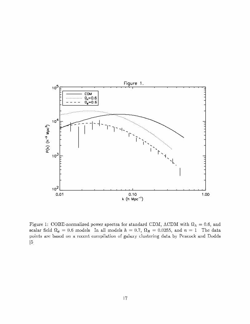
Figure 1: COBE-normalized power spectra for standard CDM, �CDM with � = 0:6, andscalar �eld � = 0:6 models. In all models h = 0:7, B = 0:0255, and n = 1. The datapoints are based on a recent compilation of galaxy clustering data by Peacock and Dodds[5].

17

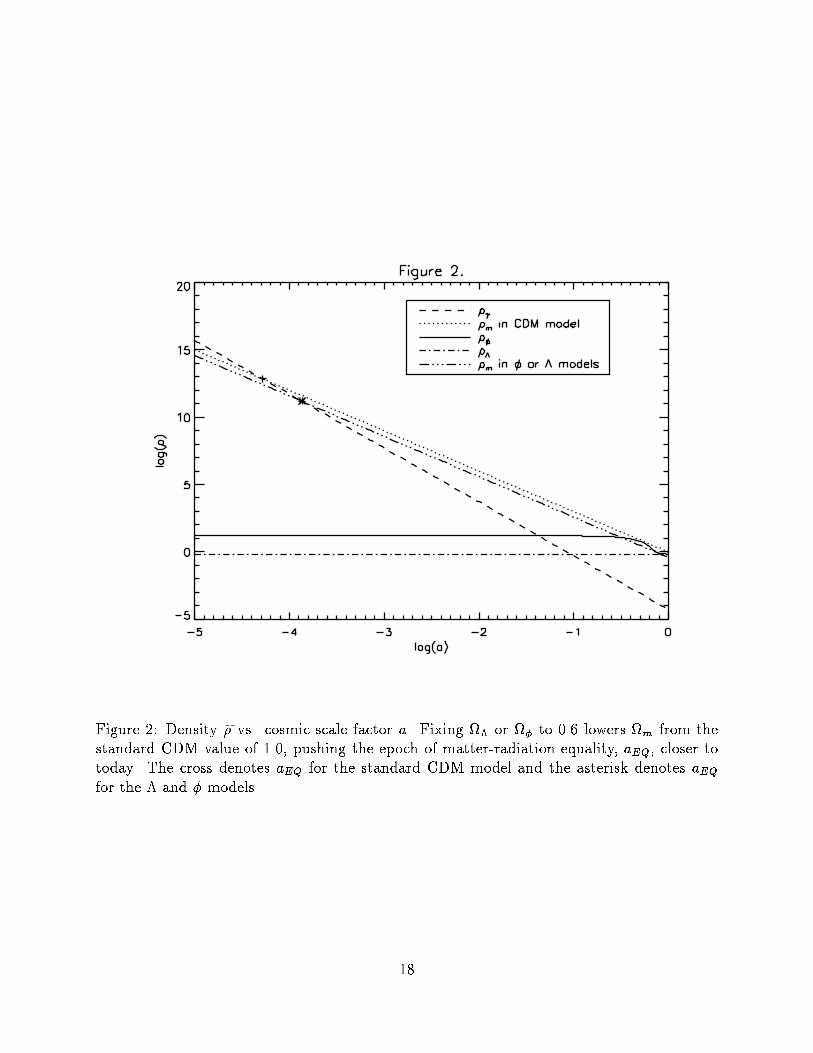
Figure 2: Density �� vs. cosmic scale factor a. Fixing � or � to 0.6 lowers m from thestandard CDM value of 1.0, pushing the epoch of matter-radiation equality, aEQ, closer totoday. The cross denotes aEQ for the standard CDM model and the asterisk denotes aEQfor the � and � models.

18

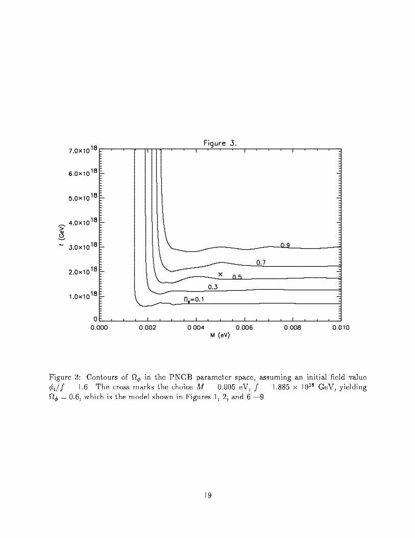
Figure 3: Contours of � in the PNGB parameter space, assuming an initial �eld value�i=f = 1:6. The cross marks the choice M = 0:005 eV, f = 1:885 � 1018 GeV, yielding� = 0:6, which is the model shown in Figures 1, 2, and 6 { 9.

19

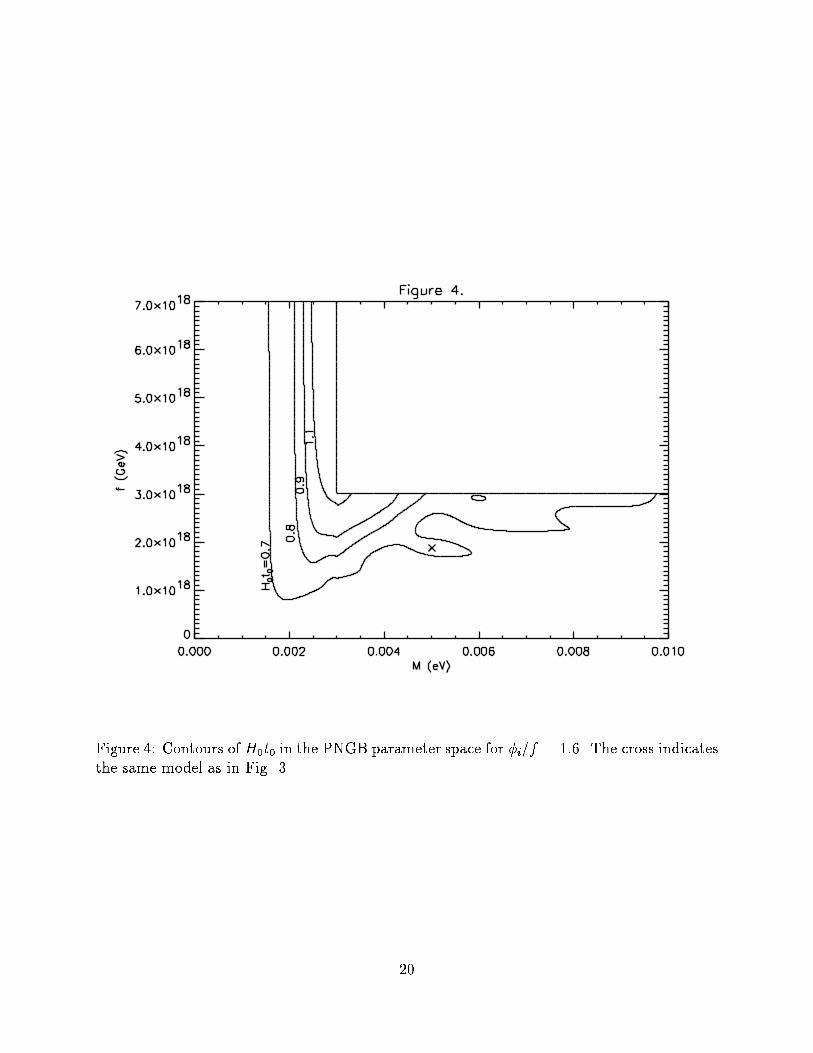
Figure 4: Contours of H0t0 in the PNGB parameter space for �i=f = 1:6. The cross indicatesthe same model as in Fig. 3.

20

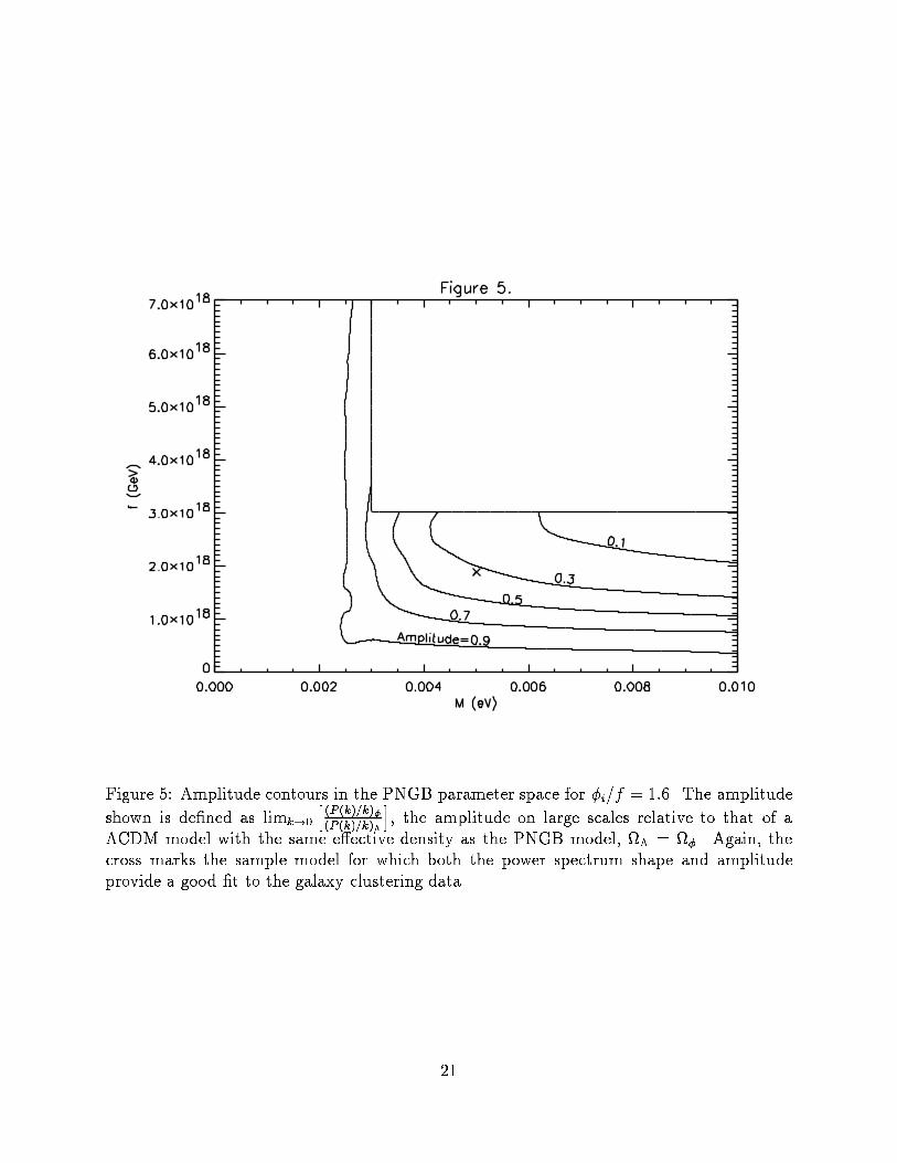
Figure 5: Amplitude contours in the PNGB parameter space for �i=f = 1:6. The amplitude

shown is de�ned as limk!0

h(P (k)=k)�(P (k)=k)�

i, the amplitude on large scales relative to that of a

�CDM model with the same e�ective density as the PNGB model, � = �. Again, thecross marks the sample model for which both the power spectrum shape and amplitudeprovide a good �t to the galaxy clustering data.

21

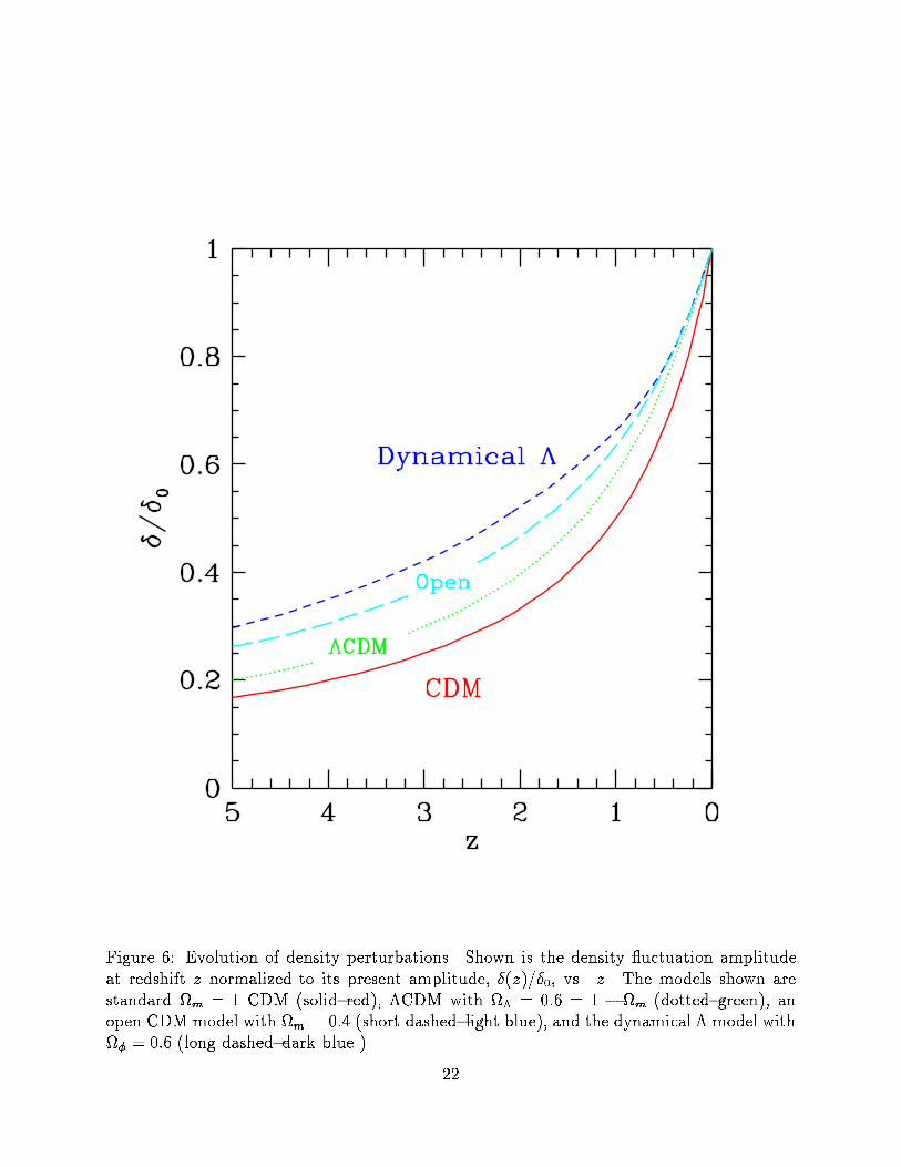
Figure 6: Evolution of density perturbations. Shown is the density uctuation amplitudeat redshift z normalized to its present amplitude, �(z)=�0, vs. z. The models shown arestandard m = 1 CDM (solid{red), �CDM with � = 0:6 = 1 � m (dotted{green), anopen CDM model with m = 0:4 (short dashed{light blue), and the dynamical � model with� = 0:6 (long dashed{dark blue ).

22

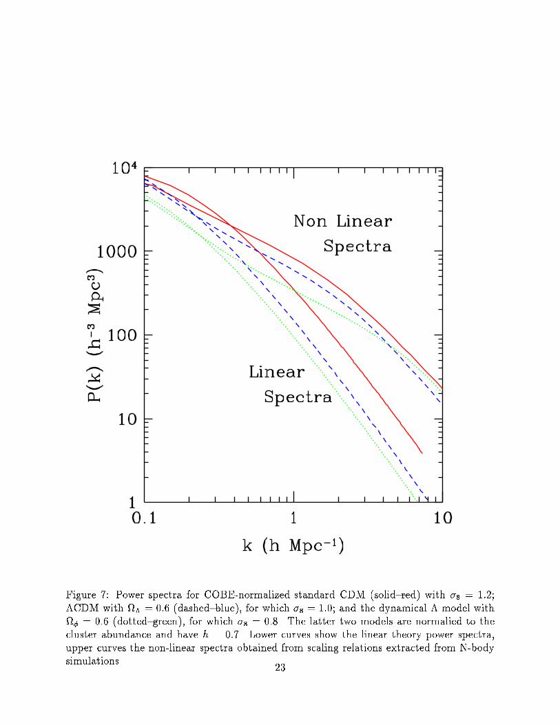
Figure 7: Power spectra for COBE-normalized standard CDM (solid{red) with �8 = 1:2;�CDM with � = 0:6 (dashed{blue), for which �8 = 1:0; and the dynamical � model with� = 0:6 (dotted{green), for which �8 = 0:8. The latter two models are normalied to thecluster abundance and have h = 0:7. Lower curves show the linear theory power spectra,upper curves the non-linear spectra obtained from scaling relations extracted from N-bodysimulations.

23

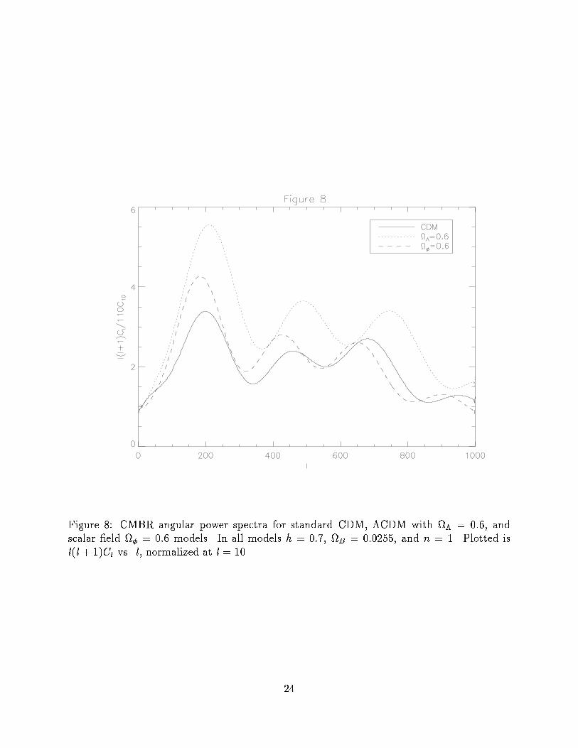
Figure 8: CMBR angular power spectra for standard CDM, �CDM with � = 0:6, andscalar �eld � = 0:6 models. In all models h = 0:7, B = 0:0255, and n = 1. Plotted isl(l+ 1)Cl vs. l, normalized at l = 10.

24

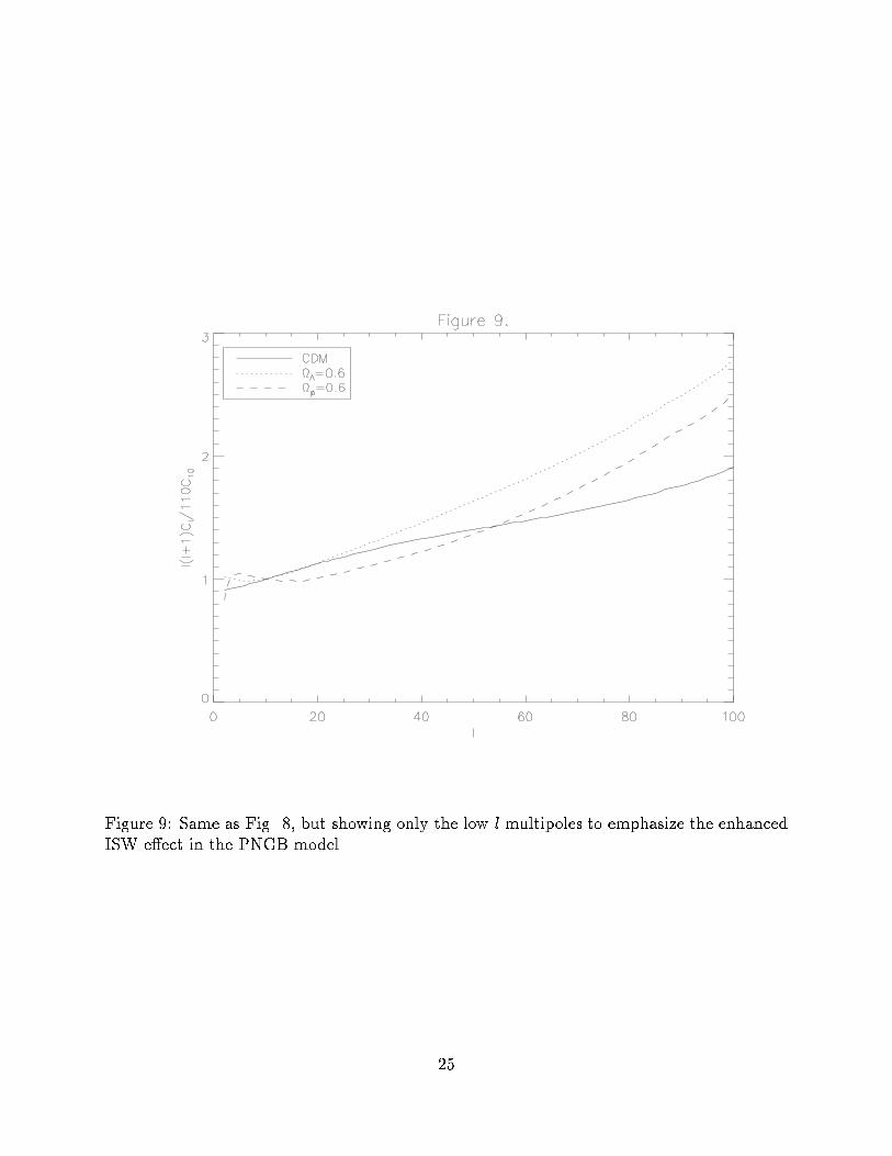
Figure 9: Same as Fig. 8, but showing only the low l multipoles to emphasize the enhancedISW e�ect in the PNGB model.

25