Physica D 157 (2001) 147–165

Dynamical models of phyllotaxis

Martin Kunz∗Eidgenössische Technische Hochschule Zürich, 8092 Zürich, Switzerland

Received 1 June 2000; received in revised form 25 February 2001; accepted 28 March 2001Communicated by J.P. Keener

Abstract

Leave patterns on plants (phyllotaxis) present remarkable universal features. The underlying morphogenesis phenomenoncan be modelled by a class of dynamical systems referred to as inhibitory field models. Numerical studies have shown that,surprisingly often, the fixed points of such systems closely correspond to noble numbers; this is exactly what is observed innature. In the present paper a proof of this fact is given, that applies in particular to the model of Thornley. But the analysis isgeneral enough to embrace all models usually considered: an explicit criterion is given to explain under which circumstancesnoble numbers are actually selected. A stability analysis of the fixed points is also performed, explaining observed bifurcations.© 2001 Elsevier Science B.V. All rights reserved.

Keywords: Morphogenesis; Dynamical systems; Noble numbers

1. Introduction

In this paper, we present a mathematical analysis of dynamical models of phyllotaxis. As explained in the next sec-tion, phyllotaxis refers to the pattern of leaves on a stem (or similar botanical structures), which present in most casesa remarkable regularity. An unexpected and universal feature of these patterns is the role played by the golden mean

τ = 12 (1 +

√5) (1)

in their geometrical description. The search for an explanation of this surprising fact has a long history (see e.g.[1,4,8]). Since the last century and the observations of Hofmeister [7], it has been known that the key to this problemhas to be found in the initial stages of leaves formation. Phyllotaxis can therefore be considered as a simple andnon-trivial instance of morphogenesis in biology. A very important suggestion in this problem has been made byTuring [19], who proposed that pattern formation is the result of a spatial instability in a reaction–diffusion system.Needless to say, one should be very cautious when discussing the relevance of such ideas to real growth process: inthe realm of living organisms, any theory is certainly bound to leave in the shadow the greatest part of the Creator’swork! There is actually no direct evidence that Turing’s mechanism is at work in nature, in particular in phyllotaxis.Nevertheless, inspired by Turing, several authors have proposed discrete time dynamical models of phyllotaxis,known as inhibitory field models; a numerical analysis of these dynamical systems shows a close analogy with the

∗ Present address: Village 35, CH-1066 Epalinges, Switzerland.

0167-2789/01/$ – see front matter © 2001 Elsevier Science B.V. All rights reserved.PII: S0 1 6 7 -2 7 89 (01 )00275 -5

148 M. Kunz / Physica D 157 (2001) 147–165

observed biological patterns (see e.g. [3,10,14,15,18,27]). Moreover, it has been shown that these models actuallyfit in Turing’s reaction–diffusion framework [2]. The inhibitory field theory provides thus an internally consistentpicture of the phenomenon, even if the true mechanism at work in nature remains to be uncovered.

Inhibitory field model provide thus an interesting empirical approach to phyllotaxis; however, their behaviour hasremained obscure from a mathematical standpoint, at least for chemical models such as Thornley’s model [18,27]or Bernasconi reaction–diffusion system [2]. The aim of this paper is to provide a rigorous analysis that applies tosuch cases. For the first time, a general criterion is given for the selection of the golden mean by such dynamicalsystems. A stability analysis of the stationary solutions is also performed, yielding explicit formulae for the variousbifurcations encountered in numerical computations [5,9,22,23].

The paper is organised as follows: in Section 2, a short introduction to the phenomenon of phyllotaxis is given.Section 3 presents some examples of inhibitory field models; special emphasis is put on Thornley’s model, sinceour analysis was initially developed to explain its properties. But the approach is valid in a much broader context:the geometrical picture of field models is therefore presented in general terms. This representation is put to workin Section 4, where the main results are presented. Again, Thornley’s model is treated into greater detail: Theorem3 is an application of the results to this special case, and the conditions under which noble numbers are selectedare fully elucidated. Finally, Section 5 is devoted to a stability analysis of stationary solutions. The geometricalrepresentation of Section 3 also proves useful in this context.

2. Phyllotaxis as a morphogenesis process

Phyllotaxis refers to the arrangement of leaves on a stem, scales on a fir cone, florets on a daisy or a sunflower,and so on. These botanical elements form a lattice characterised by the nearly systematic appearance of Fibonaccinumbers (see e.g. [8]). Rather than describing these macroscopic patterns, we shall briefly sketch the underlyingprocess of cellular growth and differentiation (for more detailed information, see [13,17,21]). From this point ofview, phyllotaxis is a morphogenesis phenomenon and can possibly be described as a dynamical system.

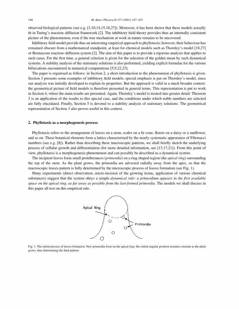
The incipient leaves form small protuberances (primordia) on a ring shaped region (the apical ring) surroundingthe top of the stem. As the plant grows, the primordia are advected radially away from the apex, so that themacroscopic leaves pattern is fully determined by the microscopic process of leaves formation (see Fig. 1).

Many experiments (direct observation, micro-incision of the growing tissue, application of various chemicalsubstances) suggest that the system obeys a simple dynamical rule: a primordium appears in the first availablespace on the apical ring, as far away as possible from the last-formed primordia. The models we shall discuss inthis paper all rest on this empirical rule.

Fig. 1. The initial process of leaves formation. New primordia form on the apical ring: this initial angular position remains constant as the plantgrows, thus determining the final pattern.

M. Kunz / Physica D 157 (2001) 147–165 149

The appearance of Fibonacci numbers in the pattern of leaves is a direct consequence of the following fact: thedivergence 0 ≤ θ < 1 (fraction of the stem circumference) between two consecutive primordia on the apical ringis constant and is close to the golden mean

θF = τ − 1 = 0.618034 . . . . (2)

The connection between phyllotaxis and number theory rests on the arithmetical nature of τ , which is the simplestalgebraic number of degree two:

τ 2 − τ − 1 = 0. (3)

All remarkable properties of τ can be related to its continued fraction expansion

θF = τ − 1 = 1

1 + 11+ 1

1+···

= [1, 1, 1, . . . ]. (4)

Generally speaking, numbers whose continued fraction expansion finishes with an infinite sequence of units arecalled noble numbers. Surprisingly, when the golden divergence is not observed, the angular distance betweensuccessive leaves is close to some other simple noble number:

[3, 1, 1, . . . ] = 0.2764 . . . (Lucas divergence)

[4, 1, 1, . . . ] = 0.2166 . . .

[2, 2, 1, 1, . . . ] = 0.4198 . . .

[2, 3, 1, 1, . . . ] = 0.4393 . . .

[3, 2, 1, 1, . . . ] = 0.2957 . . .

. . .

(5)

The divergence may also simply equal 12 (distichous phyllotaxis), or take alternatively two values:

12 ,

14 ,

12 ,

14 , . . . (decussate phyllotaxis), 1

2 ,12θF,

12 ,

12θF . . . (bijuguate phyllotaxis). (6)

With the exception of decussate and distichous phyllotaxis, which occur systematically in given species, all theabove cases can be considered as highly uncommon. For a detailed exposition, we refer to [8].

3. Inhibitory field models of phyllotaxis

3.1. Definition and examples

In order to account for the appearance of new leaves on the stem, many authors (see the examples below) havepostulated the existence of an inhibitory field F(x, t), where 0 ≤ x < 1 is the coordinate of a point on the apicalring and t the time elapsed since the youngest leaf has appeared. The field is obtained by superposing the inhibitoryeffect of all existing leaves:

F(x, t) = f (x − y1, t)+N∑n=2

f (x − yn, t + t1 + · · · + tn−1). (7)

Here yn represents the point on the apical ring where the nth leaf has appeared (the first leaf being the youngest); tiis the time elapsed between the appearance of leaves i and i + 1 (plastochrone). We may either let N go to infinityas new leaves are introduced, or fix a maximal value of N and forget about the oldest leaves.

150 M. Kunz / Physica D 157 (2001) 147–165

The choice of the function f is to a great extent arbitrary; for the time being, we shall simply assume that f (x, t)is a strictly decreasing function of t and x ∈ (0, 1

2 ), and f (x, t) = f (−x, t) = f (x + 1, t). We shall also assumethat f is twice continuously differentiable in x and t , except for a possible cusp at x = 0 (we shall assume boundedderivatives in this case). Any additional precision calls for a specific model of the biological, physical or chemicalmechanisms involved in the growth process. The interesting point, as we shall see, is that general conclusions canbe drawn irrespective of the exact form of f .

Two kinds of models are considered: one may either suppose that the plastochrone ti = T is a constant andput the new leaf at the absolute minimum of F(x, T ) (constant plastochrone systems), or decide that the new leafappears as soon as F(x, t) reaches some threshold value F0 at some point x (threshold systems). WhenN is fixed, aconstant plastochrone system defines a piecewise continuous map of the (N − 1)-torus T N−1 onto itself; similarly,the phase space of a threshold system is the product T N−1 × RN−1

+ (see Section 5 for a further discussion of thesemaps). In both systems stationary solutions, which correspond to a constant divergence θ , are such that

ti = T , yn+1 − yn = θ. (8)

The model provides a correct description of the growth process if, under appropriate initial conditions, a stationaryregime with a typical divergence (e.g. θ θF) is reached.

Since they are in qualitative agreement with the dynamical rule explained in the preceding section, inhibitory fieldmodels provide an attractive synthesis of various experimental facts relating to the growth process. Although the veryexistence of an inhibitory field remains hypothetical, these models offer an effective description of the phenomenon.All observed structures of leaves, to the knowledge of the author, can be reproduced within a field model (see forinstance [5,22,23]); conversely, there are simple structures which obviously contradict the field hypothesis and arenever observed in nature. For instance, there exists no plant exhibiting opposite distichous phyllotaxis (pairs ofopposite leaves, each pair being above the other).

It is worthy to note that these models do not constitute, by themselves, a theory of morphogenesis, insofar asthe inhibitory field does not obey a local equation of motion. One may therefore ask: is there a way to derive theabove dynamical system from the evolution equations of some physical and/or chemical system? As a matter offact, the phenomenon of differentiation and self-organisation of the tissue is largely unknown and must involvecomplex physical, chemical or biological processes. Now Turing [19] has conjectured that morphogenesis resultsfrom spontaneous pattern formation in the concentration fields of morphogenes, i.e. chemical substances reactingand diffusing in the tissue and responsible for the differentiation of cells. Such an hypothesis is of course extremelydifficult to prove (or disprove) experimentally; nevertheless, it probably reveals a simple and fundamental process. Italso provides a natural framework for inhibitory field models: it is possible to construct a simple reaction–diffusionsystem on the apical ring reproducing, in a suitable limit, the behaviour of an inhibitory field model [2,9]; from thispoint of view, the inhibitory field may be considered as a morphogene.

Before we present some specific field models, which were constructed along various lines of reasoning, let usdefine an important concept for the analysis of these systems. Consider first a threshold system. The threshold F0

is a free parameter that enables the definition of the divergence spectrum

∆0 = (F0, θ) : there exists a stationary solution with divergence θ and thresholdF0. (9)

In the case of a constant plastochrone system, the plastochrone T is the natural parameter. The divergence spectrumis the set

∆0 = (T , θ) : there exists a stationary solution with divergence θ and plastochrone T . (10)

The main fact relative to inhibitory field models of phyllotaxis is that surprisingly often, the spectrum consistsin curves approaching the golden mean, Lucas number or other noble numbers on the θ -axis as T → 0 (or F0

M. Kunz / Physica D 157 (2001) 147–165 151

increases). The spectrum is therefore the natural object to consider in order to understand the role played by noblenumbers. This point will be illustrated with the following examples.

Example A: Thornley’s model. In this model, the plastochrone equals one and

f (x, t) = λtf (x), (11)

where λ ∈ (0, 1) is the free parameter [10,14,18,27]. It is of course completely equivalent to pick some λ0 ∈ (0, 1)and consider T ∈ (0,∞) as the parameter, with

λT0 = λ. (12)

For an apparently broad class of functions f , the spectrum displays an accurate selection of the golden mean andother noble numbers. The basic mathematical problem is to determine this class of functions and the accuracy withwhich noble numbers are selected.

Example B: Douady and Couder experiment. These authors devised a physical experiment which can be formallydescribed by an inhibitory field model. Droplets of ferrofluid lie in a disc filled with a viscous fluid. A new dropletis periodically introduced in the system, on the top of a small hemisphere placed at the centre of the disc. Anon-uniform magnetic field is applied, which causes outward radial motion of the droplets; moreover, the newlyintroduced droplet is repelled by the others, so that it reaches the boundary of the hemisphere at the point where theresulting potential is minimum. In a stationary regime, the divergence between successive particles on the boundaryof the hemisphere is constant. The divergence spectrum gives the set of stationary divergences for all values of theplastochrone T .

Douady and Couder obtained such a spectrum by a numerical computation [3]; it has a striking auto-similarstructure, each branch leading to a noble divergence as T tends towards 0. Douady and Couder noticed its closeanalogy with the Farey tree and put forward a geometrical argument to explain this structure. We shall return to thispoint later.

Example C: Koch–Bernasconi–Rothen model. This model was devised to reproduce the behaviour of the “source”field in the reaction–diffusion system of Bernasconi and co-workers [9]. The field due to an individual leaf is

f (x, t) = e−t∞∑

n=−∞e−(x−n)2/2σ 2

. (13)

The threshold value F0 is an independent parameter which determines the plastochrone and can be related toparameters of the reaction–diffusion system. If σ is small enough, noble numbers are accurately selected.

3.2. Geometrical interpretation of the models

We present now the central idea of this paper, which shows that Example B is in a sense universal. We assumethat the inhibitory field f (x, t) created by an individual leaf can be written as

f (x, t) = V [δ(x,Φ(t))], (14)

where Φ(t) ≥ 1 is a strictly increasing function of t and V is a decreasing function. δ must have the followingproperties, which follow from the properties of f : δ(x,Φ) is a strictly increasing function of x ∈ (0, 1

2 ) andΦ, andδ(x,Φ) = δ(−x,Φ) = δ(x + 1, Φ). Moreover, all these functions are twice continuously differentiable, exceptfor a possible cusp of δ at x = 0 (in this case derivatives are bounded).

We can adopt a geometrical point of view, from which this formulation appears as very natural. Suppose that theyoung leaves can be identified with particles lying on some surface S of revolution, homeomorphic to a half-infinite

152 M. Kunz / Physica D 157 (2001) 147–165

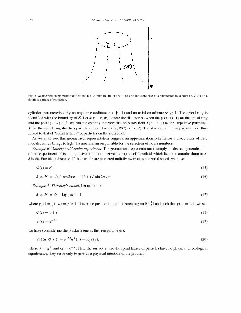
Fig. 2. Geometrical interpretation of field models. A primordium of age t and angular coordinate y is represented by a point (y,Φ(t)) on afictitious surface of revolution.

cylinder, parameterised by an angular coordinate x ∈ [0, 1) and an axial coordinate Φ ≥ 1. The apical ring isidentified with the boundary of S. Let δ(x − y,Φ) denote the distance between the point (x, 1) on the apical ringand the point (y,Φ) ∈ S. We can consistently interpret the inhibitory field f (x − y, t) as the “repulsive potential”V on the apical ring due to a particle of coordinates (y,Φ(t)) (Fig. 2). The study of stationary solutions is thuslinked to that of “spiral lattices” of particles on the surface S.

As we shall see, this geometrical representation suggests an approximation scheme for a broad class of fieldmodels, which brings to light the mechanism responsible for the selection of noble numbers.

Example B: Douady and Couder experiment. The geometrical representation is simply an abstract generalisationof this experiment. V is the repulsive interaction between droplets of ferrofluid which lie on an annular domain S.δ is the Euclidean distance. If the particle are advected radially away at exponential speed, we have

Φ(t) = et , (15)

δ(u,Φ) =√(Φ cos 2πu− 1)2 + (Φ sin 2πu)2. (16)

Example A: Thornley’s model. Let us define

δ(u,Φ) = Φ − log g(u)− 1, (17)

where g(u) = g(−u) = g(u+ 1) is some positive function decreasing on [0, 12 ] and such that g(0) = 1. If we set

Φ(t) = 1 + t, (18)

V (r) = e−Kr (19)

we have (considering the plastochrone as the free parameter):

V [δ(u,Φ(t))] = e−KtgK(u) = λt0f (u), (20)

where f = gK and λ0 = e−K . Here the surface S and the spiral lattice of particles have no physical or biologicalsignificance; they serve only to give us a physical intuition of the problem.

M. Kunz / Physica D 157 (2001) 147–165 153

4. Hierarchical selection of noble numbers

We shall explain the properties of the divergence spectrum relating to noble numbers on the basis of a nearestneighbours approximation. This approximation, which follows from the geometrical representation described inthe preceding section, is implicitly used in the arguments given in [3,4,15,16,26] in the framework of physical orgeometrical models of phyllotaxis. Our general analysis puts the argument on a firm basis and shows its generality.In particular, we will obtain a criterion for the selection of noble numbers in Thornley’s and similar “chemical”models, for which no analytical understanding was so far available.

For the sake of simplicity, we restrict our analysis to constant plastochrone systems. We shall demonstrate inAppendix A how the results extend naturally to threshold systems. Assume that the (real or fictitious) potential Vintroduced in Section 3.2 has the form

V (r) = e−Kr, (21)

K is an additional parameter; we will examine the consequences of taking the limit K → ∞. Other choices ofV can be made, insofar as the interaction decreases sufficiently fast in the limit K → ∞. Consider a stationarysolution; the resulting inhibitory field reads

F(x, T ) =N∑n=1

V [δ(x − nθ, Φ(nT))] =N∑j=1

V [δj (x)], (22)

where

δj (x) = δ[x − σ(j)θ, Φ(σ(j)T )] (23)

and σ is a permutation defined so that δj (0) ≤ δj+1(0).By definition of the model

F(0, T ) ≤ F(x, T ) ∀x. (24)

We shall restrict ourselves to the weaker condition

∂xF (0, T ) = 0, (25)

which defines a spectrum ∆ ⊃ ∆0. This relaxed constraint, first proposed by Guerreiro [6,24], simplifies greatlythe analysis; moreover, the selection of noble numbers basically depends on the properties of ∆. The relationshipbetween ∆ and ∆0 has been discussed in a general context by Guerreiro; we shall come back to this aspect of theproblem later.

Let us assume that δ has no cusp at x = 0 (if this is not the case, one can first smoothen δ in an ε-neighbourhoodof x = 0 and then take ε → 0 in the end; this is allowed since δ has bounded derivatives and is differentiated onlyonce in the following computation). We can write

0 = ∂xF (0, T ) =N∑n=1

−K e−Kδn(0) ∂δn∂x(0) ∝ ∂δ1

∂x+ e−K(δ2−δ1)r, (26)

where

r =N∑n=2

e−K(δn−δ2) ∂δn∂x

(27)

154 M. Kunz / Physica D 157 (2001) 147–165

is bounded from above by a decreasing function of K . Obviously, if |∂xδ1| > ε1 and |δ2 − δ1| > ε2, then ∂xF = 0if K is great enough. Thus in the limit K → ∞, the spectrum ∆ is necessarily included in a neighbourhood of theset

Σ" =(T , θ) ∈ (0,∞)× [0, 1) : δ1 = δ2 or

∂δ1

∂x= 0

, (28)

which depends only on the local structure of the “spiral lattice” of leaves. The problem amounts thus to a geometricalstudy of this lattice.

With rather general assumptions on the functions δ and Φ, it is possible to prove that Σ" has the structure of theFarey tree. Let us explain what we mean by this: the set

Σ = (T , θ) : δ1 = δ2 (29)

is an union of continuous lines (branches) in the (T , θ)-plane, each branch being the implicit solution of

δ1(0) = δ2(0), σ (1) = n, σ (2) = m. (30)

Such a branch is labelled by the integers (n,m) (n < m). Each (n,m) branch can be continued until it reachesa bifurcation point δ1 = δ2 = δ3. At this point, it is connected to two other branches, one of which is regular((m, n + m)-branch) and the other singular ((n, n + m)-branch). σ(1) is always a decreasing function of T , sothat regular and singular branches are easily distinguished on a graphical representation of Σ . Each branch canbe reached starting from (n = 1,m = 2). Σ is invariant under the reflexion θ → 1 − θ , and the branch (1, 2)always cuts the symmetry axis θ = 1

2 . Moreover, there is a close connection betweenΣ and the continued fractionexpansion of the divergence

θ = 1

a1 + 1a2+ 1

a3+···

= [a1, a2, a3, . . . ]. (31)

If (T , θ) ∈ (n,m), then for some k ∈ N

n = qk,m = qk+1 or qk+2, (32)

where the irreducible fractionspj

qj= [a1, a2, . . . , aj ] (33)

are the principal convergents of θ .When possessing all these properties, the setΣ is said to have the Farey tree structure. The setΣ" is then simply

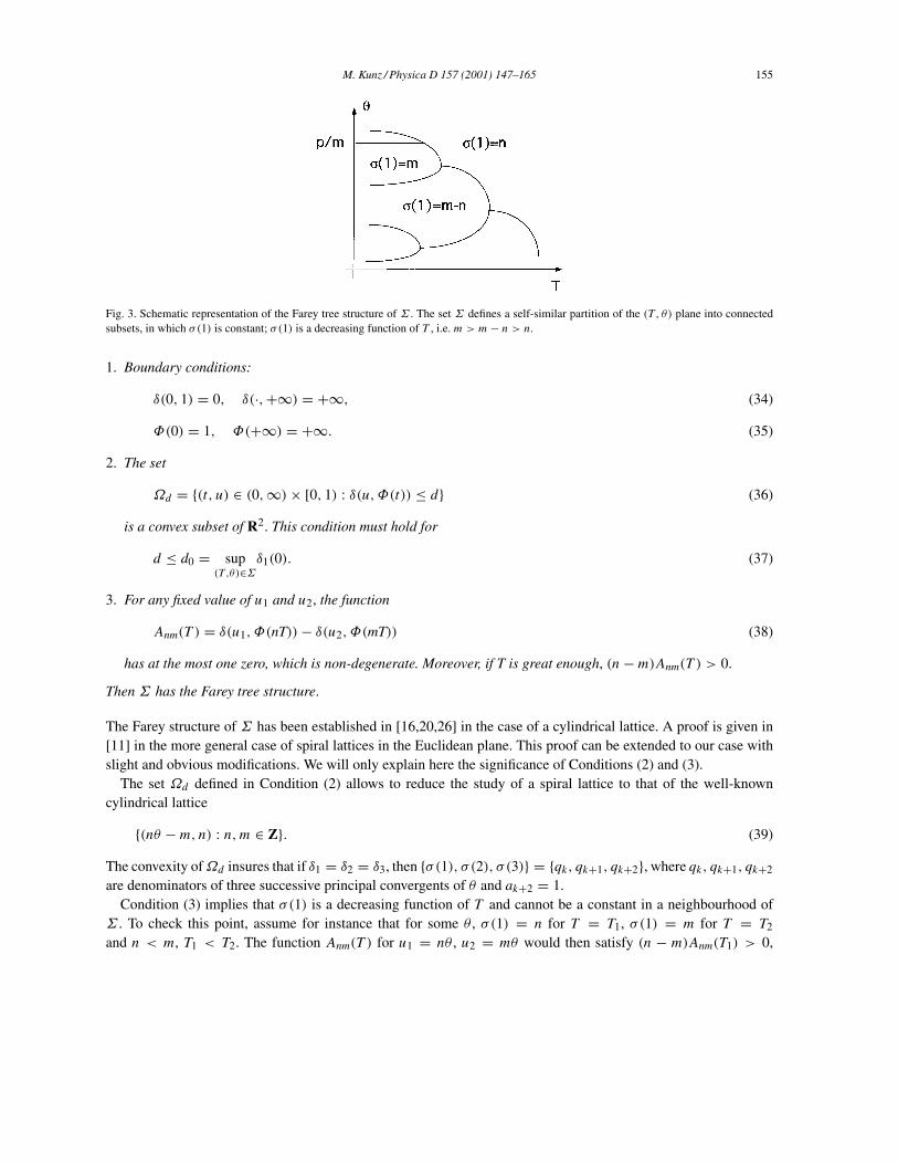
obtained by adding segments θ = p/m, p ∈ N, connected to singular branches (n,m) ∈ Σ (Fig. 3).The most important property ofΣ is that it provides a graphical representation of the continued fraction expansion.

As a matter of fact, if (T , θ) ∈ Σ , there exists an unique path in Σ connecting the axis θ = 12 to (T , θ): the first

partial quotients of θ are then determined by the sequence of regular and singular branches constituting this path:ai − 1 is the number of singular branches preceding the ith regular branch in the path. 1 Thus any path whichfinishes with an infinite sequence of regular branches cuts the axis T = 0 at a noble number θ . Conversely, rationaldivergences are reached by an infinite sequence of singular branches.

We now state a theorem which says precisely under which circumstances Σ has the Farey tree structure.

Theorem 1. Suppose that δ and Φ satisfy the following conditions:

1 If we agree upon the following understanding: the first regular branch is (1, 2) if θ ∈] 12 , 1[ and (n, n+ 1) (n ≥ 2) if θ ∈]0, 1

2 [.

M. Kunz / Physica D 157 (2001) 147–165 155

Fig. 3. Schematic representation of the Farey tree structure of Σ . The set Σ defines a self-similar partition of the (T , θ) plane into connectedsubsets, in which σ(1) is constant; σ(1) is a decreasing function of T , i.e. m > m− n > n.

1. Boundary conditions:

δ(0, 1) = 0, δ(·,+∞) = +∞, (34)

Φ(0) = 1, Φ(+∞) = +∞. (35)

2. The set

Ωd = (t, u) ∈ (0,∞)× [0, 1) : δ(u,Φ(t)) ≤ d (36)

is a convex subset of R2. This condition must hold for

d ≤ d0 = sup(T ,θ)∈Σ

δ1(0). (37)

3. For any fixed value of u1 and u2, the function

Anm(T ) = δ(u1, Φ(nT))− δ(u2, Φ(mT)) (38)

has at the most one zero, which is non-degenerate. Moreover, if T is great enough, (n−m)Anm(T ) > 0.

Then Σ has the Farey tree structure.

The Farey structure of Σ has been established in [16,20,26] in the case of a cylindrical lattice. A proof is given in[11] in the more general case of spiral lattices in the Euclidean plane. This proof can be extended to our case withslight and obvious modifications. We will only explain here the significance of Conditions (2) and (3).

The set Ωd defined in Condition (2) allows to reduce the study of a spiral lattice to that of the well-knowncylindrical lattice

(nθ −m, n) : n,m ∈ Z. (39)

The convexity ofΩd insures that if δ1 = δ2 = δ3, then σ(1), σ (2), σ (3) = qk, qk+1, qk+2, where qk, qk+1, qk+2

are denominators of three successive principal convergents of θ and ak+2 = 1.Condition (3) implies that σ(1) is a decreasing function of T and cannot be a constant in a neighbourhood of

Σ . To check this point, assume for instance that for some θ , σ(1) = n for T = T1, σ(1) = m for T = T2

and n < m, T1 < T2. The function Anm(T ) for u1 = nθ , u2 = mθ would then satisfy (n − m)Anm(T1) > 0,

156 M. Kunz / Physica D 157 (2001) 147–165

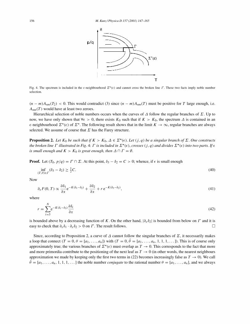
Fig. 4. The spectrum is included in the ε-neighbourhood Σ"(ε) and cannot cross the broken line Γ . These two facts imply noble numberselection.

(n − m)Anm(T2) < 0. This would contradict (3) since (n − m)Anm(T ) must be positive for T large enough, i.e.Anm(T ) would have at least two zeroes.

Hierarchical selection of noble numbers occurs when the curves of ∆ follow the regular branches of Σ . Up tonow, we have only shown that ∀ε > 0, there exists K0 such that if K > K0, the spectrum ∆ is contained in anε-neighbourhood Σ"(ε) of Σ". The following result shows that in the limit K → ∞, regular branches are alwaysselected. We assume of course that Σ has the Farey structure.

Proposition 2. Let K0 be such that if K > K0, ∆ ∈ Σ"(ε). Let (j, q) be a singular branch of Σ . One constructsthe broken line Γ illustrated in Fig. 4: Γ is included inΣ"(ε), crosses (j, q) and dividesΣ"(ε) into two parts. If εis small enough and K > K0 is great enough, then ∆ ∩ Γ = ∅.

Proof. Let (T0, p/q) = Γ ∩Σ . At this point, δ3 − δ2 = C > 0; whence, if ε is small enough

inf(T ,θ)∈Γ

(δ3 − δ2) ≥ 12C. (40)

Now

∂xF (0, T ) ∝ ∂δ1

∂xe−K(δ1−δ2) + ∂δ2

∂x+ r e−K(δ3−δ2), (41)

where

r =N∑i=3

e−K(δi−δ3) ∂δi∂x

(42)

is bounded above by a decreasing function of K . On the other hand, |∂xδ2| is bounded from below on Γ and it iseasy to check that ∂xδ1 · ∂xδ2 > 0 on Γ . The result follows.

Since, according to Proposition 2, a curve of ∆ cannot follow the singular branches of Σ , it necessarily makesa loop that connect (T = 0, θ = [a1, . . . , an]) with (T = 0, θ = [a1, . . . , an, 1, 1, 1, . . . ]). This is of course onlyapproximately true; the various branches of Σ"(ε) must overlap as T → 0. This corresponds to the fact that moreand more primordia contribute to the positioning of the next leaf as T → 0 (in other words, the nearest neighboursapproximation we made by keeping only the first two terms in (22) becomes increasingly false as T → 0). We callθ = [a1, . . . , an, 1, 1, 1, . . . ] the noble number conjugate to the rational number θ = [a1, . . . , an], and we always

M. Kunz / Physica D 157 (2001) 147–165 157

assume 2 an > 1. Of course, because of the symmetry θ → 1 − θ , there is a bifurcation at θ = 12 = [2] (one loop

leads to [1, 1, 1, . . . ] and the other to [2, 1, 1, . . . ]).It remains to discuss the relationship between∆ and∆0. The following terminology will be useful: in the region

where branches do not overlap and Proposition 2 applies, each loop can be decomposed into a straight part and anoscillating part, the first one being included in the ε-neighbourhood of the set Σ" \Σ (in other words, the straightpart leads to a rational divergence and the oscillating part leads to the conjugate noble number). If the lattice iscylindrical it can be shown, in the limit K → ∞, that ∆0 consists in the oscillating parts of the curves of ∆ [11];this situation is also observed (although with finite accuracy) in the spectrum obtained by Douady and Couder[3]. It is not easy to generalise this result; ∆0 may contain only a fraction of the oscillating curves, as numericalexamples show [6,24]. On the other hand, as we shall see, the straight parts are always excluded from the spectrumof dynamically stable solutions.

To conclude this section, we apply our results to Thornley’s model and state the following theorem, which givesa simple criterion insuring that noble numbers are selected. As explained above, it is necessary to consider a familyof systems, depending on the parameterK , and to study the limitK → ∞. We focus on Thornley’s system becausethus far, no analytical explanation for the selection of noble numbers in this model had been given. Similar theoremsare stated in [11] for Douady–Couder models. We use the plastochrone T instead of the traditional parameter λ; inthis way the natural structure of the problem appears more clearly (the spectra “converge” towards a “geometricalspectrum” in the limit K → ∞). For each value of K , we can pass from one parameter to the other using theformula

λ = e−KT. (43)

Theorem 3 (Thornley’s model). Consider the one-parameter family of Thornley’s models defined by the functions

fK(x) = gK(x) (44)

so that the inhibitory field for a constant divergence θ is

FT,θ,K(x) =∑n≥1

e−nKTfK(x − nθ). (45)

Assume that g is logarithmically convex (i.e. log g is concave) in the interval g(x) ≥ e−d0 , where d0 is definedaccording to (37) and depends only on g.

Then for any rational divergence θ0 = p/q and any ε > 0, there exists K0 such that ∀K ≥ K0, the spectrum

∆0(K) = (T , θ) ∈ (0,∞)× [0, 1) : ∂xFT,θ,K(0) = 0 (46)

contains a continuous curve joining (T (ε), θ0 + s) and (T (ε), θ0 + s′) where θ0 is the noble number conjugate toθ0, |s|, |s′| < ε and limε→0T (ε) = 0. Moreover, the above curves do not intersect and follow the branches of aFarey tree.

Proof. This theorem is a direct consequence of Theorem 1, Proposition 2 and the above discussion. Let us brieflyreview the main steps of the reasoning: first we define a distance δ and a function Φ according to (17) and (18).These definitions depend only on g and not on the parameters T and K . According to (20) we can now interpretthe inhibitory field FT,θ,K(x) as the potential created by particles placed on a “spiral lattice”. This lattice is entirely

2 A finite continued fraction can always be written in two ways: [a1, . . . , an] = [a1, . . . , an − 1, 1].

158 M. Kunz / Physica D 157 (2001) 147–165

defined by g, T and θ ; moreover, these “geometrical” parameters are independent from the potential V and theparameter K .

We can now construct the sets Σ and Σ" according to the definitions (28) and (29). This is a purely geometricalproblem. It is straightforward to verify that all conditions of Theorem 1 are satisfied (Condition (2) follows fromthe log convexity of g). The set Σ" therefore has the Farey tree structure.

We pick now some small ε > 0 and construct the 12ε-neighbourhoods Σ( 1

2ε), Σ"( 1

2ε) of Σ , Σ". We restrictourselves to the region

Ω = (T , θ) : 0 < T ≤ T0, 0 ≤ θ < 1, (47)

where T0 (independent of ε, K) has been chosen so that Σ( 12ε) is entirely contained inΩ . The complementary set

Λ = Ω \Σ"( 12ε) is compact (because branches of Σ"( 1

2ε) overlap as ε → 0); consequently,

inf(T ,θ)∈Λ

(δ2 − δ1) = C0(ε) > 0. (48)

Using (26) and the boundedness of the derivatives of δ, this implies the existence ofK0(ε) such that∆0(K)∩Λ = ∅for allK ≥ K0(ε). If ε is small enough, one can chooseT (ε) > 0 and restrict ourselves to the regionT (ε) ≤ T ≤ T0,so that the branch ofΣ"( 1

2ε) that starts at the rational divergence θ0 = p/q and ends at θ0 does not cover any otherbranch of Σ"( 1

2ε); choosing ε sufficiently small and K0(ε) sufficiently large, Proposition 2 can be applied alongthis whole branch. As a result, we obtain two non-intersecting curves γ1, γ2 whose end points are, respectively,(T (ε), θ0 + 1

2ε), (T (ε), θ (ε)− 12ε) and (T (ε), θ0 − 1

2ε), (T (ε), θ (ε)+ 12ε) (where (T (ε), θ (ε)) ∈ Σ), along which

∂xF (0) never cancels. Moreover, for ε small enough

|θ (ε)− θ0| < 12ε. (49)

Now if ε is small enough, ∂xF (0) has a different sign on γ1 and γ2 since

−eKδ1

K∂xFT (ε),θ0±ε/2,K(0) = ∂δ1

∂x(0)+ O(e−K0C0) (50)

= (−log g)′(q

(θ0 ± ε

2

))+ O(e−K0C0) (51)

= −g′(±qε/2)g(±qε/2) + O(e−K0C0). (52)

This implies the existence of a continuous curve belonging to the spectrum ∆0(K), K ≥ K0(ε), whose end pointsare (T (ε), θ0 + s), (T (ε), θ0 + s′) and |s|, |s′| < ε. The theorem is proved.

Several functions g satisfying the conditions of the theorem can be constructed. For instance

g(x) = 12 (1 + cos 2πx), (53)

g(x) = 4(x − 12 )

2. (54)

This last function had been considered in [10]; the authors studied the case K = 1, where analytical computationsare possible but noble numbers are not selected. Our theorem shows that this selection will indeed occur withincreasing accuracy as K grows to infinity.

It is perhaps useful to explain how the above analysis applies when f is of the form

f (x) =∑n∈Z

hK(x + n) (55)

M. Kunz / Physica D 157 (2001) 147–165 159

andK → ∞. Here h is logarithmically convex but not periodic; for instance h is a Gaussian in the model of Koch,Bernasconi and Rothen (see (13)). In this case it is simpler to consider a periodic lattice in the plane (instead of acylinder), and to define the distance δ according to (17) with g replaced by h.

5. Stability analysis

The aim of this section is to develop a local stability analysis for inhibitory field models. The results will beused to demonstrate the stability of stationary solutions under appropriate conditions. Such an analysis is also thestarting point for the study of bifurcations. As an example, let us mention the subharmonic bifurcations observed in[5,9,22,23] in threshold systems; it is of botanical interest, since it describes a transition from Fibonacci to decussatephyllotaxis.

Field models will be considered as finite dimensional, discrete time dynamical systems. This point of view isquestionable as far as reaction–diffusion models are concerned, since the fluctuations of a chemical concentrationfield define an infinite dimensional space. It should be pointed out, however, that the biological system itself isconstituted of a finite number of cells, so that in this case also it might be necessary to consider a finite dimensionalspace (e.g. a finite number of Fourier components).

We shall distinguish one class of models from the other (constant plastochrone and threshold systems). Anystationary solution of a constant plastochrone system is also a stationary solution of a threshold system; however,it may be stable in one case and unstable in the other.

5.1. Constant plastochrone systems

If the N last primordia are taken into account (N fixed), the inhibitory field F at time t = T is

F(x) =N∑n=1

fn(x − yn). (56)

Here fn denotes the field created by a primordium appeared at time (1 − n)T at yn on the apical ring. Let yN = 0.F can be entirely specified by the vector of divergences

X = (x1, . . . , xN−1), (57)

where

yk = yk+1 + xk. (58)

We can thus denote the inhibitory field at time T by FX. The next primordium will appear at the absolute minimumof FX(x), which we write y0 = y1 + h. At time 2T , the inhibitory effect of the oldest primordium has disappearedand the field can be written as FX′ , where

X′(X) = (x′1, x

′2, . . . , x

′N−1) = (h, x1, . . . , xN−2). (59)

The map (59) defines an N − 1 dimensional dynamical system, whose fixed points are of the form

= (θ, . . . , θ) (60)

θ is the constant divergence of the stationary solution F.

160 M. Kunz / Physica D 157 (2001) 147–165

It is worthy of note that this dynamical system is strongly discontinuous: h(X) jumps from one value to anothereach time the field FX(x) possesses two absolute minima of different abscissa. These discontinuities fill a set ofcodimension 1 in the phase space, whose structure may be very intricate. However, in the neighbourhood of fixedpoints, h(X) is a smooth function. 3

We can therefore linearise the map and compute the matrix

dX′

dX=

∂h

∂x1

∂h

∂x2· · · ∂h

∂xN−1

1 0 0 · · · 0

0 1 0 0...

...

0 0 · · · 1 0

. (61)

The characteristic polynomial is easily obtained

Cλ = det

(λId − dX′

dX

)= λN−1 −

N−1∑j=1

∂h

∂xjλN−j−1. (62)

It remains to compute the gradient of h. Let us define

X(ε, j) = (x1, . . . , xj−1, xj + ε, xj+1, . . . , xN−1). (63)

We can write at first order in ε

dFX(ε,j)

dx(x) =

j∑n=1

f ′n(x − yn − ε)+

N−1∑n=j+1

f ′n(x − yn) = dFX

dx(x)−

j∑n=1

εf ′′n (x − yn)+ O(ε2). (64)

Alternatively, we can develop FX(ε,j)(x) around its absolute minimum yε = y1 + ε+h(X(ε, j)). The identificationof both expansions yields

(x − yε)d2FX(ε,j)

dx2(yε) = dFX

dx(x)−

j∑n=1

εf ′′n (x − yn). (65)

By choosing x = y0 = y1 + h(X) we obtain the partial derivative

∂h

∂xj= limε→0

h(X(ε, j))− h(X)ε

= limε→0

yε − y0 − εε

=∑j

n=1f′′n (y1 + h− yn)∑N

n=1f′′n (y1 + h− yn)

− 1. (66)

Thus at the fixed point , the gradient of h can be written as

∂h

∂xj= −

∑Nn=j+1f

′′n (nθ)∑N

n=1f′′n (nθ)

. (67)

3 In actual fact, there may exist fixed points with a degenerate minimum; these discontinuities of the dynamical system give rise to a particulartype of bifurcation.

M. Kunz / Physica D 157 (2001) 147–165 161

The eigenvalues of the linearised map are the roots of Cλ, that is the complex solutions of

0 =N−1∑j=0

λN−j−1N∑

n=j+1

f ′′n (nθ) = λN−1

1 − λ−1

N∑n=1

(1 − λ−n)f ′′n (nθ), (68)

where the last equality presupposes λ to be different from 1. It can also be written

N∑n=1

f ′′n (nθ) =

N∑n=1

λ−nf ′′n (nθ). (69)

The fixed point is unstable if and only if there exists a solution λ whose modulus is greater than 1. Consequently,the fixed point is always stable if

f ′′n (nθ) ≥ 0, (70)

where n = 1, . . . , N . The instabilities can therefore be related to the concavity of fn. Since fn(x) is usually concavearound x = 0 and convex otherwise, a stationary solution is possibly unstable if there exists a “small” value of n forwhich nθ ≈ 0; in other words, the solution is more prone to be unstable when the divergence is close to a rationalnumber with small integer denominator.

If a geometrical interpretation of the model can be given, as discussed in Section 3.2, the second derivative f ′′n (x)

becomes

V ′′(∂xδ)2 + V ′∂xxδ, (71)

where δ = δ(x,Φ(nT)). If V (r) = e−Kr, then

f ′′n (x) = K2V

(∂xδ)

2 − 1

K∂xxδ

. (72)

In the limit K → ∞, all sums can be restricted to the nearest neighbours of the origin. Clearly, in this limit,f ′′n (nθ) ≥ 0 unless ∂xδ = 0. Thus the oscillating part of a curve in ∆ is stable, while the straight part is not. The

saddle-node bifurcation (λ = 1) occurring in this case corresponds to the equation 4

N∑n=1

nf′′n(nθ) = 0. (73)

This equation also yields the pitchfork bifurcation point along the symmetry axis θ = 12 .

5.2. Threshold systems

The analysis is very similar in this case, although somewhat more complicated. The inhibitory field is

F(x, t) =N∑n=1

f (x − yn, t + t1 + · · · + tn−1) (74)

t is the time elapsed since primordium 1 has appeared. Primordium n appeared at yn at time −(t + t1 + · · · + tn−1).The state of the system is now specified by two vectors

X = (x1, . . . , xN−1), (75)

4 As a matter of fact, the bifurcation point may not be included in the spectrum ∆0 ⊂ ∆ (see e.g. [6,24]).

162 M. Kunz / Physica D 157 (2001) 147–165

T = (t1, . . . , tN−1) (76)

X being defined as in the previous section. The inhibitory field can be written as FY(x, t), where

Y = (X,T). (77)

The evolution of the system is given by the map

Y′(Y) = (x′1, x

′2, . . . , x

′N−1, t

′1, t

′2, . . . , t

′N−1) = (h, x1, . . . , xN−2, u, t1, . . . , tN−2) (78)

u and h depend on Y through the following conditions:

u = mint ≥ 0 : F0 ≥ min0≤x≤1

FY(x, t) (79)

FY(y1 + h, u) = F0. (80)

The threshold F0 is a free parameter. Fixed points correspond to stationary solutions

(,Γ ) = (θ, . . . , θ, γ, . . . , γ ) (81)

θ being the divergence and γ the plastochrone. The eigenvalues of the linearised map

dY′

dY=

(∂XX′ ∂XT′

∂TX′ ∂TT′

)(82)

are the roots of the characteristic polynomial

Cλ = det

(λId − dY′

dY

)= a1d1 − b1c1, (83)

where

a1 = −λN−1 +N−1∑j=1

∂h

∂xjλN−j−1, (84)

b1 =N−1∑j=1

∂h

∂tjλN−j−1, (85)

c1 =N−1∑j=1

∂u

∂xjλN−j−1, (86)

d1 = −λN−1 +N−1∑j=1

∂u

∂tjλN−j−1. (87)

It remains to compute the gradients of u and h (these are smooth functions in the neighbourhood of a fixed point).Let us consider the implicit solution t (x) of

FY(x, t)− F0 = 0 (88)

t (x) is minimal when x = y1 + h; at this point t = u. If Y is slightly modified, the new implicit function is asolution of

FY+dY(x, t)− F0 = 0. (89)

M. Kunz / Physica D 157 (2001) 147–165 163

This expression can be expanded around the unperturbed solution by writing x = y1 + h + dx, t = u + dt andusing ∂xFY(y1 + h, u) = 0; at lowest order, the new implicit solution t = u+ dt is

dt = −∂YF dY + ∂xYF dx dY + 12∂xxF dx2

∂tF + ∂xtF dx. (90)

All derivatives ofFY are evaluated at x = y1+h, t = u. The label Y has been omitted. We are seeking the minimumof dt for a fixed value of dY; by taking the derivative of (90) with respect to dx and keeping the leading terms, wefind

dx = −∂YF∂xtF + ∂tF∂xYF

−∂xxF∂tFdY, (91)

dt = −∂YF

∂tFdY. (92)

We have thus obtained the gradients of u and h = x − x1 − · · · − xn. It remains to compute these gradients at thefixed point Y = (,). Introducing the abbreviation

fk = f (kθ, kγ ) (93)

(similarly, ∂1fk , ∂2fk are the partial derivatives of f evaluated at (kθ, kγ )) and inserting these expressions in (83),(91) and (92), we find

Cλ ∝N∑

k,m=1

(1 − λ−k)(1 − λ−m)∂11fk∂2fm − ∂12fk∂1fm = 0. (94)

We have assumed that λ = 1 and

N∑m=1

∂2fm < 0 (95)

and we have used the fact

∂xF =N∑m=1

∂1fm = 0. (96)

If λ = 1 (saddle-node or transcritical bifurcation), the characteristic polynomial can be written as

Cλ ∝N∑

k,m=1

km∂11fk∂2fm − ∂12fk∂1fm = 0. (97)

6. Conclusion

Unlike several morphogenetic processes in biology, which bring to light the specific aspect of a given organism,phyllotaxis displays universal features: leaves on a stem arrange themselves according to almost unchangeablerules, irrespective of the form of the leaves themselves or the overall plant. This is perhaps what makes phyllotaxisso fascinating: although the phenomenon occurs in an incredibly complex system, it seems to be reducible to asimple dynamical process (independent of, for instance, genetic information). Several dynamical models have been

164 M. Kunz / Physica D 157 (2001) 147–165

proposed for the formation of such patterns in plants. These models can be roughly classified into two categories: 5

geometrical systems, taking into account the whole two-dimensional pattern of leaves [3,15] and chemical models,focusing on the effect of the inhibitory field on the one-dimensional apical ring [9,14,18,27]. Guerreiro [6,24]pointed out that geometrical models can be seen as particular cases of inhibitory field models; however, while asimple geometrical argument could be used to explain the selection of noble numbers in geometrical models, thesituation seemed to be much more complicated with Thornley’s and similar chemical models.

In this paper, we have shown that the puzzling appearance of Fibonacci numbers in these systems could beunderstood in exactly the same way, by drawing a formal analogy with geometrical models. From a mathematicalstandpoint, we have introduced an approximation scheme to deal with the sum of inhibitory fields due to individualleaves. The analysis of these models has thus been reduced to that of generalised spiral lattices, which was carriedout in a previous work [11]. As a result, we have obtained a simple and explicit criterion for the selection ofnoble numbers in Thornley’s model. We have also performed a linear stability analysis of stationary solutions; asexpected, stationary solutions are usually stable unless they correspond to a rational divergence with small integerdenominator. In the case of threshold systems a richer bifurcation set can be expected; subharmonic bifurcationsare of particular interest. The corresponding equations have been explicitly given.

In summary, our analysis shows that noble numbers are accurately selected when a suitable limit is taken in thespace of possible models; this limit has been explicitly described.

Acknowledgements

I would like to thank G. Bernasconi, J. Guerreiro, A.-J. Koch and F. Rothen for their help and interest. I alsobenefited from useful discussions on botany with R. Keller. This work was partially supported by the Fonds NationalSuisse pour la Recherche Scientifique.

Appendix A. The spectrum of threshold systems

In this appendix, the analysis of the divergence spectrum is extended to threshold systems. We start with a givenfunction f (x, t) (inhibitory field associated with a single leaf). We have already studied the spectrum∆ of implicitsolutions (T , θ) of the equation

∂xF (0, T ) = 0 (A.1)

(spectrum of the constant plastochrone system, Section 4). The corresponding spectrum ∆ for the threshold systemis given by the solutions (F0, θ) of the system of equations

∂xF (0, T ) = 0, F (0, T ) = F0 (A.2)

(here F is constructed with a constant divergence θ ). The spectrum ∆ can be obtained from ∆ in the followingway: draw the spectrum∆, then compute the intersection of∆ with the curve F(0, T ) = F0 on the (T , θ) cylinder(this curve is continuous, connected, closed and simple since ∂T F (0, T ) < 0). The intersection points belong to∆. By varying F0, one can reconstruct ∆.∆ and ∆ clearly possess the same tree structure (consider the continuousdeformation ∆→ ∆ defined by a continuous deformation of the curves F(0, T ) = F0 into straight lines).

5 A third category of models is devoted to the lattice of leaves itself and its properties under physical constraints (see e.g. [1,12,16,25,26]).

M. Kunz / Physica D 157 (2001) 147–165 165

References

[1] I. Adler, J. Theoret. Biol. 45 (1974) 1.[2] G.P. Bernasconi, Physica D 70 (1993) 90.[3] Y. Douady, S. Couder, Phys. Rev. Lett. 68 (1992) 2098.[4] Y. Douady, S. Couder, La Recherche 24 (1993) 26.[5] Y. Douady, S. Couder, J. Theoret. Biol. 178 (3) (1996) 255.[6] J. Guerreiro, Thèse de Doctorat, Université de Lausanne, 1993.[7] W. Hofmeister, Allgemeine Morphologie der Gewaechse. Hdb. der Physiol. Bot. Leipzig, 1868.[8] R.V. Jean, Phyllotaxis, Cambridge University Press, Cambridge, 1994.[9] A.J. Koch, G.P. Bernasconi, F. Rothen, in: R.V. Jean, D. Barabé (Eds.), Symmetry in Plants, World Scientific, Singapore, 1996.

[10] A.J. Koch, J. Guerreiro, G.P. Bernasconi, J. Sadik, J. Phys. I France 4 (1994) 187.[11] M. Kunz, Commun. Math. Phys. 169 (1995) 261.[12] L.S. Levitov, Phys. Rev. Lett. 66 (1991) 224.[13] R.F. Lyndon, Plant Development: The Cellular Basis, Unwyn Hyman, 1990.[14] C. Marzec, J. Kappraff, J. Theoret. Biol. 103 (1983) 201.[15] G.H. Mitchison, Science 196 (1977) 270 .[16] A.J. Koch, F. Rothen, J. Phys. France 50 (1989) 633.[17] T. Sachs, Pattern Formation in Plants, Cambridge University Press, Cambridge, 1991.[18] J.H.M. Thornley, Ann. Bot. 39 (1975) 491.[19] A.M. Turing, Phil. Trans. R. Soc. Ser. B 237 (1952) 37.[20] G. Van Iterson, Mathematische und Mikroskopisch-Anatomische Studien ueber Blattstellungen, Gustav Fischer, Jena, 1907.[21] C.W. Wardlaw, Morphogenesis in Plants, Methuen and Co. Ltd., London, 1968.[22] Y. Douady, S. Couder, J. Theoret. Biol. 178 (3) (1996) 275.[23] Y. Douady, S. Couder, J. Theoret. Biol. 178 (3) (1996) 295.[24] J. Guerreiro, Physica D 80 (1995) 356.[25] L.S. Levitov, Europhys. Lett. 14 (1991) 533.[26] A.J. Koch, F. Rothen, J. Phys. I France 50 (1989) 1603.[27] J.H.M. Thornley, Ann. Bot. 39 (1975) 509.