dynamical control of converging sequences computation
TRANSCRIPT
iterates inecisionnificant,canommonpson’s
twohe exactseveral
AC
mit isl error,
ion forat wecationn errorit. Asncepts
Applied Numerical Mathematics 50 (2004) 147–164www.elsevier.com/locate/apnum
Dynamical control of converging sequences computation
Fabienne Jézéquel
Laboratoire d’Informatique de Paris 6 – CNRS UMR 7606, 4 place Jussieu, 75252 Paris cedex 05, France
Available online 6 February 2004
Abstract
Under some assumptions on the speed of convergence of a sequence, the significant digits of one of itscommon with the exact limit can be determined by comparing this iterate with the next one. Using a finite prarithmetic, if computations are performed until the difference between two successive iterates is insigthe global error on the last iterate is minimal. Furthermore, for sequences converging at least linearly, wedetermine in the result obtained which exact significant digits, i.e., not affected by round-off errors, are in cwith the exact limit. This strategy can be used for the computation of integrals with the trapezoidal or Simrule. A sequence is then generated by halving the step value at each iteration, while the difference betweensuccessive iterates is a significant value. The exact significant digits of the last iterate are in common with tvalue of the integral, up to one bit. This kind of strategy is then extended to numerical algorithms involvingsequences, such as the approximation of integrals on an infinite interval. 2004 IMACS. Published by Elsevier B.V. All rights reserved.
Keywords:Converging sequences; Numerical validation; Quadrature methods; Trapezoidal rule; Simpson’s rule; CESTmethod; Discrete stochastic arithmetic
1. Introduction
In a numerical method which involves the computation of a converging sequence, the liapproximated by one of the iterates. It may be difficult to estimate in the chosen iterate the globaconsisting of the truncation error and the round-off error. The optimal iterate, i.e., the approximatwhich the global error is minimal, can be computed dynamically [14]. In this paper, we show thcan determine the significant digits of this optimal iterate, which are affected neither by the trunerror, nor by the round-off error. In Section 2, we present theorems established from the truncatiowhich enable one to determine the significant digits of an iterate in common with the exact limround-off errors must also be taken into account, in Section 3, we briefly review methods and co
E-mail address:[email protected] (F. Jézéquel).
0168-9274/$30.00 2004 IMACS. Published by Elsevier B.V. All rights reserved.doi:10.1016/j.apnum.2003.12.021
148 F. Jézéquel / Applied Numerical Mathematics 50 (2004) 147–164
which enable one to estimate round-off error propagation with a probabilistic approach: the CESTACmethod, the principles of stochastic arithmetic and the implementation provided by discrete stochastic
ntrol ofround-
mptionshe exactit. Incontrolbe used
ried out
ponentialergence
tain an
digits is
to two
to
arithmetic (DSA). We also present theoretical results established in stochastic arithmetic for the coarithmetical operations. In Section 4, we describe a strategy to control both the truncation and theoff error during the computation of a converging sequence. More precisely, under some assuon the speed of convergence of the sequence, we can determine in the optimal approximation tsignificant digits, i.e., not affected by round-off errors, which are in common with the exact limSection 5, we show how the theorems established in the previous sections can be combined tosequences in which each term is the limit of another sequence. We describe a strategy which canfor the computation of improper integrals. The last section presents numerical experiments carusing DSA.
2. Theoretical results on converging sequences
2.1. Preliminary definitions
The theorems presented here have been established for sequences having a linear or an exconvergence speed. Therefore we recall properties which characterize these two types of convspeed.
Definition 1. A sequence(In) converges toI with a linear speed if
In − I = Kαn + o(αn
), whereK ∈ R and 0< |α| < 1.
With a sequence having a linear convergence, the number of iterations required to obapproximation of the limit with one more exact digit is quasi-constant.
Definition 2. A sequence(In) converges toI with an exponential speed if
In − I = Kαpn + o(αpn)
, whereK ∈ R,0< |α| < 1 andp > 1.
With a sequence having an exponential convergence, at each iteration, the number of exactquasi-multiplied byp.
The theoretical results presented in this section require the notion of significant digits commonreal numbers. Therefore we need the following definition.
Definition 3. Let a andb be two real numbers, the number of significant digits that are commonaandb can be defined inR by
(1) for �= b, Ca,b = log10 | a+b2(a−b)
|,(2) ∀a ∈ R, Ca,a = +∞.
Then |a − b| = | a+b2 |10−Ca,b . For instance, ifCa,b = 3, the relative difference betweena andb is of
the order of 10−3 which means thata andb have three significant digits in common.
F. Jézéquel / Applied Numerical Mathematics 50 (2004) 147–164 149
Remark 4. The value ofCa,b can seem surprising if we consider the decimal notations ofa andb. Forexample, ifa = 2.4599976 andb = 2.4600012, thenCa,b ≈ 5.8. The difference due to the sequences of
.
tsthe
“0” or “9” is illusive. The significant decimal digits ofa andb are really different from the sixth position
2.2. On sequences with a linear convergence
Let us consider a sequence(In) converging linearly toI . From the number of significant digicommon to two successive iterates,In and In+1, the following theorem enables one to determinenumber of significant digits common toIn and the exact limitI .
Theorem 5. Let (In) be a sequence converging linearly toI , i.e., which satisfiesIn − I = Kαn + o(αn)
whereK ∈ R and0< |α| < 1, then
CIn,In+1 = CIn,I + log10
(1
1− α
)+ o(1).
Proof.
In − I = Kαn + o(αn
). (1)
By using the same formula forIn+1, one obtains
In − In+1 = Kαn(1− α) + o(αn
). (2)
From Eq. (1), we deduce
In
In − I= In
Kαn(1+ o(1)), (3)
In
In − I= In
Kαn
(1+ o(1)
). (4)
Therefore
In
In − I= In
Kαn+ o
(1
αn
). (5)
Then
In + I
2(In − I )= In
In − I− 1
2= In
Kαn+ o
(1
αn
). (6)
Similarly, from Eq. (2), we deduce
In + In+1
2(In − In+1)= In
In − In+1− 1
2= In
Kαn
1
1− α+ o
(1
αn
). (7)
From Definition 3 and Eq. (6) we deduce
CIn,I = log10
∣∣∣∣ In
Kαn
(1+ o(1)
)∣∣∣∣, (8)
CIn,I = log10
∣∣∣∣ In
Kαn
∣∣∣∣ + log10
∣∣1+ o(1)∣∣. (9)
150 F. Jézéquel / Applied Numerical Mathematics 50 (2004) 147–164
Therefore ∣∣ I∣∣
hisin
, the
d,
, the
deed a
ft
ft
CIn,I = log10∣∣ n
Kαn∣∣ + o(1). (10)
Similarly, from Definition 3 and Eq. (7) we deduce
CIn,In+1 = log10
∣∣∣∣ In
Kαn
1
1− α
∣∣∣∣ + o(1). (11)
Finally
CIn,In+1 = CIn,I + log10
(1
1− α
)+ o(1). � (12)
If the convergence zone is reached, o(1) � 1: the last term in Eq. (12) becomes negligible. In tcase, from the significant digits in common betweenIn andIn+1, we can deduce the significant digitscommon betweenIn and the exact limitI .
If −1 < α < 0, then− log102 < log10(1
1−α) < 0. In this case, if the convergence zone is reached
significant digits in common betweenIn andIn+1 are also in common withI .∀α ∈]0,1[, ∃k 0< α � 1−10−k and therefore 0< log10(
11−α
) � k. If the convergence zone is reachethe significant digits in common betweenIn and In+1 are also in common withI , up to k digits. Thelower α is, the faster the convergence of the sequence is and the lowerk is.
Remark 6. If 0 < α � 12, then 0< log2(
11−α
) � 1. In this case, if the convergence zone is reachedsignificant bits in common betweenIn andIn+1 are also in common withI , up to one.
2.3. On the trapezoidal and Simpson’s rules
Theorem 5 can be used for the evaluation of integrals with the trapezoidal or Simpson’s rule. Insequence which converges linearly can be generated by halving the step value at each iteration.
Let f be a real function which isCk over [a, b] where k � 2. Let In be the approximation oI = ∫ b
af (x)dx computed using the trapezoidal rule with steph = b−a
2n . If f ′(a) �= f ′(b), the developmenof the error up to order 4 is [1,8,9]:
In − I = h2
12
[f ′(b) − f ′(a)
] +O(h4). (13)
As the sequence(In) satisfiesIn − I = Kαn + O(α2n), with K = (b−a)2
12 [f ′(b) − f ′(a)] andα = 14,
Theorem 5 could apply. However the following property has been established in [5]:
CIn,In+1 = CIn,I + log10
(4
3
)+O
(1
4n
). (14)
Let f be a real function which isCk over [a, b] where k � 4. Let In be the approximation oI = ∫ b
af (x)dx computed using Simpson’s rule with steph = b−a
2n . If f (3)(a) �= f (3)(b), the developmenof the error up to order 6 is [1,8,9]:
In − I = h4
180
[f (3)(b) − f (3)(a)
] +O(h6
). (15)
F. Jézéquel / Applied Numerical Mathematics 50 (2004) 147–164 151
The sequence(In) satisfiesIn − I = Kαn +O(α32n), with K = (b−a)4
180 [f (3)(b) − f (3)(a)] andα = 116.
Therefore, as for the trapezoidal rule, Theorem 5 could apply. The following property has actually been
tigits
nential
es
established in [5]:
CIn,In+1 = CIn,I + log10
(16
15
)+O
(1
4n
). (16)
If the convergence zone is reached,O( 14n ) � 1. Furthermore log10(
43) and log10(
1615) represent at mos
one bit. Indeed, for both rules,α < 12. Therefore, if the convergence zone is reached, the significant d
common toIn andIn+1 are also common toI , the exact value of the integral, up to one bit.
2.4. Sequences with an exponential convergence
Theoretical results similar to Theorem 5 may be established for sequences with an expoconvergence.
Theorem 7. Let (In) be a sequence converging toI with an exponential speed, i.e., which satisfiIn − I = Kαpn + o(αpn
) whereK ∈ R, 0 < |α| < 1 andp > 1, then
CIn,In+1 = CIn,I + log10
(1
1− αpn(p−1)
)+ o(1).
Proof.
In − I = Kαpn + o(αpn)
. (17)
By using the same formula forIn+1, one obtains
In − In+1 = K(αpn − αpn+1) + o
(αpn)
. (18)
From Eq. (17), we deduce
In
In − I= In
Kαpn(1+ o(1))
, (19)
In
In − I= In
Kαpn
(1+ o(1)
). (20)
Therefore
In
In − I= In
Kαpn + o
(1
αpn
). (21)
Then
In + I
2(In − I )= In
In − I− 1
2= In
Kαpn + o
(1
αpn
). (22)
Similarly, from Eq. (18), we deduce
In
In − In+1= In
K(αpn − αpn+1)(1+ o(1))
. (23)
152 F. Jézéquel / Applied Numerical Mathematics 50 (2004) 147–164
ThereforeIn In
(1
)
,
izedases
ence
only theaffected
d with a
In − In+1=
K(αpn − αpn+1)
+ oαpn . (24)
ThenIn + In+1
2(In − In+1)= In
In − In+1− 1
2= In
K(αpn − αpn+1)
+ o
(1
αpn
). (25)
From Definition 3 and Eq. (22) we deduce
CIn,I = log10
∣∣∣∣ In
Kαpn
(1+ o(1)
)∣∣∣∣. (26)
Therefore
CIn,I = log10
∣∣∣∣ In
Kαpn
∣∣∣∣ + o(1). (27)
Similarly, from Definition 3 and Eq. (25) we deduce
CIn,In+1 = log10
∣∣∣∣ In
K(αpn − αpn+1)
(1+ o(1)
)∣∣∣∣. (28)
Therefore
CIn,In+1 = log10
∣∣∣∣ In
Kαpn(1− αpn(p−1))
∣∣∣∣ + o(1). (29)
Finally
CIn,In+1 = CIn,I + log10
(1
1− αpn(p−1)
)+ o(1). � (30)
If the convergence zone is reached, the decimal significant digits in common betweenIn andIn+1 arealso common to the exact limitI , up to log10(
11−αpn(p−1) ).
If 0 < |α| � Mn, with Mn = ( 910)
( 1pn(p−1)
), then 0< log10(1
1−αpn(p−1) ) � 1. The significant digitscommon toIn and In+1 are also common toI , up to one. As the numbern of iterations increasesMn also increases and the condition thatα must satisfy in order to have log10(
11−αpn(p−1) ) � 1 becomes
less and less strict. For example, if the sequence(In) has a quadratic convergence, which is characterby p = 2, thenM1 > 0.94 andM5 > 0.99. Similarly, asp increases, the speed of convergence increandMn also increases.
Remark 8. If the convergence zone is reached, the significant bits in common betweenIn and
In+1 are also common to the exact limitI , up to log2(1
1−αpn(p−1) ). If 0 < |α| � 2( 1pn(1−p)
), then 0<
log2(1
1−αpn(p−1) ) � 1. This condition onα is easily satisfied. Indeed in the case of a quadratic converg
(i.e., forp = 2) if n = 5, 2( 1pn(1−p)
)> 0.97.
The theoretical results presented in this section have been established by taking into accounttruncation error on two successive iterates of a sequence. However computed results are alsoby round-off error propagation. The next section describes how round-off errors can be estimateprobabilistic approach in order to determine the exact significant digits of any computed result.
F. Jézéquel / Applied Numerical Mathematics 50 (2004) 147–164 153
3. Stochastic approach of round-off errors
s beennificant
s using
tivenes
lts, due
de,on
n bel
omly
3.1. The CESTAC method
The CESTAC (Contrôle et Estimation Stochastique des Arrondis de Calculs) method, which hadeveloped by La Porte and Vignes [10,12,13], enables one to estimate the number of exact sigdigits of any computed result. This method is based on a probabilistic approach of round-off errora random rounding mode defined below.
Definition 9. Each real numberx, which is not a floating-point number, is bounded by two consecufloating-point numbers:X− (rounded down) andX+ (rounded up). The random rounding mode defithe floating-point numberX representingx as being one of the two valuesX− or X+ with theprobability 1/2.
With this random rounding mode, the same program run several times provides different resuto different round-off errors.
It has been proved [2] that a computed resultR is modelized to the first order in 2−p as:
R ≈ Z = r +n∑
i=1
gi(d)2−pzi, (31)
wherer is the exact result,gi(d) are coefficients depending exclusively on the data and on the cop
is the number of bits in the mantissa andzi are independent uniformly distributed random variables[−1,1].
From Eq. (31), we deduce that:
(1) the mean value of the random variableZ is the exact resultr ,(2) under some assumptions, the distribution ofZ is a quasi-Gaussian distribution.
Then by identifyingR and Z, i.e., by neglecting all the second order terms, Student’s test caused to determine the accuracy ofR. Thus fromN samplesRi, i = 1,2, . . . ,N , the number of decimasignificant digits common toR andr can be estimated with the following equation.
CR = log10
(√N |R|στβ
), (32)
where
R = 1
N
N∑i=1
Ri and σ 2 = 1
N − 1
N∑i=1
(Ri − R
)2. (33)
τβ is the value of Student’s distribution forN − 1 degrees of freedom and a probability level 1−β. Thusthe implementation of the CESTAC method in a code providing a resultR consists in:
• performingN times this code with the random rounding mode, which is obtained by using randthe rounding mode towards−∞ or +∞; we then obtainN samplesRi of R;
154 F. Jézéquel / Applied Numerical Mathematics 50 (2004) 147–164
• choosing as the computed result the mean valueR of Ri , i = 1, . . . ,N ;• estimating with Eq. (32) the number of exact decimal significant digits ofR.
gives a
en32) is
cationscontainnt, i.e.,e firstquiresto the
lt
al zero
al zero,t: it can
STAC
ntered on
In practiceN = 2 orN = 3 andβ = 0.05. Note that forN = 2, thenτβ = 12.706 and forN = 3, thenτβ = 4.4303.
Eqs. (31) and (32) hold if two main hypotheses are verified. These hypotheses are:
(1) the round-off errorsαi are independent, centered uniformly distributed random variables,(2) the approximation to the first order in 2−p is legitimate.
Concerning the first hypothesis, with the use of the random arithmetic, round-off errorsαi are randomvariables, however, in practice, they are not rigorously centered and in this case Student’s testbiased estimation of the computed result. It has been proved [6] that, with a bias of a fewσ , the error onthe estimation of the number of exact significant digits ofR is less than one decimal digit. Therefore evif the first hypothesis is not rigorously satisfied, the reliability of the estimation obtained with Eq. (not altered if it is considered as exact up to one digit.
Concerning the second hypothesis, the approximation to the first order only concerns multipliand divisions. Indeed the round-off error generated by an addition or a subtraction does notany term of higher order. It has been shown [2,4] that, if a computed result becomes insignificaif the round-off error it contains is of the same order of magnitude as the result itself, then thorder approximation may be not legitimate. In practice the validation of the CESTAC method rea dynamic control of multiplications and divisions, during the execution of the code. This leadssynchronous implementation of the method, i.e., to the parallel computation of theN samplesRi , andalso to the concept of computational zero, also named informatical zero [11].
Definition 10. During the run of a code using the CESTAC method, an intermediate or a final resuR isa computational zero, denoted by @.0, if one of the two following conditions holds:
• ∀i,Ri = 0,• CR � 0.
Any computed resultR is a computational zero if eitherR = 0, R being significant, orR isinsignificant. A computational zero is a value that cannot be differentiated from the mathematicbecause of its round-off error.
From the synchronous implementation of the CESTAC method and the concept of computationstochastic arithmetic [4,7,13] has been defined. Two types of stochastic arithmetic actually exisbe either continuous or discrete.
3.2. Principles of stochastic arithmetics
3.2.1. Continuous stochastic arithmeticContinuous stochastic arithmetic is a modelization of the synchronous implementation of the CE
method. By using this implementation, so that theN runs of a code take place in parallel, theN results ofeach arithmetical operation can be considered as realizations of a Gaussian random variable ce
F. Jézéquel / Applied Numerical Mathematics 50 (2004) 147–164 155
the exact result. One can therefore define a new number, calledstochastic number, and a new arithmetic,called (continuous) stochastic arithmetic, applied to these numbers. An equality concept and order
s, have
y
t
usly
ns have
relations, which take into account the number of exact significant digits of stochastic operandalso been defined.
A stochastic numberX is denoted by(m,σ 2), wherem is the mean value ofX andσ its standarddeviation. Stochastic arithmetical operations (s+, s−, s×, s/) correspond to terms to the first order inσ
m
between two independent Gaussian random variables.
Definition 11. Let X1 = (m1, σ21 ) andX2 = (m2, σ
22 ). Stochastic arithmetical operations onX1 andX2
are defined as:
X1 s+ X2 = (m1 + m2, σ
21 + σ 2
2
), (34)
X1 s− X2 = (m1 − m2, σ
21 + σ 2
2
), (35)
X1 s× X2 = (m1 × m2,m
22σ
21 + m2
1σ22
), (36)
X1 s/X2 =(
m1/m2,
(σ1
m2
)2
+(
m1σ2
m22
)2)with m2 �= 0. (37)
An accuracy can be associated to any stochastic number. IfX = (m,σ 2), λβ exists (depending onlon β) such that
P(X ∈ [m − λβσ,m + λβσ ]) = 1− β, (38)
Iβ,X = [m − λβσ,m + λβσ ] is the confidence interval ofm at 1− β. The number of decimal significandigits common to all the elements ofIβ,X and tom is lower bounded by
Cβ,X = log10
( |m|λβσ
). (39)
The following definition is the modelization of the concept of computational zero, previointroduced.
Definition 12. A stochastic numberX is astochastic zero, denoted by 0, if and only if
Cβ,X � 0 or X = (0,0).
In accordance with the concept of stochastic zero, a new equality concept and new order relatiobeen defined.
Definition 13. Let X1 = (m1, σ21 ) andX2 = (m2, σ
22 ) be two stochastic numbers.
• Stochastic equality, denoted bys=, is defined as:X1 s= X2 if and only if X1 s− X2 = 0.
• Stochastic inequalities, denoted bys> ands� are defined as:X1 s> X2 if and only if m1 > m2 andX1 s �= X2,
X1 s� X2 if and only if m1 � m2 or X1 s= X2.
156 F. Jézéquel / Applied Numerical Mathematics 50 (2004) 147–164
Continuous stochastic arithmetic is a modelization of the computer arithmetic, which takes intoaccount round-off errors. The properties of continuous stochastic arithmetic [3,4] have pointed out the
of theesember ofceptdefined
rs, if
oppingf the
c codeDSA is
s of ansemputedpes oftinuous
ithmetic.by the
theoretical differences between the approximative arithmetic of a computer and exact arithmetic.
3.2.2. Discrete stochastic arithmeticDiscrete stochastic arithmetic (DSA) has been defined from the synchronous implementation
CESTAC method. With DSA, a real number becomes anN -dimensional set and any operation on thN -dimensional sets is performed element per element using the random rounding mode. The nuexact significant digits of such anN -dimensional set can be estimated from Eq. (32). From the conof computational zero previously introduced, an equality concept and order relations have beenfor DSA.
Definition 14. Let X andY beN -samples provided by the CESTAC method.
• Discrete stochastic equality denoted byds= is defined as:X ds= Y if and only if X − Y = @.0.
• Discrete stochastic inequalities denoted byds> andds� are defined as:X ds> Y if and only if X > Y andX ds �= Y ,X ds� Y if and only if X � Y or X ds= Y .
Order relations in DSA are essential to control branching statements. Because of round-off erroA
andB are two floating-point numbers anda andb the corresponding exact values,
a > b � A > B and A > B � a > b.
Many problems in scientific computing are due to this dis-correlation: for example, unsatisfied stcriteria or infinite loops in algorithmic geometry. Taking into account the numerical quality ooperands in order relations enables to partially solve these problems [3].
Therefore DSA enables to estimate the impact of round-off errors on any result of a scientifiand also to check that no anomaly occurred during the run, especially in branching statements.implemented in the CADNA library.1
The accuracy of a stochastic number can be related to the number of exact significant digitN -sample provided by the CESTAC method. Indeed, whenN is a small value (2 or 3), which is the cain practice, the values obtained with Eqs. (32) and (39) are very close. They represent in a coresult the number of significant digits which are not affected by round-off errors. So the two tystochastic arithmetics are coherent. Properties established in the theoretical framework of constochastic arithmetic can be applied on a computer via the practical use of DSA.
3.3. Theoretical results on stochastic operations
The theoretical results presented here have been established in continuous stochastic arThey enable one to compare results of arithmetical stochastic operations with those providedcorresponding classical operations performed on exact values.
1 URL address: http://www.lip6.fr/cadna/.
F. Jézéquel / Applied Numerical Mathematics 50 (2004) 147–164 157
Let us consider a numerical method which aims to approximate an exact valuex1. This method mayconsist, for example, in computing an iterate of a sequence(un) such that limn→∞ un = x1. Even using
dochastic
s
e
ic
is
the
nd-
ty
r
-off
t
y
-off
an arithmetic with infinite precision, the value obtained is notx1, but an approximation which is affecteby a truncation error. We compare here the results obtained using such numerical methods in starithmetic with the exact values they approximate.
Theorem 15. LetX1 = (m1, σ21 ) be the approximation of an exact valuex1 in stochastic arithmetic. Let u
assume that the exact significant bits ofX1, i.e., not affected by round-off errors, are in common withx1,up top: the number of significant bits ofX1 in common withx1 is lower bounded bylog2(
|m1|λβσ1
) − p.
Similarly letX2 = (m2, σ22 ) be an approximation obtained in stochastic arithmetic of an exact valux2,
such that its exact significant bits are in common withx2, up toq.Let © be an exact arithmetical operator: © ∈ {+,−,×, /} and s© the corresponding stochast
operators© ∈ {s+, s−, s×, s/}.Then the exact significant bits ofX1 s© X2 are in common with the exact valuex1 © x2, up to
max(p, q).
Proof. From Eq. (39), the number of exact significant bits ofX1, i.e., not affected by round-off errors,lower bounded by log2(
|m1|λβσ1
). As the number of significant bits ofX1 in common with the exact valuex1
is lower bounded by log2(|m1|λβσ1
) −p = log2(|m1|
2pλβσ1), to take into account both the truncation error and
round-off error onX1, one has to consider not the varianceσ 21 , but (2pσ1)
2.Similarly the number of significant bits ofX2 in common with the exact valuex2 is lower bounded by
log2(|m2|λβσ2
) − q = log2(|m2|
2qλβσ2).
From Eqs. (34) and (39), the number of exact significant bits ofX1 s + X2 is lower bounded
by log2
(|m1 + m2|/(λβ
√σ 2
1 + σ 22
)). To take into account both the truncation error and the rou
off error on X1 s + X2, one has to consider not the varianceσ 21 + σ 2
2 , but (2pσ1)2 + (2qσ2)
2.Therefore a lower bound for the number of significant bits ofX1 s+ X2 in common with the exacvalue x1 + x2 is log2
(|m1 + m2|/(λβ
√(2pσ1)
2 + (2qσ2)2))
, which can be itself lower bounded b
log2
(|m1 + m2|/(λβ
√σ 2
1 + σ 22
))−max(p, q). Then the exact significant bits ofX1 s+X2 are in common
with x1 +x2, up to max(p, q). AsX1 s−X2 = (m1 −m2, σ21 +σ 2
2 ), the proof for the subtraction is similaas the one for the addition.
From Eqs. (36) and (39), the number of exact significant bits ofX1 s× X2 is lower bounded by
log2
(|m1m2|/(λβ
√m2σ
21 + m1σ
22
)). To take into account both the truncation error and the round
error on X1 s× X2, one has to consider not the variancem2σ21 + m1σ
22 , but 22pm2σ
21 + 22qm1σ
22 .
Therefore a lower bound for the number of significant bits ofX1 s× X2 in common with the exac
value x1 × x2 is log2
(|m1m2|/(λβ
√22pm2σ
21 + 22qm1σ
22
)), which can be itself lower bounded b
log2
(|m1m2|/(λβ
√m2σ
21 + m1σ
22
)) − max(p, q). Then the exact significant bits ofX1 s× X2 are incommon withx1 × x2, up to max(p, q).
From Eqs. (37) and (39), the number of exact significant bits ofX1 s/X2 is lower bounded by
log2
(|m1m2
|/(λβ
√( σ1
m2)2 + (m1σ2
m22
)2))
. To take into account both the truncation error and the round
158 F. Jézéquel / Applied Numerical Mathematics 50 (2004) 147–164
error on X1 s/X2, one has to consider not the variance( σ1m2
)2 + (m1σ2
m22
)2, but (2pσ1m2
)2 + (2qm1σ2
m22
)2.
y
ults ofich areethod.
ion, werategy to
it isusually
may be
i.e., itsutationchastic
e of steped untilnificant
alith theorithm,
t
Therefore a lower bound for the number of significant bits ofX1 s/X2 in common with the
exact valuex1/x2 is log2
(|m1m2
|/(λβ
√(2pσ1
m2)2 + (2qm1σ2
m22
)2))
, which can be itself lower bounded b
log2
(|m1m2
|/(λβ
√( σ1
m2)2 + (m1σ2
m22
)2))−max(p, q). Then the exact significant bits ofX1 s/X2 are in common
with x1/x2, up to max(p, q). �Theorem 15 enables one to control arithmetical operations performed on computed res
numerical methods. This theorem has been proved for stochastic arithmetical operations, wha modelization of the operations performed in the synchronous implementation of the CESTAC mIn practice, Theorem 15 is used, according to 3.2.2, for results obtained in DSA. In the next sectpresent, in accordance with Theorem 15 and the theoretical results presented in Section 2, a stdynamically control converging sequences computed in DSA.
4. A strategy for a dynamical control of converging sequences
When a numerical algorithm requires the evaluation of the limit of a sequence, this limapproximated by one of the iterates. As the number of iterations increases, the truncation errordecreases, but the round-off error increases. Therefore the choice of the optimal iterateproblematic.
DSA enables one to estimate the number of exact significant digits of any computed result,significant digits which are not affected by round-off error propagation. Let us consider the compof a sequence(In) in DSA and let us assume that the convergence zone is reached. If discrete stoequality is achieved for two successive iterates, i.e.,In − In+1 = @.0, the difference betweenIn andIn+1
is only due to round-off errors and further iterations are useless. The optimal iterateIn+1 can thereforebe dynamically determined at run time. Furthermore, if the sequence(In) converges at least linearly toI ,from Section 2, the exact significant digits ofIn+1 are in common withI , up tok digits. The valuek,which depends on the convergence speed of(In), can be determined from Theorems 5 or 7.
Let us consider a sequence generated using the trapezoidal or Simpson’s rule with the techniquhalving previously described. If the convergence zone is reached and computations are performthe difference between two successive iterates is insignificant, then, from Section 2, the exact sigbits of the last iterate are in common with the exact value of the integral, up to one.
More generally, if a sequence(In) converging at least linearly toI is computed using DSA, the optimiterate can be dynamically determined and the number of significant digits it has in common wexact limitI can be evaluated. If operations on limits of sequences are required in a numerical alga similar strategy, based on the following theorem, can be used.
Theorem 16. Let us consider the computation in DSA of two sequences(Ik) and(Jk) converging at leaslinearly to I andJ , respectively.
Let In (respectivelyJm) be an iterate such that its exact significant bits are in common withI up top
(respectivelyJ up toq).

F. Jézéquel / Applied Numerical Mathematics 50 (2004) 147–164 159
If we denote by© an exact arithmetical operator, then the exact significant bits ofIn © Jm are incommon with the exact valueI © J , up tomax(p, q).
e
tinre
ed by
f eachlimit is
linearly,tion. Ifnt digits
limits.
iterateombinedexacttters the
letg
ates is
n
Proof. From Section 2, as the sequence(Ik) converges at least linearly toI , if it is computed until thedifference between two successive iterates is insignificant, i.e.,In−1 − In = @.0, then we can determinthe valuep such that the exact significant bits ofIn are in common withI , up to p. Similarly if thesequence(Jk) is computed untilJm−1 −Jm = @.0, then we can determine the valueq such that the exacsignificant bits ofJm are in common withJ , up to q. According to the application of Theorem 15DSA, if an arithmetical operation is performed onIn andJm, the exact significant bits of the result athose obtained with the same operation performed onI andJ , up to max(p, q). �Remark 17. According to Section 2, if the convergence of the sequences(Ik) and (Jk) is sufficientlyfast, thenp = q = 1. In this case, the exact significant bits of the result obtained are those providthe same operation on the limits, up to one.
More generally, in a numerical algorithm involving the computation of several sequences, isequence is computed until the difference between two successive iterates is insignificant, eachapproximated by the optimal iterate. According to Section 2, if each sequence converges at leastwe can evaluate the number of significant digits common between the limit and its approximaarithmetical operations are performed on these approximations, we can determine the significaof the result obtained which are common with the result of the same operations performed on the
5. Dynamical control of combined sequences
This section shows how to approximate the limit of a sequence by its optimal iterate, thisbeing itself the limit of another sequence. The theorems presented in Sections 2 and 3 can be cto determine the number of digits of the approximation obtained which are in common with theresult. In the strategies described in this section, small letters denote exact values and capital lecorresponding approximations computed using DSA.
5.1. A strategy to compute combined sequences
We consider a sequence in which each termum is the limit of another sequence. More precisely,(um) be a sequence converging at least linearly tou and, for allm, let (um,n) be a sequence converginat least linearly toum.
For all m, let Um be the approximation ofum computed using DSA.Um is obtained by computingthe sequence(um,n) until, in the convergence zone, the difference between two successive iterinsignificant.
As for all m, the sequence(um,n) converges at least linearly toum, according to Section 2, one cadetermine the valueq such that the exact significant bits ofUm are common toum, up toq.
Fig. 1 represents the significant bits ofUm andUm+1 if the differenceUm − Um+1 is insignificant. Inthis case, the exact significant bits ofUm+1 are common toUm and are also common toum andum+1, upto q.
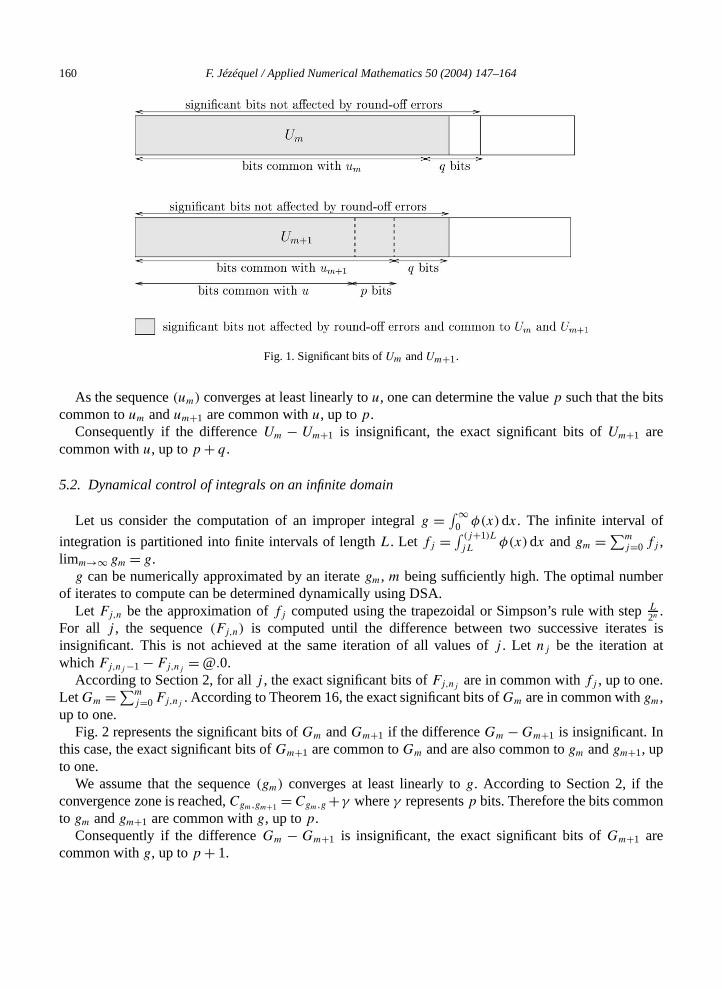
160 F. Jézéquel / Applied Numerical Mathematics 50 (2004) 147–164
er
es ist
n
Fig. 1. Significant bits ofUm andUm+1.
As the sequence(um) converges at least linearly tou, one can determine the valuep such that the bitscommon toum andum+1 are common withu, up top.
Consequently if the differenceUm − Um+1 is insignificant, the exact significant bits ofUm+1 arecommon withu, up top + q.
5.2. Dynamical control of integrals on an infinite domain
Let us consider the computation of an improper integralg = ∫ ∞0 φ(x)dx. The infinite interval of
integration is partitioned into finite intervals of lengthL. Let fj = ∫ (j+1)L
jLφ(x)dx andgm = ∑m
j=0 fj ,limm→∞ gm = g.
g can be numerically approximated by an iterategm, m being sufficiently high. The optimal numbof iterates to compute can be determined dynamically using DSA.
Let Fj,n be the approximation offj computed using the trapezoidal or Simpson’s rule with stepL2n .
For all j , the sequence(Fj,n) is computed until the difference between two successive iteratinsignificant. This is not achieved at the same iteration of all values ofj . Let nj be the iteration awhich Fj,nj −1 − Fj,nj
= @.0.According to Section 2, for allj , the exact significant bits ofFj,nj
are in common withfj , up to one.Let Gm = ∑m
j=0 Fj,nj. According to Theorem 16, the exact significant bits ofGm are in common withgm,
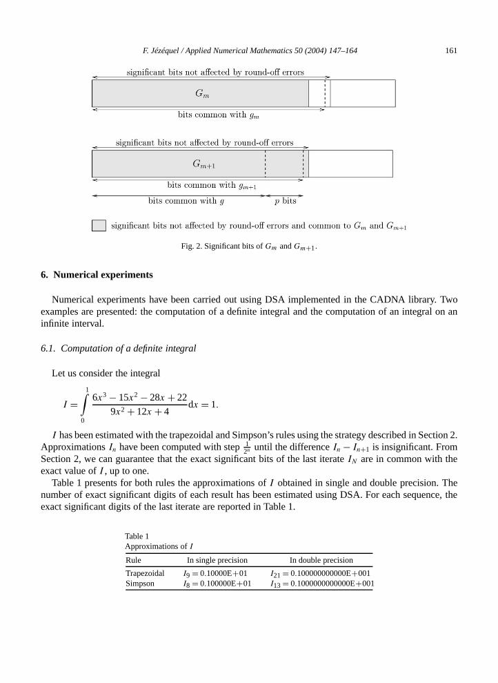
up to one.Fig. 2 represents the significant bits ofGm andGm+1 if the differenceGm − Gm+1 is insignificant. In
this case, the exact significant bits ofGm+1 are common toGm and are also common togm andgm+1, upto one.
We assume that the sequence(gm) converges at least linearly tog. According to Section 2, if theconvergence zone is reached,Cgm,gm+1 = Cgm,g +γ whereγ representsp bits. Therefore the bits commoto gm andgm+1 are common withg, up top.
Consequently if the differenceGm − Gm+1 is insignificant, the exact significant bits ofGm+1 arecommon withg, up top + 1.
F. Jézéquel / Applied Numerical Mathematics 50 (2004) 147–164 161
oal on an
ection 2.
hence, the
Fig. 2. Significant bits ofGm andGm+1.
6. Numerical experiments
Numerical experiments have been carried out using DSA implemented in the CADNA library. Twexamples are presented: the computation of a definite integral and the computation of an integrinfinite interval.
6.1. Computation of a definite integral
Let us consider the integral
I =1∫
0
6x3 − 15x2 − 28x + 22
9x2 + 12x + 4dx = 1.
I has been estimated with the trapezoidal and Simpson’s rules using the strategy described in SApproximationsIn have been computed with step12n until the differenceIn − In+1 is insignificant. FromSection 2, we can guarantee that the exact significant bits of the last iterateIN are in common with theexact value ofI , up to one.
Table 1 presents for both rules the approximations ofI obtained in single and double precision. Tnumber of exact significant digits of each result has been estimated using DSA. For each sequeexact significant digits of the last iterate are reported in Table 1.
Table 1Approximations ofI
Rule In single precision In double precision
Trapezoidal I9 = 0.10000E+01 I21 = 0.100000000000E+001Simpson I8 = 0.100000E+01 I13 = 0.1000000000000E+001
162 F. Jézéquel / Applied Numerical Mathematics 50 (2004) 147–164
We can notice that the exact significant digits of each approximation obtained are in common withI .The number of iterations requested for the stopping criterion to be satisfied depends of course on the
tions aregencee
ns as in
ce
n to two
therroren) isre not
e,
precision chosen, but also on the quadrature method used. Whatever the precision is, less iteraperformed with Simpson’s rule than with the trapezoidal rule. This is due to the different converspeeds of the computed sequences. Indeed the approximation ofI is of order 2 with the trapezoidal ruland of order 4 with Simpson’s rule. For each rule, the error on the last iterate|IN − I | is insignificant.Because of round-off error propagation, the computer cannot distinguishIN from I .
6.2. Computation of an improper integral
Let us consider the improper integral
g =∞∫
0
e−ax dx = 1
a,
wherea > 0.g has been estimated using the strategy described in Section 5.2. Using the same notatio
Section 5.2, letgm = ∑mj=0 fj , wherefj = ∫ (j+1)L
jLe−ax dx. The approximations of the integralsfj are
computed with Simpson’s rule using DSA. For everyj , a sequence is computed until the differenbetween two successive iterates is insignificant.
As gm − g = ∫ ∞(m+1)L
e−ax dx = αm+1
a, whereα = e−aL, the sequence(gm) converges linearly tog.
Therefore Theorem 5 can apply: if the convergence zone is reached, the significant bits commosuccessive iterates are also common tog, up to log2(
11−α
).Let Gm be the approximation ofgm computed using DSA. The sequence(Gm) is computed until
the difference between two successive iterates is insignificant. We denote byM the iteration at whichGM−1 − GM = @.0. According to Section 5.2, the exact significant bits ofGM are in common withg,up to log2(
11−α
) + 1. Therefore the exact significant decimal digits ofGM are in common withg up toδ,whereδ = log10(
21−α
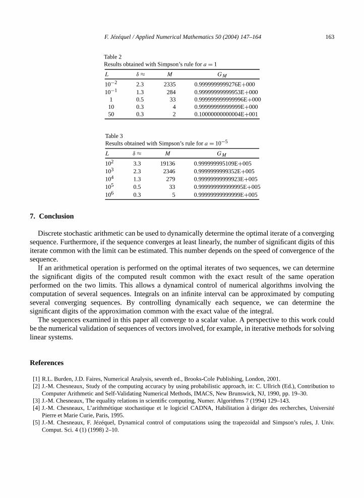
).Table 2 presents fora = 1 and different values ofL the approximationsGM obtained in double
precision. The number of exact significant digits ofGM not in common withg is approximated byδ.As the lengthL increases, the numberM of integralsfj to be approximated decreases. Onlyexact significant digits ofGM are reported: the other significant digits are affected by round-off epropagation. We notice that the number of exact significant digits obtained (from thirteen to fiftesatisfying for computations carried out in double precision. The exact significant digits which ain common with the exact valueg = 1 can easily be identified. For example, ifL = 10−1, among thefourteen exact significant digits ofGM , the two last digits are not in common withg. We notice that, forevery approximationGM reported in Table 2, its exact significant digits are in common withg up to�δ .
Table 3 presents fora = 10−5 and different values ofL the exact significant digits of thapproximationsGM obtained in double precision. As in Table 2, we notice that if the lengthL increasesthe numberM of integralsfj to be approximated decreases. For each approximationGM obtained, wecan easily identify its exact significant digits which are in common with the exact valueg = 105. As inTable 2, we notice that the exact significant digits ofGM are in common withg up to�δ .
F. Jézéquel / Applied Numerical Mathematics 50 (2004) 147–164 163
Table 2Results obtained with Simpson’s rule fora = 1
vergingts of thisce of the
termineeration
theputing
ine the
rk couldsolving
to
iversité
niv.
L δ ≈ M GM
10−2 2.3 2335 0.9999999999276E+00010−1 1.3 284 0.99999999999953E+000
1 0.5 33 0.999999999999996E+00010 0.3 4 0.99999999999999E+00050 0.3 2 0.10000000000004E+001
Table 3Results obtained with Simpson’s rule fora = 10−5
L δ ≈ M GM
102 3.3 19136 0.999999995109E+005103 2.3 2346 0.9999999999352E+005104 1.3 279 0.99999999999923E+005105 0.5 33 0.999999999999995E+005106 0.3 5 0.99999999999999E+005
7. Conclusion
Discrete stochastic arithmetic can be used to dynamically determine the optimal iterate of a consequence. Furthermore, if the sequence converges at least linearly, the number of significant digiiterate common with the limit can be estimated. This number depends on the speed of convergensequence.
If an arithmetical operation is performed on the optimal iterates of two sequences, we can dethe significant digits of the computed result common with the exact result of the same opperformed on the two limits. This allows a dynamical control of numerical algorithms involvingcomputation of several sequences. Integrals on an infinite interval can be approximated by comseveral converging sequences. By controlling dynamically each sequence, we can determsignificant digits of the approximation common with the exact value of the integral.
The sequences examined in this paper all converge to a scalar value. A perspective to this wobe the numerical validation of sequences of vectors involved, for example, in iterative methods forlinear systems.
References
[1] R.L. Burden, J.D. Faires, Numerical Analysis, seventh ed., Brooks-Cole Publishing, London, 2001.[2] J.-M. Chesneaux, Study of the computing accuracy by using probabilistic approach, in: C. Ullrich (Ed.), Contribution
Computer Arithmetic and Self-Validating Numerical Methods, IMACS, New Brunswick, NJ, 1990, pp. 19–30.[3] J.-M. Chesneaux, The equality relations in scientific computing, Numer. Algorithms 7 (1994) 129–143.[4] J.-M. Chesneaux, L’arithmétique stochastique et le logiciel CADNA, Habilitation à diriger des recherches, Un
Pierre et Marie Curie, Paris, 1995.[5] J.-M. Chesneaux, F. Jézéquel, Dynamical control of computations using the trapezoidal and Simpson’s rules, J. U
Comput. Sci. 4 (1) (1998) 2–10.
164 F. Jézéquel / Applied Numerical Mathematics 50 (2004) 147–164
[6] J.-M. Chesneaux, J. Vignes, Sur la robustesse de la méthode CESTAC, C. R. Acad. Sci. Paris Sér. I Math. 307 (1988)855–860.
5 (1992)
ss, New
glewood
974.
1.in: Proc.
[7] J.-M. Chesneaux, J. Vignes, Les fondements de l’arithmétique stochastique, C. R. Acad. Sci. Paris Sér. I Math. 311435–1440.
[8] M.K. Jain, R.K. Jain, S.R.K. Iyengar, Numerical Methods for Scientific and Engineering Computation, Halsted PreYork, 1985.
[9] J.H. Mathews, Numerical Methods for Mathematics, Science and Engineering, second ed., Prentice-Hall, EnCliffs, NJ, 1992.
[10] J. Vignes, M. La Porte, Error analysis in computing, in: Information Processing ’74, North-Holland, Amsterdam, 1[11] J. Vignes, Zéro mathématique et zéro informatique, C. R. Acad. Sci. Paris Sér. I Math. 303 (1986) 997–1000;
also: Vie Sci. 4 (1) (1987) 1–13.[12] J. Vignes, Estimation de la précision des résultats de logiciels numériques, Vie Sci. 7 (2) (1990) 93–145.[13] J. Vignes, A stochastic arithmetic for reliable scientific computation, Math. Comput. Simulation 35 (1993) 233–26[14] J. Vignes, A stochastic approach to the analysis of round-off error propagation. A survey of the CESTAC method,
2nd Real Numbers and Computers Conference, Marseille, France, 1996, pp. 233–251.