DYNAMIC INTERACTION BETWEEN HEAVY VEHICLES AND SPEED BUMPS

Piotr Szurgott

Military University of Technology 2 Gen. Sylwestra Kaliskiego Street

00-908 Warsaw, Poland E-mail: pszurgott@wat.edu.pl

Leslaw Kwasniewski Warsaw University of Technology

Al. Armii Ludowej 16 00-637 Warsaw, Poland

E-mail: l.kwasniewski@il.pw.edu.pl

Jerry W. Wekezer FAMU-FSU College of Engineering

2525 Pottsdamer Street Tallahassee, FL 32310

E-mail: wekezer@eng.fsu.edu KEYWORDS Computer simulation, heavy vehicles, speed bumps, LS-DYNA. ABSTRACT

The paper presents finite element (FE) model development and experimental validation for a truck tractor with a three axle single drop lowboy trailer. The main objective of this research activity was to create a simplified, three dimensional virtual FE model, applicable for computer simulation of dynamic interaction between a vehicle and a bridge or road structure. Such model should provide a reliable approximation of dynamic loadings exerted by the wheels to the bridge or pavement structure for a wide range of total weights and speeds considered. To meet this requirement the FE model should have correct mass distribution and properly represented stiffness characteristics of the suspension system. As explicit laboratory testing of the suspension system requires its disassembling and is very expensive, an indirect method was applied to find the stiffness and damping characteristics of the suspension. The study reported in this paper consists of experimental and numerical parts. During the experimental tests the vehicle was driven across the speed bumps at different speeds. The relative displacement and acceleration histories were recorded for several points located on the vehicle axles and the frame. In addition, a speed bump was scanned on site using a laser scanner. The experimental data was subsequently used for the development and calibration of the spring and damping characteristics for suspension systems of the FE model. The numerical part was based on non-linear, explicit, dynamic, finite element (FE) analysis using the LS-DYNA computer code. INTRODUCTION

One of the important issues for maintenance and design engineers is the magnitude of actual dynamic loads exerted by heavy vehicles on bridges and roads. Experimental, analytical, and numerical studies were conducted to estimate the actual values of impact factors which represent dynamic overloading as compared with static loads (Kwasniewski et al. 2006). A need for consideration of a wide variety of heavy vehicle

configurations suggests a selection of computer methods as the most effective and flexible. Heavy vehicles are usually considered in such analyses as simplified systems of rigid masses connected through linear or nonlinear springs and dampers (Fafard and Bennur 1997, Green and Cebon 1997, Huang et al. 1998, and Piombo et al. 2000). Besides the correct mass distribution, a model of a heavy vehicle should have an appropriate representation of the actual suspension system. Characteristics of the vehicle suspension can be determined through experimental compression tests conducted either on an isolated suspension system or indirectly through field experiments conducted on an entire vehicle. The purpose of each test is to determine stiffness and damping characteristics of the suspension. The first method is expensive as it requires removal of the suspension from the existing vehicle or a purchase of a new one. Displacement of the piston of the shock absorber is measured and recorded as a function of the load applied. This relationship is non-linear and is usually simplified by piecewise linear functions. Idealized, perfectly fixed boundary conditions in direct suspension testing do not account for sometimes worn out and partially loose connections between the suspension and the vehicle. In addition, testing of a new suspension system will often result in different suspension characteristics as compared with those in actual and used vehicles. In the indirect method the tests are conducted on an entire vehicle which moves along predefined road surface profiles with different loads and at different speeds (Lehtonen 2005, Letherwood and Gunter 2001, and Valášek et al. 1998). Typical data acquisition from such tests usually includes time histories of accelerations and relative displacements between selected points. Filtered experimental output is analyzed and used for validation of analytical or numerical models. The first approximation of the suspension characteristics can also be obtained for some of the technical solutions using simplified formula developed by the automotive industry. Such formula allow for calculation of linear stiffness of leaf spring suspension based on dimensions of leaves and their number. The disadvantage of the indirect method is the difficulty in measuring dynamic interaction forces between suspension components or between wheels and the road surface.

Proceedings 23rd European Conference on Modelling andSimulation ©ECMS Javier Otamendi, Andrzej Bargiela,José Luis Montes, Luis Miguel Doncel Pedrera (Editors)ISBN: 978-0-9553018-8-9 / ISBN: 978-0-9553018-9-6 (CD)

Correct representation of wheel and tire models is another important issue in modeling of heavy vehicle dynamic behavior. In very simple models the wheels are represented by lumped masses with time dependent, moving, concentrated reactions. However, modern computational techniques allow modeling the wheels as rotating, pneumatic, three dimensional objects interacting with the road surface through a well defined contact algorithm. The burden of complexity of such an approach is addressed by the FE code used for the simulation. This type of approach is easier and more reliable as it requires fewer simplifying assumptions. The main objective of this research activity is to develop a simplified FE model of a heavy vehicle applicable for transient analysis of dynamic interaction between a vehicle and a bridge or a road surface. Such a model provides a reliable approximation of dynamic loading exerted by the wheels on the bridge or pavement. It is expected that the procedure developed here will be easily adaptable for a wide range of heavy vehicles with different gross vehicle weights (GVW), suspension characteristics, and speeds. A popular heavy vehicle, a single unit tractor-trailer with a three axle single-drop lowboy, was chosen as representative for this study. The paper describes its FE model development and experimental validation through on-site experimental tests. A numerical analysis presented here is based on non-linear, explicit, dynamic, finite element (FE) computational mechanics using the LS-DYNA computer code. During the experimental tests the heavy vehicle was driven across a speed bump at different speeds. Relative displacement and acceleration histories were collected for several points located on vehicle’s axles and frame. In addition, an actual, typical speed bump was scanned using a laser scanner and a resulting FE model of the speed bump was developed. The experimental data was subsequently used for the development and validation of the spring and damping characteristics for all suspension systems of the FE model.

FINITE ELEMENT MODELS

FE models of the Truck Tractor and Single-Drop Lowboy Trailer

The truck tractor, with a three axle single-drop lowboy trailer as shown in Figure 1a, was selected for this study. A complete FE model of the tractor and the trailer consists of over 25,000 finite elements. It is presented in Figure 1b with an additional cargo of the total mass of 39,000 kg. It is planned that this fully loaded vehicle will be used in further experimental tests of dynamic interaction between a bridge and a moving vehicle. The HyperMesh Software from Altair was used as a pre-processor for modeling. In-situ measurements and data available from the manufacturers’ websites were used for developing the FE model. The selected truck is one of the most popular in the U.S. The wheelbase for the truck is 4.73 meters long and may vary between 3.68 and 6.10 meters. The tandem axle spacing in the rear suspension remains the same for each wheelbase. Therefore, future, simple modifications of the wheelbase in the FE model are possible and they can be easily implemented by adding or removing FE elements from the longitudinal truck frame. Development of the suspension system and identification of its major components are presented in Figure 2. Each suspension consists of the rotating horizontal axles located along corresponding non-rotating axles which are connected to the frame through vertical cylindrical joints. All axles are modeled using rigid beam elements. The rotation of a rotating axle is implemented by using a constraint option, referred to as a revolute joint in LS-DYNA (LS-DYNA 2007). The vertical movement of an axle set is achieved by using the cylindrical joints and the special purpose massless discrete elements which simulate springs and shock absorbers, as presented in Figure 2.

4.07m 1.32m 8.69m 1.24m 1.24m

b)

a)

Figure 1: Selected Truck Tractor and Single-Drop Lowboy Trailer (a) and Their FE Model (b)

Rotating PartNon-Rotating Part

Moving Part

Cylindrical JointRevolute Joint

Non-Rotating Axle Rotating Axle Vertica l Cylindrical Joint

Drum

Attached to Frame

a)

b)

Damper Viscous

Frame

Spring Elastic

Discrete Elements

Vertica tl Cylindrical Join

Non-Rotating Axle

Figure 2: FE Model of the Front Suspension System. Schemes of Constrained Joints (a) and Discrete

Elements (b) used to Connect Rigid Components

The entire FE model of the front suspension includes the steering axle, two leaf springs, and two shock absorbers. Other components such as the frame hangers, bushings, height control system, upper shock brackets and axle attachment hardware were lumped together as a sprung mass connected with the bodywork. Their mass was added to the equivalent parts connected with the frame through the Vertical Cylindrical Joint (see Figure 2). Tandem axles with air springs are modeled in the rear suspension system in the similar way as observed in the actual truck. Each axle suspension includes air springs, shock absorbers, a cross channel, main support members, an ultra rod, torque rods, an axle, and frame brackets. The total mass of these components was lumped together into an equivalent part in the FE model. In the suspension system of the actual trailer, two leaf springs per axle are used in an underslung configuration with a 127 mm round axle. The total weight of each suspension system was estimated based on the available data. In the FE model, the mass of each axle was distributed between rotating and non-rotating axles represented by 2D beam elements. The actual truck has 22.5"×8.25" aluminum wheels, whereas the trailer is equipped with steel 2 hand-hole wheels 22.5"×7.50" in size. Two types of shell elements were used for modeling – 3-node elements for the discs and 4-node elements for the rims, see Figure 3. Both units have tubeless tires. A simple pressure volume airbag model was used for the FE pneumatic models of the tires. The values of pressure inside the airbags were set up according to data provided by the tire manufacturer and can be easily changed in the FE model. The FE model of the tire consists of the sidewalls and the tread parts. Each of these components includes two coincident layers of 4-node shell elements. The first layer represents rubber-like material with average properties for rubber, whereas the second layer (representing the cord) uses a material model for fabrics, with stiffness for tension only.

The thicknesses of the shell elements used for wheels and tires was based on the data available from manufacturer websites; however some of them were modified in order to obtain masses similar to the actual wheels. The FE model of the complete wheel including disc, rim, sidewalls, and tread, is presented in Figure 3.

Rubber Tread Rubber Sidewalls

Fabric Sidewalls

Rim

Disc

Fabric Tread

Figure 3: FE Model of Wheel (a) and its Components – Sidewalls and Tread include Two Layers of Elements

for Rubber and Fabric Materials

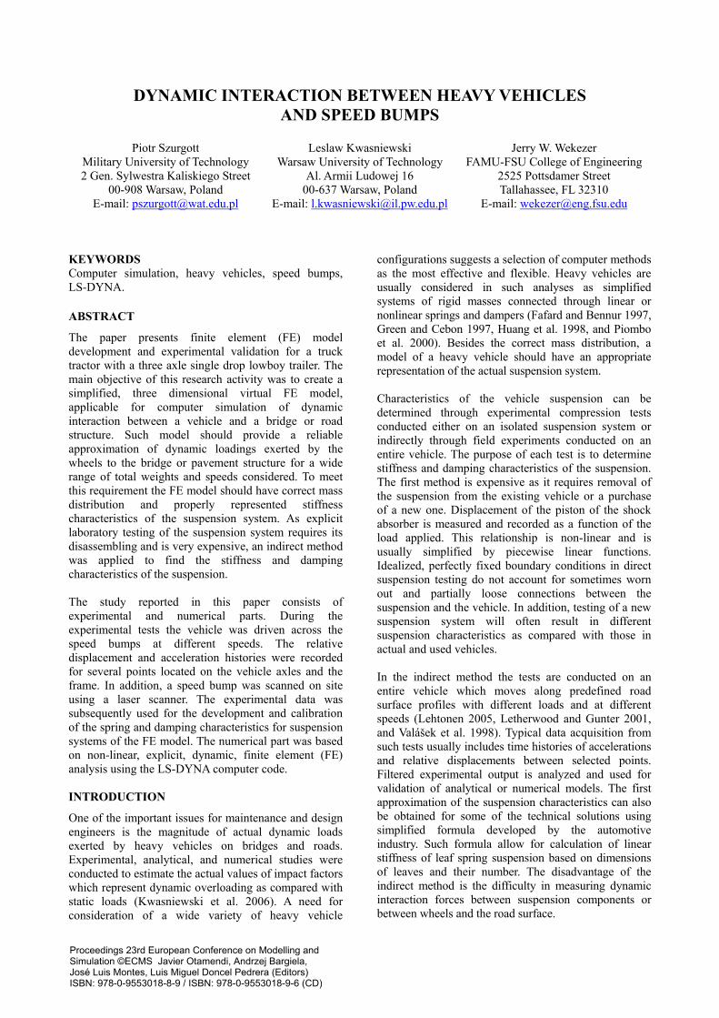
The major objective of this project was to determine the effect of the speed bumps on the dynamic behavior of the heavy vehicle. Therefore, the complete FE model of the tractor and trailer was simplified, as detailed modeling of each component was not necessary to achieve the project goal. The simplifications included primarily the bodywork where the driver cab, hood, fuel tanks, and engine were modeled as rigid bodies. Moreover, the FE models of the drive and steering systems were also simplified and they do not include transmission, transmission shafts and a few other components. These simplifications not only helped in reducing the size of the FE model and the CPU time needed but they also made all the calculations more stable and reliable. The selected single drop lowboy trailer was constructed using standard U.S. structural steel profiles including: C-channels, S-flanges and wide flanges (Engineers Edge 2008). 4-node shell elements were used for the FE modeling. Additional load in the form of crane counterweights was modeled as a rigid body using solid elements. The revolute joints were also used in the "fifth" wheel connection, as shown in Figure 4. They allow for the relative movement of the trailer in the vertical plane. For all of the performed analysis the FE model was restricted to the straight direction and any movements of the trailer in the horizontal plane were not allowed. Hence, the fifth wheel and the skid plate of the trailer were rigidly connected. The suspension systems and the tires received much attention in the modeling process as clearly having a distinct influence on the interaction between vehicle and the road surface. Finding all the necessary data for suspension development took a significant amount of

Fifth Wheel

Constrained Joint Revolute

Frame

Skid Plate

Coincident Nodes

b)

a)

Fifth Wheel

Figure 4: FE Model of the Fifth Wheel (a). Connection between Fifth Wheel and the Skid Plate (b)

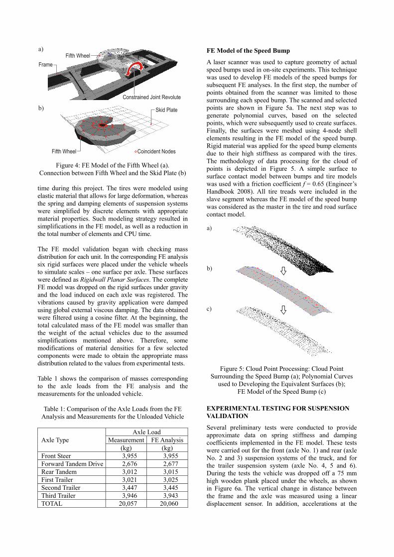
time during this project. The tires were modeled using elastic material that allows for large deformation, whereas the spring and damping elements of suspension systems were simplified by discrete elements with appropriate material properties. Such modeling strategy resulted in simplifications in the FE model, as well as a reduction in the total number of elements and CPU time. The FE model validation began with checking mass distribution for each unit. In the corresponding FE analysis six rigid surfaces were placed under the vehicle wheels to simulate scales – one surface per axle. These surfaces were defined as Rigidwall Planar Surfaces. The complete FE model was dropped on the rigid surfaces under gravity and the load induced on each axle was registered. The vibrations caused by gravity application were damped using global external viscous damping. The data obtained were filtered using a cosine filter. At the beginning, the total calculated mass of the FE model was smaller than the weight of the actual vehicles due to the assumed simplifications mentioned above. Therefore, some modifications of material densities for a few selected components were made to obtain the appropriate mass distribution related to the values from experimental tests. Table 1 shows the comparison of masses corresponding to the axle loads from the FE analysis and the measurements for the unloaded vehicle.

Table 1: Comparison of the Axle Loads from the FE Analysis and Measurements for the Unloaded Vehicle

Axle Load Axle Type Measurement FE Analysis (kg) (kg) Front Steer 3,955 3,955 Forward Tandem Drive 2,676 2,677 Rear Tandem 3,012 3,015 First Trailer 3,021 3,025 Second Trailer 3,447 3,445 Third Trailer 3,946 3,943 TOTAL 20,057 20,060

FE Model of the Speed Bump

A laser scanner was used to capture geometry of actual speed bumps used in on-site experiments. This technique was used to develop FE models of the speed bumps for subsequent FE analyses. In the first step, the number of points obtained from the scanner was limited to those surrounding each speed bump. The scanned and selected points are shown in Figure 5a. The next step was to generate polynomial curves, based on the selected points, which were subsequently used to create surfaces. Finally, the surfaces were meshed using 4-node shell elements resulting in the FE model of the speed bump. Rigid material was applied for the speed bump elements due to their high stiffness as compared with the tires. The methodology of data processing for the cloud of points is depicted in Figure 5. A simple surface to surface contact model between bumps and tire models was used with a friction coefficient f = 0.65 (Engineer’s Handbook 2008). All tire treads were included in the slave segment whereas the FE model of the speed bump was considered as the master in the tire and road surface contact model.

a)

b)

c)

Figure 5: Cloud Point Processing: Cloud Point Surrounding the Speed Bump (a); Polynomial Curves

used to Developing the Equivalent Surfaces (b); FE Model of the Speed Bump (c)

EXPERIMENTAL TESTING FOR SUSPENSION VALIDATION

Several preliminary tests were conducted to provide approximate data on spring stiffness and damping coefficients implemented in the FE model. These tests were carried out for the front (axle No. 1) and rear (axle No. 2 and 3) suspension systems of the truck, and for the trailer suspension system (axle No. 4, 5 and 6). During the tests the vehicle was dropped off a 75 mm high wooden plank placed under the wheels, as shown in Figure 6a. The vertical change in distance between the frame and the axle was measured using a linear displacement sensor. In addition, accelerations at the

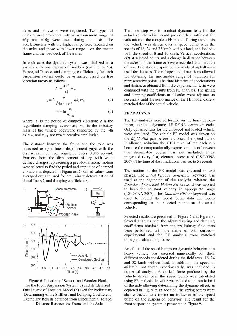
axles and bodywork were registered. Two types of uniaxial accelerometers with a measurement range of ±5g and ±10g were used during the tests. The accelerometers with the higher range were mounted on the axles and those with lower range – on the tractor frame and the load deck of the trailer. In each case the dynamic system was idealized as a system with one degree of freedom (see Figure 6b). Hence, stiffness ki and damping coefficient ci for each suspension system could be estimated based on free vibration theory as follows:

bid

i mk2

24τπ

= (1)

biii mkc224

2δπ

δ+

= (2)

)1(

ln+

=i

i

uuδ (3)

where: τd is the period of damped vibration; δ is the logarithmic damping decrement; mbi is the tributary mass of the vehicle bodywork supported by the i-th axle; ui and u(i+1) are two successive amplitudes. The distance between the frame and the axle was measured using a linear displacement gage with the displacement changes registered every 0.005 second. Extracts from the displacement history with well-defined changes representing a pseudo-harmonic motion were selected to find the period and amplitude of damped vibration, as depicted in Figure 6c. Obtained values were averaged out and used for preliminary determination of the stiffness ki and damping coefficient ci.

mb1

c1k1Position Sensor

Wooden Plank

Accelerometersa) b)

c)

Time (s)0.0 0.5 1.0 1.5 2.0 2.5 3.0 3.5 4.0 4.5 5.0

Dista

nce (

mm)

367

369

371

373

375

377

τd3

Axle No. 1 Considered Section

τd4τd2τd1

u2u1 u3 u4

Figure 6: Location of Sensors and Wooden Plank for the Front Suspension System (a) and its Idealized

One Degree of Freedom Model (b) used for Preliminary Determining of the Stiffness and Damping Coefficient. Exemplary Results obtained from Experimental Test (c)

– Distance Between the Frame and the Axle

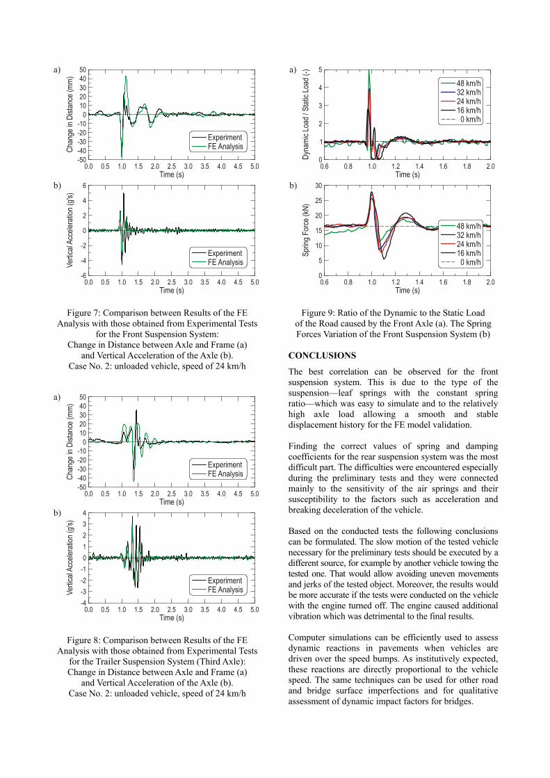
The next step was to conduct dynamic tests for the actual vehicle which could provide data sufficient for validation of the complete FE model. During these tests the vehicle was driven over a speed bump with the speeds of 16, 24 and 32 km/h without load, and loaded - with the speed of 8 and 16 km/h. Vertical accelerations a(t) at selected points and a change in distance between the axles and the frame u(t) were recorded as a function of time. Two standard speed bumps made of asphalt were used for the tests. Their shapes and dimensions allowed for obtaining the measurable range of vibration for representative points. The time histories of accelerations and distances obtained from the experimental tests were compared with the results from FE analyses. The spring and damping coefficients at all axles were adjusted as necessary until the performance of the FE model closely matched that of the actual vehicle. FE ANALYSIS

The FE analyses were performed on the basis of non-linear, explicit, dynamic LS-DYNA computer code. Only dynamic tests for the unloaded and loaded vehicle were simulated. The vehicle FE model was driven on the Rigid Wall part before it crossed the speed bump. It allowed reducing the CPU time of the each run because the computationally expensive contact between two deformable bodies was not included. Fully integrated (very fast) elements were used (LS-DYNA 2007). The time of the simulations was set to 5 seconds. The motion of the FE model was executed in two phases. The Initial Velocity Generation keyword was used at the beginning of the analysis, whereas the Boundary Prescribed Motion Set keyword was applied to keep the constant velocity in appropriate range (LS-DYNA 2007). The Database History keyword was used to record the nodal point data for nodes corresponding to the selected points on the actual vehicle. Selected results are presented in Figure 7 and Figure 8. Several analyses with the adjusted spring and damping coefficients obtained from the preliminary field tests were performed until the shape of both curves—experimental and the FE analysis—were matched through a calibration process. An effect of the speed bumps on dynamic behavior of a heavy vehicle was assessed numerically for three different speeds considered during the field tests: 16, 24 and 32 km/h without load. In addition, the speed of 48 km/h, not tested experimentally, was included in numerical analysis. A vertical force produced by the vehicle driven over the speed bump was calculated using FE analysis. Its value was related to the static load of the axle allowing determining the dynamic effect, as depicted in Figure 9. In addition, the spring forces were also extracted to estimate an influence of the speed bump on the suspension behavior. The result for the front suspension system is presented in Figure 9.

Time (s)0.0 0.5 1.0 1.5 2.0 2.5 3.0 3.5 4.0 4.5 5.0

-50

-20-10

0

20

5040

-30

a)

-40Chan

ge in

Dist

ance

(mm)

ExperimentFE Analysis

10

30

Time (s)0.0 0.5 1.0 1.5 2.0 2.5 3.0 3.5 4.0 4.5 5.0

Vertic

al Ac

celer

ation

(gs)'

b) 6

-4

-2

0

2

4

-6

ExperimentFE Analysis

Figure 7: Comparison between Results of the FE Analysis with those obtained from Experimental Tests

for the Front Suspension System: Change in Distance between Axle and Frame (a)

and Vertical Acceleration of the Axle (b). Case No. 2: unloaded vehicle, speed of 24 km/h

Time (s)0.0 0.5 1.0 1.5 2.0 2.5 3.0 3.5 4.0 4.5 5.0

-50

-100

1020

50

30

- 02- 03

a)

Chan

ge in

Dist

ance

(mm) 40

-40

ExperimentFE Analysis

Time (s)0.0 0.5 1.0 1.5 2.0 2.5 3.0 3.5 4.0 4.5 5.0

b)

Vertic

al Ac

celer

ation

(gs)'

ExperimentFE Analysis

4

-3-2

0

23

-4

-1

1

Figure 8: Comparison between Results of the FE Analysis with those obtained from Experimental Tests

for the Trailer Suspension System (Third Axle): Change in Distance between Axle and Frame (a)

and Vertical Acceleration of the Axle (b). Case No. 2: unloaded vehicle, speed of 24 km/h

a)

Time (s)0.6 0.8 1.0 1.2 1.4 1.8 2.0

Dyna

mic L

oad /

Stat

ic Lo

ad (-

)

0

1

2

3

4

5

24 km/h32 km/h48 km/h

16 km/h0 km/h

1.6

b)

Time (s)0.6 0.8 1.0 1.2 1.4 1.8 2.01.6

Sprin

g For

ce (

N)k

0

5

10

15

20

30

25

24 km/h32 km/h48 km/h

16 km/h0 km/h

Figure 9: Ratio of the Dynamic to the Static Load of the Road caused by the Front Axle (a). The Spring Forces Variation of the Front Suspension System (b)

CONCLUSIONS

The best correlation can be observed for the front suspension system. This is due to the type of the suspension—leaf springs with the constant spring ratio—which was easy to simulate and to the relatively high axle load allowing a smooth and stable displacement history for the FE model validation. Finding the correct values of spring and damping coefficients for the rear suspension system was the most difficult part. The difficulties were encountered especially during the preliminary tests and they were connected mainly to the sensitivity of the air springs and their susceptibility to the factors such as acceleration and breaking deceleration of the vehicle. Based on the conducted tests the following conclusions can be formulated. The slow motion of the tested vehicle necessary for the preliminary tests should be executed by a different source, for example by another vehicle towing the tested one. That would allow avoiding uneven movements and jerks of the tested object. Moreover, the results would be more accurate if the tests were conducted on the vehicle with the engine turned off. The engine caused additional vibration which was detrimental to the final results. Computer simulations can be efficiently used to assess dynamic reactions in pavements when vehicles are driven over the speed bumps. As institutively expected, these reactions are directly proportional to the vehicle speed. The same techniques can be used for other road and bridge surface imperfections and for qualitative assessment of dynamic impact factors for bridges.

ACKNOWLEDGEMENT

The study reported in this paper was supported by a grant from the Florida Department of Transportation (FDOT) titled: “Investigation of Impact Factors for Permit Vehicles”, FDOT contract No. BD 543. The experimental testing of the vehicle suspension was carried out by a research team from the FDOT Structures Lab including: Stephen Eudy, William Potter and Paul Tighe. Opinions and views expressed in this paper are those of the authors and not necessarily those of the sponsoring Agency. The authors would like to express their appreciation for this generous financial and experimental support. REFERENCES Engineer's Edge. Accessed July 30, 2008.

www.engineersedge.com/structural_shapes_menu.shtml. Engineer’s Handbook. Accessed July 30, 2008.

www.engineershandbook.com/Tables/frictioncoefficients.htm.

Fafard, M., and M. Bennur. 1997. “A General Multi-Axle Vehicle Model to Study the Bridge Vehicle Interaction.” Engineering Computations, Vol. 14, No. 5, pp. 491–508.

Green, M. F., and D. Cebon. 1997. “Dynamic Interaction Between Heavy Vehicles and Bridges.” Computers & Structures, Vol. 62, No. 2, pp. 253–264.

Huang D., T.-L. Wang, M. Shahawy. 1998. “Vibration of Horizontally Curved Box Girder Bridges Due to Vehicles.” Computers & Structures, Vol. 68, No. 5, pp. 513–528.

Kwasniewski, L., J. W. Wekezer, G. Roufa, H. Li, J. Ducher, and J. Malachowski. 2006. „Experimental Evaluation of Dynamic Effects for a Selected Highway Bridge”, ASCE Journal of Performance of Constructed Facilities, Vol. 20, No. 3, pp. 1–8.

Kwasniewski, L., H Li, J. W. Wekezer, and J. Malachowski. 2006. „Finite Element Analysis of Vehicle–Bridge Interaction.” Finite Elements in Analysis and Design, Vol. 42, Issue 11, pp. 950–959.

Lehtonen, T. J. 2005. “Validation of an Agricultural Tractor MBS Model.” International Journal of Heavy Vehicle System, Vol. 12, No. 1, pp. 16–27.

Letherwood, M. D., and D. D. Gunter. 2001. “Ground Vehicle Modeling and Simulation of Military Vehicles Using High Performance Computing.” Parallel Computing, No. 27, pp. 109–140.

LS-DYNA Theory Manual, 2007. Livermore Software Technology Corporation.

Piombo, B. A. D., A. Fasana, S. Marchesiello, and M. Ruzzene. 2000. “Modeling and Identification of the Dynamic Response of Supported Bridge.” Mechanical Systems and Signal Processing, Vol. 14 No, 1, pp. 75–89.

Valášek, M., V. Stejskal, Z. Šika, O. Vaculin, J. Kovanda. 1998. “Dynamic Model of Truck for Suspension Control.” Vehicle System Dynamics, 28 pp. 496–505, Swets & Zeitlinger.

AUTHOR BIOGRAPHIES

PIOTR SZURGOTT is a doctoral student at the Military University of Technology in Warsaw. He earned his MS degree in Mechanics and Machinery Design from Warsaw University of Technology in 2002. He worked on this project as a Research Assistant at the Crashworthiness and Impact Analysis Laboratory (CIAL), FAMU-FSU College of Engineering in Tallahassee in 2007-08. He uses nonlinear, explicit, dynamic finite element methods as his primary tools in his computer modeling and simulation studies. LESLAW KWASNIEWSKI works as an Assistant Professor at the Civil Engineering Department at Warsaw University of Technology (WUT) since 1998. He received all his degrees, including PhD in Civil Engineering in 1997, from WUT. He was awarded a Dekaban Fellowship from the University of Michigan in 1999. He has also collaborated with the CIAL at FAMU-FSU College of Engineering in Tallahassee, FL for over three years. His research interests include: theoretical and experimental applied structural mechanics, applied finite element analysis, engineering finite element modeling, programming, and computer simulations. JERRY WEKEZER is a Distinguished University Professor at the joint FAMU-FSU College of Engineering. He received his degrees from Gdansk Technical University, Poland. His academic career includes a Visiting Professorship at the University of Southern California, a head of the Civil Engineering Department at the University of Alaska Anchorage, and the chairman of the Department of Civil and Environmental Engineering at FAMU-FSU College of Engineering in Tallahassee. He is a funding director of the Crashworthiness and Impact Analysis Laboratory which was established at FAMU-FSU College of Engineering in 1995. He is a licensed Professional Engineer in the states of Alaska and Florida.