University of WarsawFaculty of Mathematics, Informatics and Mechanics

Jakub Łącki

Dynamic Graph Algorithmsfor Connectivity Problems

PhD dissertation

Supervisor

dr hab. Piotr Sankowski prof. UW

Institute of InformaticsUniversity of Warsaw

January 2015

Author’s declaration:aware of legal responsibility I hereby declare that I have written this disser-tation myself and all the contents of the dissertation have been obtained bylegal means.

January 22, 2015 . . . . . . . . . . . . . . . . . . . . . . . . . . . . . .date Jakub Łącki

Supervisor’s declaration:the dissertation is ready to be reviewed

January 22, 2015 . . . . . . . . . . . . . . . . . . . . . . . . . . . . . .date dr hab. Piotr Sankowski prof. UW

AbstractIn this thesis we present several new algorithms for dynamic graph problems.The common theme of the problems we consider is connectivity. In particular,we study the maintenance of connected components in a dynamic graph, andthe Steiner tree problem over a dynamic set of terminals.

First, we present an algorithm for decremental connectivity in planargraphs. It processes any sequence of edge deletions intermixed with a set ofconnectivity queries. Each connectivity query asks whether two given verticesbelong to the same connected component. The running time of this algorithmis optimal, that is, it handles any sequence of updates in linear time, andanswers queries in constant time. This improves over the best previouslyknown algorithm, whose total update time is O(n log n).

Then, we study the dynamic Steiner tree problem. In this problem, givena weighted graph G on a vertex set V and a dynamic set S ⊆ V of termi-nals, subject to insertions and deletions, the goal is to maintain a constant-approximate Steiner tree spanning S in G. For general graphs and everyinteger k ­ 2, we show an (8k − 4)-approximate algorithm, which pro-cesses updates in O(kn1/k log4 n) amortized expected time. In the case ofplanar graphs we show a different solution, whose amortized update time isO(ε−1 log6 n) and the approximation ratio is 4 + ε.

Finally, we study graph connectivity in a semi-offline model. We con-sider a problem, in which the input is a sequence of graphs G1, . . . , Gt, suchthat Gi+1 is obtained from Gi by adding or removing a single edge. In thebeginning, this sequence is given to the algorithm for preprocessing. Afterthat, the algorithm should efficiently answer queries of one of two kinds. Aforall(a, b, u, w) query, where 1 ¬ a ¬ b ¬ t and u, w are vertices, askswhether u and w are connected with a path in each of Ga, Gb, . . . , Gb. Sim-ilarly, an exists(a, b, u, w) query asks if the given vertices are connected inany of Ga, Gb, . . . , Gb. For forall queries, we show an algorithm that afterpreprocessing in O(t log t(log n+ log log t)) expected time answers queries inO(log n log log t) time. In the case of exists queries, the preprocessing timeis O(m+ nt) and the query time is constant.

Key words: dynamic graph algorithms, dynamic connectivity, decrementalconnectivity, Steiner treeAMS Classification: 05C85 Graph algorithms, 68P05 Data structures, 68Q25Analysis of algorithms and problem complexity, 68W40 Analysis of algo-rithms

3

StreszczenieW niniejszej pracy przedstawiamy nowe algorytmy dla dynamicznych pro-blemów grafowych. Wszystkie omawiane problemy dotyczą zagadnienia spój-ności. W szczególności zajmujemy się utrzymywaniem spójnych składowychw zmieniającym się grafie oraz utrzymywaniem drzewa Steinera rozpinają-cego zmieniający się zbiór terminali.

Po pierwsze pokazujemy algorytm dla dekrementalnej spójności w grafachplanarnych. Algorytm ten przetwarza ciąg operacji składający się z usunięćkrawędzi oraz zapytań o spójność. Każde zapytanie sprawdza, czy dwa po-dane wierzchołki należą do tej samej spójnej składowej. Czas działania tegoalgorytmu jest optymalny: przetwarza on dowolny ciąg aktualizacji w czasieliniowym i odpowiada na zapytania w czasie stałym. Poprawia to wcześniej-szy algorytm, którego łączny czas aktualizacji to O(n log n).

Następnie prezentujemy algorytm, który dla ważonego grafu G na zbio-rze wierzchołków V i dla zmieniającego się zbioru terminali S ⊆ V (wierz-chołki są do niego dodawane i z niego usuwane) utrzymuje stałą aproksymacjędrzewa Steinera rozpinającego zbiór S w G. Dla grafów dowolnych i każdegok ­ 2 pokazujemy algorytm (8k − 4)-aproksymacyjny, który przetwarza ak-tualizacje w oczekiwanym czasie zamortyzowanym O(kn1/k log4 n). W przy-padku grafów planarnych pokazujemy szybszy algorytm o zamortyzowanymczasie aktualizacji O(ε−1 log6 n) i współczynniku aproksymacji 4 + ε.

Ponadto badamy spójność grafów w modelu częściowo offline. Rozwa-żamy problem, w którym wejściem jest ciąg grafów G1, . . . , Gt, taki że Gi+1otrzymuje się z Gi przez dodanie lub usunięcie jednej krawędzi. Algorytmpoznaje ten ciąg na początku swego działania i może wykonać preprocessing.Następnie powinien efektywnie odpowiadać na nadchodzące zapytania jed-nego z dwóch rodzajów. Zapytanie forall(a, b, u, w), gdzie 1 ¬ a ¬ b ¬ t, au, w są wierzchołkami, sprawdza, czy u i w są połączone ścieżką w każdym zgrafów Ga, Gb, . . . , Gb. Podobnie zapytanie exists(a, b, u, w) sprawdza, czypodane wierzchołki są połączone w którymkolwiek z grafów Ga, Gb, . . . , Gb.Dla zapytań forall pokazujemy algorytm, który po preprocessingu w ocze-kiwanym czasie O(t log t(log n + log log t)) odpowiada na zapytania w cza-sie O(log n log log t). W przypadku zapytań exists czas preprocessingu toO(m+ nt), zaś czas zapytań jest stały.Słowa kluczowe: dynamiczne algorytmy grafowe, dynamiczna spójność, de-krementalna spójność, drzewo SteineraKlasyfikacja tematyczna AMS: 05C85 Graph algorithms, 68P05 Data struc-tures, 68Q25 Analysis of algorithms and problem complexity, 68W40 Analysisof algorithms

5

Judytce

Contents

1 Introduction 101.1 Dynamic Connectivity . . . . . . . . . . . . . . . . . . . . . . 13

1.1.1 General Graphs . . . . . . . . . . . . . . . . . . . . . . 131.1.2 Planar Graphs and Trees . . . . . . . . . . . . . . . . . 141.1.3 Dynamic MST . . . . . . . . . . . . . . . . . . . . . . 141.1.4 Our Results . . . . . . . . . . . . . . . . . . . . . . . . 15

1.2 Dynamic Steiner Tree . . . . . . . . . . . . . . . . . . . . . . . 181.2.1 Our Results . . . . . . . . . . . . . . . . . . . . . . . . 19

1.3 Organization of This Thesis . . . . . . . . . . . . . . . . . . . 201.4 Articles Comprising This Thesis . . . . . . . . . . . . . . . . . 201.5 Acknowledgments . . . . . . . . . . . . . . . . . . . . . . . . . 20

2 Preliminaries 222.1 Graphs . . . . . . . . . . . . . . . . . . . . . . . . . . . . . . . 22

2.1.1 Basic Definitions . . . . . . . . . . . . . . . . . . . . . 222.1.2 Connectivity . . . . . . . . . . . . . . . . . . . . . . . . 232.1.3 Weighted Graphs . . . . . . . . . . . . . . . . . . . . . 232.1.4 Trees . . . . . . . . . . . . . . . . . . . . . . . . . . . . 242.1.5 Planar Graphs . . . . . . . . . . . . . . . . . . . . . . 25

2.2 Segment Trees . . . . . . . . . . . . . . . . . . . . . . . . . . . 262.3 Algorithms . . . . . . . . . . . . . . . . . . . . . . . . . . . . . 29

2.3.1 Approximation Algorithms . . . . . . . . . . . . . . . . 292.3.2 Dynamic Graph Algorithms . . . . . . . . . . . . . . . 302.3.3 Connectivity . . . . . . . . . . . . . . . . . . . . . . . . 302.3.4 String Hashing . . . . . . . . . . . . . . . . . . . . . . 32

2.4 Other Remarks . . . . . . . . . . . . . . . . . . . . . . . . . . 33

3 Decremental Connectivity in Planar Graphs 343.1 Preliminaries . . . . . . . . . . . . . . . . . . . . . . . . . . . 343.2 O(n log n) Time Algorithm . . . . . . . . . . . . . . . . . . . . 353.3 O(n log log n) Time Algorithm . . . . . . . . . . . . . . . . . . 37

8

3.4 O(n log log log n) Time Algorithm . . . . . . . . . . . . . . . . 423.5 O(n) Time Algorithm . . . . . . . . . . . . . . . . . . . . . . . 45

4 Dynamic Steiner Tree 474.1 Bipartite Emulators . . . . . . . . . . . . . . . . . . . . . . . . 474.2 Constructing Bipartite Emulators . . . . . . . . . . . . . . . . 53

4.2.1 General Graphs . . . . . . . . . . . . . . . . . . . . . . 534.2.2 Planar Graphs . . . . . . . . . . . . . . . . . . . . . . 55

4.3 Related Results . . . . . . . . . . . . . . . . . . . . . . . . . . 59

5 Connectivity in Graph Timelines 605.1 Connectivity History Tree . . . . . . . . . . . . . . . . . . . . 615.2 exists Queries . . . . . . . . . . . . . . . . . . . . . . . . . . 64

5.2.1 Answering Queries . . . . . . . . . . . . . . . . . . . . 675.3 forall Queries . . . . . . . . . . . . . . . . . . . . . . . . . . 70

5.3.1 Answering Queries . . . . . . . . . . . . . . . . . . . . 765.3.2 Deterministic Algorithm . . . . . . . . . . . . . . . . . 77

5.4 Subsequent Results . . . . . . . . . . . . . . . . . . . . . . . . 78

6 Open Problems 79

9

Chapter 1

Introduction

What makes us think that an algorithm is efficient? In the theoretical ap-proach, we consider an algorithm efficient if the number of instructions itexecutes is linear in the size of its input data. This is justified by the factthat usually the algorithm has to read the entire input, or at least a big frac-tion of it. In fact, once we show that a linear time algorithm has to access aconstant fraction of its input data, we may infer that it is optimal.

At the same time, the theoretical optimality of an algorithm may notmean much in real life applications. If we implement a linear time algorithmand run it on data, whose size is measured in terabytes, it may take long tocomplete. While the running time of a single run may be reasonable, if thealgorithm is used repeatedly, our requirements for its running time may bemuch stricter.

However, it is a common scenario that if the data is being processedrepeatedly, between two consecutive computations it only changes slightly.This fact can be exploited to obtain faster algorithms, which, instead ofprocessing the data from scratch after each change, would only process thechanges that are made. Such algorithms are called dynamic and are the maintopic of this thesis.

We focus on dynamic graph algorithms, that is dynamic algorithms thatcan be used to process graphs. A graph algorithm is dynamic if it main-tains information about a graph subject to its modifications. Typically themodifications alter the set of vertices or edges in the graph. The sequence ofmodifications, henceforth called updates, is intermixed with a set of queries.There are various dynamic graph problems, which differ in the allowed typesof queries. For example, the queries may ask about the existence of a pathbetween two given vertices or the weight of the minimum spanning tree ofthe graph. The algorithm should utilize the maintained information to an-swer each query faster than in the time needed to recompute the solution

10

from scratch.There are three kinds of dynamic graph problems, which differ in the types

of updates that can happen. Let us focus on the problems, where the updatesalter the set of edges. In an incremental problem, edges may only be added,whereas in a decremental one, edges can only be deleted. A fully dynamicproblem is more general than the previous two, as both edge insertions anddeletions can take place.

The central problem in the area of dynamic graph algorithm is the dy-namic connectivity problem. In this problem, we are given a graph subjectto edge insertions and deletions, and our goal is to answer queries aboutthe existence of a path connecting two given vertices. Since connectivity is afundamental graph property, the study of dynamic connectivity is importantboth from theoretical and practical points of view.

The dynamic connectivity problem is also a benchmark of the knowntechniques for tackling dynamic graph problems. While it has a simple for-mulation and has received much attention, the first algorithm with polylog-arithmic update time was given in 1995 [20], and it has taken over 15 moreyears to develop the first solution with polylogarithmic worst-case updatetime [26]. However, many questions regarding dynamic connectivity have notbeen answered yet. The running time of the best algorithm of fully dynamicconnectivity is still higher than the lower bound. Similarly, for decrementalconnectivity in general graphs, no lower bound is known.

Only in few special cases we know that the existing solutions are optimal.In particular, there exists an incremental connectivity algorithm [40], whoserunning time matches an existing lower bound [16]. In the case of trees thereexists a decremental connectivity algorithm that processes all updates inlinear time, and answers each query in constant time [3]. Also, for planegraphs1 there exists a fully dynamic algorithm with amortized update timeof O(log n), which matches the lower bound.

In this thesis we finally settle the connectivity problem in one moresetting. We show a decremental connectivity algorithm for planar graphs,which processes updates in linear total time and answers queries in constanttime. This improves over an existing algorithm, whose total update time isO(n log n) and matches the time bound of decremental connectivity in trees.

Moreover, we introduce and solve a new dynamic problem that deals withconnectivity in a semi-offline model. We develop algorithms that process agraph timeline, that is a sequence of graphs G1, . . . , Gt, such that Gi+1 isobtained from Gi by adding or removing a single edge. In this model, an

1A graph is plane if it is planar, and its embedding remains fixed in the course of theoperations.

11

algorithm may preprocess the entire timeline at the beginning, and after thatit should answer queries arriving in online fashion. We consider timelines ofundirected graphs and two types of queries.

An exists(u,w, a, b) query, where u and w are vertices and 1 ¬ a ¬ b ¬ t,asks whether vertices u and w are connected in any of Ga, Ga+1, . . . , Gb. Onthe other hand, a forall(u,w, a, b) query asks whether vertices u and w areconnected in each of Ga, Ga+1, . . . , Gb.

This thesis also deals with another dynamic graph problem, namely dy-namic Steiner tree. Let G = (V,E, dG) be a weighted graph and S ⊆ V bea set of terminals. The Steiner tree spanning S in G is a minimum-weightsubgraph of G, in which every pair of vertices of S is connected. In the dy-namic Steiner tree problem, the set S is dynamic, that is, its elements areinserted and deleted. The goal is to maintain a constant-approximate Steinertree spanning S in G.

The dynamic variant of the Steiner tree problem was introduced by Imaseand Waxman [25] in 1991, and while it has been studied since then, nosolution with sublinear update time has been given. The existing algorithmsfor dynamic Steiner tree focus on minimizing the number of changes to thetree, or use a heuristic approach to minimize the running time.

We show the first solution for dynamic Steiner tree with sublinear updatetime. For any k ­ 2 it processes updates in O(kn1/k log4 n) expected amor-tized algorithm, and maintains a (8k−4)-approximate Steiner tree. Moreover,for planar graphs we show a (4 + ε)-approximate algorithm, which processeseach update in O(ε−1 log6 n) amortized time.

The Steiner tree problem is closely related to the minimum spanning tree(MST) problem. First, the MST problem is a special case of the Steiner treeproblem, where every vertex of the graph is a terminal. More importantly,there also exists a reverse relation. We may use an algorithm for computingMST to compute an approximate Steiner tree. This is achieved by buildinga complete graph on the set of terminals, where the edge weight of an edgeuw is the distance between u and w in the original graph. It is well-knownthat the MST of this complete graph corresponds to a 2-approximate Steinertree.

The Steiner tree problem and MST are also related in the dynamic setting.The 2-approximate algorithm can be made dynamic, using an algorithm fordynamic MST, which gives an algorithm for dynamic Steiner tree with anupdate time of O(n). The sublinear time algorithm for dynamic Steiner tree,that we give in this thesis, also uses dynamic MST as a subroutine.

In the following part of this chapter, we describe our results and theirrelation to the previously obtained algorithm in the area.

12

Update time Query time Type Authors

O(log n(log log n)3) O(log n/ log log n) Monte Carlo, amrt. Thorup [42]

O(log2 n/ log log n) O(log n/ log log n) deterministic, amrt. Wulff-Nilsen [47]

O(log5 n) O(log n/ log log n) Monte Carlo, w-c Kapron et al. [26]

O(√

n) O(1) deterministic, w-c Eppstein et al. [12]

Figure 1.1: Algorithms for fully dynamic connectivity in general graphs. W-cstands for worst-case, whereas amrt. means amortized.

1.1 Dynamic ConnectivityIn the dynamic connectivity problem, given a graph subject to edge updates,the goal is to answer queries about the existence of a path connecting twovertices. We first review the previously obtained algorithms for this problem,both for general graphs and some restricted graph classes. Then, we showour results in this area and present their relation to the existing results.

1.1.1 General GraphsFully Dynamic Connectivity

There has been a long line of research considering the fully dynamic connec-tivity in general graphs [15, 12, 20, 23, 42, 26, 47]. The study of this problemwas initiated by Frederickson [15] about 30 years ago, but the first polylog-arithmic time algorithm has been given over 10 years later [20]. The firstalgorithm with polylogarithmic worst-case update time was shown in 2013by Kapron and King [26], but the algorithm is randomized. A deterministicalgorithm with polylogarithmic worst-case update time is not known, and ob-taining such an algorithm is a major open problem. The best currently knownalgorithms for fully dynamic connectivity are summarized in Figure 1.1.

Concerning lower bounds, Henzinger and Fredman [21] obtained a lowerbound of Ω(log n/ log log n) in the RAM model. This was improved by De-maine and Patrascu [38] to a lower bound of Ω(log n) in cell-probe model.Both these lower bounds hold also for plane graphs.

Incremental Connectivity

Incremental graph connectivity can be solved using an algorithm for theunion-find problem. It follows from the result of Tarjan [40] that a sequence

13

of t edge insertions and t queries can be handled in O(tα(t)) time, whereα(t) is the extremely slowly growing inverse Ackermann function. A matchinglower bound (Ω(α(n)) time per operation) has been shown by Fredman andSaks [16] in the cell probe model.

Decremental Connectivity

For the decremental variant, Thorup [41] has shown a randomized algo-rithm, which processes any sequence of edge deletions in O(m log(n2/m) +n(log n)3(log log n)2) time and answers queries in constant time. Here, m isthe initial number of edges in the graph. If m = Θ(n2), the update time isO(m), whereas for m = Ω(n(log n log log n)2) it is O(m log n).

1.1.2 Planar Graphs and TreesThe situation is much simpler in the case of planar graphs. Eppstein et.al [14] gave a fully dynamic algorithm, which handles updates and queriesin O(log n) amortized time, but it works only for plane graphs, that is, itrequires that the graph embedding remains fixed. For the general case (i.e.,when the embedding may change) Eppstein et. al [13] gave an algorithm withO(log2 n) worst-case update time and O(log n) query time.

In planar graphs, the best known solution for the incremental connectiv-ity problem is the union-find algorithm. On the other hand, for the decre-mental problem nothing better than a direct application of the fully dy-namic algorithm is known. This is different from both general graphs andtrees, where the decremental connectivity problems have better solutionsthan what could be achieved by a simple application of their fully dynamiccounterparts. In the case of general graphs, the best total update time isO(m log n) [41] (except for very sparse graphs, including planar graphs), com-pared to O(m log n(log log n)3) time for the fully dynamic variant. For trees,only O(n) time is necessary to perform all updates in the decremental sce-nario [3], while in the fully dynamic case one can use dynamic trees that mayhandle each update in O(log n) worst-case time.

1.1.3 Dynamic MSTIn the dynamic MST problem, the input is a weighted undirected graph G =(V,E, dG), subject to edge insertions and removals. The goal is to maintainthe weight of the MST of G, as the set of edges is modified. The only efficiencyparameter is the time needed to process a single update.

14

Update time Type AuthorsO(√m) worst-case Frederickson [15]

O(√n) worst-case Eppstein [12]

O( 3√n log n) amortized Henzinger, King [22]

O(log4 n) amortized Holm et al. [23]

Figure 1.2: The history of algorithms for dynamic MST. All the algorithmslisted here are deterministic.

This problem is closely related with the dynamic connectivity problem,and some techniques are common for both these problems. While the algo-rithms for dynamic connectivity maintain a spanning tree of a graph, thealgorithms for dynamic MST maintain a minimum spanning tree. In somecases, new techniques for dynamic connectivity also implied better algorithmsfor dynamic MST [15, 23].

The algorithms for dynamic MST are listed in Figure 1.2. The fastestknown algorithm processes updates in O(log4 n) amortized time [23]. Con-trary to dynamic connectivity, no algorithm with polylogarithmic worst-caseupdate time is known. In fact even finding an algorithm with o(

√n) worst-

case update time is an open problem [26]. In addition to that, even thoughthe best dynamic algorithms for connectivity are randomized, this is not thecase for dynamic MST.

Dynamic MST has also been considered in the offline model. In this model,the input is a sequence of weighted graphs G1, . . . , Gt, such that Gi+1 isobtained from Gi by changing the weight of a single edge. Eppstein [11] hasshown an algorithm, which computes the weight of the MST of every Gi inO(t log n) total time. We use the techniques developed by Eppstein in ouralgorithms for answering exists and forall queries.

1.1.4 Our ResultsDecremental Connectivity in Planar Graphs

We show an algorithm for the decremental connectivity problem in planargraphs, which processes any sequence of edge deletions in O(n) time andanswers queries in constant time. This improves over the previous bound ofO(n log n), which can be obtained by applying the fully dynamic algorithmby Eppstein [14], and matches the running time of decremental connectivity

15

on trees [3].In fact, we present a O(n) time reduction from the decremental connec-

tivity problem to a collection of incremental problems in graphs of total sizeO(n). These incremental problems have a specific structure: the set of allowedunion operations forms a planar graph and is given in advance. As shown byGustedt [19], such a problem can be solved in linear time.

Our result shows that in terms of total update time, the decrementalconnectivity problem in planar graphs is definitely not harder than the in-cremental one. Though, it should be noted that the union-find algorithmcan process any sequence of k query or update operations in O(kα(n)) time,while in our algorithm we are only able to bound the time to process anysequence of edge deletions.

Moreover, since fully dynamic connectivity has a lower bound of Ω(log n)(even in plane graphs) shown by Demaine and Patrascu [38], our resultsimply that in planar graphs decremental connectivity is strictly easier thanthe fully dynamic one. We suspect that the same holds for general graphs,and we conjecture that it is possible to break the Ω(log n) bound for a singleoperation of a decremental connectivity algorithm, or the Ω(m log n) boundfor processing a sequence of m edge deletions.

Our algorithm, unlike the majority of algorithms for maintaining con-nectivity, does not maintain the spanning tree of the current graph. As aresult, it does not have to search for a replacement edge when an edge fromthe spanning tree is deleted. Our approach is based on a novel and verysimple approach for detecting bridges, which alone gives O(n log n) total up-date time. We use the fact that a deletion of edge uw in the graph causessome connected component to split if both sides of uw belong to the sameface. This condition can in turn be verified by solving an incremental con-nectivity problem in the dual graph. When we detect a deletion that splits aconnected component, we start two parallel DFS searches from u and w toidentify the smaller of the two new components. Once the first search fin-ishes, the other one is stopped. A simple argument shows that this algorithmruns in O(n log n) time.

We then show that the DFS searches can be speeded up using an r-division, that is a decomposition of a planar graph into subgraphs of sizeat most r = log2 n. This gives an algorithm running in O(n log log n) time.For further illustration of this idea we show how to apply it twice in orderto obtain an O(n log log log n) time algorithm. Then, we observe that theO(n log log log n) time algorithm reduces the problem of maintaining connec-tivity in the input graph to maintaining connectivity in a number of graphsof size at most O(log2 log n). The number of all graphs on so few vertices isso small that we can simply precompute the answers for all of them and use

16

these precomputed answers to obtain the linear-time algorithm. The prepro-cessing of all graphs of bounded size is again an idea that, to the best ofour knowledge, has never been previously used for designing dynamic graphalgorithms.

Connectivity in Graph Timelines

We also study graph connectivity in a semi-offline model. We develop algo-rithms that process a graph timeline, that is a sequence of graphs G1, . . . , Gt,such that Gi+1 is obtained from Gi by adding or removing a single edge. Inthis model, an algorithm may preprocess the entire timeline at the begin-ning, and after that it should answer queries arriving in online fashion. Weconsider timelines of undirected graphs and two types of queries.

An exists(u,w, a, b) query, where u and w are vertices and 1 ¬ a ¬ b ¬ t,asks whether vertices u and v are connected in any of Ga, Ga+1, . . . , Gb. Weshow an algorithm that after preprocessing in O(m + nt) time may answersuch queries in O(1) time (assuming t = O(nc)). Moreover, it may computeall indices of the graphs, in which u and w are connected, returning themone by one with constant delay.

We also consider forall(u,w, a, b) query, which asks whether verticesu and w are connected in each of Ga, Ga+1, . . . , Gb. For this problem, weshow an algorithm whose expected preprocessing time is O(m+t log t(log n+log log t)) (m denotes the number of edges in G1) and the query time isO(log n log log t). The algorithm is randomized and answers queries correctlywith high probability.

The algorithms for both types of queries are based on a segment tree overthe entire sequence G1, . . . , Gt. We call this tree a connectivity history tree(CHT). Assume that t is a power of 2. Then, the CHT can be computedrecursively as follows. The parameter of the recursion is a fragment of thesequence G1, . . . , Gt, which can be represented as a discrete interval. For aninterval [a, b] (we begin with an interval [1, t]) we consider a graph G[a,b]obtained by keeping only the edges that are present in every graph amongGa, . . . , Gb and compute its connected components. Then, if a < b, we recurseon the first and second halves of the interval [a, b]. We say that every interval,which is at some point the parameter of the recursion, is an elementaryinterval. It is a well-known fact that the number of elementary intervals isO(t) and every interval [a, b], where 1 ¬ a ¬ b ¬ t can be partitioned intoO(log t) elementary intervals.

In the case of exists queries, for every elementary interval [a, b] we pre-compute the answer to every possible exists(u,w, a, b) query. We make someobservations that allow us to precompute the answers in only O(m+nt) time

17

(instead of O(n2t)). Using this information, we could answer an arbitraryquery by partitioning the query interval into O(log t) elementary intervals.However, we show a more involved query algorithm, which answers queriesin constant time. Our ideas for speeding up the preprocessing phase followthe techniques used by Eppstein [11].

The algorithm for answering forall queries is more involved. For everyvertex v we define a sequence Cv = c1

v, . . . , ctv, where ci

v is the identifier of theconnected component of v inGi. In order to answer a query forall(u,w, a, b),we compute and compare the hashes of sequences ca

u, . . . , cbu and ca

w, . . . , cbw.

The computation of hashes requires an initial preprocessing. We use theconnectivity history tree to compute connectivity information about everygraph G1, . . . , Gt in near linear time. Using this information we precomputehashes of some prefixes of Cv, which are then used to efficiently compute thedesired hashes. It should be noted that our results in this area have beenrecently speeded up and simplified by Karczmarz [27].

1.2 Dynamic Steiner TreeThe next dynamic graph problem that we consider is the dynamic Steiner treeproblem. The static variant of the Steiner tree problem is NP-complete, and,unless P = NP , does not admit a PTAS, even in complete graphs with edgeweights restricted to 1 and 2. In general graphs, only a 1.39-approximatealgorithm is known [8]. On the other hand, the problem admits a PTASin geometric graphs, i.e., when the edge weights are the Euclidean distancesbetween the points in finite dimensional geometric space [4, 37] and in planargraphs [7]. The PTAS for planar graphs is asymptotically very efficient, i.e.,we can construct an (1 + ε)-approximate Steiner tree in O(n log n) time.

The dynamic Steiner tree problem was first introduced in the pioneer-ing paper by Imase and Waxman [25] and its study was later continuedin [34, 17, 18]. However, all these papers focus on minimizing the numberof changes to the tree that are necessary to maintain a good approximation,and ignore the problem of efficiently finding these changes. The efficiency ofthese online algorithms is measured in terms of the number of replacementsthat are performed after every terminal insertion or deletion. The algorithmsfor dynamic Steiner tree usually represent the Steiner tree as a set of shortestpaths between pairs of vertices, and a replacement is every change made tothis set of paths.

The original algorithm of Imase and Waxman [25] made O(n3/2) replace-ments during the processing of a sequence of n update operations. This wasimproved in the incremental case to O(log n) per terminal insertion by Megow

18

et al. [34]. Later, Gu, Gupta and Kumar [17, 18] have shown that after ev-ery update only O(1) replacements are needed in amortized sense. Moreover,they showed that if terminals are only deleted, it is possible to maintain aconstant approximate Steiner tree making only a single change after everyterminal deletion.

The problem of maintaining the Steiner tree is also an important problemin the network community [9], and while it has been studied for many years,the research resulted only in several heuristic approaches [5, 1, 24, 39] noneof which has been formally proven to have sublinear running time.

1.2.1 Our ResultsWe show the first sublinear time algorithm for the dynamic Steiner treeproblem. For general graphs and any k ­ 2, we give a O(kn1/k log4 n) timealgorithm, which maintains a (8k − 4)-approximate Steiner tree. The timebound is expected and amortized. Moreover, we show a (4 + ε)-approximatealgorithm for planar graphs, which processes updates in O(ε−1 log6 n) amor-tized time.

To the best of our knowledge, previously only a simple O(n) time al-gorithm was known. This algorithm first computes the metric closure G ofthe graph G, and then maintains the MST of G[S] using a polylogarithmicdynamic MSF (minimum spanning forest) algorithm [23]. It is a well-knownfact that this yields a 2-approximate Steiner tree. In order to update G[S] weneed to insert and remove terminals together with their incident edges, whatrequires Θ(n) calls to the dynamic MSF structure. However, such a linearbound is far from being satisfactory, as it does not lead to any improvementin the running time for sparse networks, where m = O(n).2 In such networksafter each update we can actually compute a 2-approximate Steiner tree inO(n log n) time from scratch [35].

Our algorithm for dynamic Steiner tree uses an auxiliary graph calleda bipartite emulator. It is a low-degree bipartite graph, which can be usedto approximate distances in the original graph. Roughly speaking, in ouralgorithm we maintain a subgraph H of the bipartite emulator, which changeswith every change to the set of terminals. We show that the MSF of Happroximates the Steiner tree spanning the set of terminals in the originalgraph. To obtain the algorithm for dynamic Steiner tree, we run dynamicMSF algorithm on the graph H.

We construct different bipartite emulators for general and planar graphs,which results in different running times. While our emulators are constructed

2It is widely observed that most real-world networks are sparse [10].

19

using previously known distance oracles [44, 43], our contribution lies in theintroduction of the concept of bipartite emulators, whose properties make itpossible to solve the dynamic Steiner tree problem in sublinear time usingdynamic MSF algorithm.

1.3 Organization of This ThesisThis thesis is organized as follows. In Chapter 2 we review basic conceptsrelated to graph algorithms, introduce notation and review some existingresults that we use. In the following three chapters we describe our results.Chapter 3 shows the algorithm for decremental connectivity in planar graphs.In Chapter 4 we describe our algorithms for dynamic Steiner tree problem ingeneral and planar graphs. Then, in Chapter 5 we deal with the algorithmsfor processing graph timelines. Finally, in Chapter 6 we list some interestingopen problems related to the problems we consider.

1.4 Articles Comprising This ThesisThe contents of this thesis have been included in the following papers:

• Dynamic Steiner tree and subgraph TSP, joint work with Jakub Oćwie-ja, Marcin Pilipczuk, Piotr Sankowski, and Anna Zych, preliminaryversion available in [31].

• Optimal decremental connectivity in planar graphs, joint work withPiotr Sankowski, to appear at STACS 2015, preliminary version avail-able in [33].

• Reachability in graph timelines, joint work with Piotr Sankowski, pub-lished at ITCS 2013 [32].

This thesis contains only some of the results of the papers listed above.Only the results whose main contributor is the author of this thesis areincluded here.

1.5 AcknowledgmentsI would like to thank my supervisor, Piotr Sankowski, for his motivation,numerous fruitful discussions, and patience with answering lots of my ques-tions. I would also like to thank Krzysztof Diks, who helped me whenever it

20

was needed. I am very grateful to all co-authors of my publications on theo-retical computer science: Krishnendu Chatterjee, Tomasz Idziaszek, TomaszKulczyński, Yahav Nussbaum, Jakub Oćwieja, Marcin Pilipczuk, Jakub Ra-doszewski, Christian Wulff-Nilsen and Anna Zych, as well as my friendsŁukasz Bieniasz-Krzywiec and Dariusz Leniowski. I would like to expressmy gratitude to my great teachers: Krzysztof Benedyczak, who taught meprogramming, and Ryszard Szubartowski, who taught me algorithmics. Fi-nally, I would like to thank my closest relatives, especially my fiancee andmy parents for their endless and ongoing support.

During three years of my studies, my research was supported by GoogleEuropean Doctoral Fellowship in Graph Algorithms, which provided me fi-nancial support and saved tons of paperwork.

21

Chapter 2

Preliminaries

2.1 Graphs

2.1.1 Basic DefinitionsAn undirected graph is a pair G = (V,E), where V is a finite set of verticesand E is a set of edges. Each edge is an unordered pair of elements of V ,that is E ⊆ u,w | u,w ∈ V . A directed graph is also a pair G = (V,E),where V is a finite set of vertices and E is a set of edges. However, edges ofa directed graph are ordered pairs of elements of V . Unless stated otherwise,when referring to a graph we mean an undirected graph. We typically usethe letter n to denote the number of vertices in a graph, and m to denotethe number of edges. Moreover, we use V (G) and E(G) to denote the setsof, respectively, vertices and edges of a graph G.

Let e = u,w be an edge of an undirected graph. We call u and w theendpoints of an edge e. In the following, for simplicity, we use uw to denotean edge, whose endpoints are u and w. We say that e is incident to u andw, u and w are adjacent to e, and u and w are adjacent to each other. Thedegree of a vertex is the number of edges incident to it. The neighborhood ofa vertex v, denoted Γ(v) is the set of vertices adjacent to v.

A walk in a graph G = (V,E) is a sequence of vertices v1, v2, . . . , vk, wherek ­ 1, and for 1 ¬ i < k, vivi+1 is an edge of G. The same definition appliesto directed graphs. The endpoints of a walk v1, v2, . . . , vk are v1 and vk andthe length of this walk is k − 1. A path is a walk v1, v2, . . . , vk, where all vi

are distinct.A subgraph of a graph G = (V,E) is a graph G′ = (V ′, E ′), where V ′ ⊆ V

and E ′ ⊆ E. Note that since G′ is required to be a graph, for every e′ ∈ E ′,both endpoints of e′ belong to V ′. With a slight abuse of notation, if S ⊆ V ,we denote by G \ S a subgraph of G obtained by removing vertices of S and

22

all their incident edges. Similarly, if v ∈ V , we use G \ v to denote G \ v.Let V ′ ⊆ V be a set of vertices. A subgraph of G induced by V ′, denoted

G[V ′] is a subgraph G′ = (V ′, E ′) of G, where E ′ is the set of all edges ofE, whose both endpoints are in V ′. Similarly, for a set E ′ ⊆ E of edges, wedefine G′ = (V ′, E ′) to be an edge-induced subgraph of G, if V ′ is the set ofall endpoints of E ′.

A graph G = (V,E) is a bipartite graph if the set V can be partitionedinto two sets V1, V2, such that V = V1∪V2, V1∩V2 = ∅, and each edge of G hasexactly one endpoint in each of V1 and V2. When describing a bipartite graphwe sometimes write G = (V1 ∪ V2, E) to give the aforementioned partition ofits vertex set. A complete graph is a graph that contains an edge connectingevery pair of its vertices. If G is a complete graph over a set of vertices V ,we write G = (V,

(V2

)). Finally, we say that G = (V,E) is a multigraph if V

is the set of vertices and E is a multiset of pairs of vertices, that is G mayhave multiple edges between a pair of vertices. The definitions that apply tographs can be extended to multigraphs in a natural way.

2.1.2 ConnectivityTwo vertices u, w of a graph G = (V,E) are connected if there is a path inG, whose endpoints are u and w. We say that G is connected, if every twovertices of G are connected. A connected component of G is a subset C ⊆ V ,such that every two vertices of C are connected and C is maximal (withrespect to inclusion).

Proposition 2.1.1. Connected components of a graph G = (V,E) form apartition of V .

Let G = (V,E) be a graph. An edge e ∈ E is a bridge, if (V,E \ e) hasmore connected components than G. A graph G = (V,E) is biconnected if itis connected and for every v ∈ V , G \ v is connected.

A separator of a graph G = (V,E) is a set S ⊆ V , such that G \ Shas more connected components than G. A separator is balanced if the sizeof every connected component of G \ S is at most α|V | for some universalconstant α (in this thesis we can assume α = 3/4).

2.1.3 Weighted GraphsA graph G is weighted if G = (V,E, dG), and dG : E → R is a functionassigning weights to edges of G. Throughout this thesis, we assume that theweights are nonnegative. A subgraph of a weighted graph G = (V,E, dG) is aweighted graph G′ = (V ′, E ′, dG′), such that (V ′, E ′) is a subgraph of (V,E)

23

and dG′ is a restriction of dG to E ′. Other definitions for unweighted graphscan be extended to weighted graphs in a similar manner. On the other hand,the definitions for weighted graphs can be used with unweighted ones. Insuch a case, we assume that the weight of every edge is equal to 1.

Let G′ = (V ′, E ′, dG′) be a subgraph of a weighed graph G = (V,E, dG).We slightly abuse notation and use dG(G′) to denote ∑e′∈E′ dG′(e′). We callthis value the weight of G′. Similarly, for a walk P = v1, v2, . . . , vk in G weuse dG(P ) to denote the weight of this walk equal to ∑k−1

i=1 dG(vivi+1).Let u, w be two vertices of a weighted graph G. The shortest path con-

necting u and w is a minimum weight path whose endpoints are u and w. Ifu and w are connected, the distance between u and w is the weight of theshortest path connecting u and w. Otherwise, the distance between u and wis assumed to be ∞. We denote the distance between u and w by δG(u,w).A metric closure of a weighted graph G = (V,E, dG), denoted G, is a com-plete graph G = (V,

(V2

), dG), where the length of an edge uw is the distance

between u and w in G, that is dG(uw) = δG(u,w).

2.1.4 TreesA graph G = (V,E) is a tree if for every two vertices u,w ∈ V there is aunique path connecting u and w. A graph G = (V,E) is a forest if for everytwo vertices u,w ∈ V there is at most one path connecting u and w.

A vertex v of a tree or forest is called a leaf if its degree is equal to1. A spanning tree of a graph G = (V,E) is any subgraph T = (V,ET ) ofG which is a tree. A spanning forest of a graph G = (V,E) is any sub-graph F = (V,EF ) of G which is a forest and has the same number ofconnected components as G. A minimum spanning tree (MST) of a weightedgraph G = (V,E, dG), denoted MST (G), is a spanning tree of G of minimalweight. Similarly, a minimum spanning forest (MSF) of a weighted graphG = (V,E, dG), is a spanning forest of G of minimal weight. For every setS ⊆ V , we say that a tree T = (V,E) spans S.

Let G = (V,E, dG) be a weighted graph and S ⊆ V be a subset of vertices.A Steiner tree of G, denoted ST (G) is a subgraph T = (VT , ET , dT ) of G,such that S ⊆ VT , every two vertices of S are connected in T and T hasminimal possible weight. We call S the set of terminal vertices or terminals.

A rooted tree is a tree with a distinguished vertex called the root. If v ∈ Vis not a root, we define the parent of v, denoted Parent(v) to be the firstvertex on the unique path from v to the root. If a vertex u is adjacent to avertex w and u is not a parent of w, we say that u is a child of w. If u and ware two vertices of a rooted tree and u lies on the path from w to the root,

24

we say that u is an ancestor of w and w is a descendant of u.A binary tree is a rooted tree, in which every non-leaf vertex has exactly

two children. Moreover, we assume that the children of every vertex v areordered, that is there is a distinguished left child (denoted Left(v)) and aright child (denoted Right(v)). A complete binary tree is a binary tree, inwhich the distance between the root and every leaf is the same. We call thisdistance the height of the tree.

2.1.5 Planar GraphsA plane embedding of a graph G = (V,E) is a mapping of G into R2, whichmaps vertices of G into points and edges of G into simple arcs. Each vertexv is mapped to a distinct point π(v) of a plane. An edge uw is mapped to anarc connecting π(u) and π(w). The arcs corresponding to two distinct edgesdo not intersect except, possibly, at endpoints. A graph is called planar if itadmits a plane embedding.

Consider a plane embedding of a planar graph G = (V,E). The arcs ofthe embedding partition the plane into regions that we call faces. Exactlyone face is unbounded. We call it the outer face. We say that a face f isadjacent to the edges corresponding to the arcs bounding f .

Theorem 2.1.2 (Euler’s formula). Let G = (V,E) be a plane embeddedgraph. Let v be the number of vertices of G, e be the number of edges, f bethe number of faces and c be the number of connected components. Then

v − e+ f = c+ 1.

We say that a planar graph is triangulated if every face is adjacent toexactly three edges.

A dual graph of a planar graph G is a multigraph G∗ obtained by em-bedding a single vertex in every face of G. Let e be an edge of G, which isadjacent to faces f1 and f2. For each such edge, we add to G∗ the dual edgeof e, which connects vertices embedded in f1 and f2.

Proposition 2.1.3. A dual graph of a planar graph is planar.

Note that although we have not defined planar multigraphs (only planargraphs), our definition of planarity can be naturally extended to multigraphs.

A region R is an edge-induced subgraph of G. A boundary vertex of aregion R is a vertex v ∈ V (R) that is adjacent to an edge e 6∈ E(R). Wedenote the set of boundary vertices of a region R by ∂(R). An r-divisionP of G is a partition of G into O(n/r) edge-disjoint regions (which might

25

share vertices), such that each region contains at most r vertices and O(√r)

boundary vertices. The set of boundary vertices of a division P , denoted∂(P) is the union of the sets ∂(R) over all regions R of P . Note that |∂(P)| =O(n/

√r).

Lemma 2.1.4 ([29, 45]). Let G = (V,E) be an n-vertex biconnected trian-gulated planar graph and 1 ¬ r ¬ n. An r-division of G can be constructedin O(n) time.

2.2 Segment TreesThroughout this section we consider discrete intervals, that is intervals ofintegers. The length of such an interval is the number of its elements. Let tbe a power of 2. We define the set of elementary intervals over 1, . . . , t asfollows. First, [1, t] is an elementary interval. Second, if [a, b] is an elemen-tary interval and a < b, then also [a, (a + b − 1)/2] and [(a + b + 1)/2, b]are elementary intervals. For example, the set of elementary intervals over1, . . . , 8 is [1, 8], [1, 4], [5, 8], [1, 2], [3, 4], [5, 6], [7, 8], [1, 1], [2, 2], [3, 3], [4, 4],[5, 5], [6, 6], [7, 7], [8, 8]. Observe that the elementary intervals can be or-ganized into a complete binary tree, in which the root is [1, t], and for anelementary interval [a, b], where a < b, Left([a, b]) = [a, (a + b − 1)/2] andRight([a, b]) = [(a+b+1)/2, b]. This tree is called a segment tree. In the restof this section we implicitly assume that elementary intervals we refer to areover 1, . . . , t and a segment tree is a segment tree over this set of elementaryintervals.

Proposition 2.2.1. The height of the segment tree is O(log t).

Proof. Consider a path that starts in the root and goes to the left child untila leaf is reached. The height of this tree is the length of this path. Each edgeon this path connects an interval with an interval that is half shorter. Sincewe start in [1, t], the path has length O(log t).

Proposition 2.2.2. There are 2t− 1 elementary intervals.

Proof. For i = 0, . . . , log2 t, The segment tree has exactly 2i vertices, whosedistance from the root is i.

From the construction we easily obtain the following.

Proposition 2.2.3. If [a1, b1] and [a2, b2] are elementary intervals, then ei-ther [a1, b1]∩ [a2, b2] = ∅ or one of the intervals is fully contained in the otherone.

26

The set of elementary intervals can be also characterized as follows.

Lemma 2.2.4. Let 1 < a ¬ t and 1 ¬ b ¬ t. There exists an elementaryinterval of length 2i whose right end is b if and only if b is divisible by 2i.Similarly, there exists an interval of length 2i whose left end is a if and onlyif a− 1 is divisible by 2i.

Proof. Let t = 2d. We first show that the set of elementary intervals over1, . . . , t is A = A0 ∪ A1 ∪ . . . Ad, where Ai = [k · 2i + 1, (k + 1) · 2i] | 0 ¬k < 2d−i. We have that Ai has exactly 2d−i elements, each being an intervalof 2i elements. In particular, Ad = [1, t]. Moreover, since the sets Ai aredisjoint, |A| = 2t− 1. By Proposition 2.2.2 there are also 2t− 1 elementaryintervals. Thus the set A and the set of elementary intervals both have size2t− 1. To complete the first part of the proof, it suffices to show that everyelementary interval is contained in A.

In order to do that we show that for i > 0 and any [a, b] ∈ Ai, bothLeft([a, b]) and Right([a, b]) belong to Ai−1. For simplicity, we only showLeft([a, b]) ∈ Ai−1. The second claim is similar.

Since [a, b] ∈ Ai, we have that a = k · 2i + 1 and b = (k + 1) · 2i for0 ¬ k < 2d−i. Recall that Left([a, b]) = [a, (a+ b− 1)/2] = [k · 2i, (2k + 1) ·2i−1] = [2k · 2i−1, (2k+ 1) · 2i−1]. We set k′ = 2k. Since 0 ¬ k < 2d−i, we have0 ¬ k′ < 2d−(i−1). Moreover, Left([a, b]) = [k′ · 2i−1, (k′ + 1) · 2i−1]. Hence,Left([a, b]) ∈ Ai−1, so we conclude that A is exactly the set of elementaryintervals.

Now, fix a value of b ¬ 1. We have that an interval [b − 2i + 1, b] ∈ Ai

if and only if b = (k + 1)2i for some 0 ¬ k < 2d−i. Since 1 ¬ b ¬ t, we canfind a matching k if and only if b is divisible by 2i. Now, consider a > 1. Aninterval [a, a+ 2i− 1] ∈ Ai if and only if a = k · 2i + 1 for some 0 ¬ k < 2d−i.Since 1 < a ¬ t, we can find a matching k if and only if a− 1 is divisible by2i. The lemma follows.

We now show that each interval can be partitioned into O(log t) elemen-tary intervals. Algorithm 1 shows a procedure, which computes such parti-tion.

First, let us note the following property, which follows directly from thepseudocode.

Proposition 2.2.5. Assume we are computing a decomposition of [c, d] intoelementary intervals. In each recursive call Decompose([c′, d′], [a, b]) wehave that [c′, d′] = [c, d] ∩ [a, b].

Lemma 2.2.6. Algorithm 1 produces a decomposition of [c, d] into elemen-tary intervals.

27

Algorithm 11: function Decompose([c, d], [a, b]) . Decompose [c, d] into elementary

intervals, which are sub-intervals of [a, b]Require: [a, b] is an elementary interval and [c, d] ⊆ [a, b]

2: if [c, d] = [a, b] then return [a, b]3: ret := ∅4: if [c, d] ∩ Left([a, b]) 6= ∅ then5: ret := ret ∪Decompose([c, d] ∩ Left([a, b]),Left([a, b]))6: if [c, d] ∩Right([a, b]) 6= ∅ then7: ret := ret ∪Decompose([c, d] ∩Right([a, b]),Right([a, b]))

return ret

Proof. Consider the first parameter [c, d] of Decompose. In every call weeither return a decomposition that contains solely of [c, d] or call Decomposerecursively. The first parameters of the recursive calls form a partition of [c, d].Thus, every element of [c, d] is either returned in a decomposition or passedto a further recursive call. Consequently, the decomposition we return is apartition of [c, d].

Observe that the algorithm terminates, as in every recursive call thelength of the second parameter of Decompose halves. Once we reach aninterval of length 1, that is we call Decompose([c′, d′], [a, a]), we know that[c′, d′] ⊆ [a, a] and [c′, d′] is nonempty (this is a necessary condition to executethe call). Thus, the call terminates returning an interval [a, a]. The lemmafollows.

Lemma 2.2.7. A call to Decompose([c, d], [a, b]), where d = b or c = a,requires O(log(b − a + 1)) time and returns O(log(b − a + 1)) elementaryintervals.

Proof. We assume d = b, the other case is analogous. If Left([a, b])∩ [c, d] 6=∅, then Right([a, b]) ⊆ [c, d]. Thus, both Left([a, b]) and Right([a, b])intersect [c, d], so Decompose([c, d], [a, b]) makes two recursive calls. Thesecond one is Decompose([c, d] ∩ Right([a, b])),Right([a, b])), but sinceRight([a, b]) ⊆ [c, d], the first parameter is simply Right([a, b]). Hence,this call terminates immediately and returns a single interval, so only theother recursive call may trigger further recursive calls.

On the other hand, if Left([a, b])∩ [c, d] = ∅ we only make one recursivecall. In both cases, we spend O(1) time and execute a single recursive call.The second parameter of this recursive call is an interval which is half the sizeof [a, b]. Hence, altogether we spend O(log(b−a+1)) time. Consequently, thelength of the produced decomposition is bounded by O(log(b− a+ 1)).

28

Lemma 2.2.8. Let 1 ¬ a ¬ b ¬ t. The interval [a, b] can be partitioned intoO(log t) elementary intervals over 1, . . . , t in O(log t) time.

Proof. We use Algorithm 1. By Lemma 2.2.6 the algorithm is correct. Itremains to bound the running time. From this, it would follow that thereturned decomposition has length O(log t).

Consider the first recursive call to Decompose which calls Decomposetwice. We call it a branching call. Note that there are at most O(log t) callsbefore a branching call (or O(log t) calls in total, if there is no branchingcall), as in each call the second parameter is an interval that is two timesshorter.

In a branching call we have [c, d] ∩ Left([a, b]) 6= ∅ as well as [c, d] ∩Right([a, b]) 6= ∅. Hence, we may apply Lemma 2.2.7 to both recursive callsthat are made and bound their total running time by O(log(b − a + 1)) =O(log t). The lemma follows.

Note that an interval has multiple possible decompositions into elemen-tary intervals. However, in the following we assume that we use a decompo-sition produced according to Lemma 2.2.8.

Lemma 2.2.9. Let [a, b] be an elementary interval, such that [a, b] ⊆ [c, d].Then the decomposition of [c, d] into elementary intervals contains either[a, b] or one of its ancestors.

Proof. Observe that for every x ∈ [a, b] the intervals containing x are ances-tors of [a, b], [a, b] itself and (a subset of) descendants of [a, b]. It suffices toshow that no descendants of [a, b] belong to the decomposition.

Consider a recursive call Decompose([c′, d′], [a, b]). By Proposition 2.2.5,[c′, d′] = [c, d] ∩ [a, b]). Since [a, b] ⊆ [c, d], we have [c′, d′] = [a, b], so thecall returns immediately. Consequently, Decompose is never called for anydescendant of [a, b] (as a second argument). The lemma follows.

2.3 Algorithms

2.3.1 Approximation AlgorithmsConsider an optimization problem, in which the goal is to compute an object,which satisfies certain properties and has minimal possible weight. An algo-rithm is called α-approximate (for α ­ 1), if it computes a feasible object,whose weight is at most α times the optimal weight.

The following Lemma gives a 2-approximate algorithm for computing theSteiner tree.

29

Lemma 2.3.1. Let G = (V,E, dG) be a weighted graph and S ⊆ V . Then,dG(ST (G)) ¬ MST (G[S]) ¬ 2dG(ST (G)).

Although no polynomial-time algorithm is known for the Steiner treeproblem, both the metric closure and its minimum spanning tree can becomputed in polynomial time.

2.3.2 Dynamic Graph AlgorithmsA dynamic graph algorithm is an algorithm that maintains some informationabout a graph G, which is undergoing modifications. Typically the modifi-cations, in the following called updates, are edge additions or removals. Thesequence of updates is intermixed with a set of queries, e.g., about the ex-istence of a path between two vertices or about the weight of the minimumspanning tree. The algorithm is supposed to answer queries faster than bycomputing the answer from scratch.

In this thesis we work with dynamic graph problems, in which the up-dates change the set of edges in the graph. There are three types of dynamicgraph problems, depending on the allowed modifications. In an incrementalproblem, edges may only be added, whereas in a decremental one, edges canonly be deleted. Finally, a fully dynamic problem allows both edge insertionsand deletions.

In our algorithms we use fully dynamic algorithm that maintains a mini-mum spanning forest of a graph. In the following, we call it a dynamic MSFalgorithm.

Theorem 2.3.2 ([23]). There exists a fully dynamic MSF algorithm, that fora graph on n vertices supports m edge additions and removals in O(m log4 n)total time.

2.3.3 ConnectivityLet G = (V,E) be a graph with n vertices and m edges. It is well knownthat, using depth-first search or breadth-first search algorithms we may findthe connected components of G.

Proposition 2.3.3. Connected components of G can be found in O(n+m)time.

Formally, the algorithm computes for each vertex the unique identifier ofits connected component. Two vertices belong to the same connected com-ponents if and only if their identifiers are equal.

30

Disjoint-Set Data Structure

A disjoint-set data structure (further denoted by DSDS, also called an union-find data structure) maintains a partition of a set of elements into disjointsubsets. In each subset one element is selected as a representative. The datastructure supports two operations. First, given any element x, it can returnthe representative of the subset containing x (this is called the find opera-tion). It can be used to test whether some two elements belong to the sameset of the partition. Moreover, the data structure supports a union opera-tion, which, given two elements x and y, merges the subsets containing x andy. A famous result by Tarjan [40] bounds the running time of a previouslyknown union-find algorithm.

Theorem 2.3.4 ([40]). There exists a disjoint-set data structure that sup-ports any sequence of m operations on an universe of size n in O((n+m)α(n))time, where α is the inverse of Ackerman’s function.

In this thesis however, we need an DSDS, in which the running time ofevery individual operation is bounded. Hence, we use a simple data structurethat we now describe. Each subset in the data structure is represented as arooted tree. The root of the tree is a representative of a subset, and everyother element of a subset maintains a pointer to its parent in the tree. Weassume that the parent pointer of a representative points to itself. Moreover,each representative maintains the size of its subset.

In order to perform the find operation, it suffices to follow the parentpointers, until the representative is reached. To union two subsets we firstfind its representatives x and y. If x = y, nothing has to be done. Otherwise,we compare the sizes of their sets. Assume that the subset of x is not greaterthan the subset of y. In such a case we merge the sets by making y the parentof x.

Let us list some simple properties of the described DSDS.

Proposition 2.3.5. The algorithm takes O(n) time to initialize and performsevery operation in O(log n) worst-case time.

Proposition 2.3.6. The find operation does not change the data structure.Every union operation can change at most one parent pointer in the datastructure. When a change is performed, one representative of the mergedsubsets becomes a parent of the other representative.

The DSDS is closely related to incremental connectivity problem, that isa problem in which we work with a dynamic graph, subject to edge inser-tions. The sequence of insertions is intermixed with queries of the form ‘Are

31

vertices u and w connected?’. It is easy to see that we may use DSDS to solveincremental connectivity problem: a query can be solved by a find operation,whereas an update maps naturally to a union operation. Let G = (V,E) be agraph. We say that a DSDS D is a DSDS of G if D is obtained by performinga union operation for the endpoints of each edge of G.

Proposition 2.3.7. Let G = (V,E) be a graph, and n = |V |. Given a DSDSof a graph G, we can find the connected components of G in O(n) time.

Proof. We view the forest maintained by the DSDS as an undirected graphF . Observe that the connected components of F are the same as the con-nected components of G. Thus, by Proposition 2.3.3, we can find connectedcomponents of F in O(n) time.

2.3.4 String HashingWe use a string hashing scheme based on the fingerprinting technique of Ra-bin and Karp [28]. This scheme can be used to compute hash values (hence-forth called hashes) of strings, that may be used for probabilistic equalitytesting. Throughout this section, let us assume that we work with sequencesof length at most n, that consist of positive integers not greater than M .Let p > max(M,n) be a prime number and B ∈ 0, . . . , p − 1 be chosenuniformly at random. The hash value of a sequence S = s1, . . . , sk is

H(S) =(

k−1∑i=0

Bk−1−isi

)mod p. (2.1)

While the scheme described in [28] chooses p randomly, we modify thescheme slightly, as done, e.g., in [30]. We fix p and then randomly pick B.As shown in [30], this assures that the probability of two distinct sequenceshaving the same hash value is at most n/p. Thus, by choosing a value of pthat is suitably large, yet polynomial in n, distinct sequences have distincthash values with high probability.

We now derive useful properties of this hashing scheme. Note that inorder to use these properties, together with each hash we need to store thelength of the sequence represented by the hash.

Proposition 2.3.8. The hash of a sequence s1, . . . , sk can be computed inO(k) time.

Proof. We use Horner’s rule to evaluate Formula 2.1.

32

Let S1 = a1, . . . , ak and S2 = b1, . . . , bl be two sequences, h1 = H(S1)and h2 = H(S2). We denote by h1 ⊕ h2 the hash of a sequence obtained byappending S2 to S1. Moreover, if S2 be a prefix of S1, we denote by h1 h2the hash of al+1, al+2, . . . ak

Lemma 2.3.9. Let S1 and S2 be two sequences. Given H(S1) and H(S2), wemay compute H(S1)⊕H(S2) in O(1) time. This requires initial preprocessingin O(n) time.

Proof. Let S1 = a1, . . . , ak and S2 = b1, . . . , bl. We have thatH(S1)⊕H(S2) =(H(S1)Bl +H(S2)) mod p. This can be evaluated in O(1) time, if we prepro-cess Bi mod p, for all 1 ¬ i ¬ n.

Lemma 2.3.10. Let S1 be a sequence, and S2 be a prefix of S1. Given H(S1)and H(S2), we may compute H(S1) H(S2) in O(1) time. This requiresinitial preprocessing in O(n) time.

Proof. Let S1 = a1, . . . , ak and S2 = a1, . . . , al for l ¬ k. We have thatH(S1) H(S2) = (H(S1) − Bk−lH(S2)) mod p. This can be evaluated inO(1) time, if we preprocess Bi mod p, for all 1 ¬ i ¬ n.

Lemma 2.3.11. Let S = a1, . . . , ak, where for each 1 ¬ i ¬ k, ai = a1. Then,we may compute H(S) in constant time. This requires initial preprocessingin O(n) time.

Proof. We have that H(S) =(s1∑k−1

i=0 Bi)

mod p. This can be evaluated inconstant time, if we preprocess ∑k−1

i=0 Bi for all 1 ¬ i ¬ n.

2.4 Other RemarksThroughout this thesis we use log x to denote the binary logarithm of x.Moreover, we use log∗ n to denote the iterated logarithm function. We havelog∗ n = 0 for n ¬ 1, and log∗ n = 1 + log∗(log n) for n > 1. We also use thesoft-O notation and write O(f(n)) to denote O(f(n)polylog(n)). Note thatf may have multiple arguments, and the soft-O notation hides factors whichare polylogarithmic in each of them.

We assume word-RAM model with standard instructions. This meansthat the machine word has size w ­ log n. Here, n denotes the size of the inputdata. All basic arithmetic and logical operations (including multiplicationand bit shifts) on integers of at most w bits take unit time.

33

Chapter 3

Decremental Connectivity inPlanar Graphs

In this chapter we show an algorithm for decremental connectivity in planargraphs. The algorithm, at any point, given two vertices of the graph mayanswer whether they belong to the same connected component. The totalrunning time of this algorithm is linear in the size of the graph. By the totalrunning time we denote the total time of handling any sequence of deletionsof edges. Each query is answered in constant time.

In the following part of this chapter we first introduce some definitionsand deal with minor technical issues (in Section 3.1). Then, we present thealgorithm, by introducing our ideas one by one. Each each idea results in afaster algorithm. We describe a simple O(n log n) algorithm in Section 3.2,and then, in Section 3.3, present how to speed it up to O(n log log n) timeusing r-division. Next, in Section 3.4, we show that our idea can be usedrecursively, which results in the running time of O(n log log log n). Finally,in Section 3.5 we make the algorithm linear by precomputing connectivityinformation of all graphs of bounded size.

3.1 PreliminariesIn this chapter we describe multiple distinct connectivity algorithms. Some ofthem maintain identifiers of connected components. These identifiers (hence-forth denoted cc-identifiers) are values assigned to vertices, which uniquelyidentify the connected components. Two vertices have the same cc-identifiersif and only if they belong to the same connected component. We say thatan algorithm maintains cc-identifiers explicitly if after every deletion it re-turns the list of changes to the cc-identifiers. We assume that cc-identifiers

34

are integers that require log n+O(1) bits.

Proposition 3.1.1. A dynamic graph algorithm which explicitly maintainscc-identifiers implies a dynamic connectivity algorithm with the same updatetime and constant query time.

Let G be a planar graph. In the preprocessing phase of our algorithms,we build an r-division of G (see Section 2.1.5). This r-division is updated ina natural way, as edges are deleted from G. Namely, when an edge is deletedfrom the graph, we update its r-division by deleting the corresponding edge.However, if we strictly follow the definition, what we obtain may no longerbe an r-division.

For that reason, we loosen the definition of an r-division, so that it in-cludes the divisions obtained by deleting edges. Consider an r-division Pbuilt for a graph G. Moreover, let G′ be a graph obtained from G by deletingedges, and let P ′ be the r-division P updated in the following way. Let Rbe a region of P . Then, we define the graph R′ in P obtained by removingedges from R to be a region of P ′, although it may no longer be an edge-induced subgraph of G′, e.g., it may contain isolated vertices. Similarly, wedefine the set of boundary vertices of P ′ to be the set of boundary verticesof P . Again, according to this definition, a boundary vertex v of P ′ maybe incident to edges of a single region (because the edges incident to v thatbelonged to other regions have been deleted). In the following, we say thatP ′ is an r-division of G′.

In order to compute an r-division, we use Lemma 2.1.4. Since the Lemmarequires the graph to be biconnected and triangulated, in order to obtain anr-division for a graph which does not have these properties, we first add edgesto G to make it biconnected and triangulated, then compute the r-divisionof G, and finally delete the added edges both from G and its division.

Without loss of generality, we can assume that each vertex v ∈ V hasdegree at most 3. This can be assured by triangulating the dual graph inthe very beginning. In particular, this assures that each vertex belongs to aconstant number of regions in an r-division.

3.2 O(n log n) Time AlgorithmLet G be a planar graph subject to edge deletions. We call an edge deletioncritical if and only if it increases the number of components of G, i.e., thedeleted edge is a bridge in G. We first show a dynamic algorithm that forevery edge deletion decides, whether it is critical. It is based on a simplerelation between the graph G and its dual.

35

Figure 3.1: The graphs that illustrate the proof of Lemma 3.2.2. Edges ofG are drawn with solid black lines, whereas the gray lines depict edges thathave been deleted from G. The small squares are vertices of DG, and thedotted lines are edges of DG.

Lemma 3.2.1. Let G be a planar graph subject to edge deletions. Thereexists an algorithm that for each edge deletion decides whether it is critical.It runs in O(n) total time.

Proof. The intuition behind the proof is as follows. We maintain the numberof faces in G. In order to do that, when an edge e is deleted, we simplymerge faces on both sides of e (if they are different from each other). Thiscan be implemented using union-find data structure on the vertices of thedual graph G∗.

More formally, we build and maintain a graph DG. Initially, this is a graphconsisting of vertices of G∗ (faces of G). When an edge is deleted from G, weadd its dual edge to DG (see Figure 3.1). Clearly, the connected componentsof DG are exactly the faces of G. Since edges are only added to DG, we caneasily maintain the number of connected components in DG with a union-finddata structure.

This allows us to detect critical deletions in G. We use Euler’s formula(see Theorem 2.1.2). After every edge deletion, we know the number of edgesand vertices of G. Moreover, we know that the number of faces of G is equalto the number of connected components of DG, which we also maintain. Asa result, by Euler’s formula, we get the number of connected componentsof G, so in particular we may check if the deletion causes the number ofconnected components to increase. The algorithm executes O(n) find andunion operations on the union-find data structure.

In addition to that, the sequence of union operations has a certain struc-ture. Let G1 be the initial version of the graph G (before any edge deletion).Observe that each union operation takes as arguments the endpoints of an

36

edge of G∗1. The variant of the union-find problem, in which the set of allowedunion operations forms a planar graph given during initialization, was con-sidered by Gustedt [19]. He showed that for this special case of the union-findproblem there exists an algorithm that may execute any sequence of O(n)operations in O(n) time (for an n-vertex planar graph). Thus, we infer thatour algorithm runs in O(n) time.

We can now use Lemma 3.2.1 to show a simple decremental connectivityalgorithm that runs in O(n log n) total time.

Lemma 3.2.2. Let G be a planar graph subject to edge deletions. There existsa decremental connectivity algorithm that for every vertex of G maintains itscc-identifier explicitly. It runs in O(n log n) total time.

Proof. We use Lemma 3.2.1 to detect critical deletions. When an edge uw isdeleted, and the deletion is not critical, nothing has to be done. Otherwise,after a critical deletion, some connected component C breaks into two com-ponents Cu and Cw (u ∈ Cu, w ∈ Cw) and we start two parallel depth-firstsearches from u and w. We stop both searches once the first of them finishes.W.l.o.g. assume that it is the search started from u. Thus, we know thatthe size of Cu is at most half of the size of C.1 We can now iterate throughall vertices of Cu and change their cc-identifiers to a new unique number.All these steps require O(|Cu|) time. The running time of the algorithm isproportional to the total number of changes of the cc-identifiers. Since everyvertex changes its identifier only when the size of its connected componenthalves, we infer that the total running time is O(n log n).

3.3 O(n log log n) Time AlgorithmIn order to speed up the O(n log n) algorithm, we need to speed up the lineardepth-first searches that are run after a critical edge deletion. We build anr-division P of G for r = log2 n and use a separate decremental connectivityalgorithm to maintain the connectivity information inside each region. On topof that, we maintain a skeleton graph that represents connectivity informationbetween the set of boundary vertices (and possibly some other vertices thatwe consider important). Loosely speaking, since the number of boundaryvertices is O(n/ log n) we can pay a cost of O(log n) for maintaining eachcc-identifier.

1Since the graph has constant degree, we may assure that both searches are synchro-nized in terms of number of vertices visited.

37

(a)(b)

(c) (d) (e)

Figure 3.2: Panels 3.2a and 3.2b show a sample graph G and its r-division intothree regions (boundary vertices are marked with small circles). In panel 3.2cthere is graph G′ obtained from G by a sequence of edge deletions. Panel 3.2dshows its r-division obtained from the r-division of G (again, boundary ver-tices are marked with small circles). Finally, panel 3.2e contains the skeletongraph of G′ (for Vs = ∂(P)). Auxiliary vertices are marked with squares.

38

Definition 3.3.1. Consider an r-division P of a planar graph G = (V,E)and a set Vs (called a skeleton set), such that ∂(P) ⊆ Vs ⊆ V . The skeletongraph for P and Vs is a graph over the skeleton set Vs and some additionalauxiliary vertices. Consider a region R of P. Group vertices of Vs ∩ V (R)into sets V1, . . . , Vk, such that two vertices belong to the same set if and onlyif there is a path in R that connects them. For each set Vi add a new auxiliaryvertex wi and add an edge wix for every x ∈ Vi.

For illustration, see Figure 3.2.

Proposition 3.3.2. The skeleton graph has O(|Vs|) vertices and edges.

Proof. For a region R, we add to the skeleton graph at most one vertex andedge per each vertex of Vs ∩ V (R). Since each vertex belongs to a constantnumber of regions, we get the desired bound.

Proposition 3.3.3. If u,w ∈ Vs, then u and w are connected in the skeletongraph if and only if they are connected in G.

Proof. Consider a region R of the r-division. From the construction it followsthat two vertices of Vs ∩ V (R) are connected in G with a path inside R ifand only if they are connected in the part of the skeleton graph built for thisregion.( =⇒ ) Follows directly from the above observation.(⇐= ) Consider a path P in G between u and w. Break this path into sub-paths at each element of Vs. Since ∂(P) ⊆ Vs ⊆ V , each resulting subpathis fully contained in one region of the r-division. Clearly, from the propertygiven at the beginning of the proof, for each subpath there exists a corre-sponding path in the skeleton graph.

The skeleton graph is also planar, but our algorithms do not use thisproperty.

In our algorithm we update the skeleton graph of G, as edges are deleted.As in the O(n log n) time algorithm, we need a way of detecting whetheran edge deletion in G increases the number of connected components in theskeleton graph.

Lemma 3.3.4. Let G be a dynamic planar graph, subject to edge deletions.Assume that we maintain its skeleton graph Gs computed for an r-divisionP and a skeleton set Vs. An edge deletion in G causes an increase in thenumber of connected components in Gs if and only if the deletion is criticalin G and there exists a region of P, in which the deletion disconnects sometwo vertices of Vs.

39

Before we proceed with the proof, let us note that all its conditions arenecessary. In particular, a critical deletion in G may not disconnect sometwo vertices of a skeleton set in a region (e.g., edge uw in Figure 3.2c, whosedeletion does not affect the skeleton graph at all). It may also happen thatthe deletion is not critical in G, but inside some region it disconnects sometwo vertices of Vs (e.g., edge xy in Figure 3.2c).

Proof. By Proposition 3.3.3, two vertices of Vs are connected in G if and onlyif they are connected in Gs.( =⇒ ) If two vertices of Vs become disconnected in Gs, they also becomedisconnected in G, so the edge deletion is critical. The deletion has to dis-connect some two vertices in a region, because otherwise the graph Gs wouldnot change at all.(⇐= ) Assume that the deletion disconnected vertices u,w ∈ Vs in a regionR. Thus, the deleted edge was on some path from u to w. Since the edgedeletion is critical in G, the deleted edge was a bridge in G. After the deletionthere is no path from u to w in G and consequently also in Gs.

Lemma 3.3.5. Let G = (V,E) be a planar graph and let X ⊆ V . Assumethere exists a decremental connectivity algorithm that maintains cc-identifiersof a set X ⊆ V explicitly and processes updates in Ω(n) total time. Then, wecan extend the algorithm, so that:

• after every edge deletion, if the deletion disconnects some two verticesof X, it reports a pair of vertices that become disconnected,

• given a cc-identifier, it returns a vertex v ∈ X with the same cc-identifier (or reports that such a vertex does not exist).

The extended algorithm has the same asymptotic running time.

Proof. Since each cc-identifier can be encoded in log n+O(1) bits, there areO(n) possible cc-identifiers. Thus, for each possible cc-identifier c, we main-tain a list Lc of vertices of X with this cc-identifier. Observe that maintainingthese lists takes time that is linear in the number of changes of cc-identifiers.Moreover, we need O(n) time to initialize the lists Lc.

Observe that the lists allow us to find a vertex of X of given cc-identifierin constant time, so the second claim follows. To show the first claim, considera case when after an edge deletion some (but not all) elements from a list Lc

are removed. All this elements have to be added to a single list Lc′ and Lc′

must have been empty before the new elements were added (because an edgedeletion may not cause two vertices to become connected). This means thatthe number of distinct cc-identifiers has increased, and some elements of X

40

became disconnected. We can now take any u ∈ Lc and w ∈ Lc′ and reportthat u and w became disconnected.

We are ready to show the main building block of our O(n log log n) timealgorithm.

Lemma 3.3.6. Let G be a planar graph. Assume there exists a decrementalconnectivity algorithm that runs in f(n) time, where f is a nondecreasingfunction, and maintains cc-identifiers explicitly. Then, there exists a decre-mental connectivity algorithm that runs in O(n + n · f(log2 n)/ log2 n) timeand answers queries in O(1) time.

Proof. We build an r-division P of G for r = log2 n. By Lemma 2.1.4, thistakes O(n) time. For each region R of the division, we run the assumeddecremental algorithm to handle edge deletions. We use AR to denote thealgorithm run for region R. AR maintains cc-identifiers of V (R) explicitly. Wecall these cc-identifiers local cc-identifiers. We also extend each AR accordingto Lemma 3.3.5, taking X = ∂(P) ∩ V (R). Moreover, we use Lemma 3.2.1to detect critical deletions in G.

We build the skeleton graph Gs of G, for an r-division P and a skeleton setVs = ∂(P). We maintain Gs as edges are deleted, that is the deletions in G arereflected in Gs. This can be done using the algorithms AR. By Lemma 3.3.5,AR can report that some two vertices of Vs become disconnected inside R.This means that Gs needs to be updated. Observe that the part of Gs inside aregion R can be implicitly represented as a partition of Vs∩V (R), where twovertices belong to the same element of the partition, if they are connected inR. Thus, if a deletion causes t local cc-identifiers to change, we may updateGs in O(t) time. As a result, the time for updating Gs is linear in the numberof local cc-identifiers that are changed.

For every vertex of Gs, we maintain its cc-identifier (called a global cc-identifier). Once Gs is updated after an edge deletion, we use Lemma 3.3.4to check whether the number of connected components of Gs increased. Ac-cording to the lemma, it suffices to check whether the deletion is critical inG (this is reported by the algorithm of Lemma 3.2.1), and whether some twoelements of the skeleton set became disconnected within some region (usingLemma 3.3.5).

When we detect that the number of connected components of the skele-ton graph Gs has increased, similarly to the O(n log n) algorithm, we runtwo parallel DFS searches to identify the smaller of the two new connectedcomponents, and update the global cc-identifiers.

In order to answer a query regarding two vertices u and w, we performtwo checks. First, if the vertices belong to the same region, we check whether

41

there exists a path connecting them that does not contain any boundaryvertices. This can be done by querying algorithm AR for the appropriateregion.

Then, we check whether there is a path from u to w that contains someboundary vertex. For each of the two vertices, we find two arbitrary boundaryvertices bu and bw that u and w are connected to (using Lemma 3.3.5). Then,we check whether bu and bw have the same global cc-identifier.

Let us now analyze the running time. The algorithm of Lemma 3.2.1requiresO(n) time. The total running time of algorithms AR isO(n·f(r)/r) =O(n·f(log2 n)/ log2 n). Lastly, we bound the running time of the DFS searchesperformed to update the global cc-identifiers. We use an argument similarto the one in the proof of Lemma 3.2.2. The skeleton graph has O(n/ log n)vertices, and each global cc-identifier can change at most O(log(n/ log n)) =O(log n) times. Hence, the DFS searches require O((n/ log n) log n) = O(n)time. The lemma follows.

By applying Lemma 3.3.6 to Lemma 3.2.2, we obtain the following.

Lemma 3.3.7. There exists a decremental connectivity algorithm for planargraphs that runs in O(n log log n) total time.

Proof. The total update time of the algorithm of Lemma 3.2.2 is f(n) =O(n log n). Thus, the running time is O(n + n · f(log2 n)/ log2 n) = O(n +n log2 n log log n/ log2 n) = O(n log log n).

3.4 O(n log log log n) Time AlgorithmIn order to obtain an even faster algorithm, we would like to use Lemma 3.3.6multiple times, starting from the O(n log n) algorithm, and each time apply-ing the lemma to the algorithm obtained in the previous step. This, however,cannot be done directly. While the lemma requires an algorithm that main-tains all cc-identifiers explicitly, it does not produce an algorithm with thisproperty. We deal with this problem in this section.

Observe that in the proof of Lemma 3.3.6 we only needed the assumeddecremental algorithm to maintain the cc-identifiers of the vertices of theskeleton set. This fact can be exploited in the following way. We show that ifwe have an algorithm that maintains cc-identifiers of some vertices, we mayconstruct another (possibly faster) algorithm with the same property.

Lemma 3.4.1. Assume there exists a decremental connectivity algorithm forplanar graphs that, given a graph G = (V,E) and a set Ve ⊆ V (called anexplicit set):

42

• maintains cc-identifiers of the vertices of Ve explicitly,

• processes updates in f(n) +O(|Ve| log n) time,

• may return the cc-identifier of any vertex in g(n) time,

where f(n) and g(n) are nondecreasing functions.Then, there exists a decremental connectivity algorithm for planar graphs,

which, given a graph G = (V,E) and a set Ve ⊆ V :

• maintains cc-identifiers of the vertices of Ve explicitly,

• processes updates in O(n+ |Ve| log n+ n · f(log2 n)/ log2 n) time,

• may return the cc-identifier of any vertex in g(log2 n) +O(1) time.

Proof. We build an r-division P of G for r = log2 n. By Lemma 2.1.4, thistakes O(n) time. We also build a skeleton graph Gs, by taking a skeleton setVs := Ve ∪ ∂(P). Hence, |Vs| = |Ve|+O(n/ log n).

For each region R of P , we run a copy AR of the assumed decrementalconnectivity algorithm, extended according to Lemma 3.3.5. Observe thatin the proof of Lemma 3.3.6, we only need AR to explicitly maintain cc-identifiers of Vs ∩ V (R). Thus, the set of explicit vertices for algorithm AR isVs ∩ V (R). Hence, AR maintains local cc-identifiers of these vertices.

We maintain the graph Gs and its global cc-identifiers in the same way asin the proof of Lemma 3.3.6. The only difference is that now the skeleton setVs is bigger. Let us bound the running time. Algorithm AR uses f(log2 n) +O(|Vs ∩ V (R)| log n) time. Summing this over all regions, we obtain∑

R∈Pf(log2 n) +O(|Vs ∩ V (R)| log n)

= O(n · f(log2 n)/ log2 n+ |Vs| log n)= O(n · f(log2 n)/ log2 n+ |Ve| log n+ n/ log n · log n)= O(n · f(log2 n)/ log2 n+ |Ve| log n+ n).

Note that we use the fact that each vertex is contained in a constant numberof regions. The running time of depth-first searches used to update the globalcc-identifiers is

O(|Vs| log n) = O(n/ log n · log n+ |Ve| log n) = O(n+ |Ve| log n).

Thus, the total update time is O(n+ |Ve| log n+ n · f(log2 n)/ log2 n).Since the cc-identifiers of vertices of Gs are maintained explicitly, in par-

ticular we explicitly maintain the cc-identifiers of vertices of Ve. It remains

43

to describe the process of computing the global cc-identifier of an arbitraryvertex v ∈ V . Assume that v belongs to a region R (if v is a boundary vertex,we may use an arbitrary region containing it). We first query AR to obtainthe local cc-identifier of v. We use Lemma 3.3.5 to check whether there existsa vertex bv in Vs ∩ V (R) that has the same local cc-identifier as v. If this isthe case, since bv belongs to the skeleton set, we return its global cc-identifier(maintained explicitly). Otherwise, we return a new cc-identifier by encodingas an integer a pair consisting of the identifier of the region containing v(this requires logO(n/ log2 n) = log n+O(1)− 2 log log n bits) and the localcc-identifier of v (which requires log log2 n + O(1) = 2 log log n + O(1) bits).Overall, the resulting cc-identifier requires log n+O(1) bits. Thus, obtaininga cc-identifier of an arbitrary vertex requires g(log2 n) +O(1) time.

The main advantage of Lemma 3.4.1 over Lemma 3.3.6 is that we mayapply Lemma 3.4.1 recursively to obtain better algorithms. We can viewapplying Lemma 3.4.1 as reducing connectivity in a graph of size n to con-nectivity in a collection of graphs of size log2 n. If we apply Lemma 3.4.1 toitself, we obtain the following.

Lemma 3.4.2. Assume there exists a decremental connectivity algorithm forplanar graphs that, given a graph G = (V,E) and a set Ve ⊆ V :

• maintains cc-identifiers of the vertices of Ve explicitly,

• processes updates in f(n) +O(|Ve| log n) time,

• may return the cc-identifier of any vertex in g(n) time,

where f(n) and g(n) are nondecreasing functions.Then, there exists a decremental connectivity algorithm for planar graphs,

which, given a graph G = (V,E) and a set Ve ⊆ V :

• maintains cc-identifiers of the vertices of Ve explicitly,

• processes updates in O(n+|Ve| log n+n·f(log2 log2 n)/ log2 log2 n) time,

• may return the cc-identifier of any vertex in g(log2 log2 n) +O(1) time.

Proof. We apply Lemma 3.4.1 to the assumed algorithm and obtain an algo-rithm with total update time f1(n) + O(|Ve| log n), where f1(n) = O(n+ n ·f(log2 n)/ log2 n) and query time g1(n) = g(log2 n) + O(1). Then, we apply

44

the lemma to the obtained algorithm and get a new algorithm, whose totalupdate time is

O(n+ |Ve| log n+ n · f1(log2 n)/ log2 n) == O(n+ |Ve| log n+ n(log2 n+ log2 n · f(log2 log2 n)/ log2 log2 n)/ log2 n)= O(n+ |Ve| log n+ n · f(log2 log2 n)/ log2 log2 n).

It answers queries in g(log2 log2 n) +O(1) time.

We may now apply Lemma 3.4.2 to the simple O(n log n) algorithm (seeLemma 3.2.2) to obtain the following.

Lemma 3.4.3. There exists a decremental connectivity algorithm, which pro-cesses any sequence of updates in O(n log log log n) time.

Proof. We have f(n) = O(n log n) and g(n) = O(1). Thus, f(log2 log2 n) =O((log2 log2 n) log(log2 log2 n)) = O((log2 log2 n) log log log n). Thus, the to-tal update time is O(n log log log n), and the query time is constant.

3.5 O(n) Time AlgorithmIn this section we finally show an algorithm that runs in O(n) time. Observethat in Lemma 3.4.2, we run the assumed decremental algorithm on graphsof size log2 log2 n. However, the number of all such graphs is so small, thatwe may precompute all necessary connectivity information for all of them.

Lemma 3.5.1. Let w be the word size and log n ¬ w. After preprocessing ino(n) time, we may repeatedly initialize and run algorithms for decrementalmaintenance of connected components in graphs of size t = O(log2 log n).These algorithms may be given a set of vertices Ve, and maintain the cc-identifiers of vertices of Ve explicitly. An algorithm for a graph of size t runsin O(t + |Ve| log t) time and may return the cc-identifier of every vertex inO(1) time.

Proof. As in the previous sections, we say that Ve is an explicit set. Thestate of the algorithm is uniquely described by the current set of edges inthe graph and the explicit set. There are 2t(t−1)/2 labeled undirected graphson t vertices (including non-planar graphs) and O(2t) possible explicit sets.Thus, there are O(2t2) possible states, which, for t = O(log2 log n) gives2O(log4 log n) = 2o(log n) = o(n). In particular, each state can be encoded as abinary string of length O(log4 log n) which fits in a single machine word.

45

For each state, we precompute the cc-identifiers. Moreover, for each pair ofstate and an edge to be deleted, we compute the changes to the cc-identifiersof vertices in the explicit set. Observe that if the edge deletion is critical,we simply need to compute the set of vertices in the smaller out of the twoconnected components that are created and store the intersection of this setand Ve. These vertices should be assigned new, unique cc-identifiers.

We encode the graph by a binary word of length O(log4 log n), where eachbit represents an edge between some pair of vertices. Thus, when an edge isdeleted, we may compute the new state of the algorithm in constant time byswitching off a single bit. For any planar graph and any sequence of deletions,the total number of changes of cc-identifiers of vertices of Ve is O(|Ve| log t)(using the analysis similar to the one from the proof of Lemma 3.2.2). Thequery time is constant, since the cc-identifiers are precomputed. For each ofthe 2O(log4 log n) states, we require O(log4 log n) preprocessing time. Thus, thepreprocessing time is o(n).

We may now apply Lemma 3.4.2 to the algorithm of Lemma 3.5.1 toobtain the main result of this chapter.

Theorem 3.5.2. There exists a decremental connectivity algorithm for pla-nar graphs that supports updates in O(n) total time and answers queries inconstant time.

46

Chapter 4

Dynamic Steiner Tree

In this chapter we consider the dynamic Steiner tree problem. We are givena graph G = (V,E, dG) with positive edge weights dG : E → R+. The goal isto maintain information about constant approximate Steiner tree in G for adynamically changing set S ⊆ V of terminals.

Our construction is based on the notion of bipartite emulator. The bipar-tite emulator of a graph G is a low-degree bipartite graph, which can be usedto approximate distances in G. Moreover, it has some additional propertieswhich assure that, roughly speaking, maintaining the MST of some subgraphof the emulator corresponds to maintaining an approximate Steiner tree inG. Once we know the (approximate) distances in G, we use Lemma 2.3.1 toapproximate the Steiner tree.

The algorithm we give has a modular construction. In Section 4.1, weshow how to maintain a Steiner tree spanning a dynamic set of vertices in agraph G, given a bipartite emulator of G. Then, in Section 4.2, we presentthe constructions of bipartite emulators for general and planar graphs. Sincethese two bipartite emulators have distinct characteristics (maximum degreeand approximation ratio) we obtain two different algorithms for planar andgeneral graphs. Finally, in Section 4.3 we mention other algorithms for dy-namic Steiner tree that where given in [31], but are not described in thisthesis.

4.1 Bipartite EmulatorsWe introduce the notion of bipartite emulator, which is essential for our dy-namic Steiner tree algorithms, and show how to use it to maintain a goodapproximation of a Steiner tree in G.

Definition 4.1.1. Let G = (V,E, dG) be a graph and α ­ 1. A bipartite

47

Figure 4.1: An illustration of a bipartite emulator. The thick dashed pathcorresponds to the distance δB(u, v) = dB(ux) + dB(xv).

48

emulator of G is a bipartite graph B = (V ∪ N,EB, dB, p) that satisfies thefollowing properties:

• for every u,w ∈ V , there exists a vertex x ∈ N in B, such that dB(ux)+dB(xw) ¬ α · δG(u,w),

• p is a function p : N → V , such that for every edge uw ∈ EB, whereu ∈ V,w ∈ N , there is a walk in G from u to p(w) of length dB(uw).

We say that α is the stretch of emulator B.

Let us first discuss the definition. For illustration, see Figure 4.1. We laterformally prove the observations we make here. The bipartite emulator is agraph over the set of vertices of G, and the set of auxiliary vertices, denotedN . The first condition states, that the distance between vertices u and win G can be approximated with a two-edge path connecting u and w in B.The second condition says that the auxiliary vertices actually correspond tovertices of G, and each edge of the emulator corresponds to a walk, whichexists in G. This implies that the bipartite emulator cannot underestimatethe distances. Throughout this section we consider a graph G and its bipartiteemulator B of stretch α.

Let T be a subgraph of B. Since every edge uw of the bipartite emulatorcorresponds to a path from u to p(w) in G, we can construct a subgraph T ′

of G by adding to T ′ paths corresponding to edges of T . We say that T mapsto T ′.

Proposition 4.1.2. Let u,w ∈ V and let P be a path connecting u and win B. Then P maps to a walk in G, which connects u and w and has weightdB(P ).

We show that B can be used to obtain approximate distances in G.

Proposition 4.1.3. For every u,w ∈ V , δG(u,w) ¬ δB(u,w) ¬ α · δG(u,w),

Proof. The first inequality follows directly from Proposition 4.1.2. By thefirst property of a bipartite emulator, there exists x ∈ N , such that dB(ux)+dB(xw) ¬ α · δG(u,w). Thus, δB(u,w) ¬ α · δG(u,w).

Our goal is to maintain some tree in the bipartite emulator that spansthe set of terminals. The following lemma says that a tree in B that spansS ⊆ V corresponds to a tree spanning S in G.

Lemma 4.1.4. Let T be a tree in B that spans (a superset of) a set S ⊆V . Then, T maps to a subgraph T ′ in G, such that T ′ that spans S, anddG(T ′) ¬ dB(T ).

49

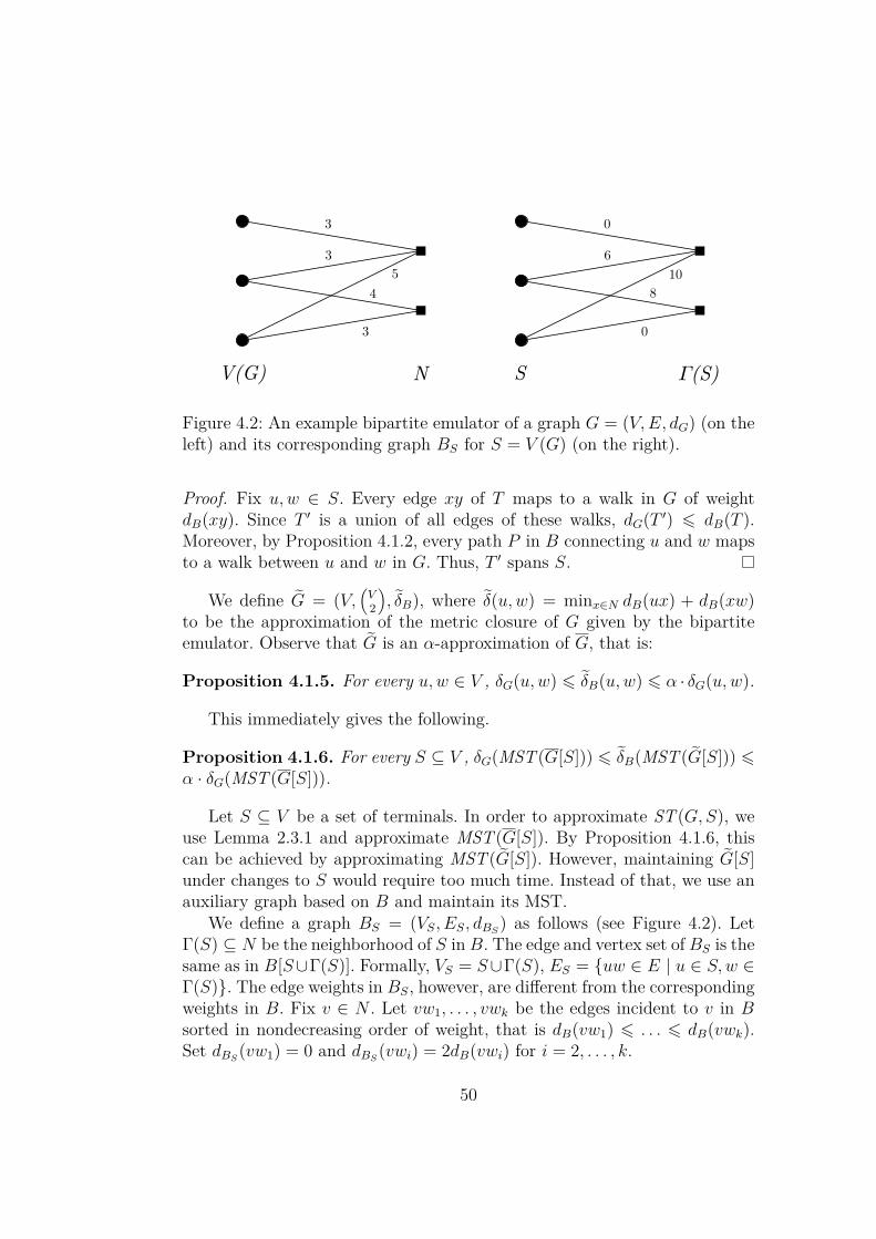
Figure 4.2: An example bipartite emulator of a graph G = (V,E, dG) (on theleft) and its corresponding graph BS for S = V (G) (on the right).

Proof. Fix u,w ∈ S. Every edge xy of T maps to a walk in G of weightdB(xy). Since T ′ is a union of all edges of these walks, dG(T ′) ¬ dB(T ).Moreover, by Proposition 4.1.2, every path P in B connecting u and w mapsto a walk between u and w in G. Thus, T ′ spans S.

We define G = (V,(

V2

), δB), where δ(u,w) = minx∈N dB(ux) + dB(xw)

to be the approximation of the metric closure of G given by the bipartiteemulator. Observe that G is an α-approximation of G, that is:

Proposition 4.1.5. For every u,w ∈ V , δG(u,w) ¬ δB(u,w) ¬ α · δG(u,w).

This immediately gives the following.

Proposition 4.1.6. For every S ⊆ V , δG(MST (G[S])) ¬ δB(MST (G[S])) ¬α · δG(MST (G[S])).

Let S ⊆ V be a set of terminals. In order to approximate ST (G,S), weuse Lemma 2.3.1 and approximate MST (G[S]). By Proposition 4.1.6, thiscan be achieved by approximating MST (G[S]). However, maintaining G[S]under changes to S would require too much time. Instead of that, we use anauxiliary graph based on B and maintain its MST.

We define a graph BS = (VS, ES, dBS) as follows (see Figure 4.2). Let

Γ(S) ⊆ N be the neighborhood of S in B. The edge and vertex set of BS is thesame as in B[S∪Γ(S)]. Formally, VS = S∪Γ(S), ES = uw ∈ E | u ∈ S,w ∈Γ(S). The edge weights in BS, however, are different from the correspondingweights in B. Fix v ∈ N . Let vw1, . . . , vwk be the edges incident to v in Bsorted in nondecreasing order of weight, that is dB(vw1) ¬ . . . ¬ dB(vwk).Set dBS

(vw1) = 0 and dBS(vwi) = 2dB(vwi) for i = 2, . . . , k.

50

Let us now provide some intuition behind this construction. As we latershow, this choice of edge weights assures that the distances between verticesof S in BS are at most twice the distances in B, and at the same time, theyare not smaller than the distances in B. Moreover, in BS, every vertex ofΓ(S) is connected to a vertex of S with an edge of weight 0. This meansthat any tree spanning S in BS can be extended to a spanning tree of BS

of the same weight. Thus, MST (BS) and ST (BS, S) have the same weight,and because the distances in BS approximate distances in G, we may useMST (BS) to approximate ST (G,S).

In our algorithm we maintain the MST of BS. Our entire construction canbe described by the following sequence of trees. Each object in the sequenceis used to approximate the previous one: Steiner tree in G, MST (G[S]),MST (G[S]), tree spanning S in B, MST (BS). We first show how to relateweight of MST (BS) to a weight of a tree spanning S in B.Lemma 4.1.7. Let T be a tree in BS, which does not contain any leaves inΓ(S). Then dB(T ) ¬ dBS

(T ).Proof. Let us group the edges of T by their endpoints in N and show theinequality for each group. Fix v ∈ Γ(S), such that v belongs to T . Letvw1, . . . , vwk be the edges of T incident to v, ordered such that dBS

(vw1) ¬. . . ¬ dBS

(vwk). We assume that if T contains the edge that is assignedzero weight during the construction of GS, it comes first in this order. Thus,dBS

(vwi) = 2dG(vwi) for all 2 ¬ i ¬ k. In addition, since no vertex of N is aleaf, k ­ 2. Hence,

dBS(vw1) + . . .+dBS

(vwk) ­ dBS(vw2) + . . .+ dBS

(vwk)= 2(dG(vw2) + . . .+ dG(vwk))­ (dG(vw1) + dG(vw2)) + 2(dG(vw3) + . . .+ dG(vwk))­ dG(vw1) + . . .+ dG(vwk).

Lemma 4.1.8. dBS(MST (BS)) ¬ 2δB(MST (G[S])).

Proof. We map each edge of MST (G[S]) to a corresponding two-edge pathin BS, thus obtaining a tree Tn. Note that dB(Tn) ¬ δB(MST (G[S])), asmultiple paths can contain the same edge of B. Observe that vertices of Tn

are contained in S∪Γ(S), so Tn is also a tree in BS. Since for any uw ∈ E(BS),dBS

(uw) ¬ 2dB(uw), we have that dBS(Tn) ¬ 2dB(Tn) ¬ 2δB(MST (G[S])).

Moreover, every v ∈ N in BS is connected to a vertex of S with a zero-weight edge, so by adding zero-weight edges to Tn, we can obtain a treeT such that dBS

(T ) = dBS(Tn) and T is a spanning tree of BS. We have

dBS(MST (BS)) ¬ dBS

(T ) = dBS(Tn) ¬ 2δB(MST (G[S])).

51

The following lemma shows that the MST of BS can be used to approxi-mate ST (G,S). The weight of MST (BS) is low and it maps to a tree spanningS in G of weight at most dBS

(MST (BS)).

Lemma 4.1.9. Let T be a tree obtained from MST (BS) by removing allleaves that are vertices of Γ(S). Then, T maps to a subgraph T ′ spanning Sin G, and dG(T ′) ¬ dBS

(MST (BS)) ¬ 4α · dG(ST (G,S)).

Proof. Let v ∈ Γ(S) be a leaf of MST (BS). Since every vertex of Γ(S) isconnected to a vertex of S with an edge of weight 0, the weight of the onlyedge incident to v is also 0. Thus, dBS

(T ) = dBS(MST (BS)). Clearly, T is a

tree that spans S in BS and in B. By Lemma 4.1.4, T maps to a subgraphT ′ of G spanning S. We have

dBS(MST (BS)) = dBS

(T )­ dB(T ) by Lemma 4.1.7­ dG(T ′) by Lemma 4.1.4

It remains to show the last inequality:

dBS(MST (BS)) ¬ 2δB(MST (G[S])) by Lemma 4.1.8

¬ 2α · δG(MST (G[S])) by Proposition 4.1.6¬ 4α · dG(ST (G,S)) by Lemma 2.3.1

Lemma 4.1.10. Let G = (V,E, dG) be a graph and let B = (V ∪N,EB, dB, p)be its bipartite emulator with stretch α. Denote by ∆ the maximum degree ofa vertex from V in B. Let S be a set subject to insertions and deletions, suchthat at any time S ⊆ V . Then, we can maintain a 4α-approximate Steinertree of G that spans S, handling each update to S in O(∆ log4 n) time.

Proof. From Lemma 4.1.9 it follows that it suffices to maintain MST (BS).In order to do that, as the elements are inserted to or removed from S,we maintain the graph BS and run the decremental MSF algorithm (seeTheorem 2.3.2) on top of it. This algorithm requires O(log4 n) amortizedtime for any edge addition or removal.

Recall that the edge and vertex sets of BS are the same as in B[S ∪Γ(S)]. Thus, each time a vertex is added to/removed from S, we need to

52

insert/remove a single vertex from BS and all its incident edges. For simplic-ity, instead of adding/removing a vertex, we may add/remove all its incidentedges.

It remains to describe how to maintain the edge weights of BS. Recall thatfor each v ∈ N , the edge incident to v in BS that has the smallest weight inB, has weight 0 in BS. Other edges incident to v have weight which is twotimes bigger than their weight in B. It is easy to see that adding/removinga single edge to BS may trigger one edge weight update. In order to detectthese updates, for every v ∈ N we maintain a heap containing the weights ofall its incident edges.

It follows that handling an update to S requires O(∆) edge updates in thegraph BS that we maintain. Thus, updating MST (GS) requires O(∆ log4 n)amortized time. We also need O(log n) per each change to detect edge weightupdates, but this time is dominated by the time needed to maintain theMST.

4.2 Constructing Bipartite EmulatorsIn this section we show how to construct emulators that can be plugged intoLemma 4.1.10 to obtain dynamic algorithms for maintaining the Steiner tree.

4.2.1 General GraphsOur bipartite emulator for general graphs is based on an approximate dis-tance oracle by Thorup and Zwick [44]. Let G = (V,E, dG) be an undirected,weighted graph, and k ­ 1 be an integer. The algorithm first constructs asequence of sets A0 ⊇ A1 ⊇ . . . ⊇ Ak−1 ⊇ Ak. We set A0 = V . For 1 ¬ i < k,Ai is obtained by taking each element of Ai independently with probabil-ity n−1/k, and Ak = ∅. We assume that Ak−1 6= ∅. This happens with bigprobability, so we can assure it by repeating the sampling, if necessary.

For a v ∈ V , we define a bunch of v to be a set B(v) = ⋃k−1i=0 w ∈

Ai \ Ai+1 | δG(w, v) < δG(Ai+1, v). Here, δG(Ai+1, v) denotes the distancebetween v and the nearest vertex in Ai+1. Moreover, for v ∈ V , and 0 ¬ i < k,we define pi(v) to be the vertex in Ai, which is nearest to v.

The initialization of the oracle consists in computing:

• the sets A0, . . . , Ak,

• the bunch B(v) for every v ∈ V ,

• pi(v) for every v ∈ V and 0 ¬ i < k,

53

• the distance δG(v, pi(v), for every v ∈ V and 0 ¬ i < k,

• the distance δG(u,w) for every w ∈ B(u).

Let us now list some properties of the oracle that we use.

Lemma 4.2.1 ([44]). Let G = (V,E, d) be a graph, n = |V |, m = |E|, andk ­ 1 be an integer. Then, the approximate distance oracle can be initializedin O(kmn1/k) expected time.

Lemma 4.2.2 ([44]). Let v1, v2 ∈ V . For some s ∈ 1, 2, there exists avertex x ∈ B(vs), such that x = pj(v3−s) for some 0 ¬ j < k and δG(v1, x) +δG(x, v2) ¬ (2k − 1)δG(v1, v2).

Lemma 4.2.3 ([44]). For every v ∈ V , the expected size of B(v) is O(kn1/k).

Observe that the distances δG(v1, x) and δG(x, v2) are computed duringthe initialization of the oracle.

Lemma 4.2.4. Let G = (V,E, d) be a graph, n = |V |, m = |E|, and k ­ 1be an integer. We can compute a bipartite emulator B = (V ∪ N,EB, dB, p)of G of stretch 2k−1 in O(kmn1/k) expected time. The degree of every vertexof V in B is O(n1/k).

Proof. By Lemma 4.2.1, we build a TZ oracle for G in O(kmn1/k) expectedtime. Let V ′ be a copy of V . For each vertex v ∈ V , V ′ contains its copy v′.We set the vertex set of B to be V ∪ V ′.

Now, for every u,w, such that u ∈ V and w ∈ B(u), we add to B an edgeuw′ of weight δG(u,w). Moreover, for every u ∈ V and 0 ¬ i < k, we add toB an edge upi(u)′ of weight δG(u, pi(u)). Note that the distances we need arecomputed during the initialization of the oracle.

We now prove that we obtain a bipartite emulator. Consider u,w ∈ V . ByLemma 4.2.2, there exists x ∈ B(w), such that (possibly after we swap u andw) x = pj(u) for some 0 ¬ j < k and δG(u, x) + δG(x,w) ¬ (2k− 1)δG(u,w).Observe that B contains edges ux′ and wx′ of lengths δG(u, x) and δG(w, x),respectively. Thus, there is a two-edge path in B between u and w of lengthat most (2k − 1)δG(u,w). It is easy to see that for every v′ ∈ V ′, we setp(v′) = v, to obtain the desired mapping between V ′ and V .

The expected degree of every v ∈ V in B is O(|B(v)| + k), which, byLemma 4.2.3 is O(kn1/k) The initialization time is clearly dominated by thetime needed to construct the TZ oracle.

By combining the above Lemma with Lemma 4.1.10 we obtain the fol-lowing result.

54

Theorem 4.2.5. Let G = (V,E, d) be a graph, n = |V |, m = |E| and k ­ 1be an integer. Let S ⊆ V be a dynamic set, subject to vertex insertions andremovals (initially S = ∅). Then, after preprocessing in O(kmn1/k) expectedtime, we may maintain a (8k − 4)-approximate Steiner tree that spans S,handling each update to S in O(kn1/k log4 n) expected amortized time.

4.2.2 Planar GraphsIn this section we show a construction of a bipartite emulator for planargraphs. As a result we obtain an algorithm which maintains a (4 + ε)-approximate Steiner tree in polylogarithmic time per update. In order toreach this goal, we use a construction by Thorup (Section 3.8 in [43]) thatwe extend in order to construct a bipartite emulator (see Lemma 4.2.7).

Let G = (V,E, dG) be an undirected weighted planar graph. The overallidea uses recursive division of G using balanced separators. We find a bal-anced separator of G that consists of a constant number of shortest pathsP1, . . . , Pk (the separator consists of vertices contained in these paths). Fora shortest path Pi, we build an emulator that approximates all the short-est paths in G that intersect Pi. Then, we recurse on each of the connectedcomponents of G \ (P1 ∪ . . . ∪ Pk). Hence, we now focus on the followingproblem. Given a planar graph G and a shortest path P , build an emulatorthat approximates all shortest paths intersecting P .

We define a connection to be an edge that connects a vertex v ∈ Vwith a vertex a ∈ P and has length dG(va), which is at least δG(v, a) (itwould be convenient to assume that dG(va) = δG(v, a), but the algorithm weuse may sometimes give longer connections). A connection vb ε-covers x ifdG(vb) + δG(b, x) ¬ (1 + ε)δG(v, x). Observe that the distance δG(b, x) canbe measured along the path P . A set of connections C(v, P ) between v ∈ Vand P is ε-covering if it ε-covers every x ∈ P .

Lemma 4.2.6. Let G = (V,E, dG) be a planar graph, n = |V |, and 0 < ε ¬1. Let P be a shortest path in G. For each v ∈ V (G) we can construct anε-covering set C(v, P ) of size O(ε−1) in O(ε−1n log n) total time.

A very similar fact is shown in [43], but the definition of ε-covering usedthere is slightly different, so, for the sake of completeness, we rewrite theproof.

Proof. Let ε0 = ε/2. We say that a connection vb strongly-ε-covers a ifdG(vb) + (1 + ε)δG(b, a) ¬ (1 + ε)δG(v, a). By Lemma 3.18 in [43], for eachv ∈ V (G) we can construct a strongly-(ε0/2)-covering set D(v, P ) of size

55

O(ε−10 log n) in O(ε−1

0 n log n) time.1 We now show that we can use it toconstruct an ε-covering set C(v, P ) ⊆ D(v, P ) of size O(ε−1).

Let vc be the shortest connection from D(v, P ) and s be one of the twoendpoints of P . We add vc to C(v, P ). Now, iterate through connections inD(v, P ) starting from vc and going towards s. Let vb be the connection thatwas most recently added to C(v, P ). If for the current connection va we havedG(vb) + δG(b, a) > (1 + ε0)dG(va), we add va to C(v, P ). Then, we run asimilar procedure using the other endpoint of P .

To prove that C(v, P ) covers every vertex between c and s, consider somevertex x ∈ P . There exists a connection va ∈ D(v, P ) that strongly-(ε0/2)-covers vx, so dG(va)+(1+ε0/2)δG(a, x) ¬ (1+ε0/2)δG(v, x). If this connectionis in C(v, P ) then vx is strongly-ε0/2-covered and obviously also ε-covered.Otherwise, there exists a connection vb such that dG(vb) + δG(b, a) ¬ (1 +ε0)dG(va). We have

dG(vb) + δG(b, x) ¬ dG(vb) + δG(b, a) + δG(a, x)¬ (1 + ε0)dG(va) + δG(a, x)¬ (1 + ε0)dG(va) + (1 + ε0)(1 + ε0/2)δG(a, x)= (1 + ε0)(dG(va) + (1 + ε0/2)δG(a, x))¬ (1 + ε0)(1 + ε0/2)δG(v, x)¬ (1 + ε)δG(v, x).

The last inequality follows from ε0 = ε/2 ¬ 1. It remains to bound the size ofC(v, P ). Let f(vb) = dG(vb) + δG(b, s). As connections are added to C(v, P )we trace the value of f(vb), where vb is the last connection that we haveadded. Every time we add a connection va we reduce the value of f by

f(vb)− f(va) = dG(vb) + δG(b, s)− dG(va)− δG(a, s)= dG(vb)− dG(va) + δG(b, a)> ε0dG(va)­ ε0δG(v, c).

However, the total change equals

f(vc)− f(vs) = dG(vc) + δG(c, s)− dG(vs)¬ (1 + ε0)δG(v, c) + δG(c, s)− δG(v, s)¬ (2 + ε0)δG(v, c).

1Strictly speaking, the strongly-ε-covering set according to our definition is an ε/(ε+1)-covering set according to the definition used in the statement of Lemma 3.18 of [43].

56

Thus, at most O(ε−10 ) = O(ε−1) connections are added to C(v, P ).

The same procedure is then repeated for the other endpoint of P , so weget a total of O(ε−1) connections.

Lemma 4.2.7. Let G = (V,E, dG) be a planar graph, n = |V |, 0 < ε ¬ 1.Let P be a shortest path in G. For each v ∈ V we can construct a set ofconnections C ′(v, P ) of size O(ε−1 log n), which satisfies the following prop-erty. For any two vertices u,w ∈ V , if the shortest path between u and wintersects P , then for some x ∈ P there exist connections ux ∈ C ′(u, P ) andwx ∈ C ′(w,P ), such that δ(u,w) ¬ dG(ux) + dG(wx) ¬ (1 + ε)δ(u,w). Thesets C ′(v, P ) can be constructed in O(ε−1n log n) time.

Proof. First, using Lemma 4.2.6, for every v ∈ V we construct an ε-coveringsets of connections C(v, P ). Consider a shortest path Q between u and w,which intersects P in x ∈ P . There exists a path Q′ between u and w whichconsists of a connection, subpath of P , denoted henceforth Q′P , and anotherconnection. Moreover, dG(Q′) ¬ (1+ε)dG(Q). We call each path of this forman approximating path. Our goal is to substitute every approximating pathwith an approximating path that consists solely of two connections fromC ′(v, P ).

The construction is done recursively. The parameter of the recursion is asubpath P ′ of P . Consider a single step, with a parameter P ′ = p1p2 . . . pk.Let pm = pbk/2c be the middle vertex of P ′. For any v ∈ V and pi ∈ P ′,if there is an connection vpi ∈ C(v, P ), we add a connection vpm of lengthdG(vpi) + δ(pi, pm) to C ′(v, P ). Then, we recurse on P1 = p1p2 . . . pm−1 andP2 = pm+1 . . . pk. Lastly, for each pi ∈ P we add a connection pipi of length0.

To prove the correctness of the procedure, consider now the aforemen-tioned approximating path Q′, and recall that Q′P = P ∩ Q′. Let p be thevertex that is taken as pm in the closest to root node in the recursion tree ofthe algorithm, among all vertices of Q′P . Observe that in the single recursivestep when pm = p, we add to C ′(v, P ) the connections up and wp of lengthexactly equal to the length of the part of Q′ between u and p, and the partof Q′ between p and w, respectively. Also, the connections we add clearly donot cause any distances to be underestimated.

The running time of each step is proportional to the length of the sub-path we consider and the number of connections incident to this subpath.Moreover, every connection may be considered in at most O(log n) recursivecalls, so we we add to C ′(v, P ) at most O(ε−1 log n) connections. It followsthat the total running time of the procedure is O(ε−1n log n).

57

Lemma 4.2.8. Let G = (V,E, d) be a planar graph, n = |V |, 0 < ε ¬ 1.We can construct a bipartite emulator B = (V ∪N,EB, dB, p) of G of stretch1 + ε. The degree of every v ∈ V in B is O(ε−1 log2 n). The graph B can beconstructed in O(ε−1n log2 n) time.

Proof. We begin with B being a graph with vertex set V and no edges. Theconstruction is done recursively. As it is shown, e.g., in [43], each planargraph admits a balanced separator that consists of a constant number ofshortest paths P1, . . . , Pk, and, moreover, such a separator can be found inO(n) time. For each path Pi we use Lemma 4.2.7 to construct a set of con-nections C ′(v, Pi) for every v ∈ V . Next, we iterate through the vertices ofthe paths Pi. For each vertex w ∈ Pi we add a new auxiliary vertex w′ to Band add an edge uw′ for each connection uw from G (the length of the edgeis the length of the connection). After that, we recurse on each connectedcomponent of G \ (P1 ∪ . . . ∪ Pk).

Let us now prove the correctness of the construction. Consider any twov1, v2 ∈ V and the shortest path Q between them. At some step of therecursion, some vertex of Q belongs to the separator that we have found.From the construction, it follows that in this step we have added to B a vertexw′ and edges v1w

′ and v2w′ to B of total length at most (1 + ε)δG(v1, v2). It

remains to prove that B has the second property of the bipartite emulator.It follows from the fact that each time we add a vertex w′ and connectionuw′, w′ corresponds to some vertex of V and the connection has length equalto the length of some walk between u and the corresponding vertex of w′.

Since every vertex v ∈ V takes part in O(log n) recursive steps and inevery step we add O(ε−1 log n) edges incident to any v ∈ V , we have that thedegree of any vertex of V in B is O(ε−1 log2 n). As shown in [43], finding theseparators requires O(n log n) total time. The running time of every recursivestep is dominated by the time from Lemma 4.2.7. Summing this over allrecursive steps, we get that the construction can be done in O(ε−1n log2 n)time.

By constructing B according to Lemma 4.2.8 and applying Lemma 4.1.10we obtain the following.

Theorem 4.2.9. Let G = (V,E, d) be a planar graph and 0 < ε ¬ 1. LetS ⊆ V be a dynamic set, subject to vertex insertions and removals (initiallyS = ∅). Then, after preprocessing in O(ε−1n log2 n) time, we may maintaina (4 + ε)-approximate Steiner tree that spans S, handling each update to Sin O(ε−1 log6 n) amortized time.

58

4.3 Related ResultsIn the paper by Łącki et al. [31], in addition to the algorithm for dynamicSteiner tree, which we present in this chapter, other results are obtained.Namely, the paper shows that it is possible to obtain better approximationratios, if we allow higher running time. In particular, it presents a (6 + ε)-approximate algorithm, which for a weighted graph G = (V,E, dG) processesupdates in O(ε−5√n logD) amortized time. Here, D is the stretch of G, thatis the ratio between the weights of edges with maximal and minimal weights.Moreover, for planar graphs, two (2 + ε)-approximate algorithms are shown.The first one processes updates in O(ε−5.5√n logD) amortized time. Thesecond one handles each update in O(ε−2 log3 n logD) amortized time, butit only supports adding terminals. While this approximation ratios are twotimes smaller than the ones we have obtained in this chapter, they are stillfar from what can be computed in polynomial time in static case. In generalgraphs, a 1.39-approximate algorithm is known [8], whereas for planar graphsthere exists a PTAS [7]. We believe that there exist dynamic algorithmswith lower approximation ratios, and designing them is an interesting openproblem.

59

Chapter 5

Connectivity in GraphTimelines

In this section we consider dynamic connectivity in undirected graphs in asemi-offline model. We develop algorithms that process a graph timeline, thatis a sequence of graphs G1, . . . , Gt, such that Gi+1 is obtained from Gi byadding or removing a single edge. In this model, an algorithm may preprocessthe entire timeline at the beginning, and after that it should answer queriesarriving in online fashion. We consider timelines of undirected graphs and twotypes of queries. Moreover, in order to obtain simpler running time boundswe assume t = O(nc).

An exists(u,w, a, b) query, where u and w are vertices and 1 ¬ a ¬ b ¬ t,asks whether vertices u and v are connected in any of Ga, Ga+1, . . . , Gb. Weshow an algorithm that after preprocessing in O(m + nt) time may answersuch queries in O(1) time.

We also consider a forall(u,w, a, b) query, which asks whether vertices uand v are connected in all graphs among Ga, Ga+1, . . . , Gb. For this problem,we show an algorithm whose preprocessing time is O(m+ t log t log log t) (mdenotes the number of edges in G1) and the query time is O(log n log log t).The algorithm is randomized and answers queries correctly with high prob-ability.

In the following part of this chapter, we first introduce a data structure,which is common to the algorithms handling both types of queries (Sec-tion 5.1). In Section 5.2 we present an algorithm answering exists queries.Then, in Section 5.3 we deal with forall queries. Finally, in Section 5.4,we discuss the recent improvements to our algorithms that were made byKarczmarz [27].

60

5.1 Connectivity History TreeIn this section we introduce a data structure, which represents connectiv-ity information of the entire timeline. We begin by introducing some basicnotation related to graph timelines.

Let G1 = (V,E1), G2 = (V,E2) be two undirected graphs on the samevertex set. We define their intersection G1 ∩ G2 to be a graph G′ obtainedby intersecting the sets of their edges, that is G′ = (V,E1 ∩E2). Let Gt be agraph timeline. For an interval1 [a, b], we define G[a,b] := Ga∩Ga+1∩ . . .∩Gb.We say that an edge is permanent if it is an edge of G[1,t], that is, it ispresent in every graph in the timeline. Other edges of the timeline are calledtemporary. If an edge connecting two vertices is removed from the timeline,and then added again, we consider these two edges different. This allows usto define a lifetime of an edge to be the maximal (w.r.t. inclusion) interval[a, b], such that the edge is present in all graphs Ga, . . . , Gb.

We assume that the input timeline is represented in O(m + t) space,where m denotes the number of edges of G1. The representation consists ofthe representation of G1, and, for each 2 ¬ i ¬ t, the information about theedge that is added or removed to obtain Gi.

Proposition 5.1.1. There are at most m permanent edges and t temporaryedges. We can compute the lists of permanent and temporary edges in O(m+t)time.

We first show that we may reduce our problems to the case when thegraph timeline does not contain any permanent edges. The reduction takesonly linear time.

Lemma 5.1.2. Assume there exists an algorithm that, given a graph time-line Gt with no permanent edges, after preprocessing in f(n, t) time an-swers exists / forall queries in g(n, t) time, where g(n, t) and f(n, t)are nondecreasing in both parameters. Then, there exists an algorithm that,given a graph timeline that may contain permanent edges, after preprocess-ing in f(min(n, 2t), t) +O(m+ t) time answers exists / forall queries ing(min(n, 2t), t) +O(1) time.

Proof. We build a graph timeline Gt, which does not contain permanentedges and can be used to answer queries regarding Gt. Observe that twovertices u and w connected with a path consisting of permanent edges areequivalent from the point of view of exists and forall queries. Thus, wecan contract all permanent edges.

1Throughout this chapter we assume that the intervals are intervals of integers.

61

By Proposition 5.1.1, we can find all permanent edges in O(m+ t) time.Let V be the set of vertices of the graphs in the timeline. We build a graphH consisting a vertex set V and all permanent edges. Then, we computeconnected components of H in O(m+ t) time. Denote by cc[v] the connectedcomponent of a vertex v ∈ V .

Consider a connected component C of H. We say that C is volatile, ifsome temporary edge is incident to a vertex of C. Assume v is a vertex ofa non-volatile component C. Then, v is connected to other vertices of C inall graphs in the timeline, and is not connected to the remaining verticesin every graph in the timeline. Thus answering queries about the timeline,where at least one of the parameters is a vertex of a non-volatile componentis simple, if we store the non-volatile components of H

To answer the remaining queries, we build a new timeline Gt. Each vertexof each graph of Gt is a volatile connected component of H. For every tem-porary edge uw of Gt, whose both endpoints belong to volatile components,we add an edge cc[u]cc[w] to Gt. In order to answer a query regarding twovertices u and w in Gt, that both belong to volatile components, we issue thesame query about vertices cc[u] and cc[w] in Gt.

It remains to show that Gt consists of graphs on at most 2t vertices. Thisfollows from the fact that each volatile component contains an endpoint of atemporary edge, and the temporary edges have 2t endpoints in total.

Hence, in the following part of this chapter, we assume that we work witha timeline with no permanent edges, and t = Ω(n). Both these properties canbe assured in linear time, by applying Lemma 5.1.2.

We now define a data structure, which is used in the algorithms for bothexists and forall queries. Throughout the following part of this chapter weheavily use the properties of segment trees (see Section 2.2) and disjoint-setdata structures (see Section 2.3.3).

Definition 5.1.3. Let t be a power of 2 and let Gt be graph timeline. Aconnectivity history tree (CHT) for Gt is a is a segment tree with t leaves.For each elementary interval [a, b] of the segment tree, it contains a DSDSC[a,b] of the graph G[a,b].

Figure 5.1 shows an example of graphs G[a,b] for all elementary intervals.In Figure 5.2, there is the corresponding CHT containing a DSDS C[a,b] forevery elementary interval [a, b]. For an elementary interval [a, b], we defineD[a,b] to be the list of edges such that G[a,b] is obtained from GParent([a,b]) byadding edges of D[a,b]. If [a, b] has no parent, we let D[a,b] be the list of edgesof G[a,b].

62

Figure 5.1: The timeline G1, G2, G3, G4 and the corresponding graphs G[a,b]for all elementary intervals [a, b], arranged into a tree. Note that for i =1, 2, 3, 4, Gi = G[i,i].

Figure 5.2: The CHT corresponding to the timeline from Figure 5.1. Witheach elementary interval we associate a DSDS. The arrows in each node pointfrom a vertex to its parent in the DSDS. Parent pointers of the representativeshave been omitted.

63

In the example from Figure 5.1, we have D[1,2] = vw, D[2,2] = vx, D[3,4] =vx, wy, D[3,3] = vw. The remaining lists, D[1,4], D[1,1] and D[4,4], are empty.

Lemma 5.1.4. Let Gt be a graph timeline with no permanent edges. We cancompute the lists D[a,b] for all elementary intervals [a, b] in O(t log t) time.The total length of the lists is O(t log t).

Proof. The algorithm is very simple. Consider a temporary edge e, whoselifetime is [c, d]. We use Lemma 2.2.8 to decompose [c, d] into k = O(log t)elementary intervals [a1, b1], . . . , [ak, bk] and add e to D[ai,bi] for 1 ¬ i ¬ k.Since the number of temporary edges is O(t), this takes O(t log t) time andthe total length of the resulting lists is O(t log t). It remains to show thecorrectness of our construction.

First, we need to show that every edge belonging to the list D[a,b] com-puted this way is an edge of G[a,b] = Ga ∩ Ga+1 ∩ . . . ∩ Gb. This followsdirectly from the construction. An edge is added to D[a,b] only if its lifetimeis an interval [c, d] ⊇ [a, b]. Second, we need to show that every edge of G[a,b]is contained either in D[a,b] or GParent([a,b]). Consider an edge e ∈ E(G[a,b]).Let the lifetime of e be [c, d]. Clearly [a, b] ⊆ [c, d]. By Lemma 2.2.9, thedecomposition of [c, d] into elementary intervals either contains [a, b] or oneof its ancestors. In the first case, e is added to D[a,b], whereas in the secondcase Parent([a, b]) ⊆ [c, d], so e ∈ GParent([a,b]). The lemma follows.

5.2 exists QueriesWe now describe an algorithm for answering exists queries. We first com-pute an explicit representation of the CHT.

Lemma 5.2.1. Let Gt be a graph timeline with no permanent edges. TheCHT of Gt can be computed in O(nt) time. It uses O(nt) space.

Proof. We first use Lemma 5.1.4 to compute lists D[a,b] for all elementaryintervals [a, b] in O(t log t) time. Then, we can compute the DSDSes C[a,b] ina top-down fashion. Since there are no permanent edges, G[1,t] consists solelyof isolated vertices, so computing C[1,t] is trivial.

Then, we compute C[a,b] by first creating a copy of CParent([a,b]) and thenadding edges ofD[a,b] to it. It takesO(n) time to create each of theO(t) copies.Moreover, we add O(t log t) edges from lists D[a,b], each in time O(log n). Thisgives O(t log t log n) total time, which is O(nt), since we assume t = O(nc).The lemma follows.

64

In order to answer queries, our algorithm precomputes, for all elemen-tary intervals [a, b], and all pairs of vertices u and v, the answer to anexists(u, v, a, b) query. Thus, by Lemma 2.2.8, the answer to a query re-garding an arbitrary interval [p, q] can be computed in O(log t) time by de-composing [p, q] into O(log t) elementary intervals and combining the answersfor these intervals. However, as we later show, this can be improved to con-stant time.

For each elementary interval [a, b], we compute a two-dimensional Booleanmatrix M[a,b] which contains answers to exists(u, v, a, b) queries for all pairsof vertices u, v. The matrix is indexed by vertices of the graph. We set[M[a,b]]u,v = 1 if and only if u and v are connected in any of Ga, . . . , Gb.Additionally, for each node in the CHT, we define matrices F[a,b] and L[a,b].If [M[a,b]]u,v = 1, then [F[a,b]]u,v is equal to the index of the first graph amongGa, . . . , Gb, in which u and v are connected. Otherwise, [F[a,b]]u,v is set to∞.The matrix L[a,b] is defined similarly, but it contains indices of the last graph,in which the vertices are connected (thus, we use −∞ instead of ∞).

We now show that these matrices can be computed and stored efficientlyin a way that allows constant-time access to each of their cells.

Lemma 5.2.2. Let Gt be a graph timeline with no permanent edges. We cancompute implicit representations of the matrices M[a,b], F[a,b] and L[a,b] forall elementary intervals [a, b] in O(nt) time. The representations use O(nt)space.

Proof. For each elementary interval [a, b], CHT contains C[a,b], which is aDSDS representing G[a,b]. By Proposition 2.3.7, given a DSDS of an n-vertexgraph G, we may compute its connected components in O(n) time. Thisallows us to compute, for every elementary interval [a, b], the connected com-ponents of G[a,b] in O(nt) total time.

We now describe the implicit representation of matrices M[a,b]. If b−a > n,M[a,b] is stored explicitly as a n× n matrix. However, if b− a ¬ n, then thematrix has a more compact implicit representation, as some of its rows orcolumns are equal to each other. Consider a connected component C of G[a,b].Vertices belonging to C are connected in each of Ga, Ga+1, . . . , Gb. Hence,it suffices only to store one row and column of M[a,b] for each connectedcomponent C.

Furthermore, within Ga, . . . , Gb at most b−a edges are added or deleted.The endpoints of these edges are contained in at most 2(b − a) = O(b − a)components of G[a,b]. We call these components volatile. Denote the numberof volatile components by s and choose a single representative vertex fromeach of them, thus obtaining a list v1, . . . , vs.

Thus, it suffices to store:

65

• an s × s submatrix of M[a,b] containing only rows and columns corre-sponding to v1, . . . , vs,

• for each v ∈ V , the identifier of its connected component in G[a,b],

• for each v ∈ V , whether it belongs to a volatile component,

• for each v ∈ V belonging to a volatile component, the representativevertex from this component.

Using this representation, we may obtain the value of any cell of M[a,b]in the following way. Consider two vertices u and w. First, assume that atleast one of them (say u) does not belong to a volatile component. Let C bethe connected component of u in G[a,b]. Since C is not volatile, the connectedcomponent of u is equal to C in every element of Ga, . . . , Gb. Hence, it sufficesto check whether u and w are connected in G[a,b].

Otherwise, if u and w both belong to volatile components, we find therepresentative vertices vi and vj of u and w. Then, we simply check the valueof [M[a,b]]vi,vj

, which is stored explicitly. Overall, the implicit representationof M[a,b] takes O(min((b− a)2, n2) + n) space.

The implicit representation of all matrices M[a,b] can be simply computedin time that is linear in their size. We proceed in a bottom-up fashion on thesegment tree. For a leaf interval [a, a], there are no volatile components, sowe simply store identifiers of connected components, which we have alreadycomputed. Now consider a non-leaf interval [a, b], and b − a ¬ n. First,note that we have computed the identifiers of connected components of G[a,b]before. In order to find volatile components, we simply iterate through alledges that are added or deleted in the interval [a, b], which takes O(b− a) =O(n) time. Then, we compute representative vertices in O(n) time. Finally,we compute the s× s submatrix of M[a,b]. Observe that

[M[a,b]]x,y = max([MLeft([a,b])]x,y, [MRight([a,b])]x,y), (5.1)

and this expression can be evaluated in constant time (since the implicit rep-resentations of MLeft([a,b]) and MRight([a,b]), which allow constant-time access,have already been computed). Thus, the implicit representation of M[a,b] iscomputed in O(min((b − a)2, n2) + n) time. It remains to consider the casewhen b − a > n, but then we simply compute an n × n matrix using For-mula 5.1.

Observe that the implicit representations of F[a,b] and L[a,b] can be com-puted in an analogous way. Let us focus on F[a,b]. If two vertices u and ware connected in G[a,b], we set [F[a,b]]u,w = a. If they stay disconnected in

66

every graph among Ga, . . . , Gb, we set [F[a,b]]u,w =∞. Otherwise we can usea formula [F[a,b]]x,y = min([FLeft([a,b])]x,y, [FRight([a,b])]x,y).

It remains to bound the total running time and space usage. Assume thatt = 2d. There are 2d−i elementary intervals containing 2i elements. For eachsuch interval, the running time is O(min(22i, n2) + n). Thus, we have

d∑i=0

2d−i(min(22i, n2) + n) =d∑

i=02d−in+

blog nc∑i=0

2d−i22i +d∑

blog nc+12d−in2

=nt+blog nc∑

i=02d+i + 2dn2

d∑blog nc+1

2−i

=nt+ 2dO(n) + 2dn2O(1/n) = O(nt).

Note that we have used an assumption that log n ¬ d, which follows fromn ¬ t, but this was for convenience only. We can derive the same bound inthe case when t = Ω(n).

5.2.1 Answering QueriesAfter the preprocessing phase, a query regarding an interval [a, b] can beanswered by decomposing it into O(log t) elementary intervals. The matricesM[a,b] allow us to obtain the answer for every elementary interval in O(1)time, so each query requires O(log t) total time. However, this can be alsodone faster. We show how to use matrices F[a,b] and L[a,b] to improve thequery time to O(1).

Moreover, it is possible to extend the algorithm, so that it reports thegraphs in which the two given vertices are connected. This can be doneoptimally, i.e., the graphs can be returned one by one, each with constantdelay.

Let Parity(x) := maxi 2i | x and MaxParity(a, b) be the number fromthe interval [a, b] that maximizes the value of Parity.

Proposition 5.2.3. For any 1 ¬ a ¬ b, the value of MaxParity(a, b) isuniquely defined.

Proof. Assume that Parity(x) = Parity(y) and a ¬ x ¬ y ¬ b. Letz := x + 2Parity(x). Clearly, Parity(z) > Parity(x). Moreover, z is thesmallest element greater than x, such that Parity(z) ­ Parity(x). Thus,z < y, so a ¬ z ¬ b. Hence, if Parity(x) = Parity(y), there exists z, suchthat x < z < y and Parity(z) > Parity(x).

67

Lemma 5.2.4. Let k be a positive integer. After preprocessing in O(k) time,it is possible to compute MaxParity(a, b) for any 1 ¬ a ¬ b ¬ k in constanttime.

Proof. The pseudocode of an algorithm for computing MaxParity is givenas Algorithm 2. We use xor, and and not to denote the standard bitwiseoperations, whereas MaxPower(x) is the largest power of 2 that is notgreater than x. In other words, MaxPower(x) returns the most significantbit of x.

Algorithm 2 MaxParity(a, b)Require: 1 ¬ a ¬ b

1: if a = b then2: return a3: else if a ¬MaxPower(b) then4: return MaxPower(b)5: else6: d := MaxPower(a xor b)7: c := b and (not (d− 1))8: if Parity(c) > Parity(a) then9: return c

10: else11: return a

We now prove its correctness. Let us denote the correct result of thefunction by M . There are three cases to consider, one for every branch of theif statement from the first line. The correctness of the first case is trivial.Consider the second case. Observe that MaxParity(b) is the number withthe largest value of Parity in the interval [1, b]. Moreover, in this case, thisnumber lies in the interval [a, b], from which we infer the desired.

Let us move to the third case. We have that MaxPower(b) < a < b, sothe binary representations of a and b have the same length. In the first step,d is computed. It is a number with just one bit – the most significant bit ofall the bits that are different in a and b. Assume that d = 2p−1, that is onlyp-th bit is on in d. Because a is smaller than b, p-th bit is on in b, but not ina. It remains to show that M ∈ a, c. There are now two cases to consider.

1. M is divisible by 2d = 2p. Then p trailing bits of M are equal to 0.However, in [a, b] there can be at most one number with p trailingzeroes, as other bits are common to a and b. It follows easily, thatM = a.

68

2. M is not divisible by 2d. In this case, we show that there exists anumber in [a, b] that is divisible by d, which clearly maximizes thevalue of MaxParity. We claim that it is a number obtained from bby setting its p − 1 trailing bits to zeroes. Observe that this value iscomputed and assigned to c in the 7th line (d−1 is a number consistingof p consecutive ones). Obviously c is divisible by 2p−1 = d. Moreovera < c, as the most significant bit, in which they differ is the p-th one,which is on in c.

Since our algorithm chooses the better from among a and c, it correctlycomputes M . All operations can be performed in constant time after O(k)preprocessing, as the values of Parity and MaxParity can be precom-puted.

Observe that it is possible to obtain the result of the above lemma, byusing a data structure that performs range minimum queries in constanttime [6]. However, such approach leads to a much more complicated algo-rithm.

Lemma 5.2.5. Let 1 ¬ a ¬ b ¬ t. After preprocessing in O(t) time, inO(1) time we can compute two elementary intervals [r, p], [p + 1, s], suchthat p ∈ [a, b] and [a, b] ⊆ [r, s] ⊆ [1, t], or a single interval [r, s], such that1 ¬ r ¬ a and s = b.

Proof. If b = t, we simply return [1, t]. Let us now assume b < t.We use Lemma 5.2.4, which results in O(t) preprocessing time. We first

compute p = MaxParity(a, b). Then, we find elementary intervals [r, p] and[p+ 1, s] with the minimal possible r and maximal possible s. Such intervalscan be precomputed for all values of p in the beginning in O(t) time.

Clearly, p ∈ [a, b]. We claim that the interval [a, b] is contained in [r, s]. Itsuffices to show that neither r−1 nor s is contained in [a, b]. By Lemma 2.2.4,r = p − 2Parity(p) + 1. We have Parity(r − 1) = Parity(p − 2Parity(p)) >Parity(p). Since p maximizes the value of Parity among elements of [a, b],r − 1 6∈ [a, b]. Similarly, by Lemma 2.2.4, s = p + 2Parity(p), so a similarargument shows that s 6∈ [a, b]. Observe that 1 ¬ r (trivially) and s ¬ t, asParity(t) > Parity(p) and s is the smallest number, such that p < s andParity(s) ­ Parity(p). The lemma follows.

Theorem 5.2.6. There exists an O(nt) size data structure that, given agraph timeline Gt, consisting of graphs on n vertices, after preprocessing inO(m+ nt) time can answer exists queries in constant time, assuming thatt = O(nc). Moreover, the data structure can report indices of the graphs, inwhich u and v are connected, each with constant delay.

69

Figure 5.3: The in-order traversal of the CHT. The black circles denote thesteps of the traversal when new graphs Gi are created. Their indices aremarked next to each circle. Note that during both the first and last visits ofa node [a, b], we create |D[a,b]| new graphs.

Proof. We first use Lemma 5.1.2 to reduce the problem to a timeline with nopermanent edges in O(m + t) time. Then, we use Lemma 5.2.2 to computematrices M[a,b], F[a,b] and L[a,b] for all elementary intervals [a, b] in O(nt) time.

Consider an exists(u, v, a, b) query. We use Lemma 5.2.5 to find twoelementary intervals [r, p] and [p+ 1, s], such that p ∈ [a, b] and [a, b] ⊆ [r, s](the case when the lemma computes a single interval is only easier). Usingmatrices F[a,b] and L[a,b] we can find the largest x ∈ [r, p], such that u and ware connected in Gx, as well as the smallest y ∈ [p+ 1, s], such that u and ware connected in Gy. If either x or y (say x) belongs to [a, b], we know that uand w are connected in Gx and a ¬ x ¬ b. We can then recurse on [a, x− 1]and [x+ 1, b] to report further values. Otherwise, u and w are not connectedin any of Ga, . . . , Gb.

5.3 forall QueriesIn this section we show our algorithm for answering forall queries. Let Gt bea graph timeline consisting of graphs, whose vertex set is V . Assume we havecomputed lists D[a,b] for each elementary interval [a, b] (see Lemma 5.1.4).Consider an inorder traversal of the CHT. We first traverse the root, then

70

recursively traverse its left subtree, visit the root again, recursively traversethe right subtree and finish in the root. We use the traversal to build asequence of T graphs. As we traverse the tree, we maintain a graph G′ on thevertex set V . The graph G′ is modified as follows during the traversal. Whenwe first visit an elementary interval [a, b], we add all elements of D[a,b] oneby one to G′. Moreover, after we last visit an elementary interval [a, b], weremove all elements of D[a,b] from G′ in reverse order (i.e., we first delete thelast edge on the list). Now, we create a sequence of graphs, in which everytime we modify G′, we append the updated graph to the sequence. Denotethe resulting sequence by G1, G2, . . . , GT .

The entire process is illustrated in Figure 5.3. We have T = 12, G2 =G1, G3 = G2, G7 = G3 and G8 = G4.

Proposition 5.3.1. During the first visit to an elementary interval, once weadd to G′ all edges of D[a,b], we have G′ = G[a,b].

Proof. This follows from the following fact, which can be easily proven induc-tively. Assume the traversal is currently in elementary interval [a, b]. Thenthe edges of G′ are the union of D[c,d] for all ancestors [c, d] of [a, b] and someprefix of D[a,b].

Corollary 5.3.2. For every elementary interval [a, b], at some point G′ isequal to G[a,b].

For our algorithm, the following property is crucial.

Proposition 5.3.3. G1, . . . , Gt is a subsequence of G1, G2, . . . , GT .

Moreover, we can bound the length of G1, G2, . . . , GT .

Proposition 5.3.4. T = O(t log t).

Proof. By Lemma 5.1.4, the total length of all lists D[a,b] is O(t log t). Eachedge of each list D[a,b] is added to G′ and removed from it only once. Thus,T = O(t log t).

In our algorithm, we actually do not need to compute the sequenceG1, . . . , GT . Instead we would work with a DSDS.

Lemma 5.3.5. We can maintain a DSDS C ′ of G′ during the traversal inO(t log t log n) time. In total, O(t log t) changes are made to C ′ during thetraversal.

Proof. The traversal algorithm works as follows:

71

1. Add to G′ all edges of D[a,b].

2. Recursively traverse Left([a, b]) (if it exists).

3. Recursively traverse Right([a, b]) (if it exists).

4. Remove from G′ all edges of D[a,b] in reverse order.Thus, in order to maintain a DSDS of G′, it suffices to use a DSDS whichsupports two operations: adding an edge, or undoing the last performed edgeaddition. We modify the DSDS we use, so that it records every change madeto the data structure, which enables us to undo them. By Proposition 2.3.6,every union operation makes only O(1) changes to the data structure, soeach undo operation requires only O(1) time. Every union operation requiresO(log n) time. By Proposition 5.3.4, the traversal consists of O(t log t), soperforming all operations requires O(t log t log n) time.

Thus, after the i-th step of the traversal, C ′ is a DSDS of Gi. Denote thisversion of C ′ by Ci. Each Ci has a corresponding parent array. By p(v)i wedenote the parent of a vertex v in Ci and by r(x)i – the representative of x inCi. We use p(v) to denote the entire sequence p(v)1, . . . , p(v)T (and similarlyfor r(v)). Moreover, if A = a1, . . . , ak is a sequence, we define A[c . . . d] to bethe sequence ac, ac+1, . . . , ad.

In our algorithm, we trace how the parent of a vertex changes, as C ′ ismodified. In the first step of the preprocessing phase of our algorithm theultimate goal is to compute the sequences p(v). For efficiency, we use run-length encoding (RLE) to store each sequence.

Run-length encoding is used to store sequences, in which many consec-utive elements are the same. In run-length encoding of a sequence s, everyfragment of a sequence s consisting of equal elements is replaced by just onepair. The fragment consisting of k repetitions of an element x is replacedwith a pair (x, k).Proposition 5.3.6. Let s = s1, . . . , sn be a sequence, such that n is aninteger, which fits in a machine word. Assume there are exactly k indices2 ¬ i ¬ n, such that si 6= si−1. Then, run-length encoding of sequence srequires O(k) space.

Thus, to produce the encodings, we need to detect the pairs of consecutiveelements, which are different. In the following, we say that i is a criticalmoment for x if p(x)i 6= p(x)i+1 or i = 0.Lemma 5.3.7. Let Gt be a graph timeline without permanent edges. Then,we can compute RLE encoding of all sequences p(v) in O(n + t log t log n)time. The representation uses O(t log t) space.

72

Proof. We use Lemma 5.3.5 to maintain C ′ during the traversal. In orderto produce the RLE encodings of a sequence p(v), we need to compute theindices i, such that p(v)i 6= p(v)i+1. We obtain exactly one such index forevery change made to C ′. By Lemma 5.3.5, in total O(t log t) changes aremade. In addition, if some sequence is never modified during the traversal,we can produce its encoding in O(1) time. Handling all such sequences takesO(n) = O(t) time and space.

Note that the sequences p(v) carry all connectivity information aboutall graphs G1, . . . , GT . In particular, for each 1 ¬ i ¬ T , we can find therepresentatives of every vertex v, that is the value of r(v)i, which gives theconnected components of Gi. In particular, we have the following.

Proposition 5.3.8. Let u,w ∈ V and 1 ¬ a ¬ b ¬ T . Then u and w areconnected in each of G[a . . . b] if and only if the sequences r(u)[a . . . b] andr(w)[a . . . b] are equal.

However, our ultimate goal is to answer connectivity queries regarding thetimeline G1, . . . , Gt, which is a subsequence of G1, G2, . . . , GT . Let s1, . . . , st

be the sequence such that Gsi= Gi. Our goal is to use the following property.

Proposition 5.3.9. Let u,w ∈ V and 1 ¬ a ¬ b ¬ t. Then, u and ware connected in each of G[a . . . b] if and only if the sequences r(u)[a . . . b]and r(w)[a . . . b] are equal. This is is turn equivalent to checking whetherthe sequences r(u)sa , r(u)sa+1 , . . . , r(u)sb

and r(w)sa , r(w)sa+1 , . . . , r(w)sbare

equal.

From now on, the only information of our algorithm about the timelineare the RLE encoding of the sequences p(v) and the sequence s1, . . . , st. Inorder to answer query regarding vertices u and v, we need to compare somefragments of sequences r(u) and r(v). We achieve that by computing andcomparing their hashes. However, we first describe how to compute hashesof fragments of sequences r(v), and then show a simple modification to thealgorithm, which would yield the desired hashes.

Let us now describe the process of computing hashes. Let x and y betwo sequences. We use the hashing scheme described in Section 2.3.4. Recallthat we denote by H(x) the hash of sequence x and by H(x) ⊕ H(y) the ahash of a sequence obtained by appending y to x. If y is a prefix of x, we useH(x)H(y) to denote the hash of the sequence obtained from x by removingthe prefix equal to y.

In order to be able to obtain hashes of some fragments of r(x)1 . . . r(x)T ,we precompute selected prefix hashes. A prefix hash of vertex x of length k,denoted by ph(x, k), is equal to H(r(x)[1 . . . k]).

73

The prefix hashes ph(x, k) are computed only for each critical moment kof vertex x. To perform the computation, we use the following lemmas.

Lemma 5.3.10. Let k > 0 be a critical moment for a vertex x. Then p(x)k

is a representative in Ck. Moreover, x is a representative in Ck if and onlyif it is not a representative in Ck+1.

Proof. Our goal is to prove that x is either a representative in Ck or a child(direct descendant) of the representative. In the sequence C1, . . . , CT , Ci+1is obtained from Ci by performing or undoing a single union operation. ByProposition 2.3.6 an union operation changes at most one parent pointer ina DSDS, and if some pointer does change, it is the parent pointer of one arepresentatives of one of the merged subsets. We consider two cases. First,assume that Ck+1 is obtained form Ck by performing an union operation.Then, since p(x)k 6= p(x)k+1, we infer that x is a representative in Ck (whichimplies that p(x)k = x is also a representative), and it is a child of a represen-tative in Ck+1. On the other hand, if Ck+1 is obtained form Ck by undoing anunion operation, by a reverse reasoning we infer that x is a not representativein Ck, but it is a representative in Ck+1.

In the next lemma we use the fact that if k′ is the largest critical momentfor x such that k′ < k then the elements p(x)k′+1, p(x)k′+2, . . . , p(x)k are allequal.

Lemma 5.3.11. Let x be a representative in Ck, k > 0, and k′ be thelargest critical moment of x lower than x. Then, x is a representative inCk′+1, . . . , Ck.

Proof. From the definition of k′ it follows that all elements of p(x)[k′+1 . . . k]are equal. Since x is a representative in Ck, they are all equal to p(x)k = x.The lemma follows.

We now show a formula, which is used to prove the following lemmas. Itis an easy consequence of the definition of prefix hashes.

Proposition 5.3.12. Let x be a vertex, k > 0 and let k′ be the largest criticalmoment of x lower than k. Then, ph(x, k) = ph(x, k′)⊕H(r(x)[k′ + 1 . . . k])

Lemma 5.3.13. If x is a representative in Ck then the value of ph(x, k) canbe computed in O(log log t) time, given ph(y, k′) for all pairs (y, k′) such thatk′ < k and k′ is a critical moment for y. This requires initial preprocessingin O(t log t log log t) expected time.

74

Proof. We first show how to compute ph(x, k) in O(log t) time and then wespeed the algorithm up. Let k′ be the largest critical moment of x lower thank. The value of k′ can be found in O(log t) time using binary search. ByProposition 5.3.12, ph(x, k) = ph(x, k′)⊕H(r(x)[k′ + 1 . . . k]).

Since x is a representative in Ck, by Lemma 5.3.11, it is a representativein all of Ck′+1, . . . , Ck, so all elements of r(x)[k′ + 1 . . . k] are equal to x.Thus, we can simply compute the hash of xk−k′ (x repeated k−k′ times) andcombine it with ph(x, k′). In this way we obtain ph(x, k).

We can speed up the computation of k′, by using Y-fast tries [46]. It isa data structure, which can be initialized in O(n log logM) expected timefor a set of n integers belonging to 0, . . . ,M − 1, and afterwards supportspredecessor queries in deterministicO(log logM) worst-case time. In our case,for each vertex v we can build an Y-fast trie containing its critical moments.There are O(t log t) critical moments, and each of them is an integer less thanor equal to t. Thus, building all Y-fast tries takes O(t log t log log t) expectedtime. Once we do that, given a vertex v and an integer k, we can find thelargest critical moment k′ lower than k in O(log log t) worst-case time.

By joining together the above two lemmas one can obtain the followinglemma.

Lemma 5.3.14. For any vertex x and any critical moment k, the value ofph(x, k) can be computed in O(log log t) time, given ph(p(x)k, k) and ph(y, k′)for all pairs (y, k′) such that k′ < k and k′ is a critical moment for y. Thisrequires initial preprocessing in O(t log t log log t) expected time.

Proof. If p(x)k = x, we can simply use Lemma 5.3.13, so from now on weassume that p(x)k 6= x.

Let k′ be the largest critical moment lower than k. By Proposition 5.3.12,ph(x, k) = ph(x, k′) ⊕ H(S), where S = r(x)[k′ + 1 . . . k]. By the defi-nition of the parent and representative, S = r(p(x)k′+1)k′+1 . . . r(p(x)k)k.Since there are no critical moments between k′ and k, we infer that ele-ments p(x)k′+1, p(x)k′+2, . . . , p(x)k are all equal to p(x)k. Thus S is equal tor(p(x)k)[k′ + 1 . . . k]. This means that H(S) = ph(p(x)k, k) ph(p(x)k, k

′).By our assumption ph(p(x)k, k) is given, so it remains to obtain ph(p(x)k, k

′).Since x is not a representative in Ck, it is also not a representative in Ck′+1

(because p(x)k 6= x and p(x)k = p(x)k′+1), but x is a representative in Ck′

(by Lemma 5.3.10). Thus, by Proposition 2.3.6, p(x)k′+1 is a representativein Ck′ . This means that ph(p(x)k′+1, k

′) can be computed in O(log log t) time,by Lemma 5.3.13. From p(x)k′+1 = p(x)k it follows that ph(p(x)k′+1, k

′) =ph(p(x)k, k

′), so we obtain ph(p(x)k, k′), as needed.

75

Lemma 5.3.15. Computing all prefix hashes takes O(t log t(log n+log log t))expected time.

Proof. We first use O(t log t log n) time to compute the sequences p(v). Wecompute ph(x, k) in the order of increasing values of k. For k = 0 and foreach x, ph(x, 0) is a hash of an empty sequence, so all of such hashes can becomputed in O(n) time. For k > 0, by Lemma 5.3.14, to compute ph(x, k),we need to know ph(p(x)k, k). As k is a critical moment, p(x)k is a repre-sentative in Ck (by Lemma 5.3.10), so we can use Lemma 5.3.13 to computeph(p(x)k, k) in O(log log t) time. As a result, every ph(x, k), where k is a criti-cal moment for x, can be computed in O(log log t) time. Therefore, computingall O(t log t) prefix hashes requires O(n+ t log t log log t) expected time. Thetotal expected time is O(t log t(log n + log log t)). The time bound is in ex-pectation, because the preprocessing of Lemma 5.3.13 takes O(t log t log log t)expected time.

5.3.1 Answering QueriesWe now show how to use the preprocessed information to compute hashes ofarbitrary fragments of r(x)1 . . . r(x)T .

Lemma 5.3.16. Once we preprocess prefix hashes as in Lemma 5.3.15, foreach vertex v the hash of an arbitrary fragment of r(v)1 . . . r(v)T can be com-puted in O(log n log log t) time.

Proof. Observe that it suffices to describe how to compute ph(x, k) for arbi-trary k, since H(r(x)[a . . . b]) = ph(x, b)ph(x, a−1). We use Lemma 5.3.14,that reduces our problem to the problem to computing h(x, p(x)k) (with anO(log log t) overhead). In other words, computing a hash for x can be reducedto computing some hash for a parent of x. This value is then computed recur-sively. Since the depth of all trees in Ck is bounded by O(log n), the recursionhas O(log n) levels. On each level of the recursion we use Lemma 5.3.14, whichrequires O(log log t) time. Thus, computing an arbitrary prefix hash requiresO(log n log log t) time.

This allows us to hash arbitrary fragment of r(x) for every vertex x.However, as mentioned before, what we need are the hashes of fragments ofr(x). We now describe how to modify the algorithm, so that it computes theright hashes.

The only moment when we actually hash a fragment of a sequence is inthe proof of Lemma 5.3.13, when we hash a word of the form xl. In suchcase we only want to include the elements that are present in r(x). Hence,

76

given some fragment of r(x), we need to know how many of its elementsbelong to r(x). Denote by si the indices of r(v), which correspond to r(v),i.e., r(x)i = r(x)si

. Thus, to count the number of elements in r(x)[a . . . b] thatcorrespond to elements in r(x), it suffices to count the number of elementsof si that are between a and b. As si is an increasing sequence, whose valuesare bounded by T = O(t log t), we simply compute an array that for each jstores the number of elements of si that are smaller than j. This array allowsto count the number of elements of si in any interval in constant time. As aresult we obtain the following theorem. Note that the running time dependson m, as we use Lemma 5.1.2.

Theorem 5.3.17. There exists a randomized Monte Carlo data structurethat, given a graph timeline Gt, after preprocessing in O(m + t log t(log n +log log t)) time can answer forall queries in O(log n log log t) time. It re-quires O(n+ t log t) space.

5.3.2 Deterministic AlgorithmIn this section we show a deterministic variant of the algorithm for answeringforall queries. It uses a data structure for maintaining a family of dynamicsequences. This problem has been first solved by Mehlhorn et al [36], andlater the solution has been improved in [2]. Let us now describe this datastructure briefly.

The operations performed on the data structure involve a pair of se-quences. Let l be the length of the sequences involved in a single operation.Two sequences in the family can be joined or split in O(log l log∗ l) time,tested for equality in O(1) time, and for any letter a and integer k > 0 thesequence ak can be created in O(1) time. The data structure can be used inplace of prefix hashes. It allows us to maintain each desired prefix in the datastructure.

During the process of computing the prefixes for all critical moments, anexisting prefix is joined with a sequence in which all elements are equal. Thisis performed O(t log t) times and the length of the sequences involved in oneoperation is O(t). Hence, by using the data structure it takes O(log t log∗ t)time to compute a single prefix, which gives O(t log2 t log∗ t) time overheadfor the whole process of computing hashes. This dominates the running timeof the preprocessing phase.

However, the data structure allows us to answer queries in a simpler andmore effective way. After computing all prefixes, the data structure containsa representation of sequences r(v)1, . . . , r(v)t for each v. To answer a query,we need to compare r(v)a . . . r(v)b to r(u)a . . . r(u)b, but both these sequences

77

can be created with two split operations, each involving sequences of lengthO(t). This requires O(log t log∗ t) time.

Moreover, we may use a simpler version of Lemma 5.3.13, which achievesa running time of O(log t), but does not require preprocessing (see the prooffor details). We obtain the following theorem.

Theorem 5.3.18. There exists a deterministic data structure that, given agraph timeline Gt, after preprocessing in O(m+t log2 t log∗ t) time can answerforall queries in O(log t log∗ t) time. It requires O(t log2 t log∗ t) space.

5.4 Subsequent ResultsThe results of this chapter have been improved and simplified by Karcz-marz [27]. One of the observation he makes, is that we may compute adata structure similar to the connectivity history tree using observationsof Lemma 5.1.2 at every level. Moreover, he slightly improves Lemma 5.1.4and bounds the length of all lists by O(t log n).

As a result, he obtained a deterministic algorithm that after preprocessingin O(t log n) time may answer forall queries in O(log n) time. Moreover, hehas removed the requirement that t = O(nc) from the algorithm for existsqueries. Finally, he showed a lower bound for answering exists queries of thefollowing form. Assume there exists a data structure for answering existsqueries, which uses O(t1.41−εpolylog(t)) time to preprocess and answer O(t)queries. Then, there exists an algorithm for finding triangles in an t-edgegraph, which runs in O(t1.41−εpolylog(t)) time.

78

Chapter 6

Open Problems

We have presented new dynamic graph algorithms for maintaining approxi-mate Steiner tree over a dynamic set of terminals, decremental connectivityin planar graphs, and connectivity in graph timelines. In each of these areasthere are some interesting open problems to consider.

1. Is it possible to make our time bounds for the maintenance of dynamicSteiner tree worst-case? This could be achieved, e.g., by showing apolylogarithmic worst-case time algorithm for dynamic MST.

2. Is it possible to improve the approximation ratios of our algorithmsfor dynamic Steiner tree? In [31], a (6 + ε)-approximate algorithm forgeneral graphs, and a (2 + ε)-approximate algorithm for planar graphsis shown. However, in static case it is known how to obtain 1.39 ap-proximation for general graphs and a PTAS for planar graphs. Can weimprove the dynamic algorithms, so that they come closer to the staticcase?

3. Concerning decremental connectivity, is it possible to solve decrementalconnectivity in general graphs in o(n log n) time? Our result showsthat decremental connectivity in planar graphs is strictly easier thanfully dynamic one. Moreover, the existing lower bound for dynamicconnectivity in general graphs is only for the fully dynamic variant. Inthe case of decremental connectivity in general graphs no lower boundshave been shown.

4. Finally, a lower bound of Ω(n1.41) (conditional on triangle detection)for answering n exists queries on a timeline consisting of n graphs onn vertices have been shown in [27]. At the same time the preprocessingtime of our algorithm in this case is O(n2). Is it possible to reduce therunning time to O(n2−ε)?

79

Bibliography

[1] Ehud Aharoni and Reuven Cohen. Restricted dynamic Steiner treesfor scalable multicast in datagram networks. IEEE/ACM Trans. Netw.,6(3):286–297, 1998.

[2] Stephen Alstrup, Gerth Stølting Brodal, and Theis Rauhe. Patternmatching in dynamic texts. In Proceedings of the eleventh annual ACM-SIAM symposium on Discrete algorithms, SODA ’00, pages 819–828,Philadelphia, PA, USA, 2000. Society for Industrial and Applied Math-ematics.

[3] Stephen Alstrup, Jens P. Secher, and Maz Spork. Optimal on-line decre-mental connectivity in trees. Inf. Process. Lett., 64(4):161–164, 1997.

[4] Sanjeev Arora. Polynomial time approximation schemes for Euclideantraveling salesman and other geometric problems. J. ACM, 45(5):753–782, 1998.

[5] Fred Bauer and Anujan Varma. ARIES: A rearrangeable inexpensiveedge-based on-line Steiner algorithm. IEEE Journal of Selected Areasin Communications, 15:382–397, 1995.

[6] Michael A. Bender, Martin Farach-Colton, Giridhar Pemmasani, StevenSkiena, and Pavel Sumazin. Lowest common ancestors in trees anddirected acyclic graphs. J. Algorithms, 57(2):75–94, 2005.

[7] Glencora Borradaile, Philip N. Klein, and Claire Mathieu. An O(n logn) approximation scheme for Steiner tree in planar graphs. ACM Trans-actions on Algorithms, 5(3), 2009.

[8] Jaroslaw Byrka, Fabrizio Grandoni, Thomas Rothvoß, and Laura Sanita.An improved LP-based approximation for Steiner tree. In Leonard J.Schulman, editor, Proceedings of the 42nd ACM Symposium on Theoryof Computing, STOC 2010, Cambridge, Massachusetts, USA, 5-8 June2010, pages 583–592. ACM, 2010.

80

[9] Xiuzhen Cheng, Yingshu Li, Ding-Zhu Du, and HungQ. Ngo. Steinertrees in industry. In Ding-Zhu Du and PanosM. Pardalos, editors, Hand-book of Combinatorial Optimization, pages 193–216. Springer US, 2005.

[10] Fan Chung. Graph theory in the information age. Notices of the Amer-ican Mathematrical Society, 57(06):726.

[11] David Eppstein. Offline algorithms for dynamic minimum spanning treeproblems. J. Algorithms, 17(2):237–250, 1994.

[12] David Eppstein, Zvi Galil, Giuseppe F. Italiano, and Amnon Nis-senzweig. Sparsification - a technique for speeding up dynamic graphalgorithms. J. ACM, 44:669–696, 1997.

[13] David Eppstein, Zvi Galil, Giuseppe F. Italiano, and Thomas H.Spencer. Separator based sparsification: I. Planarity testing and mini-mum spanning trees. J. Comput. Syst. Sci., 52(1):3–27, 1996.

[14] David Eppstein, Giuseppe F. Italiano, Roberto Tamassia, Robert EndreTarjan, Jeffery Westbrook, and Moti Yung. Maintenance of a minimumspanning forest in a dynamic plane graph. J. Algorithms, 13(1):33–54,1992.

[15] Greg N. Frederickson. Data structures for on-line updating of minimumspanning trees, with applications. SIAM J. Comput., 14(4):781–798,1985.

[16] Michael L. Fredman and Michael E. Saks. The cell probe complexityof dynamic data structures. In David S. Johnson, editor, Proceedings ofthe 21st Annual ACM Symposium on Theory of Computing, May 14-17,1989, Seattle, Washigton, USA, pages 345–354. ACM, 1989.

[17] Albert Gu, Anupam Gupta, and Amit Kumar. The power of deferral:maintaining a constant-competitive steiner tree online. In Dan Boneh,Tim Roughgarden, and Joan Feigenbaum, editors, Symposium on The-ory of Computing Conference, STOC’13, Palo Alto, CA, USA, June1-4, 2013, pages 525–534. ACM, 2013.

[18] Anupam Gupta and Amit Kumar. Online steiner tree with deletions.In Chandra Chekuri, editor, Proceedings of the Twenty-Fifth AnnualACM-SIAM Symposium on Discrete Algorithms, SODA 2014, Portland,Oregon, USA, January 5-7, 2014, pages 455–467. SIAM, 2014.

81

[19] Jens Gustedt. Efficient union-find for planar graphs and other sparsegraph classes. Theoretical Computer Science, 203(1):123 – 141, 1998.

[20] Monika R. Henzinger and Valerie King. Randomized fully dynamicgraph algorithms with polylogarithmic time per operation. J. ACM,46(4):502–516, July 1999.

[21] Monika Rauch Henzinger and Michael L. Fredman. Lower bounds forfully dynamic connectivity problems in graphs. Algorithmica, 22(3):351–362, 1998.

[22] Monika Rauch Henzinger and Valerie King. Maintaining minimum span-ning forests in dynamic graphs. SIAM J. Comput., 31(2):364–374, 2001.

[23] Jacob Holm, Kristian de Lichtenberg, and Mikkel Thorup. Poly-logarithmic deterministic fully-dynamic algorithms for connectivity,minimum spanning tree, 2-edge, and biconnectivity. J. ACM, 48(4):723–760, 2001.

[24] Sung-Pil Hong, Heesang Lee, and Bum Hwan Park. An efficient mul-ticast routing algorithm for delay-sensitive applications with dynamicmembership. In INFOCOM ’98. Seventeenth Annual Joint Conference ofthe IEEE Computer and Communications Societies. Proceedings. IEEE,volume 3, pages 1433–1440 vol.3, Mar 1998.

[25] Makoto Imase and Bernard M. Waxman. Dynamic Steiner tree problem.SIAM J. Discrete Math., 4(3):369–384, 1991.

[26] Bruce M. Kapron, Valerie King, and Ben Mountjoy. Dynamic graphconnectivity in polylogarithmic worst case time. In Proceedings of theTwenty-Fourth Annual ACM-SIAM Symposium on Discrete Algorithms,SODA ’13, pages 1131–1142. SIAM, 2013.

[27] Adam Karczmarz. Algorytmy dla problemów spójności w grafachnieskierowanych z historią. Master’s thesis, University of Warsaw, War-saw, Poland, 2014.

[28] Richard M. Karp and Michael O. Rabin. Efficient randomized pattern-matching algorithms. IBM Journal of Research and Development,31(2):249–260, 1987.

[29] Philip N. Klein, Shay Mozes, and Christian Sommer. Structured recur-sive separator decompositions for planar graphs in linear time. In DanBoneh, Tim Roughgarden, and Joan Feigenbaum, editors, Symposium

82

on Theory of Computing Conference, STOC’13, Palo Alto, CA, USA,June 1-4, 2013, pages 505–514. ACM, 2013.

[30] Tomasz Kociumaka, Jakub Radoszewski, and Wojciech Rytter. Fastalgorithms for abelian periods in words and greatest common divisorqueries. In Natacha Portier and Thomas Wilke, editors, 30th Interna-tional Symposium on Theoretical Aspects of Computer Science, STACS2013, February 27 - March 2, 2013, Kiel, Germany, volume 20 of LIPIcs,pages 245–256. Schloss Dagstuhl - Leibniz-Zentrum fuer Informatik,2013.

[31] Jakub Łącki and Jakub Oćwieja and Marcin Pilipczuk and PiotrSankowski and Anna Zych. Dynamic Steiner tree and subgraph TSP.CoRR, abs/1308.3336, 2013.

[32] Jakub Łącki and Piotr Sankowski. Reachability in graph timelines. InRobert D. Kleinberg, editor, Innovations in Theoretical Computer Sci-ence, ITCS ’13, Berkeley, CA, USA, January 9-12, 2013, pages 257–268.ACM, 2013.

[33] Jakub Łącki and Piotr Sankowski. Optimal decremental connectivity inplanar graphs. CoRR, abs/1409.7240, 2014.

[34] Nicole Megow, Martin Skutella, Jose Verschae, and Andreas Wiese. Thepower of recourse for online MST and TSP. In Artur Czumaj, KurtMehlhorn, Andrew M. Pitts, and Roger Wattenhofer, editors, Automata,Languages, and Programming - 39th International Colloquium, ICALP2012, Warwick, UK, July 9-13, 2012, Proceedings, Part I, volume 7391of Lecture Notes in Computer Science, pages 689–700. Springer, 2012.

[35] Kurt Mehlhorn. A faster approximation algorithm for the Steiner prob-lem in graphs. Inf. Process. Lett., 27(3):125–128, 1988.

[36] Kurt Mehlhorn, R. Sundar, and Christian Uhrig. Maintaining DynamicSequences under Equality Tests in Polylogarithmic Time. Algorithmica,17(2):183–198, 1997.

[37] Joseph S. B. Mitchell. Guillotine subdivisions approximate polygonalsubdivisions: A simple polynomial-time approximation scheme for geo-metric TSP, k-MST, and related problems. SIAM J. Comput, 28:402–408, 1996.

[38] Mihai Patrascu and Erik D. Demaine. Logarithmic lower bounds in thecell-probe model. SIAM J. Comput., 35(4):932–963, 2006.

83

[39] Sriram Raghavan, G. Manimaran, C. Siva, and Ram Murthy. A rear-rangeable algorithm for the construction of delay-constrained dynamicmulticast trees. IEEE/ACM Transactions on Networking, 7:514–529,1999.

[40] Robert Endre Tarjan. Efficiency of a good but not linear set unionalgorithm. J. ACM, 22(2):215–225, 1975.

[41] Mikkel Thorup. Decremental dynamic connectivity. J. Algorithms,33(2):229–243, 1999.

[42] Mikkel Thorup. Near-optimal fully-dynamic graph connectivity. InF. Frances Yao and Eugene M. Luks, editors, Proceedings of the Thirty-Second Annual ACM Symposium on Theory of Computing, May 21-23,2000, Portland, OR, USA, pages 343–350. ACM, 2000.

[43] Mikkel Thorup. Compact oracles for reachability and approximate dis-tances in planar digraphs. J. ACM, 51:993–1024, 2004.

[44] Mikkel Thorup and Uri Zwick. Approximate distance oracles. J. ACM,52(1):1–24, 2005.

[45] Freek van Walderveen, Norbert Zeh, and Lars Arge. Multiway simplecycle separators and I/O-efficient algorithms for planar graphs. In San-jeev Khanna, editor, Proceedings of the Twenty-Fourth Annual ACM-SIAM Symposium on Discrete Algorithms, SODA 2013, New Orleans,Louisiana, USA, January 6-8, 2013, pages 901–918. SIAM, 2013.

[46] Dan E. Willard. Log-logarithmic worst-case range queries are possiblein space Θ(n). Inf. Process. Lett., 17(2):81–84, 1983.

[47] Christian Wulff-Nilsen. Faster deterministic fully-dynamic graph con-nectivity. In Sanjeev Khanna, editor, Proceedings of the Twenty-FourthAnnual ACM-SIAM Symposium on Discrete Algorithms, SODA 2013,New Orleans, Louisiana, USA, January 6-8, 2013, pages 1757–1769.SIAM, 2013.

84