dynamic designer motion user’s guide€¦ · table of contents i table of contents table of...
TRANSCRIPT
Dynamic Designer MotionUser’s Guide
Part NumberDMSE01R1-01


COPYRIGHT NOTICECopyright © 1997-2001 by Mechanical Dynamics, Inc. All rights reserved.
U. S. Government Restricted Rights: If the Software and Documentation are provided inconnection with a government contract, then they are provided with RESTRICTED RIGHTS. Use,duplication or disclosure is subject to restrictions stated in paragraph (c)(1)(ii) of the Rights inTechnical Data and Computer Software clause at 252.227-7013. Mechanical Dynamics, Inc. 2300Traverwood Drive, Ann Arbor, Michigan 48105.
Information in this document is subject to change without notice.
This document contains proprietary and copyrighted information and may not be copied,reproduced, translated, or reduced to any electronic medium without prior consent, in writing,from Mechanical Dynamics, Inc.
REVISION HISTORYThird Printing July 2001
TRADEMARKSADAMS is a registered United States trademark and ADAMS/Solver, ADAMS/Kinematics, andADAMS/View are trademarks of Mechanical Dynamics, Inc.
SolidEdge, is a trademarks of Unigraphics Solutions.
Windows is a registered trademark of MicroSoft Corporation.
All other brands and product names are the trademarks of their respective holders.

Table of Contents i
Table of Contents
Table of Contents.......................................................................................................................... i
1 Dynamic Designer/Motion............................................................................................ 1
Why are Mechanisms Important?................................................................................................. 1Benefits of Using Dynamic Designer/Motion ................................................................................ 2Installing Dynamic Designer/Motion ............................................................................................. 3Licensing.................................................................................................................................... 10Product Structure ....................................................................................................................... 12User Interface............................................................................................................................. 13Steps in Defining and Simulating a Mechanism ......................................................................... 15
2 Creating Mechanisms................................................................................................. 19
Modeling Procedure ................................................................................................................... 19Automatically Create Parts and Joints ....................................................................................... 20Motion Parts ............................................................................................................................... 22Rigidly Attached Parts................................................................................................................ 24Constraints ................................................................................................................................. 25Revolute Joint ............................................................................................................................ 27Translational Joint ...................................................................................................................... 28Cylindrical Joint .......................................................................................................................... 29Spherical Joint............................................................................................................................ 30Universal Joint............................................................................................................................ 31Screw Joint................................................................................................................................. 32Planar Joint ................................................................................................................................ 33Fixed Joint.................................................................................................................................. 34Joint Friction............................................................................................................................... 35Understanding Joint Primitives................................................................................................... 44Inline JPrim ................................................................................................................................ 45Inplane JPrim ............................................................................................................................. 46Orientation JPrim ....................................................................................................................... 47Parallel Axes JPrim .................................................................................................................... 48Perpendicular JPrim................................................................................................................... 49Understanding Motions .............................................................................................................. 50Motion Expression...................................................................................................................... 52Creating Joints, Joint Primitives, and Motions............................................................................ 57Understanding Contact Constraints ........................................................................................... 64Creating Contact Constraints ..................................................................................................... 66Creating 3D Contacts................................................................................................................. 76Joint Couplers ............................................................................................................................ 79Motion on Parts .......................................................................................................................... 80Rigid Bodies ............................................................................................................................... 83Forces ........................................................................................................................................ 87Creating Applied Forces............................................................................................................. 93Creating Springs and Dampers .................................................................................................. 99
ii Table of Contents
Creating Impact Forces............................................................................................................ 108Gravity...................................................................................................................................... 112Manipulating Mechanism Entities............................................................................................. 113
3 Materials.....................................................................................................................115
Adding Materials ...................................................................................................................... 115Editing Materials ...................................................................................................................... 119
4 Mechanism Solution .................................................................................................123
Simulation Panel ...................................................................................................................... 123Simulating ................................................................................................................................ 129Simulation Troubleshooting...................................................................................................... 130
5 Reviewing Your Results ...........................................................................................131
Animating The Mechanism....................................................................................................... 131Exporting an AVI movie............................................................................................................ 134Exporting Animations to VRML ................................................................................................ 136Exporting Results to Excel ....................................................................................................... 137Exporting Results to a Text File ............................................................................................... 140Interference Detection.............................................................................................................. 141Exporting to FEA...................................................................................................................... 143Creating Trace Paths ............................................................................................................... 147Exporting Trace Paths Points................................................................................................... 148
6 XY Plotting .................................................................................................................149
Plot Defaults............................................................................................................................. 149Creating Plots .......................................................................................................................... 160Adding Values to Plots ............................................................................................................. 161Other XY Plot Capabilities........................................................................................................ 162Plot Persistence ....................................................................................................................... 163
7 IntelliMotion Builder..................................................................................................165
IntelliMotion Builder Units Page ............................................................................................... 165IntelliMotion Builder Gravity Page ............................................................................................ 167IntelliMotion Builder Part Page................................................................................................. 168IntelliMotion Builder Joint Page................................................................................................ 172IntelliMotion Builder Springs Page ........................................................................................... 173IntelliMotion Builder Motion Page............................................................................................. 174IntelliMotion Builder Simulation Page....................................................................................... 175IntelliMotion Builder Interference Page .................................................................................... 177IntelliMotion Builder VRML Page ............................................................................................. 178
8 Interfacing to ADAMS ...............................................................................................179
ADAMS Dataset File ................................................................................................................ 179Exporting Your Model to ADAMS............................................................................................. 179
9 IntelliMotion Browser................................................................................................181
Activating the Browser ............................................................................................................. 182Detailed Browser Documentation............................................................................................. 182
Table of Contents iii
10 ADAMS Functions................................................................................................... 183
Function Expression Basics ..................................................................................................... 183ABS.......................................................................................................................................... 190ACCM....................................................................................................................................... 191ACCX ....................................................................................................................................... 192ACCY ....................................................................................................................................... 193ACCZ ....................................................................................................................................... 194ACOS....................................................................................................................................... 195AINT......................................................................................................................................... 196ANINT ...................................................................................................................................... 197ASIN......................................................................................................................................... 198ATAN........................................................................................................................................ 199ATAN2...................................................................................................................................... 200AX ............................................................................................................................................ 201AY ............................................................................................................................................ 202AZ ............................................................................................................................................ 203BISTOP.................................................................................................................................... 204CHEBY..................................................................................................................................... 205COS ......................................................................................................................................... 207COSH....................................................................................................................................... 208DIM........................................................................................................................................... 209DM............................................................................................................................................ 210DTOR....................................................................................................................................... 211DX ............................................................................................................................................ 212DY ............................................................................................................................................ 213DZ ............................................................................................................................................ 214EXP.......................................................................................................................................... 215FM............................................................................................................................................ 216FORCOS.................................................................................................................................. 217FORSIN.................................................................................................................................... 219FX............................................................................................................................................. 221FY............................................................................................................................................. 222FZ............................................................................................................................................. 223IF.............................................................................................................................................. 224IMPACT.................................................................................................................................... 225LOG.......................................................................................................................................... 227LOG10...................................................................................................................................... 228MAX ......................................................................................................................................... 229MIN........................................................................................................................................... 230MOD......................................................................................................................................... 231MOTION................................................................................................................................... 232PHI ........................................................................................................................................... 233PI.............................................................................................................................................. 234PITCH ...................................................................................................................................... 235POLY........................................................................................................................................ 236PSI ........................................................................................................................................... 238ROLL........................................................................................................................................ 239RTOD....................................................................................................................................... 240SHF.......................................................................................................................................... 241
iv Table of Contents
SIGN ........................................................................................................................................ 242SIN........................................................................................................................................... 243SINH ........................................................................................................................................ 244SQRT....................................................................................................................................... 245STEP........................................................................................................................................ 246STEP5...................................................................................................................................... 248TAN.......................................................................................................................................... 249TANH ....................................................................................................................................... 250THETA ..................................................................................................................................... 251TIME ........................................................................................................................................ 252TM............................................................................................................................................ 253TX ............................................................................................................................................ 254TY ............................................................................................................................................ 255TZ............................................................................................................................................. 256VM............................................................................................................................................ 257VR............................................................................................................................................ 258VX ............................................................................................................................................ 259VY ............................................................................................................................................ 260VZ ............................................................................................................................................ 261WDTM...................................................................................................................................... 262WDTX ...................................................................................................................................... 263WDTY ...................................................................................................................................... 264WDTZ....................................................................................................................................... 265WM .......................................................................................................................................... 266WX........................................................................................................................................... 267WY........................................................................................................................................... 268WZ ........................................................................................................................................... 269YAW......................................................................................................................................... 270
11 Floating License Installation...................................................................................271
Floating Licenses Background ................................................................................................. 271Choosing and Registering the License Server Machine .......................................................... 272Installation of Dynamic Designer Licensing Software .............................................................. 273Configuring a Dynamic Designer License Server..................................................................... 275Configuring a Dynamic Designer Client Machine..................................................................... 282Floating License Trouble Shooting........................................................................................... 284
Index ...............................................................................................................................293
Why are Mechanisms Important? 1
Dynamic Designer/Motion is design software for mechanical system simulation.Embedded in the Solid Edge interface, it enables engineers to model 3D mechanicalsystems as “virtual prototypes”.
This chapter provides an overview of the following topics:
q Benefits of Using Dynamic Designer/Motion
q Installing Dynamic Designer/Motion
q User Interface
q Defining and simulating a Mechanism
q ADAMS Terms
Why are Mechanisms Important?
Many of the products that we use contain moving assemblies of components(mechanisms). Mechanisms play a crucial role in the performance of such products.Examples of how mechanisms enable and improve mechanical products are providedin the table below:
1 Dynamic Designer/Motion
2 Benefits of Using Dynamic Designer/Motion
General Machinery • Cable and pulley systems that increase load capacities• Material handling systems that increase production rates
Electro-Mechanical • Tape-loading mechanisms for VCR’s that reduce jamming• Paper-handling mechanisms that increase the throughput of
photocopiersAutomotive • Suspension designs that improve handling and reduce tire wear
• Window drop mechanisms that operate smoothlyAerospace • Wing flaps and other control surfaces that require less power to
Control• Landing gear that stow tightly within the fuselage
Off-Highway • Backhoe linkages that dig more quickly• Loaders that are stable when working on the side of a hill
Entertainment • Amusement park rides that safely recreate exciting motions
Benefits of Using Dynamic Designer/Motion
Dynamic Designer/Motion enables you to:
q Have confidence that your assembly will perform as expected without partscolliding while the assembly moves.
q Increase the efficiency of your mechanical design process by providingmechanical system simulation capability within the familiar Solid Edgeenvironment. Defining the motion of the mechanism, simulating it, and animatingthe results can be performed without learning a new interface.
q Remain within a single engineering model, eliminating the need to transfergeometry and other data from application to application.
q Eliminate the expense caused by design changes late in the manufacturingprocess. Dynamic Designer/Motion speeds the design process by reducing costlydesign change iterations. It enables you to design and simulate moving assembliesso that you can find and correct design mistakes before building physicalprototypes. It also calculates loads that can be used to define load cases forstructural analysis.
Installing Dynamic Designer/Motion 3
Installing Dynamic Designer/Motion
Required Information for Installation
Solid Edge V9.0 or a later version is required. Before you can run DynamicDesigner/Motion, you must register your software with Mechanical Dynamics andreceive a password.
Installing the Software
The Dynamic Designer installation program guides you through the installationprocedure.
To install Dynamic Designer/Motion:
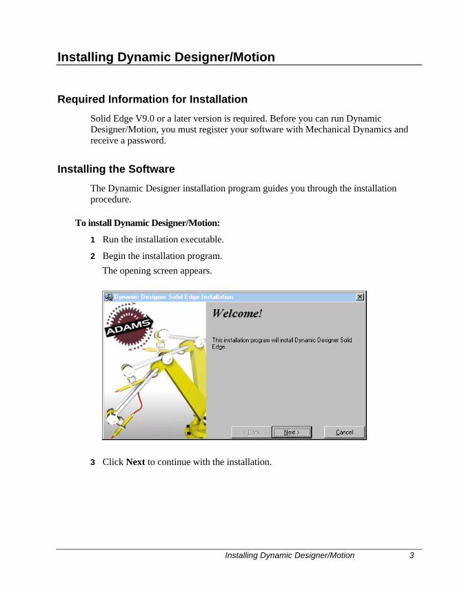
1 Run the installation executable.
2 Begin the installation program.
The opening screen appears.
3 Click Next to continue with the installation.
4 Installing Dynamic Designer/Motion
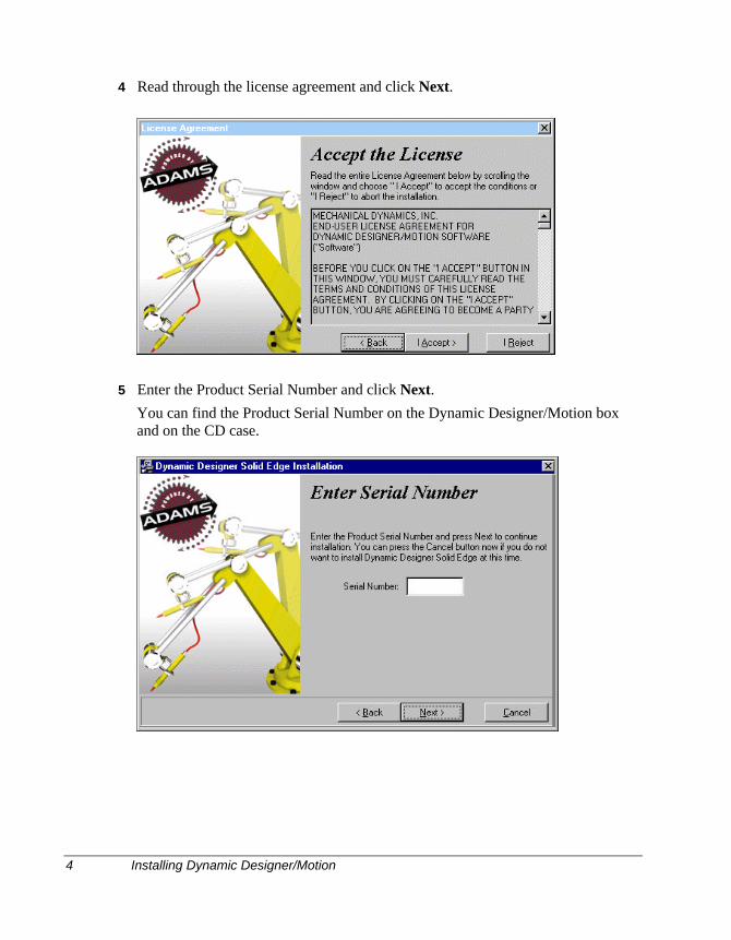
4 Read through the license agreement and click Next.
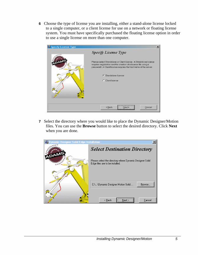
5 Enter the Product Serial Number and click Next.
You can find the Product Serial Number on the Dynamic Designer/Motion boxand on the CD case.
Installing Dynamic Designer/Motion 5
6 Choose the type of license you are installing, either a stand-alone license lockedto a single computer, or a client license for use on a network or floating licensesystem. You must have specifically purchased the floating license option in orderto use a single license on more than one computer.
7 Select the directory where you would like to place the Dynamic Designer/Motionfiles. You can use the Browse button to select the desired directory. Click Nextwhen you are done.
6 Installing Dynamic Designer/Motion
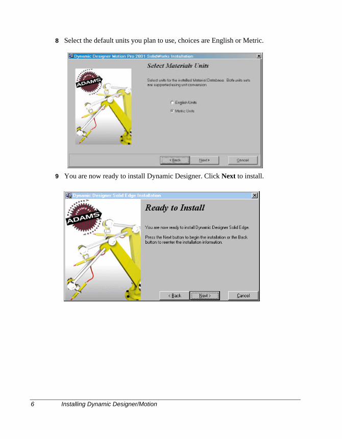
8 Select the default units you plan to use, choices are English or Metric.
9 You are now ready to install Dynamic Designer. Click Next to install.
Installing Dynamic Designer/Motion 7
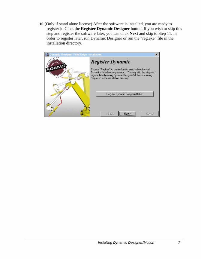
10 (Only if stand alone license) After the software is installed, you are ready toregister it. Click the Register Dynamic Designer button. If you wish to skip thisstep and register the software later, you can click Next and skip to Step 11. Inorder to register later, run Dynamic Designer or run the “reg.exe” file in theinstallation directory.
8 Installing Dynamic Designer/Motion
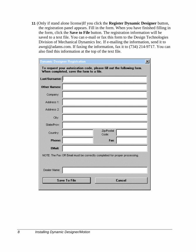
11 (Only if stand alone license)If you click the Register Dynamic Designer button,the registration panel appears. Fill in the form. When you have finished filling inthe form, click the Save to File button. The registration information will besaved to a text file. You can e-mail or fax this form to the Design TechnologiesDivision of Mechanical Dynamics Inc. If e-mailing the information, send it [email protected]. If faxing the information, fax it to (734) 214-9717. You canalso find this information at the top of the text file.
Installing Dynamic Designer/Motion 9
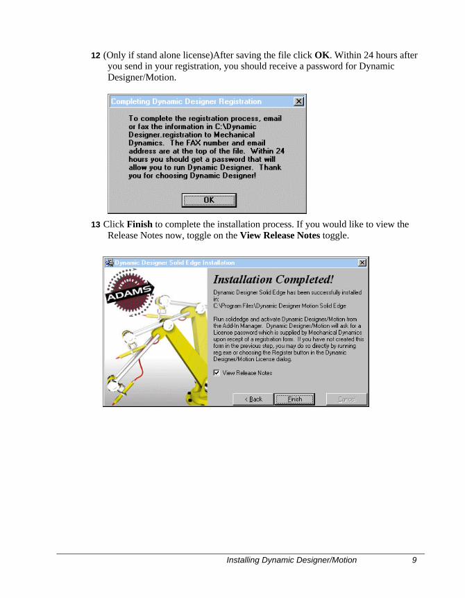
12 (Only if stand alone license)After saving the file click OK. Within 24 hours afteryou send in your registration, you should receive a password for DynamicDesigner/Motion.
13 Click Finish to complete the installation process. If you would like to view theRelease Notes now, toggle on the View Release Notes toggle.
10 Licensing
Licensing
Stand Alone License
Before Dynamic Designer Motion can be used, a license code must be entered. Youshould have already filled in the registration information and sent it to MechanicalDynamics to get your license code.
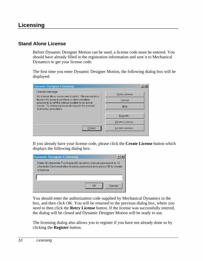
The first time you enter Dynamic Designer Motion, the following dialog box will bedisplayed:
If you already have your license code, please click the Create License button whichdisplays the following dialog box:
You should enter the authorization code supplied by Mechanical Dynamics in thebox, and then click OK. You will be returned to the previous dialog box, where youneed to then click the Retry License button. If the license was successfully entered,the dialog will be closed and Dynamic Designer Motion will be ready to use.
The licensing dialog also allows you to register if you have not already done so byclicking the Register button.
Licensing 11
If you have an existing license that is not located in the default location, you can usethat license by clicking the Locate License button and select the file that contains theDynamic Designer Motion license file.
If you have problems with licensing and want to contact your dealer or MechanicalDynamics to assist in resolving the problems, please click the Details button andrecord all of the information displayed. Your dealer or Mechanical Dynamics supportpersonnel will need this information to diagnose your licensing problem.
Floating License
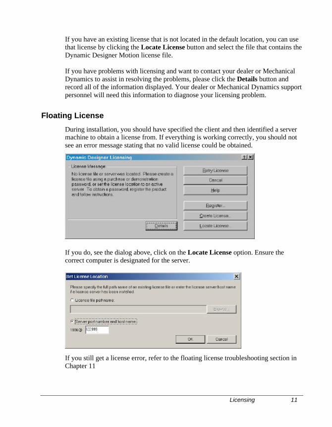
During installation, you should have specified the client and then identified a servermachine to obtain a license from. If everything is working correctly, you should notsee an error message stating that no valid license could be obtained.
If you do, see the dialog above, click on the Locate License option. Ensure thecorrect computer is designated for the server.
If you still get a license error, refer to the floating license troubleshooting section inChapter 11

12 Product Structure
Product Structure
This manual is intended to describe the operation of both the Dynamic DesignerMotion and the Dynamic Designer Motion/Professional product. Capabilities that arepresent in Dynamic Designer Motion Professional and not in Dynamic DesignerMotion will be marked as such.
User Interface 13
User Interface
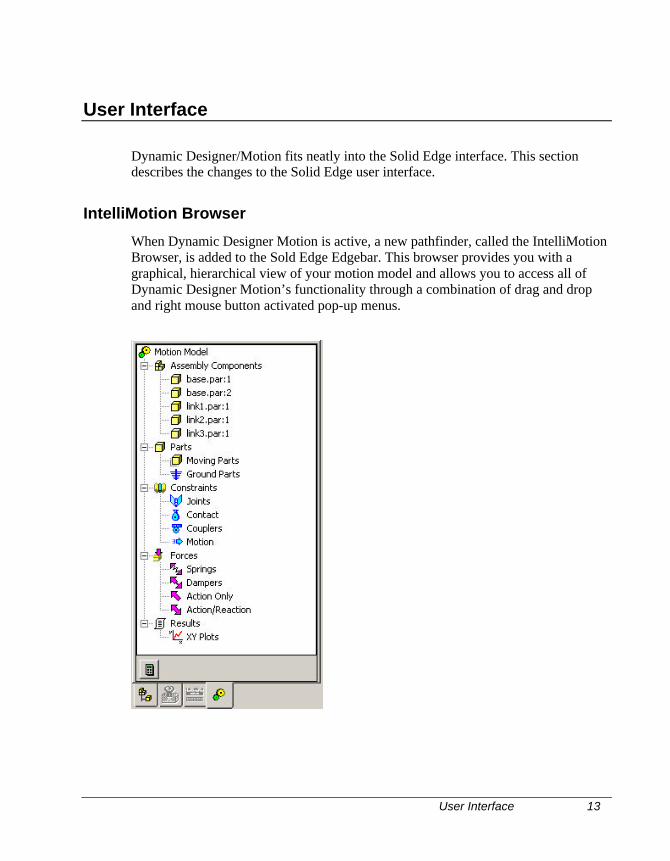
Dynamic Designer/Motion fits neatly into the Solid Edge interface. This sectiondescribes the changes to the Solid Edge user interface.
IntelliMotion Browser
When Dynamic Designer Motion is active, a new pathfinder, called the IntelliMotionBrowser, is added to the Sold Edge Edgebar. This browser provides you with agraphical, hierarchical view of your motion model and allows you to access all ofDynamic Designer Motion’s functionality through a combination of drag and dropand right mouse button activated pop-up menus.
14 User Interface
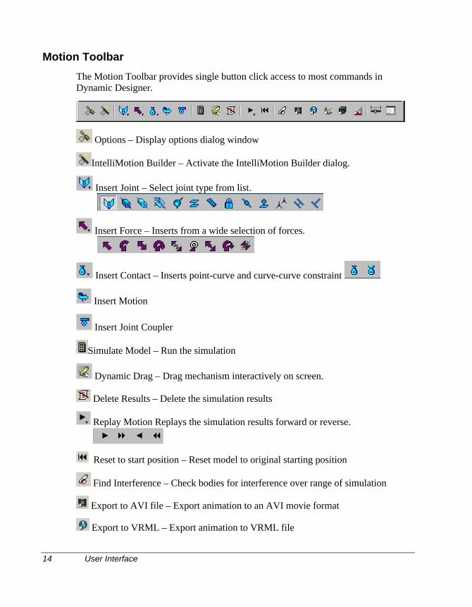
Motion Toolbar
The Motion Toolbar provides single button click access to most commands inDynamic Designer.
Options – Display options dialog window
IntelliMotion Builder – Activate the IntelliMotion Builder dialog.
Insert Joint – Select joint type from list.
Insert Force – Inserts from a wide selection of forces.
Insert Contact – Inserts point-curve and curve-curve constraint
Insert Motion
Insert Joint Coupler
Simulate Model – Run the simulation
Dynamic Drag – Drag mechanism interactively on screen.
Delete Results – Delete the simulation results
Replay Motion Replays the simulation results forward or reverse.
Reset to start position – Reset model to original starting position
Find Interference – Check bodies for interference over range of simulation
Export to AVI file – Export animation to an AVI movie format
Export to VRML – Export animation to VRML file
Steps in Defining and Simulating a Mechanism 15
Export to FEA – Export motion based loads for stress analysis
Export to ADAMS – Export mechanism and geometry to ADAMS products
Show Simulation Panel – Display Simulation panel for replaying motion
Show Message Window - Display messages from simulation
For further information, refer to the specific areas in the manual on how to use thesefeatures.
Steps in Defining and Simulating a Mechanism
To create a mechanism, you first indicate to Dynamic Designer Motion which of thecomponents in your assembly participate in the motion model. You do this bydragging and dropping the components in the IntelliMotion Browser. Any assemblymates that exist between the components are automatically converted to DynamicDesigner Motion joints. You can then add other motion specific elements to yourmotion model resulting in a completely defined mechanism. You then submit themechanism to the embedded ADAMS simulation engine, so it can determine how themechanism will perform and behave. You can view the results of the simulation asan animation showing the motion of your mechanism or as numeric output. The stepsin defining and analyzing a mechanism are explained below.
1 Review your product concept -
Identify the components of interest, how they are connected, and what drives themovement of the components. Determine which characteristics of the product youwant to understand by running a system-level simulation.
2 Indicate which components from your assembly will participate in the motionmodel. -
Using drag and drop techniques in the IntelliMotion Browser, indicate whichassembly components are moving parts, which are ground parts, and whichcomponents may be rigidly attached to other components. Dynamic DesignerMotion will create motion joints from an assembly mates that exist betweencomponents in the motion model. Additionally, you may manually add motionjoints when a suitable assembly mate does not exist.
3 Apply motion to the constraints in your mechanism -
16 Steps in Defining and Simulating a Mechanism
You can attach motion inputs to a joint’s free degrees of freedom. A motion caninput either rotational or translational motion as a function of time. For example,the function, TIME * 360d, defines a motion driver that rotates one body onecomplete revolution (360 degrees) with respect to another body per unit of time.
4 Add applied loads (optional, Dynamic Designer/Motion only) -
Applied loads are external forces and torques that act on your mechanism.
5 Run a simulation of the mechanism -
With a click of a button, you invoke the embedded simulation engine, theADAMS/Solver that solves the equations of motion for your mechanism. Thesolver calculates the displacement, velocity, acceleration, and reaction forcesacting on each moving part in the mechanism.
6 Review the simulation results -
You can view an animation of the simulation. Animations help you understand thebehavior of your mechanism and help you communicate that information toothers.
You can also view the numeric output from the simulation to understand variouscharacteristics of your mechanism. For example, Dynamic Designer/Motionreports the loads for each joint and motion. Joint loads can be used to set up loadcases for the structural analysis of any component in your mechanism.
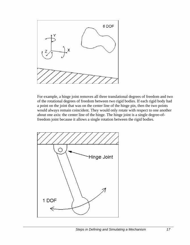
About Degrees of Freedom
A rigid body free in space has six degrees of freedom: three translational and threerotational. It can move along its X, Y, and Z axes and rotate about its X, Y, and Zaxes. When you add a constraint, such as a hinge joint, between two rigid bodies, youremove degrees of freedom between the bodies, causing them to remain positionedwith respect to one another regardless of any motion or force in the mechanism. Theconstraints in Dynamic Designer remove various numbers and combinations ofdegrees of freedom.
Steps in Defining and Simulating a Mechanism 17
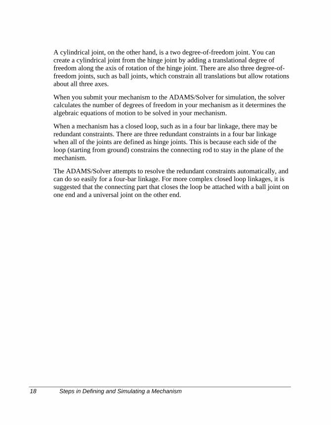
For example, a hinge joint removes all three translational degrees of freedom and twoof the rotational degrees of freedom between two rigid bodies. If each rigid body hada point on the joint that was on the center line of the hinge pin, then the two pointswould always remain coincident. They would only rotate with respect to one anotherabout one axis: the center line of the hinge. The hinge joint is a single degree-of-freedom joint because it allows a single rotation between the rigid bodies.
18 Steps in Defining and Simulating a Mechanism
A cylindrical joint, on the other hand, is a two degree-of-freedom joint. You cancreate a cylindrical joint from the hinge joint by adding a translational degree offreedom along the axis of rotation of the hinge joint. There are also three degree-of-freedom joints, such as ball joints, which constrain all translations but allow rotationsabout all three axes.
When you submit your mechanism to the ADAMS/Solver for simulation, the solvercalculates the number of degrees of freedom in your mechanism as it determines thealgebraic equations of motion to be solved in your mechanism.
When a mechanism has a closed loop, such as in a four bar linkage, there may beredundant constraints. There are three redundant constraints in a four bar linkagewhen all of the joints are defined as hinge joints. This is because each side of theloop (starting from ground) constrains the connecting rod to stay in the plane of themechanism.
The ADAMS/Solver attempts to resolve the redundant constraints automatically, andcan do so easily for a four-bar linkage. For more complex closed loop linkages, it issuggested that the connecting part that closes the loop be attached with a ball joint onone end and a universal joint on the other end.
Modeling Procedure 19
With Dynamic Designer/Motion, you can use your assemblies to define workingprototypes of your product concept. Joints and forces can be quickly and easily addedto your solid model. This chapter describes ADAMS entities and how you createthem with Dynamic Designer.
This chapter covers the following topics:
q Mechanism Modeling Procedure
q Motion Parts
q Constraints
q Motion Drivers
q Rigid Bodies
q Forces
q Manipulating mechanism entities
Modeling Procedure
The second step in simulating your mechanical system involves defining theassembly and creating the mechanism. See “Steps in Defining and Simulating aMechanism” on page 15 for the procedure on how to simulate your mechanicalsystem. To create a mechanism, use the following procedure. The mechanism entitiesdiscussed in the procedure below are covered in more detail later in the chapter.
To create a mechanism:
1 Indicate which components from your Solid Edge assembly will participate in themotion model by using drag and drop in the IntelliMotion Browser.
2 Creating Mechanisms
20 Automatically Create Parts and Joints
2 Define any additional joints in your mechanical system by selecting theappropriate joint from the Joint menu, opening the Insert Joint dialog box, andthen selecting the Solid Edge components that you wish to constrain.
3 Define motion drivers to drive joints in your mechanical system. Not all jointswill have motions applied to them.
4 Define any gravitational forces, springs, dampers, or other loads acting on yourmechanism. (optional step)
Automatically Create Parts and Joints
An optional way to create your mechanism is to let Dynamic Designer Motion domost of the work for you as you build your Solid Edge assembly model.
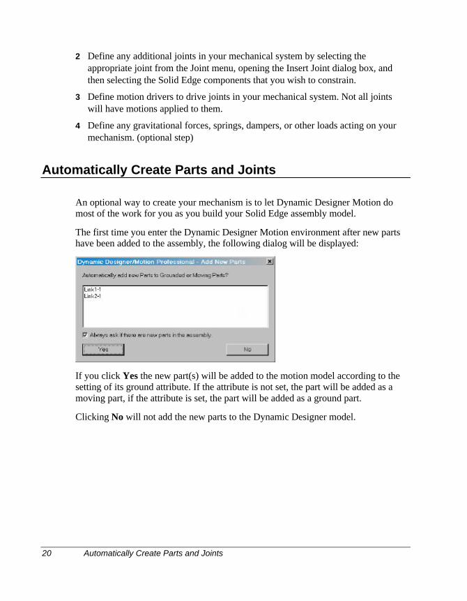
The first time you enter the Dynamic Designer Motion environment after new partshave been added to the assembly, the following dialog will be displayed:
If you click Yes the new part(s) will be added to the motion model according to thesetting of its ground attribute. If the attribute is not set, the part will be added as amoving part, if the attribute is set, the part will be added as a ground part.
Clicking No will not add the new parts to the Dynamic Designer model.
Automatically Create Parts and Joints 21
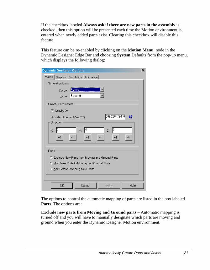
If the checkbox labeled Always ask if there are new parts in the assembly ischecked, then this option will be presented each time the Motion environment isentered when newly added parts exist. Clearing this checkbox will disable thisfeature.
This feature can be re-enabled by clicking on the Motion Menu node in theDynamic Designer Edge Bar and choosing System Defaults from the pop-up menu,which displays the following dialog:
The options to control the automatic mapping of parts are listed in the box labeledParts. The options are:
Exclude new parts from Moving and Ground parts – Automatic mapping isturned off and you will have to manually designate which parts are moving andground when you enter the Dynamic Designer Motion environment.
22 Motion Parts
Map new parts to Moving and Ground parts – Every new part added to the SolidEdge assembly is automatically mapped to a Dynamic Designer Motion part the nexttime the Motion environment is entered. The choice of moving or ground part isdetermined by the setting of the part’s ground attribute in Solid Edge.
Ask before mapping parts - The dialog box described above will be displayed eachtime the Motion environment is entered and new parts exist in the Solid Edgeassembly.
Motion Parts
The first step in creating a mechanism is to indicate which components from yourSolid Edge assembly model will participate in the motion model. This isaccomplished by using either drag-and-drop, or right mouse button activated pop-upmenus from the IntelliMotion Browser.
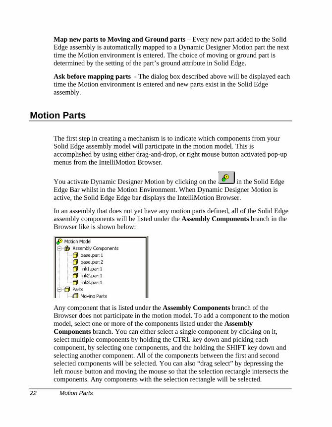
You activate Dynamic Designer Motion by clicking on the in the Solid EdgeEdge Bar whilst in the Motion Environment. When Dynamic Designer Motion isactive, the Solid Edge Edge bar displays the IntelliMotion Browser.
In an assembly that does not yet have any motion parts defined, all of the Solid Edgeassembly components will be listed under the Assembly Components branch in theBrowser like is shown below:
Any component that is listed under the Assembly Components branch of theBrowser does not participate in the motion model. To add a component to the motionmodel, select one or more of the components listed under the AssemblyComponents branch. You can either select a single component by clicking on it,select multiple components by holding the CTRL key down and picking eachcomponent, by selecting one components, and the holding the SHIFT key down andselecting another component. All of the components between the first and secondselected components will be selected. You can also “drag select” by depressing theleft mouse button and moving the mouse so that the selection rectangle intersects thecomponents. Any components with the selection rectangle will be selected.
Motion Parts 23
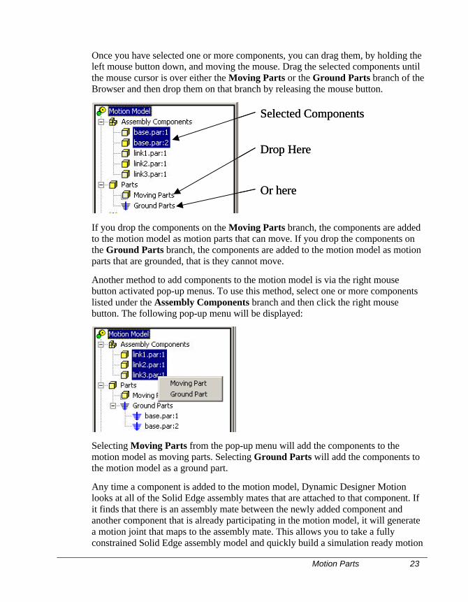
Once you have selected one or more components, you can drag them, by holding theleft mouse button down, and moving the mouse. Drag the selected components untilthe mouse cursor is over either the Moving Parts or the Ground Parts branch of theBrowser and then drop them on that branch by releasing the mouse button.
Selected Components
Drop Here
Or here
Selected Components
Drop Here
Or here
If you drop the components on the Moving Parts branch, the components are addedto the motion model as motion parts that can move. If you drop the components onthe Ground Parts branch, the components are added to the motion model as motionparts that are grounded, that is they cannot move.
Another method to add components to the motion model is via the right mousebutton activated pop-up menus. To use this method, select one or more componentslisted under the Assembly Components branch and then click the right mousebutton. The following pop-up menu will be displayed:
Selecting Moving Parts from the pop-up menu will add the components to themotion model as moving parts. Selecting Ground Parts will add the components tothe motion model as a ground part.
Any time a component is added to the motion model, Dynamic Designer Motionlooks at all of the Solid Edge assembly mates that are attached to that component. Ifit finds that there is an assembly mate between the newly added component andanother component that is already participating in the motion model, it will generatea motion joint that maps to the assembly mate. This allows you to take a fullyconstrained Solid Edge assembly model and quickly build a simulation ready motion
24 Rigidly Attached Parts
model just by indicating which components from the assembly participate in themotion model.
Rigidly Attached Parts
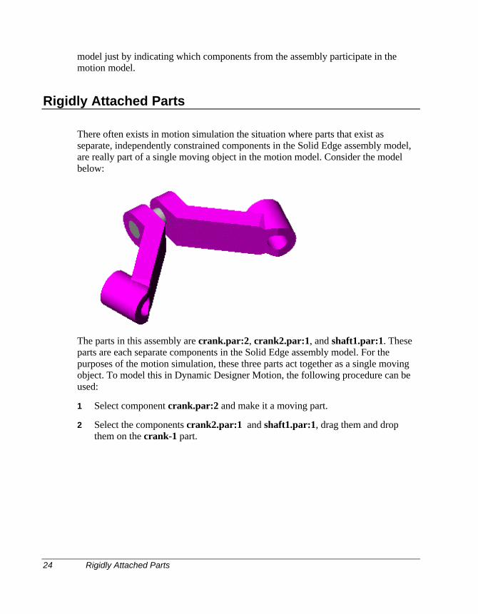
There often exists in motion simulation the situation where parts that exist asseparate, independently constrained components in the Solid Edge assembly model,are really part of a single moving object in the motion model. Consider the modelbelow:
The parts in this assembly are crank.par:2, crank2.par:1, and shaft1.par:1. Theseparts are each separate components in the Solid Edge assembly model. For thepurposes of the motion simulation, these three parts act together as a single movingobject. To model this in Dynamic Designer Motion, the following procedure can beused:
1 Select component crank.par:2 and make it a moving part.
2 Select the components crank2.par:1 and shaft1.par:1, drag them and dropthem on the crank-1 part.
Constraints 25
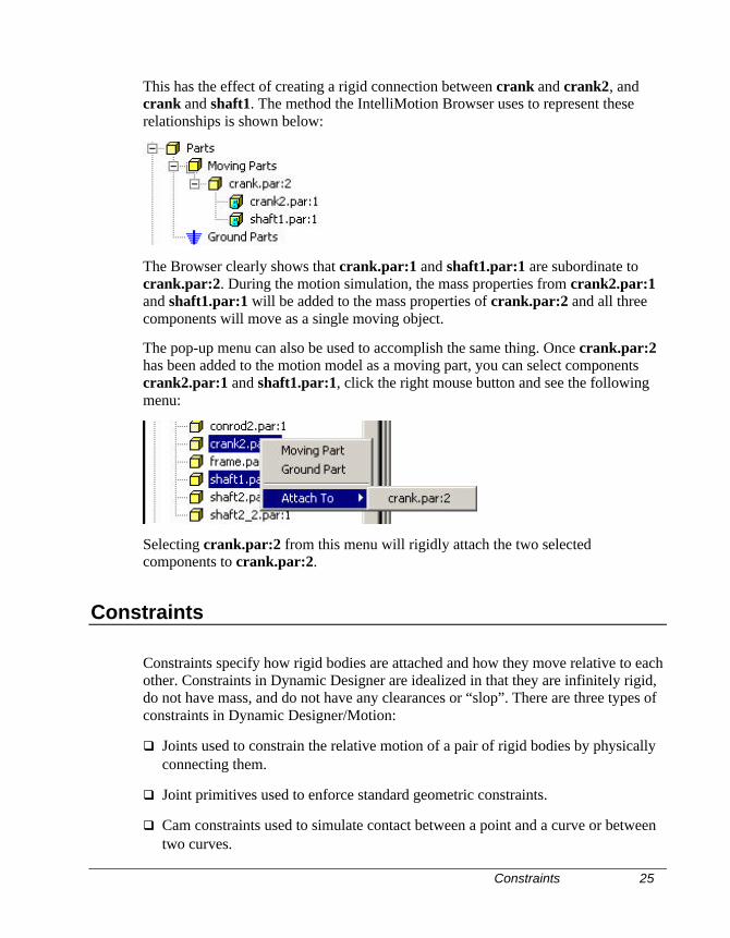
This has the effect of creating a rigid connection between crank and crank2, andcrank and shaft1. The method the IntelliMotion Browser uses to represent theserelationships is shown below:
The Browser clearly shows that crank.par:1 and shaft1.par:1 are subordinate tocrank.par:2. During the motion simulation, the mass properties from crank2.par:1and shaft1.par:1 will be added to the mass properties of crank.par:2 and all threecomponents will move as a single moving object.
The pop-up menu can also be used to accomplish the same thing. Once crank.par:2has been added to the motion model as a moving part, you can select componentscrank2.par:1 and shaft1.par:1, click the right mouse button and see the followingmenu:
Selecting crank.par:2 from this menu will rigidly attach the two selectedcomponents to crank.par:2.
Constraints
Constraints specify how rigid bodies are attached and how they move relative to eachother. Constraints in Dynamic Designer are idealized in that they are infinitely rigid,do not have mass, and do not have any clearances or “slop”. There are three types ofconstraints in Dynamic Designer/Motion:
q Joints used to constrain the relative motion of a pair of rigid bodies by physicallyconnecting them.
q Joint primitives used to enforce standard geometric constraints.
q Cam constraints used to simulate contact between a point and a curve or betweentwo curves.
26 Constraints
Constraints and applied loads are associative with the geometry that is used to definethem. In other words, if a joint origin is defined by an endpoint of an edge and if thatendpoint is moved because of a modification made to the geometry, then the jointwill move with that endpoint.
Joint and Joint Primitives are generated automatically from Solid Edge assemblymates. However, any joint or joint primitive may be added manually to the motionmodel using the techniques described below.Note: The associativity between Solid Edge and Dynamic Designer/Motion is
unidirectional. Any changes to the Dynamic Designer constraints or appliedloads will not be transferred to the Solid Edge geometry.
Understanding Joints
A joint is used to constrain the relative motion of a pair of rigid bodies by physicallyconnecting them.Note: A rigid body acts and moves as a single unit. Solid Edge components
automatically become rigid bodies in Dynamic Designer.
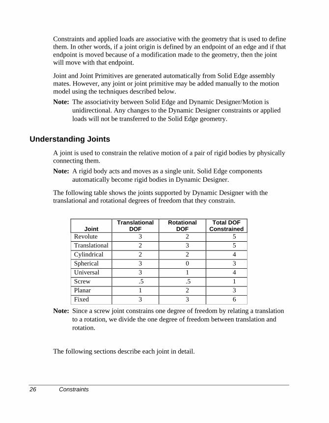
The following table shows the joints supported by Dynamic Designer with thetranslational and rotational degrees of freedom that they constrain.
JointTranslational
DOFRotational
DOFTotal DOF
ConstrainedRevolute 3 2 5Translational 2 3 5Cylindrical 2 2 4Spherical 3 0 3Universal 3 1 4Screw .5 .5 1Planar 1 2 3Fixed 3 3 6
Note: Since a screw joint constrains one degree of freedom by relating a translationto a rotation, we divide the one degree of freedom between translation androtation.
The following sections describe each joint in detail.
Revolute Joint 27
Revolute Joint
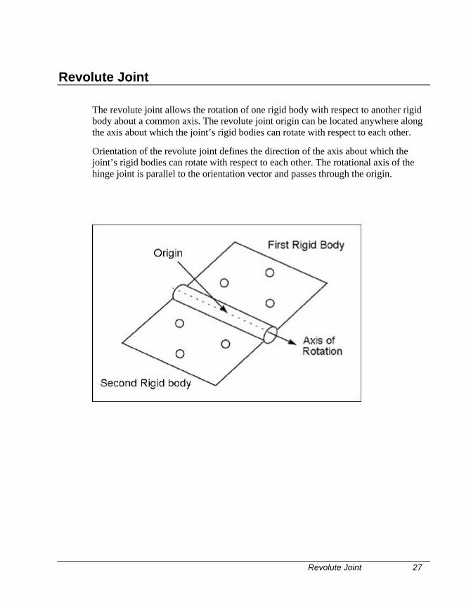
The revolute joint allows the rotation of one rigid body with respect to another rigidbody about a common axis. The revolute joint origin can be located anywhere alongthe axis about which the joint’s rigid bodies can rotate with respect to each other.
Orientation of the revolute joint defines the direction of the axis about which thejoint’s rigid bodies can rotate with respect to each other. The rotational axis of thehinge joint is parallel to the orientation vector and passes through the origin.
28 Translational Joint
Translational Joint
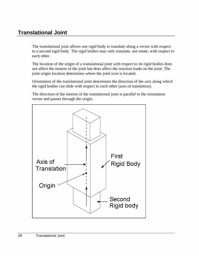
The translational joint allows one rigid body to translate along a vector with respectto a second rigid body. The rigid bodies may only translate, not rotate, with respect toeach other.
The location of the origin of a translational joint with respect to its rigid bodies doesnot affect the motion of the joint but does affect the reaction loads on the joint. Thejoint origin location determines where the joint icon is located.
Orientation of the translational joint determines the direction of the axis along whichthe rigid bodies can slide with respect to each other (axis of translation).
The direction of the motion of the translational joint is parallel to the orientationvector and passes through the origin.
Cylindrical Joint 29
Cylindrical Joint
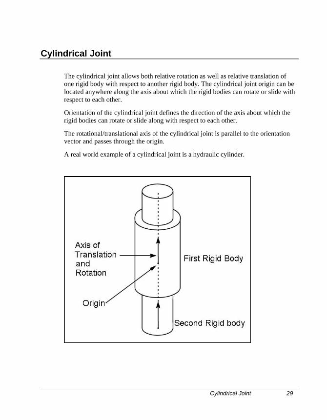
The cylindrical joint allows both relative rotation as well as relative translation ofone rigid body with respect to another rigid body. The cylindrical joint origin can belocated anywhere along the axis about which the rigid bodies can rotate or slide withrespect to each other.
Orientation of the cylindrical joint defines the direction of the axis about which therigid bodies can rotate or slide along with respect to each other.
The rotational/translational axis of the cylindrical joint is parallel to the orientationvector and passes through the origin.
A real world example of a cylindrical joint is a hydraulic cylinder.
30 Spherical Joint
Spherical Joint
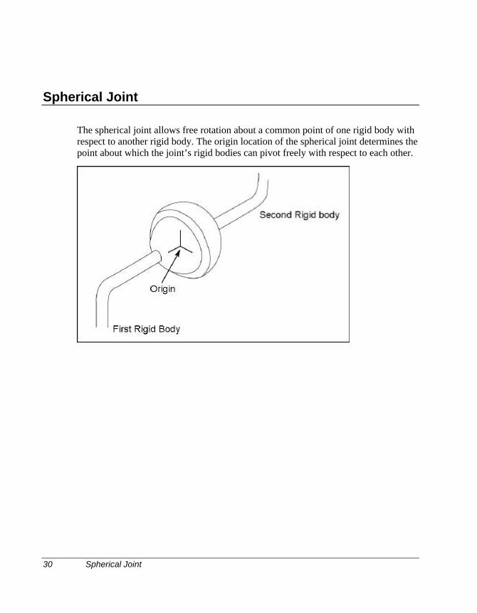
The spherical joint allows free rotation about a common point of one rigid body withrespect to another rigid body. The origin location of the spherical joint determines thepoint about which the joint’s rigid bodies can pivot freely with respect to each other.
Universal Joint 31
Universal Joint
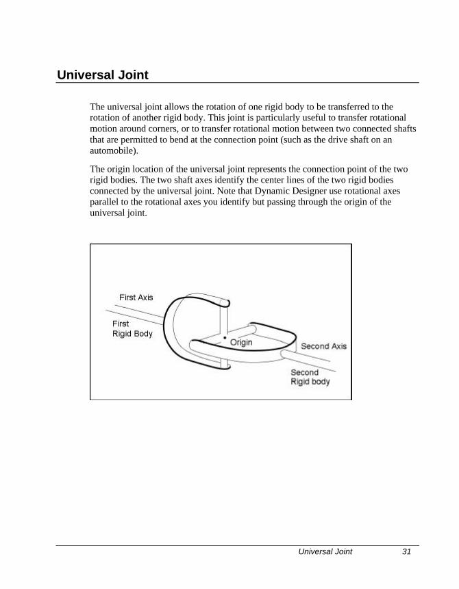
The universal joint allows the rotation of one rigid body to be transferred to therotation of another rigid body. This joint is particularly useful to transfer rotationalmotion around corners, or to transfer rotational motion between two connected shaftsthat are permitted to bend at the connection point (such as the drive shaft on anautomobile).
The origin location of the universal joint represents the connection point of the tworigid bodies. The two shaft axes identify the center lines of the two rigid bodiesconnected by the universal joint. Note that Dynamic Designer use rotational axesparallel to the rotational axes you identify but passing through the origin of theuniversal joint.
32 Screw Joint
Screw Joint
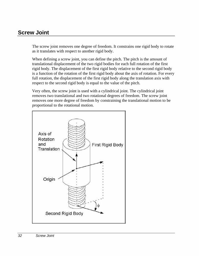
The screw joint removes one degree of freedom. It constrains one rigid body to rotateas it translates with respect to another rigid body.
When defining a screw joint, you can define the pitch. The pitch is the amount oftranslational displacement of the two rigid bodies for each full rotation of the firstrigid body. The displacement of the first rigid body relative to the second rigid bodyis a function of the rotation of the first rigid body about the axis of rotation. For everyfull rotation, the displacement of the first rigid body along the translation axis withrespect to the second rigid body is equal to the value of the pitch.
Very often, the screw joint is used with a cylindrical joint. The cylindrical jointremoves two translational and two rotational degrees of freedom. The screw jointremoves one more degree of freedom by constraining the translational motion to beproportional to the rotational motion.
Planar Joint 33
Planar Joint
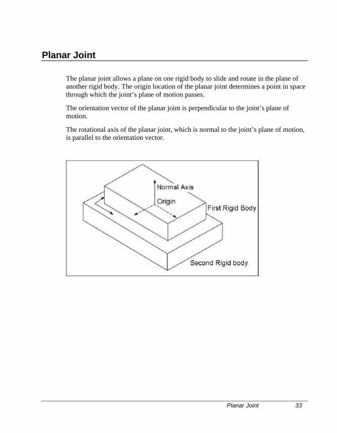
The planar joint allows a plane on one rigid body to slide and rotate in the plane ofanother rigid body. The origin location of the planar joint determines a point in spacethrough which the joint’s plane of motion passes.
The orientation vector of the planar joint is perpendicular to the joint’s plane ofmotion.
The rotational axis of the planar joint, which is normal to the joint’s plane of motion,is parallel to the orientation vector.
34 Fixed Joint
Fixed Joint
The fixed joint locks two rigid bodies together so they may not move with respect toeach other.
For a fixed joint, the origin location and orientation of the joint does not effect theoutcome of the simulation. We recommend that you place the joint origin at alocation where the graphic icon is easily visible.
A real world example of a fixed joint is a weld that holds two parts together.
Joint Friction 35
Joint Friction
Joint Friction is only available in Motion Professional.
Revolute, Cylindrical, Translational, Spherical, Universal, and Planar joints all support theapplication of friction. When friction effects are enabled for these joint types, a force isinduced that opposes the motion of the joint and is a function of the reaction forces acting onthe joint.
The Dynamic Designer Motion joint friction model uses a combination of dimensionalinformation assigned to a joint and a coefficient of friction that may be entered directly, orthat may be obtained automatically from the materials database.
36 Joint Friction
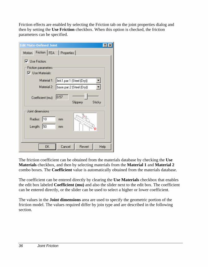
Friction effects are enabled by selecting the Friction tab on the joint properties dialog andthen by setting the Use Friction checkbox. When this option is checked, the frictionparameters can be specified.
The friction coefficient can be obtained from the materials database by checking the UseMaterials checkbox, and then by selecting materials from the Material 1 and Material 2combo boxes. The Coefficient value is automatically obtained from the materials database.
The coefficient can be entered directly by clearing the Use Materials checkbox that enablesthe edit box labeled Coefficient (mu) and also the slider next to the edit box. The coefficientcan be entered directly, or the slider can be used to select a higher or lower coefficient.
The values in the Joint dimensions area are used to specify the geometric portion of thefriction model. The values required differ by join type and are described in the followingsection.
Joint Friction 37
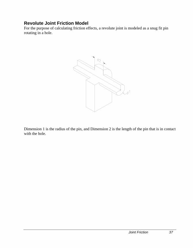
Revolute Joint Friction ModelFor the purpose of calculating friction effects, a revolute joint is modeled as a snug fit pinrotating in a hole.
Dimension 1 is the radius of the pin, and Dimension 2 is the length of the pin that is in contactwith the hole.
38 Joint Friction
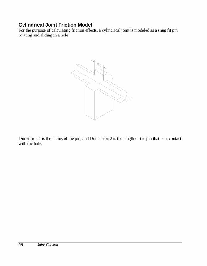
Cylindrical Joint Friction ModelFor the purpose of calculating friction effects, a cylindrical joint is modeled as a snug fit pinrotating and sliding in a hole.
Dimension 1 is the radius of the pin, and Dimension 2 is the length of the pin that is in contactwith the hole.
Joint Friction 39
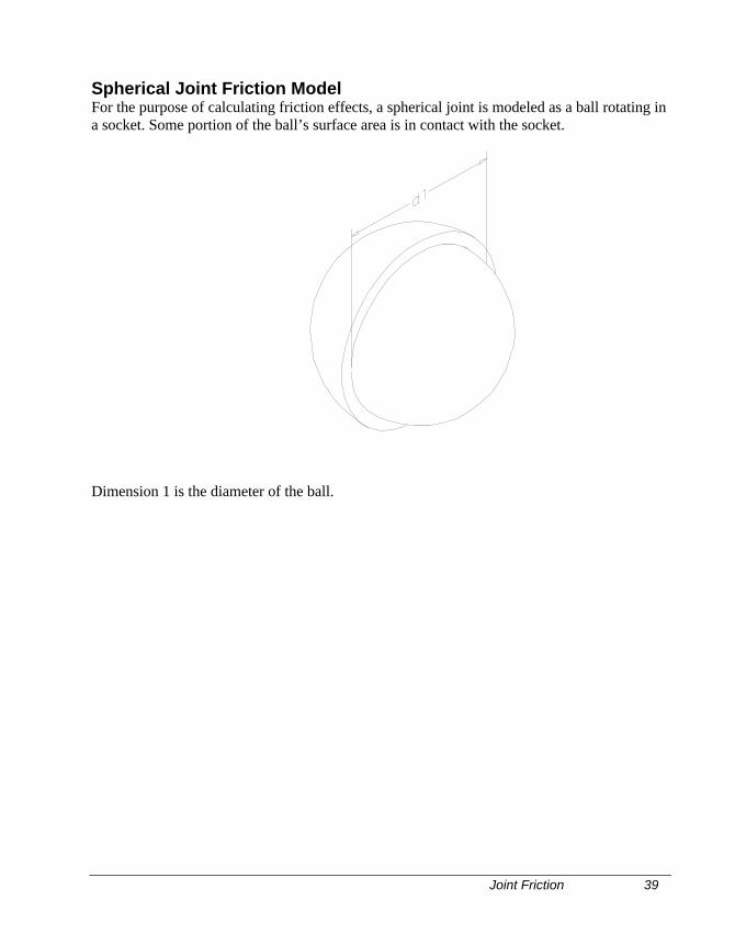
Spherical Joint Friction ModelFor the purpose of calculating friction effects, a spherical joint is modeled as a ball rotating ina socket. Some portion of the ball’s surface area is in contact with the socket.
Dimension 1 is the diameter of the ball.
40 Joint Friction
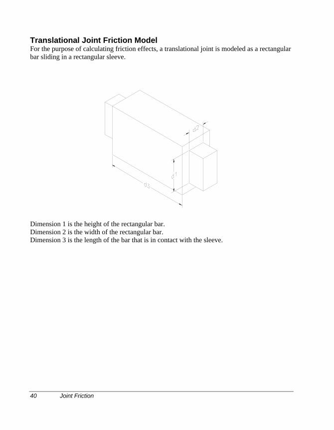
Translational Joint Friction ModelFor the purpose of calculating friction effects, a translational joint is modeled as a rectangularbar sliding in a rectangular sleeve.
Dimension 1 is the height of the rectangular bar.Dimension 2 is the width of the rectangular bar.Dimension 3 is the length of the bar that is in contact with the sleeve.
Joint Friction 41
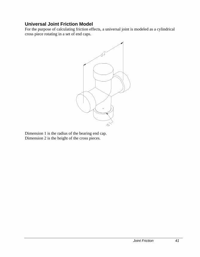
Universal Joint Friction ModelFor the purpose of calculating friction effects, a universal joint is modeled as a cylindricalcross piece rotating in a set of end caps.
Dimension 1 is the radius of the bearing end cap.Dimension 2 is the height of the cross pieces.
42 Joint Friction
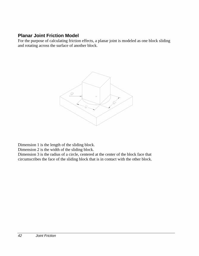
Planar Joint Friction ModelFor the purpose of calculating friction effects, a planar joint is modeled as one block slidingand rotating across the surface of another block.
Dimension 1 is the length of the sliding block.Dimension 2 is the width of the sliding block.Dimension 3 is the radius of a circle, centered at the center of the block face thatcircumscribes the face of the sliding block that is in contact with the other block.
Joint Friction 43
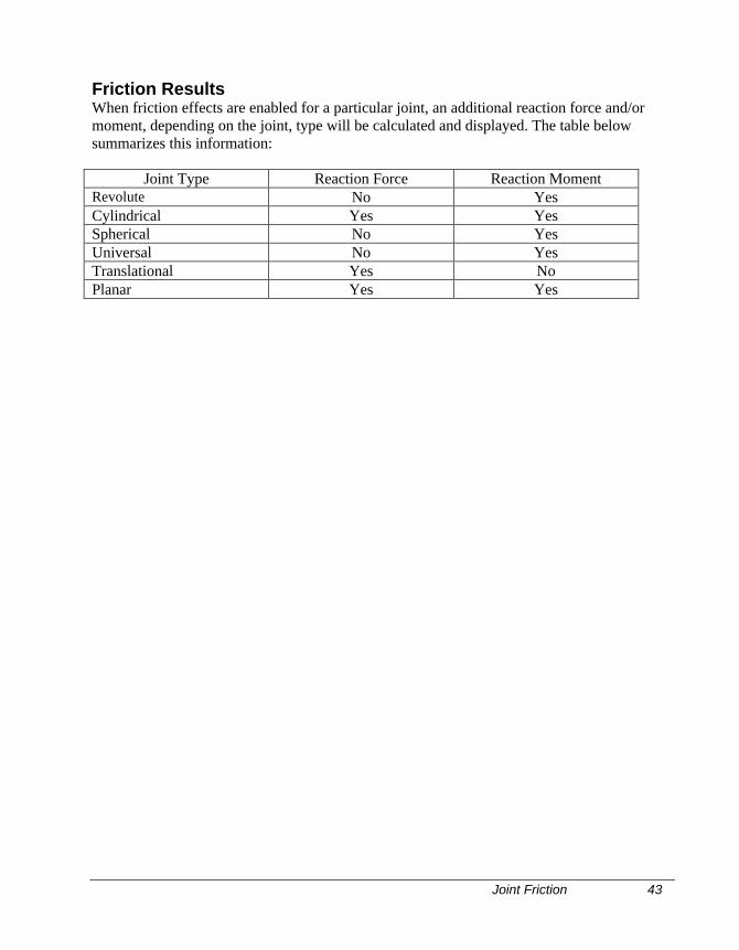
Friction ResultsWhen friction effects are enabled for a particular joint, an additional reaction force and/ormoment, depending on the joint, type will be calculated and displayed. The table belowsummarizes this information:
Joint Type Reaction Force Reaction MomentRevolute No YesCylindrical Yes YesSpherical No YesUniversal No YesTranslational Yes NoPlanar Yes Yes
44 Understanding Joint Primitives
Understanding Joint Primitives
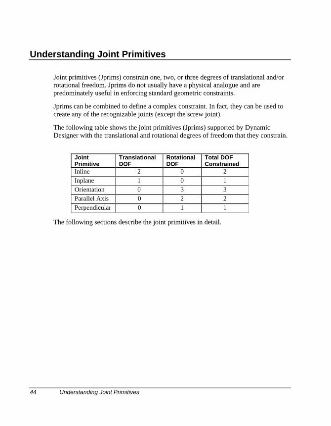
Joint primitives (Jprims) constrain one, two, or three degrees of translational and/orrotational freedom. Jprims do not usually have a physical analogue and arepredominately useful in enforcing standard geometric constraints.
Jprims can be combined to define a complex constraint. In fact, they can be used tocreate any of the recognizable joints (except the screw joint).
The following table shows the joint primitives (Jprims) supported by DynamicDesigner with the translational and rotational degrees of freedom that they constrain.
JointPrimitive
TranslationalDOF
RotationalDOF
Total DOFConstrained
Inline 2 0 2Inplane 1 0 1Orientation 0 3 3Parallel Axis 0 2 2Perpendicular 0 1 1
The following sections describe the joint primitives in detail.
Inline JPrim 45
Inline JPrim
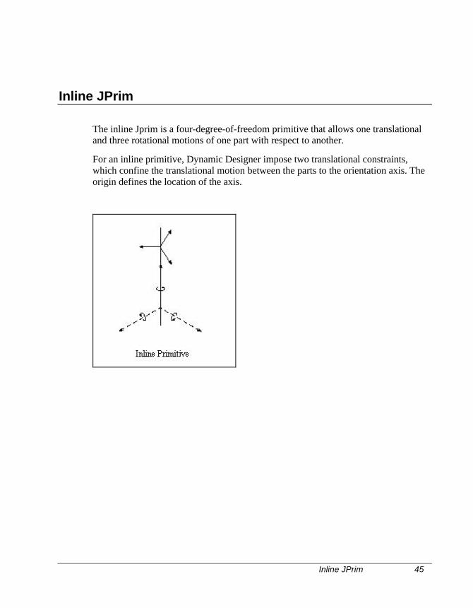
The inline Jprim is a four-degree-of-freedom primitive that allows one translationaland three rotational motions of one part with respect to another.
For an inline primitive, Dynamic Designer impose two translational constraints,which confine the translational motion between the parts to the orientation axis. Theorigin defines the location of the axis.
46 Inplane JPrim
Inplane JPrim
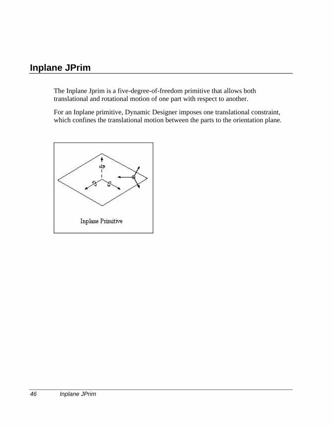
The Inplane Jprim is a five-degree-of-freedom primitive that allows bothtranslational and rotational motion of one part with respect to another.
For an Inplane primitive, Dynamic Designer imposes one translational constraint,which confines the translational motion between the parts to the orientation plane.
Orientation JPrim 47
Orientation JPrim
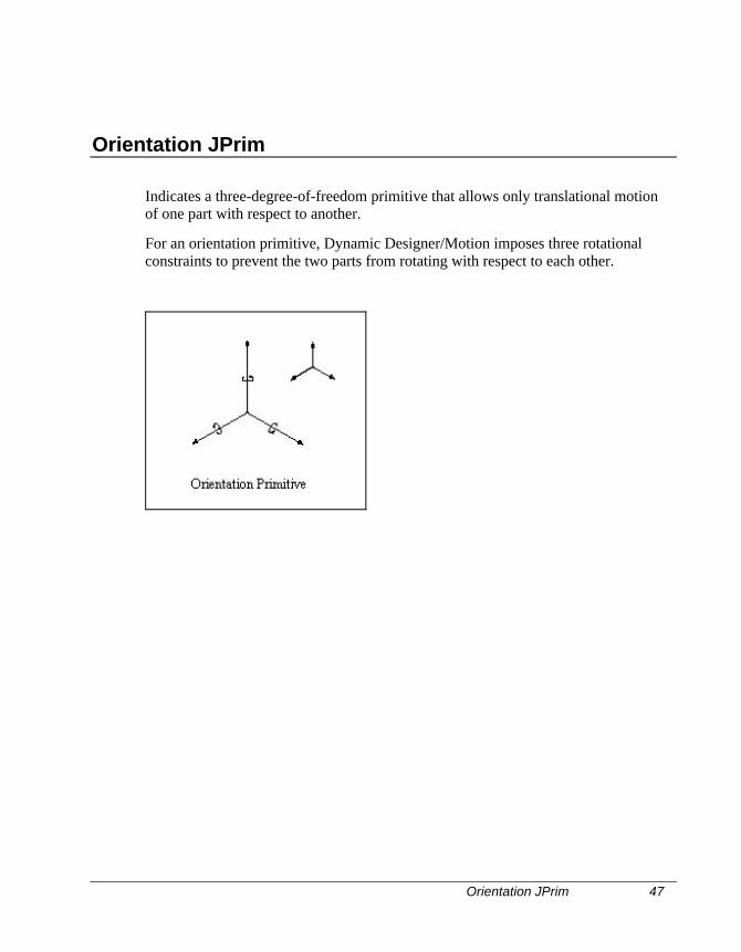
Indicates a three-degree-of-freedom primitive that allows only translational motionof one part with respect to another.
For an orientation primitive, Dynamic Designer/Motion imposes three rotationalconstraints to prevent the two parts from rotating with respect to each other.
48 Parallel Axes JPrim
Parallel Axes JPrim
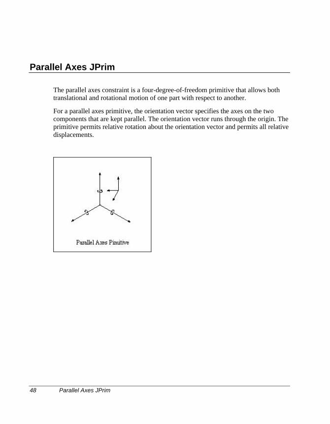
The parallel axes constraint is a four-degree-of-freedom primitive that allows bothtranslational and rotational motion of one part with respect to another.
For a parallel axes primitive, the orientation vector specifies the axes on the twocomponents that are kept parallel. The orientation vector runs through the origin. Theprimitive permits relative rotation about the orientation vector and permits all relativedisplacements.
Perpendicular JPrim 49
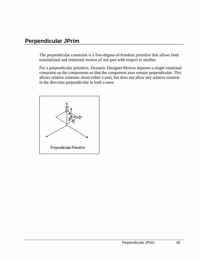
Perpendicular JPrim
The perpendicular constraint is a five-degree-of-freedom primitive that allows bothtranslational and rotational motion of one part with respect to another.
For a perpendicular primitive, Dynamic Designer/Motion imposes a single rotationalconstraint on the components so that the component axes remain perpendicular. Thisallows relative rotations about either z-axis, but does not allow any relative rotationin the direction perpendicular to both z-axes.
50 Understanding Motions
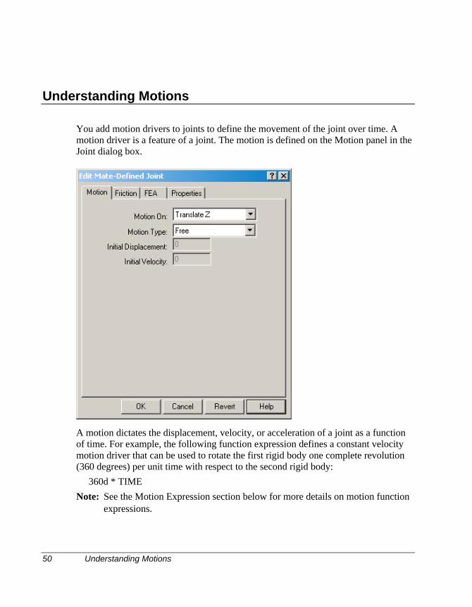
Understanding Motions
You add motion drivers to joints to define the movement of the joint over time. Amotion driver is a feature of a joint. The motion is defined on the Motion panel in theJoint dialog box.
A motion dictates the displacement, velocity, or acceleration of a joint as a functionof time. For example, the following function expression defines a constant velocitymotion driver that can be used to rotate the first rigid body one complete revolution(360 degrees) per unit time with respect to the second rigid body:
360d * TIMENote: See the Motion Expression section below for more details on motion function
expressions.
Understanding Motions 51
The motion driver supplies the force required to make the joint satisfy the definedmotion. This force is available as an output at each motion driver in DynamicDesigner/Motion. This output can be used to properly size a motor or actuator.
Degrees of Freedom
In the DOF field on the Motion panel, you can select the degree of freedom to whichthe motion is applied. The degrees of freedom can be either rotational ortranslational. For example, hinge joints have one rotational degree of freedom. Youmay apply only one rotational motion to a hinge joint. Planar joints have twotranslational and one rotational degree of freedom. Therefore, you can apply twotranslational motions and one rotational motion to a planar joint. You can apply amotion to any degree of freedom on a joint.
Motion Type
A motion driver can define either the joint displacement, velocity, or acceleration. Bydefault, the motion driver type is set to “free”, meaning that the joint is free to moveas driven by the rest of the mechanism. You can set the motion type in the InsertJoint dialog box on the Motion panel. The simplest motions to define are the constantdisplacement, constant velocity, or constant acceleration motions:
q Constant Displacement - Placing a constant value in the Motion Expression fieldwhen the motion type is set to Displacement creates a constant displacementmotion. A constant displacement motion holds the joint in a fixed position. Therigid bodies that the joint connects do not move relative to each other duringsimulation. The effect is very much like using a fixed joint to constrain the tworigid bodies. The advantage of constraining two parts with a constantdisplacement motion is that the motion can be adjusted to different positions.Constraining two rigid bodies with a fixed joint, however, is computationallymore efficient.
q Constant Velocity - Placing a constant value in the Motion Expression fieldwhen the motion type is set to Velocity creates a constant velocity motion, whichmoves the joint with the required force to produce a constant velocity.
q Constant Acceleration - Placing a constant value in the Motion Expression fieldwhen the motion type is set to Acceleration creates a constant accelerationmotion. This motion moves the joint with the required force to produce a constantacceleration.
52 Motion Expression
Motion Expression
A motion function specifies the exact displacement, velocity, or acceleration appliedto a joint as a function of time. There are four pre-defined functions supported.Additionally a general expression capability is available that allows any ADAMSfunction to be specified. When the Motion Type is set to something other than Free,a combo box labeled Function is displayed the allows the choice of function. Thefour predefined function are described below.
q Constant Function - The Constant Function creates a function expression thatmoves the joint displacement, velocity, or acceleration in a constant manner. Onevalue needs to be specified.
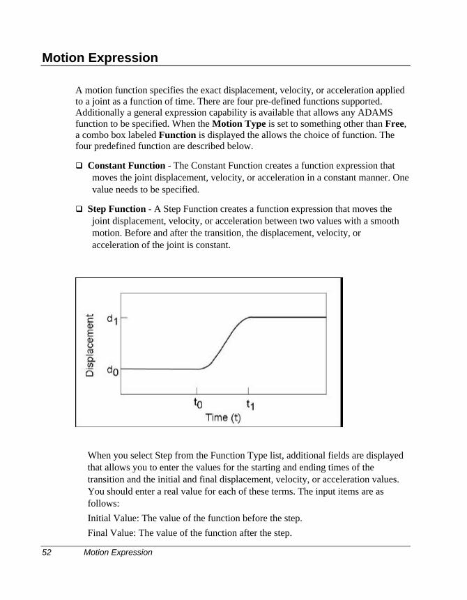
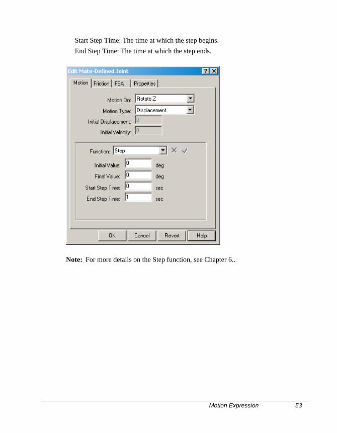
q Step Function - A Step Function creates a function expression that moves thejoint displacement, velocity, or acceleration between two values with a smoothmotion. Before and after the transition, the displacement, velocity, oracceleration of the joint is constant.
When you select Step from the Function Type list, additional fields are displayedthat allows you to enter the values for the starting and ending times of thetransition and the initial and final displacement, velocity, or acceleration values.You should enter a real value for each of these terms. The input items are asfollows:Initial Value: The value of the function before the step.Final Value: The value of the function after the step.
Motion Expression 53
Start Step Time: The time at which the step begins.End Step Time: The time at which the step ends.
Note: For more details on the Step function, see Chapter 6..
54 Motion Expression
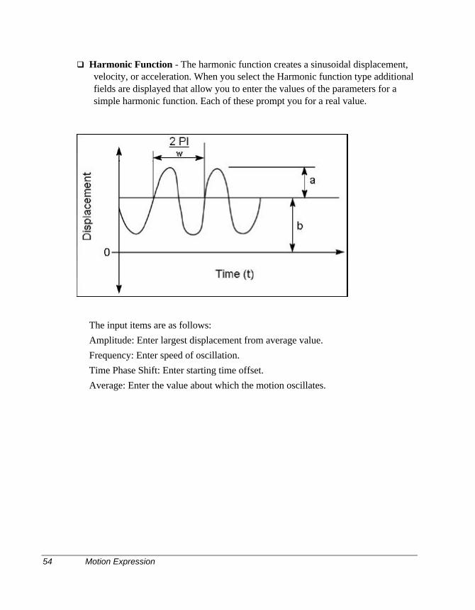
q Harmonic Function - The harmonic function creates a sinusoidal displacement,velocity, or acceleration. When you select the Harmonic function type additionalfields are displayed that allow you to enter the values of the parameters for asimple harmonic function. Each of these prompt you for a real value.
The input items are as follows:Amplitude: Enter largest displacement from average value.Frequency: Enter speed of oscillation.Time Phase Shift: Enter starting time offset.Average: Enter the value about which the motion oscillates.
Motion Expression 55
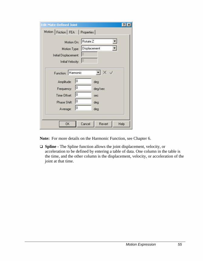
Note: For more details on the Harmonic Function, see Chapter 6.
q Spline - The Spline function allows the joint displacement, velocity, oracceleration to be defined by entering a table of data. One column in the table isthe time, and the other column is the displacement, velocity, or acceleration of thejoint at that time.
56 Motion Expression
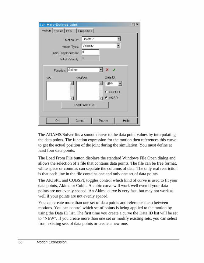
The ADAMS/Solver fits a smooth curve to the data point values by interpolatingthe data points. The function expression for the motion then references this curveto get the actual position of the joint during the simulation. You must define atleast four data points.
The Load From File button displays the standard Windows File Open dialog andallows the selection of a file that contains data points. The file can be free format,white space or commas can separate the columns of data. The only real restrictionis that each line in the file contains one and only one set of data points.The AKISPL and CUBSPL toggles control which kind of curve is used to fit yourdata points, Akima or Cubic. A cubic curve will work well even if your datapoints are not evenly spaced. An Akima curve is very fast, but may not work aswell if your points are not evenly spaced.You can create more than one set of data points and reference them betweenmotions. You can control which set of points is being applied to the motion byusing the Data ID list. The first time you create a curve the Data ID list will be setto “NEW”. If you create more than one set or modify existing sets, you can selectfrom existing sets of data points or create a new one.
Creating Joints, Joint Primitives, and Motions 57
Other Function Expressions
ADAMS functions are only available in Motion Professional.
You can also enter the text for other ADAMS function expressions in the MotionExpression field. The function expression of a motion driver must be a function oftime. If you make your motion expression a function of displacements, forces, or anyother variables in the system, the ADAMS/Solver issues an error message and stopsexecution.
If you enter an incorrect expression, Dynamic Designer/Motion will issue an errormessage indicating that your expression is incorrect. You can not close the InsertJoint dialog box until you correct the expression.
See Chapter 6 for a list of functions that are supported in Dynamic Designer/Motion.
Creating Joints, Joint Primitives, and Motions
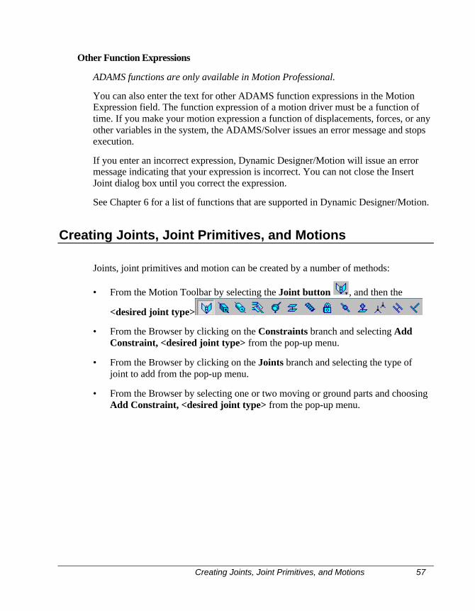
Joints, joint primitives and motion can be created by a number of methods:
• From the Motion Toolbar by selecting the Joint button , and then the
<desired joint type>
• From the Browser by clicking on the Constraints branch and selecting AddConstraint, <desired joint type> from the pop-up menu.
• From the Browser by clicking on the Joints branch and selecting the type ofjoint to add from the pop-up menu.
• From the Browser by selecting one or two moving or ground parts and choosingAdd Constraint, <desired joint type> from the pop-up menu.
58 Creating Joints, Joint Primitives, and Motions
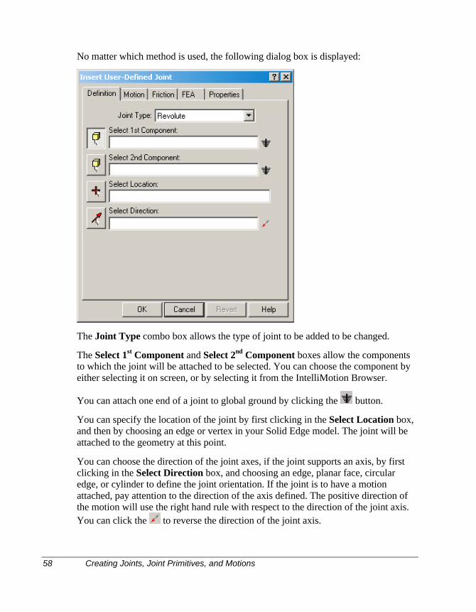
No matter which method is used, the following dialog box is displayed:
The Joint Type combo box allows the type of joint to be added to be changed.
The Select 1st Component and Select 2nd Component boxes allow the componentsto which the joint will be attached to be selected. You can choose the component byeither selecting it on screen, or by selecting it from the IntelliMotion Browser.
You can attach one end of a joint to global ground by clicking the button.
You can specify the location of the joint by first clicking in the Select Location box,and then by choosing an edge or vertex in your Solid Edge model. The joint will beattached to the geometry at this point.
You can choose the direction of the joint axes, if the joint supports an axis, by firstclicking in the Select Direction box, and choosing an edge, planar face, circularedge, or cylinder to define the joint orientation. If the joint is to have a motionattached, pay attention to the direction of the axis defined. The positive direction ofthe motion will use the right hand rule with respect to the direction of the joint axis.You can click the to reverse the direction of the joint axis.
Creating Joints, Joint Primitives, and Motions 59
To locate and orient joints, you can take full advantage of the existing Solid Edgegeometry. When you are selecting the components to which the joint is connected,you can select geometry features that will automatically define the origin andorientation of the joint. The first geometry feature selected may define both the originand orientation. If it does not, the second geometry feature selected may define eitheror both the origin and the orientation. If geometry features are not selected or if theorigin or the orientation is not defined by the selection of the components, then youmust separately define the origin and/or the orientation. The table below lists whichgeometry features automatically define the origin and orientation.
Geometry Feature Joint Origin at: Orientation/direction:Linear Edge Midpoint of edge Vector parallel to
edgeVertex Point <Is not set>Planar face <Is not set> Normal to faceCircular edge Center of circle Normal to faceCylinder <Is not set> Centerline of
cylinder
When selecting the components or geometry when defining joints or forces, you caneasily replace the geometry or components after you select them. You can replacethem as you create the joint or force or when you edit them.
Once all of the information for the joint has been defined, you can click the OKbutton to actually create the joint. Once OK has been clicked, the joint dialog will beclosed.
60 Creating Joints, Joint Primitives, and Motions
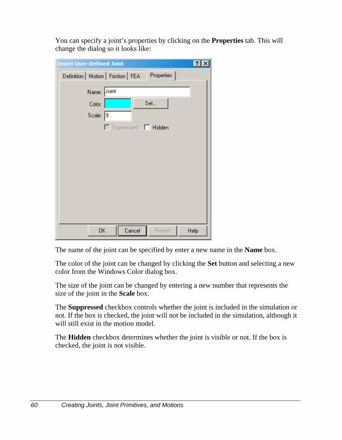
You can specify a joint’s properties by clicking on the Properties tab. This willchange the dialog so it looks like:
The name of the joint can be specified by enter a new name in the Name box.
The color of the joint can be changed by clicking the Set button and selecting a newcolor from the Windows Color dialog box.
The size of the joint can be changed by entering a new number that represents thesize of the joint in the Scale box.
The Suppressed checkbox controls whether the joint is included in the simulation ornot. If the box is checked, the joint will not be included in the simulation, although itwill still exist in the motion model.
The Hidden checkbox determines whether the joint is visible or not. If the box ischecked, the joint is not visible.
Creating Joints, Joint Primitives, and Motions 61
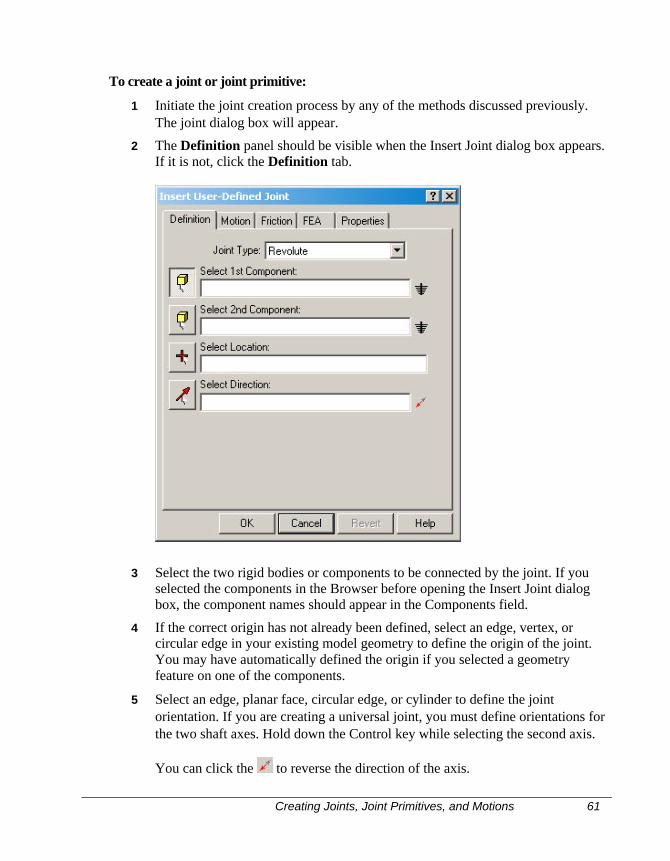
To create a joint or joint primitive:
1 Initiate the joint creation process by any of the methods discussed previously.The joint dialog box will appear.
2 The Definition panel should be visible when the Insert Joint dialog box appears.If it is not, click the Definition tab.
3 Select the two rigid bodies or components to be connected by the joint. If youselected the components in the Browser before opening the Insert Joint dialogbox, the component names should appear in the Components field.
4 If the correct origin has not already been defined, select an edge, vertex, orcircular edge in your existing model geometry to define the origin of the joint.You may have automatically defined the origin if you selected a geometryfeature on one of the components.
5 Select an edge, planar face, circular edge, or cylinder to define the jointorientation. If you are creating a universal joint, you must define orientations forthe two shaft axes. Hold down the Control key while selecting the second axis.
You can click the to reverse the direction of the axis.
62 Creating Joints, Joint Primitives, and Motions
Once the origin and orientation have been defined, the joint icon will appear onthe screen at the joint origin with the defined orientation.
6 If you are creating a screw joint, you can also define the pitch of the joint byentering it in the box at the bottom of the Definitions page.
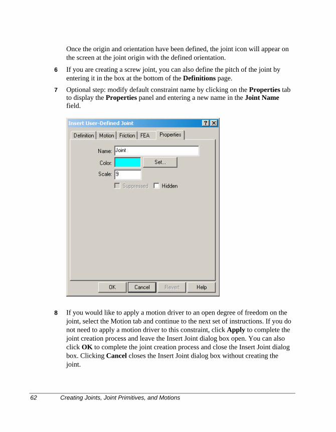
7 Optional step: modify default constraint name by clicking on the Properties tabto display the Properties panel and entering a new name in the Joint Namefield.
8 If you would like to apply a motion driver to an open degree of freedom on thejoint, select the Motion tab and continue to the next set of instructions. If you donot need to apply a motion driver to this constraint, click Apply to complete thejoint creation process and leave the Insert Joint dialog box open. You can alsoclick OK to complete the joint creation process and close the Insert Joint dialogbox. Clicking Cancel closes the Insert Joint dialog box without creating thejoint.
Creating Joints, Joint Primitives, and Motions 63
The final step in creating a joint or a joint primitive is to apply a motion or motionsto the degrees of freedom of the joint. This is an optional step since you will not needto apply motions to all joints.
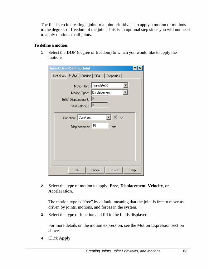
To define a motion:
1 Select the DOF (degree of freedom) to which you would like to apply themotions.
2 Select the type of motion to apply: Free, Displacement, Velocity, orAcceleration.
The motion type is “free” by default, meaning that the joint is free to move asdriven by joints, motions, and forces in the system.
3 Select the type of function and fill in the fields displayed.
For more details on the motion expression, see the Motion Expression sectionabove.
4 Click Apply
64 Understanding Contact Constraints
Understanding Contact Constraints
Dynamic Designer/Motion supports the following contact constraints:
q Point-curve - restricts a point on one rigid body to lie on a curve on a second rigidbody
q Curve-curve - constrains one curve to remain in contact with a second curve.Curve-curve also supports an intermittent option that allows the two curves toseparate and rejoin. This allows 2D contact to be modeled.
q 3D Contact – Simulates two bodies colliding by detecting when they come incontact with each other and calculating and applying the forces that result fromthat collision. While not technically a constraint, 3D contact is grouped togetherwith the other contact functionality in Dynamic Designer Motion.
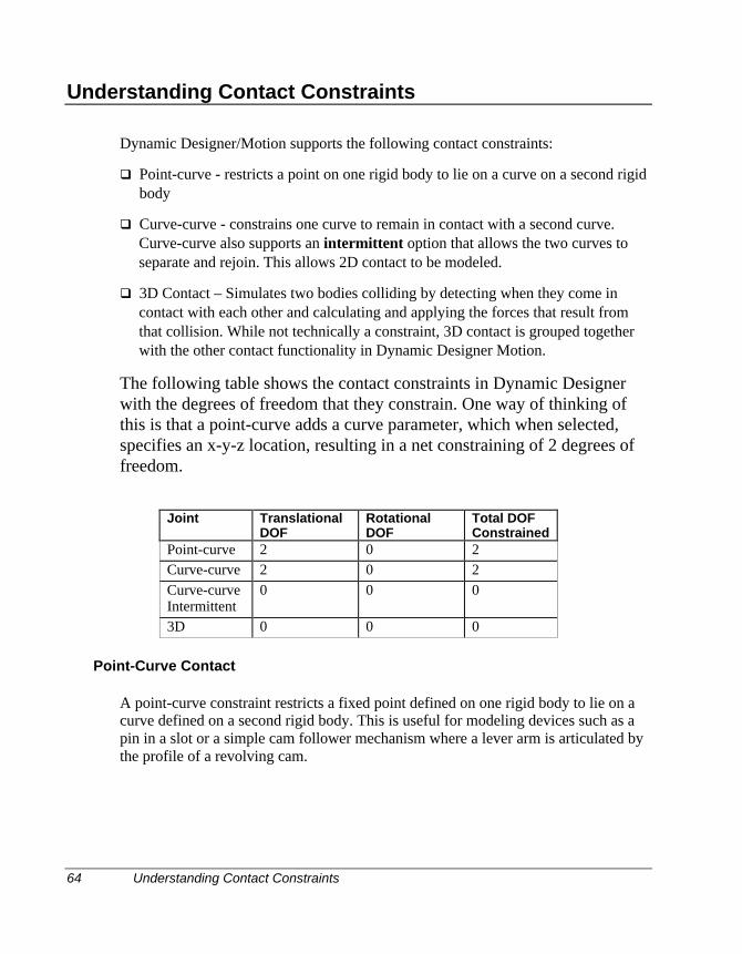
The following table shows the contact constraints in Dynamic Designerwith the degrees of freedom that they constrain. One way of thinking ofthis is that a point-curve adds a curve parameter, which when selected,specifies an x-y-z location, resulting in a net constraining of 2 degrees offreedom.
Joint TranslationalDOF
RotationalDOF
Total DOFConstrained
Point-curve 2 0 2Curve-curve 2 0 2Curve-curveIntermittent
0 0 0
3D 0 0 0
Point-Curve Contact
A point-curve constraint restricts a fixed point defined on one rigid body to lie on acurve defined on a second rigid body. This is useful for modeling devices such as apin in a slot or a simple cam follower mechanism where a lever arm is articulated bythe profile of a revolving cam.
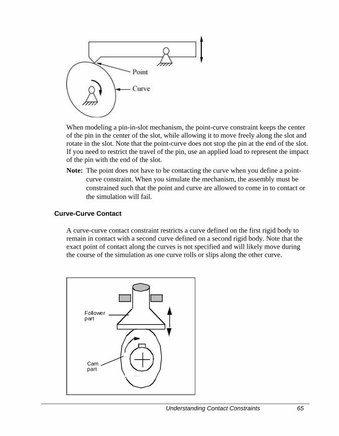
Understanding Contact Constraints 65
When modeling a pin-in-slot mechanism, the point-curve constraint keeps the centerof the pin in the center of the slot, while allowing it to move freely along the slot androtate in the slot. Note that the point-curve does not stop the pin at the end of the slot.If you need to restrict the travel of the pin, use an applied load to represent the impactof the pin with the end of the slot.Note: The point does not have to be contacting the curve when you define a point-
curve constraint. When you simulate the mechanism, the assembly must beconstrained such that the point and curve are allowed to come in to contact orthe simulation will fail.
Curve-Curve Contact
A curve-curve contact constraint restricts a curve defined on the first rigid body toremain in contact with a second curve defined on a second rigid body. Note that theexact point of contact along the curves is not specified and will likely move duringthe course of the simulation as one curve rolls or slips along the other curve.
Cam
Followerpart
part
66 Creating Contact Constraints
The curve-curve constraint is useful for modeling cams where the point of contactbetween two rigid bodies changes during the motion of the mechanism. An exampleis a valve lifter where the cam is lifting a plate-like object. The point of contactbetween the plate (flat curve) and the cam (oval curve) change depending on theposition and shape of the cam. Edges selected representing curves for the curve-curve constraint must have all points lying in the same plane. The resulting planarcurve may exist in any location and orientation in your Solid Edge assembly with thefollowing restriction.
The two curves (each defined by selected edges/datum curves) used in defining thecurve-curve constraint must lie in the same plane. It is possible to initially define thecurves such that they are not in the same plane, but Dynamic Designer will move therigid bodies during simulation to ensure that the two curves are constrained to thesame plane of motion with respect to each other.
Note: The curves do not have to be in contacting when you define a curve-curveconstraint. When you simulate the mechanism, the assembly must beconstrained such that the curves are allowed to come in to contact or thesimulation will fail.
Curve-Curve Contact with Intermittent Contact
If the Curve-Curve constraint is designated as intermittent, the curve may separateand rejoin as the dynamics of the system dictate. An intermittent curve-curveconstraint supports friction and multiple points of contact. When a curve-curveconstraint is designated as intermittent, there are additional parameters that effect thatcontact characteristics of the curve that must be specified.
3D Contact
3D contact allows the simulation of general interactions between parts as they collideand rebound. It takes into account the impact and friction portions of the collisionand calculates all the locations where the two bodies come in contact.
3D contact is more straightforward to use than 2D (Intermittent Curve/Curve)contact, but requires more computational resources than 2D contact, and in manycases will be slower to simulate.
Creating Contact Constraints
Point/Curve and Curve/Curve constraints can be created by a number of methods:
Creating Contact Constraints 67
• From the Motion Toolbar by selecting the Contact button , and thenchoosing the Point-Curve or Curve-Curve options
• From the Browser by clicking on the Constraints branch and selecting AddContact Point/Curve Contact or Add Contact Curve/Curve Contact.
• From the Browser by clicking on the Contacts branch and selecting either AddPoint/Curve Contact or Add Curve/Curve Contact from the pop-up menu.
• From the Browser by selecting one or two moving or ground parts and choosingAdd Constraint, Point/Curve Contact or Add Constraint Curve/CurveContact from the pop-up menu.
Creating Point-Curve Constraints
For the point-curve constraint, you must define a point on one rigid body and a curveon another rigid body.
To Create a Point-Curve Constraint:
1 Initiate the Point/Curve creation process by any of the methods listed above.
The Insert Point-Curve dialog box appears.
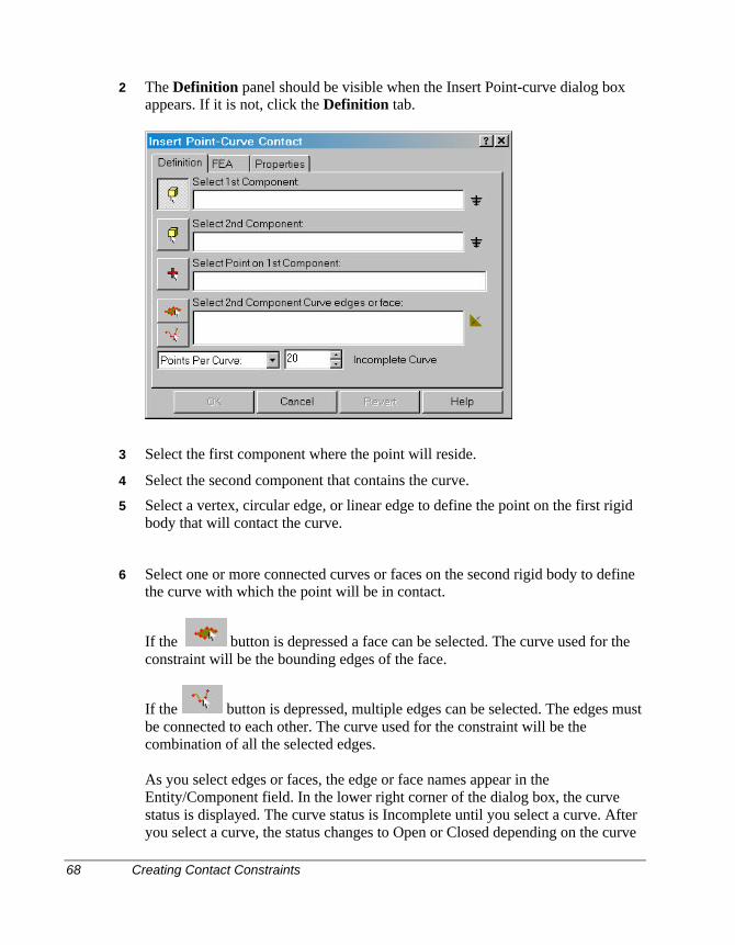
68 Creating Contact Constraints
2 The Definition panel should be visible when the Insert Point-curve dialog boxappears. If it is not, click the Definition tab.
3 Select the first component where the point will reside.
4 Select the second component that contains the curve.
5 Select a vertex, circular edge, or linear edge to define the point on the first rigidbody that will contact the curve.
6 Select one or more connected curves or faces on the second rigid body to definethe curve with which the point will be in contact.
If the button is depressed a face can be selected. The curve used for theconstraint will be the bounding edges of the face.
If the button is depressed, multiple edges can be selected. The edges mustbe connected to each other. The curve used for the constraint will be thecombination of all the selected edges.
As you select edges or faces, the edge or face names appear in theEntity/Component field. In the lower right corner of the dialog box, the curvestatus is displayed. The curve status is Incomplete until you select a curve. Afteryou select a curve, the status changes to Open or Closed depending on the curve
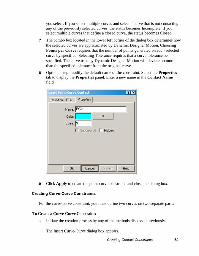
Creating Contact Constraints 69
you select. If you select multiple curves and select a curve that is not contactingany of the previously selected curves, the status becomes Incomplete. If youselect multiple curves that define a closed curve, the status becomes Closed.
7 The combo box located in the lower left corner of the dialog box determines howthe selected curves are approximated by Dynamic Designer Motion. ChoosingPoints per Curve requires that the number of points generated on each selectedcurve by specified. Selecting Tolerance requires that a curve tolerance bespecified. The curve used by Dynamic Designer Motion will deviate no morethan the specified tolerance from the original curve.
8 Optional step: modify the default name of the constraint. Select the Propertiestab to display the Properties panel. Enter a new name in the Contact Namefield.
9 Click Apply to create the point-curve constraint and close the dialog box.
Creating Curve-Curve Constraints
For the curve-curve constraint, you must define two curves on two separate parts.
To Create a Curve-Curve Constraint:
1 Initiate the creation process by any of the methods discussed previously.
The Insert Curve-Curve dialog box appears.
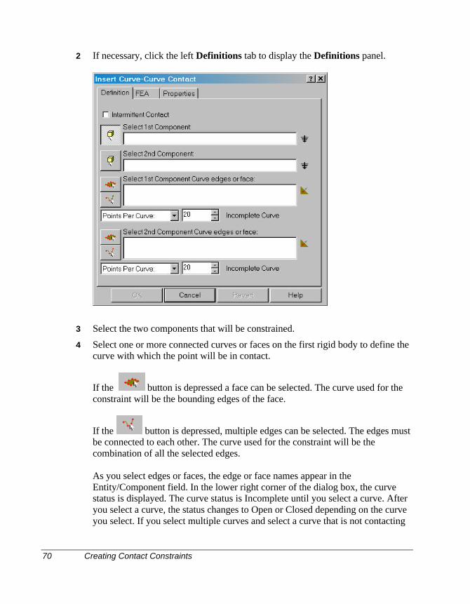
70 Creating Contact Constraints
2 If necessary, click the left Definitions tab to display the Definitions panel.
3 Select the two components that will be constrained.
4 Select one or more connected curves or faces on the first rigid body to define thecurve with which the point will be in contact.
If the button is depressed a face can be selected. The curve used for theconstraint will be the bounding edges of the face.
If the button is depressed, multiple edges can be selected. The edges mustbe connected to each other. The curve used for the constraint will be thecombination of all the selected edges.
As you select edges or faces, the edge or face names appear in theEntity/Component field. In the lower right corner of the dialog box, the curvestatus is displayed. The curve status is Incomplete until you select a curve. Afteryou select a curve, the status changes to Open or Closed depending on the curveyou select. If you select multiple curves and select a curve that is not contacting
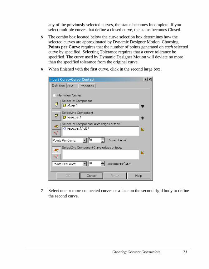
Creating Contact Constraints 71
any of the previously selected curves, the status becomes Incomplete. If youselect multiple curves that define a closed curve, the status becomes Closed.
5 The combo box located below the curve selection box determines how theselected curves are approximated by Dynamic Designer Motion. ChoosingPoints per Curve requires that the number of points generated on each selectedcurve by specified. Selecting Tolerance requires that a curve tolerance bespecified. The curve used by Dynamic Designer Motion will deviate no morethan the specified tolerance from the original curve.
6 When finished with the first curve, click in the second large box .
7 Select one or more connected curves or a face on the second rigid body to definethe second curve.
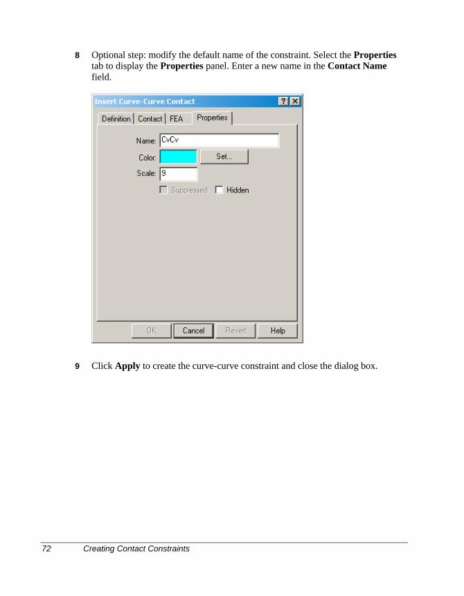
72 Creating Contact Constraints
8 Optional step: modify the default name of the constraint. Select the Propertiestab to display the Properties panel. Enter a new name in the Contact Namefield.
9 Click Apply to create the curve-curve constraint and close the dialog box.
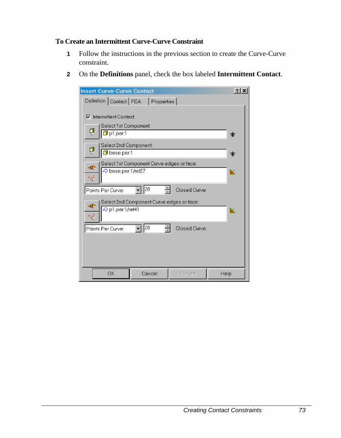
Creating Contact Constraints 73
To Create an Intermittent Curve-Curve Constraint
1 Follow the instructions in the previous section to create the Curve-Curveconstraint.
2 On the Definitions panel, check the box labeled Intermittent Contact.
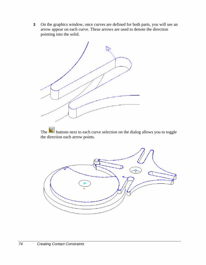
74 Creating Contact Constraints
3 On the graphics window, once curves are defined for both parts, you will see anarrow appear on each curve. These arrows are used to denote the directionpointing into the solid.
The buttons next to each curve selection on the dialog allows you to togglethe direction each arrow points.
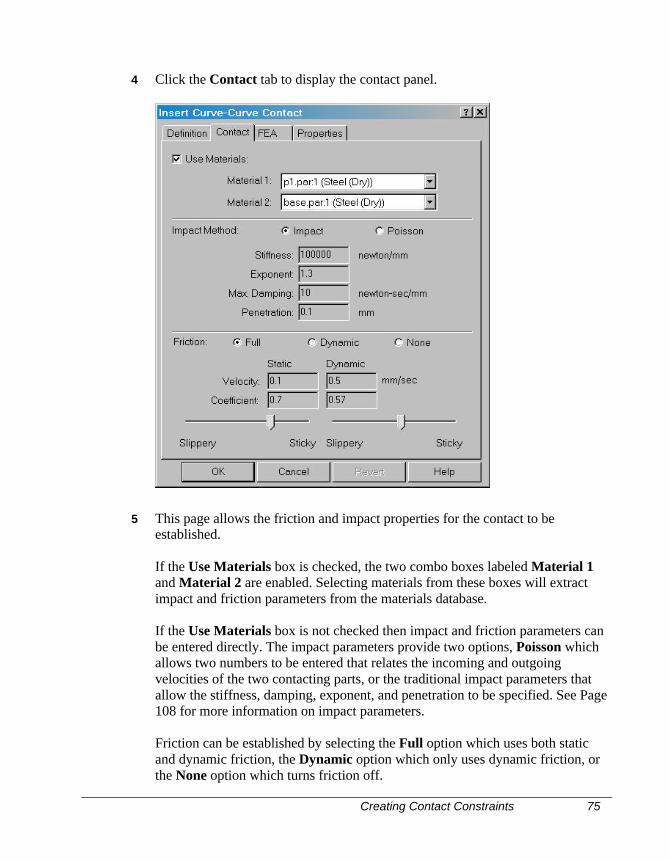
Creating Contact Constraints 75
4 Click the Contact tab to display the contact panel.
5 This page allows the friction and impact properties for the contact to beestablished.
If the Use Materials box is checked, the two combo boxes labeled Material 1and Material 2 are enabled. Selecting materials from these boxes will extractimpact and friction parameters from the materials database.
If the Use Materials box is not checked then impact and friction parameters canbe entered directly. The impact parameters provide two options, Poisson whichallows two numbers to be entered that relates the incoming and outgoingvelocities of the two contacting parts, or the traditional impact parameters thatallow the stiffness, damping, exponent, and penetration to be specified. See Page108 for more information on impact parameters.
Friction can be established by selecting the Full option which uses both staticand dynamic friction, the Dynamic option which only uses dynamic friction, orthe None option which turns friction off.
76 Creating 3D Contacts
If Full friction is selected, both the static and dynamic friction values are used. Ifthe Use Materials option is selected, the values will be obtained from thematerials database. If this option is not selected, these values can be entereddirectly.
These parameters are:
The Static Velocity is the absolute value of the velocity at which the staticcoefficient of friction starts to transition to the dynamic coefficient of friction. Atvelocities below this value, the static coefficient of friction is active.
The Dynamic Velocity is the absolute value of the velocity above which thedynamic coefficient of friction is active. For velocities between Static Velocityand Dynamic Velocity, a step function is used to transition between the staticcoefficient of friction and the dynamic coefficient of friction.
The Static Coefficient value is the static coefficient of friction and the DynamicCoefficient is the dynamic coefficient of friction. These values must be between0 and 1. The sliders can also be used to change the coefficient value.
Creating 3D Contacts
3D Contacts can be created by a number of methods:
• From the Motion menu by selecting Motion, Contact, 3D Contact…
• From the Browser by clicking on the Constraints branch and selecting AddContact 3D Contact.
• From the Browser by clicking on the Contacts branch and selecting Add 3DContact.
• From the Browser by selecting one or two moving or ground parts and choosingAdd 3D Contact from the pop-up menu.
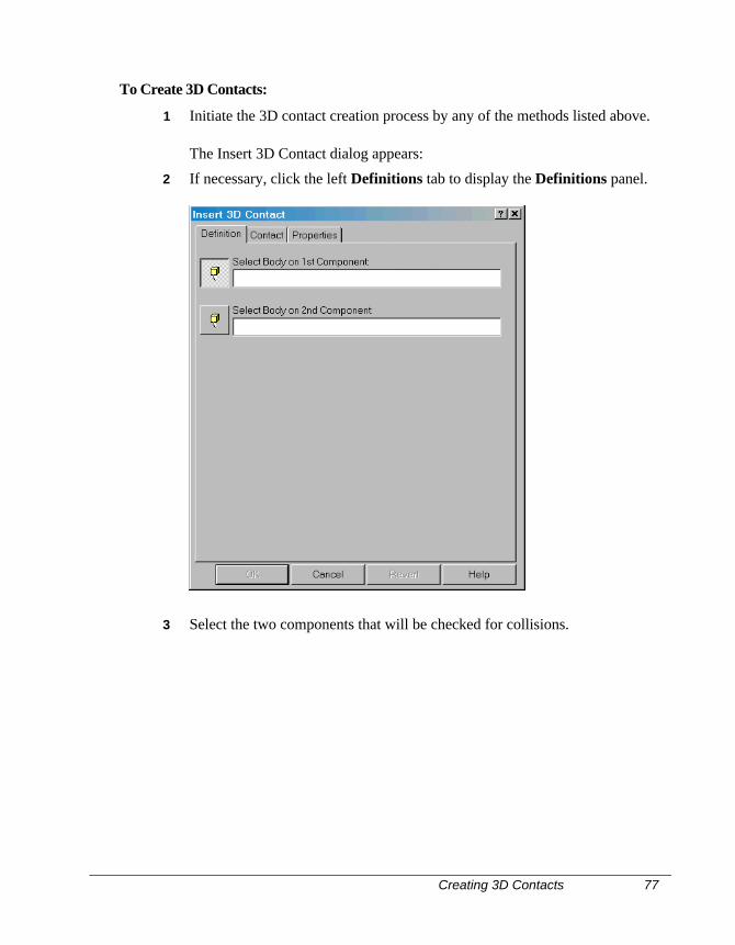
Creating 3D Contacts 77
To Create 3D Contacts:
1 Initiate the 3D contact creation process by any of the methods listed above.
The Insert 3D Contact dialog appears:
2 If necessary, click the left Definitions tab to display the Definitions panel.
3 Select the two components that will be checked for collisions.
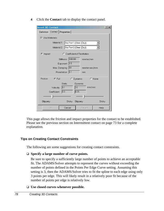
78 Creating 3D Contacts
4 Click the Contact tab to display the contact panel.
This page allows the friction and impact properties for the contact to be established.Please see the previous section on Intermittent contact on page 73 for a completeexplanation.
Tips on Creating Contact Constraints
The following are some suggestions for creating contact constraints.
q Specify a large number of curve points.Be sure to specify a sufficiently large number of points to achieve an acceptablefit. The ADAMS/Solver attempts to represent the curves without exceeding thenumber of points defined in the Points Per Edge Curve setting. Assuming thissetting is 3, then the ADAMS/Solver tries to fit the spline to each edge using only3 points per edge. This will likely result in a relatively poor fit because of thenumber of points per edge is relatively low.
q Use closed curves whenever possible.
Joint Couplers 79
It is generally easier to select a closed curve if possible. Open curves representmodeling difficulties when the point on the follower rigid body approaches one ofthe end points of the open curve. Closed curves have no beginning and endingpoints, and, therefore, avoid this numerically difficult situation.
q Avoid defining the initial configuration of a point-curve constraint with thepoint near to one of the end points of the curve.
q Avoid highly nonlinear edges.
Joint Couplers
Joint couplers allow the motion of a revolute, cylindrical, or translational joint to be"coupled" to the motion of another revolute, cylindrical or translational joints. Thetwo coupled joints may be of the same type, or the may be different types, forexample a revolute joint may be coupled to a translational joint. The coupled motionmay also be of the same type, or may be a different type. For example, the rotarymotion of a revolute joint may be coupled to the rotary motion of a cylindrical joint,or the translational motion of a translational joint may be coupled to the rotarymotion of a cylindrical joint.
A coupler takes to value, one for the motion of each joint, and from these derives aratio that relates the motion of one joint to the motion of another joint. For example,if a revolute joint is being coupled with a translational joint, 90 degrees could bespecified for the revolute joint, and 100 mm for the translational joint. This meansthat for every 90 degrees the revolute joint rotates, the translational joint will bemoved 100 mm, or 1 degree of rotation results in 0.9 mm of translation (90/100).
A coupler does not differentiate between a "driver" joint and a "driven" joint. Eitherjoint in the couple may at one point in time be "driving" the other joint. A potentialfor locking does exist if both joints in a couple are driven by motion generators. Thecouple may conflict with the motion generator.
A single joint may be coupled to more than one joint. Again, the potential for lockingdoes exist if the multiple couples conflict with each other.
A coupler removes one additional degree of freedom from the Motion Model.
A joint coupler may be created by one of the following methods:
• Choosing Motion, Couplers from the Menu.
• Selecting the Couplers branch in the Browser and choosing Add Coupler from
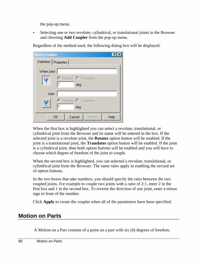
80 Motion on Parts
the pop-up menu.
• Selecting one or two revolute, cylindrical, or translational joints in the Browserand choosing Add Coupler from the pop-up menu.
Regardless of the method used, the following dialog box will be displayed:
When the first box is highlighted you can select a revolute, translational, orcylindrical joint from the Browser and its name will be entered in the box. If theselected joint is a revolute joint, the Rotates option button will be enabled. If thejoint is a translational joint, the Translates option button will be enabled. If the jointis a cylindrical joint, then both option buttons will be enabled and you will have tochoose which degree of freedom of the joint to couple.
When the second box is highlighted, you can selected a revolute, translational, orcylindrical joint from the Browser. The same rules apply in enabling the second setof option buttons.
In the two boxes that take numbers, you should specify the ratio between the twocoupled joints. For example to couple two joints with a ratio of 2:1, enter 2 in thefirst box and 1 in the second box. To reverse the direction of one joint, enter a minussign in front of the number.
Click Apply to create the coupler when all of the parameters have been specified.
Motion on Parts
A Motion on a Part consists of a point on a part with six (6) degrees of freedom.
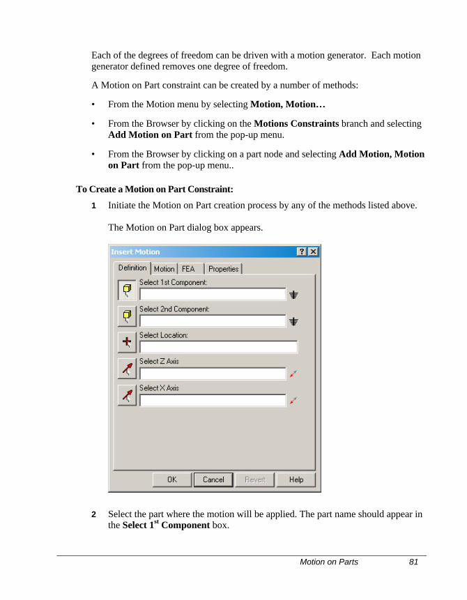
Motion on Parts 81
Each of the degrees of freedom can be driven with a motion generator. Each motiongenerator defined removes one degree of freedom.
A Motion on Part constraint can be created by a number of methods:
• From the Motion menu by selecting Motion, Motion…
• From the Browser by clicking on the Motions Constraints branch and selectingAdd Motion on Part from the pop-up menu.
• From the Browser by clicking on a part node and selecting Add Motion, Motionon Part from the pop-up menu..
To Create a Motion on Part Constraint:
1 Initiate the Motion on Part creation process by any of the methods listed above.
The Motion on Part dialog box appears.
2 Select the part where the motion will be applied. The part name should appear inthe Select 1st Component box.
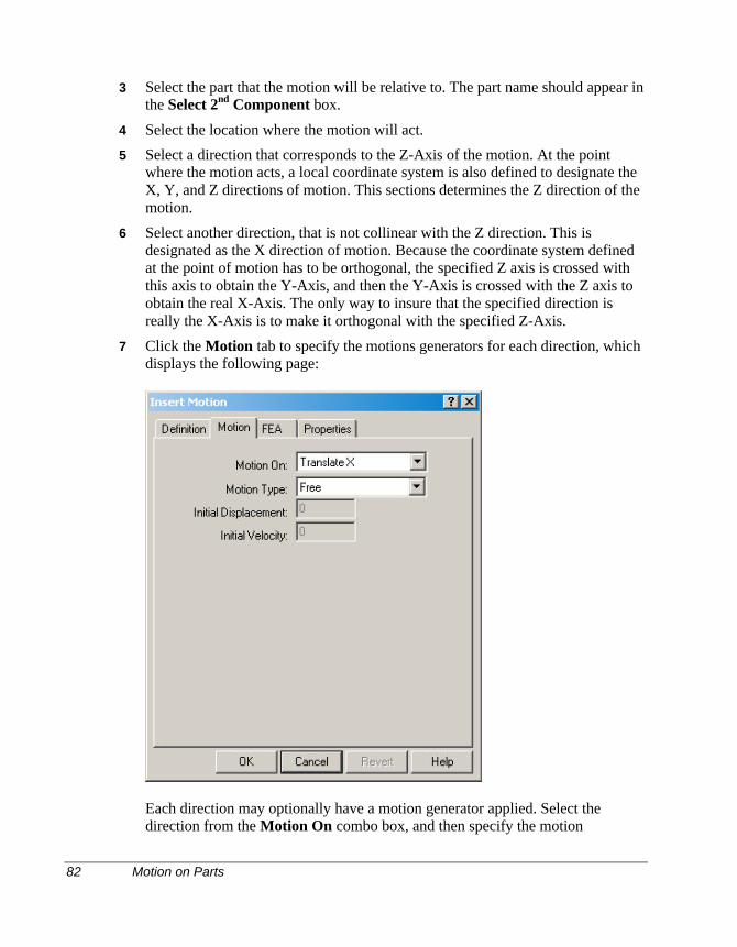
82 Motion on Parts
3 Select the part that the motion will be relative to. The part name should appear inthe Select 2nd Component box.
4 Select the location where the motion will act.
5 Select a direction that corresponds to the Z-Axis of the motion. At the pointwhere the motion acts, a local coordinate system is also defined to designate theX, Y, and Z directions of motion. This sections determines the Z direction of themotion.
6 Select another direction, that is not collinear with the Z direction. This isdesignated as the X direction of motion. Because the coordinate system definedat the point of motion has to be orthogonal, the specified Z axis is crossed withthis axis to obtain the Y-Axis, and then the Y-Axis is crossed with the Z axis toobtain the real X-Axis. The only way to insure that the specified direction isreally the X-Axis is to make it orthogonal with the specified Z-Axis.
7 Click the Motion tab to specify the motions generators for each direction, whichdisplays the following page:
Each direction may optionally have a motion generator applied. Select thedirection from the Motion On combo box, and then specify the motion
Rigid Bodies 83
parameters. These parameters are the same as described on Page 52.
Rigid Bodies
In Dynamic Designer/Motion, a rigid body can be a single Solid Edge part or a sub-assembly. The term rigid body means that the individual components that make upthe rigid body are rigidly attached to each other: during animation, they movetogether as they move with respect to other rigid bodies.
Ground
The ground rigid body is unique. It is by definition at absolute rest. All mechanismshave a ground rigid body. It serves as the reference frame for the remaining rigidbodies. All non-grounded rigid bodies in your mechanism move with respect toground.
Mass properties
The mass properties by default are directly defined by the solids in your Solid Edgeassembly.
Mass properties are important in Dynamic Designer/Motion because inertial loadseffect reaction loads in joints that could be used as inputs for structural analysis.
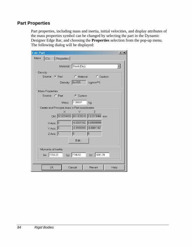
84 Rigid Bodies
Part Properties
Part properties, including mass and inertia, initial velocities, and display attributes ofthe mass properties symbol can be changed by selecting the part in the DynamicDesigner Edge Bar, and choosing the Properties selection from the pop-up menu.The following dialog will be displayed:
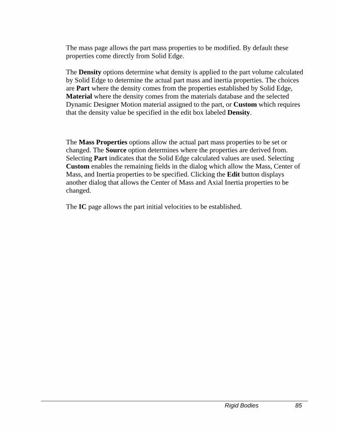
Rigid Bodies 85
The mass page allows the part mass properties to be modified. By default theseproperties come directly from Solid Edge.
The Density options determine what density is applied to the part volume calculatedby Solid Edge to determine the actual part mass and inertia properties. The choicesare Part where the density comes from the properties established by Solid Edge,Material where the density comes from the materials database and the selectedDynamic Designer Motion material assigned to the part, or Custom which requiresthat the density value be specified in the edit box labeled Density.
The Mass Properties options allow the actual part mass properties to be set orchanged. The Source option determines where the properties are derived from.Selecting Part indicates that the Solid Edge calculated values are used. SelectingCustom enables the remaining fields in the dialog which allow the Mass, Center ofMass, and Inertia properties to be specified. Clicking the Edit button displaysanother dialog that allows the Center of Mass and Axial Inertia properties to bechanged.
The IC page allows the part initial velocities to be established.
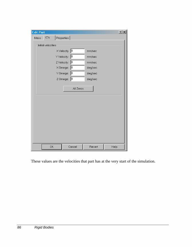
86 Rigid Bodies
These values are the velocities that part has at the very start of the simulation.
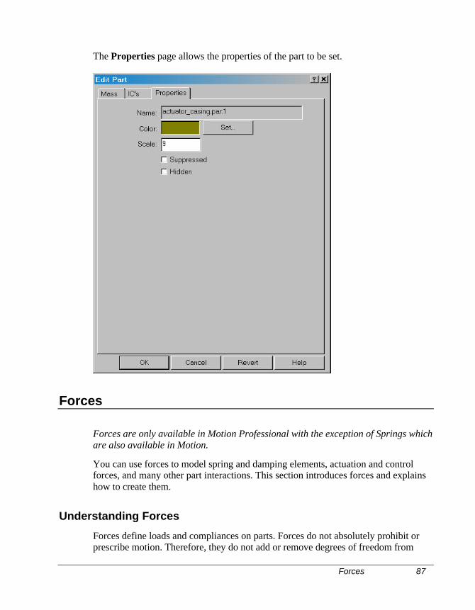
Forces 87
The Properties page allows the properties of the part to be set.
Forces
Forces are only available in Motion Professional with the exception of Springs whichare also available in Motion.
You can use forces to model spring and damping elements, actuation and controlforces, and many other part interactions. This section introduces forces and explainshow to create them.
Understanding Forces
Forces define loads and compliances on parts. Forces do not absolutely prohibit orprescribe motion. Therefore, they do not add or remove degrees of freedom from
88 Forces
your model. Forces may resist motion, such as springs or dampers, or they mayinduce motion.
Dynamic Designer provides the following type of forces:
q Applied Forces - Applied forces are forces that define loads and compliances onparts so that they move in certain ways. Applied forces are very general, but youmust supply your own description of the force behavior by specifying a constantforce value or function expression. The applied forces in DynamicDesigner/Motion are the applied force, applied torque, action/reaction force, andaction/reaction torque.
q Flexible Connectors - Flexible connectors resist motion and are simpler andeasier to use than applied forces because you only supply constant coefficients forthe forces. The flexible connectors include translational springs, torsion springs,translational dampers, and torsion dampers.
q Gravity - For more information on gravity and setting gravity, see the Gravitysection below.
For every force that you create in Dynamic Designer/Motion, you specify thefollowing information:
q Whether the force is translational or rotational.
q Which part or parts is the force applied.
q At what point or points is the force applied.
q Magnitude and direction of the force.
The following sections explain in more detail how to define the magnitude anddirection of forces.
Force Magnitude
A force function specifies the force magnitude throughout your simulation. You candefine force magnitudes in Dynamic Designer/Motion in the following ways:
q Enter values used to define stiffness and damping coefficients (springs anddampers only). In this case, Dynamic Designer automatically makes the forcemagnitude proportional to the distance or velocity between two points. Thecoefficients represent the proportionality constants.
q Enter a function expression using one of the pre-defined functions.
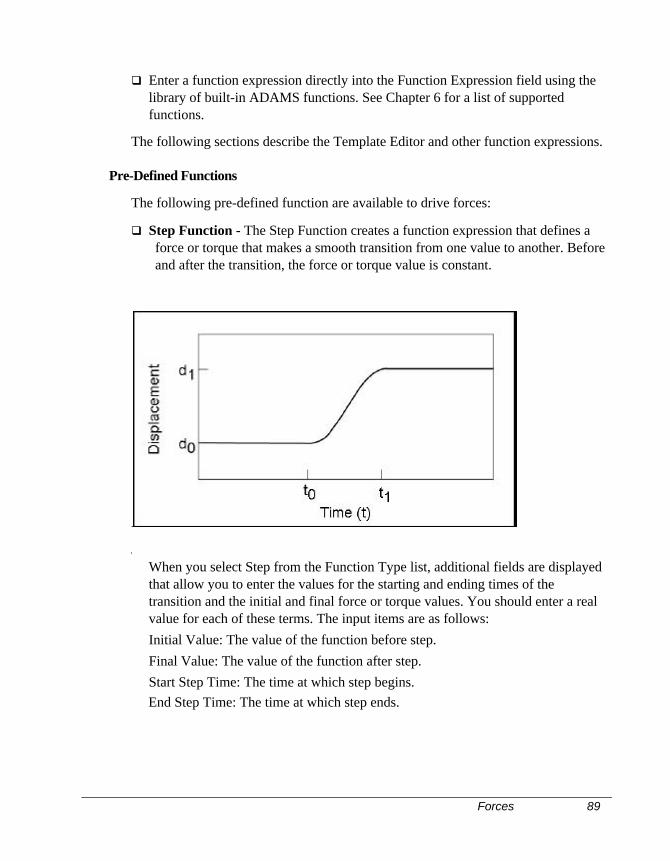
Forces 89
q Enter a function expression directly into the Function Expression field using thelibrary of built-in ADAMS functions. See Chapter 6 for a list of supportedfunctions.
The following sections describe the Template Editor and other function expressions.
Pre-Defined Functions
The following pre-defined function are available to drive forces:
q Step Function - The Step Function creates a function expression that defines aforce or torque that makes a smooth transition from one value to another. Beforeand after the transition, the force or torque value is constant.
When you select Step from the Function Type list, additional fields are displayedthat allow you to enter the values for the starting and ending times of thetransition and the initial and final force or torque values. You should enter a realvalue for each of these terms. The input items are as follows:Initial Value: The value of the function before step.Final Value: The value of the function after step.Start Step Time: The time at which step begins.End Step Time: The time at which step ends.
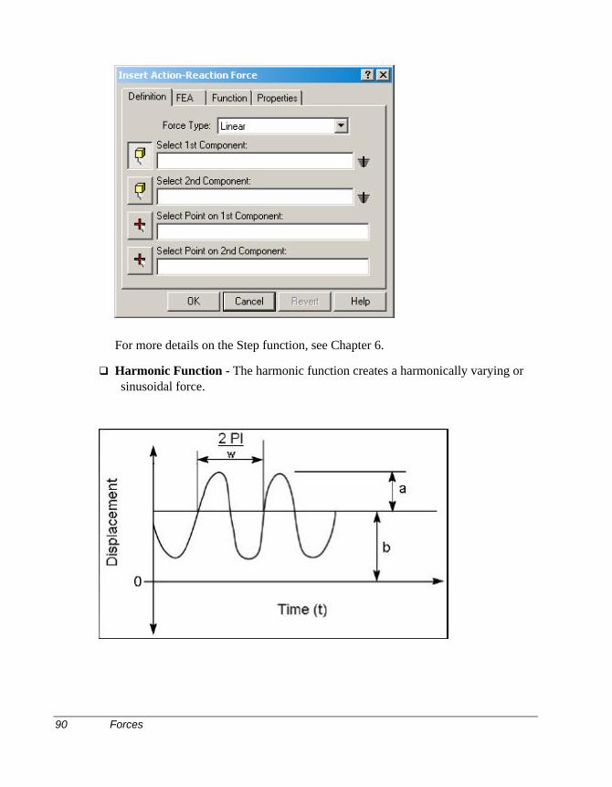
90 Forces
For more details on the Step function, see Chapter 6.
q Harmonic Function - The harmonic function creates a harmonically varying orsinusoidal force.
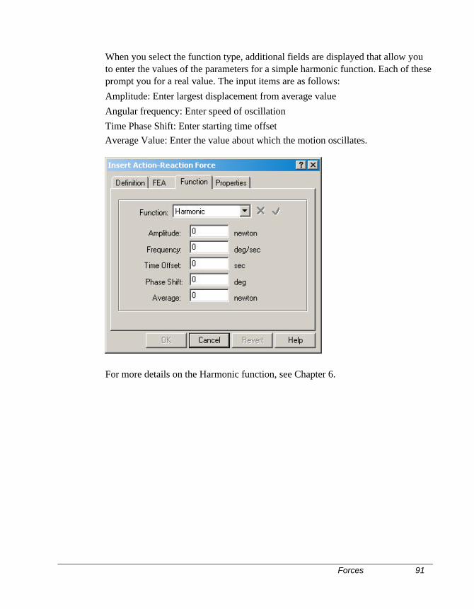
Forces 91
When you select the function type, additional fields are displayed that allow youto enter the values of the parameters for a simple harmonic function. Each of theseprompt you for a real value. The input items are as follows:Amplitude: Enter largest displacement from average valueAngular frequency: Enter speed of oscillationTime Phase Shift: Enter starting time offsetAverage Value: Enter the value about which the motion oscillates.
For more details on the Harmonic function, see Chapter 6.
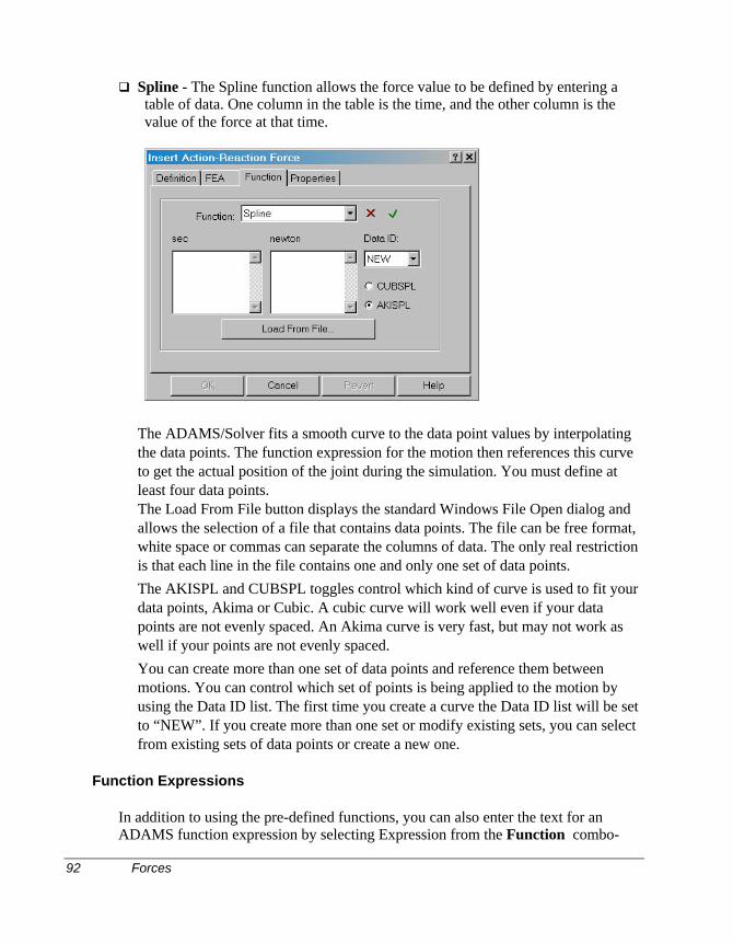
92 Forces
q Spline - The Spline function allows the force value to be defined by entering atable of data. One column in the table is the time, and the other column is thevalue of the force at that time.
The ADAMS/Solver fits a smooth curve to the data point values by interpolatingthe data points. The function expression for the motion then references this curveto get the actual position of the joint during the simulation. You must define atleast four data points.The Load From File button displays the standard Windows File Open dialog andallows the selection of a file that contains data points. The file can be free format,white space or commas can separate the columns of data. The only real restrictionis that each line in the file contains one and only one set of data points.The AKISPL and CUBSPL toggles control which kind of curve is used to fit yourdata points, Akima or Cubic. A cubic curve will work well even if your datapoints are not evenly spaced. An Akima curve is very fast, but may not work aswell if your points are not evenly spaced.You can create more than one set of data points and reference them betweenmotions. You can control which set of points is being applied to the motion byusing the Data ID list. The first time you create a curve the Data ID list will be setto “NEW”. If you create more than one set or modify existing sets, you can selectfrom existing sets of data points or create a new one.
Function Expressions
In addition to using the pre-defined functions, you can also enter the text for anADAMS function expression by selecting Expression from the Function combo-
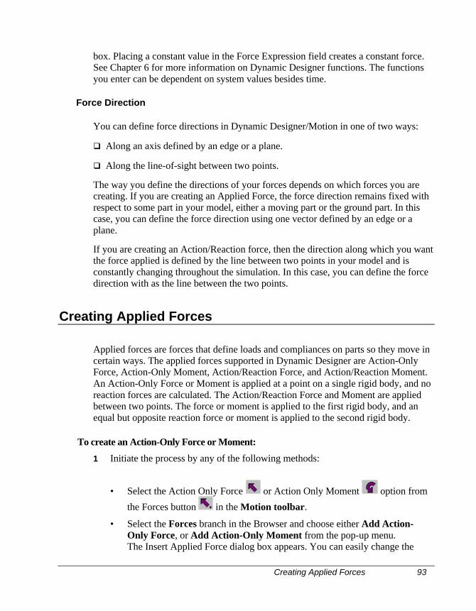
Creating Applied Forces 93
box. Placing a constant value in the Force Expression field creates a constant force.See Chapter 6 for more information on Dynamic Designer functions. The functionsyou enter can be dependent on system values besides time.
Force Direction
You can define force directions in Dynamic Designer/Motion in one of two ways:
q Along an axis defined by an edge or a plane.
q Along the line-of-sight between two points.
The way you define the directions of your forces depends on which forces you arecreating. If you are creating an Applied Force, the force direction remains fixed withrespect to some part in your model, either a moving part or the ground part. In thiscase, you can define the force direction using one vector defined by an edge or aplane.
If you are creating an Action/Reaction force, then the direction along which you wantthe force applied is defined by the line between two points in your model and isconstantly changing throughout the simulation. In this case, you can define the forcedirection with as the line between the two points.
Creating Applied Forces
Applied forces are forces that define loads and compliances on parts so they move incertain ways. The applied forces supported in Dynamic Designer are Action-OnlyForce, Action-Only Moment, Action/Reaction Force, and Action/Reaction Moment.An Action-Only Force or Moment is applied at a point on a single rigid body, and noreaction forces are calculated. The Action/Reaction Force and Moment are appliedbetween two points. The force or moment is applied to the first rigid body, and anequal but opposite reaction force or moment is applied to the second rigid body.
To create an Action-Only Force or Moment:
1 Initiate the process by any of the following methods:
• Select the Action Only Force or Action Only Moment option from
the Forces button in the Motion toolbar.
• Select the Forces branch in the Browser and choose either Add Action-Only Force, or Add Action-Only Moment from the pop-up menu.The Insert Applied Force dialog box appears. You can easily change the
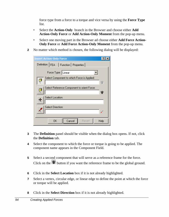
94 Creating Applied Forces
force type from a force to a torque and vice versa by using the Force Typelist.
• Select the Action-Only branch in the Browser and choose either AddAction-Only Force or Add Action-Only Moment from the pop-up menu.
• Select one moving part in the Browser ad choose either Add Force Action-Only Force or Add Force Action-Only Moment from the pop-up menu.
2 No matter which method is chosen, the following dialog will be displayed:
3 The Definition panel should be visible when the dialog box opens. If not, clickthe Definition tab.
4 Select the component to which the force or torque is going to be applied. Thecomponent name appears in the Component Field.
5 Select a second component that will serve as a reference frame for the force.
Click on the button if you want the reference frame to be the global ground.
6 Click in the Select Location box if it is not already highlighted.
7 Select a vertex, circular edge, or linear edge to define the point at which the forceor torque will be applied.
8 Click in the Select Direction box if it is not already highlighted.
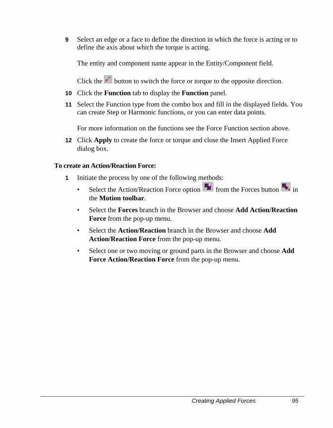
Creating Applied Forces 95
9 Select an edge or a face to define the direction in which the force is acting or todefine the axis about which the torque is acting.
The entity and component name appear in the Entity/Component field.
Click the button to switch the force or torque to the opposite direction.
10 Click the Function tab to display the Function panel.
11 Select the Function type from the combo box and fill in the displayed fields. Youcan create Step or Harmonic functions, or you can enter data points.
For more information on the functions see the Force Function section above.
12 Click Apply to create the force or torque and close the Insert Applied Forcedialog box.
To create an Action/Reaction Force:
1 Initiate the process by one of the following methods:
• Select the Action/Reaction Force option from the Forces button inthe Motion toolbar.
• Select the Forces branch in the Browser and choose Add Action/ReactionForce from the pop-up menu.
• Select the Action/Reaction branch in the Browser and choose AddAction/Reaction Force from the pop-up menu.
• Select one or two moving or ground parts in the Browser and choose AddForce Action/Reaction Force from the pop-up menu.
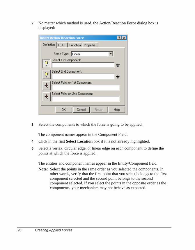
96 Creating Applied Forces
2 No matter which method is used, the Action/Reaction Force dialog box isdisplayed:
3 Select the components to which the force is going to be applied.
The component names appear in the Component Field.
4 Click in the first Select Location box if it is not already highlighted.
5 Select a vertex, circular edge, or linear edge on each component to define thepoints at which the force is applied.
The entities and component names appear in the Entity/Component field.Note: Select the points in the same order as you selected the components. In
other words, verify that the first point that you select belongs to the firstcomponent selected and the second point belongs to the secondcomponent selected. If you select the points in the opposite order as thecomponents, your mechanism may not behave as expected.
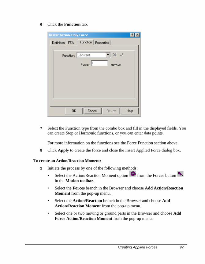
Creating Applied Forces 97
6 Click the Function tab.
7 Select the Function type from the combo box and fill in the displayed fields. Youcan create Step or Harmonic functions, or you can enter data points.
For more information on the functions see the Force Function section above.
8 Click Apply to create the force and close the Insert Applied Force dialog box.
To create an Action/Reaction Moment:
1 Initiate the process by one of the following methods:
• Select the Action/Reaction Moment option from the Forces button in the Motion toolbar.
• Select the Forces branch in the Browser and choose Add Action/ReactionMoment from the pop-up menu.
• Select the Action/Reaction branch in the Browser and choose AddAction/Reaction Moment from the pop-up menu.
• Select one or two moving or ground parts in the Browser and choose AddForce Action/Reaction Moment from the pop-up menu.
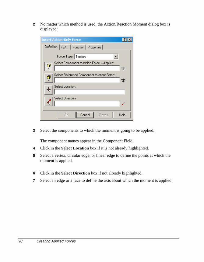
98 Creating Applied Forces
2 No matter which method is used, the Action/Reaction Moment dialog box isdisplayed:
3 Select the components to which the moment is going to be applied.
The component names appear in the Component Field.
4 Click in the Select Location box if it is not already highlighted.
5 Select a vertex, circular edge, or linear edge to define the points at which themoment is applied.
6 Click in the Select Direction box if not already highlighted.
7 Select an edge or a face to define the axis about which the moment is applied.
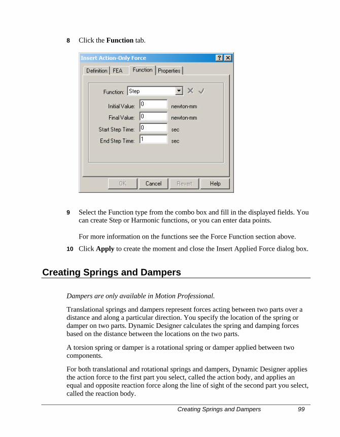
Creating Springs and Dampers 99
8 Click the Function tab.
9 Select the Function type from the combo box and fill in the displayed fields. Youcan create Step or Harmonic functions, or you can enter data points.
For more information on the functions see the Force Function section above.
10 Click Apply to create the moment and close the Insert Applied Force dialog box.
Creating Springs and Dampers
Dampers are only available in Motion Professional.
Translational springs and dampers represent forces acting between two parts over adistance and along a particular direction. You specify the location of the spring ordamper on two parts. Dynamic Designer calculates the spring and damping forcesbased on the distance between the locations on the two parts.
A torsion spring or damper is a rotational spring or damper applied between twocomponents.
For both translational and rotational springs and dampers, Dynamic Designer appliesthe action force to the first part you select, called the action body, and applies anequal and opposite reaction force along the line of sight of the second part you select,called the reaction body.
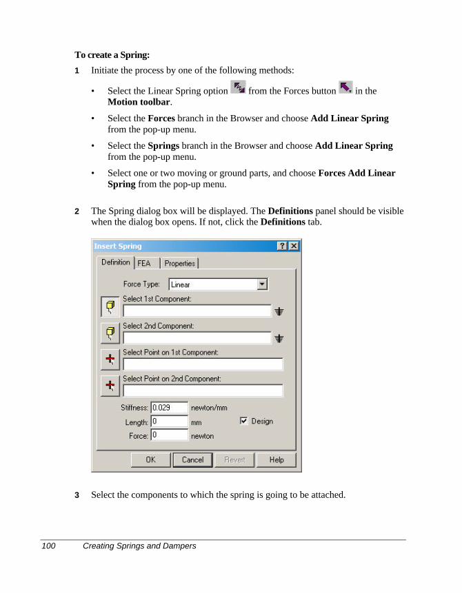
100 Creating Springs and Dampers
To create a Spring:
1 Initiate the process by one of the following methods:
• Select the Linear Spring option from the Forces button in theMotion toolbar.
• Select the Forces branch in the Browser and choose Add Linear Springfrom the pop-up menu.
• Select the Springs branch in the Browser and choose Add Linear Springfrom the pop-up menu.
• Select one or two moving or ground parts, and choose Forces Add LinearSpring from the pop-up menu.
2 The Spring dialog box will be displayed. The Definitions panel should be visiblewhen the dialog box opens. If not, click the Definitions tab.
3 Select the components to which the spring is going to be attached.
Creating Springs and Dampers 101
4 Click in the first Select Location box if not already highlighted.
5 Select a vertex, circular edge, or linear edge on the first component you selectedto define the point at which the spring is attached.
The entity and component name appears in the Entity/Component field.
6 Click in the second Select Location box if not already highlighted and thenselect a vertex, circular edge, or linear edge on the second component youselected to define the other point at which the spring is attached.Note: Verify that your first point is on the first component and the second point
is on the second component. If you select the points out of order with thecomponents, your spring will not behave as expected.
7 Modify the default spring stiffness by clicking in the Stiffness field and enteringa new value.
8 By toggling the Design toggle off, you can define the free length of the spring. Ifyou leave the Design toggle on, the free length of the spring is automaticallydefined to be the distance between the two points that you selected in the Pointspanel.Note: The free length of the spring is the distance between those points in the
initial position of the assembly.
9 You can define a preload on the spring by entering a value in the Force field.
10 Click Apply to create the spring and close the Insert Spring dialog box.
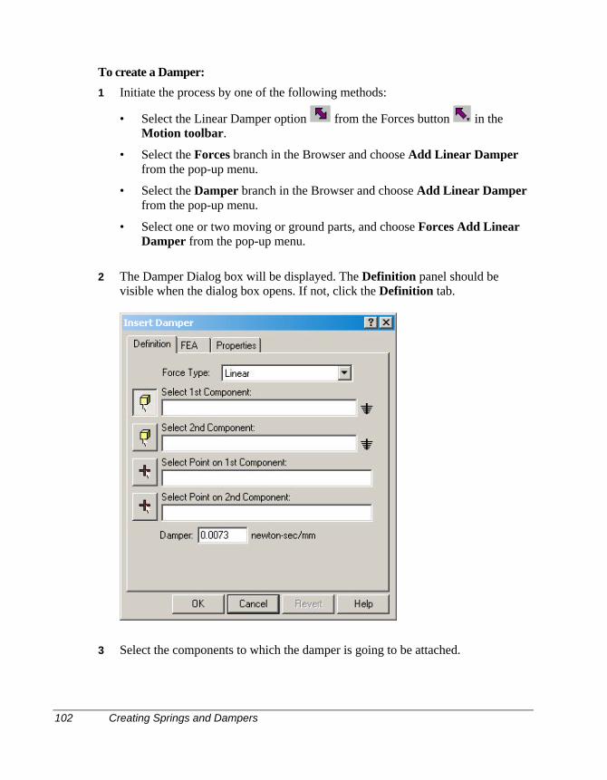
102 Creating Springs and Dampers
To create a Damper:
1 Initiate the process by one of the following methods:
• Select the Linear Damper option from the Forces button in theMotion toolbar.
• Select the Forces branch in the Browser and choose Add Linear Damperfrom the pop-up menu.
• Select the Damper branch in the Browser and choose Add Linear Damperfrom the pop-up menu.
• Select one or two moving or ground parts, and choose Forces Add LinearDamper from the pop-up menu.
2 The Damper Dialog box will be displayed. The Definition panel should bevisible when the dialog box opens. If not, click the Definition tab.
3 Select the components to which the damper is going to be attached.

Creating Springs and Dampers 103
4 Click in the first Select Location box if not already highlighted.
5 Select a vertex, circular edge, or linear edge on the first component you selectedto define the point at which the damper is attached.
6 Click in the second Select Location box if not already highlighted and thenselect a vertex, circular edge, or linear edge on the second component youselected to define the other point at which the damper is attached.Note: Verify that your first point is on the first component and the second point
is on the second component. If you select the points out of order with thecomponents, your damper will not behave as expected.
7 Modify the default damping coefficient by clicking in the Damping field andentering a new value.
8 Click Apply to create the damper and close the Insert Damper dialog box.
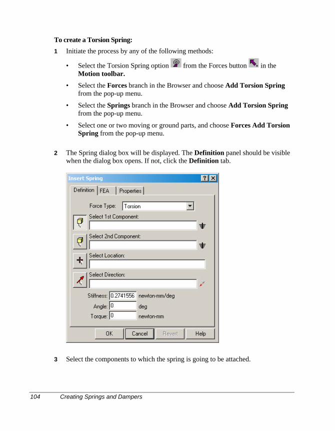
104 Creating Springs and Dampers
To create a Torsion Spring:
1 Initiate the process by any of the following methods:
• Select the Torsion Spring option from the Forces button in theMotion toolbar.
• Select the Forces branch in the Browser and choose Add Torsion Springfrom the pop-up menu.
• Select the Springs branch in the Browser and choose Add Torsion Springfrom the pop-up menu.
• Select one or two moving or ground parts, and choose Forces Add TorsionSpring from the pop-up menu.
2 The Spring dialog box will be displayed. The Definition panel should be visiblewhen the dialog box opens. If not, click the Definition tab.
3 Select the components to which the spring is going to be attached.
Creating Springs and Dampers 105
4 Click in the Select Location box if not already highlighted.
5 Select a vertex, circular edge, or linear edge to define the point at which thespring is attached.
The entity and component name appears in the Entity/Component field.
6 Click in the Select Direction box if not already highlighted.
7 Select an edge or a face to define the axis about which the spring is acting.
The entity and component name appear in the Entity/Component field. Click the button to switch the spring to the opposite direction.
8 Modify the default spring stiffness by clicking in the Stiffness field and enteringa new value.
9 You can define the preload angle of the spring by entering a value in the Anglefield. By default, the angle is set to zero, the angle in the design position.
10 You can define a preload on the spring by entering a value in the Torque field.
11 Click Apply to create the spring and close the Insert Spring Torque dialog box.

106 Creating Springs and Dampers
To create a Torsion Damper:
1 Initiate the process by one of the following methods:
• Select the Torsion Damper option from the Forces button in theMotion toolbar.
• Select the Forces branch in the Browser and choose Add Torsion Damperfrom the pop-up menu.
• Select the Springs branch in the Browser and choose Add Torsion Damperfrom the pop-up menu.
• Select one or two moving or ground parts, and choose Forces Add TorsionDamper from the pop-up menu.
2 The Damper Dialog box will be displayed. The Definition panel should bevisible when the dialog box opens. If not, click the Definition tab.
3 Select the components to which the damper is going to be attached.
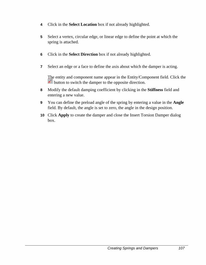
Creating Springs and Dampers 107
4 Click in the Select Location box if not already highlighted.
5 Select a vertex, circular edge, or linear edge to define the point at which thespring is attached.
6 Click in the Select Direction box if not already highlighted.
7 Select an edge or a face to define the axis about which the damper is acting.
The entity and component name appear in the Entity/Component field. Click the button to switch the damper to the opposite direction.
8 Modify the default damping coefficient by clicking in the Stiffness field andentering a new value.
9 You can define the preload angle of the spring by entering a value in the Anglefield. By default, the angle is set to zero, the angle in the design position.
10 Click Apply to create the damper and close the Insert Torsion Damper dialogbox.
108 Creating Impact Forces
Creating Impact ForcesImpact forces are only available in Motion Professional.
Impact forces are used to simulate the collision between two parts. As two partsapproach within a specified distance, the impact force becomes active, and a forcespecified by the impact parameters will be applied to both of the colliding parts.
An impact force is controlled by the following five parameters:
Distance The distance from the contact point on the first link, to the force actionpoint on the first part (the point that was graphically identified). Thiscan be thought of as a sphere of radius <distance> centered at the actionpoint of the force. During the simulation, when the distance between theimpact point on the second part is equal to this parameter, then impactwill occur.
Stiffness This is the stiffness of the boundary interaction between the two parts. Itshould be set to a number that approximates the material stiffness of thetwo parts in collision.
Exponent The exponent of the force deformation characteristic. Dynamic DesignerMotion models the collision using an exponential force function.
Max Damping The maximum damping coefficient of the boundary interaction.
Penetration The boundary penetration distance where full damping will occur.
When the distance between the points is reached, and the impact force becomesactive, it produces a force that is a function of the relative velocity of the two parts towhich the force is attached. The graph below shows an example:
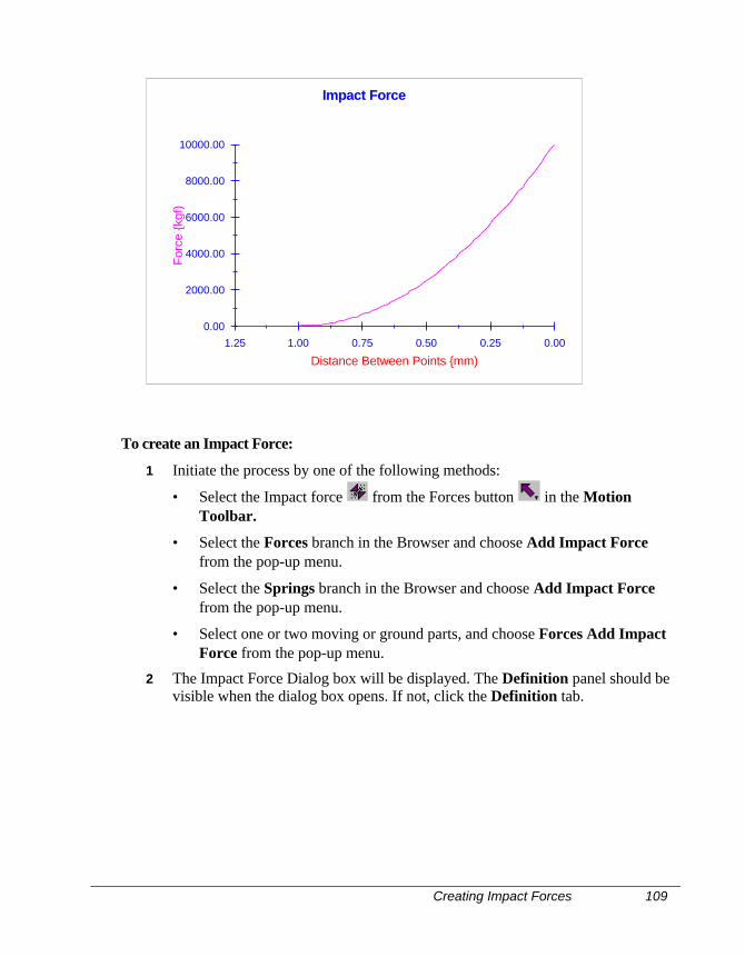
Creating Impact Forces 109
1.25 1.00 0.75 0.50 0.25 0.00
Distance Between Points {mm)
0.00
2000.00
4000.00
6000.00
8000.00
10000.00
For
ce {k
gf)
Impact Force
To create an Impact Force:
1 Initiate the process by one of the following methods:
• Select the Impact force from the Forces button in the MotionToolbar.
• Select the Forces branch in the Browser and choose Add Impact Forcefrom the pop-up menu.
• Select the Springs branch in the Browser and choose Add Impact Forcefrom the pop-up menu.
• Select one or two moving or ground parts, and choose Forces Add ImpactForce from the pop-up menu.
2 The Impact Force Dialog box will be displayed. The Definition panel should bevisible when the dialog box opens. If not, click the Definition tab.
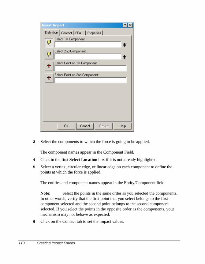
110 Creating Impact Forces
3 Select the components to which the force is going to be applied.
The component names appear in the Component Field.
4 Click in the first Select Location box if it is not already highlighted.
5 Select a vertex, circular edge, or linear edge on each component to define thepoints at which the force is applied.
The entities and component names appear in the Entity/Component field.
Note: Select the points in the same order as you selected the components.In other words, verify that the first point that you select belongs to the firstcomponent selected and the second point belongs to the second componentselected. If you select the points in the opposite order as the components, yourmechanism may not behave as expected.
6 Click on the Contact tab to set the impact values.
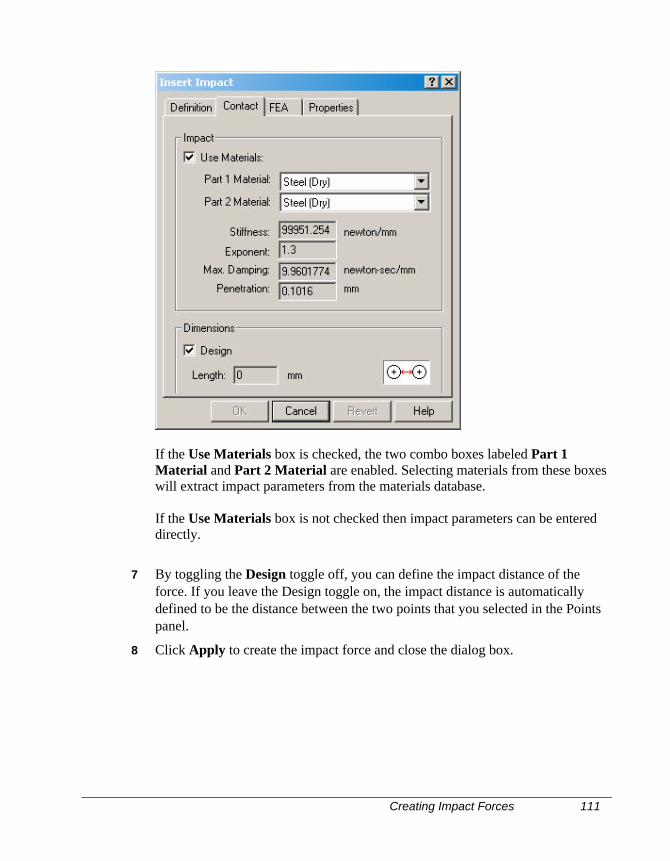
Creating Impact Forces 111
If the Use Materials box is checked, the two combo boxes labeled Part 1Material and Part 2 Material are enabled. Selecting materials from these boxeswill extract impact parameters from the materials database.
If the Use Materials box is not checked then impact parameters can be entereddirectly.
7 By toggling the Design toggle off, you can define the impact distance of theforce. If you leave the Design toggle on, the impact distance is automaticallydefined to be the distance between the two points that you selected in the Pointspanel.
8 Click Apply to create the impact force and close the dialog box.

112 Gravity
Gravity
Gravity is applied to your entire model uniformly. Gravity is defined by a value and adirection. By default, gravity is 9.81 meters per second squared (or the equivalent inother units) in the negative Y direction in the design coordinate system.
To Modify the Gravity Setting:
1 Use the Options button from Motion Toolbar, or click the Motion Modelbranch in the Browser and choose System Defaults from the pop-up menu.Either method will open the Dynamic Designer Options dialog box. You canalso open the Setting dialog box by clicking on the Options button on theSimulation tool bar, next to the Simulate button and directly above the DOFcounter.
2 If the World panel isn’t visible, click the World tab to display it.
3 You can modify the gravity settings by selecting one of the options in theAcceleration list. You can turn the gravity force off by selecting Off, you can setit to be the standard gravity value for earth by selecting Earth Standard, or youcan set the acceleration to Custom.
4 If you set the Acceleration setting to Custom, you can enter your own gravityvalues in the X, Y, and Z fields below the Acceleration setting.
5 Click OK to modify gravity and close the Dynamic Designer Options dialogbox.
Manipulating Mechanism Entities 113
Manipulating Mechanism Entities
You can easily modify or delete mechanism entities in Dynamic Designer/Motion.
Editing Mechanism Elements
You can edit any Dynamic Designer Motion object. The parameters you can edit areusually the same as those you define when the object is created.
To Edit a Dynamic Designer/Motion element:
1 Select the element in the IntelliMotion Browser.
2 Choose Properties from the pop-up menu.
The Edit panel appears.
3 Edit the attribute that you want to edit and click Apply to complete the edit andclose the dialog box.
4 To replace a component, location or direction field for a motion entity, select thefield (so that it is highlighted) and then press the “Delete” key on the keyboard.This will clear the field. Now pick the object to replace the once just cleared.
Deleting Mechanism Elements
The IntelliMotion Browser is used to delete Motion object from your mechanism.
To delete a mechanism element:
1 Select the element in the IntelliMotion Browser.
2 Choose Delete from the pop-up menu. Alternatively, you can also press the“Delete” key on the keyboard to delete the highlighted entities in the browser.

Adding Materials 115
Dynamic Designer Motion supports a materials database capability. The database isprimarily intended to define interaction properties between material types, but it alsocontains some basic material property information. The interaction properties areused by impact forces, intermittent contact, and joint friction.
Adding Materials
The database supplied with Dynamic Designer Motion contains property informationfor some common materials. It is also possible to add new material information to thedatabase.
A new material can be added to the database by clicking on the Motion Model rootnode in the Browser and choosing Materials->Add from the pop-up menu.
The Add Materials wizard will be started. The first page in the wizard is:
3 Materials
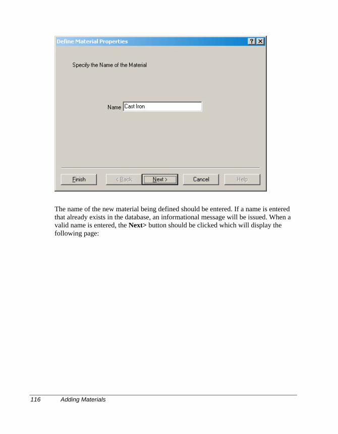
116 Adding Materials
The name of the new material being defined should be entered. If a name is enteredthat already exists in the database, an informational message will be issued. When avalid name is entered, the Next> button should be clicked which will display thefollowing page:
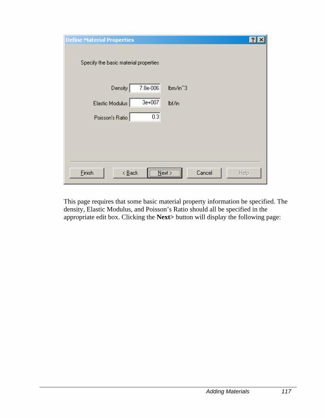
Adding Materials 117
This page requires that some basic material property information be specified. Thedensity, Elastic Modulus, and Poisson’s Ratio should all be specified in theappropriate edit box. Clicking the Next> button will display the following page:
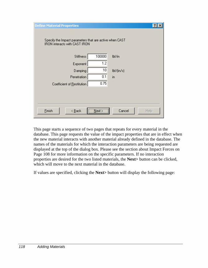
118 Adding Materials
This page starts a sequence of two pages that repeats for every material in thedatabase. This page requests the value of the impact properties that are in effect whenthe new material interacts with another material already defined in the database. Thenames of the materials for which the interaction parameters are being requested aredisplayed at the top of the dialog box. Please see the section about Impact Forces onPage 108 for more information on the specific parameters. If no interactionproperties are desired for the two listed materials, the Next> button can be clicked,which will move to the next material in the database.
If values are specified, clicking the Next> button will display the following page:
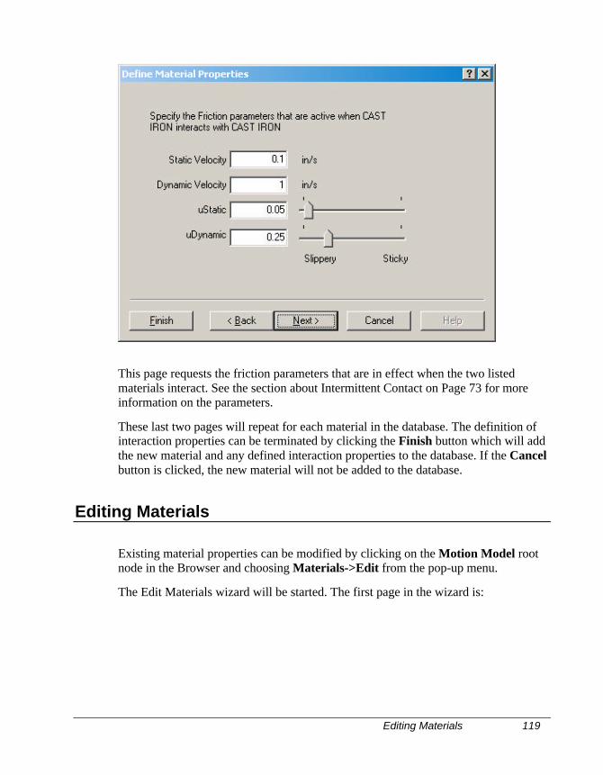
Editing Materials 119
This page requests the friction parameters that are in effect when the two listedmaterials interact. See the section about Intermittent Contact on Page 73 for moreinformation on the parameters.
These last two pages will repeat for each material in the database. The definition ofinteraction properties can be terminated by clicking the Finish button which will addthe new material and any defined interaction properties to the database. If the Cancelbutton is clicked, the new material will not be added to the database.
Editing Materials
Existing material properties can be modified by clicking on the Motion Model rootnode in the Browser and choosing Materials->Edit from the pop-up menu.
The Edit Materials wizard will be started. The first page in the wizard is:
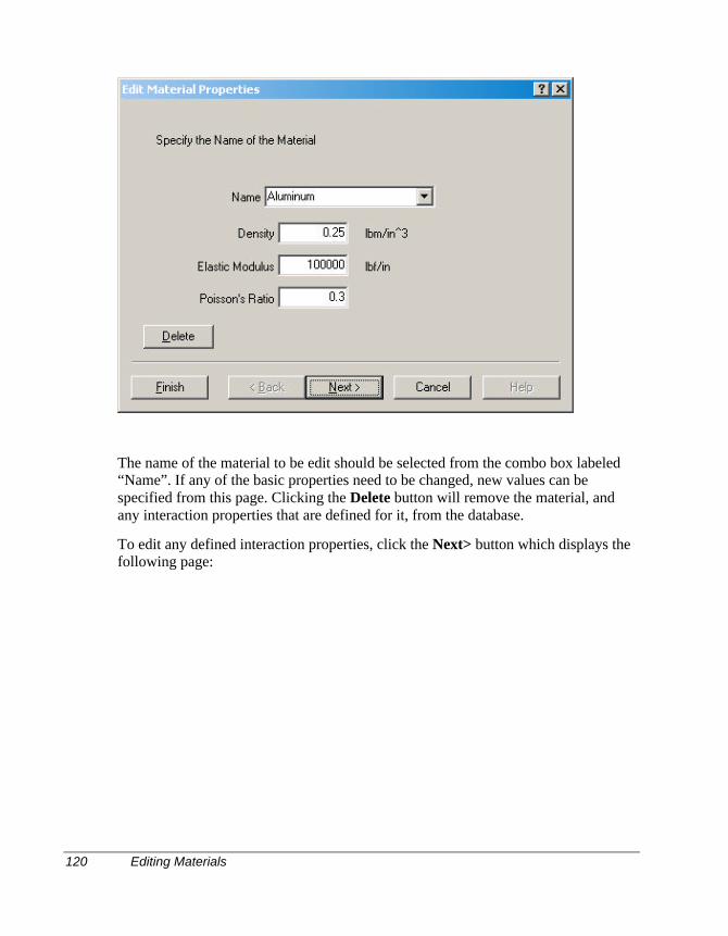
120 Editing Materials
The name of the material to be edit should be selected from the combo box labeled“Name”. If any of the basic properties need to be changed, new values can bespecified from this page. Clicking the Delete button will remove the material, andany interaction properties that are defined for it, from the database.
To edit any defined interaction properties, click the Next> button which displays thefollowing page:
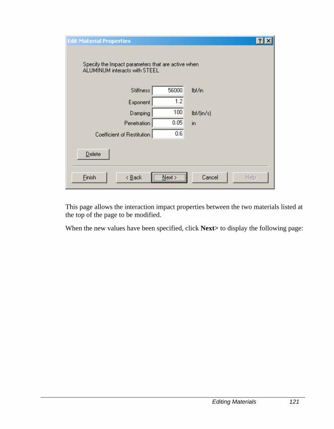
Editing Materials 121
This page allows the interaction impact properties between the two materials listed atthe top of the page to be modified.
When the new values have been specified, click Next> to display the following page:
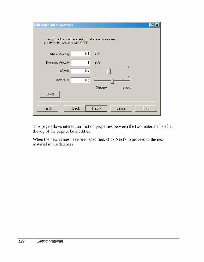
122 Editing Materials
This page allows interaction friction properties between the two materials listed atthe top of the page to be modified.
When the new values have been specified, click Next> to proceed to the nextmaterial in the database.
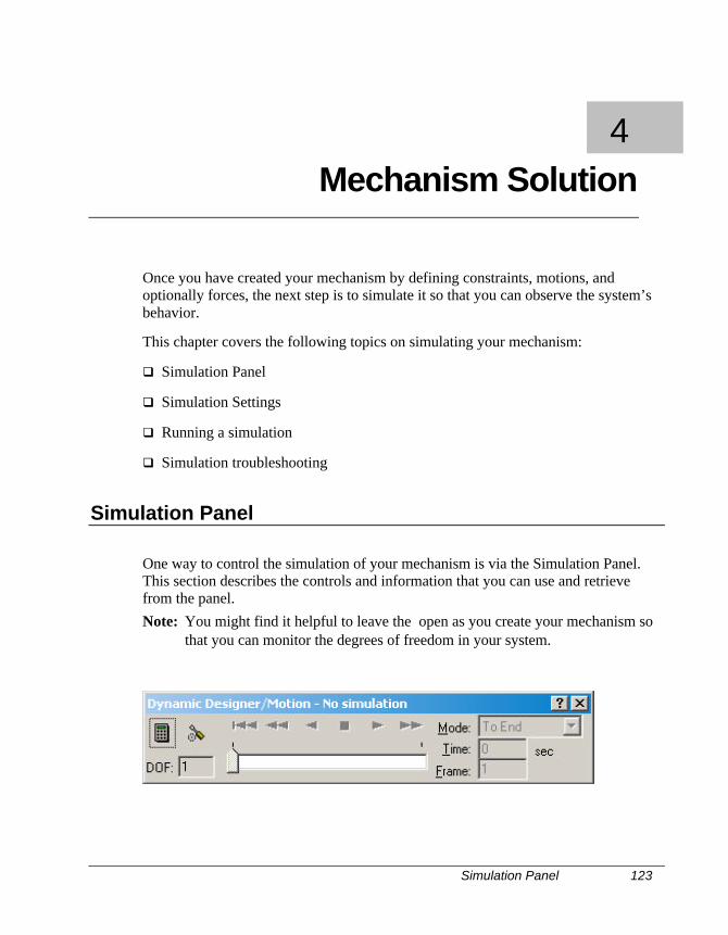
Simulation Panel 123
Once you have created your mechanism by defining constraints, motions, andoptionally forces, the next step is to simulate it so that you can observe the system’sbehavior.
This chapter covers the following topics on simulating your mechanism:
q Simulation Panel
q Simulation Settings
q Running a simulation
q Simulation troubleshooting
Simulation Panel
One way to control the simulation of your mechanism is via the Simulation Panel.This section describes the controls and information that you can use and retrievefrom the panel.Note: You might find it helpful to leave the open as you create your mechanism so
that you can monitor the degrees of freedom in your system.
4 Mechanism Solution
124 Simulation Panel
Status
The status message line in the title of the indicates the status of your mechanism. Itdisplays one of the following messages:
q No Active Mechanism - You do not have an open mechanism file.
q No Simulation - You have an active mechanism, but have not simulated it.
q Simulating... - Displayed when a simulation is running. Indicates the currentsimulation time and frame number.
q Simulated... - Displayed after a simulation has run and indicates the totalsimulation time and total number of frames [Example: Simulated 1 sec, 50frames].
q Aborted - Indicates that the simulation ended abnormally before the end of thesimulation time specified was reached.
DOF Counter
The automatic DOF counter in the lower left corner of the Simulation Panel keeps arunning total of the degrees of freedom in your system. This count refers to the actualdegrees of freedom in the system after the removal of redundant constraints.
Button Controls and Scroll Bar
The arrow buttons on the Simulation Panel are the animation playback controls.These buttons are, from left to right, Mechanism Reset, Fast Reverse, Reverse Play,Stop, Forward Play, and Fast Forward. The Mechanism Reset button can be used toreset the mechanism to its original configuration after a simulation or animation. Youcan also reset the mechanism by clicking Motion, Reset. Once the simulation hasbeen started, the Stop button can be used to end the simulation. The other buttons canbe used to animate the mechanism only after a simulation is run.
You can drag the scroll bar to move the mechanism to any frame in the simulation.
The animation playback controls are discussed in more detail in the followingchapter “Reviewing Your Results”.
Mode
The Mode option list controls the animation mode. You can set the mode to:
q To End - The animation plays one time either forwards or backwards and stops.
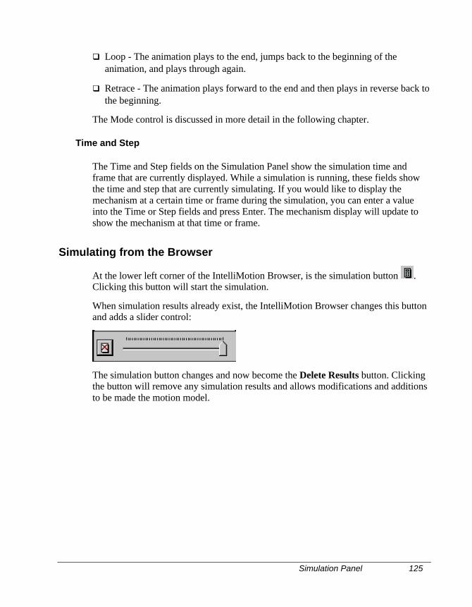
Simulation Panel 125
q Loop - The animation plays to the end, jumps back to the beginning of theanimation, and plays through again.
q Retrace - The animation plays forward to the end and then plays in reverse back tothe beginning.
The Mode control is discussed in more detail in the following chapter.
Time and Step
The Time and Step fields on the Simulation Panel show the simulation time andframe that are currently displayed. While a simulation is running, these fields showthe time and step that are currently simulating. If you would like to display themechanism at a certain time or frame during the simulation, you can enter a valueinto the Time or Step fields and press Enter. The mechanism display will update toshow the mechanism at that time or frame.
Simulating from the Browser
At the lower left corner of the IntelliMotion Browser, is the simulation button .Clicking this button will start the simulation.
When simulation results already exist, the IntelliMotion Browser changes this buttonand adds a slider control:
The simulation button changes and now become the Delete Results button. Clickingthe button will remove any simulation results and allows modifications and additionsto be made the motion model.
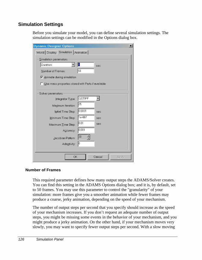
126 Simulation Panel
Simulation Settings
Before you simulate your model, you can define several simulation settings. Thesimulation settings can be modified in the Options dialog box.
Number of Frames
This required parameter defines how many output steps the ADAMS/Solver creates.You can find this setting in the ADAMS Options dialog box; and it is, by default, setto 50 frames. You may use this parameter to control the "granularity" of yoursimulation: more frames give you a smoother animation while fewer frames mayproduce a coarse, jerky animation, depending on the speed of your mechanism.
The number of output steps per second that you specify should increase as the speedof your mechanism increases. If you don’t request an adequate number of outputsteps, you might be missing some events in the behavior of your mechanism, and youmight produce a jerky animation. On the other hand, if your mechanism moves veryslowly, you may want to specify fewer output steps per second. With a slow moving
Simulation Panel 127
mechanism, a large number of output steps per second may be unnecessary becauseevents are happening more slowly.Note: The number in the Number of Frames field is the total number of output steps
for your simulation, not the number of output steps per second.Note: Do not confuse the speed at which the mechanism moves with the animation
rate! A mechanism’s speed is based on how fast its components are moving orchanging direction. The animation rate is the number of frames per secondthat are displayed and is dependent on your computer hardware.
Duration or Time Increment
This is a required parameter that specifies the length of time for a simulation or thetime increment for each output step. You can find this setting in the SimulationOptions dialog box; and it is, by default, set to 1 second. Note that the beginning timefor a simulation is always time=0. A logical ending time is the time required for themechanism to complete one cycle. However, you may use this parameter to focus ona particular ending time for your simulation. For example, you may have a robot armthat extends and retracts. If you are only examining the extension of the arm, youcould set the simulation duration to the point where the arm is fully extended.
Animate during simulation
You can find the Animate during simulation button on the Simulate panel in theADAMS Options dialog box. If you turn on the Animate during simulation setting,the mechanism animates as the simulation runs. If this setting is off, the simulationruns and the mechanism remains in its assembled position. Animating during asimulation provides instant feedback to you as your simulation runs.
Use mass properties stored with parts
If this option is checked, Dynamic Designer will use the last mass properties values itmaintains for the parts during the simulation. If this box is cleared, DynamicDesigner will recalculate all part mass properties prior to running the simulation. Usethis option if you have a large model that has not had any geometric modificationsmade recently. It will significantly increase performance. A good strategy is to leavethis box cleared for the first simulation, and then check it for subsequent simulationas long as no geometric modifications have been made to any of the parts in themotion model that may have changed their mass properties.
Solver Parameters
The values listed in the Solver Parameters group are used to control the operation ofthe ADAMS/Solver. These parameters are explained below:
128 Simulation Panel
Integrator Type
ADAMS/Solver supports two integrator types. GSTIFF is the default and is fasterand, in certain circumstances, slightly less accurate than the WSTIFF integrator.
Maximum Iterations
The “Maximum Iterations” parameter specifies the maximum number of times thenumeric integrator iterates in the search for a solution for a given time step. If theSolver exceeds this limit, a convergence failure is recorded. The Solver will thenquarter the last time step taken and integrate again. If four consecutive failures arerecorded, the Solver stops with information on the probable cause. The default is 4and should usually not be changed.
Initial Time Step
The “Initial Time Step” is useful to get the Solver started more quickly. It is the firststep size used by the variable step integrator. If it results in a convergence error to begreater than one, a very conservative first step size is estimated by the solver.Resetting “Initial Time Step” to a less conservative value could get the solver startedfaster in subsequent runs of the model or slight variation of it.
Maximum Time Step
The “Maximum Time Step” should be large and is usually of little concern unless thesolver is missing some short lived events like impacts. Then “Maximum Time Step”should be set to the same order as the short lived events. Integration time can bemuch longer because the Solver cannot move forward as fast.
Minimum Time Step
The “Minimum Time Step” should be small and is usually of little concern unless themodel has a locked position which the Solver is trying to locate to a very highprecision needlessly. Setting the parameter to a larger value will cause the solver tostop sooner once a locked position is found.
Accuracy
The “Accuracy” parameter specifies the criteria that is used to determine when thesolution for the time step has converged. Larger value will cause the solver to runfaster, but produce more “sloppy” results. Smaller values cause the solver to takelonger, but result in more accurate results. The default value chosen is a good
Simulating 129
compromise for most problems.
Jacobian Pattern
The “Jacobian Pattern” parameter controls how often the simulation engine’sjacobian matrix is updated. The value is in percent. At 100%, the jacobian is updatedat every integration time step. At 50% the jacobian is updated every otherintegration time step. This value impacts models that contain intermittent curve/curvecontact. The higher the value the better from an accuracy standpoint, but the higherthe value, the more impact in the overall simulation time.
Adaptivity
The “Adaptivity” parameter is also used primarily for intermittent curve/curveproblems. If problems occur where contacts are not detected, this value can beprogressively decreased. A good starting point is 10e-6, with reductions of 10e-1.
Simulating
This section describes how to perform a simulation.
To perform a simulation:
1 Click the Browser Simulate button , or if you would like to use the SimulationPanel, open it by selecting the button on the Motion Toolbar.
The Simulation Panel appears. If you have not already simulated yourmechanism, the title bar should read “No Simulation.”
2 If you would like to modify the Number of Frames or the Duration/TimeIncrement settings, click the Options button on the Simulation Panel,directly above the DOF counter.
The ADAMS Options dialog box appears.
3 Click the Simulate tab.
4 You can modify the Number of Frames, Duration/Time Increment, orAnimate during simulation settings.
5 Click OK to complete the settings modification and close the ADAMS Optionsdialog box.
130 Simulation Troubleshooting
6 Click the Simulate button on the Simulation Panel to begin the simulation.
If you toggled off the Animate during simulation setting, the scroll bar on thetoolbar advances as the simulation advances. Also the Time and Step fields showthe current simulation time and frame. If the Animate during simulation toggleis on, the mechanism animates as the simulation advances.
7 After the simulation is complete, you can click the Forward Play, Reverse Play,Fast Forward, Fast Rewind, or Reset buttons to animate or reset the mechanism.
Simulation Troubleshooting
The following are frequently asked simulation questions and answers.
1 Q: The reaction forces in the joints that are calculated are incorrect by quite a bit,over a factor of ten. What might I be doing wrong?
A: First check that you have properly set the units of your mechanism. Also checkthat you have properly set the density of each of your components. To check thedensity of a component, select Tools, Options and then select the MaterialProperties tab while viewing the component (not the assembly). Incorrectsettings of units or density can affect the reaction forces significantly.
2 Q: The standard (built-in) animation runs slowly on my PC. Is there a way to getfast, shaded animation?
A: Yes. You can save mechanism animation to an “.AVI” file. See “Exporting an.AVI movie” on page 134 for more information.
3 Q: How do I get a plot of my output data?
A: You can export your output data to Excel or to a text file. See ExportingResults to Excel on page 137 or Exporting Results to a Text File on page 140 formore information.
Animating The Mechanism 131
After you have simulated your mechanism, you can review the results in severalways. You can play animations or review the numerical data and plots in Excel.Animations can also be exported to AVI movies and VRML format. This chapterdescribes the following:
q Animating in Solid Edge
q Exporting animations to AVI movies
q Exporting animations to VRML
q Exporting results to Excel
q Exporting results to a text file
q Interference Detection
q Exporting Force results to FEA
Animating The Mechanism
Animation of a software prototype of a mechanism can help you predict themechanism’s behavior and refine its design prior to manufacturing. You can animateyour mechanism during or immediately following a simulation.
One frame of animation is created for each output step.
Playback Controls
The animation playback controls are located on the Simulation Panel, and are alsoexplained in the previous chapter.
These buttons are, from left to right:
5 Reviewing Your Results
132 Animating The Mechanism
q Mechanism Reset - Resets the mechanism to its original configuration after asimulation or animation.
q Fast Rewind - Plays the mechanism in the reverse direction but skips frames sothat the animation is faster than regular play. You can control the number ofskipped frames in the ADAMS Options dialog box.
q Reverse Play - Plays every frame of the animation in the reverse direction.
q Stop - Stops a simulation or animation.
q Forward Play - Plays every frame of the animation in the forward direction.
q Fast Forward - Plays the animation in the forward direction, skipping frames sothat the animation is faster than Forward Play. You can control the number ofskipped frames in the ADAMS Options dialog box.
As mentioned above, the Mechanism Reset button resets the mechanism to itsoriginal configuration. You can also reset the mechanism by clicking Motion, Reset.Once a simulation has been started, the Stop button can be used to end thesimulation. The Stop button also stops an animation. The other buttons can be used toanimate the mechanism only after a simulation or portion of a simulation is run.
You can drag the scroll bar to move the mechanism to any frame in the simulation.
Mode
The Mode option list controls the animation mode. You can set the mode to:
q To End - The animation plays one time either forwards or backwards and stops.
q Loop - The animation plays to the end, jumps back to the beginning of theanimation, and plays through again. The animation plays until you press the Stopbutton.
q Retrace - The animation plays forward to the end and then plays in reverse back tothe beginning. The animation plays until you press the Stop button.
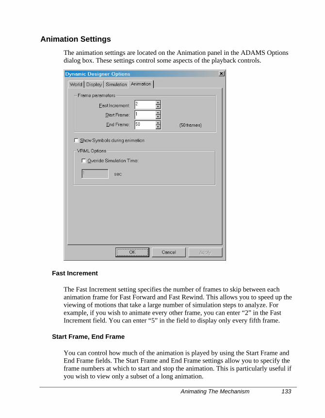
Animating The Mechanism 133
Animation Settings
The animation settings are located on the Animation panel in the ADAMS Optionsdialog box. These settings control some aspects of the playback controls.
Fast Increment
The Fast Increment setting specifies the number of frames to skip between eachanimation frame for Fast Forward and Fast Rewind. This allows you to speed up theviewing of motions that take a large number of simulation steps to analyze. Forexample, if you wish to animate every other frame, you can enter “2” in the FastIncrement field. You can enter “5” in the field to display only every fifth frame.
Start Frame, End Frame
You can control how much of the animation is played by using the Start Frame andEnd Frame fields. The Start Frame and End Frame settings allow you to specify theframe numbers at which to start and stop the animation. This is particularly useful ifyou wish to view only a subset of a long animation.
134 Exporting an AVI movie
The first frame always shows the mechanism in its assembled state, and the secondframe is the first frame of the animation. The last frame is therefore numbered 1greater than the number of steps in the simulation. For example, if you perform asimulation with 10 output steps, the frames are numbered from 1 to 11.
Show Symbols during animation
When this option is checked, Dynamic Designer Motion object symbols are shownduring animation. When this option is clear, the symbols are not displayed.
Animating a Simulation
In order to animate a mechanism, you must first simulate it. Nearly all of thesimulation and animation controls are located on the Simulation Panel. The othersimulation and animation settings can be found on the ADAMS Options dialog box.
To animate a mechanism:
1 If the Simulation Panel is not open, click Motion, Toolbar.
2 Simulate the mechanism by clicking the calculator icon on the upper left cornerof the toolbar.
See Chapter 5, “Simulating a Mechanism” for more information on simulating.
3 After the simulation has finished, press any of the arrow buttons to animate themechanism forward, backward, fast forward, or fast rewind. Press the stop buttonto stop an animation or a simulation.
4 If you would like to change the animation settings, open the Options dialog boxby clicking the options icon on the Toolbar, which is directly above the Degreeof Freedom Counter.
5 Click the Animation tab.
6 Modify any of the animation settings and click OK to close the dialog box.
7 You can continue to animate your mechanism by pressing the arrow buttons.
Exporting an AVI movie
If the animations run slowly on your PC, you can create faster animations byconverting them into AVI movies.
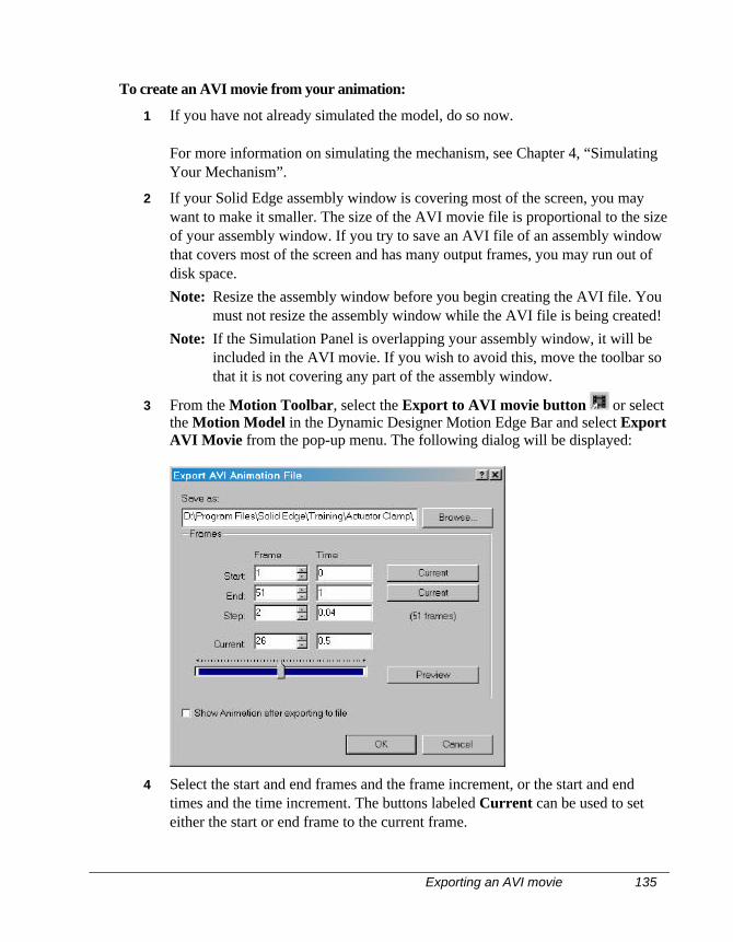
Exporting an AVI movie 135
To create an AVI movie from your animation:
1 If you have not already simulated the model, do so now.
For more information on simulating the mechanism, see Chapter 4, “SimulatingYour Mechanism”.
2 If your Solid Edge assembly window is covering most of the screen, you maywant to make it smaller. The size of the AVI movie file is proportional to the sizeof your assembly window. If you try to save an AVI file of an assembly windowthat covers most of the screen and has many output frames, you may run out ofdisk space.Note: Resize the assembly window before you begin creating the AVI file. You
must not resize the assembly window while the AVI file is being created!Note: If the Simulation Panel is overlapping your assembly window, it will be
included in the AVI movie. If you wish to avoid this, move the toolbar sothat it is not covering any part of the assembly window.
3 From the Motion Toolbar, select the Export to AVI movie button or selectthe Motion Model in the Dynamic Designer Motion Edge Bar and select ExportAVI Movie from the pop-up menu. The following dialog will be displayed:
4 Select the start and end frames and the frame increment, or the start and endtimes and the time increment. The buttons labeled Current can be used to seteither the start or end frame to the current frame.
136 Exporting Animations to VRML
The Preview button will display the frames that will be included in theanimation. The Show Animation after exporting to file will replay theanimation after it has been generated.
5 Click OK.
The mechanism animates through its range of motion as the AVI movie iscreated.
Exporting Animations to VRML
If you would like to place your animation on your website or your intranet, you caneasily export your animations in VRML format. You can download a plug-in foryour Web browser called Cosmo Player to view VRML files. This plug-in can bedownloaded from: http://cosmo.sgi.com/.
Before exporting the animation, you may need to modify the animation duration forthe VRML movie. The default animation duration is the simulation time. The CosmoPlayer will attempt to squeeze the animation into the simulation time and may skipframes as a result. You can avoid this situation by modifying the Override SimulationTime setting in the ADAMS Options dialog box.
To Export an Animation to VRML:
1 On the Motion Toolbar, click on the Options button .
2 Click the Animation tab.
3 On the Animation panel, toggle on the Override Simulation Time setting.
4 Set the Animation Time so that the animation will run smoothly withoutskipping frames. For example, for an animation with 50 frames, you shouldprobably set the Animation Time to approximately 10-15 seconds.
5 Click OK.
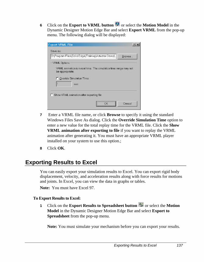
Exporting Results to Excel 137
6 Click on the Export to VRML button or select the Motion Model in theDynamic Designer Motion Edge Bar and select Export VRML from the pop-upmenu. The following dialog will be displayed:
7 Enter a VRML file name, or click Browse to specify it using the standardWindows Files Save As dialog. Click the Override Simulation Time option toenter a new value for the total replay time for the VRML file. Click the ShowVRML animation after exporting to file if you want to replay the VRMLanimation after generating it. You must have an appropriate VRML playerinstalled on your system to use this option.;
8 Click OK.
Exporting Results to Excel
You can easily export your simulation results to Excel. You can export rigid bodydisplacement, velocity, and acceleration results along with force results for motionsand joints. In Excel, you can view the data in graphs or tables.Note: You must have Excel 97.
To Export Results to Excel:
1 Click on the Export Results to Spreadsheet button or select the MotionModel in the Dynamic Designer Motion Edge Bar and select Export toSpreadsheet from the pop-up menu.
Note: You must simulate your mechanism before you can export your results.
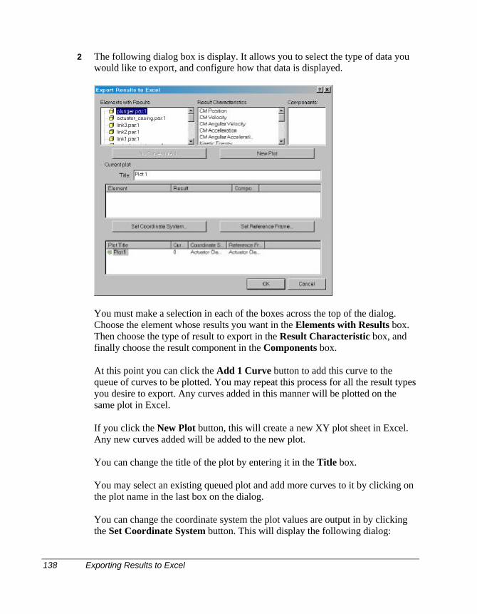
138 Exporting Results to Excel
2 The following dialog box is display. It allows you to select the type of data youwould like to export, and configure how that data is displayed.
You must make a selection in each of the boxes across the top of the dialog.Choose the element whose results you want in the Elements with Results box.Then choose the type of result to export in the Result Characteristic box, andfinally choose the result component in the Components box.
At this point you can click the Add 1 Curve button to add this curve to thequeue of curves to be plotted. You may repeat this process for all the result typesyou desire to export. Any curves added in this manner will be plotted on thesame plot in Excel.
If you click the New Plot button, this will create a new XY plot sheet in Excel.Any new curves added will be added to the new plot.
You can change the title of the plot by entering it in the Title box.
You may select an existing queued plot and add more curves to it by clicking onthe plot name in the last box on the dialog.
You can change the coordinate system the plot values are output in by clickingthe Set Coordinate System button. This will display the following dialog:
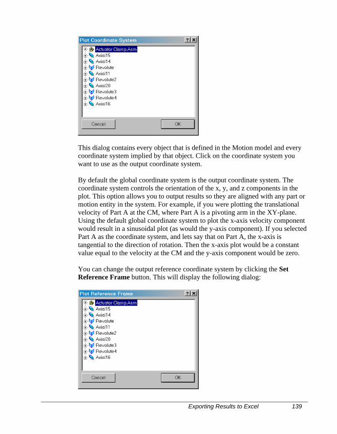
Exporting Results to Excel 139
This dialog contains every object that is defined in the Motion model and everycoordinate system implied by that object. Click on the coordinate system youwant to use as the output coordinate system.
By default the global coordinate system is the output coordinate system. Thecoordinate system controls the orientation of the x, y, and z components in theplot. This option allows you to output results so they are aligned with any part ormotion entity in the system. For example, if you were plotting the translationalvelocity of Part A at the CM, where Part A is a pivoting arm in the XY-plane.Using the default global coordinate system to plot the x-axis velocity componentwould result in a sinusoidal plot (as would the y-axis component). If you selectedPart A as the coordinate system, and lets say that on Part A, the x-axis istangential to the direction of rotation. Then the x-axis plot would be a constantvalue equal to the velocity at the CM and the y-axis component would be zero.
You can change the output reference coordinate system by clicking the SetReference Frame button. This will display the following dialog:

140 Exporting Results to a Text File
This dialog contains every object that is defined in the Motion model and everycoordinate system implied by that object. Click on the coordinate system youwant to use as the reference coordinate system.
By default the global coordinate system is the reference coordinate system. Thereference frame determines the relative system the result is measured withrespect to. For example, if you selected to plot the velocity of partA, and youselected partB as the reference frame, you would be measuring the relativevelocity of partA with respect to partB.
You can delete a queued curve or plot by selecting it in the appropriate box andpressing the DELETE key.
3 When all the curves and plots have been specified, Click OK to actually createthe plots in Excel.
Dynamic Designer/Motion automatically creates an Excel worksheet with graphsand tables for each of the elements that you selected.
Exporting Results to a Text File
You can export your simulation results to a text file in case you would like to reviewthe results in another format. For example, if you do not have Excel 97, you can stillexport you results and read them into your favorite spreadsheet tool.
To Export Results to Text File:
1 Click Motion, Export Results, To File...
2 Enter a file name.
3 Click OK.Dynamic Designer/Motion automatically create a text file that contains all of theresults for each of the entities in your simulation. If you read the file into aspreadsheet, the text is space delimited.
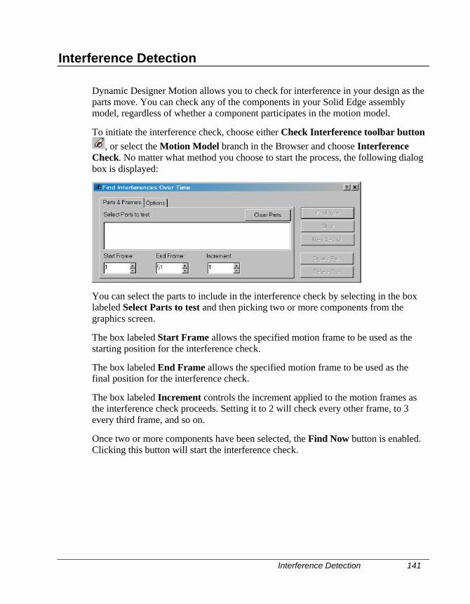
Interference Detection 141
Interference Detection
Dynamic Designer Motion allows you to check for interference in your design as theparts move. You can check any of the components in your Solid Edge assemblymodel, regardless of whether a component participates in the motion model.
To initiate the interference check, choose either Check Interference toolbar button, or select the Motion Model branch in the Browser and choose Interference
Check. No matter what method you choose to start the process, the following dialogbox is displayed:
You can select the parts to include in the interference check by selecting in the boxlabeled Select Parts to test and then picking two or more components from thegraphics screen.
The box labeled Start Frame allows the specified motion frame to be used as thestarting position for the interference check.
The box labeled End Frame allows the specified motion frame to be used as thefinal position for the interference check.
The box labeled Increment controls the increment applied to the motion frames asthe interference check proceeds. Setting it to 2 will check every other frame, to 3every third frame, and so on.
Once two or more components have been selected, the Find Now button is enabled.Clicking this button will start the interference check.
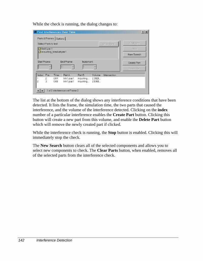
142 Interference Detection
While the check is running, the dialog changes to:
The list at the bottom of the dialog shows any interference conditions that have beendetected. It lists the frame, the simulation time, the two parts that caused theinterference, and the volume of the interference detected. Clicking on the indexnumber of a particular interference enables the Create Part button. Clicking thisbutton will create a new part from this volume, and enable the Delete Part buttonwhich will remove the newly created part if clicked.
While the interference check is running, the Stop button is enabled. Clicking this willimmediately stop the check.
The New Search button clears all of the selected components and allows you toselect new components to check. The Clear Parts button, when enabled, removes allof the selected parts from the interference check.
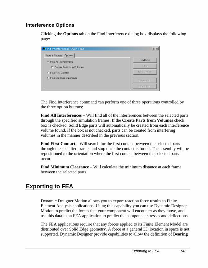
Exporting to FEA 143
Interference Options
Clicking the Options tab on the Find Interference dialog box displays the followingpage:
The Find Interference command can perform one of three operations controlled bythe three option buttons:
Find All Interferences – Will find all of the interferences between the selected partsthrough the specified simulation frames. If the Create Parts from Volumes checkbox is checked, Solid Edge parts will automatically be created from each interferencevolume found. If the box is not checked, parts can be created from interferingvolumes in the manner described in the previous section.
Find First Contact – Will search for the first contact between the selected partsthrough the specified frame, and stop once the contact is found. The assembly will berepositioned to the orientation where the first contact between the selected partsoccur.
Find Minimum Clearance – Will calculate the minimum distance at each framebetween the selected parts.
Exporting to FEA
Dynamic Designer Motion allows you to export reaction force results to FiniteElement Analysis applications. Using this capability you can use Dynamic DesignerMotion to predict the forces that your component will encounter as they move, anduse this data in an FEA application to predict the component stresses and deflections.
The FEA applications require that any forces applied to its Finite Element Model aredistributed over Solid Edge geometry. A force at a general 3D location in space is notsupported. Dynamic Designer provide capabilities to allow the definition of Bearing
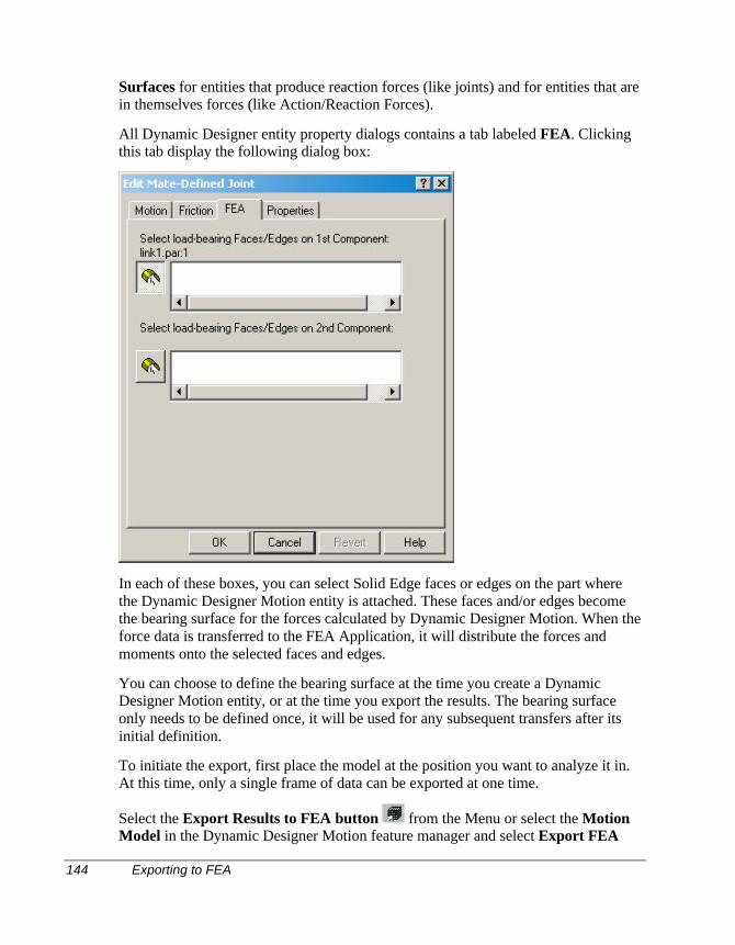
144 Exporting to FEA
Surfaces for entities that produce reaction forces (like joints) and for entities that arein themselves forces (like Action/Reaction Forces).
All Dynamic Designer entity property dialogs contains a tab labeled FEA. Clickingthis tab display the following dialog box:
In each of these boxes, you can select Solid Edge faces or edges on the part wherethe Dynamic Designer Motion entity is attached. These faces and/or edges becomethe bearing surface for the forces calculated by Dynamic Designer Motion. When theforce data is transferred to the FEA Application, it will distribute the forces andmoments onto the selected faces and edges.
You can choose to define the bearing surface at the time you create a DynamicDesigner Motion entity, or at the time you export the results. The bearing surfaceonly needs to be defined once, it will be used for any subsequent transfers after itsinitial definition.
To initiate the export, first place the model at the position you want to analyze it in.At this time, only a single frame of data can be exported at one time.
Select the Export Results to FEA button from the Menu or select the MotionModel in the Dynamic Designer Motion feature manager and select Export FEA
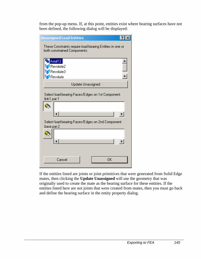
Exporting to FEA 145
from the pop-up menu. If, at this point, entities exist where bearing surfaces have notbeen defined, the following dialog will be displayed:
If the entities listed are joints or joint primitives that were generated from Solid Edgemates, then clicking the Update Unassigned will use the geometry that wasoriginally used to create the mate as the bearing surface for these entities. If theentities listed here are not joints that were created from mates, then you must go backand define the bearing surface in the entity property dialog.
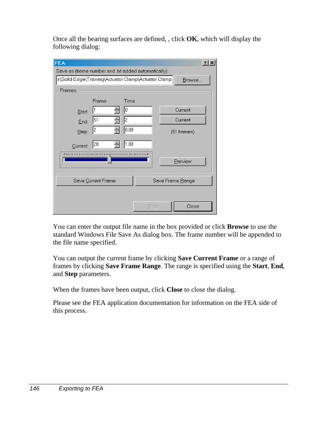
146 Exporting to FEA
Once all the bearing surfaces are defined, , click OK, which will display thefollowing dialog:
You can enter the output file name in the box provided or click Browse to use thestandard Windows File Save As dialog box. The frame number will be appended tothe file name specified.
You can output the current frame by clicking Save Current Frame or a range offrames by clicking Save Frame Range. The range is specified using the Start, End,and Step parameters.
When the frames have been output, click Close to close the dialog.
Please see the FEA application documentation for information on the FEA side ofthis process.
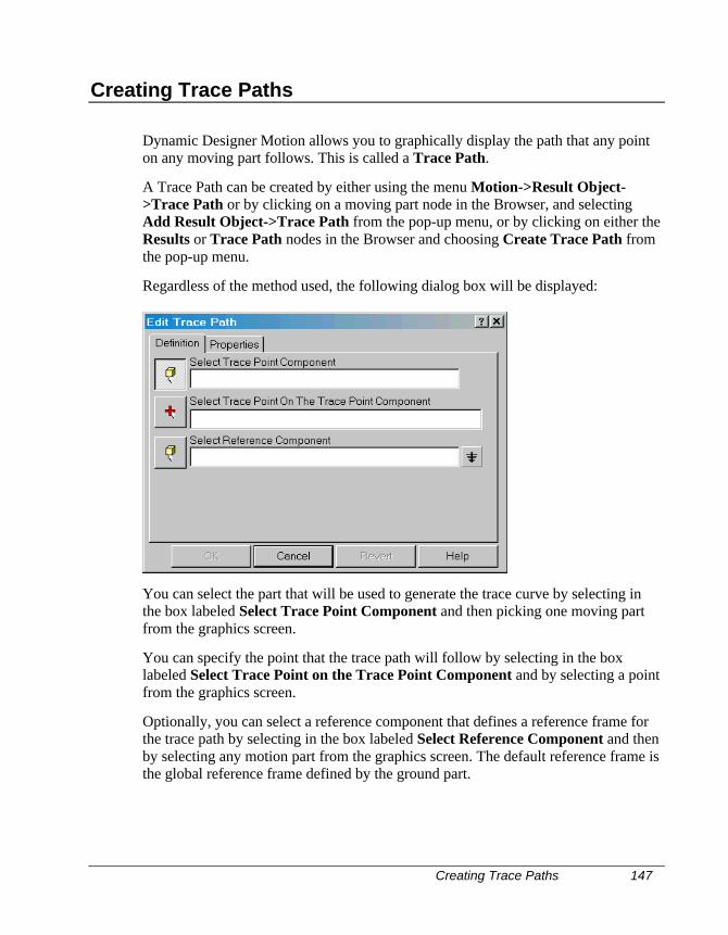
Creating Trace Paths 147
Creating Trace Paths
Dynamic Designer Motion allows you to graphically display the path that any pointon any moving part follows. This is called a Trace Path.
A Trace Path can be created by either using the menu Motion->Result Object->Trace Path or by clicking on a moving part node in the Browser, and selectingAdd Result Object->Trace Path from the pop-up menu, or by clicking on either theResults or Trace Path nodes in the Browser and choosing Create Trace Path fromthe pop-up menu.
Regardless of the method used, the following dialog box will be displayed:
You can select the part that will be used to generate the trace curve by selecting inthe box labeled Select Trace Point Component and then picking one moving partfrom the graphics screen.
You can specify the point that the trace path will follow by selecting in the boxlabeled Select Trace Point on the Trace Point Component and by selecting a pointfrom the graphics screen.
Optionally, you can select a reference component that defines a reference frame forthe trace path by selecting in the box labeled Select Reference Component and thenby selecting any motion part from the graphics screen. The default reference frame isthe global reference frame defined by the ground part.
148 Exporting Trace Paths Points
Exporting Trace Paths Points
The 3D coordinate values that define a trace path can be export to a comma separatedvalue (CSV) formatted file which can then be imported to a spreadsheet program likeMicrosoft Excel.
To export the values, click on the trace path(s) whose coordinates are to be exported,and choose Export CSV from the pop-up menu. The standard Windows File SaveAs dialog box will be displayed requesting the name of the CSV file to be created.
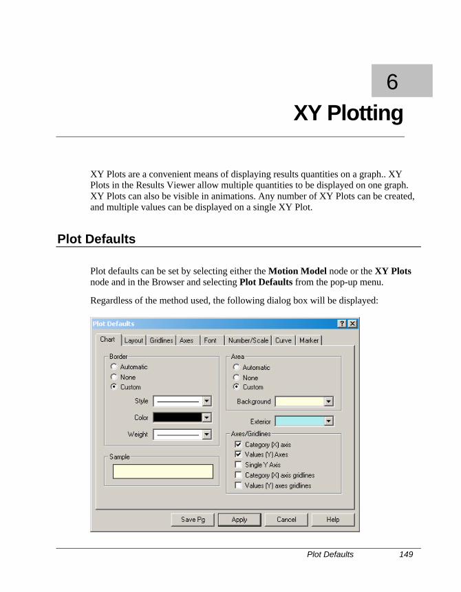
Plot Defaults 149
XY Plots are a convenient means of displaying results quantities on a graph.. XYPlots in the Results Viewer allow multiple quantities to be displayed on one graph.XY Plots can also be visible in animations. Any number of XY Plots can be created,and multiple values can be displayed on a single XY Plot.
Plot Defaults
Plot defaults can be set by selecting either the Motion Model node or the XY Plotsnode and in the Browser and selecting Plot Defaults from the pop-up menu.
Regardless of the method used, the following dialog box will be displayed:
6 XY Plotting
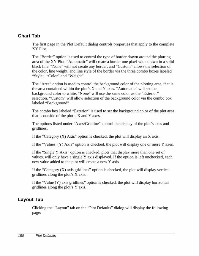
150 Plot Defaults
Chart Tab
The first page in the Plot Default dialog controls properties that apply to the completeXY Plot.
The “Border” option is used to control the type of border drawn around the plottingarea of the XY Plot. “Automatic” will create a border one pixel wide drawn in a solidblack line. “None” will not create any border, and “Custom” allows the selection ofthe color, line weight, and line style of the border via the three combo boxes labeled“Style”, “Color” and “Weight”.
The “Area” option is used to control the background color of the plotting area, that isthe area contained within the plot’s X and Y axes. “Automatic” will set thebackground color to white. “None” will use the same color as the “Exterior”selection. “Custom” will allow selection of the background color via the combo boxlabeled “Background”.
The combo box labeled “Exterior” is used to set the background color of the plot areathat is outside of the plot’s X and Y axes.
The options listed under “Axes/Gridline” control the display of the plot’s axes andgridlines.
If the “Category (X) Axis” option is checked, the plot will display an X axis.
If the “Values (Y) Axis” option is checked, the plot will display one or more Y axes.
If the “Single Y Axis” option is checked, plots that display more than one set ofvalues, will only have a single Y axis displayed. If the option is left unchecked, eachnew value added to the plot will create a new Y axis.
If the “Category (X) axis gridlines” option is checked, the plot will display verticalgridlines along the plot’s X axis.
If the “Value (Y) axis gridlines” option is checked, the plot will display horizontalgridlines along the plot’s Y axis.
Layout Tab
Clicking the “Layout” tab on the “Plot Defaults” dialog will display the followingpage:
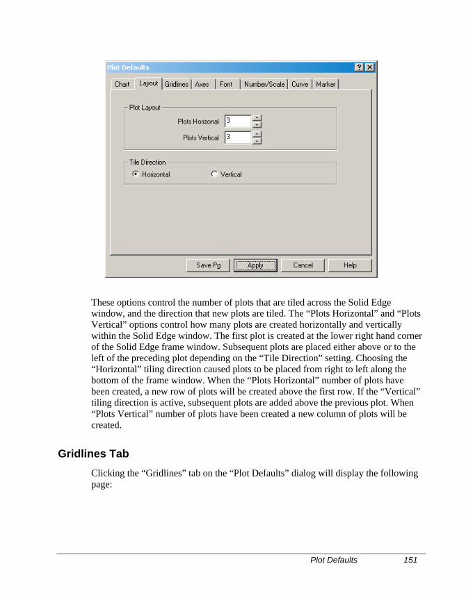
Plot Defaults 151
These options control the number of plots that are tiled across the Solid Edgewindow, and the direction that new plots are tiled. The “Plots Horizontal” and “PlotsVertical” options control how many plots are created horizontally and verticallywithin the Solid Edge window. The first plot is created at the lower right hand cornerof the Solid Edge frame window. Subsequent plots are placed either above or to theleft of the preceding plot depending on the “Tile Direction” setting. Choosing the“Horizontal” tiling direction caused plots to be placed from right to left along thebottom of the frame window. When the “Plots Horizontal” number of plots havebeen created, a new row of plots will be created above the first row. If the “Vertical”tiling direction is active, subsequent plots are added above the previous plot. When“Plots Vertical” number of plots have been created a new column of plots will becreated.
Gridlines Tab
Clicking the “Gridlines” tab on the “Plot Defaults” dialog will display the followingpage:
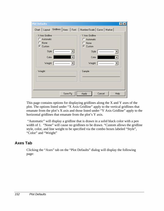
152 Plot Defaults
This page contains options for displaying gridlines along the X and Y axes of theplot. The options listed under “X Axis Gridline” apply to the vertical gridlines thatemanate from the plot’s X axis and those listed under “Y Axis Gridline” apply to thehorizontal gridlines that emanate from the plot’s Y axis.
“Automatic” will display a gridline that is drawn in a solid black color with a penwidth of 1. “None” will cause no gridlines to be drawn. “Custom allows the gridlinestyle, color, and line weight to be specified via the combo boxes labeled “Style”,“Color” and “Weight”
Axes Tab
Clicking the “Axes” tab on the “Plot Defaults” dialog will display the followingpage:
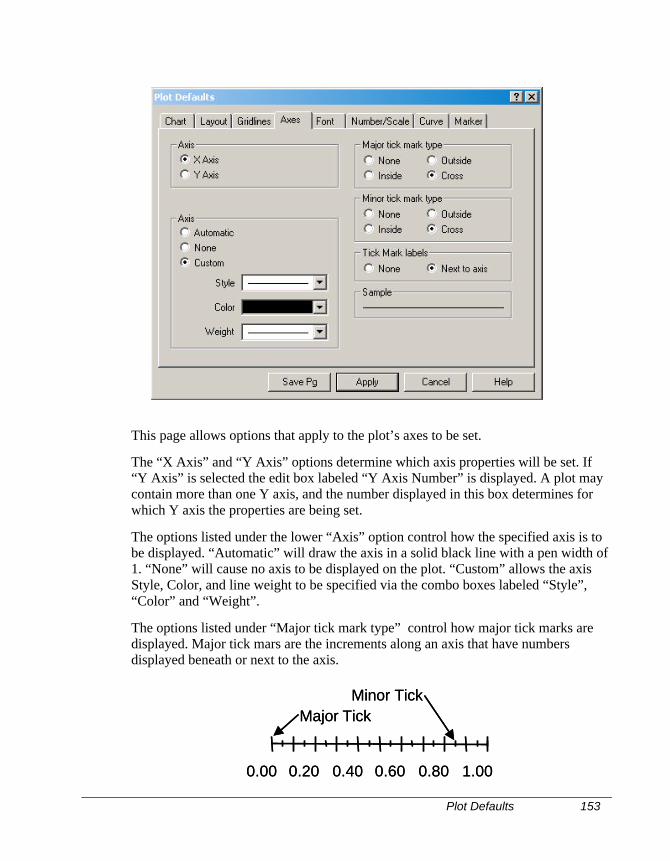
Plot Defaults 153
This page allows options that apply to the plot’s axes to be set.
The “X Axis” and “Y Axis” options determine which axis properties will be set. If“Y Axis” is selected the edit box labeled “Y Axis Number” is displayed. A plot maycontain more than one Y axis, and the number displayed in this box determines forwhich Y axis the properties are being set.
The options listed under the lower “Axis” option control how the specified axis is tobe displayed. “Automatic” will draw the axis in a solid black line with a pen width of1. “None” will cause no axis to be displayed on the plot. “Custom” allows the axisStyle, Color, and line weight to be specified via the combo boxes labeled “Style”,“Color” and “Weight”.
The options listed under “Major tick mark type” control how major tick marks aredisplayed. Major tick mars are the increments along an axis that have numbersdisplayed beneath or next to the axis.
0.00 0.20 0.40 0.60 0.80 1.00
Major TickMinor Tick
0.00 0.20 0.40 0.60 0.80 1.00
Major TickMinor Tick
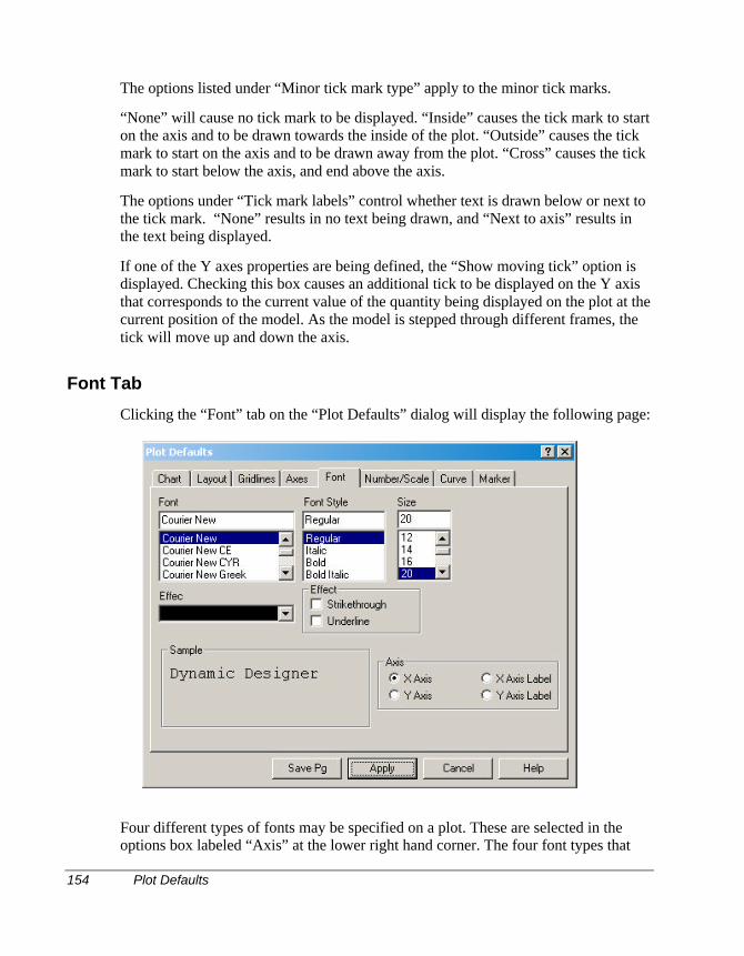
154 Plot Defaults
The options listed under “Minor tick mark type” apply to the minor tick marks.
“None” will cause no tick mark to be displayed. “Inside” causes the tick mark to starton the axis and to be drawn towards the inside of the plot. “Outside” causes the tickmark to start on the axis and to be drawn away from the plot. “Cross” causes the tickmark to start below the axis, and end above the axis.
The options under “Tick mark labels” control whether text is drawn below or next tothe tick mark. “None” results in no text being drawn, and “Next to axis” results inthe text being displayed.
If one of the Y axes properties are being defined, the “Show moving tick” option isdisplayed. Checking this box causes an additional tick to be displayed on the Y axisthat corresponds to the current value of the quantity being displayed on the plot at thecurrent position of the model. As the model is stepped through different frames, thetick will move up and down the axis.
Font Tab
Clicking the “Font” tab on the “Plot Defaults” dialog will display the following page:
Four different types of fonts may be specified on a plot. These are selected in theoptions box labeled “Axis” at the lower right hand corner. The four font types that
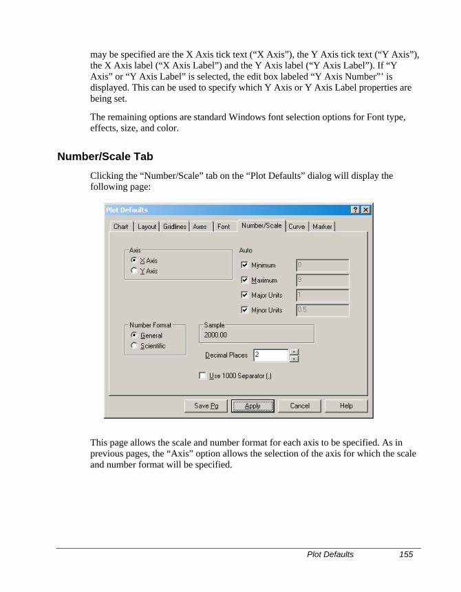
Plot Defaults 155
may be specified are the X Axis tick text (“X Axis”), the Y Axis tick text (“Y Axis”),the X Axis label (“X Axis Label”) and the Y Axis label (“Y Axis Label”). If “YAxis” or “Y Axis Label” is selected, the edit box labeled “Y Axis Number”’ isdisplayed. This can be used to specify which Y Axis or Y Axis Label properties arebeing set.
The remaining options are standard Windows font selection options for Font type,effects, size, and color.
Number/Scale Tab
Clicking the “Number/Scale” tab on the “Plot Defaults” dialog will display thefollowing page:
This page allows the scale and number format for each axis to be specified. As inprevious pages, the “Axis” option allows the selection of the axis for which the scaleand number format will be specified.
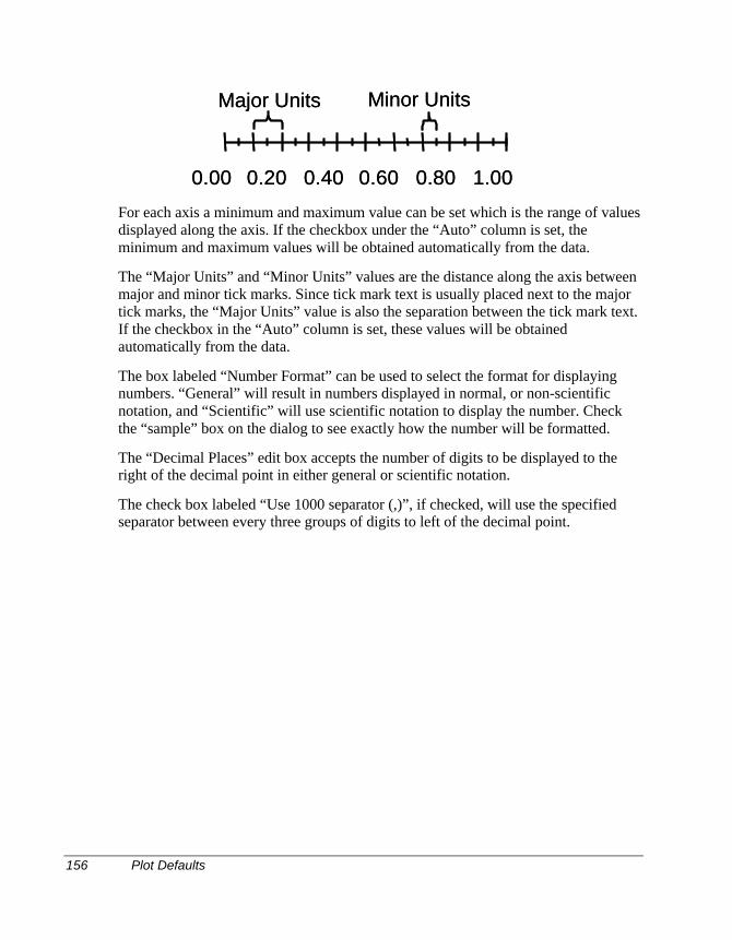
156 Plot Defaults
0.00 0.20 0.40 0.60 0.80 1.00
Major Units Minor Units
0.00 0.20 0.40 0.60 0.80 1.00
Major Units Minor Units
For each axis a minimum and maximum value can be set which is the range of valuesdisplayed along the axis. If the checkbox under the “Auto” column is set, theminimum and maximum values will be obtained automatically from the data.
The “Major Units” and “Minor Units” values are the distance along the axis betweenmajor and minor tick marks. Since tick mark text is usually placed next to the majortick marks, the “Major Units” value is also the separation between the tick mark text.If the checkbox in the “Auto” column is set, these values will be obtainedautomatically from the data.
The box labeled “Number Format” can be used to select the format for displayingnumbers. “General” will result in numbers displayed in normal, or non-scientificnotation, and “Scientific” will use scientific notation to display the number. Checkthe “sample” box on the dialog to see exactly how the number will be formatted.
The “Decimal Places” edit box accepts the number of digits to be displayed to theright of the decimal point in either general or scientific notation.
The check box labeled “Use 1000 separator (,)”, if checked, will use the specifiedseparator between every three groups of digits to left of the decimal point.
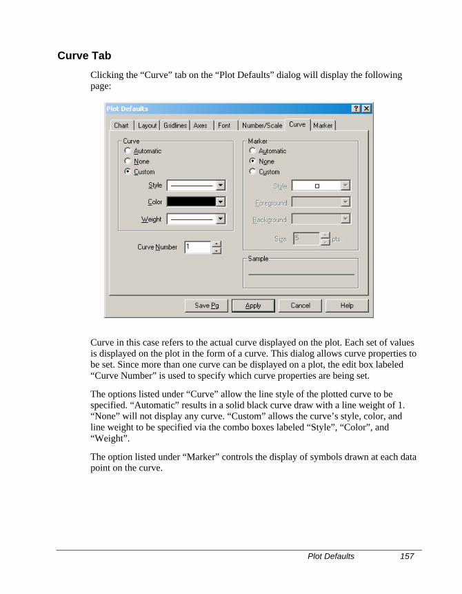
Plot Defaults 157
Curve Tab
Clicking the “Curve” tab on the “Plot Defaults” dialog will display the followingpage:
Curve in this case refers to the actual curve displayed on the plot. Each set of valuesis displayed on the plot in the form of a curve. This dialog allows curve properties tobe set. Since more than one curve can be displayed on a plot, the edit box labeled“Curve Number” is used to specify which curve properties are being set.
The options listed under “Curve” allow the line style of the plotted curve to bespecified. “Automatic” results in a solid black curve draw with a line weight of 1.“None” will not display any curve. “Custom” allows the curve’s style, color, andline weight to be specified via the combo boxes labeled “Style”, “Color”, and“Weight”.
The option listed under “Marker” controls the display of symbols drawn at each datapoint on the curve.
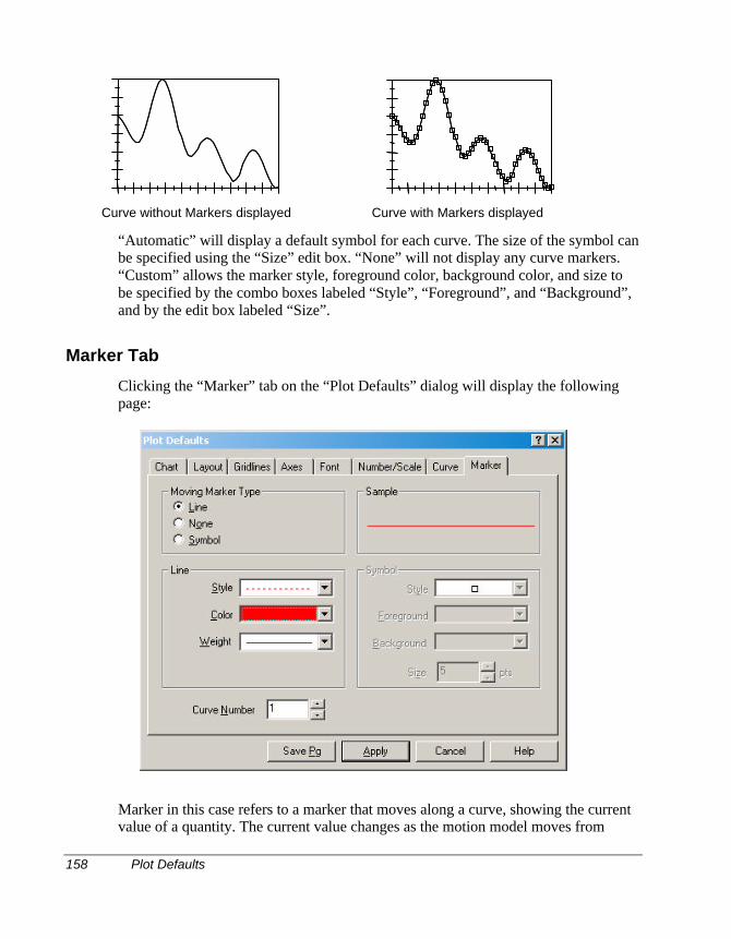
158 Plot Defaults
Curve without Markers displayed Curve with Markers displayed
“Automatic” will display a default symbol for each curve. The size of the symbol canbe specified using the “Size” edit box. “None” will not display any curve markers.“Custom” allows the marker style, foreground color, background color, and size tobe specified by the combo boxes labeled “Style”, “Foreground”, and “Background”,and by the edit box labeled “Size”.
Marker Tab
Clicking the “Marker” tab on the “Plot Defaults” dialog will display the followingpage:
Marker in this case refers to a marker that moves along a curve, showing the currentvalue of a quantity. The current value changes as the motion model moves from
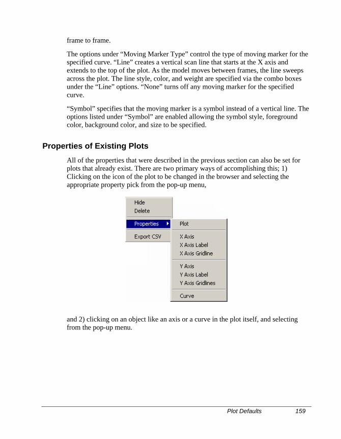
Plot Defaults 159
frame to frame.
The options under “Moving Marker Type” control the type of moving marker for thespecified curve. “Line” creates a vertical scan line that starts at the X axis andextends to the top of the plot. As the model moves between frames, the line sweepsacross the plot. The line style, color, and weight are specified via the combo boxesunder the “Line” options. “None” turns off any moving marker for the specifiedcurve.
“Symbol” specifies that the moving marker is a symbol instead of a vertical line. Theoptions listed under “Symbol” are enabled allowing the symbol style, foregroundcolor, background color, and size to be specified.
Properties of Existing Plots
All of the properties that were described in the previous section can also be set forplots that already exist. There are two primary ways of accomplishing this; 1)Clicking on the icon of the plot to be changed in the browser and selecting theappropriate property pick from the pop-up menu,
and 2) clicking on an object like an axis or a curve in the plot itself, and selectingfrom the pop-up menu.
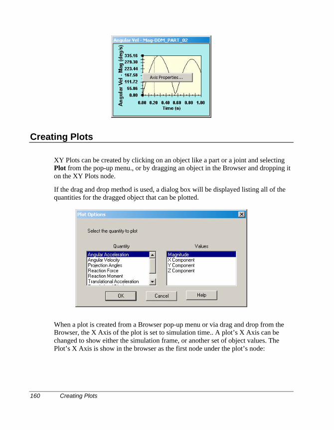
160 Creating Plots
Creating Plots
XY Plots can be created by clicking on an object like a part or a joint and selectingPlot from the pop-up menu., or by dragging an object in the Browser and dropping iton the XY Plots node.
If the drag and drop method is used, a dialog box will be displayed listing all of thequantities for the dragged object that can be plotted.
When a plot is created from a Browser pop-up menu or via drag and drop from theBrowser, the X Axis of the plot is set to simulation time.. A plot’s X Axis can bechanged to show either the simulation frame, or another set of object values. ThePlot’s X Axis is show in the browser as the first node under the plot’s node:
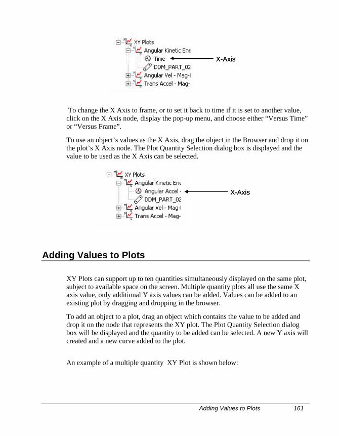
Adding Values to Plots 161
X-AxisX-Axis
To change the X Axis to frame, or to set it back to time if it is set to another value,click on the X Axis node, display the pop-up menu, and choose either “Versus Time”or “Versus Frame”.
To use an object’s values as the X Axis, drag the object in the Browser and drop it onthe plot’s X Axis node. The Plot Quantity Selection dialog box is displayed and thevalue to be used as the X Axis can be selected.
X-AxisX-Axis
Adding Values to Plots
XY Plots can support up to ten quantities simultaneously displayed on the same plot,subject to available space on the screen. Multiple quantity plots all use the same Xaxis value, only additional Y axis values can be added. Values can be added to anexisting plot by dragging and dropping in the browser.
To add an object to a plot, drag an object which contains the value to be added anddrop it on the node that represents the XY plot. The Plot Quantity Selection dialogbox will be displayed and the quantity to be added can be selected. A new Y axis willcreated and a new curve added to the plot.
An example of a multiple quantity XY Plot is shown below:
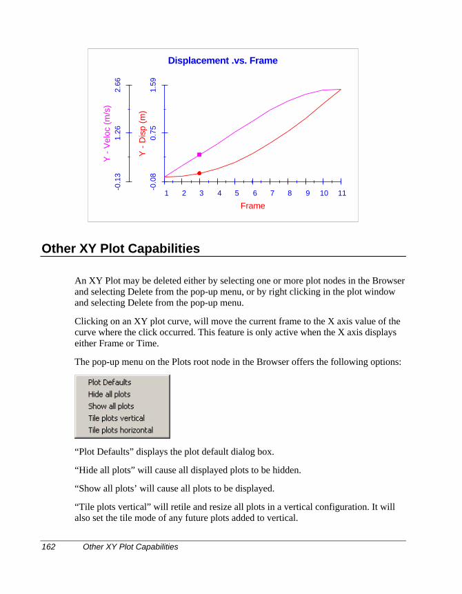
162 Other XY Plot Capabilities
1 2 3 4 5 6 7 8 9 10 11
Frame
-0.0
80.
751.
59Y
- D
isp
(m)
-0.1
31.
262.
66Y
- V
eloc
(m
/s)
Displacement .vs. Frame
Other XY Plot Capabilities
An XY Plot may be deleted either by selecting one or more plot nodes in the Browserand selecting Delete from the pop-up menu, or by right clicking in the plot windowand selecting Delete from the pop-up menu.
Clicking on an XY plot curve, will move the current frame to the X axis value of thecurve where the click occurred. This feature is only active when the X axis displayseither Frame or Time.
The pop-up menu on the Plots root node in the Browser offers the following options:
“Plot Defaults” displays the plot default dialog box.
“Hide all plots” will cause all displayed plots to be hidden.
“Show all plots’ will cause all plots to be displayed.
“Tile plots vertical” will retile and resize all plots in a vertical configuration. It willalso set the tile mode of any future plots added to vertical.
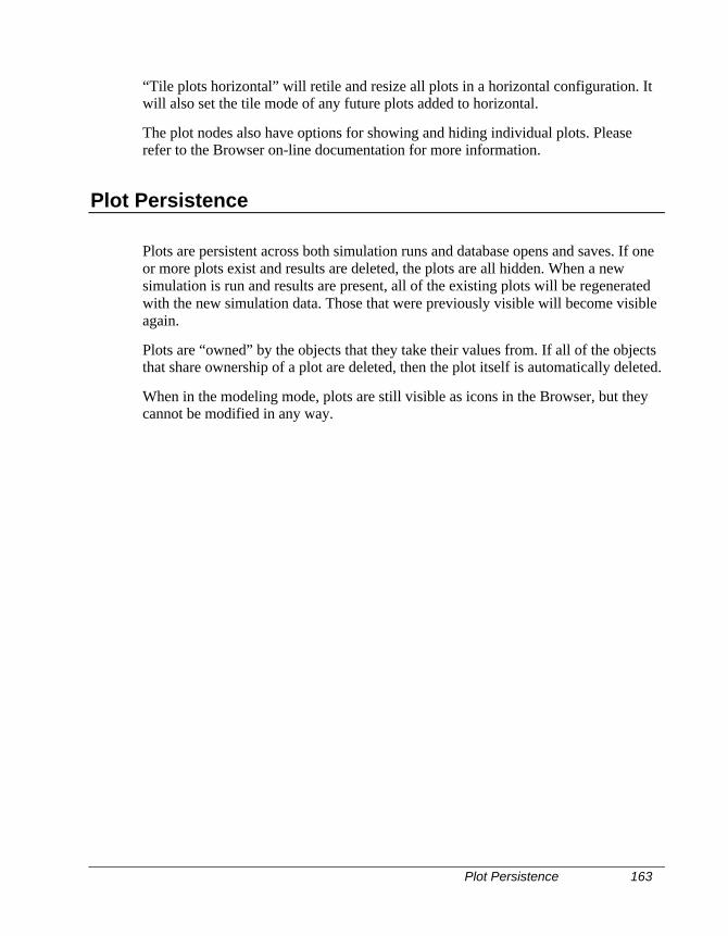
Plot Persistence 163
“Tile plots horizontal” will retile and resize all plots in a horizontal configuration. Itwill also set the tile mode of any future plots added to horizontal.
The plot nodes also have options for showing and hiding individual plots. Pleaserefer to the Browser on-line documentation for more information.
Plot Persistence
Plots are persistent across both simulation runs and database opens and saves. If oneor more plots exist and results are deleted, the plots are all hidden. When a newsimulation is run and results are present, all of the existing plots will be regeneratedwith the new simulation data. Those that were previously visible will become visibleagain.
Plots are “owned” by the objects that they take their values from. If all of the objectsthat share ownership of a plot are deleted, then the plot itself is automatically deleted.
When in the modeling mode, plots are still visible as icons in the Browser, but theycannot be modified in any way.

IntelliMotion Builder Units Page 165
The IntelliMotion Builder is a combination of a tabbed dialog box and a wizard thatleads you step-by-step through the process of changing an Assembly Model into aMotion Model, and performing the Motion simulation.
Any Assembly component that is included in the motion simulation willautomatically be converted in a motion part complete with mass properties. Anyassembly constraints between components included in the motion simulation willautomatically be converted into a motion joint. For assembly models that arecompletely constrained, all that remains to be done after the IntelliMotion Builderhas finished its work is to add motion specified entities like motion generators andsprings. The IntelliMotion Builder is the quickest and most efficient way to performmotion simulation on a Solid Edge Assembly model.
The IntelliMotion Builder is started from the Browser by clicking the Motion Modelnode and choosing IntelliMotion Builder from the pop-up menu or by selecting
IntelliMotion Builder button from the Motion Toolbar.
In the lower left corner of each page in the IntelliMotion Builder are two buttonslabeled <BACK and NEXT>. These buttons can be used to move sequentiallyforward and backwards through the Motion process. The IntelliMotion Builder willnot allow you to proceed to the next step until all of the information required for thecurrent step has been specified.
IntelliMotion Builder Units Page
The first step in the IntelliMotion Builder process is to specify the units that will beused for the Motion Simulation. The information specified on this page is the samethat can be specified using the MOTION OPTIONS command. Units can be
7 IntelliMotion Builder
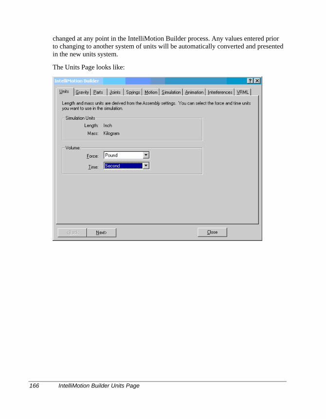
166 IntelliMotion Builder Units Page
changed at any point in the IntelliMotion Builder process. Any values entered priorto changing to another system of units will be automatically converted and presentedin the new units system.
The Units Page looks like:
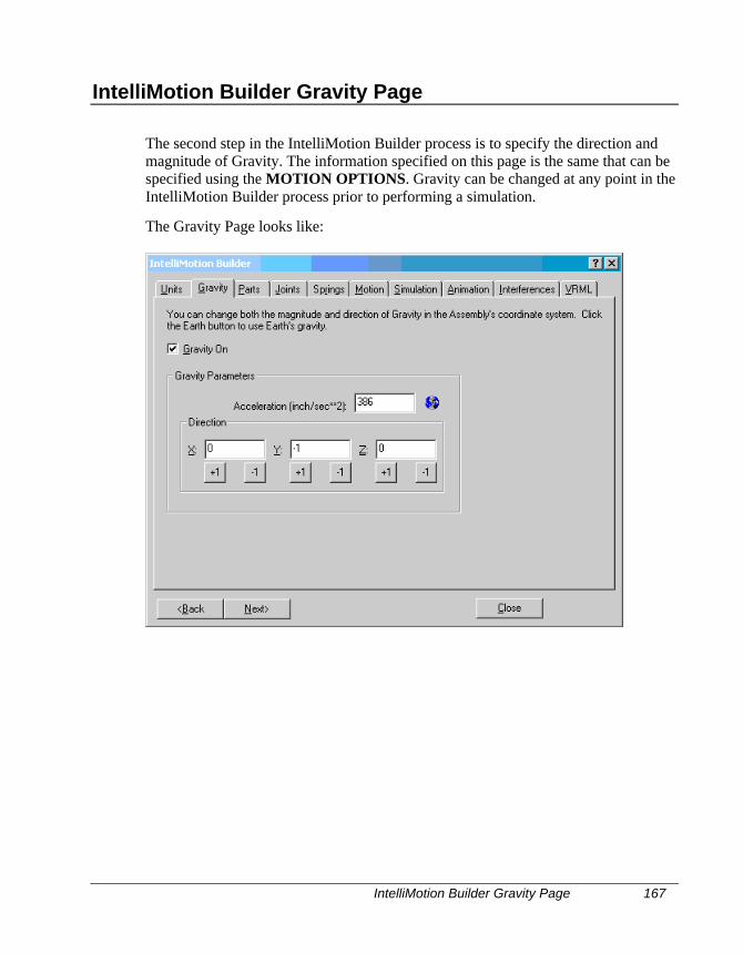
IntelliMotion Builder Gravity Page 167
IntelliMotion Builder Gravity Page
The second step in the IntelliMotion Builder process is to specify the direction andmagnitude of Gravity. The information specified on this page is the same that can bespecified using the MOTION OPTIONS. Gravity can be changed at any point in theIntelliMotion Builder process prior to performing a simulation.
The Gravity Page looks like:
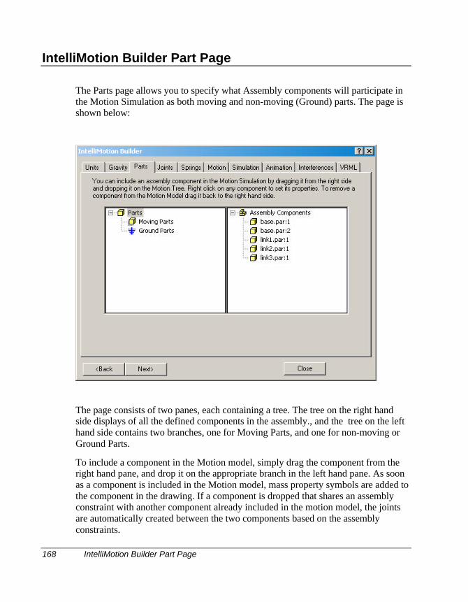
168 IntelliMotion Builder Part Page
IntelliMotion Builder Part Page
The Parts page allows you to specify what Assembly components will participate inthe Motion Simulation as both moving and non-moving (Ground) parts. The page isshown below:
The page consists of two panes, each containing a tree. The tree on the right handside displays of all the defined components in the assembly., and the tree on the lefthand side contains two branches, one for Moving Parts, and one for non-moving orGround Parts.
To include a component in the Motion model, simply drag the component from theright hand pane, and drop it on the appropriate branch in the left hand pane. As soonas a component is included in the Motion model, mass property symbols are added tothe component in the drawing. If a component is dropped that shares an assemblyconstraint with another component already included in the motion model, the jointsare automatically created between the two components based on the assemblyconstraints.
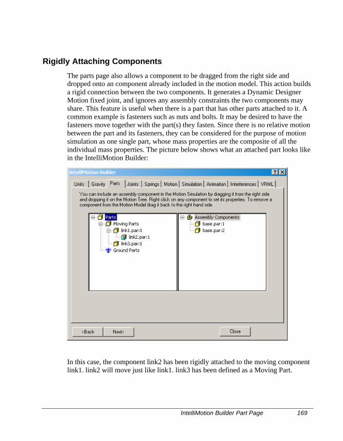
IntelliMotion Builder Part Page 169
Rigidly Attaching Components
The parts page also allows a component to be dragged from the right side anddropped onto an component already included in the motion model. This action buildsa rigid connection between the two components. It generates a Dynamic DesignerMotion fixed joint, and ignores any assembly constraints the two components mayshare. This feature is useful when there is a part that has other parts attached to it. Acommon example is fasteners such as nuts and bolts. It may be desired to have thefasteners move together with the part(s) they fasten. Since there is no relative motionbetween the part and its fasteners, they can be considered for the purpose of motionsimulation as one single part, whose mass properties are the composite of all theindividual mass properties. The picture below shows what an attached part looks likein the IntelliMotion Builder:
In this case, the component link2 has been rigidly attached to the moving componentlink1. link2 will move just like link1. link3 has been defined as a Moving Part.
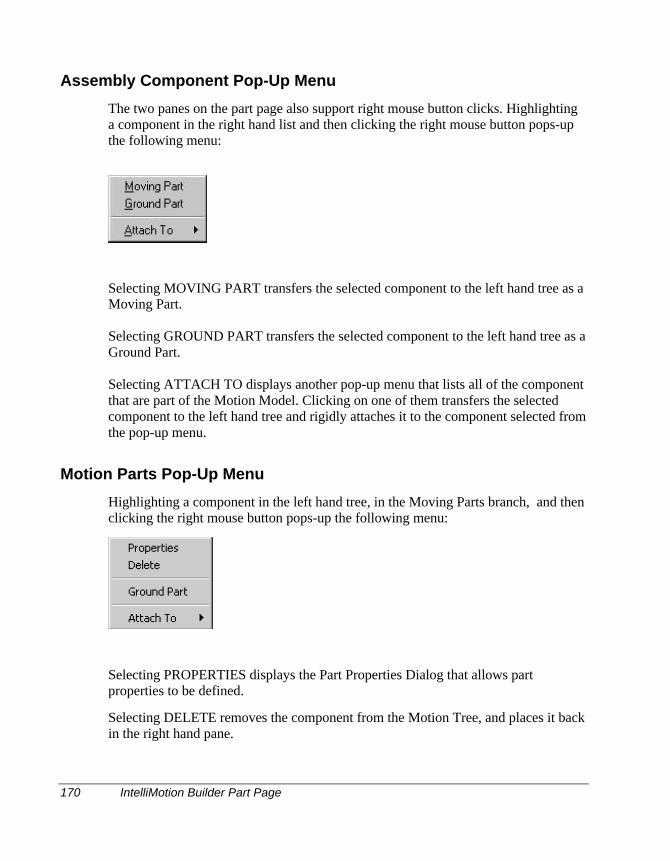
170 IntelliMotion Builder Part Page
Assembly Component Pop-Up Menu
The two panes on the part page also support right mouse button clicks. Highlightinga component in the right hand list and then clicking the right mouse button pops-upthe following menu:
Selecting MOVING PART transfers the selected component to the left hand tree as aMoving Part.
Selecting GROUND PART transfers the selected component to the left hand tree as aGround Part.
Selecting ATTACH TO displays another pop-up menu that lists all of the componentthat are part of the Motion Model. Clicking on one of them transfers the selectedcomponent to the left hand tree and rigidly attaches it to the component selected fromthe pop-up menu.
Motion Parts Pop-Up Menu
Highlighting a component in the left hand tree, in the Moving Parts branch, and thenclicking the right mouse button pops-up the following menu:
Selecting PROPERTIES displays the Part Properties Dialog that allows partproperties to be defined.
Selecting DELETE removes the component from the Motion Tree, and places it backin the right hand pane.
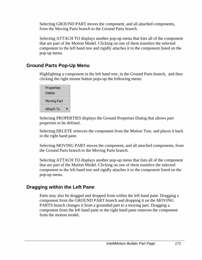
IntelliMotion Builder Part Page 171
Selecting GROUND PART moves the component, and all attached components,from the Moving Parts branch to the Ground Parts branch.
Selecting ATTACH TO displays another pop-up menu that lists all of the componentthat are part of the Motion Model. Clicking on one of them transfers the selectedcomponent to the left hand tree and rigidly attaches it to the component listed on thepop-up menu.
Ground Parts Pop-Up Menu
Highlighting a component in the left hand tree, in the Ground Parts branch, and thenclicking the right mouse button pops-up the following menu:
Selecting PROPERTIES displays the Ground Properties Dialog that allows partproperties to be defined.
Selecting DELETE removes the component from the Motion Tree, and places it backin the right hand pane.
Selecting MOVING PART moves the component, and all attached components, fromthe Ground Parts branch to the Moving Parts branch.
Selecting ATTACH TO displays another pop-up menu that lists all of the componentthat are part of the Motion Model. Clicking on one of them transfers the selectedcomponent to the left hand tree and rigidly attaches it to the component listed on thepop-up menu.
Dragging within the Left Pane
Parts may also be dragged and dropped from within the left hand pane. Dragging acomponent from the GROUND PART branch and dropping it on the MOVINGPARTS branch changes it from a grounded part to a moving part. Dragging acomponent from the left hand pane to the right hand pane removes the componentfrom the motion model.
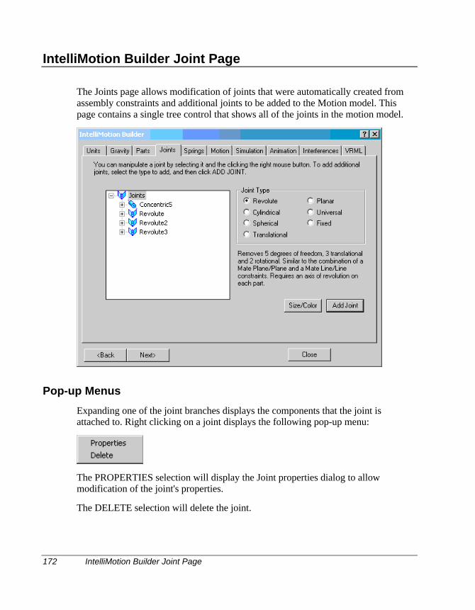
172 IntelliMotion Builder Joint Page
IntelliMotion Builder Joint Page
The Joints page allows modification of joints that were automatically created fromassembly constraints and additional joints to be added to the Motion model. Thispage contains a single tree control that shows all of the joints in the motion model.
Pop-up Menus
Expanding one of the joint branches displays the components that the joint isattached to. Right clicking on a joint displays the following pop-up menu:
The PROPERTIES selection will display the Joint properties dialog to allowmodification of the joint's properties.
The DELETE selection will delete the joint.
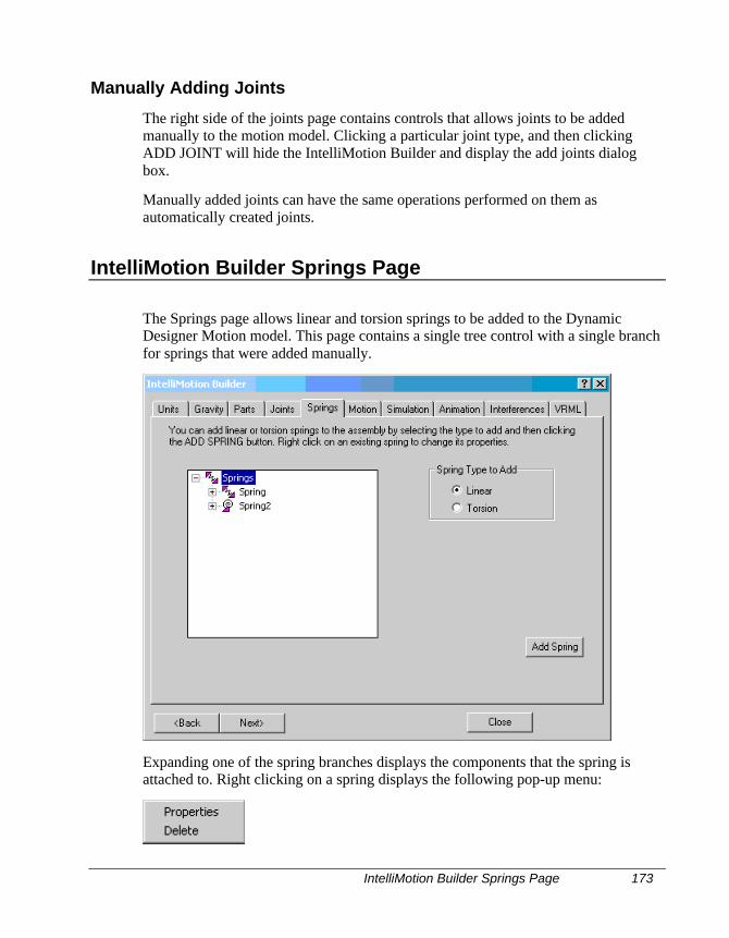
IntelliMotion Builder Springs Page 173
Manually Adding Joints
The right side of the joints page contains controls that allows joints to be addedmanually to the motion model. Clicking a particular joint type, and then clickingADD JOINT will hide the IntelliMotion Builder and display the add joints dialogbox.
Manually added joints can have the same operations performed on them asautomatically created joints.
IntelliMotion Builder Springs Page
The Springs page allows linear and torsion springs to be added to the DynamicDesigner Motion model. This page contains a single tree control with a single branchfor springs that were added manually.
Expanding one of the spring branches displays the components that the spring isattached to. Right clicking on a spring displays the following pop-up menu:
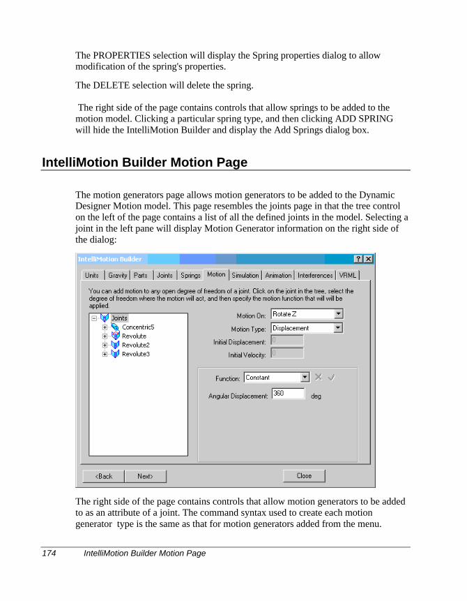
174 IntelliMotion Builder Motion Page
The PROPERTIES selection will display the Spring properties dialog to allowmodification of the spring's properties.
The DELETE selection will delete the spring.
The right side of the page contains controls that allow springs to be added to themotion model. Clicking a particular spring type, and then clicking ADD SPRINGwill hide the IntelliMotion Builder and display the Add Springs dialog box.
IntelliMotion Builder Motion Page
The motion generators page allows motion generators to be added to the DynamicDesigner Motion model. This page resembles the joints page in that the tree controlon the left of the page contains a list of all the defined joints in the model. Selecting ajoint in the left pane will display Motion Generator information on the right side ofthe dialog:
The right side of the page contains controls that allow motion generators to be addedto as an attribute of a joint. The command syntax used to create each motiongenerator type is the same as that for motion generators added from the menu.
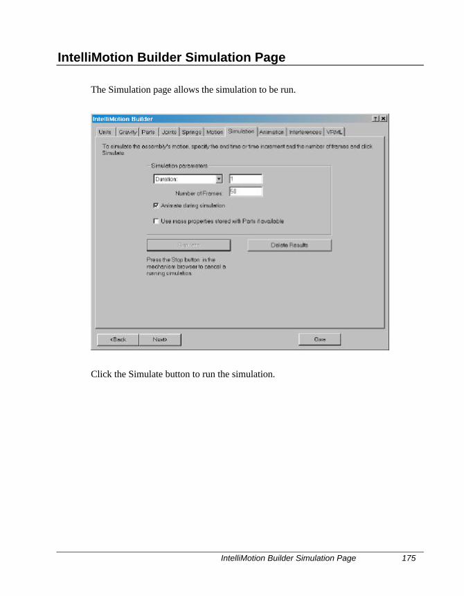
IntelliMotion Builder Simulation Page 175
IntelliMotion Builder Simulation Page
The Simulation page allows the simulation to be run.
Click the Simulate button to run the simulation.
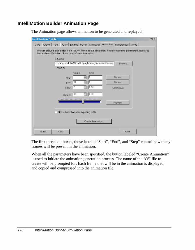
176 IntelliMotion Builder Simulation Page
IntelliMotion Builder Animation Page
The Animation page allows animation to be generated and replayed:
The first three edit boxes, those labeled “Start”, “End”, and “Step” control how manyframes will be present in the animation.
When all the parameters have been specified, the button labeled “Create Animation”is used to initiate the animation generation process. The name of the AVI file tocreate will be prompted for. Each frame that will be in the animation is displayed,and copied and compressed into the animation file.
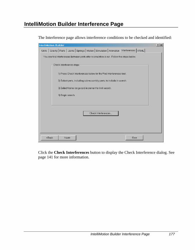
IntelliMotion Builder Interference Page 177
IntelliMotion Builder Interference Page
The Interference page allows interference conditions to be checked and identified:
Click the Check Interferences button to display the Check Interference dialog. Seepage 141 for more information.
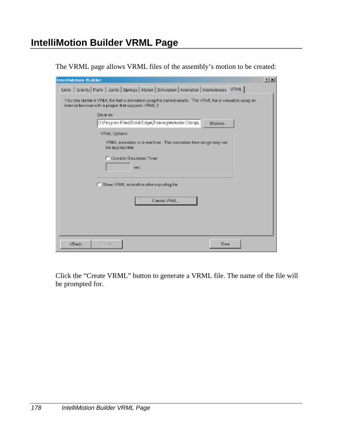
178 IntelliMotion Builder VRML Page
IntelliMotion Builder VRML Page
The VRML page allows VRML files of the assembly’s motion to be created:
Click the “Create VRML” button to generate a VRML file. The name of the file willbe prompted for.
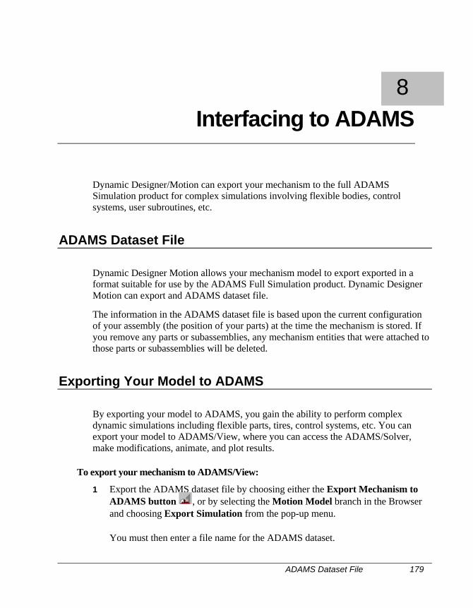
ADAMS Dataset File 179
Dynamic Designer/Motion can export your mechanism to the full ADAMSSimulation product for complex simulations involving flexible bodies, controlsystems, user subroutines, etc.
ADAMS Dataset File
Dynamic Designer Motion allows your mechanism model to export exported in aformat suitable for use by the ADAMS Full Simulation product. Dynamic DesignerMotion can export and ADAMS dataset file.
The information in the ADAMS dataset file is based upon the current configurationof your assembly (the position of your parts) at the time the mechanism is stored. Ifyou remove any parts or subassemblies, any mechanism entities that were attached tothose parts or subassemblies will be deleted.
Exporting Your Model to ADAMS
By exporting your model to ADAMS, you gain the ability to perform complexdynamic simulations including flexible parts, tires, control systems, etc. You canexport your model to ADAMS/View, where you can access the ADAMS/Solver,make modifications, animate, and plot results.
To export your mechanism to ADAMS/View:
1 Export the ADAMS dataset file by choosing either the Export Mechanism toADAMS button , or by selecting the Motion Model branch in the Browserand choosing Export Simulation from the pop-up menu.
You must then enter a file name for the ADAMS dataset.
8 Interfacing to ADAMS
180 Exporting Your Model to ADAMS
2 Save an IGES or STL file for each component.
Open each individual component in your assembly and click File, Save As. Setthe Save as Type field to either IGES files or STL files.
3 Start ADAMS/View and import the ADAMS dataset file.
4 Import each IGES or STL file into ADAMS/View, being sure to attach thegeometry to the correct ADAMS part.
Note: You may need to move the geometry into the correct location.
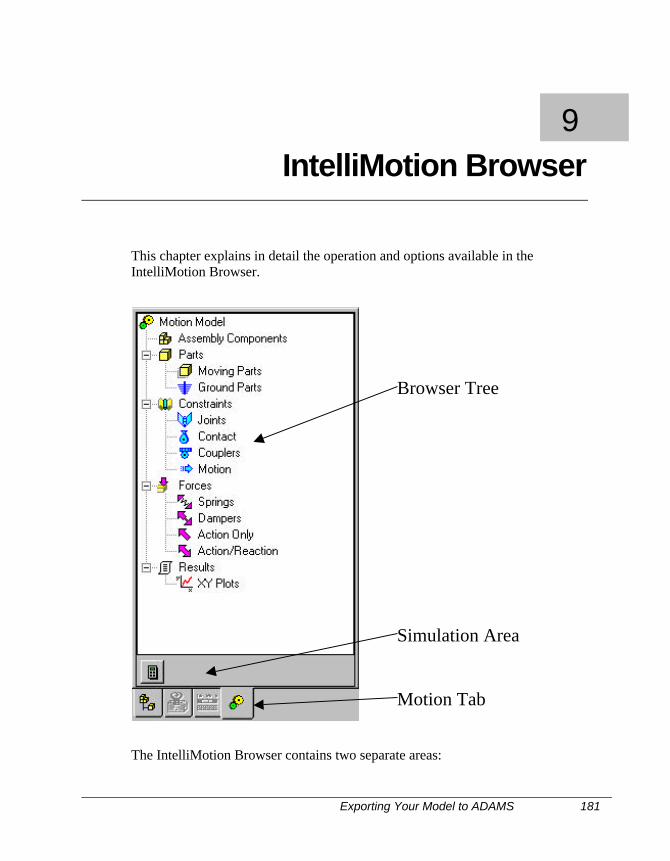
Exporting Your Model to ADAMS 181
This chapter explains in detail the operation and options available in theIntelliMotion Browser.
Browser Tree
Simulation Area
Motion Tab
The IntelliMotion Browser contains two separate areas:
9 IntelliMotion Browser
182 Activating the Browser
1. The Browser Tree is the hierarchical view of the motion model. All drag anddrop operations, and right mouse button activated pop-up menus occur in thisarea.
2. The Simulation Area contains controls that, depending on the mode of themotion model, either starts the simulation or remove simulation results.
Activating the Browser
The IntelliMotion Browser is activated by clicking on the tab in the Solid EdgeEdge Bar.
Note: You must be in the Motion Environment for this.
Detailed Browser Documentation
Due to the extensive amount of information on the Browser and it’s operation, thissection of the documentation is only available in the on-line help. Please see the on-line help topic IntelliMotion Browser for more information.
Function Expression Basics 183
This appendix explains ADAMS function expressions and describes of all of theADAMS functions supported in Dynamic Designer. You can enter these functions inthe expression fields on the motion or force Property panels. You can use thesefunction expressions to define a wide variety of non-standard phenomena in yourmodel. See Creating Motions or Creating Forces for detailed information on how tocreate the function expressions to define a force or a motion.
Function Expression Basics
A function expression is a single C-like or FORTRAN-like expression that evaluatesa single value. This value may be a function of system variables such asdisplacements between markers, velocities, accelerations, and current simulationtime.
Syntax and Notation
A function expression may be composed of any valid combination of simpleconstants, operators, parameters, and available standard ADAMS/Solver functions.
Simple Constants
Function expressions may include integers and real numbers only. Complex numbersare not supported at this time. Any legal number is accepted by the functionexpression. The definition of a legal integer and a legal real number is quite machinedependent, and may therefore change from system to system. Typically inADAMS/Solver, an integer is limited to having an absolute value less than 231 - 1. Areal number in ADAMS/Solver is typically limited to having an absolute value lessthan 1026.
10 ADAMS Functions
184 Function Expression Basics
Operators
ADAMS/Solver allows the standard FORTRAN-77 set of operators. The operatorsand their sequence of evaluation are shown in the table below.
Symbol Operation Precedence** Exponentiation 1/ Division 2* Multiplication 3
A function expression can contain any number of blank spaces. They are often usedto improve the readability of the function expression. The following restrictions existon the usage of blanks:
q You cannot put a blank space in the middle of a number.
q ADAMS/Solver does not accept a blank space between a function and its leftbracket.
Limitations
ADAMS/Solver imposes some limitations in the definition of functions.
Nesting of Functions
Functions, sub-expressions or operations may be nested only ten levels deep. Forexample: FUNCTION = f1 (f2 (f3 (f4))), where f1, f2, f3, f4 are function sub-expressions, is a syntactically legal function definition. However, FUNCTION = f1(f2 (... (f11 ) ...) is not a legal definition, since sub-expressions have been nestedeleven levels deep.
Limitations on Number of Symbols in a Function Expression
A single function expression must not use more than one thousand symbols. Thisincludes operators, brackets, functions, number, etc.
Limitations on Number of Elements to Which a Function Can Refer
A function is limited to being dependent on a maximum of 25 standardADAMS/Solver elements of each type. Therefore, each expression may be a functionof a maximum of 25 PARTS, 25 FORCES, etc.
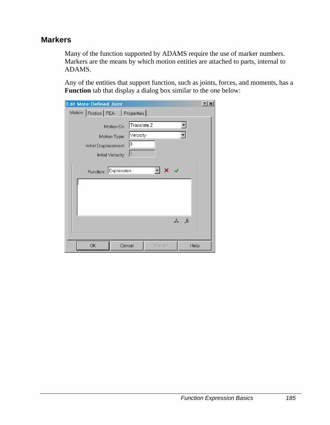
Function Expression Basics 185
Markers
Many of the function supported by ADAMS require the use of marker numbers.Markers are the means by which motion entities are attached to parts, internal toADAMS.
Any of the entities that support function, such as joints, forces, and moments, has aFunction tab that display a dialog box similar to the one below:
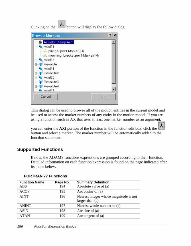
186 Function Expression Basics
Clicking on the button will display the follow dialog:
This dialog can be used to browse all of the motion entities in the current model andbe used to access the marker numbers of any entity in the motion model. If you areusing a function such as AX that uses at least one marker number as an argument,
you can enter the AX( portion of the function in the function edit box, click the button and select a marker. The marker number will be automatically added to thefunction statement.
Supported Functions
Below, the ADAMS functions expressions are grouped according to their function.Detailed information on each function expression is found on the page indicated afterits name below.
FORTRAN 77 Functions
Function Name Page No. Summary DefinitionABS 194 Absolute value of (a)ACOS 195 Arc cosine of (a)AINT 196 Nearest integer whose magnitude is not
larger than (a)ANINT 197 Nearest whole number to (a)ASIN 198 Arc sine of (a)ATAN 199 Arc tangent of (a)
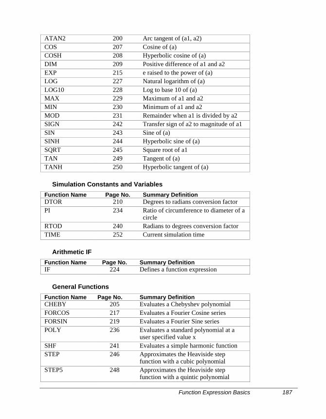
Function Expression Basics 187
ATAN2 200 Arc tangent of (a1, a2)COS 207 Cosine of (a)COSH 208 Hyperbolic cosine of (a)DIM 209 Positive difference of a1 and a2EXP 215 e raised to the power of (a)LOG 227 Natural logarithm of (a)LOG10 228 Log to base 10 of (a)MAX 229 Maximum of a1 and a2MIN 230 Minimum of a1 and a2MOD 231 Remainder when a1 is divided by a2SIGN 242 Transfer sign of a2 to magnitude of a1SIN 243 Sine of (a)SINH 244 Hyperbolic sine of (a)SQRT 245 Square root of a1TAN 249 Tangent of (a)TANH 250 Hyperbolic tangent of (a)
Simulation Constants and Variables
Function Name Page No. Summary DefinitionDTOR 210 Degrees to radians conversion factorPI 234 Ratio of circumference to diameter of a
circleRTOD 240 Radians to degrees conversion factorTIME 252 Current simulation time
Arithmetic IF
Function Name Page No. Summary DefinitionIF 224 Defines a function expression
General Functions
Function Name Page No. Summary DefinitionCHEBY 205 Evaluates a Chebyshev polynomialFORCOS 217 Evaluates a Fourier Cosine seriesFORSIN 219 Evaluates a Fourier Sine seriesPOLY 236 Evaluates a standard polynomial at a
user specified value xSHF 241 Evaluates a simple harmonic functionSTEP 246 Approximates the Heaviside step
function with a cubic polynomialSTEP5 248 Approximates the Heaviside step
function with a quintic polynomial
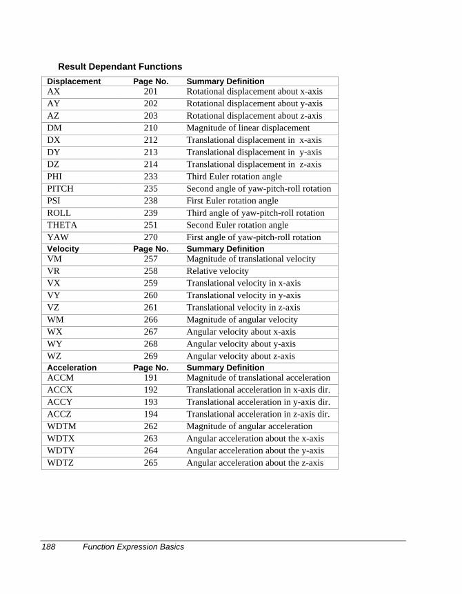
188 Function Expression Basics
Result Dependant Functions
Displacement Page No. Summary DefinitionAX 201 Rotational displacement about x-axisAY 202 Rotational displacement about y-axisAZ 203 Rotational displacement about z-axisDM 210 Magnitude of linear displacementDX 212 Translational displacement in x-axisDY 213 Translational displacement in y-axisDZ 214 Translational displacement in z-axisPHI 233 Third Euler rotation anglePITCH 235 Second angle of yaw-pitch-roll rotationPSI 238 First Euler rotation angleROLL 239 Third angle of yaw-pitch-roll rotationTHETA 251 Second Euler rotation angleYAW 270 First angle of yaw-pitch-roll rotationVelocity Page No. Summary DefinitionVM 257 Magnitude of translational velocityVR 258 Relative velocityVX 259 Translational velocity in x-axisVY 260 Translational velocity in y-axisVZ 261 Translational velocity in z-axisWM 266 Magnitude of angular velocityWX 267 Angular velocity about x-axisWY 268 Angular velocity about y-axisWZ 269 Angular velocity about z-axisAcceleration Page No. Summary DefinitionACCM 191 Magnitude of translational accelerationACCX 192 Translational acceleration in x-axis dir.ACCY 193 Translational acceleration in y-axis dir.ACCZ 194 Translational acceleration in z-axis dir.WDTM 262 Magnitude of angular accelerationWDTX 263 Angular acceleration about the x-axisWDTY 264 Angular acceleration about the y-axisWDTZ 265 Angular acceleration about the z-axis
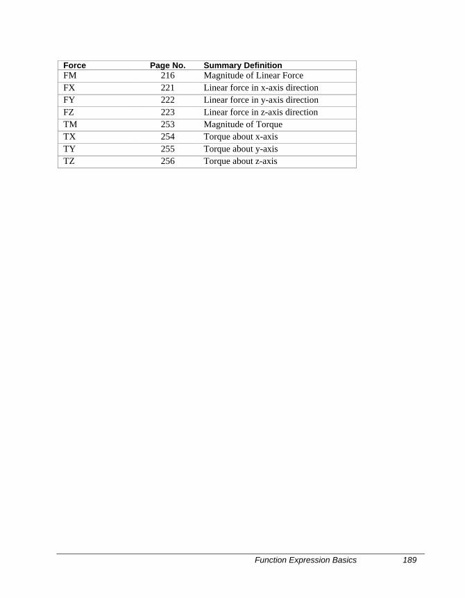
Function Expression Basics 189
Force Page No. Summary DefinitionFM 216 Magnitude of Linear ForceFX 221 Linear force in x-axis directionFY 222 Linear force in y-axis directionFZ 223 Linear force in z-axis directionTM 253 Magnitude of TorqueTX 254 Torque about x-axisTY 255 Torque about y-axisTZ 256 Torque about z-axis
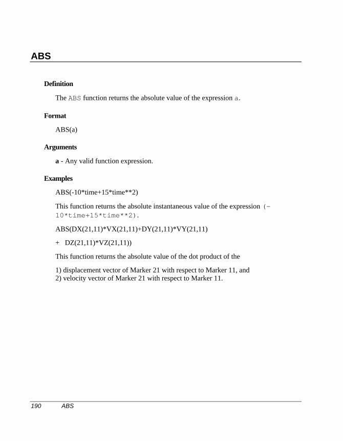
190 ABS
ABS
Definition
The ABS function returns the absolute value of the expression a.
Format
ABS(a)
Arguments
a - Any valid function expression.
Examples
ABS(-10*time+15*time**2)
This function returns the absolute instantaneous value of the expression (-10*time+15*time**2).
ABS(DX(21,11)*VX(21,11)+DY(21,11)*VY(21,11)
+ DZ(21,11)*VZ(21,11))
This function returns the absolute value of the dot product of the
1) displacement vector of Marker 21 with respect to Marker 11, and2) velocity vector of Marker 21 with respect to Marker 11.
ACCM 191
ACCM
Definition
The ACCM function calculates the magnitude of the second time derivative of thedisplacement vector of marker i from marker j. The time derivatives are taken in thereference frame of marker l. Markers j and l default to the global coordinate systemand the global reference frame if they are not specified.
Format
ACCM(i[,j ][,l ])
Arguments
i The marker whose acceleration is being measured.
j The marker with respect to which the acceleration is being measured. Set j =0, while still specifying l, if you want j default to the global coordinatesystem.
l The reference frame in which the second time derivative of the displacementvector is taken. Set l = 0 if you want the time derivatives to be calculated inthe ground reference frame.
Examples
ACCM(21,11)
This statement obtains the magnitude of translational acceleration of Marker 21 withrespect to Marker 11. Since the l marker is not specified, the derivatives are taken inthe inertial reference frame.
ACCM(21,11,32)
This statement obtains the magnitude of the translational acceleration of Marker 21with respect to Marker 11. Vector time derivatives taken in reference to Marker 32.
192 ACCX
ACCX
Definition
The ACCX function returns the x-component of the difference between theacceleration vector of marker i and the acceleration vector of marker j as computed inthe coordinate system of marker k. All vector time derivatives are taken in thereference frame of marker l. Marker j defaults to the global coordinate system if it isnot specified. Similarly, markers k and l default to the global coordinate system andthe global reference frame if they are not specified.
Format
ACCX(i[,j][,k][,l ])
Arguments
i The marker whose acceleration is being measured.
j The marker with respect to which the acceleration is being measured. Set j= 0, while still specifying l, if you want j to default to the global coordinatesystem.
k The marker in whose coordinate system the acceleration vector is beingexpressed. Set k = 0 if you want the results to be calculated along the x-axisof the global coordinate system.
l The reference frame in which the second time derivative of the displacementvector is taken. Set l = 0 if you want the time derivatives to be taken in theground reference frame.
Examples
ACCX(21,0,31)
This statement obtains the x-component of the acceleration vector of Marker 21 withrespect to the global origin. The vector is expressed in the coordinate system ofMarker 31. All time derivatives are taken in the inertial reference frame since the lmarker is not specified.
ACCY 193
ACCY
Definition
The ACCY function returns the y-component of the difference between theacceleration vector of marker i and the acceleration vector of marker j as computed inthe coordinate system of marker k. All vector time derivatives are taken in thereference frame of marker l. Marker j defaults to the global coordinate system if it isnot specified. Similarly, markers k and l default to the global coordinate system andthe global reference frame if they are not specified.
Format
ACCY(i[,j ][,k][,l ])
Arguments
i The marker whose acceleration is being measured.
j The marker with respect to which the acceleration is being measured. Set j =0, while still specifying l, if you want j to default to the global coordinatesystem.
k The marker in whose coordinate system the acceleration vector is beingexpressed. Set k = 0 if you want the results to be calculated along the y-axisof the global coordinate system.
l The reference frame in which the second time derivative of the displacementvector is taken. Set l = 0 if you want the time derivatives to be taken in theground reference frame.
Examples
ACCY(21,11)
This statement obtains y-component of the acceleration of Marker 21 with respect toMarker 11. The coordinate system for calculating the component, and for referencingthe frame that takes time derivatives, defaults to ground.
194 ACCZ
ACCZ
Definition
The ACCZ function returns the z-component of the difference between theacceleration vector of marker i and the acceleration vector of marker j as computed inthe coordinate system of marker k. All vector time derivatives are taken in thereference frame of marker l. Marker j defaults to the global coordinate system if it isnot specified. Similarly, markers k and l default to the global coordinate system andthe global reference frame if they are not specified.
Format
ACCZ(i [,j][,k][,l ])
Arguments
i The marker whose acceleration is being measured.
j The marker with respect to which the acceleration is being measured. Set j =0, while still specifying l, if you want j default to the global coordinatesystem.
k The marker in whose coordinate system the acceleration vector is beingexpressed. Set k = 0 if you want the results to be calculated along the z-axisof the global coordinate system.
l The reference frame in which the first time derivative of the displacementvector is taken. Set l = 0 if you want the time derivatives to be taken in theground reference frame.
Example
ACCZ(21,0,31)
This statement obtains the z-component of the acceleration vector of Marker 21 withrespect to the global origin. The vector is expressed in the coordinate system ofMarker 31. All time derivatives are taken in the inertial reference frame since the lmarker is not specified.
ACOS 195
ACOS
Definition
The ACOS function calculates the arc cosine of an expression a. Expression a mustevaluate to a value whose absolute value is less than or equal to 1. The value returnedby ACOS lies in the range [0,p] (i.e., 0 ACOS(a) p).
Format
ACOS(a)
Arguments
a - Any valid function expression.
Examples
ACOS((DX(21,11)*DX(31,41)+DY(21,11)*DY(31,41)
+ DZ(21,11)*DZ(31,41))/(DM(21,11)*DM(31,41))
This function calculates the angle between the line from Markers 11 to 21 and theline from Markers 41 to 31. The result is in radians.
196 AINT
AINT
Definition
The AINT function returns the nearest integer whose magnitude is not larger than theinteger value of the expression a.
AINT(a)= 0 if ABS(a)< 1
AINT(a)=int(a) if ABS(a) 1
The value of the mathematical function int of a variable x is equal to x if x is aninteger. If x is not an integer, then int(x) is equal to the nearest integer to x whosemagnitude is not greater than the magnitude of x. Thus int(-7.0) = -7, int(-4.8) = -4, and int(4.8) = 4.
Format
AINT(a)
Arguments
a - Any valid function expression.
Cautions
Note that AINT is not a differentiable function. Be careful when using this functionin an expression that defines a force or motion input to the system.
Examples
AINT(-6.5)= 0
AINT(4.6)= 4
ANINT 197
ANINT
Definition
The ANINT function calculates the nearest integer whose magnitude is not largerthan the real value of the expression a.
ANINT(a) = int(a + .5) if a 0
ANINT(a) = int(a - .5) if a < 0
The value of the mathematical function int of a variable x is equal to x if x is aninteger. If x is not an integer, then int(x) is equal to the nearest integer to x whosemagnitude is not greater than the magnitude of x. Thus int(-7.0) = -7, int(-4.8) = -4, and int(4.8) = 4.
Format
ANINT(a)
Arguments
a - Any valid function expression.
Examples
ANINT(-4.6)= -5
ANINT(4.6)= 5
198 ASIN
ASIN
Definition
The ASIN function computes the arc sine of an expression a. ASIN is defined onlywhen the absolute value of a is less than or equal to 1. The range of ASIN is [-p/2, p/2] (i.e., -p/2 ASIN(a) p/2).
Format
ASIN(a)
Arguments
a - Any valid function expression.
Examples
ASIN(DX(21,11)/DM(21,11))
This function calculates the value of the expression DX(21,11)/DM(21,11) andthen applies the ASIN function to the result. The result is in radians.
ATAN 199
ATAN
Definition
The ATAN function returns the arc tangent of an expression a. The range of ATAN is[-p/2, p/2] (i.e., -p/2 < ATAN(a)< p/2).
Format
ATAN(a)
Arguments
a - Any valid function expression.
Examples
SFORCE/1, ROTATIONAL, I=21, J=11
, FUNCTION=-10*ATAN(DY(42,33)/DX(42,33))
This SFORCE statement defines a torque acting between Markers 21 and 11. Thevalue of the torque is the spring constant (10) multiplied by the angle between theline joining Markers 33 and 42 and the global x-axis.
200 ATAN2
ATAN2
Definition
The ATAN2 function expression returns the arc tangent of the expression a1/a2.a1 and a2 themselves may be expressions.
-p < ATAN2(a1,a2) < p
ATAN2(a1,a2) > 0 if a1 > 0
ATAN2(a1,a2) = 0 if a1 = 0, a2 > 0
ATAN2(a1,a2) = p if a1 = 0, a2 < 0
ATAN2(a1,a2) < 0 if a1 < 0
ABS(ATAN2(a1,a2))= p/2 if a2 = 0
ATAN2(a1,a2) undefined if a1 = 0, and a2 = 0
Format
ATAN2(a1,a2)
Arguments
a1 - Any valid function expression.
a2 - Any valid function expression.
Examples
VARIABLE/1,
, FUNCTION=ATAN2(DY(21,31,41), DX(21,31,41))
This VARIABLE statement defines an algebraically-determined, user-defined statevariable in ADAMS/Solver. Its value is specified by the expression containingATAN2.
AX 201
AX
Definition
The AX function returns the rotational displacement of marker i about the x-axis ofmarker j. Marker j defaults to the global coordinate system if it is not specified.This value is computed as follows: assume that rotations about the other two axes (y-, z-axes) of marker j are zero. Then AX is the angle between the two y-axes (or thetwo z-axes). AX is measured in a counter- clockwise sense from the y-axis of the Jmarker to the y-axis of the I marker.
Format
AX(i[,j])
Arguments
i The marker whose rotations are being sought.
j The marker with respect to which the rotations are being measured.
Examples
-20*AX(43,32)
The value of the function is -20 times the angle between the y axes of Markers 43and 32. The angle is measured in a counterclockwise sense from the y-axis of Marker32 to the y-axis of Marker 43.
202 AY
AY
Definition
The AY function returns the rotational displacement of marker i about the y-axis ofmarker j. Marker j defaults to the global coordinate system if it is not specified.This value is computed as follows: assume that rotations about the other two axes (x-, z-axes) of marker j are zero. Then AY is the angle between the two x-axes (or thetwo z-axes). AY is measured in a counter- clockwise sense from the x-axis of the Jmarker to the x-axis of the I marker.
Format
AY(i[,j])
Arguments
i The marker whose rotations are being sought.
j The marker with respect to which the rotations are being measured.
Examples
-4*(AY(46,57)**2)
The value of the function is -4 times the square of the angle between the x axes ofMarkers 46 and 57. The angle is measured in a counterclockwise sense from the x-axis of Marker 57 to the x-axis of Marker 46.
AZ 203
AZ
Definition
The AZ function returns the rotational displacement of marker i about the z-axis ofmarker j. Marker j defaults to the global coordinate system if it is not specified.This value is computed as follows: assume that rotations about the other two axes (x-, y-axes) of marker j are zero. Then AZ is the angle between the two x-axes (or thetwo y-axes). AZ is measured in a counter- clockwise sense from the x-axis of the Jmarker to the x-axis of the I marker.
Format
AZ(i[,j])
Arguments
i The marker whose rotations are being sought.
j The marker with respect to which the rotations are being measured.
Examples
-30*(AZ(21,32)-25D)
204 BISTOP
BISTOP
Definition
The BISTOP function models a gap element.
Format
BISTOP (x, x& , x1, x2, k, e, cmax, d)
Arguments
x A real variable that specifies the distance variable you want to use tocompute the force. For example, if you want to use the x displacement ofMarker 0201 with respect to 0301, then x is DX(0201,0301,0301).
x& A real variable that communicates the time derivative of x to BISTOP. Forexample, if x is DX(0201,0301,301)then x& isVX(0201,0301,0301,0301).
x1 A real variable that specifies the lower bound of x. If x is less than x1ADAMS/Solver calculates a positive value for the force. The value of x1must be less than the value of x2.
x2 A real variable that specifies the upper bound of x. If x is greater than x2ADAMS/Solver calculates a negative value for the force. The value of x2must be greater than the value of x1.
k A non-negative real variable that specifies the stiffness of the boundarysurface interaction.
e A positive real variable that specifies the exponent of the force deformationcharacteristic. For a stiffening spring characteristic, e > 1.0. For a softeningspring characteristic, 0 < e < 1.0.
cmax A non-negative real variable that specifies the maximum dampingcoefficient.
d A positive real variable that specifies the boundary penetration at whichADAMS/Solver applies full damping.
CHEBY 205
Extended Definition
The BISTOP function models a gap element. The gap element consists of a slotwhich defines the domain of motion of a Part I located in the slot. As long as Part I islocated in the slot and has no interference with the ends of the slot, it is free to movewithout forces acting on it. When Part I tries to move beyond the physical definitionof the slot, impact forces representing contact are created by the BISTOP function.The created force tends to move Part I back into the slot.
The BISTOP force has two components: A stiffness component dependent on thepenetration of Part I into the restricting Part J and a damping or viscous componentthat may be used to model energy loss.
To prevent a discontinuity in the damping force at zero penetration, the dampingcoefficient is defined as a cubic step function of the penetration. Thus at zeropenetration, the damping coefficient is always zero. The damping coefficientachieves a maximum, cmax, at a user-defined penetration, d. Even though the pointsof contact between the floating part and the restricting part may change as the systemmoves, ADAMS/Solver always exerts the force between the I and the J markers.
CHEBY
Definition
The CHEBY function evaluates a Chebyshev polynomial at a user specified value x.
Format
CHEBY (x, x0, a0, a1,..., a30)
Arguments
x - A real variable that specifies the independent variable. For example, if theindependent variable in the function is time, x is the system variable TIME.
x0 - A real variable that specifies a shift in the Chebyshev polynomial.
a0,a1,...,a30 - The real variables that define as many as thirty-one coefficients for theChebyshev polynomial.
206 CHEBY
Extended Definition
The CHEBY function evaluates a Chebyshev polynomial at a user specified value x.x0, a0, a1,..., a30 are parameters used to define the constants for theChebyshev polynomial. The Chebyshev polynomial is defined as:
C(x) = å aj Tj (x-x0)
where the functions Tj are recursively defined as:
Tj (x-x0) = 2 * (x-x0) * Tj-1 (x-x0) - Tj-2 (x-x0)
where T0 (x-x0) = 1, and T1 (x-x0) = x-x0.
The index “j” has a range from zero to “n”, where “n” is the number of terms in theseries.
Note that:
T2 (x-x0) = 2 * (x- x0)2 - 1
T3 (x-x0) = 4 * (x- x0)3 - 3 * (x- x0)
Examples
MOTION/1, JOINT=21, TRANSLATION,
,FUNCTION = IF (TIME-2:CHEBY(TIME, 1, 1, 0, -1), 0, 0)
This MOTION statement defines a motion using a quadratic Chebyshev polynomialand the system variable TIME. The arithmetic IF ensures that the function remainszero after 2 time units. When time is less than 2 time units, ADAMS/Solver evaluatesa Chebyshev polynomial to determine the motion. The polynomial defined in theabove example is:
Cheby = 1 + 0 * (time-1) - 1 * [2 (time-1)2 - 1] = 2*time2 - 4*time
COS 207
COS
Definition
The COS function returns the cosine of an expression a.
Format
COS(a)
Arguments
a - Any valid function expression.
Examples
MOTION/2060, JOINT=2060, ROTATION,
, FUNCTION=20D+COS(2*PI*TIME)
This MOTION statement defines a rotational motion acting on JOINT/2060. Therotational degrees of freedom is specified to be the function20D+COS(2*PI*TIME).
208 COSH
COSH
Definition
The COSH function computes the hyperbolic cosine of an expression a.
COSH(a) = (ea + e-a) / 2.0
Format
COSH(a)
Arguments
a - Any valid function expression.
Examples
REQUEST/36,
, F2=COSH(DZ(21,11,11))
This REQUEST statement returns the hyperbolic cosine of the z-component of thedisplacement of Marker 21 with respect to Marker 11 in its second column. Theresult is computed in the coordinate system of Marker 11.
DIM 209
DIM
Definition
The DIM function calculates the positive difference of the instantaneous values oftwo expressions a1 and a2.
DIM(a1,a2) = 0 if a1 a2
DIM(a1,a2) =a1-a2 if a1 > a2
Format
DIM(a1,a2)
Arguments
a1 - Any valid function expression.
a2 - Any valid function expression.
Cautions
q DIM is a discontinuous function and must be used with caution.
210 DM
DM
Definition
The DM function returns the magnitude of the translational displacement vector frommarker j to marker i. Marker j defaults to the global coordinate system if it is notspecified. DM is the distance between markers i and j and by definition is alwaysnon-negative.
Format
DM(i[,j])
Arguments
i The marker whose origin is being measured.
j The marker whose origin is the reference point for the displacementcalculation.
Examples
-30*(DM(21,11)-25)**1.72
DTOR 211
DTOR
Definition
The DTOR function returns the degrees to radians conversion factor (PI/180).
Format
DTOR
Examples
VARIABLE/1, FUNCTION=30*DTOR*TIME
This VARIABLE statement specifies a user-defined, algebraically-determined statevariable whose value is 30 degrees*time. The state variable is stored in radians.
212 DX
DX
Definition
Returns the x-component of the translational displacement vector from marker j tomarker i as expressed in marker k coordinate system. Marker j defaults to theglobal coordinate system if it is not specified. Similarly, marker k defaults to groundif it is not specified.
Format
DX(i[,j][,k])
Arguments
i The marker whose origin is being measured.
j The marker whose origin is the reference point for the displacementcalculation.
k The marker in whose coordinates the x-component of the displacementvector is being calculated. Set k = 0 if you want the results to be calculatedalong the x-axis of the global coordinate system.
Examples
DX(21,11,32)**2
This function is the square of the x-displacement of Marker 21 with respect toMarker 11 as computed in the coordinate system of Marker 32.
DY 213
DY
Definition
The DY function returns the y-component of the translational displacement vectorfrom marker j to marker i as expressed in the marker k coordinate system.Marker j defaults to the global coordinate system if it is not specified. Similarly,marker k defaults to the global coordinate system if it is not specified.
Format
DY(i[,j][,k])
Arguments
i The marker whose origin is being measured.
j The marker whose origin is the reference point for the displacementcalculation. Set j=0 if you want j to default to the global coordinate systemwhile still specifying l.
k The marker in whose coordinates the y-component of the displacementvector is being calculated. Set k = 0 if you want the results to be calculatedalong the x-axis of the global coordinate system.
Examples
DY(21,11,32)**2
This function is the square of the y-displacement of Marker 21 with respect toMarker 11 as computed in the coordinate system of Marker 32.
214 DZ
DZ
Definition
The DZ function returns the z-component of the translational displacement vectorfrom marker j to marker i as expressed in the marker k coordinate system. Markerj defaults to the global coordinate system if it is not specified. Similarly marker kdefaults to the global coordinate system if it is not specified.
Format
DZ(i[,j][,k])
Arguments
i The marker whose origin is being measured.
j The marker whose origin is the reference point for the displacementcalculation. Set j=0 if you want j to default to the global coordinate systemwhile still specifying l.
k The marker in whose coordinates the z-component of the displacementvector is being calculated. Set k = 0 if you want the results to be calculatedalong the x-axis of the global coordinate system.
Examples
DZ(21,11,32)**2
This function is the square of the z-displacement of Marker 21 with respect toMarker 11 as computed in the coordinate system of Marker 32.
EXP 215
EXP
Definition
The EXP function computes the value ea, where a is any expression.
Format
EXP(a)
Arguments
a - Any valid function expression.
Examples
REQUEST/10, F2=EXP(WDTX(21,11,11,31))
In its second column, REQUEST/10 stores the value eWDTX(21,11,11,31).
216 FM
FM
Definition
The FM function returns the magnitude of the net translational force acting at markeri due to all applied forces and constraints acting between markers i and j. Tocalculate the magnitude of the net translational force at marker i due to action-onlyforces acting at i, set j = 0 or do not specify the j marker.
Format
FM(i [ , j ] )
Arguments
i An integer that specifies the identifier of the marker at which the magnitudeof the net force is to be calculated.
j A second integer that specifies a marker identifier. All forces acting betweenthe [i,j] pair are included in the calculation. Set j = 0 or do not specify it if youare interested in action-only forces.
Examples
VARIABLE/1, FUNCTION=FM(23)
A user-defined state variable is specified by this VARI ABLE statement. Its value isthe magnitude of the sum of all action-only forces acting at Marker 23.
VARIABLE/1, FUNCTION=FM(23,11)
A user-defined state variable is specified by this VARI ABLE statement. Its value isthe magnitude of the sum of all the forces at Marker 23 and acting between Markers23 and 11.
FORCOS 217
FORCOS
Definition
The FORCOS function evaluates a Fourier Cosine series at a user specified value x.x0 a0,a1,...,a30 are parameters used to define the constants for the Fourier Cosineseries.
Format
FORCOS (x, x0, w, a0, a1,..., a30)
Arguments
x - A real variable that specifies the independent variable. For example, if theindependent variable in the function is time, x is the system variable TIME.
x0 - A real variable that specifies a shift in the Fourier Cosine series.
w - A real variable that specifies the fundamental frequency of the series.ADAMS/Solver assumes w is in radians per unit of the independent variable unlessyou use a D after the value.
a0,a1,...,a30 - The real variables that define as many as thirty-one coefficients for theFourier Cosine series.
Extended Definition
The Fourier Cosine series is defined:
F(x) = a0 + * Tj (x-x0)
where the functions Tj are defined as:
Tj (x-x0) = cos{j * w * (x-x0)}
The index j has a range from 1 to n, where n is the number of terms in the series.
Examples
MOTION/1, JOINT=21, TRANSLATION,
, FUNCTION=FORCOS(TIME, 0, 360D, 1, 2, 3, 4)
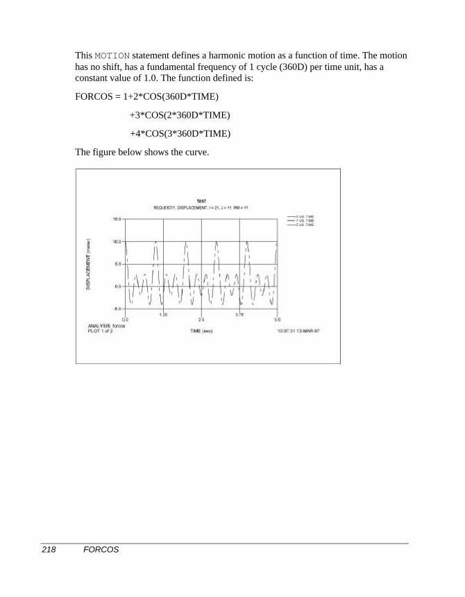
218 FORCOS
This MOTION statement defines a harmonic motion as a function of time. The motionhas no shift, has a fundamental frequency of 1 cycle (360D) per time unit, has aconstant value of 1.0. The function defined is:
FORCOS = 1+2*COS(360D*TIME)
+3*COS(2*360D*TIME)
+4*COS(3*360D*TIME)
The figure below shows the curve.
FORSIN 219
FORSIN
Definition
The FORSIN function evaluates a Fourier Sine series at a user specified value x.x0,a0,a1,...,a30 are parameters used to define the constants for the Fourier Sine series.
Format
FORSIN (x, x0, w, a0, a1,..., a30)
Arguments
x - A real variable that specifies the independent variable. For example, if theindependent variable in the function is time, x is the system variable TIME.
x0 - A real variable that specifies a shift in the Fourier Sine series.
w - A real variable that specifies the fundamental frequency of the series.ADAMS/Solver assumes w is in radians per unit of the independent variable unlessyou use a D after the value.
a0 - A real variable that defines the constant bias term for the function.
a1,...,a30 - The real variables that define as many as thirty-one coefficients for theFourier Sine series.
Extended Definition
The Fourier Sine series is defined:
F(x) = a0 + * Tj (x-x0)
where the functions Tj are defined as:
Tj (x-x0) = sin{j * w * (x-x0)}
The index j has a range from 1 to n, where n is the number of terms in the series
Examples
MOTION/1, JOINT=21, TRANSLATION,
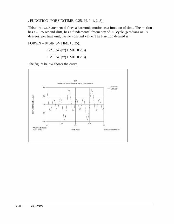
220 FORSIN
, FUNCTION=FORSIN(TIME,-0.25, PI, 0, 1, 2, 3)
This MOTION statement defines a harmonic motion as a function of time. The motionhas a -0.25 second shift, has a fundamental frequency of 0.5 cycle (p radians or 180degrees) per time unit, has no constant value. The function defined is:
FORSIN = 0+SIN(p*(TIME+0.25))
+2*SIN(2p*(TIME+0.25))
+3*SIN(3p*(TIME+0.25))
The figure below shows the curve.
FX 221
FX
Definition
The FX function returns the x-component of the net translational force acting atmarker i, as computed in the coordinate system of marker k. All force elementsacting between markers i and j are included in the calculation of the force, unless theforce is an action-only type force. To return the x-component of the action-onlyforces acting at marker i, you should omit specification of markers j and k or specifythem to be zero.
Format
FX(i[,j ][,k])
Arguments
i An integer that specifies the identifier of the marker at which the magnitudeof the net force is to be calculated.
j A second integer that specifies a marker identifier. All forces acting betweenthe [i,j] pair are to be included in the calculation. Set j = 0 or do not specify itif you are interested in action-only forces.
k An integer that specifies the identifier of a marker (coordinate system) inwhich the x-component of the force is to be returned. k defaults to the globalcoordinate system when it is not specified.
Examples
FX(23,0,432)
This extracts the x-component of the sum of all the action-only forces acting atMarker 23. The x-axis of Marker 432 specifies the direction along which the nettranslation force is computed.
222 FY
FY
Definition
The FY function returns the y-component of the net translational force acting atmarker i, as computed in the coordinate system of marker k. All force elementsacting between markers i and j are included in the calculation of the force, unless theforce is an action-only type force. To return the y-component of the action-onlyforces acting at marker i, you should omit specification of markers j and k or specifythem to be zero.
Format
FY(i[,j ][,k])
Arguments
i An integer that specifies the identifier of the marker at which the magnitudeof the net force is to be calculated.
j A second integer that specifies a marker identifier. All forces acting betweenthe [i,j] pair are to be included in the calculation. Set j = 0 or do not specify itif you are interested in action-only forces.
k An integer that specifies the identifier of a marker (coordinate system) inwhich the y-component of the force is to be returned. k defaults to the globalcoordinate system when it is not specified.
Examples
-0.3*FY(677,866)
This statement calculates a value -0.3 times the y-component of the net force along
the global y-axis, acting at Marker 677. All forces acting between Markers 677 and866 are included in this calculation.
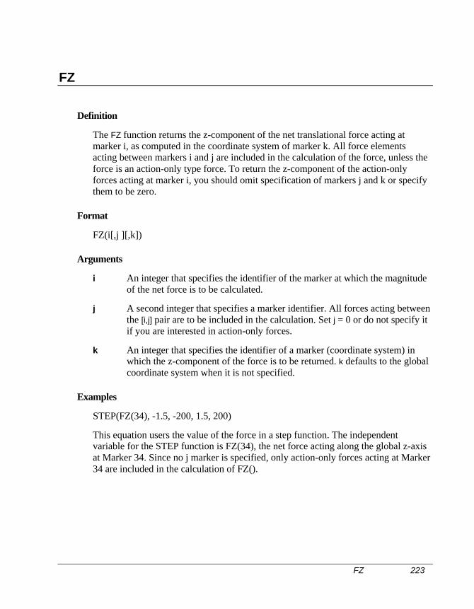
FZ 223
FZ
Definition
The FZ function returns the z-component of the net translational force acting atmarker i, as computed in the coordinate system of marker k. All force elementsacting between markers i and j are included in the calculation of the force, unless theforce is an action-only type force. To return the z-component of the action-onlyforces acting at marker i, you should omit specification of markers j and k or specifythem to be zero.
Format
FZ(i[,j ][,k])
Arguments
i An integer that specifies the identifier of the marker at which the magnitudeof the net force is to be calculated.
j A second integer that specifies a marker identifier. All forces acting betweenthe [i,j] pair are to be included in the calculation. Set j = 0 or do not specify itif you are interested in action-only forces.
k An integer that specifies the identifier of a marker (coordinate system) inwhich the z-component of the force is to be returned. k defaults to the globalcoordinate system when it is not specified.
Examples
STEP(FZ(34), -1.5, -200, 1.5, 200)
This equation users the value of the force in a step function. The independentvariable for the STEP function is FZ(34), the net force acting along the global z-axisat Marker 34. Since no j marker is specified, only action-only forces acting at Marker34 are included in the calculation of FZ().
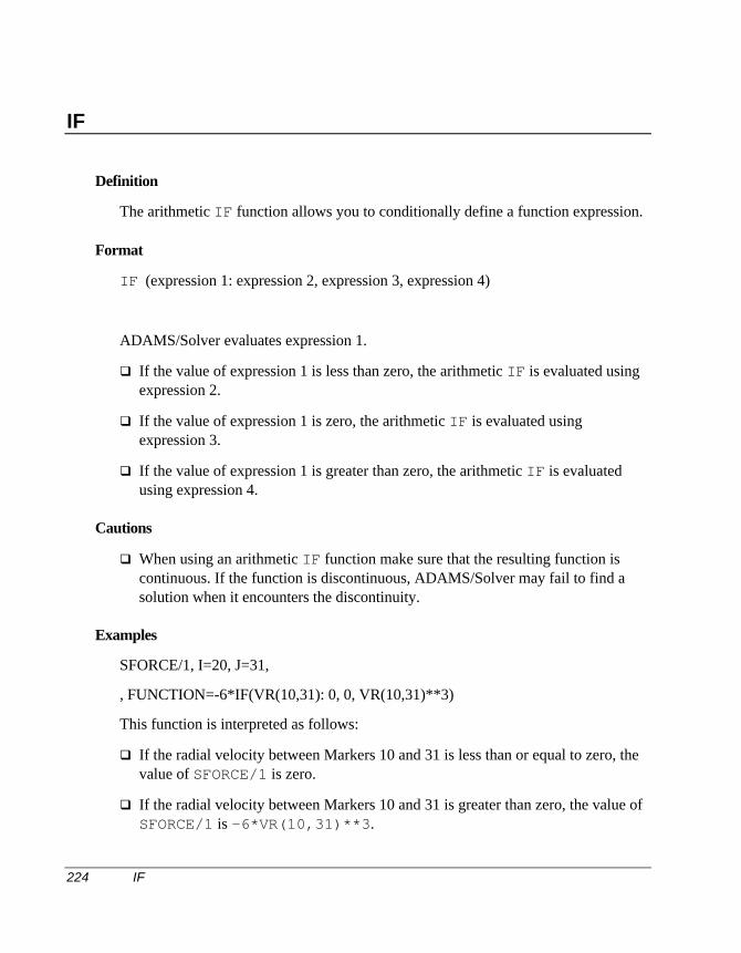
224 IF
IF
Definition
The arithmetic IF function allows you to conditionally define a function expression.
Format
IF (expression 1: expression 2, expression 3, expression 4)
ADAMS/Solver evaluates expression 1.
q If the value of expression 1 is less than zero, the arithmetic IF is evaluated usingexpression 2.
q If the value of expression 1 is zero, the arithmetic IF is evaluated usingexpression 3.
q If the value of expression 1 is greater than zero, the arithmetic IF is evaluatedusing expression 4.
Cautions
q When using an arithmetic IF function make sure that the resulting function iscontinuous. If the function is discontinuous, ADAMS/Solver may fail to find asolution when it encounters the discontinuity.
Examples
SFORCE/1, I=20, J=31,
, FUNCTION=-6*IF(VR(10,31): 0, 0, VR(10,31)**3)
This function is interpreted as follows:
q If the radial velocity between Markers 10 and 31 is less than or equal to zero, thevalue of SFORCE/1 is zero.
q If the radial velocity between Markers 10 and 31 is greater than zero, the value ofSFORCE/1 is -6*VR(10,31)**3.
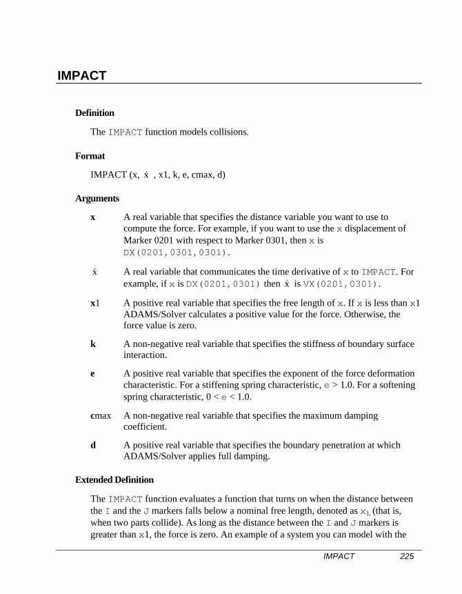
IMPACT 225
IMPACT
Definition
The IMPACT function models collisions.
Format
IMPACT (x, x& , x1, k, e, cmax, d)
Arguments
x A real variable that specifies the distance variable you want to use tocompute the force. For example, if you want to use the x displacement ofMarker 0201 with respect to Marker 0301, then x isDX(0201,0301,0301).
x& A real variable that communicates the time derivative of x to IMPACT. Forexample, if x is DX(0201,0301) then x& is VX(0201,0301).
x1 A positive real variable that specifies the free length of x. If x is less than x1ADAMS/Solver calculates a positive value for the force. Otherwise, theforce value is zero.
k A non-negative real variable that specifies the stiffness of boundary surfaceinteraction.
e A positive real variable that specifies the exponent of the force deformationcharacteristic. For a stiffening spring characteristic, e > 1.0. For a softeningspring characteristic, 0 < e < 1.0.
cmax A non-negative real variable that specifies the maximum dampingcoefficient.
d A positive real variable that specifies the boundary penetration at whichADAMS/Solver applies full damping.
Extended Definition
The IMPACT function evaluates a function that turns on when the distance betweenthe I and the J markers falls below a nominal free length, denoted as x1, (that is,when two parts collide). As long as the distance between the I and J markers isgreater than x1, the force is zero. An example of a system you can model with the
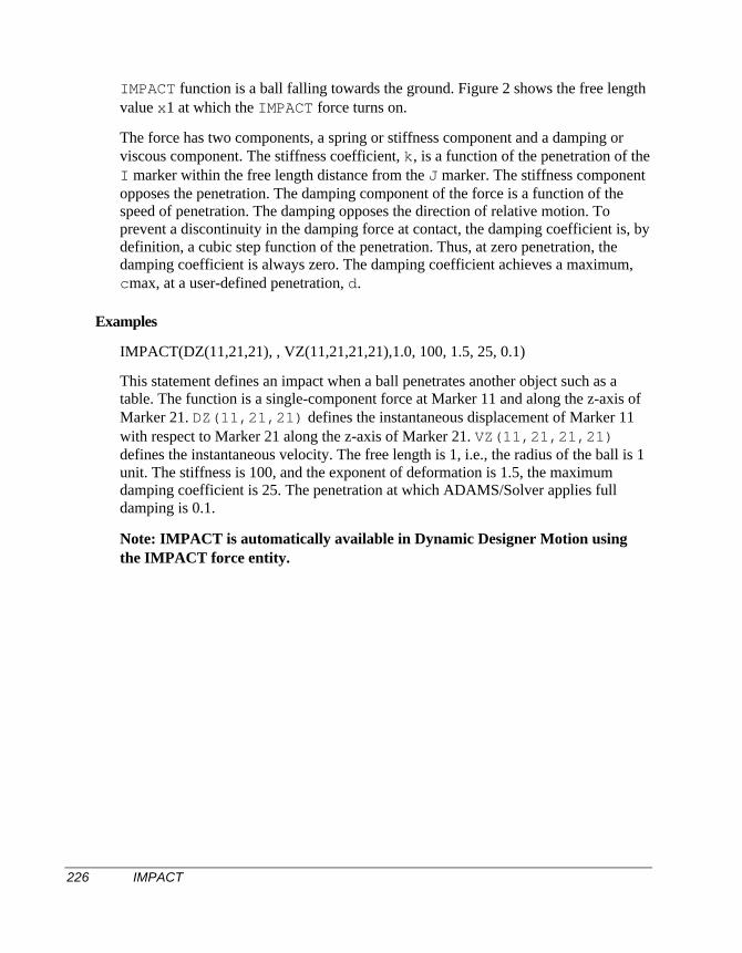
226 IMPACT
IMPACT function is a ball falling towards the ground. Figure 2 shows the free lengthvalue x1 at which the IMPACT force turns on.
The force has two components, a spring or stiffness component and a damping orviscous component. The stiffness coefficient, k, is a function of the penetration of theI marker within the free length distance from the J marker. The stiffness componentopposes the penetration. The damping component of the force is a function of thespeed of penetration. The damping opposes the direction of relative motion. Toprevent a discontinuity in the damping force at contact, the damping coefficient is, bydefinition, a cubic step function of the penetration. Thus, at zero penetration, thedamping coefficient is always zero. The damping coefficient achieves a maximum,cmax, at a user-defined penetration, d.
Examples
IMPACT(DZ(11,21,21), , VZ(11,21,21,21),1.0, 100, 1.5, 25, 0.1)
This statement defines an impact when a ball penetrates another object such as atable. The function is a single-component force at Marker 11 and along the z-axis ofMarker 21. DZ(11,21,21) defines the instantaneous displacement of Marker 11with respect to Marker 21 along the z-axis of Marker 21. VZ(11,21,21,21)defines the instantaneous velocity. The free length is 1, i.e., the radius of the ball is 1unit. The stiffness is 100, and the exponent of deformation is 1.5, the maximumdamping coefficient is 25. The penetration at which ADAMS/Solver applies fulldamping is 0.1.
Note: IMPACT is automatically available in Dynamic Designer Motion usingthe IMPACT force entity.
LOG 227
LOG
Definition
The LOG function returns the natural logarithm an expression a. If ex=a thenLOG(a)= x. The LOG function is defined only for positive values of a (i.e., a > 0). Itis undefined for all other values.
Format
LOG(a)
Arguments
a - Any valid function expression.
Examples
DIFF/1, IC=3.6
, FUNCTION=LOG(1+VM(21,31,31))
This DIFF statement defines a user specified differential equation. The initialcondition for the associated state is 3.6 and its derivative is the natural logarithm ofthe expression 1+VM(21,31,31).
228 LOG10
LOG10
Definition
The LOG10 function returns log to base 10 of an expression a. If 10x=a, thenLOG10(a)= x. The LOG10 function is defined only for positive values of a (i.e., a> 0). It is undefined for all other values.
Format
LOG10(a)
Arguments
a - Any valid function expression.
Examples
DIFF/1, IC=3.6
, FUNCTION=LOG10(1+VM(21,31,31))
This DIFF statement defines a user specified differential equation. The initialcondition for the associated state is 3.6 and its derivative is the natural logarithm ofthe expression 1+VM(21,31,31).
MAX 229
MAX
Definition
The MAX function returns the maximum of two expressions a1 and a2.
MAX(a1,a2) = a1 if a1 a2
MAX(a1,a2) = a2 if a2 > a1
Format
MAX(a1,a2)
Arguments
a1 - Any valid function expression.
a2 - Any valid function expression.
Cautions
q The MAX function is generally discontinuous. Use this function expression withcare when you are specifying force or motion input.
Examples
SFORCE/1, ROTATIONAL, ACTIONONLY, I=21, J=11
, FUNCTION=MAX(0,-3*(AZ(21,11)-25D))
This SFORCE statement defines an action-only torque that acts at Marker 21 and actsalong the z-axis of Marker 11. The torque is defined to always be non-negativethrough the use of the MAX function. Thus, the torque can only act to increase the AZrotation of Marker 21 with respect to Marker 11.
230 MIN
MIN
Definition
The MIN function returns the minimum of two expressions a1 and a2.
MIN(a1,a2) = a1 if a1 a2
MIN(a1,a2) = a2 if a2 < a1
Format
MIN(a1,a2)
Arguments
a1 - Any valid function expression.
a2 - Any valid function expression.
Cautions
q The MIN function is generally discontinuous. Use this function expression withcare when you are specifying force or motion input.
Examples
SFORCE/1, ROTATIONAL, ACTIONONLY, I=21, J=11
, FUNCTION=MIN(0,-3*(AZ(21,11)-25D))
This SFORCE statement defines an action-only torque that acts at Marker 21 and actsalong the z-axis of Marker 11. The torque is defined to always be negative throughthe use of the MIN function. Thus, the torque can only act to decrease the AZ rotationof Marker 21 with respect to Marker 11.
MOD 231
MOD
Definition
The MOD function returns the remainder when a1 is divided by a2.
MOD(a1,a2) = a1 - int(a1/a2) * a2
Format
MOD(a1,a2)
Arguments
a1 - Any valid function expression.
a2 - Any valid function expression.
Cautions
q The MOD function is generally discontinuous. Use this function expression withcare when you are specifying force or motion input.
Examples
MOD(45,16)=13
232 MOTION
MOTION
Definition
The MOTION function returns component comp of a force due to MOTION/id ascalculated in the coordinate system of marker rm. If jflag is set to zero, the valuereturned is the force/torque acting on the I marker of the MOTION. If jflag is set toone, the value returned is that acting on the J marker. rm may be specified as zero ifthe results are desired in the global coordinate system.
Format
MOTION (id, jflag, comp, rm)
Arguments
id An integer specifying the identification number of the motion.
jflag An integer flag specifying the motion connectivity marker at which theforces and torques are computed.0 = forces and moments at the I marker1 = forces and moments at the J marker
comp An integer value that specifies the component of the motion force to bereturned.1 = Magnitude of the force2 = x component of the force3 = y component of the force4 = z component of the force5 = Magnitude of the torque6 = x component of the torque7 = y component of the torque8 = z component of the torque
rm The coordinate system in which the results are expressed. To return theresults in the global coordinate system, set rm = 0.
ExamplesWZ(21,11)*MOTION(1,0,8,11)
This statement calculates the instantaneous power of MOTION/1 about the z-axisduring a simulation (Power = force * velocity).
PHI 233
PHI
Definition
The PHI function calculates the third angle (in radians) of a body-2 [313] Eulerrotation sequence between markers i and j. Marker j defaults to the globalcoordinate system if it is not specified.
Format
PHI(i[,j])
Arguments
i The marker whose rotations are being sought.
j The marker with respect to which the rotations are being measured.
Examples
PHI(222,434)
This function returns the phi angle between Markers 222 and 434 in its secondcolumn.
234 PI
PI
Definition
PI returns the ratio of the circumference of a circle to its diameter (3.14159...).
Format
PI
PITCH 235
PITCH
Definition
Calculates the second angle of a Body-3 [3 -2 1] yaw-pitch-roll rotation sequencebetween marker i and j. Marker j defaults to the global coordinate system if it isnot specified. Note that pitch is an Euler angle.
Format
PITCH(i[,j])
Arguments
i The marker whose rotations are being sought.
j The marker with respect to which the rotations are being measured.
Examples
PITCH(143)
This function returns the pitch angle (in radians) of Marker 143 relative to the globalcoordinate system.
236 POLY
POLY
Definition
The POLY function evaluates a standard polynomial at a user-specified value x.
Format
POLY (x, x0, a0, a1,..., a30)
Arguments
x - A real variable that specifies the independent variable. For example, if theindependent variable in the function is time, x is the system variable TIME.
x0 - A real variable that specifies a shift in the polynomial.
a0,a1,...,a30 - The real variables that define as many as thirty-one coefficients for thepolynomial series.
Extended Definition
The POLY function evaluates a standard polynomial at a user-specified value x.x0,a0,a1,...,a30 are parameters used to define the constants for the polynomial. Thestandard polynomial is defined as:
P(x) = aj (x-x0)j
= a0 + a1 * (x-x0) + a2 * (x-x0)2 +...+ an * (x-x0)n
The index j has a range from zero to n, where n is the number of terms in the series.
Examples
MOTION/1, JOINT=21, TRANSLATION
, FUNCTION=POLY(TIME, 0, 0, 0, 1)
This MOTION statement uses a quadratic polynomial function with respect to thesystem variable TIME to define a motion. That expanded function is:
Poly = time2
POLY 237
MOTION/1, JOINT=21, TRANSLATION
, FUNCTION = IF(TIME-5: 0, 0, POLY(TIME, 5, 0, 10))
This MOTION statement uses an arithmetic IF in its function expression to switchbetween functions.
The expanded function is:
if (time - 5) then Poly=0
else Poly=10*time-5
SFORCE/3, I=10, J=20, TRANSLATION
, FUNCTION=-POLY(DM(10, 20), 10, 0, 25, 0, 0.75)
This SFORCE statement defines a force with a nonlinear force deformationcharacteristic. This relationship is:
Poly=-25*[DM(10,20)-10]+ 0.75*[DM(10,20)-10]3,
where, DM(10,20) represents the magnitude of the displacement of Marker 10 withrespect to Marker 20. The free length of the spring is 10 units.
238 PSI
PSI
Definition
The PSI function expression calculates the first angle (in radians) of a body-2 [313]Euler rotation sequence between markers i and j. Marker j defaults to the globalcoordinate system if it is not specified.
Format
PSI(i[,j])
Arguments
i The marker whose rotations are being sought.
j The marker with respect to which the rotations are being measured.
Examples
PSI(222,434)
This function returns the psi angle between Markers 222 and 434 in its secondcolumn.
ROLL 239
ROLL
Definition
The ROLL function calculates the third angle of a Body-3 [3 -2 1] yaw-pitch-rollrotation sequence between markers i and j. Marker j defaults to the globalcoordinate system if it is not specified. Note that roll is an Euler angle.
Format
ROLL(i[,j])
Arguments
i The marker whose rotations are being sought.
j The marker with respect to which the rotations are being measured.
Examples
ROLL(143)
This function returns the roll angle (in radians) of Marker 143 relative to the globalcoordinate system.
240 RTOD
RTOD
Definition
RTOD returns the radians to degrees conversion factor.
Format
RTOD
Examples
REQUEST/1, F2=ROLL(23,14)*RTOD
This REQUEST statement outputs the roll angle between Markers 23 and 14 indegrees.
SHF 241
SHF
Definition
The SHF function evaluates a simple harmonic function. The following equationdefines SHF.
SHF = a*sin(ω*(x-x0)-phi)+b
Format
SHF (x, x0, a, w, phi, b)
Arguments
x - The independent variable in the function. It may be any value of interest to you sothat you can compute the value using the function expression. For example, if theindependent variable in the function is time, x is the system variable TIME.
x0 - The offset in the independent variable x.
a - The amplitude of the harmonic function.
w - The frequency of the harmonic function. ADAMS/Solver assumes w is in radiansper unit of the independent variable. Conversion to degrees per unit of theindependent is achieved by appending a D after the number specifying w.
phi - A phase shift in the harmonic function. ADAMS/Solver assumes phi is inradians unless you use a D after the value.
b - The average value of displacement of the harmonic function.
Examples
SHF(TIME, 25D, PI, 360D, 0, 5)
This MOTION statement uses SHF to define the harmonic function:
SHF = 5+PI*sin(360D*(time-25D))
The motion has a shift of 25 degrees, has an amplitude of PI, has a frequency of1 cycle (360D) per time unit, has zero phase shift, and has an average value ofdisplacement of 5 units.
242 SIGN
SIGN
Definition
The SIGN function transfers the sign of a2 to the magnitude of a1.
SIGN(a1,a2) = ABS(a1) if a2 0
SIGN(a1,a2) = -ABS(a1) if a2 < 0
Format
SIGN (a1,a2)
Arguments
a1 - Any valid function expression.
a2 - Any valid function expression.
Cautions
q The SIGN function is discontinuous. Use this function with care to avoid creatingexpressions that are discontinuous.
Examples
VARIABLE/23, FUNCTION=10*SIGN(DM(24,33),VZ(24,33))
When VZ(24,33) ³ 0, the value of VARIABLE/23 is -10*DM(24,33). WhenVZ(24,33) < 0, the value of VARIABLE/23 is 10*DM(24,33).
SIN 243
SIN
Definition
The SIN function returns the sine of an expression a.
Format
SIN(a)
Arguments
a - Any valid function expression.
Examples
SFORCE/1, TRANSLATION, I=23, J=34
, FUNCTION=SIN(10*TIME)
A translational force is defined to be acting along the line joining Markers 23 and 34.The force at Marker 23 is defined to be SIN(10*TIME).
244 SINH
SINH
Definition
The SINH function return the hyperbolic sine of an expression a.
SINH(a) = (ea-e-a) / 2.0
Format
SINH(a)
Arguments
a - Any valid function expression.
Examples
VARIABLE/1, FUNCTION=SINH(DX(21,32))
The value of VARIABLE/1 is the hyperbolic sine of the x-component of thedisplacement between Markers 21 and 32, as calculated in the global coordinatesystem.
SQRT 245
SQRT
Definition
The SQRT function returns the square root of an expression a. The square rootfunction is defined only for non-negative values of the argument a.
Format
SQRT(a)
Arguments
a - Any valid function expression.
246 STEP
STEP
Definition
The STEP function approximates the Heaviside step function with a cubicpolynomial. It has continuous first derivatives. Its second derivatives arediscontinuous at x=x0 and x=x1.
FormatSTEP (x, x0, h0, x1, h1)
Arguments
x - The independent variable.
x0 - A real variable that specifies the x value at which the STEP function begins.
x1 - A real variable that specifies the x value at which the STEP function ends.
h0 - The initial value of the step.
h1 - The final value of the step.
Extended Definition
The STEP function approximates the Heaviside step function with a cubicpolynomial. The figure below illustrates the STEP function.
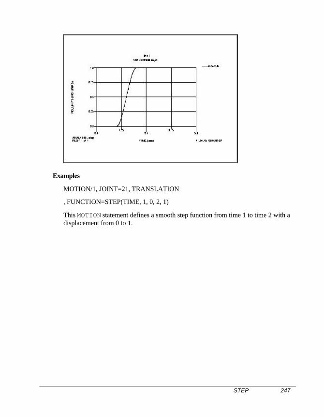
STEP 247
Examples
MOTION/1, JOINT=21, TRANSLATION
, FUNCTION=STEP(TIME, 1, 0, 2, 1)
This MOTION statement defines a smooth step function from time 1 to time 2 with adisplacement from 0 to 1.
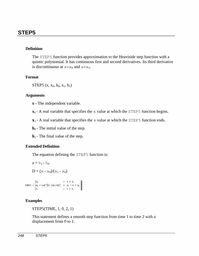
248 STEP5
STEP5
Definition
The STEP5 function provides approximation to the Heaviside step function with aquintic polynomial. It has continuous first and second derivatives. Its third derivativeis discontinuous at x=x0 and x=x1.
Format
STEP5 (x, x0, h0, x1, h1)
Arguments
x - The independent variable.
x0 - A real variable that specifies the x value at which the STEP5 function begins.
x1 - A real variable that specifies the x value at which the STEP5 function ends.
h0 - The initial value of the step.
h1 - The final value of the step.
Extended Definition
The equation defining the STEP5 function is:
a = h1 - h0
D = (x - x0)/(x1 - x0)
Examples
STEP5(TIME, 1, 0, 2, 1)
This statement defines a smooth step function from time 1 to time 2 with adisplacement from 0 to 1.
TAN 249
TAN
Definition
The TAN function returns the tangent of an expression a.
Format
TAN(a)
Arguments
a - Any valid function expression.
250 TANH
TANH
Definition
The TANH function returns the hyperbolic tangent of an expression a.
TANH(a)= (ea - e-a) / (ea + e-a)
Format
TANH(a)
Arguments
a - Any valid function expression.
Examples
MOTION/1, JOINT=21, TRANSLATION
, FUNCTION=0.5(1+TANH(5*(TIME-1.5)))
This MOTION statement defines a smooth step function that transitions from a valueof 0 to 1. The value of the step function at time=1.5 is 0.5.
THETA 251
THETA
Definition
The THETA function calculates the second angle (in radians) of a body-2 [313] Eulerrotation sequence between markers i and j. Marker j defaults to the globalcoordinate system if it is not specified.
Format
THETA(i[,j])
Arguments
i The marker whose rotations are being sought.
j The marker with respect to which the rotations are being measured.
Examples
THETA(222,434)
This function returns the psi angle between Markers 222 and 434.
252 TIME
TIME
Definition
The TIME variable returns the current simulation time.
Format
TIME
Examples
SFORCE/1, TRANSLATION, I=21, J=32
, FUNCTION=10*SIN(2*PI*TIME)
This SFORCE statement defines a translational force acting between the origins ofMarker 21 and Marker 11. The value of the force is 10*SIN*(2*PI*TIME).
TM 253
TM
Definition
The TM function returns the magnitude of the net torque acting at marker i due to allapplied torques and constraints acting between markers i and j. To calculate themagnitude of the net torque at marker i due to action-only torque acting at i, set j = 0.
Format
TM(i[,j])
Arguments
i An integer that specifies the identifier of the marker at which the magnitudeof the net torque is to be calculated.
j A second integer that specifies a marker identifier. All torques actingbetween the [i,j] pair are to be included in the calculation. Set j = 0 or do notspecify it if you are interested in action-only torques.
ExamplesJOINT/1, REVOLUTE, I=32, J=44MOTION/1, ROTATION, JOINT=1, FUNCTION=10*TIMEVARIABLE/31, FUNCTION=TM(32,44)
In this example a revolute joint and motion (through the joint) act between Marker 32and 44. A new algebraically determined state variable VARIABLE/31 is defined tohave the magnitude of the net torque between these two markers as its value.
254 TX
TX
Definition
The TX function returns the x-component of the net torque acting at marker i, ascomputed in the coordinate system of marker k. All force elements acting betweenmarkers i and j are included in the calculation of the torque, unless the force elementis an action-only type force. To return the x-component of the action-only torquesacting at marker i, you should omit specification of marker j or specify it as zero.
Format
TX(i[,j][,k])
Arguments
i An integer that specifies the identifier of the marker at which the magnitudeof the net torque is to be calculated.
j A second integer that specifies a marker identifier. All torques actingbetween the [i,j] pair are to be included in the calculation. Set j = 0 or do notspecify it if you are interested in action-only torques.
k An integer that specifies the identifier of a marker (coordinate system) inwhich the x-component of the torque is to be returned.
ExamplesJOINT/1, REVOLUTE, I=32, J=44MOTION/1, ROTATION, JOINT=1, FUNCTION=10*TIMEVARIABLE/31, FUNCTION=TX(32,44)
In this example a revolute joint and motion (through the joint) act between Marker 32and 44. A new algebraically determined state variable VARIABLE/31 is defined tohave the magnitude of the net torque between these two markers as its value.
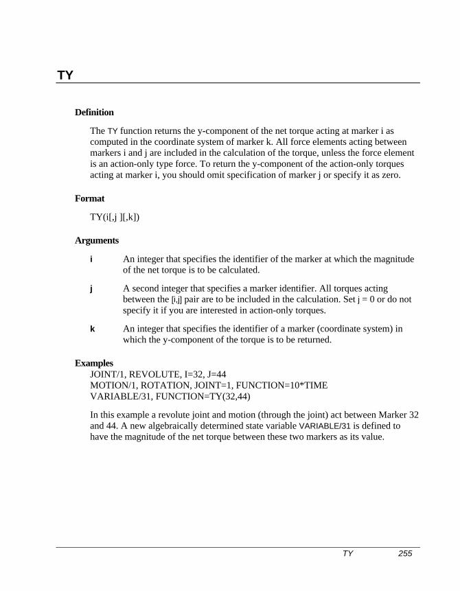
TY 255
TY
Definition
The TY function returns the y-component of the net torque acting at marker i ascomputed in the coordinate system of marker k. All force elements acting betweenmarkers i and j are included in the calculation of the torque, unless the force elementis an action-only type force. To return the y-component of the action-only torquesacting at marker i, you should omit specification of marker j or specify it as zero.
Format
TY(i[,j ][,k])
Arguments
i An integer that specifies the identifier of the marker at which the magnitudeof the net torque is to be calculated.
j A second integer that specifies a marker identifier. All torques actingbetween the [i,j] pair are to be included in the calculation. Set j = 0 or do notspecify it if you are interested in action-only torques.
k An integer that specifies the identifier of a marker (coordinate system) inwhich the y-component of the torque is to be returned.
ExamplesJOINT/1, REVOLUTE, I=32, J=44MOTION/1, ROTATION, JOINT=1, FUNCTION=10*TIMEVARIABLE/31, FUNCTION=TY(32,44)
In this example a revolute joint and motion (through the joint) act between Marker 32and 44. A new algebraically determined state variable VARIABLE/31 is defined tohave the magnitude of the net torque between these two markers as its value.

256 TZ
TZ
Definition
The TZ function returns the z-component of the net torque acting at marker i ascomputed in the coordinate system of marker k. All force elements acting betweenmarkers i and j are included in the calculation of the torque, unless the force elementis an action-only type force. To return the z-component of the action-only torquesacting at marker i, you should omit specification of marker j or specify it as zero.
Format
TZ(i[,j ][,k])
Arguments
i An integer that specifies the identifier of the marker at which the magnitudeof the net torque is to be calculated.
j A second integer that specifies a marker identifier. All torques actingbetween the [i,j] pair are to be included in the calculation. Set j = 0 or do notspecify it if you are interested in action-only torques.
k An integer that specifies the identifier of a marker (coordinate system) inwhich the z-component of the torque is to be returned.
ExamplesJOINT/1, REVOLUTE, I=32, J=44MOTION/1, ROTATION, JOINT=1, FUNCTION=10*TIMEVARIABLE/31, FUNCTION=TZ(32,44)
In this example a revolute joint and motion (through the joint) act between Marker 32and 44. A new algebraically determined state variable VARI ABLE/ 31 is defined tohave the magnitude of the net torque between these two markers as its value.
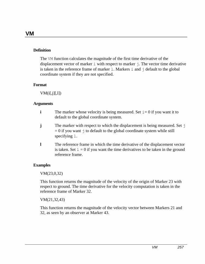
VM 257
VM
Definition
The VM function calculates the magnitude of the first time derivative of thedisplacement vector of marker i with respect to marker j. The vector time derivativeis taken in the reference frame of marker l. Markers i and j default to the globalcoordinate system if they are not specified.
Format
VM(i[,j][,l])
Arguments
i The marker whose velocity is being measured. Set i= 0 if you want it todefault to the global coordinate system.
j The marker with respect to which the displacement is being measured. Set j= 0 if you want j to default to the global coordinate system while stillspecifying l.
l The reference frame in which the time derivative of the displacement vectoris taken. Set l = 0 if you want the time derivatives to be taken in the groundreference frame.
Examples
VM(23,0,32)
This function returns the magnitude of the velocity of the origin of Marker 23 withrespect to ground. The time derivative for the velocity computation is taken in thereference frame of Marker 32.
VM(21,32,43)
This function returns the magnitude of the velocity vector between Markers 21 and32, as seen by an observer at Marker 43.
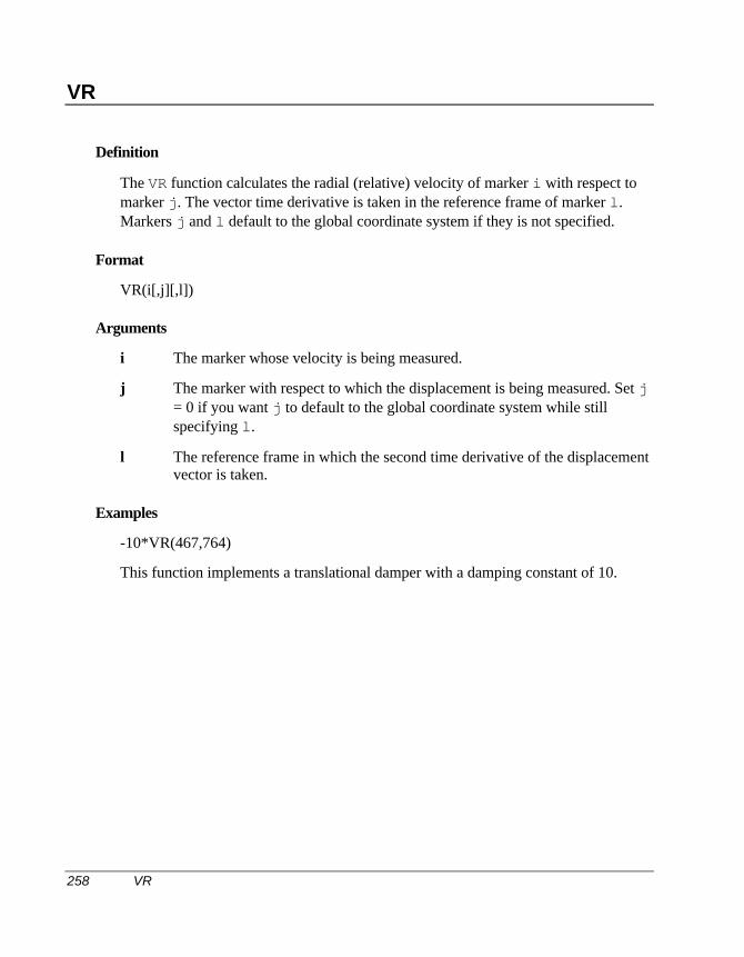
258 VR
VR
Definition
The VR function calculates the radial (relative) velocity of marker i with respect tomarker j. The vector time derivative is taken in the reference frame of marker l.Markers j and l default to the global coordinate system if they is not specified.
Format
VR(i[,j][,l])
Arguments
i The marker whose velocity is being measured.
j The marker with respect to which the displacement is being measured. Set j= 0 if you want j to default to the global coordinate system while stillspecifying l.
l The reference frame in which the second time derivative of the displacementvector is taken.
Examples
-10*VR(467,764)
This function implements a translational damper with a damping constant of 10.
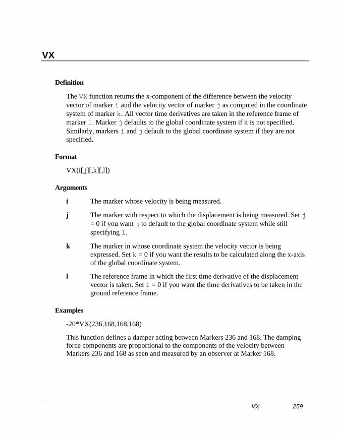
VX 259
VX
Definition
The VX function returns the x-component of the difference between the velocityvector of marker i and the velocity vector of marker j as computed in the coordinatesystem of marker k. All vector time derivatives are taken in the reference frame ofmarker l. Marker j defaults to the global coordinate system if it is not specified.Similarly, markers i and j default to the global coordinate system if they are notspecified.
Format
VX(i[,j][,k][,l])
Arguments
i The marker whose velocity is being measured.
j The marker with respect to which the displacement is being measured. Set j= 0 if you want j to default to the global coordinate system while stillspecifying l.
k The marker in whose coordinate system the velocity vector is beingexpressed. Set k = 0 if you want the results to be calculated along the x-axisof the global coordinate system.
l The reference frame in which the first time derivative of the displacementvector is taken. Set l = 0 if you want the time derivatives to be taken in theground reference frame.
Examples
-20*VX(236,168,168,168)
This function defines a damper acting between Markers 236 and 168. The dampingforce components are proportional to the components of the velocity betweenMarkers 236 and 168 as seen and measured by an observer at Marker 168.
260 VY
VY
Definition
The VY function returns the y-component of the difference between the velocityvector of marker i and the velocity vector of marker j as computed in the coordinatesystem of marker k. All vector time derivatives are taken in the reference frame ofmarker l. Marker j defaults to the global coordinate system if it is not specified.Similarly, markers i and j default to the global coordinate system if they are notspecified.
Format
VY(i[,j][,k][,l])
Arguments
i The marker whose velocity is being measured.
j The marker with respect to which the displacement is being measured. Set j= 0 if you want j to default to global coordinate system while stillspecifying l.
k The marker in whose coordinate system the velocity vector is beingexpressed. Set k = 0 if you want the results to be calculated along the x-axisof the global coordinate system.
l The reference frame in which the first time derivative of the displacementvector is taken. Set l = 0 if you want the time derivatives to be taken in theground reference frame.
Examples
-15*VY(236,168,168,168)
VZ 261
VZ
Definition
The VZ function returns the z-component of the difference between the velocityvector of marker i and the velocity vector of marker j as computed in the coordinatesystem of marker k. All vector time derivatives are taken in the reference frame ofmarker l. Marker j defaults to the global coordinate system if it is not specified.Similarly, markers i and j default to the global coordinate system if they are notspecified.
Format
VZ(i[,j][,k][,l])
Arguments
i The marker whose velocity is being measured.
j The marker with respect to which the displacement is being measured. Set j= 0 if you want j to default to global coordinate system while stillspecifying l.
k The marker in whose coordinate system the velocity vector is beingexpressed. Set k = 0 if you want the results to be calculated along the x-axisof the global coordinate system.
l The reference frame in which the first time derivative of the displacementvector is taken. Set l = 0 if you want the time derivatives to be taken in theground reference frame.
Examples
-20*VZ(236,168,168,168)
262 WDTM
WDTM
Definition
The WDTM function returns the magnitude of the difference between the angularacceleration vector of marker i in the reference frame of marker l and the angularacceleration of marker j in the reference frame of marker l.
Format
WDTM(i[,j ][,l])
Arguments
i The marker whose acceleration is being measured.
j The marker with respect to which the acceleration is being measured. Set j =0, while still specifying l, if you want j default to the global coordinatesystem.
l The reference frame in which the first time derivative of the angular velocityvector is taken. Set l = 0 if you want the time derivatives to be taken in theground reference frame.
Examples
WDTM(1236,2169)
This function obtains the angular acceleration magnitude of Marker 1236 withrespect to Marker 2169, as seen in the global coordinate system and measured in theground reference frame.

WDTX 263
WDTX
Definition
The WDTX function returns the x-component of the difference between the angularacceleration vector of marker i in the reference frame of marker l and the angularacceleration vector of marker j in the reference frame of marker l, as computed in thecoordinate system of marker k. Marker j defaults to global coordinate system if it isnot specified. Similarly, marker k and l default to global coordinate system if they arenot specified.
Format
WDTX(i[,j][,k][,l ])
Arguments
i The marker whose acceleration is being measured.
j The marker with respect to which the acceleration is being measured. Set j =0, while still specifying l, if you want j to default to the global coordinatesystem.
k The marker in whose coordinate system the acceleration vector is beingexpressed. Set k = 0 if you want the results to be calculated along the x-axisof the global coordinate system.
l The reference frame in which the first time derivative of the angularacceleration vector is taken. Set l = 0 if you want the time derivatives to betaken in the ground reference frame.
Examples
F2=WDTX(1236,2169,2169,2169)
This function obtains the x-component of angular acceleration on Marker 1236 withrespect to Marker 2169, as seen in the global coordinate system of Marker 2169 andmeasured in the reference frame containing Marker 2169.
264 WDTY
WDTY
Definition
The WDTY function returns the y-component of the difference between the angularacceleration vector of marker i in the reference frame of marker l and the angularacceleration vector of marker j in the reference frame of marker l, as computed in thecoordinate system of marker k. Marker j defaults to the global coordinate system if itis not specified. Similarly, marker k and l default to the global coordinate system ifthey are not specified.
Format
WDTY(i[,j][,k][,l ])
Arguments
i The marker whose acceleration is being measured.
j The marker with respect to which the acceleration is being measured. Set j =0, while still specifying l, if you want j to default to the global coordinatesystem.
k The marker in whose coordinate system the acceleration vector is beingexpressed. Set k = 0 if you want the results to be calculated along the y-axisof the global coordinate system.
l The reference frame in which the first time derivative of the angularacceleration vector is taken. Set l = 0 if you want the time derivatives to betaken in the ground reference frame.
Examples
WDTY(1236,2169,2169,2169)
This function obtains the y-component of angular acceleration on Marker 1236 withrespect to Marker 2169, as seen in the global coordinate system of Marker 2169 andmeasured in the reference frame containing Marker 2169.
WDTZ 265
WDTZ
Definition
The WDTZ function returns the z-component of the difference between the angularacceleration vector of marker i in the reference frame of marker l and the angularacceleration vector of marker j in the reference frame of marker l, as computed in thecoordinate system of marker k. Marker j defaults to the global coordinate system if itis not specified. Similarly, marker k and l default to the global coordinate if they arenot specified.
Format
WDTZ(i[,j ][,k][,l])
Arguments
i The marker whose acceleration is being measured.
j The marker with respect to which the acceleration is being measured. Set j =0, while still specifying l, if you want j to default to the global coordinatesystem.
k The marker in whose coordinate system the acceleration vector is beingexpressed. Set k = 0 if you want the results to be calculated along the z-axisof the global coordinate system.
l The reference frame in which the first time derivative of the angularacceleration vector is taken. Set l = 0 if you want the time derivatives to betaken in the ground reference frame.
Examples
WDTZ(1236,2169,2169,2169)
This function obtains the z-component of angular acceleration on Marker 1236 withrespect to Marker 2169, as seen in the global coordinate system of Marker 2169 andmeasured in the reference frame containing Marker 2169.
266 WM
WM
Definition
The WM function returns the magnitude of the angular velocity vector ofmarker i with respect to marker j. Marker j defaults to the global coordinate systemif it is not specified.
Format
WM(i[,j])
Arguments
i The marker whose velocity is being measured.
j The marker with respect to which the displacement is being measured. Set j= 0 if you want j to default to the global coordinate system while stillspecifying l.
Examples
WM(1236,2169)
This function returns the magnitude of the angular velocity vector of Marker 1236and Marker 2169.

WX 267
WX
Definition
The WX function returns the x-component of the difference between the angularvelocity vector of marker i in ground and the angular velocity vector of marker j inground, and expressed in the coordinate system of marker k. Marker j defaults to theglobal coordinate system if it is not specified. Similarly, marker k defaults to theglobal coordinate system if it is not specified.
Format
WX(i[,j][,k])
Arguments
i The marker whose velocity is being measured.
j The marker with respect to which the displacement is being measured. Set j= 0 if you want j to default to the global coordinate system while stillspecifying l.
k The marker in whose coordinate system the velocity vector is beingexpressed. Set k = 0 if you want the results to be calculated along the x-axisof the global coordinate system.
Examples
WX(1236,2169,2169)
This function returns the x-component of the angular velocity Markers 1236 and2169 as measured in the coordinate system of Marker 2169.
268 WY
WY
Definition
The WY function returns the y-component of the difference between the angularvelocity vector of marker i in ground and the angular velocity vector of marker j inground, and expressed in the coordinate system of marker k. Marker j defaults to theglobal coordinate system if it is not specified. Similarly, marker k defaults to theglobal coordinate system if it is not specified.
Format
WY(i[,j][,k])
Arguments
i The marker whose velocity is being measured.
j The marker with respect to which the displacement is being measured. Set j= 0 if you want j to default to the global coordinate system while stillspecifying l.
k The marker in whose coordinate system the velocity vector is beingexpressed. Set k = 0 if you want the results to be calculated along the x-axisof the global coordinate system.
Examples
WY(1236,2169,2169)
This function returns the y-component of the angular velocity Markers 1236 and2169 as measured in the coordinate system of Marker 2169.
WZ 269
WZ
Definition
The WZ function returns the z-component of the difference between the angularvelocity vector of marker i in ground and the angular velocity vector of marker j inground, and expressed in the coordinate system of marker k. Marker j defaults to theglobal coordinate system if it is not specified. Similarly, marker k defaults to theglobal coordinate system if it is not specified.
Format
WZ(i[,j][,k])
Arguments
i The marker whose velocity is being measured.
j The marker with respect to which the displacement is being measured. Set j= 0 if you want j to default to the global coordinate system while stillspecifying l.
k The marker in whose coordinate system the velocity vector is beingexpressed. Set k = 0 if you want the results to be calculated along the x-axisof the global coordinate system.
Examples
WZ(1236,2169,2169)
This function returns the z-component of the angular velocity Markers 1236 and2169 as measured in the coordinate system of Marker 2169.
270 YAW
YAW
Definition
The YAW function calculates the first angle of a Body-3 [3 -2 1] yaw-pitch-rollrotation sequence between markers i and j. Marker j defaults to the globalcoordinate system if it is not specified. Note that yaw is an Euler angle.
Format
YAW(i[,j])
Arguments
i The marker whose rotations are being sought.
j The marker with respect to which the rotations are being measured.
Examples
YAW(21,11)
This function returns the yaw angles between Markers 21 and 11.
Floating Licenses Background 271
Floating Licenses Background
The purpose of this chapter is to provide the step by step process needed to activate a licenseserver for Dynamic Designer and on how to set up Client sites to access this server. We willbe using the licensing software provided on the Dynamic Designer CD.
The licensing security is done using FlexLM software. It provides the ability to license one ormore licenses over a Network environment.
Only Dynamic Designer/Motion or Dynamic Designer/Motion Professional can be licensedover a network.
The License software only regulates licenses. Dynamic Designer must be installed on everyclient machine the product is to run on. You do not need to install Dynamic Designer on theserver machine (unless you want to use it on that machine).
When installing Dynamic Designer on Client Machines, use the serial number on the back ofthe CD provided in the shipment. This serial number is specifically for floating licenseinstallations and cannot be used to install a stand-alone version of Dynamic Designer.
11 Floating LicenseInstallation
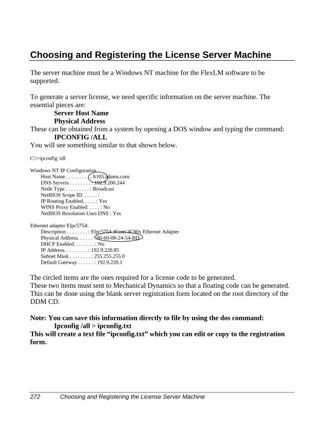
272 Choosing and Registering the License Server Machine
Choosing and Registering the License Server Machine
The server machine must be a Windows NT machine for the FlexLM software to besupported.
To generate a server license, we need specific information on the server machine. Theessential pieces are:
Server Host NamePhysical Address
These can be obtained from a system by opening a DOS window and typing the command:IPCONFIG /ALL
You will see something similar to that shown below.
C:\>ipconfig /all
Windows NT IP Configuration Host Name . . . . . . . . . : lt105.adams.com DNS Servers . . . . . . . . : 192.9.200.244 Node Type . . . . . . . . . : Broadcast NetBIOS Scope ID. . . . . . : IP Routing Enabled. . . . . : Yes WINS Proxy Enabled. . . . . : No NetBIOS Resolution Uses DNS : Yes
Ethernet adapter Elpc5754: Description . . . . . . . . : Elpc5754 3Com 3C90x Ethernet Adapter Physical Address. . . . . . : 00-60-08-24-54-BD DHCP Enabled. . . . . . . . : No IP Address. . . . . . . . . : 192.9.220.85 Subnet Mask . . . . . . . . : 255.255.255.0 Default Gateway . . . . . . : 192.9.220.1
The circled items are the ones required for a license code to be generated.These two items must sent to Mechanical Dynamics so that a floating code can be generated.This can be done using the blank server registration form located on the root directory of theDDM CD.
Note: You can save this information directly to file by using the dos command:Ipconfig /all > ipconfig.txt
This will create a text file “ipconfig.txt” which you can edit or copy to the registrationform.

Installation of Dynamic Designer Licensing Software 273
Installation of Dynamic Designer Licensing Software
From the Dynamic Designer CD, run setup.exe and select the INSTALL DYNAMICDESIGNER LICENSE SERVER option.
When the Installation Dialog appears, select the location where you would like the softwareinstalled. The default locations is C:\Program Files\Dynamic Designer License Server
Press the NEXT button when ready to continue.
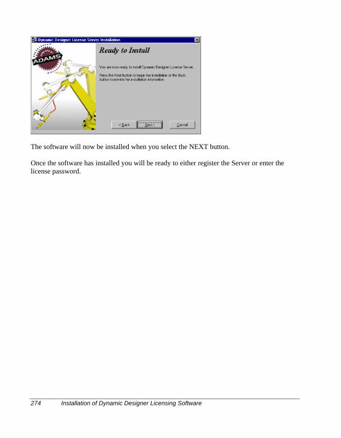
274 Installation of Dynamic Designer Licensing Software
The software will now be installed when you select the NEXT button.
Once the software has installed you will be ready to either register the Server or enter thelicense password.

Configuring a Dynamic Designer License Server 275
Configuring a Dynamic Designer License Server
There are two ways to license the server:By reading a saved password certificate fileManually keying in the codes needed
Creating a License by Reading from the Password Certificate file
Before starting a License Server, you need to have received your Distribution RequestAuthorization code (Password Certificate). This is in the from of an email that looks like thetext shown below. Unless you wish to manually go through entering information line by line,the fastest way to get the server license is to save a portion the email to a file and then loadthat into the license software.
- If you are installing new passwords, follow this procedure: 1) Verify that you are currently running on the ADAMS license server system. 2) If you have an ADAMS license server running, you must stop the license server by choosing (6) "Stop the ADAMS license server(s)". 3) Choose (4) "Install ADAMS passwords on this license server". 4) Choose (5) "Start the ADAMS license server on this system".
If you experience problems while installing these passwords, refer to theTroubleshooting section of the Installation Instructions.------------------- Cut Here ------------------- Cut Here --------------------;Start of Network License Information. (DO NOT REMOVE)SERVER lt105 0060082454BD 1986DAEMON adamsd {Installation Will Update This Information}FEATURE DT_SE_MOTIONPRO_2000P adamsd 10.0 15-AUG-2004 1\ 9C9220E13A4E9B998259 VENDOR_STRING="MDI" HOSTID=""FEATURESET adamsd 0D9796BD7D59E443;End of Network License Information. (DO NOT REMOVE)------------------- Cut Here ------------------- Cut Here --------------------
The portion of the email between the Cut Here lines above contains the licensing information.This is the only important portion of the email necessary in the file that you save (use anextension like .TXT, eg serverlicense.txt).
When saving this portion of the distribution request, put it somewhere very easy to find, e.g.C:\, c:\temp etc.
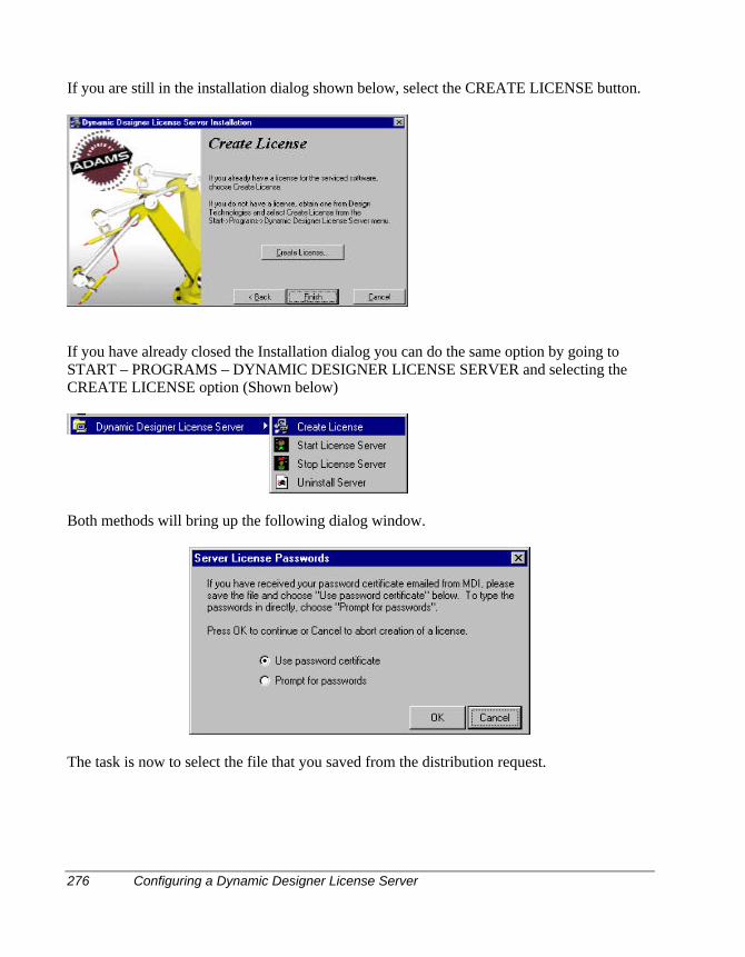
276 Configuring a Dynamic Designer License Server
If you are still in the installation dialog shown below, select the CREATE LICENSE button.
If you have already closed the Installation dialog you can do the same option by going toSTART – PROGRAMS – DYNAMIC DESIGNER LICENSE SERVER and selecting theCREATE LICENSE option (Shown below)
Both methods will bring up the following dialog window.
The task is now to select the file that you saved from the distribution request.
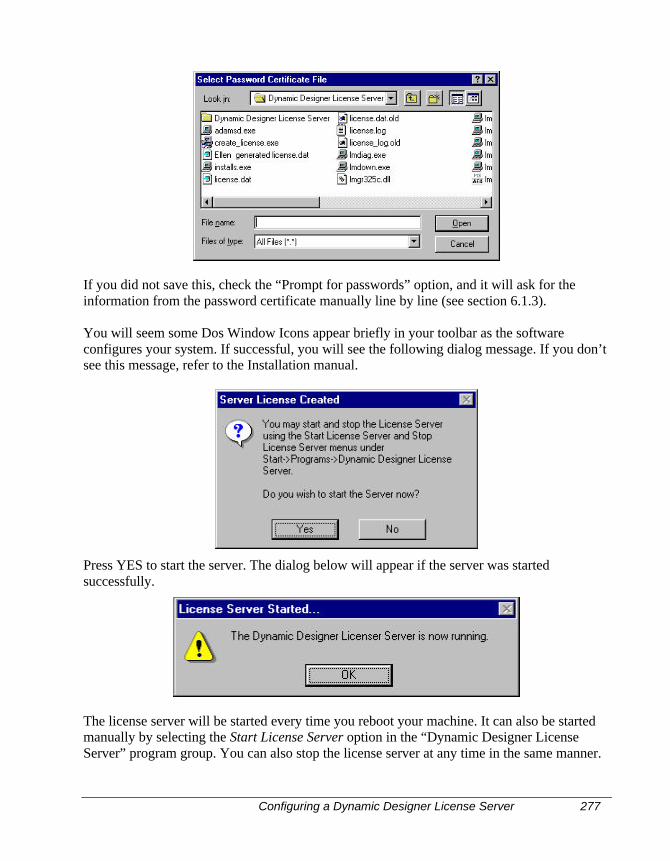
Configuring a Dynamic Designer License Server 277
If you did not save this, check the “Prompt for passwords” option, and it will ask for theinformation from the password certificate manually line by line (see section 6.1.3).
You will seem some Dos Window Icons appear briefly in your toolbar as the softwareconfigures your system. If successful, you will see the following dialog message. If you don’tsee this message, refer to the Installation manual.
Press YES to start the server. The dialog below will appear if the server was startedsuccessfully.
The license server will be started every time you reboot your machine. It can also be startedmanually by selecting the Start License Server option in the “Dynamic Designer LicenseServer” program group. You can also stop the license server at any time in the same manner.
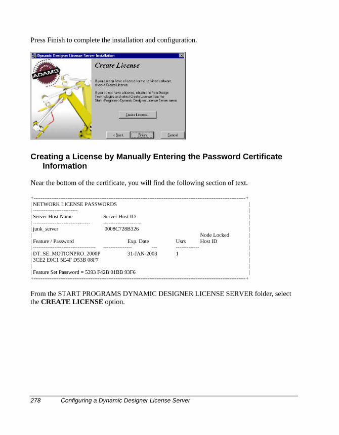
278 Configuring a Dynamic Designer License Server
Press Finish to complete the installation and configuration.
Creating a License by Manually Entering the Password CertificateInformation
Near the bottom of the certificate, you will find the following section of text.
+-----------------------------------------------------------------------------------------------------------------------+| NETWORK LICENSE PASSWORDS || ------------------------- || Server Host Name Server Host ID || -------------------------------- --------------------- || junk_server 0008C728B326 || Node Locked || Feature / Password Exp. Date Usrs Host ID || ----------------------------------- ---------------- --- ------------- || DT_SE_MOTIONPRO_2000P 31-JAN-2003 1 || 3CE2 E0C1 5E4F D53B 08F7 || || Feature Set Password = 5393 F42B 01BB 93F6 |+-----------------------------------------------------------------------------------------------------------------------+
From the START PROGRAMS DYNAMIC DESIGNER LICENSE SERVER folder, selectthe CREATE LICENSE option.
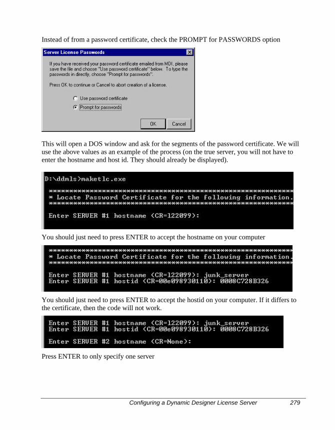
Configuring a Dynamic Designer License Server 279
Instead of from a password certificate, check the PROMPT for PASSWORDS option
This will open a DOS window and ask for the segments of the password certificate. We willuse the above values as an example of the process (on the true server, you will not have toenter the hostname and host id. They should already be displayed).
You should just need to press ENTER to accept the hostname on your computer
You should just need to press ENTER to accept the hostid on your computer. If it differs tothe certificate, then the code will not work.
Press ENTER to only specify one server
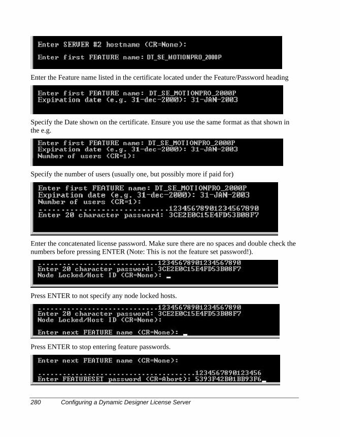
280 Configuring a Dynamic Designer License Server
Enter the Feature name listed in the certificate located under the Feature/Password heading
Specify the Date shown on the certificate. Ensure you use the same format as that shown inthe e.g.
Specify the number of users (usually one, but possibly more if paid for)
Enter the concatenated license password. Make sure there are no spaces and double check thenumbers before pressing ENTER (Note: This is not the feature set password!).
Press ENTER to not specify any node locked hosts.
Press ENTER to stop entering feature passwords.
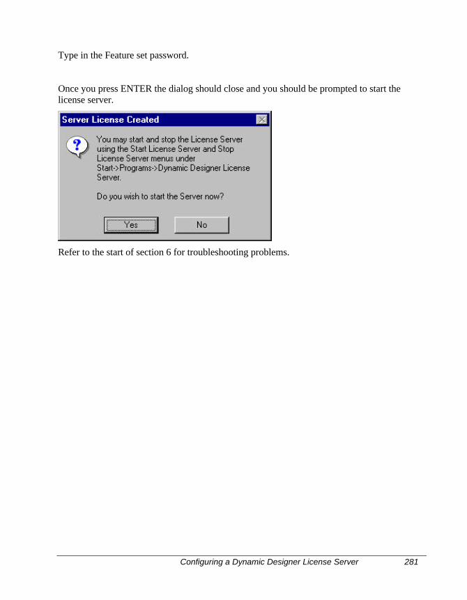
Configuring a Dynamic Designer License Server 281
Type in the Feature set password.
Once you press ENTER the dialog should close and you should be prompted to start thelicense server.
Refer to the start of section 6 for troubleshooting problems.
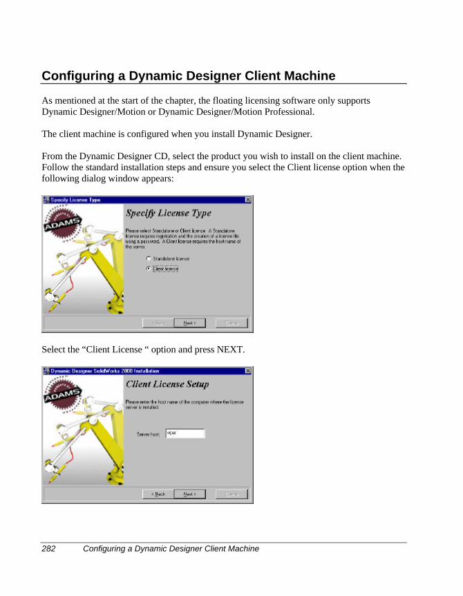
282 Configuring a Dynamic Designer Client Machine
Configuring a Dynamic Designer Client Machine
As mentioned at the start of the chapter, the floating licensing software only supportsDynamic Designer/Motion or Dynamic Designer/Motion Professional.
The client machine is configured when you install Dynamic Designer.
From the Dynamic Designer CD, select the product you wish to install on the client machine.Follow the standard installation steps and ensure you select the Client license option when thefollowing dialog window appears:
Select the “Client License “ option and press NEXT.

Configuring a Dynamic Designer Client Machine 283
Type in the name of the server that is licensing Dynamic Designer. If you are not sure, pleasecontact the systems administrator.
You should now be ready to run Dynamic Designer using a network license. If when you runDynamics Designer on the client machine, you are prompted for an authorization code, readthe error message displayed. If this message indicates that the server or feature cannot belocated, go through the trouble shooting section next in this chapter.
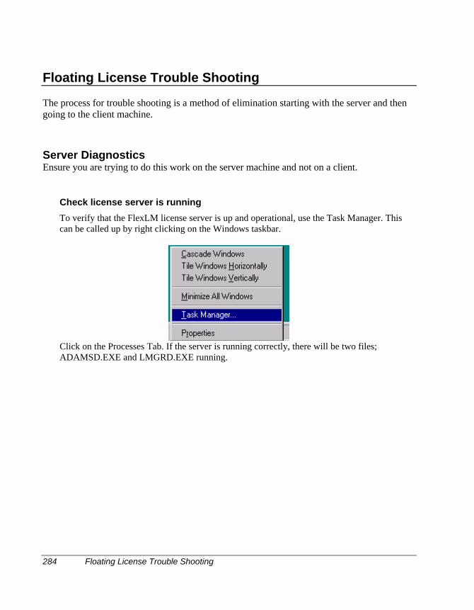
284 Floating License Trouble Shooting
Floating License Trouble Shooting
The process for trouble shooting is a method of elimination starting with the server and thengoing to the client machine.
Server DiagnosticsEnsure you are trying to do this work on the server machine and not on a client.
Check license server is running
To verify that the FlexLM license server is up and operational, use the Task Manager. Thiscan be called up by right clicking on the Windows taskbar.
Click on the Processes Tab. If the server is running correctly, there will be two files;ADAMSD.EXE and LMGRD.EXE running.
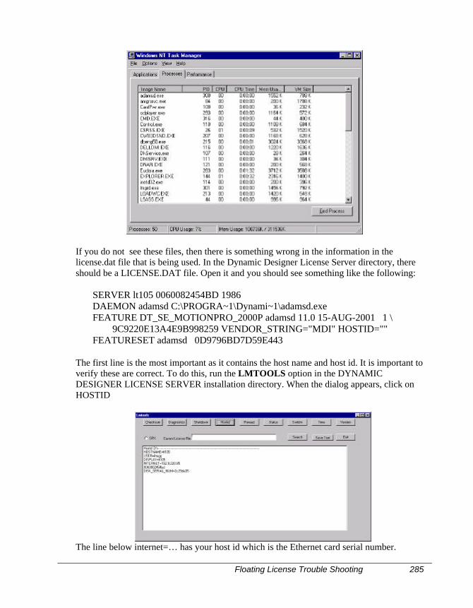
Floating License Trouble Shooting 285
If you do not see these files, then there is something wrong in the information in thelicense.dat file that is being used. In the Dynamic Designer License Server directory, thereshould be a LICENSE.DAT file. Open it and you should see something like the following:
SERVER lt105 0060082454BD 1986DAEMON adamsd C:\PROGRA~1\Dynami~1\adamsd.exeFEATURE DT_SE_MOTIONPRO_2000P adamsd 11.0 15-AUG-2001 1 \ 9C9220E13A4E9B998259 VENDOR_STRING="MDI" HOSTID=""FEATURESET adamsd 0D9796BD7D59E443
The first line is the most important as it contains the host name and host id. It is important toverify these are correct. To do this, run the LMTOOLS option in the DYNAMICDESIGNER LICENSE SERVER installation directory. When the dialog appears, click onHOSTID
The line below internet=… has your host id which is the Ethernet card serial number.
286 Floating License Trouble Shooting
Sometimes host names can contain characters not accepted by FlexLM, such as a dash (eg“lt105-ae1”. If you have a name like this, then it is recommended that you replace thehostname with the IP address for the computer. This is the number INTERNET=192.9.220.85as shown above.
Change the first line in the LICENSE.DAT to:SERVER 192.9.220.85 0060082454BD 1986
(Please make sure you use your own IP address and not the one shown here)
IMPORTANT NOTE: Whenever you make any changes to the license.dat file, you muststop the server and then restart it for the changes to take effect.
Once you have made these changes, please verify that ADAMSD.EXE and LMGRD.EXE arerunning by using the task manager as mentioned previously.
The next step in determining the cause for why the license server is not running correctly, isto look in the LICENSE.LOG file in the DYNAMIC DESIGNER LICENSE SERVERdirectory.
If everything works correctly, it should look like that shown below:
7:22:06 (adamsd) Logfile switched from stdout7:22:36 (adamsd) Server started on 192.9.220.85 for: DT_SE_MOTIONPRO_2000P7:24:34 (adamsd) OUT: " DT_SE_MOTIONPRO_2000P "Administrator@dt1547:47:51 (adamsd) IN: " DT_SE_MOTIONPRO_2000P "Administrator@dt154
This shows the server was started, and that someone had checked out (or used) a license offeature “DT_SE_MOTIONPRO_2000P” and then checked it back in.
If the license.log file does not contain any messages after starting the license server (i.e. it isblank), one of the common problems is if the password certificate file is corrupted. Thesolution to this is to manually enter the fields in the password certificate (prompt forpasswords option).
If the log file states that the service is not started, there will most likely be an error messageabove this line in the log file. If it is not clear what the error message is explaining, contactTechnical Support at Mechanical Dynamics ([email protected]), PH +1 734 214 9716,Fax +1 734 214 9717).Note: MDI headquarters works on US East Cost time.
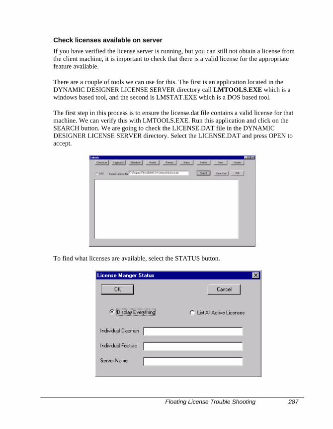
Floating License Trouble Shooting 287
Check licenses available on server
If you have verified the license server is running, but you can still not obtain a license fromthe client machine, it is important to check that there is a valid license for the appropriatefeature available.
There are a couple of tools we can use for this. The first is an application located in theDYNAMIC DESIGNER LICENSE SERVER directory call LMTOOLS.EXE which is awindows based tool, and the second is LMSTAT.EXE which is a DOS based tool.
The first step in this process is to ensure the license.dat file contains a valid license for thatmachine. We can verify this with LMTOOLS.EXE. Run this application and click on theSEARCH button. We are going to check the LICENSE.DAT file in the DYNAMICDESIGNER LICENSE SERVER directory. Select the LICENSE.DAT and press OPEN toaccept.
To find what licenses are available, select the STATUS button.
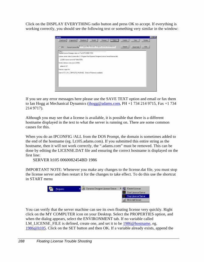
288 Floating License Trouble Shooting
Click on the DISPLAY EVERYTHING radio button and press OK to accept. If everything isworking correctly, you should see the following text or something very similar in the window:
If you see any error messages here please use the SAVE TEXT option and email or fax themto Ian Hogg at Mechanical Dynamics ([email protected], PH +1 734 214 9715, Fax +1 734214 9717).
Although you may see that a license is available, it is possible that there is a differenthostname displayed in the text to what the server is running on. There are some commoncauses for this.
When you do an IPCONFIG /ALL from the DOS Prompt, the domain is sometimes added tothe end of the hostname (eg. Lt105.adams.com). If you submitted this entire string as thehostname, then it will not work correctly, the “.adams.com” must be removed. This can bedone by editing the LICENSE.DAT file and ensuring the correct hostname is displayed on thefirst line:
SERVER lt105 0060082454BD 1986
IMPORTANT NOTE: Whenever you make any changes to the license.dat file, you must stopthe license server and then restart it for the changes to take effect. To do this use the shortcutin START menu
You can verify that the server machine can see its own floating license very quickly. Rightclick on the MY COMPUTER icon on your Desktop. Select the PROPERTIES option, andwhen the dialog appears, select the ENVIRONMENT tab. If no variable calledLM_LICENSE_FILE is defined, create one, and set it to be 1986@hostname, eg.1986@lt105. Click on the SET button and then OK. If a variable already exists, append the
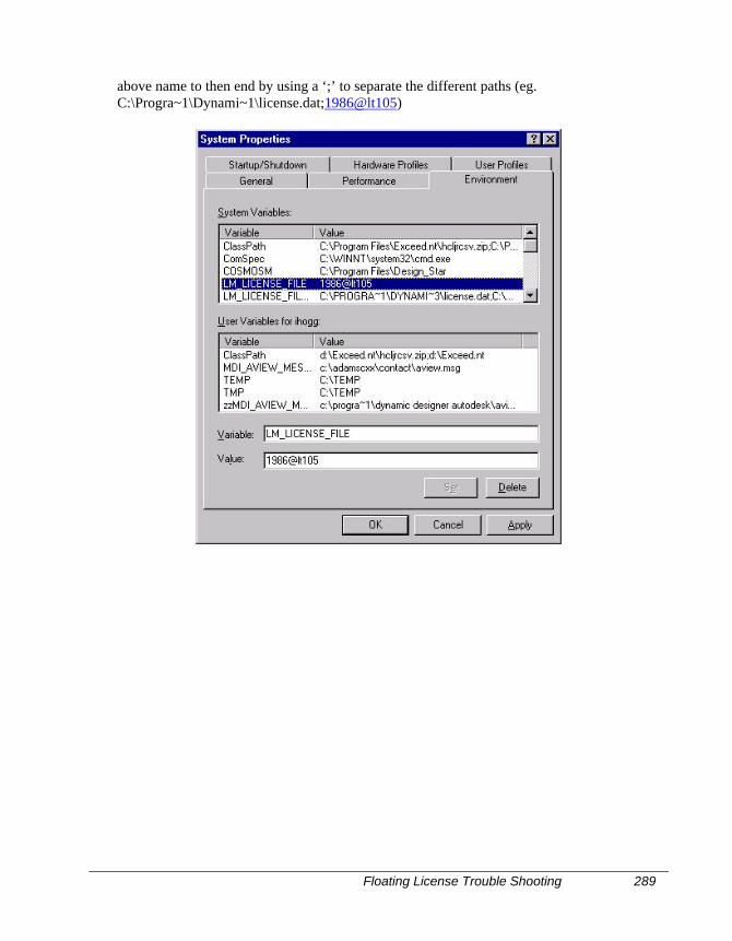
Floating License Trouble Shooting 289
above name to then end by using a ‘;’ to separate the different paths (eg.C:\Progra~1\Dynami~1\license.dat;1986@lt105)
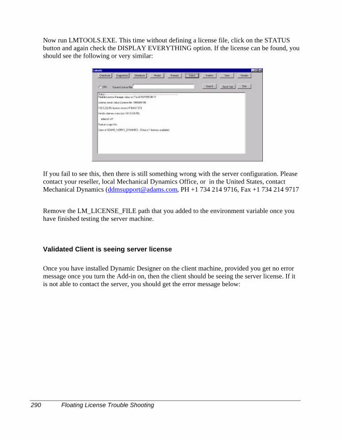
290 Floating License Trouble Shooting
Now run LMTOOLS.EXE. This time without defining a license file, click on the STATUSbutton and again check the DISPLAY EVERYTHING option. If the license can be found, youshould see the following or very similar:
If you fail to see this, then there is still something wrong with the server configuration. Pleasecontact your reseller, local Mechanical Dynamics Office, or in the United States, contactMechanical Dynamics ([email protected], PH +1 734 214 9716, Fax +1 734 214 9717
Remove the LM_LICENSE_FILE path that you added to the environment variable once youhave finished testing the server machine.
Validated Client is seeing server license
Once you have installed Dynamic Designer on the client machine, provided you get no errormessage once you turn the Add-in on, then the client should be seeing the server license. If itis not able to contact the server, you should get the error message below:
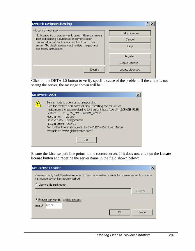
Floating License Trouble Shooting 291
Click on the DETAILS button to verify specific cause of the problem. If the client is notseeing the server, the message shown will be:
Ensure the License path line points to the correct server. If it does not, click on the Locatelicense button and redefine the server name in the field shown below:

292 Floating License Trouble Shooting
It is recommended after changing the hostname to close Solid Edge and re-run it, to ensure allchanges are recognized.
If you are sill unable to get the client machine to find a valid license on the server, verify oncemore that the server has a valid license. If the problem persists, please contact your reseller,local Mechanical Dynamics Office, or in the United States, Technical Support at MechanicalDynamics ([email protected], PH +1 734 214 9715, Fax +1 734 214
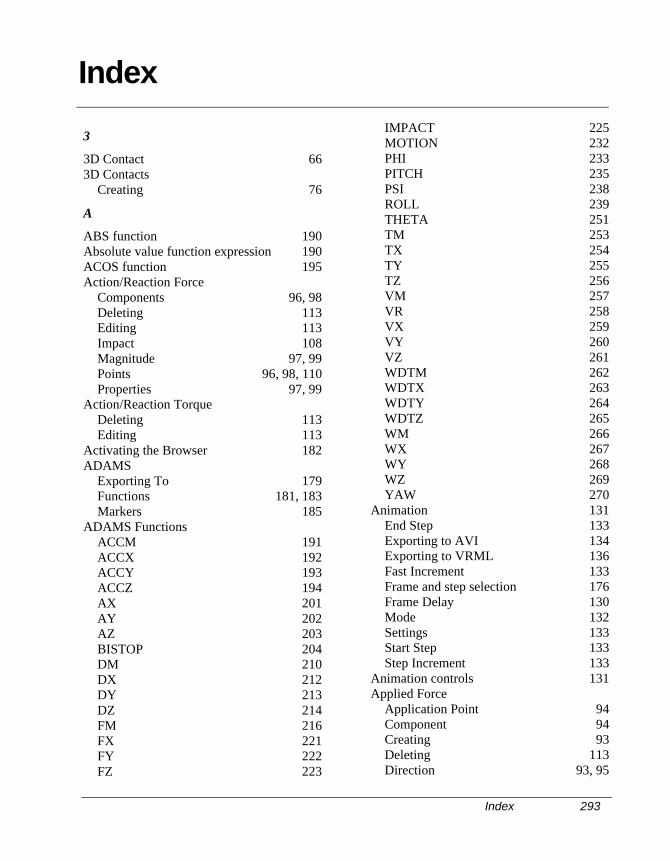
Index 293
3
3D Contact 663D Contacts
Creating 76
A
ABS function 190Absolute value function expression 190ACOS function 195Action/Reaction Force
Components 96, 98Deleting 113Editing 113Impact 108Magnitude 97, 99Points 96, 98, 110Properties 97, 99
Action/Reaction TorqueDeleting 113Editing 113
Activating the Browser 182ADAMS
Exporting To 179Functions 181, 183Markers 185
ADAMS FunctionsACCM 191ACCX 192ACCY 193ACCZ 194AX 201AY 202AZ 203BISTOP 204DM 210DX 212DY 213DZ 214FM 216FX 221FY 222FZ 223
IMPACT 225MOTION 232PHI 233PITCH 235PSI 238ROLL 239THETA 251TM 253TX 254TY 255TZ 256VM 257VR 258VX 259VY 260VZ 261WDTM 262WDTX 263WDTY 264WDTZ 265WM 266WX 267WY 268WZ 269YAW 270
Animation 131End Step 133Exporting to AVI 134Exporting to VRML 136Fast Increment 133Frame and step selection 176Frame Delay 130Mode 132Settings 133Start Step 133Step Increment 133
Animation controls 131Applied Force
Application Point 94Component 94Creating 93Deleting 113Direction 93, 95
Index
294 Index
Editing 113Properties 95Template Editor 95, 97, 99
Applied TorqueDeleting 113Editing 113
Arc tangent, calculating 199, 200ASIN function 198ATAN function 199ATAN2 function 200Automatically creating joints from mates 22AVI File 134
B
Bearing surfaces for FEA load distribution144
BrowserActivating 182
C
Cam Constraints 64Curve/Curve 65
Creating 69Curves 71Properties 72Tips 78
Point/Curve 64, 66Creating 67Point 68Properties 69Tips 78
Chebyshev polynomial, evaluating 205, 206Circle:calculating circumference 234Circumference, calculating 234Contact
3D 66Contacts
3DCreating 76
Converting:degrees to radians 211Converting:radians to degrees 240COS function 207COSH function 208Cosine, calculating 195, 207Couplers 79, 80
Coupling joint motion 79, 80Creating a VRML Animation File 136Creating an AVI Movie 134Creating XY Plots 160Cubic polynomial, using with function 246Curve/Curve Constraint 65
Creating 69Curves 71Properties 72Tips 78
D
Dampers 99Components 102Creating 102Deleting 113Editing 113Points 103
Data Points Function 92Degree conversion factor 211Degrees of freedom 16Deleting
XY Plots in Result Viewer 162Deleting Elements 113DOF Counter 124DTOR function 211Dynamic Designer/Motion
benefits of 2Registering 7
E
e value, calculating 215Editing Elements 113Excel 97 137Exporting Results to a Text File 140Exporting Results to Excel 97 137Exporting to ADAMS 179Exporting Trace Path coordinates 148Expressions
calculating maximum of two 229calculating minimum of two 230calculating remainder 231
F
FEA
Index 295
Bearing Surfaces 144Exporting To 143
Feature Tree 13Force
Applied Force 88Applied Torque 88Deleting 113Editing 113Gravity 88, 112Magnitude 88
Force MagnitudeTemplate Editor 88
Fourier cosine series, evaluating 217Fourier sine series, evaluating 219Friction
Cylindrical Joint 38Enabling Effects 36Joint Results 43Joints 35Planar Joint 42Revolute Joint 37Spherical Joint 39Translational Joint 40Universal Joint 41
Functions used in Expressions 181, 183
G
Gravity 112
H
Harmonic Function 90Heaviside step function, calculating246, 248Hyperbolic cosine, calculating 208Hyperbolic sine, calculating 244Hyperbolic tangent, calculating 250
I
Impact Forces 108Installation 3Interference Detection 141
J
Joint Couplers 79, 80Joint Primitives 44
Components 61Inline 45
Inplane 46Orientation 47Parallel Axes 48Pependicular 49Properties 62
JointsAutomatically create from mates 22Components 61Cylindrical 18, 29Cylindrical, Friction 38Definition 25Degrees of freedom 26Deleting 113Editing 113Fixed 34Hinge 17, 27Planar 33Planar, Friction 42Properties 62Results, Friction 43Revolute, Friction 37Screw 32Spherical 30Spherical, Friction 39Translational 28Translational, Friction 40Universal 31Universal, Friction 41
L
Log to base 10, calculating 228Logarithm, calculating natural 227
M
Magnitude, calculating nearest integer196,197
Markers 185Materials 115
Adding 115Editing 119
Model BuilderCommand 165Gravity Page 167Ground Parts Menu 176Joints Menu 172Joints Page 172
296 Index
Manually Adding Joints 173Motion Page 174Parts Page 168Rigidly Attaching Component 169Simulation Page 175Springs Menu 173Springs Page 175Units Page 166
Modeling power transmission elements79,80
Modeling Procedure 19, 20Motion Drivers 50
Defining 63Deleting 113Editing 113Function Expression 63Other Functions 57Template Editor 51Template Editor 52Template Editor 63Type 51
Motion PartsCreating 22Drag and Drop within the Browser 22Rigidly Attaching Parts 24
O
Output Steps 126
P
PlaybackMode 132
Point/Curve Constraint 64, 66Creating 67Point 68Properties 69Tips 78
Polynomial, evaluating standard 236Positive difference, calculating values 209
Q
Quintic polynomial, using with function 248
R
Radian conversion factor 240
Registration 7Results
Exporting to a Text File 140Exporting to Excel 97 137Exporting Trace Path coordinates 148Interference Detection 141Trace Paths 147
Rigid Bodydefinition 26ground 83mass properties 83
Rotational DriversDeleting 113Editing 113Template Editor 51, 52
Running a Simulation 129
S
Serial Number 4Sign, transferring to magnitude 242Simple harmonic function, evaluating 241Simulation
Output Steps 126Simulation
Animate during Simulation 127Animating 134Error Criteria 128Initial Time Step 128Integrator 128Maximum Iterations 128Maximum Time Step 128Minimum Time Step 128Running 129Settings 126, 127status 124Time 127Troubleshooting 130
Simulation PanelAnimation Controls 131Buttons 124DOF Counter 124Mode 124Step 125Time 125
Simulation Panel 123Simulation:returning current time 252
Index 297
Sine, calculating 243Springs 99
Components 100, 104Creating 100, 104, 106, 109Deleting 113Editing 113Points 101
Springs and Dampers 99Square root, calculating 245Step Function 89
T
Tangent, calculating 249Template Editor
Data Points Function 55, 92Expression 51Force Magnitude 88Harmonic Function 54, 90Motion Driver 51, 52Step Function 52, 89
Text File 140Torque Magnitude
Template Editor 88Torsion Dampers
Components 106, 109Creating 106, 109Deleting 113Editing 113Location 107Orientation 107
Torsion SpringsComponents 104
Creating 104Deleting 113Editing 113Location 105Orientation 105
Trace Paths 147Translational Driver
Deleting 113Editing 113Template Editor 51, 52
V
VRML File 136
X
XY Plots, Result ViewerAxes Properties 152Chart Properties 150Creating 160Deleting 162Double clicking on 162Fonts 154Gridlines 151Moving Marker Properties 158Numbers/Scale 155Plot Curve Properties 157Plot Defaults 149Plot Layout 150Plot Persistence 163X Axis options 160