DSANLS: Accelerating Distributed Nonnegative Matrix

Factorization via Sketching

Technical Report

Yuqiu Qian∗1, Conghui Tan†2, Nikos Mamoulis‡3, and David W. Cheung�1

1Department of Computer Science, The University of Hong Kong2Department of SEEM, The Chinese University of Hong Kong

3Department of Computer Science & Engineering, University of Ioannina

Abstract

Nonnegative matrix factorization (NMF) has been successfully applied in di�erent �elds,such as text mining, image processing, and video analysis. NMF is the problem of determiningtwo nonnegative low rank matrices U and V , for a given input matrix M , such that M ≈UV >. There is an increasing interest in parallel and distributed NMF algorithms, due tothe high cost of centralized NMF on large matrices. In this paper, we propose a distributed

sketched alternating nonnegative least squares (DSANLS) framework for NMF, which utilizesa matrix sketching technique to reduce the size of nonnegative least squares subproblems ineach iteration for U and V . We design and analyze two di�erent random matrix generationtechniques and two subproblem solvers. Our theoretical analysis shows that DSANLS convergesto the stationary point of the original NMF problem and it greatly reduces the computationalcost in each subproblem as well as the communication cost within the cluster. DSANLS isimplemented using MPI for communication, and tested on both dense and sparse real datasets.The results demonstrate the e�ciency and scalability of our framework, compared to the state-of-art distributed NMF MPI implementation. Its implementation is available at https://github.com/qianyuqiu79/DSANLS.

1 Introduction

Nonnegative matrix factorization (NMF) is a technique for discovering nonnegative latent factorsand/or performing dimensionality reduction. NMF �nds applications in text mining [34], im-age/video processing [21], and analysis of social networks [38]. Unlike general matrix factorization(MF), NMF restricts the two output matrix factors to be nonnegative. Nonnegativity is inherent inthe feature space of many real-world applications, therefore the resulting factors can have a naturalinterpretation. Speci�cally, the goal of NMF is to decompose a huge matrix M ∈ Rm×n

+ into the

∗yqqian@cs.hku.hk†chtan@se.cuhk.edu.hk‡nikos@cs.uoi.gr�dcheung@cs.hku.hk

1

product of two matrices U ∈ Rm×k+ and V ∈ Rn×k

+ such that M ≈ UV >. Rm×n+ denotes the set

of m × n matrices with nonnegative real values, and k is a user-speci�ed dimensionality, wheretypically k � m,n.

Generally, NMF can be de�ned as an optimization problem [23] as follows:

minU∈Rm×k

+ ,V ∈Rn×k+

∥∥∥M − UV >∥∥∥F, (1)

where ‖X‖F =(∑

ij x2ij

)1/2is the Frobenius norm of X. However, Problem (1) is hard to solve

directly because it is non-convex. Therefore, almost all NMF algorithms leverage two-block coordi-nate descent schemes. That is, they optimize just over one of the two factors, U or V , while keepingthe other �xed [8]. By �xing V , we can optimize U by solving a nonnegative least squares (NLS)subproblem:

minU∈Rm×k

+

∥∥∥M − UV >∥∥∥F. (2)

Modern data analysis tasks apply on big matrix data with increasing scale and dimensionality.Examples include community detection in a billion-node social network, background separation ona 4K video in which every frame has approximately 27 million rows [17], text mining on a bag-of-words matrix with millions of words. The volume of data is anticipated to increase in the `bigdata' era, making it impossible to store the whole matrix in the main memory throughout NMF.Therefore, there is a need for high-performance and scalable distributed NMF algorithms.

In this paper, we propose a distributed framework for NMF. We choose MPI1/C for our dis-tributed implementation for e�ciency, generality and privacy reasons. MPI/C does not requirereading/writing data to/from disk or global shu�es of data matrix entries, as Spark or MapReducedo. Nodes can collaborate without sharing their local input data, which is important for applicationsthat involve sensitive data and have privacy considerations. Besides, high performance numericalcomputing routines like MKL2 can be leveraged. The state-of-art implementation of distributedNMF is MPI-FAUN [17], a general framework that iteratively solves nonnegative least squares(NLS) subproblems for U and V . The main idea behind MPI-FAUN is to exploit the independenceof local updates for rows of U and V , in order to minimize the communication requirements ofmatrix multiplication operations within the NMF algorithms.

Our idea is to speed up distributed NMF in a new, orthogonal direction: by reducing the problemsize of each NLS subproblem within NMF, which in turn decreases the overall computation cost. Ina nutshell, we reduce the size of each NLS subproblem, by employing a matrix sketching technique:the involved matrices in the subproblem are multiplied by a specially designed random matrix ateach iteration, which greatly reduces their dimensionality. As a result, the computational cost ofeach subproblem drops.

However, applying matrix sketching comes with several issues. First, although the size of eachsubproblem is signi�cantly reduced, sketching involves matrix multiplication which brings compu-tational overhead. Second, unlike in a single machine setting, the data are distributed to di�erentnodes, which may have to communicate extensively in a poorly designed solution. In particular, eachnode only retains part of both the input matrix and the generated approximate matrices, causingdi�culties due to data dependencies in the computation process. Besides, the generated random

1Message Passing Interface2Intelr Math Kernel Library

2

matrices should be the same for all nodes in every iteration, while broadcasting the random matrixto all nodes brings severe communication overhead and can become the bottleneck of distributedNMF. Furthermore, after reducing each original subproblem to a sketched random new subproblem,it is not clear whether the algorithm still converges and whether it converges to stationary pointsof the original NMF problem.

Our distributed sketched alternating nonnegative least squares (DSANLS) overcomes these prob-lems. First, the extra computation cost due to sketching is reduced with a proper choice of therandom matrices. Second, the same random matrices used for sketching are generated indepen-dently at each node, thus there is no need for communication of random matrices between nodesduring distributed NMF. Having the complete random matrix at each node, an NMF iteration canbe done locally with the help of a matrix multiplication rule with proper data partitioning. There-fore, our matrix sketching approach reduces not only the computational, but also the communicationcost. Moreover, due to the fact that sketching also shifts the optimal solution of each original NMFsubproblem, we propose subproblem solvers paired with theoretical guarantees of their convergenceto a stationary point of the original subproblems.

Our contributions can be summarized as follows:

• We propose DSANLS, a novel high-performance distributed NMF algorithm. DSANLS is the�rst distributed NMF algorithm that leverages matrix sketching to reduce the problem sizeof each NLS subproblem and can be applied to both dense and sparse input matrices with aconvergence guarantee.

• We propose a novel and specially designed subproblem solver (proximal coordinate descent),which helps DSANLS to converge faster. We also discuss the use of projected gradient descent

as subproblem solver, showing that it is equivalent to stochastic gradient descent (SGD) onthe original (non-sketched) NLS subproblem.

• We present a detailed theoretical analysis of DSANLS, and prove that DSANLS converges to astationary point of the original NMF problem. This convergence proof is novel and non-trivialbecause of the involvement of matrix sketching at each iteration.

• We conduct an experimental evaluation using several (dense and sparse) real datasets, whichdemonstrates the e�ciency and scalability of DSANLS.

The remainder of the paper is organized as follows. Section 2 brie�y discusses the propertiesof NMF, reviews NMF algorithms and distributed NMF techniques, and introduces the matrixsketching technique. Our DSANLS algorithm is presented in Section 3. Detailed theoretical analysisof DSANLS algorithm is discussed in Section 4. Section 5 evaluates DSANLS. Finally, Section 6concludes the paper.

2 Background and Related Work

2.1 Properties of NMF

In this paper, we focus on solving problem (1), which has several properties. First, general NMFis NP-hard [41], so typical methods aim at �nding an approximate solution (i.e., a local optimum).The second property is that the search space of NMF has numerous local minimums, so the results ofdi�erent algorithms may vary signi�cantly [14]. Third, choosing the best value for the factorization

3

rank k is quite hard. Widely-used approaches are: trial and error, estimation using SVD, and theuse of experts' insights [43].

2.2 NMF Algorithms

Almost all NMF algorithms leverage a two-block coordinate descent scheme (exact or inexact). Thatis, they optimize just over one of the two factors, U or V , while keeping the other �xed [8]. Thereason is that the original problem (1) is non-convex, so it is hard to solve it directly. However, by�xing V , we can solve a convex subproblem:

minU∈Rm×k

+

∥∥∥M − UV >∥∥∥F, (3)

More precisely, (3) is a nonnegative least squares (NLS) problem. Similarly, if we �x U , the problembecomes:

minV ∈Rn×k

+

∥∥∥M> − V U>∥∥∥F. (4)

Algorithm 1: Two-Block Coordinate Descent: Framework of Most NMF Algorithms

initialize U0 ≥ 0, V0 ≥ 0;for t = 0 to T − 1 do

Ut+1 ← update(M , Ut, Vt);Vt+1 ← update(M , Ut+1, Vt);

end

return UT and VT

The �rst widely used update rule is Multiplicative Updates (MU), which was �rst applied forsolving NLS problems in [6]. Later, MU was rediscovered and used for NMF in [23]. MU is basedon the majorization-minimization framework. Its application guarantees that the objective functionmonotonically decreases [6, 23].

Another extensively studied method is alternating nonnegative least squares (ANLS), whichrepresents a class of methods where the subproblems for U and V are solved exactly following theframework described in Algorithm 1. ANLS is guaranteed to converge to a stationary point [11]and has been shown to perform very well in practice with active set [18, 20], projected gradient [26],quasi-Newton [46], or accelerated gradient [13] methods as the subproblem solver.

Hierarchical alternating least squares (HALS) [4] solves each NLS subproblem using an exactcoordinate descent method that updates one individual column of U at a time. The optimal solutionsof the corresponding subproblems can be written in a closed form.

2.3 Distributed NMF

Parallel NMF algorithms are well studied in the literature [15, 39]. However, di�erent from aparallel, single machine setting, in a distributed setting, data sharing and communication haveconsiderable cost. Therefore, we need specialized NMF algorithms for massive scale data handlingin a distributed environment. The �rst method in this direction [27] is based on the MU algorithm. Itmainly focuses on sparse matrices and applies a careful partitioning of the data in order to maximizedata locality and parallelism. Later, CloudNMF [25], a MapReduce-based NMF algorithm similar

4

to [27], was implemented and tested on large-scale biological datasets. Another distributed NMFalgorithm [45] leverages block-wise updates for local aggregation and parallelism. It also performsfrequent updates using whenever possible the most recently updated data, which is more e�cientthan traditional concurrent counterparts. Apart from MapReduce implementations, Spark is alsoattracting attention for its advantage in iterative algorithms, e.g., using MLlib [31]. Finally, thereare implementations using X10 [12] and on GPU [30].

The most recent and related work in this direction is MPI-FAUN [16, 17], which is the �rstimplementation of NMF using MPI for interprocessor communication. MPI-FAUN is �exible andcan be utilized for a broad class of NMF algorithms that iteratively solve NLS subproblems includingMU, HALS, and ANLS/BPP. MPI-FAUN exploits the independence of local update computationfor rows of U and V to apply communication-optimal matrix multiplication. In a nutshell, thefull matrix M is split across a two-dimensional grid of processors and multiple copies of both Uand V are kept at di�erent nodes, in order to reduce the communication between nodes during theiterations of NMF algorithms.

2.4 Matrix Sketching

Matrix sketching is a technique that has been previously used in numerical linear algebra [10],statistics [36] and optimization [37]. Its basic idea is described as follows. Suppose we need to �nda solution x to the equation:

Ax = b, (A ∈ Rm×n, b ∈ Rm). (5)

Instead of solving this equation directly, in each iteration of matrix sketching, a random matrixS ∈ Rd×m (d� m) is generated, and we instead solve the following problem:

(SA)x = Sb. (6)

Obviously, the solution of (5) is also a solution to (6), but not vice versa. However, the problemsize has now decreased from m × n to d × n. With a properly generated random matrix S andan appropriate method to solve subproblem (6), it can be guaranteed that we will progressivelyapproach the solution to (5) by iteratively applying this sketching technique.

To the best of our knowledge, there is only one piece of previous work [42] which incorporatesdual random projection into the NMF problem, in a centralized environment, sharing similar ideasas SANLS, the centralized version of our DSANLS algorithm. However, Wang et al. [42] didnot provide an e�cient subproblem solver, and their method was less e�ective than non-sketchedmethods in practical experiments. Besides, data sparsity was not taken into consideration in theirwork. Furthermore, no theoretical guarantee was provided for NMF with dual random projection.In short, SANLS is not same as [42] and DSANLS is much more than a distributed version of [42].The methods that we propose in this paper are e�cient in practice and have strong theoreticalguarantees.

3 DSANLS: Distributed Sketched ANLS

As opposed to ANLS-based methods, which compute an optimal solution for each NLS subproblem(as mentioned in Section 2.1), our Distributed Sketched ANLS approach reduces the size of eachNLS subproblem using matrix sketching and solves it approximately. We now present the details ofour method.

5

3.1 Notations

For a matrix A, we use Ai:j to denote the entry at the i-th row and j-th column of A. Besides,either i or j can be omitted to denote a column or a row, i.e., Ai: is the i-th row of A, and A:j

is its j-th column. Furthermore, i or j can be replaced by a subset of indices. For example, ifI ⊂ {1, 2, . . . ,m}, AI: denotes the sub-matrix of A formed by all rows in I, whereas A:J is thesub-matrix of A formed by all columns in a subset J ⊂ {1, 2, . . . , n}.

3.2 Data Partitioning

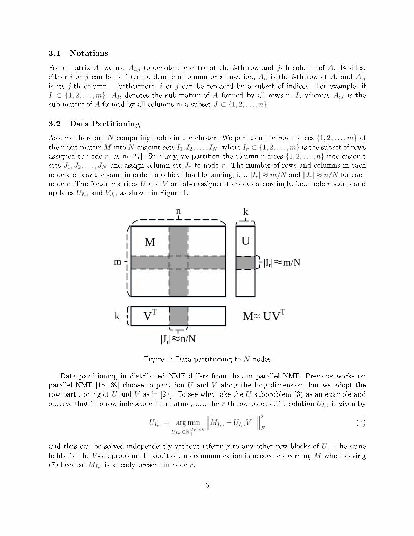
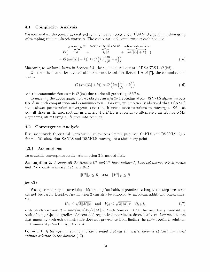
Assume there are N computing nodes in the cluster. We partition the row indices {1, 2, . . . ,m} ofthe input matrixM into N disjoint sets I1, I2, . . . , IN , where Ir ⊂ {1, 2, . . . ,m} is the subset of rowsassigned to node r, as in [27]. Similarly, we partition the column indices {1, 2, . . . , n} into disjointsets J1, J2, . . . , JN and assign column set Jr to node r. The number of rows and columns in eachnode are near the same in order to achieve load balancing, i.e., |Ir| ≈ m/N and |Jr| ≈ n/N for eachnode r. The factor matrices U and V are also assigned to nodes accordingly, i.e., node r stores andupdates UIr: and VJr: as shown in Figure 1.

m

n

k

k

|Jr| n/N

|Ir| m/N

M UVTVT

UM

Figure 1: Data partitioning to N nodes

Data partitioning in distributed NMF di�ers from that in parallel NMF. Previous works onparallel NMF [15, 39] choose to partition U and V along the long dimension, but we adopt therow-partitioning of U and V as in [27]. To see why, take the U -subproblem (3) as an example andobserve that it is row-independent in nature, i.e., the r-th row block of its solution UIr: is given by

UIr: = arg minUIr :∈R

|Ir |×k+

∥∥∥MIr: − UIr:V>∥∥∥2F

(7)

and thus can be solved independently without referring to any other row blocks of U . The sameholds for the V -subproblem. In addition, no communication is needed concerning M when solving(7) because MIr: is already present in node r.

6

On the other hand, solving (7) requires the entire V of size n×k, meaning that every node needsto gather V from all other nodes. This process can easily be the bottleneck of a naive distributedANLS implementation. As we will explain shortly, our DSALNS algorithm alleviates this problem,since we use a sketched matrix of reduced size instead of the original complete matrix V .

3.3 SANLS: Sketched ANLS

To better understand DSANLS, we �rst introduce the Sketched ANLS (SANLS), i.e., a centralizedversion of our algorithm. Recall that, at each step of ANLS, either U or V is �xed and we solve anonnegative least square problem (3) over the other variable. Intuitively, it is unnecessary to solvethis subproblem with high accuracy, because we may not have reached the optimal solution for the�xed variable so far. Hence, when the �xed variable changes in the next step, its accurate solutionfrom the previous step will not be optimal anymore and will have to be re-computed. Our idea isto apply matrix sketching for each subproblem, in order to obtain an approximate solution for it ata much lower computational and communication cost.

Speci�cally, suppose we are at the t-th iteration of ANLS, and our current estimations for Uand V are U t and V t respectively. We must solve subproblem (3) in order to update U t to a newmatrix U t+1. We apply matrix sketching to the residual term of subproblem (3). The subproblemnow becomes:

minU∈Rm×k

+

∥∥∥MSt − U(V t>St

)∥∥∥2F, (8)

where St ∈ Rn×d is a randomly-generated matrix. Hence, the problem size decreases from n × kto d × k. d is chosen to be much smaller than n, in order to su�ciently reduce the computationalcost3. Similarly, we transform the V -subproblem into

minV ∈Rn×k

+

∥∥∥M>S′t − V (U t>S′t)∥∥∥2

F, (9)

where S′t ∈ Rm×d′ is also a random matrix with d′ � m.

3.4 DSANLS: Distributed SANLS

Now, we come to our proposal: the distributed version of SANLS called DSANLS. Since the U -subproblem (8) is the same as the V -subproblem (9) in nature, here we restrict our attention to theU -subproblem. The �rst observation about subproblem (8) is that it is still row-independent, thusnode r only needs to solve

minUIr :∈R

|Ir |×k+

∥∥∥(MSt)Ir:− UIr:

(V t>St

)∥∥∥2F.

For simplicity, we denoteAt

r ,(MSt

)Ir:

and Bt , V t>St, (10)

3However, we should not choose an extremely small d, otherwise the the size of sketched subproblem would becomeso small that it can hardly represent the original subproblem, preventing NMF from converging to a good result. Inpractice, we can set d = 0.1n for medium-sized matrices and d = 0.01n for large matrices if m ≈ n. When m andn di�er a lot, e.g., m � n without loss of generality, we should not apply sketching technique to the V subproblem(since solving the U subproblem is much more expensive) and simply choose d = m � n.

7

and the above subproblem can be written as:

minUIr :∈R

|Ir |×k+

∥∥Atr − UIr:B

t∥∥2F. (11)

Thus, node r needs to know matrices Atr and B

t in order to solve the subproblem.For At

r, by applying matrix multiplication rules, we get

Atr =

(MSt

)Ir:

= MIr:St

Therefore, if St is stored at node r, Atr can be computed without any communication.

On the other hand, computing Bt =(V t>St

)requires communication across the whole cluster,

since the rows of V t are distributed across di�erent nodes. Fortunately, if we assume that St isstored at all nodes again, we can compute Bt in a much cheaper way. Following block matrixmultiplication rules, we can rewrite Bt as:

Bt = V t>St

=[(V tJ1:

)> · · · (V tJN :

)>] StJ1:...

StJN :

=

N∑r=1

(V tJr:

)>StJr:.

Note that the summand B̄tr ,

(V tJr:

)>StJr:

is a matrix of size k × d and can be computed locally.As a result, communication is only needed for summing up the matrices B̄t

r of size k × d by usingMPI all-reduce operation, which is much cheaper than transmitting the whole Vt of size n× k.

Now, the only remaining problem is the transmission of St. Since St can be dense, even largerthan V t, broadcasting it across the whole cluster can be quite expensive. However, it turns out thatwe can avoid this. Recall that St is a randomly-generated matrix; each node can generate exactlythe same matrix, if we use the same pseudo-random generator and the same seed. Therefore, weonly need to broadcast the random seed, which is just an integer, at the beginning of the wholeprogram. This ensures that each node generates exactly the same random number sequence andhence the same random matrices St at each iteration.

In short, the communication cost of each node is reduced from O(nk) to O(dk) by adopting oursketching technique for the U -subproblem. Likewise, the communication cost of each V -subproblemis decreased from O (mk) to O (d′k). The general framework of our DSANLS algorithm is listed inAlgorithm 2.

3.5 Generation of Random Matrices

A key problem in Algorithm 2 is how to generate random matrices St ∈ Rn×d and S′t ∈ Rm×d′ . Herewe focus on generating a random St ∈ Rd×n satisfying Assumption 1. The reason for choosing sucha random matrix is that the corresponding sketched problem would be equivalent to the originalproblem on expectation; we will prove this in Section 3.6.

8

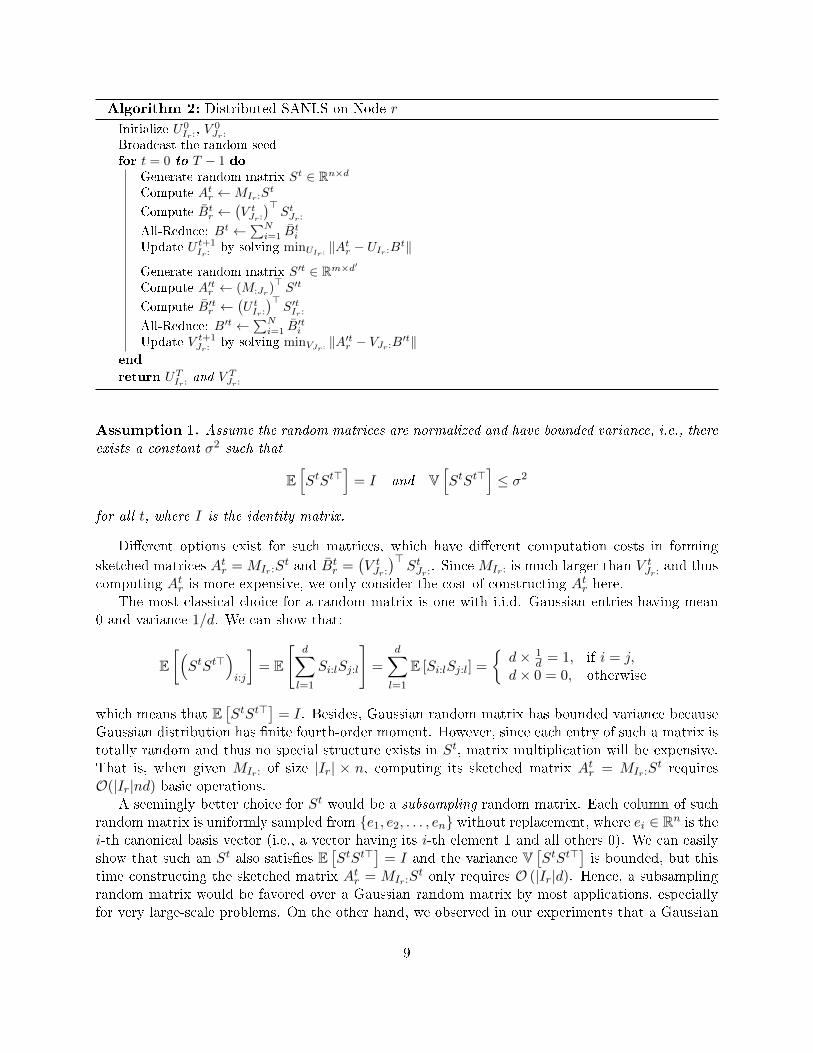
Algorithm 2: Distributed SANLS on Node r

Initialize U0Ir:, V 0

Jr:

Broadcast the random seedfor t = 0 to T − 1 do

Generate random matrix St ∈ Rn×d

Compute Atr ←MIr:S

t

Compute B̄tr ←

(V tJr:

)>StJr:

All-Reduce: Bt ←∑N

i=1 B̄ti

Update U t+1Ir:

by solving minUIr :‖At

r − UIr:Bt‖

Generate random matrix S′t ∈ Rm×d′

Compute A′tr ← (M:Jr)>S′t

Compute B̄′tr ←(U tIr:

)>S′tIr:

All-Reduce: B′t ←∑N

i=1 B̄′ti

Update V t+1Jr:

by solving minVJr :‖A′tr − VJr:B

′t‖end

return UTIr:

and V TJr:

Assumption 1. Assume the random matrices are normalized and have bounded variance, i.e., there

exists a constant σ2 such that

E[StSt>

]= I and V

[StSt>

]≤ σ2

for all t, where I is the identity matrix.

Di�erent options exist for such matrices, which have di�erent computation costs in forming

sketched matrices Atr = MIr:S

t and B̄tr =

(V tJr:

)>StJr:. SinceMIr: is much larger than V t

Jr:and thus

computing Atr is more expensive, we only consider the cost of constructing At

r here.The most classical choice for a random matrix is one with i.i.d. Gaussian entries having mean

0 and variance 1/d. We can show that:

E[(StSt>

)i:j

]= E

[d∑

l=1

Si:lSj:l

]=

d∑l=1

E [Si:lSj:l] =

{d× 1

d = 1, if i = j,d× 0 = 0, otherwise

which means that E[StSt>] = I. Besides, Gaussian random matrix has bounded variance because

Gaussian distribution has �nite fourth-order moment. However, since each entry of such a matrix istotally random and thus no special structure exists in St, matrix multiplication will be expensive.That is, when given MIr: of size |Ir| × n, computing its sketched matrix At

r = MIr:St requires

O(|Ir|nd) basic operations.A seemingly better choice for St would be a subsampling random matrix. Each column of such

random matrix is uniformly sampled from {e1, e2, . . . , en} without replacement, where ei ∈ Rn is thei-th canonical basis vector (i.e., a vector having its i-th element 1 and all others 0). We can easilyshow that such an St also satis�es E

[StSt>] = I and the variance V

[StSt>] is bounded, but this

time constructing the sketched matrix Atr = MIr:S

t only requires O (|Ir|d). Hence, a subsamplingrandom matrix would be favored over a Gaussian random matrix by most applications, especiallyfor very large-scale problems. On the other hand, we observed in our experiments that a Gaussian

9

random matrix can result in a faster per-iteration convergence rate, because each column of thesketched matrix At

r contains entries from multiple columns of the original matrix and thus is moreinformative. Hence, it would be better to use a Gaussian matrix when the sketch size d is small andthus a O(|Ir|nd) complexity is acceptable, or when the network speed of the cluster is poor, hencewe should trade more local computation cost for less communication cost.

Although we only test two representative types of random matrices (i.e., Gaussian and subsam-pling random matrices), our framework is readily applicable for other choices, such as subsampledrandomized Hadamard transform (SRHT) [1, 28] and count sketch [3, 5, 35]. The choice of randommatrices is not the focus of this paper and left for future investigation.

3.6 Solving Subproblems

Before describing how to solve subproblem (11), let us make an important observation. As discussedin Section 2.4, the sketching technique has been applied in solving linear systems before. For a linearsystem, it is usually assumed that there exists a solution x∗ such that Ax∗ = b exactly holds. Hence,x∗ is also the solution to the sketched problem, namely, (SA)x∗ = Sb. However, the situation isdi�erent in matrix factorization. Note that for the distributed matrix factorization problem weusually have

minUIr :∈R

|Ir |×k+

∥∥∥MIr: − UIr:Vt>∥∥∥2F6= 0.

So, for the sketched subproblem (11), which can be equivalently written as

minUIr :∈R

|Ir |×k+

∥∥∥(MIr: − UIr:Vt>)St∥∥∥2F,

the non-zero entries of the residual matrix(MIr: − UIr:V

t>) will be scaled by the matrix St atdi�erent levels. As a consequence, the optimal solution will be shifted because of sketching. Thisfact alerts us that for SANLS, we need to update U t+1 by exploiting the sketched subproblem (11)to step towards the true optimal solution and avoid convergence to the solution of the sketchedsubproblem.

3.6.1 Projected Gradient Descent

A natural method is to use one step of projected gradient descent for the sketched subproblem:

U t+1Ir:

= max

{U tIr: − ηt ∇UIr :

∥∥Atr − UIr:B

t∥∥2F

∣∣∣UIr :=Ut

Ir :

, 0

}= max

{U tIr: − 2ηt

[U tIr:B

tBt> −AtrB

t>], 0}, (12)

where ηt > 0 is the step size and max{·, ·} denotes the entry-wise maximum operation.To exploit the nature of this algorithm, we further expand the gradient:

∇UIr :

∥∥Atr − UIr:B

t∥∥2F

= 2[UIr:B

tBt> −AtrB

t>]

(10)= 2

[UIr:

(V t>St

)(V t>St

)>−(MIr:S

t) (V t>St

)>]=2[UIr:V

t>(StSt>

)V t −MIr:

(StSt>

)V t].

10

By taking the expectation of the above equation, and using the fact E[StSt>] = I, we have:

E[∇UIr :

∥∥Atr − UIr:B

t∥∥2F

]= 2

[UIr:V

t>V t −MIr:Vt]

= ∇UIr :

∥∥∥MIr: − UIr:Vt>∥∥∥2F,

which means that the gradient of the sketched subproblem is equivalent to the gradient of theoriginal problem on expectation4. Therefore, such a step of gradient descent can be interpreted asa (generalized) stochastic gradient descent (SGD) [32] method on the original subproblem. Thus,according to the theory of SGD, we naturally require the step sizes {ηt} to be diminishing, i.e.,ηt → 0 as t increases.

In the gradient descent step (12), the computational cost mainly comes from two matrix mul-tiplications: BtBt> and At,rB

t>. Note that Atr and B

t are of sizes |Ir| × d and k × d respectively,thus the gradient descent step takes O (kd(|Ir|+ k)) in total.

3.6.2 Regularized Coordinate Descent

However, it is well known that the gradient descent method converges slowly when solving NMFsubproblems, while the coordinate descent method, namely the HALS method for NMF, is quitee�cient [8]. Still, because of its very fast convergence, HALS should not be applied to the sketchedsubproblem, since it converges to the optimal solution of the subproblem after just a few iterations.As we have discussed in the beginning of Section 3.6, this is undesirable because it shifts the solutionaway from the true optimal solution. Therefore, we need to develop a method which resembles HALSbut will not converge towards the solutions of the sketched subproblems.

To achieve this, we add a regularization term to the sketched subproblem (11). The new sub-problem is:

minUIr :∈R

|Ir |×k+

∥∥Atr − UIr:B

t∥∥2F

+ µt∥∥UIr: − U t

Ir:

∥∥2F, (13)

where µt > 0 is a parameter. This regularization is reminiscent to the proximal point method [40]in optimization. Although the objective function is changed, the real e�ect of the regularizationterm is to control the step size, and thus it does not change the solution to which the algorithmultimately converges. Therefore, parameter µt plays a role similar to 1/ηt in projected gradientdescent; we require µt → +∞ to enforce the convergence of the whole algorithm, e.g., µt = t.

To solve (13) e�ciently, we apply coordinate descent. At each step, only one column of UIr:,say UIr,j where j ∈ {1, 2, . . . , k}, is updated:

minUIr :j∈R

|Ir |+

∥∥∥∥Atr − UIr:jB

tj: −

∑l 6=j

UIr:lBtl:

∥∥∥∥2F

+ µt∥∥UIr:j − U t

Ir:j

∥∥22.

It is not hard to see that the above problem is still row-independent, which means that each entryof the row vector UIr:j can be solved independently. For example, for any i ∈ Ir, the solution ofU t+1i:j is given by:

4We generalize such property as Lemma 2, shown in Appendix B.1.

11

U t+1i:j = arg min

Ui:j≥0

∥∥∥∥ (Atr

)i:− Ui:jB

tj: −

∑l 6=j

Ui:lBtl:

∥∥∥∥22

+ µt∥∥Ui:j − U t

i:j

∥∥22

= max

{µtU

ti:j +

(At

r

)i:Bt>

j: −∑

l 6=j Ui:lBtl:B

t>j:

Btj:B

t>j: + µt

, 0

}. (14)

At each step of coordinate descent, we choose the column j from {1, 2, . . . , k} successively.When updating column j at iteration t, the columns l < j have already been updated and thusUIr:l = U t+1

Ir:l, while the columns l > j are old so UIr:l = U t

Ir:l. Based on this, (14) can be equivalently

written in vector form as:

U t+1Ir:j

= max

{µtU

tIr:j

+AtrB

t>j: −

∑j−1l=1 B

tl:B

t>j: U

t+1Ir:l−∑k

l=j+1Btl:B

t>j: U

tIr:l

Btj:B

t>j: + µt

, 0

}.

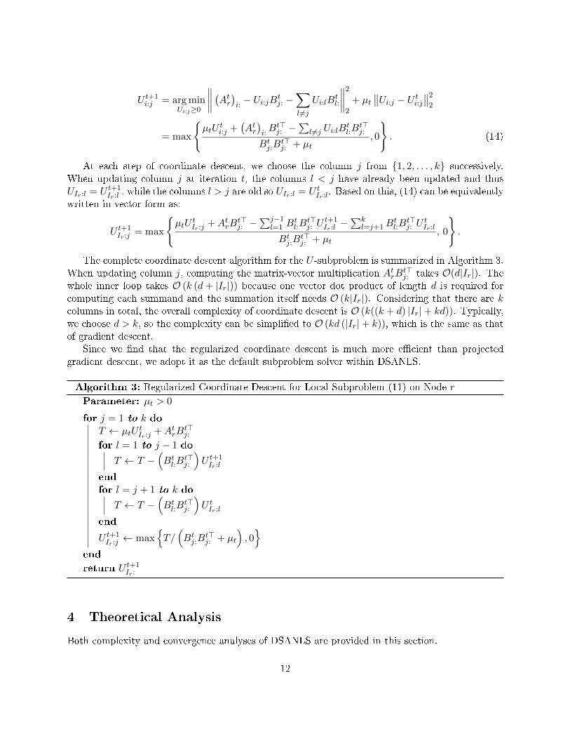
The complete coordinate descent algorithm for the U -subproblem is summarized in Algorithm 3.When updating column j, computing the matrix-vector multiplication At

rBt>j: takes O(d|Ir|). The

whole inner loop takes O (k (d+ |Ir|)) because one vector dot product of length d is required forcomputing each summand and the summation itself needs O (k|Ir|). Considering that there are kcolumns in total, the overall complexity of coordinate descent is O (k((k + d) |Ir|+ kd)). Typically,we choose d > k, so the complexity can be simpli�ed to O (kd (|Ir|+ k)), which is the same as thatof gradient descent.

Since we �nd that the regularized coordinate descent is much more e�cient than projectedgradient descent, we adopt it as the default subproblem solver within DSANLS.

Algorithm 3: Regularized Coordinate Descent for Local Subproblem (11) on Node r

Parameter: µt > 0

for j = 1 to k doT ← µtU

tIr:j

+AtrB

t>j:

for l = 1 to j − 1 do

T ← T −(Bt

l:Bt>j:

)U t+1Ir:l

end

for l = j + 1 to k do

T ← T −(Bt

l:Bt>j:

)U tIr:l

end

U t+1Ir:j← max

{T/(Bt

j:Bt>j: + µt

), 0}

end

return U t+1Ir:

4 Theoretical Analysis

Both complexity and convergence analyses of DSANLS are provided in this section.

12

4.1 Complexity Analysis

We now analyze the computational and communication costs of our DSANLS algorithm, when usingsubsampling random sketch matrices. The computational complexity at each node is:

O( generating St︷︸︸︷

d +

constructing Atr and Bt︷︸︸︷

|Ir|d +

solving subproblem︷ ︸︸ ︷kd(|Ir|+ k)

)= O (kd(|Ir|+ k)) ≈ O

(kd(mN

+ k))

(15)

Moreover, as we have shown in Section 3.4, the communication cost of DSANLS is O (kd).On the other hand, for a classical implementation of distributed HALS [7], the computational

cost is

O (kn (|Ir|+ k)) ≈ O(kn(mN

+ k))

(16)

and the communication cost is O (kn) due to the all-gathering of V t's.Comparing the above quantities, we observe an n/d� 1 speedup of our DSANLS algorithm over

HALS in both computation and communication. However, we empirically observed that DSANLShas a slower per-iteration convergence rate (i.e., it needs more iterations to converge). Still, aswe will show in the next section, in practice, DSANLS is superior to alternative distributed NMFalgorithms, after taking all factors into account.

4.2 Convergence Analysis

Here we provide theoretical convergence guarantees for the proposed SANLS and DSANLS algo-rithms. We show that SANLS and DSANLS converge to a stationary point.

4.2.1 Assumptions

To establish convergence result, Assumption 2 is needed �rst.

Assumption 2. Assume all the iterates U t and V t have uniformly bounded norms, which means

that there exists a constant R such that

‖U t‖F ≤ R and ‖V t‖F ≤ R

for all t.

We experimentally observed that this assumption holds in practice, as long as the step sizes usedare not too large. Besides, Assumption 2 can also be enforced by imposing additional constraints,e.g.:

Ui:l ≤√

2‖M‖F and Vj:l ≤√

2‖M‖F ∀i, j, l, (17)

with which we have R = max{m,n}k√

2‖M‖F . Such constraints can be very easily handled byboth of our projected gradient descent and regularized coordinate descent solvers. Lemma 1 showsthat imposing such extra constraints does not prevent us from �nding the global optimal solution.The lemma is proved in Appendix A.

Lemma 1. If the optimal solution to the original problem (1) exists, there is at least one global

optimal solution in the domain (17).

13

4.2.2 Convergence Theorem

Based on Assumptions 1 (see Section 3.5) and 2, we now can formally show our main convergenceresult:

Theorem 1. Under Assumptions 1 and 2, if the step sizes satisfy

∞∑t=1

ηt =∞ and

∞∑t=1

η2t <∞,

for projected gradient descent, or

∞∑t=1

1/µt =∞ and

∞∑t=1

1/µ2t <∞,

for regularized coordinate descent, then SANLS and DSANLS with either sub-problem solver will

converge to a stationary point of problem (1) with probability 1.

Here stationary point means a point whose projected gradient is zero. In convex optimizationproblems, stationary points must be globally optimal solutions. Although our problem is non-convexand hence its stationary points do not necessarily correspond to global optima, considering that itis NP-hard to �nd a global optimal solution for a general non-convex problems, convergence to astationary point is already the best theoretical result that one can hope for. The proof of Theorem1 can be found in Appendix B.

5 Experimental Evaluation

This section includes an experimental evaluation of our algorithm on both dense and sparse realdata matrices.

5.1 Datasets

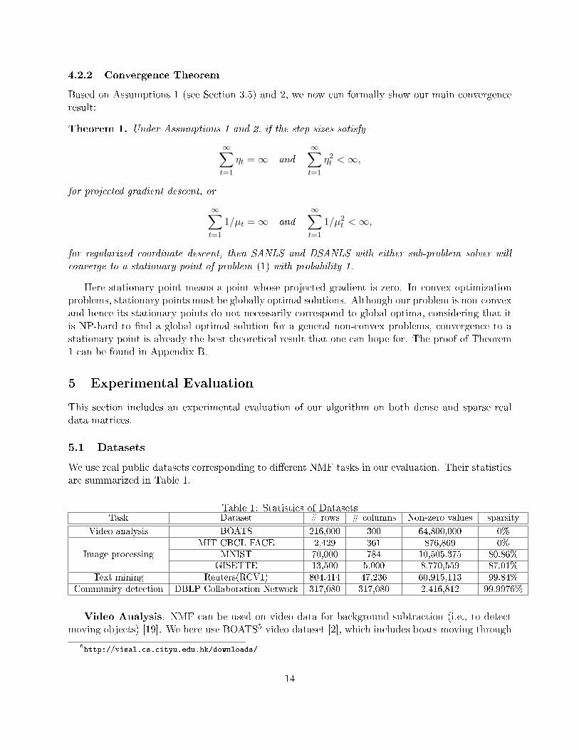
We use real public datasets corresponding to di�erent NMF tasks in our evaluation. Their statisticsare summarized in Table 1.

Table 1: Statistics of DatasetsTask Dataset # rows # columns Non-zero values sparsity

Video analysis BOATS 216,000 300 64,800,000 0%

Image processingMIT CBCL FACE 2,429 361 876,869 0%

MNIST 70,000 784 10,505,375 80.86%GISETTE 13,500 5,000 8,770,559 87.01%

Text mining Reuters(RCV1) 804,414 47,236 60,915,113 99.84%

Community detection DBLP Collaboration Network 317,080 317,080 2,416,812 99.9976%

Video Analysis. NMF can be used on video data for background subtraction (i.e., to detectmoving objects) [19]. We here use BOATS5 video dataset [2], which includes boats moving through

5http://visal.cs.cityu.edu.hk/downloads/

14

water. The video has 15 fps and it is saved as a sequence of png �les, whose format is RGB with aframe size of 360×200. We use `Boats2' which contains one boat close to the camera for 300 framesand reshape the matrix such that every RGB frame is a column of our matrix; the �nal matrix isdense with size 216, 000× 300.

Image Processing. The �rst dataset we use for this application is MIT CBCL FACE DATABASE6

as in [22]. To form the vectorized matrix, whose size is 2429 × 361, we use all 2,429 face images(each with 19 × 19 pixels) in the original training set. The second dataset is MINST7, which is awidely used handwritten digits dataset. We use all 70,000 samples including both training and testset, and form the vectorized matrix. The third dataset is GISETTE8, from another handwrittendigit recognition problem. This dataset is one of the �ve datasets used in the NIPS 2003 featureselection challenge. We use all pictures in the training, validation, and test datasets and form thevectorized matrix, whose size is 5, 000× 13, 500.

Text Mining. We use the Reuters document corpora9 as in [44]. Reuters Corpus Volume I(RCV1) [24] is an archive of over 800,000 manually categorized newswire stories made available byReuters, Ltd. for research purposes. It has 804,414 samples and 47,236 features. Non-zero valuescontain cosine-normalized, log TF-IDF vectors. A nearly chronological split is also utilized, whichfollows the o�cial LYRL2004 chronological split.

Community Detection. We use the DBLP collaboration network10. It is a co-authorshipgraph where two authors are connected if they have published at least one paper together. Weconvert it to an adjacency matrix, which has 2,416,812 non-zero values, taking 0.0024% of thewhole matrix.

5.2 Setup

We conduct our experiments on the Linux cluster of our institute with a total of 96 nodes. Eachnode contains 8-core Intel(R) Core(TM) i7-3770 CPU @ 1.60GHz cores and 16 GB of memory. Ouralgorithm is implemented in C using the Intel Math Kernel Library (MKL) and Message PassingInterface (MPI). We use 10 nodes by default. Since tuning the factorization rank k is outside thescope of this paper, we use 100 as default value of k. Because of the large sizes of RCV1 and DBLP,we only use subsampling random matrices for them, as the use of Gaussian random matrices is tooslow.

We evaluate DSANLS with subsampling and Gaussian random matrices, denoted by DSANLS/Sand DSANLS/G, respectively, using regularized coordinate descent as the default subproblem solver.As mentioned in [16, 17], it is unfair to compare with a Hadoop implementation, as Hadoop is notdesigned for high performance computing of iterative numerical algorithms. Although Spark is moreappropriate than Hadoop for iterative algorithms, [9] further shows that Spark implementationsincur signi�cant overheads due to task scheduling, task start delays, and idle time caused by Sparkstragglers, and it is usually around 4x slower compared to MPI implementations. Therefore, we onlycompare DSANLS with MPI-FAUN11 (all MPI-FAUN-MU, MPI-FAUN-HALS, and MPI-FAUN-

6http://cbcl.mit.edu/software-datasets/FaceData2.html7http://yann.lecun.com/exdb/mnist/8http://clopinet.com/isabelle/Projects/NIPS2003/#challenge9we use the second version RCV1-v2, which can be found in http://jmlr.csail.mit.edu/papers/volume5/

lewis04a/10http://snap.stanford.edu/data/com-DBLP.html11public code available at https://github.com/ramkikannan/nmflibrary

15

0 10 20 30 40Time (s)

0.0

0.2

0.4

0.6

0.8

1.0Re

lativ

e Er

ror

DSANLS/SDSANLS/GMUHALSANLS/BPP

(a) BOATS

0.0 0.2 0.4 0.6 0.8 1.0 1.2 1.4Time (s)

0.0

0.2

0.4

0.6

0.8

1.0

Rela

tive

Erro

r

DSANLS/SDSANLS/GMUHALSANLS/BPP

(b) FACE

0.0 2.5 5.0 7.5 10.0 12.5 15.0 17.5Time (s)

0.0

0.2

0.4

0.6

0.8

1.0

Rela

tive

Erro

r

DSANLS/SDSANLS/GMUHALSANLS/BPP

(c) MNIST

0 1 2 3 4 5 6 7 8Time (s)

0.5

0.6

0.7

0.8

0.9

1.0

Rela

tive

Erro

r

DSANLS/SDSANLS/GMUHALSANLS/BPP

(d) GISETTE

0 100 200 300 400 500Time (s)

0.80

0.85

0.90

0.95

1.00

1.05

Rela

tive

Erro

r

SANLS/SMUHALSANLS/BPP

(e) RCV1

0 10 20 30 40 50 60 70 80Time (s)

0.94

0.96

0.98

1.00

1.02

1.04

Rela

tive

Erro

r

SANLS/SMUHALSANLS/BPP

(f) DBLP

Figure 2: Relative error over time

ABPP implementations), which is the �rst and the state-of-the-art C++/MPI implementation withMKL and Armadillo. For parameters pc and pr in MPI-FAUN, we use the optimal values for eachdataset, according to the recommendations in [16, 17].

16

5 10 15Node number

50

100

150

2001/

time

(s1 )

DSANLS/SDSANLS/GMUHALSANLS/BPP

(a) FACE

5 10 15Node number

0

5

10

15

20

1/tim

e (s

1 )

DSANLS/SDSANLS/GMUHALSANLS/BPP

(b) MNIST

5 10 15Node number

0.00

0.05

0.10

0.15

0.20

0.25

1/tim

e (s

1 )

DSANLS/SMUHALSANLS/BPP

(c) RCV1

5 10 15Node number

0.0

0.2

0.4

0.6

0.8

1.0

1/tim

e (s

1 ) DSANLS/SMUHALSANLS/BPP

(d) DBLP

Figure 3: Reciprocal of per-iteration time as a function of cluster size

5.3 Results

5.3.1 Performance Comparison

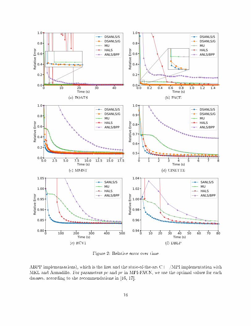
We use the relative error of the low rank approximation compared to the original matrix to measurethe e�ectiveness of NMF by DSANLS with MPI-FAUN. This error measure was been widely usedin previous work [16, 17, 19] and is formally de�ned as∥∥∥M − UV >∥∥∥

F/ ‖M‖F .

Since the time for each iteration is signi�cantly reduced by our proposed DSANLS compared toMPI-FAUN, in Figure 2, we show the relative error over time for DSANLS and MPI-FAUN imple-mentations of MU, HALS, and ANLS/BPP on the 6 real public datasets. Observe that DSANLS/Sperforms best in all 6 datasets, although DSANLS/G has faster per-iteration convergence rate. MUconverges relatively slowly and usually has a bad convergence result; on the other hand HALS mayoscillate in the early rounds12, but converges quite fast and to a good solution. Surprisingly, al-

12HALS does not guarantee the objective function to decrease monotonically.

17

0 20 40 60 80 100Time (s)

0.90

0.92

0.94

0.96

0.98

1.00Re

lativ

e Er

ror

DSANLS/SMUHALSANLS/BPP

(a) k=20

0 50 100 150 200 250Time (s)

0.875

0.900

0.925

0.950

0.975

1.000

Rela

tive

Erro

r

DSANLS/SMUHALSANLS/BPP

(b) k=50

0 250 500 750 1000 1250 1500Time (s)

0.75

0.80

0.85

0.90

0.95

1.00

Rela

tive

Erro

r

DSANLS/SMUHALSANLS/BPP

(c) k=200

0 1000 2000 3000 4000Time (s)

0.7

0.8

0.9

1.0

Rela

tive

Erro

r

DSANLS/SMUHALSANLS/BPP

(d) k=500

Figure 4: Relative error over time, varying k value

though ANLS/BPP is considered to be the state-of-art NMF algorithm, it does not perform well inall 6 datasets. As we will see, this is due to its high per-iteration cost.

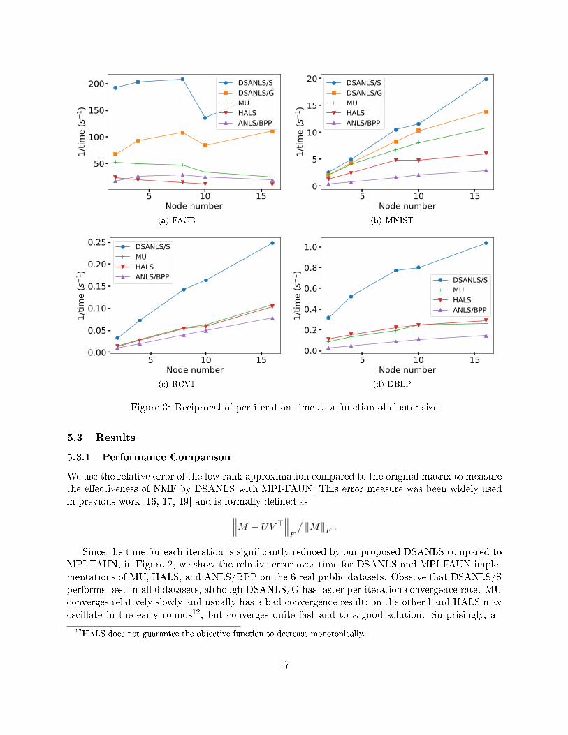
5.3.2 Scalability Comparison

We vary the number of nodes used in the cluster from 2 to 16 and record the average time for 100iterations of each algorithm. Figure 3 shows the reciprocal of per-iteration time as a function ofthe number of nodes used. All algorithms exhibit good scalability for all datasets (nearly a straightline), except for FACE (i.e., Figure 3(a)). FACE is the smallest dataset, whose number of columns is300, while k is set to 100 by default. When n/N is smaller than k, the complexity is dominated by k,hence, increasing the number of nodes does not reduce the computational cost, but may increase thecommunication overhead. In general, we can observe that DSANLS/Subsampling has the lowestper-iteration cost compared to all other algorithms, and DSANLS/Gaussian has similar cost toMU and HALS. ANLS/BPP has the highest per-iteration cost, explaining the bad performance ofANLS/BPP in Figure 2.

18

0 20 40 60 80 100Iteration

0.0

0.1

0.2

0.3

0.4

0.5Re

lativ

e Er

ror

DSANLS-RCD/SDSANLS-RCD/GDSANLS-PGD/SDSANLS-PGD/G

(a) BOATS

0 20 40 60 80 100Iteration

0.00

0.02

0.04

0.06

0.08

0.10

Rela

tive

Erro

r

DSANLS-RCD/SDSANLS-RCD/GDSANLS-PGD/SDSANLS-PGD/G

(b) FACE

0 20 40 60 80 100Iteration

0.4

0.5

0.6

0.7

0.8

0.9

1.0

Rela

tive

Erro

r

DSANLS-RCD/SDSANLS-RCD/GDSANLS-PGD/SDSANLS-PGD/G

(c) GISETTE

0 20 40 60 80 100Iteration

0.80

0.85

0.90

0.95

1.00

1.05

Rela

tive

Erro

r

DSANLS-RCD/SDSANLS-PGD/S

(d) RCV1

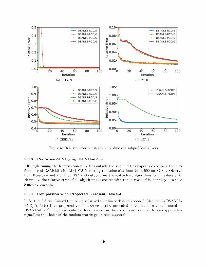
Figure 5: Relative error per-iteration of di�erent subproblem solvers

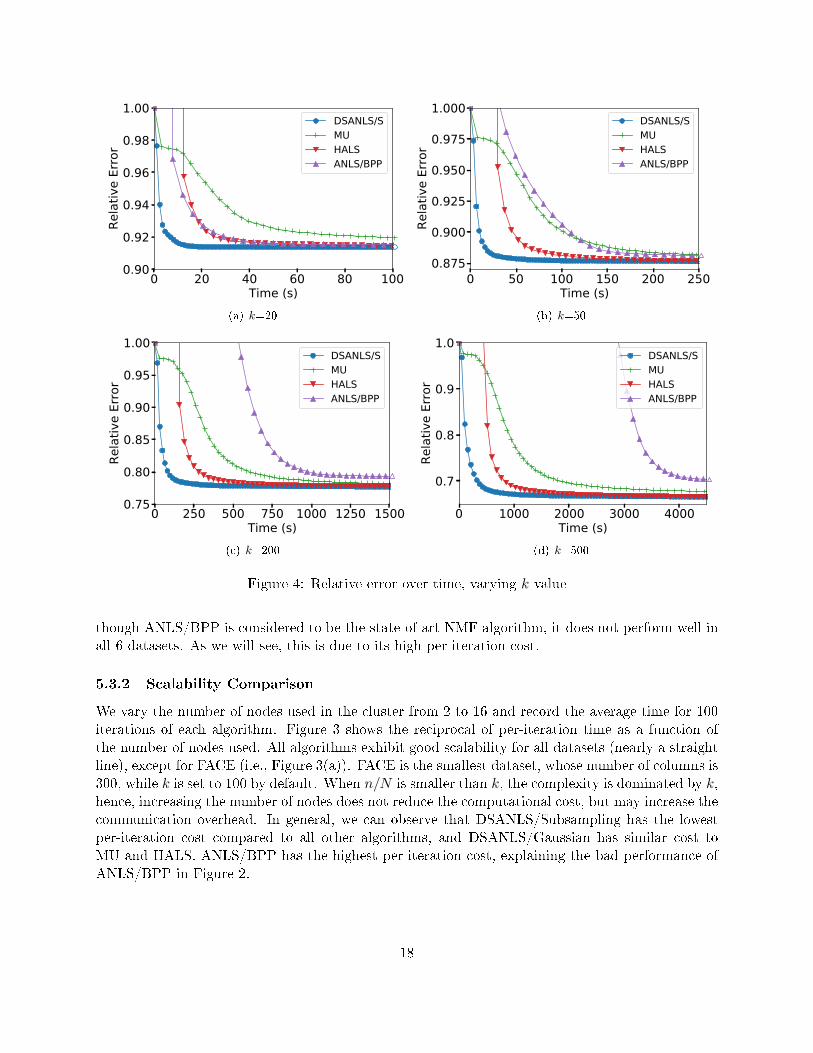
5.3.3 Performance Varying the Value of k

Although tuning the factorization rank k is outside the scope of this paper, we compare the per-formance of DSANLS with MPI-FAUN varying the value of k from 20 to 500 on RCV1. Observefrom Figures 4 and 2(e) that DSANLS outperforms the state-of-art algorithms for all values of k.Naturally, the relative error of all algorithms decreases with the increase of k, but they also takelonger to converge.

5.3.4 Comparison with Projected Gradient Descent

In Section 3.6, we claimed that our regularized coordinate descent approach (denoted as DSANLS-RCD) is faster than projected gradient descent (also presented in the same section, denoted asDSANLS-PGD). Figure 5 con�rms the di�erence in the convergence rate of the two approachesregardless the choice of the random matrix generation approach.

19

6 Conclusion

In this paper, we presented a novel distributed NMF algorithm that can be used for scalable analyticsof high dimensional matrix data. Our approach follows the general framework of ANLS, but utilizesmatrix sketching to reduce the problem size of each NLS subproblem. We discussed and comparedtwo di�erent approaches for generating random matrices (i.e. Gaussian and subsampling randommatrices). Then, we presented two subproblem solvers for our general framework, and theoreticallyproved their convergence. We analyzed the per-iteration computational and communication cost ofour approach and its convergence, showing its superiority compared to the previous state-of-the-art. Our experiments on several real datasets show that our method converges fast to an accuratesolution and scales well with the number of cluster nodes used. In the future, we plan to study theapplication of DSANLS to dense or sparse tensors.

References

[1] N. Ailon and B. Chazelle. Approximate nearest neighbors and the fast johnson-lindenstrausstransform. In STOC, pages 557�563. ACM, 2006.

[2] A. B. Chan, V. Mahadevan, and N. Vasconcelos. Generalized stau�er�grimson backgroundsubtraction for dynamic scenes. Machine Vision and Applications, 22(5):751�766, 2011.

[3] M. Charikar, K. Chen, and M. Farach-Colton. Finding frequent items in data streams. Theo-retical Computer Science, 312(1):3�15, 2004.

[4] A. Cichocki and P. Anh-Huy. Fast local algorithms for large scale nonnegative matrix andtensor factorizations. IEICE transactions on fundamentals of electronics, communications and

computer sciences, 92(3):708�721, 2009.

[5] K. L. Clarkson and D. P. Woodru�. Low rank approximation and regression in input sparsitytime. In STOC, pages 81�90. ACM, 2013.

[6] M. E. Daube-Witherspoon and G. Muehllehner. An iterative image space reconstruction algo-rthm suitable for volume ect. IEEE transactions on medical imaging, 5(2):61�66, 1986.

[7] J. P. Fairbanks, R. Kannan, H. Park, and D. A. Bader. Behavioral clusters in dynamic graphs.Parallel Computing, 47:38�50, 2015.

[8] N. Gillis. The why and how of nonnegative matrix factorization. Regularization, Optimization,Kernels, and Support Vector Machines, 12(257), 2014.

[9] A. Gittens, A. Devarakonda, E. Racah, M. Ringenburg, L. Gerhardt, J. Kottalam, J. Liu,K. Maschho�, S. Canon, J. Chhugani, et al. Matrix factorization at scale: a comparisonof scienti�c data analytics in spark and c+ mpi using three case studies. arXiv preprint

arXiv:1607.01335, 2016.

[10] R. M. Gower and P. Richtárik. Randomized iterative methods for linear systems. SIAM Journal

on Matrix Analysis and Applications, 36(4):1660�1690, 2015.

20

[11] L. Grippo and M. Sciandrone. On the convergence of the block nonlinear gauss�seidel methodunder convex constraints. Operations research letters, 26(3):127�136, 2000.

[12] D. Grove, J. Milthorpe, and O. Tardieu. Supporting array programming in x10. In ARRAY,page 38. ACM, 2014.

[13] N. Guan, D. Tao, Z. Luo, and B. Yuan. Nenmf: an optimal gradient method for nonnegativematrix factorization. IEEE Transactions on Signal Processing, 60(6):2882�2898, 2012.

[14] K. Huang, N. D. Sidiropoulos, and A. Swami. Non-negative matrix factorization revisited:Uniqueness and algorithm for symmetric decomposition. IEEE Transactions on Signal Pro-

cessing, 62(1):211�224, 2014.

[15] K. Kanjani. Parallel non negative matrix factorization for document clustering. CPSC-659

(Parallel and Distributed Numerical Algorithms) course. Texas A&M University, Tech. Rep,2007.

[16] R. Kannan, G. Ballard, and H. Park. A high-performance parallel algorithm for nonnegativematrix factorization. In PPoPP, page 9. ACM, 2016.

[17] R. Kannan, G. Ballard, and H. Park. Mpi-faun: An mpi-based framework for alternating-updating nonnegative matrix factorization. arXiv preprint arXiv:1609.09154, 2016.

[18] H. Kim and H. Park. Nonnegative matrix factorization based on alternating nonnegativity con-strained least squares and active set method. SIAM journal on matrix analysis and applications,30(2):713�730, 2008.

[19] J. Kim, Y. He, and H. Park. Algorithms for nonnegative matrix and tensor factorizations: Auni�ed view based on block coordinate descent framework. Journal of Global Optimization,58(2):285�319, 2014.

[20] J. Kim and H. Park. Fast nonnegative matrix factorization: An active-set-like method andcomparisons. SIAM Journal on Scienti�c Computing, 33(6):3261�3281, 2011.

[21] I. Kotsia, S. Zafeiriou, and I. Pitas. A novel discriminant non-negative matrix factorizationalgorithm with applications to facial image characterization problems. IEEE Transactions on

Information Forensics and Security, 2(3):588�595, 2007.

[22] D. D. Lee and H. S. Seung. Learning the parts of objects by non-negative matrix factorization.Nature, 401(6755):788�791, 1999.

[23] D. D. Lee and H. S. Seung. Algorithms for non-negative matrix factorization. In NIPS, pages556�562, 2001.

[24] D. D. Lewis, Y. Yang, T. G. Rose, and F. Li. Rcv1: A new benchmark collection for textcategorization research. JMLR, 5(Apr):361�397, 2004.

[25] R. Liao, Y. Zhang, J. Guan, and S. Zhou. Cloudnmf: a mapreduce implementation of nonneg-ative matrix factorization for large-scale biological datasets. Genomics, proteomics & bioinfor-

matics, 12(1):48�51, 2014.

21

[26] C.-J. Lin. Projected gradient methods for nonnegative matrix factorization. Neural computa-tion, 19(10):2756�2779, 2007.

[27] C. Liu, H.-c. Yang, J. Fan, L.-W. He, and Y.-M. Wang. Distributed nonnegative matrixfactorization for web-scale dyadic data analysis on mapreduce. In WWW, pages 681�690.ACM, 2010.

[28] Y. Lu, P. Dhillon, D. P. Foster, and L. Ungar. Faster ridge regression via the subsampledrandomized hadamard transform. In NIPS, pages 369�377, 2013.

[29] J. Mairal. Stochastic majorization-minimization algorithms for large-scale optimization. InNIPS, pages 2283�2291, 2013.

[30] E. Mejía-Roa, D. Tabas-Madrid, J. Setoain, C. García, F. Tirado, and A. Pascual-Montano.Nmf-mgpu: non-negative matrix factorization on multi-gpu systems. BMC bioinformatics,16(1):1, 2015.

[31] X. Meng, J. Bradley, B. Yuvaz, E. Sparks, S. Venkataraman, D. Liu, J. Freeman, D. Tsai,M. Amde, S. Owen, et al. Mllib: Machine learning in apache spark. JMLR, 17(34):1�7, 2016.

[32] A. Nemirovski, A. Juditsky, G. Lan, and A. Shapiro. Robust stochastic approximation approachto stochastic programming. SIAM Journal on optimization, 19(4):1574�1609, 2009.

[33] J. Neveu. Discrete-parameter martingales, volume 10. Elsevier, 1975.

[34] V. P. Pauca, F. Shahnaz, M. W. Berry, and R. J. Plemmons. Text mining using non-negativematrix factorizations. In SDM, pages 452�456. SIAM, 2004.

[35] N. Pham and R. Pagh. Fast and scalable polynomial kernels via explicit feature maps. In ACM

SIGKDD, pages 239�247. ACM, 2013.

[36] M. Pilanci and M. J. Wainwright. Iterative hessian sketch: Fast and accurate solution approx-imation for constrained least-squares. JMLR, pages 1�33, 2015.

[37] M. Pilanci and M. J. Wainwright. Newton sketch: A linear-time optimization algorithm withlinear-quadratic convergence. arXiv preprint arXiv:1505.02250, 2015.

[38] I. Psorakis, S. Roberts, M. Ebden, and B. Sheldon. Overlapping community detection usingbayesian non-negative matrix factorization. Physical Review E, 83(6):066114, 2011.

[39] S. A. Robila and L. G. Maciak. A parallel unmixing algorithm for hyperspectral images. InOptics East, pages 63840F�63840F. International Society for Optics and Photonics, 2006.

[40] R. T. Rockafellar. Monotone operators and the proximal point algorithm. SIAM journal on

control and optimization, 14(5):877�898, 1976.

[41] S. A. Vavasis. On the complexity of nonnegative matrix factorization. SIAM Journal on

Optimization, 20(3):1364�1377, 2009.

[42] F. Wang and P. Li. E�cient nonnegative matrix factorization with random projections. InSDM, pages 281�292. SIAM, 2010.

22

[43] Y.-X. Wang and Y.-J. Zhang. Nonnegative matrix factorization: A comprehensive review.TKDE, 25(6):1336�1353, 2013.

[44] W. Xu, X. Liu, and Y. Gong. Document clustering based on non-negative matrix factorization.In SIGIR, pages 267�273. ACM, 2003.

[45] J. Yin, L. Gao, and Z. M. Zhang. Scalable nonnegative matrix factorization with block-wiseupdates. In ECML-PKDD, pages 337�352. Springer, 2014.

[46] R. Zdunek and A. Cichocki. Non-negative matrix factorization with quasi-newton optimization.In ICAISC, pages 870�879. Springer, 2006.

A Proof of Lemma 1

Proof of Lemma 1. Suppose (U∗, V ∗) is the global optimal solution but fails to satisfy (17). If thereexist indices i, j, l such that U∗i:l · V ∗j:l > 2‖M‖F , then∥∥∥M − U∗V ∗>∥∥∥2

F≥(U∗i:l · V ∗j:l −Mi:j

)2> (2‖M‖F − ‖M‖F )2 ≥ ‖M‖2F .

However, simply choosing U = 0 and V = 0 will yield a smaller error ‖M‖2F , which contradicts thefact that (U∗, V ∗) is optimal. Therefore, if we de�ne αl = maxi U

∗i:l and βl = maxj V

∗j:l, we must

have αl · βl ≤ 2‖M‖F for each l. Now we construct a new solution (U, V ) by:

U i:l = U∗i:l ·√βl/αl and V j:l = V ∗j:l ·

√αl/βl.

Note that

U i:l ≤ αl ·√βl/αl =

√αl · βl ≤

√2‖M‖F ,

V j:l ≤ βl ·√αl/βl =

√αl · βl ≤

√2‖M‖F ,

so (U, V ) satisfy (17). Besides,∥∥∥M − U V >∥∥∥2F

=∑i,j

(Mi:j −

∑l

U i:lV j:l

)2=∑i,j

(Mi:j −

∑l

U∗i:l ·√βl/αl · V ∗j:l ·

√αl/βl

)2=∑i,j

(Mi:j −

∑l

U∗i:l · V ∗j:l)2

= ‖M − U∗V ∗>‖2F ,

which means that (U, V ) is also an optimal solution. In short, for any optimal solution of (1) outsidethe domain (17), there exists a corresponding global optimal solution satisfying (17), which furthermeans that there exists at least one optimal solution in the domain (17).

23

B Proof of the Main Theorem

For simplicity, we denote f(U, V ) = ‖M − UV >‖2F , f̃S = ‖MS − U(V >S)‖2F , and f̃ ′S′ = ‖M>S′ −V (U>S′)‖2F . Let Gt and G̃t denote the gradients of the above quantities, i.e.,

Gt , ∇U f(U, V t)∣∣U=Ut , G̃t , ∇U f̃St(U, V t)

∣∣∣U=Ut

,

G′t , ∇V f(U t+1, V )∣∣V=V t , G̃′t , ∇V f̃ ′S′t(U

t+1, V )∣∣∣V=V t

.

Besides, let

∆t ,1

ηt

(U t − U t+1

)and ∆′t ,

1

ηt

(V t − V t+1

).

B.1 Preliminary Lemmas

To prove Theorem 1, we need following lemmas (which are proved in Appendix B.3):

Lemma 2. Under Assumption 1 and 2, conditioned on U t and V t, G̃t and G̃′t are unbiased esti-

mators of Gt and G′t respectively with uniformly bounded variance.

Lemma 3. Assume X is a nonnegative random variable with mean µ and variance σ2, and c ≥ 0is a constant. Then we have

E [min{X, c}] ≥ min{c,µ

2

}·(

1− 4σ2

4σ2 + µ2

). (18)

Lemma 4. De�ne the function

φ(x, y, z) = min{|xy|, y2/2

}·(

1− 4z2

4z2 + y2

)≥ 0. (19)

Conditioned on U t and V t, there exists an uniform constant σ′2 > 0 such that

E[Gti:l ·∆t

i:l] ≥ φ(U ti:l/ηt, G

ti:l, σ

′2) (20)

and

E[G′tj:l ·∆′tj:l] ≥ φ(V tj:l/ηt, G

′tj:l, σ

′2)for any i, j, l.

Lemma 5 (Supermartingale Convergence Theorem, [33]). Let Yt, Zt and Wt, t = 0, 1, . . . , bethree sequences of random variables and let Ft, t = 0, 1, . . . , be sets of random variables such that

Ft ⊂ Ft+1. Suppose that

1. The random variables Yt, Zt andWt are nonnegative, and are functions of the random variables

in Ft.

2. For each t, we haveE[Yt+1|Ft] ≤ Yt − Zt +Wt.

3. There holds, with probability 1,∑∞

t=0Wt <∞.

24

Then we have∑∞

t=0 Zt < ∞, and the sequence Yt converges to a nonnegative random variable Y ,with probability 1.

Lemma 6 ([29]). For two nonnegative scalar sequences {at} and {bt}, if∑∞

t=0 ak = ∞ and∑∞t=0 atbt <∞, then

lim inft→∞

bt = 0.

Furthermore, if |bt+1 − bt| ≤ B · at for some constant B > 0, then

limt→∞

bt = 0.

B.2 Proof of Theorem 1

Proof of Theorem 1. Let us �rst focus on projected gradient descent. By conditioning on U t andV t, we have

f(U t+1, V t) =∥∥∥M − U t+1V t>

∥∥∥2F

=∥∥∥M − (U t − ηt∆t

)V t>

∥∥∥2F

=∥∥∥(M − U tV t>

)− ηt∆tV t>

∥∥∥2F

=∥∥∥M − U tV t>

∥∥∥2F− 2ηt

(M − U tV t>

)·(

∆tV t>)

+ η2t ‖∆tV t>‖2F

=f(U t, V t)− 2ηt

(M − U tV t>

)·(

∆tV t>)

+ η2t ‖∆tV t>‖2F . (21)

For the second term of (21), note that

2(M − U tV t>

)·(

∆tV t>)

= 2tr[(M − U tV t>

)V t∆t>

]= tr

[Gt∆t>

]=∑i,l

Gti:l ·∆t

i:l

By taking expectation and using Lemma 4, we obtain:

E[2(M − U tV t>

)·(

∆tV t>)]

=∑i,l

E[Gt

i:l ·∆ti:l

]≥∑i,l

φ(U ti:l/ηt, G

ti:l, σ

′2) .For simplicity, we will use the notation

Φ(U t/ηt, Gt) ,

∑i,l

φ(U ti:l/ηt, G

ti:l, σ

′2) .For the third term of (21), we can bound it in the following way:

‖∆tV t>‖2F ≤‖∆t‖2F · ‖V t‖2F ≤ ‖G̃t‖2F · ‖V t‖2F

=∥∥∥2(U tV t> −M)(StSt>)V t

∥∥∥2F· ‖V t‖2F

≤4‖M − U tV t>‖2F · ‖StSt>‖2F · ‖V t‖4F≤8(‖M‖2F + ‖U t‖2F · ‖V t‖2F

)· ‖StSt>‖2F · ‖V t‖4F

≤8(‖M‖2F +R4

)R4 · ‖StSt>‖2F ,

25

where in the last inequality we have applied Assumption 2. If we take expectation, we have

E‖∆tV t>‖2F ≤8(‖M‖2F +R4

)R4 · E‖StSt>‖2F

≤8(‖M‖2F +R4

)R4 ·

(∥∥∥E[StSt>]∥∥∥2 + V[StSt>]

)≤8(‖M‖2F +R4

)R4 ·

(n+ σ2

),

where mean-variance decomposition have been applied in the second inequality, and Assumption 1was used in the last line. For convenience, we will use

Γ , 8(‖M‖2F +R4

)R4 ·

(n+ σ2

)≥ 0

to denote this constant later on.By combining all results, we can rewrite (21) as

E[f(U t+1, V t)

]≤ f(U t, V t)− ηtΦ

(U t/ηt, G

t)

+ η2t Γ.

Likewise, conditioned on U t+1 and V t, we can prove a similar inequality for V :

E[f(U t+1, V t+1)

]≤ f(U t+1, V t)− ηtΦ

(V t/ηt, G

′t)+ η2t Γ′,

where Γ′ ≥ 0 is also some uniform constant. From de�nition, it is easy to see both Φ(U t/ηt, G

t)

and Φ(V t/ηt, G

′t) are nonnegative. Along with condition the condition∑∞

t=0 η2t <∞, we can apply

the Supermartingale Convergence Theorem (Lemma 5) with

Y2t = f(U t, V t), Y2t+1 = f(U t+1, V t),

Z2t = Φ(U t/ηt, G

t), Z2t+1 = Φ

(V t/ηt, G

′t) ,W2t = Γη2t , W2t+1 = Γ′η2t ,

and then conclude that both {f(U t+1, V t)} and {f(U t, V t)} will converge to a same value, andbesides:

∞∑t=0

ηt[Φ(U t/ηt, G

t)

+ Φ(V t/ηt, G

′t)] <∞,with probability 1. In addition, it is not hard to verify that

∣∣Φ (U t+1/ηt+1, Gt+1)− Φ

(U t/ηt, G

t)∣∣ ≤

C ·ηt for some constant C because of the boundness of the gradients. Then, by Lemma 6, we obtainthat

limt→∞

Φ(U t/ηt, G

t)

= limt→∞

∑i:l

φ(U ti:l/ηt, G

ti:l, σ

′2)→ 0.

Since each summand in the above is nonnegative, this equation further implies

limt→∞

φ(U ti:l/ηt, G

ti:l, σ

′2)→ 0

for all i and l. By looking into the de�nition of φ in (19), it is not hard to see that φ(U ti:l/ηt, G

ti:l, σ

′2)→0 if and only if min

{U ti:l/ηt,

∣∣Gti:l

∣∣}→ 0. Considering ηt > 0 and ηt → 0, we can conclude that

limt→∞

min{U ti:l,∣∣Gt

i:l

∣∣}→ 0

26

for all i, l, which means either the gradient Gti:l converges to 0, or U t

i:l converges to the boundary 0.In other words, the projected gradient at (U t, V t) w.r.t U converges to 0 as t → ∞. Likewise, wecan prove

limt→∞

min{V tj:l,∣∣G′tj:l∣∣}→ 0,

in a similar way, which completes the proof of projected gradient descent.The proof of regularized coordinate descent is similar to that of projected gradient descent, and

hence we only include a sketch proof here. The key here is to establish an inequality similar to(21), but with the di�erence that just one column rather than whole U or V is changed every time.Take U:1 as an example. An important observation is that when projection does not happen, wecan rewrite (14) as U t+1

:1 = U t:1 − G̃:1/(τt + Bt

j:Bt>j: ), which means that the moving direction of

regularized coordinate descent is the same as that of projected gradient descent, but with step sizebeing 1/(τt + Bt

j:Bt>j: ). Since both the expectation and variance of Bt

j:Bt>j: are bounded, we will

have 1/(τt + Btj:B

t>j: ) ≈ 1/τt when τt is large. Given these two reasons, we can out down a similar

inequality as (21). The remaining proof just follows the one for projected gradient descent.

B.3 Proof of Preliminary Lemmas

Proof of Lemma 2. Since the proof related to G̃′t is similar to G̃t, here we only focus on the latterone.

First, let us write down the de�nition of Gt and G̃t:

Gt = 2(U tV t> −M)V t and G̃t = 2(U tV t> −M)(StSt>)V t.

Therefore,

E[G̃t] =E[2(U tV t> −M)(StSt>)V t

]= 2(U tV t> −M)E[StSt>]V t

=2(U tV t> −M) I V t = 2(U tV t> −M)V t = Gt,

which means G̃t is an unbiased estimator of Gt. Besides, its variance is uniformly bounded because

V[G̃t] ≤V[2(U tV t> −M)i:(S

tSt>)V t:l

]≤4‖M − U tV t>‖2F · V[StSt>] · ‖V t‖2F≤8(‖M‖2F + ‖U t‖2F ‖V t‖2F

)· ‖V t‖2F · V[StSt>]

≤8(‖M‖2F +R4

)R2 · σ2,

where both Assumption 1 and Assumption 2 are applied in the last line.

Proof of Lemma 3. In this proof, we will use Cantelli's inequality:

Pr(X ≥ µ+ λ) ≥ 1− σ2

σ2 + λ2∀λ < 0.

When µ = 0, it is easy to see that the right-hand-side of (18) is 0. Considering that the left-hand-side is the expectation of a nonnegative random variable, (18) obviously holds in this case.

When µ > 0 and µ ≥ 2c, by using the fact that X is nonnegative, we have

E [min{X, c}] ≥ c · Pr(X ≥ c).

27

Now we can apply Cantelli's inequality to bound Pr(X ≥ c) with λ = c − µ < c − µ/2 ≤ 0, andobtain:

E [min{X, c}] ≥ c ·(

1− σ2

σ2 + (µ− c)2

)≥ c ·

(1− σ2

σ2 + (µ− µ/2)2

)= c ·

(1− 4σ2

4σ2 + µ2

),

(22)

where in the second inequality we used the fact c ≤ µ/2 again.When µ > 0 but µ < 2c, we have:

E [min{X, c}] ≥ E [min{X,µ/2}] .

Now we can apply inequality (22) from the previous part with c = µ/2, and thus

E [min{X, c}] ≥ E [min{X,µ/2}] ≥ µ

2·(

1− 4σ2

4σ2 + µ2

),

which completes the proof.

Proof of Lemma 4. We only focus on Gt and ∆t. We �rst show that

Gti:l · G̃t

i:l ≥ 0 (23)

for any random matrix St. Note that

Gti:l = 2(U tV t> −M)i:V

t:l and G̃t

i:l = 2(U tV t> −M)i:(StSt>)V t

:l .

Hence it would be su�cient if we can show that there holds a>(StSt>)b · a>b ≥ 0 for any vectors aand b:

a>(StSt>)b · a>b = tr(a>(StSt>)bb>a

)= tr

(aa>(StSt>)bb>

)≥ 0,

where the �rst equality is because A ·B = tr(AB>), the second equality is due to cyclic permutationinvariant property of trace, and the last inequality is because all of aa>, bb> and StSt> are positivesemi-de�nite matrices.

Now, let us consider the relationship between ∆t and G̃t:

∆t =1

ηt

(U t − U t+1

)=

1

ηt

(U t −max

{U t − ηtG̃t, 0

}),

from which it can be shown that

∆ti:l = min

{U ti:l/ηt, G̃

ti:l

}. (24)

When Gti:l = 0, it is easy to see that both sides of (20) become 0, and hence (20) holds.

When Gti:l > 0, from (23) we know that G̃t

i:l ≥ 0 regardless of the choice of St. From Lemma 2we know that

E[G̃ti:l] = Gt

i:l

and there exists a constant σ′2 ≥ 0 such that

V[G̃ti:l] ≤ σ′2.

28

Since U ti:l is a nonnegative constant here, we can apply Lemma 3 to (24) and conclude

E[∆ti:l] ≥min

{U ti:l/ηt, G

ti:l/2

}·

(1−

4V[G̃ti:l]

4V[G̃ti:l] +

(Gt

i:l

)2)

≥min{U ti:l/ηt, G

ti:l/2

}·

(1− 4σ′2

4σ′2 +(Gt

i:l

)2),

from which (20) is obvious.When Gt

i:l < 0, also from (23) we know that G̃ti:l ≤ 0. Since U t

i:l is a nonnegative constant here,we always have

∆ti:l = min

{U ti:l/ηt, G̃

ti:l

}= G̃t

i:l.

Therefore, by taking expectation and using Lemma 2, we obtain

E[∆ti:l] = E[G̃t

i:l] = Gti:l,

and thus

E[Gt

i:l ·∆ti:l

]=(Gt

i:l

)2>

(Gt

i:l

)22

·

(1− 4σ′2

4σ′2 +(Gt

i:l

)2)

for any constant σ′, which means that (20) holds.

29