DRYING OF A CAPILLARY POROUS MATERIAL

Spring Semester 2015

27. January 2015

Abstract

Drying processes play an important role in the production of consumer goods. Products such as paper, textiles and foods such as coffee powder, undergo at least one drying step during manufacture. The drying step is an energy consuming step, though understanding of the process is crucial for an economic and ecological production. This laboratory course aims to provide an insight in what parameters influence the drying, and how the necessary energy is used efficiently. In the course you will use a drying apparatus, in which a cotton ball soaked in ethanol will be dried. You will identify different drying steps by recording the change of mass and the temperature of the drying good. The experimental results are then compared to theory.

Assistance:

Kakeru Fujiwara (fujiwara@ptl.mavt.ethz.ch)

ML F16

9. February 20169. February 2016

Spring Semester 2016

Assistance:

Christoph Blattmann (blattmann@ptl.mavt.ethz.ch)

ML F18

Contents

1 Symbols 3

2 Fundamentals of drying 5

3 The drying apparatus used in the lab course 63.1 Drying unit . . . . . . . . . . . . . . . . . . . . . . . . . . . . . . . . 63.2 Apparatus and Operation . . . . . . . . . . . . . . . . . . . . . . . . 6

3.2.1 Scale: Mettler Toledo PB-303-S . . . . . . . . . . . . . . . . . 63.2.2 Fan with frequency converter ABB ACS 400 . . . . . . . . . . 6

3.3 Temperature control with Eurotherm 2116 . . . . . . . . . . . . . . . 83.3.1 Startup of the unit . . . . . . . . . . . . . . . . . . . . . . . . 83.3.2 LabVIEW 5.0 mit Trocknung v1.3 data acquisition . . . . . . 8

3.4 Measurement of the surface temperature (wet bulb temperature) . . . 8

4 Tasks 9

A Calculation of the drying speed of the first drying period 11

B Physical Properties of Components 15

C Collision Diameters and Lennard-Jones Potential 16

D Collision Integral Ω 17

2

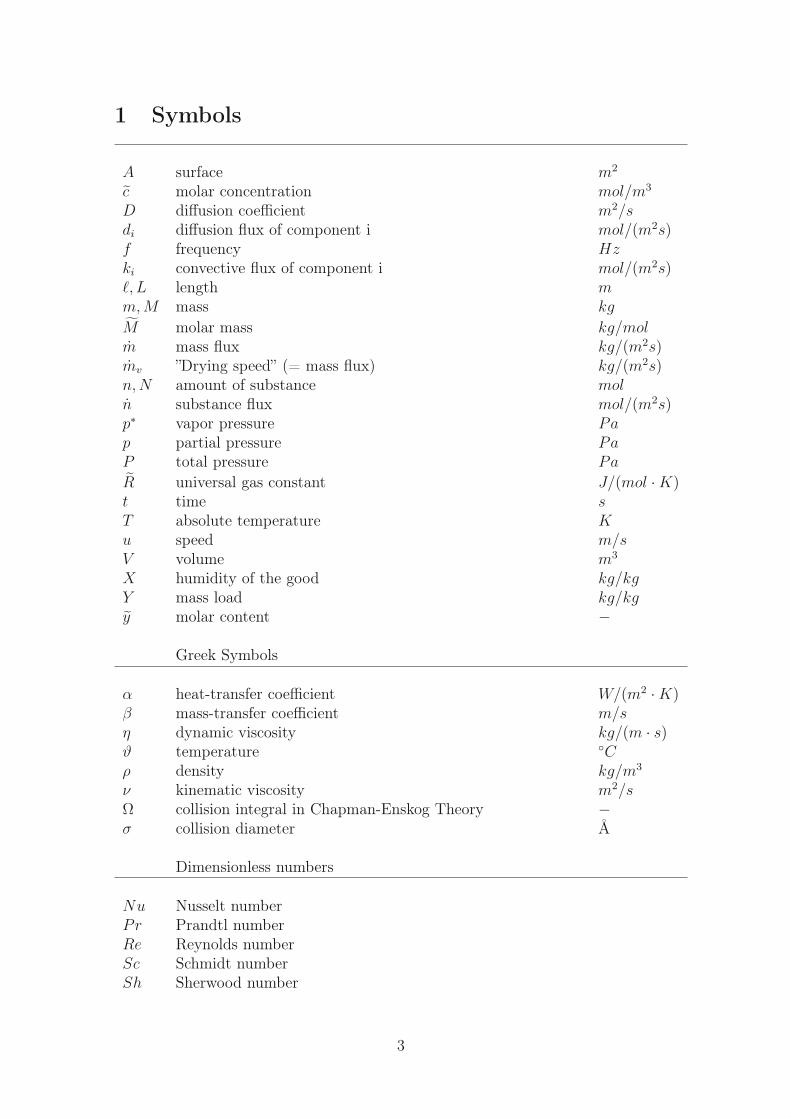
1 Symbols

A surface m2

c molar concentration mol/m3

D diffusion coefficient m2/sdi diffusion flux of component i mol/(m2s)f frequency Hzki convective flux of component i mol/(m2s)ℓ, L length mm,M mass kg

M molar mass kg/molm mass flux kg/(m2s)mv ”Drying speed” (= mass flux) kg/(m2s)n,N amount of substance moln substance flux mol/(m2s)p∗ vapor pressure Pap partial pressure PaP total pressure Pa

R universal gas constant J/(mol ·K)t time sT absolute temperature Ku speed m/sV volume m3

X humidity of the good kg/kgY mass load kg/kgy molar content −

Greek Symbols

α heat-transfer coefficient W/(m2 ·K)β mass-transfer coefficient m/sη dynamic viscosity kg/(m · s)ϑ temperature Cρ density kg/m3

ν kinematic viscosity m2/sΩ collision integral in Chapman-Enskog Theory −σ collision diameter Å

Dimensionless numbers

Nu Nusselt numberPr Prandtl numberRe Reynolds numberSc Schmidt numberSh Sherwood number

3

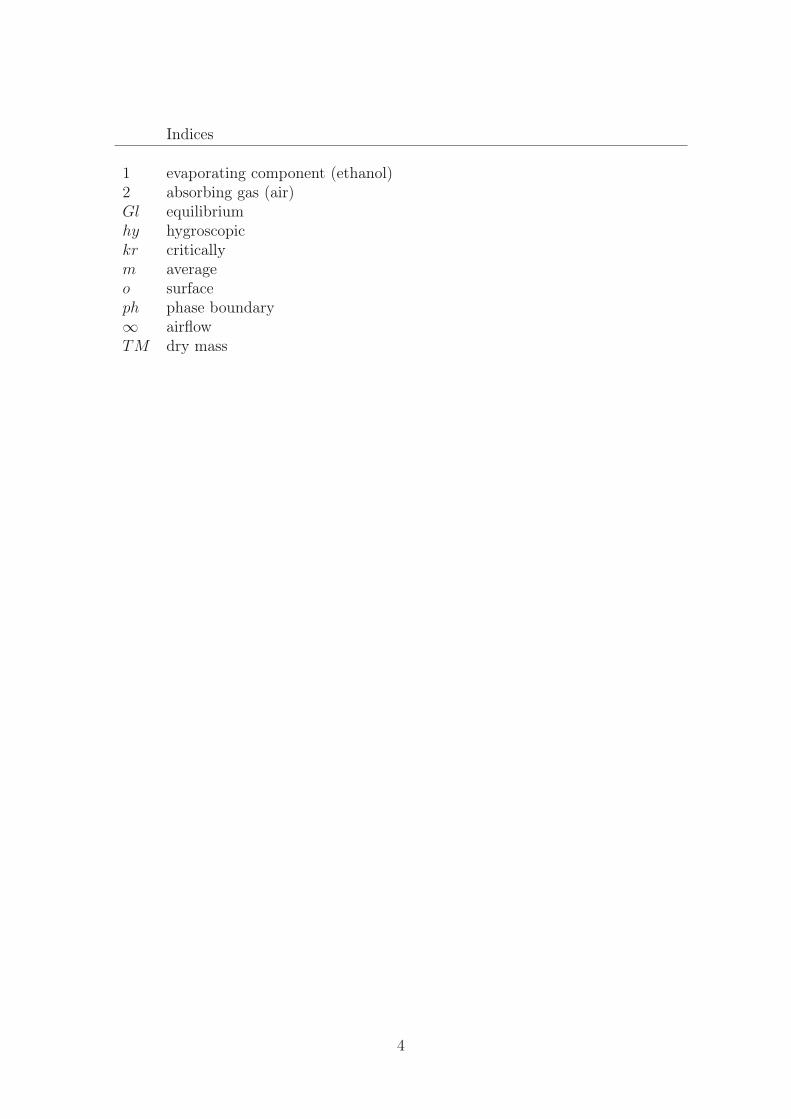
Indices

1 evaporating component (ethanol)2 absorbing gas (air)Gl equilibriumhy hygroscopickr criticallym averageo surfaceph phase boundary∞ airflowTM dry mass

4

2 Fundamentals of drying

There is currently no English version of this chapter in this script. Please see theGerman version or the relevant chapters on drying (Ch.1 to 1.3) in "Ullmann’s En-cyclopedia of Industrial Chemistry" You can find it online via www.ethbib.ethz.ch orask the teaching assistant for a copy.

5

3 The drying apparatus used in the lab course

3.1 Drying unit

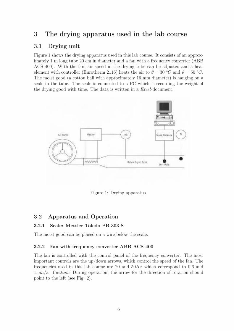
Figure 1 shows the drying apparatus used in this lab course. It consists of an approx-imately 1 m long tube 20 cm in diameter and a fan with a frequency converter (ABBACS 400). With the fan, air speed in the drying tube can be adjusted and a heatelement with controller (Eurotherm 2116) heats the air to ϑ = 30 oC and ϑ = 50 oC.The moist good (a cotton ball with approximately 16 mm diameter) is hanging on ascale in the tube. The scale is connected to a PC which is recording the weight ofthe drying good with time. The data is written in a Excel -document.

Figure 1: Drying apparatus.

3.2 Apparatus and Operation

3.2.1 Scale: Mettler Toledo PB-303-S

The moist good can be placed on a wire below the scale.

3.2.2 Fan with frequency converter ABB ACS 400

The fan is controlled with the control panel of the frequency converter. The mostimportant controls are the up/down arrows, which control the speed of the fan. Thefrequencies used in this lab course are 20 and 50Hz which correspond to 0.6 and1.5m/s. Caution: During operation, the arrow for the direction of rotation shouldpoint to the left (see Fig. 2).

6

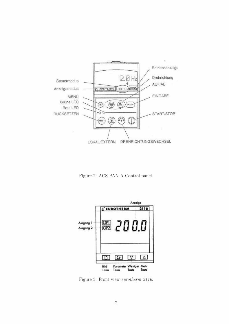
Figure 2: ACS-PAN-A-Control panel.

Figure 3: Front view eurotherm 2116.

7

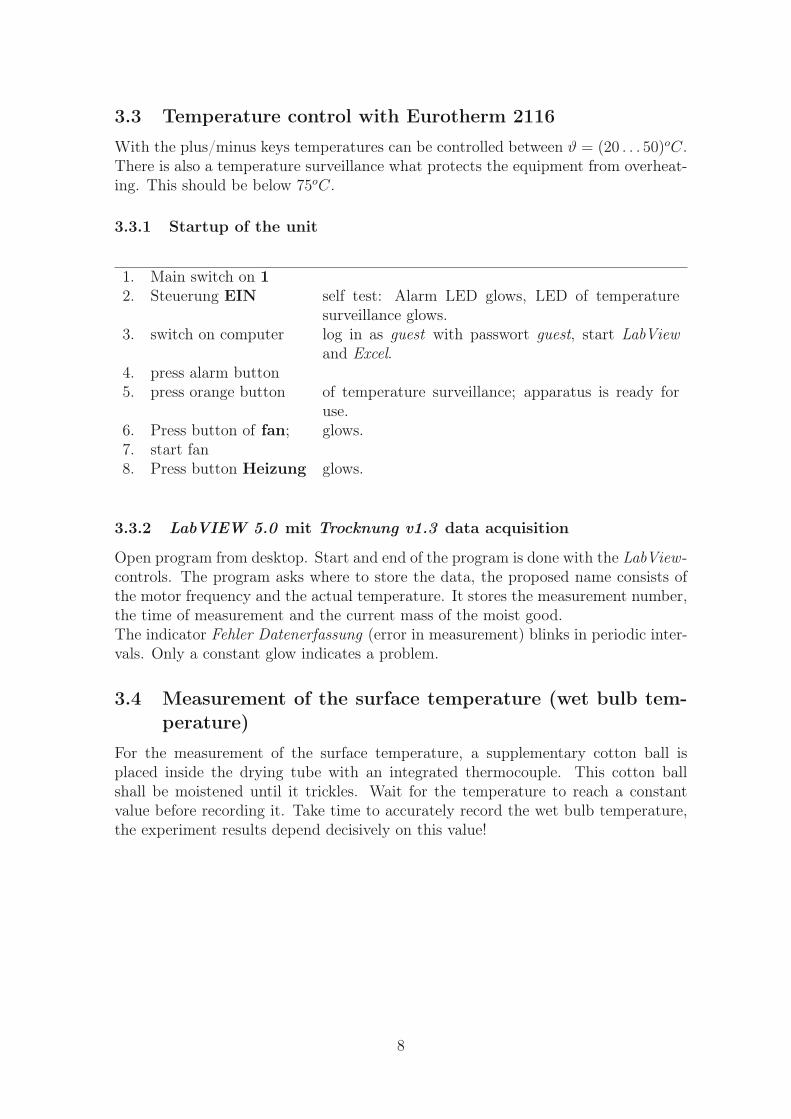
3.3 Temperature control with Eurotherm 2116

With the plus/minus keys temperatures can be controlled between ϑ = (20 . . . 50)oC.There is also a temperature surveillance what protects the equipment from overheat-ing. This should be below 75oC.

3.3.1 Startup of the unit

1. Main switch on 12. Steuerung EIN self test: Alarm LED glows, LED of temperature

surveillance glows.3. switch on computer log in as guest with passwort guest, start LabView

and Excel.4. press alarm button5. press orange button of temperature surveillance; apparatus is ready for

use.6. Press button of fan; glows.7. start fan8. Press button Heizung glows.

3.3.2 LabVIEW 5.0 mit Trocknung v1.3 data acquisition

Open program from desktop. Start and end of the program is done with the LabView -controls. The program asks where to store the data, the proposed name consists ofthe motor frequency and the actual temperature. It stores the measurement number,the time of measurement and the current mass of the moist good.The indicator Fehler Datenerfassung (error in measurement) blinks in periodic inter-vals. Only a constant glow indicates a problem.

3.4 Measurement of the surface temperature (wet bulb tem-perature)

For the measurement of the surface temperature, a supplementary cotton ball isplaced inside the drying tube with an integrated thermocouple. This cotton ballshall be moistened until it trickles. Wait for the temperature to reach a constantvalue before recording it. Take time to accurately record the wet bulb temperature,the experiment results depend decisively on this value!

8

4 Tasks

The moist good will be soaked in ethanol. The weight change during the dryingprocess is determined for different air velocities and temperatures. From the ob-tained data, the individual drying rates for the first drying period is determined andcompared to theory.

1. Determine weight vs. time of the wet cotton ball for a constant air temperatureof 30oC and different air speeds of u = 0.58 m/s, 0.87 m/s, 1.16 m/s and 1.45m/s. These correspond to the fan frequencies of f = 20 Hz, 30 Hz, 40 Hz and50 Hz respectively.

2. Analogous point 1, but with a constant temperature of 50oC.

3. Determine the drying rates in the first period of drying from the obtained dataand plot these as a function of air velocity. Discuss your results.

4. Make an other experiment with the temperature of 50oC and air speed of 1.45m/s, but this time use another material than cotton. (Lava stone or pumicestone) Here the drying progression must be recorded until the second periodof drying. (Happens very fast!) (select a smaller time step for recording)Compare this result to the precedent result of the cotton ball with the sameconditions.

5. Calculate the drying speeds of the first period of drying for all the experimentalconditions with the theory given in the appendix. First, determine the Reynoldsnumber and find out which correlation is suitable for determining the masstransfer coefficient. Compare your theoretical results with the experimentalvalues.

6. Write a detailed report of the results from point 1 to 5. The teaching assistantwill hand out guidelines for the writing of the report.

9

References

[1] E. L. Cussler. Diffusion - Mass Transfer in Fluid Systems. Cambridge, 2ndedition, 1997.

[2] V. Gnielinski, A. Mersmann, and F. Thurner. Verdampfung, Kristallisation,

Trocknung. Vieweg, Wiesbaden, 1993.

[3] Landolt-Börnstein, volume 2, Bandteil b. Springer, Berlin, 1962.

[4] VDI-Wärmeatlas, volume 6. VDI Verlag, Düsseldorf, 1991.

[5] H. Grassmann, P. Widmer und F. Sinn. Einführung in die Thermische Ver-

fahrenstechnik. Walter de Gruyter, Berlin, 3rd edition, 1997.

[6] E.-U. Schlünder. Einführung in die Stoffübertragung. Vieweg, Braunschweig,1996.

[7] E.-U. Schlünder and M. Holger. Einführung in Die Wärmeübertragung. Vieweg,Braunschweig, 1995.

[8] H. A. Vauck, W. R. A. und Müller. Grundoperationen Chemischer Verfahren-

stechnik. Deutscher Verlag für Grundstoffindustrie, Leipzig, 10th edition, 1994.

[9] Vorlesungsskript. Mechanische Verfahrenstechnik I. Institut für Verfahrenstech-nik, ETHZ, 1998.

10

Appendix

A Calculation of the drying speed of the first drying

period

In the following section a relation to calculate the drying speed will be derived. (see[6]).Accoring to basic equation of diffusion the flux nj is:

nj = −Dj,k∂cj∂z

(1)

Equation 1 is valid for all components, i.e. in our case for the evaporating ethanol (1)and the uptaking gas air(2). The sum of partial pressures is equal to total pressure

P = p1 + p2 (2)

Thus

∂c1∂z

+∂c2∂z

= 0 (3)

This means, the flux of ethanol vapor is balanced with a flux of air. The phaseboundary ethanol-air is permeable for ethanol but not for air, so that the flux of airhas to be zero at this boundary even though a concentration gradient is present. Thisleads to the assumption that the evaporation is not only diffusion driven, but thereis also a convection part. The component flux nj consists of diffusion flux dj and aconvection flux kj.

nj = dj + kj = −ρgDj,k∂yj∂z

+ nyj (4)

Applied on the investigated evaporation of ethanol(1) in air(2):

n1 = −ρgD1,2∂y1∂z

+ ny1 (5)

n2 = −ρgD1,2∂y2∂z

+ ny2 (6)

The phase boundary is impermeable for air (semipermeable wall), i.e. on the phaseboundary:

n2 = 0 (7)

The sum of all component flux is equal to total flux. n:

11

n1 + n2 = n (8)

Hence for the ethanol flux on the phase boundary:

n1 = n (9)

With eq. 9 eq. 5 becomes:

n1(1− y1) = −ρgD1,2∂y1∂z

(10)

Integration from z = 0 to z = ℓ and with following boundary conditions:

z = 0⇒ y1 = y1,ph (11)

z = ℓ⇒ y1 = y1,ℓ (12)

eq. 10 becomes:

n1 = ρgD1,2

ℓln

1− y1,ℓ1− y1,ph

(13)

The length ℓ is specific to the process and mostly unknown. The factor D1,2

ℓis re-

placed by the mass transfer coefficient β which is determined by empirical correlationsspecific to the process. The mass transfer coefficient β is defined as follows:

β =Sh ·D1,2

L(14)

With Sherwood’s number Sh, the diffusion coefficient D1,2 and the characteristiclength L, which is in our case the diameter of the cotton ball. Applying analogybetween mass- and heat transfer, following correlation for Sherwood’s number for ansphere in a flow field can be found [4]: (for 1 ≤ Re ≤ 106)

Sh = 2 +√Sh2

lam + Sh2turb (15)

with

Shlam = 0.664Sc1

3Re1

2 (16)

and

Shturb =0.037ScRe

4

5

1 + 2.443Re−0.1(Sc2

3 − 1)(17)

12

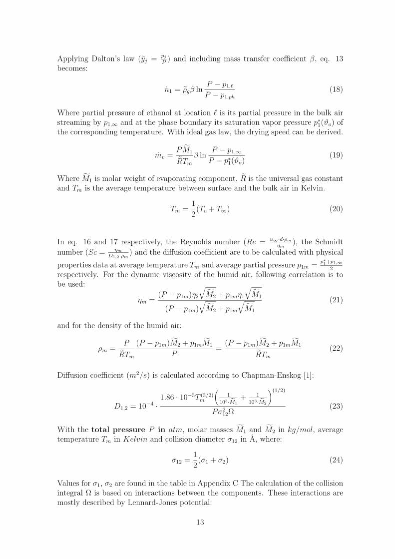
Applying Dalton’s law (yj = pjP) and including mass transfer coefficient β, eq. 13

becomes:

n1 = ρgβ lnP − p1,ℓP − p1,ph

(18)

Where partial pressure of ethanol at location ℓ is its partial pressure in the bulk airstreaming by p1,∞ and at the phase boundary its saturation vapor pressure p∗1(ϑo) ofthe corresponding temperature. With ideal gas law, the drying speed can be derived.

mv =PM1

RTm

β lnP − p1,∞P − p∗1(ϑo)

(19)

Where M1 is molar weight of evaporating component, R is the universal gas constantand Tm is the average temperature between surface and the bulk air in Kelvin.

Tm =1

2(To + T∞) (20)

In eq. 16 and 17 respectively, the Reynolds number (Re = u∞·d·ρmηm

), the Schmidtnumber (Sc = ηm

D1,2·ρm) and the diffusion coefficient are to be calculated with physical

properties data at average temperature Tm and average partial pressure p1m =p∗1+p1,∞2

respectively. For the dynamic viscosity of the humid air, following correlation is tobe used:

ηm =(P − p1m)η2

√M2 + p1mη1

√M1

(P − p1m)√M2 + p1m

√M1

(21)

and for the density of the humid air:

ρm =P

RTm

(P − p1m)M2 + p1mM1

P=

(P − p1m)M2 + p1mM1

RTm

(22)

Diffusion coefficient (m2/s) is calculated according to Chapman-Enskog [1]:

D1,2 = 10−4 ·1.86 · 10−3T (3/2)

m

(1

103·M1

+ 1

103·M2

)(1/2)

Pσ212Ω

(23)

With the total pressure P in atm, molar masses M1 and M2 in kg/mol, averagetemperature Tm in Kelvin and collision diameter σ12 in Å, where:

σ12 =1

2(σ1 + σ2) (24)

Values for σ1, σ2 are found in the table in Appendix C The calculation of the collisionintegral Ω is based on interactions between the components. These interactions aremostly described by Lennard-Jones potential:

13

ǫ12 =√ǫ1ǫ2 (25)

Values for ǫi are in the table in Appendix C. With known ǫ12, Ω as a function of ǫ12kBT

can be found in the table in Appendix D.

14

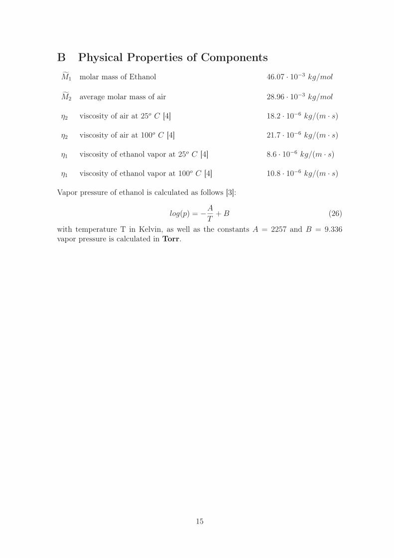
B Physical Properties of Components

M1 molar mass of Ethanol 46.07 · 10−3 kg/mol

M2 average molar mass of air 28.96 · 10−3 kg/mol

η2 viscosity of air at 25o C [4] 18.2 · 10−6 kg/(m · s)

η2 viscosity of air at 100o C [4] 21.7 · 10−6 kg/(m · s)

η1 viscosity of ethanol vapor at 25o C [4] 8.6 · 10−6 kg/(m · s)

η1 viscosity of ethanol vapor at 100o C [4] 10.8 · 10−6 kg/(m · s)

Vapor pressure of ethanol is calculated as follows [3]:

log(p) = −A

T+B (26)

with temperature T in Kelvin, as well as the constants A = 2257 and B = 9.336vapor pressure is calculated in Torr.

15

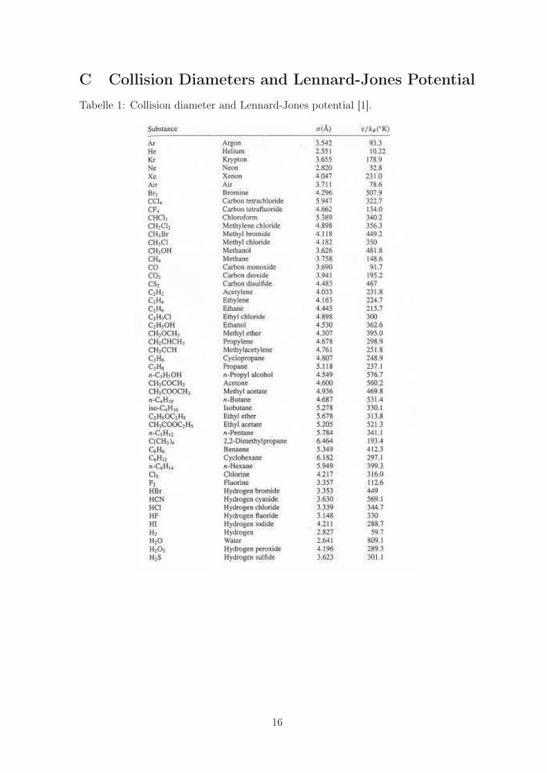
C Collision Diameters and Lennard-Jones Potential

Tabelle 1: Collision diameter and Lennard-Jones potential [1].

16

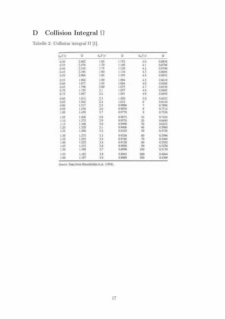
D Collision Integral Ω

Tabelle 2: Collision integral Ω [1].

17