Dr. Ahmad Ibrahim MosaMinistry Advisor for Transportation Planning

Director of Transportation Planning Center of Excellence – Associate Professor, German University, Cairo

BIG DATA AND URBAN MOBILITY

Cairo Transport and Big Data

Mobility Figures for GCMA

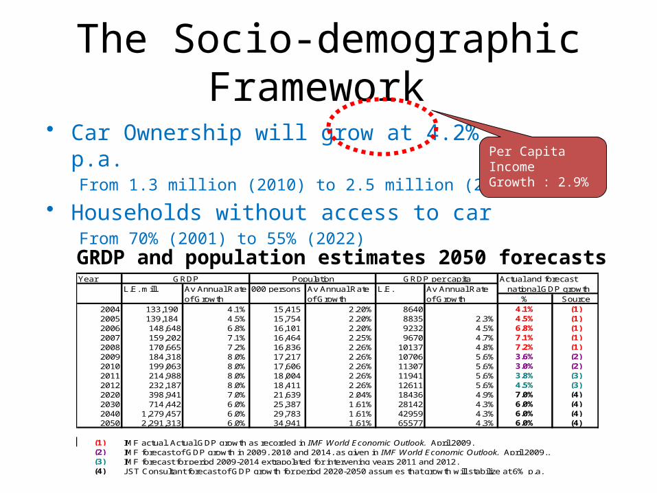
The Socio-demographic Framework

Year Actual and forecast L.E. mill. Av Annual Rate 000 persons Av Annual Rate L.E. Av Annual Rate

of Growth of Growth of Growth % Source2004 133,190 4.1% 15,415 2.20% 8640 4.1% (1)2005 139,184 4.5% 15,754 2.20% 8835 2.3% 4.5% (1)2006 148,648 6.8% 16,101 2.20% 9232 4.5% 6.8% (1)2007 159,202 7.1% 16,464 2.25% 9670 4.7% 7.1% (1)2008 170,665 7.2% 16,836 2.26% 10137 4.8% 7.2% (1)2009 184,318 8.0% 17,217 2.26% 10706 5.6% 3.6% (2)2010 199,063 8.0% 17,606 2.26% 11307 5.6% 3.0% (2)2011 214,988 8.0% 18,004 2.26% 11941 5.6% 3.8% (3)2012 232,187 8.0% 18,411 2.26% 12611 5.6% 4.5% (3)2020 398,941 7.0% 21,639 2.04% 18436 4.9% 7.0% (4)2030 714,442 6.0% 25,387 1.61% 28142 4.3% 6.0% (4)2040 1,279,457 6.0% 29,783 1.61% 42959 4.3% 6.0% (4)2050 2,291,313 6.0% 34,941 1.61% 65577 4.3% 6.0% (4)

(1) IMF actual. Actual GDP growth as recorded in IMF World Economic Outlook, April 2009.(2) IMF forecast of GDP growth in 2009, 2010 and 2014, as given in IMF World Economic Outlook, April 2009..(3) IMF forecast for period 2009-2014 extrapolated for intervening years 2011 and 2012. (4) JST Consultant forecast of GDP growth for period 2020-2050 assumes that growth will stabilize at 6% p.a.

GRDP Population GRDP per capitanational GDP growth

GRDP and population estimates 2050 forecasts

• Car Ownership will grow at 4.2% p.a.From 1.3 million (2010) to 2.5 million (2022)

• Households without access to carFrom 70% (2001) to 55% (2022)

Per Capita Income Growth : 2.9%

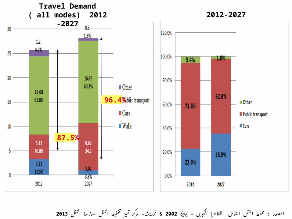
Travel Demand ( all modes) 2012 -2027 2012-2027

87.5%

96.4%

جايكا : – الكبري للقاهرة الشامل النقل مخطط – – 2002المصدر النقل وزارة النقل تخطيط تميز مركز تحديث &2013

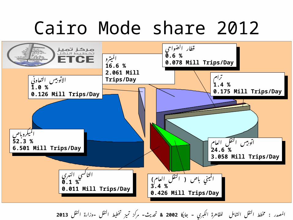
Cairo Mode share 2012Data source: JICA Study Team. Data exclude Maadi and refer to unlinked trips derived from HIS prior to

network calibration procedures.

Shared Taxi52.3 %6.501Mill Trips/Day

الميكروباص52.3 %6.501 Mill Trips/Day Shared Taxi

52.3 %6.501Mill Trips/Day

العام النقل اتوبيس24.6 %3.058 Mill Trips/Day

الميترو16.6 %2.061 Mill Trips/Day

التعاوني االتوبيس1.0 %0.126 Mill Trips/Day

Shared Taxi52.3 %6.501Mill Trips/Day

الضواحي قطار0.6 %0.078 Mill Trips/Day

Shared Taxi52.3 %6.501Mill Trips/Day

ترام1.4 %0.175 Mill Trips/Day

Shared Taxi52.3 %6.501Mill Trips/Day

النقل ) باص المينيالعام(3.4 %0.426 Mill Trips/Day

Shared Taxi52.3 %6.501Mill Trips/Day

النهري التاكسي0.1 %0.011 Mill Trips/Day

جايكا : – الكبري للقاهرة الشامل النقل مخطط – – 2002المصدر النقل وزارة النقل تخطيط تميز مركز تحديث &2013

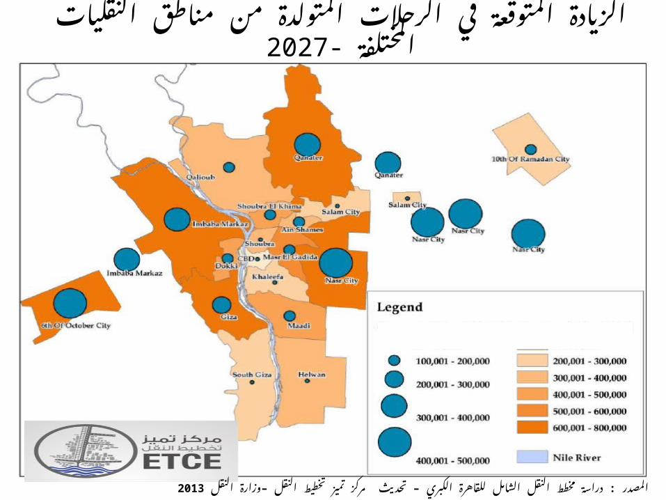
النقليات مناطق من المتولدة الرحالت في المتوقعة الزيادة2027المختلفة -

النقل : – – وزارة النقل تخطيط تميز مركز تحديث الكبري للقاهرة الشامل النقل مخطط دراسة 2013المصدر

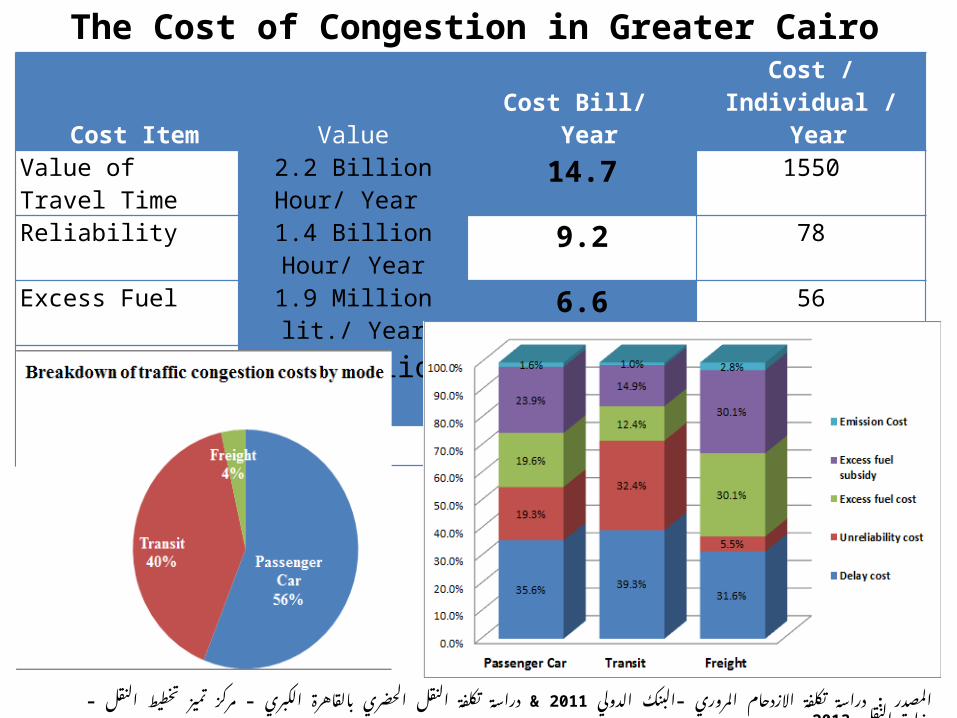
Cost Item Value Cost Bill/ Year

Cost / Individual / Year

Value of Travel Time 2.2 Billion Hour/ Year 14.7 1550

Reliability 1.4 Billion Hour/ Year 9.2 78

Excess Fuel 1.9 Million lit./ Year 6.6 56

CO2 Emissions 7.1 Billion kg 0.4 5

Total – 30.8 1689

The Cost of Congestion in Greater Cairo

الدولي : – البنك المروري االزدحام تكلفة دراسة الكبري – 2011المصدر بالقاهرة الحضري النقل تكلفة دراسة &النقل – وزارة النقل تخطيط تميز 2013مركز

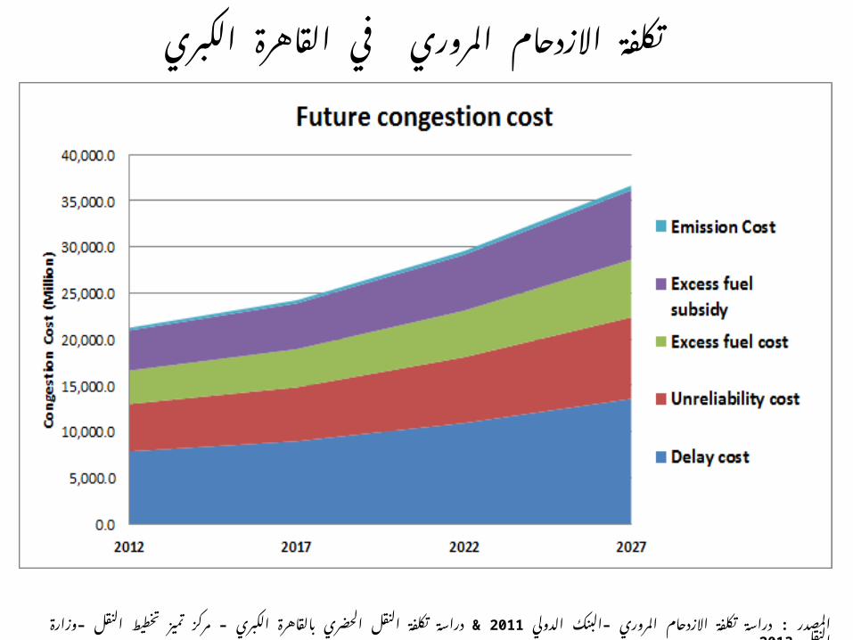
الكبري القاهرة في المروري االزدحام تكلفة

الدولي : – البنك المروري االزدحام تكلفة دراسة مركز – 2011المصدر الكبري بالقاهرة الحضري النقل تكلفة دراسة &النقل – وزارة النقل تخطيط 2013تميز

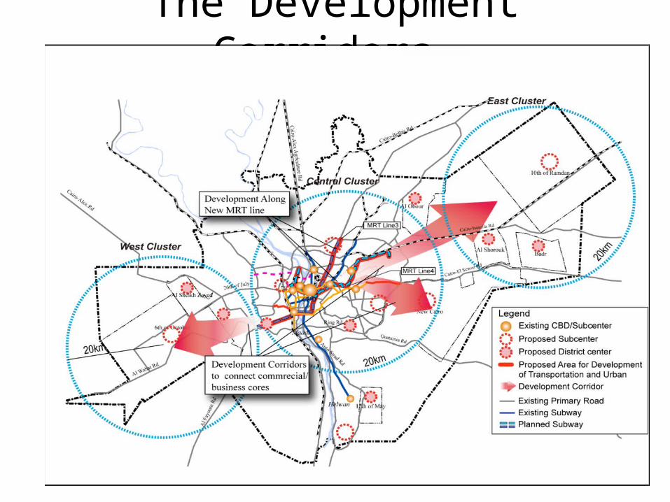
The Development Corridors

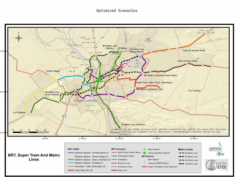
Optimized Scenarios

Types of Data Needed

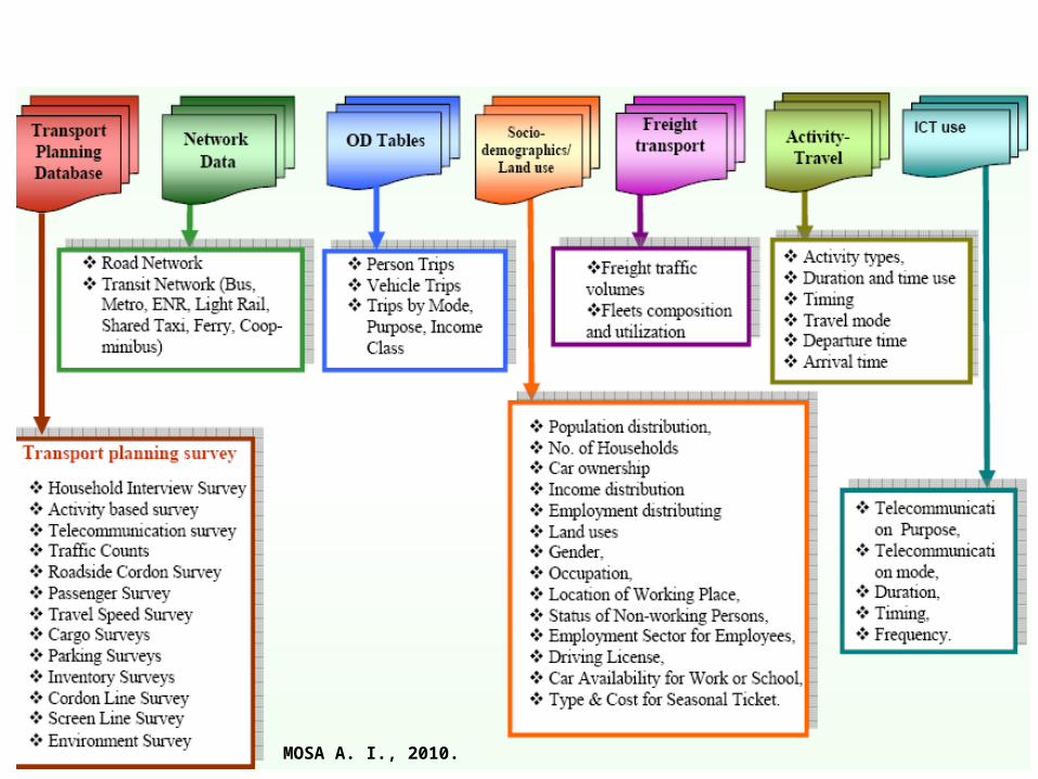
12MOSA A. I., 2010.

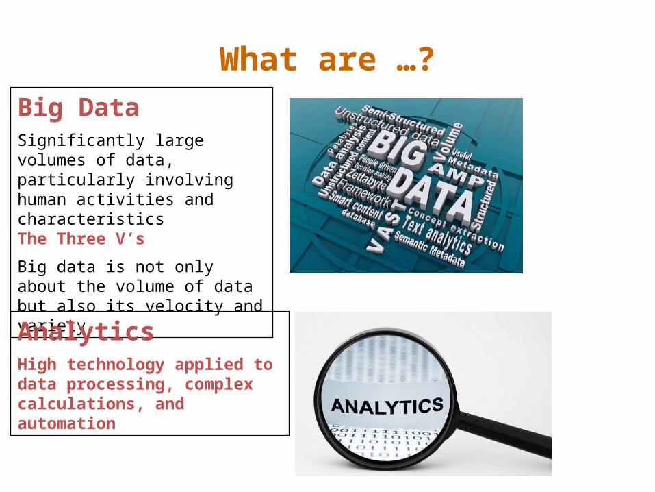
What are …?Big DataSignificantly large volumes of data, particularly involving human activities and characteristicsThe Three V’s

Big data is not only about the volume of data but also its velocity and variety

AnalyticsHigh technology applied to data processing, complex calculations, and automation

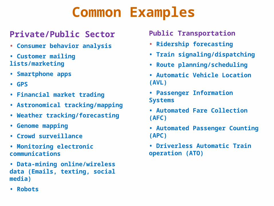
Common Examples

Private/Public Sector• Consumer behavior analysis

• Customer mailing lists/marketing

• Smartphone apps

• GPS

• Financial market trading

• Astronomical tracking/mapping

• Weather tracking/forecasting

• Genome mapping

• Crowd surveillance

• Monitoring electronic communications

• Data-mining online/wireless data (Emails, texting, social media)

• Robots

Public Transportation

• Ridership forecasting

• Train signaling/dispatching

• Route planning/scheduling

• Automatic Vehicle Location (AVL)

• Passenger Information Systems

• Automated Fare Collection (AFC)

• Automated Passenger Counting (APC)

• Driverless Automatic Train operation (ATO)

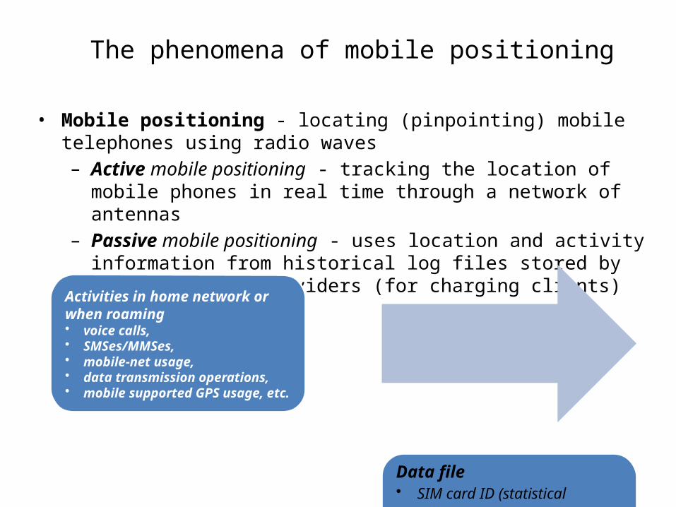
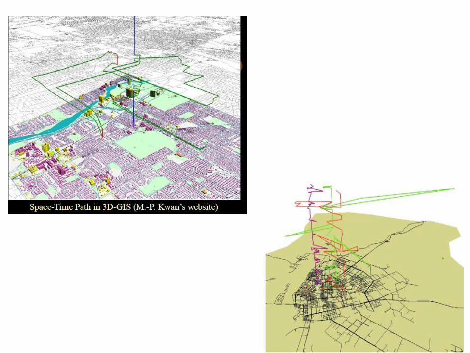
The phenomena of mobile positioning

• Mobile positioning - locating (pinpointing) mobile telephones using radio waves– Active mobile positioning - tracking the location of mobile phones in real

time through a network of antennas– Passive mobile positioning - uses location and activity information from

historical log files stored by mobile service providers (for charging clients)

15

Activities in home network or when roaming• voice calls, • SMSes/MMSes, • mobile-net usage, • data transmission operations, • mobile supported GPS usage, etc.

Data file• SIM card ID (statistical

pseudonym) • Date and time • Antenna ID with location data • Country ID

16

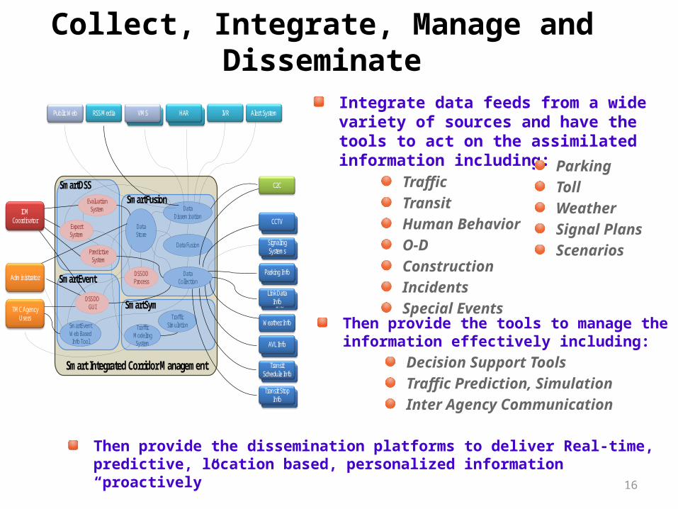
Collect, Integrate, Manage and Disseminate

Integrate data feeds from a wide variety of sources and have the tools to act on the assimilated information including:

TrafficTransitHuman BehaviorO-D ConstructionIncidentsSpecial Events

ParkingTollWeatherSignal PlansScenarios

Then provide the tools to manage the information effectively including:

Decision Support ToolsTraffic Prediction, SimulationInter Agency Communication

Then provide the dissemination platforms to deliver Real-time, predictive, location based, personalized information “proactively”

SmartDSS

SmartSym

SmartEvent

SmartFusion

Expert System

EvaluationSystem

Predictive System

Traffic Modeling

System

Traffic Simulation

DSS DD Process

Data Store

Data Dissemination

Data Fusion

Data Collection

DSS DD GUI

SmartEventWeb Based

Info Tool

RSS Media Alert SystemPublic Web IVR

Parking Info

Link Data Info

Link Data Info

Parking Info

Weather InfoAVL Info

Weather InfoTransit

Schedule Info

Weather InfoTransit Stop

Info

Parking InfoSignaling Systems

Parking Info

Parking InfoHARParking InfoVMS

Weather Info

CCTV

C2C

Smart Integrated Corridor Management

TMC Agency Users

Administrator

ICM Coordinator

Big Data Is Needed For Cairo

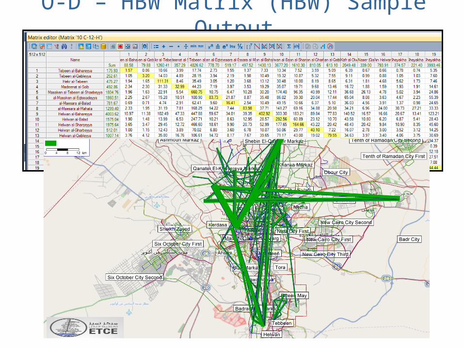
O-D – HBW Matrix (HBW) Sample Output

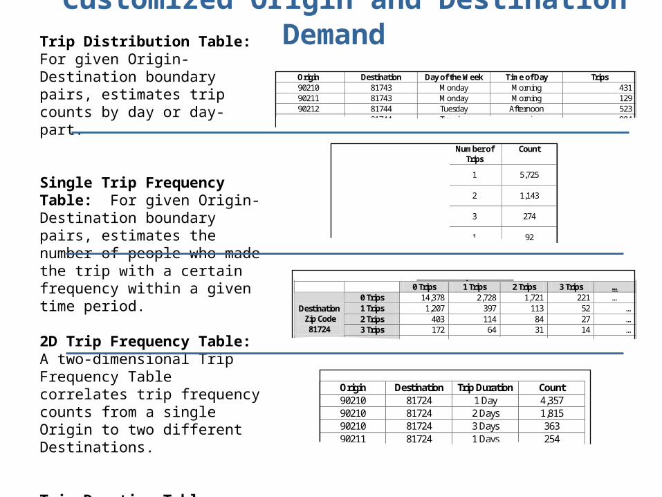
Trip Distribution Table: For given Origin- Destination boundary pairs, estimates trip counts by day or day-part.

Single Trip Frequency Table: For given Origin-Destination boundary pairs, estimates the number of people who made the trip with a certain frequency within a given time period.

2D Trip Frequency Table: A two-dimensional Trip Frequency Table correlates trip frequency counts from a single Origin to two different Destinations.

Trip Duration Table: Estimates the number of people who made trips of various durations between given Origin-Destination boundary pairs.

Origin Destination Day of the Week Time of Day Trips 90210 81743 Monday Morning 431 90211 81743 Monday Morning 129 90212 81744 Tuesday Afternoon 523 90213 81744 Tuesday Evening 904

Number of Trips

Count

1 5,725

2 1,143

3 274

1 92

2 27

Destination Zip Code 90381 0 Trips 1 Trips 2 Trips 3 Trips …

0 Trips 14,378 2,728 1,721 221 … 1 Trips 1,207 397 113 52 … 2 Trips 403 114 84 27 … 3 Trips 172 64 31 14 …

Destination Zip Code

81724 … … … … … …

Origin Destination Trip Duration Count 90210 81724 1 Day 4,357 90210 81724 2 Days 1,815 90210 81724 3 Days 363 90211 81724 1 Days 254 90211 81724 2 Days 109

Customized Origin and Destination Demand

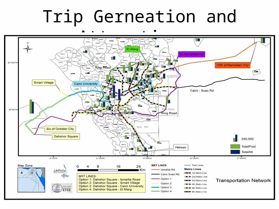
Trip Gerneation and Attraction

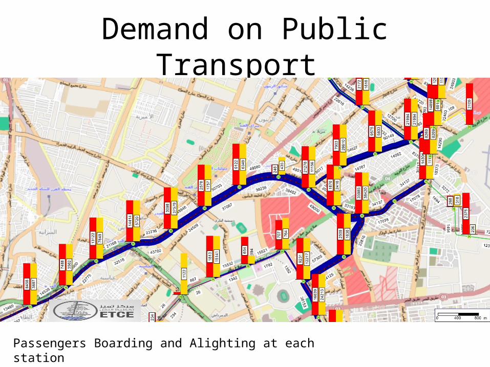
Demand on Public Transport

Passengers Boarding and Alighting at each station

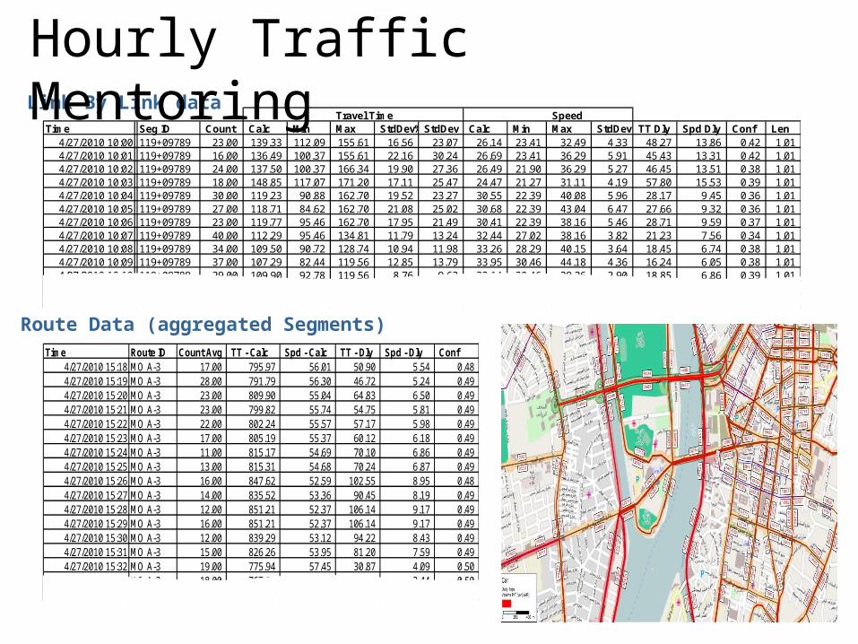
Travel Time SpeedTime Seg NumSeg ID Count Calc Min Max StdDev%StdDev Calc Min Max StdDev TT Dly Spd Dly Conf Len

4/27/2010 10:00 119+09789 23.00 139.33 112.09 155.61 16.56 23.07 26.14 23.41 32.49 4.33 48.27 13.86 0.42 1.01 4/27/2010 10:01 119+09789 16.00 136.49 100.37 155.61 22.16 30.24 26.69 23.41 36.29 5.91 45.43 13.31 0.42 1.01 4/27/2010 10:02 119+09789 24.00 137.50 100.37 166.34 19.90 27.36 26.49 21.90 36.29 5.27 46.45 13.51 0.38 1.01 4/27/2010 10:03 119+09789 18.00 148.85 117.07 171.20 17.11 25.47 24.47 21.27 31.11 4.19 57.80 15.53 0.39 1.01 4/27/2010 10:04 119+09789 30.00 119.23 90.88 162.70 19.52 23.27 30.55 22.39 40.08 5.96 28.17 9.45 0.36 1.01 4/27/2010 10:05 119+09789 27.00 118.71 84.62 162.70 21.08 25.02 30.68 22.39 43.04 6.47 27.66 9.32 0.36 1.01 4/27/2010 10:06 119+09789 23.00 119.77 95.46 162.70 17.95 21.49 30.41 22.39 38.16 5.46 28.71 9.59 0.37 1.01 4/27/2010 10:07 119+09789 40.00 112.29 95.46 134.81 11.79 13.24 32.44 27.02 38.16 3.82 21.23 7.56 0.34 1.01 4/27/2010 10:08 119+09789 34.00 109.50 90.72 128.74 10.94 11.98 33.26 28.29 40.15 3.64 18.45 6.74 0.38 1.01 4/27/2010 10:09 119+09789 37.00 107.29 82.44 119.56 12.85 13.79 33.95 30.46 44.18 4.36 16.24 6.05 0.38 1.01 4/27/2010 10:10 119+09789 29.00 109.90 92.78 119.56 8.76 9.63 33.14 30.46 39.26 2.90 18.85 6.86 0.39 1.01

Link By Link data

Route Data (aggregated Segments)Time Route ID Count Avg TT - Calc Spd - Calc TT - Dly Spd - Dly Conf

4/27/2010 15:18 MO A-3 17.00 795.97 56.01 50.90 5.54 0.48 4/27/2010 15:19 MO A-3 28.00 791.79 56.30 46.72 5.24 0.49 4/27/2010 15:20 MO A-3 23.00 809.90 55.04 64.83 6.50 0.49 4/27/2010 15:21 MO A-3 23.00 799.82 55.74 54.75 5.81 0.49 4/27/2010 15:22 MO A-3 22.00 802.24 55.57 57.17 5.98 0.49 4/27/2010 15:23 MO A-3 17.00 805.19 55.37 60.12 6.18 0.49 4/27/2010 15:24 MO A-3 11.00 815.17 54.69 70.10 6.86 0.49 4/27/2010 15:25 MO A-3 13.00 815.31 54.68 70.24 6.87 0.49 4/27/2010 15:26 MO A-3 16.00 847.62 52.59 102.55 8.95 0.48 4/27/2010 15:27 MO A-3 14.00 835.52 53.36 90.45 8.19 0.49 4/27/2010 15:28 MO A-3 12.00 851.21 52.37 106.14 9.17 0.49 4/27/2010 15:29 MO A-3 16.00 851.21 52.37 106.14 9.17 0.49 4/27/2010 15:30 MO A-3 12.00 839.29 53.12 94.22 8.43 0.49 4/27/2010 15:31 MO A-3 15.00 826.26 53.95 81.20 7.59 0.49 4/27/2010 15:32 MO A-3 19.00 775.94 57.45 30.87 4.09 0.50 4/27/2010 15:33 MO A-3 18.00 767.20 58.11 22.13 3.44 0.50 4/27/2010 15:34 MO A-3 8.00 854.43 52.18 109.36 9.37 0.49

Hourly Traffic Mentoring

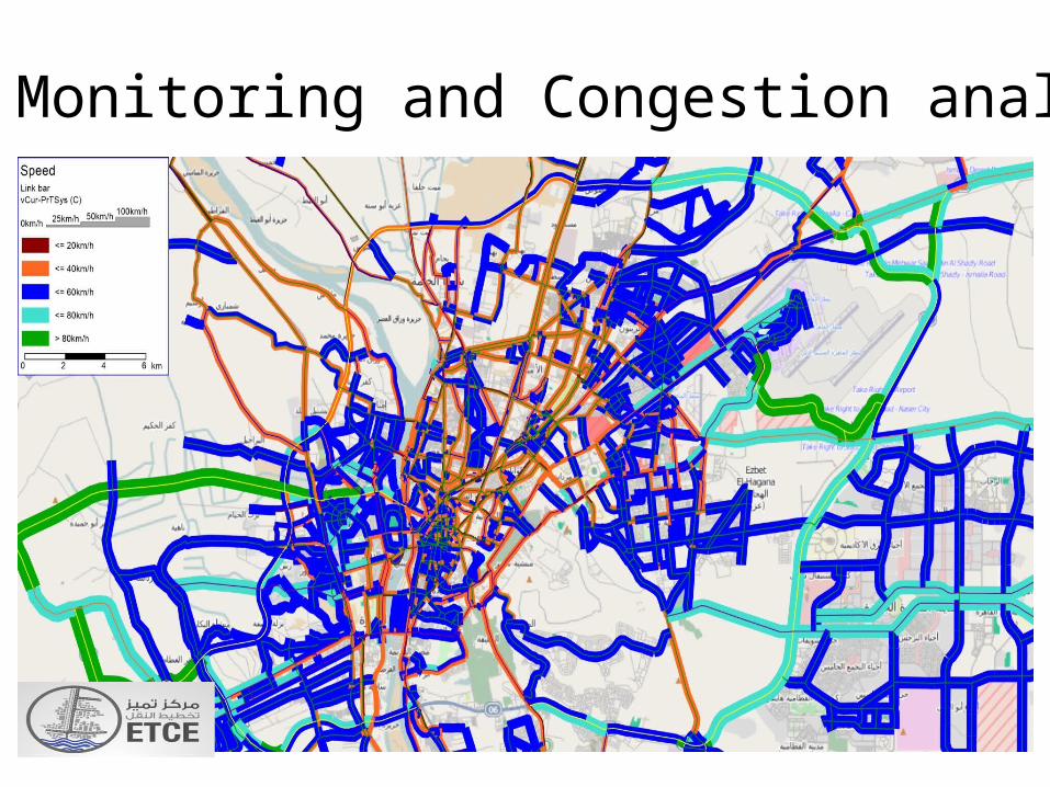
Speed Monitoring and Congestion analysis

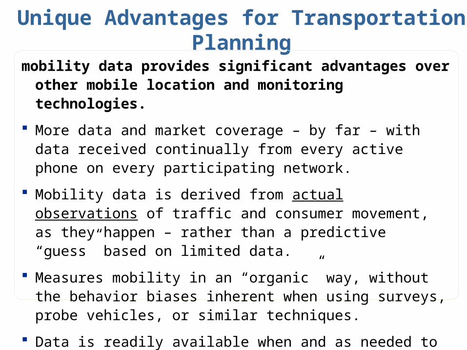
Unique Advantages for Transportation Planning

mobility data provides significant advantages over other mobile location and monitoring technologies.

More data and market coverage – by far – with data received continually from every active phone on every participating network.

Mobility data is derived from actual observations of traffic and consumer movement, as they happen – rather than a predictive “guess” based on limited data.

Measures mobility in an “organic” way, without the behavior biases inherent when using surveys, probe vehicles, or similar techniques.

Data is readily available when and as needed to support either planned or ad hoc project needs.

Big Data would offers significant cost savings – up to 60% or more – versus traditional mobility data collection.

Extracting Vehicular Data From Moving Cell phones on Highways

GUC- Ministry of Transportion TeamAhmed Mosa, Fadwa Fawzy

Proposed Method

• Our method will be explained as follows:

1. Traffic Data Generation.2. Cell Phones Data Generation.3. Dynamic Clustering Algorithm.

• As mentioned before, obtaining vehicle/cell phone data in Egypt is extremely difficult due to security purposes.

• We used " Simulation of Urban MObility" (SUMO) to generate traffic data.

• SUMO is an open source, microscopic, multi-modal traffic simulation. It allows to simulate how a given traffic demand which consists of single vehicles moves through a given road network. The simulation allows to address a large set of traffic management topics. It is purely microscopic in which each vehicle is modeled explicitly, has an own route, and moves individually through the network.

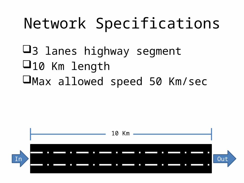
Network Specifications

3 lanes highway segment 10 Km lengthMax allowed speed 50 Km/sec

10 Km

In Out

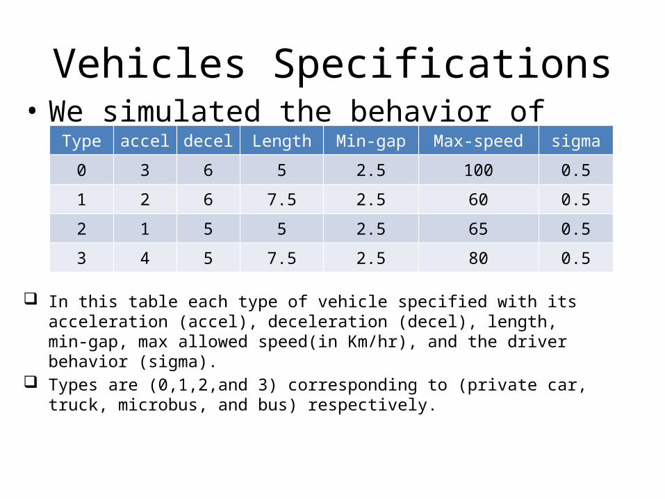
Vehicles Specifications• We simulated the behavior of four types of

vehicles:

In this table each type of vehicle specified with its acceleration (accel), deceleration (decel), length, min-gap, max allowed speed(in Km/hr), and the driver behavior (sigma).

Types are (0,1,2,and 3) corresponding to (private car, truck, microbus, and bus) respectively.

Type accel decel Length Min-gap Max-speed sigma0 3 6 5 2.5 100 0.5

1 2 6 7.5 2.5 60 0.5

2 1 5 5 2.5 65 0.5

3 4 5 7.5 2.5 80 0.5

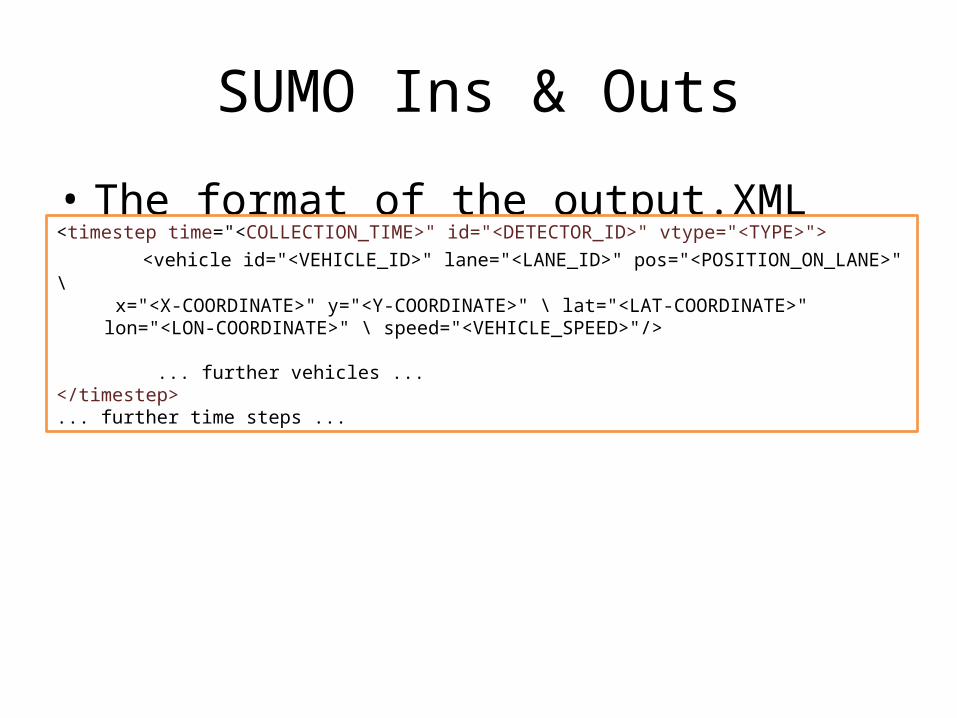
SUMO Ins & Outs

• The format of the output.XML file generated by SUMO is as follows

<timestep time="<COLLECTION_TIME>" id="<DETECTOR_ID>" vtype="<TYPE>"> <vehicle id="<VEHICLE_ID>" lane="<LANE_ID>" pos="<POSITION_ON_LANE>" \

x="<X-COORDINATE>" y="<Y-COORDINATE>" \ lat="<LAT-COORDINATE>" lon="<LON-COORDINATE>" \ speed="<VEHICLE_SPEED>"/>

... further vehicles ... </timestep> ... further time steps ...

XML Parser

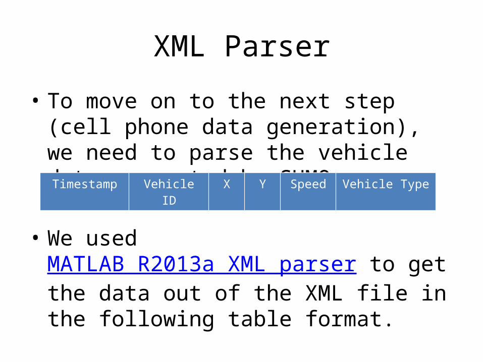
• To move on to the next step (cell phone data generation), we need to parse the vehicle data generated by SUMO.

• We used MATLAB R2013a XML parser to get the data out of the XML file in the following table format.

Timestamp Vehicle ID X Y Speed Vehicle Type

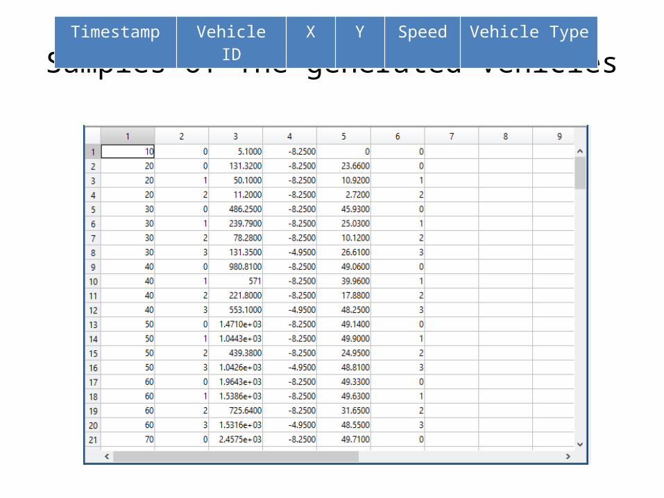
Samples of The generated VehiclesTimestamp Vehicle ID X Y Speed Vehicle Type

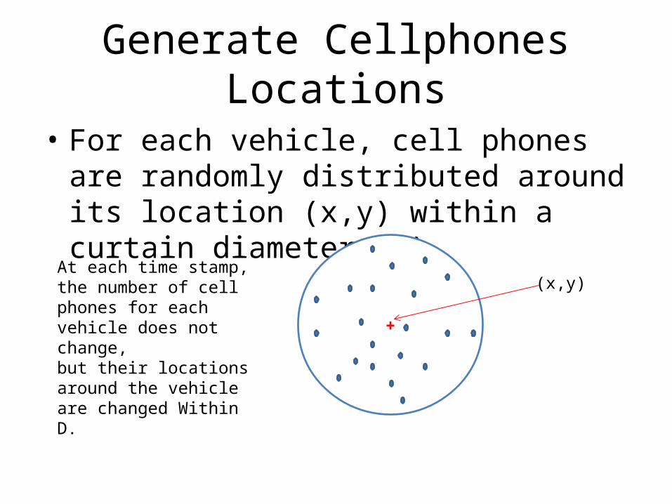
Generate Cellphones Locations

• For each vehicle, cell phones are randomly distributed around its location (x,y) within a curtain diameter (D).

+

(x,y)At each time stamp, the number of cell phones for each vehicle does not change, but their locations around the vehicle are changed Within D.

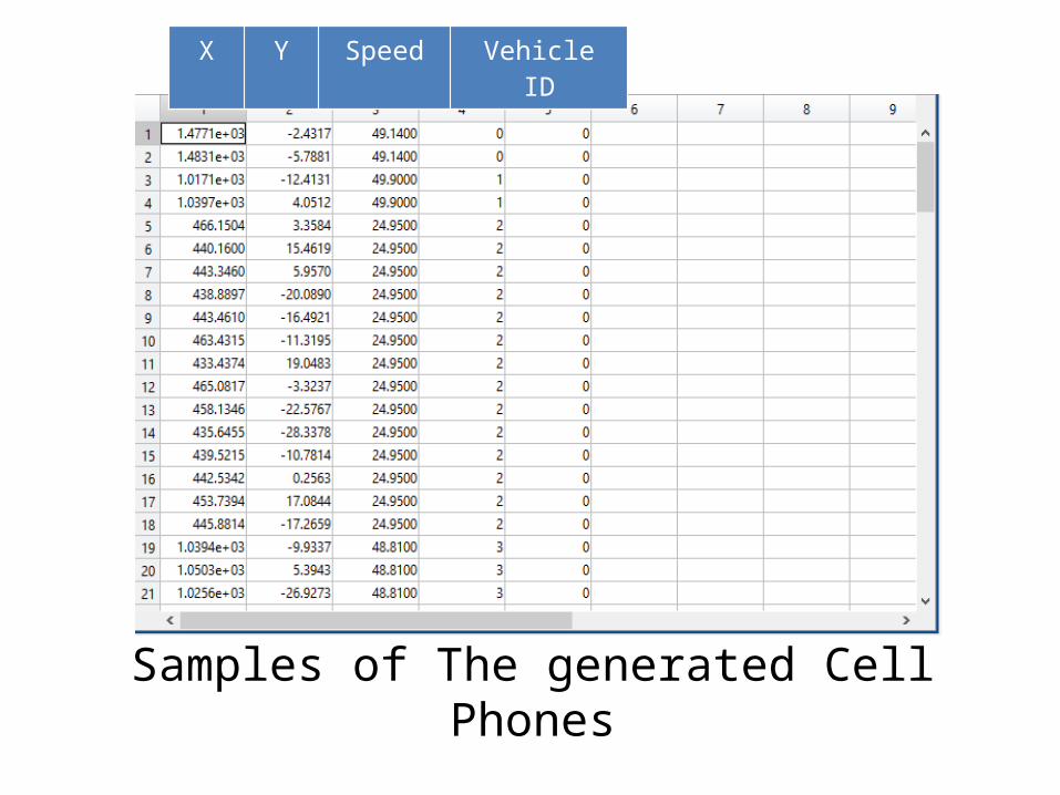
Samples of The generated Cell Phones

X Y Speed Vehicle ID

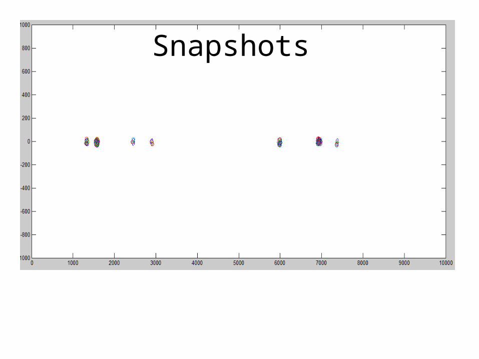
Snapshots

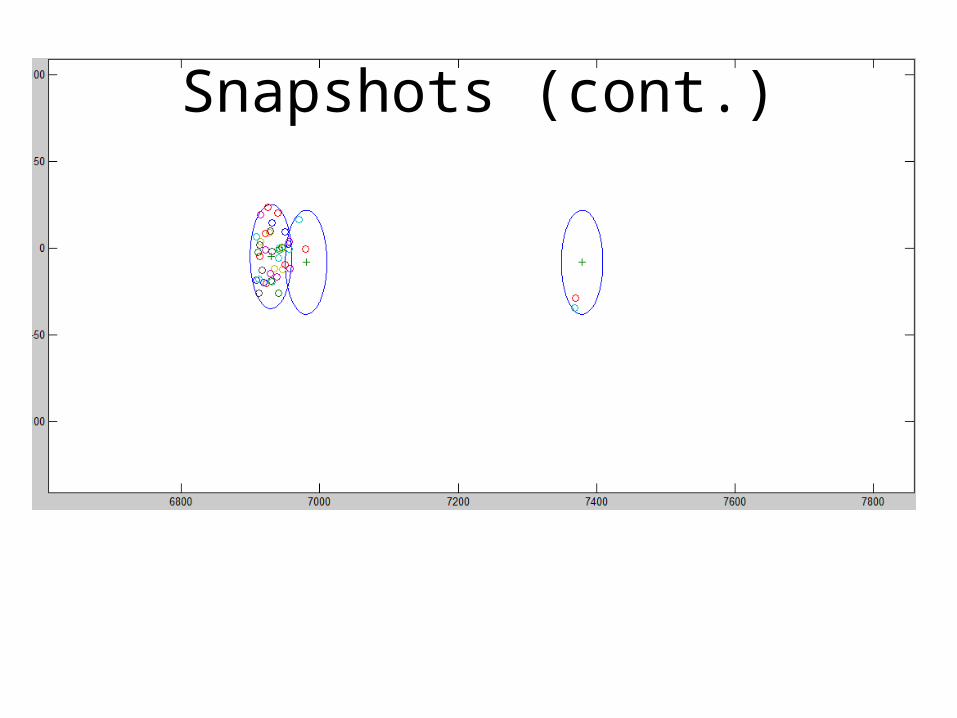
Snapshots (cont.)

DYNAMIC CLUSTERING ALGORITHMContinuous Clustering of Moving Objects.

• In this work, a dynamic clustering algorithm is used to cluster the cell phones generated from the previous step.

• The cluster behavior can then be estimated and used as a vehicle behavior (under the

assumption : a cluster of cell phones is a moving vehicle).

How We Cluster

• This clustering algorithm utilizes the cellphones location and speed at each time step to predict the cellphones positions in the near feature.

• This method makes sure that in the near future cellphones will remain part of their clusters. In-addition, cluster split/merge actions can be predicted.

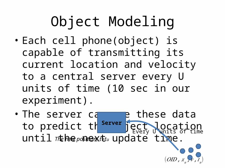
Object Modeling• Each cell phone(object) is capable of

transmitting its current location and velocity to a central server every U units of time (10 sec in our experiment).

• The server can use these data to predict the object location until the next update time.

Server

(𝑂𝐼𝐷 , 𝑥𝑢 ,𝑣 ,𝑡𝑢)

Every U units of timeThe new position, t>tu

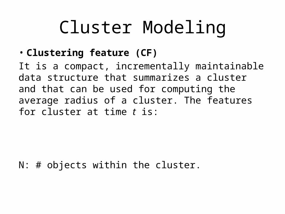
Cluster Modeling• Clustering feature (CF) It is a compact, incrementally maintainable data structure that summarizes a cluster and that can be used for computing the average radius of a cluster. The features for cluster at time t is:

N: # objects within the cluster.

CF Claims

• CF at time can be updated at new time based on its value at and .

• If object given by is inserted or deleted to acluser with CF it becomes

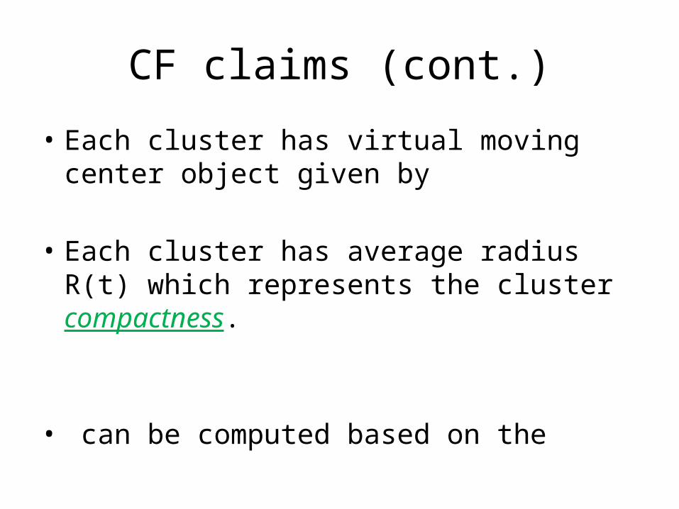
CF claims (cont.)

• Each cluster has virtual moving center object given by

• Each cluster has average radius R(t) which represents the cluster compactness.

• can be computed based on the

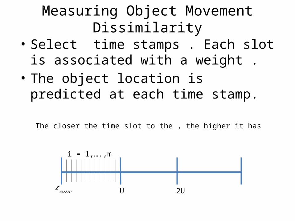
Measuring Object Movement Dissimilarity

• Select time stamps . Each slot is associated with a weight .

• The object location is predicted at each time stamp.

The closer the time slot to the , the higher it has

𝑡𝑛𝑜𝑤 U 2U

i = 1,….,m

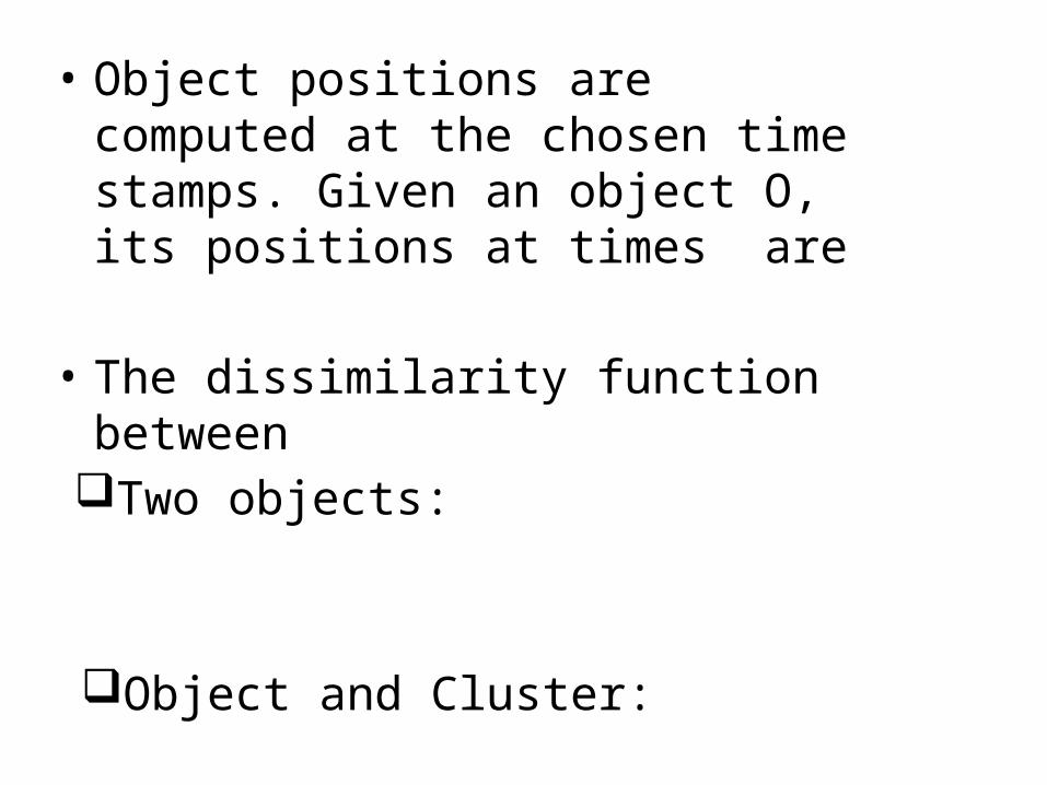
• Object positions are computed at the chosen time stamps. Given an object O, its positions at times are

• The dissimilarity function between Two objects:

Object and Cluster:

The Insertion Operation

• To insert object O with . Find the cluster C with the closest center to O, using M function.

• Introduce threshold represents the max acceptable distance between the closest clusters.

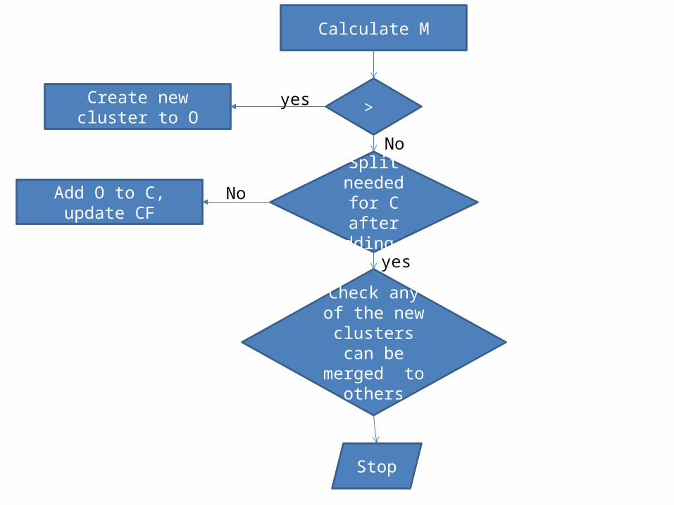
Calculate M

> Create new cluster to O

Split needed for C after adding O

Check any of the new clusters can

be merged to others

Stop

Add O to C, update CF

yes

yes

No

No

The Deletion Operation

• Next, to delete an object O, a hash table was used to locate the cluster C that object O belongs to. Then we remove object O, and we adjust the clustering feature for C.

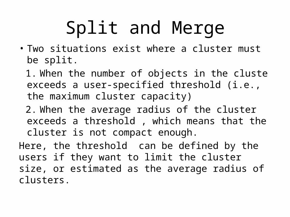
Split and Merge• Two situations exist where a cluster must be split.

1. When the number of objects in the cluste exceeds a user-specified threshold (i.e., the maximum cluster capacity) 2. When the average radius of the cluster exceeds a threshold , which means that the cluster is not compact enough.

Here, the threshold can be defined by the users if they want to limit the cluster size, or estimated as the average radius of clusters.

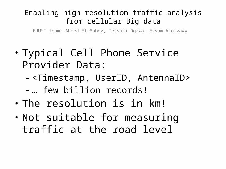
Enabling high resolution traffic analysis from cellular Big data

• Typical Cell Phone Service Provider Data:– <Timestamp, UserID, AntennaID>– … few billion records!

• The resolution is in km!• Not suitable for measuring traffic at the road

level

EJUST team: Ahmed El-Mahdy, Tetsuji Ogawa, Essam Algizawy

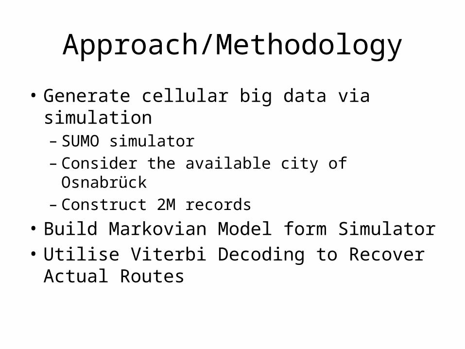
Approach/Methodology

• Generate cellular big data via simulation– SUMO simulator– Consider the available city of Osnabrück– Construct 2M records

• Build Markovian Model form Simulator• Utilise Viterbi Decoding to Recover Actual

Routes

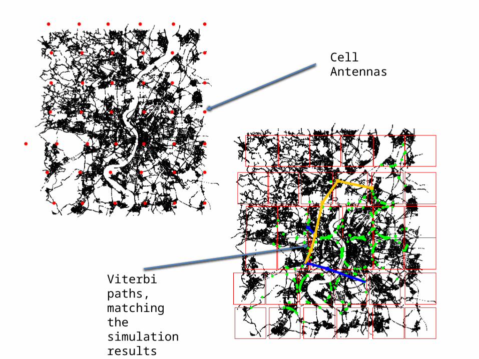
Viterbi paths, matching the simulation results

Cell Antennas

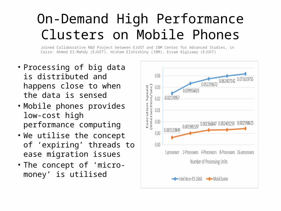
On-Demand High Performance Clusters on Mobile Phones

• Processing of big data is distributed and happens close to when the data is sensed

• Mobile phones provides low-cost high performance computing

• We utilise the concept of ‘expiring’ threads to ease migration issues

• The concept of ‘micro-money’ is utilised

Joined Collaborative R&D Project between EJUST and IBM Center for Advanced Studies, in Cairo: Ahmed El-Mahdy (EJUST), Hisham Elshishiny (IBM), Essam Algizawy (EJUST)

Thank you