Dowry:

Household Responses to Expected Marriage Payments

S Anukriti∗ Sungoh Kwon† Nishith Prakash‡

First draft: October 2016 §

Abstract

Dowry is a ubiquitous feature of South Asian marriage markets. However, empirical researchon dowry has been limited by the lack of data. We utilize retrospective information on giftsexchanged at the time of marriage for 39,544 marriages during 1960-2008 to describe dowrytrends in contemporary rural India. Average real net dowry has been remarkably stable over time;although there is considerable heterogeneity across castes, religions, and states. Additionally, weexamine the impact of dowry expectations on households’ financial and childbearing decisionsand on investments in children. Parents increase savings and fathers work more in anticipationof future marriage payments for their daughters. However, dowry has no impact on fertility andsex-selection. The effects on expenditure on children’s education are inconclusive.

JEL Codes: J12, J16, D10

Keywords: Dowry, Marriage, India, Savings, Education, Fertility, Sex Ratio, Employment

∗Department of Economics, Boston College. anukriti@bc.edu.†Department of Economics, University of Connecticut. sungoh.kwon@uconn.edu.‡Department of Economics & Human Rights Institute, University of Connecticut, IZA, HiCN, & CReAM.

nishith.prakash@uconn.edu.§We thank Prashant Bharadwaj, Mausumi Das, Anusar Farooqui, Delia Furtado, Parikshit Ghosh, Rachel Heath,

Rob Jensen, Adriana Kugler, Hyun Lee, Annemie Maertens, Subha Mani, J.V. Meenakshi, Laura Schechter, ChrisUdry, Shing-Yi Wang, David Weil, and participants at various seminars and conferences for their helpful commentsand suggestions.

1 IntroductionMarriage matters a great deal for individuals’ well-being everywhere, but especially in countries,such as India, where it is nearly universal. Historically, marriage has been an arranged, economicagreement between the bride, the groom, and their families, and it continues to be so in manycontemporary societies.1 A key feature of these marriages is bride-to-groom (dowry) or groom-to-bride (bride price) payments at the time of marriage. These marriage payments are widelyprevalent in several developing countries and can be large enough to affect the welfare of householdsand a society’s distribution of wealth. Like any custom or cultural norm, in the very long-run,societies have witnessed complete disappearance of marriage payments (e.g., in Europe) as well astransformations from one type to another (e.g., in Bangladesh). Nevertheless, in most contexts, theexpected direction of marriage payments is quite stable over an individual’s lifetime, even if theexact amount is unknown prior to and is negotiable at the time of marriage. We seek to answerthe following question in this paper: how do families and individuals respond to these expectedmarriage payments?

We focus on dowry payments in contemporary India. Despite being illegal since 1961, dowryis almost universal in India and imposes a substantial burden on girls’ families at the time ofmarriage, often amounting to several years of household income. Although birth of a child imposessome costs on parents in any context, dowry imposes an additional shock—that differs by genderof the child—to parents’ expected future income. After the child gender is realized, parents of a sonexperience an increase in their expected permanent income, while those of a daughter experience adecline. We examine the effect of this shock on parents’ current financial and childbearing decisionsand on child investments after the birth of a girl versus a boy.

Theoretically, the effect of expected future dowry payments on savings, labor supply, and childinvestments is ambiguous. In an inter-temporal utility maximization framework, new informationabout future income should lead to immediate adjustments in the optimal consumption path.An increase in expected permanent income (in boy families) should cause an increase in currentconsumption. However, if households are credit constrained, they may be unable to borrow inanticipation of this income increase, and therefore consumption may only change at the time theincome increase materializes (i.e., upon marriage) and not in advance. For girl families, whenincome is expected to decline, households can still save more and lower consumption in advance.2

In addition, girl parents may work more relative to boy parents due to the income effect of thedowry shock or to smooth income if markets are incomplete. Again, the ability of boy parents toincrease current leisure may be muted by credit constraints.

Another channel that adds to the ambiguity is human capital investment (HCI). Direct HCI in

1In the 2012 Human Development Survey of India, only 5 percent of ever-married women aged 25-49 reportedthat they had a self-arranged or “love” marriage.

2The decrease in consumption may also take the form of lower investments in children’s human capital, especiallygirls’.

1

the daughter may act as a substitute for dowry on the marriage market if labor market returns tofemale education are sufficiently high or if a better educated bride is more valuable to the groom’sfamily (e.g., to raise higher quality children). Thus, for a given expected dowry amount, parents ofa daughter who foresee higher returns to female education (or health) on the marriage and labormarkets, may increase savings by a lesser amount and may instead invest more in the daughter’shuman capital, relative to parents who foresee lower returns to female HCI. Thus, our researchquestion is essentially an empirical one.

There are two major challenges to estimating the causal effect of expected dowry payments onoutcomes of interest in this literature. First is the likely endogeneity of the dowry variable. We defineexpected dowry as the average net dowry paid by brides or received by grooms from the same casteand state as the child and who married during the year of the child’s birth or the prior four years.While our dowry variable is pre-determined, it is not exogenous if it is correlated with unobservablesthat also affect the outcome variables. One way to address this concern is by utilizing the fact thatdowry affects parents of boys and girls in the opposite manner—the former expect to receive andthe latter expect to pay dowry upon marriage. The second issue arises because boy families and girlfamilies are likely to be different along other dimensions that are correlated with the outcomes. Thisis especially true as selective abortion of girls is widespread in contemporary India. To address thisconcern, we distinguish between households that differ by firstborn sex. Despite access to prenatalsex-determination technology, the sex ratio at first parity has remained unbiased in India and isfrequently used as an exogenous shock in related literature (?, ?, ?, ?). While parents of a firstborngirl (FG) may be more likely to have a subsequent birth and to sex-select due to a desire for atleast one son (or to compensate for the negative income shock due to a FG), they should still havemore girls on average than firstborn boy (FB) households.3 Therefore, the first child’s gender canbe reasonably considered an imperfectly anticipated permanent income shock at the time of birth.4

Thus, we estimate the causal impact of dowry expectations by interacting randomly determinedfirstborn sex with pre-determined expected dowry payments.

We implement this empirical strategy by using the 2006 Rural Economic and DemographicSurvey (REDS) of India. This dataset contains several questions that are not commonly askedin most Indian household surveys. First, unlike other Indian datasets that record total marriageexpenditure by families similar to the respondent’s family, REDS reports actual payments bybrides and grooms in the surveyed households. Using retrospective information on gifts given andreceived at the time of marriage, we compute the net real payment by the bride (“dowry”) for39,544 marriages that took place during 1960-2008. Second, REDS collects rich information onvarious forms of savings at the household level.5

Our main findings are as follows. First, we document the trends in dowry payments in India

3This would not be the case if FB parents abort subsequent male fetuses in order to have a daughter. However,there is no empirical evidence to support this claim.

4The income shock will however be anticipated at the time of child’s marriage.5For example, savings in financial institutions, in jewelry, in livestock, and in durable goods.

2

and find that average dowry has been remarkably stable over time, albeit there is considerableheterogeneity across castes, religions, and states. Second, as expected dowry increases, FG familiessignificantly increase per capita savings overall and relative to FB families. There is no significantchange in FB households’ savings when they expect to receive higher dowry implying the presenceof credit constraints. Interestingly, FG families increase formal savings in financial institutions anddo not invest more in jewelry or precious metals that are traditionally considered an integral part ofdowry in India. Third, FG fathers work more days in a year relative to FB fathers as expected dowryburden goes up. However, dowry does not seem to be a significant explanatory factor for differentialfertility and sex-selection in FG and FB families. Lastly, the impact of dowry expectations on childinvestments is unclear. On the whole, we find that the custom of dowry significantly alters thefinancial decisions of a household, and parents respond in a manner that suggests that daughterscontinue to be considered an economic liability in India.

Our results contribute to several literatures. While dowries have received considerable attentionin the economics literature, a lot of it is theoretical (e.g., ?, ?, ?). While dowry trends in India havebeen the subject of a lively debate (?, ?), the empirical arguments have relied upon a small samplecollected by the International Crops Research Institute for the Semi-Arid Tropics (ICRISAT) thatis not nationally representative and is outdated (?, ?, ?).6 Other recent papers that study dowryin India using alternate data (e.g., ?, ?, ?, ?) do not analyze dowry trends. As such, our firstcontribution is that we describe the evolution of and the heterogeneity in dowry by caste, religion,and state in contemporary India.

Second, we contribute to the growing body of work on the effects of marriage payments.7 Weare not aware of any study that estimates the causal impact of dowry on household savings, laborsupply, and expenditure on children’s education. While ? and ? have examined, using ICRISATdata, the association between female birth, savings, and parents’ time allocation in India, they donot use dowry data and thus do not explicitly show that dowry is the underlying mechanism fortheir findings. Moreover, their analyses are less relevant for post-1980 India where sex-selection hasmade child gender endogenous. Our analyses of fertility and sex-selection are related to ? and ?,but our results differ.

We also make a modest contribution to the large literature on income and consumption smooth-ing (?). Our finding that households use savings and adjust labor supply to smooth negative incomeshocks is consistent with classical life-cycle and permanent income models (?, ?, ?). The lack ofsmoothing in response to positive income shocks is also consistent with the empirical literature onliquidity or credit constraints (?). Lastly, our work is tangentially related to the research on theimpact of sex ratios on savings (?, ?).

The rest of the paper is organized as follows. Section 2 describes the data, while Section 3discusses dowry trends in contemporary India. Section 4 presents the empirical strategy. The main

6More details are in Section 3.7See ? for brideprice and ?, ?, and ? for dowry.

3

results are discussed in Section 5. Section 6 presents a variety of robustness checks and Section 7concludes.

2 DataWe use the most recent 2006 round of REDS, which is a nationally representative survey of ru-ral Indian households first carried out in 1968. In addition to detailed information on savings,labor supply, and other economic and demographic variables, REDS includes retrospective ques-tions on marriage histories of household members.8 Unlike other datasets, e.g., the Indian HumanDevelopment Survey (IHDS), that record total marriage expenditure by families similar to therespondent’s family as reported in the year of survey, REDS collects data on actual payments bybrides and grooms in the surveyed households. Specifically, it reports the value of gifts received orgiven at the time of marriage in addition to the year of marriage and demographic information ofspouses (e.g., caste, age, and years of schooling).

Our primary outcomes of interest are different measures of saving, father’s days worked, andexpenditure on children’s education. Using the detailed information available in REDS, we constructthe following measures of household saving in per capita terms: total savings, formal savings, savingsin jewelry, savings in livestock, and savings in durable goods.9 The saving variables are constructedbased on the value of each item purchased (deposits) and sold (withdrawals) during 2005-06, i.e.,we only have information on savings at one point in time. The employment history in REDS 2006,however, provides the number of days worked each year between 1982 and 2006, which we use toconstruct a panel data set of fathers’ labor supply.10

Table 1 provides summary statistics of the key variables used in our analysis. An averagehousehold expects to pay or receive Rs. 26,420 as dowry. Educational attainment is low—the yearsof schooling for an average father and mother are, respectively, 6 and 4. OBCs are the largest castegroup in the sample (47 percent), followed by other “upper” castes (27 percent), SCs (18 percent),and STs (8 percent). In terms of religion, Hindus are the majority (88 percent). The mean numberof children at the time of survey is 2.09. The year of birth for firstborn child ranges from 1992to 2008. We restrict the child age to less than 15 before constructing birth order. We restrict oursample to nuclear households since savings data in REDS are available only at the household level.

3 Dowry in Contemporary Rural IndiaThe first objective of this paper is to document the trends in dowry payments in contemporaryrural India. There has been a lively debate in the literature on whether India (and the rest ofSouth Asia) has been experiencing dowry inflation, and, if so, whether it has been caused by an

8The 2006 REDS collected marriage histories of a household head’s sons, daughters, brothers, sisters, and nonco-resident parents.

9A detailed description of variable definitions is available in Section 8.10During the year of REDS survey in 2006, about 95 percent of fathers in the data set reported their primary activity

to be: self-employed farming, self-employed non-farming, salaried work, agricultural wage labor, or non-agriculturalwage labor.

4

excess supply of women on the marriage market, referred to as the “marriage squeeze” (e.g., ?, ?,?).11 Remarkably, this debate has been based on data from an extremely small sample that is notnationally representative. The International Crops Research Institute for the Semi-Arid Tropics(ICRISAT) sample used in ? and ? comprises 141 households from six villages in three districts ofrural South Central India collected in 1983 through a retrospective survey on marriage.12 This islikely due to lack of data on dowries during the time period examined by these studies, roughly 1923-1978. Other papers on this topic (e.g., ?) have been theoretical and have assumed the presence ofdowry inflation and have sought to test if marriage squeeze is a credible explanation for it. Moreover,these studies do not inform us about trends in more recent years that have witnessed remarkableeconomic and social changes.

Recently, ? use data from Bangladesh, India, Nepal, and Pakistan to assess this prior research,and conclude that there is no dowry inflation in South Asia. For India, in addition to the 1983ICRISAT survey used by the aforementioned studies, they use the Survey of Women and theFamily (SWAF) conducted in 1993-94. While SWAF data is more recent than ICRISAT data, a keyshortcoming of it, that the authors acknowledge, is that it does not report specific dowry amountsand instead provides five ordinal categories that nominal dowries fall into.

We supplement this literature by utilizing another data source—REDS 2006—that is morerecent, is larger, is more representative, and provides retrospective information on the nominalvalue of gifts received or given at the time of marriage for each year during 1960 and 2009. Whilesome recent papers have used this dowry data (?, ?, ?) for part of their analyses, none have usedit to describe the cross-sectional and temporal variation in dowries.

In this section, we describe the evolution of (i) gross payments by the bride’s family to thegroom or his family, (ii) gross payments by the groom’s family to the bride’s family, and (iii) netdowry computed as the difference between (i) and (ii). We deflate the nominal amounts using the2005 Consumer Price Index (CPI) and plot 5-year moving averages in most graphs.

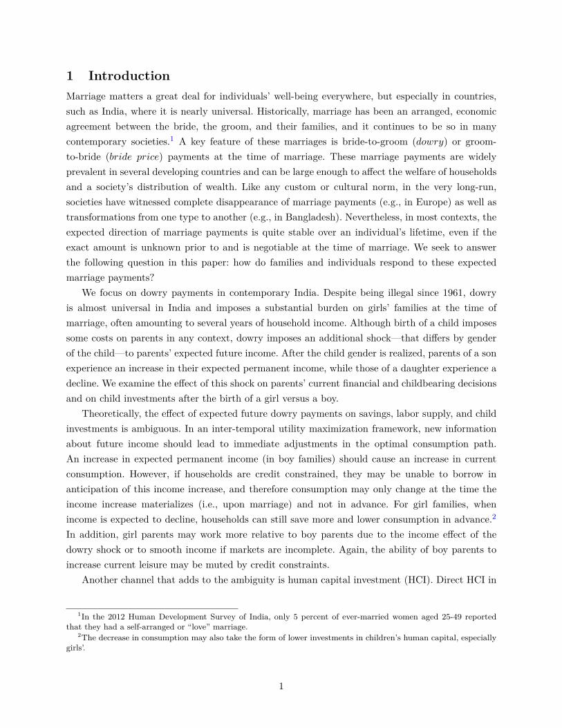
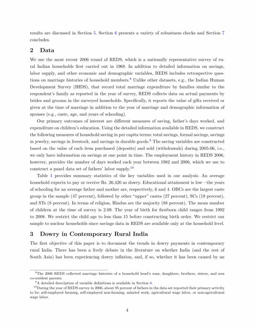
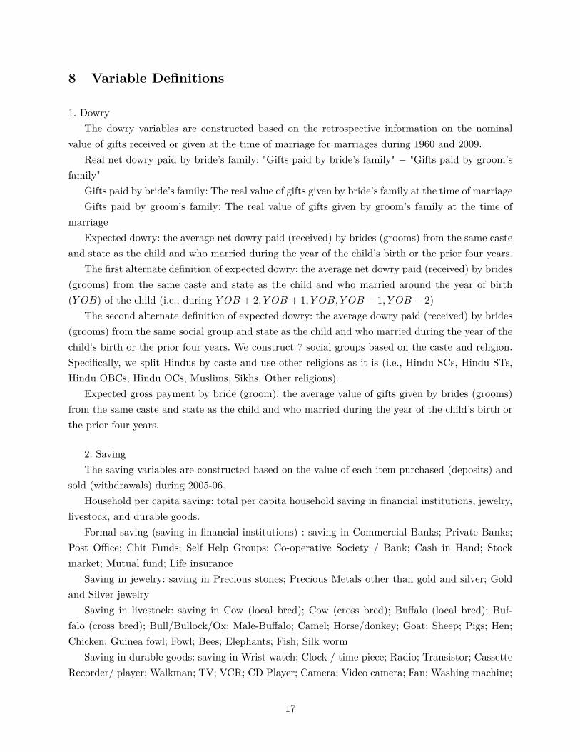
Figure 1 shows that average dowry has been remarkably stable over time, with some dowryinflation during 1960-73 and 2000-09. The trend in net dowry is mimicked by the trend in grosspayments by the bride’s family to the groom’s family. The flow of payments in the opposite direction,i.e., from the groom to the bride, is also positive throughout, but substantially smaller. While anaverage groom’s family spends about INR 5,000 on gifts to the bride’s family, gifts from the bride’sfamily cost seven times more, i.e., about INR 35,000. Thus, the real net dowry fluctuates aroundINR 27,000 during 1973-1995 in our sample.13 As per capita incomes have risen in India during ourstudy period, these stable trends imply that, on average, dowry as a share of household income has

11? provide a detailed and comprehensive discussion of this debate.12The six ICRISAT villages belong to two states: Andhra Pradesh (Aurepalle and Dokur villages of Mahbubnagar

district) and Maharashtra (Shirapur and Kalman under Solapur district, Kanzara and Kinkhed under Akola district).The total number of surveyed households was 240, but the regression analysis sample in ? and ? comprises 141 and160 households, respectively, due to missing data.

13The INR 27,000 amount is roughly similar to the dowries reported in Figure 1 of ? during 1923-78.

5

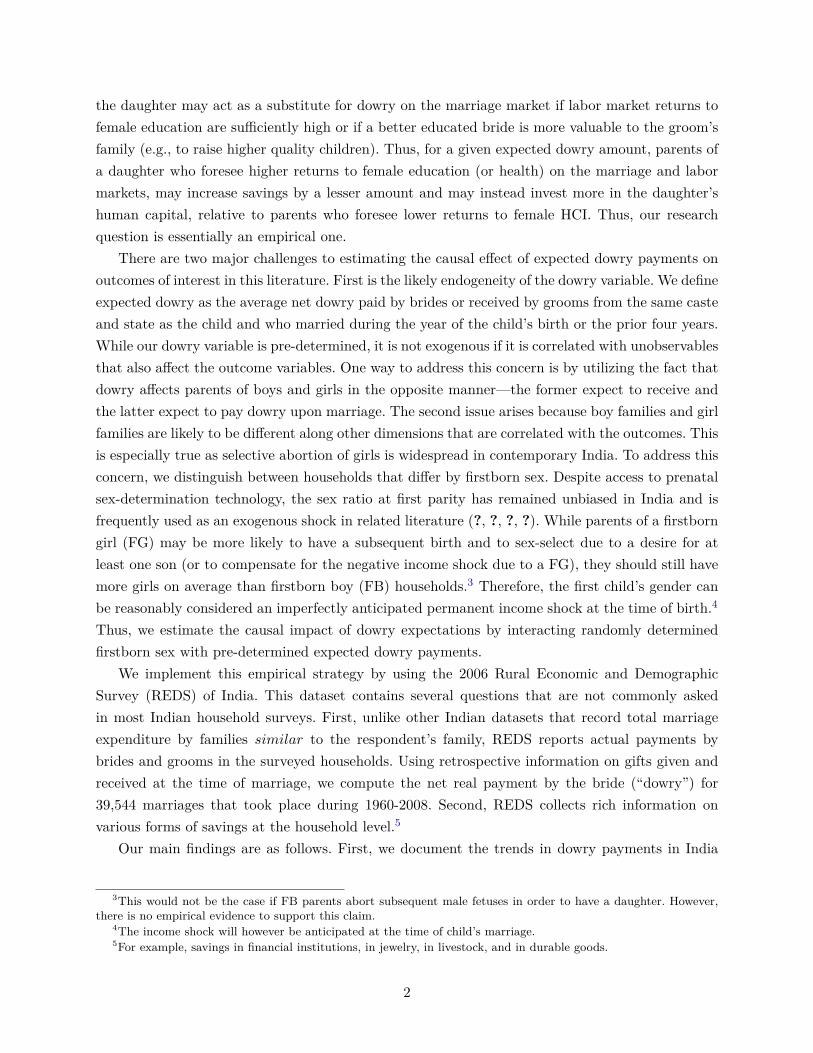
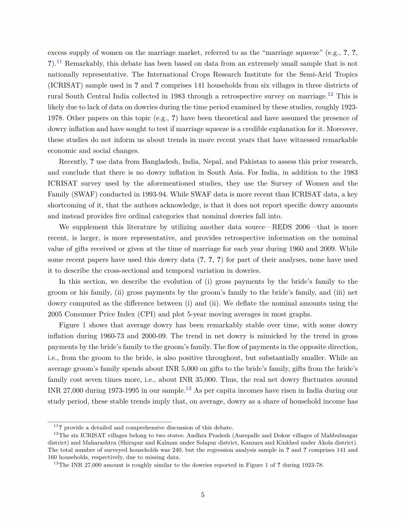
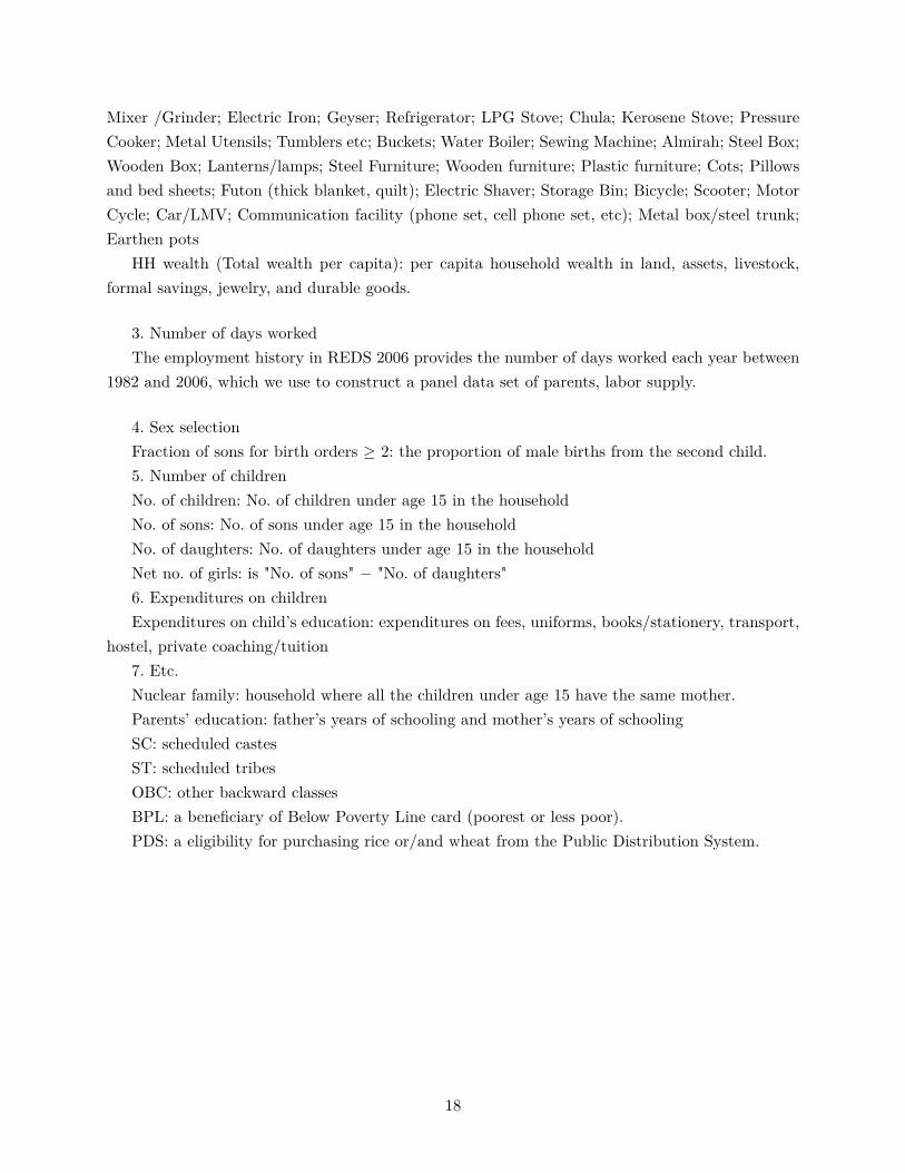
gradually declined at the national level. Figure 2 plots the distribution of net and gross marriagepayments. The proportion of marriages with a negative net dowry, i.e., where the groom’s familypaid more to the bride’s family than the other way around, is non-zero, but quite small. The vastmajority of the marriages involved positive net dowry payments to the groom’s family. We do notobserve any marriages where the value of gifts was reported to be zero.14

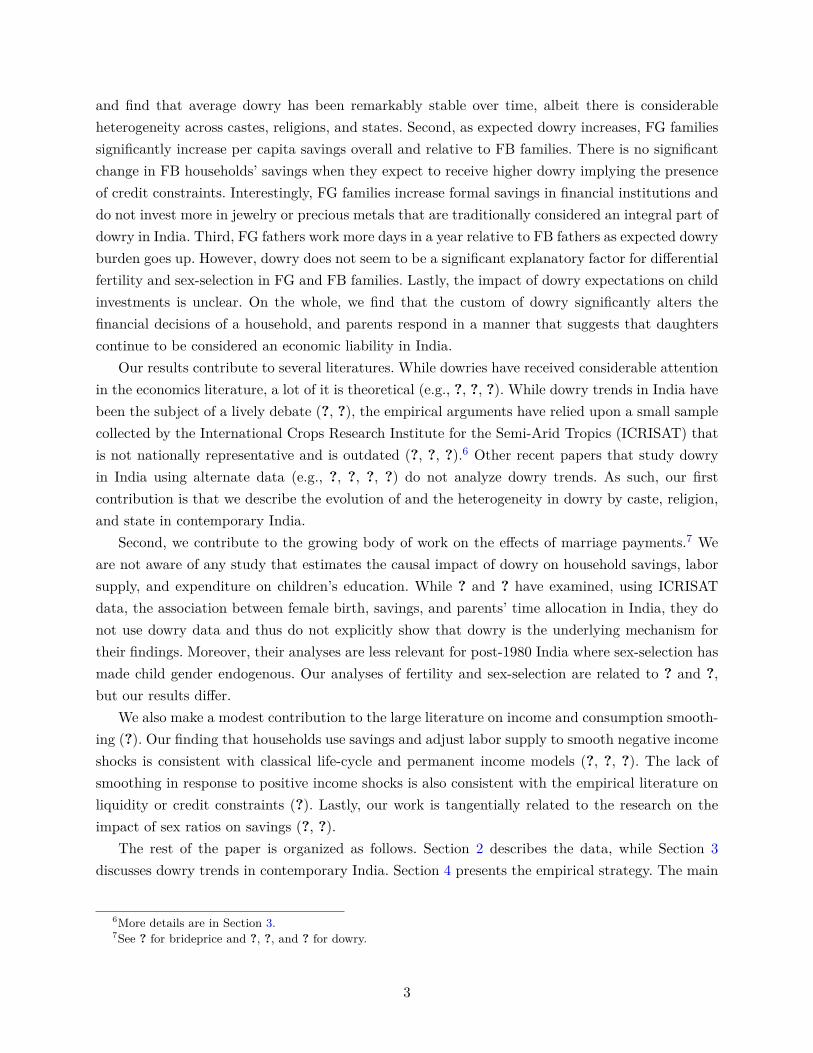
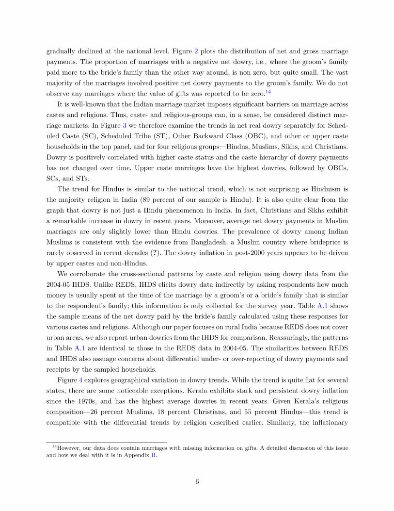
It is well-known that the Indian marriage market imposes significant barriers on marriage acrosscastes and religions. Thus, caste- and religious-groups can, in a sense, be considered distinct mar-riage markets. In Figure 3 we therefore examine the trends in net real dowry separately for Sched-uled Caste (SC), Scheduled Tribe (ST), Other Backward Class (OBC), and other or upper castehouseholds in the top panel, and for four religious groups—Hindus, Muslims, Sikhs, and Christians.Dowry is positively correlated with higher caste status and the caste hierarchy of dowry paymentshas not changed over time. Upper caste marriages have the highest dowries, followed by OBCs,SCs, and STs.

The trend for Hindus is similar to the national trend, which is not surprising as Hinduism isthe majority religion in India (89 percent of our sample is Hindu). It is also quite clear from thegraph that dowry is not just a Hindu phenomenon in India. In fact, Christians and Sikhs exhibita remarkable increase in dowry in recent years. Moreover, average net dowry payments in Muslimmarriages are only slightly lower than Hindu dowries. The prevalence of dowry among IndianMuslims is consistent with the evidence from Bangladesh, a Muslim country where brideprice israrely observed in recent decades (?). The dowry inflation in post-2000 years appears to be drivenby upper castes and non-Hindus.

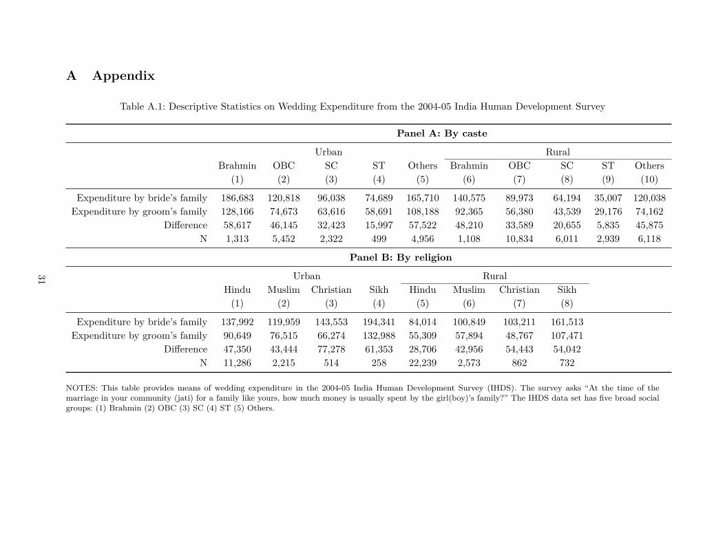
We corroborate the cross-sectional patterns by caste and religion using dowry data from the2004-05 IHDS. Unlike REDS, IHDS elicits dowry data indirectly by asking respondents how muchmoney is usually spent at the time of the marriage by a groom’s or a bride’s family that is similarto the respondent’s family; this information is only collected for the survey year. Table A.1 showsthe sample means of the net dowry paid by the bride’s family calculated using these responses forvarious castes and religions. Although our paper focuses on rural India because REDS does not coverurban areas, we also report urban dowries from the IHDS for comparison. Reassuringly, the patternsin Table A.1 are identical to those in the REDS data in 2004-05. The similarities between REDSand IHDS also assuage concerns about differential under- or over-reporting of dowry payments andreceipts by the sampled households.

Figure 4 explores geographical variation in dowry trends. While the trend is quite flat for severalstates, there are some noticeable exceptions. Kerala exhibits stark and persistent dowry inflationsince the 1970s, and has the highest average dowries in recent years. Given Kerala’s religiouscomposition—26 percent Muslims, 18 percent Christians, and 55 percent Hindus—this trend iscompatible with the differential trends by religion described earlier. Similarly, the inflationary

14However, our data does contain marriages with missing information on gifts. A detailed discussion of this issueand how we deal with it is in Appendix B.

6

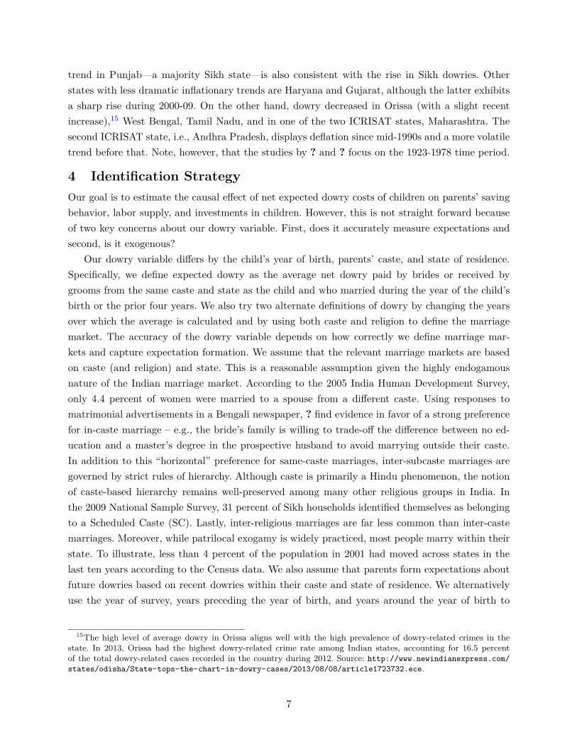
trend in Punjab—a majority Sikh state—is also consistent with the rise in Sikh dowries. Otherstates with less dramatic inflationary trends are Haryana and Gujarat, although the latter exhibitsa sharp rise during 2000-09. On the other hand, dowry decreased in Orissa (with a slight recentincrease),15 West Bengal, Tamil Nadu, and in one of the two ICRISAT states, Maharashtra. Thesecond ICRISAT state, i.e., Andhra Pradesh, displays deflation since mid-1990s and a more volatiletrend before that. Note, however, that the studies by ? and ? focus on the 1923-1978 time period.

4 Identification StrategyOur goal is to estimate the causal effect of net expected dowry costs of children on parents’ savingbehavior, labor supply, and investments in children. However, this is not straight forward becauseof two key concerns about our dowry variable. First, does it accurately measure expectations andsecond, is it exogenous?

Our dowry variable differs by the child’s year of birth, parents’ caste, and state of residence.Specifically, we define expected dowry as the average net dowry paid by brides or received bygrooms from the same caste and state as the child and who married during the year of the child’sbirth or the prior four years. We also try two alternate definitions of dowry by changing the yearsover which the average is calculated and by using both caste and religion to define the marriagemarket. The accuracy of the dowry variable depends on how correctly we define marriage mar-kets and capture expectation formation. We assume that the relevant marriage markets are basedon caste (and religion) and state. This is a reasonable assumption given the highly endogamousnature of the Indian marriage market. According to the 2005 India Human Development Survey,only 4.4 percent of women were married to a spouse from a different caste. Using responses tomatrimonial advertisements in a Bengali newspaper, ? find evidence in favor of a strong preferencefor in-caste marriage – e.g., the bride’s family is willing to trade-off the difference between no ed-ucation and a master’s degree in the prospective husband to avoid marrying outside their caste.In addition to this “horizontal” preference for same-caste marriages, inter-subcaste marriages aregoverned by strict rules of hierarchy. Although caste is primarily a Hindu phenomenon, the notionof caste-based hierarchy remains well-preserved among many other religious groups in India. Inthe 2009 National Sample Survey, 31 percent of Sikh households identified themselves as belongingto a Scheduled Caste (SC). Lastly, inter-religious marriages are far less common than inter-castemarriages. Moreover, while patrilocal exogamy is widely practiced, most people marry within theirstate. To illustrate, less than 4 percent of the population in 2001 had moved across states in thelast ten years according to the Census data. We also assume that parents form expectations aboutfuture dowries based on recent dowries within their caste and state of residence. We alternativelyuse the year of survey, years preceding the year of birth, and years around the year of birth to

15The high level of average dowry in Orissa aligns well with the high prevalence of dowry-related crimes in thestate. In 2013, Orissa had the highest dowry-related crime rate among Indian states, accounting for 16.5 percentof the total dowry-related cases recorded in the country during 2012. Source: http://www.newindianexpress.com/states/odisha/State-tops-the-chart-in-dowry-cases/2013/08/08/article1723732.ece.

7

define average expected dowry.As mentioned in the introduction, we utilize the fact that dowry affects parents of boys and

girls in the opposite manner—the former expect to receive and the latter expect to pay dowry uponmarriage. However, fertility and child composition may be endogenous. Before sex-selection waspossible, girls were born in relatively larger families as compared to boys, and larger family sizewould mechanically have lower savings per capita, irrespective of dowry expectations. Moreover, ifson-biased stopping rules or sex-selective abortions are more prevalent among groups with certainsocioeconomic characteristics that are also correlated with savings, for example, we are also likelyto encounter the omitted variables bias. Therefore, interacting expected dowry with the number orthe sex ratio of children is also not ideal.

In order to address the endogeneity, we interact expected dowry with firstborn sex. Despiteaccess to sex-selection, the sex ratio at first parity has remained unbiased in India and is frequentlyused as an exogenous shock in related literature (?, ?, ?). Table 1 provides summary statisticsof the key variables used in our analysis by the gender of the first child. Reassuringly, there areno significant differences between FB and FG families in terms of socioeconomic characteristicssuch as expected dowry, caste, religion, mother’s years of schooling, except for small differences infather’s schooling and belonging to a SC. Nevertheless, we control for all these covariates in ourspecifications. For given expected dowry per marriage, we expect FG families to save more that FBfamilies.

Ideally, we would focus on households that recently had their first child and compare FB familieswith FG families. However, due to sample size concerns, we first use the entire sample regardlessof the number and the composition of children. While FG parents may be more likely to have asubsequent birth and sex-select due to son preference or to compensate for the negative incomeshock from the first birth, FG families should still have more girls on average (unless parents of thefirst boy want to have a girl and abort male fetuses, which is unlikely), and hence we expect themto save more relative to FB families. Later, we examine heterogeneity in our results by the numberof children.

4.1 Savings

To investigate whether FG parents save more than FB parents during the survey year (2005-06)due to expected future dowry payment, we estimate the following specification for household i fromcaste c in state s and whose first child was born in year t:

Saving2005−06icst = α+ β1FirstGirli ×Dowrycst + β2Dowrycst + β3FirstGirli

+ πst + φct + ψsc + ηcFirstGirli + ηsFirstGirli + ηtFirstGirli

+ ωc + δs + θt + X′iγ + εicst,

(1)

where Saving2005−06icst denotes various measures of household saving in 2005-06; FirstGirli indicates

that the firstborn child in household i is female; Dowrycst is expected dowry defined as the averagedowry paid by brides from caste c in state s who were married during the year of the child’s birth

8

or the prior four years (i.e., during t, t− 1, t− 2, t− 3, t− 4);16 Xi is a vector of covariates compris-ing parents’ years of schooling, indicators for religion, and in some specifications, the household’snumber of children and wealth per capita.17 We report unweighted regressions in the main set oftables. However, our results remain the same when we use weights.18 Standard errors are clusteredat the state level. We also compute standard errors that are wild-cluster bootstrapped by state;these results are presented as robustness checks later.

The coefficient β2 captures how savings in FB families respond to expected dowry, while β1

captures the differential response of FG families to expected dowry, relative to the response ofFB families. The coefficient β3 describes the difference between savings behavior of FB and FGfamilies when expected dowry is zero. Thus, the inclusion of the FG main effect allows us tocontrol for any changes in per capita saving that could result for factors unrelated to dowry, forinstance, higher fertility among FG families due to the desire for at least one son. To exclude otherconfounding factors related to the caste, state, gender, and year of birth of the firstborn child,we control for all main and interaction fixed effects for these factors (i.e., ωc, δs, θt, πst, φct, ψsc,ηcFirstGirli, ηsFirstGirli, ηtFirstGirli).

Thus, any remaining threats to identification come from caste-state-year specific factors thatmay be correlated with Dowrycst and that differentially affect FG and FB parents. If this is so, thecoefficient of interest, β1, would then be contaminated by these omitted variables, and would notcapture the causal effect of dowry expectations. One such factor could be fertility. If dowry changesin a caste-state-year are correlated with changes in, say, the degree of son preference, the likelihoodand the sex ratio of higher parity births may differ by firstborn sex. Additionally, if dowry is moreprevalent in regions with stronger son preference, we would expect FG families to be more likely tohave subsequent births if they are following son-biased stopping rules with or without sex-selection,and that is likely to lower per capita savings. Therefore this bias would go against us. A higher sexratio may eventually also reduce dowry due to scarcity of women on the marriage market (althoughthere is currently no evidence that this has happened in India). However (1) our variable of interestis expected dowry, which is what determines parents’ financial decisions when the child is youngand (2) a lower expected dowry should make parents less likely to save.

Fertility could also be directly affected by expected dowry if FG families respond to dowryexpectations by increasing sex-selection for subsequent births (to have a compensating son whowould receive dowry), that could lower fertility (and household size), and thereby increase per

16The robustness checks using alternate definition of dowry expectation are provided in Section 7.17Instead of including religion fixed effects, we also try an alternate definition of marriage markets based on caste

and religion, along with state and year. These results are described later as a robustness check.18The 2006 REDS data does not provide sampling weights, hence we construct them in the following manner. Using

the village listing data which includes all households in REDS villages, we create an indicator for the householdsthat are actually sampled and regress it on the observables in the listing data. These inverted predicted probabilitiesserve as weights, assuming that the observables capture differential reasons for being surveyed. The observables inthe listing sheet data used to construct weight are household size, number of earners in the household, head’s age,head’s years of schooling, indicators of head’s caste (SC, ST, OBC, OC), religion (Muslim), and gender, and statefixed effects.

9

capita savings. To test if this the case, we re-estimate equation (1) by using fertility and theproportion of sons in second and higher parity births as the dependent variables. We also directlyinclude fertility as a control when we estimate the effect on savings using specification (1).

Lastly, we examine how our results change when we restrict the sample to households withspecific number of children. A strict test for our story comes from one-child families. Since thesefamilies have not yet had a second child, any saving response to firstborn sex and expected dowrycannot be due to endogenous fertility change. Restricting to a short time horizon after the birthof the first child is good as it shuts down the re-optimization that takes place in response to therevelation of the first child’s gender.

4.2 Labor Supply

The birth of a son or a daughter can affect parents’ time allocation in the following ways. Thepermanent income shock is a pure lottery and doesn’t change the reward or wage from working,i.e., there is no substitution effect. However, the income effect implies that in the absence of creditconstraints, FB parents should increase leisure, i.e., decrease labor supply and FG parents shouldincrease labor supply. When the household is credit constrained, the inability to borrow impliesthat current leisure may not increase, i.e., current labor may not decrease, when permanent incomegoes up for FB parents.19

Using the employment history between 1982 and 2006, we estimate the labor supply responsefor individual i from caste c in state s in year t′ and whose first child was born in year t. Thefollowing specification estimates the impact on labor supply:

Lit′ = α+ β1FirstGirli × Postt′>t ×Dowrycst

+ β2Postt′>t ×Dowrycst + β3FirstGirli × Postt′>t

+ δst′ + θct′ + πtt′ + γi + ωt′ + εit′ ,

(2)

where Lit′ are the the number of days worked in year t′; Postt′>t equals 1 if t′ > t, and 0 otherwise;and FirstGirli and Dowrycst are defined as before. We include the time interaction fixed effects(i.e., δst′ , θct′ , πtt′) as well as time fixed effects (ωt′) in this specification. The coefficient β2 captureshow expected dowry affects parents’ number of days worked after the birth of a firstborn boy andβ1 captures the differential response of parents of a firstborn girl after her birth. The panel natureof the labor supply variable allows us to control for individual fixed effects (γi). To test if father’s

19The predictions for mothers are not as straightforward. While child rearing may involve some decline in marketwork irrespective of child gender, returns to investment of women’s time in child-care on the marriage market maybe an additional consideration while allocating time. If sons with higher HKI obtain higher dowry, FB mothers maydecrease labor supply even more, if there are no credit constraints. Similarly, if daughters with higher HKI pay smallerdowries, FG mothers may also work less outside the home to invest in daughters’ HKI; however, in that case FGfathers would work even more to compensate for the loss of mothers’ income. In any case, 89 percent of the mothersin our dataset report being a housewife as their primary occupation. Since the data does not report days workedseparately for primary and secondary occupations, we cannot credibly estimate the effect on market- and non-marketwork for mothers, and hence focus only on fathers.

10

response varies by measure of wealth, we estimate specification (2) by whether a household’s wealthper capita is below or above the median.

4.3 Children’s Education

Next we estimate the effect of dowry expectations on investments in children’s education. For childi of birth-order b born in household j, caste c, in state s and year T and whose oldest sibling wasborn in year t we estimate the following specification separately for boys and girls:

Y b,gijcst =α+ β1Firstgirlj ×Dowrycst

+ β3Dowrycst + πst + φct + ψsc + ηcFirstgirlj + ηsFirstgirlj + ηtFirstgirlj

+ ρbt + β2Firstgirlj +Xjγ + ωc + δs + θt + κb + ψT + εicst

(3)

The dependent variable is the sum of expenditures on fees, uniforms, books or stationery,transport, hostel, and private coaching or tuition of a child.

5 Results5.1 Savings

In Table 2 we present results from equation (1) that estimates the impact of expected futuredowry payments on parents’ current saving behavior. Note that the expected dowry variable is inRs. 10,000. Our preferred specification is column (4). We add controls as we move from column(1) to column (5). We show how expected dowry differentially affects total household per capitaannual saving in FG and FB families. The coefficient of Firstborn girl is negative and not alwayssignificant, implying that, in the absence of dowry expectations, FG families do not save morethan FB families. However, when expected dowry is positive, FG families save significantly morethan FB families, and, within FG families, savings increase with the amount of expected dowry.FB families decrease savings when anticipated dowry receipts are higher, although the coefficientsare largely insignificant. These results suggest that while a negative permanent income shock dueto dowry expectations induces FG families to start saving more in advance, a positive permanentshock is not as effective for FB families. This potentially reflects the presence of credit constraintsdue to which FB families cannot borrow against the future dowry income and hence cannot increasecurrent consumption. The interaction coefficient in column (4) (= Rs. 532.94) translates into 57percent higher savings in FG families for a given expected dowry amount, relative to average annualsavings in FB families of Rs. 938. These findings are robust to the inclusion of household wealth asa control in column (5).

To address the endogeneity concerns related to differential fertility in FG and FB families, wefirst show that our results survive controlling for the number of children in column (5) of Table 2.Second, in Table 3, we re-estimate the effects on savings separately for families that have one child(in column 1), one or two children (in column 2), and one or two or three children (in column3). The sub-sample of one child families offer a strict test for our story since the saving behaviorof these families is has not yet been affected by the differential likelihood of higher parity births

11

or sex-selection of these births by firstborn sex. We find that families that have only a girl childalso save significantly more than families that have only a boy child. As we increase fertility of oursub-samples, note that while average per capita savings fall even for FB families (from Rs. 1380to Rs. 1068 to Rs. 971 in column (1)), we continue to see significantly higher savings among FGfamilies in each case. For given positive expected dowry, FG families in columns (1), (2), and (3)respectively save 92 percent, 62 percent, and 56 percent more than FB families’ average annualsavings.

The higher savings for FG families take the form of higher per capita formal saving in financialinstitutions (In Table 4). Contrary to conventional beliefs about dowries in India, we do not find asignificant difference in jewelry saving (in precious stones and metals) among FG and FB families.20

This pattern of saving behavior is consistent with greater access to financial institutions and instru-ments in rural India and the less liquid nature of jewelry relative to cash savings in bank accountsduring our study period. Similarly, there is no significant difference in terms of saving in livestock(although the coefficient is positive) and saving in durable goods. The interaction coefficient incolumn (1) (= Rs. 498) translates into 77 percent higher savings in FG families relative to averageper capita formal savings in FB families of Rs. 645.

?, on the other hand, find that an unexpected increase in the price of gold leads to immediaterise in fetal and infant mortality of girls, which suggests that families neither switch to alternateforms of dowry nor wait to realize if the price shock is permanent before withholding investments ingirls. If parents selectively eliminate daughters that become more expensive due to gold inflation,then the gold price shock, of course, does not have to translate into higher savings. However, bythat reasoning, FG families should also be more likely to practice sex-selection at higher parities asexpected dowry rises. However, we do not find this to be true in our data.21 Table 5 shows that FGfamilies have higher fertility and practice greater sex-selection even if expected dowry is zero, andthat there is no differential effect of dowry on future childbearing and sex-selection in FG familiesrelative to FB families. These findings not only assuage concerns about endogenous fertility, butare also important in their own right. It is frequently claimed that dowry is an underlying causeof son preference and discrimination against girls in India. While the desire for at least one son isreal and affects childbearing decisions, it leads to higher fertility and more male-biased sex ratioseven in the absence of dowry, and dowry does not seem to be an additional significant explanatoryfactor. In fact, our results also contradict the findings of ? who finds that an amendment that madethe Indian anti-dowry law stricter in 1985 led to decreases in male-biased fertility behaviors as itpotentially made the dowry cost of daughters smaller. Both ? and ? do not directly estimate theeffect of dowries on excess female child mortality, male-biased fertility, and the sex ratio at birth.

In Table 6 we provide further supporting evidence for the role of dowry in affecting savings

20This is true irrespective of whether the family has only one child, or ≤ two children, or ≤ three children.21We differ from ? in the other ways: they use data from the 1999 REDS, while we use the 2006 REDS. They define

dowry as the gross value of gifts from the bride’s side to the groom’s side, where as we use net dowry.

12

independently of its relationship with son preference. We restrict the sample to FB families. Sincethese parents already have a son, their desire to continue childbearing is less likely to be drivenby son preference and they are less likely to practice sex-selection than FG families. Within thissub-sample we then compare how expected dowry affects per capita savings across households thatdiffer in the net number of girls (defined as the number of girls minus the number of boys in afamily). Using net number of girls rather than total number of girls also allows us to shutdown anypotentially compensatory benefit of having an older brother whose dowry receipt may be used tofinance a younger sister’s dowry payment. The interaction coefficient continues to be positive andsignificant.

5.1.1 Heterogeneity

Next we test the role of income and credit constraints in the ability of parents to alter currentconsumption in response to changes in permanent income. Table 7 shows that the higher savingsfor FG relative to FB families for given positive expected dowry is driven by above median wealthhouseholds. The coefficient of Firstborn girl * Expected dowry is also positive for below median fam-ilies but is small and is insignificant, suggesting that income constraints limit poor parents’ abilityto save. For FB families, credit constraints would imply a smaller increase in current consumption(or decline in savings) for poorer households, which is what we find, but the coefficients of Expecteddowry are insignificant for both sub-samples.

In Appendix Table A.2 we also examine heterogeneity in the impact on savings by the edu-cational attainment of parents, by above versus below median expected dowry, and by residencein high versus low son preference state.22 While the interaction coefficient is positive across allsub-samples, it is significant only for high educated parents, above median dowry expectation, andhigh son preference states. This pattern of results is consistent with lower labor market returnsto HKI in daughters in high son preference states (that makes saving for dowry preferable overinvesting in girls’ education) and with greater dowry burden if expected dowry is above median.While it is unclear what to expect a priori in terms of heterogeneity by education, it is reassuringthat the coefficient size is larger for more educated families, as they presumable have higher incomeand thus can potentially save more for a given expected dowry than lesser educated families. Theeducation heterogeneity is consistent with the wealth heterogeneity in Table 7.

5.2 Father’s Labor Supply

The dowry shock causes FG fathers to work more relative to FB fathers; the latter do not exhibit asignificant change after the birth of their first child (column (1) in Table 8). The triple-interactioncoefficient translates into a 2.29 percent increase in FG fathers’ days worked relative to the averagedays worked by FB fathers (= 174). Note that, when expected dowry is zero, FG fathers do notwork more than FB fathers. These results are consistent with the income effect of future dowry

22High son preference states are Haryana, Punjab, Rajasthan, Uttar Pradesh, Madhya Pradesh, and HimachalPradesh

13

and the lack of decline in days worked of FB fathers implies that households are credit constrained.Columns (2) and (3) check if credit constraints are the reason why FB fathers cannot increaseleisure in advance of future income rise. To the extent that above median wealth households areless constrained than below median wealth households, the former should be more able to decreasework than the latter. Indeed the coefficient of Expected dowry * Post is negative for above medianwealth households, albeit insignificantly, but is positive for below median wealth families, implyingthat the income effect is somewhat stronger for less constrained families.

5.3 Children’s Education

As discussed in the introduction, if labor market returns to female education are sufficiently high orif a better educated bride is more valuable to the groom’s family, then bridal families may chooseto invest in daughters’ human capital directly. In addition, it is argued that bridal families aremindful of the fact that investing directly in their daughters improves their potential labor marketoutcomes and bargaining power within their marital household ?. Thus, for a given expected dowryamount, parents of a daughter who foresee higher returns to female education (or health) on themarriage and labor markets, may increase savings by a lesser amount and may instead invest morein the daughter’s human capital, relative to parents who foresee lower returns to female HCI.

We directly examine the effect of dowry on children’s education expenditure in Table 9. Wepresent the results for boys in columns (1) and (2) and for girls in columns (3) and (4). Resultsfrom a less strict specification (i.e., columns (1) and (3)) where we do not control for Firstborngirl∗Caste Fixed Effects, supports the claim that when expected dowry is positive, FG familiesinvest significantly more in daughters’ education expenditure while reducing the same for sons.However, in the stricter specification (i.e., columns (2) and (4)), we do not find the point estimatesto be statistically significant.

Given the little empirical research on the impact of marriage payments on HCI in children, withthe exception of ? who show that bride price provides a greater incentive for parents to invest ingirls’ education, we provide suggestive evidence that the effect of dowry on children’s educationexpenditure is statistically insignificant. Although inconclusive, our results contribute to the livelypublic debate on this topic over the plausible negative consequences of dowry payments in India.

6 Other Robustness ChecksWe perform a battery of additional robustness checks that include using two alternative defini-tions of expected dowry, replacing net dowry with two separate gross marriage payment variables,treatment of missing observations and outliers, and presenting the main results with wild-clusterbootstrapping. Our findings remain the same.

6.1 Alternate Definitions of Expected Dowry

We use two alternate definitions of expected dowry to test the sensitivity of our results. First,we reconstruct the expected dowry variable by incorporating both religion and caste in Table A.3.Specifically, we split Hindus by caste and use other religions as it is (i.e., our seven groups are: Hindu

14

SCs, Hindu STs, Hindu OBCs, Hindu OCs, Muslims, Sikhs, Other religions) and then separatelydefine expected dowry for these groups (while using state and year of birth as before).23 Second,instead of using the average of net dowries paid in marriages that occurred during the year of thechild’s birth (YOB) or the prior four years, in Table A.4 we use the average of net dowries paidaround the YOB of the child (i.e., during Y OB+ 2, Y OB+ 1, Y OB, Y OB− 1, Y OB− 2). In bothtables, our findings remain exactly the same as before.

6.2 Expected Gross Marriage Payments

Several economists have modeled dowry as net dowry following ?. Anthropologists, on the contrary,define dowry as the gross assets brought by the bride to the groom’s family at the time of marriage.? has argued that net dowry is likely to overstate the relative contribution of the bride’s family tothe groom’s family due to marriage market factors, especially among wealthier families, if dowriesalso comprise pre-mortem bequest to daughters. The only evidence on the relative importance ofthe bequest motive of dowries, that we are aware of, comes from ? who find that, in Bangladesh,bequest dowries have declined in prevalence and amount over time. Since the majority of Indianstates did not equalize inheritance rights between sons and daughters until as recently as 2005,bequest may, however, be a crucial component of Indian dowries during our sample period.

We check how replacing net dowry with its two component variables, i.e., gross payments bythe bride’s and the groom’s family in specification (1) alters the impact on savings. Since paymentsby the groom are several orders of magnitude smaller than those by the bride, we do not expectthis to matter. Table A.5 confirms our intuition. The coefficient of Firstborn girl * Expected grosspayment by bride continues to be positive and significant, albeit is slightly larger in magnitudethan the coefficient of Firstborn girl * Expected net dowry in Table 2. Moreover, the coefficient ofFirstborn girl * Expected gross payment by groom is always negative.

6.3 Wild-Cluster Bootstrap

Thus far we have clustered standard errors by state. However, given that the number of states (= 17)in our sample is relatively small, routine approaches to clustering may lead to underestimation ofstandard errors. To check if this is what underlies our significant results, we use the wild bootstrap-tprocedure described in ?) to compute standard errors clustered by state.24 Table A.6 shows thatour savings results remain significant even with wild-cluster bootstrapping. The same is true forall other outcomes; for brevity, however, we do not report bootstrapped standard errors for othertables, but they are available upon request.

23Hinduism is the majority religion in India, and although other religions also exhibit caste, our sample size preventsus from splitting non-Hindus into further groupings by caste.

24We use the STATA code written by ? that computes the errors by assessing the fraction of bootstrap test statistics(in 1,000 repetitions) greater in absolute value than the sample test statistic.

15

6.4 Missing Observations

In REDS 2006, we observe 40,623 marriages for which the year of marriage is available and is during1960-2008.25 In the analysis so far, we have excluded marriages where data on both gifts given andreceived is missing (1,079 observations). Among the rest, while 18,275 (46 percent) observationshave information on both gifts, the remaining 21,269 (54 percent) have one of them missing. Inthe latter case, when only one of the two is missing, we have calculated net dowry by assumingthat the missing value equals zero. In doing so (i.e., by replacing missing data with zeros), we areprimarily underestimating gifts from the groom’s side, and in turn overestimating net dowry, sincein 95 percent of the cases where one of the gifts is missing, the missing data is for gifts from thegroom’s side. Therefore, we test if our findings are driven by our treatment of missing data.26

We also check what happens to our results when we drop post-2006 data. This is becauseFigure 1 shows that gross payments from the bride’s side increased after 2006. However, due to thesmall number of marriages after 2006 in our data, we cannot be sure if this increase captures actualdowry inflation or if it is an artifact of small sample size.

Reassuringly, our results remain the same if (1) we construct expected dowry only using mar-riages where both gifts are non-missing, (2) drop post-2006 data, and (3) do both (1) and (2).Tables A.7 and A.8 present these results for savings and father’s labor supply, respectively.

7 ConclusionMarriage payments have the potential to affect the wealth distribution across generations and fam-ilies. Although recent work, e.g., ?, has begun to examine these issues in the context of brideprice,similar empirical investigations of the welfare consequences of dowry have been hampered by thelack of data. We attempt to fill this gap. Using nationally representative data from rural India,we document dowry trends in contemporary India and then estimate its causal impact on savings,father’s labor supply, fertility, sex ratio, and expenditure on children’s education.

Our results imply that parents perceive dowry as a permanent shock to their future income,and respond by smoothing current consumption. The adjustments in terms of savings are strongerin families that face a positive dowry burden, namely, FG families, and the magnitude of savingsincreases with the expected future dowry payment. However, credit constraints prevent FB familiesfrom raising current consumption despite experiencing an increase in permanent income.

However, our study is entirely based on rural data, and the findings may not apply for urbanIndia; although we show that the cross-sectional patterns in dowry amounts in rural India aresimilar to those in urban India but the average levels are higher in the latter. Moreover, the dataon marriage payments is collected retrospectively, and is thus likely to suffer from recall bias.

25Our data also reports several marriages that took place before 1960, but due to the lack of CPI data for pre-1960years, we omit them from our analysis.

26We discuss missing observations in more detail in Appendix Section B.

16

8 Variable Definitions

1. DowryThe dowry variables are constructed based on the retrospective information on the nominal

value of gifts received or given at the time of marriage for marriages during 1960 and 2009.Real net dowry paid by bride’s family: "Gifts paid by bride’s family" − "Gifts paid by groom’s

family"Gifts paid by bride’s family: The real value of gifts given by bride’s family at the time of marriageGifts paid by groom’s family: The real value of gifts given by groom’s family at the time of

marriageExpected dowry: the average net dowry paid (received) by brides (grooms) from the same caste

and state as the child and who married during the year of the child’s birth or the prior four years.The first alternate definition of expected dowry: the average net dowry paid (received) by brides

(grooms) from the same caste and state as the child and who married around the year of birth(Y OB) of the child (i.e., during Y OB + 2, Y OB + 1, Y OB, Y OB − 1, Y OB − 2)

The second alternate definition of expected dowry: the average dowry paid (received) by brides(grooms) from the same social group and state as the child and who married during the year of thechild’s birth or the prior four years. We construct 7 social groups based on the caste and religion.Specifically, we split Hindus by caste and use other religions as it is (i.e., Hindu SCs, Hindu STs,Hindu OBCs, Hindu OCs, Muslims, Sikhs, Other religions).

Expected gross payment by bride (groom): the average value of gifts given by brides (grooms)from the same caste and state as the child and who married during the year of the child’s birth orthe prior four years.

2. SavingThe saving variables are constructed based on the value of each item purchased (deposits) and

sold (withdrawals) during 2005-06.Household per capita saving: total per capita household saving in financial institutions, jewelry,

livestock, and durable goods.Formal saving (saving in financial institutions) : saving in Commercial Banks; Private Banks;

Post Office; Chit Funds; Self Help Groups; Co-operative Society / Bank; Cash in Hand; Stockmarket; Mutual fund; Life insurance

Saving in jewelry: saving in Precious stones; Precious Metals other than gold and silver; Goldand Silver jewelry

Saving in livestock: saving in Cow (local bred); Cow (cross bred); Buffalo (local bred); Buf-falo (cross bred); Bull/Bullock/Ox; Male-Buffalo; Camel; Horse/donkey; Goat; Sheep; Pigs; Hen;Chicken; Guinea fowl; Fowl; Bees; Elephants; Fish; Silk worm

Saving in durable goods: saving in Wrist watch; Clock / time piece; Radio; Transistor; CassetteRecorder/ player; Walkman; TV; VCR; CD Player; Camera; Video camera; Fan; Washing machine;

17

Mixer /Grinder; Electric Iron; Geyser; Refrigerator; LPG Stove; Chula; Kerosene Stove; PressureCooker; Metal Utensils; Tumblers etc; Buckets; Water Boiler; Sewing Machine; Almirah; Steel Box;Wooden Box; Lanterns/lamps; Steel Furniture; Wooden furniture; Plastic furniture; Cots; Pillowsand bed sheets; Futon (thick blanket, quilt); Electric Shaver; Storage Bin; Bicycle; Scooter; MotorCycle; Car/LMV; Communication facility (phone set, cell phone set, etc); Metal box/steel trunk;Earthen pots

HH wealth (Total wealth per capita): per capita household wealth in land, assets, livestock,formal savings, jewelry, and durable goods.

3. Number of days workedThe employment history in REDS 2006 provides the number of days worked each year between

1982 and 2006, which we use to construct a panel data set of parents, labor supply.

4. Sex selectionFraction of sons for birth orders ≥ 2: the proportion of male births from the second child.5. Number of childrenNo. of children: No. of children under age 15 in the householdNo. of sons: No. of sons under age 15 in the householdNo. of daughters: No. of daughters under age 15 in the householdNet no. of girls: is "No. of sons" − "No. of daughters"6. Expenditures on childrenExpenditures on child’s education: expenditures on fees, uniforms, books/stationery, transport,

hostel, private coaching/tuition7. Etc.Nuclear family: household where all the children under age 15 have the same mother.Parents’ education: father’s years of schooling and mother’s years of schoolingSC: scheduled castesST: scheduled tribesOBC: other backward classesBPL: a beneficiary of Below Poverty Line card (poorest or less poor).PDS: a eligibility for purchasing rice or/and wheat from the Public Distribution System.

18

9 Figures and Tables

Figure 1: Trends in Real Marriage Payments (in Rupees), by Year of Marriage

NOTES: The top figure plots the raw unweighted average and the unweighted 5-year moving average of the net dowrypaid by the bride’s family by year of marriage. The bottom graph plots the raw unweighted average of real paymentsfrom the bride’s family and from the groom’s family by year of marriage.

19

Figure 2: Distribution of Marriage Payments (in Rupees)

NOTES: This figure plots the distribution of net and gross payments by the bride’s and the groom’s families during1960-2008.

20

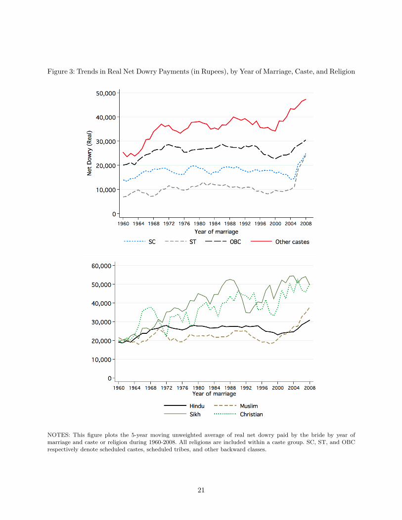
Figure 3: Trends in Real Net Dowry Payments (in Rupees), by Year of Marriage, Caste, and Religion

NOTES: This figure plots the 5-year moving unweighted average of real net dowry paid by the bride by year ofmarriage and caste or religion during 1960-2008. All religions are included within a caste group. SC, ST, and OBCrespectively denote scheduled castes, scheduled tribes, and other backward classes.

21

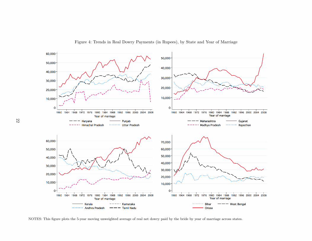
Figure 4: Trends in Real Dowry Payments (in Rupees), by State and Year of Marriage

NOTES: This figure plots the 5-year moving unweighted average of real net dowry paid by the bride by year of marriage across states.

22

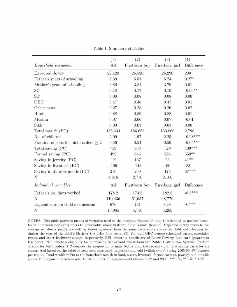
Table 1: Summary statistics

(1) (2) (3) (4)Household variables: All Firstborn boy Firstborn girl Difference

Expected dowry 26,420 26,520 26,290 230Father’s years of schooling 6.39 6.51 6.24 0.27*Mother’s years of schooling 3.80 3.81 3.79 0.01SC 0.18 0.17 0.19 -0.03**ST 0.08 0.08 0.08 0.00OBC 0.47 0.48 0.47 0.01Other caste 0.27 0.28 0.26 0.02Hindu 0.88 0.89 0.88 0.01Muslim 0.07 0.06 0.07 -0.01Sikh 0.03 0.03 0.03 0.00Total wealth (PC) 155,434 156,658 153,860 2,798No. of children 2.09 1.97 2.25 -0.28***Fraction of sons for birth orders ≥ 2 0.56 0.54 0.59 -0.05***Total saving (PC) 759 938 529 409***Formal saving (PC) 492 645 295 350**Saving in jewelry (PC) 119 137 96 41**Saving in livestock (PC) -106 -143 -60 -83Saving in durable goods (PC) 210 239 173 67***N 4,816 2,710 2,106

Individual variables: All Firstborn boy Firstborn girl Difference

Father’s no. days worked 178.2 174.5 182.8 -8.3***N 110,436 61,657 48,779Expenditure on child’s education 676 721 628 94***N 10,985 5,716 5,269

NOTES: This table provides means of variables used in the analysis. Household data is restricted to nuclear house-holds. Firstborn boy (girl) refers to households whose firstborn child is male (female). Expected dowry refers to theaverage net dowry paid (received) by brides (grooms) from the same caste and state as the child and who marriedduring the year of the child’s birth or the prior four years. SC, ST, and OBC denote scheduled castes, scheduledtribes, and other backward classes, respectively. BPL denote a beneficiary of Below Poverty Line card (poorest orless poor). PDS denote a eligibility for purchasing rice or/and wheat from the Public Distribution System. Fractionof sons for birth orders ≥ 2 denotes the proportion of male births from the second child. The saving variables areconstructed based on the value of each item purchased (deposits) and sold (withdrawals) during 2005-06. PC denotesper capita. Total wealth refers to the household wealth in land, assets, livestock, formal savings, jewelry, and durablegoods. Employment variables refer to the number of days worked between 1982 and 2006. *** 1%, ** 5%, * 10%.

23

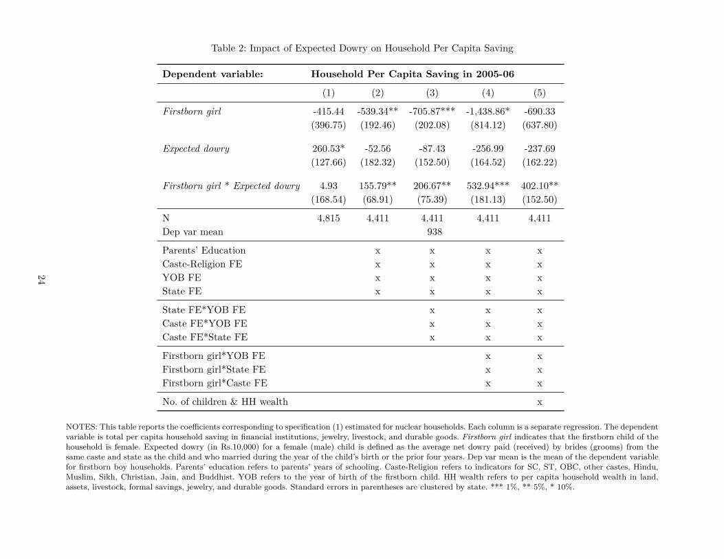
Table 2: Impact of Expected Dowry on Household Per Capita Saving

Dependent variable: Household Per Capita Saving in 2005-06

(1) (2) (3) (4) (5)

Firstborn girl -415.44 -539.34** -705.87*** -1,438.86* -690.33(396.75) (192.46) (202.08) (814.12) (637.80)

Expected dowry 260.53* -52.56 -87.43 -256.99 -237.69(127.66) (182.32) (152.50) (164.52) (162.22)

Firstborn girl * Expected dowry 4.93 155.79** 206.67** 532.94*** 402.10**(168.54) (68.91) (75.39) (181.13) (152.50)

N 4,815 4,411 4,411 4,411 4,411Dep var mean 938

Parents’ Education x x x xCaste-Religion FE x x x xYOB FE x x x xState FE x x x x

State FE*YOB FE x x xCaste FE*YOB FE x x xCaste FE*State FE x x x

Firstborn girl*YOB FE x xFirstborn girl*State FE x xFirstborn girl*Caste FE x x

No. of children & HH wealth x

NOTES: This table reports the coefficients corresponding to specification (1) estimated for nuclear households. Each column is a separate regression. The dependentvariable is total per capita household saving in financial institutions, jewelry, livestock, and durable goods. Firstborn girl indicates that the firstborn child of thehousehold is female. Expected dowry (in Rs.10,000) for a female (male) child is defined as the average net dowry paid (received) by brides (grooms) from thesame caste and state as the child and who married during the year of the child’s birth or the prior four years. Dep var mean is the mean of the dependent variablefor firstborn boy households. Parents’ education refers to parents’ years of schooling. Caste-Religion refers to indicators for SC, ST, OBC, other castes, Hindu,Muslim, Sikh, Christian, Jain, and Buddhist. YOB refers to the year of birth of the firstborn child. HH wealth refers to per capita household wealth in land,assets, livestock, formal savings, jewelry, and durable goods. Standard errors in parentheses are clustered by state. *** 1%, ** 5%, * 10%.

24

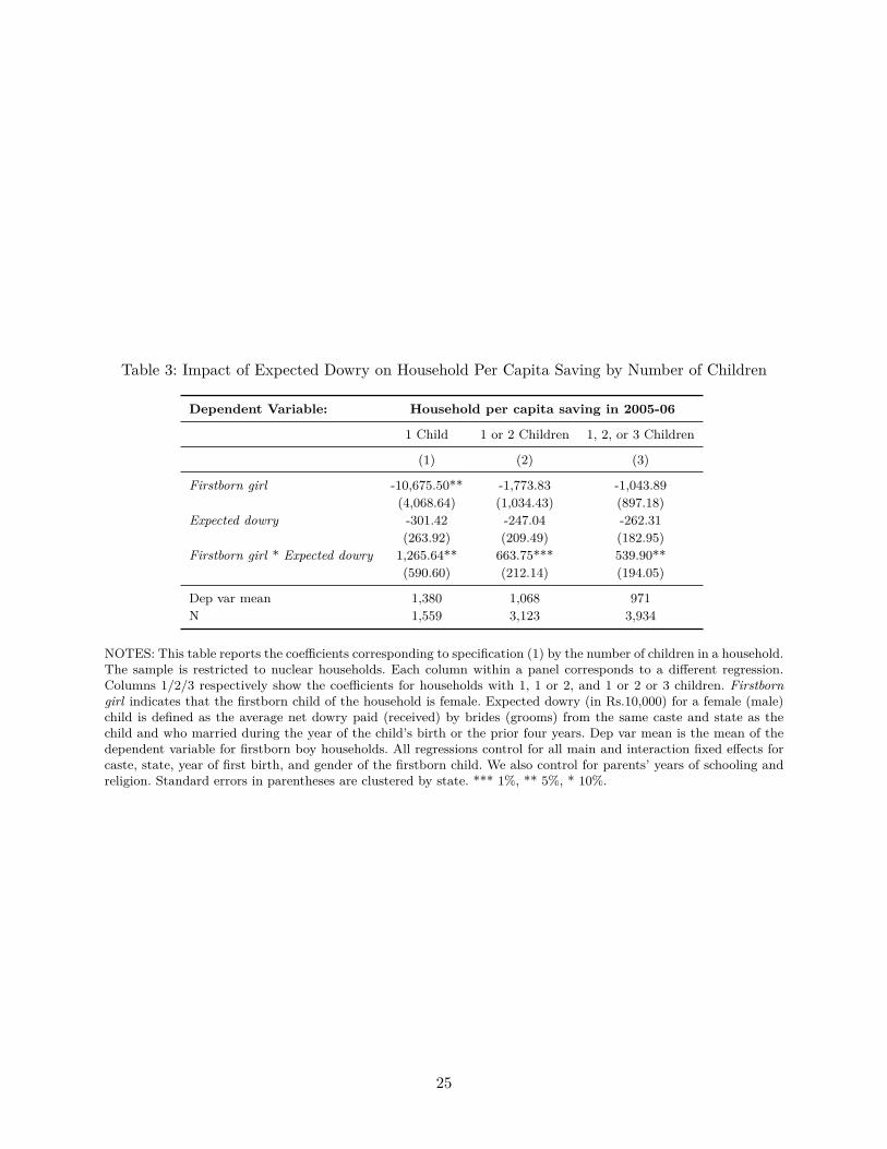
Table 3: Impact of Expected Dowry on Household Per Capita Saving by Number of Children

Dependent Variable: Household per capita saving in 2005-06

1 Child 1 or 2 Children 1, 2, or 3 Children

(1) (2) (3)

Firstborn girl -10,675.50** -1,773.83 -1,043.89(4,068.64) (1,034.43) (897.18)

Expected dowry -301.42 -247.04 -262.31(263.92) (209.49) (182.95)

Firstborn girl * Expected dowry 1,265.64** 663.75*** 539.90**(590.60) (212.14) (194.05)

Dep var mean 1,380 1,068 971N 1,559 3,123 3,934

NOTES: This table reports the coefficients corresponding to specification (1) by the number of children in a household.The sample is restricted to nuclear households. Each column within a panel corresponds to a different regression.Columns 1/2/3 respectively show the coefficients for households with 1, 1 or 2, and 1 or 2 or 3 children. Firstborngirl indicates that the firstborn child of the household is female. Expected dowry (in Rs.10,000) for a female (male)child is defined as the average net dowry paid (received) by brides (grooms) from the same caste and state as thechild and who married during the year of the child’s birth or the prior four years. Dep var mean is the mean of thedependent variable for firstborn boy households. All regressions control for all main and interaction fixed effects forcaste, state, year of first birth, and gender of the firstborn child. We also control for parents’ years of schooling andreligion. Standard errors in parentheses are clustered by state. *** 1%, ** 5%, * 10%.

25

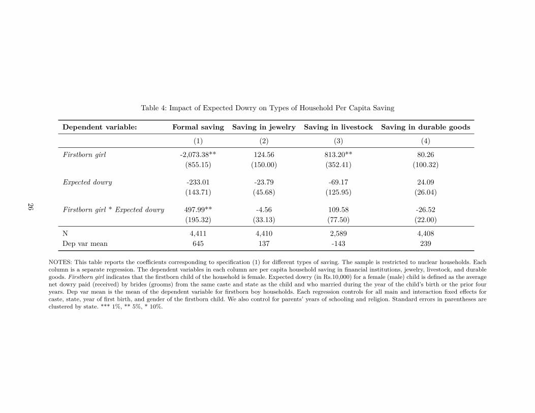
Table 4: Impact of Expected Dowry on Types of Household Per Capita Saving

Dependent variable: Formal saving Saving in jewelry Saving in livestock Saving in durable goods

(1) (2) (3) (4)

Firstborn girl -2,073.38** 124.56 813.20** 80.26(855.15) (150.00) (352.41) (100.32)

Expected dowry -233.01 -23.79 -69.17 24.09(143.71) (45.68) (125.95) (26.04)

Firstborn girl * Expected dowry 497.99** -4.56 109.58 -26.52(195.32) (33.13) (77.50) (22.00)

N 4,411 4,410 2,589 4,408Dep var mean 645 137 -143 239

NOTES: This table reports the coefficients corresponding to specification (1) for different types of saving. The sample is restricted to nuclear households. Eachcolumn is a separate regression. The dependent variables in each column are per capita household saving in financial institutions, jewelry, livestock, and durablegoods. Firstborn girl indicates that the firstborn child of the household is female. Expected dowry (in Rs.10,000) for a female (male) child is defined as the averagenet dowry paid (received) by brides (grooms) from the same caste and state as the child and who married during the year of the child’s birth or the prior fouryears. Dep var mean is the mean of the dependent variable for firstborn boy households. Each regression controls for all main and interaction fixed effects forcaste, state, year of first birth, and gender of the firstborn child. We also control for parents’ years of schooling and religion. Standard errors in parentheses areclustered by state. *** 1%, ** 5%, * 10%.

26

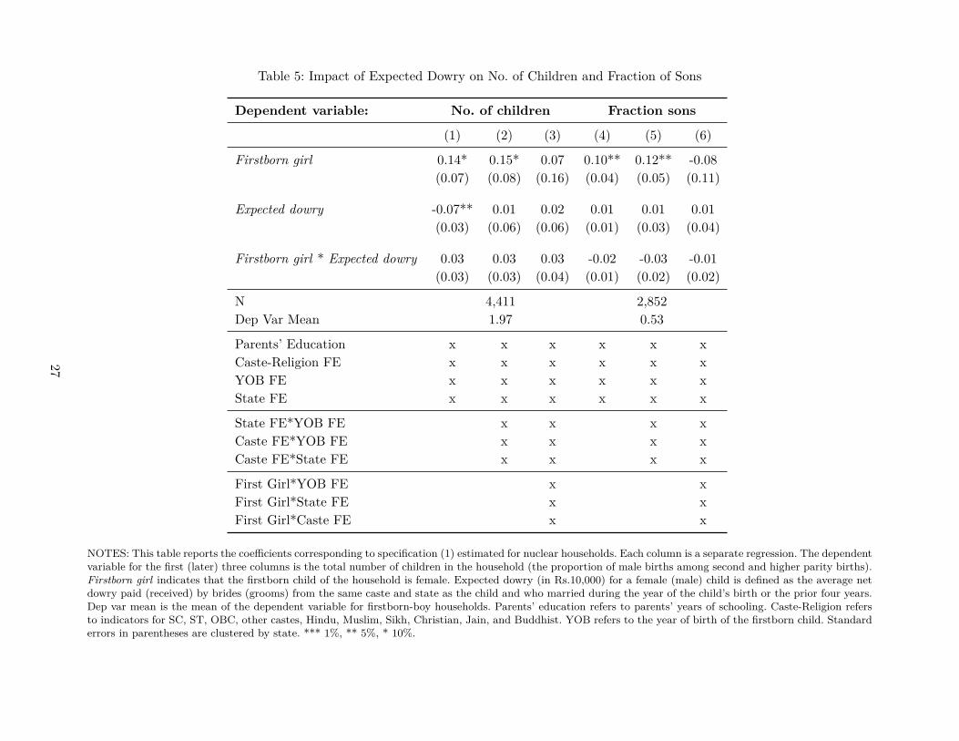
Table 5: Impact of Expected Dowry on No. of Children and Fraction of Sons

Dependent variable: No. of children Fraction sons

(1) (2) (3) (4) (5) (6)

Firstborn girl 0.14* 0.15* 0.07 0.10** 0.12** -0.08(0.07) (0.08) (0.16) (0.04) (0.05) (0.11)

Expected dowry -0.07** 0.01 0.02 0.01 0.01 0.01(0.03) (0.06) (0.06) (0.01) (0.03) (0.04)

Firstborn girl * Expected dowry 0.03 0.03 0.03 -0.02 -0.03 -0.01(0.03) (0.03) (0.04) (0.01) (0.02) (0.02)

N 4,411 2,852Dep Var Mean 1.97 0.53

Parents’ Education x x x x x xCaste-Religion FE x x x x x xYOB FE x x x x x xState FE x x x x x x

State FE*YOB FE x x x xCaste FE*YOB FE x x x xCaste FE*State FE x x x x

First Girl*YOB FE x xFirst Girl*State FE x xFirst Girl*Caste FE x x

NOTES: This table reports the coefficients corresponding to specification (1) estimated for nuclear households. Each column is a separate regression. The dependentvariable for the first (later) three columns is the total number of children in the household (the proportion of male births among second and higher parity births).Firstborn girl indicates that the firstborn child of the household is female. Expected dowry (in Rs.10,000) for a female (male) child is defined as the average netdowry paid (received) by brides (grooms) from the same caste and state as the child and who married during the year of the child’s birth or the prior four years.Dep var mean is the mean of the dependent variable for firstborn-boy households. Parents’ education refers to parents’ years of schooling. Caste-Religion refersto indicators for SC, ST, OBC, other castes, Hindu, Muslim, Sikh, Christian, Jain, and Buddhist. YOB refers to the year of birth of the firstborn child. Standarderrors in parentheses are clustered by state. *** 1%, ** 5%, * 10%.

27

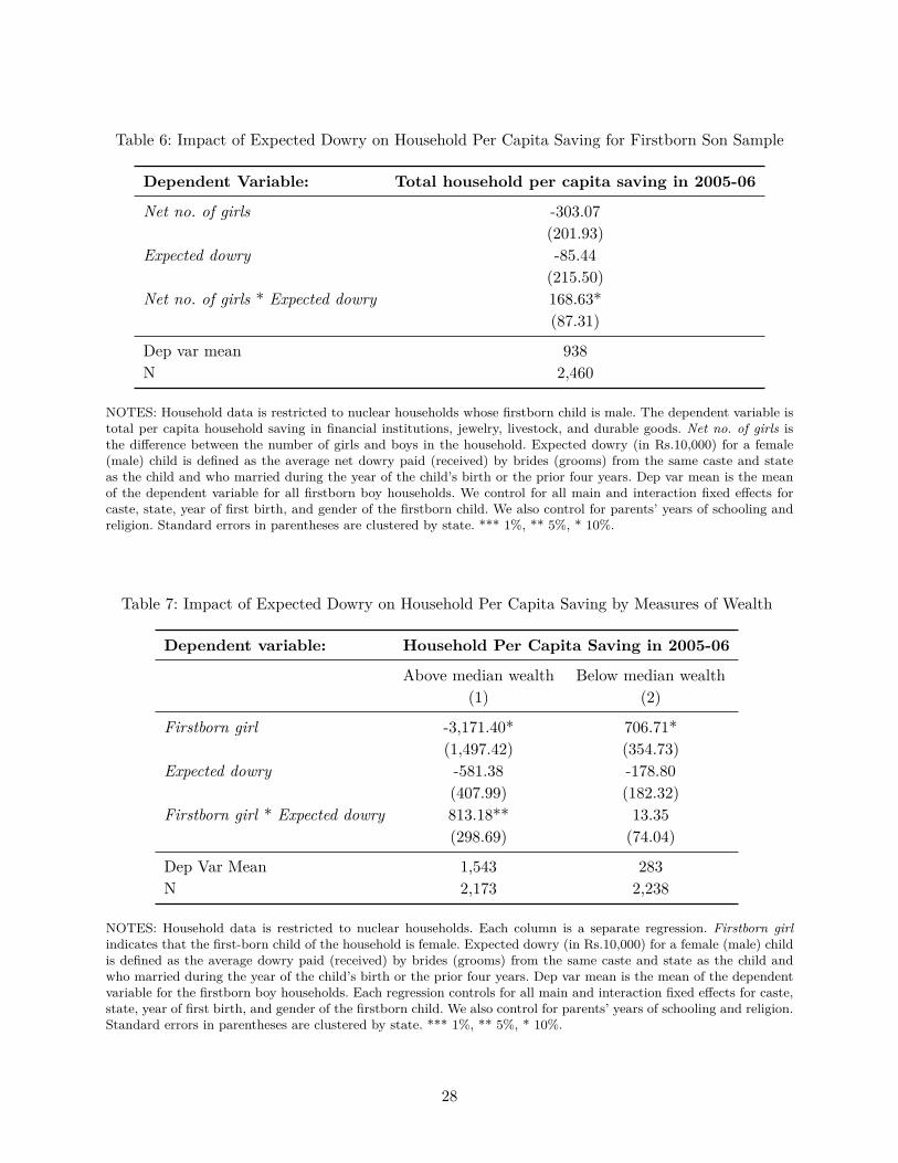
Table 6: Impact of Expected Dowry on Household Per Capita Saving for Firstborn Son Sample

Dependent Variable: Total household per capita saving in 2005-06

Net no. of girls -303.07(201.93)

Expected dowry -85.44(215.50)

Net no. of girls * Expected dowry 168.63*(87.31)

Dep var mean 938N 2,460

NOTES: Household data is restricted to nuclear households whose firstborn child is male. The dependent variable istotal per capita household saving in financial institutions, jewelry, livestock, and durable goods. Net no. of girls isthe difference between the number of girls and boys in the household. Expected dowry (in Rs.10,000) for a female(male) child is defined as the average net dowry paid (received) by brides (grooms) from the same caste and stateas the child and who married during the year of the child’s birth or the prior four years. Dep var mean is the meanof the dependent variable for all firstborn boy households. We control for all main and interaction fixed effects forcaste, state, year of first birth, and gender of the firstborn child. We also control for parents’ years of schooling andreligion. Standard errors in parentheses are clustered by state. *** 1%, ** 5%, * 10%.

Table 7: Impact of Expected Dowry on Household Per Capita Saving by Measures of Wealth

Dependent variable: Household Per Capita Saving in 2005-06

Above median wealth Below median wealth(1) (2)

Firstborn girl -3,171.40* 706.71*(1,497.42) (354.73)

Expected dowry -581.38 -178.80(407.99) (182.32)

Firstborn girl * Expected dowry 813.18** 13.35(298.69) (74.04)

Dep Var Mean 1,543 283N 2,173 2,238

NOTES: Household data is restricted to nuclear households. Each column is a separate regression. Firstborn girlindicates that the first-born child of the household is female. Expected dowry (in Rs.10,000) for a female (male) childis defined as the average dowry paid (received) by brides (grooms) from the same caste and state as the child andwho married during the year of the child’s birth or the prior four years. Dep var mean is the mean of the dependentvariable for the firstborn boy households. Each regression controls for all main and interaction fixed effects for caste,state, year of first birth, and gender of the firstborn child. We also control for parents’ years of schooling and religion.Standard errors in parentheses are clustered by state. *** 1%, ** 5%, * 10%.

28

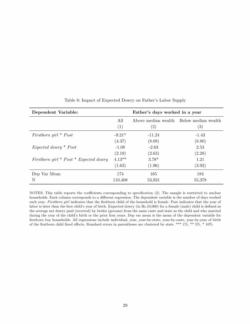
Table 8: Impact of Expected Dowry on Father’s Labor Supply

Dependent Variable: Father’s days worked in a year

All Above median wealth Below median wealth(1) (2) (3)

Firstborn girl * Post -9.21* -11.24 -1.43(4.37) (8.08) (8.80)

Expected dowry * Post -1.08 -2.63 2.53(2.19) (2.63) (2.28)

Firstborn girl * Post * Expected dowry 4.13** 3.78* 1.21(1.63) (1.96) (3.92)

Dep Var Mean 174 165 184N 110,408 53,931 55,378

NOTES: This table reports the coefficients corresponding to specification (2). The sample is restricted to nuclearhouseholds. Each column corresponds to a different regression. The dependent variable is the number of days workedeach year. Firstborn girl indicates that the firstborn child of the household is female. Post indicates that the year oflabor is later than the first child’s year of birth. Expected dowry (in Rs.10,000) for a female (male) child is defined asthe average net dowry paid (received) by brides (grooms) from the same caste and state as the child and who marriedduring the year of the child’s birth or the prior four years. Dep var mean is the mean of the dependent variable forfirstborn boy households. All regressions include individual, year, year-by-state, year-by-caste, year-by-year of birthof the firstborn child fixed effects. Standard errors in parentheses are clustered by state. *** 1%, ** 5%, * 10%.

29

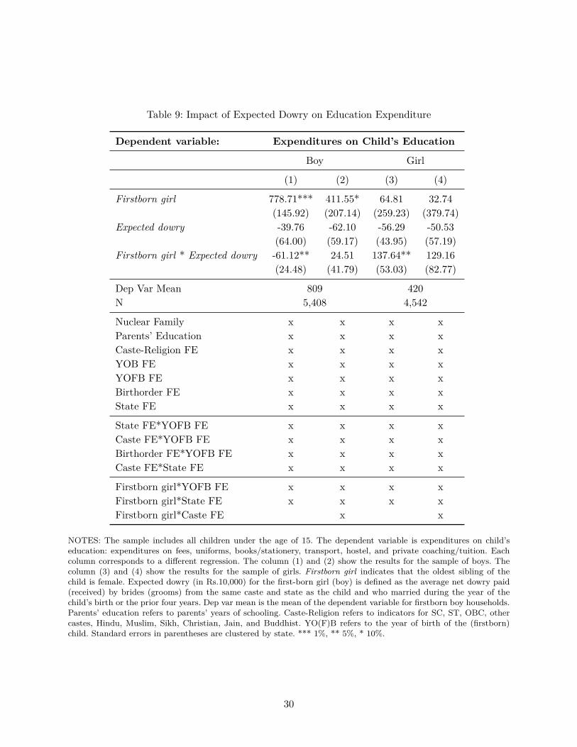
Table 9: Impact of Expected Dowry on Education Expenditure

Dependent variable: Expenditures on Child’s Education

Boy Girl

(1) (2) (3) (4)

Firstborn girl 778.71*** 411.55* 64.81 32.74(145.92) (207.14) (259.23) (379.74)

Expected dowry -39.76 -62.10 -56.29 -50.53(64.00) (59.17) (43.95) (57.19)

Firstborn girl * Expected dowry -61.12** 24.51 137.64** 129.16(24.48) (41.79) (53.03) (82.77)

Dep Var Mean 809 420N 5,408 4,542

Nuclear Family x x x xParents’ Education x x x xCaste-Religion FE x x x xYOB FE x x x xYOFB FE x x x xBirthorder FE x x x xState FE x x x x

State FE*YOFB FE x x x xCaste FE*YOFB FE x x x xBirthorder FE*YOFB FE x x x xCaste FE*State FE x x x x

Firstborn girl*YOFB FE x x x xFirstborn girl*State FE x x x xFirstborn girl*Caste FE x x

NOTES: The sample includes all children under the age of 15. The dependent variable is expenditures on child’seducation: expenditures on fees, uniforms, books/stationery, transport, hostel, and private coaching/tuition. Eachcolumn corresponds to a different regression. The column (1) and (2) show the results for the sample of boys. Thecolumn (3) and (4) show the results for the sample of girls. Firstborn girl indicates that the oldest sibling of thechild is female. Expected dowry (in Rs.10,000) for the first-born girl (boy) is defined as the average net dowry paid(received) by brides (grooms) from the same caste and state as the child and who married during the year of thechild’s birth or the prior four years. Dep var mean is the mean of the dependent variable for firstborn boy households.Parents’ education refers to parents’ years of schooling. Caste-Religion refers to indicators for SC, ST, OBC, othercastes, Hindu, Muslim, Sikh, Christian, Jain, and Buddhist. YO(F)B refers to the year of birth of the (firstborn)child. Standard errors in parentheses are clustered by state. *** 1%, ** 5%, * 10%.

30

A Appendix

Table A.1: Descriptive Statistics on Wedding Expenditure from the 2004-05 India Human Development Survey

Panel A: By caste

Urban RuralBrahmin OBC SC ST Others Brahmin OBC SC ST Others

(1) (2) (3) (4) (5) (6) (7) (8) (9) (10)

Expenditure by bride’s family 186,683 120,818 96,038 74,689 165,710 140,575 89,973 64,194 35,007 120,038Expenditure by groom’s family 128,166 74,673 63,616 58,691 108,188 92,365 56,380 43,539 29,176 74,162

Difference 58,617 46,145 32,423 15,997 57,522 48,210 33,589 20,655 5,835 45,875N 1,313 5,452 2,322 499 4,956 1,108 10,834 6,011 2,939 6,118

Panel B: By religion

Urban RuralHindu Muslim Christian Sikh Hindu Muslim Christian Sikh(1) (2) (3) (4) (5) (6) (7) (8)

Expenditure by bride’s family 137,992 119,959 143,553 194,341 84,014 100,849 103,211 161,513Expenditure by groom’s family 90,649 76,515 66,274 132,988 55,309 57,894 48,767 107,471

Difference 47,350 43,444 77,278 61,353 28,706 42,956 54,443 54,042N 11,286 2,215 514 258 22,239 2,573 862 732

NOTES: This table provides means of wedding expenditure in the 2004-05 India Human Development Survey (IHDS). The survey asks “At the time of themarriage in your community (jati) for a family like yours, how much money is usually spent by the girl(boy)’s family?” The IHDS data set has five broad socialgroups: (1) Brahmin (2) OBC (3) SC (4) ST (5) Others.

31

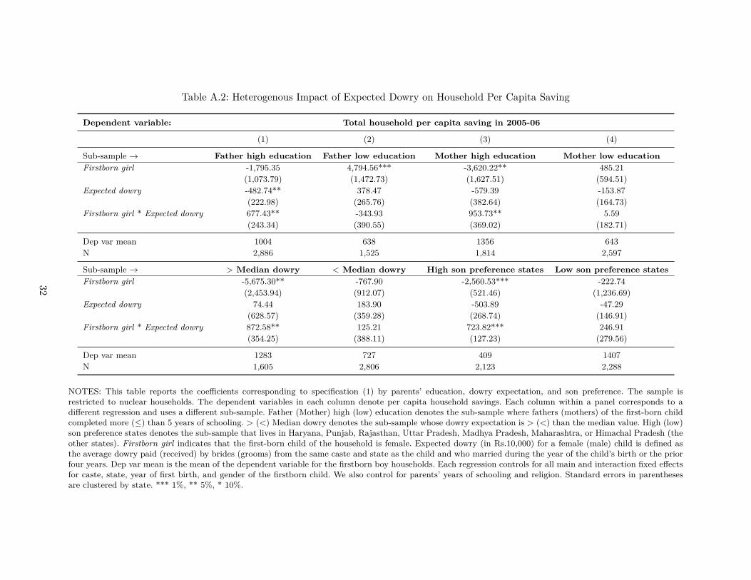
Table A.2: Heterogenous Impact of Expected Dowry on Household Per Capita Saving

Dependent variable: Total household per capita saving in 2005-06

(1) (2) (3) (4)

Sub-sample → Father high education Father low education Mother high education Mother low educationFirstborn girl -1,795.35 4,794.56*** -3,620.22** 485.21

(1,073.79) (1,472.73) (1,627.51) (594.51)Expected dowry -482.74** 378.47 -579.39 -153.87

(222.98) (265.76) (382.64) (164.73)Firstborn girl * Expected dowry 677.43** -343.93 953.73** 5.59

(243.34) (390.55) (369.02) (182.71)

Dep var mean 1004 638 1356 643N 2,886 1,525 1,814 2,597

Sub-sample → > Median dowry < Median dowry High son preference states Low son preference statesFirstborn girl -5,675.30** -767.90 -2,560.53*** -222.74

(2,453.94) (912.07) (521.46) (1,236.69)Expected dowry 74.44 183.90 -503.89 -47.29

(628.57) (359.28) (268.74) (146.91)Firstborn girl * Expected dowry 872.58** 125.21 723.82*** 246.91

(354.25) (388.11) (127.23) (279.56)

Dep var mean 1283 727 409 1407N 1,605 2,806 2,123 2,288

NOTES: This table reports the coefficients corresponding to specification (1) by parents’ education, dowry expectation, and son preference. The sample isrestricted to nuclear households. The dependent variables in each column denote per capita household savings. Each column within a panel corresponds to adifferent regression and uses a different sub-sample. Father (Mother) high (low) education denotes the sub-sample where fathers (mothers) of the first-born childcompleted more (≤) than 5 years of schooling. > (<) Median dowry denotes the sub-sample whose dowry expectation is > (<) than the median value. High (low)son preference states denotes the sub-sample that lives in Haryana, Punjab, Rajasthan, Uttar Pradesh, Madhya Pradesh, Maharashtra, or Himachal Pradesh (theother states). Firstborn girl indicates that the first-born child of the household is female. Expected dowry (in Rs.10,000) for a female (male) child is defined asthe average dowry paid (received) by brides (grooms) from the same caste and state as the child and who married during the year of the child’s birth or the priorfour years. Dep var mean is the mean of the dependent variable for the firstborn boy households. Each regression controls for all main and interaction fixed effectsfor caste, state, year of first birth, and gender of the firstborn child. We also control for parents’ years of schooling and religion. Standard errors in parenthesesare clustered by state. *** 1%, ** 5%, * 10%.

32

Table A.3: Impact of Expected Dowry Defined using Caste and Religion on Household Per Capita Saving

Dependent variable: Total household per capita saving in 2005-06

(1) (2) (3) (4) (5)

Firstborn girl -484.81 -477.51*** -602.56*** -373.95 -219.17(329.23) (160.16) (171.85) (587.25) (564.77)

Expected dowry 170.85 -105.16 33.41 -21.63 24.28(133.84) (146.99) (167.44) (166.13) (188.97)

Firstborn girl * Expected dowry 30.36 130.33** 167.61** 264.49* 272.68**(138.58) (55.45) (60.10) (126.61) (120.66)

N 4,811 4,407 4,407 4,407 4,407Dep var mean 938

Parents’ Education x x x xCaste-Religion FE x x x xYOB FE x x x xState FE x x x x

State FE*YOB FE x x xCaste FE*YOB FE x x xCaste FE*State FE x x x

Firstborn girl*YOB FE x xFirstborn girl*State FE x xFirstborn girl*Caste FE x x

No. of children & HH wealth x

NOTES: This table reports the coefficients corresponding to specification (1) estimated for nuclear households. Each column is a separate regression. The dependentvariable is total per capita household saving in financial institutions, jewelry, livestock, and durable goods. Firstborn girl indicates that the firstborn child ofthe household is female. Expected dowry (in Rs.10,000) for a female (male) child is defined as the average dowry paid (received) by brides (grooms) from thesame social group and state as the child and who married during the year of the child’s birth or the prior four years. We construct seven social groups basedon the caste and religion. Specifically, we split Hindus by caste and use other religions as it is (i.e., Hindu SCs, Hindu STs, Hindu OBCs, Hindu OCs, Muslims,Sikhs, Other religions). Dep var mean is the mean of the dependent variable for firstborn boy households. Parents’ education refers to parents’ years of schooling.Caste-Religion refers to indicators for SC, ST, OBC, other castes, Hindu, Muslim, Sikh, Christian, Jain, and Buddhist. HH wealth refers to per capita householdwealth in land, assets, livestock, formal savings, jewelry, and durable goods. Standard errors in parentheses are clustered by state. *** 1%, ** 5%, * 10%.

33

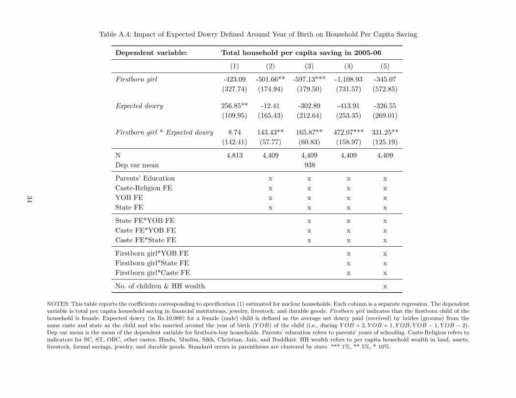
Table A.4: Impact of Expected Dowry Defined Around Year of Birth on Household Per Capita Saving

Dependent variable: Total household per capita saving in 2005-06

(1) (2) (3) (4) (5)

Firstborn girl -423.09 -501.66** -597.13*** -1,108.93 -345.07(327.74) (174.94) (179.50) (731.57) (572.85)

Expected dowry 256.85** -12.41 -302.89 -413.91 -326.55(109.95) (165.43) (212.64) (253.35) (269.01)

Firstborn girl * Expected dowry 8.74 143.43** 165.87** 472.07*** 331.25**(142.41) (57.77) (60.83) (158.97) (125.19)

N 4,813 4,409 4,409 4,409 4,409Dep var mean 938

Parents’ Education x x x xCaste-Religion FE x x x xYOB FE x x x xState FE x x x x

State FE*YOB FE x x xCaste FE*YOB FE x x xCaste FE*State FE x x x

Firstborn girl*YOB FE x xFirstborn girl*State FE x xFirstborn girl*Caste FE x x

No. of children & HH wealth x

NOTES: This table reports the coefficients corresponding to specification (1) estimated for nuclear households. Each column is a separate regression. The dependentvariable is total per capita household saving in financial institutions, jewelry, livestock, and durable goods. Firstborn girl indicates that the firstborn child of thehousehold is female. Expected dowry (in Rs.10,000) for a female (male) child is defined as the average net dowry paid (received) by brides (grooms) from thesame caste and state as the child and who married around the year of birth (Y OB) of the child (i.e., during Y OB + 2, Y OB + 1, Y OB, Y OB − 1, Y OB − 2).Dep var mean is the mean of the dependent variable for firstborn-boy households. Parents’ education refers to parents’ years of schooling. Caste-Religion refers toindicators for SC, ST, OBC, other castes, Hindu, Muslim, Sikh, Christian, Jain, and Buddhist. HH wealth refers to per capita household wealth in land, assets,livestock, formal savings, jewelry, and durable goods. Standard errors in parentheses are clustered by state. *** 1%, ** 5%, * 10%.

34

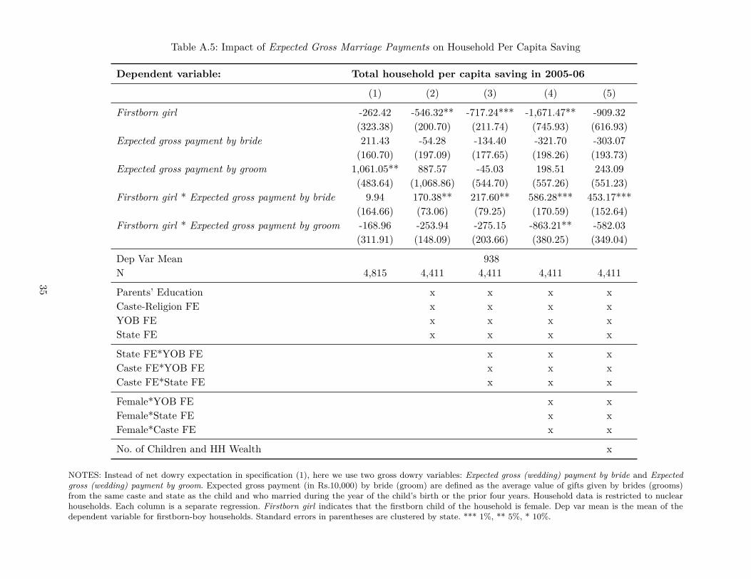
Table A.5: Impact of Expected Gross Marriage Payments on Household Per Capita Saving

Dependent variable: Total household per capita saving in 2005-06

(1) (2) (3) (4) (5)

Firstborn girl -262.42 -546.32** -717.24*** -1,671.47** -909.32(323.38) (200.70) (211.74) (745.93) (616.93)

Expected gross payment by bride 211.43 -54.28 -134.40 -321.70 -303.07(160.70) (197.09) (177.65) (198.26) (193.73)

Expected gross payment by groom 1,061.05** 887.57 -45.03 198.51 243.09(483.64) (1,068.86) (544.70) (557.26) (551.23)

Firstborn girl * Expected gross payment by bride 9.94 170.38** 217.60** 586.28*** 453.17***(164.66) (73.06) (79.25) (170.59) (152.64)

Firstborn girl * Expected gross payment by groom -168.96 -253.94 -275.15 -863.21** -582.03(311.91) (148.09) (203.66) (380.25) (349.04)

Dep Var Mean 938N 4,815 4,411 4,411 4,411 4,411

Parents’ Education x x x xCaste-Religion FE x x x xYOB FE x x x xState FE x x x x

State FE*YOB FE x x xCaste FE*YOB FE x x xCaste FE*State FE x x x

Female*YOB FE x xFemale*State FE x xFemale*Caste FE x x

No. of Children and HH Wealth x

NOTES: Instead of net dowry expectation in specification (1), here we use two gross dowry variables: Expected gross (wedding) payment by bride and Expectedgross (wedding) payment by groom. Expected gross payment (in Rs.10,000) by bride (groom) are defined as the average value of gifts given by brides (grooms)from the same caste and state as the child and who married during the year of the child’s birth or the prior four years. Household data is restricted to nuclearhouseholds. Each column is a separate regression. Firstborn girl indicates that the firstborn child of the household is female. Dep var mean is the mean of thedependent variable for firstborn-boy households. Standard errors in parentheses are clustered by state. *** 1%, ** 5%, * 10%.

35

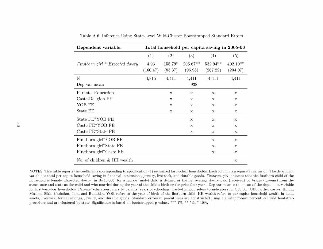
Table A.6: Inference Using State-Level Wild-Cluster Bootstrapped Standard Errors

Dependent variable: Total household per capita saving in 2005-06

(1) (2) (3) (4) (5)

Firstborn girl * Expected dowry 4.93 155.79* 206.67** 532.94** 402.10**(160.47) (83.37) (96.98) (267.22) (204.07)

N 4,815 4,411 4,411 4,411 4,411Dep var mean 938

Parents’ Education x x x xCaste-Religion FE x x x xYOB FE x x x xState FE x x x x

State FE*YOB FE x x xCaste FE*YOB FE x x xCaste FE*State FE x x x

Firstborn girl*YOB FE x xFirstborn girl*State FE x xFirstborn girl*Caste FE x x

No. of children & HH wealth x

NOTES: This table reports the coefficients corresponding to specification (1) estimated for nuclear households. Each column is a separate regression. The dependentvariable is total per capita household saving in financial institutions, jewelry, livestock, and durable goods. Firstborn girl indicates that the firstborn child of thehousehold is female. Expected dowry (in Rs.10,000) for a female (male) child is defined as the net average dowry paid (received) by brides (grooms) from thesame caste and state as the child and who married during the year of the child’s birth or the prior four years. Dep var mean is the mean of the dependent variablefor firstborn-boy households. Parents’ education refers to parents’ years of schooling. Caste-Religion refers to indicators for SC, ST, OBC, other castes, Hindu,Muslim, Sikh, Christian, Jain, and Buddhist. YOB refers to the year of birth of the firstborn child. HH wealth refers to per capita household wealth in land,assets, livestock, formal savings, jewelry, and durable goods. Standard errors in parentheses are constructed using a cluster robust percentile-t wild bootstrapprocedure and are clustered by state. Significance is based on bootstrapped p-values. *** 1%, ** 5%, * 10%.

36

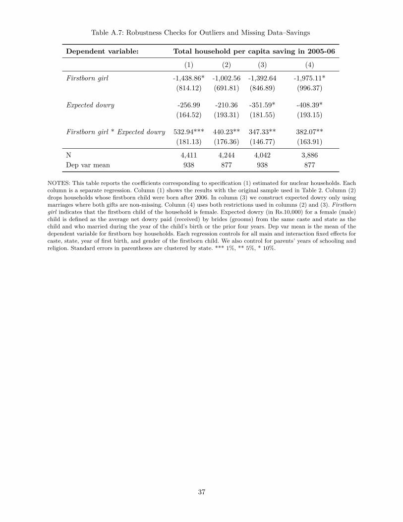
Table A.7: Robustness Checks for Outliers and Missing Data–Savings

Dependent variable: Total household per capita saving in 2005-06

(1) (2) (3) (4)

Firstborn girl -1,438.86* -1,002.56 -1,392.64 -1,975.11*(814.12) (691.81) (846.89) (996.37)

Expected dowry -256.99 -210.36 -351.59* -408.39*(164.52) (193.31) (181.55) (193.15)

Firstborn girl * Expected dowry 532.94*** 440.23** 347.33** 382.07**(181.13) (176.36) (146.77) (163.91)

N 4,411 4,244 4,042 3,886Dep var mean 938 877 938 877

NOTES: This table reports the coefficients corresponding to specification (1) estimated for nuclear households. Eachcolumn is a separate regression. Column (1) shows the results with the original sample used in Table 2. Column (2)drops households whose firstborn child were born after 2006. In column (3) we construct expected dowry only usingmarriages where both gifts are non-missing. Column (4) uses both restrictions used in columns (2) and (3). Firstborngirl indicates that the firstborn child of the household is female. Expected dowry (in Rs.10,000) for a female (male)child is defined as the average net dowry paid (received) by brides (grooms) from the same caste and state as thechild and who married during the year of the child’s birth or the prior four years. Dep var mean is the mean of thedependent variable for firstborn boy households. Each regression controls for all main and interaction fixed effects forcaste, state, year of first birth, and gender of the firstborn child. We also control for parents’ years of schooling andreligion. Standard errors in parentheses are clustered by state. *** 1%, ** 5%, * 10%.

37

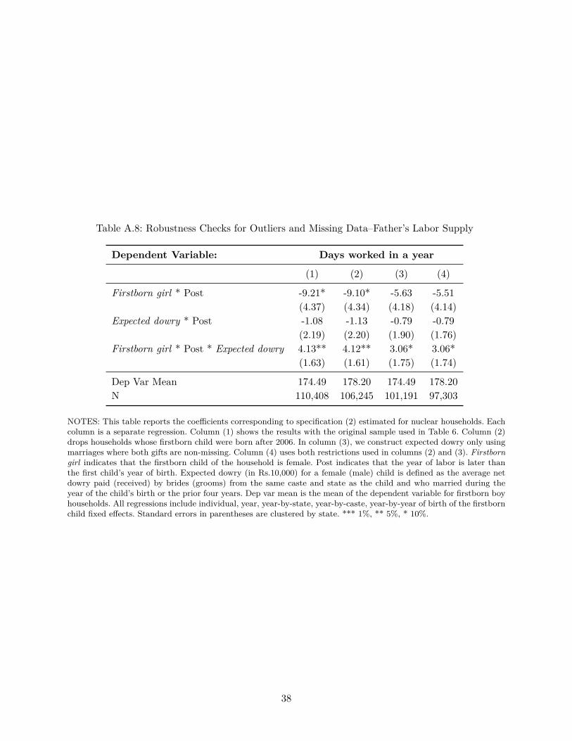
Table A.8: Robustness Checks for Outliers and Missing Data–Father’s Labor Supply

Dependent Variable: Days worked in a year

(1) (2) (3) (4)

Firstborn girl * Post -9.21* -9.10* -5.63 -5.51(4.37) (4.34) (4.18) (4.14)

Expected dowry * Post -1.08 -1.13 -0.79 -0.79(2.19) (2.20) (1.90) (1.76)

Firstborn girl * Post * Expected dowry 4.13** 4.12** 3.06* 3.06*(1.63) (1.61) (1.75) (1.74)

Dep Var Mean 174.49 178.20 174.49 178.20N 110,408 106,245 101,191 97,303

NOTES: This table reports the coefficients corresponding to specification (2) estimated for nuclear households. Eachcolumn is a separate regression. Column (1) shows the results with the original sample used in Table 6. Column (2)drops households whose firstborn child were born after 2006. In column (3), we construct expected dowry only usingmarriages where both gifts are non-missing. Column (4) uses both restrictions used in columns (2) and (3). Firstborngirl indicates that the firstborn child of the household is female. Post indicates that the year of labor is later thanthe first child’s year of birth. Expected dowry (in Rs.10,000) for a female (male) child is defined as the average netdowry paid (received) by brides (grooms) from the same caste and state as the child and who married during theyear of the child’s birth or the prior four years. Dep var mean is the mean of the dependent variable for firstborn boyhouseholds. All regressions include individual, year, year-by-state, year-by-caste, year-by-year of birth of the firstbornchild fixed effects. Standard errors in parentheses are clustered by state. *** 1%, ** 5%, * 10%.

38

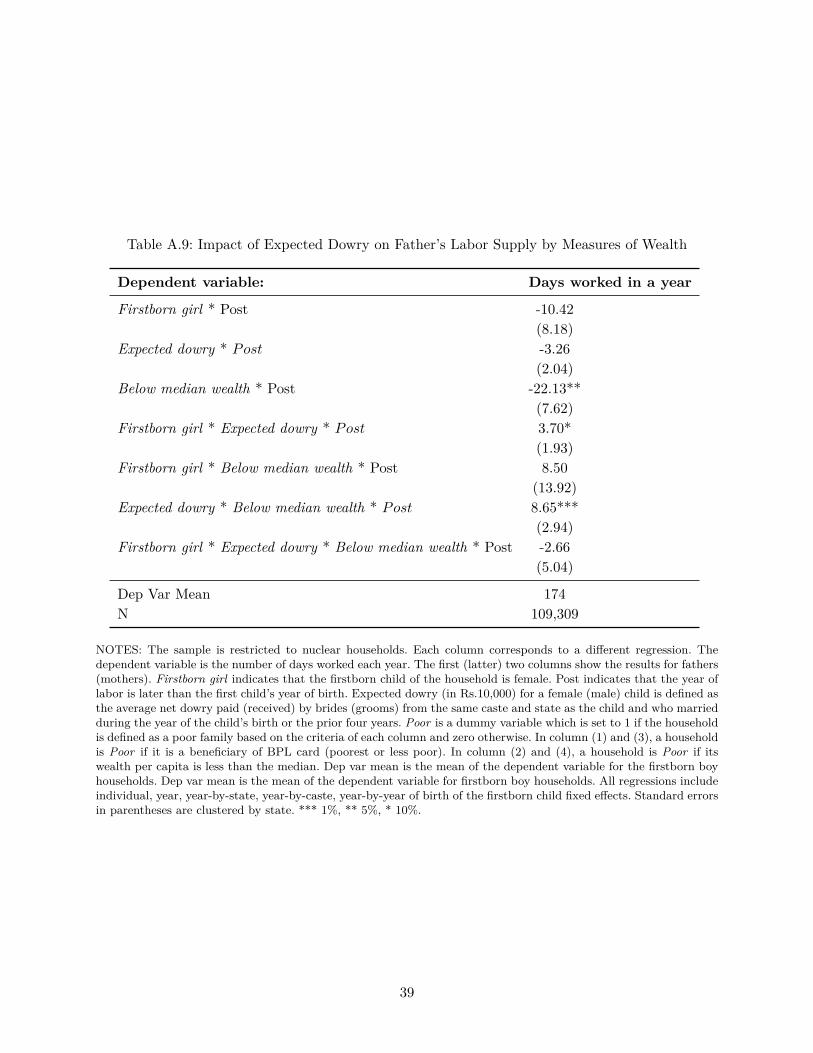
Table A.9: Impact of Expected Dowry on Father’s Labor Supply by Measures of Wealth

Dependent variable: Days worked in a year

Firstborn girl * Post -10.42(8.18)

Expected dowry * Post -3.26(2.04)

Below median wealth * Post -22.13**(7.62)

Firstborn girl * Expected dowry * Post 3.70*(1.93)

Firstborn girl * Below median wealth * Post 8.50(13.92)

Expected dowry * Below median wealth * Post 8.65***(2.94)

Firstborn girl * Expected dowry * Below median wealth * Post -2.66(5.04)

Dep Var Mean 174N 109,309

NOTES: The sample is restricted to nuclear households. Each column corresponds to a different regression. Thedependent variable is the number of days worked each year. The first (latter) two columns show the results for fathers(mothers). Firstborn girl indicates that the firstborn child of the household is female. Post indicates that the year oflabor is later than the first child’s year of birth. Expected dowry (in Rs.10,000) for a female (male) child is defined asthe average net dowry paid (received) by brides (grooms) from the same caste and state as the child and who marriedduring the year of the child’s birth or the prior four years. Poor is a dummy variable which is set to 1 if the householdis defined as a poor family based on the criteria of each column and zero otherwise. In column (1) and (3), a householdis Poor if it is a beneficiary of BPL card (poorest or less poor). In column (2) and (4), a household is Poor if itswealth per capita is less than the median. Dep var mean is the mean of the dependent variable for the firstborn boyhouseholds. Dep var mean is the mean of the dependent variable for firstborn boy households. All regressions includeindividual, year, year-by-state, year-by-caste, year-by-year of birth of the firstborn child fixed effects. Standard errorsin parentheses are clustered by state. *** 1%, ** 5%, * 10%.

39

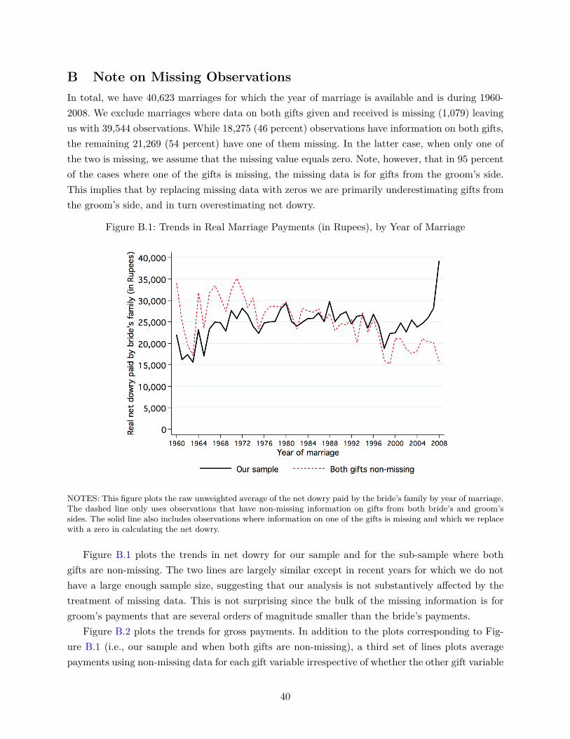
B Note on Missing ObservationsIn total, we have 40,623 marriages for which the year of marriage is available and is during 1960-2008. We exclude marriages where data on both gifts given and received is missing (1,079) leavingus with 39,544 observations. While 18,275 (46 percent) observations have information on both gifts,the remaining 21,269 (54 percent) have one of them missing. In the latter case, when only one ofthe two is missing, we assume that the missing value equals zero. Note, however, that in 95 percentof the cases where one of the gifts is missing, the missing data is for gifts from the groom’s side.This implies that by replacing missing data with zeros we are primarily underestimating gifts fromthe groom’s side, and in turn overestimating net dowry.

Figure B.1: Trends in Real Marriage Payments (in Rupees), by Year of Marriage

NOTES: This figure plots the raw unweighted average of the net dowry paid by the bride’s family by year of marriage.The dashed line only uses observations that have non-missing information on gifts from both bride’s and groom’ssides. The solid line also includes observations where information on one of the gifts is missing and which we replacewith a zero in calculating the net dowry.

Figure B.1 plots the trends in net dowry for our sample and for the sub-sample where bothgifts are non-missing. The two lines are largely similar except in recent years for which we do nothave a large enough sample size, suggesting that our analysis is not substantively affected by thetreatment of missing data. This is not surprising since the bulk of the missing information is forgroom’s payments that are several orders of magnitude smaller than the bride’s payments.

Figure B.2 plots the trends for gross payments. In addition to the plots corresponding to Fig-ure B.1 (i.e., our sample and when both gifts are non-missing), a third set of lines plots averagepayments using non-missing data for each gift variable irrespective of whether the other gift variable

40

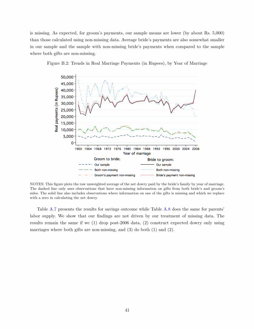
is missing. As expected, for groom’s payments, our sample means are lower (by about Rs. 5,000)than those calculated using non-missing data. Average bride’s payments are also somewhat smallerin our sample and the sample with non-missing bride’s payments when compared to the samplewhere both gifts are non-missing.

Figure B.2: Trends in Real Marriage Payments (in Rupees), by Year of Marriage

NOTES: This figure plots the raw unweighted average of the net dowry paid by the bride’s family by year of marriage.The dashed line only uses observations that have non-missing information on gifts from both bride’s and groom’ssides. The solid line also includes observations where information on one of the gifts is missing and which we replacewith a zero in calculating the net dowry.

Table A.7 presents the results for savings outcome while Table A.8 does the same for parents’labor supply. We show that our findings are not driven by our treatment of missing data. Theresults remain the same if we (1) drop post-2006 data, (2) construct expected dowry only usingmarriages where both gifts are non-missing, and (3) do both (1) and (2).

41

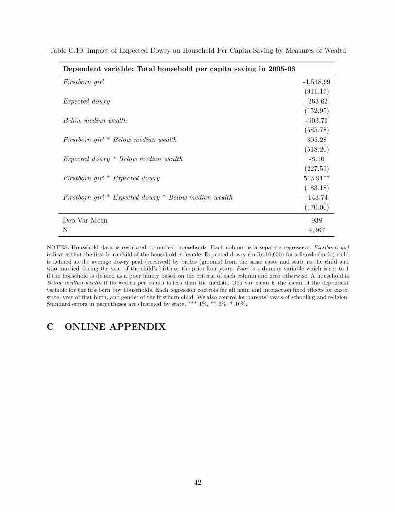
Table C.10: Impact of Expected Dowry on Household Per Capita Saving by Measures of Wealth

Dependent variable: Total household per capita saving in 2005-06

Firstborn girl -1,548.99(911.17)

Expected dowry -263.62(152.95)

Below median wealth -903.70(585.78)

Firstborn girl * Below median wealth 805.28(518.20)

Expected dowry * Below median wealth -8.10(227.51)

Firstborn girl * Expected dowry 513.91**(183.18)

Firstborn girl * Expected dowry * Below median wealth -143.74(170.00)

Dep Var Mean 938N 4,367

NOTES: Household data is restricted to nuclear households. Each column is a separate regression. Firstborn girlindicates that the first-born child of the household is female. Expected dowry (in Rs.10,000) for a female (male) childis defined as the average dowry paid (received) by brides (grooms) from the same caste and state as the child andwho married during the year of the child’s birth or the prior four years. Poor is a dummy variable which is set to 1if the household is defined as a poor family based on the criteria of each column and zero otherwise. A household isBelow median wealth if its wealth per capita is less than the median. Dep var mean is the mean of the dependentvariable for the firstborn boy households. Each regression controls for all main and interaction fixed effects for caste,state, year of first birth, and gender of the firstborn child. We also control for parents’ years of schooling and religion.Standard errors in parentheses are clustered by state. *** 1%, ** 5%, * 10%.

C ONLINE APPENDIX

42

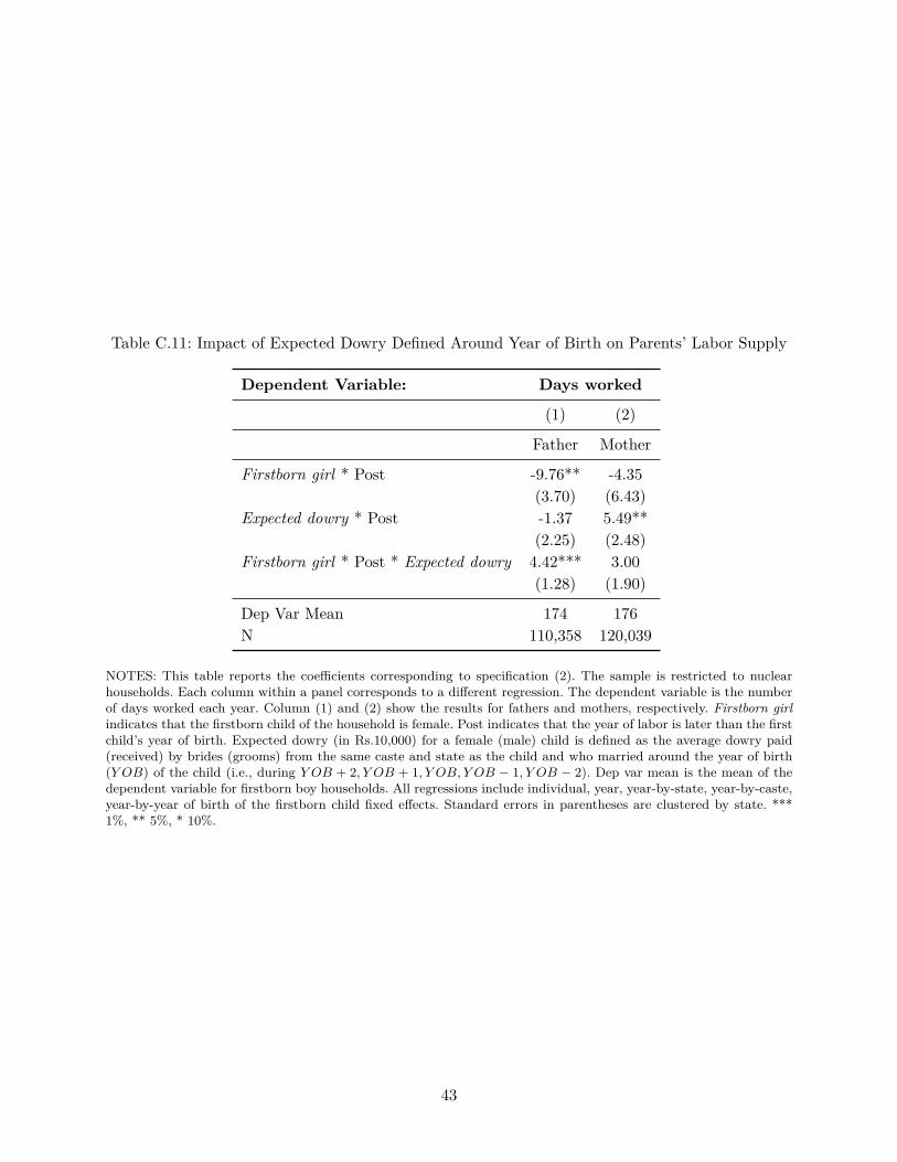
Table C.11: Impact of Expected Dowry Defined Around Year of Birth on Parents’ Labor Supply

Dependent Variable: Days worked

(1) (2)

Father Mother

Firstborn girl * Post -9.76** -4.35(3.70) (6.43)

Expected dowry * Post -1.37 5.49**(2.25) (2.48)

Firstborn girl * Post * Expected dowry 4.42*** 3.00(1.28) (1.90)

Dep Var Mean 174 176N 110,358 120,039

NOTES: This table reports the coefficients corresponding to specification (2). The sample is restricted to nuclearhouseholds. Each column within a panel corresponds to a different regression. The dependent variable is the numberof days worked each year. Column (1) and (2) show the results for fathers and mothers, respectively. Firstborn girlindicates that the firstborn child of the household is female. Post indicates that the year of labor is later than the firstchild’s year of birth. Expected dowry (in Rs.10,000) for a female (male) child is defined as the average dowry paid(received) by brides (grooms) from the same caste and state as the child and who married around the year of birth(Y OB) of the child (i.e., during Y OB + 2, Y OB + 1, Y OB, Y OB − 1, Y OB − 2). Dep var mean is the mean of thedependent variable for firstborn boy households. All regressions include individual, year, year-by-state, year-by-caste,year-by-year of birth of the firstborn child fixed effects. Standard errors in parentheses are clustered by state. ***1%, ** 5%, * 10%.

43

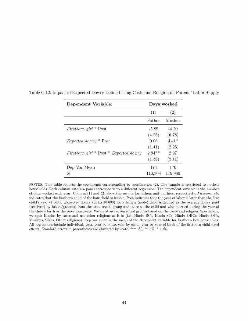
Table C.12: Impact of Expected Dowry Defined using Caste and Religion on Parents’ Labor Supply

Dependent Variable: Days worked

(1) (2)

Father Mother

Firstborn girl * Post -5.89 -4.20(4.25) (6.78)

Expected dowry * Post 0.06 4.41*(1.41) (2.25)

Firstborn girl * Post * Expected dowry 2.94** 2.97(1.38) (2.11)

Dep Var Mean 174 176N 110,308 119,989

NOTES: This table reports the coefficients corresponding to specification (2). The sample is restricted to nuclearhouseholds. Each column within a panel corresponds to a different regression. The dependent variable is the numberof days worked each year. Column (1) and (2) show the results for fathers and mothers, respectively. Firstborn girlindicates that the firstborn child of the household is female. Post indicates that the year of labor is later than the firstchild’s year of birth. Expected dowry (in Rs.10,000) for a female (male) child is defined as the average dowry paid(received) by brides(grooms) from the same social group and state as the child and who married during the year ofthe child’s birth or the prior four years. We construct seven social groups based on the caste and religion. Specifically,we split Hindus by caste and use other religions as it is (i.e., Hindu SCs, Hindu STs, Hindu OBCs, Hindu OCs,Muslims, Sikhs, Other religions). Dep var mean is the mean of the dependent variable for firstborn boy households.All regressions include individual, year, year-by-state, year-by-caste, year-by-year of birth of the firstborn child fixedeffects. Standard errors in parentheses are clustered by state. *** 1%, ** 5%, * 10%.

44