downscaling cokriging for image sharpening - ugrhera.ugr.es/doi/16518524.pdf · downscaling...

ent 102 (2006) 86–98www.elsevier.com/locate/rse

Remote Sensing of Environm

Downscaling cokriging for image sharpening

Eulogio Pardo-Igúzquiza a,⁎, Mario Chica-Olmo a, Peter M. Atkinson b

a Laboratorio de Teledeteccion Geoestadistica y SIG, Departmento de Geodinamica, Campus Fuentenueva s/n, Universidad de Granada, 18091 Granada, Spainb School of Geography, University of Southampton, Highfield, Southampton SO17 1BJ, UK

Received 13 August 2005; received in revised form 3 February 2006; accepted 4 February 2006

Abstract

The main aim of this paper is to show the utility of cokriging for image fusion (i.e. increasing the spatial resolution of satellite sensor images). It isassumed that co-registered images with different spatial and spectral resolutions of the same scene are available and the task is to generate newremote sensing images at the finer spatial resolution for the spectral bands available only at the coarser spatial resolution. The main advantages ofcokriging are that it takes into account the correlation and cross-correlation of images, it accounts for the different supports (i.e. pixel sizes), it cantake into account explicitly the point spread function of the sensor and has the property of prediction coherence. In addition, ancillary images(topographic maps, thematic maps, etc.) as well as sparse experimental data could be included in the process. The main drawback of cokriging in theprevious context is that it requires several covariances and cross-covariances some of which are not accessible empirically (i.e. from the pixel valuesof the images). The solution adopted in this paper was to use linear systems theory to obtain the required covariances from the ones that wereestimated empirically. Cokriging was compared with a benchmark image fusion approach (the high pass filter method) to assess performance againsta standard. In fact, cokriging may be seen as a generalization of the high pass filter method where the low pass filter and high pass filter are estimatedby fitting parameters to data. The present paper discusses the downscaling cokriging method, shows its implementation and illustrates the process inthe case of sharpening several remotely sensed images. The desired target image was known so that the performance of the method could beevaluated realistically. Different statistics were used to show that the cokriged predictions were more precise than the HPF predictions. Downscalingcokriging is a new method of great potential in remote sensing that should be incorporated to the toolkit of the remote sensing researcher.© 2006 Elsevier Inc. All rights reserved.

Keywords: Image enhancement; Remote sensing; Geostatistics; Covariance; Variogram; Cross-variogram; Regularization; Deconvolution; Landsat EnhancedThematic Mapper

1. Introduction

Different satellite sensors acquire information on the Earth'ssurface at different spatial resolutions and for differentwavebands of the electromagnetic spectrum. It has becomeincreasingly common that images from different sensors can beacquired of the same area, and occasionally at reasonablycomparable times and dates. Moreover, several recent platformsprovide data from more than one sensor. A common choice isthe combination of a multispectral sensor in several wavebandswith a relatively coarse spatial resolution, with a panchromaticsensor with a relatively fine spatial resolution. An early example

⁎ Corresponding author.E-mail addresses: [email protected] (E. Pardo-Igúzquiza),

[email protected] (M. Chica-Olmo), [email protected] (P.M. Atkinson).

0034-4257/$ - see front matter © 2006 Elsevier Inc. All rights reserved.doi:10.1016/j.rse.2006.02.014

was the Système Pour Observation de la Terre (SPOT)multispectral sensor with a spatial resolution of 20 m andpanchromatic sensor with a spatial resolution of 10 m. Morerecently, very fine spatial resolution sensors have tended toprovide this same combination of multispectral and panchro-matic images (e.g., IKONOS with multispectral (4 m) andpanchromatic (1 m) imagery and Quickbird with multispectral(2.4 m) and panchromatic (0.6 m) imagery, where the numbersin parentheses indicate spatial resolution).

Given images of the same area produced by sensors ofdifferent spatial and spectral characteristics an obviousobjective is to produce a single image that contains as muchas possible of the information in each original image by somemerging process. In this paper, we consider the terms merging,fusion, integration and combination as synonymous. Imagemerging is a broad subject (see Wald (1999)) and it has beenused for different tasks such as image sharpening, detection of

mailto:[email protected]



http://dx.doi.org/10.1016/j.rse.2006.02.014

87E. Pardo-Igúzquiza et al. / Remote Sensing of Environment 102 (2006) 86–98

temporal changes, replacement of defective data, stereo-vision,etc. (e.g. Pohl & Van Genderen, 1998). In this paper, theobjective is to increase the spatial resolution of a given imagefor a particular spectral band given at least two original images:an image with a coarse spatial resolution for the band of interestand a second image with the desired spatial resolution but of adifferent spectral band. The specific objective then is imagesharpening or image enhancement. Even for the single task ofimage sharpening, a plethora of methods have been proposed:Hue-Intensity-Saturation (HIS) method, principal componentsanalysis (PCA) method, high-pass filter (HPF) method (e.g.Chavez et al., 1991), regression predictor (e.g. Price, 1999),smoothing filter based intensity modulation (e.g. Liu, 2000),wavelet transform and multiscale Kalman filter (e.g. Simone etal., 2002), multiresolution wavelet analysis (e.g. Nuñez et al.,1999) and ARSIS method (e.g. Ranchin et al., 2003) to namejust a few. It is beyond the scope of this paper to review andcompare the above methods.

In the image sharpening objective as defined here, it is ofinterest not only to have a visually pleasant image revealingmore detail, but detail that must relate to real features and not justartifacts (i.e. spurious features). If the task of the sharpeningprocess was just to improve visual quality then the simple HISmethod may be sufficient (as in Pellemans et al., 1993, forexample).

Cokriging has been previously used for image fusion(Memarsadeghi et al., 2005; Nishii et al., 1996) but withouttaking into account the important issue of the effect of differentareal supports (pixel sizes). Area-to-point kriging, whichconsiders the problem of predicting from areal supports topoints, but only for the univariate case, has been considered byKyriakidis (2004) and Kyriakidis and Yoo (2005). In this paper,geostatistical downscaling cokriging, is proposed as a new andtheoretically sound method for image sharpening. In downscal-ing cokriging, the predictor is unbiased and minimizes theprediction variance. It explicitly takes into account pixel sizes,correlations, cross-correlations and the point spread function ofthe sensor. In addition, downscaling cokriging can incorporateinformation provided by ancillary and sparse experimental data.

In increasing the spatial resolution of remote sensing imagesthe downscaling cokriging procedure requires the definition ofcovariances and cross-covariances that are not accessible experi-mentally, and the provision of these functions requires additionalprocessing techniques to be defined. In this paper, we describe apossible solution to the problem of estimating these functionsand, thus, provide a means to fit the cokriging model (i.e., linearmodel of coregionalization) to empirical data. Specifically, thesolution adopted was to use linear systems theory to obtain therequired covariances from those estimated empirically.

The downscaling cokriging method, together with theevaluation of the required covariance and cross-covariancemodels, is described below.

2. Method: downscaling cokriging

Before describing the cokriging system, it is necessary todefine the geostatistical concept of support. The spatial

resolution of a given sensor is approximately equal to the sizeof a pixel in an image provided by that sensor. For example, thespatial resolution of the Landsat Thematic Mapper (TM) sensoris 30 m and that of the Système Pour Observation de la Terre(SPOT) Panchromatic sensor is 10 m. The area of an ob-servation that is assigned to a pixel is known in geostatistics asthe support. In particular, the value assigned to a pixel re-presents the average radiation arriving at the sensor from an areaon the ground equal to the support. The support may beapproximated by, but is not necessarily equal to the pixel,potentially varying in size, geometry and orientation.

The general theory of ordinary cokriging can be found else-where (see Chilès & Delfiner, 1999; Goovaerts, 1997; Journel &Huijbregts, 1978; Isaaks & Srisvastava, 1989; Wackernagel,1995, for the general formulation, and Atkinson et al., 1992,1994, for cokriging in remote sensing). However, in all theprevious references the cokriging system is such that thesupport of the variable to be predicted is equal to or larger thanthe support of the empirical information, while in the problemconsidered here, sharpening of remote sensing images, thesupport of the variable to be predicted is smaller than or equal tothe support of the empirical data. For this reason, and forcompleteness, the cokriging system as applied in the proposedmethod is developed in Appendix A.

The high spatial resolution cokriged image for spectral bandk calculated from a low spatial resolution image (of the spectralband k) and a high spatial resolution image (from a differentspectral band l is given by

Zkuðx0Þ ¼

XNi¼1

k0i ZkV ðxiÞ þ

XMj¼1

b0j ZluðxjÞ ð1Þ

where:

Z uk(x0) random variable (RV) of pixel of areal size u, with

spatial location x0={x1,x2} and spectral band kestimated by cokriging (the circumflex meansestimated)

ZVk (xi) RV of pixel of the low spatial resolution image with

areal size V and spectral band k. N of these pixels areused. For example, N=3×3 window of pixels. Theweight assigned to the random variable of the i-th pixelis λi

0

Zul(xj) RV of pixel of the high spatial resolution image with

areal size u and spectral band l. M of these pixels areused. For example, M=5×5 window of pixels. Theweight assigned to the random variable of the j-th pixelis βj

0

The purpose of cokriging is to obtain the two sets of weights{λi

0; i=1, …, N} and {βj0; j=1, …, M} which are optimal in the

sense of giving an unbiased estimator and with minimumestimation variance. It may be seen how Eq. (1) may beinterpreted as two weighted moving averages of the low spatialresolution and high spatial resolution images. By consideringthe conditions that the weights must fulfil (Eqs. (A10) and(A11) of the Appendix) it may be seen how the cokriging

88 E. Pardo-Igúzquiza et al. / Remote Sensing of Environment 102 (2006) 86–98

amounts to the application of a low pass filter to the low spatialresolution image (first term of the right hand side of Eq. (1)) anda high pass filter to the high spatial resolution image (secondterm of the right hand side of Eq. (1)), and summation of thefiltered images:

Zkuðx0Þ ¼ L½Zk

V ðxiÞ� þ H ½ZluðxjÞ� ð2Þ

where:

L[.] low pass filter operatorH [.] high pass filter operator

The cokriging filters take into account the support effect (i.e.effect of the pixel sizes) and the cross-covariance of the imageswhich implies an implicit interaction between the low pass andhigh pass filters evaluating their relative importance.

The downscaling cokriging approach has a strong connec-tion with the HPF method (Chavez et al., 1991); in fact, bothmethods can be expressed as Eq. (2). However, there is afundamental difference. The weights of the filters in cokrigingare data driven as they are directed by the data (by using thecovariances and cross-covariances) and by minimizing thestatistical criteria of unbiasedness and minimum estimationvariance. In general, the HPF is more ad hoc because the filtersare chosen without reference to the data. For example, the lowpass filter may be provided by resampling the low spatialresolution image using bilinear interpolation and the high passfilter might be a 5×5 Laplacian (Russ, 1999) applied to the highspatial resolution image.

By using the moving window approach in cokriging theprocess is adaptive with respect to variations in the local mean(i.e. non-stationary processes). A procedure that could beimplemented, but that has not been followed here, is to estimatethe variogram locally for different areas. However, the use of aglobal model has the advantage of providing a more statisticallyreliable model. Nishii et al. (1996) report more accurateprediction with a global model, although the results could becase specific. This subject remains open to future research. Thus,in our global approach, the weights (low and high pass filters) arecalculated once. Once the weights are calculated their applicationas a moving window in Eq. (1) for predicting the desired highspatial resolution image is as efficient as the application of anyfilter to an image (a few seconds of computer time).

With respect to point-to-point cokriging, downscalingcokriging presents two new covariance functions in the right-hand side of the cokriging system (i.e. matrix B in Eq. (A17) ofthe Appendix):

CuVkk (s): cross-covariance between the variables Zu

k(x)and ZVk (x).

Cuukl (s): cross-covariance between the variables Zu

k(x)and Zul (x).

The first is a cross-covariance between the same band(number k) but for different supports, while the second is across-covariance between the two bands for the small support u.In both cases, because Zu

k(x) is unknown, they cannot beestimated empirically. However, they can be derived from the

empirical covariances using linear systems theory (Papoulis,1984).

We assume that for any band of the spectrum the pixel valuegives the radiance coming from the ground and averaged for thepoints inside a pixel. Then:

ZkuðxÞ ¼

1juðxÞj

ZuðxÞ

Zk•ðyÞdy ð3Þ

ZkV ðxÞ ¼

1jV ðxÞj

ZV ðxÞ

Zk•ðyÞdy ð4Þ

where

Z•k(y) RF of band k at point spatial resolution (•≪ubV), i.e.

a pixel of infinitesimal size. One can think of this pointimage as a theoretical idealization for implementationof our method, even if that image is difficult to realizephysically.

|A| measure (area) of support A.

The process described in Eqs. (3) and (4) is known in linearsystems theory as an integrated or averaged process while ingeostatistics it is referred to as regularization.

Basically, the integrated process may be seen as a linear systemwhere the input is a point random function (RF) and the output isan averaged (or filtered) value, and can be described as the (two-dimensional) convolution between the point RF and a determin-istic function known as the impulse response of the system. Forexample, the impulse response (or point spread function (PSF))hV(y) for the integrated process given by Eq. (4) is given by:

hV ðyÞ ¼1

V ðxÞ if yaV ðxÞ0 otherwise

8<: ð5Þ

Eqs. (3)–(5) are exact for integrated physical processes likemean rainfall over an area while in remote sensing the situationis, in general, more complicated. The PSF is genarally morecomplex than the one given in Eq. (5). The PSF depends on thesatellite sensor, but in general:

• It is not constant as in Eq. (5) but has larger values around thecentre of the pixel and decreases towards the borders (see, forexample, Cracknell, 1998, where the PSF of the AVHRRsensor is given).

• The point spread function applied to a pixel V (or u) averagesradiance from that pixel and neighbouring pixels.

Then, in general, for a pixel of arbitrary size u:

ZkuðxÞ ¼

ZuðxÞ

Zk•ðyÞhuðyÞdy ð6Þ

with a non-constant impulse-response function hu(y) (for someoptical devices this function looks like a Gaussian probabilitydensity function, but for sensors on satellites it looks more likethe one referred to before in Cracknell, 1998). Then, if a par-ticular form of hu(y) is desired it could be used in the followingcalculations. Nevertheless, for simplicity in the presentation and


to build the experiment presented below, the simple form givenin Eq. (5) will be used.

The results of linear systems theory can be established in thespatial domain or in the frequency domain. However, since theresults of both domains are equivalent, the spatial domain isused to limit the results to spatial covariance functions.

Calculation of CuVkk (s). A well-known result from linear

systems theory is (Journel & Huijbregts, 1978; Matheron, 1962;Papoulis, 1984):

CkkVV ðsÞ ¼ Ckk

••ðsÞ*hV ðsÞ*hV ð−sÞ ð7Þ

where s is the vector representing Euclidean separation.Usually, this expression is simplified by introducing the so-

called deterministic covariance ρ(s) which is equal to:

qV ðsÞ ¼ hV ðsÞ*hV ð−sÞ ð8Þso that

CkkVV ðsÞ ¼ Ckk

••ðsÞ*qV ðsÞ ð9Þwhere

* the convolution operatorC••kk (s) the covariance of the point process Z•

k(x)ρV (s) the deterministic covariance, also known in the

geostatistical literature as the geometric covariogram(Matheron, 1975, 1986)

The covariance C••kk (s) can be calculated from Eq. (9)

because the other two terms in the equation are known. Thisprocess is known as deconvolution (deregularization in thegeostatistical literature) and is achieved by (i) suggestingtentative models of C••

kk (s), which are convolved with thedeterministic covariance ρV (s) and (ii) comparing the resultwith CVV

kk (s). The process continues until the fit is consideredsatisfactory. It is well known that deconvolution is an ill-posedproblem in mathematical terms. That is, its solution is notunique and there could be many forms of the covariance C••

kk (s)which solve Eq. (9). However, we impose some restrictionswhich make the solution, in general, unique:

• We assume a functional form for the covariance C••kk (s)

which is dependent on a few parameters. For example, in theisotropic case two parameters (the variance and the range)are defined for a particular model, for example, spherical.

• For a punctual process Z•k(x), and neglecting measurement

error, a nugget variance is not allowed. This makes perfectphysical sense because a point would be enclosed in aphysical object (of a given size) which is homogeneous orlocally homogeneous and then there is no nugget effect at thepoint level.

Under these reasonable conditions, the solution of Eq. (9)has the following steps:

1. The covariance CVVkk (s) is estimated from the experimental

image ZVk (x) for a finite number of lags L, i.e. the

experimental covariance {ĈVVkk (si); i=1, …, L}. This can be

achieved for different directions to detect possibleanisotropies.

2. In view of the representation of {ĈVVkk (si); i=1, …, L} and

other possible considerations, a basic model with a finitenumber of unknown parameters is chosen for C••

kk (s), thespatial covariance of Z•

k(x). For example, an isotropicspherical model, which has two unknowns {σ2,θ}; thevariance and correlation length or range, respectively.

3. For each pair of parameter values for {σ2,θ} we obtain adifferent model of C••

kk (s). Using Eq. (9), C••kk (s) is convolved

with the deterministic covariance ρV (s), which is known, inorder to provide the solution of the equation which isdenoted as C

∼••kk (s).

4. C∼VVkk (s) is compared with the estimated covariance ĈVV

kk (s)and some measure of misfit is calculated, for example, thesum of squared differences for the L available lags from theestimation.

5. The model selected for C••kk (s) is defined by the pair of

parameter values {σ2,θ} for which the previous measure ofmisfit is minimum.

Once C••kk (s) is estimated we could apply the same previous

result to estimate Cuukk(s) as:

CkkuuðsÞ ¼ Ckk

••ðsÞ*quðsÞ ð10Þ

where the deterministic covariance ρu(s) is defined as in Eq. (8)but using the impulse response hu(s) defined by Eq. (5) with thesupport V replaced by the support u.

Finally, the desired covariance is calculated from anotherwell-known result of linear systems theory (Papoulis, 1984):

CkkuV ðsÞ ¼ Ckk

uuðsÞ*hV ðsÞ ð11Þ

Calculation of Cuuk l (s). This cross-covariance between the two

different bands for the same small support may be calculatedfrom relations similar to the previous ones and starting from:

CklVuðsÞ ¼ Ckl

••ðsÞ*hV ðsÞ*huðsÞ ð12Þ

because CVukl (s) can be inferred from the experimental images.

Next from C••kl (s), Cuu

kl (s) is obtained as in Eq. (9).The previous covariance and cross-covariance may be

isotropic or anisotropic. Even in the isotropic case, althoughthe isotropic covariance (or cross-covariance) is radiallysymmetric, that is not the case for the previous transfer functionsand deterministic covariances for rectangular (and square)pixels. There is an anisotropy between the directions parallelto the pixel sides and diagonally across the pixel. This anisotropyhas already been highlighted by authors working in geostatistics(e.g. Mantoglou & Wilson, 1982). However, in practice, thatanisotropy is negligible and only begins to be worth taking intoaccount when the largest length of the support (allowing forrectangular support) is at least half of the range or correlationlength of the covariance (e.g. Pardo-Iguzquiza, 1991).

14

12

10

8

6

4

2

0

Var

iog

ram

(D

N)^

2

A

0 500 1000Distance (m)

1500 2000

Experimental 0

Visual fitting

14

12

10

8

6

4

2

0

Var

iog

ram

(D

N)^

2

B


1500 2000

Experimental 45

Visual fitting

C14

12

10

8

6

4

2

0

Var

iog

ram

(D

N)^

2


1500 2000

Experimental 90

Visual fitting

D14

12

10

8

6

4

2

0

Var

iog

ram

(D

N)^

2


1500 2000

Experimental 135

Visual fitting

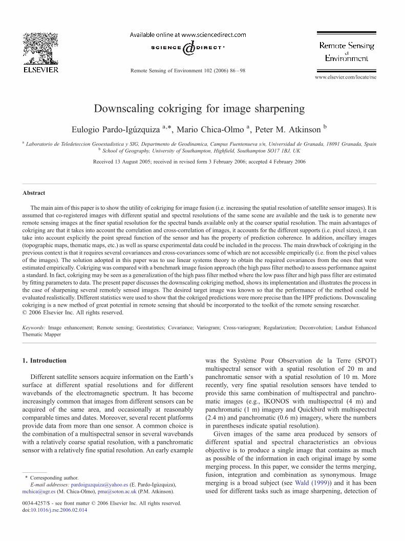
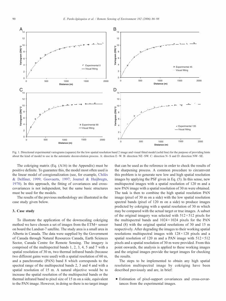
Fig. 1. Directional experimental variograms (squares) for the low spatial resolution band 2 image and visual fitted model (solid line) for the purpose of providing hintsabout the kind of model to use in the automatic deconvolution process. A: direction E–W. B: direction NE–SW. C: direction N–S and D: direction NW–SE.


The cokriging matrix (Eq. (A16) in the Appendix) must bepositive definite. To guarantee this, the model most often used isthe linear model of coregionalization (see, for example, Chilès& Delfiner, 1999; Goovaerts, 1997; Journel & Huijbregts,1978). In this approach, the fitting of covariances and cross-covariances is not independent, but the same basic structuresmust be used for the models.

The results of the previous methodology are illustrated in thecase study given below.

3. Case study

To illustrate the application of the downscaling cokrigingmethod we have chosen a set of images from the ETM+ sensoron board the Landsat-7 satellite. The study area is a small area inAlberta in Canada. The data were supplied by the Governmentof Canada through Natural Resources Canada, Earth SciencesSector, Canada Centre for Remote Sensing. The imagery iscomprised of the multispectral bands 1, 2, 3, 4, 5 and 7 with aspatial resolution of 30 m, two thermal infrared bands (becausetwo different gains were used) with a spatial resolution of 60 m,and a panchromatic (PAN) band 8 which corresponds to thespectral range of the multispectral bands 2, 3 and 4 and with aspatial resolution of 15 m. A natural objective would be toincrease the spatial resolution of the multispectral bands or thethermal infrared band to pixel size of 15 m on a side, equivalentto the PAN image. However, in doing so there is no target image

that can be used as the reference in order to check the results ofthe sharpening process. A common procedure to circumventthis problem is to generate new low and high spatial resolutionimages by applying the PSF given in Eq. (5). In this sense, newmultispectral images with a spatial resolution of 120 m and anew PAN image with a spatial resolution of 30 m were obtained.The task is then to combine the high spatial resolution PANimage (pixel of 30 m on a side) with the low spatial resolutionspectral bands (pixel of 120 m on a side) to produce imagespredicted by cokriging with a spatial resolution of 30 m whichmay be compared with the actual target or true images. A subsetof the original imagery was selected with 512×512 pixels forthe multispectral bands and 1024×1024 pixels for the PANband (8) with the original spatial resolutions of 30 and 15 mrespectively. After degrading the images to their working spatialresolutions multispectral images with 128×128 pixels and aspatial resolution of 120 m and a PAN image with 512×512pixels and a spatial resolution of 30 m were provided. From thispoint onwards, the analysis is applied to these working imagesand the original images provide the target images for checkingthe results.

The steps to be implemented to obtain any high spatialresolution multispectral image by cokriging have beendescribed previously and are, in brief:

• Estimation of pixel-support covariances and cross-covar-iances from the experimental images.

25

20

15

10

5

0

25

20

15

10

5

00 200 400 600 800 1000 1200 1400 1600 1800 2000

0 200 400 600 800 1000 1200 1400 1600 1800 2000

Var

iog

ram

(D

N)^

2V

ario

gra

m (

DN

)^2

Distance (m)

Distance (m)

A

B

Experimental 0

Induced

Experimental 0

Induced

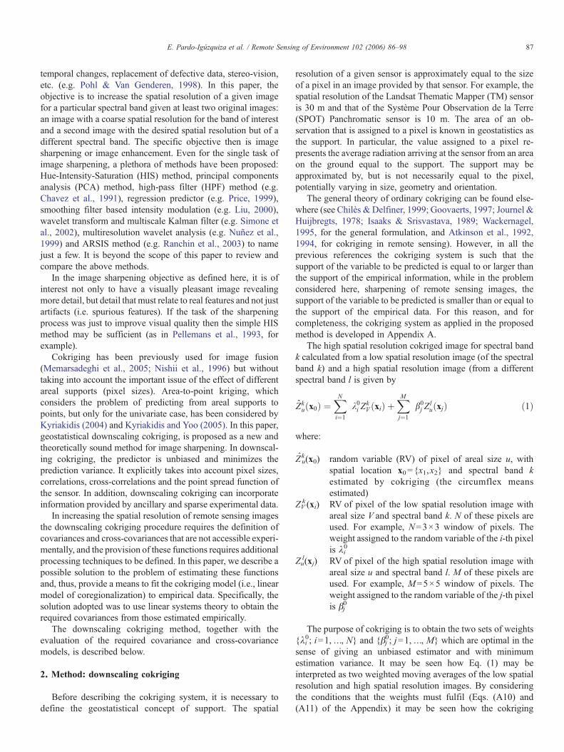
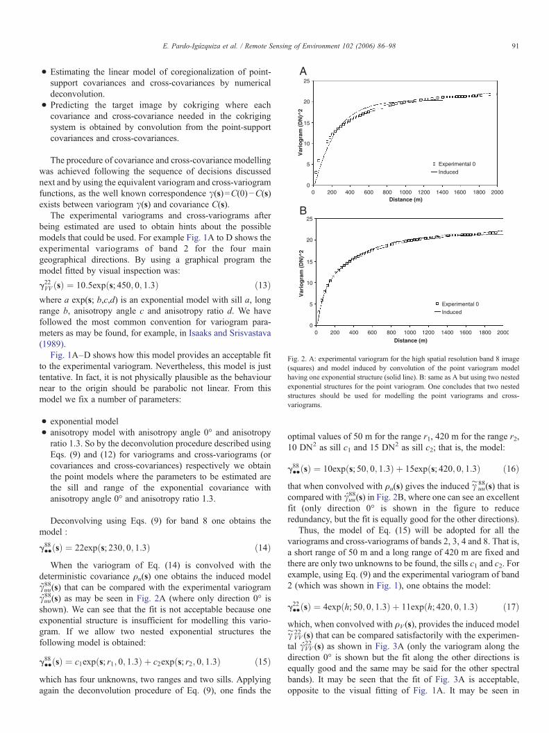
Fig. 2. A: experimental variogram for the high spatial resolution band 8 image(squares) and model induced by convolution of the point variogram modelhaving one exponential structure (solid line). B: same as A but using two nestedexponential structures for the point variogram. One concludes that two nestedstructures should be used for modelling the point variograms and cross-variograms.


• Estimating the linear model of coregionalization of point-support covariances and cross-covariances by numericaldeconvolution.

• Predicting the target image by cokriging where eachcovariance and cross-covariance needed in the cokrigingsystem is obtained by convolution from the point-supportcovariances and cross-covariances.

The procedure of covariance and cross-covariance modellingwas achieved following the sequence of decisions discussednext and by using the equivalent variogram and cross-variogramfunctions, as the well known correspondence γ(s)=C(0)−C(s)exists between variogram γ(s) and covariance C(s).

The experimental variograms and cross-variograms afterbeing estimated are used to obtain hints about the possiblemodels that could be used. For example Fig. 1A to D shows theexperimental variograms of band 2 for the four maingeographical directions. By using a graphical program themodel fitted by visual inspection was:

g22VV ðsÞ ¼ 10:5expðs; 450; 0; 1:3Þ ð13Þwhere a exp(s; b,c,d) is an exponential model with sill a, longrange b, anisotropy angle c and anisotropy ratio d. We havefollowed the most common convention for variogram para-meters as may be found, for example, in Isaaks and Srisvastava(1989).

Fig. 1A–D shows how this model provides an acceptable fitto the experimental variogram. Nevertheless, this model is justtentative. In fact, it is not physically plausible as the behaviournear to the origin should be parabolic not linear. From thismodel we fix a number of parameters:

• exponential model• anisotropy model with anisotropy angle 0° and anisotropyratio 1.3. So by the deconvolution procedure described usingEqs. (9) and (12) for variograms and cross-variograms (orcovariances and cross-covariances) respectively we obtainthe point models where the parameters to be estimated arethe sill and range of the exponential covariance withanisotropy angle 0° and anisotropy ratio 1.3.

Deconvolving using Eqs. (9) for band 8 one obtains themodel :

g88••ðsÞ ¼ 22expðs; 230; 0; 1:3Þ ð14ÞWhen the variogram of Eq. (14) is convolved with the

deterministic covariance ρu(s) one obtains the induced modelγuu88(s) that can be compared with the experimental variogram

γuu88(s) as may be seen in Fig. 2A (where only direction 0° is

shown). We can see that the fit is not acceptable because oneexponential structure is insufficient for modelling this vario-gram. If we allow two nested exponential structures thefollowing model is obtained:

g88••ðsÞ ¼ c1expðs; r1; 0; 1:3Þ þ c2expðs; r2; 0; 1:3Þ ð15Þwhich has four unknowns, two ranges and two sills. Applyingagain the deconvolution procedure of Eq. (9), one finds the

optimal values of 50 m for the range r1, 420 m for the range r2,10 DN2 as sill c1 and 15 DN2 as sill c2; that is, the model:

g88••ðsÞ ¼ 10expðs; 50; 0; 1:3Þ þ 15expðs; 420; 0; 1:3Þ ð16Þthat when convolved with ρu(s) gives the induced γ∼uu

88(s) that iscompared with γuu

88(s) in Fig. 2B, where one can see an excellentfit (only direction 0° is shown in the figure to reduceredundancy, but the fit is equally good for the other directions).

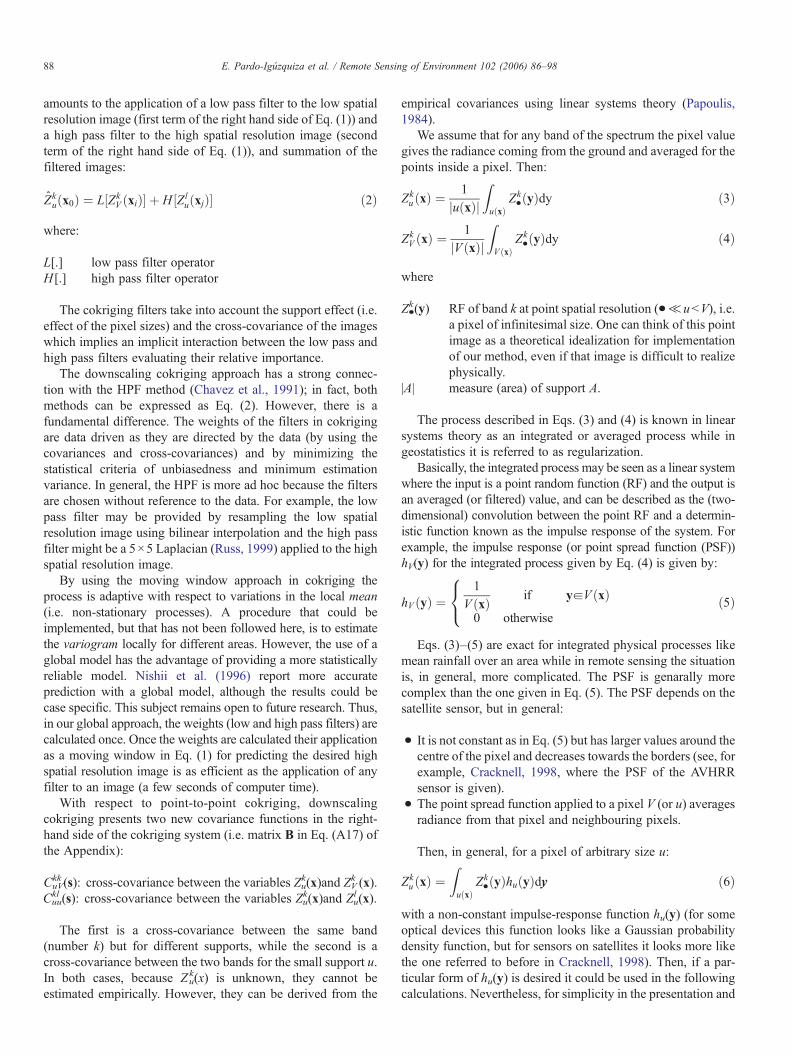
Thus, the model of Eq. (15) will be adopted for all thevariograms and cross-variograms of bands 2, 3, 4 and 8. That is,a short range of 50 m and a long range of 420 m are fixed andthere are only two unknowns to be found, the sills c1 and c2. Forexample, using Eq. (9) and the experimental variogram of band2 (which was shown in Fig. 1), one obtains the model:

g22••ðsÞ ¼ 4expðh; 50; 0; 1:3Þ þ 11expðh; 420; 0; 1:3Þ ð17Þwhich, when convolved with ρV (s), provides the induced modelγ∼VV22 (s) that can be compared satisfactorily with the experimen-

tal γVV22 (s) as shown in Fig. 3A (only the variogram along the

direction 0° is shown but the fit along the other directions isequally good and the same may be said for the other spectralbands). It may be seen that the fit of Fig. 3A is acceptable,opposite to the visual fitting of Fig. 1A. It may be seen in

14

12

10

8

6

4

2

00 500

0 200 400 600 800 1000 1200 1400 1600 1800 2000

1000

Var

iog

ram

(D

N)^

2

14

16

12

10

8

6

4

2

0

Var

iog

ram

(D

N)^

2

Distance (m)

Distance (m)

1500 2000

Experimental 0

Induced

Experimental 0

Induced

A

B

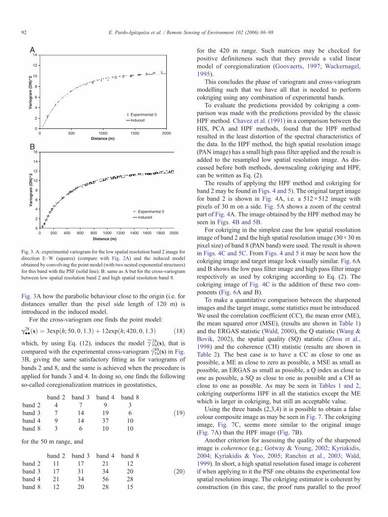
Fig. 3. A: experimental variogram for the low spatial resolution band 2 image fordirection E–W (squares) (compare with Fig. 2A) and the induced modelobtained by convolving the point model (with two nested exponential structures)for this band with the PSF (solid line). B: same as A but for the cross-variogrambetween low spatial resolution band 2 and high spatial resolution band 8.


Fig. 3A how the parabolic behaviour close to the origin (i.e. fordistances smaller than the pixel side length of 120 m) isintroduced in the induced model.

For the cross-variogram one finds the point model:

g28••ðsÞ ¼ 3expðh; 50; 0; 1:3Þ þ 12expðh; 420; 0; 1:3Þ ð18Þwhich, by using Eq. (12), induces the model γ∼Vu

28(s), that iscompared with the experimental cross-variogram γVu

88(s) in Fig.3B, giving the same satisfactory fitting as for variograms ofbands 2 and 8, and the same is achieved when the procedure isapplied for bands 3 and 4. In doing so, one finds the followingso-called coregionalization matrices in geostatistics,

band 2 band 3 band 4 band 8band 2 4 7 9 3band 3 7 14 19 6band 4 9 14 37 10band 8 3 6 10 10

ð19Þ

for the 50 m range, and

band 2 band 3 band 4 band 8band 2 11 17 21 12band 3 17 31 34 20band 4 21 34 56 28band 8 12 20 28 15

ð20Þ

for the 420 m range. Such matrices may be checked forpositive definiteness such that they provide a valid linearmodel of coregionalization (Goovaerts, 1997; Wackernagel,1995).

This concludes the phase of variogram and cross-variogrammodelling such that we have all that is needed to performcokriging using any combination of experimental bands.

To evaluate the predictions provided by cokriging a com-parison was made with the predictions provided by the classicHPF method. Chavez et al. (1991) in a comparison between theHIS, PCA and HPF methods, found that the HPF methodresulted in the least distortion of the spectral characteristics ofthe data. In the HPF method, the high spatial resolution image(PAN image) has a small high pass filter applied and the result isadded to the resampled low spatial resolution image. As dis-cussed before both methods, downscaling cokriging and HPF,can be written as Eq. (2).

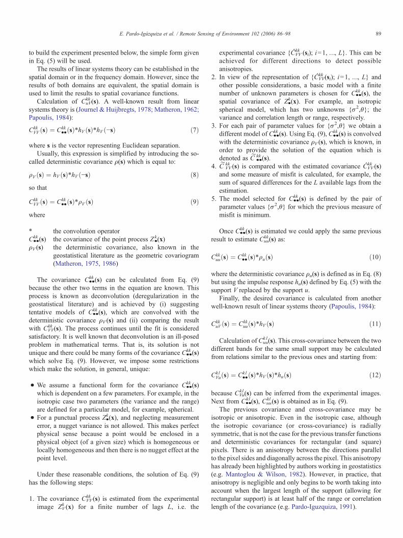
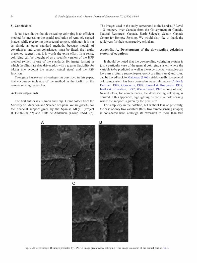
The results of applying the HPF method and cokriging forband 2 may be found in Figs. 4 and 5). The original target imagefor band 2 is shown in Fig. 4A, i.e. a 512×512 image withpixels of 30 m on a side. Fig. 5A shows a zoom of the centralpart of Fig. 4A. The image obtained by the HPF method may beseen in Figs. 4B and 5B.

For cokriging in the simplest case the low spatial resolutionimage of band 2 and the high spatial resolution image (30×30 mpixel size) of band 8 (PAN band) were used. The result is shownin Figs. 4C and 5C. From Figs. 4 and 5 it may be seen how thecokriging image and target image look visually similar. Fig. 6Aand B shows the low pass filter image and high pass filter imagerespectively as used by cokriging according to Eq. (2). Thecokriging image of Fig. 4C is the addition of these two com-ponents (Fig. 6A and B).

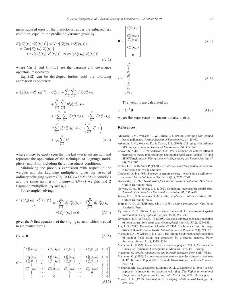
To make a quantitative comparison between the sharpenedimages and the target image, some statistics must be introduced.We used the correlation coefficient (CC), the mean error (ME),the mean squared error (MSE), (results are shown in Table 1)and the ERGAS statistic (Wald, 2000), the Q statistic (Wang &Bovik, 2002), the spatial quality (SQ) statistic (Zhou et al.,1998) and the coherence (CH) statistic (results are shown inTable 2). The best case is to have a CC as close to one aspossible, a ME as close to zero as possible, a MSE as small aspossible, an ERGAS as small as possible, a Q index as close toone as possible, a SQ as close to one as possible and a CH asclose to one as possible. As may be seen in Tables 1 and 2,cokriging outperforms HPF in all the statistics except the MEwhich is larger in cokriging, but still an acceptable value.

Using the three bands (2,3,4) it is possible to obtain a falsecolour composite image as may be seen in Fig. 7. The cokrigingimage, Fig. 7C, seems more similar to the original image(Fig. 7A) than the HPF image (Fig. 7B).

Another criterion for assessing the quality of the sharpenedimage is coherence (e.g.; Gotway & Young, 2002; Kyriakidis,2004; Kyriakidis & Yoo, 2005; Ranchin et al., 2003; Wald,1999). In short, a high spatial resolution fused image is coherentif when applying to it the PSF one obtains the experimental lowspatial resolution image. The cokriging estimator is coherent byconstruction (in this case, the proof runs parallel to the proof

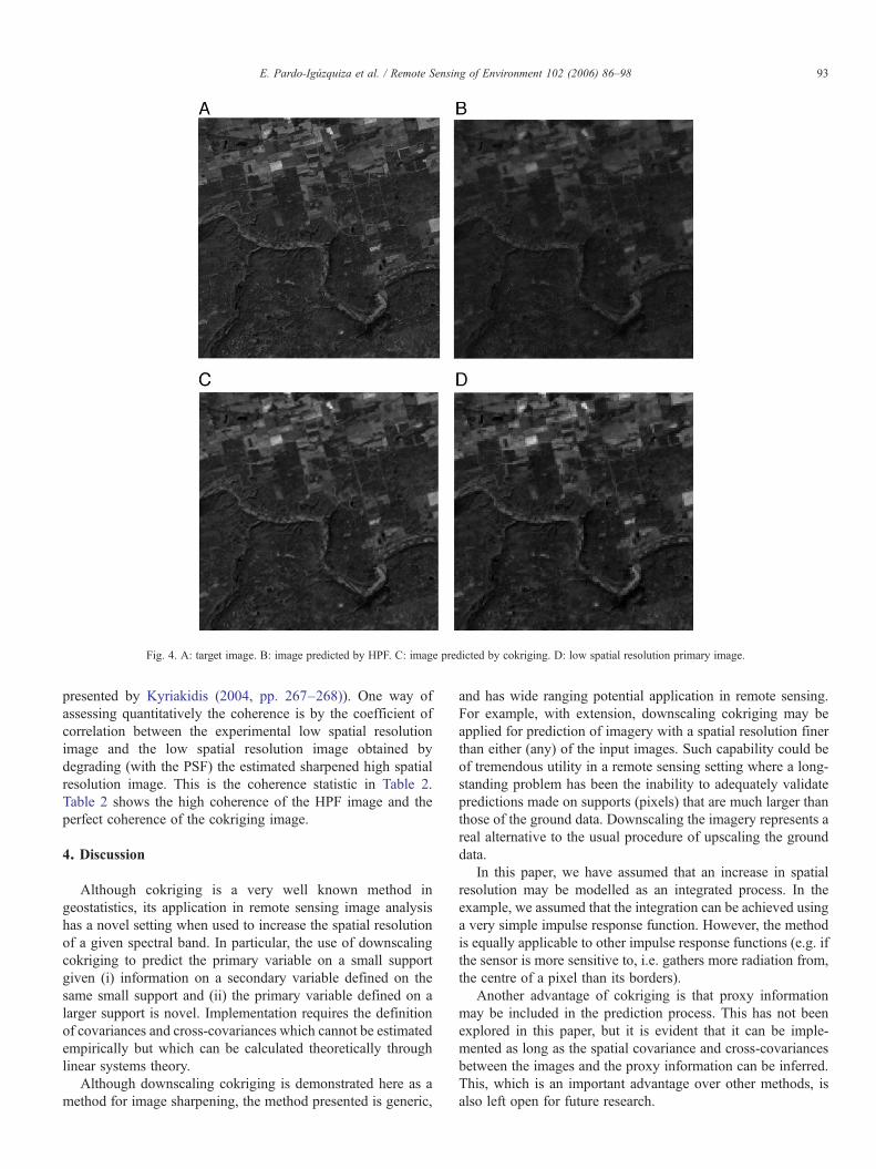
Fig. 4. A: target image. B: image predicted by HPF. C: image predicted by cokriging. D: low spatial resolution primary image.


presented by Kyriakidis (2004, pp. 267–268)). One way ofassessing quantitatively the coherence is by the coefficient ofcorrelation between the experimental low spatial resolutionimage and the low spatial resolution image obtained bydegrading (with the PSF) the estimated sharpened high spatialresolution image. This is the coherence statistic in Table 2.Table 2 shows the high coherence of the HPF image and theperfect coherence of the cokriging image.

4. Discussion

Although cokriging is a very well known method ingeostatistics, its application in remote sensing image analysishas a novel setting when used to increase the spatial resolutionof a given spectral band. In particular, the use of downscalingcokriging to predict the primary variable on a small supportgiven (i) information on a secondary variable defined on thesame small support and (ii) the primary variable defined on alarger support is novel. Implementation requires the definitionof covariances and cross-covariances which cannot be estimatedempirically but which can be calculated theoretically throughlinear systems theory.

Although downscaling cokriging is demonstrated here as amethod for image sharpening, the method presented is generic,

and has wide ranging potential application in remote sensing.For example, with extension, downscaling cokriging may beapplied for prediction of imagery with a spatial resolution finerthan either (any) of the input images. Such capability could beof tremendous utility in a remote sensing setting where a long-standing problem has been the inability to adequately validatepredictions made on supports (pixels) that are much larger thanthose of the ground data. Downscaling the imagery represents areal alternative to the usual procedure of upscaling the grounddata.

In this paper, we have assumed that an increase in spatialresolution may be modelled as an integrated process. In theexample, we assumed that the integration can be achieved usinga very simple impulse response function. However, the methodis equally applicable to other impulse response functions (e.g. ifthe sensor is more sensitive to, i.e. gathers more radiation from,the centre of a pixel than its borders).

Another advantage of cokriging is that proxy informationmay be included in the prediction process. This has not beenexplored in this paper, but it is evident that it can be imple-mented as long as the spatial covariance and cross-covariancesbetween the images and the proxy information can be inferred.This, which is an important advantage over other methods, isalso left open for future research.


5. Conclusions

It has been shown that downscaling cokriging is an efficientmethod for increasing the spatial resolution of remotely sensedimages while preserving the spectral content. Although it is notas simple as other standard methods, because models ofcovariances and cross-covariances must be fitted, the resultspresented suggest that it is worth the extra effort. In a sense,cokriging can be thought of as a specific version of the HPFmethod (which is one of the standards for image fusion) inwhich the filters are data driven plus with a greater flexibility fortaking into account the support (pixel sizes) and the PSFfunction.

Cokriging has several advantages, as described in this paper,that encourage inclusion of the method in the toolkit of theremote sensing researcher.

Acknowledgements

The first author is a Ramon and Cajal Grant holder from theMinistry of Education and Science of Spain. We are grateful forthe financial support given by the Spanish MCyT (ProjectBTE2002-00152) and Junta de Andalucía (Group RNM122).

Fig. 5. A: target image. B: image predicted by HPF. C: image predicte

The images used in the study correspond to the Landsat 7 Level1-G imagery over Canada from the Government of Canada,Natural Resources Canada, Earth Sciences Sector, CanadaCentre for Remote Sensing. We would also like to thank thereviewers for their constructive criticism.

Appendix A. Development of the downscaling cokrigingsystem of equations

It should be noted that the downscaling cokriging system isjust a particular case of the general cokriging system where thevariable to be predicted as well as the experimental variables canhave any arbitrary support (quasi-point or a finite area) and, thus,can be traced back toMatheron (1962). Additionally, the generalcokriging system has been derived in many references (Chilès &Delfiner, 1999; Goovaerts, 1997; Journel & Huijbregts, 1978;Isaaks & Srivastava, 1992; Wackernagel, 1995 among others).Nevertheless, for completeness, the downscaling cokriging isderived in this appendix, highlighting its use in remote sensingwhere the support is given by the pixel size.

For simplicity in the notation, but without loss of generality,the case of only two variables (thus, two remote sensing images)is considered here, although its extension to more than two

d by cokriging. This image is a zoom of the central part of Fig. 5.

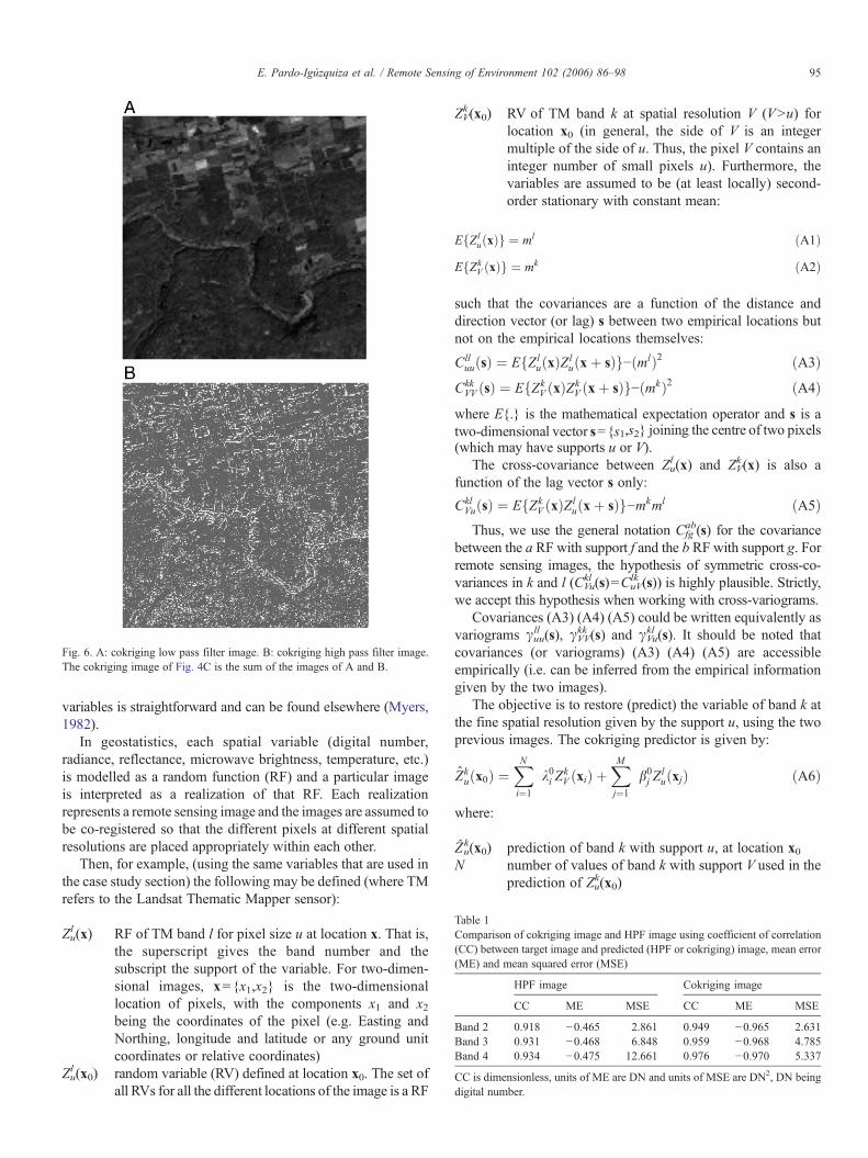
Fig. 6. A: cokriging low pass filter image. B: cokriging high pass filter image.The cokriging image of Fig. 4C is the sum of the images of A and B.

Table 1Comparison of cokriging image and HPF image using coefficient of correlation(CC) between target image and predicted (HPF or cokriging) image, mean error(ME) and mean squared error (MSE)

HPF image Cokriging image

CC ME MSE CC ME MSE

Band 2 0.918 −0.465 2.861 0.949 −0.965 2.631Band 3 0.931 −0.468 6.848 0.959 −0.968 4.785Band 4 0.934 −0.475 12.661 0.976 −0.970 5.337

CC is dimensionless, units of ME are DN and units of MSE are DN2, DN beingdigital number.


variables is straightforward and can be found elsewhere (Myers,1982).

In geostatistics, each spatial variable (digital number,radiance, reflectance, microwave brightness, temperature, etc.)is modelled as a random function (RF) and a particular imageis interpreted as a realization of that RF. Each realizationrepresents a remote sensing image and the images are assumed tobe co-registered so that the different pixels at different spatialresolutions are placed appropriately within each other.

Then, for example, (using the same variables that are used inthe case study section) the following may be defined (where TMrefers to the Landsat Thematic Mapper sensor):

Zul (x) RF of TM band l for pixel size u at location x. That is,

the superscript gives the band number and thesubscript the support of the variable. For two-dimen-sional images, x={x1,x2} is the two-dimensionallocation of pixels, with the components x1 and x2being the coordinates of the pixel (e.g. Easting andNorthing, longitude and latitude or any ground unitcoordinates or relative coordinates)

Zul (x0) random variable (RV) defined at location x0. The set of

all RVs for all the different locations of the image is a RF

ZVk (x0) RV of TM band k at spatial resolution V (VNu) for

location x0 (in general, the side of V is an integermultiple of the side of u. Thus, the pixel V contains aninteger number of small pixels u). Furthermore, thevariables are assumed to be (at least locally) second-order stationary with constant mean:

EfZluðxÞg ¼ ml ðA1Þ

EfZkV ðxÞg ¼ mk ðA2Þ

such that the covariances are a function of the distance anddirection vector (or lag) s between two empirical locations butnot on the empirical locations themselves:

ClluuðsÞ ¼ EfZl

uðxÞZluðxþ sÞg−ðmlÞ2 ðA3Þ

CkkVV ðsÞ ¼ EfZk

V ðxÞZkV ðxþ sÞg−ðmkÞ2 ðA4Þ

where E{.} is the mathematical expectation operator and s is atwo-dimensional vector s={s1,s2} joining the centre of two pixels(which may have supports u or V).

The cross-covariance between Zul (x) and ZV

k (x) is also afunction of the lag vector s only:

CklVuðsÞ ¼ EfZk

V ðxÞZluðxþ sÞg−mkml ðA5Þ

Thus, we use the general notation Cfgab(s) for the covariance

between the a RF with support f and the b RF with support g. Forremote sensing images, the hypothesis of symmetric cross-co-variances in k and l (CVu

kl (s)=CuVlk (s)) is highly plausible. Strictly,

we accept this hypothesis when working with cross-variograms.Covariances (A3) (A4) (A5) could be written equivalently as

variograms γuull (s), γVV

kk (s) and γVukl (s). It should be noted that

covariances (or variograms) (A3) (A4) (A5) are accessibleempirically (i.e. can be inferred from the empirical informationgiven by the two images).

The objective is to restore (predict) the variable of band k atthe fine spatial resolution given by the support u, using the twoprevious images. The cokriging predictor is given by:

Zkuðx0Þ ¼

XNi¼1

k0i ZkV ðxiÞ þ

XMj¼1

b0j ZluðxjÞ ðA6Þ

where:

Zuk(x0) prediction of band k with support u, at location x0

N number of values of band k with support V used in theprediction of Zu

k(x0)

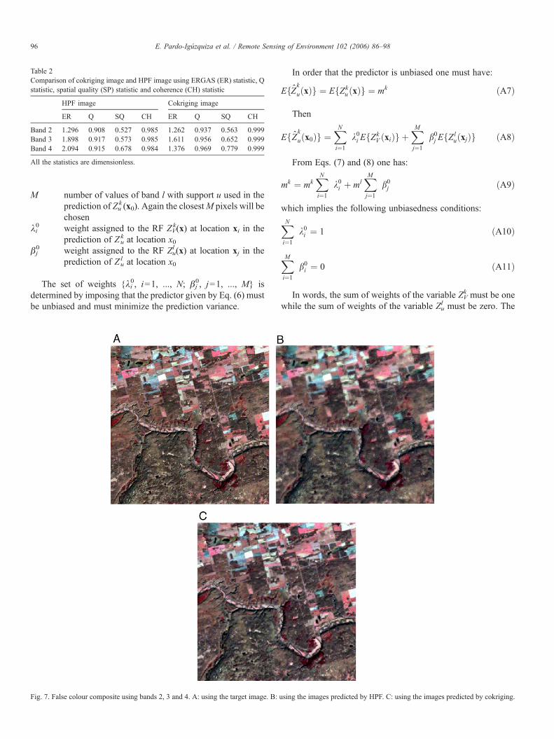
Table 2Comparison of cokriging image and HPF image using ERGAS (ER) statistic, Qstatistic, spatial quality (SP) statistic and coherence (CH) statistic

HPF image Cokriging image

ER Q SQ CH ER Q SQ CH

Band 2 1.296 0.908 0.527 0.985 1.262 0.937 0.563 0.999Band 3 1.898 0.917 0.573 0.985 1.611 0.956 0.652 0.999Band 4 2.094 0.915 0.678 0.984 1.376 0.969 0.779 0.999

All the statistics are dimensionless.


M number of values of band l with support u used in theprediction of Zu

k (x0). Again the closestM pixels will bechosen

λi0 weight assigned to the RF ZV

k(x) at location xi in theprediction of Zu

k at location x0β j0 weight assigned to the RF Zu

l (x) at location xj in theprediction of Zu

l at location x0

The set of weights {λi0, i=1, ..., N; β j

0, j=1, ..., M} isdetermined by imposing that the predictor given by Eq. (6) mustbe unbiased and must minimize the prediction variance.

Fig. 7. False colour composite using bands 2, 3 and 4. A: using the target image. B:

In order that the predictor is unbiased one must have:

EfZk

uðxÞg ¼ EfZkuðxÞg ¼ mk ðA7Þ

Then

EfZk

uðx0Þg ¼XNi¼1

k0i EfZkV ðxiÞg þ

XMj¼1

b0j EfZluðxjÞg ðA8Þ

From Eqs. (7) and (8) one has:

mk ¼ mkXNi¼1

k0i þ mlXMj¼1

b0j ðA9Þ

which implies the following unbiasedness conditions:

XNi¼1

k0i ¼ 1 ðA10Þ

XMi¼1

b0i ¼ 0 ðA11Þ

In words, the sum of weights of the variable ZVk must be one

while the sum of weights of the variable Zul must be zero. The

using the images predicted by HPF. C: using the images predicted by cokriging.


mean squared error of the predictor is, under the unbiasednesscondition, equal to the prediction variance given by:

EfðZ kuðx0Þ−Zk

uðx0ÞÞ2g ¼ VarfðZ kuðx0Þ−Zk

uðx0ÞÞg¼ CovfZk

uðx0Þ;Zkuðx0Þg

þ CovfðZ kuðx0Þ;Zk

uðx0ÞÞg−2CovfðZ kuðx0Þ; Zk

uðx0ÞÞgðA12Þ

where Var{.} and Cov{.,.} are the variance and covarianceoperators, respectively.

Eq. (12) can be developed further until the followingexpression is obtained:

EfðZ kuðx0Þ−Zk

uðx0ÞÞ2g ¼ Ckkuuð0Þ þ

XNi¼1

XNj¼1

k0i k0j C

kkVV ðsijÞ

þXMi¼1

XMj¼1

b0i b0j C

lluuðsijÞ

þ 2XNi¼1

XMj¼1

k0i b0j C

klVuðsijÞ−2

XNi¼1

k0i CkkuV ðs0iÞ

−2XMj¼1

b0j Ckluuðs0jÞ þ 2l1

XNi¼1

k0i −1

!

þ 2l2XNj¼1

b0j ðA13Þ

where it may be easily seen that the last two terms are null andrepresent the application of the technique of Lagrange multi-pliers (μ1,μ2) for including the unbiasedness conditions.

Minimizing the previous expression with respect to theweights and the Lagrange multipliers, gives the so-calledordinary cokriging system (Eq. (A14)) with N+M+2 equationsand the same number of unknowns (N+M weights and 2Lagrange multipliers, μ1 and μ2).

For example, solving:

BEfðZ kuðx0Þ−Zk

uðx0ÞÞ2gBki

¼ 2XNj¼1

k0j CkkVV ðsijÞ þ 2

XMj¼1

b0j CklVuðs1jÞ

−2CkkuV ðs0iÞ ¼ 0 ðA14Þ

gives the N first equations of the kriging system, which is equalto (in matrix form):

Ck ¼ B ðA15Þ

C ¼

CkkVV ðs11Þ : : : Ckk

VV ðs1N Þ CklVuðs11Þ : : : Ckl

Vuðs1M Þ 1 0v O v v O v v

CkkVV ðsN1Þ : : : Ckk

VV ðsNN Þ CklVuðsN1Þ : : : Ckl

VuðsNM Þ 1 0ClkuV ðs11Þ : : : Clk

uV ðs1N Þ Clluuðs11Þ : : : Cll

uuðs1M Þ 0 1v O v v O v v v

ClkuV ðsM1Þ : : : Clk

uV ðsMN Þ ClluuðsM1Þ : : : Cll

uuðsMM Þ 0 11 : : : 1 0 : : : 0 0 00 : : : 0 1 : : : 1 0 0

266666666664

377777777775

ðA16Þ

B ¼

CkkuV ðs01Þv

CkkuV ðs0N ÞCkluuðs01Þv

Ckluuðs0M Þ10

266666666664

377777777775

ðA17Þ

k ¼

k01vk0Nb01v

b0Ml1l2

266666666664

377777777775

ðA18Þ

The weights are calculated as:

k ¼ C−1B ðA19Þwhere the superscript −1 means inverse matrix.

References

Atkinson, P. M., Webster, R., & Curran, P. J. (1992). Cokriging with groundbased radiometry. Remote Sensing of Environment, 41, 45−60.

Atkinson, P. M., Webster, R., & Curran, P. J. (1994). Cokriging with airborneMSS imagery. Remote Sensing of Environment, 50, 335−345.

Chavez, S., Sides, S. C., & Anderson, J. A. (1991). Comparison of three differentmethods to merge multiresolution and multispectral data: Landsat TM andSPOTPanchromatic.Photogrammetric Engineering and Remote Sensing, 57(3), 295−303.

Chilès, J. -P., & Delfiner, P. (1999). Geostatistics: modelling spatial uncertainty.NewYork: John Wiley and Sons.

Cracknell, A. P. (1998). Synergy in remote sensing—what's in a pixel? Inter-national Journal of Remote Sensing, 19(11), 2025−2047.

Goovaerts, P. (1997). Geostatistics for natural resources evaluation. New York:Oxford University Press.

Gotway, C. A., & Young, J. J. (2002). Combining incompatible spatial data.Journal of the American Statistical Association, 97, 632−648.

Isaaks, E. H., & Srisvastava, R. M. (1989). Applied geostatistics. Oxford, UK:Oxford University Press.

Journel, A. G., & Huijbregts, Ch. J. (1978). Mining geostatistics. New-York:Academic Press.

Kyriakidis, P. C. (2004). A geostatistical framework for area-to-point spatialinterpolation. Geographical Analysis, 36(3), 259−289.

Kyriakidis, P. C., & Yoo, E. -H. (2005). Geostatistical prediction and simulationof point values from areal data. Geographical Analysis, 37(2), 124−151.

Liu, J. G. (2000). Evaluation of Landsat-7 ETM+Panchromatic band for imagefusion with multispectral bands. Natural Resources Research, 9(4), 269−276.

Mantoglou, A., &Wilson, J. L. (1982). The turning bands method for simulationof random fields using line generation by a spectral method. WaterResources Research, 18, 1379−1394.

Matheron, G. (1962). Traité de Géostatistique appliquée: Vol. 1, Mémoires duBureau de Recherches Géologiques et Minières, Paris, Ed. Technip.

Matheron, G. (1975). Random sets and integral geometry. New York: Wiley.Matheron, G. (1986). Le covariogramme géometrique des compacts convexes

de R2. Technical Report 2/86. Centre de Géostatistique. Ecole des Mines deParis, 54.

Memarsadeghi, N., Le Moigne, J., Mount, D. M., & Morisette, J. (2005). A newapproach to image fusion based on cokriging. The Eighth InternationalConference on Information Fusion, July, 25–29, PA, USA: Philadelphia.

Myers, D. E. (1982). Formulation of cokriging. Mathematical Geology, 14,249−257.


Nishii, R., Kusanobu, S., & Tanaka, S. (1996). Enhancement of low spatialresolution image based on high resolution bands. IEEE Transactions onGeoscience and Remote Sensing, 34(5), 1151−1158.

Nuñez, J., Otazu, X., Fors, O., Prades, A., Pala, V., & Arbiol, R. (1999).Multiresolution-based image fusion with additive wavelet decomposition.IEEE Transactions on Geoscience and Remote Sensing, 37(3), 1204−1211.

Papoulis, A. (1984). Probability, random variables and stochastic processes,2nd edition. Singapore: McGraw-Hill International Editions.

Pardo-Iguzquiza, E. (1991). Geostatistical simulation of geological variables byspectral methods. PhD dissertation, Department of Geodynamics, Universityof Granada, (p. 412, in Spanish).

Pellemans, A. H. J. M., Jordans, R. W., & Allewijn, R. (1993). Merging multi-spectral and panchromatic SPOT images with respect to the radiometricproperties of the sensor. Photogrammetric Engineering and Remote Sensing,59(1), 81−87.

Pohl, C., & VanGenderen, J. L. (1998). Multisensor image fusion in remotesensing: concepts, methods and applications. International Journal ofRemote Sensing, 19(5), 823−854.

Price, J. C. (1999). Combining multispectral data of different spatial resolution.IEEE Transactions on Geosciences and Remote Sensing, 37(3), 1199−1203.

Russ, J. C. (1999). The image processing handbook, Third edition. Boca Raton(FL): CRC Press.

Simone, G., Farina, A., Morabito, F. C., Serpico, S. B., & Bruzzone, L. (2002).Image fusion techniques for remote sensing applications. InformationFusion, 2, 3−15.

Ranchin, T., Aiazzi, B., Alparone, L., Baronti, S., & Wald, L. (2003). Imagefusion—The ARSIS concept and some successful implementation schemes.Photogrammetry and Remote Sensing, 58, 4−18.

Wackernagel, H. (1995). Multivariate geostatistics. Berlin: Springer.Wald, L. (1999). Some terms of reference in data fusion. IEEE Transactions on

Geoscience and Remote Sensing, 37(3), 1190−1193.Wald, L. (2000). Quality of high resolution synthesized images: is there a simple

criterion? International Conference on Fusion of Earth Data, France Nice,France: SEE GréCA.

Wang, Z., & Bovik, A. C. (2002). A universal image quality index. IEEE SignalProcessing Letters, 9(3), 81−84.

Zhou, J., Civco, D. L., & Silander, J. A. (1998). Awavelet transform method tomerge Landsat TM and SPOT panchromatic data. International Journal ofRemote Sensing, 19(4), 743−757.

downscaling cokriging for image sharpening - ugrhera.ugr.es/doi/16518524.pdf · downscaling...

Documents