What Sculpts What Sculpts the Interstellar the Interstellar
Medium?Medium?
Alyssa A. Goodman
Harvard University
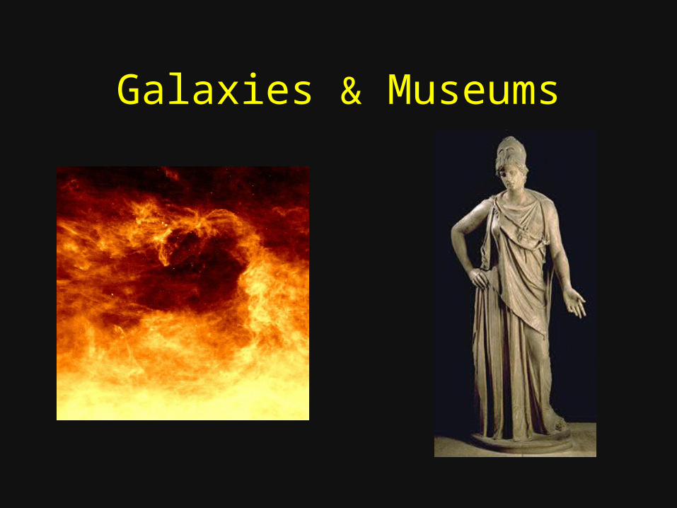
Galaxies & Museums
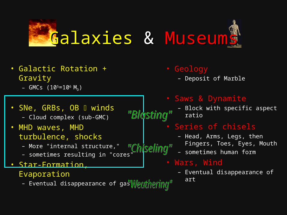
Galaxies Galaxies && MuseumsMuseums
• Galactic Rotation + Gravity– GMCs (105=106 MD)
• SNe, GRBs, OB winds– Cloud complex (sub-GMC)
• MHD waves, MHD turbulence, shocks– More "internal structure," – sometimes resulting in "cores"
• Star-Formation, Evaporation– Eventual disappearance of gas
• Geology– Deposit of Marble
• Saws & Dynamite– Block with specific aspect ratio
• Series of chisels– Head, Arms, Legs, then
Fingers, Toes, Eyes, Mouth– sometimes human form
• Wars, Wind– Eventual disappearance of art
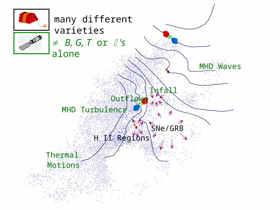
Outflows
MHD Waves
Thermal Motions
MHD Turbulence
Infall
SNe/GRBH II Regions
B, G, T or 's alone
many different varieties
Tools for finding the toolsTools for finding the tools
Key Method:Key Method: Use the velocity field– third (really fourth) dimension– valuable information on energetics
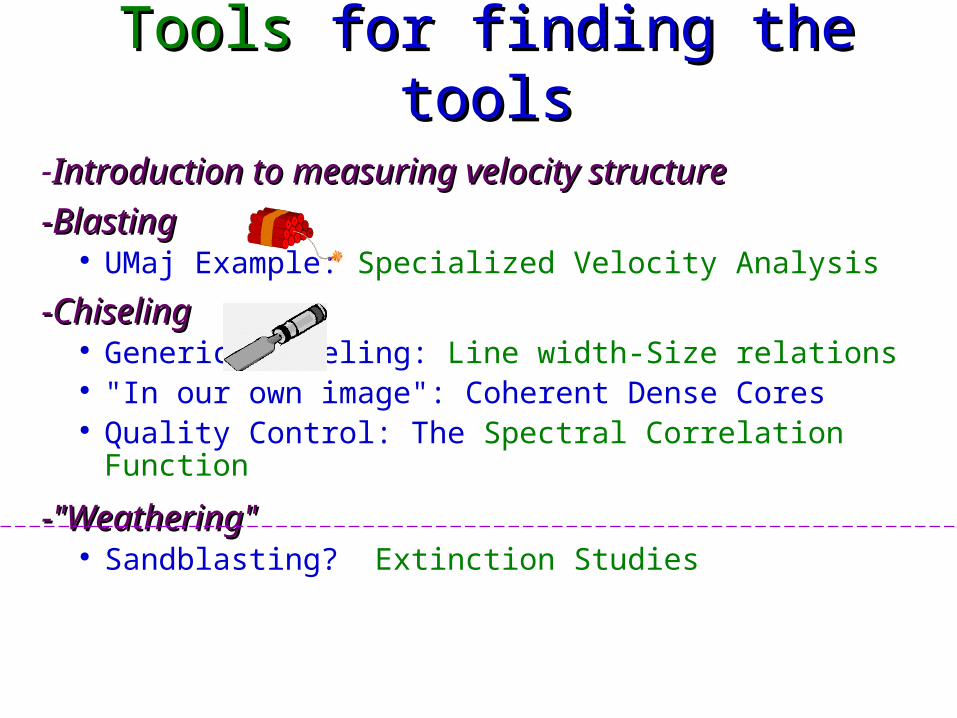
ToolsTools for finding the tools for finding the tools
-Introduction to measuring velocity structureIntroduction to measuring velocity structure
-Blasting-Blasting UMaj Example: Specialized Velocity Analysis
-Chiseling-Chiseling Generic chiseling: Line width-Size relations "In our own image": Coherent Dense Cores Quality Control: The Spectral Correlation Function
-"Weathering"-"Weathering" Sandblasting? Extinction Studies
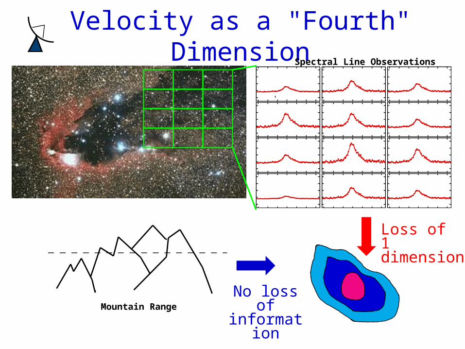
Velocity as a "Fourth" DimensionSpectral Line Observations
Mountain RangeNo loss of
information
Loss of1 dimension
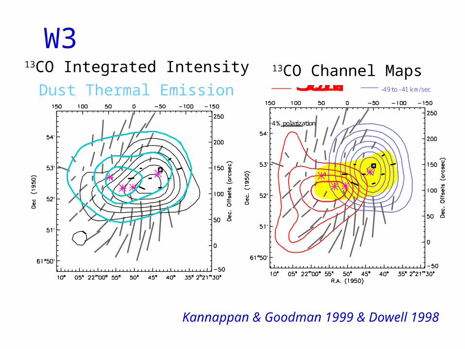
W3
-49 to -41 km/sec-39to-31km/sec
Kannappan & Goodman 1999 & Dowell 1998
o4% polarizati n
13CO Channel Maps13CO Integrated Intensity
Dust Thermal Emission
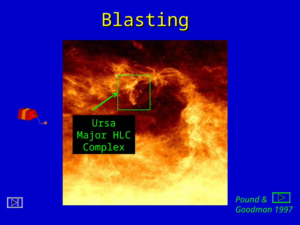
BlastingBlasting
Pound & Goodman 1997
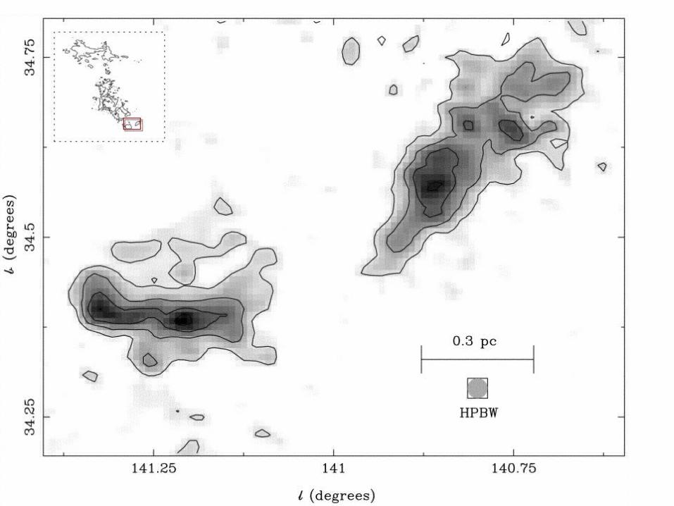
Ursa Major HLC
Complex

• “High-latitude”= very nearbyvery nearby (DUMAJ~100 pc)
• ~No star formation~No star formation1
• Energy distribution very differentEnergy distribution very different than star-forming regions
High Latitude CloudHigh Latitude Cloud2
Gravitational << Magnetic ≈ Kinetic
Star-Forming CloudStar-Forming Cloud3
Gravitational ≈ Magnetic ≈ Kinetic
(1) Magnani et al. 1996; (2) Myers, Goodman, Güsten & Heiles 1995; (3) Myers & Goodman 1988
High-latitude CloudsHigh-latitude Clouds
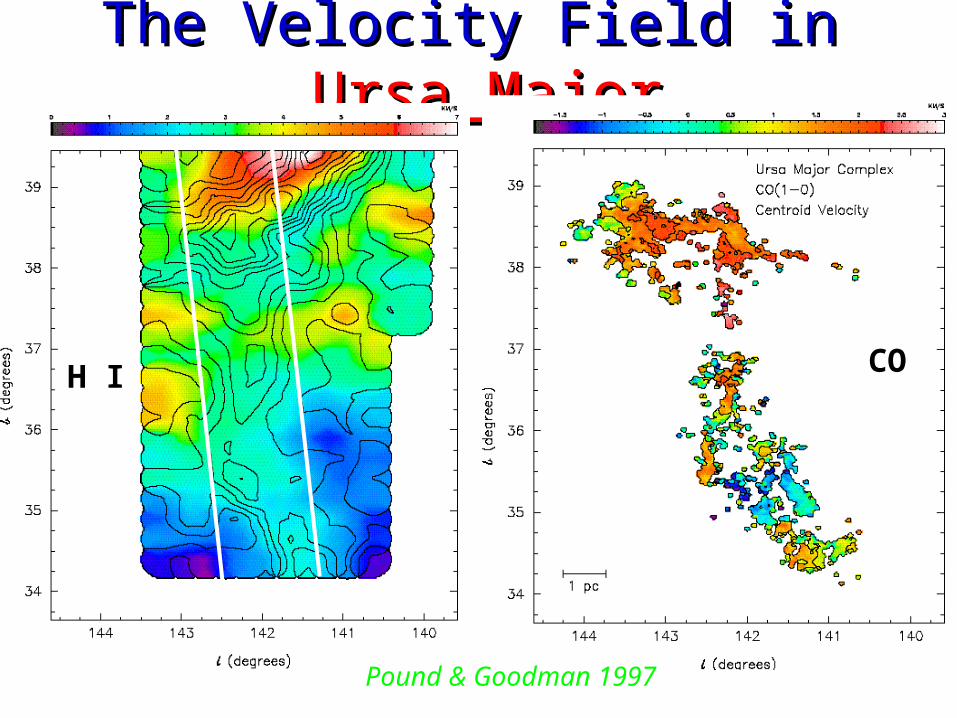
The Velocity Field in The Velocity Field in Ursa MajorUrsa Major
H I CO
Pound & Goodman 1997
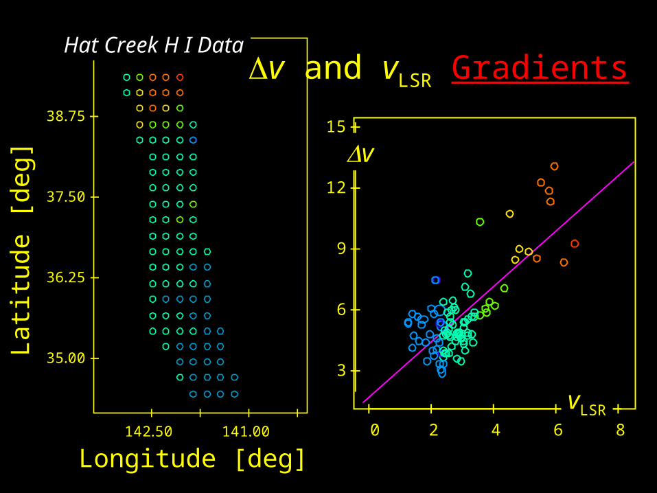
vv and and vvLSRLSR GradientsGradients
35.00
36.25
37.50
38.75
142.50 141.00
3
6
9
12
15
0 2 4 6 8
v
vLSR
Lat
itud
e [d
eg]
Longitude [deg]
Hat Creek H I Data
vz,obs
vz,obs
y
z
Line widthprimarily
tangential
Line widthprimarily
radial
z
-y
vradvtan
Line widthprimarily
radial
Line widthprimarily
tangential
vtanvrad
vtanvrad
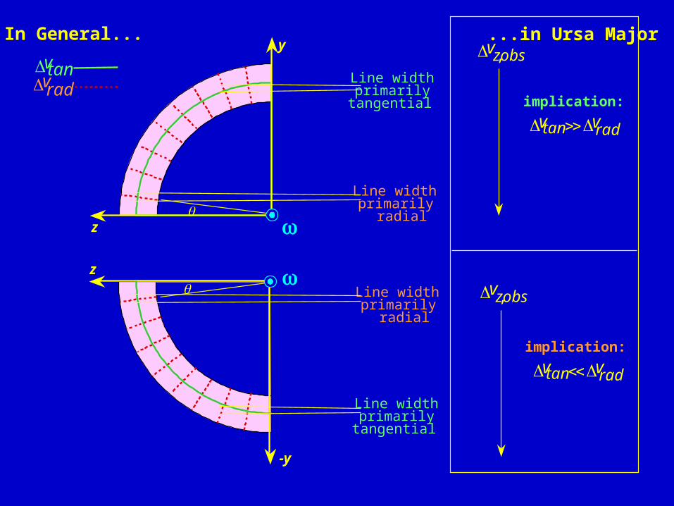
In General... ...in Ursa Major
implication:
implication:
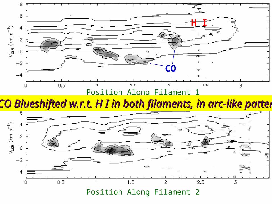
Confirmation: Position Velocity Confirmation: Position Velocity Diagrams for H I and CODiagrams for H I and CO
CO
H I
Position Along Filament 1
Position Along Filament 2
CO Blueshifted w.r.t. H I in both filaments, in arc-like patternCO Blueshifted w.r.t. H I in both filaments, in arc-like pattern
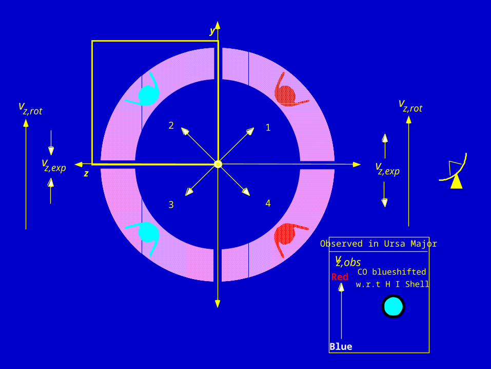
vz,obsRed
Blue
Observed in Ursa Major
CO blueshifted
w.r.t H I Shell
y
2 1
43
vz,rot
vz,exp
vz,rot
vz,expz
Implications of Ursa Major StudyImplications of Ursa Major Study
• Many HLC’s may be related to “supershell” structures; some shells harder to identify than NCP Loop.
• (Commonly observed) velocity offsets between atomic and molecular gas may be due to impacts, followed by conservation of momentum. Use this as a clue in other cases.
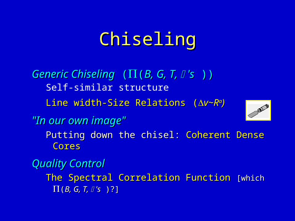
ChiselingChiseling
Generic ChiselingGeneric Chiseling ( (((B, G, T, B, G, T, 's 's )) ))Self-similar structure
Line width-Size RelationsLine width-Size Relations ((v~Rv~Raa))
"In our own image""In our own image"Putting down the chisel:Putting down the chisel: Coherent Dense Cores Coherent Dense Cores
Quality ControlQuality ControlThe Spectral Correlation Function The Spectral Correlation Function [which [which ((B, G, T, B, G, T, 's 's )?] )?]
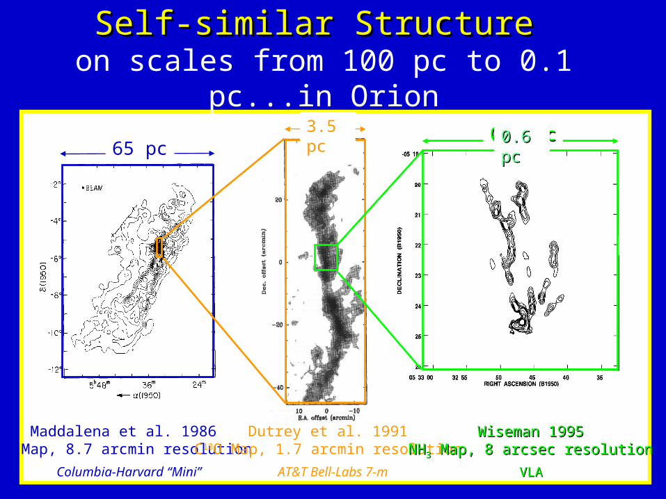
Self-similar StructureSelf-similar Structure on scales from 100 pc to 0.1 pc...in Orion
65 pc
Maddalena et al. 1986CO Map, 8.7 arcmin resolution
Columbia-Harvard “Mini”
Dutrey et al. 1991C18O Map, 1.7 arcmin resolution
AT&T Bell-Labs 7-m
3.5 pc0.6 pc0.6 pc
Wiseman 1995Wiseman 1995NHNH33 Map, 8 arcsec resolution Map, 8 arcsec resolution
VLAVLA
3.5 pc0.6 pc0.6 pc
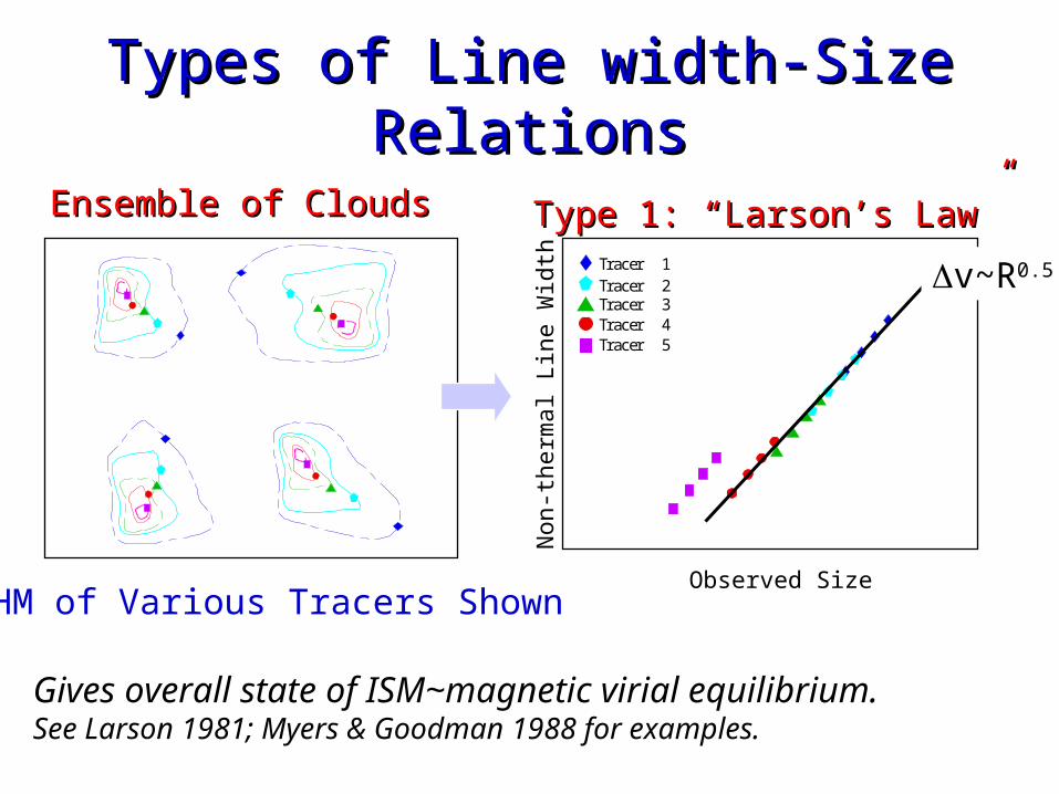
Types of Line width-Size RelationsTypes of Line width-Size Relations
Tracer 5
Tracer 1Tracer 2Tracer 3Tracer 4
Ensemble of CloudsEnsemble of Clouds
FWHM of Various Tracers ShownObserved Size
Non
-th
erm
al
Lin
e W
idth
Type 1: “Larson’s Law”Type 1: “Larson’s Law”
Gives overall state of ISM~magnetic virial equilibrium.See Larson 1981; Myers & Goodman 1988 for examples.
v~R0.5
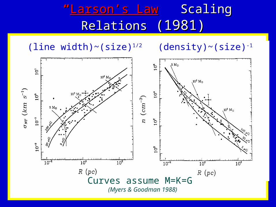
““Larson’s LawLarson’s Law” ” Scaling RelationsScaling Relations (1981)(1981)
(line width)~(size)1/2 (density)~(size)-1
Curves assume M=K=G (Myers & Goodman 1988)
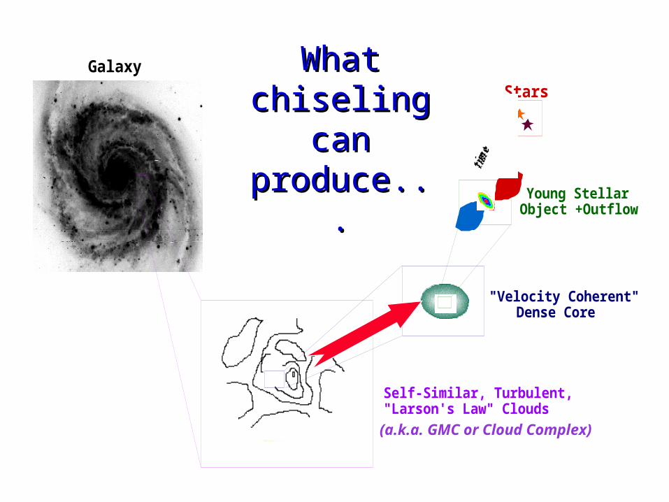
Galaxy
"Velocity Coherent" Dense Core
Young Stellar Object +Outflow
Stars
time
Self-Similar, Turbulent,"Larson's Law" Clouds
What What chiseling can chiseling can
produce...produce...
(a.k.a. GMC or Cloud Complex)
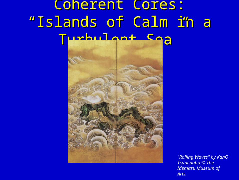
Coherent Cores: “Islands of Calm Coherent Cores: “Islands of Calm in a Turbulent Sea”in a Turbulent Sea”
"Rolling Waves" by KanO Tsunenobu © The Idemitsu Museum of Arts.
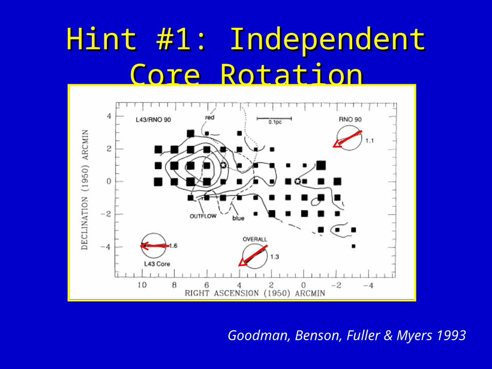
Hint #1: Independent Core RotationHint #1: Independent Core Rotation
Goodman, Benson, Fuller & Myers 1993
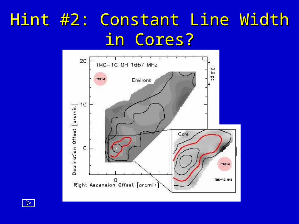
Hint #2: Constant Line Width in Cores?Hint #2: Constant Line Width in Cores?
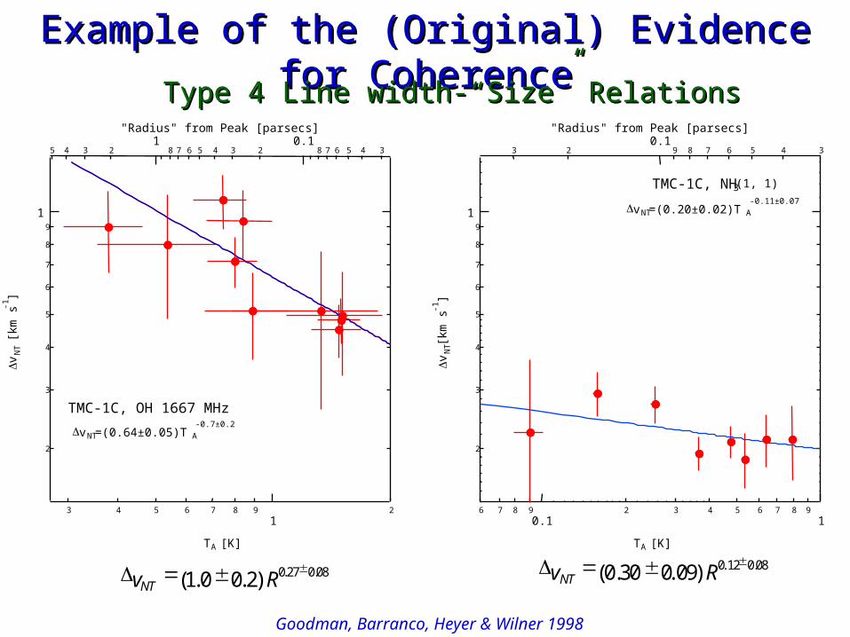
Example of the (Original) Evidence for CoherenceExample of the (Original) Evidence for Coherence
2
3
4
5
6
7
8
9
1
vN
T[km
s-1
]
6 7 8 90.1
2 3 4 5 6 7 8 91
TA [K]
34567890.1
23
"Radius" from Peak [parsecs]
TMC-1C, NH3 (1, 1)
vNT=(0.20±0.02)T A-0.11±0.07
2
3
4
5
6
7
8
9
1
vN
T [k
m s
-1]
3 4 5 6 7 8 91
2
TA [K]
3456780.1
23456781
2345
"Radius" from Peak [parsecs]
vNT=(0.64±0.05)T A-0.7±0.2
TMC-1C, OH 1667 MHz
vNT(1.00.2)R0.270.08 vNT
(0.300.09)R0.120.08
Type 4 Line width-“Size” RelationsType 4 Line width-“Size” Relations
Goodman, Barranco, Heyer & Wilner 1998
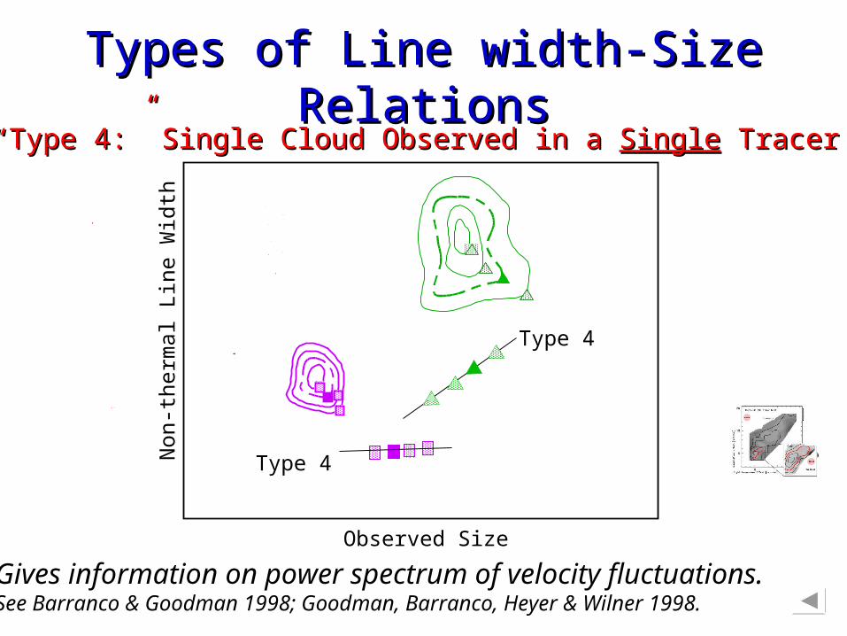
Types of Line width-Size RelationsTypes of Line width-Size Relations““Type 4:” Single Cloud Observed in a Type 4:” Single Cloud Observed in a SingleSingle Tracer Tracer
Gives information on power spectrum of velocity fluctuations.See Barranco & Goodman 1998; Goodman, Barranco, Heyer & Wilner 1998.
Observed Size
Type 4
Type 4
Non
-th
erm
al
Lin
e W
idth
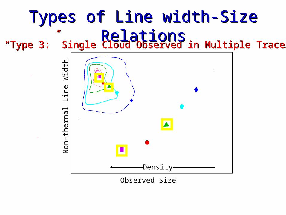
Types of Line width-Size RelationsTypes of Line width-Size Relations
Observed Size
““Type 3:” Single Cloud Observed in Multiple TracersType 3:” Single Cloud Observed in Multiple Tracers
Non
-th
erm
al
Lin
e W
idth
Density
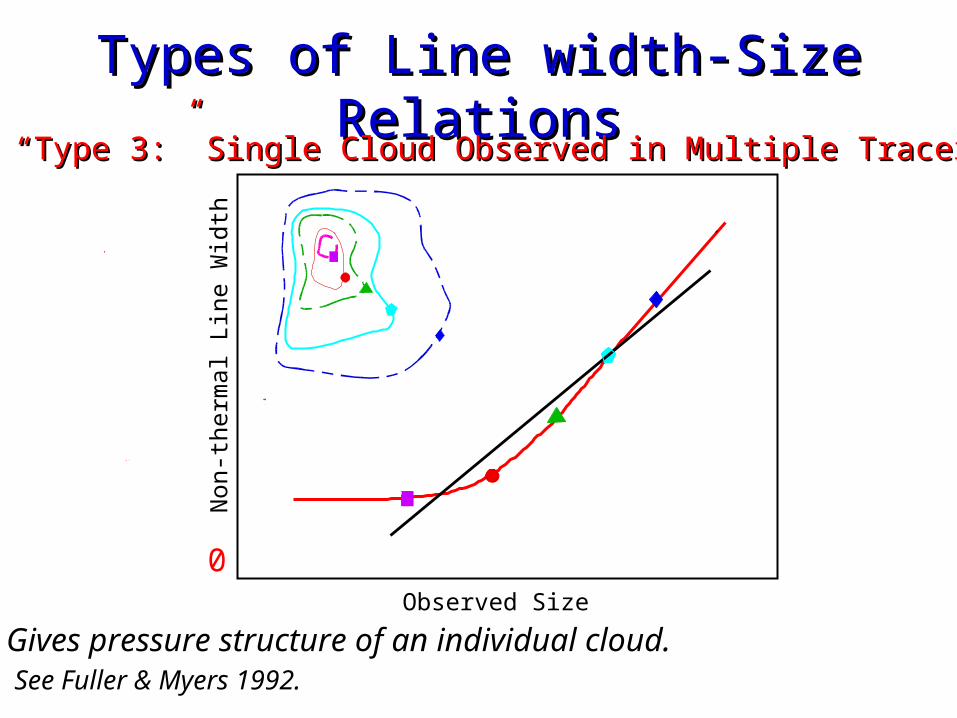
Types of Line width-Size RelationsTypes of Line width-Size Relations
Observed Size
““Type 3:” Single Cloud Observed in Multiple TracersType 3:” Single Cloud Observed in Multiple Tracers
Non
-th
erm
al
Lin
e W
idth
Gives pressure structure of an individual cloud. See Fuller & Myers 1992.
0
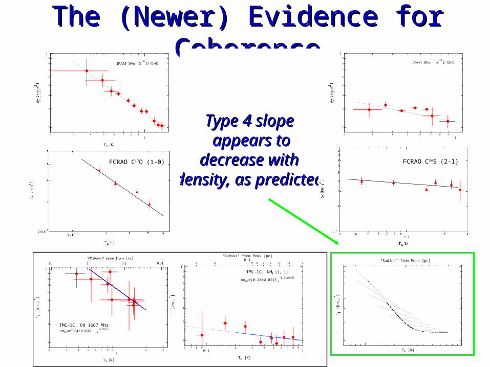
The (Newer) Evidence for CoherenceThe (Newer) Evidence for Coherence
2
3
4
5
6
7
8
9
1
0.1 2 10x-1 3 4
TA [ ]K
FCRAO C34
(2-1)S
2
3
4
5
6
7
8
9
1
2 3 4 5 6 7 8 91
TA [ ]K
30- IRAM m C34
(2-1)S
2
3
4
5
6
7
8
9
1
2 3 4 5 6 7 8 91
TA [ ]K
30- IRAM m C17
(1-0)O
2
3
4
5
6
7
8
9
1
4 10x0 5 6
TA [ ]K
30- IRAM m C18
(2-1)O
2
3
4
5
6
7
8
9
1
2 10x-1 3 4 5 6
TA [ ]K
FCRAO C17
(1-0)O
2
3
4
5
6
7
8
9
1
2 3 4 5 6 7 8 91
2 3
TA [ ]K
0.010.1110" " [ ]Radius from Peak pc
vNT=(0.64±0.05)T A-0.7±0.2
TMC-1C, OH 1667 MHz
2
3
4
5
6
7
8
9
1
6 7 8 90.1
2 3 4 5 6 7 8 91
TA [K]
34567890.1
23
"Radius" from Peak [pc]
TMC-1C, NH3 (1, 1)
ΔvNT=(0.20±0.02)T A-0.11±0.07
2
3
4
5
6
7
8
9
1
6 7 8 90.1
2 3 4 5 6 7 8 91
2
TA [K]
FCRAO C18
O (1-0)
"Radius" from Peak [pc]
TA [K]
Type 4 slope Type 4 slope appears toappears to
decrease with decrease with density, as predicted.density, as predicted.
FCRAO C17O (1-0) FCRAO C34S (2-1)
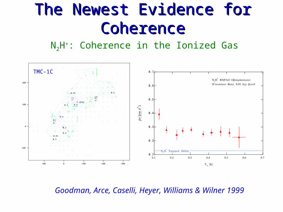
The Newest Evidence for CoherenceThe Newest Evidence for Coherence
0.7
0.6
0.5
0.4
0.3
0.2
0.1
[ v km s
-1 ]
0.70.60.50.40.30.20.1
TA [ ]K
N2H+ Thermal Width
N2H+ FCRAO Observations
( , 0.05 )Gaussian Fits deg bins200
100
0
-100
-300-200-1000100
0.5
0.5
0.5
0.45
0.45
0.4
0.4
0.4
0.35
0.35
0.35
0.3
0.3
N2H+: Coherence in the Ionized Gas
Goodman, Arce, Caselli, Heyer, Williams & Wilner 1999
TMC-1C
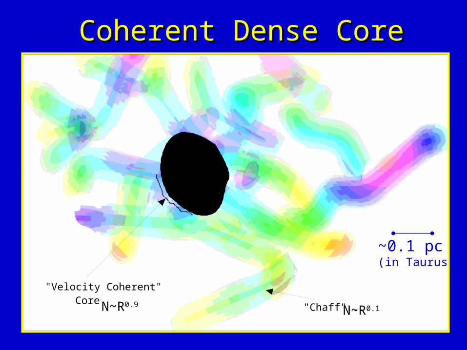
Coherent Dense CoreCoherent Dense Core
"Velocity Coherent"Core
"Chaff"...
~0.1 pc(in Taurus)
N~R0.1N~R0.9
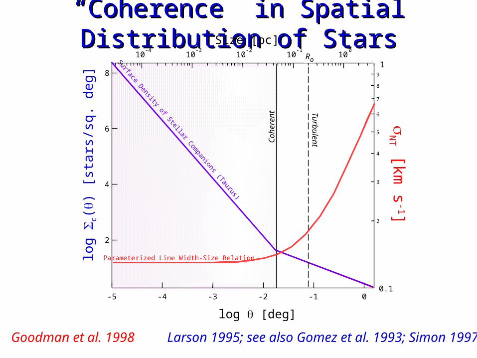
““Coherence” in Spatial Distribution of Coherence” in Spatial Distribution of StarsStars
Surface Density of Stellar Companions (Taurus)
Parameterized Line Width-Size Relation
Coherent T
urbulent
8
6
4
2
log
c()
[st
ars/
sq. d
eg]
-5 -4 -3 -2 -1 0
log [deg]
10-4
10-3
10-2
10-1
100
Size [pc]Ro
0.1
2
3
4
5
6
7
8
9
1
N
T [km s
-1]
Larson 1995; see also Gomez et al. 1993; Simon 1997Goodman et al. 1998
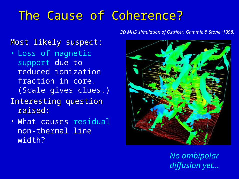
The Cause of Coherence?The Cause of Coherence?
No ambipolardiffusion yet...
3D MHD simulation of Ostriker, Gammie & Stone (1998)
Most likely suspect:Most likely suspect:• Loss of magnetic
support due to reduced ionization fraction in core. (Scale gives clues.)
Interesting question raised:Interesting question raised:• What causes residual
non-thermal line width?
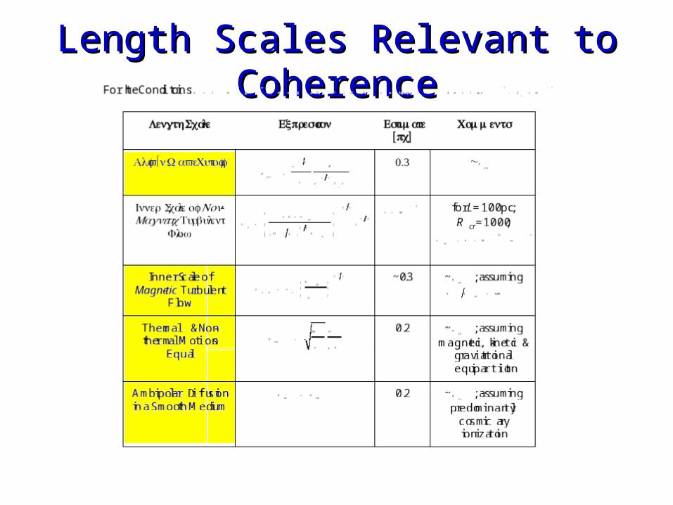
Length Scales Relevant to CoherenceLength Scales Relevant to Coherence
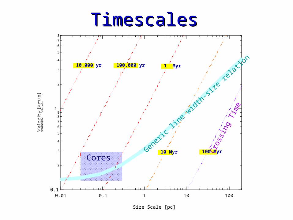
0.1
2
3
4
5
6
789
1
2
3
4
5
6
78
Velocity [km/s]
0.01 0.1 1 10 100
Size Scale [pc]
100 Myr 10 Myr
1 Myr 100,000 yr 10,000 yr
TimescalesTimescales
Cro
ssin
g Ti
me
Gener
ic lin
e wid
th-s
ize re
latio
n
Cores
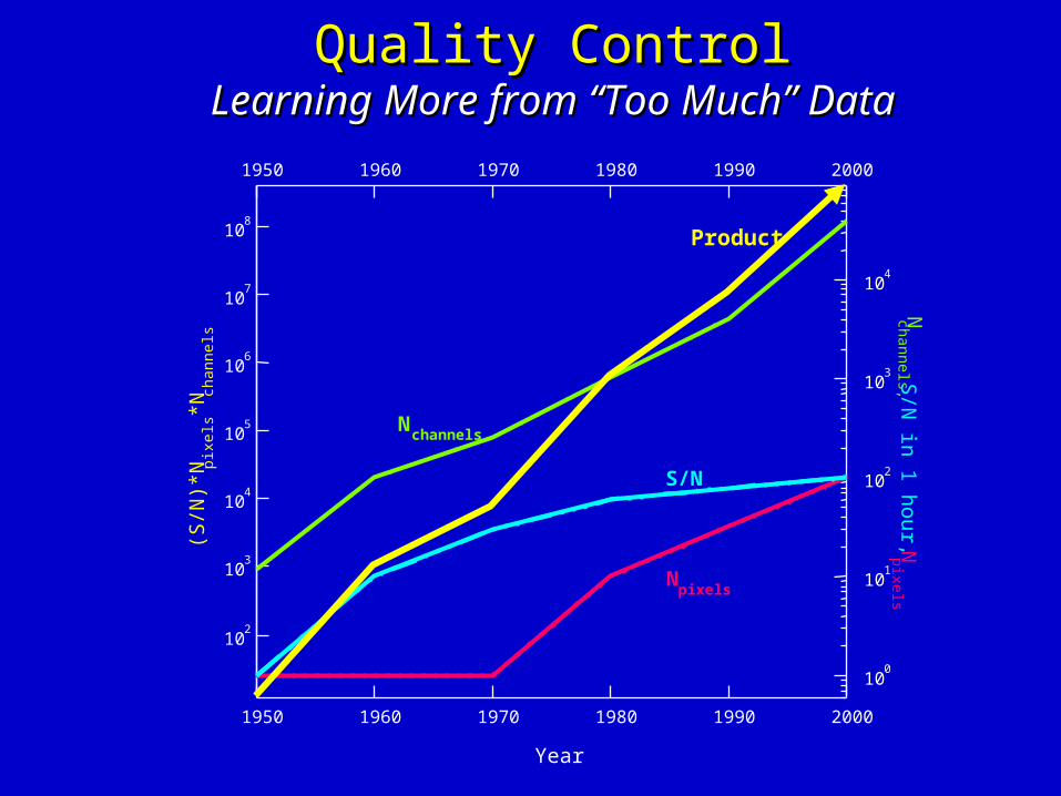
Quality ControlQuality ControlLearning More from “Too Much” DataLearning More from “Too Much” Data
2000
2000
1990
1990
1980
1980
1970
1970
1960
1960
1950
1950
Year
100
101
102
103
104
Nch
an
nels, S
/N in
1 h
our, N
pix
els
102
103
104
105
106
107
108
(S/N
)*N
pix
els
*Nch
an
nels
Npixels
S/N
Product
Nchannels
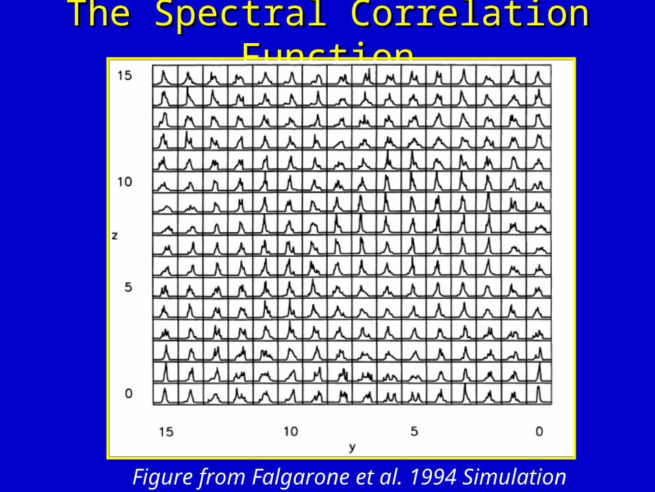
The Spectral Correlation FunctionThe Spectral Correlation Function
Figure from Falgarone et al. 1994 Simulation
Goals of “SCF” ProjectGoals of “SCF” Project• Develop a “sharp tool” for statistical analysis of ISM,
using as much data of a data cube as possible• Compare information from this tool with other tools
(e.g CLUMPFIND, GAUSSCLUMPS, ACF, Wavelets), applied to same cubes
• Use best suite of tools to compare “real” & “simulated” ISM
• Adjust simulations to match, understanding physical inputs
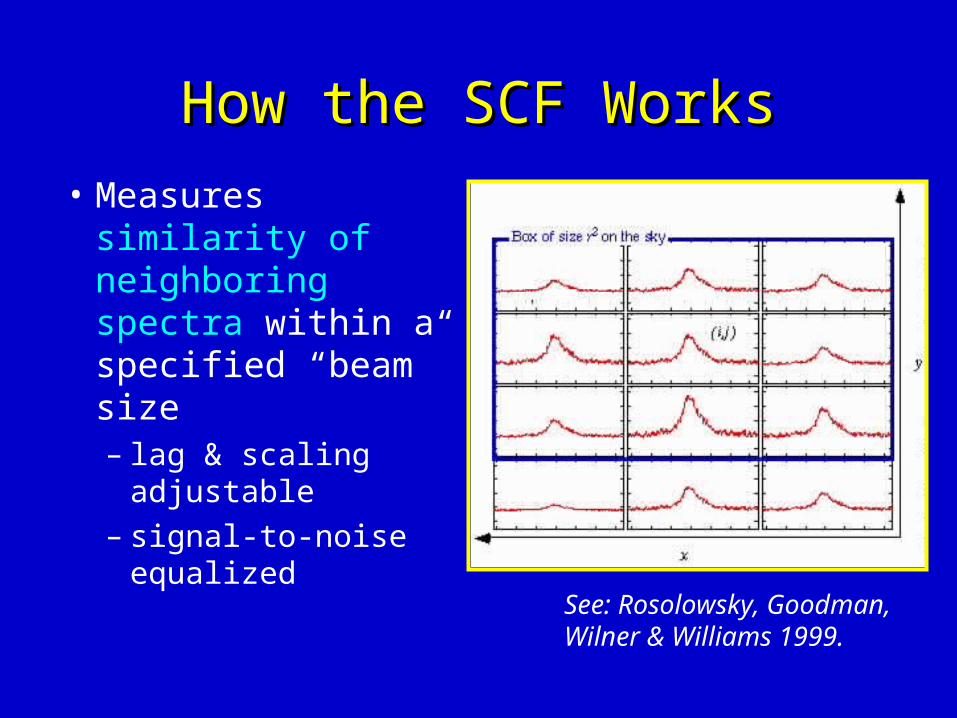
How the SCF WorksHow the SCF Works
• Measures similarity of neighboring spectra within a specified “beam” size– lag & scaling
adjustable– signal-to-noise
equalized See: Rosolowsky, Goodman, Wilner & Williams 1999.
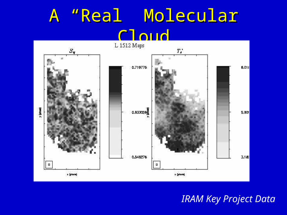
A “Real” Molecular CloudA “Real” Molecular Cloud
IRAM Key Project Data
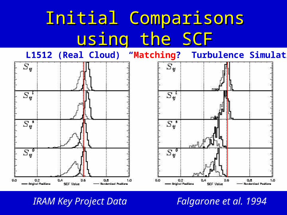
Initial Comparisons using the SCFInitial Comparisons using the SCF
Falgarone et al. 1994
L1512 (Real Cloud) “Matching?” Turbulence Simulation
IRAM Key Project Data
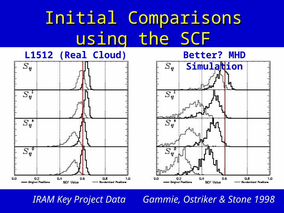
Initial Comparisons using the SCFInitial Comparisons using the SCF
Gammie, Ostriker & Stone 1998
L1512 (Real Cloud)
IRAM Key Project Data
Better? MHD Simulation
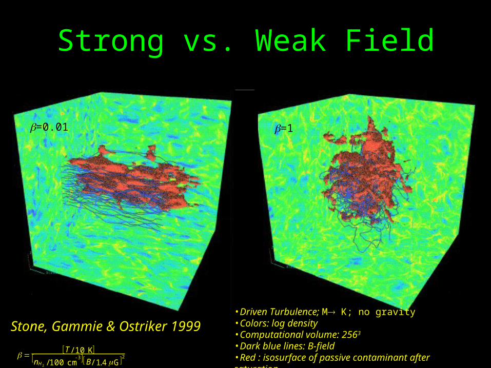
Strong vs. Weak Field
Stone, Gammie & Ostriker 1999•Driven Turbulence; M K; no gravity•Colors: log density•Computational volume: 2563
•Dark blue lines: B-field•Red : isosurface of passive contaminant after saturation
=0.01 =1
T / 10 K
nH 2 / 100 cm-3 B / 1.4 G 2

Goals of “SCF” ProjectGoals of “SCF” Project• Develop a “sharp tool” for statistical analysis of ISM,
using as much data of a data cube as possible• Compare information from this tool with other tools
(e.g CLUMPFIND, GAUSSCLUMPS, ACF, Wavelets), applied to same cubes
• Use best suite of tools to compare “real” & “simulated” ISM
• Adjust simulations to match, understanding physical inputs
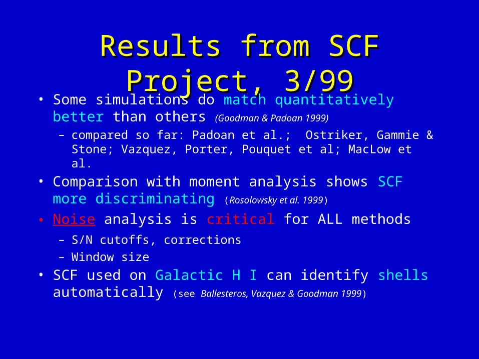
Results from SCF Project, 3/99Results from SCF Project, 3/99• Some simulations do match quantitatively better than
others (Goodman & Padoan 1999)
– compared so far: Padoan et al.; Ostriker, Gammie & Stone; Vazquez, Porter, Pouquet et al; MacLow et al.
• Comparison with moment analysis shows SCF more discriminating (Rosolowsky et al. 1999)
• Noise analysis is critical for ALL methods– S/N cutoffs, corrections
– Window size
• SCF used on Galactic H I can identify shells automatically (see Ballesteros, Vazquez & Goodman 1999)
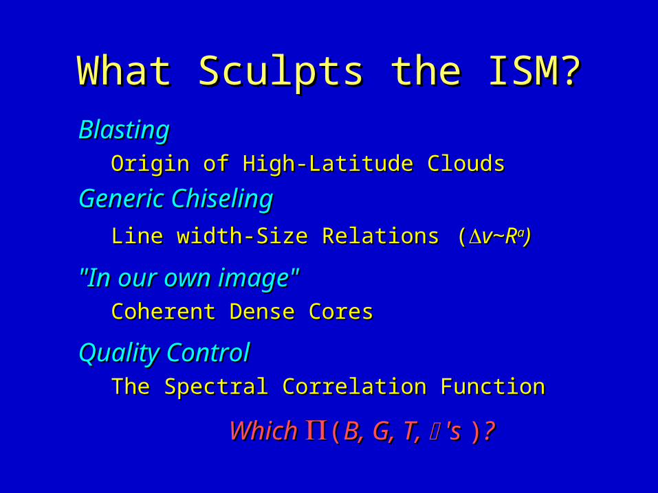
What Sculpts the ISM?What Sculpts the ISM?BlastingBlasting
Origin of High-Latitude CloudsOrigin of High-Latitude Clouds
Generic ChiselingGeneric Chiseling
Line width-Size RelationsLine width-Size Relations ((v~Rv~Raa))
"In our own image""In our own image"Coherent Dense CoresCoherent Dense Cores
Quality ControlQuality ControlThe Spectral Correlation FunctionThe Spectral Correlation Function
Which Which ((B, G, T, B, G, T, 's 's ))??
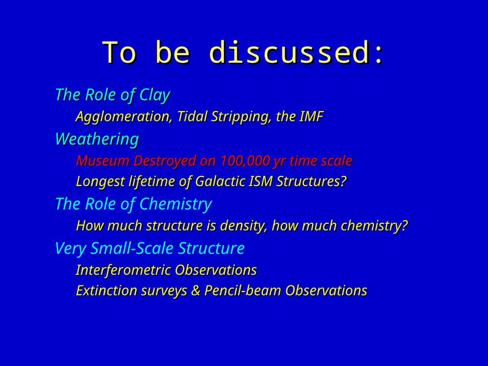
To be discussed:To be discussed:The Role of ClayThe Role of Clay
Agglomeration, Tidal Stripping, the IMFAgglomeration, Tidal Stripping, the IMF
WeatheringWeathering Museum Destroyed on 100,000 yr time scaleMuseum Destroyed on 100,000 yr time scale
Longest lifetime of Galactic ISM Structures?Longest lifetime of Galactic ISM Structures?
The Role of ChemistryHow much structure is density, how much chemistry?How much structure is density, how much chemistry?
Very Small-Scale StructureInterferometric ObservationsInterferometric Observations
Extinction surveys & Pencil-beam ObservationsExtinction surveys & Pencil-beam Observations
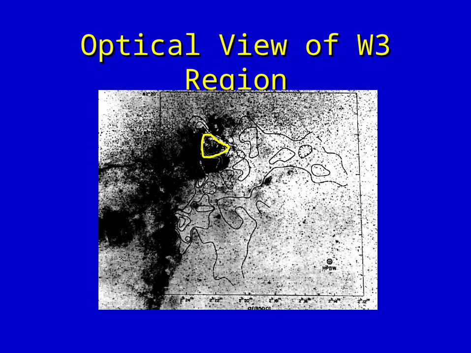
Optical View of W3 RegionOptical View of W3 Region
The Velocity Field in The Velocity Field in Ursa MajorUrsa Major
Pound & Goodman 1997


