Water scarcity and the impact of improved irrigation management: A CGE analysis by Alvaro Calzadilla, Katrin Rehdanz and Richard S.J. Tol
No. 1436 | July 2008
Kiel Institute for the World Economy, Düsternbrooker Weg 120, 24105 Kiel, Germany
Kiel Working Paper No. 1436 | July 2008
Water scarcity and the impact of improved irrigation management: A CGE
analysis
Alvaro Calzadilla, Katrin Rehdanz and Richard S.J. Tol Abstract: We use the new version of the GTAP-W model to analyze the economy-wide impacts of enhanced irrigation efficiency. The new production structure of the model, which introduces a differentiation between rainfed and irrigated crops, allows a better understanding of the use of water resources in agricultural sectors. The results indicate that a water policy directed to improvements in irrigation efficiency in water-stressed regions is not beneficial for all. For water-stressed regions the effects on welfare and demand for water are mostly positive. For non-water scarce regions the results are more mixed and mostly negative. Global water savings are achieved. Not only regions where irrigation efficiency changes are able to save water, but also other regions are pushed to conserve water.
Keywords: Computable General Equilibrium, Irrigation, Water Policy, Water Scarcity, Irrigation efficiency
JEL classification: D58, Q17, Q25 Alvaro Calzadilla Research unit Sustainability and Global Change, Hamburg University and Centre for Marine and Atmospheric Science, Hamburg; International Max Planck Research School on Earth System Modelling, Hamburg E-mail: [email protected]
Richard S.J. Tol Economic and Social Research Institute, Dublin, Ireland; Institute for Environmental Studies, Vrije Universiteit, Amsterdam, The Netherlands; Department of Spatial Economics, Vrije Universiteit, Amsterdam, The Netherlands; Engineering and Public Policy, Carnegie Mellon University, Pittsburgh, PA, USA E-mail: [email protected]
Katrin Rehdanz Christian-Albrechts University of Kiel Department of Economics Olshausenstrasse 40 24118 Kiel, Germany The Kiel Institute for the World Economy, Kiel, Germany E-mail: [email protected]
____________________________________ The responsibility for the contents of the working papers rests with the author, not the Institute. Since working papers are of a preliminary nature, it may be useful to contact the author of a particular working paper about results or caveats before referring to, or quoting, a paper. Any comments on working papers should be sent directly to the author. Coverphoto: uni_com on photocase.com
WATER SCARCITY AND THE IMPACT OF IMPROVED IRRIGATION
MANAGEMENT: A CGE ANALYSIS
Alvaro Calzadilla a,b, Katrin Rehdanz a,c,d and Richard S.J. Tol e,f,g,h
July 2008
a Research unit Sustainability and Global Change, Hamburg University and Centre for Marine and Atmospheric Science, Hamburg, Germany
b International Max Planck Research School on Earth System Modelling, Hamburg, Germany c Christian-Albrechts-University of Kiel, Department of Economics, Kiel, Germany d Kiel Institute for the World Economy, Kiel, Germany e Economic and Social Research Institute, Dublin, Ireland f Institute for Environmental Studies, Vrije Universiteit, Amsterdam, The Netherlands g Department of Spatial Economics, Vrije Universiteit, Amsterdam, The Netherlands h Engineering and Public Policy, Carnegie Mellon University, Pittsburgh, PA, USA
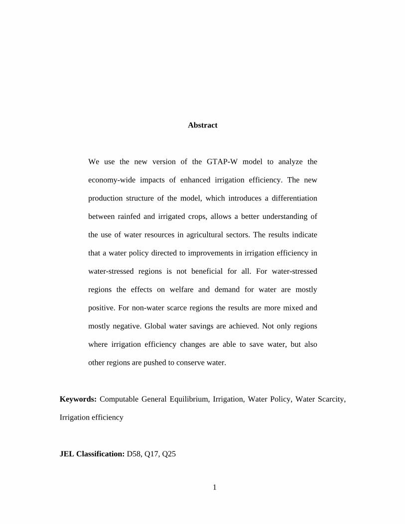
Abstract
We use the new version of the GTAP-W model to analyze the
economy-wide impacts of enhanced irrigation efficiency. The new
production structure of the model, which introduces a differentiation
between rainfed and irrigated crops, allows a better understanding of
the use of water resources in agricultural sectors. The results indicate
that a water policy directed to improvements in irrigation efficiency in
water-stressed regions is not beneficial for all. For water-stressed
regions the effects on welfare and demand for water are mostly
positive. For non-water scarce regions the results are more mixed and
mostly negative. Global water savings are achieved. Not only regions
where irrigation efficiency changes are able to save water, but also
other regions are pushed to conserve water.
Keywords: Computable General Equilibrium, Irrigation, Water Policy, Water Scarcity,
Irrigation efficiency
JEL Classification: D58, Q17, Q25
1
Aristotle wondered why useless diamonds are expensive, while essential drinking water
is free. Any economist since Jevons knows that this is because diamonds are scarce,
while water is abundant – at least, when Aristotle lived. Nowadays, water is scarce and
therefore should command a price. However, both water management and economics
have been slow to adapt to this new reality. This article contributes directly to the latter
and indirectly to the former.
Several factors contribute to water scarcity. Average annual precipitation may be
low, or it may be highly variable. Moreover, population growth and an increasing
consumption of water per capita have resulted in a rapid increase in the demand for
water. This tendency is likely to continue as water consumption for most uses is projected
to increase by at least 50% by 2025 compared to 1995 level (Rosegrant, Cai and Cline
2002). Since the annually renewable fresh water available in a particular location is
typically constant, water scarcity is increasingly constraining food production.
As the supply of water is limited, attempts have been made to economize on the
consumption of water, especially in regions where the supply is critical (Seckler, Molden
and Barker 1998; Dinar and Yaron 1992). Since the agricultural sector accounts for about
70 percent of renewable fresh water use worldwide one way to address the problem is to
reduce the inefficiencies in irrigation. Irrigated agriculture uses about 18 percent of the
total arable land and produces about 33 percent of total agricultural output (Johansson et
al. 2002). However, expanding irrigated areas might not be sufficient to ensure future
food-security and meet the increasing demand for water in populous but water-scarce
regions (Kamara and Sally 2004).
2

Furthermore, in many regions water is free or subsidized (Rosegrant, Cai and
Cline 2002) and for many countries the average irrigation efficiency is low (Seckler,
Molden and Barker 1998). The current level and structure of water charges mostly do not
encourage farmers to use water more efficiently. An increase in water price, for instance
by a tax, would lead to the adoption of improved irrigation technology and water savings
(e.g. Dinar and Yaron 1992; Tsur et al. 2004; Easter and Liu 2005). The water saved
could be used in other sectors, for which the value is much higher. More efficient use
would enhance sustainable irrigation with lower environmental impacts including soil
degradation (erosion, salination, etc.). However, there are many components of water
pricing which make it difficult to determine the marginal value of water (see e.g.
Johansson et al. 2002). Furthermore, in their study for northern China, Yang, Zhang and
Zehnder (2003) point out that pricing alone is not enough to encourage water
conservation. Water rights need to be clearly defined and legally enforceable,
responsibilities for water operators and users identified. Wichelns (2003) discusses the
importance of non-water inputs and farm-level constrains for water use and agricultural
productivity. He investigates policies that modify farm-level input and output prices
directly, international trade policies, policies that revise regulations on land tenure and
sources of investment funds.
An alternative, although limited, strategy to meet the increasing demand for water
is the use of non-conventional water resources including desalination of seawater,
purification of highly brackish groundwater, harvesting of rainwater, as well as the use of
marginal-quality water resources (Ettouney et al. 2002; Zhou and Tol 2005; Qadir et al.
3
2007). Continued progress in desalination technology has lead to considerably lower
costs for water produced. However, costs are still too high for agricultural use. Marginal-
quality water contains one or more impurities at levels that might be harmful to human
and animal health.
Most of the existing literature related to irrigation water use investigates irrigation
management, water productivity and water use efficiency. One strand of literature
compares the performance of irrigation systems and irrigation strategies in general (e.g.
Pereira 1999; Pereira, Oweis and Zairi 2002). Others have a clear regional focus and
concentrate on specific crop types. To provide a few examples from this extensive
literature; Deng et al. (2006) investigate improvements in agricultural water use
efficiency in arid and semiarid areas of China. Bluemling, Yang and Pahl-Wostl (2007)
study wheat-maize cropping pattern in the North China plain. Mailhol et al. (2004)
analyze strategies for durum wheat production in Tunisia. Lilienfeld and Asmild (2007)
estimate excess water use in irrigated agriculture in western Kansas.
As the above examples indicate, water problems related to irrigation management
are typically studied at the farm-level, the river-catchment-level or the country-level.
About 70 percent of all water is used for agriculture, and agricultural products are traded
internationally. A full understanding of water use and the effect of improved irrigation
management is impossible without understanding the international market for food and
related products, such as textiles. We use the new version of the GTAP-W model, based
on GTAP 6, to analyze the economy-wide impacts of enhanced irrigation efficiency. The
new production structure of the model, which introduces a differentiation between rainfed
4
and irrigated crops, allows a better understanding of the use of water resources in
agricultural sectors. Efforts towards improving irrigation management, e.g. through more
efficient irrigation methods, benefit societies by saving large amounts of water. These
would be available for other uses. The aim of our article is to analyze if improvements in
irrigation management would be economically beneficial for the world as a whole as well
as for individual countries and whether and to what extent water savings could be
achieved.
The remainder of the article is organized as follows: the next section briefly
reviews the literature on economic models of water use. Section 3 presents the new
GTAP-W model and the data on water resources and water use. Section 4 lays down the
three simulation scenarios with no constraints on water availability. Section 5 discusses
the results and section 6 concludes.
Economic models of water use
Economic models of water use have generally been applied to look at the direct effects of
water policies, such as water pricing or quantity regulations, on the allocation of water
resources. In order to obtain insights from alternative water policy scenarios on the
allocation of water resources, partial and general equilibrium models have been used.
While partial equilibrium analysis focus on the sector affected by a policy measure
assuming that the rest of the economy is not affected, general equilibrium models
consider other sectors or regions as well to determine the economy-wide effect; partial
equilibrium models tend to have more detail. Most of the studies using either of the two
5
approaches analyze pricing of irrigation water only (for an overview of this literature see
Johannson et al. 2002). Rosegrant, Cai and Cline (2002) use the IMPACT-WATER
model to estimate demand and supply of food and water to 2025. Fraiture et al. (2004)
extend this to include virtual water trade, using cereals as an indicator. Their results
suggest that the role of virtual water trade is modest. While the IMPACT-WATER model
covers a wide range of agricultural products and regions, other sectors are excluded; it is
a partial equilibrium model.
Studies of water use using general equilibrium approaches are generally based on
data for a single country or region assuming no effects for the rest of the world of the
implemented policy. Therefore, none of these studies is able to look at the global impact
of improvements in irrigation management. Decaluwé, Patry and Savard (1999) analyze
the effect of water pricing policies on demand and supply of water in Morocco. Diao and
Roe (2003) use an intertemporal computable general equilibrium (CGE) model for
Morocco focusing on water and trade policies. Seung et al. (2000) use a dynamic CGE
model to estimate the welfare gains of reallocating water from agriculture to recreational
use for the Stillwater National Wildlife Refuge in Nevada. Letsoalo et al. (2007) and van
Heerden, Blignaut and Horridge (forthcoming) study the effects of water charges on
water use, economic growth, and the real income of rich and poor households in South
Africa. For the Arkansas River Basin, Goodman (2000) shows that temporary water
transfers are less costly than building new dams. Strzepek et al. (forthcoming) estimate
the economic benefits of the High Aswan Dam. Gómez, Tirado and Rey-Maquieira
(2004) analyze the welfare gains by improved allocation of water rights for the Balearic
6

Islands. Feng et al. (2007) use a two-region recursive dynamic general equilibrium
approach based on the GREEN model (Lee, Oliveira-Martins and van der Mensbrugghe
1994) to assess the economic implications of the increased capacity of water supply
through the Chinese South-to-North Water Transfer (SNWT) project. All of these CGE
studies have a limited geographical scope.
Berrittella et al. (2007) are an exception. They use a global CGE model including
water resources (GTAP-W, version 1) to analyze the economic impact of restricted water
supply for water-short regions. They contrast a market solution, where water owners can
capitalize their water rent, to a non-market solution, where supply restrictions imply
productivity losses. They show that water supply constraints could actually improve
allocative efficiency, as agricultural markets are heavily distorted. The welfare gain from
curbing inefficient production may more than offset the welfare losses due to the resource
constraint. Berrittella et al. (forthcoming, a) use the same model to investigate the
economic implications of water pricing policies. They find that water taxes reduce water
use, and lead to shifts in production, consumption and international trade patterns.
Countries that do not levy water taxes are nonetheless affected by other countries’ taxes.
Like Feng et al. (2007), Berrittella, Rehdanz and Tol (2006) analyze the economic effects
of the Chinese SNWT project. Their analysis offers less regional detail but focuses in
particular on the international implications of the project. Berrittella et al. (forthcoming,
b) extend the previous papers by looking at the impact of trade liberalization on water
use.
7

In this article we use the new version of the GTAP-W model to analyze the
economy-wide impacts of enhanced irrigation management through higher levels of
irrigation efficiency. The crucial distinction between version 2 of GTAP-W, used here,
and version 1, used by Berrittella et al., is that version 2 distinguishes rainfed and
irrigated agriculture while version 1 did not make this distinction.
The new GTAP-W model
In order to assess the systemic general equilibrium effects of improved irrigation
management, we use a multi-region world CGE model, called GTAP-W. The model is a
further refinement of the GTAP model1 (Hertel, 1997), and is based on the version
modified by Burniaux and Truong2 (2002) as well as on the previous GTAP-W model
introduced by Berrittella et al. (2007).
The new GTAP-W model is based on the GTAP version 6 database, which
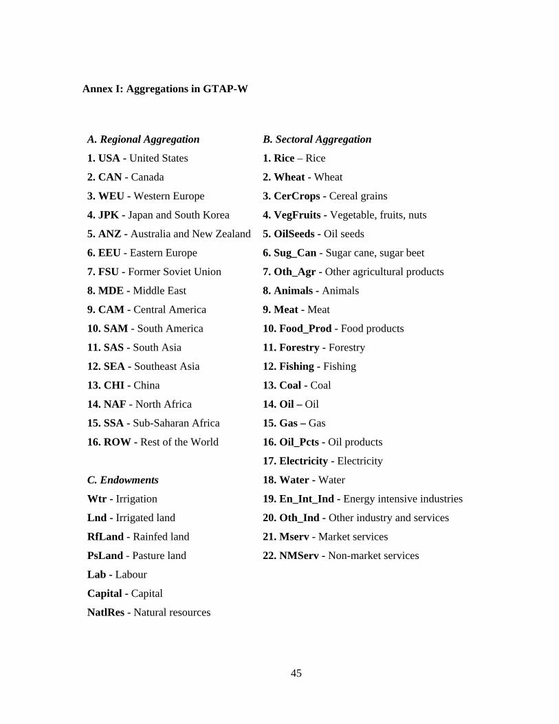
represents the global economy in 2001. The model has 16 regions and 22 sectors, 7 of
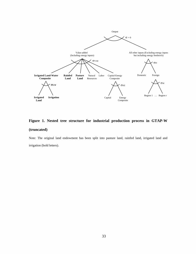
which are in agriculture.3 However, the most significant change and principal
characteristic of version 2 of the GTAP-W model is the new production structure, in
which the original land endowment in the value-added nest has been split into pasture
land and land for rainfed and for irrigated agriculture. Pasture land is basically the land
used in the production of animals and animal products. The last two types of land differ
as rainfall is free but irrigation development is costly. As a result, land equipped for
irrigation is generally more valuable as yields per hectare are higher. To account for this
difference, we split irrigated agriculture further into the value for land and the value for
8
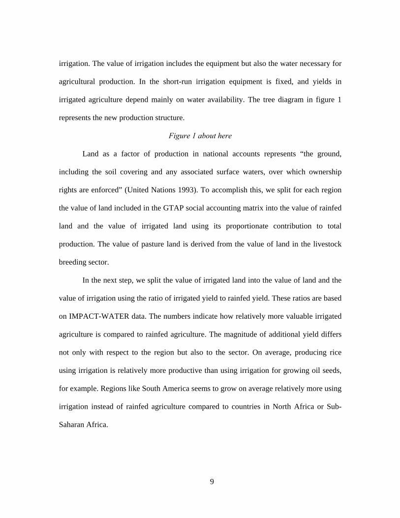
irrigation. The value of irrigation includes the equipment but also the water necessary for
agricultural production. In the short-run irrigation equipment is fixed, and yields in
irrigated agriculture depend mainly on water availability. The tree diagram in figure 1
represents the new production structure.
Figure 1 about here
Land as a factor of production in national accounts represents “the ground,
including the soil covering and any associated surface waters, over which ownership
rights are enforced” (United Nations 1993). To accomplish this, we split for each region
the value of land included in the GTAP social accounting matrix into the value of rainfed
land and the value of irrigated land using its proportionate contribution to total
production. The value of pasture land is derived from the value of land in the livestock
breeding sector.
In the next step, we split the value of irrigated land into the value of land and the
value of irrigation using the ratio of irrigated yield to rainfed yield. These ratios are based
on IMPACT-WATER data. The numbers indicate how relatively more valuable irrigated
agriculture is compared to rainfed agriculture. The magnitude of additional yield differs
not only with respect to the region but also to the sector. On average, producing rice
using irrigation is relatively more productive than using irrigation for growing oil seeds,
for example. Regions like South America seems to grow on average relatively more using
irrigation instead of rainfed agriculture compared to countries in North Africa or Sub-
Saharan Africa.
9
The procedure we described above to introduce the four new endowments
(pasture land, rainfed land, irrigated land and irrigation) allows us to avoid problems
related to model calibration. In fact, since the original database is only split and not
altered, the original regions’ social accounting matrices are balanced and can be used by
the GTAP-W model to assign values to the share parameters of the mathematical
equations. For detailed information about the social accounting matrix representation of
the GTAP database see McDonald, Robinson and Thierfelder (2005).
As in all CGE models, the GTAP-W model makes use of the Walrasian perfect
competition paradigm to simulate adjustment processes. Industries are modelled through
a representative firm, which maximizes profits in perfectly competitive markets. The
production functions are specified via a series of nested constant elasticity of substitution
functions (CES) (figure 1). Domestic and foreign inputs are not perfect substitutes,
according to the so-called ‘‘Armington assumption’’, which accounts for product
heterogeneity.
A representative consumer in each region receives income, defined as the service
value of national primary factors (natural resources, pasture land, rainfed land, irrigated
land, irrigation, labour and capital). Capital and labour are perfectly mobile domestically,
but immobile internationally. Pasture land, rainfed land, irrigated land, irrigation and
natural resources are imperfectly mobile. The national income is allocated between
aggregate household consumption, public consumption and savings. The expenditure
shares are generally fixed, which amounts to saying that the top level utility function has
a Cobb–Douglas specification. Private consumption is split in a series of alternative
10

composite Armington aggregates. The functional specification used at this level is the
constant difference in elasticities (CDE) form: a non-homothetic function, which is used
to account for possible differences in income elasticities for the various consumption
goods. A money metric measure of economic welfare, the equivalent variation, can be
computed from the model output.
In the original GTAP-E model, land is combined with natural resources, labour
and the capital-energy composite in a value-added nest. In our modelling framework, we
incorporate the possibility of substitution between land and irrigation in irrigated
agricultural production by using a nested constant elasticity of substitution function
(figure 1). The procedure how the elasticity of factor substitution between land and
irrigation (σLW) was obtained is explained in more detail in Annex II. Next, the irrigated
land-water composite is combined with pasture land, rainfed land, natural resources,
labour and the capital-energy composite in a value-added nest through a CES structure.
In the benchmark equilibrium, water used for irrigation is supposed to be identical
to the volume of water used for irrigated agriculture in the IMPACT-WATER model. An
initial sector and region specific shadow price for irrigation water can be obtained by
combining the SAM information about payments to factors and the volume of water used
in irrigation from IMPACT-WATER. In this article enhanced irrigation management
including more efficient irrigation water use is introduce in the model through higher
levels of productivity in irrigated production.
11
Design of simulation scenarios
Performance and productivity of irrigated agriculture is commonly measured by the term
irrigation efficiency. For a detailed description and evolution of the irrigation efficiency
terminology see Burt et al. (1997) and Jesen (2007) respectively. In a finite space and
time, FAO (2001) defines irrigation efficiency as the percentage of the irrigation water
consumed by crops to the water diverted from the source of supply. It distinguishes
between conveyance efficiency, which represents the efficiency of water transport in
canals, and the field application efficiency, which represents the efficiency of water
application in the field.
In this article, the term irrigation efficiency indicates the ratio between the volume
of irrigation water beneficially used by the crop to the volume of irrigation water applied
to the crop. In this sense, no distinction is made between conveyance and field
application efficiency. Therefore any improvement in irrigation efficiency refers to an
improvement in the overall irrigation efficiency.
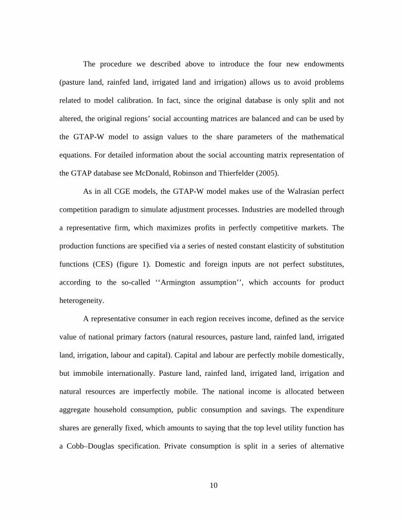
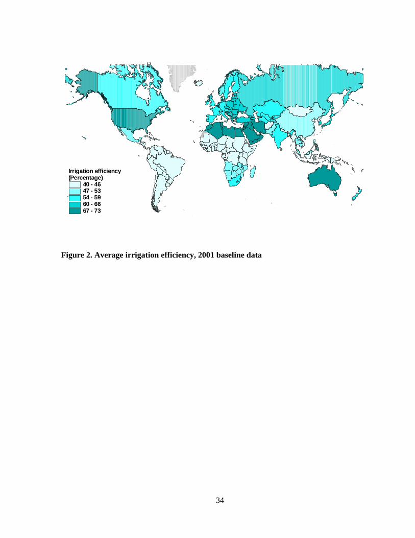
Figure 2 shows a global map of average irrigation efficiency by country. It is
based on the volume of beneficial and non-beneficial irrigation water use provided by the
IMPACT-WATER baseline dataset. The reported irrigation efficiency clearly indicates
that irrigation management in most developing regions is performing poorly, the only
exception is water-scarce North Africa, where levels are comparable to those of
developed regions. Irrigation efficiency in Canada and Western Europe is low. However,
in those two regions irrigated production is not important relative to total production
levels.
12

Figure 2 about here
Certainly, there are differences in performance within regions. Rosegrant, Cai and
Cline (2002) point out that irrigation efficiency ranges between 25 to 40 percent in the
Philippines, Thailand, India, Pakistan and Mexico; between 40 to 45 percent in Malaysia
and Morocco; and between 50 to 60 percent in Taiwan, Israel and Japan. In our analysis,
based on regional averages, these individual effects are averaged out but marked
differences between the regions still exist.
We evaluate the effects on global production and income of enhanced irrigation
efficiency through three different scenarios. The scenarios are designed so as to show a
gradual convergence to higher levels of irrigation efficiency. The first two scenarios
assume that an improvement in irrigation efficiency is more likely in water-scarce
regions. In the first scenario irrigation efficiency in water-stressed developing regions
improves. We consider a region as water-stressed region if at least for one country within
the region water availability is lower than 1,500 cubic meters per person per year.4 These
regions include South Asia (SAS), Southeast Asia (SEA), North Africa (NAF), the
Middle East (MDE), Sub-Saharan Africa (SSA) as well as the Rest of the World (ROW).
The second scenario improves irrigation efficiency in all water-scarce regions
independent of the level of economic development. In addition to the previous scenario
Western Europe (WEU), Eastern Europe (EEU) as well as Japan and South Korea (JPK)
are added to the list of water-short regions. For the first two scenarios, irrigation
efficiency is improved for all irrigated crops in each region to a level of 73 percent.
Comparing with figure 2 above, this is the weighted average level of Australia and New
13
Zealand (ANZ). In the third scenario, we improve irrigation efficiency in all 16 regions
up to 73 percent.
Results
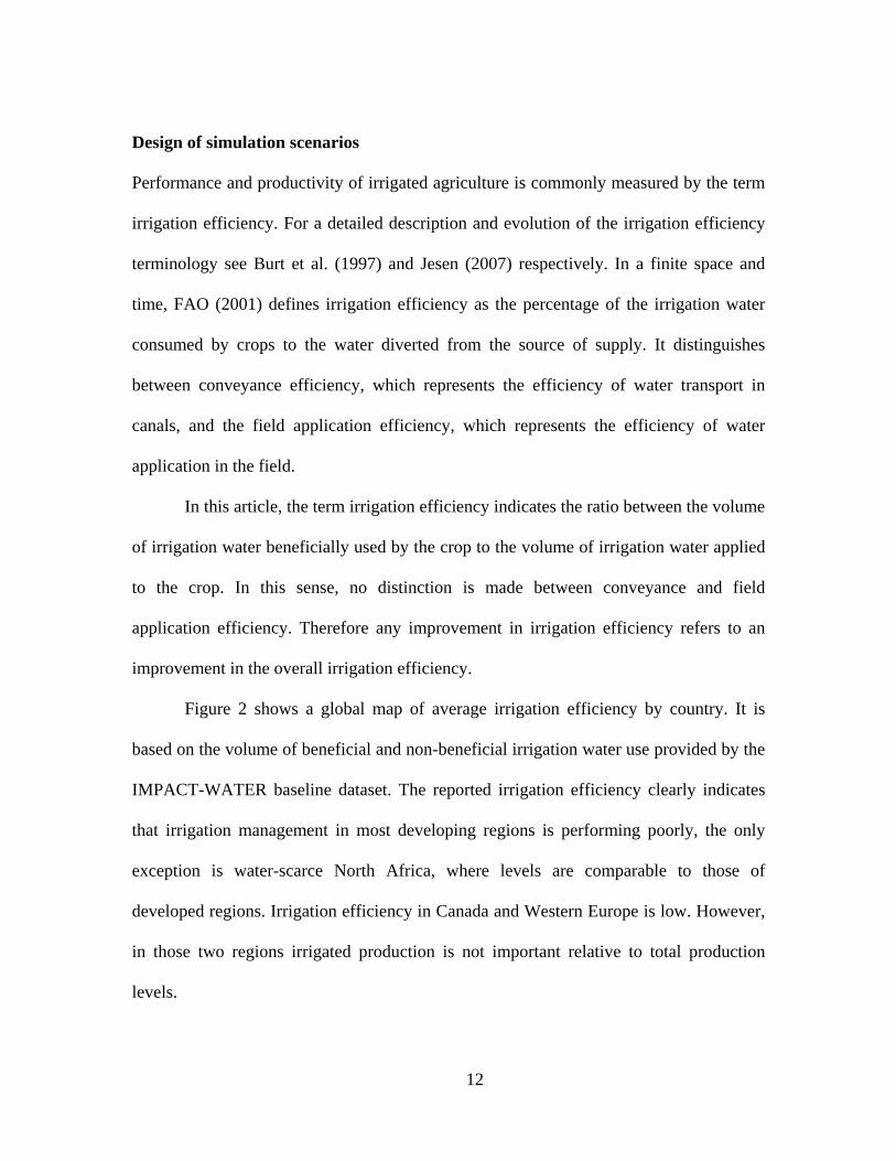
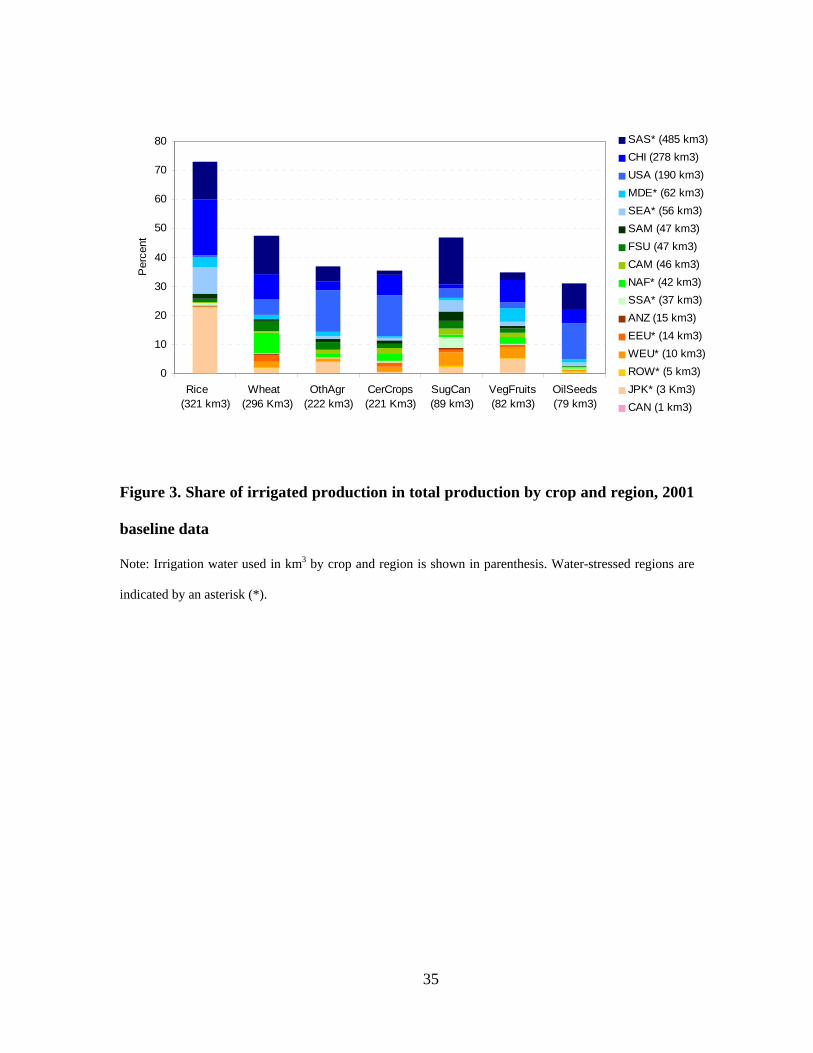
Figure 3 shows irrigated production as share of total agricultural production in the
GTAP-W baseline data. Irrigated rice production accounts for 73 percent of the total rice
production; the major producers are Japan and South Korea, China, South Asia and
Southeast Asia. Around 47 percent of wheat and sugar cane is produced using irrigation.
However, the volume of irrigation water used in sugar cane production is less than one-
third of what is used in wheat production. In irrigated agriculture major producers of
wheat are South Asia, China, North Africa and the USA and for sugar cane South Asia
and Western Europe. The share of irrigated production in total production of the other
four crops in GTAP-W (cereal grains, oil seeds, vegetables and fruits as well as other
agricultural products) varies from 31 to 37 percent. Major producers of cereal grains are
the USA and China; for oil seeds are the USA, South Asia and China; for vegetables and
fruits are China, the Middle East and Japan and South Korea; and for other agricultural
products are the USA and South Asia.
Figure 3 about here
The irrigated production of rice and wheat consumes half of the irrigation water
used globally, and together with cereal grains and other agricultural products the
irrigation water consumption rises to 80 percent. There are three major irrigation water
14
users (South Asia, China and USA). These regions use over 70 percent of the global
irrigation water used, just South Asia uses more than one-third.
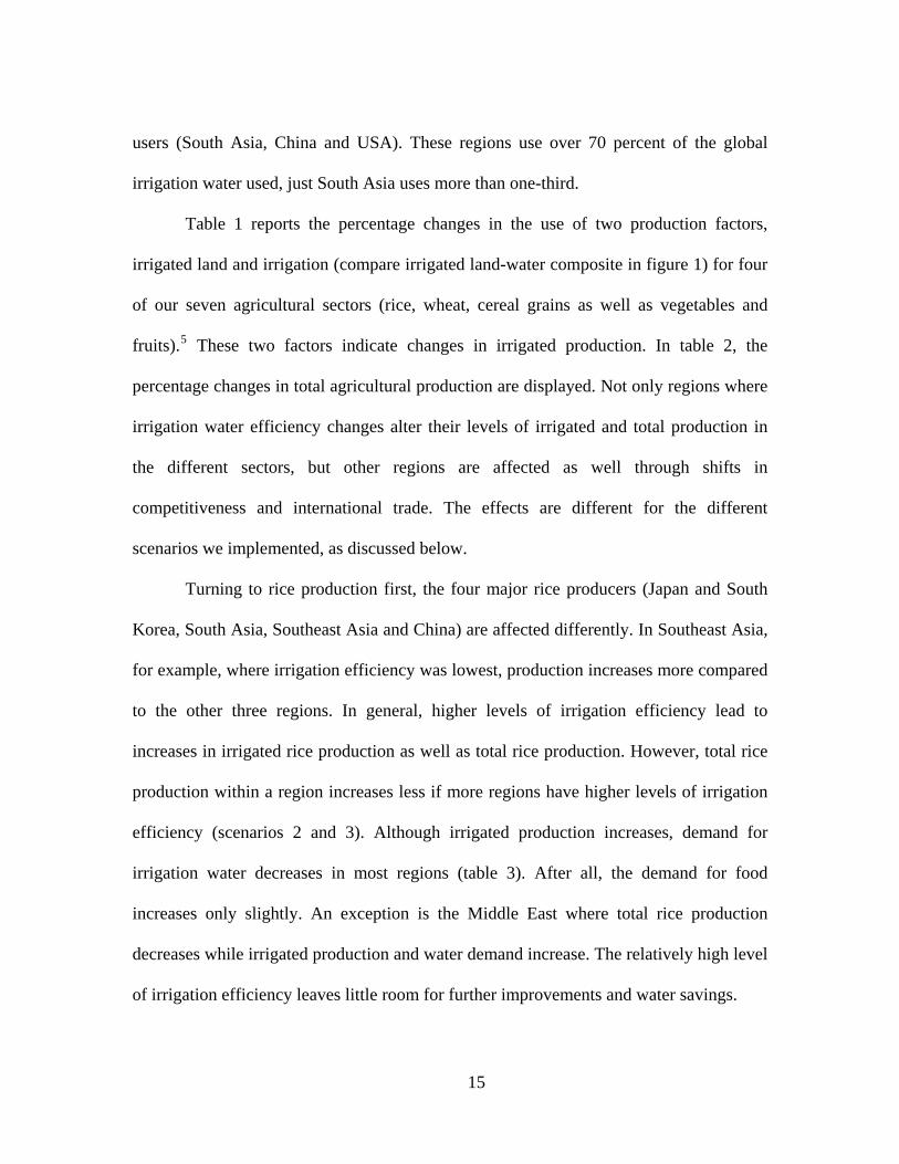
Table 1 reports the percentage changes in the use of two production factors,
irrigated land and irrigation (compare irrigated land-water composite in figure 1) for four
of our seven agricultural sectors (rice, wheat, cereal grains as well as vegetables and
fruits).5 These two factors indicate changes in irrigated production. In table 2, the
percentage changes in total agricultural production are displayed. Not only regions where
irrigation water efficiency changes alter their levels of irrigated and total production in
the different sectors, but other regions are affected as well through shifts in
competitiveness and international trade. The effects are different for the different
scenarios we implemented, as discussed below.
Turning to rice production first, the four major rice producers (Japan and South
Korea, South Asia, Southeast Asia and China) are affected differently. In Southeast Asia,
for example, where irrigation efficiency was lowest, production increases more compared
to the other three regions. In general, higher levels of irrigation efficiency lead to
increases in irrigated rice production as well as total rice production. However, total rice
production within a region increases less if more regions have higher levels of irrigation
efficiency (scenarios 2 and 3). Although irrigated production increases, demand for
irrigation water decreases in most regions (table 3). After all, the demand for food
increases only slightly. An exception is the Middle East where total rice production
decreases while irrigated production and water demand increase. The relatively high level
of irrigation efficiency leaves little room for further improvements and water savings.
15
Tables 1 to 3 about here
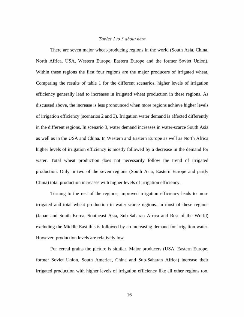
There are seven major wheat-producing regions in the world (South Asia, China,
North Africa, USA, Western Europe, Eastern Europe and the former Soviet Union).
Within these regions the first four regions are the major producers of irrigated wheat.
Comparing the results of table 1 for the different scenarios, higher levels of irrigation
efficiency generally lead to increases in irrigated wheat production in these regions. As
discussed above, the increase is less pronounced when more regions achieve higher levels
of irrigation efficiency (scenarios 2 and 3). Irrigation water demand is affected differently
in the different regions. In scenario 3, water demand increases in water-scarce South Asia
as well as in the USA and China. In Western and Eastern Europe as well as North Africa
higher levels of irrigation efficiency is mostly followed by a decrease in the demand for
water. Total wheat production does not necessarily follow the trend of irrigated
production. Only in two of the seven regions (South Asia, Eastern Europe and partly
China) total production increases with higher levels of irrigation efficiency.
Turning to the rest of the regions, improved irrigation efficiency leads to more
irrigated and total wheat production in water-scarce regions. In most of these regions
(Japan and South Korea, Southeast Asia, Sub-Saharan Africa and Rest of the World)
excluding the Middle East this is followed by an increasing demand for irrigation water.
However, production levels are relatively low.
For cereal grains the picture is similar. Major producers (USA, Eastern Europe,
former Soviet Union, South America, China and Sub-Saharan Africa) increase their
irrigated production with higher levels of irrigation efficiency like all other regions too.
16
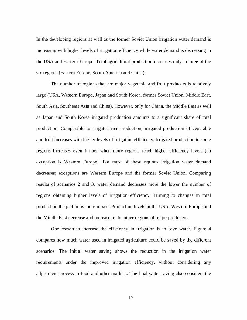
In the developing regions as well as the former Soviet Union irrigation water demand is
increasing with higher levels of irrigation efficiency while water demand is decreasing in
the USA and Eastern Europe. Total agricultural production increases only in three of the
six regions (Eastern Europe, South America and China).
The number of regions that are major vegetable and fruit producers is relatively
large (USA, Western Europe, Japan and South Korea, former Soviet Union, Middle East,
South Asia, Southeast Asia and China). However, only for China, the Middle East as well
as Japan and South Korea irrigated production amounts to a significant share of total
production. Comparable to irrigated rice production, irrigated production of vegetable
and fruit increases with higher levels of irrigation efficiency. Irrigated production in some
regions increases even further when more regions reach higher efficiency levels (an
exception is Western Europe). For most of these regions irrigation water demand
decreases; exceptions are Western Europe and the former Soviet Union. Comparing
results of scenarios 2 and 3, water demand decreases more the lower the number of
regions obtaining higher levels of irrigation efficiency. Turning to changes in total
production the picture is more mixed. Production levels in the USA, Western Europe and
the Middle East decrease and increase in the other regions of major producers.
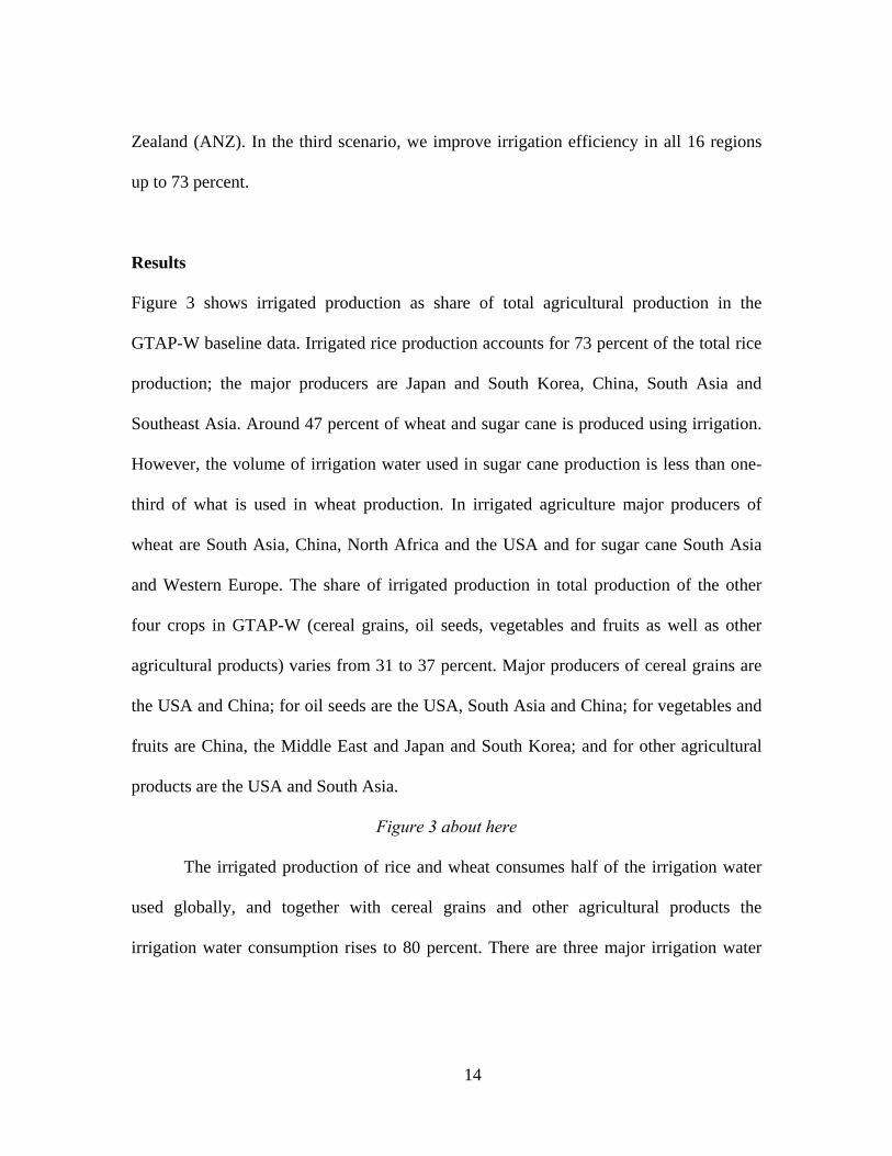
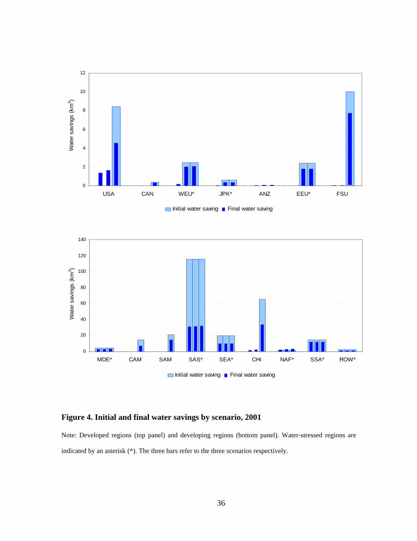
One reason to increase the efficiency in irrigation is to save water. Figure 4
compares how much water used in irrigated agriculture could be saved by the different
scenarios. The initial water saving shows the reduction in the irrigation water
requirements under the improved irrigation efficiency, without considering any
adjustment process in food and other markets. The final water saving also considers the
17
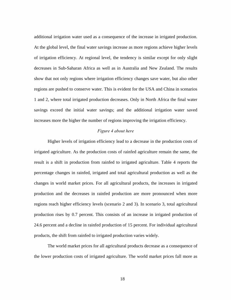
additional irrigation water used as a consequence of the increase in irrigated production.
At the global level, the final water savings increase as more regions achieve higher levels
of irrigation efficiency. At regional level, the tendency is similar except for only slight
decreases in Sub-Saharan Africa as well as in Australia and New Zealand. The results
show that not only regions where irrigation efficiency changes save water, but also other
regions are pushed to conserve water. This is evident for the USA and China in scenarios
1 and 2, where total irrigated production decreases. Only in North Africa the final water
savings exceed the initial water savings; and the additional irrigation water saved
increases more the higher the number of regions improving the irrigation efficiency.
Figure 4 about here
Higher levels of irrigation efficiency lead to a decrease in the production costs of
irrigated agriculture. As the production costs of rainfed agriculture remain the same, the
result is a shift in production from rainfed to irrigated agriculture. Table 4 reports the
percentage changes in rainfed, irrigated and total agricultural production as well as the
changes in world market prices. For all agricultural products, the increases in irrigated
production and the decreases in rainfed production are more pronounced when more
regions reach higher efficiency levels (scenario 2 and 3). In scenario 3, total agricultural
production rises by 0.7 percent. This consists of an increase in irrigated production of
24.6 percent and a decline in rainfed production of 15 percent. For individual agricultural
products, the shift from rainfed to irrigated production varies widely.
The world market prices for all agricultural products decrease as a consequence of
the lower production costs of irrigated agriculture. The world market prices fall more as
18
more regions improve irrigation efficiency. Lower market prices stimulate consumption
and total production of all agricultural products increases. In scenario 3, rice has the
greatest reduction in prices (-13.8 percent) which is accompanied by an increase in total
production (1.7 percent). The reduction in the world market price is the smallest for
cereals (-3.4 percent); total production rises by 0.4 percent.
Table 4 about here
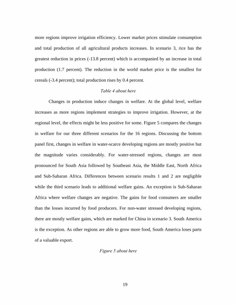
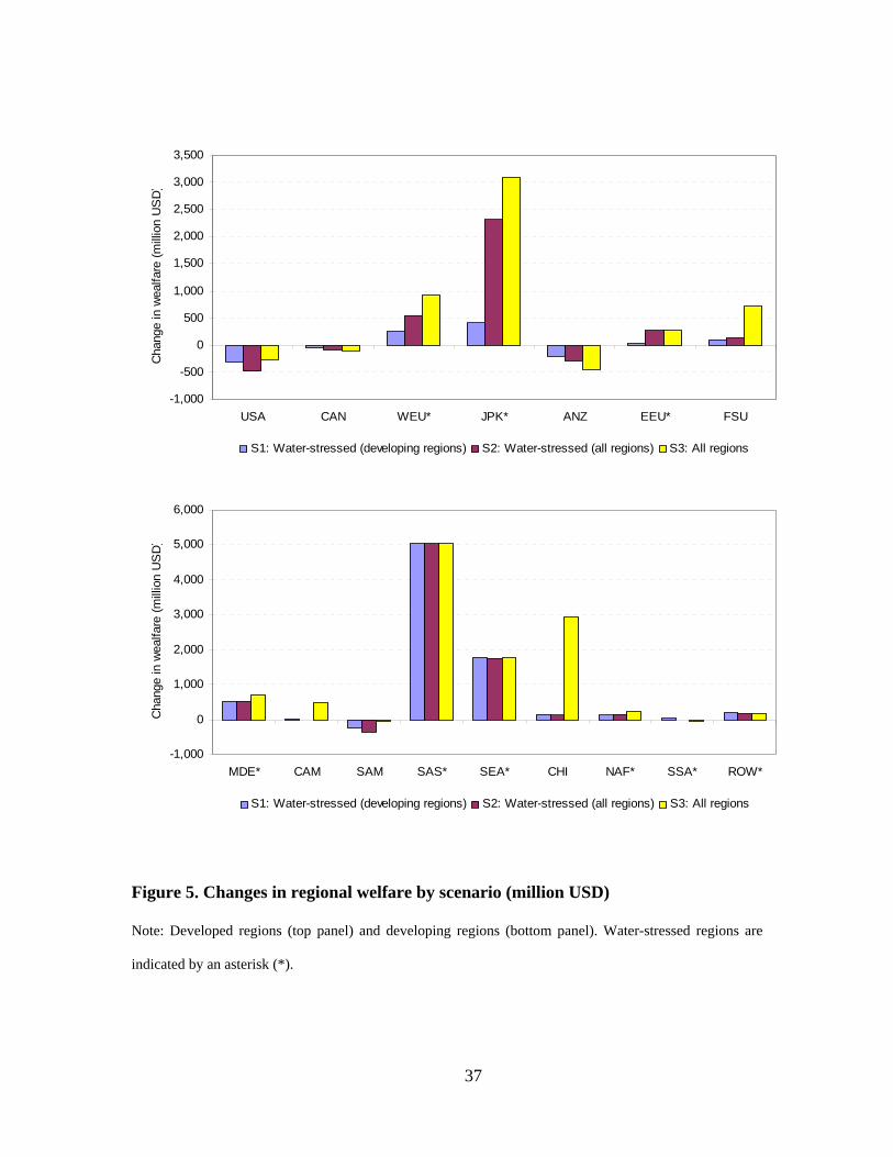
Changes in production induce changes in welfare. At the global level, welfare
increases as more regions implement strategies to improve irrigation. However, at the
regional level, the effects might be less positive for some. Figure 5 compares the changes
in welfare for our three different scenarios for the 16 regions. Discussing the bottom
panel first, changes in welfare in water-scarce developing regions are mostly positive but
the magnitude varies considerably. For water-stressed regions, changes are most
pronounced for South Asia followed by Southeast Asia, the Middle East, North Africa
and Sub-Saharan Africa. Differences between scenario results 1 and 2 are negligible
while the third scenario leads to additional welfare gains. An exception is Sub-Saharan
Africa where welfare changes are negative. The gains for food consumers are smaller
than the losses incurred by food producers. For non-water stressed developing regions,
there are mostly welfare gains, which are marked for China in scenario 3. South America
is the exception. As other regions are able to grow more food, South America loses parts
of a valuable export.
Figure 5 about here
19
The upper panel of figure 5 indicates that water-stressed developed regions
benefit from higher levels of irrigation efficiency, and even more so as efficiency
improvement occurs in more regions. This is also true for the non-water stressed former
Soviet Union. For food-exporters (USA, Canada, Australia and New Zealand) an
opposite effect occurs; the larger the number of regions implementing more efficient
irrigation management the greater the loss. This is reversed for the USA in scenario 3, in
which the USA itself also benefits from improved irrigation efficiency.
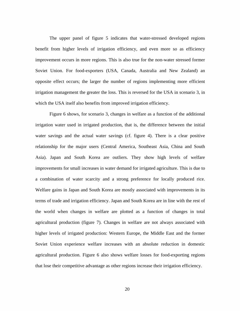
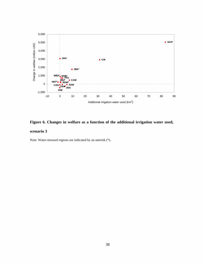
Figure 6 shows, for scenario 3, changes in welfare as a function of the additional
irrigation water used in irrigated production, that is, the difference between the initial
water savings and the actual water savings (cf. figure 4). There is a clear positive
relationship for the major users (Central America, Southeast Asia, China and South
Asia). Japan and South Korea are outliers. They show high levels of welfare
improvements for small increases in water demand for irrigated agriculture. This is due to
a combination of water scarcity and a strong preference for locally produced rice.
Welfare gains in Japan and South Korea are mostly associated with improvements in its
terms of trade and irrigation efficiency. Japan and South Korea are in line with the rest of
the world when changes in welfare are plotted as a function of changes in total
agricultural production (figure 7). Changes in welfare are not always associated with
higher levels of irrigated production: Western Europe, the Middle East and the former
Soviet Union experience welfare increases with an absolute reduction in domestic
agricultural production. Figure 6 also shows welfare losses for food-exporting regions
that lose their competitive advantage as other regions increase their irrigation efficiency.
20
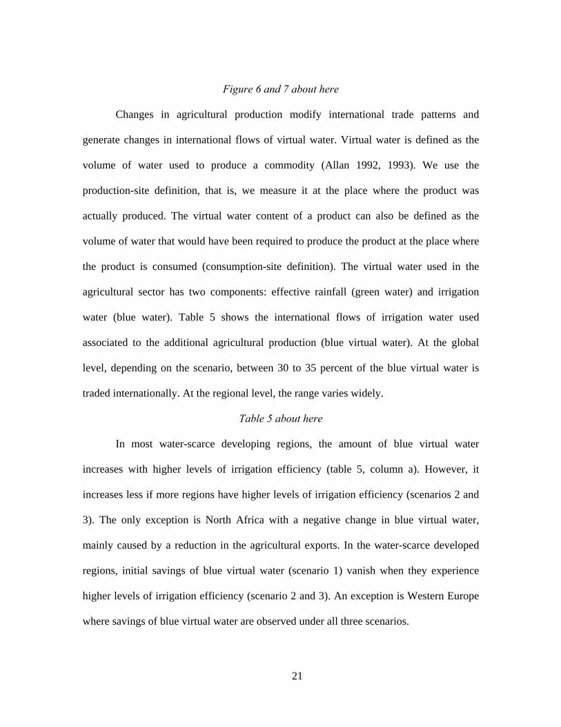
Figure 6 and 7 about here
Changes in agricultural production modify international trade patterns and
generate changes in international flows of virtual water. Virtual water is defined as the
volume of water used to produce a commodity (Allan 1992, 1993). We use the
production-site definition, that is, we measure it at the place where the product was
actually produced. The virtual water content of a product can also be defined as the
volume of water that would have been required to produce the product at the place where
the product is consumed (consumption-site definition). The virtual water used in the
agricultural sector has two components: effective rainfall (green water) and irrigation
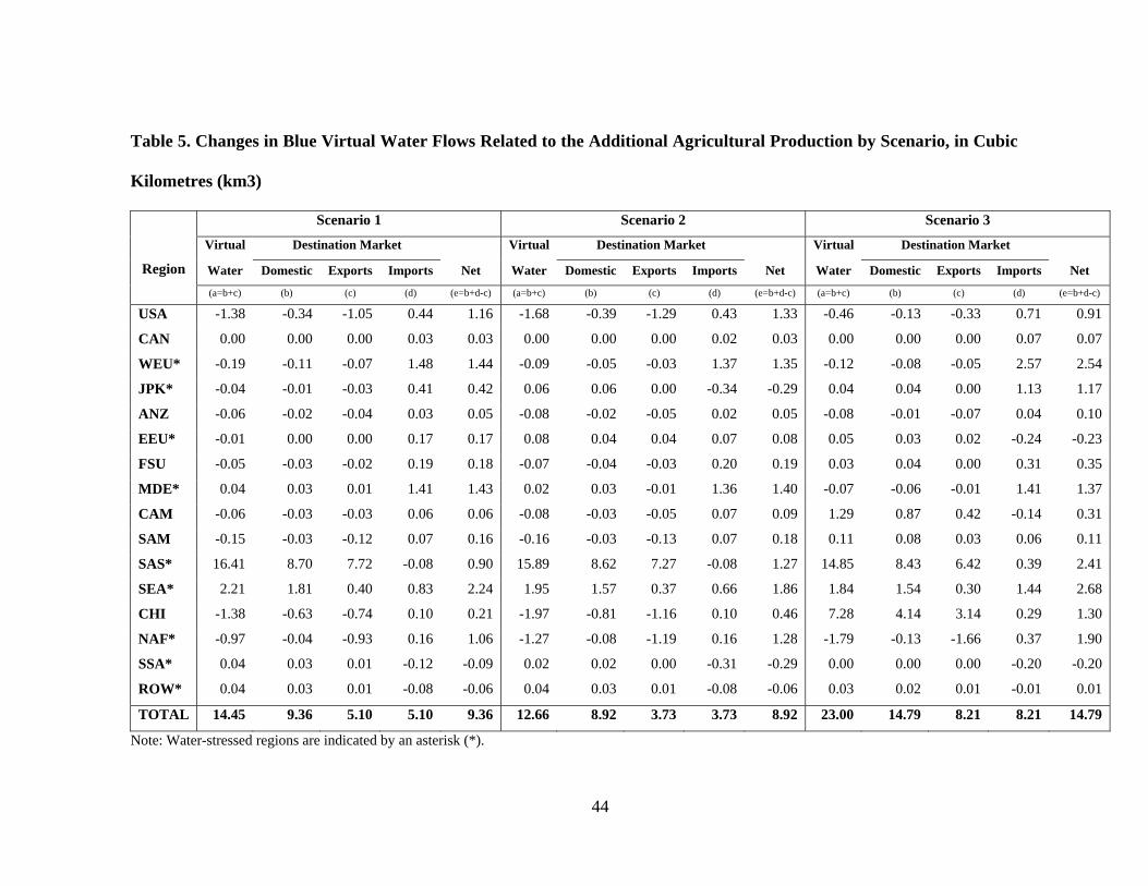
water (blue water). Table 5 shows the international flows of irrigation water used
associated to the additional agricultural production (blue virtual water). At the global
level, depending on the scenario, between 30 to 35 percent of the blue virtual water is
traded internationally. At the regional level, the range varies widely.
Table 5 about here
In most water-scarce developing regions, the amount of blue virtual water
increases with higher levels of irrigation efficiency (table 5, column a). However, it
increases less if more regions have higher levels of irrigation efficiency (scenarios 2 and
3). The only exception is North Africa with a negative change in blue virtual water,
mainly caused by a reduction in the agricultural exports. In the water-scarce developed
regions, initial savings of blue virtual water (scenario 1) vanish when they experience
higher levels of irrigation efficiency (scenario 2 and 3). An exception is Western Europe
where savings of blue virtual water are observed under all three scenarios.
21
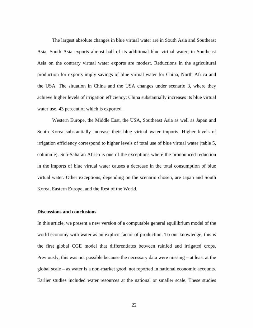
The largest absolute changes in blue virtual water are in South Asia and Southeast
Asia. South Asia exports almost half of its additional blue virtual water; in Southeast
Asia on the contrary virtual water exports are modest. Reductions in the agricultural
production for exports imply savings of blue virtual water for China, North Africa and
the USA. The situation in China and the USA changes under scenario 3, where they
achieve higher levels of irrigation efficiency; China substantially increases its blue virtual
water use, 43 percent of which is exported.
Western Europe, the Middle East, the USA, Southeast Asia as well as Japan and
South Korea substantially increase their blue virtual water imports. Higher levels of
irrigation efficiency correspond to higher levels of total use of blue virtual water (table 5,
column e). Sub-Saharan Africa is one of the exceptions where the pronounced reduction
in the imports of blue virtual water causes a decrease in the total consumption of blue
virtual water. Other exceptions, depending on the scenario chosen, are Japan and South
Korea, Eastern Europe, and the Rest of the World.
Discussions and conclusions
In this article, we present a new version of a computable general equilibrium model of the
world economy with water as an explicit factor of production. To our knowledge, this is
the first global CGE model that differentiates between rainfed and irrigated crops.
Previously, this was not possible because the necessary data were missing – at least at the
global scale – as water is a non-market good, not reported in national economic accounts.
Earlier studies included water resources at the national or smaller scale. These studies
22
necessarily miss the international dimension,6 which is important as water is implicitly
traded in international markets, mainly for agricultural products. In earlier studies by
ourselves, we had been unable to separate rainfed and irrigated agriculture.
Efforts towards improving irrigation management, e.g. through more efficient
irrigation methods, benefit societies by saving large amounts of water. These would be
available for other uses. In this article, we analyze if such a water policy would be
economically beneficial for the world as a whole as well as for individual countries and
whether and to what extent water savings could be achieved. We find that higher levels of
irrigation efficiency have, depending on the scenario and the region, a significant effect
on crop production, water use and welfare. Water use for some crops and some regions
goes up, and it goes down for other crops and regions. This leads to mixed pattern in total
water use for some regions.
At the global level, water savings are achieved and the magnitude increases when
more regions have higher levels of irrigation efficiency. The same tendency is observed
at the regional level, except for only slight decreases in Sub-Saharan Africa as well as in
Australia and New Zealand. The results show that not only regions where irrigation
efficiency changes are able to save water, but also other regions are pushed to conserve
water.
We find that welfare tends to increases with the additional irrigation water used in
irrigated production. The same positive relationship is observed when changes in welfare
are associated with changes in total agricultural production. However, increased water
efficiency also affects competitiveness, and hurts rainfed agriculture, so that there are
23
welfare losses as well. Such losses are more than offset, however, by the gains from
increased irrigated production and lower food prices.
Several limitations apply to the above results. First, in our analysis water-scarce
regions are defined based on country averages. We do not take into account that water
might be scarce within countries due to limited availability in water basins. China is an
example of such a country. Although on average water is not short, water supply is a
problem in Northern China. In fact, we implicitly assume a perfect water market in each
region. Second, in our analysis increases in irrigation efficiency are not accompanied by,
for example, changes in water prices. We implicitly assume that higher levels of
efficiency are possible with the current technology, at zero cost. Therefore, our scenarios
might overestimate the benefits of improved irrigation management. Third, we do not
consider individual options for irrigation management. Instead, we use water productivity
as a proxy for irrigation efficiency. These issues should be addressed in future research.
Future work will also study other issues, such as changes in water policy, and the effects
of climate change on water resources.
Acknowledgements
We had useful discussions about the topics of this article with Maria Berrittella, Beatriz
Gaitán, Siwa Msangi, Ramiro Parrado, Claudia Ringler, Mark Rosegrant, Roberto Roson,
Ken Strzepek, Timothy Sulser and Tingju Zhu. We are grateful to the IMPACT-WATER
people for making their data available to us. This article is supported by the Federal
Ministry for Economic Cooperation and Development, Germany under the project "Food
24
and Water Security under Global Change: Developing Adaptive Capacity with a Focus
on Rural Africa," which forms part of the CGIAR Challenge Program on Water and
Food, and by the Michael Otto Foundation for Environmental Protection.
25

Footnotes
1 The GTAP model is a standard CGE static model distributed with the GTAP database of the world
economy (www.gtap.org). For detailed information see Hertel (1997) and the technical references and
papers available on the GTAP website.
2 Burniaux and Truong (2002) developed a special variant of the model, called GTAP-E. The model is best
suited for the analysis of energy markets and environmental policies. There are two main changes in the
basic structure. First, energy factors are separated from the set of intermediate inputs and inserted in a
nested level of substitution with capital. This allows for more substitution possibilities. Second, database
and model are extended to account for CO2 emissions related to energy consumption.
3 See Annex 1 for the regional, sectoral and factoral aggregation used in GTAP-W.
4 The water-stressed countries were identified using the current AQUASTAT database.
5 Results for the other three agricultural sectors including oil seeds, sugar cane and sugar beet as well as
other agricultural products are excluded for clarity but can be obtained from the authors on request.
6 Although, in a single country CGE, there is either an explicit “Rest of the World” region or the rest of the
world is implicitly included in the closure rules.
26

References
Allan, J.A. 1992. “Fortunately there are substitutes for water otherwise our hydro-
political futures would be impossible.” In: Proceedings of the Conference on
Priorities for Water Resources Allocation and Management: Natural Resources and
Engineering Advisers Conference, Southampton, July 1992, pp. 13–26.
Allan, J.A. 1993. “Overall perspectives on countries and regions.” In: Rogers, P., Lydon,
P. (Eds.), Water in the Arab World: Perspectives and Prognoses. Cambridge, MA,
pp. 65–100.
Berrittella, M., A.Y. Hoekstra, K. Rehdanz, R. Roson, and R.S.J. Tol. 2007. “The
Economic Impact of Restricted Water Supply: A Computable General Equilibrium
Analysis.” Water Research 41: 1799-1813.
Berrittella, M., K. Rehdanz, R. Roson, and R.S.J. Tol. Forthcoming, a. “The Economic
Impact of Water Pricing: A Computable General Equilibrium Analysis.” Water
Policy, in press.
Berrittella, M., K. Rehdanz, and R.S.J. Tol. 2006. “The Economic Impact of the South-
North Water Transfer Project in China: A Computable General Equilibrium
Analysis.” Research unit Sustainability and Global Change FNU-117, Hamburg
University and Centre for Marine and Atmospheric Science, Hamburg.
Berrittella, M., K. Rehdanz, R.S.J. Tol, and Y. Zhang. Forthcoming, b. “The Impact of
Trade Liberalisation on Water Use: A Computable General Equilibrium Analysis.”
Journal of Economic Integration, in press.
27
Bluemling, B., H. Yang, and C. Pahl-Wostl. 2007. “Making water productivity
operational-A concept of agricultural water productivity exemplified at a wheat-
maize cropping pattern in the North China plain.” Agricultural Water Management
91: 11-23.
Burniaux, J.M. and T.P. Truong. 2002. “GTAP-E: An Energy Environmental Version of
the GTAP Model.” GTAP Technical Paper no. 16.
Burt, C.M., A.J. Clemmens, T.S. Strelkoff, K.H. Solomon, R.D. Bliesner, R.A. Hardy,
T.A. Howell, and D.E. Eisenhauer. 1997. “Irrigation performance measures:
Efficiency and uniformity.” Journal of Irrigation and Drainage Engineering 123:
423-442.
Decaluwé, B., A. Patry, and L. Savard. 1999. “When water is no longer heaven sent:
Comparative pricing analysis in a AGE model.” Working Paper 9908, CRÉFA 99-05,
Départment d’économique, Université Laval.
Deng, X., L. Shan, L. Zhang, and N.C. Turner. 2006. “Improving agricultural water use
efficiency in arid and semiarid areas of China.” Agricultural Water Management 80:
23-40.
Diao, X., and T. Roe. 2003. “Can a water market avert the “double-whammy” of trade
reform and lead to a “win-win” outcome?” Journal of Environmental Economics and
Management 45: 708-723.
Dinar, A., and D. Yaron. 1992. “Adoption and Abandonment of Irrigation Technologies.”
Agricultural Economics 6: 315-32.
28
Easter, K.W., and Y. Liu. 2005. “Cost Recovery and Water Pricing for Irrigation and
Drainage Projects.” Agriculture and Rural Development Discussion Paper 26. The
World Bank, Washington, D.C.
Ettouney, H.M., H.T. El-Dessouky, R.S. Faibish, and P.J. Gowin. 2002. “Evaluating the
Economics of Desalination.” Chemical Engineering Progress, December 2002, pp.
32-39.
FAO. 2001. Handbook on pressurized irrigation techniques. Rome, FAO.
Feng, S., L.X. Li, Z.G. Duan, and J.L. Zhang. 2007. “Assessing the impacts of South-to-
North Water Transfer Project with decision support systems.” Decision Support
Systems 42 (4): 1989-2003.
Fraiture, C. de, X. Cai, U. Amarasinghe, M. Rosegrant, and D. Molden. 2004. “Does
international cereal trade save water? The impact of virtual water trade on global
water use.” Comprehensive Assessment Research Report 4, Colombo, Sri Lanka.
Gómez, C.M., D. Tirado, and J. Rey-Maquieira. 2004. “Water exchange versus water
work: Insights from a computable general equilibrium model for the Balearic
Islands.” Water Resources Research 42 W10502 10.1029/2004WR003235.
Goodman, D.J. 2000. “More reservoir or transfer? A computable general equilibrium
analysis of projected water shortages in the Arkansas River Basin.” Journal of
Agricultural and Resource Economics 25 (2): 698-713.
Hertel, T.W. 1997. Global Trade Analysis: Modeling and Applications. Cambridge
University Press, Cambridge.
Jensen, M.E. 2007. “Beyond efficiency.” Irrigation Science 25 (3): 233-245.
29
Johansson, R.C., Y. Tsur, T.L. Roe, R. Doukkali, and A. Dinar. 2002. “Pricing irrigation
water: a review of theory and practice.” Water Policy 4 (2): 173-199.
Kamara, A. B., and H. Sally. 2004. “Water management options for food security in
South Africa: scenarios, simulations and policy implications.” Development Southern
Africa 21 (2): 365-384.
Lee, H., J. Oliveira-Martins, and D. van der Mensbrugghe. 1994. “The OECD GREEN
Model: An updated overview.” Working Paper No. 97, OECD, Paris.
Letsoalo, A., J. Blignaut, T. de Wet, M. de Wit, S. Hess, R.S.J. Tol and J. van Heerden.
2007. “Triple Dividends of Water Consumption Charges in South Africa.” Water
Resources Research, 43, W05412.
Lilienfeld, A. and M. Asmild. 2007. “Estimation of excess water use in irrigated
agriculture: A Data Envelopment Analysis approach.” Agricultural Water
Management 94 (1-3): 73-82.
Mailhol, J. C., A. Zairi, A. Slatni, B. Ben Nouma, and H. El Amani. 2004. “Analysis of
irrigation systems and irrigation strategies for durum wheat in Tunisia.” Agricultural
Water Management 70 (1): 19-37.
McDonald, S., S. Robinson, and K. Thierfelder. 2005. “A SAM Based Global CGE
Model using GTAP Data.” Sheffield Economics Research Paper 2005:001. The
University of Sheffield.
Pereira, L.S. 1999. “Higher performance through combined improvements in irrigation
methods and scheduling: a discussion.” Agricultural Water Management 40 (2-3):
153-169.
30
Pereira, L.S., T. Oweis, and A. Zairi. 2002. “Irrigation management under water
scarcity.” Agricultural Water Management 57 (3): 175-206.
Qadir, M., B.R. Sharma, A. Bruggeman, R. Choukr-Allah, and F. Karajeh. 2007. “Non-
conventional water resources and opportunities for water augmentation to achieve
food security in water scarce countries.” Agricultural Water Management 87 (1): 2-
22.
Rosegrant, M.W., X. Cai, and S.A. Cline. 2002. World Water and Food to 2025: Dealing
With Scarcity. International Food Policy Research Institute. Washington, DC.
Seckler, D., D. Molden, and R. Barker. 1998. “World Water Demand and Supply, 1990
to 2025: Scenarios and Issues.” International Water Management Report, Research
Report 19.
Seung, C.K., T.R. Harris, J.E. Eglin, and N.R. Netusil. 2000. “Impacts of water
reallocation: A combined computable general equilibrium and recreation demand
model approach.” The Annals of Regional Science 34: 473-487.
Strzepek, K.M., G.W. Yohe, R.S.J. Tol and M. Rosegrant. Forthcoming. “The Value of
the High Aswan Dam to the Egyptian Economy.” Ecological Economics, in press.
Tsur, Y., A. Dinar, R. Doukkali, and T. Roe. 2004. “Irrigation water pricing: policy
implications based on international comparison.” Environmental and Development
Economics 9: 735-755.
United Nations. 1993. The System of National Accounts (SNA93). United Nations, New
York.
31
Van Heerden, J.H., J.N. Blignaut, and M. Horridge. Forthcoming. “Integrated water and
economic modelling of the impacts of water market instruments on the South African
economy.” Ecological Economics, in press.
Wichelns, D. 2003. “Enhancing water policy discussions by including analysis of non-
water inputs and farm-level constraints.” Agricultural Water Management 62 (2): 93-
103.
Yang, H., X. Zhang, and A.J.B. Zehnder. 2003. “Water scarcity, pricing mechanism and
institutional reform in northern China irrigated agriculture.” Agricultural Water
Management 61 (2): 143-161.
Zhou, Y. and R.S.J. Tol. 2005. “Evaluating the costs of desalination and water transport.”
Water Resource Research 41(3) W03003 10.1029/2004WR003749.
32
Capital Energy Composite
σKE
Irrigated Land-Water Rainfed Pasture Natural Labor Capital-Energy Composite Land Land Resources Composite
Region 1 … Region r
σM
Domestic Foreign
σD
Irrigated Irrigation Land
σLW
σVAE
σ = 0
Value-added (Including energy inputs)
All other inputs (Excluding energy inputs but including energy feedstock)
Output
Figure 1. Nested tree structure for industrial production process in GTAP-W
(truncated)
Note: The original land endowment has been split into pasture land, rainfed land, irrigated land and
irrigation (bold letters).
33
Irrigation efficiency(Percentage)
40 - 4647 - 5354 - 5960 - 6667 - 73
Figure 2. Average irrigation efficiency, 2001 baseline data
34
0
10
20
30
40
50
60
70
80
Rice (321 km3)
Wheat (296 Km3)
OthAgr (222 km3)
CerCrops(221 Km3)
SugCan (89 km3)
VegFruits(82 km3)
OilSeeds(79 km3)
Per
cent
SAS* (485 km3)CHI (278 km3)USA (190 km3)MDE* (62 km3)SEA* (56 km3)SAM (47 km3)FSU (47 km3)CAM (46 km3)NAF* (42 km3)SSA* (37 km3)ANZ (15 km3)EEU* (14 km3)WEU* (10 km3)ROW* (5 km3)JPK* (3 Km3)CAN (1 km3)
Figure 3. Share of irrigated production in total production by crop and region, 2001
baseline data
Note: Irrigation water used in km3 by crop and region is shown in parenthesis. Water-stressed regions are
indicated by an asterisk (*).
35
0
2
4
6
8
10
12
USA CAN WEU* JPK* ANZ EEU* FSU
Wat
er s
avin
gs (k
m 3 )
Initial water saving Final water saving
0
20
40
60
80
100
120
140
MDE* CAM SAM SAS* SEA* CHI NAF* SSA* ROW*
Wat
er s
avin
gs (k
m 3 )
Initial water saving Final water saving
Figure 4. Initial and final water savings by scenario, 2001
Note: Developed regions (top panel) and developing regions (bottom panel). Water-stressed regions are
indicated by an asterisk (*). The three bars refer to the three scenarios respectively.
36
-1,000
-500
0
500
1,000
1,500
2,000
2,500
3,000
3,500
USA CAN WEU* JPK* ANZ EEU* FSU
Cha
nge
in w
ealfa
re (m
illio
n U
SD
)
S1: Water-stressed (developing regions) S2: Water-stressed (all regions) S3: All regions
-1,000
0
1,000
2,000
3,000
4,000
5,000
6,000
MDE* CAM SAM SAS* SEA* CHI NAF* SSA* ROW*
Cha
nge
in w
ealfa
re (m
illio
n U
SD
)
S1: Water-stressed (developing regions) S2: Water-stressed (all regions) S3: All regions
Figure 5. Changes in regional welfare by scenario (million USD)
Note: Developed regions (top panel) and developing regions (bottom panel). Water-stressed regions are
indicated by an asterisk (*).
37
ANZUSA
MDE*
NAF*CAM
SEA*
JPK* CHI
SAS*
WEU*FSU
ROW*EEU*
SSA*SAMCAN
-1,000
0
1,000
2,000
3,000
4,000
5,000
6,000
-10 0 10 20 30 40 50 60 70 80 90
Additional irrigation water used (km3)
Cha
nge
in w
elfa
re (m
illio
n U
SD
)
Figure 6. Changes in welfare as a function of the additional irrigation water used,
scenario 3
Note: Water-stressed regions are indicated by an asterisk (*).
38
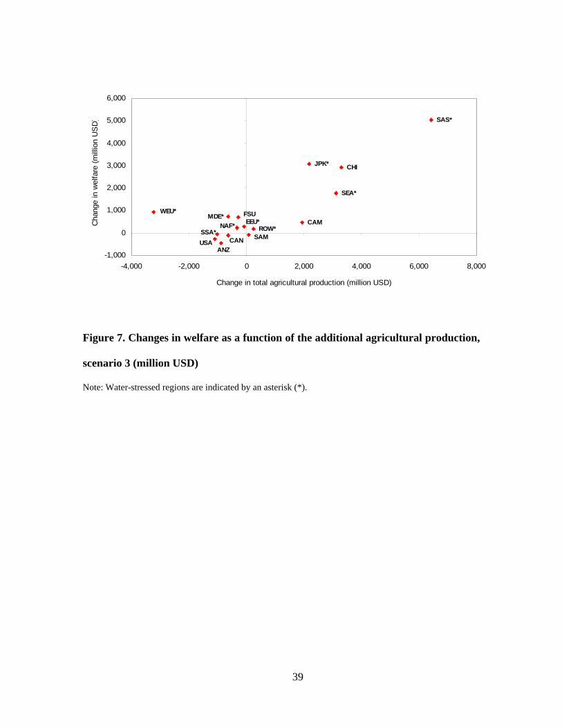
Note: Water-stressed regions are indicated by an asterisk (*).
Figure 7. Changes in welfare as a function of the additional agricultural production,
scenario 3 (million USD)
ANZUSA
SAMCAN
-1,000-4,000 -2,000 0 2
Change in total agricultu
MDE*NAF* CAM
SEA*
JPK* CHI
SAS*
WEU* FSU
ROW*EEU*
SSA*0
1,000
2,000
3,000
4,000
5,000
6,000
,000 4,000 6,000 8,000
ral production (million USD)
Cha
nge
in w
elfa
re (m
illio
n U
SD
)
39
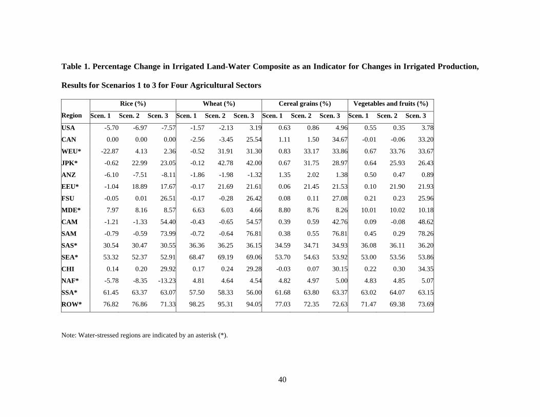
Table 1. Percentage Change in Irrigated Land-Water Composite as an Indicator for Changes in Irrigated Production,
Results for Scenarios 1 to 3 for Four Agricultural Sectors
Rice (%) Wheat (%) Cereal grains (%) Vegetables and fruits (%)
Region Scen. 1 Scen. 2 Scen. 3 Scen. 1 Scen. 2 Scen. 3 Scen. 1 Scen. 2 Scen. 3 Scen. 1 Scen. 2 Scen. 3
USA -5.70 -6.97 -7.57 -1.57 -2.13 3.19 0.63 0.86 4.96 0.55 0.35 3.78
CAN 0.00 0.00 0.00 -2.56 -3.45 25.54 1.11 1.50 34.67 -0.01 -0.06 33.20
WEU* -22.87 4.13 2.36 -0.52 31.91 31.30 0.83 33.17 33.86 0.67 33.76 33.67
JPK* -0.62 22.99 23.05 -0.12 42.78 42.00 0.67 31.75 28.97 0.64 25.93 26.43
ANZ -6.10 -7.51 -8.11 -1.86 -1.98 -1.32 1.35 2.02 1.38 0.50 0.47 0.89
EEU* -1.04 18.89 17.67 -0.17 21.69 21.61 0.06 21.45 21.53 0.10 21.90 21.93
FSU -0.05 0.01 26.51 -0.17 -0.28 26.42 0.08 0.11 27.08 0.21 0.23 25.96
MDE* 7.97 8.16 8.57 6.63 6.03 4.66 8.80 8.76 8.26 10.01 10.02 10.18
CAM -1.21 -1.33 54.40 -0.43 -0.65 54.57 0.39 0.59 42.76 0.09 -0.08 48.62
SAM -0.79 -0.59 73.99 -0.72 -0.64 76.81 0.38 0.55 76.81 0.45 0.29 78.26
SAS* 30.54 30.47 30.55 36.36 36.25 36.15 34.59 34.71 34.93 36.08 36.11 36.20
SEA* 53.32 52.37 52.91 68.47 69.19 69.06 53.70 54.63 53.92 53.00 53.56 53.86
CHI 0.14 0.20 29.92 0.17 0.24 29.28 -0.03 0.07 30.15 0.22 0.30 34.35
NAF* -5.78 -8.35 -13.23 4.81 4.64 4.54 4.82 4.97 5.00 4.83 4.85 5.07
SSA* 61.45 63.37 63.07 57.50 58.33 56.00 61.68 63.80 63.37 63.02 64.07 63.15
ROW* 76.82 76.86 71.33 98.25 95.31 94.05 77.03 72.35 72.63 71.47 69.38 73.69
Note: Water-stressed regions are indicated by an asterisk (*).
40
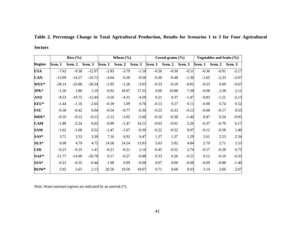
Table 2. Percentage Change in Total Agricultural Production, Results for Scenarios 1 to 3 for Four Agricultural
Sectors
Rice (%) Wheat (%) Cereal grains (%) Vegetables and fruits (%)
Region Scen. 1 Scen. 2 Scen. 3 Scen. 1 Scen. 2 Scen. 3 Scen. 1 Scen. 2 Scen. 3 Scen. 1 Scen. 2 Scen. 3
USA -7.62 -9.38 -12.97 -2.83 -3.79 -1.18 -0.26 -0.30 -0.51 -0.36 -0.91 -2.17
CAN -13.89 -14.27 -16.73 -4.64 -6.30 -9.56 -0.30 -0.48 -1.36 -1.65 -2.33 -2.07
WEU* -28.14 -25.86 -28.34 -1.95 -1.26 -3.03 -0.33 -0.19 -0.81 -0.53 0.69 -0.67
JPK* -1.50 1.80 1.10 -0.92 18.97 17.35 0.00 10.88 7.38 -0.08 2.38 2.11
ANZ -8.53 -10.75 -12.44 -3.56 -4.31 -4.59 0.21 0.37 -1.47 -0.83 -1.51 -2.13
EEU* -1.44 -1.16 -2.65 -0.39 1.09 0.76 -0.13 0.27 0.11 -0.08 0.74 0.52
FSU -0.38 -0.42 0.04 -0.54 -0.77 -0.30 -0.25 -0.33 -0.13 -0.08 -0.17 0.53
MDE* -0.10 -0.12 -0.13 -2.12 -3.02 -5.00 -0.10 -0.38 -1.40 0.47 0.24 -0.05
CAM -1.89 -2.24 6.03 -0.99 -1.47 14.11 -0.03 -0.01 3.26 -0.37 -0.79 6.17
SAM -1.62 -1.68 0.52 -1.47 -1.67 -0.30 -0.22 -0.32 0.07 -0.12 -0.58 1.40
SAS* 3.71 3.53 3.30 7.16 6.92 6.47 1.37 1.37 1.29 2.61 2.53 2.34
SEA* 6.08 4.79 4.75 14.56 14.54 13.93 5.63 5.82 4.84 2.79 2.71 2.53
CHI -0.23 -0.35 1.41 -0.21 -0.31 2.16 -0.45 -0.52 2.74 -0.17 -0.28 0.75
NAF* -11.77 -14.90 -20.78 0.17 -0.27 -0.88 0.33 0.26 -0.21 0.12 -0.10 -0.35
SSA* -0.22 -0.35 -0.44 1.98 0.99 -0.68 0.07 0.06 -0.08 -0.09 -0.88 -1.40
ROW* 5.92 5.61 2.13 20.56 19.50 18.07 0.71 0.68 0.03 3.14 2.66 2.07
Note: Water-stressed regions are indicated by an asterisk (*).
41
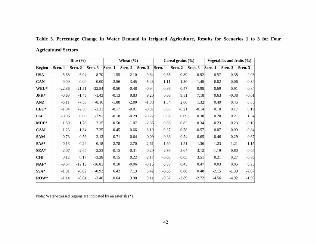
Table 3. Percentage Change in Water Demand in Irrigated Agriculture, Results for Scenarios 1 to 3 for Four
Agricultural Sectors
Rice (%) Wheat (%) Cereal grains (%) Vegetables and fruits (%)
Region Scen. 1 Scen. 2 Scen. 3 Scen. 1 Scen. 2 Scen. 3 Scen. 1 Scen. 2 Scen. 3 Scen. 1 Scen. 2 Scen. 3
USA -5.68 -6.94 -8.70 -1.55 -2.10 0.64 0.65 0.89 -0.92 0.57 0.38 -2.03
CAN 0.00 0.00 0.00 -2.56 -3.45 -5.43 1.11 1.50 1.45 -0.02 -0.06 0.34
WEU* -22.86 -21.51 -22.84 -0.50 -0.48 -0.94 0.86 0.47 0.98 0.69 0.91 0.84
JPK* -0.63 -1.45 -1.43 -0.13 9.83 9.20 0.66 9.51 7.18 0.63 -0.38 -0.01
ANZ -6.11 -7.53 -8.16 -1.88 -2.00 -1.38 1.34 2.00 1.32 0.49 0.45 0.83
EEU* -1.04 -2.30 -3.31 -0.17 -0.01 -0.07 0.06 -0.21 -0.14 0.10 0.17 0.19
FSU -0.06 0.00 -2.91 -0.18 -0.29 -0.22 0.07 0.09 0.38 0.20 0.21 1.34
MDE* 1.60 1.78 2.15 -0.50 -1.07 -2.36 0.86 0.82 0.34 -0.23 -0.23 -0.10
CAM -1.23 -1.34 -7.25 -0.45 -0.66 8.10 0.37 0.58 -0.57 0.07 -0.09 -0.84
SAM -0.78 -0.59 -2.12 -0.71 -0.64 -0.09 0.38 0.54 0.65 0.46 0.29 0.67
SAS* -0.18 -0.24 -0.18 2.78 2.70 2.61 -1.60 -1.51 -1.36 -1.23 -1.21 -1.15
SEA* -2.07 -2.65 -2.33 -0.15 0.31 0.20 2.98 3.64 3.12 -1.19 -0.80 -0.65
CHI 0.12 0.17 -3.28 0.15 0.22 2.17 -0.05 0.05 3.51 0.21 0.27 -0.86
NAF* -9.67 -12.13 -16.81 0.10 -0.06 -0.15 0.30 0.45 0.47 0.03 0.05 0.25
SSA* -1.91 -0.62 -0.92 6.42 7.13 5.42 -0.56 0.88 0.48 -2.15 -1.39 -2.07
ROW* -1.14 -0.04 -3.40 10.64 9.90 9.11 -0.67 -2.89 -2.72 -4.56 -4.92 -1.96
Note: Water-stressed regions are indicated by an asterisk (*).
42

Table 4. Percentage Change in Global Total, Irrigated and Rainfed Agricultural Production and World Market Prices
by Scenario
Scenario 1 Scenario 2 Scenario 3
Agricultural Agricultural production Agricultural production Agricultural production
products Total Irrigated Rainfed Price Total Irrigated Rainfed Price Total Irrigated Rainfed Price
Rice 1.07 14.74 -36.08 -6.78 1.55 17.49 -41.75 -10.03 1.71 19.69 -47.16 -13.79
Wheat 0.45 13.22 -11.03 -2.95 0.73 17.22 -14.09 -3.60 0.87 24.58 -20.45 -5.16
Cereal grains 0.07 4.35 -2.29 -0.95 0.13 7.34 -3.84 -1.34 0.38 21.94 -11.49 -3.44
Vegetable and fruits 0.25 7.38 -3.59 -1.41 0.41 15.46 -7.68 -2.44 0.70 29.01 -14.52 -4.47
Oil seeds 0.58 15.96 -6.36 -2.57 0.62 16.90 -6.73 -2.78 1.00 27.97 -11.18 -4.19
Sugar cane and beet 0.76 21.52 -17.59 -6.26 0.80 26.69 -22.09 -6.87 0.90 37.49 -31.45 -8.25
Other agri. products 0.27 8.83 -4.78 -1.91 0.39 12.72 -6.87 -2.47 0.48 21.43 -11.86 -3.99
TOTAL 0.35 10.02 -6.02 0.52 14.86 -8.93 0.71 24.58 -15.00
43
44
Table 5. Changes in Blue Virtual Water Flows Related to the Additional Agricultural Production by Scenario, in Cubic
Kilometres (km3)
Scenario 1 Scenario 2 Scenario 3
Virtual Destination Market Virtual Destination Market Virtual Destination Market
Region Water Domestic Exports Imports Net Water Domestic Exports Imports Net Water Domestic Exports Imports Net
(a=b+c) (b) (c) (d) (e=b+d-c) (a=b+c) (b) (c) (d) (e=b+d-c) (a=b+c) (b) (c) (d) (e=b+d-c)
USA -1.38 -0.34 -1.05 0.44 1.16 -1.68 -0.39 -1.29 0.43 1.33 -0.46 -0.13 -0.33 0.71 0.91
CAN 0.00 0.00 0.00 0.03 0.03 0.00 0.00 0.00 0.02 0.03 0.00 0.00 0.00 0.07 0.07
WEU* -0.19 -0.11 -0.07 1.48 1.44 -0.09 -0.05 -0.03 1.37 1.35 -0.12 -0.08 -0.05 2.57 2.54
JPK* -0.04 -0.01 -0.03 0.41 0.42 0.06 0.06 0.00 -0.34 -0.29 0.04 0.04 0.00 1.13 1.17
ANZ -0.06 -0.02 -0.04 0.03 0.05 -0.08 -0.02 -0.05 0.02 0.05 -0.08 -0.01 -0.07 0.04 0.10
EEU* -0.01 0.00 0.00 0.17 0.17 0.08 0.04 0.04 0.07 0.08 0.05 0.03 0.02 -0.24 -0.23
FSU -0.05 -0.03 -0.02 0.19 0.18 -0.07 -0.04 -0.03 0.20 0.19 0.03 0.04 0.00 0.31 0.35
MDE* 0.04 0.03 0.01 1.41 1.43 0.02 0.03 -0.01 1.36 1.40 -0.07 -0.06 -0.01 1.41 1.37
CAM -0.06 -0.03 -0.03 0.06 0.06 -0.08 -0.03 -0.05 0.07 0.09 1.29 0.87 0.42 -0.14 0.31
SAM -0.15 -0.03 -0.12 0.07 0.16 -0.16 -0.03 -0.13 0.07 0.18 0.11 0.08 0.03 0.06 0.11
SAS* 16.41 8.70 7.72 -0.08 0.90 15.89 8.62 7.27 -0.08 1.27 14.85 8.43 6.42 0.39 2.41
SEA* 2.21 1.81 0.40 0.83 2.24 1.95 1.57 0.37 0.66 1.86 1.84 1.54 0.30 1.44 2.68
CHI -1.38 -0.63 -0.74 0.10 0.21 -1.97 -0.81 -1.16 0.10 0.46 7.28 4.14 3.14 0.29 1.30
NAF* -0.97 -0.04 -0.93 0.16 1.06 -1.27 -0.08 -1.19 0.16 1.28 -1.79 -0.13 -1.66 0.37 1.90
SSA* 0.04 0.03 0.01 -0.12 -0.09 0.02 0.02 0.00 -0.31 -0.29 0.00 0.00 0.00 -0.20 -0.20
ROW* 0.04 0.03 0.01 -0.08 -0.06 0.04 0.03 0.01 -0.08 -0.06 0.03 0.02 0.01 -0.01 0.01
TOTAL 14.45 9.36 5.10 5.10 9.36 12.66 8.92 3.73 3.73 8.92 23.00 14.79 8.21 8.21 14.79
Note: Water-stressed regions are indicated by an asterisk (*).
Annex I: Aggregations in GTAP-W
A. Regional Aggregation B. Sectoral Aggregation
1. USA - United States 1. Rice – Rice
2. CAN - Canada 2. Wheat - Wheat
3. WEU - Western Europe 3. CerCrops - Cereal grains
4. JPK - Japan and South Korea 4. VegFruits - Vegetable, fruits, nuts
5. ANZ - Australia and New Zealand 5. OilSeeds - Oil seeds
6. EEU - Eastern Europe 6. Sug_Can - Sugar cane, sugar beet
7. FSU - Former Soviet Union 7. Oth_Agr - Other agricultural products
8. MDE - Middle East 8. Animals - Animals
9. CAM - Central America 9. Meat - Meat
10. SAM - South America 10. Food_Prod - Food products
11. SAS - South Asia 11. Forestry - Forestry
12. SEA - Southeast Asia 12. Fishing - Fishing
13. CHI - China 13. Coal - Coal
14. NAF - North Africa 14. Oil – Oil
15. SSA - Sub-Saharan Africa 15. Gas – Gas
16. ROW - Rest of the World 16. Oil_Pcts - Oil products
17. Electricity - Electricity
C. Endowments 18. Water - Water
Wtr - Irrigation 19. En_Int_Ind - Energy intensive industries
Lnd - Irrigated land 20. Oth_Ind - Other industry and services
RfLand - Rainfed land 21. Mserv - Market services
PsLand - Pasture land 22. NMServ - Non-market services
Lab - Labour
Capital - Capital
NatlRes - Natural resources
45
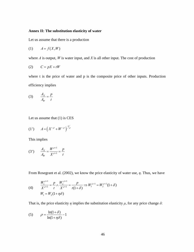
Annex II: The substitution elasticity of water
Let us assume that there is a production
(1) ( , )A f X W=
where A is output, W is water input, and X is all other input. The cost of production
(2) C pX tW= +
where t is the price of water and p is the composite price of other inputs. Production
efficiency implies
(3) X
W
A pA t
=
Let us assume that (1) is CES
(1’) ( )1
A X Wρ ρ ρ−
− −= +
This implies
(3’) 1
1X
W
A W pA X t
ρ
ρ
+
+= =
From Rosegrant et al. (2002), we know the price elasticity of water use, η. Thus, we have
(4)
1 11 11 2
1 21 1
1 2
(1 )(1 )
(1 )
W p W p W WX t X t
W W
ρ ρρ ρ
ρ ρ δδ
ηδ
+ ++ +
+ += ∧ = ⇒ = ++
= +
That is, the price elasticity η implies the substitution elasticity ρ, for any price change δ:
(5) ln(1 ) 1ln(1 )
δρηδ+
= −+
46


