Vibration Testing

Vibration Testing Equipment

For vibration testing, you need• an excitation source• a device to measure the response• a digital signal processor to analyze the system response

Excitation sources

Typically either instrumented hammers or shakers are used.

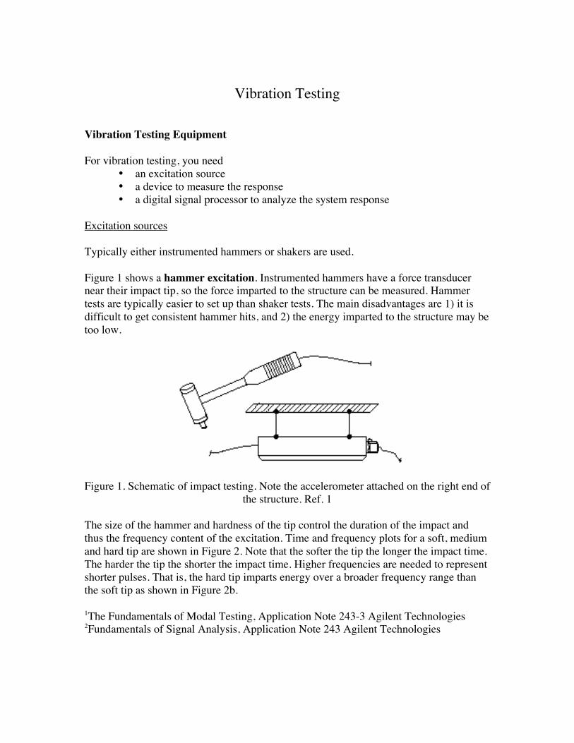
Figure 1 shows a hammer excitation. Instrumented hammers have a force transducernear their impact tip, so the force imparted to the structure can be measured. Hammertests are typically easier to set up than shaker tests. The main disadvantages are 1) it isdifficult to get consistent hammer hits, and 2) the energy imparted to the structure may betoo low.

Figure 1. Schematic of impact testing. Note the accelerometer attached on the right end ofthe structure. Ref. 1

The size of the hammer and hardness of the tip control the duration of the impact andthus the frequency content of the excitation. Time and frequency plots for a soft, mediumand hard tip are shown in Figure 2. Note that the softer the tip the longer the impact time.The harder the tip the shorter the impact time. Higher frequencies are needed to representshorter pulses. That is, the hard tip imparts energy over a broader frequency range thanthe soft tip as shown in Figure 2b.

1The Fundamentals of Modal Testing, Application Note 243-3 Agilent Technologies2Fundamentals of Signal Analysis, Application Note 243 Agilent Technologies

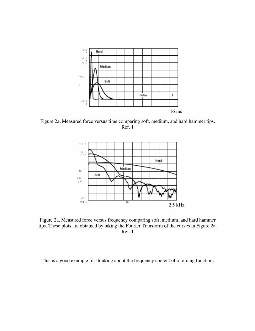
Figure 2a. Measured force versus time comparing soft, medium, and hard hammer tips.Ref. 1

Figure 2a. Measured force versus frequency comparing soft, medium, and hard hammertips. These plots are obtained by taking the Fourier Transform of the curves in Figure 2a.

Ref. 1

This is a good example for thinking about the frequency content of a forcing function.

16 ms

2.5 kHz

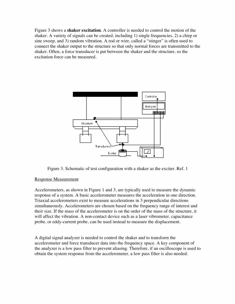
Figure 3 shows a shaker excitation. A controller is needed to control the motion of theshaker. A variety of signals can be created, including 1) single frequencies, 2) a chirp orsine sweep, and 3) random vibration. A rod or wire, called a “stinger” is often used toconnect the shaker output to the structure so that only normal forces are transmitted to theshaker. Often, a force transducer is put between the shaker and the structure, so theexcitation force can be measured.

Figure 3. Schematic of test configuration with a shaker as the exciter. Ref. 1

Response Measurement

Accelerometers, as shown in Figure 1 and 3, are typically used to measure the dynamicresponse of a system. A basic accelerometer measures the acceleration in one direction.Triaxial accelerometers exist to measure accelerations in 3 perpendicular directionssimultaneously. Accelerometers are chosen based on the frequency range of interest andtheir size. If the mass of the accelerometer is on the order of the mass of the structure, itwill affect the vibration. A non-contact device such as a laser vibrometer, capacitanceprobe, or eddy-current probe, can be used instead to measure the displacement.

A digital signal analyzer is needed to control the shaker and to transform theaccelerometer and force transducer data into the frequency space. A key component ofthe analyzer is a low pass filter to prevent aliasing. Therefore, if an oscilloscope is used toobtain the system response from the accelerometer, a low pass filter is also needed.

Frequency Domain Representation of a system response

Measurements are typically plotted in the frequency domain (Discrete Fourier Transformof the time domain signal) because

• time domain signals are typically complicated and uninformative• knowledge of the response to harmonic excitation is needed to characterize

the structure --- i.e. obtain information about the natural frequencies andmode shapes

• knowledge of the response to harmonic excitation is needed to understand theresponse to more general loading (which can be very complicated).

• signals important for machine fault diagnosis are easier to identify in thefrequency domain.

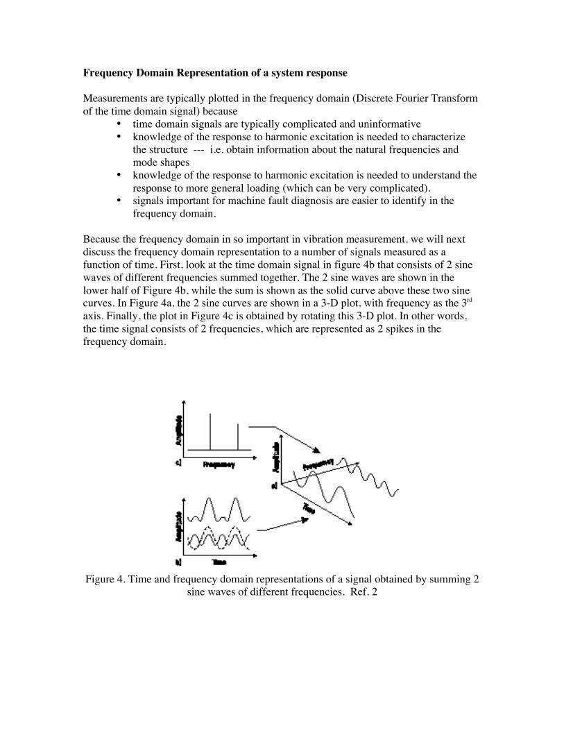
Because the frequency domain in so important in vibration measurement, we will nextdiscuss the frequency domain representation to a number of signals measured as afunction of time. First, look at the time domain signal in figure 4b that consists of 2 sinewaves of different frequencies summed together. The 2 sine waves are shown in thelower half of Figure 4b, while the sum is shown as the solid curve above these two sinecurves. In Figure 4a, the 2 sine curves are shown in a 3-D plot, with frequency as the 3rd

axis. Finally, the plot in Figure 4c is obtained by rotating this 3-D plot. In other words,the time signal consists of 2 frequencies, which are represented as 2 spikes in thefrequency domain.

Figure 4. Time and frequency domain representations of a signal obtained by summing 2sine waves of different frequencies. Ref. 2

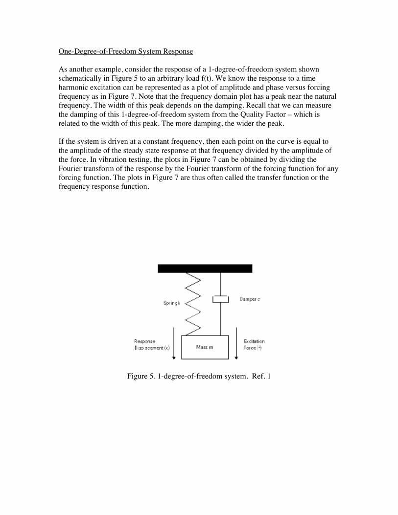
One-Degree-of-Freedom System Response

As another example, consider the response of a 1-degree-of-freedom system shownschematically in Figure 5 to an arbitrary load f(t). We know the response to a timeharmonic excitation can be represented as a plot of amplitude and phase versus forcingfrequency as in Figure 7. Note that the frequency domain plot has a peak near the naturalfrequency. The width of this peak depends on the damping. Recall that we can measurethe damping of this 1-degree-of-freedom system from the Quality Factor – which isrelated to the width of this peak. The more damping, the wider the peak.

If the system is driven at a constant frequency, then each point on the curve is equal tothe amplitude of the steady state response at that frequency divided by the amplitude ofthe force. In vibration testing, the plots in Figure 7 can be obtained by dividing theFourier transform of the response by the Fourier transform of the forcing function for anyforcing function. The plots in Figure 7 are thus often called the transfer function or thefrequency response function.

Figure 5. 1-degree-of-freedom system. Ref. 1

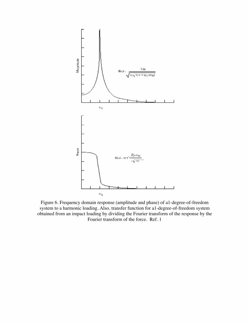
Figure 6. Frequency domain response (amplitude and phase) of a1-degree-of-freedomsystem to a harmonic loading. Also, transfer function for a1-degree-of-freedom system

obtained from an impact loading by dividing the Fourier transform of the response by theFourier transform of the force. Ref. 1

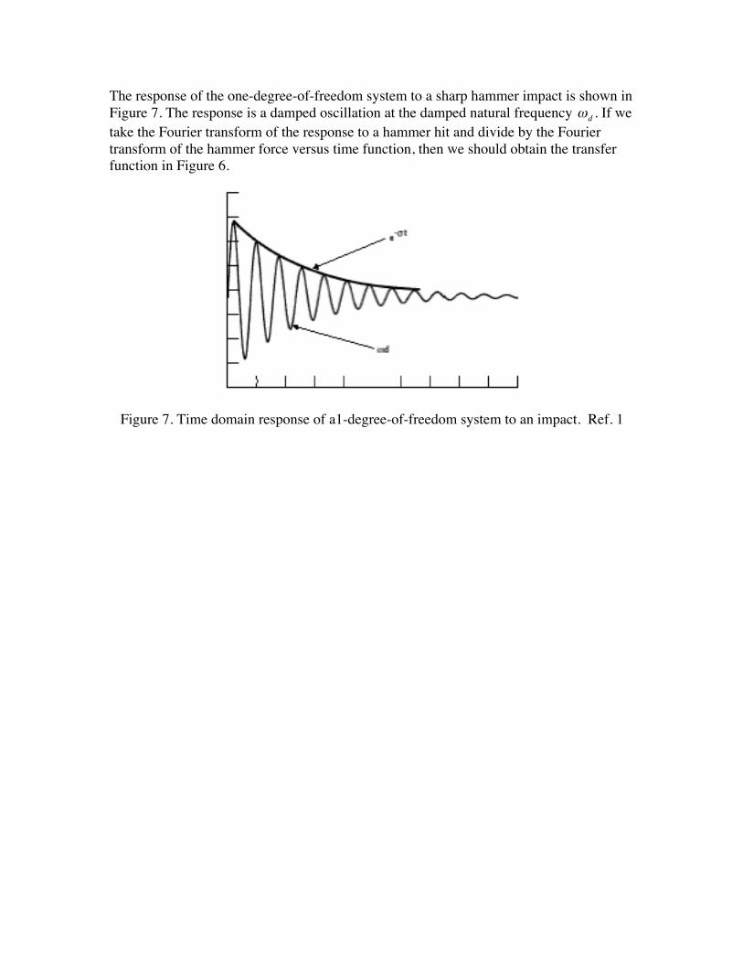
The response of the one-degree-of-freedom system to a sharp hammer impact is shown inFigure 7. The response is a damped oscillation at the damped natural frequency ωd . If wetake the Fourier transform of the response to a hammer hit and divide by the Fouriertransform of the hammer force versus time function, then we should obtain the transferfunction in Figure 6.

Figure 7. Time domain response of a1-degree-of-freedom system to an impact. Ref. 1

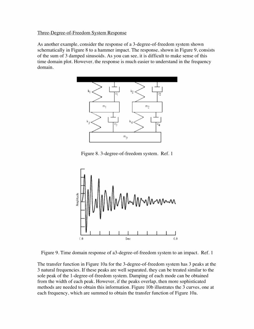
Three-Degree-of-Freedom System Response

As another example, consider the response of a 3-degree-of-freedom system shownschematically in Figure 8 to a hammer impact. The response, shown in Figure 9, consistsof the sum of 3 damped sinusoids. As you can see, it is difficult to make sense of thistime domain plot. However, the response is much easier to understand in the frequencydomain.

Figure 8. 3-degree-of-freedom system. Ref. 1

Figure 9. Time domain response of a3-degree-of-freedom system to an impact. Ref. 1

The transfer function in Figure 10a for the 3-degree-of-freedom system has 3 peaks at the3 natural frequencies. If these peaks are well separated, they can be treated similar to thesole peak of the 1-degree-of-freedom system. Damping of each mode can be obtainedfrom the width of each peak. However, if the peaks overlap, then more sophisticatedmethods are needed to obtain this information. Figure 10b illustrates the 3 curves, one ateach frequency, which are summed to obtain the transfer function of Figure 10a.

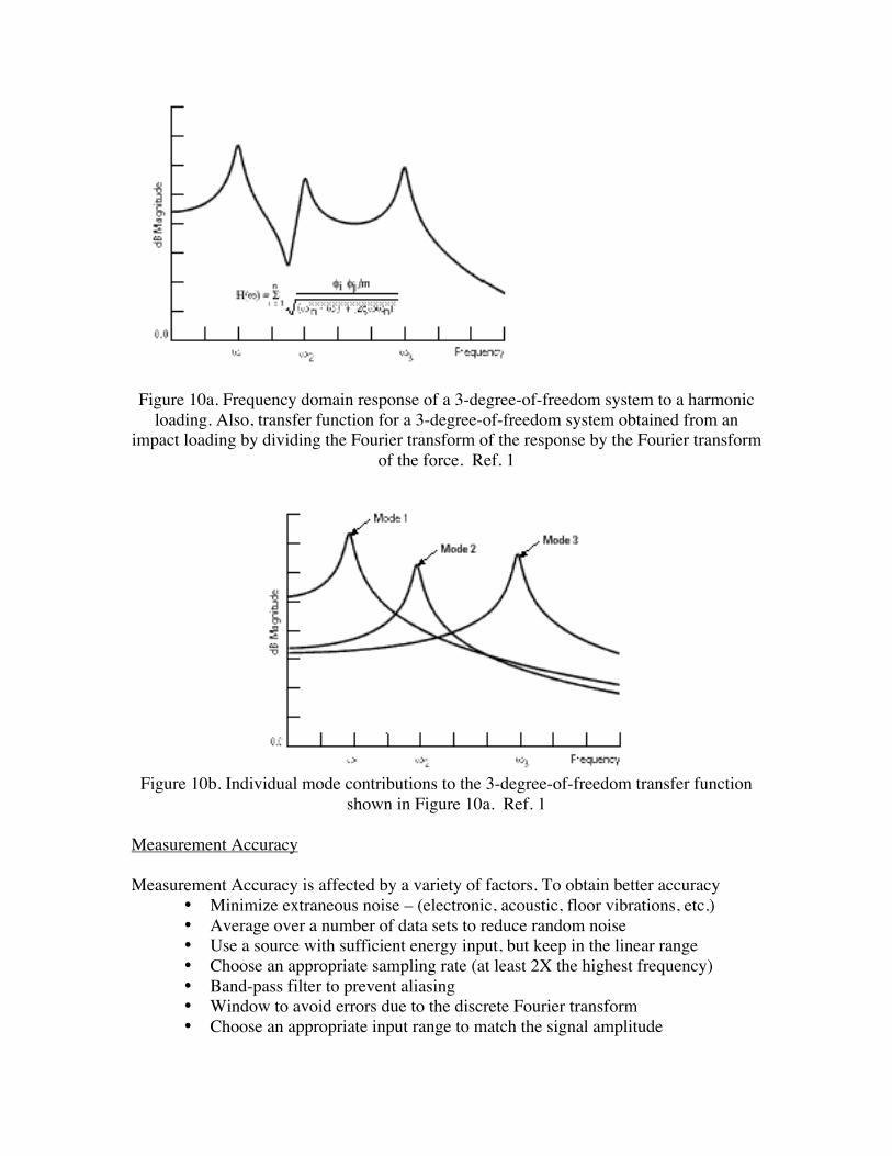
Figure 10a. Frequency domain response of a 3-degree-of-freedom system to a harmonicloading. Also, transfer function for a 3-degree-of-freedom system obtained from an

impact loading by dividing the Fourier transform of the response by the Fourier transformof the force. Ref. 1

Figure 10b. Individual mode contributions to the 3-degree-of-freedom transfer functionshown in Figure 10a. Ref. 1

Measurement Accuracy

Measurement Accuracy is affected by a variety of factors. To obtain better accuracy• Minimize extraneous noise – (electronic, acoustic, floor vibrations, etc.)• Average over a number of data sets to reduce random noise• Use a source with sufficient energy input, but keep in the linear range• Choose an appropriate sampling rate (at least 2X the highest frequency)• Band-pass filter to prevent aliasing• Window to avoid errors due to the discrete Fourier transform• Choose an appropriate input range to match the signal amplitude

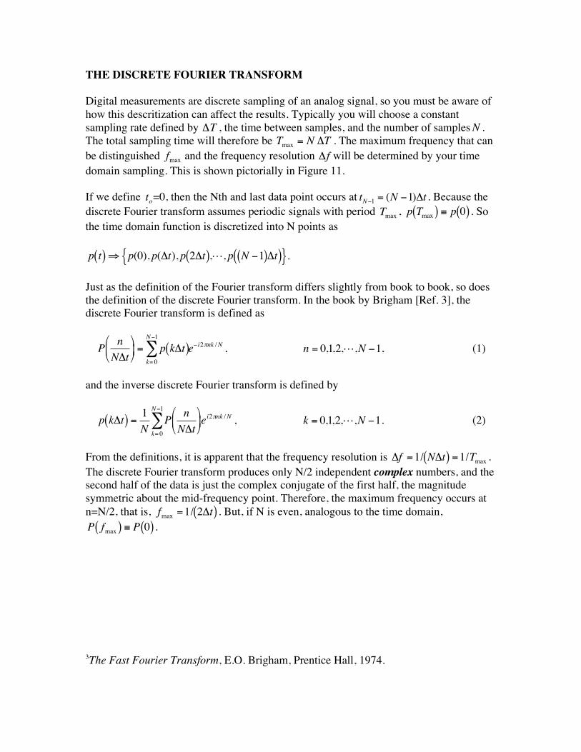
THE DISCRETE FOURIER TRANSFORM

Digital measurements are discrete sampling of an analog signal, so you must be aware ofhow this descritization can affect the results. Typically you will choose a constantsampling rate defined by ΔT , the time between samples, and the number of samplesN .The total sampling time will therefore be Tmax = N ΔT . The maximum frequency that canbe distinguished fmax and the frequency resolution Δf will be determined by your timedomain sampling. This is shown pictorially in Figure 11.

If we define

€

to=0, then the Nth and last data point occurs at

€

tN−1 = (N −1)Δt . Because thediscrete Fourier transform assumes periodic signals with period

€

Tmax ,

€

p Tmax( ) ≡ p 0( ) . Sothe time domain function is discretized into N points as

€

p t( )⇒ p(0), p(Δt), p 2Δt( ),L, p N −1( )Δt( ){ }.

Just as the definition of the Fourier transform differs slightly from book to book, so doesthe definition of the discrete Fourier transform. In the book by Brigham [Ref. 3], thediscrete Fourier transform is defined as

€

P nNΔt

= p kΔt( )

k= 0

N−1

∑ e− i2πnk /N ,

€

n = 0,1,2,L,N −1, (1)

and the inverse discrete Fourier transform is defined by

€

p kΔt( ) =1N

P nNΔt

ei2πnk /N

k= 0

N−1

∑ ,

€

k = 0,1,2,L,N −1. (2)

From the definitions, it is apparent that the frequency resolution is

€

Δf =1/ NΔt( ) =1/Tmax .The discrete Fourier transform produces only N/2 independent complex numbers, and thesecond half of the data is just the complex conjugate of the first half, the magnitudesymmetric about the mid-frequency point. Therefore, the maximum frequency occurs atn=N/2, that is,

€

fmax =1/ 2Δt( ) . But, if N is even, analogous to the time domain,

€

P fmax( ) ≡ P 0( ) .

3The Fast Fourier Transform, E.O. Brigham, Prentice Hall, 1974.

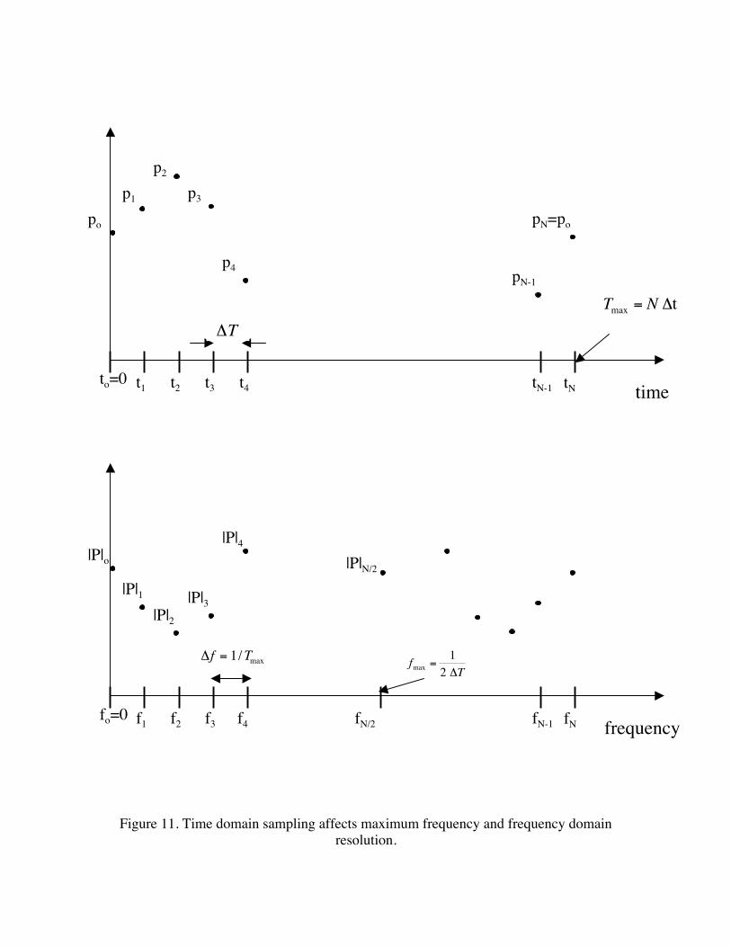
Figure 11. Time domain sampling affects maximum frequency and frequency domainresolution.

ΔT

€

Tmax = N Δt

po

p1

p2

p3

p4

to=0 t1 t3t2 t4

pN-1

pN=po

tNtN-1 time

Δf = 1/Tmax

€

fmax =1

2 ΔT

|P|o

|P|1|P|2

|P|3

|P|4

fo=0 f1 f3f2 fN/2

|P|N/2

fNfN-1 frequencyf4

Here we repeat the two important relationships between the time and frequency domainsampling.

MAXIMUM FREQUENCY SAMPLED: fmax =1

2 ΔT(3)

FREQUENCY RESOLUTION: Δf =fmax

N / 2 =

1Tmax

(4)

The first equation is a statement of the Nyquist Criterion – the sampling rate 1/ ΔT mustbe at least twice the highest frequency. That is, there must be at least 2 samples per cycleto identify the frequency correctly.

The second equation results from the restriction that there are N /2 complex data points inthe frequency domain corresponding to the N data points in the time domain. These aredemonstrated in Figure11.

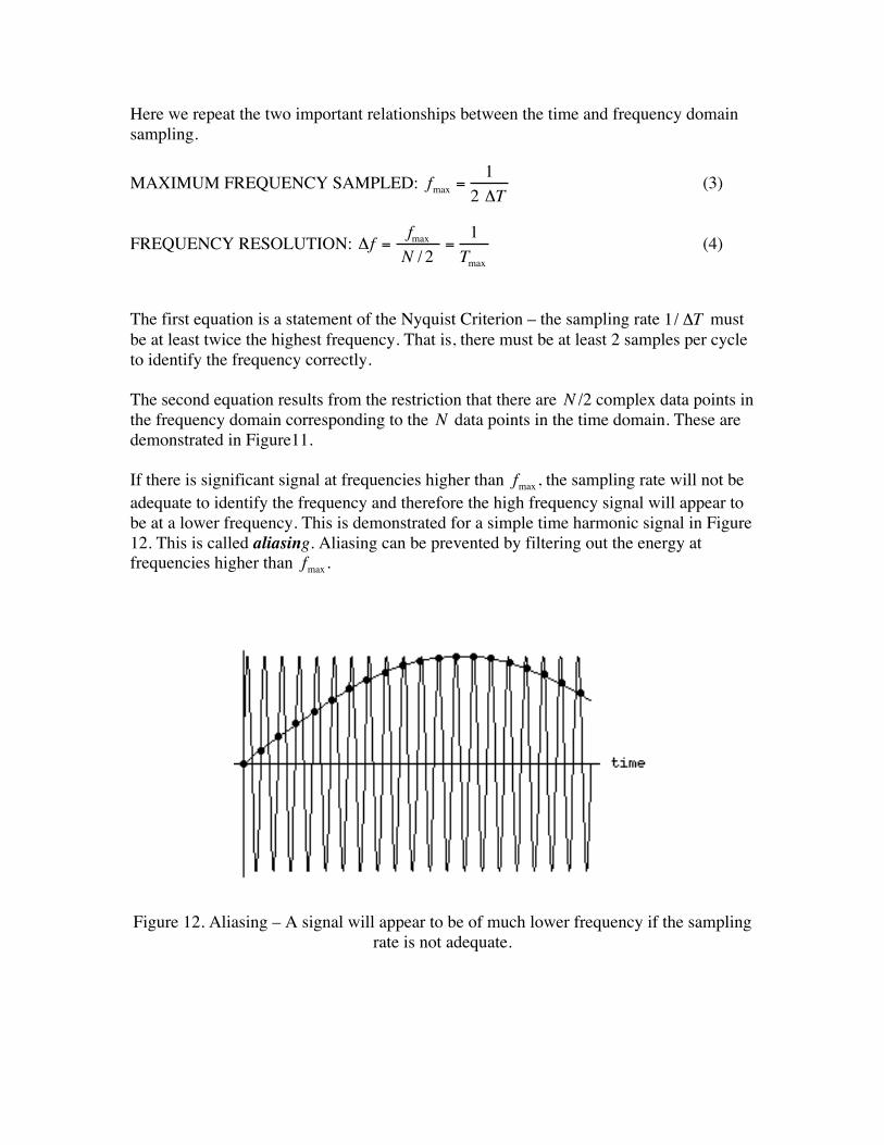
If there is significant signal at frequencies higher than fmax , the sampling rate will not beadequate to identify the frequency and therefore the high frequency signal will appear tobe at a lower frequency. This is demonstrated for a simple time harmonic signal in Figure12. This is called aliasing. Aliasing can be prevented by filtering out the energy atfrequencies higher than fmax .

Figure 12. Aliasing – A signal will appear to be of much lower frequency if the samplingrate is not adequate.

If we compare the definition of the discrete Fourier transform to that of the complexFourier series, we can then determine the amplitude of the contribution at each frequency.

The complex Fourier series of a periodic function

€

f t( )with period

€

T1 = 2π /Ω1 can bedefined as

€

f t( ) = FneinΩ1t

n=−∞

∞

∑ , where ,

€

Fn =1T1

f t( )0

T1

∫ e− inΩ1t . (5)

The energy at frequency

€

nΩ1 is equal to

€

Fn + F−n = 2Fn . So if we approximate theintegral for

€

Fn as a summation of discrete data points, then we obtain

€

Fn =1T1

f t( )0

T1

∫ e− in2πt /T1 ≈ 1NΔt

f kΔt( )e− in2π kΔt

NΔtΔt =k= 0

N−1

∑ 1N

f kΔt( )e− i2πnk /Nk= 0

N−1

∑ (6)

By comparing the definition of the Fourier series in Equation (6) to the definition used inRef. 3 for the discrete Fourier transform in Equation (2), we conclude that the discreteFourier transform amplitude

€

Pn must be multiplied by

€

2 /N to obtain the contribution atthe frequency

€

nΔf .

Mathematica uses a slightly different definition for the discrete Fourier transform pair.Let

€

bs{ } represent the list that is the DFT of the list

€

ar{ }, where

€

r,s =1,2,3,L,N . Thenthe Mathematica commands relating these two lists are

€

bs{ } = Fourier ar{ }[ ] and

€

ar{ } = InverseFourier bs{ }[ ] . (7)

Mathematica’s definitions are

€

bs =1N

are2πi r−1( ) s−1( ) /N

r=1

N

∑ and

€

ar =1N

bse−2πi r−1( ) s−1( ) /N

r=1

N

∑ . (8)

The only substantive difference between the definitions in Equations (1) and (2) and thedefinitions in Equation (8) is that the amplitude of the Mathematica’s DFT is

€

1/ Ntimes the definition in Brigham’s book. Therefore, we conclude that the discrete Fouriertransform amplitude

€

bs must be multiplied by

€

2 N /N to obtain the contribution at thefrequency

€

s−1( )Δf .

WindowingDiscrete Fourier transforms assume that the signal is periodic with time period Tmax . Ifthe signal level and slope at the end does not match the signal level and slope at thebeginning, then this effectively will introduce a jump in the signal because of theassumed periodicity of the signal. This is illustrated in Figure 12. Windowing is used toweight the signal at this artificial discontinuity so that it has less of an effect on theFourier transform. However, care must be taken when using windows because they canaffect the Fourier transforms in other ways. A “Uniform” window uses a constant unityweight factor over the entire domain, i.e., it is equivalent to no window. The Uniformwindow should be used unless there is a specific reason to window the data.

The effect of using a non-uniform windowing function on a DFT is illustrated in Figures13 and 14. First, Figure 13 a) shows the time domain signal for a harmonic wave that hasthe same value and slope at the start and end. For this signal no discontinuity isintroduced and the DFT in Figure 13 b) has nonzero values only at the fundamental andthe first 2 harmonics. On the other hand, a jump in slope is introduced when the timedomain signal in Figure 13 c) is periodically extended, so the DFT of this signal, shownin Figure 13 d) is nonzero over a large range of frequencies. This smearing of the energythroughout the frequency domains is a phenomenon known as leakage. To lessen theeffect of the introduced discontinuity, a “window” can be used to weight thecontributions from the end values less. A Hanning window is the most typical windowused and its use is shown in Figure 12 c) and d). The DFT of the time domain signal inFigure 13 c) after windowing is applied is given in Figure 14. Note that the peak issharper, but not as sharp as in Figure 13 b). Care must be used in interpreting DFT, sincethe spreading of the peak in Figure 14 is not due to damping but is due to an artifact ofthe DFT.

Figure 12. Illustration of windowing a time domain signal. Ref. 1

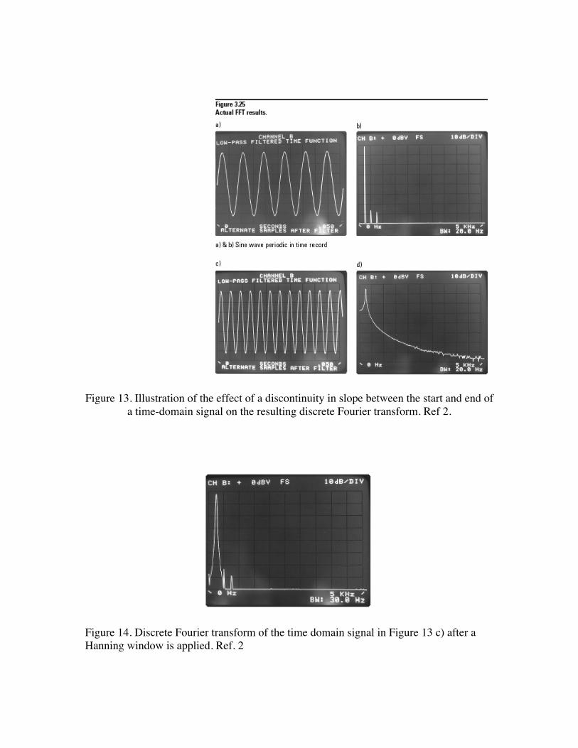
Figure 13. Illustration of the effect of a discontinuity in slope between the start and end ofa time-domain signal on the resulting discrete Fourier transform. Ref 2.

Figure 14. Discrete Fourier transform of the time domain signal in Figure 13 c) after aHanning window is applied. Ref. 2

A FlatTop windowing function works similar to a Hanning windowing function, but mayimprove the accuracy of amplitude measurements at the expensive of widening the filterrange.

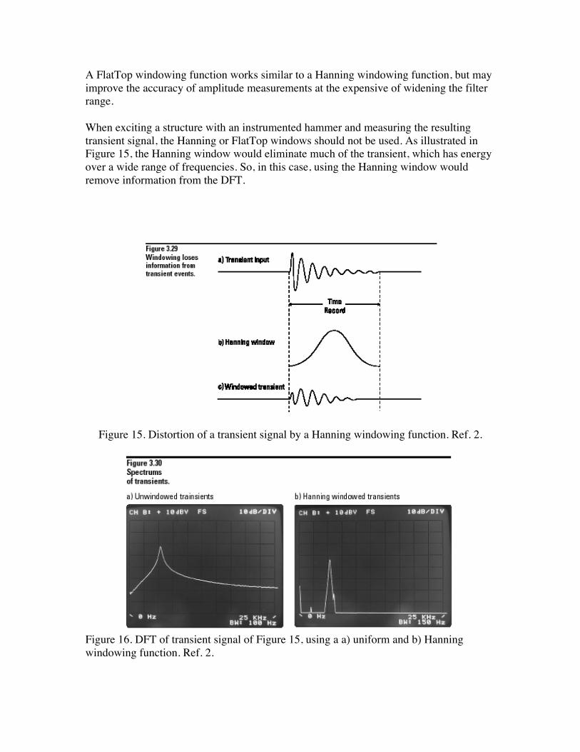
When exciting a structure with an instrumented hammer and measuring the resultingtransient signal, the Hanning or FlatTop windows should not be used. As illustrated inFigure 15, the Hanning window would eliminate much of the transient, which has energyover a wide range of frequencies. So, in this case, using the Hanning window wouldremove information from the DFT.

Figure 15. Distortion of a transient signal by a Hanning windowing function. Ref. 2.

Figure 16. DFT of transient signal of Figure 15, using a a) uniform and b) Hanningwindowing function. Ref. 2.

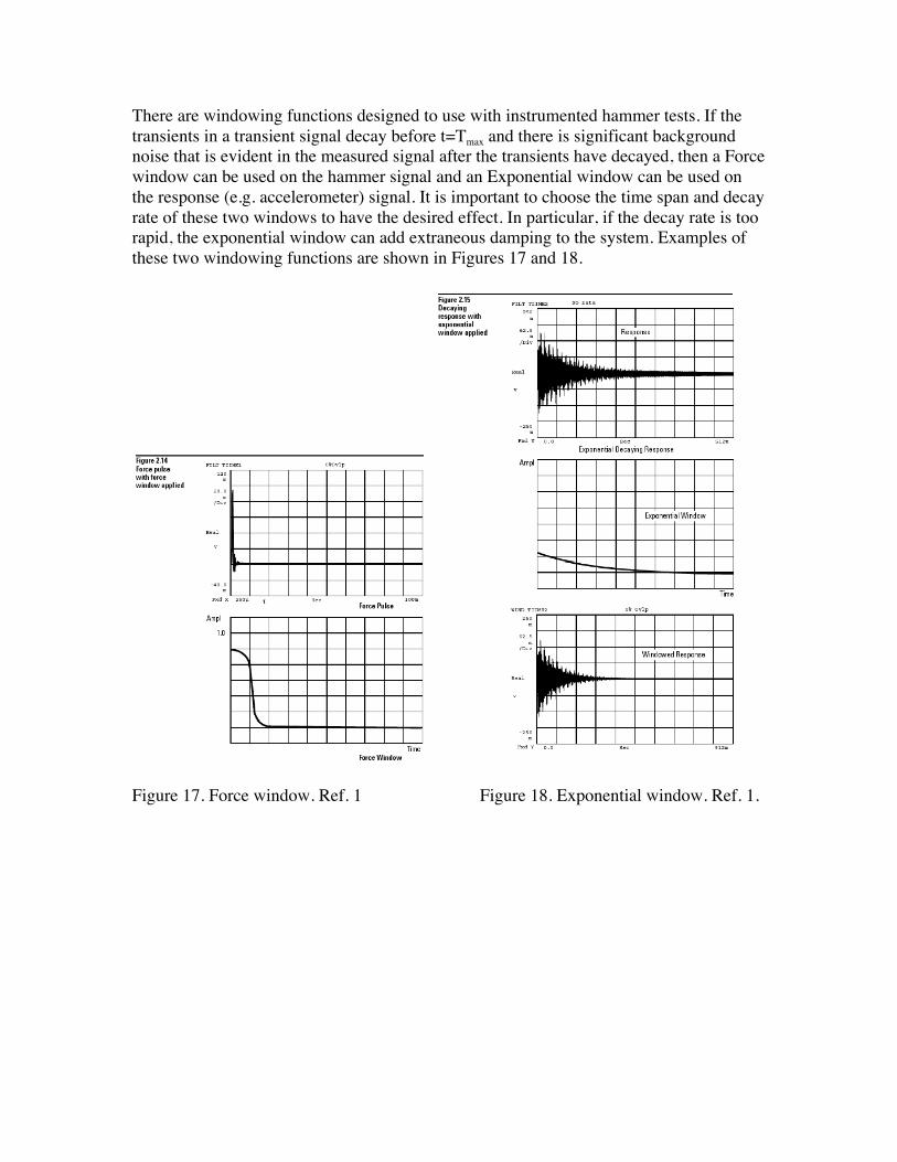
There are windowing functions designed to use with instrumented hammer tests. If thetransients in a transient signal decay before t=Tmax and there is significant backgroundnoise that is evident in the measured signal after the transients have decayed, then a Forcewindow can be used on the hammer signal and an Exponential window can be used onthe response (e.g. accelerometer) signal. It is important to choose the time span and decayrate of these two windows to have the desired effect. In particular, if the decay rate is toorapid, the exponential window can add extraneous damping to the system. Examples ofthese two windowing functions are shown in Figures 17 and 18.

Figure 17. Force window. Ref. 1 Figure 18. Exponential window. Ref. 1.

INPUT RANGE

The INPUT RANGE is also important to monitor on a digital signal analyzer. Note thatthe input range is not necessarily the display range, as is typical on an oscilloscope. If thesignal uses only a small portion of the input range, then the discritization of the signalamplitude will lead to significant error. Any part of the signal that exceeds the inputrange will not be correctly represented (this is indicated by the “overload” light). This isdemonstrated in the three sets of plots in Figure 19.

Figure 19. Illustration of the importance of using the correct input range.