
Using a LONESTARTM Portable Analyzer to Quantify the Essential Oil
Content of Spices A case study with cinnamon, ginger, cumin and cloves
Contact us
www.owlstonenanotech.com
2 of 23
Contents
Objectives........................................................................................................................................ 3
The Lonestar Platform .................................................................................................................... 4
Testing Procedure overview ........................................................................................................... 5
Determination of sample rate and sample flush ............................................................................ 5
Sample preparation for quantitative testing .................................................................................. 6
Selection of sample mass ............................................................................................................ 6
Surface area of sample ............................................................................................................... 6
Sampling vessel ........................................................................................................................... 6
Results – Cinnamon ........................................................................................................................ 7
Results – Ginger, Cumin and Cloves ............................................................................................... 9
Ginger .......................................................................................................................................... 9
Cumin ........................................................................................................................................ 10
Cloves ........................................................................................................................................ 12
Comparison of all spices ............................................................................................................... 13
Summary ....................................................................................................................................... 15
Appendix A: FAIMS Technology at a Glance ................................................................................. 16
Sample preparation and introduction ...................................................................................... 16
Carrier Gas ................................................................................................................................ 17
Ionisation Source ...................................................................................................................... 17
Mobility ..................................................................................................................................... 20
Detection and Identification ..................................................................................................... 21

3 of 23
Objectives
The aim of the testing was to demonstrate the Lonestar platforms viability for making real-time quantitative measurements of volatile oil content of cinnamon, ginger, cumin and cloves. Testing focused on the cinnamon to enable a more complete dataset to be constructed over the range of concentrations with simple viability checks on the other spices. The Lonestar method was compared to the results from the current AOAC method 932.10 (link), which uses a 5-6 hour distillation of silica-dried oils and a xylene trap to determine the percentage oil content of a 50 g sample of the spice. Secondary objectives included
Determining the typical spectra for the different spices to facilitate follow on activities to produce models which would identify any contaminations in a sample (cleaning agents, styrene etc)
Identifying the key parameters in the sampling method and the strength of the effect these parameters have to keep sampling methods as simple as possible
Devising a sample preparation method

4 of 23
The Lonestar Platform
Lonestar is a powerful and adaptable chemical monitor in a portable self contained unit. Incorporating Owlstone’s proprietary FAIMS technology (see Appendix A), the instrument offers the flexibility to provide rapid alerts and detailed sample analysis. It can be trained to respond to a broad range of chemical scenarios and can be easily integrated with other sensors and third party systems to provide a complete monitoring solution. As a result, Lonestar is suitable for a broad variety of applications ranging from process monitoring to lab based R&D.
Figure 1 Lonestar connection figures

5 of 23
Testing Procedure overview
To make gas phase measurements of the volatile oil content in spices, samples were placed in glass vials. Sample vials were connected to the Lonestar analyzer as shown in Figure 2. The headspace of a connected vial was flushed with clean air from the Lonestar at a rate fast enough to stop any build up of volatile oils in the vial headspace. This ensured that only the constant oil generation rate was measured. The aim is to build up a calibration curves of the concentration of the volatile oils versus Lonestar response for each of the spices via the measurement of this generation rate. Due to the sensitivity of the instrument most of the sample gas is flushed directly out of an attached vent with only a small proportion being drawn in by the Lonestar.
Figure 2 Connection of sample vials to the Lonestar system for headspace sampling.
Determination of sample rate and sample flush
The sample rate was selected to keep the response in range. Sample rates of approximately 10 ml min-1 were used for cinnamon samples with > 2% volatile oil (VO) content and rates of 50 ml min-1 were used for samples with < 2% VO content. This maintained the optimum signal to noise ratio whilst determining the cinnamon response curve These rates were determined by trial and error testing using cinnamon samples at the upper and lower limits of VO content (e.g. for cinnamon 1.5% and 7%)
Vent
Sample vial, with septum
Purge line
Sample line

6 of 23
It was found that sample vials needed to be flushed before the start of the measurement to remove any build up of VOs generated after the sample was loaded into the vial. A flush time of 30 seconds was found to be adequate to remove the existing VOs (The air in a 30 ml vial flushed at approximately 2 min-1 is replaced more than 30 times). This flush was not passed through the Lonestar as the initial pulse of air may have much higher concentrations of VOs being being measured and could have caused an error in the concurrent sample measurement.
Sample preparation for quantitative testing
Selection of sample mass
Initial testing showed significant generation of volatile oils from the cinnamon, it was therefore desirable to minimize the sample size to prevent saturating the Lonestar response. For the testing, 0.2 g was selected as the lowest mass which could be measured with sufficient accuracy (limited by accuracy of available balance, ±0.01 g, giving accuracy of 5%) this is the dominant error for all the testing.
Surface area of sample
As well as being related to the concentration of the oil in the spice, the rate of volatile oil generation is also affected by the surface area of the spice exposed to air. The precise strength of this dependence has yet to be quantified. In practice it is a combination of particle size and packing density of the spice which dictate the effective surface area. One of the standard sample preparations is to sieve through a 100 micron mesh then through a 50 mesh, collecting what passes through the 100 and not through the 50. This 50-100 micron preparation is used throughout the cinnamon testing.
Sampling vessel
The sample was transferred to a GC sample vial – 20 mm diameter, 15 ml volume with septum (Supelco-GLC-07501).

7 of 23
Results – Cinnamon
Testing focused on the cinnamon samples. The analytes to which the Lonestar should be most sensitive to are cinnamaldehyde, ethyl cinnamate and related esters. The relative proton affinities of the cinnamaldehyde and esters should favour cinnamaldehyde detection in most cases.
Figure 3 Species in cinnamon VO - Cinnamaldehyde (left) and Ethyl cinnamate (right).
Table 1 Test parameters
Internal flow rate 10 ml min-1
Internal humidity < 1%
Internal temperature 58°C
Sample preparation 50 mesh
Sample mass 0.2 g
Flush rate 1.9 l min-1
Figure 4 Typical cinnamon fingerprint
Three different types of cinnamon (Saigon, KA grade and KB grade) each of which have different intrinsic volatile oil content, were measured using the Lonestar. The analyte peak height at 50% DF was extracted from the measured FAIMS spectra and plotted against the VO content found using

8 of 23
AOAC distillation method 932.10 (Figure 5). This provides a calibration of the Lonestar’s response to varying VO content in cinnamon samples.
Figure 5 Cinnamon calibration curve – analyte peak height at 50% DF compared against the the volatile oil content measured measured using AOAC method 932.10.
The outlying measurement for the Saigon Cinnamon sample shows the impact of varying spice sample preparation; this stock sample was supplied for testing and showed significantly less volatile oil generation than expected. Further investigation found that the sample had been a special order that was prepared differently. The cinnamon had undergone a double grind and had been sieved through a 35 micron mesh (rather than 50 micron mesh). Finer grinding will have given the sample a larger surface area from which more VOs may have been lost prior to sampling with Lonestar.

9 of 23
Results – Ginger, Cumin and Cloves
Ginger
Two samples of ginger; one a Chinese and one Nigerian were tested. Both had measured VO content of approximately 2%. Both samples gave strong responses. However the Nigerian ginger (Figure 6) response was 25% lower than that of the Chinese ginger (Figure 7). This fits with the fact that the Nigerian sample was 5 months old (i.e. 5 months since VO measurement by AOAC method). More samples of known VO content would be required to build a calibration curve.
Figure 6 Nigerian ginger (5 months old)
Figure 7 Chinese ginger (fresh)

10 of 23
Cumin
The analyte Lonestar is most likely to detect from cumin is cuminaldehyde (Figure 8), though substituted pyrazine compounds will also be present and should contribute to the response.
Figure 8 Cuminaldehyde FAIMS spectra were collected using Lonestar for two samples of cumin were that had 1.5% and 3.5% volatile oil contents (based on AOAC distillation results).
Figure 9 Example cumin FAIMS spectra fingerprint

11 of 23
The response from the sample containing the higher VO content was significantly larger (Figure 10). More data points are required to construct a calibration curve.
Figure 10 Cumin data - higher VO content gives higher response from Lonestar

12 of 23
Cloves
Eugenol (Figure 11) makes up ~90% of the VO in cloves. Eugenol’s phenol group has the potential for negative ion formation.
Figure 11 Eugenol
Unlike the other spices measured, the cloves showed a response in the negative mode (negative ions passing through the FAIMS filter). This indicates that eugenol is the ion being detected in this case.
Figure 12 FAIMS spectra collected from a sample of cloves, note the significant negative ion response (left), likely to be from eugenol.
13 of 23
Comparison of all spices
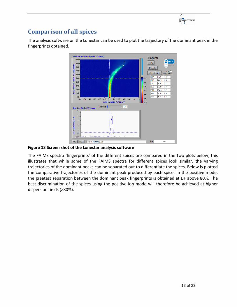
The analysis software on the Lonestar can be used to plot the trajectory of the dominant peak in the fingerprints obtained.
Figure 13 Screen shot of the Lonestar analysis software
The FAIMS spectra ‘fingerprints’ of the different spices are compared in the two plots below, this illustrates that while some of the FAIMS spectra for different spices look similar, the varying trajectories of the dominant peaks can be separated out to differentiate the spices. Below is plotted the comparative trajectories of the dominant peak produced by each spice. In the positive mode, the greatest separation between the dominant peak fingerprints is obtained at DF above 80%. The best discrimination of the spices using the positive ion mode will therefore be achieved at higher dispersion fields (>80%).

14 of 23
Figure 14 Spice dominant peak fingerprint comparison positive ion mode
Figure 15 Spice discrimination using dominant peak fingerprints including the negative mode

15 of 23
Summary
The testing showed that methods can be developed for making rapid measurements of the volatile oil content of spices by measuring the generation rate of volatile compounds into the headspace above the spice.
For cinnamon a calibration curve of volatile oil content (determined by the current AOAC method) and Lonestar response was produced showing this dependence. This shows that it is practical to use the Lonestar platform for spice volatile oil measurements.
The 5% error in weighing the spices is the limit on the method accuracy; this corresponds to +/-0.15% on a 3% VO content which is already comparable to the accuracy of the current method.
Sampling times are 2-3 minutes plus a 30 second flush before hand to stabilise the headspace (remove any volatile build up). This could be reduced significantly as only one part of the fingerprint is needed to obtain the VO content (with averaged repeat measurements 10 seconds of sampling would be sufficient). However extended sampling does enable monitoring of contaminations.
FAIMS spectra fingerprints for the different spices have been produced and the Lonestar could be trained to identify variation from the expected fingerprint to enable a simple alarm on spice contamination (e.g. by a cleaning agent, styrene etc).
A basic sample preparation has been determined. The selected weight, spice particle size and headspace volume are viable for cinnamon and provide initial starting parameters for developing methods for other spices.
16 of 23
Appendix A: FAIMS Technology at a Glance
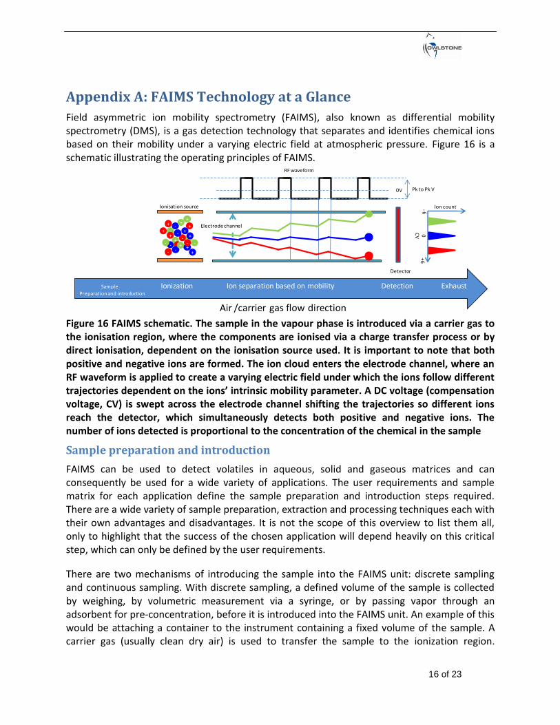
Field asymmetric ion mobility spectrometry (FAIMS), also known as differential mobility spectrometry (DMS), is a gas detection technology that separates and identifies chemical ions based on their mobility under a varying electric field at atmospheric pressure. Figure 16 is a schematic illustrating the operating principles of FAIMS.
Figure 16 FAIMS schematic. The sample in the vapour phase is introduced via a carrier gas to the ionisation region, where the components are ionised via a charge transfer process or by direct ionisation, dependent on the ionisation source used. It is important to note that both positive and negative ions are formed. The ion cloud enters the electrode channel, where an RF waveform is applied to create a varying electric field under which the ions follow different trajectories dependent on the ions’ intrinsic mobility parameter. A DC voltage (compensation voltage, CV) is swept across the electrode channel shifting the trajectories so different ions reach the detector, which simultaneously detects both positive and negative ions. The number of ions detected is proportional to the concentration of the chemical in the sample
Sample preparation and introduction
FAIMS can be used to detect volatiles in aqueous, solid and gaseous matrices and can consequently be used for a wide variety of applications. The user requirements and sample matrix for each application define the sample preparation and introduction steps required. There are a wide variety of sample preparation, extraction and processing techniques each with their own advantages and disadvantages. It is not the scope of this overview to list them all, only to highlight that the success of the chosen application will depend heavily on this critical step, which can only be defined by the user requirements.
There are two mechanisms of introducing the sample into the FAIMS unit: discrete sampling and continuous sampling. With discrete sampling, a defined volume of the sample is collected by weighing, by volumetric measurement via a syringe, or by passing vapor through an adsorbent for pre-concentration, before it is introduced into the FAIMS unit. An example of this would be attaching a container to the instrument containing a fixed volume of the sample. A carrier gas (usually clean dry air) is used to transfer the sample to the ionization region.
-6+
60
Ionisation source
-
-
+
+
+ -
+ +
-
-
-
+
-
-
+
+
+ -
++
-
--
+
CV
Detector
Electrode channel
RF waveform
Air /carrier gas flow direction
Pk to Pk V 0V
Sample Ionization Ion separation based on mobility Detection ExhaustPreparation and introduction
Ion count

17 of 23
Continuous sampling is where the resultant gaseous sample is continuously purged into the FAIMS unit and either is diluted by the carrier gas or acts as the carrier gas itself. For example, continuously drawing air from the top of a process vat.
The one key requirement for all the sample preparation and introduction techniques is the ability to reproducibly generate and introduce a headspace (vapour) concentration of the target analytes that exceeds the lower limits of detection of the FAIMS device.
Carrier Gas
The requirement for a flow of air through the system is twofold: Firstly to drive the ions through the electrode channel to the detector plate and secondly, to initiate the ionization process necessary for detection. As exhibited in Figure 17, the transmission factor (proportion of ions that make it to the detector) increases with increasing flow. The higher the transmission factor, the higher the sensitivity. Higher flow gives a larger full width half maximum (FWHM) of the peaks but also decreases the resolution of the FAIMS unit (see Figure 18). The air/carrier gas determines the baseline reading of the instrument. Therefore, for optimal operation it is desirable for the carrier to be free of all impurities (< 0.1 ppm methane) and the humidity to be kept constant. It can be supplied either from a pump or compressor, allowing for negative and positive pressure operating modes.
Ionisation Source
There are three main vapor phase ion sources in use for atmospheric pressure ionization; radioactive nickel-63 (Ni-63), corona discharge (CD) and ultra-violet radiation (UV). A comparison of ionization sources is presented in Table 2.
Ionisation Source Mechanism Chemical Selectivity
Ni63
(beta emitter) creates a positive / negative RIP Charge transfer Proton / electron affinity
UV (Photons) Direct ionisation First ionisation potential
Corona discharge (plasma) creates a positive / negative RIP
Charge transfer Proton / electron affinity
Table 2 FAIMS ionization source comparison
Figure 17 Flow rate vs. ion transmission factor
Figure 18 FWHM of ion species at set CV

18 of 23
Ni-63 undergoes beta decay, generating energetic electrons, whereas CD ionization strips electrons from the surface of a metallic structure under the influence of a strong electric field. The generated electrons from the metallic surface or Ni-63 interact with the carrier gas (air) to form stable +ve and -ve intermediate ions which give rise to reactive ion peaks (RIP) in the positive and negative FAIMS spectra (Figure 19). These RIP ions then transfer their charge to neutral molecules through collisions. For this reason, both Ni-63 and CD are referred to as indirect ionization methods.
For the positive ion formation:
N2 + e- → N2+ + e- (primary) + e- (secondary)
N2+ + 2N2 → N4
+ + N2 N4+ + H2O → 2N2 + H2O+ H2O+ + H2O → H3O+ + OH H3O+ + H2O + N2 ↔ H+(H2O)2 + N2 H+(H2O)2 + H2O + N2 ↔ H+(H2O)3 + N2
For the negative ion formation:
O2 + e- → O2-
B + H2O + O2- ↔ O2
-(H2O) + B B + H2O + O2
-(H2O) ↔ O2-(H2O)2 + B
The water based clusters (hydronium ions) in the positive mode (blue) and hydrated oxygen ions in the negative mode (red), are stable ions which form the RIPs. When an analyte (M) enters the RIP ion cloud, it can replace one or dependent on the analyte, two water molecules to form a monomer ion or dimer ion respectively, reducing the number of ions present in the RIP.
H+(H2O)3 + M + N2 ↔ MH+(H2O)2 + N2 + H2O ↔ M2H
+(H2O)1 + N2 + H2O
Dimer ion formation is dependent on the analyte’s affinity to charge and its concentration. This is illustrated in Figure 19A using dimethyl methylphsphonate (DMMP). Plot A shows that the RIP decreases with an increase in DMMP concentration as more of the charge is transferred over to the DMMP. In addition the monomer ion decreases as dimer formation becomes more favourable at the higher concentrations. This is shown more clearly in Figure 19B, which plots the peak ion current of both the monomer and dimer at different concentration levels.
Monomer Dimer

19 of 23
Figure 19 DMMP Monomer and dimer formation at different concentrations
The likelihood of ionization is governed by the analyte’s affinity towards protons and electrons (Table 3 and Table 4 respectively).
In complex mixtures where more than one chemical is present, competition for the available charge occurs, resulting in preferential ionisation of the compounds within the sample. Thus the chemicals with high proton or electron affinities will ionize more readily than those with a low proton or electron affinity. Therefore the concentration of water within the ionization region will have a direct effect on certain analytes whose proton / electron affinities are lower.
Chemical Family Example Proton affinity
Aromatic amines Pyridine 930 kJ/mole
Amines Methyl amine 899 kJ/mole
Phosphorous Compounds TEP 891 kJ/mole
Sulfoxides DMS 884 kJ/mole
Ketones 2- pentanone 832 kJ/mole
Esters Methly Acetate 822 kJ/mole
Alkenes 1-Hexene 805 kJ/mole
Alcohols Butanol 789 kJ/mole
Aromatics Benzene 750 kJ/mole
Water 691 kJ/mole
Alkanes Methane 544 kJ/mole
Table 3 Overview of the proton affinity of different chemical families
RIP
Monomer
Dimer

20 of 23
Chemical Family Electron affinity
Nitrogen Dioxide 3.91eV
Chlorine 3.61eV
Organomercurials
Pesticides
Nitro compounds
Halogenated compounds
Oxygen 0.45eV
Aliphatic alcohols
Ketones
Table 4 Relative electron affinities of several families of compounds
The UV ionization source is a direct ionization method whereby photons are emitted at energies of 9.6, 10.2, 10.6, 11.2, and 11.8 eV and can only ionize chemical species with a first ionization potential of less than the emitted energy. Important points to note are that there is no positive mode RIP present when using a UV ionization source and also that UV ionization is very selective towards certain compounds.
Mobility
Ions in air under an electric field will move at a constant velocity proportional to the electric field. The proportionality constant is referred to as mobility. As shown in Figure 20, when the ions enter the electrode channel, the applied RF voltages create oscillating regions of high (+VHF) and low (-VHF) electric fields as the ions move through the channel. The difference in the ion’s mobility at the high and low electric field regimes dictates the ion’s trajectory through the channel. This phenomenon is known as differential mobility.
Figure 20 Schematic of a FAIMS channel showing the difference in ion trajectories caused by the different mobilities they experience at high and low electric fields
Figure 21 Schematic of the ideal RF waveform, showing the duty cycle and peak to peak voltage (Pk to Pk V)
The physical parameters of a chemical ion that affect its differential mobility are its collisional cross section and its ability to form clusters within the high/low regions. The environmental factors within the electrode channel affecting the ion’s differential mobility are electric field, humidity, temperature and gas density (i.e. pressure).
-VLF
+VHF
Difference in mobility
Pk to Pk V 0V
+VHF
-VLF d
Duty Cycle = d/t t

21 of 23
The electric field in the high/low regions is supplied by the applied RF voltage waveform (Figure 21). The duty cycle is the proportion of time spent within each region per cycle. Increasing the peak-to-peak voltage increases/decreases the electric field experienced in the high/low field regions and therefore influences the velocity of the ion accordingly. It is this parameter that has the greatest influence on the differential mobility exhibited by the ion.
It has been shown that humidity has a direct effect on the differential mobility of certain chemicals, by increasing/decreasing the collision cross section of the ion within the respective low/high field regions. The addition and subtraction of water molecules to analyte ions is referred to as clustering and de-clustering. Increased humidity also increases the number of water molecules involved in a cluster (MH+(H2O)2) formed in the ionisation region. When this cluster experiences the high field in between the electrodes the water molecules are forced away from the cluster reducing the size (MH+) (de-clustering). As the low field regime returns so do the water molecules to the cluster, thus increasing the ion’s size (clustering) and giving the ion a larger differential mobility. Gas density and temperature can also affect the ion’s mobility by changing the number of ion-molecule collisions and changing the stability of the clusters, influencing the amount of clustering and de-clustering.
Changes in the electrode channel’s environmental parameters will change the mobility exhibited by the ions. Therefore it is advantageous to keep the gas density, temperature and humidity constant when building detection algorithms based on an ion’s mobility as these factors would need to be corrected for. However, it should be kept in mind that these parameters can also be optimized to gain greater resolution of the target analyte from the background matrix, during the method development process.
Detection and Identification
As ions with different mobilities travel down the electrode channel, some will have trajectories that will result in ion annihilation against the electrodes, whereas others will pass through to hit the detector. To filter the ions of different mobilities onto the detector plate a compensation voltage (CV) is scanned between the top and bottom electrode (see Figure 22). This process realigns the trajectories of the ions to hit the detector and enables a CV spectrum to be produced. The ion’s mobility is thus expressed as a compensation voltage at a set electric field. Figure 23 shows an example CV spectrum of a complex sample where a de-convolution technique has been employed to characterize each of the compounds.
Figure 22 Schematic of the ion trajectories at different compensation voltages and the resultant FAIMS spectrum
CV -6V
Detector
CV 6V
-6
V+6V
-0V
CV -6V
Detector
CV 6V
-6
V+6
V-
0V
CV-6V
Detector
CV 6V
-6V+6
V-0V
CV = -5V
CV = 0V
CV = 5V

22 of 23
Changing the applied RF peak-to-peak voltage (electric field) has a proportional effect on the ion’s mobility. If this is increased after each CV spectrum, a dispersion field matrix is constructed. Figure 24 shows two examples of how this is represented; both are negative mode dispersion field (DF) sweeps of the same chemical. The term DF is sometimes used instead of electric field. It is expressed as a percentage of the maximum peak-to-peak voltage used on the RF waveform. The plot on the left is a waterfall image where each individual CV scan is represented by compensation voltage (x-axis), ion current (y-axis) and electric field (z-axis). The plot on the right is the one that is more frequently used and is referred to as a 2D color plot. The compensation voltage and electric field are on the x, and y axes and the ion current is
represented by the color contours.
Figure 24 Two different examples of FAIMS dispersion field matrices with the same reactive ion peaks (RIP) and product ion peaks (PIP). In the waterfall plot on the left, the z axis is the ion current; this is replaced in the right, more frequently used, colorplot by color contours
With these data rich DF matrices a chemical fingerprint is formed, in which identification parameters for different chemical species can be extracted, processed and stored. Figure 25 shows one example: here the CV value at the peak maximum at each of the different electric field settings has been extracted and plotted, to be later used as a reference to identify the same chemicals. In Figure 26 a new sample spectrum has been compared to the reference spectrum and clear differences in both spectra can be seen.
PIPRIP
Figure 23 Example CV spectra. Six different chemical species with different mobilities are filtered through the electrode channel by scanning the CV value
Electric Field
Compensation voltage
PIP
RIP
P1
P2
P3
P4 P5
P6

23 of 23
Figure 25 On the left are examples of positive (blue) and negative (red) mode DF matrices recorded at the same time while a sample was introduced into the FAIMS detector. The sample contained 5 chemical species, which showed as two positive product ion peaks (PPIP) and three negative product ion peaks (NPIP). On the right, the CV at the PIP’s peak maximum is plotted against % dispersion field to be stored as a spectral reference for subsequent samples.
Figure 26 Comparison of two new DF plots with the reference from Figure 10. It can be seen that in both positive and negative modes there are differences between the reference product ion peaks and the new samples
0
10
20
30
40
50
60
70
80
90
100
-0.5 0 0.5 1 1.5 2 2.5
CV / V
DF
/ % Pork at 7 Days
0
10
20
30
40
50
60
70
80
90
-1.5 -1 -0.5 0 0.5 1 1.5
CV / V
DF
/ % Pork at 7 Days
PPIP 1
PPIP 2
NPIP 1
NPIP 2
NPIP 3
PPIP 1
PPIP 2
NPIP 1
NPIP 2
NPIP 3


