Download - UK Climate Projections science report: Projections …cedadocs.ceda.ac.uk/1335/1/weather_generator_full_report.pdfUK Climate Projections science report: Projections of future daily

UK Climate Projections science report: Projections of future daily climate for the UK from the Weather Generator

Phil Jones, Colin Harpham, Climatic Research Unit, School of Environmental Sciences, University of East Anglia, Chris Kilsby, Vassilis Glenis, Aidan Burton, School of Civil Engineering and Geosciences, Newcastle University

Revised November 2010

CLIMATEPROJECTIONSUK

Acknowledgements

National review group

Dr Paul Bowyer, UK Climate Impacts Programme, Oxford Anna Steynor, UK Climate Impacts Programme, Oxford Roger Street, UK Climate Impacts Programme, Oxford Dr Rachel Capon, ARUP, London Dr Vic Crisp, CIBSE (Chartered Institution of Building Services Engineers), London Karl Hardy, Flood Management, Defra, London Kathryn Humphrey, Adapting to Climate Change, Defra, London Dr Jenny Maresh, Adapting to Climate Change, Defra, London Dr Geoff Jenkins, Met Office Hadley Centre, Exeter Prof. John Mitchell, Met Office Hadley Centre, Exeter Ag Stephens, British Atmospheric Data Centre (BADC), Exeter Dr Steven Wade, HR Wallingford, Wallingford, Oxfordshire Prof. Rob Wilby, Loughborough University, Loughborough

International review group

Dr Elaine Barrow, Climate Consultant, Regina, Canada Dr Tim Carter, Finnish Environment Centre, Helsinki Prof. Alberto Montanari, University of Bologna

Reviewers’ comments have been extremely valuable in improving the final draft of this report. However, not all changes requested by all reviewers have been accepted by the authors, and the final report remains the responsibility of the authors.

3

Contents

1 The UK Climate Projections Weather Generator and how it works 7

1.1 Need for a Weather Generator 71.2 Principles of Weather Generators (WGs) 71.3 How the Weather Generator works 8

2 Using the Weather Generator to produce extremes 14

3 Proving the perturbation of the Weather Generator 17 for future periods works

4 Projections of change 24

4.1 Projected changes for sites 244.2 Projected patterns of change from the Weather Generator 27

5 Limitations of the Weather Generator 29

5.1 Lack of physical basis 295.2 The WG and the RCM grid resolution (5 km versus 25 km) 305.3 Point vs spatial data 305.4 Hourly data 315.5 Extreme events 315.6 Long term variability 32

6 References 34

Annex: Further details about the Weather Generator 35

1 Rainfall model 352 Generating the other variables 363 Further validation 384 Discussion of perturbation methodology 385 Hourly weather 406 Threshold Detector 417 Further discussion of limitations 43References 44

5


The UK Climate Projections (UKCP09) uses a Weather Generator

tool to create synthetic time series of weather variables at 5 km

resolution, which are consistent with the underlying climate

projections.

In this report we introduce the UKCP09 Weather Generator (WG). Section 1 outlines the needs and principles, while Section 2 addresses how it can be used to assess changes in extremes at spatial and temporal scales finer than the UKCP09 probability distribution functions (PDFs) can provide. Section 3 provides an illustration that the way the WG is perturbed to account for future climate change works. Section 4 provides some illustrative maps of changes in extremes across the UK and also of some key extreme metrics at some selected locations.

There are numerous discussion issues related to the use of the WG in the climate change context: the nature of the data generated by the WG is outlined in The Nature of the Weather Generator, below, and the issues are brought together in the final section on the limitations of the WG (Section 5). The principal aim of the WG is to provide users with sufficient spatial and temporal detail for their needs, detail that can be justified in the context of the PDFs. Previous UK Climate Impacts Programme (UKCIP) climate change scenarios (e.g. UKCIP02) provided much necessary detail, but many users subsequently applied a variety of downscaling procedures each tailored to their needs, which has caused inconsistency and confusion across and within the numerous impact sectors. For UKCP09, the use of a WG will provide the means for the provision of a consistent set of downscaled information (dependent on the PDF choices) across sectors and across the UK. The detail given in this report is for the general reader. Necessary, but less important additional detail is given in the Annex.

The three Science Reports, and the methodologies used to generate the UKCP09 projections, have been reviewed, firstly by the project Steering Group and User Panel, and secondly by a smaller international panel of experts. Reviewers’ comments have been taken into account in improving the reports.

The nature of the Weather Generator

The WG provides time series of weather variables which quantify some (but not all) aspects of weather on a daily or hourly basis. These variables are temperature,

Projections of future daily climate for the UK from the Weather Generator

6

rainfall, humidity and sunshine amount. The WG does not provide information on other aspects of weather such as wind, thunder/lightning and atmospheric pressure. Also, because the outputs are generated for single sites, they cannot be used to generate weather maps for the whole country at the same time.

An often used definition of climate is the average of the weather. In the same way, the average (and other statistical properties, such as maximum and minimum values) of the WG outputs can be modified to correspond with future climates projected by climate models. This does not mean that the WG outputs are associated with specific real days (e.g. a historical date, or a forecast for a real date in the future). Rather, they are just statistically credible representations of what may occur, with statistical properties (or climate) resembling those of real observed weather variables (for present day conditions) and for the future when combined with the climate signal in the UK Climate Projections.

7


1.1 Need for a Weather Generator

Impact and adaptation assessments of climate change often require more detailed information than is available from the UKCP09 PDFs described in the UK Climate Projections science report: Climate change projections (Murphy et al. 2009). Extra detail may be needed in terms of higher resolution in space and/or time. For example, projections may be needed at a specific location (a town or small river catchment) rather than an average for a 25 by 25 km grid box, or the intensity of rainfall may be needed on a time scale of an hour or day, rather than the monthly or seasonal value or the long-term average. This type of information may be further analysed in terms of exceedances of thresholds, or accumulations/deficits: these cannot be derived from the UKCP09 probabilistic projections directly. As well as more resolution, some impact assessments are carried out using models which require time series inputs, as they are simulating processes which are sensitive to the history or sequence of events, rather than simply an aggregated average. Examples of such impact models are to be found in numerous applications such as agricultural and ecological studies, or water resource and flood risk assessments.

To be useful, these generated series must be internally consistent between weather variables (e.g. so that temperatures are usually higher on dry days, compared to wet days in the summer). Such data are also needed for both the current climate and a range of possible future periods chosen by the user, so they must also be consistent with a range of observed and projected statistics of the variables (from the UKCP09 probabilistic projections). A further desirable property is that they should adequately represent extreme events such as prolonged rainfall, droughts and heatwaves.

Such high spatial and temporal resolution series are not available from the UK Climate Projections (or indeed from any other climate modelling programme), so a complementary approach has been developed in UKCP09 using a weather generator to provide high resolution time series of weather variables at a 5 by 5 km grid square resolution for user-specified future periods.

1.2 Principles of Weather Generators (WGs)

The methodology uses stochastic models to generate synthetic time series of weather variables. These weather series may be thought of as sequences that closely mimic the characteristics of real weather that could happen but have not or almost certainly will not actually be observed. A stochastic process (sometimes

1 The UK Climate Projections Weather Generator and how it works

8

Projections of future daily climate for the UK from the Weather Generator — Chapter 1

known as a random process) is one where the state of the system at one time (e.g. the weather today) does not completely determine the state at the next time (e.g. tomorrow’s weather). This is in contrast to a deterministic process, which like a weather forecast relies on such dependencies. The accuracy of a deterministic numerical weather forecast deteriorates beyond a few days into the future, so forecasts have to be renewed by re-specifying the initial conditions every few hours based on the latest weather observations. In a Weather Generator, the simulation period may be over many decades, so deterministic forecasting is not appropriate. However, the weather is not completely random either — the weather on a particular day is related to that on the previous day and there are also dependencies between weather variables, both of which can be described statistically. For instance, the temperature on day 2 is related both to the temperature on day 1 and to whether or not day 2 is wet or dry.

A WG allows us to generate many different (but statistically equivalent) series. Such generated series will be stationary, a very useful statistical property. Stationarity means that they will contain realistic day-to-day and year-to-year weather variability, but there will be little variation in the statistical description of that variability over the long term (i.e. the climate). We can also use such very long series (e.g. at least 1000 yr) for studies of extremes when observed series are not long enough, or are subject to some change over time. It is, however, recognised that there will be long-term changes in the real climate, but in the context of the UKCP09 projections, stationarity can be assumed for each user-defined future 30-year time period. Combining generated series from two different future time periods will violate this property.

Stochastic models and Weather Generators have been used for many years in fields such as flood risk estimation and water resources engineering, in a process known as Monte Carlo simulation. This allows many different eventualities and designs to be evaluated (often for specific future time horizons), and they form the basis for much of modern risk management. Such approaches are particularly appropriate for use with the probabilistic information supplied by UKCP09.

1.3 How the Weather Generator works

The UKCP09 Weather Generator is based around a stochastic rainfall model that simulates future rainfall sequences. Other weather variables are then generated according to the rainfall state. Statistical measures within the Weather Generator are then modified according to the probabilistic projections developed in UKCP09.

Weather generators mostly work in the same way, with rainfall generally taken to be the primary variable (Wilks and Wilby, 1999), so that depending on whether the day is wet or dry, other weather variables (in the UKCP09 WG these are: mean daily temperature, diurnal temperature range, vapour pressure and sunshine) are determined by mathematical/statistical relationships with rainfall and values of the variables on the previous day. These inter-variable relationships (or IVRs) maintain both the consistency between and within each of the variables.

9


The general approach taken in the UKCP09 WG is as follows:

• observed daily rainfall totals and values of other weather variables for a baseline climate (1961–1990 for rainfall and 1961–1995 for the other variables) are used to calibrate the WG (i.e. the calculation of the necessary averages, standard deviations and IVRs);

• Change Factors at the monthly time scale for each grid square are taken from the UKCP09 probabilistic projections to define the range of possible climate change futures;

• the stochastic rainfall model is then refitted using perturbed future daily rainfall statistics;

• other weather variables are then generated conditioned on the rainfall series (occurrence and amount), additionally perturbed using the Change Factors but with the observationally-based IVRs.

The fitting process is described in detail in the Annex. In the fitting of the WG, numerous parameters are estimated from statistical measures. At least 30 yr of data are required to fit the WG. For rainfall (for which gridded data are available) the period 1961–1990 was selected. For the other variables, we were only able to use station data, so used a longer period (1961–1995) to allow for a small fraction of missing data in some series. Data availability reduces if more recent years are included. In order that temperature averages given in the WG agree with 1961–1990 averages, WG output is adjusted to conform to this average (for details see the Annex).

The Change Factors used are a set of changes for all WG variables (defined by the UKCP09 probabilistic projections) for the specified future compared to the modelled baseline climate. The set involves changes in the averages of the climate variables and some additional statistical properties for rainfall and temperature (see the rest of this Report and the Annex). An example of the Change Factors is given in Section 3.

The success of the procedure in producing realistic weather sequences therefore depends to a large extent on the method of rainfall generation (Hutchinson, 1986). The well-known WG developed by Richardson (1981) incorporates the simplest method, a first-order Markov chain model. However, it is now widely recognised (Srikanthan and McMahon, 2001) that the clustered nature of rainfall occurrence is better modelled by more complex clustered point process rainfall models. So, in the UKCP09 WG one of these, the Neyman-Scott Rectangular Processes (NSRP) model is used. The NSRP model is the basis for standard UK urban drainage design software (Cowpertwait et al. 1996). This model has been shown to realistically reproduce extreme values for engineering impact studies, using multi-site data of intense events (Cowpertwait et al. 2002) and for single-site data under present and future climates (Kilsby et al. 2007). The NSRP model is described in more detail in the Annex.

In general, the parameters of the NSRP model can be estimated by selecting a set that matches, as closely as possible, the expected statistics of the generated time series with the corresponding statistics estimated from an observed rainfall time series. These statistics are derived in the first instance from observed rainfall and include: mean, variance, skewness and autocorrelation of daily rainfall amounts, and the proportion of dry days.

10


Once the precipitation sequence has been generated, other weather variables can be generated, maintaining the observed relationships between the variables. These relationships are collectively referred to as IVRs (see the Annex for details of the procedure and form of these relationships). Each of the other WG variables is normalized by subtracting the appropriate mean and dividing by the daily standard deviation for each half month of the year (used to better approximate the annual cycle of the non-rainfall variables); there being five different distributions or transitions, determined by the wet/dry status of the preceding and the current day, i.e. wet-wet, dry-dry, wet-dry, dry-wet and dry-dry-dry. The WG then generates time series for the following four variables:

• Daily mean temperature T• Daily temperature range R• Vapour pressure VP• Sunshine duration S

From these variables we calculate potential evapotranspiration (PET) using the FAO-modified (Food and Agriculture Organization of the United Nations) version of the Penman method (described in Ekström et al. 2007). The values of mean daily temperature (T) and the diurnal temperature range (R) can then be used to calculate maximum and minimum temperatures. Relative humidity is also calculated from vapour pressure using the saturation vapour pressure at the mean temperature. Direct and diffuse radiation are additionally calculated from formulae given by Muneer (2004), based principally on the daily sunshine amounts.

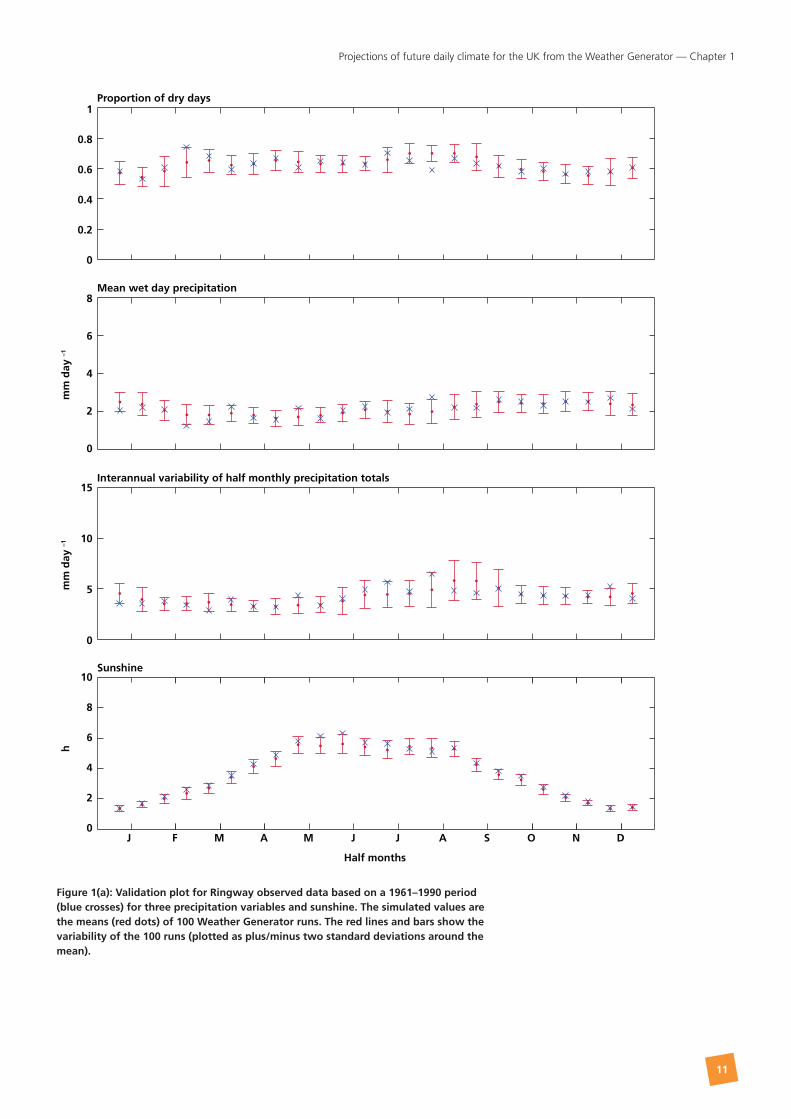
The performance of the WG in reproducing the 1961–1990 observations can be assessed using seasonal plots of weather variables. Figures 1(a) and (b) show an example of the WG fitted to the 1961–1990 daily observed weather data for Ringway (Manchester Airport). In Figures 1(a) and (b), the observed 30-yr average is within the two standard deviation range of the 100 generated sequences, each of 30 yr in length for all variables, for all half months of the year. Figure 2 shows examples of the performance of the WG in reproducing key rainfall statistics for Heathrow Airport, including the annual daily maximum rainfall. Further assessments of performance for rainfall extremes for a single site and across the whole UK are shown in the next section of this report. Maps and further diagnostics of performance are given in the Annex.

The WG can also produce generated sequences of hourly data. Many users will not require this feature. Those considering using hourly time series are referred to the Annex where it is discussed in more detail. The hourly component of the WG is essentially a temporal disaggregator of daily values based on observational data. The total or average of the data for the hourly variables will equal the daily values. The climate change component to any change comes principally from the changes applied at the daily timescale which in turn are based on the climate projections. This procedure has been adopted because there is little confidence in modelled climate at timescales less than daily.

11


Figure 1(a): Validation plot for Ringway observed data based on a 1961–1990 period (blue crosses) for three precipitation variables and sunshine. The simulated values are the means (red dots) of 100 Weather Generator runs. The red lines and bars show the variability of the 100 runs (plotted as plus/minus two standard deviations around the mean).

J F M A M J J A S O N D

Half months

Sunshine

Interannual variability of half monthly precipitation totals

Mean wet day precipitation

Proportion of dry days

mm

day

–1m

m d

ay –1

h

1

0.8

0.6

0.4

0.2

0

8

6

4

2

0

15

10

5

0

10

8

6

4

2

0

12


Figure 1(b): Validation plot for Ringway observed data based on a 1961–1990 period (blue crosses) for minimum and maximum temperature, vapour pressure and PET. The simulated values are the means (red dots) of 100 Weather Generator runs. The red lines and bars show the variability of the 100 runs (plotted as plus/minus two standard deviations around the mean).


Half months

Reference potential evapotranspiration

Vapour pressure

Maximum temperature

Minimum temperature

˚C˚C

hPa

mm

day

–1

20

15

10

5

0

-5

30

20

10

0

25

20

15

10

5

0

5

4

3

2

1

0

13


Figure 2: Performance of NSRP rainfall model in reproducing observed rainfall statistics for Heathrow. Calculated from 100 30-yr simulated series: NSRP 10/90% bounds.

0

0.5

1

1.5

2

2.5

Calendar Month

Mea

n d

aily

rai

nfa

ll (m

m)

1 2 3 4 5 6 7 8 9 10 11 12

1 2 3 4 5 6 7 8 9 10 11 12 1 2 3 4 5 6 7 8 9 10 11 12

1 2 3 4 5 6 7 8 9 10 11 121 2 3 4 5 6 7 8 9 10 11 12

Observed

NSRP mean

NSRP 10/90% bounds

0

5

10

15

20

25

30

35

40

Calendar Month

Var

ian

ce o

f d

aily

rai

nfa

ll (m

m2 )

0

0.1

0.2

0.3

0.4

0.5

0.6

0.7

0.8

0.9

Calendar Month

Pro

po

rtio

n o

f d

ry d

ays

0

1

2

3

4

5

6

7

8

9

Calendar Month

Skew

of

dai

ly r

ain

fall

0

0.05

0.1

0.15

0.2

0.25

0.3

0.35

Calendar Month

Au

toco

rrel

atio

n, L

ag 1

of

dai

ly r

ain

fall

14


2 Using the Weather Generator to produce extremes

Many users are engaged in assessments of changes in the severity and frequency of extremes and this is one of the most challenging aspects of climate research, beset by fundamental limitations and inadequacy in theory and practice. First of all, extremes are, by their nature, infrequent events, so that we only have small sample numbers from observational records of the most important extremes. This limits the power of statistical approaches to the estimation of extremes, and inevitably requires the user to estimate uncertainties or confidence limits around such estimates. Second, frequency analysis assumes stationarity in the observed data, and this is clearly not true for temperature (and possibly rainfall) extremes in the recent record. Third, the processes causing extremes (such as floods and droughts) are complex and their representation is at the limit of the current capability of climate models (see Annexes 3 and 5 from Murphy et al. 2009). Nonetheless, it is important to provide estimates of future extremes. The approach taken in UKCP09 is to use its WG to allow estimation of extremes and other properties of climate where credible, by generating long, stationary series to provide large statistical samples.

A range of extremes and derived properties may be generated using the WG. Table 1 provides some possible examples that have been used recently. Users can define their own specialist indices or measures of extremes and extract the values from WG series. They should follow the method of comparison of future values of their chosen index with the same index calculated from the control version of the WG generating baseline (1961–1990) climate, and wherever possible also validate this against their own observed data. To achieve this, when running the WG, users will be supplied with at least 100 30-yr generated sequences of the baseline climate and a similar number for their chosen 30-yr future period. Some widely used indices have been identified and can be extracted using the Threshold Detector (see the Annex). There are various types of weather indices or extremes that can be derived from the WG which are not available directly from the probabilistic projections, including maxima and minima (e.g. the median of annual maximum rainfall (Rmed)), threshold exceedances (e.g. occurrences of temperature above 28°C), spell lengths (e.g. mean dry spell length) and cumulative measures (e.g. GDD — cumulative growing season degree days).

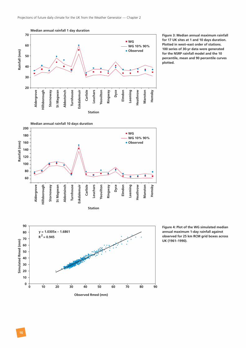
A crucial measure of rainfall extremes is the annual maximum daily rainfall. An example of what can be extracted from the UKCP09 WG is presented in Figure 3, showing the model performance in reproducing the median annual maximum one-day rainfall (Rmed).

15


Abbreviation* Quantity Notes

Rainfall indices

Rmed1, Rmed5, Rmed10

Annual maximum rainfall Median of annual maxima for 1, 5 and 10 day duration

CDD No. of consecutive dry days Threshold of 1 mm

SDII Simple daily intensity index (annual rainfall total on rain days (days with >1 mm of rain) / number of rain days)

RD Number of days per month having a rainfall >= 1 mm (rain days)

WD Number of days per month having a rainfall >= 10 mm (wet days)

CWD Maximum number of consecutive wet days each year/season (days)

Temperature indices

FD Number of days of air frost

FDG Number of days of ground frost Tmin < 2ºC

AETR Annual extreme temperature range (highest daily maximum — lowest daily minimum) (°C)

HWD Summer heat wave duration — Total days with maximum temperature >3°C above the 1961–1990 average for greater than five consecutive days (May to October)

CWD Winter cold wave duration — Total days with minimum temperature >3°C below the 1961–1990 average for greater than five consecutive days (November to April)

HWT Default threshold for heatwaves 30ºC Tmax and 15°C Tmin for two consecutive days

Twarm Hottest day of the year; numbers of days above specified thresholds

Tcold Coldest day of the year; numbers of days below specified thresholds

* Some of the abbreviations come from the STARDEX project (http://www.cru.uea.ac.uk/cru/projects/stardex/). More discussion of possible extreme indices is given by the WMO/CLIVAR Expert Team on Climate Change Detection and Indices, who also provide software for indices calculation (http://www.clivar.org/organization/etccdi/etccdi.php).

Table 1: Some of the extremes and indices that can be easily derived from output from the WG

To test the performance of the rainfall model across the UK, a 100-yr simulation was carried out using the 25 by 25 km Regional Climate Model (RCM) grid corresponding to the 1961–1990 period, and the Rmed calculated and compared with observations. This is shown in Figure 4 and shows good agreement. This is a powerful validation test, since the model is fitted only with a general sample statistic (the skewness), derived from all days with rainfall and then validated with the annual maxima only which were not explicitly used in the fitting.

16


Station

Station

WGWG 10% 90%Observed

WGWG 10% 90%Observed

Rai

nfa

ll (m

m)

Rai

nfa

ll (m

m)

Median annual rainfall 1 day duration

Median annual rainfall 10 days duration

70

60

50

40

30

20

200

180

160

140

120

100

80

60

Ald

erg

rove

Hill

sbo

rou

gh

Sto

rno

way

St M

agw

an

Ab

bo

tsin

ch

Turn

ho

use

Eskd

alem

uir

Car

lisle

Leu

char

s

Yeo

vilt

on

Rin

gw

ay

Dyc

e

Elm

do

n

Leem

ing

Hea

thro

w

Man

sto

n

Hem

sby

Ald

erg

rove

Hill

sbo

rou

gh

Sto

rno

way

St M

agw

an

Ab

bo

tsin

ch

Turn

ho

use

Eskd

alem

uir

Car

lisle

Leu

char

s

Yeo

vilt

on

Rin

gw

ay

Dyc

e

Elm

do

n

Leem

ing

Hea

thro

w

Man

sto

n

Hem

sby

y = 1.0305x – 1.6861

R 2 = 0.945

0

10

20

30

40

50

60

70

80

90

Observed Rmed (mm)

Sim

ula

ted

Rm

ed (

mm

)

0 10 20 30 40 50 60 70 80 90

Figure 3: Median annual maximum rainfall for 17 UK sites at 1 and 10 days duration. Plotted in west–east order of stations. 100 series of 30-yr data were generated for the NSRP rainfall model and the 10 percentile, mean and 90 percentile curves plotted.

Figure 4: Plot of the WG simulated median annual maximum 1-day rainfall against observed for 25 km RCM grid boxes across UK (1961–1990).

17


The Weather Generator perturbed with UK Climate Projections

Change Factors reproduces the daily weather variability simulated

directly by the Regional Climate Model.

The perturbations (referred to earlier as Change Factors) that will be applied to the WG (in UKCP09) will be taken from the probabilistic projections and joint probabilistic information developed in Chapters 4 and 5 of Murphy et al. 2009. This information is available for monthly, seasonal and annual time periods, at 25 by 25 km spatial resolution and for each of the seven future 30-yr periods (overlapping every 10 yr) from 2010–2039 to 2070–2099. The probabilistic projections and joint probabilities give ranges over which the climate (as described by precipitation, mean temperature, daily temperature range, vapour pressure and sunshine) is projected to change in the future (both in the mean and additionally for precipitation and temperature in variance, and for precipitation in skewness, proportion of dry days and lag-1 autocorrelation). As the WG works at the 5 km grid square scale, all squares within the same 25 by 25 km RCM grid box will have the same set of Change Factors. The 5 km grid squares which cross the boundaries of the larger 25 km RCM grid boxes (which are offset from the National Grid based 5 km squares) have been linearly interpolated from the values of the larger grid boxes.

The purpose of this section is to illustrate the way the WG will be perturbed. Observational data are neither long enough to assess whether the proposed way of perturbing the WG will work, nor do they contain a large change in climate when compared to that anticipated in the future. So, instead of using the observations, we use the base RCM integration (the member of the eleven RCMs, available through UKCIP, with the standard set of RCM parameter values — see Murphy et al. 2009 for more discussion on the perturbed physics experiments). For this exercise the WG was re-fitted to the control run period (model years 1961–1990) for selected 25 by 25 km grid boxes across the UK. Change Factors, for this exercise, were calculated from the relevant statistics from the 2070–2099 future and the control-run integrations (see the example later in Table 2). These were then applied to the WG calculated as either differences or ratios depending on the variable (see the Annex for how this is accomplished for the precipitation measures). For mean daily temperature and temperature range, changes were assumed to be the same for all five rainfall transitions within the WG (see Annex for a discussion of rainfall transitions).

3 Proving the perturbation of the Weather Generator for future periods works

18


As the WG generates the weather variables in sequence (see Annex), changes to precipitation will affect mean temperature and temperature range, and similarly changes to these variables will affect the generation of sunshine and vapour pressure. We need to ensure that future changes that occur for all non-precipitation variables are exactly the values prescribed from the future RCM integrations. To achieve this we modify the perturbations we apply to these variables to allow for the changes that will have occurred earlier in the generation sequence. This is best illustrated with an example: the selected perturbation for a summer month might be a 50% reduction in rainfall and 3ºC increase in mean temperature. From observations, dry summer months are generally warmer, so there will be a precipitation-related change in temperature of about +0.3ºC. In this example, the change in temperature is adjusted to 2.7ºC so in the generated sequences, the mean change will be equal to the perturbation defined by the Change Factor choice. This procedure becomes more complex for sunshine and vapour pressure, but is essential to ensure that the averages of the generated sequences reproduce the Change Factors developed in Murphy et al. 2009.

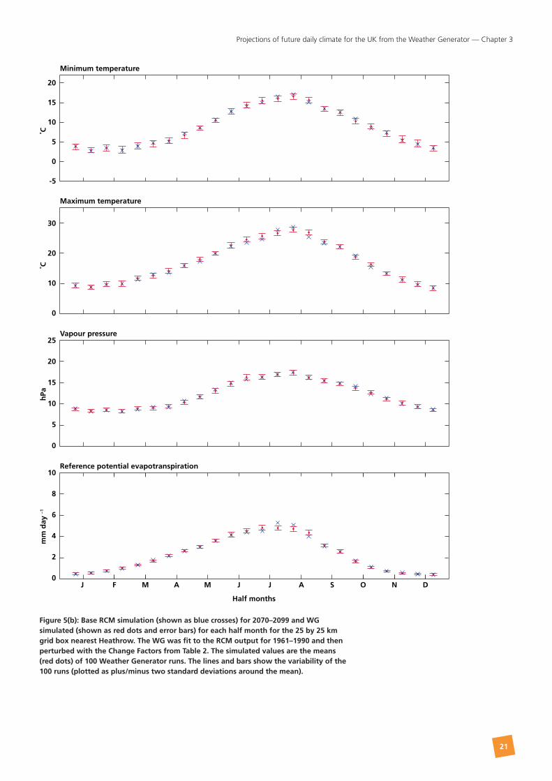
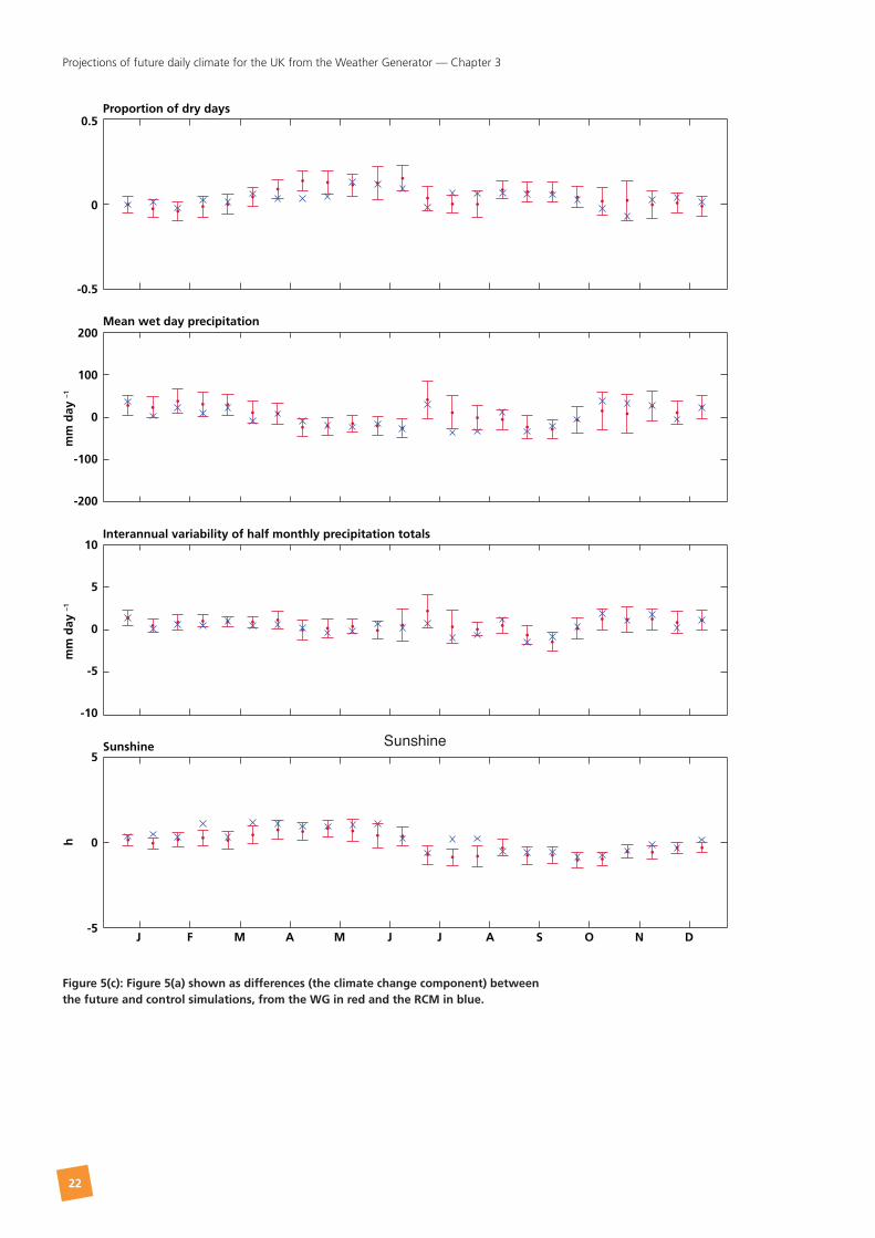
Figures 5(a) and (b) show plots for the RCM grid box including Heathrow Airport for the future using the perturbation procedure described above. In these plots we have the means and ranges of the 100 generated sequences, together with the crosses (for this one RCM simulation), which is the direct RCM average for the future 30-year period centred on the 2080s. We also show in this figure the differences (in other words the climate change component) compared to the RCM control run. For almost all variables and half months, the direct RCM future values (the crosses) are within the ranges generated by the WG. Table 2 gives the one set of Change Factors used in Figure 5 for the 25 by 25 km grid box encompassing Heathrow Airport.

At this point it is important to realise that for UKCP09 the WG has been fitted using observational data (see earlier and the Annex), then perturbed (with the Change Factors) according to the procedure just described. Using the WG fitted to observational data across the UK will better reflect local topographic and coastal influences on our weather than can be simulated by the RCM. These aspects will remain essentially unchanged in the future, so will be incorporated in the future generated sequences, to the extent that such influences are captured by daily weather data at the 5 km resolution.

19


Jan Feb Mar Apr May Jun Jul Aug Sep Oct Nov Dec

Precipitation average (mm)

1.20 1.16 1.07 0.99 0.79 0.79 0.96 0.89 0.73 1.17 1.30 1.07

Precipitation variance (mm)

1.49 1.40 1.61 1.22 0.84 1.22 0.97 1.27 0.57 1.80 1.89 1.33

Precipitation probability dry

1.03 1.02 1.18 1.13 1.43 1.56 1.14 1.41 1.36 1.02 0.91 1.14

Precipitation skew

0.90 0.96 1.22 1.25 1.36 2.00 0.76 1.33 0.90 1.24 1.13 1.24

Precipitation lag–1 correlation

1.10 0.87 0.99 1.02 0.88 0.95 1.12 1.09 0.92 1.11 0.99 1.04

Temperature average (°C)

3.08 2.76 3.61 2.90 3.46 3.72 4.50 5.08 4.44 3.78 3.49 2.78

Temperature variance (°C)

0.90 0.80 1.14 1.06 1.04 1.37 2.32 1.55 1.50 1.22 0.93 0.98

Temperature range (°C)

0.26 0.50 0.38 0.17 0.49 0.67 0.74 0.98 0.76 0.35 0.18 –0.09

Sunshine average (h)

0.57 0.93 0.94 1.18 1.06 0.67 –0.21 –0.15 –0.58 –0.80 –0.30 –0.04

Vapour pressure average (hPa)

1.64 1.32 1.83 1.49 2.07 2.08 2.20 2.74 2.82 2.70 2.17 1.54

Table 2: The Change Factors used for the Heathrow example in Figure 5.

20



Half months

Sunshine




mm

day

–1m

m d

ay –1

h

1

0.8

0.6

0.4

0.2

0

8

6

4

2

0

15

10

5

0

15

10

5

0

Figure 5(a): Base RCM simulation (shown as blue crosses) for 2070–2099 and WG simulated (shown as red dots and error bars) for each half month for the 25 by 25 km grid box nearest Heathrow. The WG was fit to the RCM output for 1961–1990 and then perturbed with the Change Factors from Table 2. The simulated values are the means (red dots) of 100 Weather Generator runs. The lines and bars show the variability of the 100 runs (plotted as plus/minus two standard deviations around the mean).

21



Half months


Vapour pressure

Maximum temperature

Minimum temperature

˚C˚C

hPa

mm

day

–1

20

15

10

5

0

-5

30

20

10

0

25

20

15

10

5

0

10

8

6

4

2

0

Figure 5(b): Base RCM simulation (shown as blue crosses) for 2070–2099 and WG simulated (shown as red dots and error bars) for each half month for the 25 by 25 km grid box nearest Heathrow. The WG was fit to the RCM output for 1961–1990 and then perturbed with the Change Factors from Table 2. The simulated values are the means (red dots) of 100 Weather Generator runs. The lines and bars show the variability of the 100 runs (plotted as plus/minus two standard deviations around the mean).

22



Half months

Sunshine




mm

day

–1m

m d

ay –1

h

0.5

0

-0.5

200

100

0

-100

-200

10

5

0

-5

-10

5

0

-5

Sunshine

Figure 5(c): Figure 5(a) shown as differences (the climate change component) between the future and control simulations, from the WG in red and the RCM in blue.

23



Half months


Vapour pressure

Maximum temperature

Minimum temperature

˚C˚C

hPa

mm

day

–1

10

8

6

4

2

0

10

8

6

4

2

0

5

0

-5

5

0

-5

Figure 5(d): Figure 5(b) shown as differences (the climate change component) between the future and control simulations, from the WG in red and the RCM in blue.

24


The Weather Generator projects changes in temperature and rain-

fall variables and various derived indices which are not directly avail-

able from the climate model output. These changes are driven by

Change Factors from the climate model analysis, and the Weather

Generator outputs are therefore consistent with the climate model

Probability Distribution Functions.

Amongst the most notable changes related to temperature are increases in heat wave frequency in the south and east, and major increases in maximum temperatures nation wide, along with reductions in frost days. Amongst changes related to rainfall are increases in dry spell frequency related to summer drying and increases in the annual wettest day amounts.

The Weather Generator has been run for a control period corresponding to the baseline (1961–1990) and future projections to estimate the changes in key climate indices and to check that the changes are consistent with those from the climate model PDFs where possible. The method involves first running the WG for the control (i.e. fitted to observed statistics) 100 times with a random seed, thus generating an ensemble of 100 different time series of length 30 yr. Then the WG is run once for each of 1000 climate model output variants for a future projection. The variants are sampled randomly across the PDF. Differences between climate indices calculated from this future ensemble and the baseline ensemble are then derived. This strategy is followed because the variability in the WG baseline is small relative to the variation in the future climate PDF obtained from the climate model outputs, more so for more distant futures.

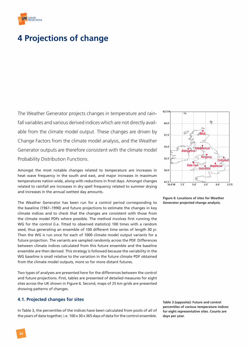
Two types of analyses are presented here for the differences between the control and future projections. First, tables are presented of detailed measures for eight sites across the UK shown in Figure 6. Second, maps of 25 km grids are presented showing patterns of changes.

4.1. Projected changes for sites

In Table 3, the percentiles of the indices have been calculated from pools of all of the years of data together, i.e. 100 x 30 x 365 days of data for the control ensemble.

4 Projections of change

10.0˚W 7.5˚ 5.0˚ 2.5˚ 0.0˚ 2.5˚E47.5˚

50.0˚

52.5˚

55.0˚

57.5˚

60.0˚

62.5˚N

Heathrow Yeovilton

Coltishall

Dale Fort

Ringway

AldergroveEskdalemuir

Wick

Figure 6: Locations of sites for Weather Generator projected change analysis.

Table 3 (opposite): Future and control percentiles of various temperature indices for eight representative sites. Counts are days per year.


Observed 1961–1990 2080s Medium

50% 10% 50% 90% 10% 50% 90%Heatwaves (2 days with Tmax>29ºC and Tmin>15ºC )

Heathrow 0 0 0 0 1 7 22

Yeovilton 0 0 0 0 0 5 17

Coltishall 0 0 0 0 0 1 9

Dale Fort 0 0 0 0 0 0 5

Ringway 0 0 0 0 0 1 8

Aldergrove 0 0 0 0 0 0 3

Eskdalemuir 0 0 0 0 0 0 2

Wick 0 0 0 0 0 0 0

Hot days (>28ºC)

Heathrow 2 0 2 6 9 27 60

Yeovilton 1 0 0 2 5 21 52

Coltishall 0 0 0 1 2 11 37

Dale Fort 0 0 0 0 0 6 24

Ringway 0 0 0 1 1 9 29



Wick 0 0 0 0 0 0 3

Hot days (>25ºC )

Heathrow 15 8 15 23 44 76 109

Yeovilton 8 3 7 13 32 64 96

Coltishall 7 1 4 9 18 42 77

Dale Fort 0 0 0 2 5 20 49

Ringway 4 0 3 7 14 35 65

Aldergrove 0 0 0 2 5 17 40


Wick 0 0 0 0 0 1 8

Frost days (Tmin <= 0ºC )

Heathrow 39 26 41 56 3 11 26

Yeovilton 54 30 44 59 3 12 27

Coltishall 49 33 49 65 3 13 29

Dale Fort 11 6 14 23 0 2 9

Ringway 43 31 44 60 4 13 28

Aldergrove 44 30 43 57 4 13 28

Eskdalemuir 94 80 98 115 16 38 64

Wick 52 33 47 62 6 18 35

Annual highest Tmax (ºC )

Heathrow 29.9 27.8 29.5 31.7 32.0 35.7 40.2

Yeovilton 28.4 26.3 27.9 30.0 30.9 34.5 39.3

Coltishall 28.0 25.5 27.2 29.1 29.2 32.3 36.2

Dale Fort 24.8 23.0 24.6 26.7 27.2 30.5 35.1

Ringway 27.6 25.0 26.8 29.0 29.3 32.5 36.7

Aldergrove 24.2 23.2 25.0 27.0 27.1 30.2 34.1

Eskdalemuir 24.8 22.1 23.9 26.2 26.1 29.5 33.8

Wick 21.6 20.4 21.8 23.7 23.4 26.0 29.3

26


The mean observed values are also shown to enable the WG performance for the control to be assessed. The sites are listed in order from south to north.

Very few hot days (daily maximum temperature above 28ºC) or heatwaves (days above 29ºC) are found in the observations or control WG outputs, so days above 25ºC have also been calculated. In both cases, major increases in day counts are found for the future projection.

In Table 4, there are significant increases in the 10 day dry spell frequency associated with summer drying. Increases for the 20 day spells are more limited. It should be noted that the WG and climate models both have limited capabilities of reproducing these very long dry spells — see the Annex for further details.

Observed 1961–1990 2080s Medium

10% 50% 90% 10% 50% 90%

Dry spells (10 day+)

Heathrow 9 5 9 12 8 11 15

Yeovilton 9 4 7 10 6 10 13

Coltishall 8 5 9 12 8 11 15

Dale Fort 7 2 4 7 4 7 10

Ringway 7 2 4 7 3 6 9



Wick 4 1 3 6 2 4 7

Dry spells (20 day+)

Heathrow 1 0 1 2 1 2 4

Yeovilton 1 0 1 2 1 2 4

Coltishall 1 0 1 3 1 2 5

Dale Fort 1 0 0 1 0 1 3

Ringway 1 0 0 1 0 1 2



Wick 0 0 0 1 0 0 1

Rmed 1 day (Median annual maximum rainfall, mm)

Heathrow 38 31 35 39 34 41 50

Yeovilton 33 32 34 37 35 41 51

Coltishall 35 31 34 37 32 38 46

Dale Fort 33 33 36 39 38 43 51

Ringway 38 31 34 36 33 39 46

Aldergrove 31 31 34 36 34 39 46

Eskdalemuir 60 51 55 59 58 66 75

Wick 29 29 30 32 32 37 42

Table 4: Future and control percentiles of various rainfall indices for eight representative sites. Counts are days per year.

27


* Please note that these maps are not reproducible from the User Interface.

4.2. Projected patterns of change from the Weather Generator

Ensembles of Weather Generator outputs were produced on a 25 km grid across the UK in a similar manner as for the sites. Change Factors are available on the 25 km grid, and the observed statistics were averaged from the 5 km grid resolution to match. A sample of the outputs are shown here.

The largest increase in hot days is found in the south east of England (see Figure 7), where for the 50th percentile (or median case) an increase from around 20 to more than 50 days per year is expected. The maps should be interpreted as showing the differences (increases) in frequency of hot days between the same percentile. For example, for the 90th percentile maps, they show the number of days per year which is exceeded on average in only 10% of years.

A corresponding decrease in frost days is found as shown in Figure 8. Substantial decreases are found across the UK, except where they are already close to zero (e.g. near coasts).

Finally, changes in the pattern of dry spells are shown in Figure 9, where modest increases are found across the country and substantial increases in the south and east associated with summer drying.

Number of hot days

0 15 30 45 60 75 90 105

10th percentile:Likely to be exceeded every 9 in 10 yr

50th percentile:Likely to be exceededevery 5 in 10 yr


Figure 7: Numbers of hot days (above 25°C) annually estimated by the Weather Generator, for control scenario (top row) and 2080s medium emissions projection (bottom row). The left hand column is the10th percentile of the distribution of hot days, the middle column the 50th and right hand column the 90th.

28


Figure 9: Numbers of dry spells longer than 10 days annually estimated by the Weather Generator. Rows and columns as for Figure 7.

0 3 6 9 12 15

Number of dry spells




Number of frost days

0 30 60 90 120 150 180




Figure 8: Numbers of frost days (air temp below 0°C) annually estimated by the Weather Generator. Rows and columns as for Figure 7.

29


Limitations of the Weather Generator include that it does not

simulate some extremes well; and does not give spatial consistency

across grid squares. It also assumes that the observed relationships

between weather variables will remain the same in the future.

The Weather Generator outputs are subject to a number of limitations which must be borne in mind when using them. The most important of these are outlined here, and expanded upon further in the Annex and in the UKCP09 User Guidance.

5.1 Lack of physical basis

The Weather Generator method relies on learning the detailed behaviour of weather from observed weather data and using it in statistical relationships (the IVRs described in Chapter 1). Although these IVRs can be interpreted with some physical sense (e.g. dry days in summer will on average be warmer than wet days), there is no explicit basis in physics or meteorology within the WG, and therefore no guarantee that the generated series, particularly under a changed climate, will always reproduce the correct weather behaviour. This is likely to be the case for some weather extremes (e.g. hot dry spells), particularly when future climates produce conditions outside of the range of those previously observed, and care must be taken to (a) compare the future WG series in a relative sense with WG baseline series (based on the period 1961–1990) and (b) check how well the WG performs for the baseline period of observational data.

However, the WG is heavily constrained not just by the IVRs related to baseline observed climate, but also by the use of Change Factors derived from the probabilistic projections applied to the WG. This ensures that the overall statistics (e.g. averages and standard deviation of the variables’ distributions) are the same as those estimated by the UKCP09 methodology. The use of the observationally-based IVRs for future time periods may appear a significant limitation, but it is the same assumption as made in all statistically-based downscaling techniques.

There is also an overall hierarchy in the way that the WG variables are generated, so that the rainfall and temperature variables are generated first, and are therefore subject to less error than subsequent variables such as vapour pressure and sunshine hours.

5 Limitations of the Weather Generator

30


5.2 The WG and the RCM grid resolution (5 km versus 25 km)

The WG operates at a 5 km resolution, although the climate Change Factors are developed using the UKCP09 probabilistic projections at a 25 by 25 km resolution. In both cases, these are the highest resolution data available. It is of course recognised that there is variability (or noise) in the spatial data sets, arising from various sources, which means that there is a limit to the resolution which is meaningful for such analyses, as it can give illusory detail or variation. However, in the case of the UKCP09 WG application, the resolution is justified, as there is an important and significant spatial signature in the long-term observational weather and climate data which is captured by the 5 km grid.

The 5 km grid provides useful information on how the long-term average statistics of weather vary across the country, derived from 30 yr of observations from numerous weather stations. The variation across the country is resolved at 5 km because most weather variables (e.g. rainfall and temperature) depend on the ground surface elevation and geography in a systematic way, and at a similar space scale. It is important to include this variation in the WG so that its outputs can be used for 5 km-square-based locations. For example, the rainfall on a mountainous 5 km grid square will be considerably higher than on a neighbouring low-lying square. In the WG, as in RCM simulations, each grid square and grid box have average elevations for the areas. The dependence of rainfall and temperature on the topography is likely to be essentially the same in the future as it has well understood meteorological causes based in thermodynamics, so this downscaling provides our current best estimate of the spatial variation across the country. In any case, if such a method was not made available and followed, users may apply their own, different downscaling procedures, thus causing inconsistency and confusion.

5.3 Point vs spatial data

The UKCP09 WG is based on the concept (as discussed in Kilsby et al. 2007) of a point-based process. The implication of this is that if a series is generated for a neighbouring (5 km) square to one already generated, there will be no correlation in time between the two series (e.g. at any given time, it may be raining in one square and not the other). Whilst rainfall models have been developed which can generate consistent space-time series for use in, for example, large river basin flood models, these are considered too complex for use in UKCP09 at this time.

If time series are required for a region, rather than for a point, then an approximation may be used where the user can designate a larger region (up to 1000 km2), and the coefficients used to generate weather for these larger than a single-square regions are taken to be the spatial averages of all the WG coefficients (the means, standard deviations and IVRs) for the selected squares. Care must be taken in the interpretation of this series however, as it still corresponds to a single point, but a point which is representative, on average, of the region. The weather variables in the series are not areal-averaged values. Care must also be taken that a homogeneous region is chosen, avoiding for example, large differences in elevation which may cause averaging of very different rainfall rates across the region.

For regions larger than 1000 km2, we recommend direct use of the 11-member RCM simulations, available through LINK, when users require real spatial

31


correlation in the weather. All 11 RCM simulations should be used to build up a range of possible changes. For example, for many hydrological assessments (e.g. flooding on the River Thames) spatial correlation is essential. The 25 km resolution daily outputs from the 11-member RCMs could be directly input to an appropriate catchment model (see the UKCP09 User Guidance for further information on using the 11-member RCM outputs). An alternative approach is to use a customised space-time version of the NSRP rainfall model used in the UKCP09 WG. Such models are widely used in research applications, and are capable of representing hourly rainfall fields over catchments up to some 10,000 km2. Such models have not been extended to provide outputs for the other weather variables available in UKCP09. With both possibilities, it should be realised that the concept of the UKCP09 PDFs no longer applies.

In another application (e.g. building performance design), spatial correlation is not important. Here the WG could be used, for a number of 5 by 5 km grid squares across the selected region. A measure of building performance (e.g. the period air conditioning has to be used) can be calculated for each of the 100 simulations and compared to performance in the baseline period. Spatial correlation is not important in this example and the distribution of the performance measure (expressed, for example, as a probabilistic distribution) will be extremely similar for adjacently-located 5 by 5 km grid squares.

5.4 Hourly data

The rainfall and other variables in the WG are primarily estimated at the daily level, with simple disaggregation rules used for generating hourly resolution data that might be required for certain types of impact models. These rules are taken from the current climate and fixed for future time periods. This means that new types of hourly weather behaviour (e.g. more intense thunderstorms) will not be explicitly reproduced by the WG for future periods. This must be recognised as an important limitation of the WG approach, although such information is also not currently available from climate models either.

5.5 Extreme events

The difficulties of generating extreme weather series have already been noted. Considerable effort has been devoted to improving the stochastic rainfall model’s ability to reproduce extreme rainfall amounts, but some limitations should be briefly discussed. Very long series may be generated (e.g. 10,000 yr), which may be used in principle to estimate long return period (or low annual exceedance probability, AEP) extremes, for example the 100 yr (1% AEP) rainfall event.

However, whilst there may be sufficient data in this 10,000 yr sample to estimate this event, and the series is stationary, care must be taken in interpreting this quantity, since it is derived from an imperfect model, which has been fitted (and must be validated by the user) using a much shorter observed record (typically 30 yr of rainfall data, 1961–1990). Daily rainfall extreme statistics for return periods longer than, say, 10 yr should therefore be used with caution, and the user is advised to carry out uncertainty analysis using the 100 generated WG series provided. More detailed advice is given in the Annex and the UKCP09 User Guidance and UKCP09 Weather Generator Guidance.

Hourly extreme statistics are subject to even more uncertainty, and return periods beyond 5 yr should be used with caution. In all cases, the user should bear in

32


mind the uncertainty of frequency estimates from observed data arising from natural variability in the first instance. For example, hourly estimates of extreme rainfall derived using the Flood Estimation Handbook (NERC, 1999) may be based on observed series as short as 15 yr in length.

One particular type of extreme is spells of similar weather patterns, that lead to heatwaves/droughts and/or cold spells. These events relate to the persistence of specific weather types, often referred to by climatologists as blocking or weather regimes, and are particularly important with respect to not only heatwaves/droughts (e.g. the 1976 summer drought) but also to exceptionally cold winters (e.g. the winter of 1962–1963). Performance for such events is particularly difficult to reproduce, and both the WG and climate models do not adequately reproduce some significant features of these phenomena. It is likely that the WG will not simulate the very extreme examples (the upper and lower 1–2% of any distribution) of these events very well. In theory, it is possible to improve their generation within the WG by the use of more complex statistical distributions, but the difficulty is then how to perturb the additional coefficients, as it is well known that GCMs (and hence the RCMs used in UKCP09) have not, historically, simulated blocking well either (see Annexes 4 and 5 of Murphy et al. 2009).

5.6 Long-term variability

The WG is based on two models with time scales of one day to one month (NSRP model) and 1–2 days (auto-regressive model for the other variables). The models are made to follow the average seasonality (using half-month long-term averages), but variability (on interannual and inter-decadal timescales) on time scales longer than a few weeks is not explicitly represented. The NSRP cluster type of model performs better than Markov type models (Gregory et al. 1992, 1993), and validations of the NSRP annual aggregated outputs against observational data are reasonable, as shown in Figure 10 .

900800700600500400

25

20

15

10

5

0

Annual rainfall (mm)

642.7 98.22 100644.4 96.32 100

Mean StDev N

ObservedWeather Generator

Frequency distribution of annual rainfall

Perc

ent

Figure 10: Comparison of counts (y axis) of annual rainfall (x axis) at Durham for 100 yr of observations and WG output for the nearest 5 km square. Normal distributions have been fitted. The means and standard deviations are 643 and 98 mm for the observed case and 644 and 96 mm for the WG.

33


However, the lack of explicit controls on autocorrelation at high aggregations of one or more years means that longer-term variability may not be well represented by the WG. This may be important for some applications, e.g. for water resource models, when reductions in rainfall produced by a run of two or three drier than average seasons, will not be adequately simulated by the WG. The current generation of climate models also imperfectly reproduces such long-term variability. The user is therefore advised to use alternative means of modulating the long-term properties of the series if this is crucial, e.g. using hierarchical or weather type models such as Wilby et al. 2002 and Fowler et al. 2005.

34

Projections of future daily climate for the UK from the Weather Generator — References

Cowpertwait, P. S. P., O’Connell, P. E., Metcalfe, A. V. & Mawdsley, J.A. (1996). Stochastic point process modelling of rainfall. 2. Regionalisation and disaggregation. Journal of Hydrology, 175, 47–65.

Cowpertwait P. S. P., Kilsby, C. G. & O’Connell, P. E. (2002). A space-time Neyman-Scott model of rainfall: Empirical analysis of extremes. Water Resources Research, 38. (doi:10.1029/2001WR000709).

Ekström, M., Jones, P. D., Fowler, H. J., Lenderink, G., Buishand, A. & Conway, D. (2007). Regional climate model data used within the SWURVE project. 1: Projected changes in seasonal patterns and estimation of PET. Hydrology and Earth System Sciences, 11, 1069–1083.

Fowler, H. J., Kilsby, C. G., O’Connell, P. E. & Burton, A. (2005). A weather-type conditioned multi-site stochastic rainfall model for the generation of scenarios of climatic variability and change. Journal of Hydrology, 308, 50–66.

Gregory, J. M., Wigley, T. M. L. & Jones, P. D. (1992). Determining and interpreting the order of a two-state Markov chain: Application to models of daily precipitation. Water Resources Research, 28, 1443–1446.

Gregory, J. M., Wigley, T. M. L. & Jones, P. D. (1993). Application of Markov models to area-average daily precipitation series and interannual variability in seasonal totals. Climate Dynamics, 8, 299–310.

Hutchinson, M. F. (1986). Methods of generation of weather sequences. In (A.H. Bunting Ed.) Agricultural Environments C.A.B. International, Wallingford, 149–157.

Kilsby, C. G., Jones, P. D., Burton, A., Ford, A. C., Fowler, H. J., Harpham, C., James, P., Smith, A. & Wilby, R. L. (2007). A daily Weather Generator for use in climate change studies. Environmental Modelling and Software, 22, 1705–1719.

Muneer, T. (2004). Solar Radiation and Daylight Models, Elsevier Butterworth-Heineman.

Murphy, J. M., Sexton, D. M. H., Jenkins, G. J., Booth, B. B. B., Brown, C. C., Clark, R. T., Collins, M., Harris, G. R., Kendon, E. J., Betts, R. A., Brown, S. J., Humphrey, K. A., McCarthy, M. P., McDonald, R. E., Stephens, A., Wallace, C., Warren, R., Wilby, R., Wood, R. A. (2009). UK Climate Projections Science Report: Climate change projections. Met Office Hadley Centre, Exeter, UK. 192pp.

NERC (1999). Flood Estimation Handbook, ISBN 094854094X, Centre for Ecology and Hydrology, Five Volumes.

Richardson, C. W. (1981). Stochastic simulation of daily precipitation, temperature, and solar radiation. Water Resources Research, 17, 182–190.

Srikanthan, R. & McMahon, T. A. (2001). Stochastic generation of annual, monthly and daily climate data: A review. Hydrology and Earth System Sciences, 5, 653–670.

Wilby, R. L., Conway, D. & Jones, P. D. (2002). Prospects for downscaling seasonal precipitation variability using conditioned Weather Generator parameters. Hydrological Processes, 16, 1215–1234.

Wilks, D. S. & Wilby, R. L. (1999). The weather generation game: a review of stochastic weather models. Progress in Physical Geography, 23, 329–357.

6 References

35


The basic structure, performance and application of the Weather

Generator are given in the main body of this report. More details

of the models, fitting and perturbation methodology are given in

this Annex.

1. Rainfall model

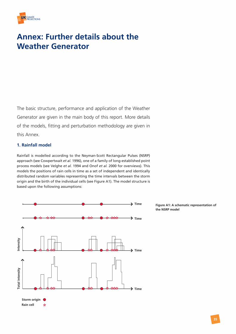
Rainfall is modelled according to the Neyman-Scott Rectangular Pulses (NSRP) approach (see Cowpertwait et al. 1996), one of a family of long-established point process models (see Velghe et al. 1994 and Onof et al. 2000 for overviews). This models the positions of rain cells in time as a set of independent and identically distributed random variables representing the time intervals between the storm origin and the birth of the individual cells (see Figure A1). The model structure is based upon the following assumptions:

Annex: Further details about the Weather Generator

Figure A1: A schematic representation of the NSRP model

Time

Time

TimeInte

nsi

ty

TimeTota

l in

ten

sity

Storm origin

Rain cell

36

Projections of future daily climate for the UK from the Weather Generator — Annex

• storm origins arrive in a Poisson process with the arrival time represented by a parameter l;

• each storm origin generates a (Poisson) random number n of raincells separated from the storm origin by time intervals that are each exponentially distributed with parameter b;

• the duration of each raincell is exponentially distributed with parameter h;

• the intensity of each raincell is exponentially distributed and represented with a parameter x;

• the rainfall intensity is equal to the sum of the intensities of all the active cells at that point.

The parameters of the NSRP model can be summarised as follows:

1. l–1 the average waiting time between subsequent storm origins (h),

2. b–1 the average waiting time of the raincells after the storm origin (h),

3. h–1 the average cell duration (h),

4. n–1 the average number of cells per storm,

5. x–1 the average cell intensity (mm/h).

The model parameters are different for each month of the year. Analytical expressions have been derived for expected values of various rainfall statistics (e.g. mean rainfall rate, proportion of dry days) in terms of these model parameters, and these are used to estimate (or fit) sets of parameter values corresponding to observed rainfall statistics. A procedure is followed where an objective function is defined using the differences between the expected and actual values of the rainfall statistics. The parameter space is then searched and the objective function minimised using an optimising algorithm. Robust and accurate fits to the lower order moments (mean, variance) are generally obtained, and much development has been carried out to improve the model performance for extremes using the skewness in fitting.

The UKCP09 version uses the following daily rainfall statistics in fitting: mean rainfall amount, the proportion of dry days, the variance and skewness of daily rainfall amounts and the lag-1 autocorrelation (see Cowpertwait et al. 2002 and Kilsby et al. 2007 for definition of these terms). The lag–1 autocorrelation coefficient helps in the fitting of persistent events such as long dry spells. For UKCP09, the estimation of the necessary rainfall statistics uses the daily gridded precipitation dataset developed by Perry and Hollis, 2005a, b and Perry, 2006 covering the UK at 5 km resolution for the period 1961–1990. This daily dataset uses elevation and eastings/northings in the interpolation of the daily station observations. For further details about the accuracy of the interpolations see the above references.

2. Generating the other variables

Once the precipitation sequence has been generated, the other variables are generated, maintaining the relationships within and between the variables (IVRs). This second component to the WG is developed from the statistics of observed daily station data, as gridded data similar to precipitation are not yet available. A network of 115 stations across the UK has been used (see Figure 2) and for UKCP09 purposes data for the period 1961–1995 have been used. The fitting takes into account the seasonal cycle and the conditioning by rainfall so considers five rainfall transition states (previous day(s) Dry/current day Dry DD and DDD, previous day Wet/current day Wet WW, DW and WD).

37


The seasonal cycles of both the mean and the standard deviation of all four variables (mean temperature, diurnal temperature range and vapour pressure) are removed by subtracting the mean and dividing by the daily standard deviation. In some instances temperature data is not quite normally distributed so a power transform to normality (Wilks, 2006) is applied prior to normalising to help improve the modelling accuracy. For sunshine, we have modified the generation procedure used in Kilsby et al. (2007), as daily totals are not normally distributed due to the large proportion of zero sun days. This problem has been addressed by utilising a latent Gaussian variables technique (Durban and Glasbey, 2001) where the input variable is first transformed to the upper part of the Gaussian distribution, the lower part (i.e. below a threshold) of the same distribution corresponds to the zero sun days. This has the advantage that the existing auto-regression technique can be retained.

Daily mean temperature and temperature range can be recombined to calculate mean daily maximum and minimum temperature. For both daily mean temperature and range, the residual time series are modelled as first-order autoregressive processes. To accommodate the five transitions, five equations and associated regression and correlation coefficients are calculated. Together these cross and auto-correlations between and within variables, respectively, have been referred to earlier as the Inter-Variable Relationships (IVRs), and as noted earlier these are assumed not to change in the future. The models are:

Dry Periods (current day dry, previous day dry): Ti = a1 Ti-1 + a2 Si-1 + b1 + e ; Ri = a3 Ri-1 + a4 Si-1 + b2 + e

Dry Periods (current day dry, previous day dry, day before dry): Ti = a5 Ti-1 + a6 Si-1 + b3 + e ; Ri = a7 Ri-1 + a8 Si-1 + b4 + e

Wet Periods (current day wet, previous day wet): Ti = a9 Ti-1 + b5 + e ; Ri = a10 Ri-1 + b6 + e

Dry/Wet Transition (current day wet, previous day dry) Ti = a11 Ti-1 + a12 Pi + b7 + e ; Ri = a13 Ri-1 + a14 Pi + b8 + e

Wet/Dry Transition (current day dry, previous day wet) Ti = a15 Ti-1 + a16 Pi-1 + b9 + e; Ri = a17 Ri-1 + a18 Pi-1 + b10 + e

All the weights (a1–a18, b1–b10) have been determined by multiple linear regression analysis using observed data. Ti, Ri and Pi are used to indicate mean temperature, range and precipitation on day i, and suffix i-1 indicates the previous day’s value. To help increase modelling accuracy the previous day’s sunshine, indicated by Si-1 is added to DD and DDD. All the e’s are independent standard normal (Gaussian) variables which will be scaled by the degree of fit or explained variance of each regression and are selected randomly when the models are used in simulation (i.e. weather generation) mode.

The remaining variables (X) have been determined by regression analyses of the form:

Xij = cj + dj Pi + ej Ti + fj Ri + gj Xi–1,j + e

where j = 1,2 corresponds to vapour pressure and sunshine duration. This general form ensures that the simulated data will have the correct autocorrelation structure. Correlations between these two variables and precipitation, temperature and temperature range (which are generally quite high) will also be

38


correctly simulated, and correlations between vapour pressure and sunshine will arise naturally through the common dependencies on Pi, Ti and Ri. Fitting the non-rainfall part of the WG results in many thousands of parameters, which include: the means and standard deviations for each half month for each transition; the regression weights in all the above equations and the variance explained by each regression, which determines the size of the random component added at various stages in generation. Half months are used to better approximate the annual cycle of non-rainfall variables.

For UKCP09, all the weather statistics (means and standard deviations of all the variables and the additional measures for precipitation) and all the IVRs are available on the 5 by 5 km squares for precipitation or have been interpolated to this grid, from estimates at the 115 sites in Figure A2, using topographic variables (elevation, eastings, northings and distance from the coast). This enables the WG to be used for any 5 by 5 km square across the UK. In order to ensure that estimation is for the average elevation of each 5 km square, average temperature is adjusted to be the average for the 1961–1990 period (using Appendix 7 of UKCIP02, an earlier version of Perry and Hollis, 2005a, b). Differences between the generated data and averages from individual stations will depend on the elevation of the station within the square and possible rain-shadow effects. As noted in Murphy et al. 2009, the WG requires daily station series (for temperature, sunshine and vapour pressure) of at least 30 yr in length. Such series (see Figure A2) are less available in western Britain, particularly in Northern Ireland and parts of Scotland.

At the end all generated variables are transformed back to absolute values using the adjusted means (with the Change Factors) and unaltered standard deviations (except for mean temperature). Potential evapotranspiration (PET) is then calculated using the FAO-modified version of the Penman’s formula (given in Ekström et al. 2007, which is in turn based on Allen et al. 1994). This method is essentially the same as the Met Office calculation formula used within MORECS (Hough and Jones 1997), but we assume that each square is covered by short grass. Direct and diffuse radiation are calculated from formulae given by Muneer, 2004, based principally on the daily sunshine amounts.

3. Further validation

The Weather Generator has been validated using the 1961–1990 rainfall fields for the statistics used in fitting as well as the Rmed (median annual maximum rainfall). This validation used the 25 km grid across the UK, and scatter plots are shown in Figure A3 to demonstrate goodness of fit. The statistics are generally fitted very well, with the exception of skewness. Skewness is an important measure of the proportion of high intensity rainfall, but is rather variable spatially due to the sensitivity of the statistic to the occurrence of one or two heavy rainfall events in the 30 yr of record. This inaccuracy in turn limits the WG capability for reproduction of extremes.

10.0˚W 7.5˚ 5.0˚ 2.5˚ 0.0˚ 2.5˚E47.5˚

50.0˚

52.5˚

55.0˚

57.5˚

60.0˚

62.5˚N

Figure A2: Station distribution map of the 115 sites.

39


Rainfall: Mean

y = 0.9972x – 0.0026R2 = 0.9898

0

2

4

6

8

10

12

0 2 4 6 8 10 12Observed (mm / day)

Sim

ula

ted

(mm

/ d

ay)

Rainfall: Daily Variance

y = 0.9125x + 1.4954R2 = 0.9797

0

50

100

150

200

250

0 50 100 150 200 250 300Observed (mm2)

Sim

ula

ted

(mm

2 )

Rainfall: Proportion Dry Days

y = 1.0089x – 0.0077

R2 = 0.9611

0.2

0.3

0.4

0.5

0.6

0.7

0.8

0.9

0.2 0.3 0.4 0.5 0.6 0.7 0.8 0.9Observed

Sim

ula

ted

Rainfall : Skewness

y = 0.6984x + 0.8005R2 = 0.7126

0

1

2

3

4

5

6

7

8

9

0 2 4 6 8 10 12Observed

Sim

ula

ted

Rainfall : Autocorrelation

y = 0.944x + 0.0051R2 = 0.8837

0

0.1

0.2

0.3

0.4

0.5

0.6

0 0.1 0.2 0.3 0.4 0.5 0.6Observed

Sim

ula

ted

Figure A3: Plots of simulated versus observed daily rainfall statistics used in fitting the NSRP model for all 25 by 25 km UK grid boxes for all months.

40


4. Discussion of perturbation methodology

Change Factors are obtained from the UKCP09 probabilistic projections on a calendar month basis and are multiplicative for rainfall statistics and temperature variance and additive for other climate variables. For rainfall, these are taken directly as ratios for the mean (M), variance (Var) and skewness (S) of daily rainfall, a logit transformation for proportion of dry days (PDry) and Fisher Z for lag-one autocorrelation (L1AC) to ensure linearity across the range of values 0:1 for PDry and –1:1 for L1AC. These transformations ensure that the perturbed values stay within the known physical bounds.

The following equations are used to apply the calculated change fields (a) for a general variable P using a transformation function X (using the suffix GCM to indicate climate model values):

PFut

PObs

α =

X(PDryFut) X(PDryGCMFut)

X(PDryObs) X(PDryGCMCon)

X(PDry) = PDry

1 – PDryα =

X(PDryGCMFut)

X(PDryGCMCon)

PDryFut = X–1(αX(PDryObs))

PFut = αPObs

PGCMFut

PGCMCon

PGCMFut

PGCMCon

=

=

where

where

and therefore,

and

and therefore,

PFut

PObs

α =

X(PDryFut) X(PDryGCMFut)

X(PDryObs) X(PDryGCMCon)

X(PDry) = PDry

1 – PDryα =

X(PDryGCMFut)

X(PDryGCMCon)

PDryFut = X–1(αX(PDryObs))

PFut = αPObs

PGCMFut

PGCMCon

PGCMFut

PGCMCon

=

=

where

where

and therefore,

and

and therefore,

1

2

For PDry however, the following equation is used:

3

4

A similar transformation is used for lag-one autocorrelation. For the non-rainfall variables, the half-month means are changed according to the monthly Change Factors from the UKCP09 probabilistic projections. They are additionally modified to allow for changes already incorporated earlier in the generation sequence (see Section 3 of the main report).

5. Hourly weather

Hourly variables from the WG are based on observed relationships between the daily and the hourly timescale. For the future none of these relationships will be allowed to change, principally because, at present, there is little confidence in RCM and GCM simulations at timescales less than daily. This lack of confidence comes from hardly any assessments having been made of GCM and RCM performance at the hourly timescale, principally because there is a marked lack of observed hourly data. Future climate change is only incorporated into the WG through changes in the parameters in the daily component of the WG. The emphasis is therefore on the WG being fitted to the daily statistics projected for the future, and any changes in hourly statistics arise from this change in daily properties rather than any change in the hourly structure of weather in the future. For the weather variables other than rainfall, this is carried out by direct disaggregation

41


of the daily values into hourly values whilst conserving the generated daily totals/averages (i.e. it is micro-canonical). A major part of this procedure uses the diurnal cycle arising from the predictable sequence of incoming solar radiation, with consequent effects on sunshine hours, temperature etc.

The hourly model follows the same methodology as the daily model, interpolating (for each half month) the necessary IVRs (at the hourly/daily scale) to the 5 km grid from values determined from hourly station data. Because of the difficulties associated with assembling long hourly series with all the variables required, the lengths of hourly data used varies between stations. Lengths of at least 10 yr were available for all sites, but the periods encompass the years 1976–1995. The distribution of usable stations is shown in Figure A4.

For hourly rainfall a somewhat different modelling strategy is used, where estimates of hourly sample statistics are made using regression relations derived from observations. This is a further development of Cowpertwait et al. 1996. These hourly statistics are then included in the fitting procedure alongside the five daily statistics as before. The method has considerable benefit in constraining the model parameterisation to physically realistic ranges, as well as, obviously,

Figure A4: Locations of the 35 hourly sites.

120100806040200

0.9

0.8

0.7

0.6

0.5

0.4

0.3

0.2

0.1

0.0

Variance (24 h) (mm2)

Var

ian

ce (

1 h

) (m

m 2 )

1.00.80.60.40.20.0

1.0

0.9

0.8

0.7

0.6

0.5

Proportion dry 24 h

Pro

po

rtio

n d

ry 1

h

Figure A5(a): Relationship used to predict 1 h variance from 24 h.

Figure A5(b): Relationship used to predict 1 h proportion dry from 24 h.

10.0˚W 7.5˚ 5.0˚ 2.5˚ 0.0˚ 2.5˚E47.5˚

50.0˚

52.5˚

55.0˚

57.5˚

60.0˚

62.5˚N

42


allowing the generation of realistic hourly amounts for use in detailed impact models. It would of course be desirable to use estimated hourly equivalents of all the statistics used in fitting, but we restrict these to variance and proportion of dry hours here due to lack of explained variance in other variables. Scatter plots showing these relations are given in Figure A5.

The performance of the rainfall model in generating one hour time series is assessed by comparison with observed statistics used in fitting the model, as well as extremes as for the daily level outputs. Assessment for hourly annual maxima has been carried out for 17 sites where data were available and is shown in Figure A6. Due to relatively short observed records of hourly data, the uncertainty of these estimates is quite large, and was determined using jack-knife tests.

Rmed 1 h

5

10

15

20

Station

Rain

fall

(mm

)

WG

Observed

WG 10% 90%

Rmed 12 h

20

25

30

35

40

45

50

Station

Rai

nfal

l (m

m)

WG

Observed

WG 10% 90%

Ald

erg

rove

Hill

sbo

rou

gh

Sto

rno

way

St M

agw

an

Ab

bo

tsin

ch

Turn

ho

use

Eskd

alem

uir

Car

lisle

Leu

char

s

Yeo

vilt

on

Rin

gw

ay

Dyc

e

Elm

do

n

Leem

ing

Hea

thro

w

Man

sto

n

Hem

sby

Ald

erg

rove

Hill

sbo

rou

gh

Sto

rno

way

St M

agw

an

Ab

bo

tsin

ch

Turn

ho

use

Eskd

alem

uir

Car

lisle

Leu

char

s

Yeo

vilt

on

Rin

gw

ay

Dyc

e

Elm

do

n

Leem

ing

Hea

thro

w

Man

sto

n

Hem

sby

Figure A6: Validation of 1 h and 12 h duration Rmed (median annual maximum rainfall) for 17 sites, plotted in west-east order. WG results are the 10th and 90th percentile and mean of 100 30-yr runs.

43


6. Threshold Detector

The UKCP09 Threshold Detector (TD) is a post-processing tool that can be applied to the output from the WG. The tool was developed following guidance from the UKCP09 Users’ Panel. The TD allows users to define their own basic weather events (or indices) made up of simple conditions such as temperatures or daily rainfall totals greater/lower than a certain threshold. The TD then cycles through the WG outputs and counts the number of occurrences of the prescribed event. Along with the counts per WG run, the TD will also produce a set of summary statistics across all the runs. The data can then be downloaded or the summary statistics visualised by the user.

This TD tool will allow the user to define one threshold above or below which an event is detected. A simple example would be recording maximum temperature exceeding 36°C in the summer, or daily rainfall totals in excess of 50 mm. More complex events can be defined in terms of comparisons against two weather variables produced as output from the WG. An example of this might be daily temperatures in excess of 25°C and sunshine totals in excess of 10 h per day. For both simple and complex events the TD will also produce counts of the durations of spells of the same conditions.

Limitations of the Threshold DetectorThe most obvious limitation on the TD is that it can only be run on the output from the WG. Furthermore, it will only work with output where 100 runs have been selected (for each of future and baseline climates) for daily data of 30-yr duration. If the intended use of WG outputs is to post-process them via the TD then the request for output from the WG must be configured appropriately. The TD will only work at the daily timescale, so users will have to develop any indices from the hourly output themselves.

The TD is a what you see is what you get tool. It has no knowledge of weather and climate and cannot therefore provide any scientific validation on its own. It is therefore recommended that the TD is used with caution. The more complex the requirement the less possible it is to guarantee that the TD is providing sensible results.

7. Further discussion of limitations

Several aspects (additional to the main WG report) of using a WG in this type of application must be addressed, as they impose limitations to its use in some cases.

RepeatabilityThe WG is by definition stochastic, so if a series is generated on one occasion, then repeated later, the two series will be completely different. A series can be re-generated if the initial seed is reused, and a facility is available to allow this (see the User Guidance).

Hourly dataUsers requiring hourly data for their impacts assessment will be able to use the WG for this timescale. As only a few applications will require hourly generated sequences, the whole WG process will initially generate a daily sequence, then move on, if necessary, to the hourly disaggregation. This will enable a user to generate a daily sequence and then subsequently generate a complementary hourly sequence, provided the same initial seed is used.

44


Areal averagingAlthough the UKCP09 probabilistic projections are available for large regions, primarily for strategic information, the WG is limited in use to points representative of rather smaller areas, up to a maximum of 1000 km2. This is to avoid situations where major gradients of rainfall or temperature are encountered and a single series of weather cannot represent the heterogeneity across the region. In such cases, the user is advised to use a more complex spatial model of rainfall and subsequent generation of ancillary weather variables.

ExtremesThe performance of the WG for complex weather indices or extremes must be treated with caution, as these are not explicitly included in the model fitting, and are inherently more difficult to reproduce than overall average weather and climate properties. It is difficult to generalise, but an overall approach is recommended where the user validates the WG baseline period performance first using observed data, and then subsequently assesses impacts using projected changes relative to the WG baseline series, bearing in mind any bias (between observations and the WG baseline) apparent.

45

Footnote

Projections of future daily climate for the UK from the Weather Generator — Annex: references

References

Allen, R. G., Smith, M., Pereira, L. S. & Perrier, A. (1994). An update for the calculation of reference evapotranspiration. ICID Bulletin, 43, 35–92.

Cowpertwait, P. S. P., O’Connell, P. E., Metcalfe, A. V. & Mawdsley, J.A. (1996). Stochastic point process modelling of rainfall. 2. Regionalisation and disaggregation. Journal of Hydrology, 175, 47–65.

Cowpertwait, P. S. P., Kilsby, C. G. & O’Connell, P. E. (2002). A space-time Neyman-Scott model of rainfall: Empirical analysis of extremes. Water Resources Research, 38. (doi:10.1029/2001WR000709).

Durban, M. & Glasby, C. A. (2001). Weather modelling using a multivariate latent Gaussian model. Agricultural and Forest Meteorology, 109, 187–201.

Ekström, M., Jones, P. D., Fowler, H. J., Lenderink, G., Buishand, A. & Conway, D. (2007). Regional climate model data used within the SWURVE project. 1: Projected changes in seasonal patterns and estimation of PET. Hydrology and Earth System Sciences, 11, 1069–1083.

Hough, M. N. & Jones, R. J. A. (1997). The United Kingdom Meteorological Office rainfall and evaporation system: MORECS version 2.0 — an overview. Hydrology and Earth Systems Science, 1, 227–239.

Kilsby, C. G., Jones, P. D., Burton, A. A., Ford, C., Fowler, H. J., Harpham, C., James, P., Smith, A. & Wilby, R. L. (2007). A daily Weather Generator for use in climate change studies. Environmental Modelling and Software, 22, 1705–1719.

Muneer, T. (2004). Solar Radiation and Daylight Models, Elsevier Butterworth-Heineman.

Murphy, J. M., Sexton, D. M. H., Jenkins, G. J., Booth, B. B. B., Brown, C. C., Clark, R. T., Collins, M., Harris, G. R., Kendon, E. J., Betts, R. A., Brown, S. J., Humphrey, K. A., McCarthy, M. P., McDonald, R. E., Stephens, A., Wallace, C., Warren, R., Wilby, R., Wood, R. A. (2009). UK Climate Projections Science Report: Climate change projections. Met Office Hadley Centre, Exeter, UK. 192pp.

Onof, C., Chandler, R. E., Kakou, A., Northrop, P., Wheater, H. S. & Isham, V. (2000). Rainfall modelling using Poisson-cluster processes: a review of developments. Stochastic Environmental Research and Risk Assessment, 14, 384–411.

Perry, M. & Hollis, D. (2005a). The development of a new set of long-term climate averages for the UK. International Journal of Climatology, 25, 1023–1039. (doi: 10.1002/joc.1160).

Perry, M. & Hollis, D. (2005b). The generation of monthly gridded datasets for a range of climatic variables over the UK, International Journal of Climatology, 25, 1041–1054. (doi: 10.1002/joc.1161).

Perry, M. (2006) A spatial analysis of trends in the UK climate since 1914 using gridded datasets. National Climate Information Centre, Climate Memorandum No. 21. 29pp.

Velghe T., Troch, P. A., De Troch, F. P. & Van de Velde, J. (1994). Evaluation of cluster-based rectangular pulses point process models for rainfall. Water Resources Research, 30, 2847–2857.

Wilks, D.S. (2006). Statistical Methods in the Atmospheric Sciences, Elsevier.

Download - UK Climate Projections science report: Projections …cedadocs.ceda.ac.uk/1335/1/weather_generator_full_report.pdfUK Climate Projections science report: Projections of future daily

Top Related