Download - Tschuchnigg Lebeau Validation Emb Pile
FE-Analysis of piled and piled raft foundations
Jean-Sébastien LEBEAU
April - August 2008
Abstract
In the last few years the number of piled raft foundations especially those with few piles, has
increased. Unlike the conventional piled foundation design in which the piles are designed to carry
the majority of the load, the design of a piled raft foundation allows the load to be shared between
the raft and piles and it is necessary to take the complex soil-struture interaction e�ects into account.
The aim of this paper is to describe a �nite element analysis of deep foundations: piled and mainly
piled raft foundations. A basic parametric study is �rstly presented to determine the in�uence of
mesh discretisation, of materials - loose or dense sand -, of dilatancy and interface elements. Then
the behavior of piled raft foundations is analysed in more details using partial axisymmetric models
of one pile-raft.
We continue by preparing a more sophisticated 3D study to take into account the complex pile-
pile interaction which occured when the pile spacing is �small�. So the possibilies of employing the
embedded pile concept as implemented into Plaxis 3D foundations is investigated. Finally, some
clues about the group e�ect are indicated.
Key words: Piled raft foundation, piles, embedded pile, volume pile, hardening soil
model
1

Acknowledgements
First of all I would like to express my gratefulness to Professor Helmut F. Schweiger for giving me
the opportunity to work on geotechnical issues at the Institute for Soil Mechanics and Foundation
Engineering of Graz University of Technology.
This paper was made possible by the great contribution of my supervisor Dipl.-Ing Franz Tschuch-
nigg. I am indebted to him for his friendly supervision and guidance throughout the period of my
traineeship. I deeply thank him because he conveyed me a better understanding of �nite element
modeling and analyses.
I also would like to thank my French professor, Yvon Riou for getting me in touch with the Institute.
Finally, I would like to express my appreciation to all the people I met here who made my �ve months
stay in Austria very enjoyable.
2
Contents
1 Introduction 6
2 Preliminary studies 7
2.1 Single pile . . . . . . . . . . . . . . . . . . . . . . . . . . . . . . . . . . . . . . . . . . 7
2.1.1 Presentation of calculations . . . . . . . . . . . . . . . . . . . . . . . . . . . . 7
2.1.1.1 Geometry . . . . . . . . . . . . . . . . . . . . . . . . . . . . . . . . . 7
2.1.1.2 Boundaries conditions . . . . . . . . . . . . . . . . . . . . . . . . . . 8
2.1.1.3 Material properties . . . . . . . . . . . . . . . . . . . . . . . . . . . . 8
2.1.1.4 Meshes . . . . . . . . . . . . . . . . . . . . . . . . . . . . . . . . . . 9
2.1.1.5 Load control and calculation steps . . . . . . . . . . . . . . . . . . . 10
2.1.2 Results . . . . . . . . . . . . . . . . . . . . . . . . . . . . . . . . . . . . . . . 10
2.1.2.1 Mesh dependency . . . . . . . . . . . . . . . . . . . . . . . . . . . . 11
2.1.2.2 Comparison between distributed loads and prescribed displacement 14
2.1.2.3 In�uence of the interface coe�cient Rinter . . . . . . . . . . . . . . . 16
2.1.2.4 In�uence of the dilatancy . . . . . . . . . . . . . . . . . . . . . . . . 17
2.2 Pile-raft . . . . . . . . . . . . . . . . . . . . . . . . . . . . . . . . . . . . . . . . . . . 18
2.2.1 Presentation of calculations . . . . . . . . . . . . . . . . . . . . . . . . . . . . 18
2.2.1.1 Geometry . . . . . . . . . . . . . . . . . . . . . . . . . . . . . . . . . 18
2.2.1.2 Boundaries conditions . . . . . . . . . . . . . . . . . . . . . . . . . . 19
2.2.1.3 Materials properties . . . . . . . . . . . . . . . . . . . . . . . . . . . 19
2.2.1.4 Meshes . . . . . . . . . . . . . . . . . . . . . . . . . . . . . . . . . . 19
2.2.1.5 Load control and calculation steps . . . . . . . . . . . . . . . . . . . 20
2.2.2 Results . . . . . . . . . . . . . . . . . . . . . . . . . . . . . . . . . . . . . . . 20
3
CONTENTS CONTENTS
2.2.2.1 Mesh dependency . . . . . . . . . . . . . . . . . . . . . . . . . . . . 20
2.2.2.2 In�uence of the interface coe�cient Rinter . . . . . . . . . . . . . . . 21
2.2.2.3 In�uence of the dilatancy . . . . . . . . . . . . . . . . . . . . . . . . 22
3 Analysis of 2D models 24
3.1 Single-pile . . . . . . . . . . . . . . . . . . . . . . . . . . . . . . . . . . . . . . . . . . 24
3.2 Pile-Raft . . . . . . . . . . . . . . . . . . . . . . . . . . . . . . . . . . . . . . . . . . . 26
3.2.1 Load-displacement curve . . . . . . . . . . . . . . . . . . . . . . . . . . . . . . 29
3.2.2 Variations of Skin friction and Normal Stresses along the pile . . . . . . . . . 29
3.2.3 Analysis of the αKpp factor . . . . . . . . . . . . . . . . . . . . . . . . . . . . 36
3.2.3.1 De�nition of αKpp . . . . . . . . . . . . . . . . . . . . . . . . . . . . 36
3.2.3.2 Methodology to calculate αKpp . . . . . . . . . . . . . . . . . . . . . 37
3.2.3.3 Comparison and evolution of αKpp for di�erent geometries: . . . . . 39
3.2.3.4 Evolution of αKpp for di�erent materials and dilatancy . . . . . . . . 41
3.2.3.5 Evolution of αKpp for di�erent values of Rinter . . . . . . . . . . . . 42
3.2.4 E�ciency of a piled-raft foundation in comparison with a raft foundation . . 44
3.2.5 Analysis of the pile behavior . . . . . . . . . . . . . . . . . . . . . . . . . . . . 45
3.2.5.1 Base resistance . . . . . . . . . . . . . . . . . . . . . . . . . . . . . . 45
3.2.5.2 Skin resistance . . . . . . . . . . . . . . . . . . . . . . . . . . . . . . 46
3.2.5.3 Conclusions . . . . . . . . . . . . . . . . . . . . . . . . . . . . . . . . 47
4 Preliminary studies of 3D models 49
4.1 Volume pile . . . . . . . . . . . . . . . . . . . . . . . . . . . . . . . . . . . . . . . . . 50
4.1.1 Finite element models . . . . . . . . . . . . . . . . . . . . . . . . . . . . . . . 50
4.1.2 Results . . . . . . . . . . . . . . . . . . . . . . . . . . . . . . . . . . . . . . . 52
4.1.2.1 Load-displacement curves . . . . . . . . . . . . . . . . . . . . . . . . 52
4.1.2.2 Variations of skin friction . . . . . . . . . . . . . . . . . . . . . . . . 54
4.1.2.3 Some remarks about parameters . . . . . . . . . . . . . . . . . . . . 58
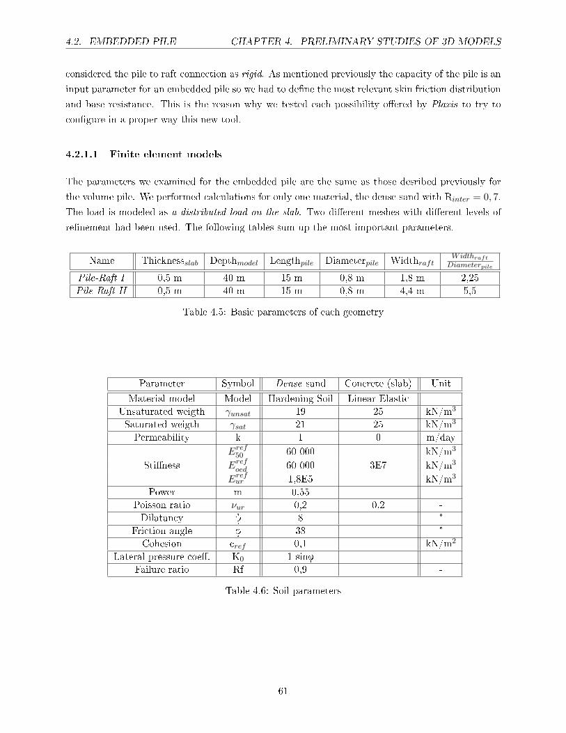
4.2 Embedded pile . . . . . . . . . . . . . . . . . . . . . . . . . . . . . . . . . . . . . . . 60
4.2.1 Embedded pile-raft . . . . . . . . . . . . . . . . . . . . . . . . . . . . . . . . . 60
4.2.1.1 Finite element models . . . . . . . . . . . . . . . . . . . . . . . . . . 61
4
CONTENTS CONTENTS
4.2.1.2 Embedded pile with linear skin friction distribution . . . . . . . . 63
4.2.1.3 Embedded pile with multilinear skin friction distribution . . . . . 69
4.2.1.4 Embedded pile with layer dependent skin friction distribution . 73
4.2.1.5 Comparison of the three options: Linear, multilinear and layer de-
pendent . . . . . . . . . . . . . . . . . . . . . . . . . . . . . . . . . . 77
5 Group e�ect 82
5.1 Presentation of calculations . . . . . . . . . . . . . . . . . . . . . . . . . . . . . . . . 82
5.1.1 Geometry . . . . . . . . . . . . . . . . . . . . . . . . . . . . . . . . . . . . . . 83
5.1.2 Finite element model . . . . . . . . . . . . . . . . . . . . . . . . . . . . . . . . 86
5.2 Results . . . . . . . . . . . . . . . . . . . . . . . . . . . . . . . . . . . . . . . . . . . . 86
5.2.1 Vocabulary details . . . . . . . . . . . . . . . . . . . . . . . . . . . . . . . . . 86
5.2.2 Load-displacement curves . . . . . . . . . . . . . . . . . . . . . . . . . . . . . 87
5.2.3 Displacement pro�les . . . . . . . . . . . . . . . . . . . . . . . . . . . . . . . . 89
5.2.4 More precise analysis of group 5 . . . . . . . . . . . . . . . . . . . . . . . . . 92
5.2.5 Conclusion . . . . . . . . . . . . . . . . . . . . . . . . . . . . . . . . . . . . . 97
6 Conclusion 98
5
Chapter 1
Introduction
In traditional foundation design, it is customary to consider �rst the use of shallow foundation such
as a raft (possibly after some ground-improvement methodology performed). If it is not adequate,
deep foundation such as a fully piled foundation is used instead. In the last few decade, an alternative
solution has been designed: piled raft foundation. Unlike the conventional piled foundation design in
which the piles are designed to carry the majority of the load, the design of a piled raft foundation
allows the load to be shared between the raft and piles and it is necessary to take the complex
soil-struture interaction e�ects into account.
The concept of piled raft foundation was �rstly proposed by Davis and Poulos in 1972 and is now
used extensively in Europe, particularly for supporting the load of high buildings or towers. The
favorable application of piled raft occurs when the raft has adequate loading capacities, but the
settlement or di�erential settlement exceed allowable values. In this case, the primary purpose of
the pile is to act as settlement reducer.
The aim of this paper is to describe a �nite element analysis of deep foundations: piled and mainly
piled raft foundations. A basic parametric study is �rstly presented to determine the in�uence of
mesh discretisation, of materials - loose or dense sand -, of dilatancy and interface elements. Then
the behavior of piled raft foundations is analysed in more details using partial axisymmetric models
of one pile-raft.
We continue by preparing a more sophisticated 3D study to take into account the complex pile-
pile interaction which occured when the pile spacing is �small�. So the possibilies of employing the
embedded pile concept as implemented into Plaxis 3D foundations is investigated. Finally, some
clues about the group e�ect are indicated.
6
Chapter 2
Preliminary studies
- 2D axisymmetric models -
In order to prepare a more sophisticated analysis a large number of calculations have been per-
formed in axisymmetric conditions. This approach o�ered the possibility to study with reasonable
calculation times the in�uence of mesh discretisation, dilatancy and interface elements for a single
pile and a pile-raft. The di�erent models and conclusions are presented in this part.
2.1 Single pile
2.1.1 Presentation of calculations
2.1.1.1 Geometry
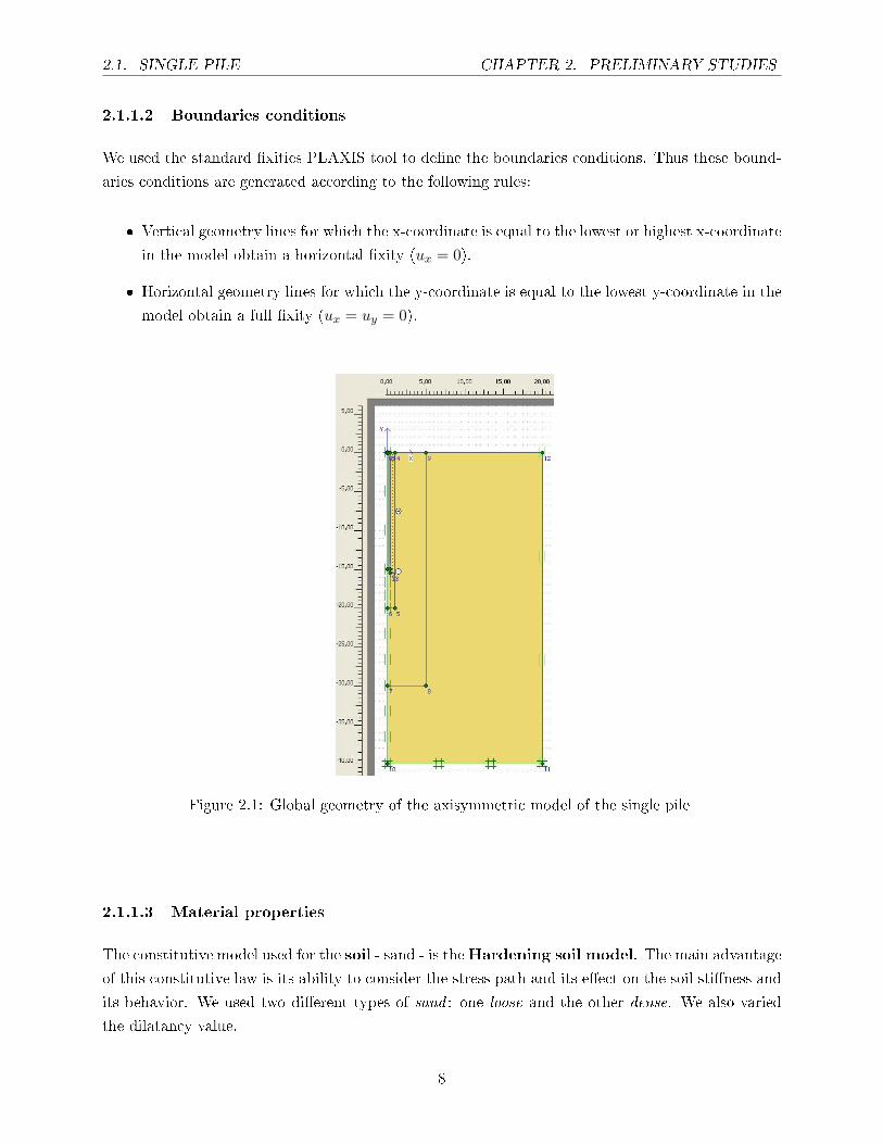
In order to analyze the behavior of the single pile, a model has been made in PLAXIS V8 using an
axisymmetric model. A working area of 20 m width and 40 m depth has been used. At the axis
of symmetry the pile has been modeled with a length of 15 m and a diameter of 0,8 m. The soil
is modeled as a single layer of sand with properties are described in 2.1.1.3). The ground water is
located at 40 m below the soil surface. In this way we did not take into account the water
in�uence. Along the length of the pile an interface has been modeled. We extended this interface
to 0,5 m below the pile inside the soil body to prevent stress oscillation in this sti� corner area.1
We added two clusters close to the pile to enrich easily the mesh in this more moving area.
1This �longer� interface will enhance the �exibility of the �nite element mesh in this area and will thus preventnon-physical stress results. However, these elements should not introduce an unrealistic weakness in the soil accordingto PLAXIS V8 manual.
7
2.1. SINGLE PILE CHAPTER 2. PRELIMINARY STUDIES
2.1.1.2 Boundaries conditions
We used the standard �xities PLAXIS tool to de�ne the boundaries conditions. Thus these bound-
aries conditions are generated according to the following rules:
� Vertical geometry lines for which the x-coordinate is equal to the lowest or highest x-coordinate
in the model obtain a horizontal �xity (ux = 0).
� Horizontal geometry lines for which the y-coordinate is equal to the lowest y-coordinate in the
model obtain a full �xity (ux = uy = 0).
Figure 2.1: Global geometry of the axisymmetric model of the single pile
2.1.1.3 Material properties
The constitutive model used for the soil - sand - is theHardening soil model. The main advantage
of this constitutive law is its ability to consider the stress path and its e�ect on the soil sti�ness and
its behavior. We used two di�erent types of sand : one loose and the other dense. We also varied
the dilatancy value.
8
2.1. SINGLE PILE CHAPTER 2. PRELIMINARY STUDIES
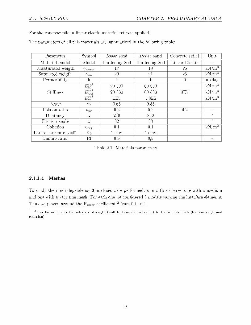
For the concrete pile, a linear elastic material set was applied.
The parameters of all this materials are summarized in the following table:
Parameter Symbol Loose sand Dense sand Concrete (pile) Unit
Material model Model Hardening Soil Hardening Soil Linear Elastic -
Unsaturated weigth γunsat 17 19 25 kN/m3
Saturated weigth γsat 20 21 25 kN/m3
Permeability k 1 1 0 m/day
Eref50 20 000 60 000 kN/m3
Sti�ness Erefoed 20 000 60 000 3E7 kN/m3
Erefur 1E5 1,8E5 kN/m3
Power m 0,65 0,55
Poisson ratio νur 0,2 0,2 0,2 -
Dilatancy y 2/0 8/0 °
Friction angle f 32 38 °
Cohesion cref 0,1 0,1 kN/m2
Lateral pressure coe�. K0 1-sinf 1-sinf -
Failure ratio Rf 0,9 0,9 -
Table 2.1: Materials parameters
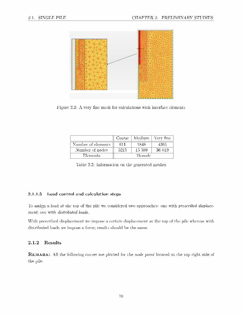
2.1.1.4 Meshes
To study the mesh dependency 3 analyses were performed: one with a coarse, one with a medium
and one with a very �ne mesh. For each one we considered 6 models varying the interface elements.
Thus we played around the Rinter coe�cient2 from 0,1 to 1.
2This factor relates the interface strength (wall friction and adhesion) to the soil strength (friction angle andcohesion)
9
2.1. SINGLE PILE CHAPTER 2. PRELIMINARY STUDIES
Figure 2.2: A very �ne mesh for calculations with interface elements
Coarse Medium Very �ne
Number of elements 611 1848 4365
Number of nodes 5215 15 389 36 019
Elements 15-node
Table 2.2: Information on the generated meshes
2.1.1.5 Load control and calculation steps
To assign a load at the top of the pile we considered two approaches: one with prescribed displace-
ment, one with distributed loads.
With prescribed displacement we impose a certain displacement at the top of the pile whereas with
distributed loads we impose a force; results should be the same.
2.1.2 Results
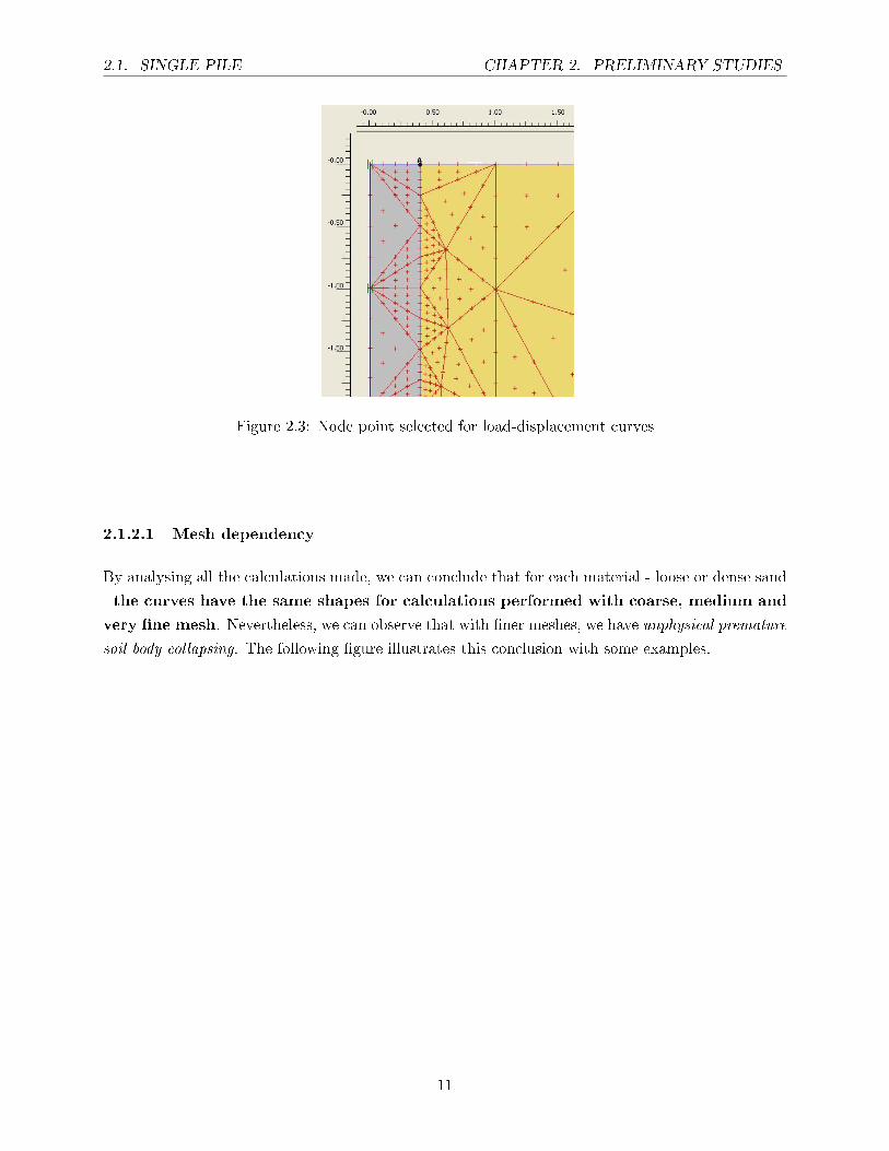
Remark: All the following curves are plotted for the node point located at the top right side of
the pile.
10
2.1. SINGLE PILE CHAPTER 2. PRELIMINARY STUDIES
Figure 2.3: Node point selected for load-displacement curves
2.1.2.1 Mesh dependency
By analysing all the calculations made, we can conclude that for each material - loose or dense sand
- the curves have the same shapes for calculations performed with coarse, medium and
very �ne mesh. Nevertheless, we can observe that with �ner meshes, we have unphysical premature
soil body collapsing. The following �gure illustrates this conclusion with some examples.
11
2.1. SINGLE PILE CHAPTER 2. PRELIMINARY STUDIES
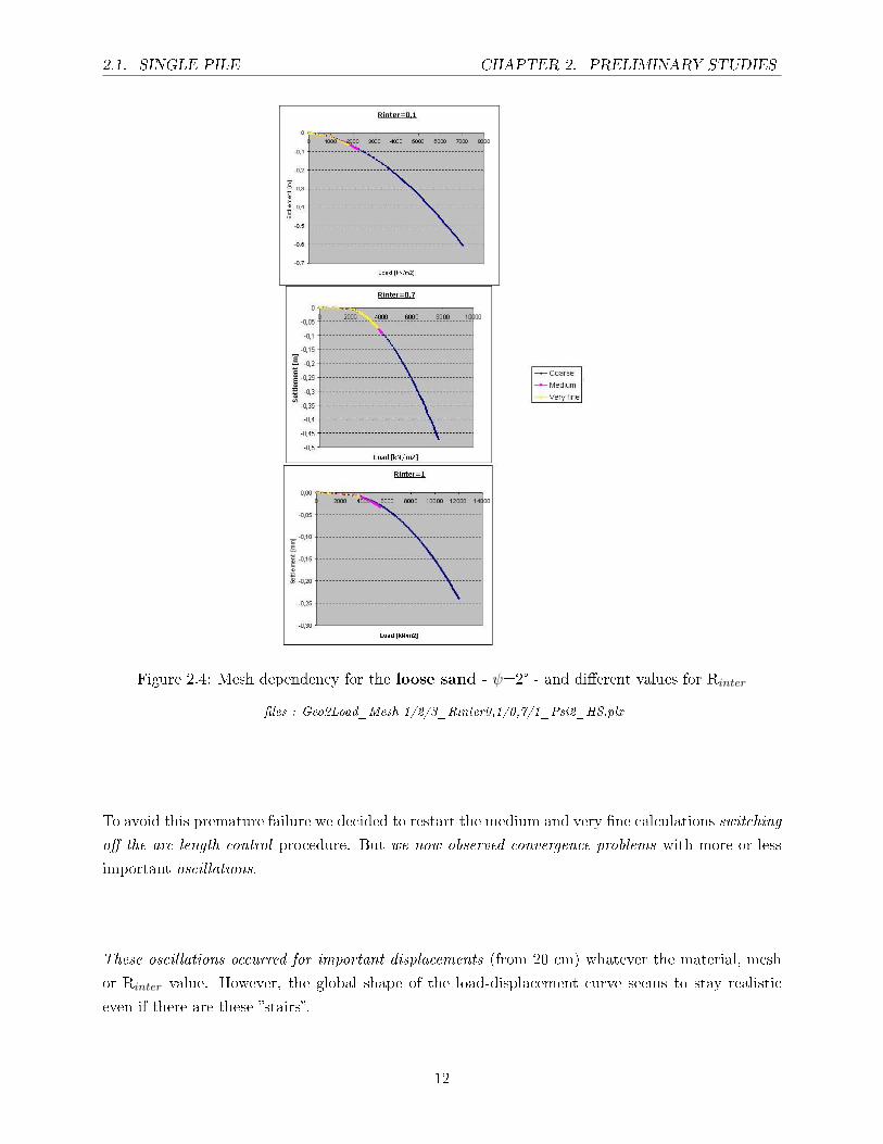
Figure 2.4: Mesh dependency for the loose sand - ψ=2° - and di�erent values for Rinter
�les : Geo2Load_Mesh 1/2/3_Rinter0,1/0,7/1_Psi2_HS.plx
To avoid this premature failure we decided to restart the medium and very �ne calculations switching
o� the arc length control procedure. But we now observed convergence problems with more or less
important oscillations.
These oscillations occurred for important displacements (from 20 cm) whatever the material, mesh
or Rinter value. However, the global shape of the load-displacement curve seems to stay realistic
even if there are these �stairs�.
12
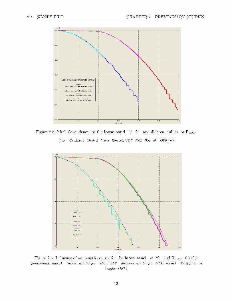
2.1. SINGLE PILE CHAPTER 2. PRELIMINARY STUDIES
Figure 2.5: Mesh dependency for the loose sand - ψ=2° - and di�erent values for Rinter
�les : Geo2Load_Mesh 2_Loose_Rinter0,1/0,7_Psi2_HS(_alc=OFF).plx
Figure 2.6: In�uence of arc length control for the loose sand - ψ=2° - and Rinter=0,7/0,1parameters: mesh1= coarse, arc length=ON; mesh2= medium, arc length=OFF; mesh3= Very �ne, arc
length=OFF;
13
2.1. SINGLE PILE CHAPTER 2. PRELIMINARY STUDIES
The �gure 2.6 enables us to con�rm that the mesh dependency is negligible for this model.
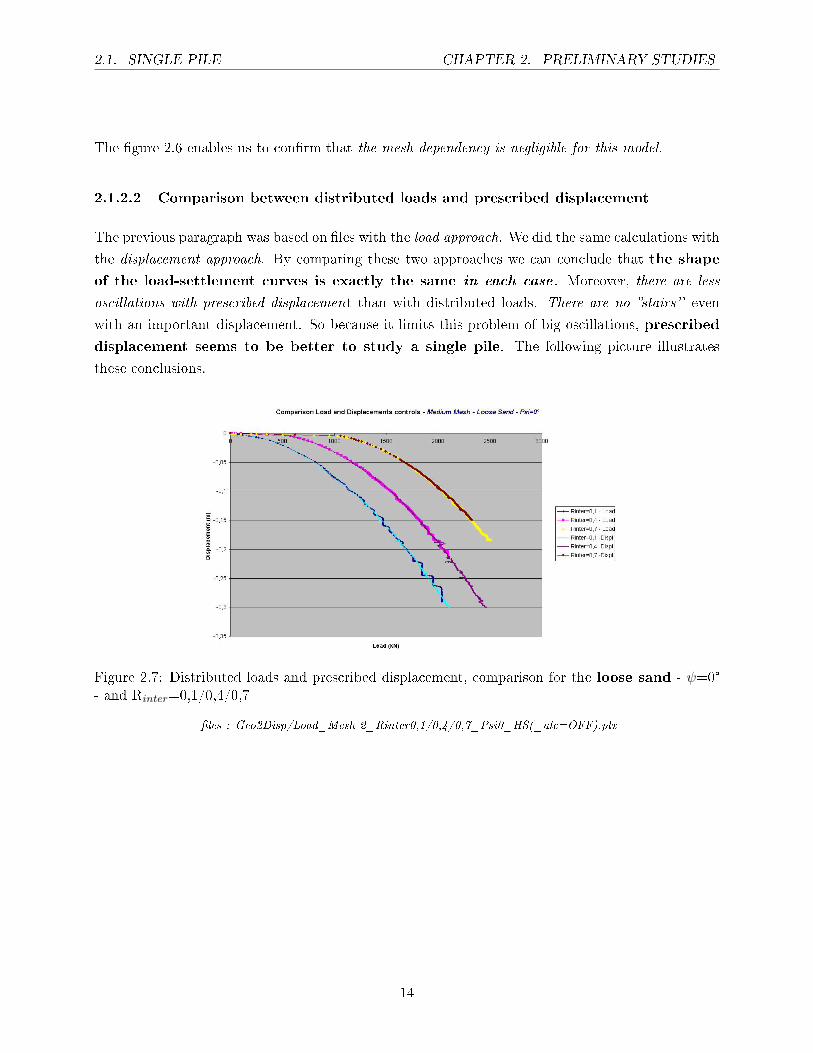
2.1.2.2 Comparison between distributed loads and prescribed displacement
The previous paragraph was based on �les with the load approach. We did the same calculations with
the displacement approach. By comparing these two approaches we can conclude that the shape
of the load-settlement curves is exactly the same in each case . Moreover, there are less
oscillations with prescribed displacement than with distributed loads. There are no �stairs' ' even
with an important displacement. So because it limits this problem of big oscillations, prescribed
displacement seems to be better to study a single pile. The following picture illustrates
these conclusions.
Figure 2.7: Distributed loads and prescribed displacement, comparison for the loose sand - ψ=0°- and Rinter=0,1/0,4/0,7
�les : Geo2Disp/Load_Mesh 2_Rinter0,1/0,4/0,7_Psi0_HS(_alc=OFF).plx
14
2.1. SINGLE PILE CHAPTER 2. PRELIMINARY STUDIES
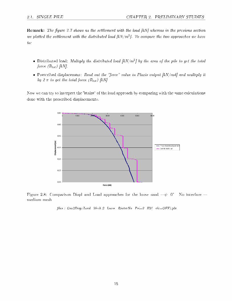
Remark: The �gure 2.7 shows us the settlement with the load [kN] whereas in the previous section
we plotted the settlement with the distributed load [kN/m2]. To compare the two approaches we have
to:
� Distributed load: Multiply the distributed load [kN/m2] by the area of the pile to get the totalforce (Rtot) [kN].
� Prescribed displacement: Read out the �force� value in Plaxis output [kN/rad] and multiply itby 2 π to get the total force (Rtot) [kN]
Now we can try to interpret the �stairs� of the load approach by comparing with the same calculations
done with the prescribed displacements.
Figure 2.8: Comparison Displ and Load approaches for the loose sand � ψ=0° - No interface �medium mesh
�les : Geo2Disp/Load_Mesh 2_Loose_RinterNo_Psi=0_HS(_alc=OFF).plx
15
2.1. SINGLE PILE CHAPTER 2. PRELIMINARY STUDIES
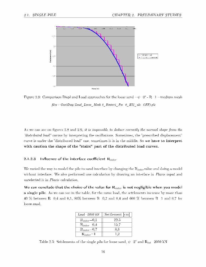
Figure 2.9: Comparison Displ and Load approaches for the loose sand � ψ=0° - R=1 � medium mesh
�les : Geo2Disp/Load_Loose_Mesh 2_Rinter1_Psi=0_HS(_alc=OFF).plx
As we can see on �gures 2.8 and 2.9, it is impossible to deduce correctly the normal shape from the
�distributed load� curves by interpreting the oscillations. Sometimes, the �prescribed displacement�
curve is under the �distributed load� one, sometimes it is in the middle. So we have to interpret
with caution the shape of the �stairs� part of the distributed load curves.
2.1.2.3 In�uence of the interface coe�cient Rinter
We varied the way to model the pile to sand interface by changing the Rintervalue and doing a model
without interface. We also performed one calculation by drawing an interface in Plaxis input and
unselected it in Plaxis calculation.
We can conclude that the choice of the value for Rinter is not negligible when you model
a single pile. As we can see in the table, for the same load, the settlements increase by more than
40 % between R=0,4 and 0,1, 80% between R=0,7 and 0,4 and 600 % between R=1 and 0,7 for
loose sand.
Load=2000 kN Settlement [cm]
Rinter=0,1 22,5
Rinter=0,4 15,7
Rinter=0,7 8,6
Rinter=1 1,2
Table 2.3: Settlements of the single pile for loose sand, ψ=2° and Rtot=2000 kN
16
2.1. SINGLE PILE CHAPTER 2. PRELIMINARY STUDIES
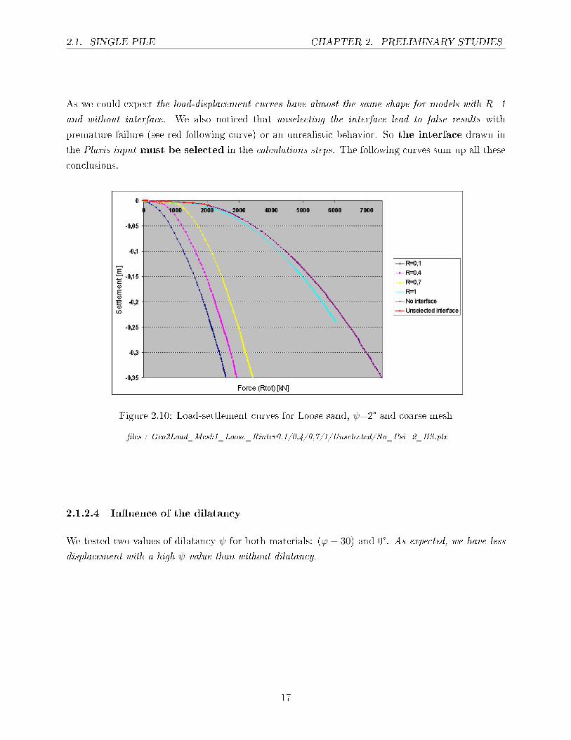
As we could expect the load-displacement curves have almost the same shape for models with R=1
and without interface. We also noticed that unselecting the interface lead to false results with
premature failure (see red following curve) or an unrealistic behavior. So the interface drawn in
the Plaxis input must be selected in the calculations steps. The following curves sum up all these
conclusions.
Figure 2.10: Load-settlement curves for Loose sand, ψ=2° and coarse mesh
�les : Geo2Load_Mesh1_Loose_Rinter0,1/0,4/0,7/1/Unselected/No_Psi=2_HS.plx
2.1.2.4 In�uence of the dilatancy
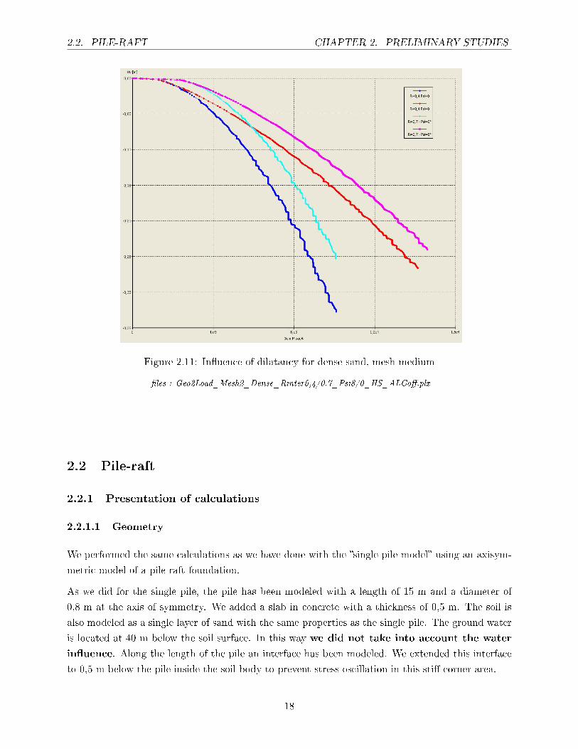
We tested two values of dilatancy ψ for both materials: (ϕ− 30) and 0°. As expected, we have less
displacement with a high ψ value than without dilatancy.
17
2.2. PILE-RAFT CHAPTER 2. PRELIMINARY STUDIES
Figure 2.11: In�uence of dilatancy for dense sand, mesh medium
�les : Geo2Load_Mesh2_Dense_Rinter0,4/0,7_Psi8/0_HS_ALCo�.plx
2.2 Pile-raft
2.2.1 Presentation of calculations
2.2.1.1 Geometry
We performed the same calculations as we have done with the �single pile model� using an axisym-
metric model of a pile-raft foundation.
As we did for the single pile, the pile has been modeled with a length of 15 m and a diameter of
0,8 m at the axis of symmetry. We added a slab in concrete with a thickness of 0,5 m. The soil is
also modeled as a single layer of sand with the same properties as the single pile. The ground water
is located at 40 m below the soil surface. In this way we did not take into account the water
in�uence. Along the length of the pile an interface has been modeled. We extended this interface
to 0,5 m below the pile inside the soil body to prevent stress oscillation in this sti� corner area.
18
2.2. PILE-RAFT CHAPTER 2. PRELIMINARY STUDIES
2.2.1.2 Boundaries conditions
We also used for this study the standard �xities PLAXIS tool (see 2.1.1.2).
2.2.1.3 Materials properties
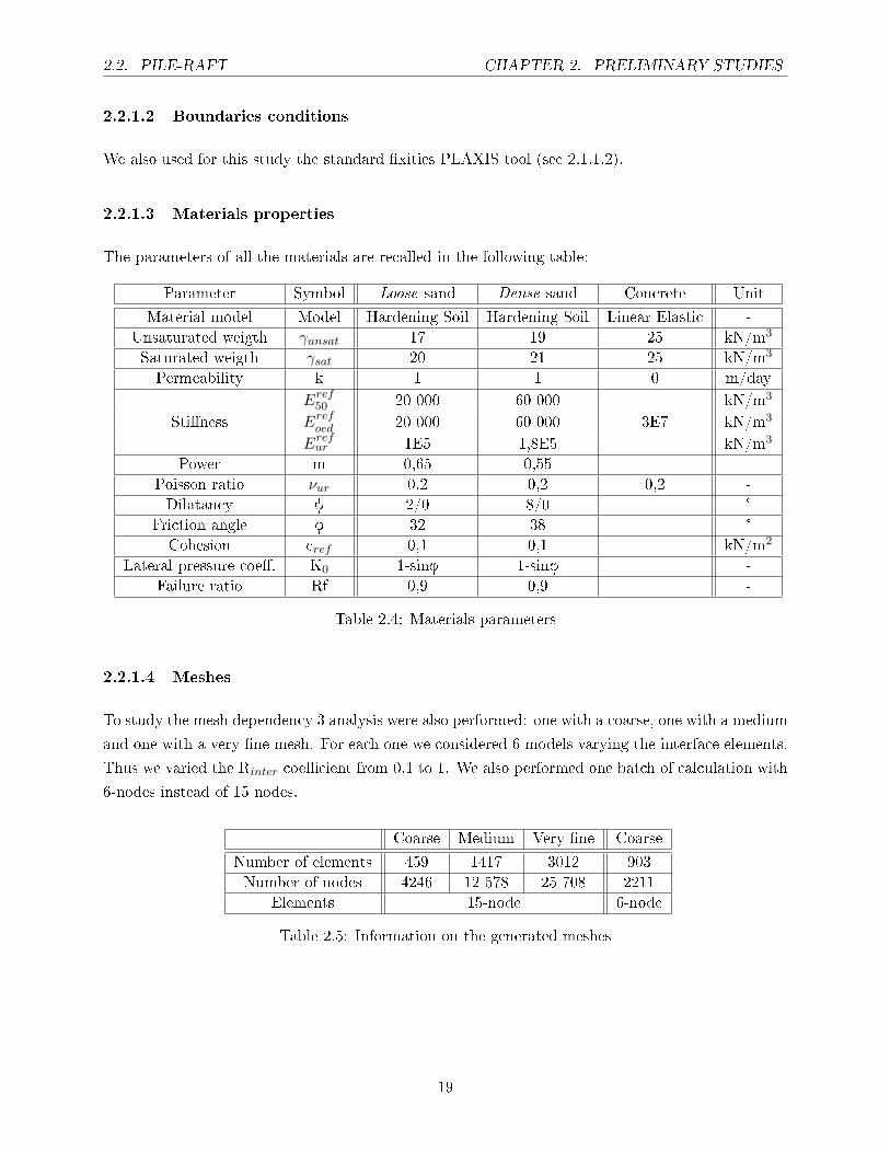
The parameters of all the materials are recalled in the following table:
Parameter Symbol Loose sand Dense sand Concrete Unit
Material model Model Hardening Soil Hardening Soil Linear Elastic -
Unsaturated weigth γunsat 17 19 25 kN/m3
Saturated weigth γsat 20 21 25 kN/m3
Permeability k 1 1 0 m/day
Eref50 20 000 60 000 kN/m3
Sti�ness Erefoed 20 000 60 000 3E7 kN/m3
Erefur 1E5 1,8E5 kN/m3
Power m 0,65 0,55
Poisson ratio νur 0,2 0,2 0,2 -
Dilatancy y 2/0 8/0 °
Friction angle f 32 38 °
Cohesion cref 0,1 0,1 kN/m2
Lateral pressure coe�. K0 1-sinf 1-sinf -
Failure ratio Rf 0,9 0,9 -
Table 2.4: Materials parameters
2.2.1.4 Meshes
To study the mesh dependency 3 analysis were also performed: one with a coarse, one with a medium
and one with a very �ne mesh. For each one we considered 6 models varying the interface elements.
Thus we varied the Rinter coe�cient from 0,1 to 1. We also performed one batch of calculation with
6-nodes instead of 15 nodes.
Coarse Medium Very �ne Coarse
Number of elements 459 1417 3012 903
Number of nodes 4246 12 578 25 708 2211
Elements 15-node 6-node
Table 2.5: Information on the generated meshes
19
2.2. PILE-RAFT CHAPTER 2. PRELIMINARY STUDIES
2.2.1.5 Load control and calculation steps
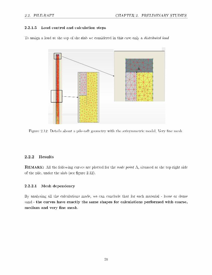
To assign a load at the top of the slab we considered in this case only a distributed load
Figure 2.12: Details about a pile-raft geometry with the axisymmetric model, Very �ne mesh
2.2.2 Results
Remark: All the following curves are plotted for the node point A, situated at the top right side
of the pile, under the slab (see �gure 2.12).
2.2.2.1 Mesh dependency
By analysing all the calculations made, we can conclude that for each material - loose or dense
sand - the curves have exactly the same shapes for calculations performed with coarse,
medium and very �ne mesh.
20
2.2. PILE-RAFT CHAPTER 2. PRELIMINARY STUDIES
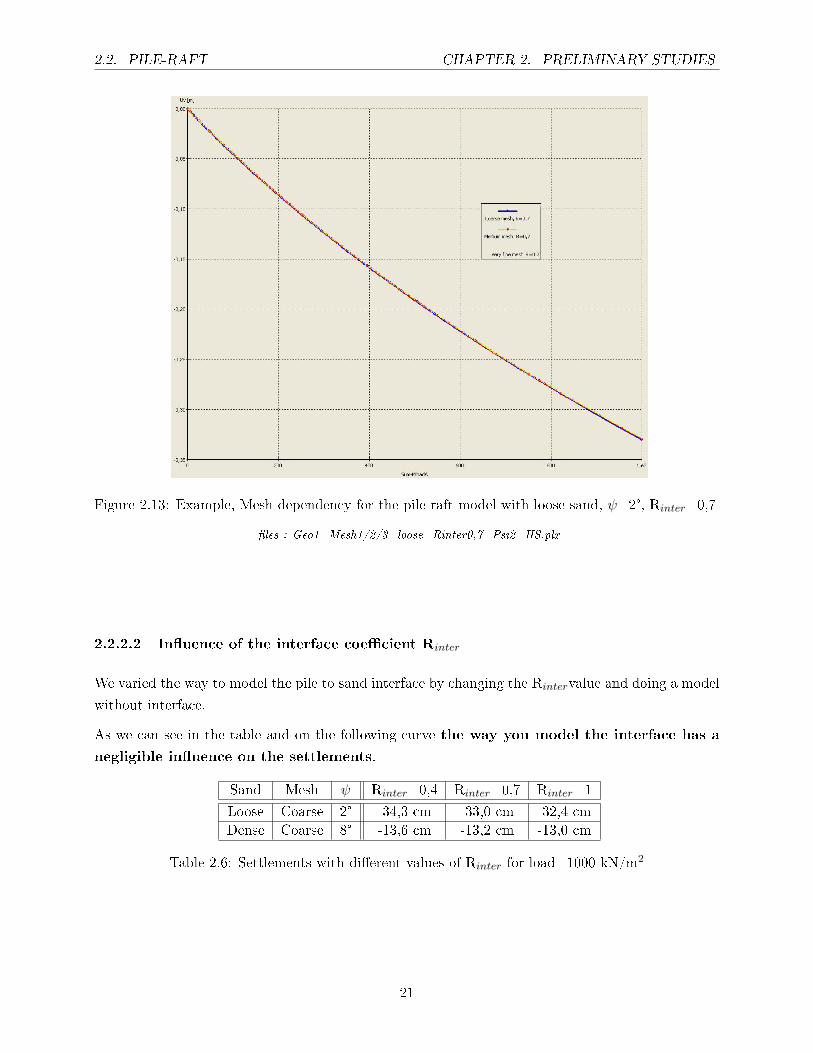
Figure 2.13: Example, Mesh dependency for the pile raft model with loose sand, ψ=2°, Rinter=0,7
�les : Geo1_Mesh1/2/3_loose_Rinter0,7_Psi2_HS.plx
2.2.2.2 In�uence of the interface coe�cient Rinter
We varied the way to model the pile to sand interface by changing the Rintervalue and doing a model
without interface.
As we can see in the table and on the following curve the way you model the interface has a
negligible in�uence on the settlements.
Sand Mesh ψ Rinter=0,4 Rinter=0,7 Rinter=1
Loose Coarse 2° -34,3 cm -33,0 cm -32,4 cm
Dense Coarse 8° -13,6 cm -13,2 cm -13,0 cm
Table 2.6: Settlements with di�erent values of Rinter for load=1000 kN/m2
21
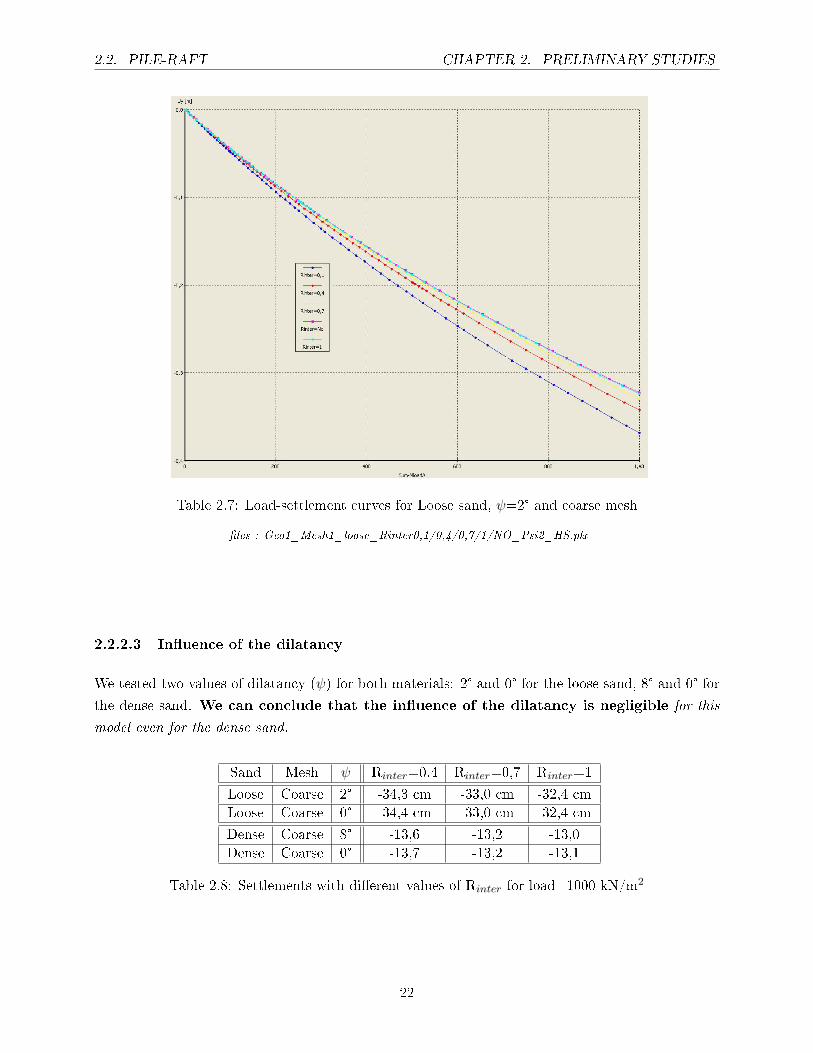
2.2. PILE-RAFT CHAPTER 2. PRELIMINARY STUDIES
Table 2.7: Load-settlement curves for Loose sand, ψ=2° and coarse mesh
�les : Geo1_Mesh1_loose_Rinter0,1/0,4/0,7/1/NO_Psi2_HS.plx
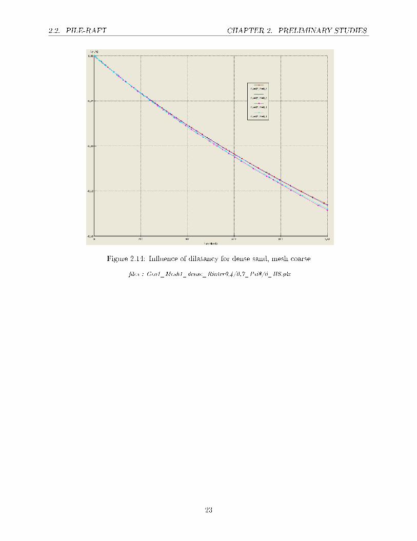
2.2.2.3 In�uence of the dilatancy
We tested two values of dilatancy (ψ) for both materials: 2° and 0° for the loose sand, 8° and 0° for
the dense sand. We can conclude that the in�uence of the dilatancy is negligible for this
model even for the dense sand.
Sand Mesh ψ Rinter=0,4 Rinter=0,7 Rinter=1
Loose Coarse 2° -34,3 cm -33,0 cm -32,4 cm
Loose Coarse 0° -34,4 cm -33,0 cm -32,4 cm
Dense Coarse 8° -13,6 -13,2 -13,0
Dense Coarse 0° -13,7 -13,2 -13,1
Table 2.8: Settlements with di�erent values of Rinter for load=1000 kN/m2
22
2.2. PILE-RAFT CHAPTER 2. PRELIMINARY STUDIES
Figure 2.14: In�uence of dilatancy for dense sand, mesh coarse
�les : Geo1_Mesh1_dense_Rinter0,4/0,7_Psi8/0_HS.plx
23
Chapter 3
Analysis of 2D models
- Behavior of a pile and a pile-raft -
In chapter 2 we made conclusions about how to de�ne e�ciently and correctly an axisymmetric
model of a single pile and a pile-raft. Now we present other calculations performed by taking these
preliminary practical conclusions into account.
In design of piled rafts, design engineers have to understand the mechanism of load transfer from
the raft to the piles and to the soil. It requires to take complex interactions into account such as:
pile-soil interaction, raft-soil interaction, pile-raft interaction and pile-pile interaction.
The aim of this chapter is to have a better understanding of the pile and raft behavior and to check
the ability of the software to model such complex interactions. In this part, we only modeled a single
pile with a raft so we did not take into account the pile-pile interaction.
3.1 Single-pile
In the previous calculations we simulated an axial load test on a bored pile. We get the following
load-displacement curve:
24
3.1. SINGLE-PILE CHAPTER 3. ANALYSIS OF 2D MODELS
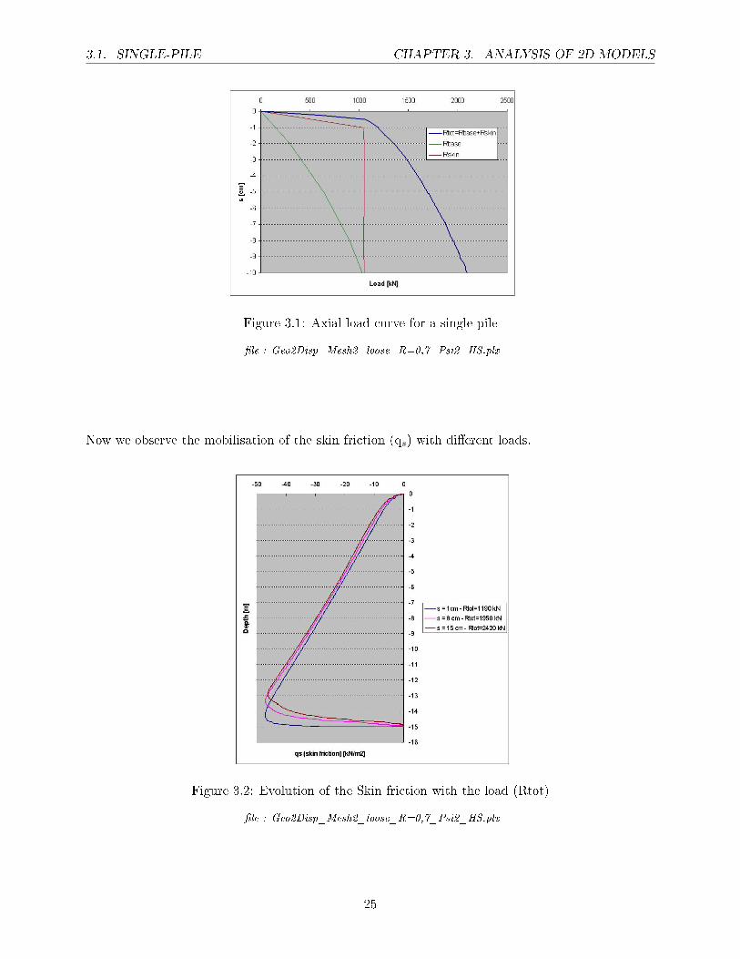
Figure 3.1: Axial load curve for a single-pile
�le : Geo2Disp_Mesh2_loose_R=0,7_Psi2_HS.plx
Now we observe the mobilisation of the skin friction (qs) with di�erent loads.
Figure 3.2: Evolution of the Skin friction with the load (Rtot)
�le : Geo2Disp_Mesh2_loose_R=0,7_Psi2_HS.plx
25
3.2. PILE-RAFT CHAPTER 3. ANALYSIS OF 2D MODELS
s = 1cm s = 8cm s = 15cmRb[kN ] 140 906 1380
Rs[kN ] 1050 1044 1040RsRb
7,5 1,15 0,75
Table 3.1: Evolution of the skin and base resistance with settlements
�le : Geo2Disp_Mesh2_loose_R=0,7_Psi2_HS.plx
That shows that the maximum skin friction is already reacted when 1,0 cm settlements occur (see
�gure 3.1). Further, the skin resistance stays the same.
3.2 Pile-Raft
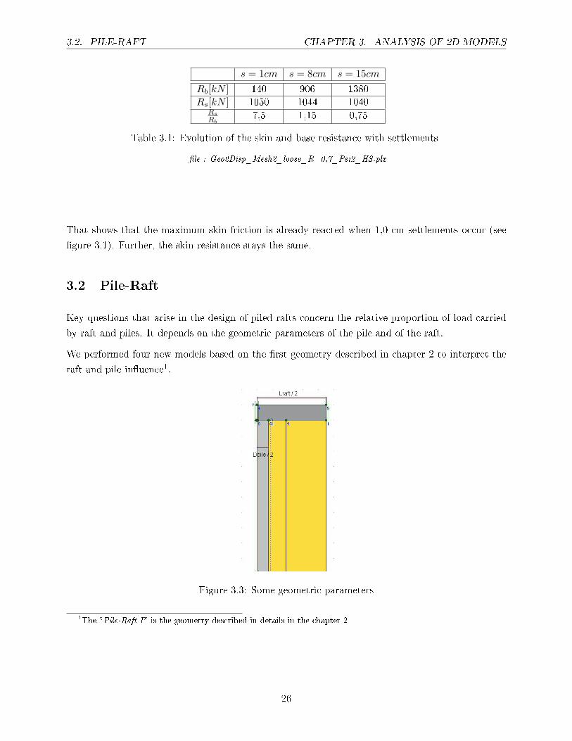
Key questions that arise in the design of piled rafts concern the relative proportion of load carried
by raft and piles. It depends on the geometric parameters of the pile and of the raft.
We performed four new models based on the �rst geometry described in chapter 2 to interpret the
raft and pile in�uence1.
Figure 3.3: Some geometric parameters
1The �Pile-Raft I � is the geometry described in details in the chapter 2
26
3.2. PILE-RAFT CHAPTER 3. ANALYSIS OF 2D MODELS
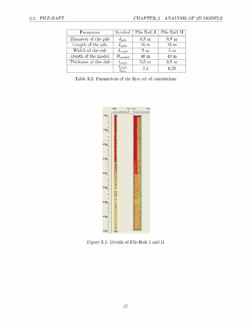
Paramater Symbol Pile-Raft I Pile-Raft II
Diameter of the pile dpile 0,8 m 0,8 m
Length of the pile Lpile 15 m 15 m
Width of the raft Lraft 2 m 5 m
Depth of the model Hmodel 40 m 40 m
Thickness of the slab traft 0,5 m 0,5 mLraft
dpile2,5 6,25
Table 3.2: Parameters of the �rst set of calculations
Figure 3.4: Details of Pile-Raft I and II
27
3.2. PILE-RAFT CHAPTER 3. ANALYSIS OF 2D MODELS
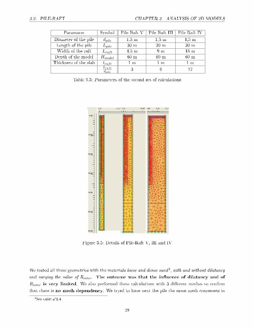
Paramater Symbol Pile-Raft V Pile-Raft III Pile-Raft IV
Diameter of the pile dpile 1,5 m 1,5 m 1,5 m
Length of the pile Lpile 30 m 30 m 30 m
Width of the raft Lraft 4,5 m 9 m 18 m
Depth of the model Hmodel 60 m 60 m 60 m
Thickness of the slab traft 1 m 1 m 1 mLraft
dpile3 6 12
Table 3.3: Parameters of the second set of calculations
Figure 3.5: Details of Pile-Raft V, III and IV
We tested all these geometries with the materials loose and dense sand2, with and without dilatancy
and varying the value of Rinter. The outcome was that the in�uence of dilatancy and of
Rinter is very limited. We also performed these calculations with 3 di�erent meshes to con�rm
that there is no mesh dependency. We tryed to have next the pile the same mesh coarseness in
2See table n°2.4
28
3.2. PILE-RAFT CHAPTER 3. ANALYSIS OF 2D MODELS
each model in order to compare precisely the di�erent models. The load is a distributed load applied
on the slab and the boundaries conditions are those described in chapter 2. In this study we did
not take into account the ground water.
Remark: As we did in chapter 2, all the load-displacement curves are plotted for the node point
A, situated at the top right side of the pile, under the slab (see �gure 2.12).
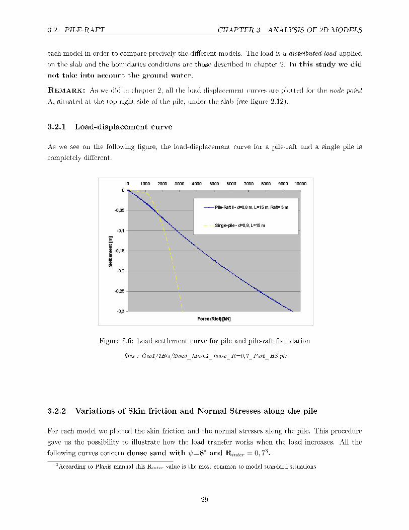
3.2.1 Load-displacement curve
As we see on the following �gure, the load-displacement curve for a pile-raft and a single pile is
completely di�erent.
Figure 3.6: Load settlement curve for pile and pile-raft foundation
�les : Geo1/1Bis/2load_Mesh1_loose_R=0,7_Psi2_HS.plx
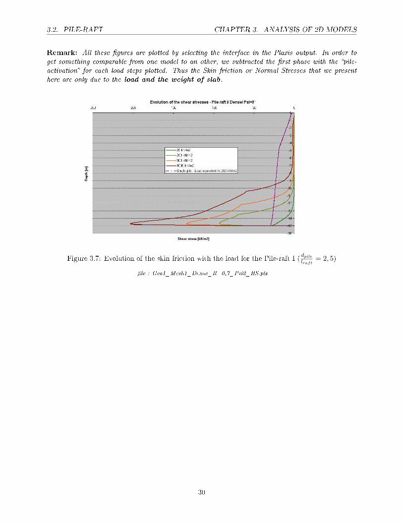
3.2.2 Variations of Skin friction and Normal Stresses along the pile
For each model we plotted the skin friction and the normal stresses along the pile. This procedure
gave us the possibility to illustrate how the load transfer works when the load increases. All the
following curves concern dense sand with ψ=8° and Rinter = 0, 73.3According to Plaxis manual this Rinter value is the most common to model standard situations
29
3.2. PILE-RAFT CHAPTER 3. ANALYSIS OF 2D MODELS
Remark: All these �gures are plotted by selecting the interface in the Plaxis output. In order toget something comparable from one model to an other, we subtracted the �rst phase with the �pile-activation� for each load steps plotted. Thus the Skin friction or Normal Stresses that we presenthere are only due to the load and the weight of slab.
Figure 3.7: Evolution of the skin friction with the load for the Pile-raft I (dpile
lraft= 2, 5)
�le : Geo1_Mesh1_Dense_R=0,7_Psi2_HS.plx
30
3.2. PILE-RAFT CHAPTER 3. ANALYSIS OF 2D MODELS
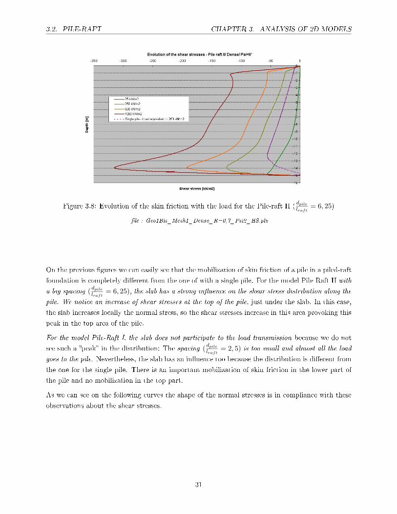
Figure 3.8: Evolution of the skin friction with the load for the Pile-raft II (dpile
lraft= 6, 25)
�le : Geo1Bis_Mesh1_Dense_R=0,7_Psi2_HS.plx
On the previous �gures we can easily see that the mobilization of skin friction of a pile in a piled-raft
foundation is completely di�erent from the one of with a single pile. For the model Pile-Raft II with
a big spacing ( dpile
lraft= 6, 25), the slab has a strong in�uence on the shear stress distribution along the
pile. We notice an increase of shear stresses at the top of the pile, just under the slab. In this case,
the slab increases locally the normal stress, so the shear stresses increase in this area provoking this
peak in the top area of the pile.
For the model Pile-Raft I, the slab does not participate to the load transmission because we do not
see such a �peak� in the distribution: The spacing ( dpile
lraft= 2, 5) is too small and almost all the load
goes to the pile. Nevertheless, the slab has an in�uence too because the distribution is di�erent from
the one for the single pile. There is an important mobilization of skin friction in the lower part of
the pile and no mobilization in the top part.
As we can see on the following curves the shape of the normal stresses is in compliance with these
observations about the shear stresses.
31
3.2. PILE-RAFT CHAPTER 3. ANALYSIS OF 2D MODELS
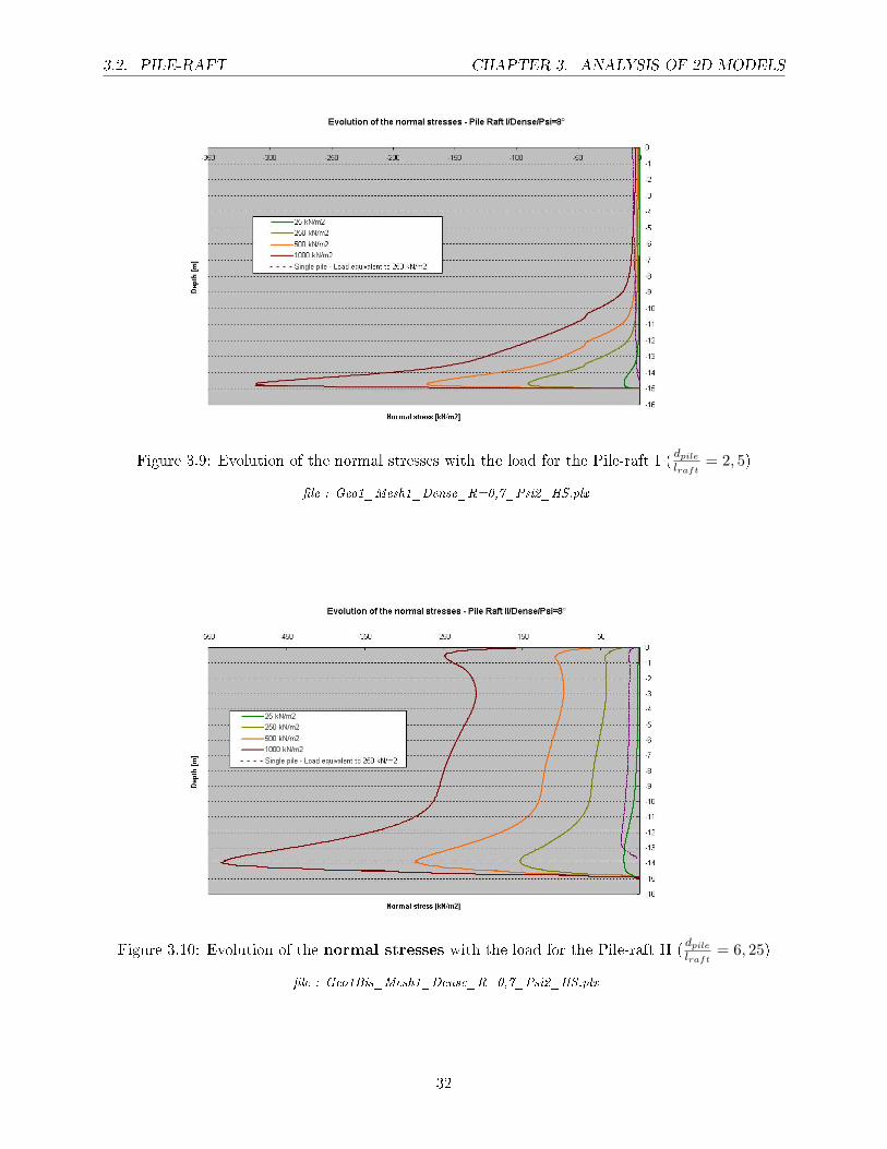
Figure 3.9: Evolution of the normal stresses with the load for the Pile-raft I (dpile
lraft= 2, 5)
�le : Geo1_Mesh1_Dense_R=0,7_Psi2_HS.plx
Figure 3.10: Evolution of the normal stresses with the load for the Pile-raft II (dpile
lraft= 6, 25)
�le : Geo1Bis_Mesh1_Dense_R=0,7_Psi2_HS.plx
32
3.2. PILE-RAFT CHAPTER 3. ANALYSIS OF 2D MODELS
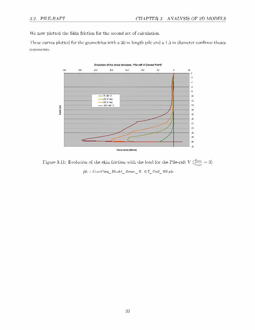
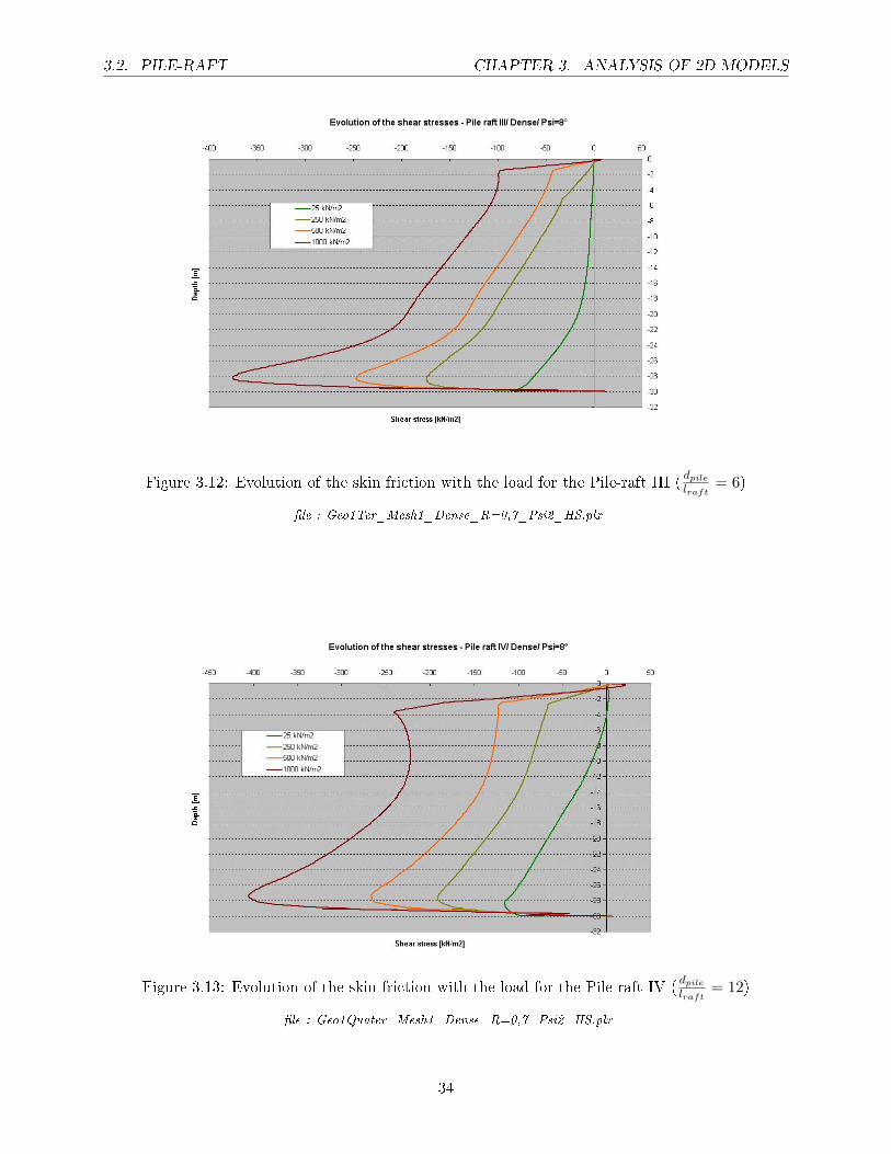
We now plotted the Skin friction for the second set of calculation.
These curves plotted for the geometries with a 30 m length pile and a 1,5 m diameter con�rme theses
comments.
Figure 3.11: Evolution of the skin friction with the load for the Pile-raft V (dpile
lraft= 3)
�le : Geo1Cinq_Mesh1_Dense_R=0,7_Psi2_HS.plx
33
3.2. PILE-RAFT CHAPTER 3. ANALYSIS OF 2D MODELS
Figure 3.12: Evolution of the skin friction with the load for the Pile-raft III (dpile
lraft= 6)
�le : Geo1Ter_Mesh1_Dense_R=0,7_Psi2_HS.plx
Figure 3.13: Evolution of the skin friction with the load for the Pile-raft IV (dpile
lraft= 12)
�le : Geo1Quater_Mesh1_Dense_R=0,7_Psi2_HS.plx
34
3.2. PILE-RAFT CHAPTER 3. ANALYSIS OF 2D MODELS
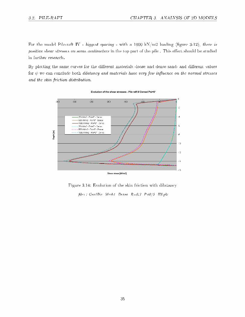
For the model Pile-raft IV - biggest spacing - with a 1000 kN/m2 loading (�gure 3-12), there is
positive shear stresses on some centimeters in the top part of the pile . This e�ect should be studied
in further research.
By plotting the same curves for the di�erent materials -loose and dense sand- and di�erent values
for ψ we can conclude both dilatancy and materials have very few in�uence on the normal stresses
and the skin friction distribution.
Figure 3.14: Evolution of the skin friction with dilatancy
�les : Geo1Bis_Mesh1_Dense_R=0,7_Psi0/8_HS.plx
35
3.2. PILE-RAFT CHAPTER 3. ANALYSIS OF 2D MODELS
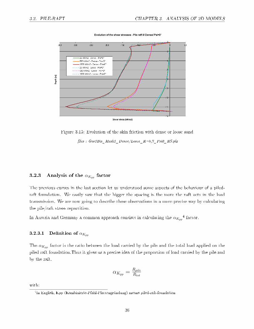
Figure 3.15: Evolution of the skin friction with dense or loose sand
�les : Geo1Bis_Mesh1_Dense/Loose_R=0,7_Psi0_HS.plx
3.2.3 Analysis of the αKpp factor
The previous curves in the last section let us understood some aspects of the behaviour of a piled-
raft foundation. We easily saw that the bigger the spacing is the more the raft acts in the load
transmission. We are now going to describe these observations in a more precise way by calculating
the pile/raft stress repartition.
In Austria and Germany a common approach consists in calculating the αKpp4 factor.
3.2.3.1 De�nition of αKpp
The αKpp factor is the ratio between the load carried by the pile and the total load applied on the
piled raft foundation.Thus it gives us a precise idea of the proportion of load carried by the pile and
by the raft.
αKpp=
Rpile
Rtot
with:
4In English, Kpp (Kombinierte-Pfahl-Plattengründung) means piled-raft-foundation
36
3.2. PILE-RAFT CHAPTER 3. ANALYSIS OF 2D MODELS
� Rpile = Rb +Rs = Load carried by the pile 5 [kN]
� Rtot =Total load =Distributed load on the slab + weigth of the slab = Rraft +Rpile6 [kN]
So it means that:
� If αKpp = 1 , all the load is carried by the pile
� If αKpp = 0 , all the load is carried by the raft
We will also use the (1-αKpp) coe�cient which represents the proportion of load carried by the raft.
(1-αKpp)=
Rraft
Rtot
Remark: Again the weight of the pile is not taken into account.
3.2.3.2 Methodology to calculate αKpp
The simplest way to calculate αKpp with Plaxis 2D consists in realizing a cross section under the
slab and reading out the normal stresses on this cross section. Then we just have to sort the normal
stresses which are into the pile and into the soil.
Remarks:
In order to get an accurate value for αKpp we need to take care of:
� Making a cross section which crosses as much stress points as possible because the value is
obtained from extrapolation.
� Making a cross section not too close to the slab because the junction Slab/pile is a high stress
variation area and singularities could occur (take 10 cm to 20 cm under the slab usually leads
to accurate values).
The following example explains in detail this methodology.
5Rb =Base resistance of the pile [kN]; Rs =Skin resistance of the pile [kN]6Rraft =Load carried by the raft [kN]
37
3.2. PILE-RAFT CHAPTER 3. ANALYSIS OF 2D MODELS
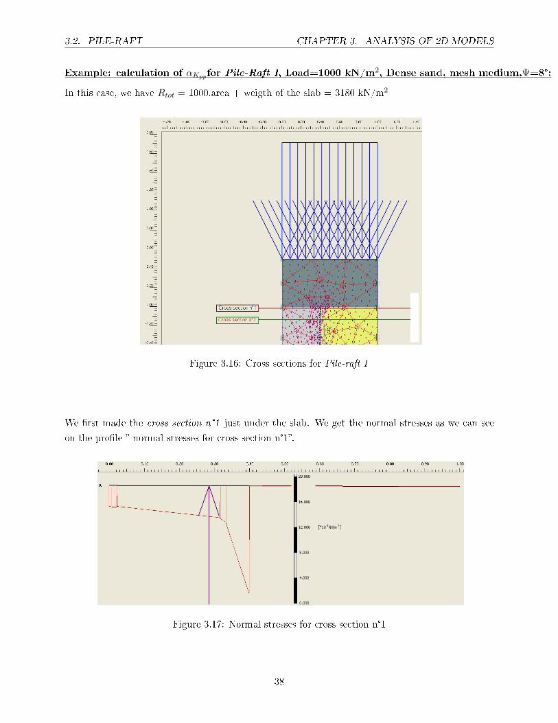
Example: calculation of αKppfor Pile-Raft I, Load=1000 kN/m2, Dense sand, mesh medium,Ψ=8°:
In this case, we have Rtot = 1000.area + weigth of the slab = 3180 kN/m2
Figure 3.16: Cross sections for Pile-raft I
We �rst made the cross section n°1 just under the slab. We get the normal stresses as we can see
on the pro�le � normal stresses for cross section n°1�.
Figure 3.17: Normal stresses for cross section n°1
38
3.2. PILE-RAFT CHAPTER 3. ANALYSIS OF 2D MODELS
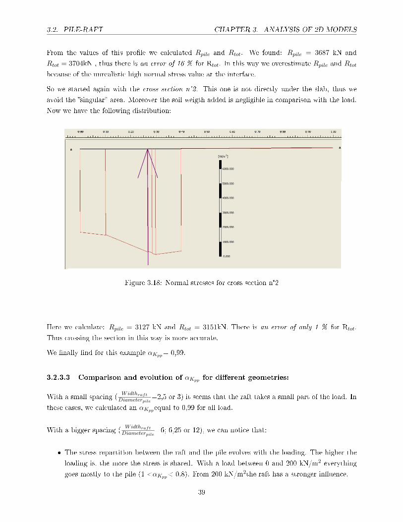
From the values of this pro�le we calculated Rpile and Rtot. We found: Rpile = 3687 kN and
Rtot = 3704kN , thus there is an error of 16 % for Rtot. In this way we overestimate Rpile and Rtot
because of the unrealistic high normal stress value at the interface.
So we started again with the cross section n°2. This one is not directly under the slab, thus we
avoid the �singular� area. Moreover the soil weigth added is negligible in comparison with the load.
Now we have the following distribution:
Figure 3.18: Normal stresses for cross section n°2
Here we calculate: Rpile = 3127 kN and Rtot = 3151kN. There is an error of only 1 % for Rtot.
Thus crossing the section in this way is more accurate.
We �nally �nd for this example αKpp= 0,99.
3.2.3.3 Comparison and evolution of αKpp for di�erent geometries:
With a small spacing (Widthraft
Diameterpile=2,5 or 3) it seems that the raft takes a small part of the load. In
these cases, we calculated an αKppequal to 0,99 for all load.
With a bigger spacing (Widthraft
Diameterpile=6; 6,25 or 12), we can notice that:
� The stress repartition between the raft and the pile evolves with the loading. The higher the
loading is, the more the stress is shared. With a load between 0 and 200 kN/m2 everything
goes mostly to the pile (1 <αKpp< 0,8). From 200 kN/m2the raft has a stronger in�uence.
39
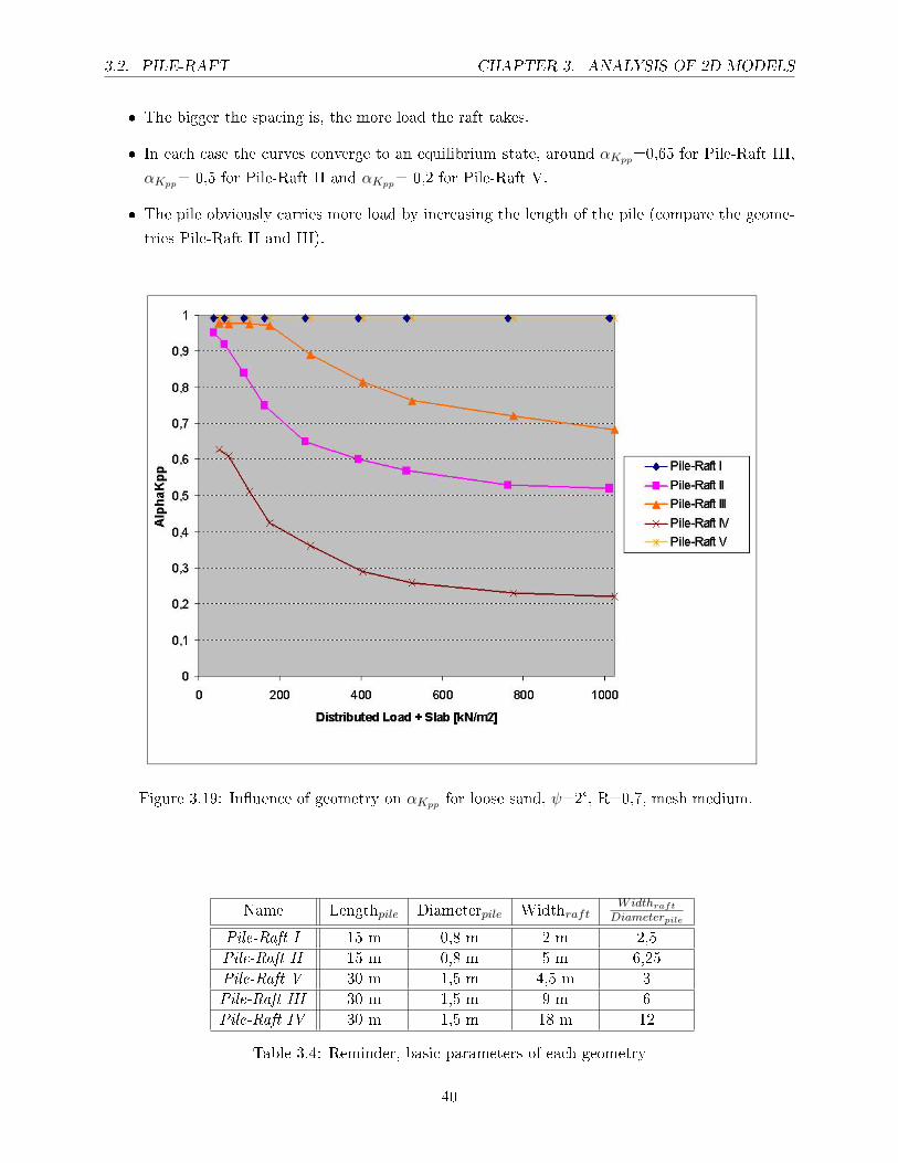
3.2. PILE-RAFT CHAPTER 3. ANALYSIS OF 2D MODELS
� The bigger the spacing is, the more load the raft takes.
� In each case the curves converge to an equilibrium state, around αKpp=0,65 for Pile-Raft III,
αKpp= 0,5 for Pile-Raft II and αKpp= 0,2 for Pile-Raft V.
� The pile obviously carries more load by increasing the length of the pile (compare the geome-
tries Pile-Raft II and III).
Figure 3.19: In�uence of geometry on αKpp for loose sand, ψ=2°, R=0,7, mesh medium.
Name Lengthpile Diameterpile WidthraftWidthraft
Diameterpile
Pile-Raft I 15 m 0,8 m 2 m 2,5
Pile-Raft II 15 m 0,8 m 5 m 6,25
Pile-Raft V 30 m 1,5 m 4,5 m 3
Pile-Raft III 30 m 1,5 m 9 m 6
Pile-Raft IV 30 m 1,5 m 18 m 12
Table 3.4: Reminder, basic parameters of each geometry
40
3.2. PILE-RAFT CHAPTER 3. ANALYSIS OF 2D MODELS
Rtot [kN/m2] 25 + Slab 250 + Slab 500 + Slab 1000 + Slab
Pile-Raft I 0,99 0,99 0,99 0,99
Pile-Raft II 0,95 0,65 0,57 0,52
Pile-Raft V 0,99 0,99 0,99 0,99
Pile-Raft III 0,96 0,85 0,71 0,62
Pile-Raft IV 0,66 0,29 0,22 0,19
Table 3.5: Few values of αKpp for loose sand, ψ=2°, R=0,7
3.2.3.4 Evolution of αKpp for di�erent materials and dilatancy
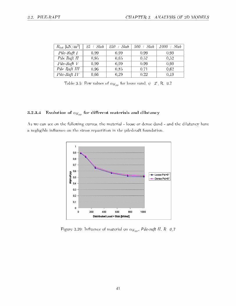
As we can see on the following curves, the material - loose or dense dand - and the dilatancy have
a negligible in�uence on the stress repartition in the piled-raft foundation.
Figure 3.20: In�uence of material on αKpp , Pile-raft II, R=0,7
41
3.2. PILE-RAFT CHAPTER 3. ANALYSIS OF 2D MODELS
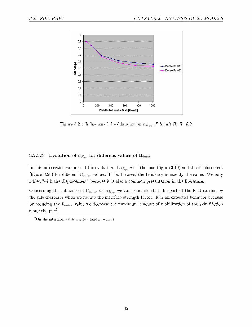
Figure 3.21: In�uence of the dilatancy on αKpp , Pile-raft II, R=0,7
3.2.3.5 Evolution of αKpp for di�erent values of Rinter
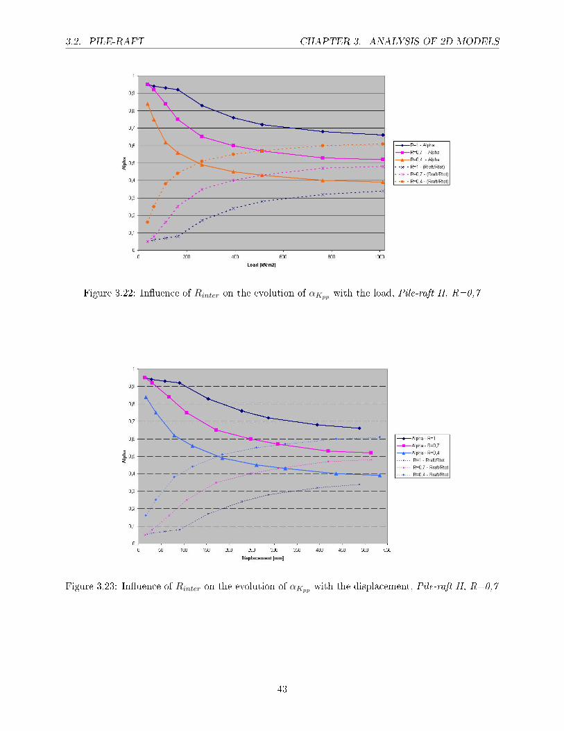
In this sub-section we present the evolution of αKpp with the load (�gure 3.19) and the displacement
(�gure 3.20) for di�erent Rinter values. In both cases, the tendency is exactly the same. We only
added �with the displacement� because it is also a common presentation in the literature.
Concerning the in�uence of Rinter on αKpp we can conclude that the part of the load carried by
the pile decreases when we reduce the interface strength factor. It is an expected behavior because
by reducing the Rinter value we decrease the maximum amount of mobilization of the skin friction
along the pile7.
7On the interface, τ≤ Rinter.(σn.tanφsoil+csoil)
42
3.2. PILE-RAFT CHAPTER 3. ANALYSIS OF 2D MODELS
Figure 3.22: In�uence of Rinter on the evolution of αKpp with the load, Pile-raft II, R=0,7
Figure 3.23: In�uence of Rinter on the evolution of αKpp with the displacement, Pile-raft II, R=0,7
43
3.2. PILE-RAFT CHAPTER 3. ANALYSIS OF 2D MODELS
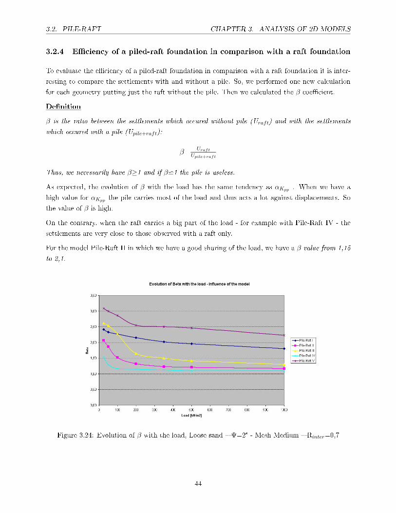
3.2.4 E�ciency of a piled-raft foundation in comparison with a raft foundation
To evaluate the e�ciency of a piled-raft foundation in comparison with a raft foundation it is inter-
resting to compare the settlements with and without a pile. So, we performed one new calculation
for each geometry putting just the raft without the pile. Then we calculated the β coe�cient.
De�nition
β is the ratio between the settlements which occured without pile (Uraft) and with the settlements
which occured with a pile (Upile+raft):
β=Uraft
Upile+raft
Thus, we necessarily have β≥1 and if βw1 the pile is useless.
As expected, the evolution of β with the load has the same tendency as αKpp . When we have a
high value for αKpp the pile carries most of the load and thus acts a lot against displacements. So
the value of β is high.
On the contrary, when the raft carries a big part of the load - for example with Pile-Raft IV - the
settlements are very close to those observed with a raft only.
For the model Pile-Raft II in which we have a good sharing of the load, we have a β value from 1,15
to 2,1.
Figure 3.24: Evolution of β with the load, Loose sand � Ψ=2° - Mesh Medium � Rinter=0,7
44
3.2. PILE-RAFT CHAPTER 3. ANALYSIS OF 2D MODELS
Rtot [kN/m2] 25 200 500 1000
Pile-Raft I 2,4 2,15 2,0 1,8
Pile-Raft II 2,1 1,3 1,2 1,15
Pile-Raft V 3,1 2,5 2,5 2,2
Pile-Raft III 2,6 1,65 1,4 1,3
Pile-Raft IV 1,5 1,15 1,1 1,0
Table 3.6: Few values of β for loose sand, ψ=2°, R=0,7
Figure 3.25: Comparison between the evolution of β and α for Pile-Raft II, loose, ψ=2°, R=0,7
3.2.5 Analysis of the pile behavior
The bearing capacity of a pile consists of the base resistance (Rb) and the skin resistance (Rs). Now
we study in detail these two forces in order to have a better idea of the pile behavior for di�erent
geometries.
3.2.5.1 Base resistance
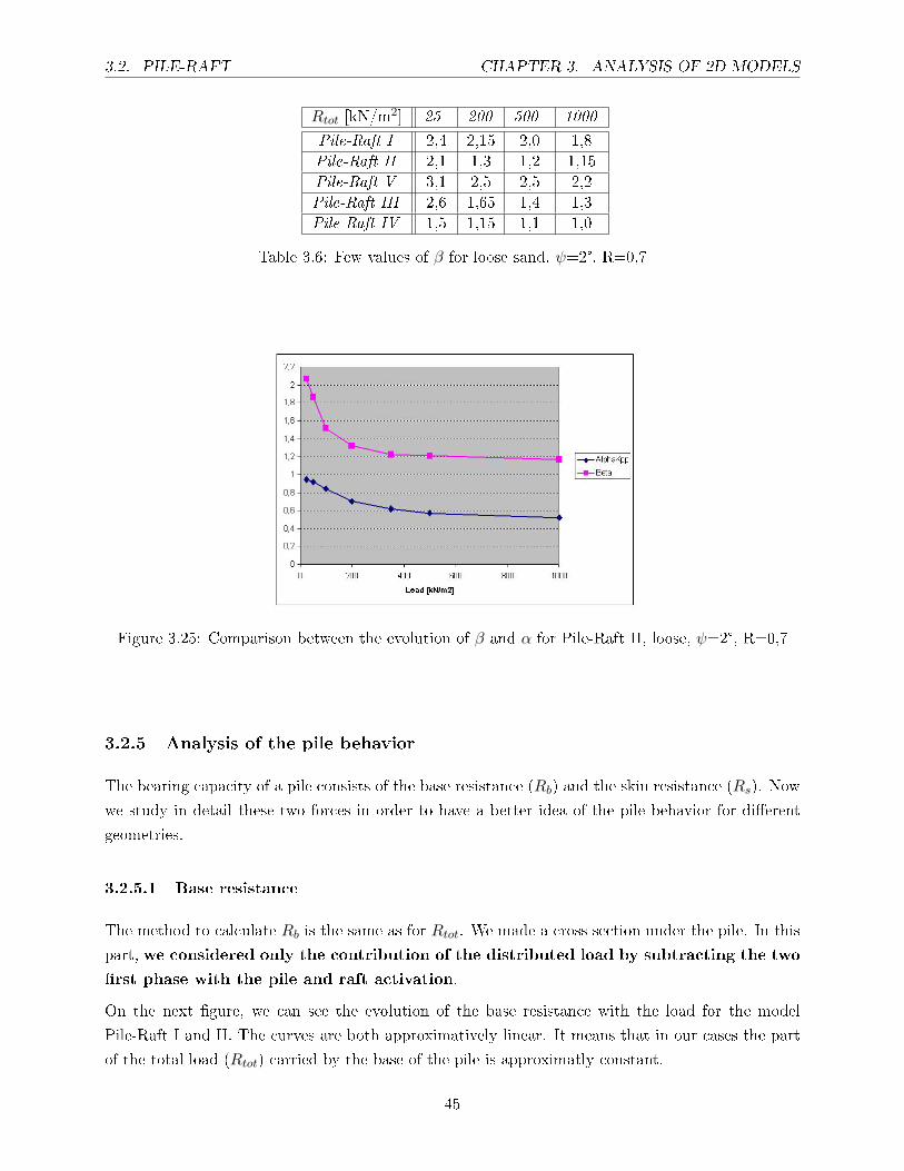
The method to calculate Rb is the same as for Rtot. We made a cross section under the pile. In this
part, we considered only the contribution of the distributed load by subtracting the two
�rst phase with the pile and raft activation.
On the next �gure, we can see the evolution of the base resistance with the load for the model
Pile-Raft I and II. The curves are both approximatively linear. It means that in our cases the part
of the total load (Rtot) carried by the base of the pile is approximatly constant.
45
3.2. PILE-RAFT CHAPTER 3. ANALYSIS OF 2D MODELS
Figure 3.26: Evolution of Rbwith the load for Pile-Raft I and II, dense sand, ψ=8°
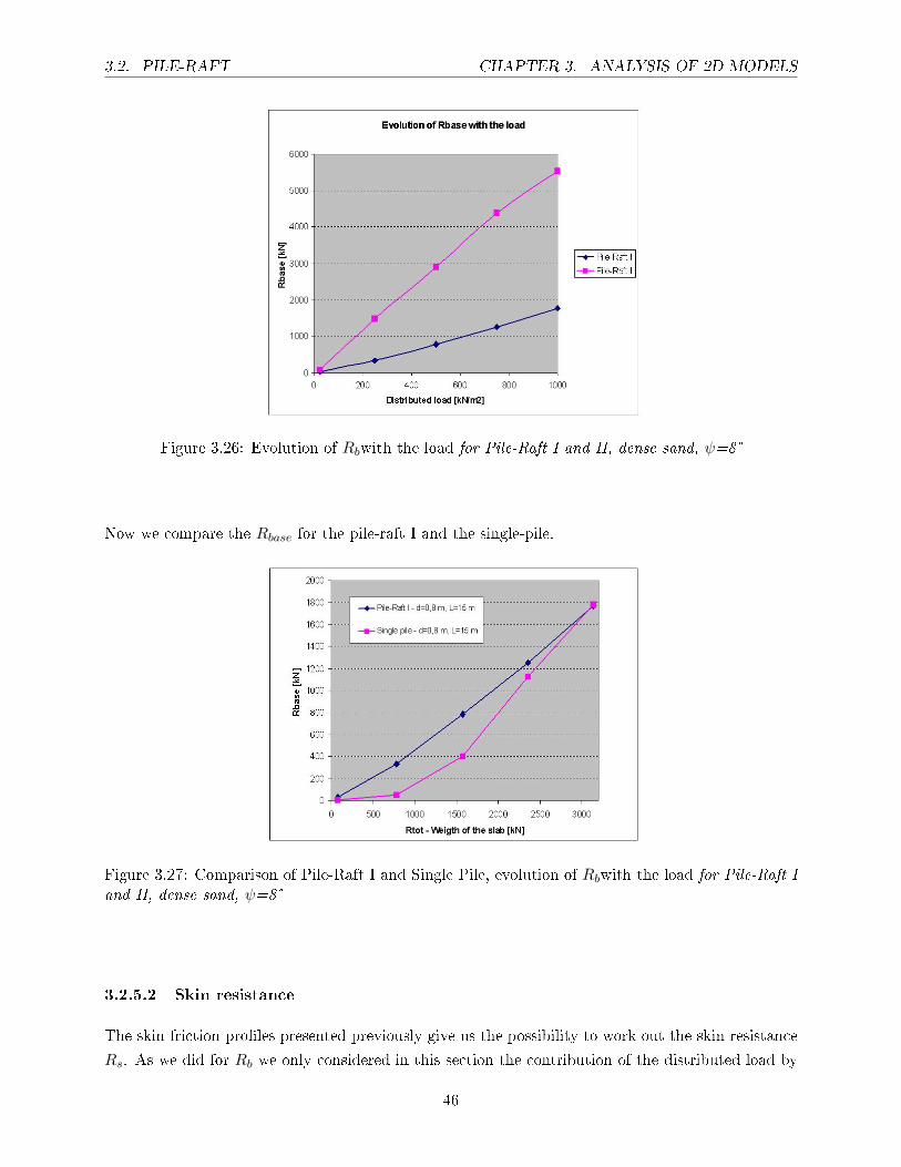
Now we compare the Rbase for the pile-raft I and the single-pile.
Figure 3.27: Comparison of Pile-Raft I and Single Pile, evolution of Rbwith the load for Pile-Raft Iand II, dense sand, ψ=8°
3.2.5.2 Skin resistance
The skin friction pro�les presented previously give us the possibility to work out the skin resistance
Rs. As we did for Rb we only considered in this section the contribution of the distributed load by
46
3.2. PILE-RAFT CHAPTER 3. ANALYSIS OF 2D MODELS
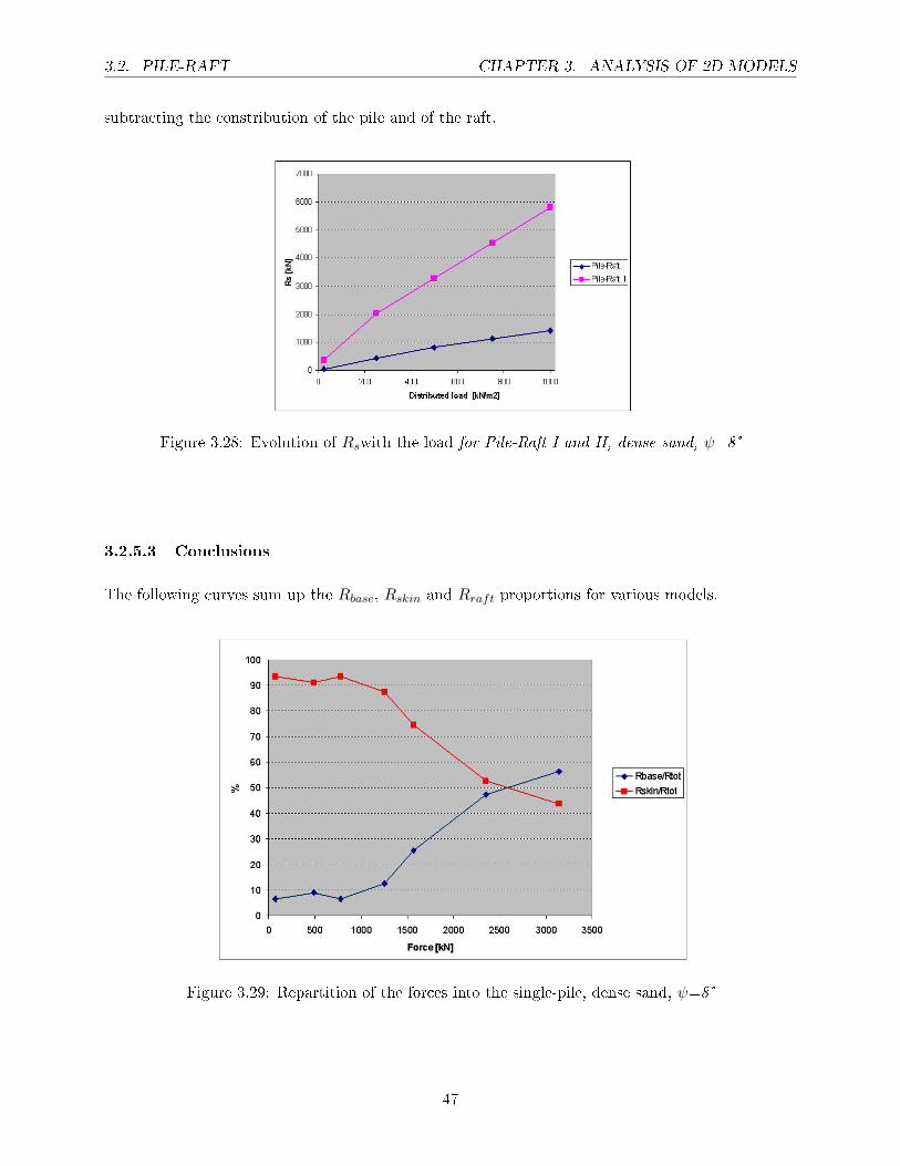
subtracting the constribution of the pile and of the raft.
Figure 3.28: Evolution of Rswith the load for Pile-Raft I and II, dense sand, ψ=8°
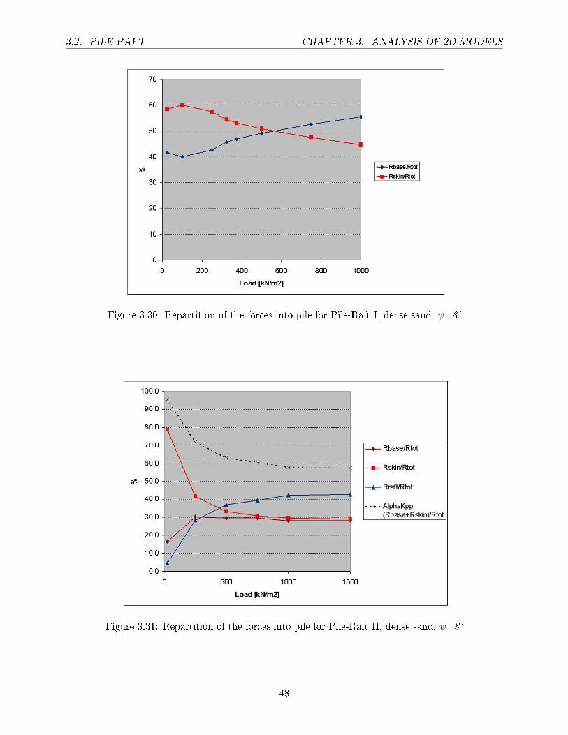
3.2.5.3 Conclusions
The following curves sum up the Rbase, Rskin and Rraft proportions for various models.
Figure 3.29: Repartition of the forces into the single-pile, dense sand, ψ=8°
47
3.2. PILE-RAFT CHAPTER 3. ANALYSIS OF 2D MODELS
Figure 3.30: Repartition of the forces into pile for Pile-Raft I, dense sand, ψ=8°
Figure 3.31: Repartition of the forces into pile for Pile-Raft II, dense sand, ψ=8°
48
Chapter 4
Preliminary studies of 3D models
- From 2D axisymmetric models to 3D models -
We previously studied the behavior of one pile-raft foundation. Nevertheless the load settlement
behavior of piles in a pile group is usually observed to be totally di�erent from the behavior of
a corresponding single pile. This group e�ect cannot be studied with axisymmetric models and
consequently it requires performing calculations with Plaxis 3D foundation.
In order to prepare the group e�ect analysis, we �rstly tested the di�erent Plaxis 3D foundation
tools to model a pile: the volume pile and a new feature, the embedded pile. These comparisons are
presented in this chapter.
Remark about the mesh dependency:
The previous calculations with axisymmetric models showed a negligible mesh dependency. We also
checked that 6-node coarse meshes lead to the same load-displacement behavior as 15-node �ne
meshes.
Due to the bigger size of working areas in 3D models we cannot use e�ciently �ne meshes. Thus,
we will perform calculations from coarse to medium meshes. The results should be realistic because
of the low sensitivity of the mesh re�nement observed in 2D.
Remark about the mesh generation:
To create a mesh with Plaxis 3D foundation we �rstly generate a 2D mesh on a horizontal work
plane. When the 2D mesh is satisfactory, the 3D mesh is generated from the 2D mesh. Since
there is no vertical re�nement option, badly shaped elements with a higher vertical than horizontal
dimension could occur. To get a satisfactory vertical re�nement, we added multiple work planes in
the input, then when the 3D mesh is generated from the 2D one, these additional planes are taken
into account and the vertical size of the elements is adapted from their spacing. In this way we get a
good medium 3D mesh with a local 3D re�nement under the slab and at the pile bottom (see �gure
4.1).
49
4.1. VOLUME PILE CHAPTER 4. PRELIMINARY STUDIES OF 3D MODELS
4.1 Volume pile
The volume pile is a common Plaxis 3D foundation option to model a pile.
4.1.1 Finite element models
To start this study, all the previous geometries (Pile-Raft I, II, III, IV, V) were modeled using Plaxis
3D foundation. The working area was adapted in each case to have the same raft area with 3D and
with axisymmetric models.
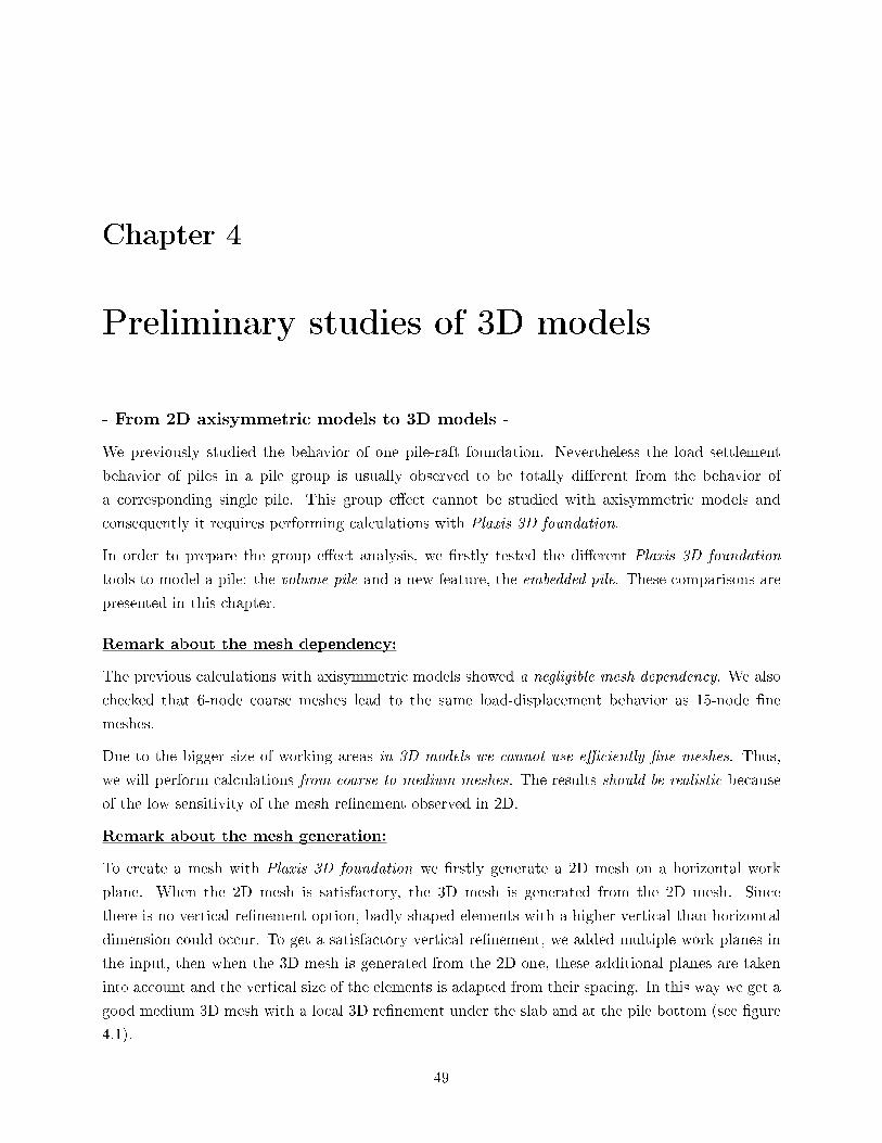
Actually the raft area with axisymmetric models is circular whereas it is a square raft in 3D. Thus
in 2D, the raft area is given by the following formula:
Araft2D= π × (
Lraft2D2 )2 [m2]
The 3D width raft is obtained by taking the square root of 2D area raft as followed:
Lraft3D=
√Araft2D
=√π × (
Lraft2D2 )2 [m]
In this way, the area of the 3D raft is equal to the one in 2D: Araft3D= Araft2D
[m2]
Figure 4.1: Comparison between the axisymmetric and 3D raft shapes
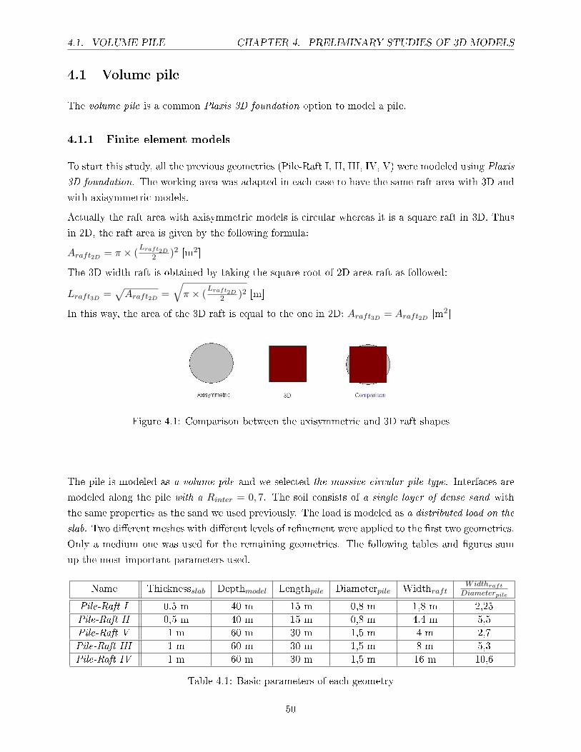
The pile is modeled as a volume pile and we selected the massive circular pile type. Interfaces are
modeled along the pile with a Rinter = 0, 7. The soil consists of a single layer of dense sand with
the same properties as the sand we used previously. The load is modeled as a distributed load on the
slab. Two di�erent meshes with di�erent levels of re�nement were applied to the �rst two geometries.
Only a medium one was used for the remaining geometries. The following tables and �gures sum
up the most important parameters used.
Name Thicknessslab Depthmodel Lengthpile Diameterpile WidthraftWidthraft
Diameterpile
Pile-Raft I 0,5 m 40 m 15 m 0,8 m 1,8 m 2,25
Pile-Raft II 0,5 m 40 m 15 m 0,8 m 4,4 m 5,5
Pile-Raft V 1 m 60 m 30 m 1,5 m 4 m 2,7
Pile-Raft III 1 m 60 m 30 m 1,5 m 8 m 5,3
Pile-Raft IV 1 m 60 m 30 m 1,5 m 16 m 10,6
Table 4.1: Basic parameters of each geometry
50
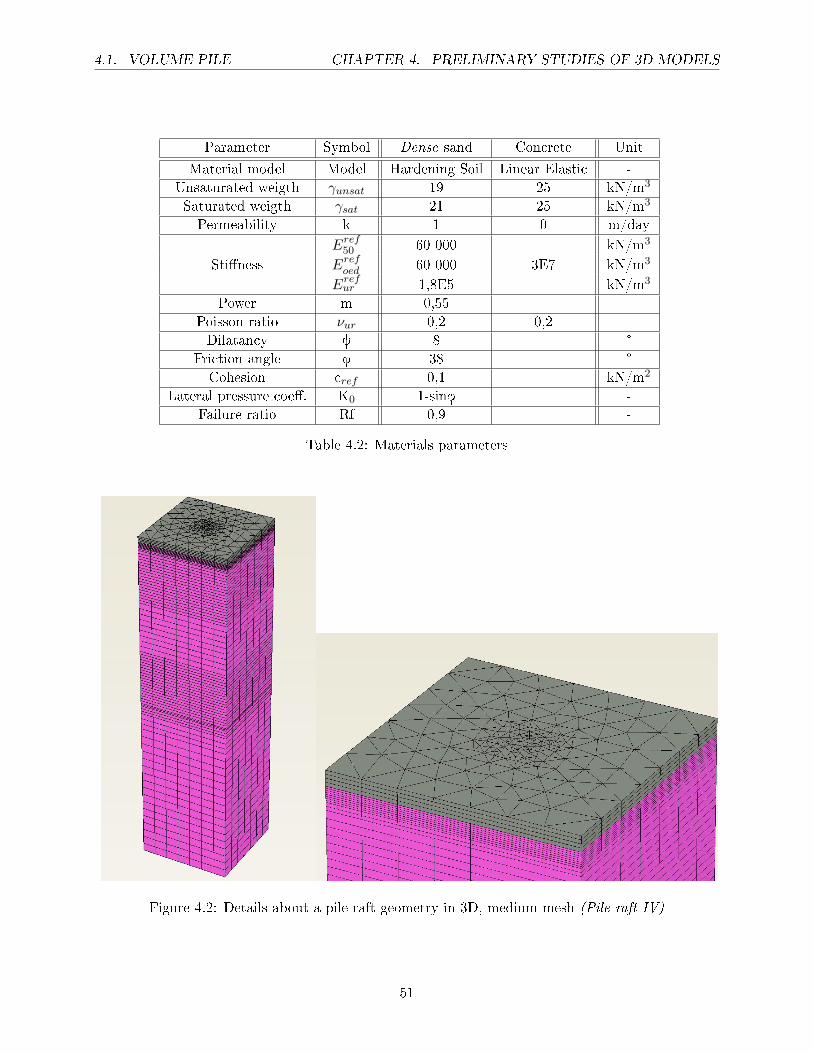
4.1. VOLUME PILE CHAPTER 4. PRELIMINARY STUDIES OF 3D MODELS
Parameter Symbol Dense sand Concrete Unit
Material model Model Hardening Soil Linear Elastic -
Unsaturated weigth γunsat 19 25 kN/m3
Saturated weigth γsat 21 25 kN/m3
Permeability k 1 0 m/day
Eref50 60 000 kN/m3
Sti�ness Erefoed 60 000 3E7 kN/m3
Erefur 1,8E5 kN/m3
Power m 0,55
Poisson ratio νur 0,2 0,2 -
Dilatancy y 8 °
Friction angle f 38 °
Cohesion cref 0,1 kN/m2
Lateral pressure coe�. K0 1-sinf -
Failure ratio Rf 0,9 -
Table 4.2: Materials parameters
Figure 4.2: Details about a pile-raft geometry in 3D, medium mesh (Pile-raft IV)
51
4.1. VOLUME PILE CHAPTER 4. PRELIMINARY STUDIES OF 3D MODELS
Number of 15-noded elements
Medium Fine
Pile-Raft I 12 610 31 290
Pile-Raft II 22 230 31 464
Pile-Raft V 17 574 /
Pile-Raft III 22 134 /
Pile-Raft IV 24 186 /
Table 4.3: Information on the generated meshes
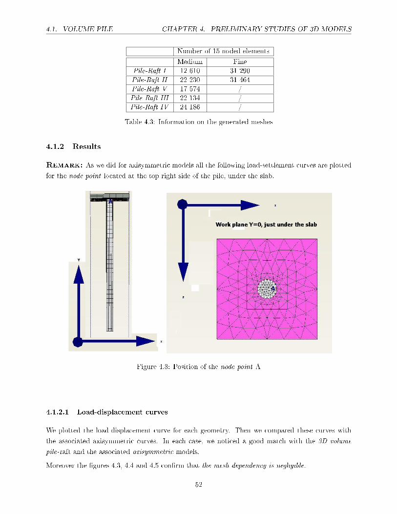
4.1.2 Results
Remark: As we did for axisymmetric models all the following load-settlement curves are plotted
for the node point located at the top right side of the pile, under the slab.
Figure 4.3: Position of the node point A
4.1.2.1 Load-displacement curves
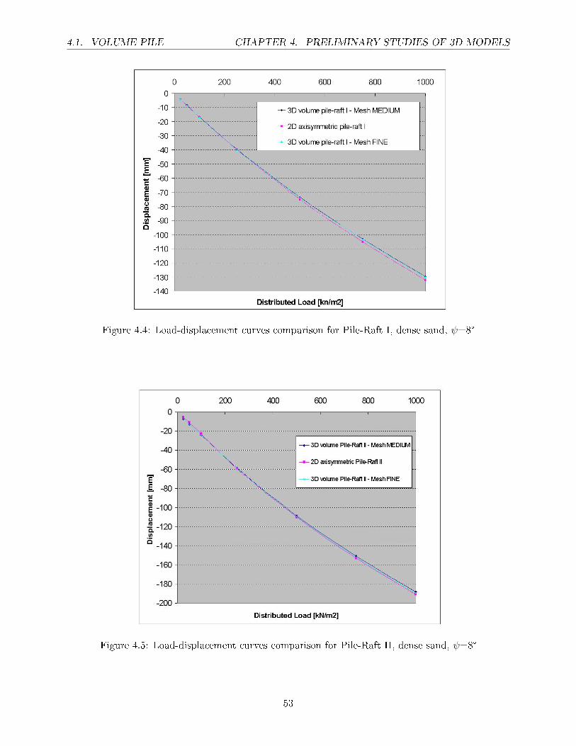
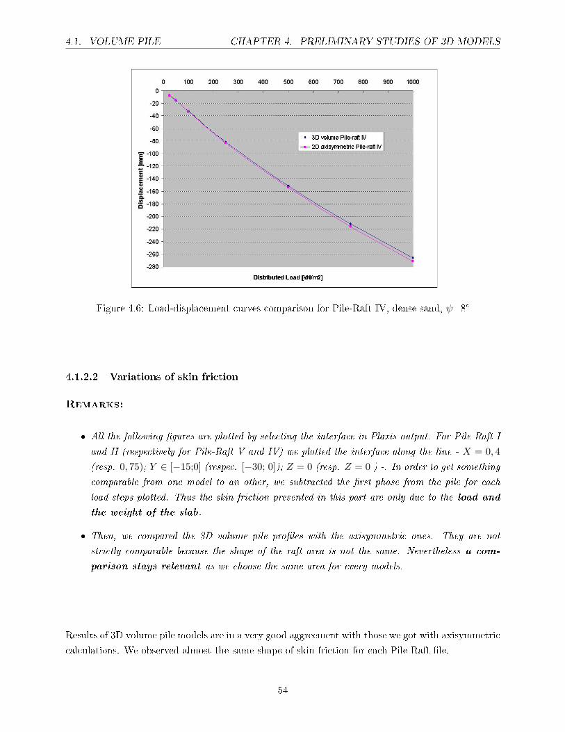
We plotted the load-displacement curve for each geometry. Then we compared these curves with
the associated axisymmetric curves. In each case, we noticed a good match with the 3D volume
pile-raft and the associated axisymmetric models.
Moreover the �gures 4.3, 4.4 and 4.5 con�rm that the mesh dependency is negligible.
52
4.1. VOLUME PILE CHAPTER 4. PRELIMINARY STUDIES OF 3D MODELS
Figure 4.4: Load-displacement curves comparison for Pile-Raft I, dense sand, ψ=8°
Figure 4.5: Load-displacement curves comparison for Pile-Raft II, dense sand, ψ=8°
53
4.1. VOLUME PILE CHAPTER 4. PRELIMINARY STUDIES OF 3D MODELS
Figure 4.6: Load-displacement curves comparison for Pile-Raft IV, dense sand, ψ=8°
4.1.2.2 Variations of skin friction
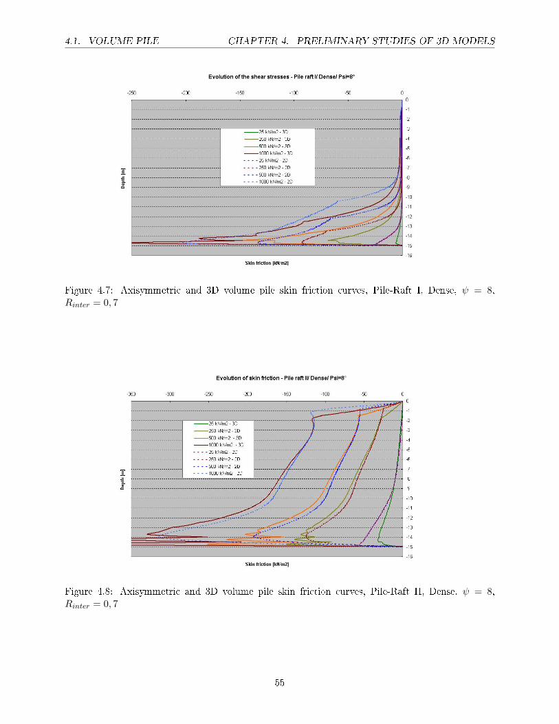
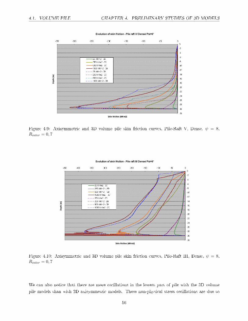
Remarks:
� All the following �gures are plotted by selecting the interface in Plaxis output. For Pile-Raft I
and II (respectively for Pile-Raft V and IV) we plotted the interface along the line - X = 0, 4(resp. 0, 75); Y ∈ [−15;0] (respec. [−30; 0]); Z = 0 (resp. Z = 0 ) -. In order to get something
comparable from one model to an other, we subtracted the �rst phase from the pile for each
load steps plotted. Thus the skin friction presented in this part are only due to the load and
the weight of the slab.
� Then, we compared the 3D volume pile pro�les with the axisymmetric ones. They are not
strictly comparable because the shape of the raft area is not the same. Nevertheless a com-
parison stays relevant as we choose the same area for every models.
Results of 3D volume pile models are in a very good aggreement with those we got with axisymmetric
calculations. We observed almost the same shape of skin friction for each Pile-Raft �le.
54
4.1. VOLUME PILE CHAPTER 4. PRELIMINARY STUDIES OF 3D MODELS
Figure 4.7: Axisymmetric and 3D volume pile skin friction curves, Pile-Raft I, Dense, ψ = 8,Rinter = 0, 7
Figure 4.8: Axisymmetric and 3D volume pile skin friction curves, Pile-Raft II, Dense, ψ = 8,Rinter = 0, 7
55
4.1. VOLUME PILE CHAPTER 4. PRELIMINARY STUDIES OF 3D MODELS
Figure 4.9: Axisymmetric and 3D volume pile skin friction curves, Pile-Raft V, Dense, ψ = 8,Rinter = 0, 7
Figure 4.10: Axisymmetric and 3D volume pile skin friction curves, Pile-Raft III, Dense, ψ = 8,Rinter = 0, 7
We can also notice that there are more oscillations in the lowest part of pile with the 3D volume
pile models than with 2D axisymmetric models. These non-physical stress oscillations are due to
56
4.1. VOLUME PILE CHAPTER 4. PRELIMINARY STUDIES OF 3D MODELS
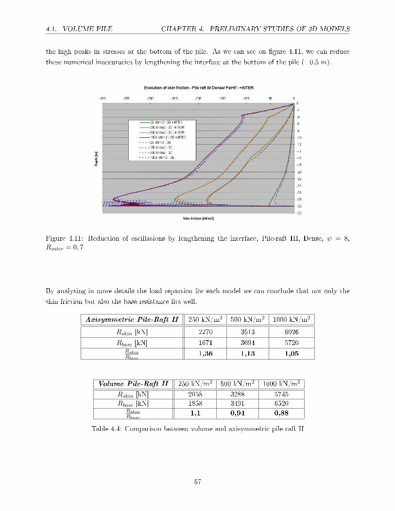
the high peaks in stresses at the bottom of the pile. As we can see on �gure 4.11, we can reduce
these numerical inaccuracies by lengthening the interface at the bottom of the pile (+0,5 m).
Figure 4.11: Reduction of oscillations by lengthening the interface, Pile-raft III, Dense, ψ = 8,Rinter = 0, 7
By analysing in more details the load repartion for each model we can conclude that not only the
skin friction but also the base resistance �ts well.
Axisymmetric Pile-Raft II 250 kN/m2 500 kN/m2 1000 kN/m2
Rskin [kN] 2270 3513 6026
Rbase [kN] 1671 3094 5720Rskin
Rbase1,36 1,13 1,05
Volume Pile-Raft II 250 kN/m2 500 kN/m2 1000 kN/m2
Rskin [kN] 2058 3288 5745
Rbase [kN] 1858 3491 6520Rskin
Rbase1,1 0,94 0,88
Table 4.4: Comparison between volume and axisymmetric pile raft II
57
4.1. VOLUME PILE CHAPTER 4. PRELIMINARY STUDIES OF 3D MODELS
Remarks: The following values have been calculated without subtracting the weight of the pile
and of the raft. For the volume pile, we estimated Rbase and Rskin by reading in Plaxis output the
normal force values N at the top and at the bottom of the pile. Then we considered that: Rbase=
Nbottom and Rskin= Ntop-Nbottom.
4.1.2.3 Some remarks about parameters
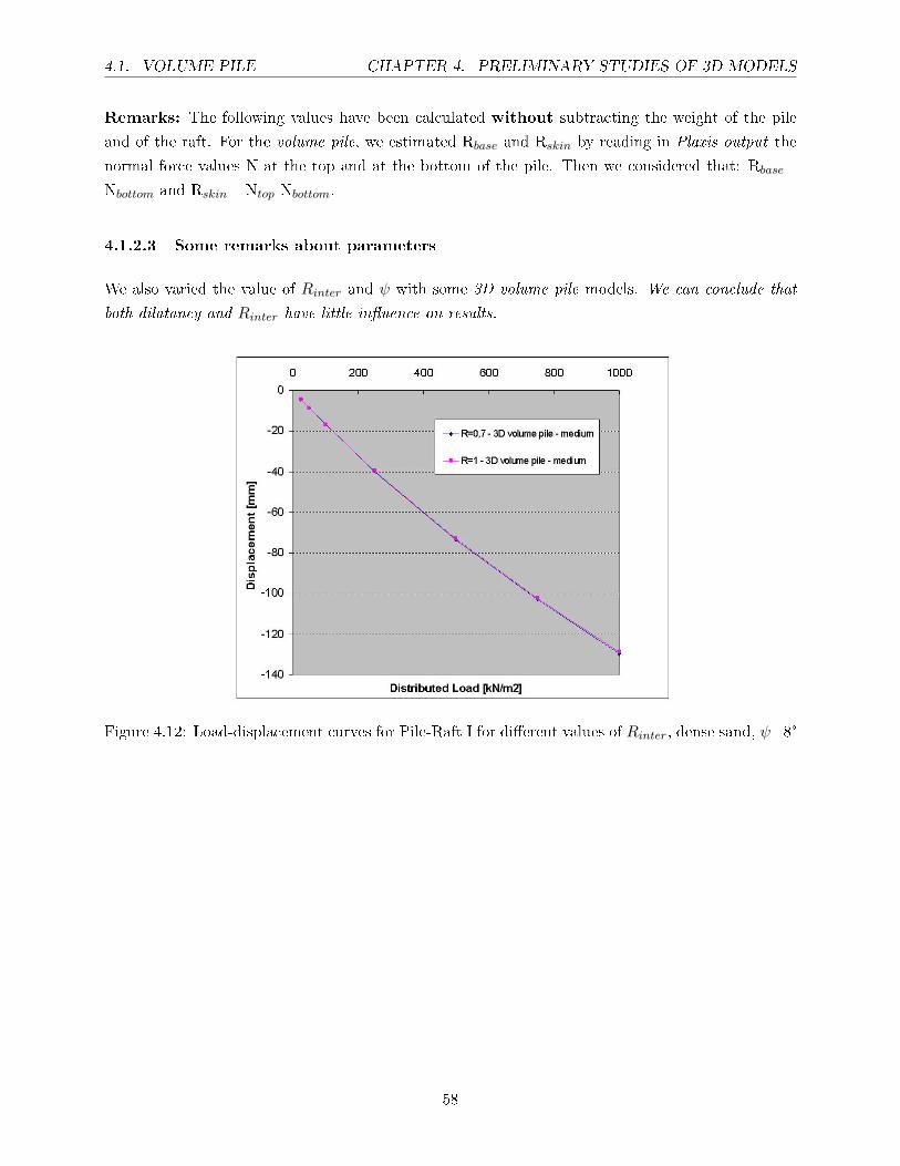
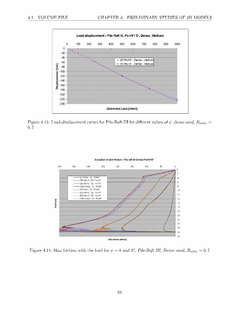
We also varied the value of Rinter and ψ with some 3D volume pile models. We can conclude that
both dilatancy and Rinter have little in�uence on results.
Figure 4.12: Load-displacement curves for Pile-Raft I for di�erent values of Rinter, dense sand, ψ=8°
58
4.1. VOLUME PILE CHAPTER 4. PRELIMINARY STUDIES OF 3D MODELS
Figure 4.13: Load-displacement curves for Pile-Raft III for di�erent values of ψ, dense sand, Rinter =0, 7
Figure 4.14: Skin friction with the load for ψ = 8 and 0°, Pile-Raft III, Dense sand, Rinter = 0, 7
59
4.2. EMBEDDED PILE CHAPTER 4. PRELIMINARY STUDIES OF 3D MODELS
4.2 Embedded pile
An embedded pile is a pile composed of beam elements that can be placed in arbitrary direction
in the sub-soil (irrespective from the alignment of soil volume elements) and that interacts with
the sub-soil by means of special interface elements. The interaction may involve a skin resistance
as well as a foot resistance. Although an embedded pile does not occupy volume, a particular
volume around the pile (elastic zone) is assumed in which plastic soil behaviour is excluded. The
size of this zone is based on the (equivalent) pile diameter according to the corresponding embedded
pile material data set. This makes the pile almost behave like a volume pile. Nevertheless, when
creating embedded piles no corresponding geometry points are created. Thus, contrary to volume
pile, embedded piles do not in�uence the �nite element mesh as generated from the geometry model.
So the mesh re�nement is lower and we save calculation time. 1
In contrast to what is common in the Finite Element Method, the bearing capacity of an embedded
pile is considered to be an input parameter rather than the result of the �nite element calculation.
Plaxis gives us the possibility to enter the skin resistance pro�le in three ways:
� Linear: The user enters the skin resistance at the pile top and the skin resistance at the pile
bottom. The skin resistance is de�ned as linear along the pile. This way of de�ning the pile
skin resistance is mostly applicable to piles in a homogeneous soil layer.
� Multi-linear: The skin resistance is de�ned in a table at di�erent positions along the pile.
Multi-linear can be used to take into account inhomogeneous or multiple soil layers with
di�erent properties and, as a result, di�erent resistances.
� Layer dependent, can be used to relate the local skin resistance to the strength properties of
the soil layer in which the pile is located, and the interface strength reduction factor Rinter,
as de�ned in the material data set on the corresponding soil layer. Using this approach the
pile bearing capacity is based on the stress state in the soil, and thus unknown at the start of
a calculation. Nevertheless an overall maximum resistance can be speci�ed before to avoid an
undesired too high value at the end.
We performed another set of calculations by modeling the previous geometries using embedded
piles. This study gave us the possibility to test the reliability of this new feature to model pile-raft
structures.
4.2.1 Embedded pile-raft
For this study, we focused our calculations on the two �rst geometries named Pile-Raft I and Pile-
Raft II. We took exactly the same geometries by using embedded piles instead of volume piles. We
1See Plaxis manual for more details about embedded piles
60
4.2. EMBEDDED PILE CHAPTER 4. PRELIMINARY STUDIES OF 3D MODELS
considered the pile to raft connection as rigid. As mentioned previously the capacity of the pile is an
input parameter for an embedded pile so we had to de�ne the most relevant skin friction distribution
and base resistance. This is the reason why we tested each possibility o�ered by Plaxis to try to
con�gure in a proper way this new tool.
4.2.1.1 Finite element models
The parameters we examined for the embedded pile are the same as those desribed previously for
the volume pile. We performed calculations for only one material, the dense sand with Rinter = 0, 7.The load is modeled as a distributed load on the slab. Two di�erent meshes with di�erent levels of
re�nement had been used. The following tables sum up the most important parameters.
Name Thicknessslab Depthmodel Lengthpile Diameterpile WidthraftWidthraft
Diameterpile
Pile-Raft I 0,5 m 40 m 15 m 0,8 m 1,8 m 2,25
Pile-Raft II 0,5 m 40 m 15 m 0,8 m 4,4 m 5,5
Table 4.5: Basic parameters of each geometry
Parameter Symbol Dense sand Concrete (slab) Unit
Material model Model Hardening Soil Linear Elastic -
Unsaturated weigth γunsat 19 25 kN/m3
Saturated weigth γsat 21 25 kN/m3
Permeability k 1 0 m/day
Eref50 60 000 kN/m3
Sti�ness Erefoed 60 000 3E7 kN/m3
Erefur 1,8E5 kN/m3
Power m 0,55
Poisson ratio νur 0,2 0,2 -
Dilatancy y 8 °
Friction angle f 38 °
Cohesion cref 0,1 kN/m2
Lateral pressure coe�. K0 1-sinf -
Failure ratio Rf 0,9 -
Table 4.6: Soil parameters
61
4.2. EMBEDDED PILE CHAPTER 4. PRELIMINARY STUDIES OF 3D MODELS
Parameter Name Value Unit
Young´s modulus E 3.107 kN/m3
Weight γ 5 kN/m3
Properties type Type Massive circular pile -
Diameter dpile 0,8 m
Length Lpile 15 m
Table 4.7: Material properties of the embedded pile
Number of 15-noded elements
Medium Fine
Pile-Raft I 16 048 36 120
Pile-Raft II 14 300 36 800
Table 4.8: Information on generated meshes
Figure 4.15: Details about an embedded pile-raft geometry in 3D, �ne mesh, pile-raft II
62
4.2. EMBEDDED PILE CHAPTER 4. PRELIMINARY STUDIES OF 3D MODELS
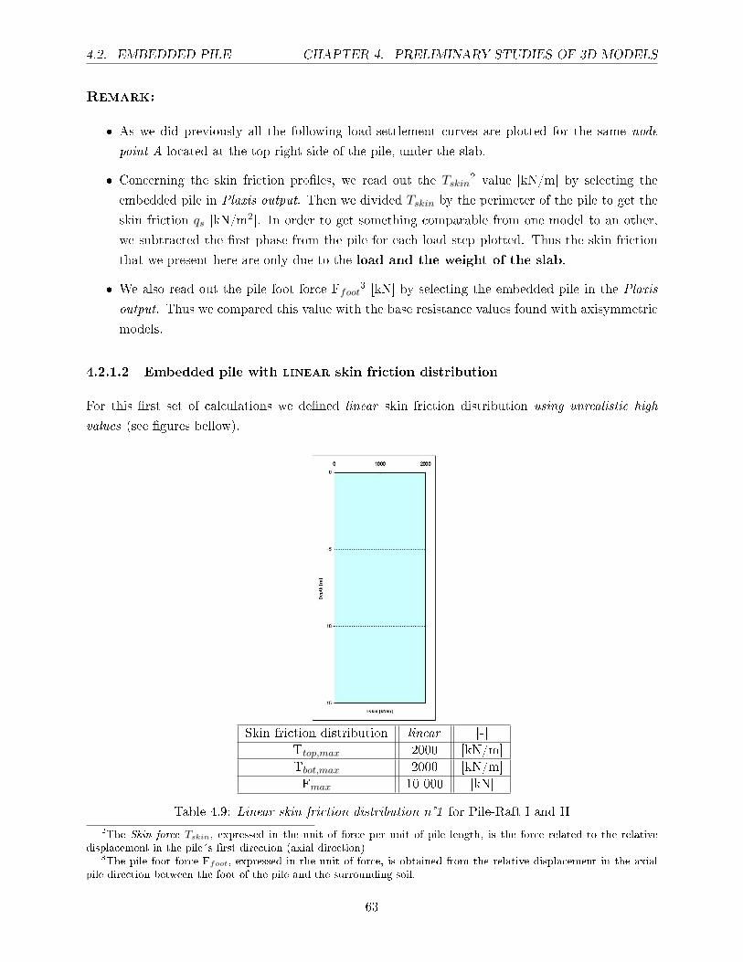
Remark:
� As we did previously all the following load-settlement curves are plotted for the same node
point A located at the top right side of the pile, under the slab.
� Concerning the skin friction pro�les, we read out the Tskin2 value [kN/m] by selecting the
embedded pile in Plaxis output. Then we divided Tskin by the perimeter of the pile to get the
skin friction qs [kN/m2]. In order to get something comparable from one model to an other,
we subtracted the �rst phase from the pile for each load step plotted. Thus the skin friction
that we present here are only due to the load and the weight of the slab.
� We also read out the pile foot force Ffoot3 [kN] by selecting the embedded pile in the Plaxis
output. Thus we compared this value with the base resistance values found with axisymmetric
models.
4.2.1.2 Embedded pile with linear skin friction distribution
For this �rst set of calculations we de�ned linear skin friction distribution using unrealistic high
values (see �gures bellow).
Skin friction distribution linear [-]
Ttop,max 2000 [kN/m]
Tbot,max 2000 [kN/m]
Fmax 10 000 [kN]
Table 4.9: Linear skin friction distribution n°1 for Pile-Raft I and II
2The Skin force Tskin, expressed in the unit of force per unit of pile length, is the force related to the relativedisplacement in the pile´s �rst direction (axial direction)
3The pile foot force Ffoot, expressed in the unit of force, is obtained from the relative displacement in the axialpile direction between the foot of the pile and the surrounding soil.
63
4.2. EMBEDDED PILE CHAPTER 4. PRELIMINARY STUDIES OF 3D MODELS
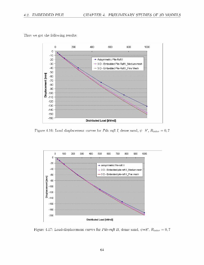
Thus we got the following results:
Figure 4.16: Load-displacement curves for Pile-raft I, dense sand, ψ=8°, Rinter = 0, 7
Figure 4.17: Load-displacement curves for Pile-raft II, dense sand, ψ=8°, Rinter = 0, 7
64
4.2. EMBEDDED PILE CHAPTER 4. PRELIMINARY STUDIES OF 3D MODELS
Load=1000 kN/m2 Settlement [cm]
axisymmetric Pile-Raft I -13,2
Embedded Pile-Raft I_Medium -14,8
Embedded Pile-Raft I_Fine -15,8
axisymmetric Pile-Raft II -19,1
Embedded Pile-Raft II_Medium -19,6
Embedded Pile-Raft II_Fine -19,9
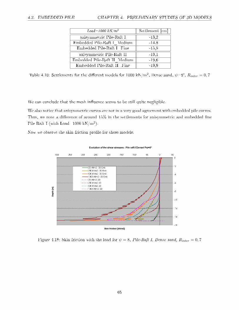
Table 4.10: Settlements for the di�erent models for 1000 kN/m2, Dense sand, ψ=8°, Rinter = 0, 7
We can conclude that the mesh in�uence seems to be still quite negligible.
We also notice that axisymmetric curves are not in a very good agreement with embedded pile curves.
Thus, we note a di�erence of around 15% in the settlements for axisymmetric and embedded �ne
Pile-Raft I (with Load=1000 kN/m2).
Now we observe the skin friction pro�le for these models:
Figure 4.18: Skin friction with the load for ψ = 8, Pile-Raft I, Dense sand, Rinter = 0, 7
65
4.2. EMBEDDED PILE CHAPTER 4. PRELIMINARY STUDIES OF 3D MODELS
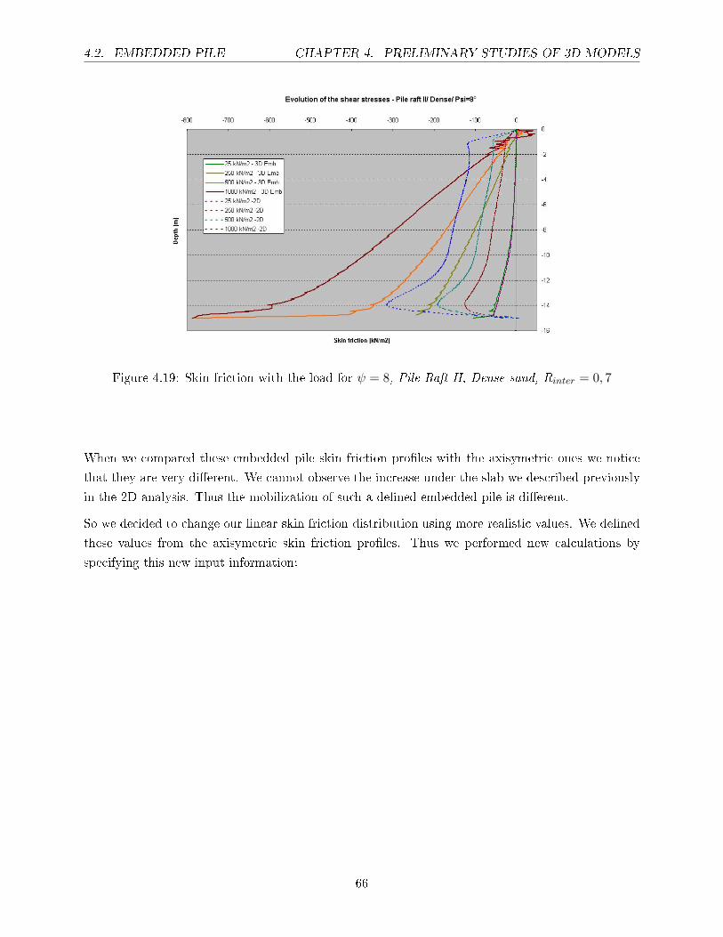
Figure 4.19: Skin friction with the load for ψ = 8, Pile-Raft II, Dense sand, Rinter = 0, 7
When we compared these embedded pile skin friction pro�les with the axisymetric ones we notice
that they are very di�erent. We cannot observe the increase under the slab we described previously
in the 2D analysis. Thus the mobilization of such a de�ned embedded pile is di�erent.
So we decided to change our linear skin friction distribution using more realistic values. We de�ned
these values from the axisymetric skin friction pro�les. Thus we performed new calculations by
specifying this new input information:
66
4.2. EMBEDDED PILE CHAPTER 4. PRELIMINARY STUDIES OF 3D MODELS
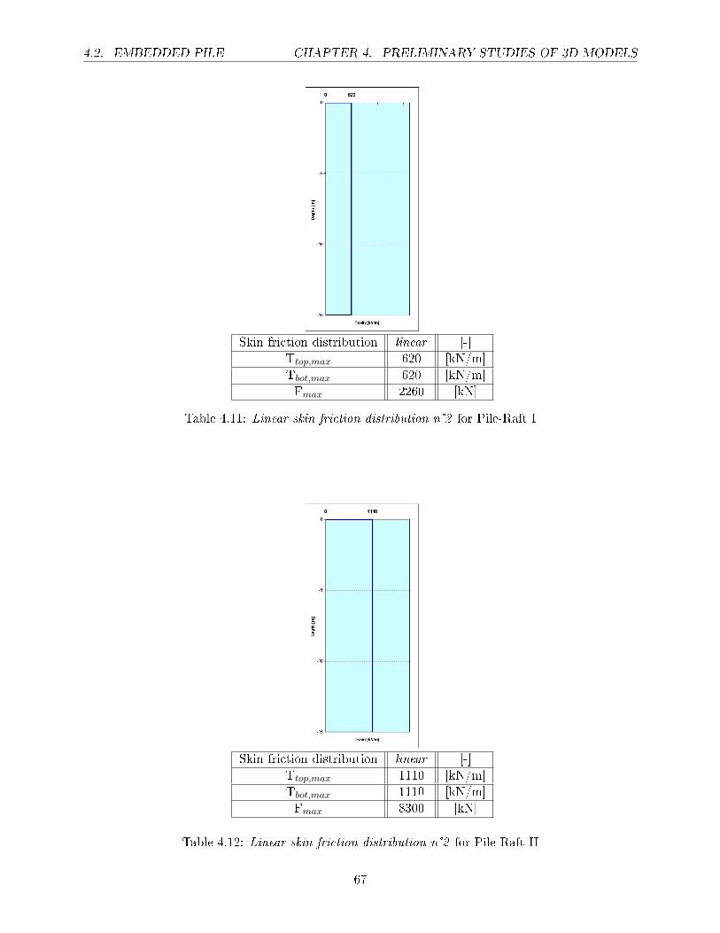
Skin friction distribution linear [-]
Ttop,max 620 [kN/m]
Tbot,max 620 [kN/m]
Fmax 2260 [kN]
Table 4.11: Linear skin friction distribution n°2 for Pile-Raft I
Skin friction distribution linear [-]
Ttop,max 1110 [kN/m]
Tbot,max 1110 [kN/m]
Fmax 8300 [kN]
Table 4.12: Linear skin friction distribution n°2 for Pile-Raft II
67
4.2. EMBEDDED PILE CHAPTER 4. PRELIMINARY STUDIES OF 3D MODELS
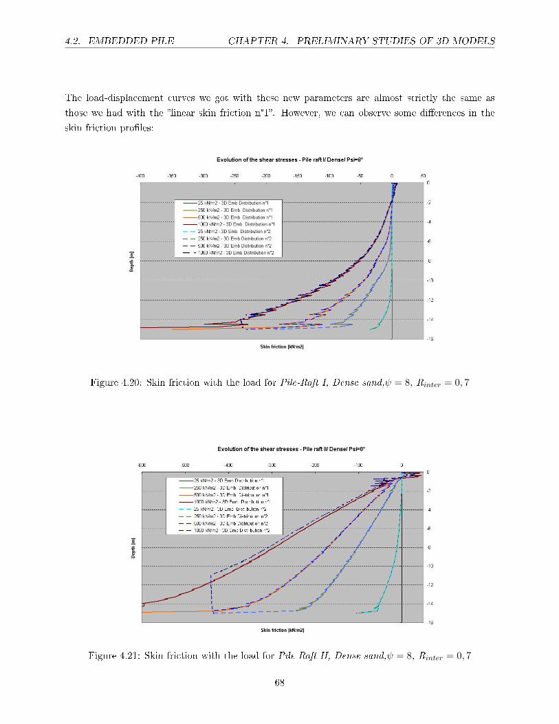
The load-displacement curves we got with these new parameters are almost strictly the same as
those we had with the �linear skin friction n°1�. However, we can observe some di�erences in the
skin friction pro�les:
Figure 4.20: Skin friction with the load for Pile-Raft I, Dense sand,ψ = 8, Rinter = 0, 7
Figure 4.21: Skin friction with the load for Pile-Raft II, Dense sand,ψ = 8, Rinter = 0, 7
68
4.2. EMBEDDED PILE CHAPTER 4. PRELIMINARY STUDIES OF 3D MODELS
For the lowest load, the pro�les are exactly the same for the distribution -n°1 or n°2- . Nevertheless,
with the highest load and the input � linear skin friction distribution n°2 �, the skin friction reaches
the input value and stops growing.
To conclude we can say that neither � linear skin friction distribution n°2 � nor � linear skin friction
distribution n°1� leads to a skin friction pro�le in aggrement with the realistic one.
4.2.1.3 Embedded pile with multilinear skin friction distribution
For this second set of calculations we tested three di�erent multilinear skin friction distributions.
Input:
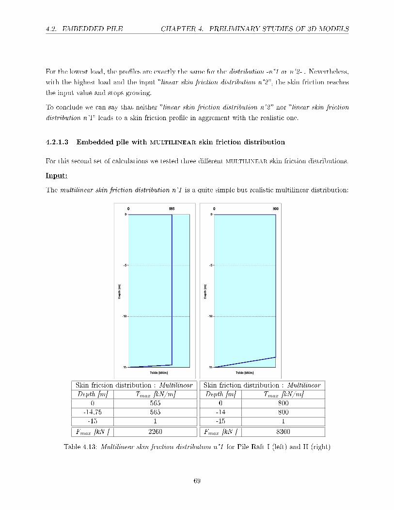
The multilinear skin friction distribution n°1 is a quite simple but realistic multilinear distribution:
Skin friction distribution : Multilinear
Depth [m] Tmax [kN/m]
0 565
-14,75 565
-15 1
Fmax [kN ] 2260
Skin friction distribution : Multilinear
Depth [m] Tmax [kN/m]
0 800
-14 800
-15 1
Fmax [kN ] 8300
Table 4.13: Multilinear skin friction distribution n°1 for Pile-Raft I (left) and II (right)
69
4.2. EMBEDDED PILE CHAPTER 4. PRELIMINARY STUDIES OF 3D MODELS
The multilinear skin friction distribution n°2 is the same as multilinear skin friction distribution
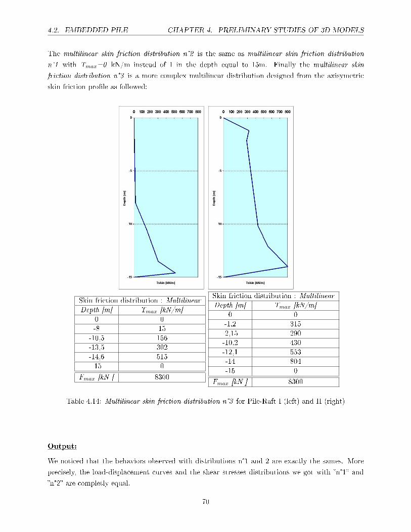
n°1 with Tmax=0 kN/m instead of 1 in the depth equal to 15m. Finally the multilinear skin
friction distribution n°3 is a more complex multilinear distribution designed from the axisymetric
skin friction pro�le as followed:
Skin friction distribution : Multilinear
Depth [m] Tmax [kN/m]
0 0
-8 15
-10,5 156
-13,5 302
-14,6 515
-15 0
Fmax [kN ] 8300
Skin friction distribution : Multilinear
Depth [m] Tmax [kN/m]
0 0
-1,2 315
-2,15 290
-10,2 430
-12,1 553
-14 804
-15 0
Fmax [kN ] 8300
Table 4.14: Multilinear skin friction distribution n°3 for Pile-Raft I (left) and II (right)
Output:
We noticed that the behaviors observed with distributions n°1 and 2 are exactly the sames. More
precisely, the load-displacement curves and the shear stresses distributions we got with �n°1� and
�n°2� are completly equal.
70
4.2. EMBEDDED PILE CHAPTER 4. PRELIMINARY STUDIES OF 3D MODELS
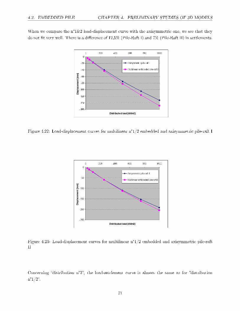
When we compare the n°1&2 load-displacement curve with the axisymmetric one, we see that they
do not �t very well. There is a di�erence of 12,5% (Pile-Raft I) and 7% (Pile-Raft II) in settlements.
Figure 4.22: Load-displacement curves for multilinear n°1/2 embedded and axisymmetric pile-raft I
Figure 4.23: Load-displacement curves for multilinear n°1/2 embedded and axisymmetric pile-raftII
Concerning �distribution n°3�, the load-settlement curve is almost the same as for �distribution
n°1/2�.
71
4.2. EMBEDDED PILE CHAPTER 4. PRELIMINARY STUDIES OF 3D MODELS
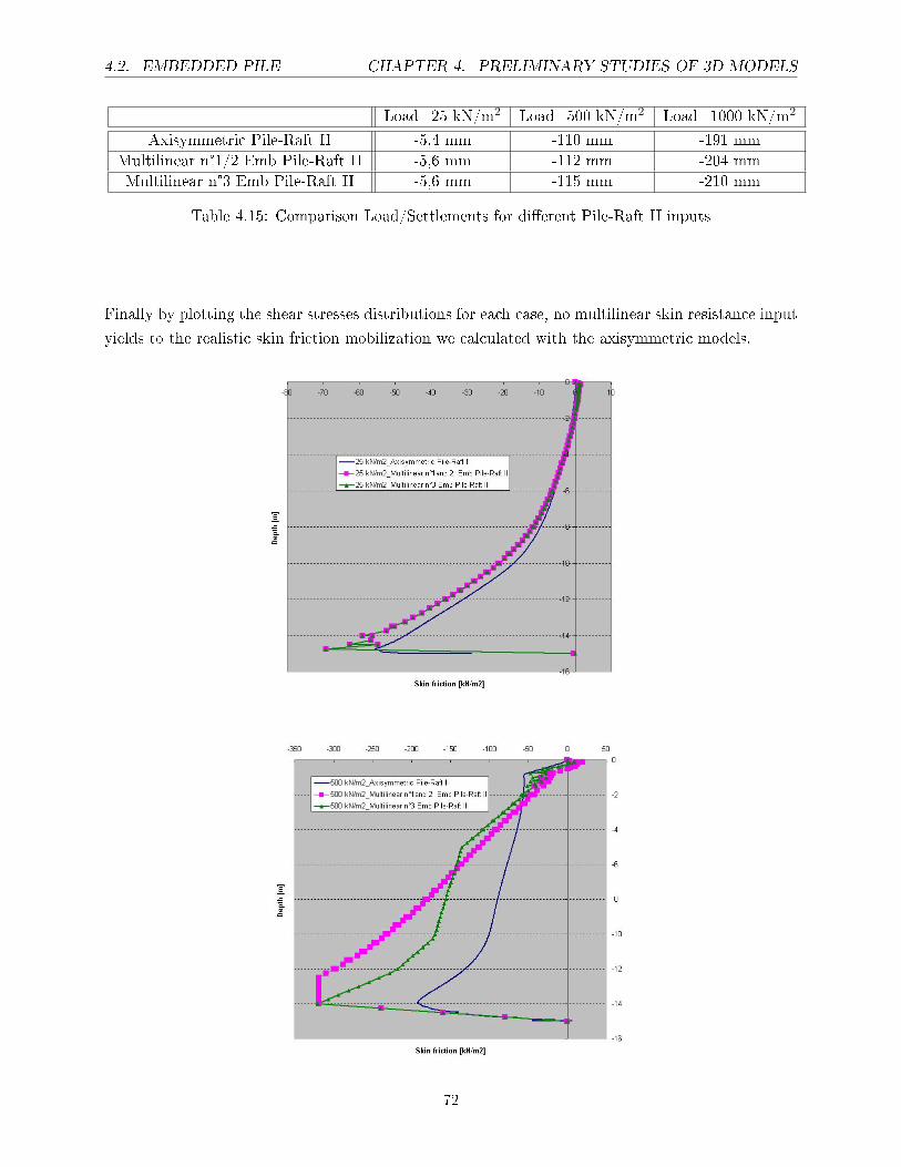
Load=25 kN/m2 Load=500 kN/m2 Load=1000 kN/m2
Axisymmetric Pile-Raft II -5,4 mm -110 mm -191 mm
Multilinear n°1/2 Emb Pile-Raft II -5,6 mm -112 mm -204 mm
Multilinear n°3 Emb Pile-Raft II -5,6 mm -115 mm -210 mm
Table 4.15: Comparison Load/Settlements for di�erent Pile-Raft II inputs
Finally by plotting the shear stresses distributions for each case, no multilinear skin resistance input
yields to the realistic skin friction mobilization we calculated with the axisymmetric models.
72
4.2. EMBEDDED PILE CHAPTER 4. PRELIMINARY STUDIES OF 3D MODELS
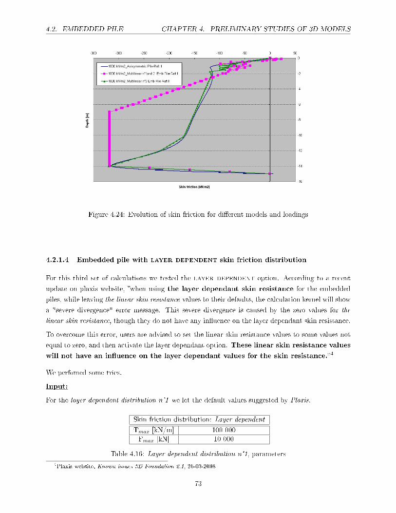
Figure 4.24: Evolution of skin friction for di�erent models and loadings
4.2.1.4 Embedded pile with layer dependent skin friction distribution
For this third set of calculations we tested the layer dependent option. According to a recent
update on plaxis website, �when using the layer dependant skin resistance for the embedded
piles, while leaving the linear skin resistance values to their defaults, the calculation kernel will show
a "severe divergence" error message. This severe divergence is caused by the zero values for the
linear skin resistance, though they do not have any in�uence on the layer dependant skin resistance.
To overcome this error, users are advised to set the linear skin resistance values to some values not
equal to zero, and then activate the layer dependant option. These linear skin resistance values
will not have an in�uence on the layer dependant values for the skin resistance.�4
We perfomed some tries.
Input:
For the layer dependent distribution n°1 we let the default values suggested by Plaxis.
Skin friction distribution: Layer dependent
Tmax [kN/m] 100 000
Fmax [kN] 10 000
Table 4.16: Layer dependent distribution n°1, parameters
4Plaxis website, Known issues 3D Foundation 2.1, 26-03-2008
73
4.2. EMBEDDED PILE CHAPTER 4. PRELIMINARY STUDIES OF 3D MODELS
As we explained in the introduction of this section, we did not let the default values for the linear
skin resistance. We input 1.
For the layer dependent distribution n°1bis we used the values as described in the previous table,
but we input 2000 for the linear skin resistance.
We tested with dense sand, Rinter = 0, 7.
Output:
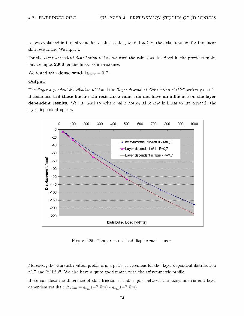
The �layer dependent distribution n°1� and the �layer dependent distribution n°1bis� perfectly match.
It con�rmed that these linear skin resistance values do not have an in�uence on the layer
dependent results. We just need to write a value not equal to zero in linear to use correctly the
layer dependant option.
Figure 4.25: Comparison of load-displacement curves
Moreover, the skin distribution pro�le is in a perfect agreement for the �layer dependent distribution
n°1� and �n°1Bis�. We also have a quite good match with the axisymmetric pro�le.
If we calculate the di�erence of skin friction at half a pile between the axisymmetric and layer
dependent results : ∆7,5m = qs2D(−7, 5m) - qs3D(−7, 5m)
74
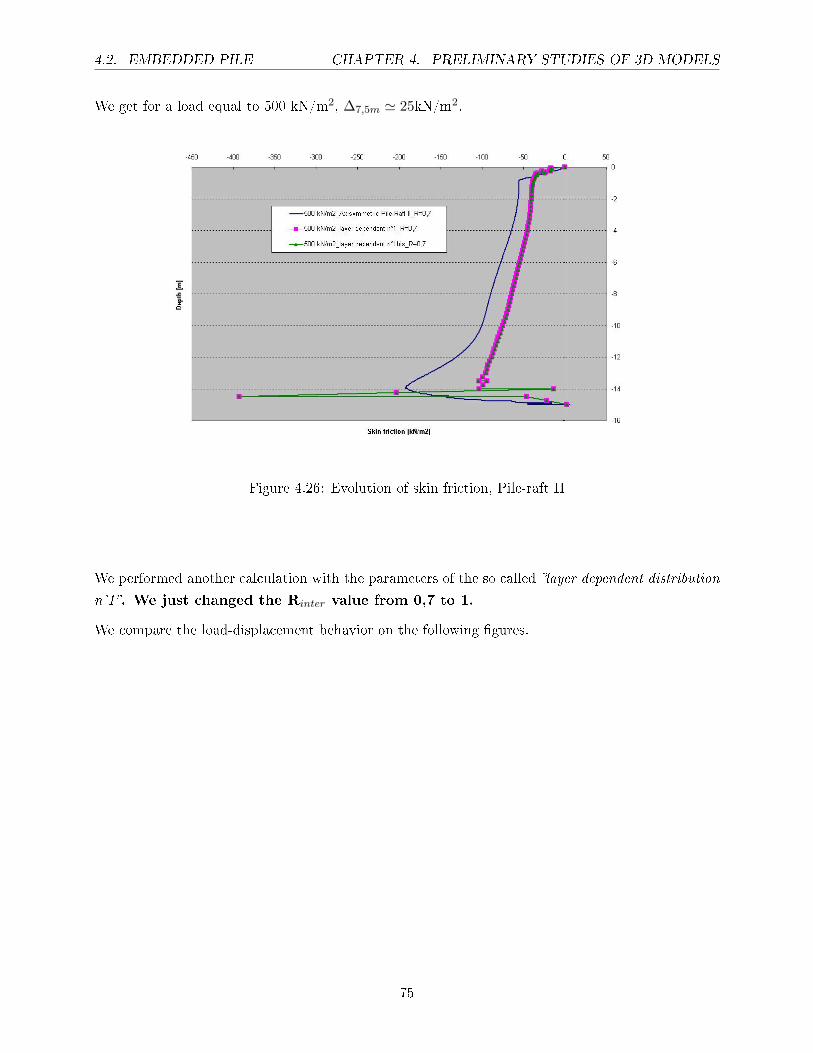
4.2. EMBEDDED PILE CHAPTER 4. PRELIMINARY STUDIES OF 3D MODELS
We get for a load equal to 500 kN/m2, ∆7,5m ' 25kN/m2.
Figure 4.26: Evolution of skin friction, Pile-raft II
We performed another calculation with the parameters of the so called �layer dependent distribution
n°1�. We just changed the Rinter value from 0,7 to 1.
We compare the load-displacement behavior on the following �gures.
75
4.2. EMBEDDED PILE CHAPTER 4. PRELIMINARY STUDIES OF 3D MODELS
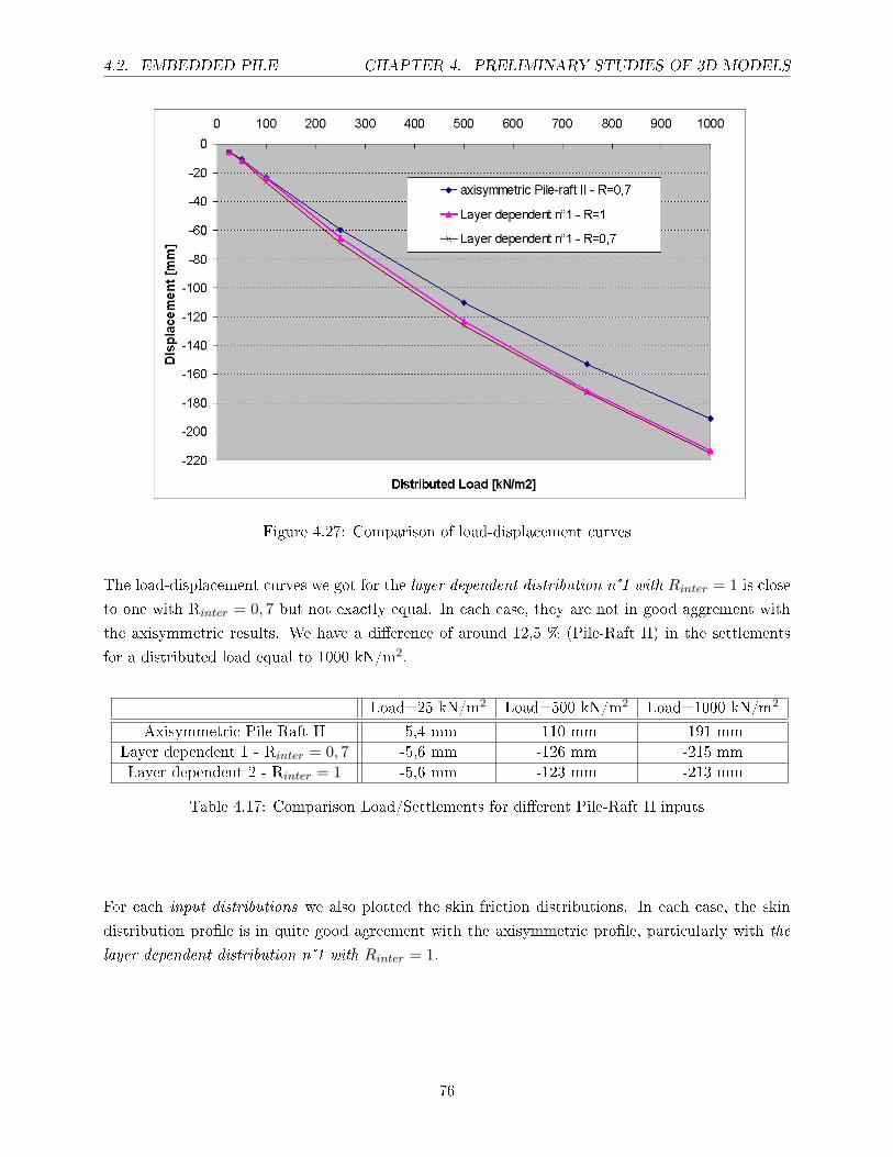
Figure 4.27: Comparison of load-displacement curves
The load-displacement curves we got for the layer dependent distribution n°1 with Rinter = 1 is close
to one with Rinter = 0, 7 but not exactly equal. In each case, they are not in good aggrement with
the axisymmetric results. We have a di�erence of around 12,5 % (Pile-Raft II) in the settlements
for a distributed load equal to 1000 kN/m2.
Load=25 kN/m2 Load=500 kN/m2 Load=1000 kN/m2
Axisymmetric Pile-Raft II -5,4 mm -110 mm -191 mm
Layer dependent 1 - Rinter = 0, 7 -5,6 mm -126 mm -215 mm
Layer dependent 2 - Rinter = 1 -5,6 mm -123 mm -213 mm
Table 4.17: Comparison Load/Settlements for di�erent Pile-Raft II inputs
For each input distributions we also plotted the skin friction distributions. In each case, the skin
distribution pro�le is in quite good agreement with the axisymmetric pro�le, particularly with the
layer dependent distribution n°1 with Rinter = 1.
76
4.2. EMBEDDED PILE CHAPTER 4. PRELIMINARY STUDIES OF 3D MODELS
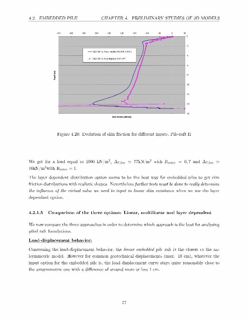
Figure 4.28: Evolution of skin friction for di�erent inputs, Pile-raft II
We get for a load equal to 1000 kN/m2, ∆7,5m ' 77kN/m2 with Rinter = 0, 7 and ∆7,5m '16kN/m2with Rinter = 1.
The layer dependent distribution option seems to be the best way for embedded piles to get skin
friction distributions with realistic shapes. Nevertheless further tests must be done to really determine
the in�uence of the virtual value we need to input in linear skin resistance when we use the layer
dependant option.
4.2.1.5 Comparison of the three options: Linear, multilinear and layer dependent
We now compare the three approaches in order to determine which approach is the best for analysing
piled raft foundations.
Load-displacement behavior:
Concerning the load-displacement behavior, the linear embedded pile raft is the closest to the ax-
isymmetric model. However for common geotechnical displacements (max. 10 cm), whatever the
input option for the embedded pile is, the load displacement curve stays quite reasonably close to
the axisymmetric one with a di�erence of around more or less 1 cm.
77
4.2. EMBEDDED PILE CHAPTER 4. PRELIMINARY STUDIES OF 3D MODELS
Load=25 kN/m2 Load=500 kN/m2 Load=1000 kN/m2
Axisymmetric -5,4 mm -110 mm -191 mm
Linear embedded +3,7 % +0,9% +3,7%
Multilinear embedded +3,7 % +4,5% +12%
Layer dependent embedded +3,7 % +14,5% +12,6%
Table 4.18: Displacement with the load, for Pile-Raft II
Figure 4.29: Load-displacement curves for Pile-Raft II
Pile-raft behavior:
According to the skin friction distributions presented previously, we saw that the mobilization of the
embedded pile-raft foundation and the axisymetric pile-raft foundation is di�erent. So we analysed
in more details the load repartion for each model. The following values have been calculated by
subtracting the weight of the pile and of the raft .
78
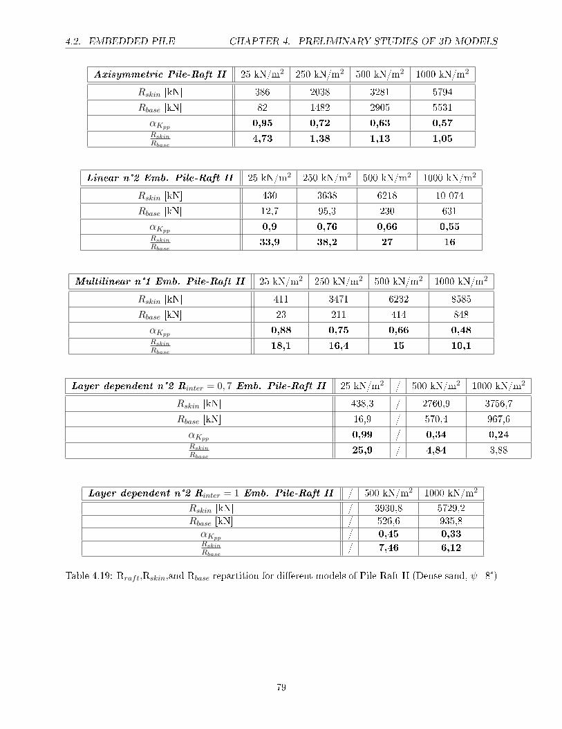
4.2. EMBEDDED PILE CHAPTER 4. PRELIMINARY STUDIES OF 3D MODELS
Axisymmetric Pile-Raft II 25 kN/m2 250 kN/m2 500 kN/m2 1000 kN/m2
Rskin [kN] 386 2038 3281 5794
Rbase [kN] 82 1482 2905 5531
αKpp 0,95 0,72 0,63 0,57Rskin
Rbase4,73 1,38 1,13 1,05
Linear n°2 Emb. Pile-Raft II 25 kN/m2 250 kN/m2 500 kN/m2 1000 kN/m2
Rskin [kN] 430 3638 6218 10 074
Rbase [kN] 12,7 95,3 230 631
αKpp 0,9 0,76 0,66 0,55Rskin
Rbase33,9 38,2 27 16
Multilinear n°1 Emb. Pile-Raft II 25 kN/m2 250 kN/m2 500 kN/m2 1000 kN/m2
Rskin [kN] 411 3471 6232 8585
Rbase [kN] 23 211 414 848
αKpp 0,88 0,75 0,66 0,48Rskin
Rbase18,1 16,4 15 10,1
Layer dependent n°2 Rinter = 0, 7 Emb. Pile-Raft II 25 kN/m2 / 500 kN/m2 1000 kN/m2
Rskin [kN] 438,3 / 2760,9 3756,7
Rbase [kN] 16,9 / 570,4 967,6
αKpp 0,99 / 0,34 0,24Rskin
Rbase25,9 / 4,84 3,88
Layer dependent n°2 Rinter = 1 Emb. Pile-Raft II / 500 kN/m2 1000 kN/m2
Rskin [kN] / 3930,8 5729,2
Rbase [kN] / 526,6 935,8
αKpp / 0,45 0,33Rskin
Rbase/ 7,46 6,12
Table 4.19: Rraft,Rskin,and Rbase repartition for di�erent models of Pile-Raft II (Dense sand, ψ=8°)
79
4.2. EMBEDDED PILE CHAPTER 4. PRELIMINARY STUDIES OF 3D MODELS
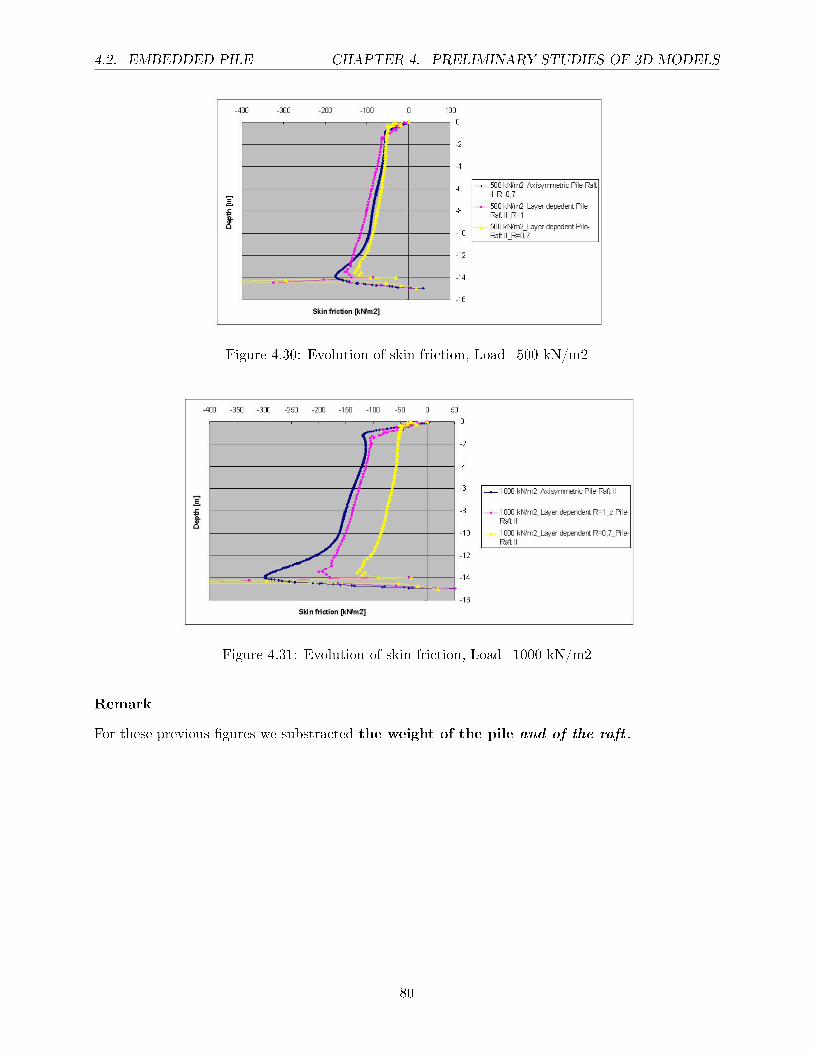
Figure 4.30: Evolution of skin friction, Load=500 kN/m2
Figure 4.31: Evolution of skin friction, Load=1000 kN/m2
Remark
For these previous �gures we substracted the weight of the pile and of the raft .
80
4.2. EMBEDDED PILE CHAPTER 4. PRELIMINARY STUDIES OF 3D MODELS
Axisymmetric Pile-Raft I 25 kN/m2 250 kN/m2 500 kN/m2 1000 kN/m2
Rskin [kN] 50,3 451,5 812,5 1426
Rbase [kN] 35,8 335,1 783 1768
αKpp 0,99 0,99 0,99 0,99Rskin
Rbase1,41 1,35 1,04 0,81
Linear n°2 Emb. Pile-Raft I 25 kN/m2 250 kN/m2 500 kN/m2 1000 kN/m2
Rskin [kN] 74 747 1463 2863
Rbase [kN] 4,6 35 85,1 203
αKpp 1 1 0,99 0,98Rskin
Rbase16 21,4 17,2 14,1
Multilinear n°1 Emb. Pile-Raft I 25 kN/m2 250 kN/m2 500 kN/m2 1000 kN/m2
Rskin [kN] 67 697 1400 2792
Rbase [kN] 9 65,2 123,5 252
αKpp 0,97 0,97 0,97 0,97Rskin
Rbase7,6 10,7 11,3 11,1
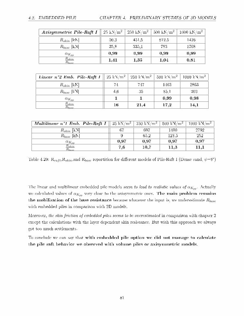
Table 4.20: Rraft,Rskin,and Rbase repartition for di�erent models of Pile-Raft I (Dense sand, ψ=8°)
The linear and multilinear embedded pile models seem to lead to realistic values of αKpp . Actually
we calculated values of αKpp very close to the axisymmetric ones. The main problem remains
the mobilization of the base resistance because whatever the input is, we underestimate Rbase
with embedded piles in comparison with 2D models.
Moreover, the skin friction of embedded piles seems to be overestimated in comparison with chapter 2
except the calculations with the layer dependent skin resistance. But with this approach we always
got too much settlements.
To conclude we can say that with embedded pile option we did not manage to calculate
the pile raft behavior we observed with volume piles or axisymmetric models.
81
Chapter 5
Group e�ect
- Analysis of the group e�ects in piled raft foundations -
The previous models gave us a �rst idea of a piled raft foundation behavior. These models took
into account the pile-soil interaction, the raft-soil interaction and the pile-raft interaction but not
the pile-pile interaction. Yet when the piles spacing is small, a partial geometry with a single pile
and one section of the raft is not accurate enough. We must consider the pile-pile interaction and
design more complex models with a group of piles.
In this chapter, we present some observations about the group e�ect in a piled raft foundation.
5.1 Presentation of calculations
We studied a piled raft foundations with 6×6 piles. Thus by using symetries we modeled only 9
piles. To study the in�uence of pile length and diameter as well as spacing between piles we designed
�ve di�erent geometries.
82
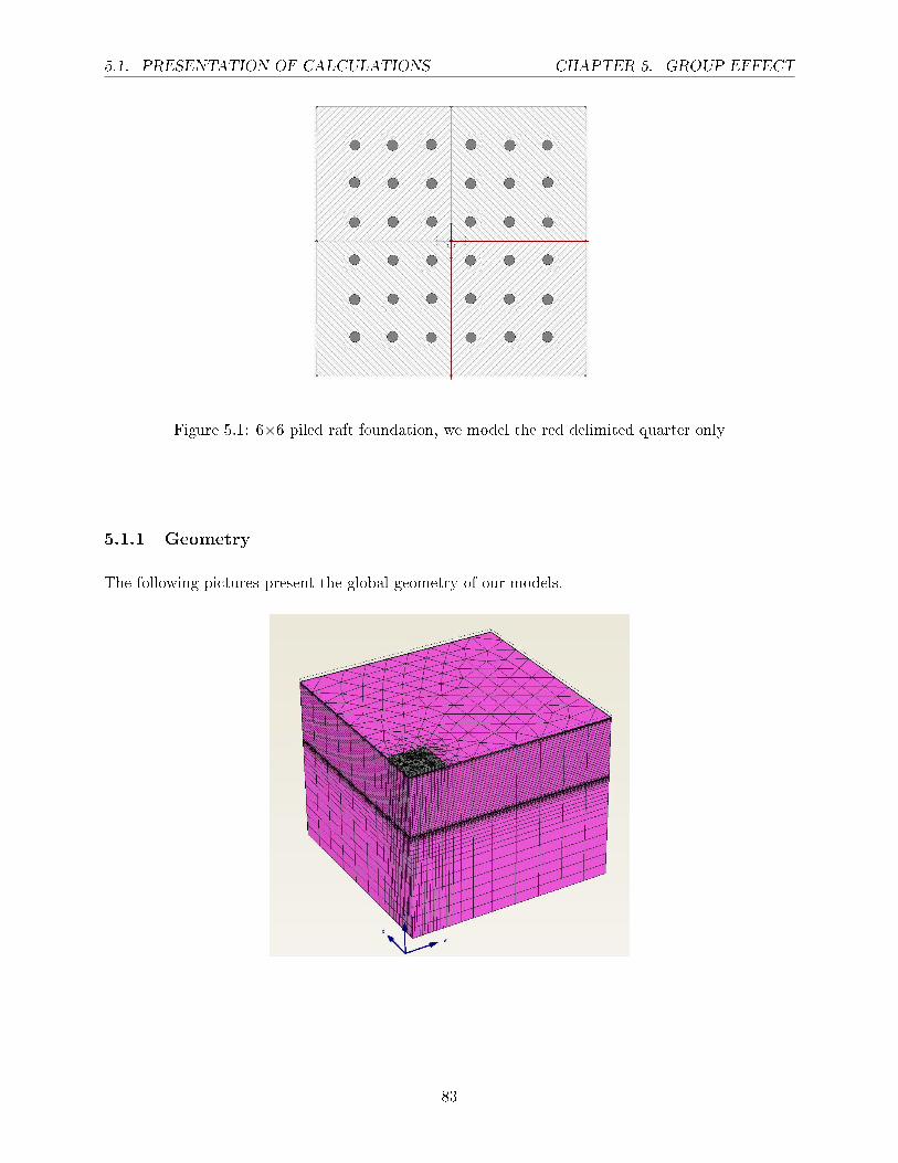
5.1. PRESENTATION OF CALCULATIONS CHAPTER 5. GROUP EFFECT
Figure 5.1: 6×6 piled raft foundation, we model the red delimited quarter only
5.1.1 Geometry
The following pictures present the global geometry of our models.
83
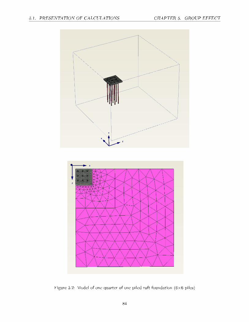
5.1. PRESENTATION OF CALCULATIONS CHAPTER 5. GROUP EFFECT
Figure 5.2: Model of one quarter of one piled raft foundation (6×6 piles)
84
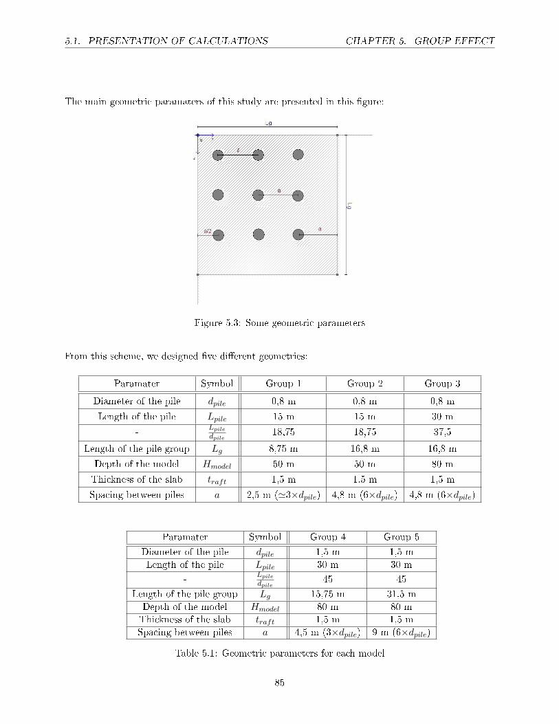
5.1. PRESENTATION OF CALCULATIONS CHAPTER 5. GROUP EFFECT
The main geometric paramaters of this study are presented in this �gure:
Figure 5.3: Some geometric parameters
From this scheme, we designed �ve di�erent geometries:
Paramater Symbol Group 1 Group 2 Group 3
Diameter of the pile dpile 0,8 m 0,8 m 0,8 m
Length of the pile Lpile 15 m 15 m 30 m
-Lpile
dpile18,75 18,75 37,5
Length of the pile group Lg 8,75 m 16,8 m 16,8 m
Depth of the model Hmodel 50 m 50 m 80 m
Thickness of the slab traft 1,5 m 1,5 m 1,5 m
Spacing between piles a 2,5 m ('3×dpile) 4,8 m (6×dpile) 4,8 m (6×dpile)
Paramater Symbol Group 4 Group 5
Diameter of the pile dpile 1,5 m 1,5 m
Length of the pile Lpile 30 m 30 m
-Lpile
dpile45 45
Length of the pile group Lg 15,75 m 31,5 m
Depth of the model Hmodel 80 m 80 m
Thickness of the slab traft 1,5 m 1,5 m
Spacing between piles a 4,5 m (3×dpile) 9 m (6×dpile)
Table 5.1: Geometric parameters for each model
85
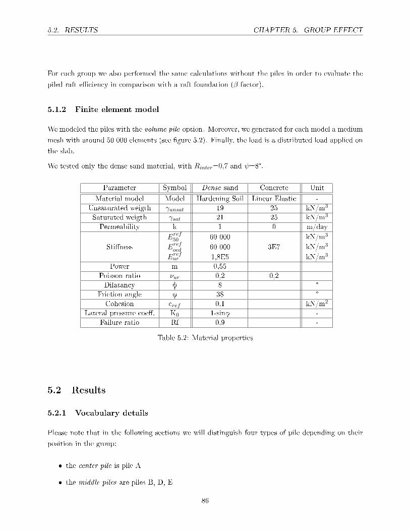
5.2. RESULTS CHAPTER 5. GROUP EFFECT
For each group we also performed the same calculations without the piles in order to evaluate the
piled raft e�ciency in comparison with a raft foundation (β-factor).
5.1.2 Finite element model
We modeled the piles with the volume pile option. Moreover, we generated for each model a medium
mesh with around 50 000 elements (see �gure 5.2). Finally, the load is a distributed load applied on
the slab.
We tested only the dense sand material, with Rinter=0,7 and ψ=8°.
Parameter Symbol Dense sand Concrete Unit
Material model Model Hardening Soil Linear Elastic -
Unsaturated weigth γunsat 19 25 kN/m3
Saturated weigth γsat 21 25 kN/m3
Permeability k 1 0 m/day
Eref50 60 000 kN/m3
Sti�ness Erefoed 60 000 3E7 kN/m3
Erefur 1,8E5 kN/m3
Power m 0,55
Poisson ratio νur 0,2 0,2 -
Dilatancy y 8 °
Friction angle f 38 °
Cohesion cref 0,1 kN/m2
Lateral pressure coe�. K0 1-sinf -
Failure ratio Rf 0,9 -
Table 5.2: Material properties
5.2 Results
5.2.1 Vocabulary details
Please note that in the following sections we will distinguish four types of pile depending on their
position in the group:
� the center pile is pile A
� the middle piles are piles B, D, E
86
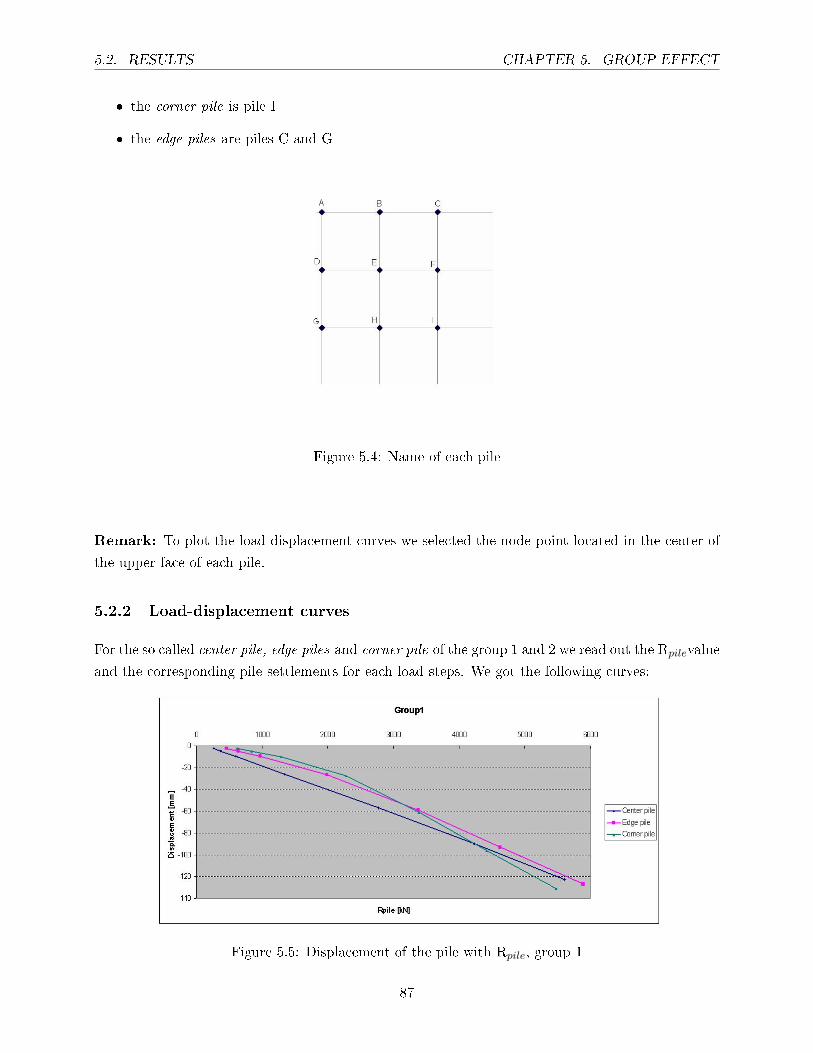
5.2. RESULTS CHAPTER 5. GROUP EFFECT
� the corner pile is pile I
� the edge piles are piles C and G
Figure 5.4: Name of each pile
Remark: To plot the load displacement curves we selected the node point located in the center of
the upper face of each pile.
5.2.2 Load-displacement curves
For the so called center pile, edge piles and corner pile of the group 1 and 2 we read out the Rpilevalue
and the corresponding pile settlements for each load steps. We got the following curves:
Figure 5.5: Displacement of the pile with Rpile, group 1
87
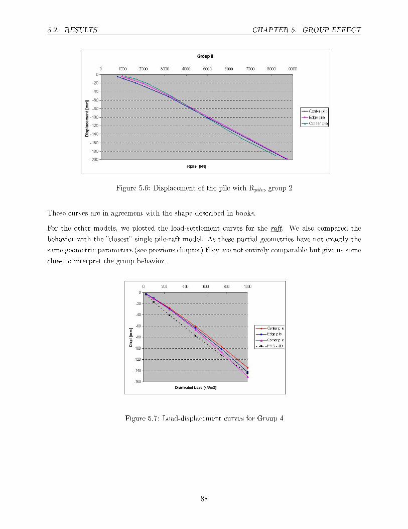
5.2. RESULTS CHAPTER 5. GROUP EFFECT
Figure 5.6: Displacement of the pile with Rpile, group 2
These curves are in agreement with the shape described in books.
For the other models, we plotted the load-settlement curves for the raft. We also compared the
behavior with the �closest� single pile-raft model. As these partial geometries have not exactly the
same geometric parameters (see previous chapter) they are not entirely comparable but give us some
clues to interpret the group behavior.
Figure 5.7: Load-displacement curves for Group 4
88
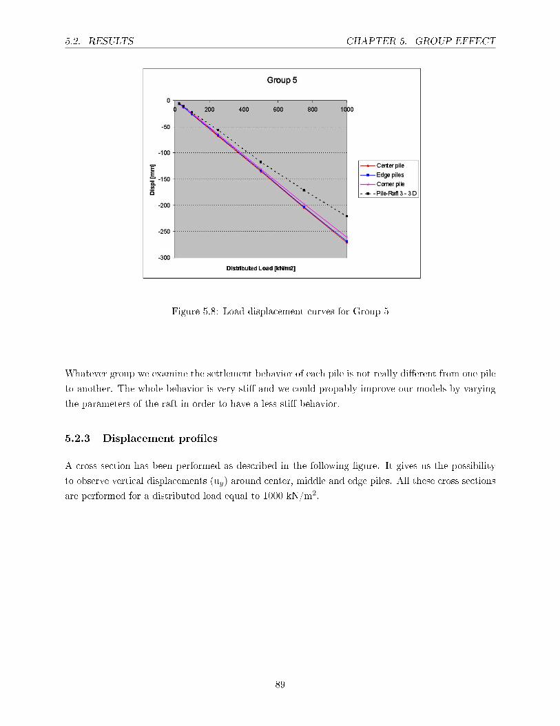
5.2. RESULTS CHAPTER 5. GROUP EFFECT
Figure 5.8: Load-displacement curves for Group 5
Whatever group we examine the settlement behavior of each pile is not really di�erent from one pile
to another. The whole behavior is very sti� and we could propably improve our models by varying
the parameters of the raft in order to have a less sti� behavior.
5.2.3 Displacement pro�les
A cross section has been performed as described in the following �gure. It gives us the possibility
to observe vertical displacements (uy) around center, middle and edge piles. All these cross sections
are performed for a distributed load equal to 1000 kN/m2.
89
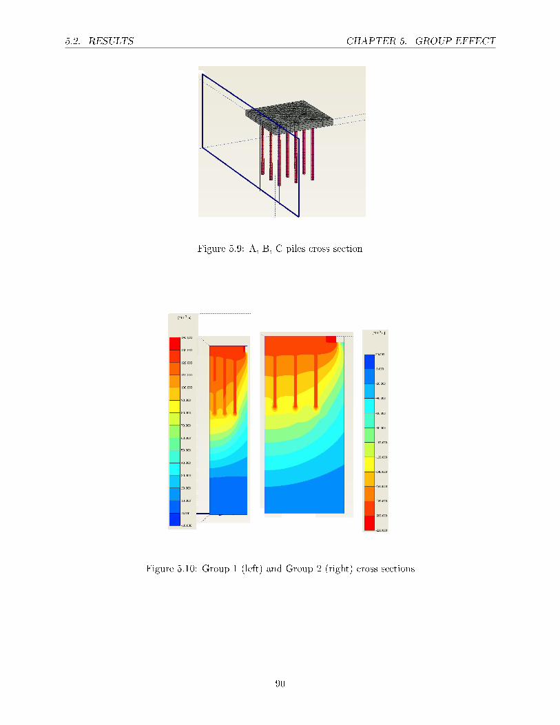
5.2. RESULTS CHAPTER 5. GROUP EFFECT
Figure 5.9: A, B, C piles cross section
Figure 5.10: Group 1 (left) and Group 2 (right) cross sections
90
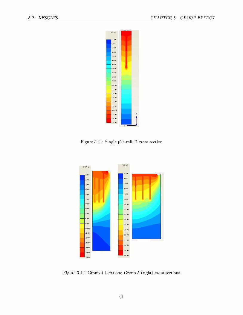
5.2. RESULTS CHAPTER 5. GROUP EFFECT
Figure 5.11: Single pile-raft II cross section
Figure 5.12: Group 4 (left) and Group 5 (right) cross sections
91
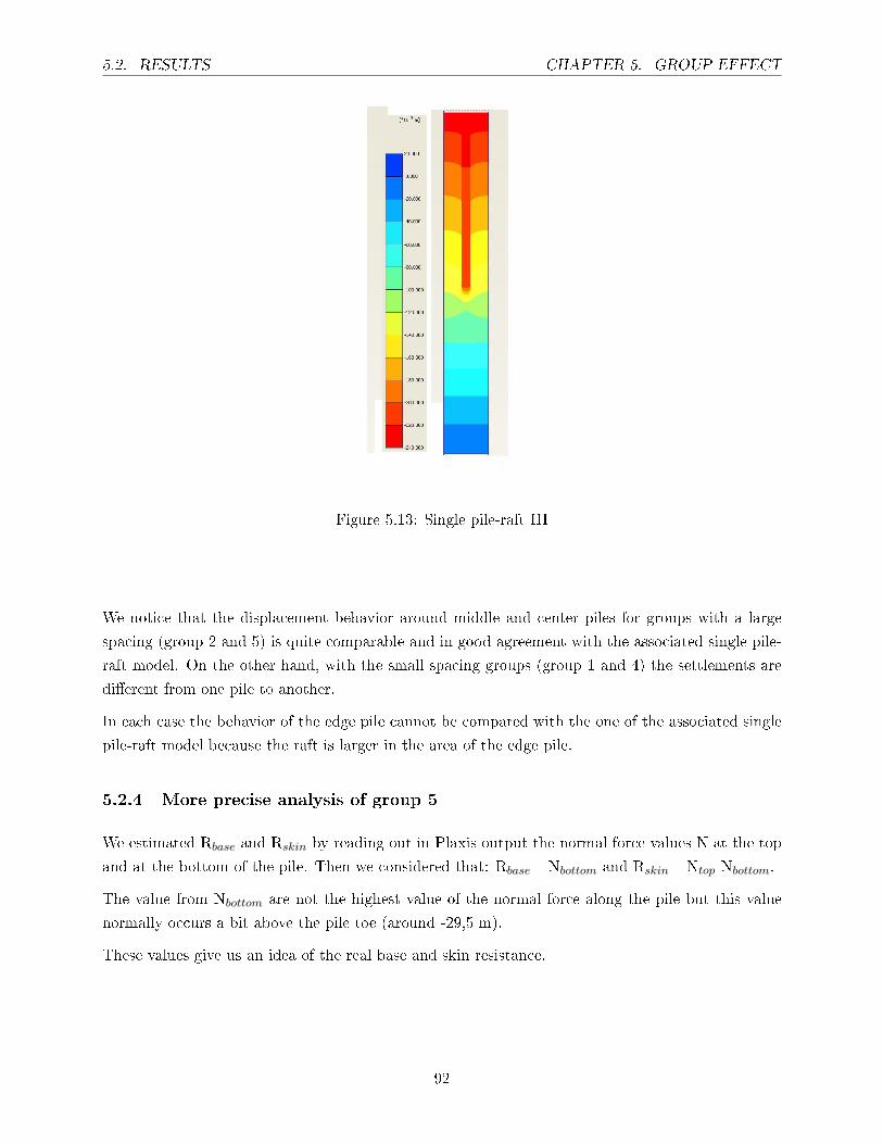
5.2. RESULTS CHAPTER 5. GROUP EFFECT
Figure 5.13: Single pile-raft III
We notice that the displacement behavior around middle and center piles for groups with a large
spacing (group 2 and 5) is quite comparable and in good agreement with the associated single pile-
raft model. On the other hand, with the small spacing groups (group 1 and 4) the settlements are
di�erent from one pile to another.
In each case the behavior of the edge pile cannot be compared with the one of the associated single
pile-raft model because the raft is larger in the area of the edge pile.
5.2.4 More precise analysis of group 5
We estimated Rbase and Rskin by reading out in Plaxis output the normal force values N at the top
and at the bottom of the pile. Then we considered that: Rbase= Nbottom and Rskin= Ntop-Nbottom.
The value from Nbottom are not the highest value of the normal force along the pile but this value
normally occurs a bit above the pile toe (around -29,5 m).
These values give us an idea of the real base and skin resistance.
92
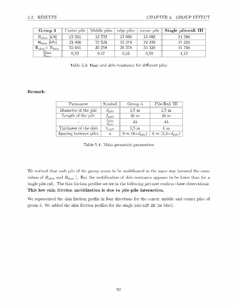
5.2. RESULTS CHAPTER 5. GROUP EFFECT
Group 5 Center pile Middle piles edge piles corner pile Single pile-raft III
Rskin [kN] 12 281 12 732 13 060 13 092 24 268
Rbase [kN] 23 400 22 526 23 318 22 228 21 500
Rskin+ Rbase 35 681 35 258 36 378 35 320 45 768Rskin
Rbase0,52 0,57 0,56 0,59 1,12
Table 5.3: Base and skin resistance for di�erent piles
Remark:
Paramater Symbol Group 5 Pile-Raft III
Diameter of the pile dpile 1,5 m 1,5 m
Length of the pile Lpile 30 m 30 m
-Lpile
dpile45 45
Thickness of the slab traft 1,5 m 1 m
Spacing between piles a 9 m (6×dpile) 8 m (5,3×dpile)
Table 5.4: Main geometric parameters
We noticed that each pile of the group seems to be mobilizated in the same way (around the same
values of Rskin and Rbase ). But the mobilization of skin resistance appears to be lower than for a
single pile-raft. The skin friction pro�les we see in the following pictures con�rm these observations.
This low skin friction mobilization is due to pile-pile interaction.
We represented the skin friction pro�le in four directions for the center, middle and corner piles of
group 5. We added the skin friction pro�les for the single pile-raft III (in blue).
93
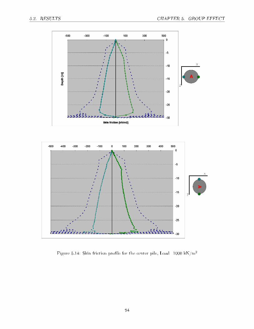
5.2. RESULTS CHAPTER 5. GROUP EFFECT
Figure 5.14: Skin friction pro�le for the center pile, Load=1000 kN/m2
94
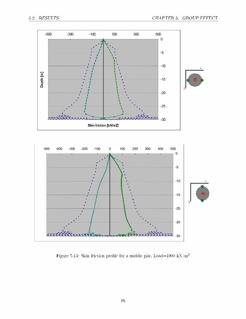
5.2. RESULTS CHAPTER 5. GROUP EFFECT
Figure 5.15: Skin friction pro�le for a middle pile, Load=1000 kN/m2
95
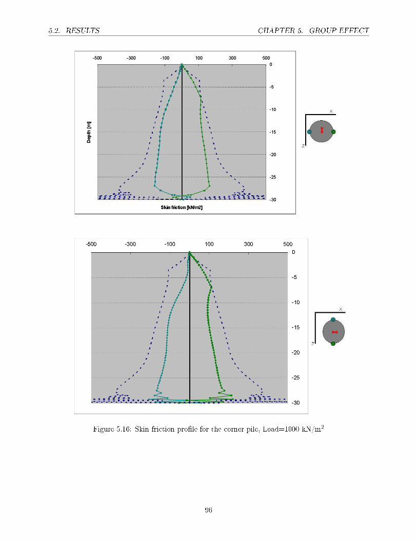
5.2. RESULTS CHAPTER 5. GROUP EFFECT
Figure 5.16: Skin friction pro�le for the corner pile, Load=1000 kN/m2
96
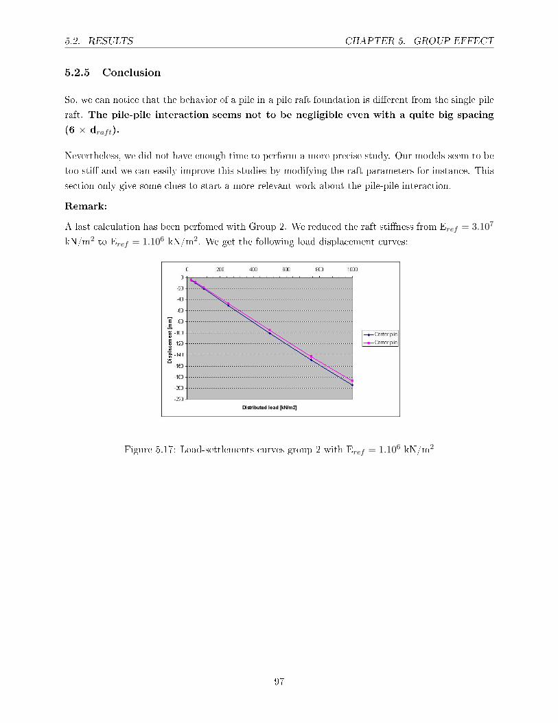
5.2. RESULTS CHAPTER 5. GROUP EFFECT
5.2.5 Conclusion
So, we can notice that the behavior of a pile in a pile raft foundation is di�erent from the single pile
raft. The pile-pile interaction seems not to be negligible even with a quite big spacing
(6 × draft).
Nevertheless, we did not have enough time to perform a more precise study. Our models seem to be
too sti� and we can easily improve this studies by modifying the raft parameters for instance. This
section only give some clues to start a more relevant work about the pile-pile interaction.
Remark:
A last calculation has been perfomed with Group 2. We reduced the raft sti�ness from Eref = 3.107
kN/m2 to Eref = 1.106 kN/m2. We get the following load displacement curves:
Figure 5.17: Load-settlements curves group 2 with Eref = 1.106 kN/m2
97
Chapter 6
Conclusion
This work led us to both practical and more general conclusions.
In chapter 2 a parametric study has been performed. Some remarks about how to design axisym-
metric single pile or pile-raft models with Plaxis can be done.
For a single pile:
� The importance of interface elements was shown. The input value for Rinter changes the load
settlement curves
� The mesh dependency is negligible
� Prescribed displacement seems to be better than load control to study a single pile
� By using load control, premature failures can occur. We can prevent this problem switching
arc-length control o�. But without arc-length control, oscillations can appear. We observed
we have to interpret with caution the shape of these �numerical inacuracies�.
For a single pile-raft:
� The mesh dependency is negligible
� The input value for Rinter do not have an important in�uence
� Dilatancy do not have an important in�uence
In chapter 4 we tested some 3D Plaxis tools to model piles: volume pile and embedded pile. The
results observed with volume piles are in a very good agreement with the ones of axisymmetric
models. On the other hand, the use of embedded pile to model piled-raft foundations was more
di�cult. We did not manage to calculate the pile raft behavior we had observed with
98
CHAPTER 6. CONCLUSION
volume piles or axisymmetric models. The main problem remains the mobilization of
the base resistance because whatever the input is, we underestimate Rbase with embedded piles
in comparison with 2D models.
Chapter 3 and 5 were focused on the analysis of the load repartition in piled-raft foundations. The
ability of Plaxis to model the complex pile-raft-soil interaction was con�rmed. We observed the
main aspects of the pile-raft behavior that are usually described in books. We noticed
that:
� The stress repartition between the raft and the pile evolves with the loading. The higher the
loading is, the more the stress is shared. With a load between 0 and 200 kN/m2 everything
goes mostly to the pile (1 <αKpp< 0,8). From 200 kN/m2the raft has a stronger in�uence.
� The bigger the spacing is, the more load takes the raft.
� In each case the raft and pile load sharing converges to an equilibrium state
� The pile obviously carries more load by increasing the length of the pile
We started a more sophisticated analysis of the total structure with a three dimensional model to
take the pile-pile interactions into account. We noticed that the behavior of a pile in a piled raft
foundation is di�erent from the single pile raft model. There is a reduction of the skin friction
mobilization due to a group e�ect. We did not have enougth time left to pursue in more details
the improvement of these models. This �nal chapter gives some basic clues to perform a deeper
analysis of pile-pile interactions in piled-raft foundations. This e�ect should be studied in further
researches.
99
Bibliography
[1] Brinkgreve R.B.J (2006). Plaxis, Finite Element Code for Soil and Rock Analyses, user
manual. Delft University of Technology & Plaxis b.v, The Nederlands. Balkema, Rotterdam.
[2] Y. El-Mossalany. Single pile and pile group in overconsolidated clay, Plaxis 3D foundation /
validation Version 2. Ain shams University
[3] Y. El-Mossalany. Pile raft foundation in frankfurter clay, Plaxis 3D foundation / validation
Version 2. Ain Shams University
[4] H. K Engin. Validation of embedded piles, the Azley Bridge pile load test, Plaxis 3D foundation
/ validation Version 2. Middle-East Technical University
[5] F. Tschuchnigg and H. Schweiger. Application of the ground anchor facility, Plaxis 3D
foundation / validation Version 2. Graz University of Technology
[6] M. Wehnert and P.A. Vermeer. Numerical Analyses of Load Tests on Bored Piles. University
of Stuttgart
100


