
394
American Economic Review 2010, 100:1, 394–419http://www.aeaweb.org/articles.php?doi=10.1257/aer.100.1.394
The General Agreement on Tariffs and Trade (GATT) and the World Trade Organization (WTO) more generally, like all existing trade agreements, are obviously highly incomplete con-tracts. In the economics literature there exist models of trade agreements as incomplete contracts, but the typical approach is to impose exogenous restrictions on the set of policy instruments that can be included in the agreement, and examine what the agreement can accomplish given these limitations.1 This literature illuminates the consequences of the incompleteness of trade agree-ments, but it cannot explain the particular forms that the incompleteness has taken.
The broad purpose of this paper is to take the analysis of trade agreements as incomplete con-tracts one step further, by endogenously determining the choice of contract form. A more spe-cific purpose is to argue that an incomplete-contracting perspective can help explain three core features of the GATT/WTO. (i) The agreement binds the levels of trade instruments. In contrast, domestic instruments are largely left to the discretion of governments, with two important excep-tions: first, internal policies must be nondiscriminatory according to the National Treatment (NT) clause; and, second, the WTO has introduced a regulation of domestic subsidies. (ii) The bindings are largely rigid (i.e., not state contingent). But there are “escape clauses” that allow for temporary protection. (iii) The bindings stipulate only upper bounds on the tariffs, thus leaving governments with discretion to go below the bounds.
An important property of the incompleteness of the GATT/WTO, which is embodied in the features above, is that the agreement displays an interesting combination of rigidity, in the sense that contractual obligations are largely insensitive to changes in economic (and political) con-ditions, and discretion, in the sense that governments have substantial leeway in the setting of many policies. This property is also exhibited to varying degrees by all other existing trade
1 An incomplete list of papers that fall into this category is Brian R. Copeland (1990), Kyle Bagwell and Staiger (2001), Pierpalo Battigalli and Maggi (2003), Horn (2006) and Arnaud Costinot (2008).
Trade Agreements as Endogenously Incomplete Contracts
By Henrik Horn, Giovanni Maggi, and Robert W. Staiger*
We propose a model of trade agreements in which contracting is costly, and as a consequence the optimal agreement may be incomplete. In spite of its sim-plicity, the model yields rich predictions on the structure of the optimal trade agreement and how this depends on the fundamentals of the contracting envi-ronment. We argue that taking contracting costs explicitly into account can help explain a number of key features of real trade agreements. (JEL D86, F13)
* Horn: Research Institute of Industrial Economics, Box 55665, SE-102 15 Stockholm, Sweden, Bruegel, and CEPR (e-mail: [email protected]); Maggi: Department of Economics, Yale University, New Haven, CT 06520, NBER, and CEPR (e-mail: [email protected]); Staiger: Department of Economics, Stanford University, 579 Serra Mall, Stanford, CA 94305, and NBER (e-mail: [email protected]). This paper has benefited from the detailed and help-ful comments of three referees, as well as from the helpful comments of Kyle Bagwell, Pierpaolo Battigalli, Gene Grossman, Elhanan Helpman, Robert Lawrence, Andres Rodriguez-Clare, Johan Stennek, and seminar participants at the University of Calgary, CEMFI, Ente Luigi Einaudi, Harvard Univerity, Minneapolis Federal Reserve, Penn State University, Princeton University, UBC, UC Davis, UCSD, and Yale University, and from participants in ERWIT, ETSG, and CREI (Universitat Pompeu Fabra) conferences. Horn gratefully acknowledges financial support from the Marianne and Marcus Wallenberg Foundation. Maggi gratefully acknowledges financial support from the NSF (grant SES-0351586) and thanks the Ente Luigi Einaudi for hospitality during part of this project. Staiger gratefully acknowl-edges financial support from the NSF (grant SES-0518802).

VOL. 100 NO. 1 395HORN Et AL.: ENdOgENOusLy INcOmpLEtE cONtRActs
agreements. In this paper we propose a simple theoretical framework where the manner and degree in which discretion and rigidity are present in the agreement is optimally determined.
We assume that governments face two fundamental challenges when designing a trade agree-ment. The first is that there is a wide array of policy instruments—border measures and espe-cially “domestic” measures—that should be constrained to keep in check each government’s incentives to act opportunistically. This feature suggests that the agreement should be com-prehensive in its policy coverage. The second is that there is significant uncertainty about the circumstances that will prevail during the lifetime of the agreement. This feature suggests that the agreement should be highly state contingent. These features would not pose a problem if contracting were costless. But in reality there are important costs of negotiating and drafting a trade agreement. These costs are likely to be higher when the agreement is more detailed, both in terms of the policies that it seeks to constrain and the contingencies that it specifies. We explicitly incorporate the costs of contracting over policies and contingencies into our model.2
We work within a competitive two-country setting, where both consumption and production may create (localized) externalities, thereby giving rise to multiple possible rationales for policy intervention. We focus on intervention in import sectors, and assume that governments possess a complete set of tax instruments. We look first at tariffs and production subsidies, but later also consider consumption taxes in order to evaluate the NT clause. Uncertainty plays a central role. To bring out the main points, we consider three sources of uncertainty: the consumption exter-nality, the production externality, and the underlying trade volume.
In the absence of an agreement, the importing country would use its policies to correct the externalities, but it would also use its tariff to manipulate the terms of trade. This would lead to a globally inefficient outcome, and hence there is scope for an agreement to restrain governments from behaving opportunistically. Were it not for the externalities, the first-best agreement would be very simple: it would stipulate a blanket laissez-faire rule. But due to the externalities, the con-tracting problem is more complex: the first-best agreement involves state-contingent constraints on all policy instruments.
Following an approach similar to Battigalli and Maggi (2002), we assume that contracting costs are increasing in the number of state variables and policies included in the agreement, and we characterize the agreement that maximizes expected global welfare minus contracting costs (the “optimal” agreement). As a result of contracting costs, the optimal agreement may be sim-pler than the first-best agreement, and in particular it may feature (partial or full) rigidity and/or discretion over some of the policies.
Our first result is that it cannot be optimal to contract over domestic subsidies while leaving tariffs to discretion. This finding reflects a kind of “targeting principle” logic: contracting over subsidies alone is suboptimal because it is the tariff that is the source of the inefficiency in the noncooperative equilibrium. This finding accords well with the emphasis on trade measures that
2 An objection might be raised that the costs of contracting are likely to be small relative to the gains from a trade agreement. But one should keep in mind the vast number of products, countries, policy instruments, and contingencies that are involved in such an agreement. Indeed, the WTO agreement, despite its obvious incompleteness, still fills some 24,000 pages and took approximately 8 years of negotiations to complete. Hence, we believe it is reasonable to view the contracting costs of trade agreements as substantial. This view is shared by many trade-law scholars. For example, Robert E. Hudec (1990) writes: “The standard trade policy rules could deal with the common type of trade policy mea-sure governments usually employ to control trade. But trade can also be affected by other ‘domestic’ measures, such as product safety standards, having nothing to do with trade policy. It would have been next to impossible to catalogue all such possibilities in advance” ( p. 24). And Warren F. Schwartz and Alan O. Sykes (2002) write: “ Many contracts are negotiated under conditions of considerable complexity and uncertainty, and it is not economical for the parties to specify in advance how they ought to behave under every conceivable contingency....The parties to trade agree-ments, like the parties to private contracts, enter the bargain under conditions of uncertainty. Economic conditions may change, the strength of interest group organization may change, and so on” ( pp. 181–84).

mARcH 2010396 tHE AmERIcAN EcONOmIc REVIEW
characterizes the GATT/WTO; and while this feature is often explained informally as deriving from distinct levels of contracting costs across these instruments, our model imposes no such distinction, and so it identifies in this respect a more fundamental explanation.
The next question is whether subsidies should (also) be constrained by the agreement. The key trade-off involved in this choice is the following. A first, direct benefit of leaving subsidies to the governments’ discretion is given by the direct savings in contracting costs; but we also identify a second benefit, which applies whenever the agreement is rigid with respect to the externalities, and this is the indirect state contingency accomplished when subsidies are discretionary. The cost of leaving subsidies to discretion takes the form of distortions in the subsidy for terms-of-trade manipulation: we identify monopoly power, trade volume, and instrument substitutability effects as key features of the contracting environment that determine the severity of these distor-tions and hence the costs of discretion. Using these effects, our second result is that it is optimal to leave subsidies to discretion if: (i) countries have little monopoly power in trade, in which case they have little ability to manipulate terms of trade; (ii) they trade little, in which case they gain little from exploiting their power over terms of trade; or (iii) subsidies are a poor substitute for tariffs as a tool for manipulating the terms of trade.
The trade volume effect identified above suggests a possible explanation for the fact that the WTO has introduced a regulation of domestic subsidies that was not present in GATT, namely that a general increase in trade volumes over time has increased the cost of discretion, thereby heightening the need to constrain domestic policies. And in combination with the monopoly power and instrument substitutability effect, the model also suggests a reason why developing countries were largely exempted from the WTO regulation of subsidies through “special and dif-ferential treatment” clauses: the typical developing country may lack both the market power and the array of domestic policy instruments to find easy substitutes for tariffs.
We next examine whether the optimal agreement is state contingent and, if so, what state variables should be included. The cost of including a state variable must be weighed against the benefit of doing so, and the latter is in turn largely determined by the degree of uncertainty over the externalities. But whenever the agreement leaves subsidies to discretion, there is also a more subtle insight concerning why contingent tariff commitments may be beneficial, and which con-tingencies to specify. Since the incentive to distort subsidies for terms-of-trade purposes grows with the underlying trade volume, making tariffs state contingent can help mitigate this incen-tive against especially high trade volumes. We label this the indirect incentive management effect. This effect is at the core of our third result: conditional on leaving subsidies to discretion, it can be optimal to make tariffs contingent on state variables that affect the trade volume but are irrelevant to the first-best tariff level. An implication of this result is that it can be optimal to specify an escape clause–type rule that allows governments to raise tariffs when the level of import demand is high, as a way to manage the higher incentives to distort domestic instruments for terms-of-trade purposes in periods of high underlying import volume.
Next, we extend the model to shed light on two other core aspects of the GATT/WTO: the presence of an NT clause, and the fact that tariffs are constrained by “weak” bindings (i.e., upper bounds) rather than by “strong” bindings (i.e., exact levels).
We evaluate the NT clause as a means of saving on contracting costs. To this end, we allow for distinct consumption taxes on domestically produced and imported goods, and we interpret the NT clause as requiring that these consumption taxes be equalized. We first show that an agree-ment that includes the NT clause but does not bind the consumption tax offers a novel form of discretion that cannot be achieved without the NT clause, namely discretion over the consumer price wedge (a non-NT agreement can leave discretion only over the producer price wedge). We then derive a simple condition for the optimal agreement to feature this form of discretion and hence to include the NT clause. This condition describes circumstances in which an NT-based

VOL. 100 NO. 1 397HORN Et AL.: ENdOgENOusLy INcOmpLEtE cONtRActs
agreement is attractive because it economizes on costly state-contingencies, by using, instead, the indirect state-contingency associated with discretion over internal taxes.
Finally, we argue that the presence of contracting costs may explain why GATT stipulates weak bindings rather than strong bindings. More specifically, we show that the optimal agree-ment may include rigid weak bindings. The appeal of this type of binding is that it combines rigidity and discretion in a novel fashion, since the ceiling does not depend on the state of the world, and the government has (downward) discretion to set the policy below the ceiling.
The paper is organized as follows. Section I lays out the basic model and characterizes the optimal agreement. Section II examines the role of the NT clause. Section III examines the role of weak bindings. Section IV concludes. The Appendix provides proofs not contained in the body of the paper.
I. The Basic Model
We consider two countries, Home and Foreign. There are three goods, a numeraire good (which is freely traded) and two nonnumeraire goods (labeled 1 and 2). Home is a natural importer of good 1 and Foreign a natural importer of good 2. Markets are perfectly competitive, but we allow for the presence of a production externality and a consumption externality, thus giving rise to multiple economic rationales for policy intervention.
We start by describing the supply structure in the Home country. The numeraire good is pro-duced one for one from labor, with the supply of labor large enough to ensure strictly positive production; therefore the equilibrium wage is equal to one. Each nonnumeraire good j ∈ {1, 2} is produced from labor according to the concave production function Xj = fj (L j ) with fj′ > 0 and fj″ < 0, where X j is the production of good j and L j is the labor employed in the production of good j. With q j denoting the producer price for good j and with the wage fixed at one, the supply and profit functions for good j can then be expressed as increasing functions of q j, and we denote these functions by X j (q j ) and Π j (q j ), respectively. We assume a similar supply structure for the Foreign country, and let asterisks denote Foreign variables: X j* = fj
*(L j* ) with f *′j > 0 and f *″j < 0, with associated supply and profit functions given by X j*(qj
* ) and Π j*(qj* ), respectively.
As noted above, we allow for the possibility of a (positive) production externality. We assume that the externality is linear in aggregate domestic production, enters directly and separably into the representative citizen’s utility, and does not cross borders. Producers ignore the effects of their production on the level of aggregate production, and the externality does not affect supply functions (see James R. Markusen (1975) and Josh Ederington (2001) for analogous represen-tations of production externalities). Also, we assume that the production of good 1 generates an externality only in Home, and good 2 only in Foreign. Hence, the value of the production externality in Home is σ1X1, while in Foreign it is σ2
* X2*, with the parameters σ1 and σ2
* (defined positively) capturing the strength of the production externality in each country.3
In each country, the representative citizen’s utility function is linear in the numeraire good and separable in the nonnumeraire goods. We also allow for the possibility of a (negative) consump-tion externality. In analogy with the production externality described above, we assume that the consumption externality is linear in aggregate domestic consumption and does not cross borders. Also, as with the production externality, we assume that consumption of good 1 generates an externality only in Home, and good 2 only in Foreign.
Formally, the representative citizens of the two countries enjoy the following utility:
3 The assumption that externalities are experienced only by the importing country does not play a critical role in our results, but seems natural in light of the focus on import-sector intervention that we introduce below.

mARcH 2010398 tHE AmERIcAN EcONOmIc REVIEW
u = c0 + ∑ j=1
2
uj (cj ) − γ1c1 + σ1X1 and u * = c0* + ∑
j=1
2
uj* (cj
* ) − γ2* c2
* + σ*2 X *
2,
where cj and cj denote, respectively, individual and aggregate consumption of good j. The param-eters γ1 and γ2
* (defined positively) capture the strength of the consumption externality in each country. Consumers ignore the effects of their individual consumption on aggregate consump-tion, so the externality does not affect demand functions. We assume that the subutility functions are concave, so that the implied Home and Foreign demands are decreasing functions of the Home and Foreign consumer prices pj and pj
*, respectively. We let dj( pj ) and dj* ( pj
* ) denote the Home and Foreign demands. Assuming that the population in each country is a continuum of measure 1, the consumer surplus associated with good j in Home and Foreign, respectively, is Γj( pj) = uj (dj ( pj )) − pj dj( pj ) and Γj
* ( pj*) = uj
* (dj* ( pj
* )) − pj*dj
*( pj* ).
We assume that each government can intervene only in its import sector, but within this sector we allow each government to use a pair of instruments, namely, a specific import tariff (τ) and a specific domestic production subsidy (s). We will also introduce consumption taxes in Section II, when we consider the rationale for the NT clause. We note, though, that τ and s together already comprise a complete set of taxes for the import sector.
At this point we impose a strong symmetric structure on the model: we assume that the two nonnumeraire sectors are mirror images of each other. This allows us to focus on a single sector and drop subscripts from now on. We focus on sector 1, where Home is the natural importer, but it should be kept in mind that in the background there is a mirror-image sector with identical equilibrium conditions, except that the two countries’ roles are reversed. The symmetry of the model is inessential, and could be relaxed at the cost of extra notation.
Throughout the paper we focus on nonprohibitive levels of government intervention. In the sector under consideration, due to the absence of taxation by the Foreign government, Foreign producer and consumer prices are equalized, or q* = p*. In addition, for a firm in Foreign to sell in both countries, it must receive the same price for sales in Foreign that it receives after taxes for sales in Home, or p* = p − τ. And, finally, the relationship between the Home producer price and the Home consumer price is given by q = p + s.
We can express the pricing relationships above in more compact form as
(1) p = p* + τ and
q = p* + τ + s.
The arbitrage relationships in (1) describe the two central price wedges in the model: the first is the wedge between the Home consumer price and the Foreign price (equal to τ ), and the second is the wedge between the Home producer price and the Foreign price (equal to τ + s ).4
Market clearing requires that world demand equal world supply, or
(2) d( p) + d*( p* ) = X (q) + X *(q* ).
The market clearing condition (2), together with the two arbitrage relationships in (1), deter-mines the three market clearing prices as functions of τ and s: p(τ, s), q(τ, s), and p*(τ, s). At the market clearing prices, Home import volume, m ≡ d − X, is equal to Foreign export volume,
4 The relationships in (1) also confirm that τ and s together comprise a complete set of taxes for the import sector: as is well known, an import tariff acts as both a tax on consumption and a subsidy to producers of the import-competing good, and together with a production subsidy the consumer and producer margins can be independently targeted with the two instruments.

VOL. 100 NO. 1 399HORN Et AL.: ENdOgENOusLy INcOmpLEtE cONtRActs
E * ≡ X * − d*. Finally, using p(τ, s), q(τ, s), and p*(τ, s), we can also define economic magnitudes directly as functions of policies. With a slight abuse of notation, we define:
d(τ, s) ≡ d( p(τ, s)), X(τ, s) ≡ X(q(τ, s)), m(τ, s) ≡ d(τ, s) − X(τ, s),
Γ(τ, s) ≡ Γ( p(τ, s)), and Π(τ, s) ≡ Π(q(τ, s));
and similarly for the Foreign country:
d*(τ, s) ≡ d*( p*(τ, s)), X *(τ, s) ≡ X *( p*(τ, s)), E*(τ, s) ≡ X *(τ, s) − d*(τ, s),
Γ*(τ, s) ≡ Γ*( p*(τ, s)), and Π*(τ, s) ≡ Π *( p*(τ, s)).
Note that m(0, 0) > 0 under our assumption that the Home country is a natural importer of the good under consideration.
We assume that each government maximizes the welfare of its representative citizen. Since the welfare function is separable across sectors, we can focus again on sector 1. In this sector, Home welfare can be written as the sum of consumer surplus, profits, net revenue (i.e., revenue from the import tariff τ minus expenditures on the production subsidy s), and the valuation of the externalities. Therefore, we can write the Home government’s objective as
W(τ, s) ≡ Γ (τ, s) + Π (τ, s) + τ m(τ, s) − sX (τ, s) + σ X(τ, s) − γ d(τ, s).
Recalling that in the sector under consideration the Foreign country has no externalities and no policy instruments of its own, Foreign welfare is the sum of consumer surplus and profits:
W *(τ, s) ≡ Γ*(τ, s) + Π *(τ, s).
Notice that, as can be confirmed from the definitions of Γ*(τ, s) and Π *(τ, s), Home’s policies affect Foreign welfare only through the terms of trade p*.
A. the Efficient policies and the Noncooperative Equilibrium
We first derive the globally efficient policies, which we define as the policies that maximize the sum of Home and Foreign payoffs:5
W g(τ, s) ≡ W (τ, s) + W *(τ, s).
We assume that both W (τ, s) and W g(τ, s) are concave in τ and s. It is direct to verify that the efficient levels of τ and s, which we denote by τ eff and s eff, are, respectively, given by
(3) τ eff = γ and
s eff = σ − γ.
5 In our symmetric setting, it is natural to define efficiency in this way. Recall that there is another sector that mirrors exactly the one under consideration, and in which Foreign is the importer. Therefore, a combination of policies that is Pareto-efficient and gives the same welfare to the two countries must maximize the sum of Home and Foreign payoffs in each sector. This notion of efficiency would also be appropriate in asymmetric settings, provided that international lump-sum transfers were available.
mARcH 2010400 tHE AmERIcAN EcONOmIc REVIEW
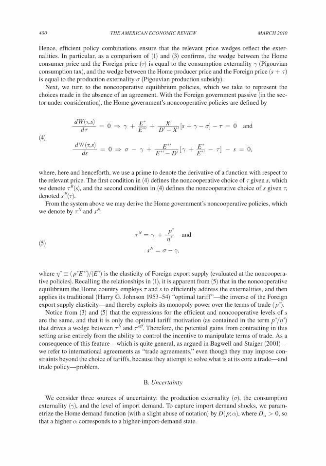
Hence, efficient policy combinations ensure that the relevant price wedges reflect the exter-nalities. In particular, as a comparison of (1) and (3) confirms, the wedge between the Home consumer price and the Foreign price (τ) is equal to the consumption externality γ (Pigouvian consumption tax), and the wedge between the Home producer price and the Foreign price (s + τ) is equal to the production externality σ (Pigouvian production subsidy).
Next, we turn to the noncooperative equilibrium policies, which we take to represent the choices made in the absence of an agreement. With the Foreign government passive (in the sec-tor under consideration), the Home government’s noncooperative policies are defined by
(4)
d W (τ, s) _______
d τ = 0 ⇒ γ + E * ___ E *′ + X ′ ______
d′ − X ′ [s + γ − σ] − τ = 0 and
d W (τ, s) _______
ds = 0 ⇒ σ − γ + E *′ _______
E *′ − d′ [ γ + E * ___ E *′ − τ ] − s = 0,
where, here and henceforth, we use a prime to denote the derivative of a function with respect to the relevant price. The first condition in (4) defines the noncooperative choice of τ given s, which we denote τ R(s), and the second condition in (4) defines the noncooperative choice of s given τ, denoted s R(τ).
From the system above we may derive the Home government’s noncooperative policies, which we denote by τ N and s N:
(5) τ N = γ + p
*
___ η* and
s N = σ − γ,
where η* ≡ ( p*E *′)/(E *) is the elasticity of Foreign export supply (evaluated at the noncoopera-tive policies). Recalling the relationships in (1), it is apparent from (5) that in the noncooperative equilibrium the Home country employs τ and s to efficiently address the externalities, and then applies its traditional (Harry G. Johnson 1953–54) “optimal tariff”—the inverse of the Foreign export supply elasticity—and thereby exploits its monopoly power over the terms of trade ( p*).
Notice from (3) and (5) that the expressions for the efficient and noncooperative levels of s are the same, and that it is only the optimal tariff motivation (as contained in the term p*/η*) that drives a wedge between τ N and τ eff. Therefore, the potential gains from contracting in this setting arise entirely from the ability to control the incentive to manipulate terms of trade. As a consequence of this feature—which is quite general, as argued in Bagwell and Staiger (2001)—we refer to international agreements as “trade agreements,” even though they may impose con-straints beyond the choice of tariffs, because they attempt to solve what is at its core a trade—and trade policy—problem.
B. uncertainty
We consider three sources of uncertainty: the production externality (σ), the consumption externality (γ), and the level of import demand. To capture import demand shocks, we param-etrize the Home demand function (with a slight abuse of notation) by d( p; α), where dα > 0, so that a higher α corresponds to a higher-import-demand state.

VOL. 100 NO. 1 401HORN Et AL.: ENdOgENOusLy INcOmpLEtE cONtRActs
Uncertainty about σ and γ can be interpreted as uncertainty about the efficiency rationale for policy intervention, while shocks to α can be interpreted as shocks to the underlying trade vol-ume. Focusing on uncertainty in σ, γ, and α while abstracting from other sources of uncertainty helps to illustrate some general principles for understanding the nature of the optimal agreement. We sometimes refer to σ, γ, and α as the state-of-the-world variables, or simply the “state” vari-ables. Note that we do not impose any particular structure on the distribution of these variables.
We consider the following simple timing: (i) the agreement is drafted; (ii) uncertainty is resolved; and (iii) policies are chosen subject to the constraints set by the agreement. Implicit in this timing is the assumption that agreements are perfectly enforceable: in this paper we abstract from issues of self-enforcement of the agreements.
Finally, we denote expected global welfare gross of contracting costs (henceforth, simply “gross global welfare”) by Ω(·) ≡ EW g(·).
C. the costs of contracting
Before we formalize the costs of contracting, we need to specify what type of contracts we will consider. Throughout the paper we focus on instrument-based agreements, i.e., agreements that impose (possibly contingent) constraints on policy instruments. In the concluding section we briefly discuss the possibility of outcome-based agreements, i.e., agreements that impose constraints on equilibrium outcomes such as trade volumes.6
As a first step we consider a relatively narrow class of agreements, those that impose separate equality constraints on τ and s. To be concrete, we allow for clauses of the type (τ = γ) or (s = 10), but not for clauses of the type g(τ, s) = 0 or for inequality constraints of the type (τ ≤ 1).7 We label this class of agreements 0. In later sections we consider broader classes of agreements.
We formalize the contracting costs associated with a trade agreement in a very stylized way. Our central assumption is that these costs are higher, the more policy instruments the agreement involves, and the more contingencies it includes.
More specifically, we assume that there are two kinds of contracting costs: the costs of includ-ing state variables in the agreement—that is, the random variables σ, γ, and α—and the costs of including policy variables—that is, τ and s. We think of the cost of including a given variable in the agreement as capturing both the cost of describing this variable (i.e., defining the variable, how it should be measured, etc., along the lines of the “writing costs” emphasized by Battigalli and Maggi 2002) as well as the cost of verifying its value ex post.8 A broader interpretation of these contracting costs might also include negotiation costs: it is reasonable to think that negotiation costs are higher when there are more policy instruments on the table, and when there are more relevant contingencies to be discussed.
The cost of contracting over a state variable is cs, and the cost of contracting over a policy variable is cp . For simplicity, we assume that, if a variable is included in the agreement, the associated cost is incurred only once, regardless of how many times that variable is mentioned in the agreement; in other words, there is no cost of “recall.” Summarizing, the cost of writing
6 We also abstract from agreements that are based on both instruments and outcomes, such as, for example, an agree-ment that constrains τ to be a direct function of m or p*.
7 We consider agreements that impose inequality constraints of the type (τ ≤ 1) in Section III. When there is sig-nificant uncertainty, a noncontingent contract of the type g(τ, s) = 0 may do better than a noncontingent contract that pins down τ and/or s separately, because the former contract type introduces some discretion. This has the flavor of an outcome-based contract, which we discuss in the concluding section.
8 The interpretation of contracting costs as verification costs is “tight” only if the court verifies ex post the values of the variables included in the contract, at least with some probability. In the WTO, the Trade Policy Review Mechanism provides periodic reviews of the member countries’ trade policies, although a more thorough verification process in the WTO occurs only if there is a complaint by one of the contracting parties.

mARcH 2010402 tHE AmERIcAN EcONOmIc REVIEW
an agreement is c = cs ns + cp np, where ns and np are, respectively, the number of state and policy variables in the agreement. We could allow c to be a more general increasing function of ns and np, but we choose the linear specification to simplify the analysis and the exposition of our results.9
Two examples may be useful to illustrate our assumptions on contracting costs:
Example 1: The agreement {τ = 3} specifies a rigid commitment for the tariff, and costs cp.Example 2: The agreement {τ = γ, s = 5 } specifies a state-contingent commitment for the
tariff and a rigid commitment for the subsidy, and costs 2cp + cs.
Overall, our approach to modeling the costs of contracting has advantages and also limita-tions. On the plus side, our approach preserves tractability while adding some generality relative to other approaches in the literature.10 On the minus side, our approach abstracts from some potentially important considerations: for example, we assume that the number of state variables ns summarizes the costs of state-contingency, but in reality this cost might depend as well on the “coarseness” of the contingencies (e.g., it might be easier to verify a clause like (τ = 0 if γ ≤ 1) than a clause (τ = γ )). On balance, however, we believe that the basic feature that contracting costs are increasing in the number of state variables and policies included in the agreement is likely to be preserved in most reasonable models of these costs, and for this reason we believe that our approach provides a good starting point for the analysis of trade agreements as endog-enously incomplete contracts.
D. the Optimal Agreement
To characterize the optimal agreement, we need to introduce some definitions and notation. First, we refer to the efficiently-written first-best agreement as the least costly among the agree-ments that implement the first-best outcome. We label this simply the {FB} agreement. In a similar vein, we refer to the case of no agreement as the “empty agreement,” which formally is denoted {Ø}. Finally, an optimal agreement is an agreement that maximizes expected global welfare net of contracting costs (henceforth, simply “net global welfare” ), that is, ω ≡ Ω − c.11
The first step is to derive the {FB} agreement. Recall that the first-best policies are defined by (3). We can conclude that an agreement of the form {τ = γ, s = σ − γ} achieves the first-best outcome. This agreement has np = 2 and ns = 2 and therefore costs 2cp + 2cs. Moreover, it is clear that the first-best outcome cannot be implemented with an agreement that costs less than 2cp + 2cs, and so {τ = γ, s = σ − γ} is indeed the {FB} agreement in the class 0.
The {FB} agreement yields net global welfare equal to ΩFB − (2cp + 2cs ), where ΩFB denotes the gross global welfare implied by the first-best policies. Clearly, when contracting costs are sufficiently small, the {FB} agreement is optimal. We record this benchmark result with:
9 Also, as will become clear below, assuming that it is more costly to contract over internal measures (s) than over tariffs (τ) would only strengthen our qualitative results.
10 For example, Battigalli and Maggi (2002) associate a cost c with each “primitive sentence” included in the con-tract, and the analogue in our setting would be to associate a cost c with each state variable or policy included in the contract. Under this analogy, the form of contracting costs adopted by Battigalli and Maggi is a special case of our approach, in which cs = cp.
11 Our focus on the agreement that maximizes net global welfare can be justified as the equilibrium outcome of a bargaining game in a variety of ways. For example, if one government makes a take-it-or-leave-it offer incurring the associated writing costs, and if international transfers are available, the equilibrium outcome will be our optimal agree-ment. Alternatively, this would be the case if governments negotiate orally over the agreement in an efficient way (e.g., Nash bargaining), and writing costs are incurred once agreement is reached. This alternative interpretation is valid even in the absence of international transfers if the bargaining setting is symmetric (see also note 5).

VOL. 100 NO. 1 403HORN Et AL.: ENdOgENOusLy INcOmpLEtE cONtRActs
REMARK 1: If cs and cp are sufficiently low, the optimal agreement is {τ = γ, s = σ − γ}.
At the opposite extreme, if cs and cp are sufficiently high, the empty agreement (which costs nothing and yields the noncooperative equilibrium outcome) is optimal. The interesting question is what happens between these two extremes: what is the optimal way to save on contracting costs?
It is useful at this point to recall the distinction, introduced by Battigalli and Maggi (2002), between two forms of contractual incompleteness: rigidity, which occurs when state variables are missing from the agreement; and discretion, which occurs when policy variables are missing from the agreement. Thus, for example, the agreement {τ = 0, s = 5 } is fully rigid; the agree-ment {s = g (σ, γ, α)} features discretion over τ; and the agreement {τ = 3} is both rigid and dis-cretionary (over s).12 With these notions of rigidity and discretion, the question we posed above can be rephrased as: what is the optimal combination of rigidity and discretion?
Given that we have two policy variables (τ and s) and three state variables (σ, γ, and α), in principle there are many types of contract that we should consider. For this reason, it is diffi-cult to fully characterize the optimal contract without imposing more structure on the problem. Nonetheless, we are able in this general setting to derive a number of insights about the nature of the optimal agreement.13
Our first result (proved in the Appendix) is that, if an agreement is to achieve any improvement over the noncooperative equilibrium, it must constrain import taxes. More formally:
PROPOSITION 1: An agreement that constrains the subsidy s (even in a state-contingent way) while leaving the import tariff τ to discretion cannot improve over the noncooperative equilib-rium, and therefore cannot be an optimal agreement.
At a broad level, the intuition behind Proposition 1 is very simple, and reflects a kind of “tar-geting principle” logic (Jagdish Bhagwati and V. K. Ramaswami 1963; Johnson 1965): contract-ing over s alone is suboptimal because, as we have emphasized in Section IA, the inefficiency in the noncooperative equilibrium concerns τ, not s.
To develop a more precise understanding of this result, consider an agreement that imposes a small exogenous change in s starting from the noncooperative equilibrium. This triggers a change in the Home government’s choice of τ, and in particular, as we show in the Appendix, τ adjusts to the exogenous change in s so as to maintain p* at the noncooperative level. Recalling that Home’s policies affect Foreign welfare only through the terms of trade p*, this implies that Foreign welfare is unchanged; and since the imposition of a constraint on s can only reduce Home welfare, global welfare goes down as a consequence. Thus, a small exogenous change in s cannot improve over the noncooperative equilibrium.14
In a world of costless contracting, the result highlighted in Proposition 1 would be irrelevant, because if agreements were costless they would always be written in a way that placed the needed constraints on all policy instruments. But with costly contracting, this result gains relevance. In
12 Notice that rigidity and discretion do not necessarily imply a loss of gross surplus relative to the first best. For example, the {FB} contract is not contingent on the trade-volume shift parameter α, so it is rigid with respect to α.
13 In an earlier version of our paper (Horn, Maggi, and Staiger 2008) we analyze a parametrized specification of the model that allows for a full characterization of the optimal contract. We summarize the main results from this specifica-tion at the end of the section.
14 Copeland (1990) shows that contracting over tariffs is sufficient to generate some surplus, whereas Proposition 1 implies that it is also necessary. As we discuss in the concluding section, this result must be qualified when politi-cal economy forces are introduced, but it is still the case that constraining s alone is suboptimal, at least provided that political economy forces are not too strong.

mARcH 2010404 tHE AmERIcAN EcONOmIc REVIEW
particular, as Proposition 1 indicates, any (nonempty) agreement must include commitments over import taxes, and should introduce commitments over domestic policies only if it is opti-mal to make the agreement more complete. Notice, too, that this prediction does not rely on an assumption that embodies the commonly held view that border measures are more transparent than domestic policies and are therefore less costly to contract over, an assumption that would only reinforce this prediction. Instead, the prediction arises as a consequence of the nature of the inefficiency that governments attempt to address with their agreement.15
Given the result of Proposition 1, there are two remaining questions that must be answered in designing the optimal agreement: (i) whether s should also be constrained by the agreement; and (ii) whether the agreement should be state contingent and, if so, what state variables should be included. We consider each of these remaining questions in turn.
To answer the first of these questions, it is helpful to begin by deriving an expression for s R(τ ), the noncooperative choice of s given τ, which is the choice of s that will be made if τ is con-strained but s is left unconstrained. This choice solves dW (τ, s)/ds = 0, and using (4), we find
(6) s R(τ) = (σ − γ) − aτ − γ − p*
___ η* b E*′ _______ E*′ − d′ ,
where all right-hand-side magnitudes are evaluated at τ and sR(τ).16 On the other hand, the effi-cient level of s conditional on τ, which we denote by s eff(τ), solves d W g(τ, s)/ds = 0, and it is direct to verify that
(7) s eff(τ) = (σ − γ) − (τ − γ) E*′ _______ E*′ − d′ ,
where all right-hand-side magnitudes are evaluated at τ and s eff(τ). Notice that the only differ-ence between s R(τ) and s eff(τ) is that the noncooperative tariff level, γ + (p*/η*), is replaced by the efficient tariff level, γ. It is straightforward to show that s eff(τ) < s R(τ) for all τ.
Clearly, a key ingredient in answering the question whether s (in addition to τ) should also be constrained by the agreement is the extent to which s R(τ) implies a loss in global surplus relative to s eff(τ). For a given state of the world, this loss is given by
(8) W g(s eff(τ), τ) − W g(s R(τ), τ) = − ∫ s eff(τ) s R(τ)
W s g (s, τ) ds,
where we omit the state variables from the notation for simplicity. If this loss is sufficiently small for all relevant values of the tariff τ and of the state variables, then it is optimal to omit s from the agreement, since in this case the savings in contracting costs (which are at least cp, and which may be higher if s is specified in a state-contingent way) will exceed the cost of leaving discre-tion over s.17
15 In particular, this prediction reflects the structure of the terms-of-trade driven prisoner’s dilemma that govern-ments attempt to solve in this setting; it is not clear whether the prediction would arise as naturally under alternative theories of trade agreements such as the commitment theory (see Bagwell and Staiger 2002, ch. 2, for a review of these theories).
16 Note that this expression is valid also if τ is constrained in a contingent way, in which case τ will be a function of (some or all of) the state variables; the same applies to the expression for s eff(τ) that follows.
17 In the presence of uncertainty, it is the expected value of the loss in (8) that is relevant for determining whether s should be omitted from the agreement. To keep the exposition simple, however, we present a sufficient condition that ensures that this loss is small for each state of the world. Such a condition is stronger than we need, but it is the most transparent.

VOL. 100 NO. 1 405HORN Et AL.: ENdOgENOusLy INcOmpLEtE cONtRActs
Under what conditions, then, will the expression in (8) be small? Recalling that s eff(τ) < s R(τ), and noting that Ws
g(s eff(τ), τ) = 0 and that W g is concave in s, a sufficient condition for the expression in (8) to be small is that | Ws
g(s R(τ), τ) | is small. It is direct to verify that Wsg(s R(τ), τ)
= Ws(s R(τ), τ) + (∂p*/∂s)m. Noting that Ws(s R(τ), τ) = 0, and after some manipulation we therefore have
(9) | Wsg(s R(τ), τ) | = − ∂p*
___ ∂s m = 1 ________________
1 __ X′ Q η*
___ p* + | d′ |
____ m R + 1 __ m ≡ ,
where all magnitudes in are evaluated at τ and s R(τ). Intuitively, as (9) indicates, | Wsg(s R(τ), τ) |
is just the income gain enjoyed by Home as a result of the terms-of-trade movement triggered by a small rise in s beginning from s R(τ), and hence the cost of leaving s to discretion will be small when the magnitude of this terms-of-trade effect, which can be reexpressed as , is small. Hence, we may conclude that the expression in (8) is small, and therefore that it is optimal to omit s from the agreement, if as defined in (9) is small.18
In combination with Proposition 1, the conditions that make small provide immediate insight into a number of the key forces that shape the nature of the optimal agreement. Specifically, (9) points to three circumstances under which the cost of discretion over s is small, so that omitting s from the agreement is an attractive way to save on contracting costs.
First, will be small if p*/η* (Johnson’s optimal tariff) is sufficiently small. This describes the “small country” case in which Home has little international monopoly power, and hence little ability to manipulate terms of trade. If countries are sufficiently small in world markets, the cost of leaving s to discretion is small. We refer to this as the monopoly power effect.
Second, will be small if m is sufficiently low. This describes the case in which Home has little trade volume over which to apply its international monopoly power, and hence gains little from exploiting its ability to manipulate the terms of trade. If the volume of trade is sufficiently low, the cost of leaving s to discretion is small. We refer to this as the trade volume effect.
Third, will be small if X′ is sufficiently low or | d′ | is sufficiently high. Recalling that s distorts only the producer margin, while τ distorts both the producer and the consumer margin, this describes the case in which Home’s ability to utilize s rather than τ as an instrument for terms-of-trade manipulation is limited. If the subsidy s is a sufficiently poor substitute for τ as an instrument for manipulating the terms of trade, the cost of leaving s to discretion is small. We refer to this as the instrument substitutability effect.
The monopoly power, trade volume, and instrument substitutability effects describe key fea-tures of the contracting environment that help to determine whether commitments on subsidies should be included in an optimal agreement. Broadly speaking, these effects suggest that leaving a country’s domestic subsidies out of the trade agreement is an attractive way to save on contract-ing costs if the country has little monopoly power in trade, or if it trades little, or if domestic subsidies are a poor substitute for import tariffs as tools to manipulate terms of trade.
18 Our discussion in the text abstracts from a technical issue: as becomes small, it must be assured that the range of integration in (8), s R(τ) − s eff(τ), does not increase “too fast.” For this reason, some care is required when consider-ing changes in demand/supply functions that drive to zero but might also drive s R(τ) − s eff(τ) to infinity. Using (6) and (7), it can be shown that this is not an issue for changes in m, p*/η* or d′, but when considering changes in X′ this issue becomes relevant, because if X′/X → 0 both s R(τ) and s eff(τ) go to infinity. In this case, it suffices to consider the limit of a sequence of supply functions such that s R(τ) − s eff(τ) does not go to infinity. It is easy to show that this is always possible: for example, with linear (X = λq) or exponential (X = κe λq ) supply functions, this problem does not arise as λ → 0.

mARcH 2010406 tHE AmERIcAN EcONOmIc REVIEW
Finally, in addition to the direct savings on the cost of contracting over s, there is also a sec-ond, indirect, benefit of leaving s out of the agreement, which applies whenever cs is sufficiently high that the optimal agreement itself is rigid with respect to γ and/or σ: in this case, leaving s to discretion has the benefit of indirectly introducing state contingency in the agreement. We refer to this benefit of discretion over s as the indirect state-contingency effect.
To illustrate this effect, we shut down the direct benefit of discretion highlighted above by set-ting cp = 0, and consider the case in which cs is prohibitively high, so that the optimal agreement is not state contingent. In this case there are only two types of (nonempty) agreement that could be optimal: an agreement that constrains rigidly τ and s, and one that constrains rigidly only τ. As a comparison of (6) and (7) confirms, under these circumstances, if s is left to discretion the Home country will distort s to manipulate terms of trade, but the advantage of this discretion is that s will be responsive to any changes in γ and/or σ. And if is small, so that the cost of the terms-of-trade manipulation is small, then it is optimal to leave s to discretion (provided there is at least some uncertainty over γ and/or σ).19
Our discussion of whether s should also be constrained by the agreement leads to:
PROPOSITION 2: (i) If cp > 0 and is sufficiently small, it is optimal to leave discretion over the subsidy s. (ii) suppose cs is sufficiently high (so that a contingent agreement is suboptimal) and there is some uncertainty over γ and/or σ. then, if is sufficiently small, it is optimal to leave discretion over s, even if cp = 0.
The preceding analysis sheds light on the main forces that determine whether to leave domes-tic subsidies out of the trade agreement. The potential benefits of omitting s from the agreement accrue in the form of direct savings on the costs of contracting over s and the attainment of indirect state contingency in s. The potential costs take the form of terms-of-trade manipulation, and the magnitude of these costs depends on the strength of the market power, trade volume, and instrument substitutability effects.
At a broad level, these forces suggest a possible explanation for an important aspect of the evolution from GATT to the WTO, namely that the WTO has introduced a substantial regulation of domestic subsidies that was not present in GATT, and is moving toward further constraints on domestic policies more generally.20 The model suggests that this evolution could be explained by an increase in trade volumes over time which, by raising the cost of discretion, has increased the need to constrain subsidies and other domestic policies. Similarly, the model suggests an interesting cross-country prediction. The essence of low monopoly power/trade volume is that a country imports small volume from a relatively elastic source of export supply, while the essence of low instrument substitutability is that the government has limited domestic policy options at its disposal. Arguably, these conditions are most likely to apply to small developing countries, and hence the model suggests that contracting over domestic policies (such as s) is likely to be more attractive for large developed countries than for small/developing countries: this points to the possible benefits of a kind of “special and differential treatment” for small/developing
19 More precisely, the condition is that is small for all τ and all states of the world. With a slight abuse of language, we omit this qualifier in the statements that follow. Also notice that, if is small, the empty agreement could be opti-mal, but this is consistent with the statement that it is optimal to leave s to discretion.
20 During the GATT era, subsidies were subject primarily to the disciplines of countervailing duties and nonviola-tion nullification-or-impairment claims, and the WTO’s Subsidies and Countervailing Measures (SCM) Agreement is a significant strengthening of these disciplines (see Sykes 2005; Bagwell and Staiger 2006).

VOL. 100 NO. 1 407HORN Et AL.: ENdOgENOusLy INcOmpLEtE cONtRActs
countries regarding domestic policies, especially if the value of indirect state contingency over domestic policies is high in these countries.21
We now turn to the second question posed above, and consider whether the agreement should be state contingent and, if so, what state variables should be included. Intuitively, the cost of specifying a given state variable in the agreement (cs ) must be compared with the benefit of making the agreement contingent on that state variable. The benefit of introducing state variables in the agreement is in turn determined in large part by the degree of uncertainty in the contract-ing environment. For example, the more uncertain are the state variables γ and/or σ, the more uncertain will be the first-best levels of the policy instruments as given by (3), and in general the more beneficial it is to write a state-contingent contract. This is not a surprising statement. But whenever the agreement constrains τ while leaving s to discretion, the model also suggests a more subtle insight concerning why state-contingent tariff commitments may be beneficial, and therefore which contingencies to introduce in the agreement.
To develop this last point, we consider an environment in which it is optimal to constrain only τ, not s. Above we presented sufficient conditions for this to be the case. In this setting, as we have observed, the unilateral choice of s will be distorted above s eff as a way to manipulate the terms of trade, but recall as well that this distortion will tend to be more severe if the trade vol-ume is higher, owing to the trade-volume effect highlighted above. But then, intuitively, it might be desirable to allow τ to change with α—the trade volume shift parameter—as a way to dampen the trade volume in high-volume states of the world and thereby mitigate the incentive to distort s for terms-of-trade purposes; moreover, a similar observation applies to σ as well, to the extent that changes in σ imply changes in trade volume (through changes in s R(τ)). We refer to this as the indirect incentive-management effect. The interesting point is that, in general, it can be opti-mal to make the tariff τ contingent on α and/or σ even though α and σ are per se irrelevant for the first-best level of the tariff τ eff (as (3) confirms).
Following this logic, it is straightforward to establish the next result:
PROPOSITION 3: conditional on the agreement constraining τ but leaving discretion over s, if cs is sufficiently low then it is optimal to make τ contingent on α and/or σ, even though the first-best level of τ does not depend on α or σ.
The indirect incentive-management effect that underlies Proposition 3 can give rise to an escape clause–type agreement: under some conditions the tariff level will be increasing in α, so the agreement will allow the import tariff to rise in states of the world in which the underlying import volume is high, broadly analogous to the escape clause provided in GATT Article XIX.22 This suggests a novel rationale for the desirability of escape clauses in trade agreements: a clause that makes τ contingent on the import demand level α can be attractive because it provides an indirect means of managing the distortions associated with leaving s to discretion.23
21 In fact, Part VIII of the WTO’s SCM Agreement introduces just such an exemption from subsidy commitments for developing country members. We thank Robert Z. Lawrence for pointing this out.
22 Proposition 3 establishes conditions under which it is optimal to make τ contingent on α (and/or σ). Less obvious is whether τ is increasing in α. The reason is that an increase in α has a direct effect on the cost of discretion through the trade volume, but may also have indirect effects through the slopes of demand and supply functions evaluated at the equilibrium point. We can show that, if demand and supply functions are linear, τ is indeed increasing in α (see our working paper version), but with general nonlinear demand and supply functions it cannot be guaranteed that the direct effect of a change in α will dominate the indirect effects. The point we emphasize here is that it can be optimal to have τ increasing in α, so the model can explain an escape clause–type of agreement.
23 Our rationale for an escape clause is quite different from those that have been highlighted in the existing theo-retical literature. For example, Bagwell and Staiger (1990) show that an escape clause can be motivated for enforce-ment purposes when trade agreements lack external enforcement mechanisms. Note, as well, that we speak of an

mARcH 2010408 tHE AmERIcAN EcONOmIc REVIEW
We have kept the model fairly general, but this has come at a price, namely, that we do not have a full characterization of the optimal contract or a complete comparative-statics analysis. In our working paper version, we consider a parametric specification of the model with linear demand and supply functions, which generates rich comparative-statics results. In addition to confirming and amplifying for the linear case the general findings we report above, the parametrized model highlights another important point: the nature of the optimal agreement depends in subtle ways on the source of the uncertainty. This point is illustrated in two findings, which we now briefly describe.
First, depending on its source, increased uncertainty can lead to either less or more rigidity in the optimal agreement. For example, more uncertainty in γ leads to less rigidity, which is intui-tive. But more uncertainty in α may lead—perhaps surprisingly—to a more rigid agreement. The reason is that, in the linear model, the cost of discretion is not only rising in α but also convex, so more uncertainty in α leads to a higher cost of discretion; and, as a consequence, it may be optimal to move from a contingent agreement with discretion—where the contingencies provide indirect incentive management—to an agreement without discretion where the contingencies are no longer beneficial and where rigidity therefore becomes preferred.
Second, the indirect state-contingency effect tends to make rigidity and discretion comple-mentary, while the indirect incentive-management effect tends to make them substitutes. When uncertainty concerns variables (such as γ) that affect the first-best levels of the tariff and the subsidy (τ eff and s eff ), the indirect state-contingency effect is operative while the indirect incen-tive-management effect is not, and rigidity and discretion therefore tend to be complements in this case; hence, for example, a parameter change that increases the cost of discretion (such as an increase in the import demand level) leads not only to a reduction in discretion in the optimal agreement but also to a reduction in rigidity. On the other hand, when uncertainty concerns variables (such as α) that are not relevant for either τ eff or s eff, the indirect incentive-management effect is operative while the indirect state-contingency effect is not, and therefore, in this case, rigidity and discretion tend to be substitutes. Finally, uncertainty about σ has ambiguous impli-cations for the complementarity/substitutability between rigidity and discretion, because σ is relevant for s eff but not τ eff, and hence both forces highlighted above are at work.
In this way, our linear model illustrates how the interaction between rigidity and discretion in the optimal agreement depends crucially on the source of uncertainty, and in particular on whether and how the uncertain variable is relevant for first-best intervention.
II. The Role of the National Treatment Clause
Thus far, we have focused on production subsidies as the central internal measure that govern-ments must address along with tariffs when designing a trade agreement. But consumption taxes are, of course an important policy instrument as well, and constraining the relationship between consumption taxes on domestically produced and imported goods is the purpose of one of the
escape clause–type agreement, because there are some important features of GATT Article XIX (and the WTO Agreement on Safeguards) that are not captured by this kind of contract. For instance, Article XIX links the possibility of tariff increases directly to increases in import volume (rather than indirectly through changes in underlying market conditions such as α), a possibility we have abstracted from (see note 6). Moreover, Article XIX includes an “injury” test, which has no counterpart in our model (but we note that an explanation for the injury test is also lacking in other theoretical interpretations of the escape clause, such as Bagwell and Staiger 1990). Finally, under Article XIX a coun-try is allowed to raise its tariff in case of an import surge, whereas the contract considered here technically leaves no discretion on τ. But as we argue in Section III, the model is easily extended to allow for inequality constraints; in this case, when α is higher the government is allowed to raise τ up to a higher level, but is not forced to do so.

VOL. 100 NO. 1 409HORN Et AL.: ENdOgENOusLy INcOmpLEtE cONtRActs
GATT/WTO’s central provisions, the NT clause. In this section we evaluate the NT clause as a means to economize on contracting costs.
To this end, we now suppose that, in addition to its tariff (τ) and production subsidy (s), the Home government has at its disposal an internal tax on consumption of the domestically produced good (th ) and an internal tax on consumption of the imported good (tf ). As noted above, the NT clause constrains the relationship between th and tf , but evaluating the merits of the NT clause requires that we first explore the contracting possibilities in the absence of such a constraint. In fact, as we next show, an examination of the pricing relationships that must hold in this richer policy environment permits a simple reinterpretation of all of our earlier results to the present (non-NT) policy setting.
We continue to work with the model of Section I, augmented now for this richer policy set-ting. As was the case in our earlier analysis, in the sector under consideration, Foreign producer and consumer prices are equalized, or q* = p*, due to the absence of taxation by the Foreign government. And, as before, for a Foreign firm to sell in both countries, it must receive the same price for sales in the Foreign country that it receives after taxes for sales in the Home coun-try. Now, however, with the richer set of Home policies, this condition implies p* = p − τ − tf . And, finally, the relationship between the Home producer and consumer price is now given by q = p − th + s. Nevertheless, despite the apparent differences that arise in this richer policy set-ting, we can express these new (non-NT) pricing relationships in the familiar form
(10) p = p* + t and
q = p* + t + s,
where t ≡ τ + tf and s ≡ s − th.Evidently, as a comparison between (10) and (1) reveals, the two central price wedges of the
model are unchanged in this richer policy environment when the NT clause is absent, except that the role of the import tariff τ is now played by t, the “total tax on imports,” and the role of the production subsidy s is now played by s, the “effective production subsidy.” Hence, in the absence of an NT clause, each of the results of the previous sections can be reinterpreted as applying to t and s, with the cost of including t ≡ τ + tf in an agreement given by 2cp , and similarly the cost of including s ≡ s − th in an agreement given by 2cp. Note that τ and tf are perfect substitutes, and the same is true for s and th, so t and s define the relevant policies for contracting in this richer policy setting absent an NT clause. In analogy with our earlier analysis, we consider only agreements that impose separate equality constraints on t and s; with a slight abuse of notation, we let 0 denote this class of agreements.
We next turn to the NT clause. For our purposes, the relevant part of the NT clause can be found in GATT Article III.2, which addresses internal taxation. Within the context of our model, we represent the core of the NT rule by the simple constraint th = tf .24 It is important to note that, while the NT provision restricts internal taxes to be the same, it does not constrain the common level at which these taxes are set (which we will denote t ).
If the NT clause is included in an agreement, therefore, it transforms the set of policy instru-ments from (τ, s, th, tf) to (τ, s, t). We assume that including the NT clause costs 2cp (because it is a constraint of the form th = tf ; hence it involves two policy instruments); and we continue to
24 GATT Articles can be interpreted as permitting a foreign product to be taxed more heavily in some cases, but only to the extent that this is motivated by legitimate policy objectives. This is not an issue in the context of our model, since there is no efficiency rationale for treating the imported product less favorably than the locally produced good. For a model where this is a possibility, see Horn (2006). See also Horn and Petros C. Mavroidis (2004) for legal and economic analyses of Article III text and case law.

mARcH 2010410 tHE AmERIcAN EcONOmIc REVIEW
assume that in the presence of the NT clause, the inclusion of a policy instrument (τ, s, or t) in the agreement costs cp.25
For simplicity, we rely on institutional motivation to restrict our attention to just this particular clause: that is, we expand the class of feasible agreements 0 to allow for agreements that include the NT clause, and search for conditions under which the optimal agreement in this wider class includes the NT clause. We refer to an agreement that includes the NT clause as an “NT-based” agreement. Letting Nt denote the class of NT-based agreements, we thus focus on the set of agreements 0 ∪ Nt .
We begin with a key observation: the relationships between price wedges and policies for NT-based agreements are different from those that apply for non-NT agreements. For non-NT agreements, these relationships are given above by (10). However, for NT-based agreements, these relationships become
(11) p = p* + τ + t and
q = p* + τ + s.
Notice a crucial difference between (10) and (11): as (11) indicates, with an NT-based agree-ment that ties down τ and s and leaves t to discretion, it is possible to tie down the producer price wedge q − p* while leaving discretion over the consumer price wedge p − p*; but as (10) indicates, this is not possible with a non-NT agreement. For this reason, an NT-based agreement can offer something that cannot be achieved in the absence of the NT clause; put differently, leaving discretion just over the consumer price wedge requires that the NT clause be included in the agreement.26 The remaining question is then under what conditions this feature is desirable.
To answer this question, we begin by observing that the {FB} agreement is given by the non-NT agreement { t = γ; s = σ − γ)}, which costs 4cp + 2cs. The first-best outcome can also be implemented by the NT agreement {NT ; τ = 0; t = γ; s = σ}, but this costs 5cp + 2cs, so it is not efficiently written. From this starting point, we now ask: is there a region of parameters for which it is (strictly) optimal to include the NT clause in an agreement? Consider the NT-based agreement { NT ; τ = 0; s = σ}. This agreement ties down the producer price wedge q − p* while leaving discretion over the consumer price wedge p − p*, and costs 4cp + cs , marking a savings of cs over the {FB} agreement as a result of the exclusion of γ from the agreement. Clearly, if dis-cretion over t does not lead the Home government to significantly distort t away from its efficient level γ, then { NT ; τ = 0; s = σ} can achieve close to the first-best outcome and dominates the {FB} agreement.
A key question is then what conditions will ensure that t is not significantly distorted for terms-of-trade purposes when left to discretion. Denoting the efficient level of t conditional on τ
25 It could be argued that including an NT clause in the agreement should cost less than specifying exact levels for th and tf . By abstracting from this consideration, we are stacking the deck against NT: if including the NT clause costs less than 2cp, the parameter region under which NT is optimal will be wider. Similarly, in the presence of the NT clause, it might be argued that the cost of including t should be lower than cp. As will become clear below, the main result of this section does not depend on the cost of including t in an NT-based agreement, and so we adopt the simplest assumption concerning this cost.
26 Notice that other constraints on the relationship between th and tf cannot achieve this feature (e.g., it is easy to confirm that a constraint of the form th = 2tf cannot accomplish this). For this reason, our analysis provides a rationale for a constraint along the lines of NT, not simply for “linkage” between th and tf . One might also wonder whether an NT-based agreement could be an efficient way to tie down p − p* while leaving q − q* to discretion. The answer is no. To see why, note that this can be achieved with a non-NT agreement by tying down t, which costs 2cp ; but it costs 4cp to achieve this with an NT-based agreement, because this would require the inclusion of the NT clause (which costs 2cp ), and then tying down τ and t (which costs an additional 2cp ).

VOL. 100 NO. 1 411HORN Et AL.: ENdOgENOusLy INcOmpLEtE cONtRActs
and s by t eff(τ, s), and denoting the noncooperative (unconstrained) choice of t conditional on τ and s by t R(τ, s), the loss in global surplus implied by t R(τ, s) relative to t eff(τ, s) is given by
(12) W g(t eff(τ, s), τ, s) − W g(t R(τ, s), τ, s) = − ∫ t eff(τ, s) t R(τ, s )
Wtg(t, τ, s) dt.
Following steps similar to those leading up to (9), we observe that a sufficient condition for this loss in global surplus to be small is that | Wt
g(t R(τ, s), τ, s) | is small. And | Wtg(t R(τ, s), τ, s) | can,
in turn, be written as:
(13) | Wtg(t R(τ, s), τ, s) | = − ∂ p*
___ ∂t m = 1 ______________
1 ____ | d′ | c η*
__ p* + X′ __ m d + 1 __ m
≡ ,
where all magnitudes in are evaluated at τ, s, and t R(τ, s). Thus, we may conclude that the loss in global surplus in omitting t from an NT-based agreement is small if as defined in (13) is small (for all τ and s and all states).
Evidently, as (13) indicates, the conditions that lead the cost of discretion over t to be small can be understood in terms of the monopoly power, trade volume, and instrument substitutability effects familiar from (9), with one important difference: the substitutability between t and τ is low when X′ is high or when | d′ | is low, because in each of these cases t (which distorts only the consumer margin) is a poor substitute for τ (which distorts both the producer and the consumer margin) as an instrument for manipulating the terms of trade.
Note an interesting point: while trade volume and monopoly power have similar impacts on the desirability of discretion over t in the NT-based agreement and over s in the non-NT agree-ment, the conditions that make t a poor substitute for the tariff (low price sensitivity of demand, high price sensitivity of supply) are essentially opposite to those that make s a poor substitute for the import tax (low price sensitivity of supply, high price sensitivity of demand).
We are now ready to present a simple sufficient condition under which the NT clause is part of the optimal agreement. Note that, if we drive | d′ | to zero while keeping the other magnitudes in (13) strictly positive and finite, the agreement {NT ; τ = 0; s = σ} (which recall costs 4cp + cs ) approximates the first-best outcome, and no other agreement with the same (or lower) cost can accomplish this. In particular, as we have observed, a non-NT agreement with s left to discretion cannot approach the first-best outcome in these circumstances; and recall that the {FB} agree-ment costs 4cp + 2cs, because it is contingent on γ as well as σ. The key point is that the agree-ment {NT ; τ = 0; s = σ} gets close to the first-best outcome despite not being contingent on γ, as a consequence of the indirect state-contingency effect. From here, it is a small step to conclude that there is a range of contracting costs such that the agreement above is strictly optimal.27
27 The statement of this result can be made more precise, at the cost of being more cumbersome. For example, let us focus on the condition that | d′ | is “sufficiently small.” Consider a parametric specification of the demand and supply functions, and let θ be the vector of demand/supply parameters. Assume that there exists θ0 such that, as θ → θ0, d′ → 0 for all p and α, while E*′, X ′, and m stay strictly positive and finite. (This is not a strong assumption if the parametric specification is rich enough. It is satisfied, for example, if demand and supply functions are linear, in which case it suf-fices to take the domestic demand slope to zero while keeping the other parameters constant.) Then, if θ is close enough to θ0, there is a range of contracting costs such that an NT-based agreement is strictly optimal.

mARcH 2010412 tHE AmERIcAN EcONOmIc REVIEW
Clearly, the same argument as above holds also if we drive X′ to infinity, while keeping the other magnitudes in (13) strictly positive and finite. The following proposition summarizes:
PROPOSITION 4: If | d′ | is sufficiently small or X ′ is sufficiently large, so that t is a poor substi-tute for τ as an instrument for manipulating terms of trade, there is a range of contracting costs for which it is optimal to include the Nt clause in the agreement.
Proposition 4 identifies a simple sufficient condition under which our model can rationalize the use of an NT-based agreement. This condition describes circumstances in which it is attrac-tive to economize on costly state contingencies by utilizing the indirect state contingency associ-ated with discretion over internal taxes constrained only by the NT clause.
Finally, notice that the NT-based agreement on which we have focused includes a constraint on s. This feature fits comfortably with the WTO, because the SCM Agreement places significant constraints on subsidies, but the NT clause was also a central feature of the (pre-WTO) GATT, and, there, subsidies were largely unconstrained (see note 20). This raises the question: can our model account for an agreement of the form {NT, τ }? We first observe that s and t together represent a complete set of taxes in the presence of NT, and so an agreement that left both s and t to discretion would be empty for any sector where both s and t were readily available to the government. This observation implies that the introduction of frictions in the use of sector-spe-cific domestic policies (e.g., administrative costs) is a necessary ingredient—for any model—in accommodating an agreement of the form {NT, τ }; but it is also easy to see how such an agree-ment could be understood within a multisector generalization of our model that allowed for such frictions. In particular, suppose that in some sectors there are frictions in the use of consumption taxes, while in other sectors it is problematic to use production subsidies, so that in each sector the government may have a complete set of tax instruments at its disposal, but not a redundant set. Then the analysis of Section I would apply to the first type of sector, while the analysis of the present section would apply to the second type of sector;28 and an agreement of the form {NT, τ } (applied across sectors) could potentially be optimal, if the conditions identified in Proposition 2 (Proposition 4) held for sectors where production subsidies (consumption taxes) were the avail-able domestic policy.29
III. The Role of Weak Bindings
In the previous sections, we focused on agreements that impose equality constraints (“strong bindings”), as in {t = 2} or {NT ; τ = 0, s = σ}. In a world of costless contracting, the first-best outcome would be implemented, and hence there would be nothing to gain from using inequality constraints. In the presence of contracting costs, however, it may not be optimal to implement the first-best outcome, and as we argue in this section, in a second-best environment it may be preferable to impose policy ceilings (“weak bindings”) rather than strong bindings. Below, we formalize this claim, but we first develop some intuition through a simple example.
28 It is direct to confirm that, if production subsidies were not available, our analysis of NT-based agreements would be unchanged, except that the optimal NT-based agreement would take the form {NT ; τ = σ}.
29 In the setting just described, if trade volumes increase over time, it may be optimal to switch from an agreement of the type {NT, τ} to one of the type {NT, τ, s}, as the governments’ incentives to distort subsidies (in sectors where subsidies are available) increase. In this sense, the explanation of the evolution from GATT to the WTO described in Section I would still be valid in this setting. More broadly, the general prediction that our model offers in this regard is that, if trade volumes increase, the agreement should tend to introduce more constraints on domestic instruments. We note here that, among other changes introduced relatively recently through the formation of the WTO, there is a strenghtening of the constraints imposed on the use of consumption-side policies such as product standards; this, too, seems broadly consistent with the results of our model.

VOL. 100 NO. 1 413HORN Et AL.: ENdOgENOusLy INcOmpLEtE cONtRActs
Consider the model of Section II. Suppose for the moment that only γ is uncertain, and let us focus on (non-NT) agreements that constrain the import tax t. As a first observation, we note that weak bindings can achieve at least the same level of net global welfare as strong bindings. Intuitively, this is because the purpose of the agreement is to prevent governments from raising import taxes above their efficient level. The next question is: can weak bindings offer a strict improvement over strong bindings? To answer this question, we need to distinguish between contingent and rigid bindings.
It is clear that a contingent weak binding (e.g., {t ≤ γ}) cannot offer a strict improvement over a contingent strong binding (e.g., {t = γ}). The reason is that a contingent strong binding can position the policy variable exactly where it is optimal to place it for all realizations of the state variable, and so the added ex post flexibility that a weak binding offers cannot be of value.
When it comes to rigid bindings, however, the situation is different. Compare a rigid strong binding of the form {t =
__ t } with the corresponding rigid weak binding {t ≤
__ t }. Under some
conditions, the latter can offer a strict improvement over the former. Let t N(γ) denote the nonco-operative level of t as a function of γ, and let t Nmax and t Nmin denote, respectively, the highest and lowest values of t N(γ) over all possible realizations of γ. Intuitively, if the optimal level of the strong binding
__ t is above t Nmin, then a weak binding is strictly preferable, because in the lowest
states the government sets t below the binding, and this improves global welfare. A sufficient condition under which
__ t is above t Nmin is that p*/η* is sufficiently small relative to the support of
γ , which we denote [ γmin, γmax ]. To see this, recall that p*/η* represents the difference between t N(γ) and the efficient import tax t eff = γ , and note that the optimal strong binding
__ t must be
between t min eff
= γmin and t max eff
= γmax. It follows that, if p*/η* is small relative to γmax − γmin, then
__ t will be above t Nmin. Put differently, the key point here is that weak bindings are preferable
if the range of possible values of γ is large enough relative to the size of the inefficiency in the noncooperative import tax.
Intuitively, the arguments above should apply not only to the total import tax t or the tariff τ, but also to the other policy instruments that the agreement may need to bind, namely the subsi-dies s and s. The essential reason is that governments are tempted to distort production subsidies in import-competing industries upward, so the relevant constraint is an upper bound on the sub-sidy; and allowing a government to go below the ceiling can only be good for global welfare.30 Finally, these arguments should extend to the case in which all state variables are uncertain: intuitively, if a binding is at least partially rigid (i.e., not contingent on all state variables), it should be desirable to make it weak.
We show in the Appendix that the intuition developed above is valid, provided that two simple conditions are satisfied. The first condition is a kind of no-Lerner-paradox requirement; spe-cifically, we require the import tax t to have the standard (favorable) impact on terms of trade even when s is discretionary: formally, letting p*(t, s) denote the equilibrium world price as a function of t and s, we require (d/dt) p*(t, s R(t )) < 0. The second condition is similar: the production subsidy s must also have the intuitive (favorable) impact on terms of trade even when the consumption tax t is discretionary: formally, letting p*(s, τ, t) denote the world price as a function of s, τ, and t under the NT constraint, we require (d/ds) p*(s, τ, t R(s, τ)) < 0.31 We will henceforth assume both of these conditions. Finally, we assume that the optimal strong-binding agreement is nonempty.
30 As applied to trade taxes, this argument would also remain valid in an export sector. However, it would have to be qualified with respect to the domestic instruments, because in export sectors the terms-of-trade motives lead to domestic interventions of reverse signs (i.e., taxes on domestic production of the export good, and subsidies on domestic consumption of the export good).
31 It is easy to verify that these conditions are satisfied, for example, if demand and supply functions are linear.

mARcH 2010414 tHE AmERIcAN EcONOmIc REVIEW
Letting s ≡ 0 ∪ Nt denote the class of agreements we have considered thus far, and let-ting W denote the same class of agreements except that strong bindings are replaced by weak bindings, and letting ω(A) denote the net global welfare under a particular agreement A, we may now state:
PROPOSITION 5: (i) Weak bindings cannot do worse than strong bindings ( max A∈W ω(A) ≥ma x A∈s ω(A)). (ii) If the optimal strong-binding agreement is at least partially rigid and p*/η* is sufficiently small (holding the support of σ and γ fixed), then weak bindings perform strictly better than strong bindings.
Note that a rigid weak binding combines rigidity and (downward) discretion. Thus, Proposition 5highlights another sense in which rigidity and discretion may be complementary ways to econo-mize on contracting costs, beyond that discussed at the end of Section I: if there is rigidity in the agreement, it may be valuable to give governments downward discretion in the setting of the relevant policies.
In light of the result above, our model suggests that the constraints imposed by trade agree-ments should predominantly take the form of weak bindings. This prediction is broadly con-sistent with the observed nature of the GATT/WTO contract, where policy commitments are essentially all in the form of weak bindings.32
IV. Conclusion
Our model abstracts from some important elements that should be incorporated into a more complete theory. We conclude the paper with a brief discussion of a number of these elements.
We have worked within a two-country setting. This precludes the study of one of the founda-tional provisions of the GATT/WTO, its most-favored-nation (MFN) rule, and by implication precludes as well the study of its most important exception to the MFN rule under which free trade areas and customs unions may form. Extending our analysis to a multicountry environment would permit an exploration of these and related topics.
We have focused on instrument-based contracts, excluding outcome-based contracts from our analysis. Outcome-based bindings of trade volumes are not emphasized in real-world trade agreements, and so this is a natural starting point. But there are provisions of the GATT/WTO (most notably the nonviolation provision in GATT Article XXIII) that do have this flavor, and such provisions warrant investigation within an incomplete-contracts setting.
We have focused on import-sector policies, abstracting from export policies. But when it comes to export policies, the GATT/WTO exhibits a curious mix of rigidity (export subsidies are banned) and discretion (export taxes are generally left unconstrained), and an important question is whether these features can be understood from an incomplete contracts perspective.
In a similar vein, we have emphasized tax instruments, but we have not considered quantity instruments such as quotas, which are essentially banned by GATT Article XI. In the competi-tive setting we consider, there is an equivalence between tariffs and quotas, and so an agreement might naturally seek to ban one of these instruments. But a first-best agreement that banned
32 Ours is not the first theoretical explanation for weak bindings. An alternative rationale, based on political econ-omy considerations, is proposed in Maggi and Andrés Rodríguez-Clare (2007). More closely related to our rationale is the explanation proposed by Bagwell and Staiger (2005), where weak bindings may be preferred in the presence of political economy shocks that are privately observed by governments. However, in that paper the appeal of weak bind-ings is due to the combination of private information and the absence of international transfers, whereas here it is due to the presence of contracting costs; also, there, only import tariffs are considered, while here the appeal of weak bindings is shown to extend to domestic subsidies as well.

VOL. 100 NO. 1 415HORN Et AL.: ENdOgENOusLy INcOmpLEtE cONtRActs
quotas and specified tariffs would require fewer contingencies than one that banned tariffs and specified quotas (γ and σ in the former; γ, σ, and a in the latter), suggesting more generally that banning quotas and contracting over tariffs might be a way to save on contracting costs by reduc-ing the number of required contingencies. This, too, seems like an idea worth exploring.
In this paper, we have adopted the view that trade agreements serve to provide an escape for governments from a terms-of-trade driven prisoner’s dilemma. An alternative view is that trade agreements help governments make commitments to their private sectors (e.g., political lobbies or unions). Exploring the implications of this alternative view for the optimal design of trade agreements in the presence of contracting costs would constitute an interesting project in its own right. Also, we have ruled out the existence of (nonpecuniary) cross-border externalities associ-ated with production and consumption: such externalities could alter the nature of the optimal trade agreement (if those externalities were not handled in another international forum), and their inclusion would be a valuable extension to explore.
We have abstracted from political economy motives, which are clearly important consider-ations for real-world trade policy determination. If political economy motives can be represented as an extra weight on producer surplus (see, for example, Richard E. Baldwin 1987; Gene M. Grossman and Elhanan Helpman 1994), then there is a close similarity between the presence of such motives and the case of production externalities that we have considered, since the domes-tic producer surplus is closely related to the domestic output. Indeed, we have explored a simple political economy version of the model with linear demand and supply functions, and find that our main results are unaffected. The one qualification is that, when political economy motives are present, an agreement that constrains only the domestic subsidy can now improve over the noncooperative equilibrium, contrary to the case where governments maximize social welfare. Nevertheless, it is still the case that contracting over subsidies alone is suboptimal, as Proposition 1 indicates, at least as long as the political benefits of import protection are not too convex. With linear demand and supply functions, this is ensured, provided that the extra weight placed by the government on domestic producer surplus is not too high.
Our formal analysis does not identify an explicit role for a dispute settlement body. But it is often observed informally that the Dispute Settlement Body of the WTO plays an important role in helping to “complete” the incomplete WTO contract. Our contracting costs are modeled as a “black box,” but introducing an explicit role for a dispute settlement body into our analysis would require disentangling contract writing costs from costs of interpreting and enforcing the contract. This is a difficult task, but it could add an important new dimension to our analysis (see Maggi and Staiger 2008, for a beginning in this direction).
Finally, our paper explains contract incompleteness on the basis of contracting costs, but other approaches are possible. In the contract-theoretic literature, it is standard to assume that there is asymmetric information between the contracting parties and the court, so that some variables observed by the parties are not “verifiable,” and then to characterize the optimal contract by means of mechanism-design techniques. We can relate this “standard” approach to our approach with a simple example. Consider our model of Section I and suppose there is a single uncertain variable, say γ. The standard approach would assume that γ is not verifiable, so that the contract cannot be made contingent on γ. A contract is then a menu of policy combinations (τ, s), from which the (importing) government can choose. With one-dimensional uncertainty, this contract is typically a nonlinear function, say g (τ, s) = 0. Under some conditions, the optimal contract induces self-selection (separation) of the different government “types,” that is, the government chooses a different point in the menu depending on the value of γ.
At this point it is easy to see the relationship between the standard approach and the approach taken in our paper. There are two key links. (i) In the standard approach, the only impediment to contracting is the nonverifiability of γ. In terms of our model, this is analogous to assuming
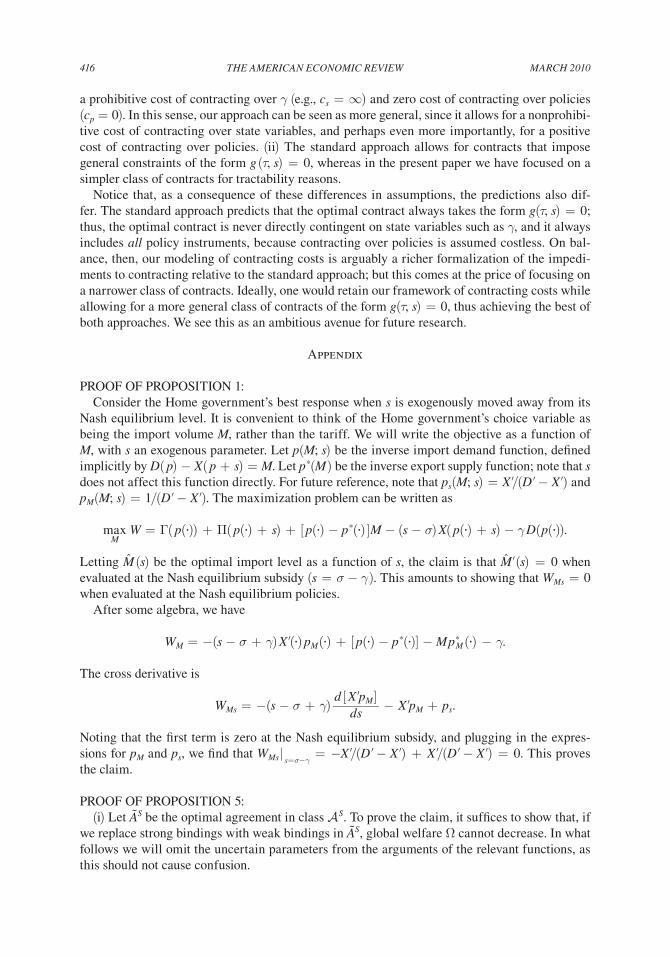
mARcH 2010416 tHE AmERIcAN EcONOmIc REVIEW
a prohibitive cost of contracting over γ (e.g., cs = ∞) and zero cost of contracting over policies (cp = 0). In this sense, our approach can be seen as more general, since it allows for a nonprohibi-tive cost of contracting over state variables, and perhaps even more importantly, for a positive cost of contracting over policies. (ii) The standard approach allows for contracts that impose general constraints of the form g (τ, s) = 0, whereas in the present paper we have focused on a simpler class of contracts for tractability reasons.
Notice that, as a consequence of these differences in assumptions, the predictions also dif-fer. The standard approach predicts that the optimal contract always takes the form g(τ, s) = 0; thus, the optimal contract is never directly contingent on state variables such as γ, and it always includes all policy instruments, because contracting over policies is assumed costless. On bal-ance, then, our modeling of contracting costs is arguably a richer formalization of the impedi-ments to contracting relative to the standard approach; but this comes at the price of focusing on a narrower class of contracts. Ideally, one would retain our framework of contracting costs while allowing for a more general class of contracts of the form g(τ, s) = 0, thus achieving the best of both approaches. We see this as an ambitious avenue for future research.
Appendix
PROOF OF PROPOSITION 1:Consider the Home government’s best response when s is exogenously moved away from its
Nash equilibrium level. It is convenient to think of the Home government’s choice variable as being the import volume m, rather than the tariff. We will write the objective as a function of m, with s an exogenous parameter. Let p(m; s) be the inverse import demand function, defined implicitly by d( p) − X ( p + s) = m. Let p*(m ) be the inverse export supply function; note that s does not affect this function directly. For future reference, note that ps(m; s) = X′/(d′ − X′) and pm(m; s) = 1/(d′ − X′). The maximization problem can be written as
max m
W = Γ( p(·)) + Π( p(·) + s) + [ p(·) − p*(·) ]m − (s − σ) X( p(·) + s) − γ d(p(·)).
Letting ˆ
m (s) be the optimal import level as a function of s, the claim is that ˆ
m ′ (s) = 0 when evaluated at the Nash equilibrium subsidy (s = σ − γ ). This amounts to showing that Wms = 0 when evaluated at the Nash equilibrium policies.
After some algebra, we have
Wm = −(s − σ + γ) X′(·) pm (·) + [ p(·) − p*(·)] − m p*m (·) − γ.
The cross derivative is
Wms = −(s − σ + γ) d [ X′pm ] ______ ds
− X′pm + ps.
Noting that the first term is zero at the Nash equilibrium subsidy, and plugging in the expres-sions for pm and ps, we find that Wms | s=σ−γ = −X′/(d′ − X′) + X′/(d′ − X′) = 0. This proves the claim.
PROOF OF PROPOSITION 5:(i) Let ˜
A s be the optimal agreement in class s. To prove the claim, it suffices to show that, if
we replace strong bindings with weak bindings in ˜
A s, global welfare Ω cannot decrease. In what follows we will omit the uncertain parameters from the arguments of the relevant functions, as this should not cause confusion.

VOL. 100 NO. 1 417HORN Et AL.: ENdOgENOusLy INcOmpLEtE cONtRActs
Agreement ˜
A s can be one of the following types: (a) { t = ̃
t }; (b) { t = ̃
t ; s = ̃ s }; or (c) {Nt ;
τ = ̃ τ ; s = ̃ s }. The bindings ̃
t , ̃ s , ̃ τ , ̃ s may be contingent, but again we omit the state variables
from the notation.Let us start with case (a). Consider replacing { t = ̃
t } with { t ≤ ̃
t }. This can decrease Ω
only if in some state of the world the government chooses t < ̃
t and this implies a lower level of Ω than t = ̃
t . But t will be set below the ceiling only if the noncooperative import tax t N is
lower than the ceiling, in which case the importing country will set t = t N. Let us show that Ω decreases in t for t > t N. Recall that the subsidy is set as s = s R(t ) and note that
d ___ dt
Ω (t, s R(t )) = Wt (t, s R(t )) + d ___ dt
W *(t, s R(t )),
where we have used the envelope theorem to set (d/dt ) W (t, s R(t )) = Wt (t, s R(t )). Clearly Wt < 0 for t > t N. Also, the sign of (d/dt ) W *(t, s R(t )) is the same as the sign of (d/dt ) p*(t, s R(t )), which is negative by assumption. This in turn implies (d/dt ) Ω (t, s R(t )) < 0 for t > t N. We can conclude that switching to a weak binding cannot decrease Ω.
Next, consider case (b), and consider replacing { t = ̃
t ; s = ̃ s } with { t ≤ ̃
t ; s ≤ ̃
s }. For a
given state, there are four relevant possibilities for how the importing country sets ( t, s) under an agreement { t ≤ ̃
t ; s ≤ ̃
s }:
• It chooses ( t = ̃
t , s = ̃ s ): In this case there is, of course, no change in Ω relative to the
strong-binding agreement.
• It chooses ( t = ̃
t , s = s R (t )): Here, it must be that s R (t ) is lower than the ceiling. Let us evaluate Ωs = Ws + Ws
*. Clearly, Ws < 0 for s > s R (t ), and Ws* < 0, hence Ωs < 0 for
s > s R (t ), which in turn implies that switching to weak bindings increases Ω.
• It chooses (t = t R (s ), s = ̃ s ): Here it must be that t R (s ) is below the ceiling. Let us evalu-
ate Ωt = Wt + Wt* . Since Wt < 0 for t > t R (s ), and Wt
* < 0, it follows that Ωt < 0 in this region, which ensures that switching to weak bindings increases Ω.
• It chooses (t = t N, s = s N ): The same result can be shown by combining the arguments we just made for the previous two cases.
Consequently, a switch from { t = ̃
t ; s = ̃ s } to { t ≤ ̃
t ; s ≤ ̃
s } cannot decrease Ω.
Finally, consider case (c). Since the NT-based agreement constrains the wedge q − p* and leaves the wedge p − p* discretionary, it is convenient to redefine variables as follows: p − p* ≡ z and q − p* ≡ v. We can think of z and v as the policy instruments and of the NT-based agreement as imposing a constraint v = ̃ v .
Let us now replace the agreement { Nt ; τ = ̃ τ ; s = ̃ s } with { Nt, τ ≤ ̃ τ , s ≤ ̃ s }. Using the new notation, this is equivalent to replacing the constraint v = ̃ v with the constraint v ≤ ̃ v . In other words, the NT-based agreement with weak bindings effectively places an upper bound on the producer price wedge. We can apply a similar argument as for case (a): it suffices to show that, for any given state, Ω (v, z R (v)) is decreasing in v for v > v N (where v N denotes the unilateral optimum for v and z R (v) the unilateral optimum for z given v). Note that
d ___ dv
Ω (v, z R (v)) = Wv (v, z R (v)) + d ___ dv
W *(v, z R (v)).

mARcH 2010418 tHE AmERIcAN EcONOmIc REVIEW
Clearly, Wv < 0 for v > v N. Next, note that v and z affect W * only through p*, and (d/dv) W *(v, z R(v))has the same sign as (d/dv) p*(v, z R(v)). It is direct to verify that our assumptions imply(d/dv)p*(v, z R(v)) < 0. This in turn implies that switching to weak bindings cannot decrease Ω.
(ii) In the limit, as p*/η* goes to zero, the noncooperative levels of all policy instruments approach their respective efficient levels. Now, recall that the sufficient condition requires that at least one of the bindings in the optimal strong-binding agreement is at least partially rigid. Suppose the optimal strong binding on instrument x is rigid with respect to state variable χ (whose support we denote [ χmin , χmax ] ). It is not hard to show that the optimal strong binding level must be strictly higher than χmin. But, then, it follows immediately that replacing the opti-mal strong binding with a weak binding at the same level will strictly improve the performance of the contract, because there will be realizations of χ such that the noncooperative level of x falls below the binding.
REFERENCES
Bagwell, Kyle, and Robert W. Staiger. 1990. “A Theory of Managed Trade.” American Economic Review, 80(4): 779–95.
Bagwell, Kyle, and Robert W. Staiger. 2001. “Domestic Policies, National Sovereignty, and International Economic Institutions.” Quarterly Journal of Economics, 116(2): 519–62.
Bagwell, Kyle, and Robert W. Staiger. 2002. the Economics of the World trading system. Cambridge, MA: MIT Press.
Bagwell, Kyle, and Robert W. Staiger. 2005. “Enforcement, Private Political Pressure, and the General Agreement on Tariffs and Trade/World Trade Organization Escape Clause.” Journal of Legal studies, 34(2): 471–513.
Bagwell, Kyle, and Robert W. Staiger. 2006. “Will International Rules on Subsidies Disrupt the World Trading System?” American Economic Review, 96(3): 877–95.
Baldwin, Richard E. 1987. “Politically Realistic Objective Functions and Trade Policy: PROFs and Tar-iffs.” Economics Letters, 24(3): 287–90.
Battigalli, Pierpaolo, and Giovanni Maggi. 2002. “Rigidity, Discretion, and the Costs of Writing Con-tracts.” American Economic Review, 92(4): 798–817.
Battigalli, Pierpaolo, and Giovanni Maggi. 2003. “International Agreements on Product Standard: An Incomplete Contracting Theory.” National Bureau of Economic Research Working Paper 9533.
Bhagwati, Jagdish, and V. K. Ramaswami. 1963. “Domestic Distortions, Tariffs and the Theory of Opti-mum Subsidy.” Journal of political Economy, 71(1): 44–50.
Copeland, Brian R. 1990. “Strategic Interaction among Nations: Negotiable and Non-negotiable Trade Barriers.” canadian Journal of Economics, 23(1): 84–108.
Costinot, Arnaud. 2008. “A Comparative Institutional Analysis of Agreements on Product Standards.” Journal of International Economics, 75(1): 197–213.
Ederington, Josh. 2001. “International Coordination of Trade and Domestic Policies.” American Eco-nomic Review, 91(5): 1580–93.
Grossman, Gene M., and Elhanan Helpman. 1994. “Protection for Sale.” American Economic Review, 84(4): 833–50.
Horn, Henrik. 2006. “National Treatment in the GATT.” American Economic Review, 96(1): 394–404.Horn, Henrik, Giovanni Maggi, and Robert W. Staiger. 2008. “Trade Agreements as Endogenously
Incomplete Contracts.” Unpublished.Horn, Henrik, and Petros C. Mavroidis. 2004. “Still Hazy After All These Years: The Interpretation
Of National Treatment In The GATT/WTO Case-Law On Tax Discrimination.” European Journal of International Law, 15(1): 39–69.
Hudec, Robert E. 1990. the gAtt Legal system and World trade diplomacy. 2nd ed. Salem, NH: Butter-worth Legal Publishers.
Johnson, Harry G. 1965. “Optimal Trade Intervention in the Presence of Domestic Distortions.” In trade, growth and the Balance of payments, ed. Richard E. Caves, Harry G. Johnson, and Peter B. Kenen, 3–34. Amsterdam: North-Holland Publishing Company.

VOL. 100 NO. 1 419HORN Et AL.: ENdOgENOusLy INcOmpLEtE cONtRActs
Johnson, Harry G. 1953–54. “Optimum Tariffs and Retaliation.” Review of Economics studies, 21(2):142– 53
Maggi, Giovanni, and Andrés Rodríguez-Clare. 2007. “A Political-Economy Theory of Trade Agree-ments.” American Economic Review, 97(4): 1374–1406.
Maggi, Giovanni, and Robert W. Staiger. 2008. “On the Role and Design of Dispute Settlement Procedures in International Trade Agreements.” National Bureau of Economic Research Working Paper 14067.
Markusen, James R. 1975. “International Externalities and Optimal Tax Structures.” Journal of Interna-tional Economics, 5(1): 15–29.
Schwartz, Warren F., and Alan O. Sykes. 2002. “The Economic Structure of Renegotiation and Dispute Resolution in the World Trade Organization.” Journal of Legal studies, 31(1): 179–204.
Sykes, Alan O. 2005. “Subsidies and Countervailing Measures.” In the World trade Organization: Legal, Economic and political Analysis. Vol. 2, ed. Patrick F. J. Macrory, Arthur E. Appleton, and Michael G. Plummer, 83–107. New York: Springer.


