1 3
DOI 10.1007/s00382-015-2932-3Clim Dyn (2016) 47:1775–1792
The leading modes of decadal SST variability in the Southern Ocean in CMIP5 simulations
Gang Wang1 · Dietmar Dommenget1
Received: 18 May 2015 / Accepted: 29 November 2015 / Published online: 21 December 2015 © Springer-Verlag Berlin Heidelberg 2015
Keywords CMIP5 · Southern Ocean · Climate modes · Decadal variability
1 Introduction
The Southern Ocean (SO), for its large heat and carbon capacity, plays a critical role in the Earth climate system (e.g. Sabine et al. 2004; Séférian et al. 2012). There are evidences that decadal and even longer variability exists in the SO, such as tree rings in Tasmania (Villalba et al. 1997; Cook et al. 2000) and increase of the Antarctic sea ice extent (e.g., Cavalieri and Parkinson 2008; Comiso and Nishio 2008).
However, due mainly to sparse observations, the long-term climate variability of the SO has not been studied extensively especially on the larger scale as its Northern Hemisphere counterpart. For the Sea Surface Tempera-ture (SST) variability, most research focus on the remote response to the El Nino/Southern Oscillation (ENSO) (e.g. Karoly 1989; Kidson and Renwick 2002; Mantua and Hare 2002). The Rossby wave teleconnection patterns in the Southern Hemisphere atmosphere, known as the Pacific South America (PSA) patterns, transport the ENSO cli-mate anomalous signals from the tropics to high southern latitudes (e.g. Mo and Higgins 1998; Renwick 2002; Turner 2004). Another important factor in the SO is the Southern Annular Mode (SAM), which could be defined as the lead-ing EOF pattern of sea level pressure (SLP) between 20° and 70°S and is approximately zonally symmetric, but out of phase between middle and high latitudes (Kidson 1988; Karoly 1990; Thompson and Wallace 2000; Simmonds and King 2004; Jones et al. 2009). The SAM affects the west-erly circumpolar flow, then further influences the circula-tion, temperature distribution, mixed layer depth and heat
Abstract The leading modes of Sea Surface Tempera-ture variability in the Southern Ocean on decadal and even larger time scales are analysed using Coupled Model Inter-comparison Project 5 (CMIP5) model simulations and observations. The analysis is based on Empirical Orthogo-nal Function modes of the CMIP5 model super ensemble. We compare the modes from the CMIP5 super ensemble against several simple null hypotheses, such as isotropic diffusion (red noise) and a Slab Ocean model, to investigate the sources of decadal variability and the physical processes affecting the characteristics of the modes. The results show three main modes in the Southern Ocean: the first and most dominant mode on interannual to decadal time scales is an annular mode with largest amplitudes in the Pacific, which is strongly related to atmospheric forcing by the Southern Annular Mode and El Nino Southern Oscillation. The sec-ond mode is an almost basin wide monopole pattern, which has pronounced multi-decadal and longer time scales vari-ability. It is firstly inducted by the Wave-3 patterns in the atmosphere and further developed via ocean dynamics. The third mode is a dipole pattern in the southern Pacific that has a pronounced peak in the power spectrum at multi-decadal time scales. All three leading modes found in the CMIP5 super model have distinct patterns and time scale behaviour that can not be explained by simple stochastic null hypothesis, thus all three leading modes are ocean–atmosphere coupled modes and are likely to be substan-tially influenced or driven by ocean dynamical processes.
* Gang Wang [email protected]
1 School of Earth, Atmosphere and Environment, Monash University, Clayton, VIC 3800, Australia

1776 G. Wang, D. Dommenget
1 3
capacity in the ocean via the Ekman pumping effect (e.g. Boer et al. 2001; Cai and Watterson 2002; Fyfe 2003). Recent studies suggest that a quasi-decadal variability exists in the SAM (Yuan and Li 2008; Yuan and Yonekura 2011).
Within the deeper subsurface SO, the intrinsic variabil-ity is closely related to the Antarctic Circumpolar Current (ACC). The baroclinic instability originates within the thermocline of the ACC (O’Kane et al. 2013; Monsele-san et al. 2015), and further results into positive feedbacks between meso-scale eddies and the ACC mean flow (Hogg and Blundell 2006). On even longer-term variability the Southern Ocean centennial variability is possibly caused by deep ocean overturning circulation changes, as discussed in model based studies (e.g. Latif et al. 2013).
Further, a number of modes in the atmosphere–ocean system have been identified in the Southern Hemisphere, such as the Trans-Polar Index (TPI, Jones et al. 1999), Ant-arctic Circumpolar Wave (ACW, e.g. White and Peterson 1996; White et al. 2004; White and Simmonds 2006) and South Pacific subtropical Dipole (Morioka et al. 2013). They might also exhibit decadal variations, which are still unclear (e.g., Simmonds 2003; Yuan and Yonekura 2011).
The length of observational records and limitations of mod-els restrict our understanding of the long-term variability in the Southern Ocean. Besides, most previous studies focus on the modes from the atmosphere rather than from the ocean, mainly because of the relative abundance of the atmospheric data. However, as the significant heat content of the SO, the ocean itself should have more influence on the decadal and even longer variations. In this study presented here we will base our SST variability analyses within SO on the empirical orthogonal function (EOF) modes in the model simulations and observations, and get the basic SST modes in SO on the low frequency as well as their features and influencing factors. We will also compare the leading modes of variability against simple null hypotheses such as isotropic diffusion (red noise) and atmospheric forcings only (Slab Ocean simulation), to test the factors that influence the generation and proposition of the modes (see Dommenget 2007; Wang et al. 2015).
The paper is organized as follows: firstly, Sect. 2 pre-sents the data used. Section 3 evaluates the consistency of CMIP5 simulations. The main results of this study are shown in Sect. 4. Here the leading modes in the Southern Ocean and their features are presented and analysis of the sources of the modes and the factors affecting their main characteristics are presented. Finally a summary and dis-cussion are provided in Sect. 5.
2 Data, model simulations and methods
The observed global monthly mean SSTs are taken from the NOAA Optimum Interpolation Sea Surface Temperature
(OISST) V2 from 1982 to 2004, which are based on in situ and satellite observations (referred as “observations” below, Reynolds et al. 2002). Hadley Centre Sea Ice and SST data set (HadISST, Rayner et al. 2003) was chosen as an auxiliary.
Our analysis focuses on the long-term internal natural variability, therefore the scenario of CMIP5 “pre-industrial control” (PiControl) is used for the following study for its relatively long output without anthropogenic forcing influ-ence. 10 CMIP5 models (Table 1) are selected from the CMIP5 datasets (Taylor et al. 2012), as they represent all the models having at least 500 years continuous simulation and all the variable outputs needed for the analysis in this paper. We take 500 years from each model and concatenate the SST anomalies (computed for each model individually) to generate a CMIP5 super model with 5000 years of data to provide a synthesis. This kind of super model has been shown to be more similar to the observed modes than indi-vidual models (Bayr and Dommenget 2014; Wang et al. 2015). We will further verify the super model performance in Sect. 3.
We also use a 500 year simulation of an atmospheric GCM coupled to a simple Slab Ocean to compare against the CMIP5 models. This model is comprised of the UK Meteorological Office Unified Model general circulation model with HadGEM2 atmospheric physics, a Slab Ocean model with a 50 m-layer thickness and prescribed sea ice monthly climatology of 1950–2010.
The slab ocean cannot reproduce realistic mean SST without calibration, as it does not include ocean circulation to maintain the observed surface energy balance. Therefore, a flux correction scheme is used to force the model SST
Table 1 List of CMIP5 models
Number Originating group(s) Country Model
1 CSIRO and BOM Australia ACCESS1.0
2 CSIRO and BOM Australia ACCESS1.3
3 National Center for Atmospheric Research
USA CCSM4
4 Canadian Centre for Climate Modelling and Analysis
Canada CanESM2
5 Geophysical Fluid Dynamics Laboratory
USA GFDL-CM3
6 Geophysical Fluid Dynamics Laboratory
USA GFDL-ESM2G
7 Hadley Centre for Climate Prediction and Research/ Met Office
UK HadGEM2-ES
8 Institut Pierre Simon Laplace France IPSL-CM5A-LR
9 Meteorological Research Institute
Japan MRI-CGCM3
10 Beijing Climate Center China bcc-csm1-1
1777The leading modes of decadal SST variability in the Southern Ocean in CMIP5 simulations
1 3
to closely follow the Hadley Centre Sea Ice and SST data set (HadISST) SST climatology (for more details see Wang et al. 2015). The flux corrections are a function of location and calendar month, but are identical in every year and are thus not state dependent. They are constant fluxes that lead to the correct seasonal mean SST, but do not directly force any SST anomalies. The application of a flux correction to the ocean surface energy balance is an alternative way of introducing a parameterization of the ocean circulation, however, the circulation in the slab ocean model is effec-tively fixed and does not change in response to atmospheric forcings.
All data sets (models and observations) were interpo-lated to a common 2.5° latitude × longitude grid and lin-early detrended to remove the global warming signal and/or climate drift prior to the analysis.
The concept of the data set SST mode comparison is based on Dommenget (2007) and Bayr and Dommenget (2014), and has been applied in a similar way to the SO SST modes in Wang et al. (2015). It is briefly summarized as follows: Assume there are two data sets A and B. cij is the correlation coefficient describing the spatial similarity between �EA
i , the ith EOF-pattern of A, and �EBi , the jth EOF-
pattern of B. The total variance of B that can be explained by �EA
i , namely projected explained variance (PEV) peiA→B,
is estimated by the accumulation of all eigenvalues of B:
where ejB is the explained variance of the correspond-
ing EOF-pattern. The overall mismatch between A and B is quantified by a normalized root-mean-square error (RMSEEOF)
where A is the reference data. RMSEEOF ranges from 0 to 1 and estimates the inconsistency between two data sets. The larger the value is, the larger are the differences in spatial structure in variability.
Apart from the EOF projection method above, we also use the distinct EOFs (DEOFs) to estimate the pat-terns that describe the largest differences in explained variance between two data sets A and B (Dommenget 2007), which are found by pairwise rotation of the EOF-modes to maximize the leading ei
A values relative to the peA→B
i iteratively (Dommenget 2007; Bayr and Dom-menget 2014). Each DEOF mode has two explained variance values. One is the explained variance in dataset A, devi
A→B(A), and the other the explained variance in B, devi
A→B(B). The DEOFs patterns are ordered by the
(1)peA→Bi =
N∑
j=1
c2ijeBj
(2)RMSEEOF(A,B) =
√
√
√
√
∑Ni=1
(
peA→Bi − eAi
)2
∑Ni=1
(
eAi
)2
difference between deviA→B(A) and devi
A→B(B). There-fore, the first DEOF mode, DEOF1
A→B, would represent the pattern that explains more variance in A than in B, and this difference should be the largest among all DEOF patterns. Thus, DEOFs is a simple way to illustrate the largest differences between two datasets demonstrating significant differences in terms of spatial patterns, how-ever, they may have some limitations in the interpreta-tion similar to those of EOF patterns (for more details see Dommenget 2007).
3 Model evaluation
Wang et al. (2015) showed, in an evaluation of the SST modes for CMIP5 historical runs in the Southern Ocean, that the all models differ significantly with the HadISST modes with the uncertainties in the order of 40–60 % of the eigenvalues. The study also illustrated larger inconsist-ency of the model with each other via pairwise model com-parison. However, the super model ensemble showed better agreement with the references, suggesting that it has spatial modes similar to the observed and should be more suita-ble for further data analysis. To verify the reliability of the models in the study here, especially the super ensemble, we will do a similar evaluation, but for the CMIP5 PiControl simulations against the OISST data.
Figure 1 shows the leading modes of Southern Ocean monthly mean SST anomalies (south of 30°S) to get a first impression of how similar model simulations and observa-tions are. Each EOF pattern is multiplied by the root of its own eigenvalue for consistency so that the amplitude of all patterns is in the unit of Kelvin. There are clear similarities between the observed and the CMIP5 super ensemble. They both have the annular mode as the EOF-1, with the similar structure: maximum anomaly amplitude in the South Pacific and the out-of-phase zonal anomalies around 30°–45°S (Fig. 1a, d). The CMIP5 super ensemble also has a similar wave train like EOF-3 as observed (Fig. 1c, f). However, the EOF-2 in CMIP5 is more like a wave-3 pattern along 60°S with two weak troughs (Fig. 1e) while differently the observed EOF-2 composes of 4 waves (Fig. 1b).
The Slab Ocean results (Fig. 1g–i) illustrate more dif-ferences with much larger eigenvalues compared to obser-vations and CMIP5 data. Its EOF-1 (Fig. 1g) shows simi-lar wave-3 structure as CMIP5 EOF-2, but the two weak troughs get much stronger in the Slab Ocean simulation south to Africa/Australia. Another wave-3 pattern also exists within the Slab Ocean EOF-2 (Fig. 1h) and its anom-aly centres in the Pacific are in the same location as the annular mode (EOF-1) in CMIP5 and the observed. Last, Slab Ocean has a similar wave-like EOF-3 as its counter-parts but with lower latitude centres.

1778 G. Wang, D. Dommenget
1 3
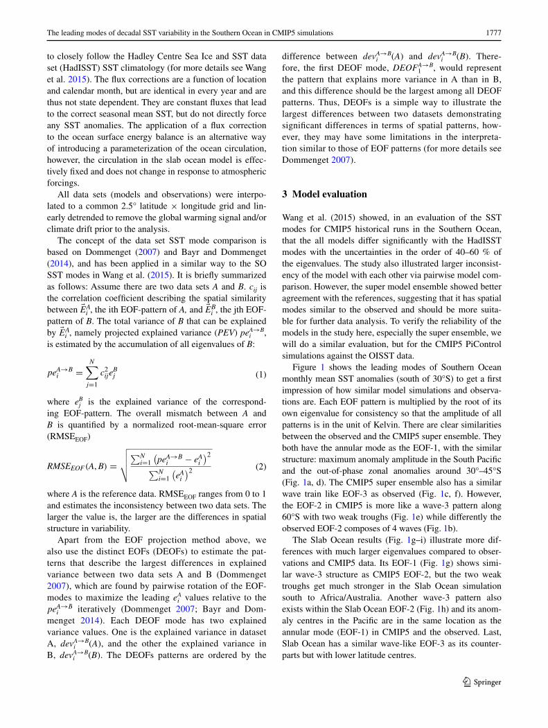
To quantify the differences among data sets, Fig. 2 presents the RMSEEOF with OISST as reference on the x-axis and all models as references on the y-axis. The values on the y-axis are the mean RMSEEOF of
all pairwise comparison with all individual models as references.
OISST and HadISST for the same period (1982–2014) agree well with each other, since the two observational data
EOF1 EOF2 EOF3
Observed
(a) 11.6% (b) 7.2% (c) 7.0%
CMIP5
(d) 13.5% (e) 6.8% (f) 5.8%
Slab Ocean
(g) 16.4% (h) 12.6% (i) 8.2%
150 oW
120 oW
90o W
60o W
30o W
0o
30 oE
60 oE90
oE
120
o E
150o E
180oW
75oS
60oS
45oS150 oW
120 oW
90o W
60o W
30o W
0o
30 oE
60 oE90
oE
120
o E
150o E
180oW
75oS
60oS
45oS
150 oW
120 oW
90o W
60o W
30o W
0o
30 oE
60 oE90
oE
120
o E
150o E
180oW
75oS
60oS
45oS
150 oW
120 oW
90o W
60o W
30o W
0o
30 oE
60 oE90
oE
120
o E
150o E
180oW
75oS
60oS
45oS150 oW
120 oW
90o W
60o W
30o W
0o
30 oE
60 oE90
oE
120
o E150
o E
180oW
75oS
60oS
45oS
150 oW
120 oW
90o W
60o W
30o W
0o
30 oE
60 oE90
oE
120
o E
150o E
180oW
75oS
60oS
45oS
150 oW
120 oW
90o W
60o W
30o W
0o
30 oE
60 oE90
oE
120
o E
150o E
180oW
75oS
60oS
45oS150 oW
120 oW
90o W
60o W
30o W
0o
30 oE
60 oE90
oE
120
o E
150o E
180oW
75oS
60oS
45oS
150 oW
120 oW
90o W
60o W
30o W
0o
30 oE
60 oE90
oE
120
o E
150o E
180oW
75oS
60oS
45oS
Fig. 1 First three leading EOF patterns of detrended monthly SSTA in the Southern Ocean for a–c Observation (OISST); d–f CMIP5 super model; g–i slab ocean experiment. The values in the headings of each panel are the explained variances of each EOF-mode
1779The leading modes of decadal SST variability in the Southern Ocean in CMIP5 simulations
1 3
sets contain the same observations. However, the HadISST data for the much longer period (1901–2014) disagrees with the OISST data substantially. This is most likely due to the sparse observations prior to the 1980s. The relative errors of most models are ranging from 20 to 45 % of the eigenvalues, which are substantial and similar as the dif-ference between Slab Ocean and the observed (29 %). The CMIP5 super model performs better (28 %) than most models and has by construction much longer statistics than any individual model, which suggests that the super model is the best data set for the following analysis.
For the model pairwise comparison, most models are in the range of 20–50 %, while the observed has larger bias of 50–65 %. This indicates that models have strong differences and disagreements in the spatial structures between each other. Again the super model is better than most individual models with an error of 26 %, implying the model ensemble should be a good substitution of an individual model.
The slab ocean shows substantial difference relative to the fully-coupled models (60 % error), which suggest that the dynamics of the CMIP5 models are significantly differ-ent than in the slab ocean model. Additionally, we introduce two categories of isotropic diffusions representing homoge-neous spatial red noise processes (refer as H0uniform) and spatial red noise with known standard spatial deviation pat-tern (refer as H0STDV) (see Dommenget 2007; Wang et al. 2015 for details). Both these simple stochastic models are farther away from the observations than any individual model, suggesting that the SST modes in the Southern Ocean are indeed related to more complex dynamics than assumed in the simple null hypotheses.
4 Leading modes in the Southern Ocean
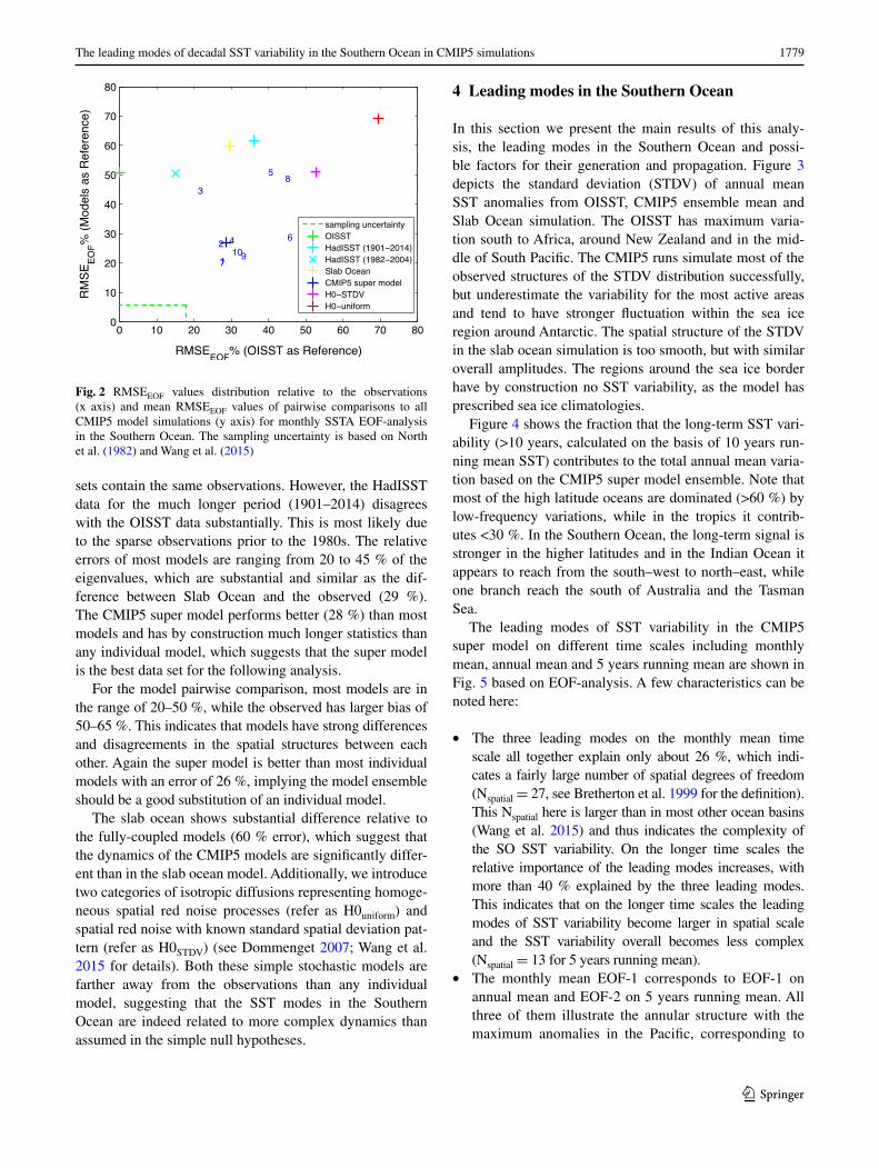
In this section we present the main results of this analy-sis, the leading modes in the Southern Ocean and possi-ble factors for their generation and propagation. Figure 3 depicts the standard deviation (STDV) of annual mean SST anomalies from OISST, CMIP5 ensemble mean and Slab Ocean simulation. The OISST has maximum varia-tion south to Africa, around New Zealand and in the mid-dle of South Pacific. The CMIP5 runs simulate most of the observed structures of the STDV distribution successfully, but underestimate the variability for the most active areas and tend to have stronger fluctuation within the sea ice region around Antarctic. The spatial structure of the STDV in the slab ocean simulation is too smooth, but with similar overall amplitudes. The regions around the sea ice border have by construction no SST variability, as the model has prescribed sea ice climatologies.
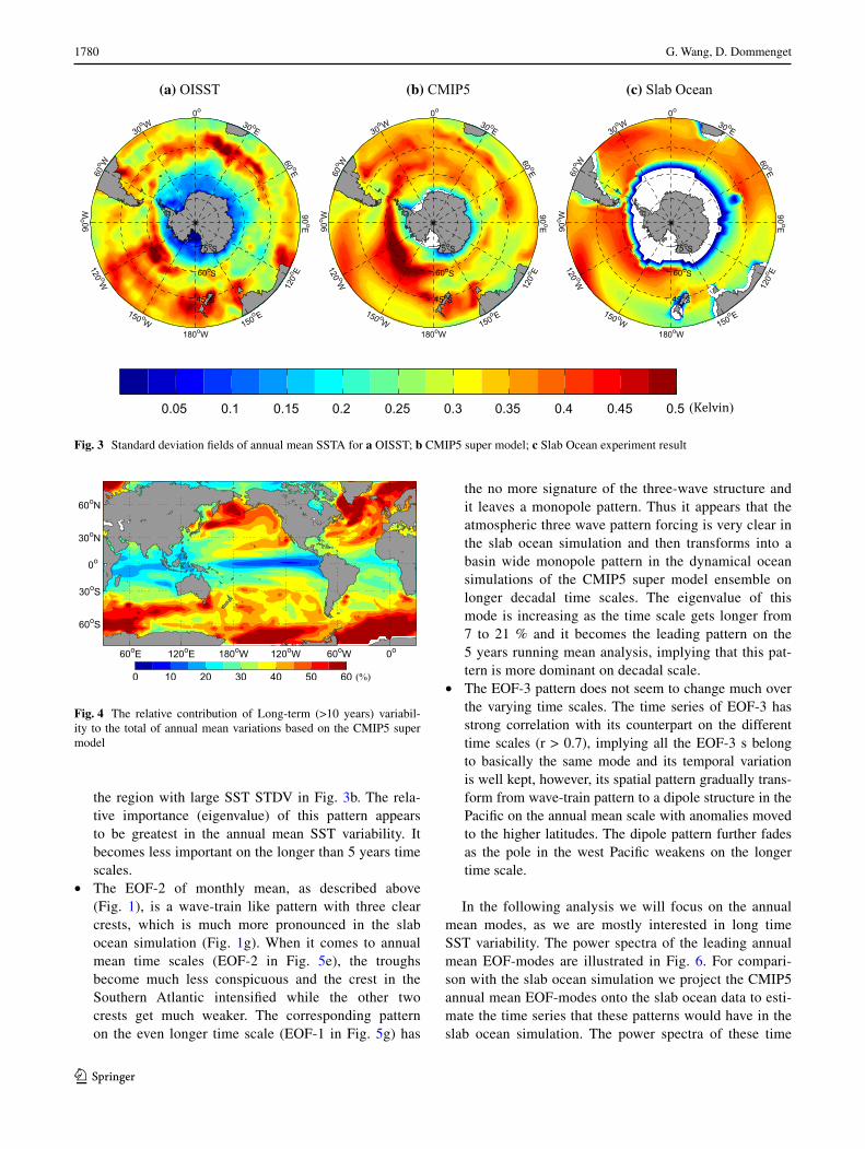
Figure 4 shows the fraction that the long-term SST vari-ability (>10 years, calculated on the basis of 10 years run-ning mean SST) contributes to the total annual mean varia-tion based on the CMIP5 super model ensemble. Note that most of the high latitude oceans are dominated (>60 %) by low-frequency variations, while in the tropics it contrib-utes <30 %. In the Southern Ocean, the long-term signal is stronger in the higher latitudes and in the Indian Ocean it appears to reach from the south–west to north–east, while one branch reach the south of Australia and the Tasman Sea.
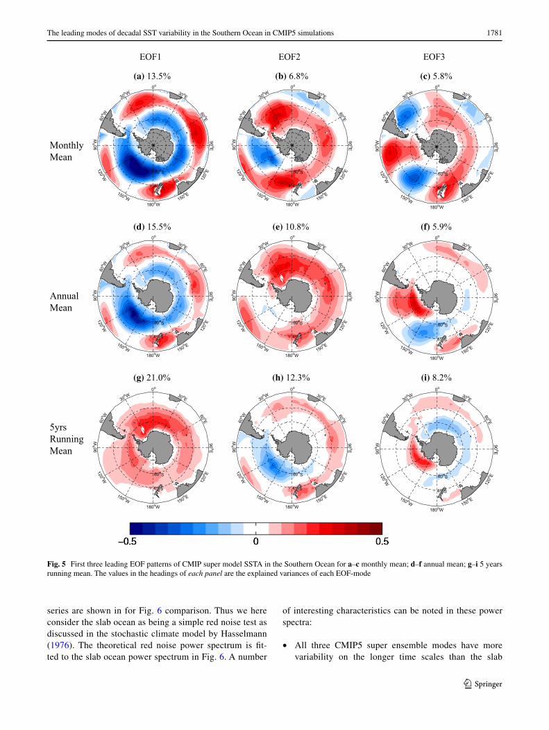
The leading modes of SST variability in the CMIP5 super model on different time scales including monthly mean, annual mean and 5 years running mean are shown in Fig. 5 based on EOF-analysis. A few characteristics can be noted here:
• The three leading modes on the monthly mean time scale all together explain only about 26 %, which indi-cates a fairly large number of spatial degrees of freedom (Nspatial = 27, see Bretherton et al. 1999 for the definition). This Nspatial here is larger than in most other ocean basins (Wang et al. 2015) and thus indicates the complexity of the SO SST variability. On the longer time scales the relative importance of the leading modes increases, with more than 40 % explained by the three leading modes. This indicates that on the longer time scales the leading modes of SST variability become larger in spatial scale and the SST variability overall becomes less complex (Nspatial = 13 for 5 years running mean).
• The monthly mean EOF-1 corresponds to EOF-1 on annual mean and EOF-2 on 5 years running mean. All three of them illustrate the annular structure with the maximum anomalies in the Pacific, corresponding to
Fig. 2 RMSEEOF values distribution relative to the observations (x axis) and mean RMSEEOF values of pairwise comparisons to all CMIP5 model simulations (y axis) for monthly SSTA EOF-analysis in the Southern Ocean. The sampling uncertainty is based on North et al. (1982) and Wang et al. (2015)
1780 G. Wang, D. Dommenget
1 3
the region with large SST STDV in Fig. 3b. The rela-tive importance (eigenvalue) of this pattern appears to be greatest in the annual mean SST variability. It becomes less important on the longer than 5 years time scales.
• The EOF-2 of monthly mean, as described above (Fig. 1), is a wave-train like pattern with three clear crests, which is much more pronounced in the slab ocean simulation (Fig. 1g). When it comes to annual mean time scales (EOF-2 in Fig. 5e), the troughs become much less conspicuous and the crest in the Southern Atlantic intensified while the other two crests get much weaker. The corresponding pattern on the even longer time scale (EOF-1 in Fig. 5g) has
the no more signature of the three-wave structure and it leaves a monopole pattern. Thus it appears that the atmospheric three wave pattern forcing is very clear in the slab ocean simulation and then transforms into a basin wide monopole pattern in the dynamical ocean simulations of the CMIP5 super model ensemble on longer decadal time scales. The eigenvalue of this mode is increasing as the time scale gets longer from 7 to 21 % and it becomes the leading pattern on the 5 years running mean analysis, implying that this pat-tern is more dominant on decadal scale.
• The EOF-3 pattern does not seem to change much over the varying time scales. The time series of EOF-3 has strong correlation with its counterpart on the different time scales (r > 0.7), implying all the EOF-3 s belong to basically the same mode and its temporal variation is well kept, however, its spatial pattern gradually trans-form from wave-train pattern to a dipole structure in the Pacific on the annual mean scale with anomalies moved to the higher latitudes. The dipole pattern further fades as the pole in the west Pacific weakens on the longer time scale.
In the following analysis we will focus on the annual mean modes, as we are mostly interested in long time SST variability. The power spectra of the leading annual mean EOF-modes are illustrated in Fig. 6. For compari-son with the slab ocean simulation we project the CMIP5 annual mean EOF-modes onto the slab ocean data to esti-mate the time series that these patterns would have in the slab ocean simulation. The power spectra of these time
(a) OISST (b) CMIP5
150 oW
120 oW
90o W
60o W
30o W
0o
30 oE
60 oE90
oE
120
o E
150o E
180oW
75oS
60oS
45oS150 oW
120 oW
90o W
60o W
30o W
0o
30 oE
60 oE90
oE
120
o E
150o E
180oW
75oS
60oS
45oS150 oW
120 oW
90o W
60o W
30o W
0o
30 oE
60 oE90
oE
120
o E
150o E
180oW
75oS
60oS
45oS
0.05 0.1 0.15 0.2 0.25 0.3 0.35 0.4 0.45 0.5
(c) Slab Ocean
Fig. 3 Standard deviation fields of annual mean SSTA for a OISST; b CMIP5 super model; c Slab Ocean experiment result
(%)
60oE 120oE 180oW 120oW 60oW 0o
oS
oS
o
oN
60
30
0
30
60oN
0 10 20 30 40 50 60
Fig. 4 The relative contribution of Long-term (>10 years) variabil-ity to the total of annual mean variations based on the CMIP5 super model
1781The leading modes of decadal SST variability in the Southern Ocean in CMIP5 simulations
1 3
series are shown in for Fig. 6 comparison. Thus we here consider the slab ocean as being a simple red noise test as discussed in the stochastic climate model by Hasselmann (1976). The theoretical red noise power spectrum is fit-ted to the slab ocean power spectrum in Fig. 6. A number
of interesting characteristics can be noted in these power spectra:
• All three CMIP5 super ensemble modes have more variability on the longer time scales than the slab
EOF1 EOF2 EOF3
MonthlyMean
(a) 13.5% (b) 6.8% (c) 5.8%
AnnualMean
(d) 15.5% (e) 10.8%
5yrsRunningMean
(g) 21.0% (h) 12.3% (i) 8.2%
150 oW
120 oW
90o W
60o W
30o W
0o
30 oE
60 oE90
oE
120
o E150
o E
180oW
75oS
60oS
45oS150 oW
120 oW
90o W
60o W
30o W
0o
30 oE
60 oE90
oE
120
o E
150o E
180oW
75oS
60oS
45oS
150 oW
120 oW
90o W
60o W
30o W
0o
30 oE
60 oE90
oE
120
o E
150o E
180oW
75oS
60oS
45oS
150 oW
120 oW
90o W
60o W
30o W
0o
30 oE
60 oE90
oE
120
o E
150o E
180oW
75oS
60oS
45oS150 oW
120 oW
90o W
60o W
30o W
0o
30 oE
60 oE90
oE
120
o E150
o E
180oW
75oS
60oS
45oS
150 oW
120 oW
90o W
60o W
30o W
0o
30 oE
60 oE90
oE
120
o E
150o E
180oW
75oS
60oS
45oS
150 oW
120 oW
90o W
60o W
30o W
0o
30 oE
60 oE90
oE
120
o E
150o E
180oW
75oS
60oS
45oS150 oW
120 oW
90o W
60o W
30o W
0o
30 oE
60 oE90
oE
120
o E
150o E
180oW
75oS
60oS
45oS
150 oW
120 oW
90o W
60o W
30o W
0o
30 oE
60 oE90
oE
120
o E
150o E
180oW
75oS
60oS
45oS
(f) 5.9%
Fig. 5 First three leading EOF patterns of CMIP super model SSTA in the Southern Ocean for a–c monthly mean; d–f annual mean; g–i 5 years running mean. The values in the headings of each panel are the explained variances of each EOF-mode

1782 G. Wang, D. Dommenget
1 3
(a) EOF-1 (b) EOF-2 (c) EOF-3
Fig. 6 Spectrum of the time series of the three leading EOF-modes of the CMIP super model annual mean SSTA (as in Fig. 5d–f). The power spectrum of the time series resulting from the projection of these patterns onto the slab ocean simulation SST variability are
shown for comparison. The black line is a red noise fit to the slab ocean time series and the red lines mark the 95 % confidence interval relative to the red noise fit of the slab ocean simulation
EOF1 EOF2 EOF3
SlabOcean
(a) 18.6% (b) 13.2% (c) 9.7%
H0-STDV
(d) 13.9% (e) 10.5% (f) 8.3%
150 oW
120 oW
90o W
60o W
30o W
0o
30 oE
60 oE90
oE
120
o E
150o E
180oW
75oS
60oS
45oS150 oW
120 oW
90o W
60o W
30o W
0o
30 oE
60 oE90
oE
120
o E
150o E
180oW
75oS
60oS
45oS150 oW
120 oW
90o W
60o W
30o W
0o
30 oE
60 oE90
oE
120
o E
150o E
180oW
75oS
60oS
45oS
150 oW
120 oW
90o W
60o W
30o W
0o
30 oE
60 oE90
oE
120
o E
150o E
180oW
75oS
60oS
45oS150 oW
120 oW
90o W
60o W
30o W
0o
30 oE
60 oE90
oE
120
o E
150o E
180oW
75oS
60oS
45oS150 oW
120 oW
90o W
60o W
30o W
0o
30 oE
60 oE90
oE
120
o E
150o E
180oW
75oS
60oS
45oS
Fig. 7 First three leading EOF patterns of detrended annual mean SSTA in the Southern Ocean for a–c slab ocean; d–f H0-STDV null hypoth-esis. The values in the headings of each panel are the explained variances of each EOF-mode
1783The leading modes of decadal SST variability in the Southern Ocean in CMIP5 simulations
1 3
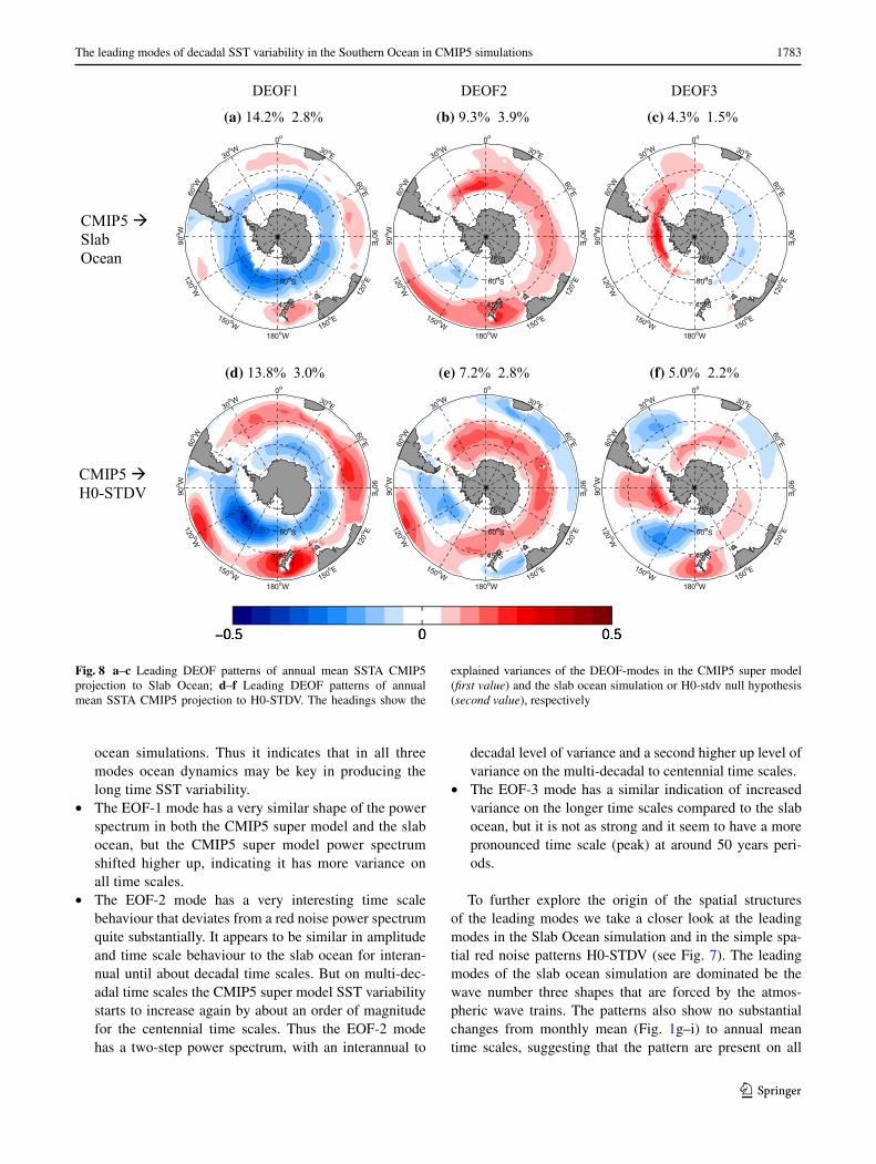
ocean simulations. Thus it indicates that in all three modes ocean dynamics may be key in producing the long time SST variability.
• The EOF-1 mode has a very similar shape of the power spectrum in both the CMIP5 super model and the slab ocean, but the CMIP5 super model power spectrum shifted higher up, indicating it has more variance on all time scales.
• The EOF-2 mode has a very interesting time scale behaviour that deviates from a red noise power spectrum quite substantially. It appears to be similar in amplitude and time scale behaviour to the slab ocean for interan-nual until about decadal time scales. But on multi-dec-adal time scales the CMIP5 super model SST variability starts to increase again by about an order of magnitude for the centennial time scales. Thus the EOF-2 mode has a two-step power spectrum, with an interannual to
decadal level of variance and a second higher up level of variance on the multi-decadal to centennial time scales.
• The EOF-3 mode has a similar indication of increased variance on the longer time scales compared to the slab ocean, but it is not as strong and it seem to have a more pronounced time scale (peak) at around 50 years peri-ods.
To further explore the origin of the spatial structures of the leading modes we take a closer look at the leading modes in the Slab Ocean simulation and in the simple spa-tial red noise patterns H0-STDV (see Fig. 7). The leading modes of the slab ocean simulation are dominated be the wave number three shapes that are forced by the atmos-pheric wave trains. The patterns also show no substantial changes from monthly mean (Fig. 1g–i) to annual mean time scales, suggesting that the pattern are present on all
DEOF1 DEOF2 DEOF3
(a) 14.2% 2.8% (b) 9.3% 3.9% (c) 4.3% 1.5%
(d) 13.8% 3.0% (e) 7.2% 2.8% (f) 5.0% 2.2%
150 oW
120 oW
90o W
60o W
30o W
0o
30 oE
60 oE90
oE
120
o E
150o E
180oW
75oS
60oS
45oS150 oW
120 oW
90o W
60o W
30o W
0o
30 oE
60 oE90
oE
120
o E
150o E
180oW
75oS
60oS
45oS150 oW
120 oW
90o W
60o W
30o W
0o
30 oE
60 oE90
oE
120
o E
150o E
180oW
75oS
60oS
45oS
150 oW
120 oW
90o W
60o W
30o W
0o
30 oE
60 oE90
oE
120
o E
150o E
180oW
75oS
60oS
45oS150 oW
120 oW
90o W
60o W
30o W
0o
30 oE
60 oE90
oE
120
o E150
o E
180oW
75oS
60oS
45oS150 oW
120 oW
90o W
60o W
30o W
0o
30 oE
60 oE90
oE
120
o E
150o E
180oW
75oS
60oS
45oS
Fig. 8 a–c Leading DEOF patterns of annual mean SSTA CMIP5 projection to Slab Ocean; d–f Leading DEOF patterns of annual mean SSTA CMIP5 projection to H0-STDV. The headings show the
explained variances of the DEOF-modes in the CMIP5 super model (first value) and the slab ocean simulation or H0-stdv null hypothesis (second value), respectively
1784 G. Wang, D. Dommenget
1 3
time scales. The simple spatial red noise H0-STDV EOF-modes are a hierarchy of multi-poles (Fig. 7d–f), starting with a monopole (largest scale), followed by dipoles with increasing complexity (see Dommenget 2007 for a more detailed discussion). These multi-pole modes are centered on the regions of large SST STDV (see Fig. 3b).
The modes of the Slab Ocean simulation and H0-STDV stochastic null hypothesis are clearly different to CMIP5 super model ones. The DEOF modes shown in Fig. 8 fur-ther quantify these differences. The DEOF modes repre-sent the modes that in the comparison between the CMIP5 super model and the Slab Ocean simulation or H0-STDV stochastic null hypothesis are most dominant in the CMIP5 super model (see methods section for details on the DEOF-modes).
Most of the leading DEOF modes duplicate the leading CMIP5 modes in Fig. 5d–f, suggesting that the Slab Ocean and red noise H0-STDV process do not produce these lead-ing modes with enough variance. This is also consistent with the comparison of the power spectra in Fig. 6, where we found that the slab ocean power spectrum of EOF-1 was much weaker than in the CMIP5 super model. One exception is the DEOF-3 for the Slab Ocean (Fig. 8c). This DEOF mode is not similar to the CMIP5 EOF-3 and is more concentrated around the Antarctica.
In summary of this first part of this analysis we can say that we have three leading modes of SST variability on the interannual and long time scales, and all three are fairly different in either their patterns or in their amount of vari-ance from what you would expect from a simple red noise integration of atmospheric forcings. Thus all three modes are likely to involve ocean dynamics to create the pattern or at least the amount of variance. In the following we want to discuss the characteristics of these modes a bit more in detail. However, it will be beyond the scope of this work to fully explain the physical mechanisms of all three leading modes.
4.1 Mode 1: The annular mode
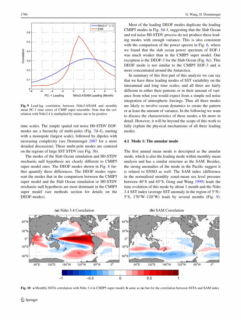
The first annual mean mode is descripted as the annular mode, which is also the leading mode within monthly mean analysis and has a similar structure as the SAM. Besides, the strong anomalies of the mode in the Pacific suggest it is related to ENSO as well. The SAM index (difference in the normalized monthly zonal-mean sea level pressure between 40°S and 65°S, Gong and Wang 1999) leads the time evolution of this mode by about 1 month and the Niño 3.4 SST index (average SST anomaly in the region of 5°N–5°S, 170°W–120°W) leads by several months (Fig. 9).
Fig. 9 Lead-lag correlation between Niño3.4/SAM and monthly mean PC-1 time series of CMIP super ensemble. Note that the cor-relation with Niño3.4 is multiplied by minus one to be positive
(a) Niño 3.4 Correlation (b) SAM Correlation
60oE 120oE 180oW 120oW 60oW 0o
60oS
30oS
0o
30oN
60oN
60oE 120oE 180oW 120oW 60oW 0o
60oS
30oS
0o
30oN
60oN
Fig. 10 a Monthly SSTA correlation with Niño 3.4 in CMIP5 super model; b same as (a) but for the correlation between SSTA and SAM index
1785The leading modes of decadal SST variability in the Southern Ocean in CMIP5 simulations
1 3
Thus we have two important atmospheric teleconnections that drive this mode. The global monthly mean SSTA cor-relation with Niño 3.4 and SAM indices are also shown in Fig. 10. Obviously the correlation focuses within the South Pacific domain in the Southern Ocean when correlated with ENSO, while the SAM correlation is extended to the entire ocean.
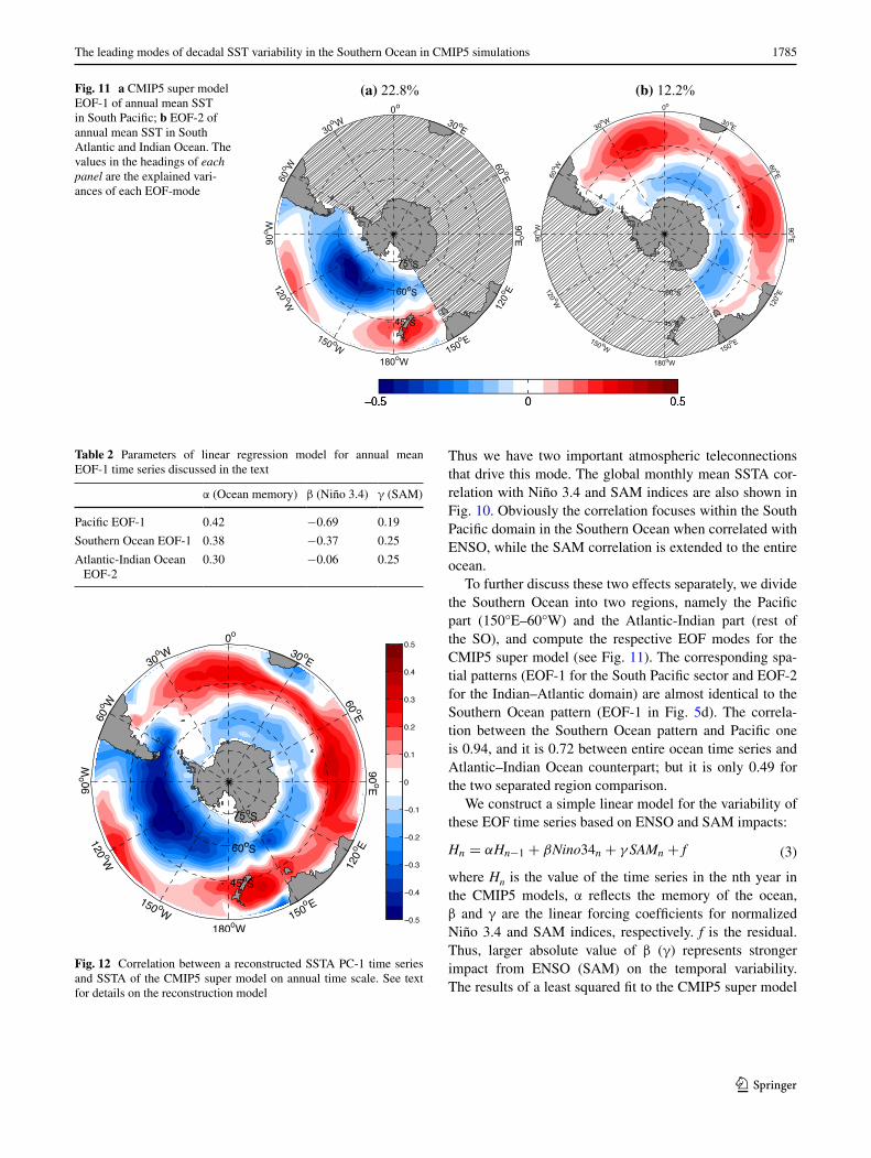
To further discuss these two effects separately, we divide the Southern Ocean into two regions, namely the Pacific part (150°E–60°W) and the Atlantic-Indian part (rest of the SO), and compute the respective EOF modes for the CMIP5 super model (see Fig. 11). The corresponding spa-tial patterns (EOF-1 for the South Pacific sector and EOF-2 for the Indian–Atlantic domain) are almost identical to the Southern Ocean pattern (EOF-1 in Fig. 5d). The correla-tion between the Southern Ocean pattern and Pacific one is 0.94, and it is 0.72 between entire ocean time series and Atlantic–Indian Ocean counterpart; but it is only 0.49 for the two separated region comparison.
We construct a simple linear model for the variability of these EOF time series based on ENSO and SAM impacts:
where Hn is the value of the time series in the nth year in the CMIP5 models, α reflects the memory of the ocean, β and γ are the linear forcing coefficients for normalized Niño 3.4 and SAM indices, respectively. f is the residual. Thus, larger absolute value of β (γ) represents stronger impact from ENSO (SAM) on the temporal variability. The results of a least squared fit to the CMIP5 super model
(3)Hn = αHn−1 + βNino34n + γ SAMn + f
Fig. 11 a CMIP5 super model EOF-1 of annual mean SST in South Pacific; b EOF-2 of annual mean SST in South Atlantic and Indian Ocean. The values in the headings of each panel are the explained vari-ances of each EOF-mode
(a) 22.8% (b) 12.2%
150 oW
120 oW
90o W
60o W
30o W
0o
30 oE
60 oE90
oE
120
o E
150o E
180oW
75oS
60oS
45oS
150 oW
120 oW
90o W
60o W
30o W
0o
30 oE
60 oE
90oE
120
o E
150o E
180oW
75oS
60oS
45oS
Table 2 Parameters of linear regression model for annual mean EOF-1 time series discussed in the text
α (Ocean memory) β (Niño 3.4) γ (SAM)
Pacific EOF-1 0.42 −0.69 0.19
Southern Ocean EOF-1 0.38 −0.37 0.25
Atlantic-Indian Ocean EOF-2
0.30 −0.06 0.25
Fig. 12 Correlation between a reconstructed SSTA PC-1 time series and SSTA of the CMIP5 super model on annual time scale. See text for details on the reconstruction model
1786 G. Wang, D. Dommenget
1 3
data are listed in Table 2. As expected, ENSO shows strong influence in the Pacific and limited impact for the rest of the domain. SAM has almost the same influence on both individual regions. For the entire basin, the impacts of these two phenomena are comparable and also to the ocean memory. The reconstructed time series Hn has strong cor-relation (r = 0.83) with the Southern Ocean EOF-1 time series and it basically reproduces the spatial structure of EOF-1 (see Fig. 12). Similar results are also found within
the observation (β = −0.54, γ = 0.31 for OISST annual mean EOF-1 in the SO). Thus, this annular mode is driven by ENSO and SAM.
In this context it is interesting to note that the slab ocean simulation has much less variance in this mode (see Figs. 6a and 8a), although it is forced by SAM variability too. ENSO forcing does not exist in the slab ocean simula-tion, since ENSO is not simulated in the slab ocean simula-tion, but it is unlikely that this is the main reason why the mode is much weaker in the slab ocean simulation. Both SAM and ENSO mostly affect the Southern Ocean via the variation of zonal winds and thus by wind induced mixing (e.g. Sallée et al. 2010; Screen et al. 2010). But wind mix-ing does not exist in the slab ocean simulation. The relation to wind forcing is also highlighted by the fact that the main node of EOF-1 is around the 60°S–40°S latitudes band, which is also where the SAM pattern has its maximum sea level pressure gradients and thus the strongest wind stress forcings.
4.2 Mode 2: Basin wide monopole mode
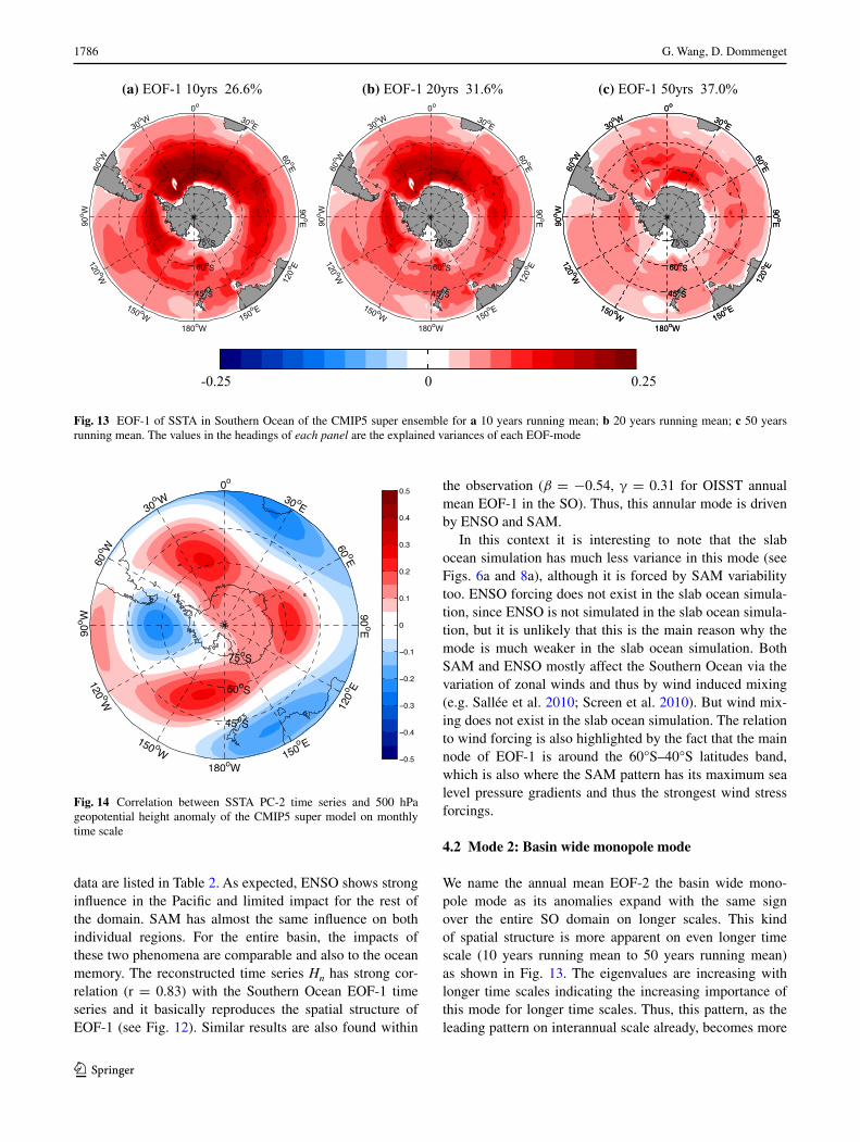
We name the annual mean EOF-2 the basin wide mono-pole mode as its anomalies expand with the same sign over the entire SO domain on longer scales. This kind of spatial structure is more apparent on even longer time scale (10 years running mean to 50 years running mean) as shown in Fig. 13. The eigenvalues are increasing with longer time scales indicating the increasing importance of this mode for longer time scales. Thus, this pattern, as the leading pattern on interannual scale already, becomes more
(a) EOF-1 10yrs 26.6% (b) EOF-1 20yrs 31.6% (c) EOF-1 50yrs 37.0%
-0.25 0 0.25
150 oW
120 oW
90o W
60o W
30o W
0o
30 oE
60 oE90
oE
120
o E
150o E
180oW
75oS
60oS
45oS150 oW
120 oW
90o W
60o W
30o W
0o
30 oE
60 oE90
oE
120
o E
150o E
180oW
75oS
60oS
45oS150 oW
120 oW
90o W
60o W
30o W
0o
30 oE
60 oE90
oE
120
o E
150o E
180oW
75oS
60oS
45oS150 oW
120 oW
90o W
60o W
30o W
0o
30 oE
60 oE90
oE
120
o E
150o E
180oW
75oS
60oS
45oS
Fig. 13 EOF-1 of SSTA in Southern Ocean of the CMIP5 super ensemble for a 10 years running mean; b 20 years running mean; c 50 years running mean. The values in the headings of each panel are the explained variances of each EOF-mode
Fig. 14 Correlation between SSTA PC-2 time series and 500 hPa geopotential height anomaly of the CMIP5 super model on monthly time scale
1787The leading modes of decadal SST variability in the Southern Ocean in CMIP5 simulations
1 3
dominant on decadal and multi-decadal scales, which is consistent with the internal centennial variability (Martin et al. 2013; Latif et al. 2013).
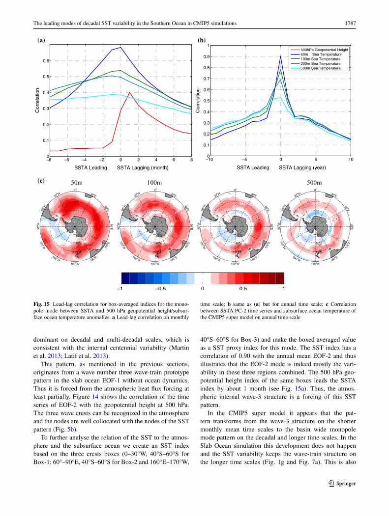
This pattern, as mentioned in the previous sections, originates from a wave number three wave-train prototype pattern in the slab ocean EOF-1 without ocean dynamics. Thus it is forced from the atmospheric heat flux forcing at least partially. Figure 14 shows the correlation of the time series of EOF-2 with the geopotential height at 500 hPa. The three wave crests can be recognized in the atmosphere and the nodes are well collocated with the nodes of the SST pattern (Fig. 5b).
To further analyse the relation of the SST to the atmos-phere and the subsurface ocean we create an SST index based on the three crests boxes (0–30°W, 40°S–60°S for Box-1; 60°–90°E, 40°S–60°S for Box-2 and 160°E–170°W,
40°S–60°S for Box-3) and make the boxed averaged value as a SST proxy index for this mode. The SST index has a correlation of 0.90 with the annual mean EOF-2 and thus illustrates that the EOF-2 mode is indeed mostly the vari-ability in these three regions combined. The 500 hPa geo-potential height index of the same boxes leads the SSTA index by about 1 month (see Fig. 15a). Thus, the atmos-pheric internal wave-3 structure is a forcing of this SST pattern.
In the CMIP5 super model it appears that the pat-tern transforms from the wave-3 structure on the shorter monthly mean time scales to the basin wide monopole mode pattern on the decadal and longer time scales. In the Slab Ocean simulation this development does not happen and the SST variability keeps the wave-train structure on the longer time scales (Fig. 1g and Fig. 7a). This is also
(b)(a)
(c) 50m 100m 500m
150 oW
120 oW
90o W
60o W
30o W
0o
30 oE
60 oE90
oE
120
o E
150o E
180oW
75oS
60oS
45oS150 oW
120 oW
90o W
60o W
30o W
0o
30 oE
60 oE90
oE
120
o E
150o E
180oW
75oS
60oS
45oS150 oW
120 oW
90o W
60o W
30o W
0o
30 oE
60 oE90
oE
120
o E
150o E
180oW
75oS
60oS
45oS150 oW
120 oW
90o W
60o W
30o W
0o
30 oE
60 oE90
oE
120
o E
150o E
180oW
75oS
60oS
45oS
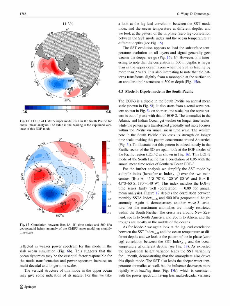
Fig. 15 Lead-lag correlation for box-averaged indices for the mono-pole mode between SSTA and 500 hPa geopotential height/subsur-face ocean temperature anomalies. a Lead-lag correlation on monthly
time scale; b same as (a) but for annual time scale; c Correlation between SSTA PC-2 time series and subsurface ocean temperature of the CMIP5 super model on annual time scale
1788 G. Wang, D. Dommenget
1 3
reflected in weaker power spectrum for this mode in the slab ocean simulation (Fig. 6b). This suggests that the ocean dynamics may be the essential factor responsible for the mode transformation and power spectrum increase on multi-decadal and longer time scales.
The vertical structure of this mode in the upper ocean may give some indication of its nature. For this we take
a look at the lag-lead correlation between the SST mode index and the ocean temperature at different depths, and we look at the pattern of the in phase (zero lag) correlation between the SST mode index and the ocean temperature at different depths (see Fig. 15).
The SST evolution appears to lead the subsurface tem-perature evolution on all layers and signal generally gets weaker the deeper we go (Fig. 15a–b). However, it is inter-esting to note that the correlation in 500 m depths is larger than in the upper ocean layers when the SST is leading by more than 2 years. It is also interesting to note that the pat-terns transforms slightly from a monopole at the surface to an annular dipole structure at 500 m depth (Fig. 15c).
4.3 Mode 3: Dipole mode in the South Pacific
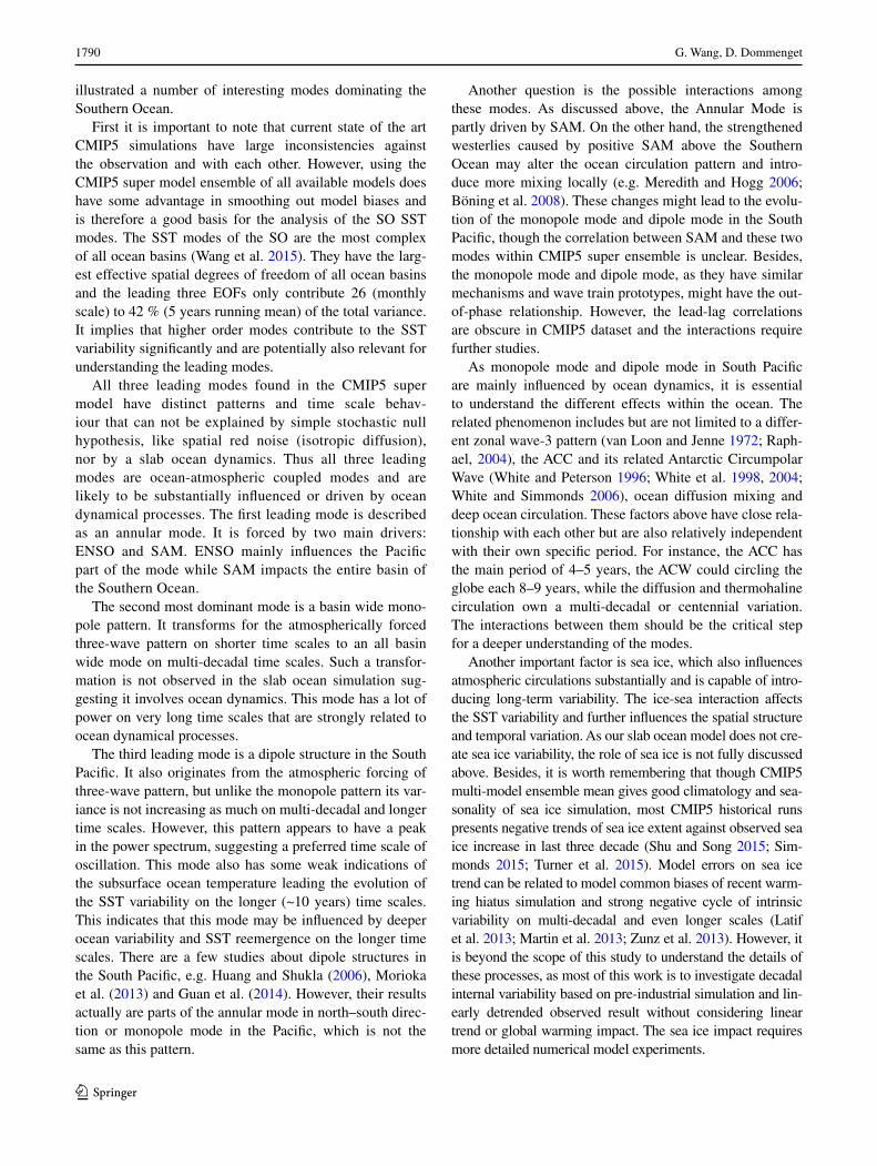
The EOF-3 is a dipole in the South Pacific on annual mean scale (shown in Fig. 5f). It also starts from a zonal wave pat-tern shown in Fig. 5c on shorter time scale, but the wave pat-tern is out of phase with that of EOF-2. The anomalies in the Atlantic and Indian Ocean get weaker on longer time scales, while the pattern gets transformed gradually and more focuses within the Pacific on annual mean time scale. The western pole in the South Pacific also loses its strength on longer time scale, making this pattern concentrate around Antarctica (Fig. 5i). To illustrate that this pattern is indeed mostly in the Pacific sector of the SO we again look at the EOF-modes of the Pacific region (EOF-2 as shown in Fig. 16). This EOF-2 mode of the South Pacific has a correlation of 0.95 with the annual mean time series of Southern Ocean EOF-3.
For the further analysis we simplify the SST mode by a dipole index (hereafter as IndexA−B) over the two main centres (Box-A: 45°S–70°S, 120°W–80°W and Box-B: 45°S–60°S, 180°–140°W). This index matches the EOF-3 time series fairly well (correlation = 0.89 for annual mean analysis). Figure 17 depicts the correlation between monthly SSTA IndexA−B and 500 hPa geopotential height anomaly. Again it demonstrates another wave-3 struc-ture, but the maximum anomalies are mostly restricted within the South Pacific. The crests are around New Zea-land, south to South America and South to Africa, and the troughs are mostly in the middle of the oceans.
As for Mode-2 we again look at the lag-lead correlation between the SST IndexA–B and the ocean temperature at dif-ferent depths and we look at the pattern of the in phase (zero lag) correlation between the SST IndexA–B and the ocean temperature at different depths (see Fig. 18). As expected the geopotential height variation leads the SST variability for 1 month, demonstrating that the atmosphere also drives this dipole mode. The SST also leads the deeper water tem-perature anomalies as well, but the influence decreases more rapidly with lead/lag time (Fig. 18b), which is consistent with the power spectrum having less multi-decadal variance
11.3%
150 oW
120 oW
90o W
60o W
30o W
0o
30 oE
60 oE90
oE
120
o E150
o E
180oW
75oS
60oS
45oS
Fig. 16 EOF-2 of CMIP5 super model SST in the South Pacific for annual mean analysis. The value in the heading is the explained vari-ance of this EOF-mode
Fig. 17 Correlation between Box [A−B] time series and 500 hPa geopotential height anomaly of the CMIP5 super model on monthly time scale

1789The leading modes of decadal SST variability in the Southern Ocean in CMIP5 simulations
1 3
than the Mode-2. However, the lag-lead relationship to the 500 m depths temperature appears to be somewhat differ-ent than in Mode-2. Here the 500 m depths temperature has stronger correlation with the SST IndexA-B when the 500 m depths temperature is leading compared to the correlations at other depths, which may suggest a deeper subsurface ocean influence on the SST IndexA−B on the longer time scales possibly via ocean reemergence. The SST pattern also has some minor changes with depth (Fig. 18c). The western pole in the Pacific gets weaker, mostly because the mixed layer depth is shallower than 100 m there in western extratropi-cal South Pacific (Dong et al. 2008), which might explain why the western pole also becomes unclear on the longer scales on the surface. In contrast, strong seasonality exists in the eastern pole region with mixed layer deeper than 200 m in austral winters (Dong et al. 2008; Sallée et al. 2013), which might lead to winter-to-winter SSTA reemergence on
interannual scale. However, there is no sufficient evidence to support the reemergence mechanism in this domain (e.g. Ciasto and Thompson 2009), which is mostly limited by the scarcity of observations. Besides, the strong correlation with ENSO/SAM obscures the relationship between SST and deeper sea temperature in the eastern pole as well.
5 Summary and discussion
In the study presented here we discussed the leading modes of SST variability in the Southern Ocean on decadal time scales in CMIP5 preindustrial scenario simulations. We compared the CMIP5 simulations with observations, sim-ple stochastic null hypothesis for the spatial structure of SST variability and against a simulation with a slab ocean that does not simulate any ocean dynamics. This study
(a)
(c)
(b)
100m 500m
150 oW
120 oW
90o W
60o W
30o W
0o
30 oE
60 oE90
oE
120
o E
150o E
180oW
75oS
60oS
45oS150 oW
120 oW
90o W
60o W
30o W
0o
30 oE
60 oE90
oE
120
o E
150o E
180oW
75oS
60oS
45oS150 oW
120 oW
90o W
60o W
30o W
0o
30 oE
60 oE90
oE
120
o E
150o E
180oW
75oS
60oS
45oS150 oW
120 oW
90o W
60o W
30o W
0o
30 oE
60 oE90
oE
120
o E
150o E
180oW
75oS
60oS
45oS
Fig. 18 Lead-lag correlation for IndicesA−B between SSTA and 500 hPa geopotential height/subsurface ocean temperature anomalies. a Lead-lag correlation on monthly time scale; b same as (a) but for
annual time scale; c Correlation between SSTA PC-2 time series and subsurface ocean temperature of the CMIP5 super model on annual time scale
1790 G. Wang, D. Dommenget
1 3
illustrated a number of interesting modes dominating the Southern Ocean.
First it is important to note that current state of the art CMIP5 simulations have large inconsistencies against the observation and with each other. However, using the CMIP5 super model ensemble of all available models does have some advantage in smoothing out model biases and is therefore a good basis for the analysis of the SO SST modes. The SST modes of the SO are the most complex of all ocean basins (Wang et al. 2015). They have the larg-est effective spatial degrees of freedom of all ocean basins and the leading three EOFs only contribute 26 (monthly scale) to 42 % (5 years running mean) of the total variance. It implies that higher order modes contribute to the SST variability significantly and are potentially also relevant for understanding the leading modes.
All three leading modes found in the CMIP5 super model have distinct patterns and time scale behav-iour that can not be explained by simple stochastic null hypothesis, like spatial red noise (isotropic diffusion), nor by a slab ocean dynamics. Thus all three leading modes are ocean-atmospheric coupled modes and are likely to be substantially influenced or driven by ocean dynamical processes. The first leading mode is described as an annular mode. It is forced by two main drivers: ENSO and SAM. ENSO mainly influences the Pacific part of the mode while SAM impacts the entire basin of the Southern Ocean.
The second most dominant mode is a basin wide mono-pole pattern. It transforms for the atmospherically forced three-wave pattern on shorter time scales to an all basin wide mode on multi-decadal time scales. Such a transfor-mation is not observed in the slab ocean simulation sug-gesting it involves ocean dynamics. This mode has a lot of power on very long time scales that are strongly related to ocean dynamical processes.
The third leading mode is a dipole structure in the South Pacific. It also originates from the atmospheric forcing of three-wave pattern, but unlike the monopole pattern its var-iance is not increasing as much on multi-decadal and longer time scales. However, this pattern appears to have a peak in the power spectrum, suggesting a preferred time scale of oscillation. This mode also has some weak indications of the subsurface ocean temperature leading the evolution of the SST variability on the longer (~10 years) time scales. This indicates that this mode may be influenced by deeper ocean variability and SST reemergence on the longer time scales. There are a few studies about dipole structures in the South Pacific, e.g. Huang and Shukla (2006), Morioka et al. (2013) and Guan et al. (2014). However, their results actually are parts of the annular mode in north–south direc-tion or monopole mode in the Pacific, which is not the same as this pattern.
Another question is the possible interactions among these modes. As discussed above, the Annular Mode is partly driven by SAM. On the other hand, the strengthened westerlies caused by positive SAM above the Southern Ocean may alter the ocean circulation pattern and intro-duce more mixing locally (e.g. Meredith and Hogg 2006; Böning et al. 2008). These changes might lead to the evolu-tion of the monopole mode and dipole mode in the South Pacific, though the correlation between SAM and these two modes within CMIP5 super ensemble is unclear. Besides, the monopole mode and dipole mode, as they have similar mechanisms and wave train prototypes, might have the out-of-phase relationship. However, the lead-lag correlations are obscure in CMIP5 dataset and the interactions require further studies.
As monopole mode and dipole mode in South Pacific are mainly influenced by ocean dynamics, it is essential to understand the different effects within the ocean. The related phenomenon includes but are not limited to a differ-ent zonal wave-3 pattern (van Loon and Jenne 1972; Raph-ael, 2004), the ACC and its related Antarctic Circumpolar Wave (White and Peterson 1996; White et al. 1998, 2004; White and Simmonds 2006), ocean diffusion mixing and deep ocean circulation. These factors above have close rela-tionship with each other but are also relatively independent with their own specific period. For instance, the ACC has the main period of 4–5 years, the ACW could circling the globe each 8–9 years, while the diffusion and thermohaline circulation own a multi-decadal or centennial variation. The interactions between them should be the critical step for a deeper understanding of the modes.
Another important factor is sea ice, which also influences atmospheric circulations substantially and is capable of intro-ducing long-term variability. The ice-sea interaction affects the SST variability and further influences the spatial structure and temporal variation. As our slab ocean model does not cre-ate sea ice variability, the role of sea ice is not fully discussed above. Besides, it is worth remembering that though CMIP5 multi-model ensemble mean gives good climatology and sea-sonality of sea ice simulation, most CMIP5 historical runs presents negative trends of sea ice extent against observed sea ice increase in last three decade (Shu and Song 2015; Sim-monds 2015; Turner et al. 2015). Model errors on sea ice trend can be related to model common biases of recent warm-ing hiatus simulation and strong negative cycle of intrinsic variability on multi-decadal and even longer scales (Latif et al. 2013; Martin et al. 2013; Zunz et al. 2013). However, it is beyond the scope of this study to understand the details of these processes, as most of this work is to investigate decadal internal variability based on pre-industrial simulation and lin-early detrended observed result without considering linear trend or global warming impact. The sea ice impact requires more detailed numerical model experiments.
1791The leading modes of decadal SST variability in the Southern Ocean in CMIP5 simulations
1 3
Acknowledgments We like to thank Dr. Claudia Frauen for fruit-ful discussions and comments. The comments of anonymous ref-erees have helped to improve the presentation of this study substan-tially. The ARC Centre of Excellence in Climate System Science (CE110001028) supported this study. The Slab Ocean model simula-tions were computed on the National Computational Infrastructure in Canberra.
References
Bayr T, Dommenget D (2014) Comparing the spatial structure of vari-ability in two datasets against each other on the basis of EOF modes. Clim Dyn 42:1631–1648
Boer GJ, Fourest S, Yu B (2001) The signature of the annular modes in the moisture budget. J Clim 14:3655–3665
Böning CW, Dispert A, Visbeck M, Rintoul SR, Schwarzkopf FU (2008) The response of the Antarctic Circumpolar Current to recent climate change. Nature Geosci 1:864–869
Bretherton CS, Widmann M, Dymnikov VP, Wallace JM, Bladé I (1999) The effective number of spatial degrees of freedom of a time-varying field. J Clim 12:1990–2009
Cai W, Watterson IG (2002) Modes of interannual variability of the southern hemisphere circulation simulated by the CSIRO climate model. J Clim 15:1159–1174
Cavalieri DJ, Parkinson CL (2008) Antarctic sea ice variability and trends, 1979–2006. J Geophys Res 113:C07004. doi:10.1029/2007JC004564
Ciasto LM, Thompson DWJ (2009) Observational evidence of reemergence in the extratropical Southern Hemisphere. J Clim 22:1446–1453
Comiso JC, Nishio F (2008) Trends in the sea ice cover using enhanced and compatible AMSR-E, SSM/I, and SMMR data. J Geophys Res 113:C02S07. doi:10.1029/2007JC004257
Cook ER, Buckley BM, D’Arrigo RD, Peterson MJ (2000) Warm-season temperatures since 1600 BC reconstructed from Tasma-nian tree rings and their relationship to large-scale sea surface temperature anomalies. Clim Dyn 16(2–3):79–91
Dommenget D (2007) Evaluating EOF modes against a stochastic null hypothesis. Clim Dyn 28(5):517–531
Dong S, Sprintall J, Gille ST, Talley L (2008) Southern Ocean mixed-layer depth from Argo float profiles. J Geophys Res 113:C06013. doi:10.1029/2006JC004051
Fyfe JC (2003) Separating extratropical zonal wind variability and mean change. J Clim 16:863–874
Gong DY, Wang SW (1999) Definition of Antarctic oscillation index. Geophys Res Lett 26:459–462
Guan Y, Zhu J, Huang B, Hu Z-Z, Kinter JL III (2014) South Pacific Ocean dipole: a predictable mode on multiseasonal time scales. J Clim 27:1648–1658
Hasselmann K (1976) Stochastic climate models Part I. Theory. Tellus 28(6):473–485
Hogg AM, Blundell JR (2006) Interdecadal variability of the South-ern Ocean. J Phys Oceanogr 36:1626–1645
Huang B, Shukla J (2006) Interannual SST variability in the southern subtropical and extra-tropical ocean. Tech Rep 223:20 pp. Center for Ocean Land Atmosphere Studies, Calverton, MD
Jones PD, Salinger MJ, Mullan AB (1999) Extratropical circulation indices in the Southern Hemisphere based on station data. Int J Climatol 19:1301–1317
Jones JM, Fogt RL, Widmann M, Marshall GJ, Jones PD, Visbeck M (2009) Historical SAM variability. Part I: century length sea-sonal reconstructions. J Clim 22:5319–5345
Karoly DJ (1989) Southern hemisphere circulation features associated with El Niño-Southern oscillation events. J Clim 2:1239–1252
Karoly DJ (1990) The role of transient eddies in low-frequency zonal variations of the Southern Hemisphere circulation. Tellus 42A:41–50
Kidson JW (1988) Indices of the Southern Hemisphere zonal wind. J Clim 1:183–194
Kidson JW, Renwick JA (2002) The Southern Hemisphere evolution of ENSO during 1981–1999. J Clim 15:847–863
Latif M, Martin T, Park W (2013) Southern Ocean sector centen-nial climate variability and recent decadal trends. J Clim 26:7767–7782
Mantua NJ, Hare SR (2002) The Pacific decadal oscillation. J Ocean-ogr 58:35–44
Martin T, Park W, Latif M (2013) Multi- centennial variability con-trolled by Southern Ocean convection in the Kiel Climate Model. Clim Dyn 40(7):2005–2022
Meredith MP, Hogg AM (2006) Circumpolar response of Southern Ocean eddy activity to a change in the Southern annular mode. Geophys Res Lett 33:L16608. doi:10.1029/2006GL026499
Mo KC, Higgins RW (1998) Tropical influences on California pre-cipitation. J Clim 11:412–430
Monselesan DP, O’Kane TJ, Risbey JS, Church J (2015) Internal cli-mate memory in observations and models. Geophys Res Lett 42:1232–1242. doi:10.1002/2014GL062765
Morioka Y, Ratnam JV, Sasaki W, Masumoto Y (2013) Genera-tion mechanism of the South Pacific subtropical dipole. J Clim 26:6033–6045
North GR, Bell TL, Cahalan RF, Moeng FJ (1982) Sampling errors in the estimation of empirical orthogonal functions. Mon Weather Rev 110:699–706
O’Kane TJ, Matear RJ, Chamberlain MA, Risbey JS, Sloyan BM, Horenko I (2013) Decadal variability in an OGCM Southern Ocean: intrinsic modes, forced modes and metastable states. Ocean Model 69:1–21
Raphael MN (2004) A zonal wave 3 index for the Southern Hemi-sphere. Geophys Res Lett 31:L23212. doi:10.1029/2004GL020365
Rayner NA, Parker DE, Horton EB, Folland CK, Alexander LV, Row-ell DP, Kent EC, Kaplan A (2003) Global analyses of sea surface temperature, sea ice, and night marine air temperature since the late nineteenth century. J Geophys Res 108:D144407. doi:10.1029/2002JD002670
Renwick JA (2002) Southern Hemisphere circulation and relations with sea ice and sea surface temperature. J Clim 15:3058–3068
Reynolds RW, Rayner NA, Smith TM, Stokes DC, Wang W (2002) An improved in situ and satellite SST analysis for climate. J Clim 15:1609–1625
Sabine CL, Feely RA, Gruber N, Key N, Lee K, Bullister JL, Wan-ninkhof R, Wong CS, Wallace DWR, Tilbrook B, Millero FJ, Peng T-H, Kozyr A, Ono T, Rios AF (2004) The oceanic sink for anthropogenic CO2. Science 305(5682):367–371
Sallée JB, Speer KG, Rintoul SR (2010) Zonnally asymmetric response of the Southern Ocean mixed-layer depth to the South-ern Annular Mode. Nature Geosci 3:273–279
Sallée JB, Shuckburgh E, Bruneau N, Meijers AJS, Bracegirdle TJ, Wang Z (2013) Assessment of Southern Ocean mixed layer depths in CMIP5 models: historical bias and forcing response. J Geophys Res Oceans 118:1845–1862. doi:10.1002/jgrc.20157
Screen JA, Gillett NP, Karpechko AY, Stevens DP (2010) Mixed layer temperature response to the Southern Annular Mode: mecha-nisms and model representation. J Clim 23:664–678
Séférian R, Iudicone D, Bopp L, Roy T, Madec G (2012) Water mass analysis of effect of climate change on air–sea CO2 fluxes: the Southern Ocean. J Clim 25:3894–3908
Shu Q, Song Z, Qiao F (2015) Assessment of sea ice simulations in the CMIP5 models. Cryosphere 9:399–409. doi:10.5194/tc-9-399-2015
1792 G. Wang, D. Dommenget
1 3
Simmonds I (2003) Modes of atmospheric variability over the South-ern Ocean. J Geophys Res 108(C4):8078. doi:10.1029/2000JC000542
Simmonds I (2015) Comparing and contrasting the behaviour of Arc-tic and Antarctic sea ice over the 35-year period 1979–2013. Ann Glaciol 56:18–28
Simmonds I, King JC (2004) Global and hemispheric climate varia-tions affecting the Southern Ocean. Antarct Sci 16(4):401–413
Taylor KE, Stouffer RJ, Meehl GA (2012) An overview of CMIP5 and the experiment design. Bull Am Meteorol Soc 93:485–498
Thompson DWJ, Wallace JM (2000) Annular modes in the extrat-ropical circulation. Part I: month-to-month variability. J Clim 13:1000–1016
Turner J (2004) Review, the El Niño southern oscillation and antarc-tica. Int J Climatol 24:1–31
Turner J, Hosking JS, Bracegirdle TJ, Marshall GJ, Phillips T (2015) Recent changes in Antarctic Sea ice. Philos Trans R Soc A 373:20140163. doi:10.1098/rsta.2014.0163
van Loon H, Jenne RL (1972) The zonal harmonic standing waves in the Southern Hemisphere. J Geophys Res 77:992–1003. doi:10.1029/JC077i006p00992
Villalba R, Boninsegna JA, Veblen TT, Schmelter A, Rubulis S (1997) Recent trends in tree ring records from high elevation sites in the Andes of northern Patagonia. Clim Change 36:425–454
Wang G, Dommenget D, Frauen C (2015) An evaluation of the CMIP3 and CMIP5 simulations in their skill of simulating the spatial structure of SST variability. Clim Dyn 44:95–114
White WB, Peterson RG (1996) An Antarctic circumpolar wave in surface pressure, wind, temperature, and sea–ice extent. Nature 380:699–702
White WB, Simmonds I (2006) Sea surface temperature-induced cyclogenesis in the Antarctic circumpolar wave. J Geophys Res 111(C8):C08011. doi:10.1029/2004JC002395
White WB, Chen SC, Peterson RG (1998) The Antarctic circumpo-lar wave: a beta effect in ocean-atmosphere coupling over the Southern Ocean. J Phys Oceanogr 28:2345–2361
White WB, Gloersen P, Simmonds I (2004) Tropospheric response in the Antarctic circumpolar wave along the sea ice edge around Antarctica. J Clim 17:2765–2779
Yuan X, Li C (2008) Climate modes in southern high latitudes and their impacts on Antarctic sea ice. J Geophys Res Oceans 113:C06S91
Yuan X, Yonekura E (2011) Decadal variability in the Southern Hemi-sphere. J Geophys Res 116:D19115. doi:10.1029/2006JC004067
Zunz V, Goosse H, Massonnet F (2013) How does internal variability influence the ability of CMIP5 models to reproduce the recent trend in Southern Ocean sea ice extent? Cryosphere 7:451–468. doi:10.5194/tc-7-451-2013


