Department of Mathematical Sciences
MSc. in Modern Applications of Mathematics
The Dynamics of Crowds
Gareth William Parry
Supervisors: Prof. C. J. Budd & Dr. C. J. K. Williams
September 2007
i
Abstract
Crowds pose an interesting example of a complex system in which emergent behaviour is
observed out of the interaction of many individual agents. This behaviour can be very
important in the safe design of sports and other stadia, especially in the case of possible
emergency situations. For this reason crowd dynamics is of great interest to architects.
The purpose of this project is to review the current literature on crowd dynamics and to
look at some simulations of different types of crowd behaviour in certain specific
situations namely: the meeting of two crowds in a ’scramble crossing’, the motion of a
crowd though an exit and the response of a crowd to an emergency (such as a fire). The
student will implement a differential equation model of the crowd crossing problem. In
particular, they will study the emergent behaviour that arises in the scramble crossing
problem and see how this depends on various parameters relating to the individual actions
of the members of the crowd.
Declaration: I hereby certify that the work in this document is my own, unless otherwise
referenced.
Signed ............................................................ Gareth Parry
ii
Acknowledgements
I would like to thank Professor Budd in particular for his help and input whilst writing
this thesis. The lively debate and insightful questions raised in our meetings was one of
the particularly enjoyable aspects of the project. I would also like to thank Dr Chris
Williams and Odysseas Kontovourkis for their help in providing an Architects insight
into pedestrian dynamics.
Movies and Code
Submitted along with this thesis are copies of several movies created by the simulator and
converted to *.avi files. Also included on the CD are the final MATLAB script and
function files (hard copies are in Appendix A) along with several *.mat files which are
saved data from different simulations. The movie and *.mat files are named with the
number of pedestrians simulated followed by the geometry the flow was simulated in. So
if 500 pedestrians were modelled in a Scramble Crossing then the associated files would
be: Movie: 500scramblecrossing.avi
Data: 500scramblecrossing.mat
Finally a *.PDF version of this thesis is also provided for submission to a plagiarism
prevention website.
iii
Contents
Introduction....................................................................................................................... 1
An Overview of Models for the Simulation of Pedestrian Dynamics........................... 3
2.1 Pedestrian Modelling approaches ............................................................................. 4
2.2 The Gas-Kinetic Model of Pedestrian Flows............................................................ 5
2.3 The Magnetic Force Model....................................................................................... 9
2.4 Queuing Systems .................................................................................................... 12
2.5 Cellular Automata................................................................................................... 18
2.6 The Social Force Model.......................................................................................... 22
2.6.1 The Driving Force............................................................................................ 23
2.6.2 Pedestrian Interactions ..................................................................................... 24
2.6.3 Boundary Interactions...................................................................................... 27
2.6.4 Attractive Interactions...................................................................................... 27
2.6.5 Individuality and Random Behaviour Fluctuations ......................................... 28
2.6.6 Another Formulation........................................................................................ 28
Self-Organisation Phenomena in Pedestrian Flows..................................................... 30
3.1 Intersecting Flows................................................................................................... 30
3.2 Bottlenecks.............................................................................................................. 31
3.3 Lane Formation....................................................................................................... 31
3.4 Shockwaves............................................................................................................. 32
Implementation of the Social Force Model................................................................... 33
4.1 Numerical Solution of the Social Force Model ...................................................... 33
4.2 The Desired Destination and Waypoints ................................................................ 37
4.3 The Desired Velocity .............................................................................................. 39
Simulation and Analysis of the Social Force Model .................................................... 41
5.1 The Model Constants .............................................................................................. 41
5.2 Pedestrian Counterflows ......................................................................................... 44
5.3 A Ninety Degree Corner ......................................................................................... 47
5.4 The Scramble Crossing ........................................................................................... 51
5.5 Model Shortcomings............................................................................................... 54
Summary and Future Directions................................................................................... 56
iv
Bibliography .................................................................................................................... 58
Appendix A...................................................................................................................... 59
MATLAB Codes.............................................................................................................. 59
A.1 SFMDFPIBI.m....................................................................................................... 59
A.2 fun5.m ...........................................................................................................................................63
v
List of Figures
Figure 1: Acceleration force A acting on a to avoid collision with b............................... 12
Figure 2: Planar Graph ( ),G V E′ ′ ′ and dual graph ( ),G V E ............................................ 14
Figure 3: Lane switching behaviour in Blue/Adler model................................................ 21
Figure 4: Emerging Lane Formation................................................................................. 21
Figure 5: Distance between and α β ............................................................................... 25
Figure 6: Fαβ characterises anisotropic behaviour ............................................................ 26
Figure 7: Striping phenomena in Intersecting flows......................................................... 30
Figure 8: illustration of pedestrian behaviour causing shockwaves ................................. 32
Figure 9: Cputime for several solvers ............................................................................... 34
Figure 10: Verlet - Sphere................................................................................................. 35
Figure 11: Pedestrian paths with a single point for p�
, desired destination ...................... 37
Figure 12: Pedestrian paths using a desired destination array .......................................... 37
Figure 13: Pedestrians path with and without a waypoint ................................................ 38
Figure 14: The difference between a fixed desired velocity and a variable one............... 40
Figure 15: An example of pedestrian flows in the test room (Not to Scale) .................... 42
Figure 16: The initial and final pedestrian positions created for a counterflow ............... 45
Figure 17: These figures show how flow oscillates at a bottleneck ................................. 46
Figure 18: The Speed of a single Pedestrian around a ninety degree corner .................... 47
Figure 19: The simulation of a ninety degree corner ........................................................ 48
Figure 20: The overall mean speed of pedestrians around a ninety degree corner........... 49
Figure 21: Plots of the speed characteristics of a Scramble crossing ............................... 51
Figure 22: Variance and Standard Deviation of Pedestrian in a Scramble Crossing........ 52
Figure 23: Regions where Lattice Constants are calculated..............................................53
Figure 24: The New Verlet-Sphere................................................................................... 55

vi
List of Tables
Table 1: Simulation Parameters ........................................................................................ 43
Table 2: Lattice Constants ................................................................................................ 54
1
Chapter 1
Introduction
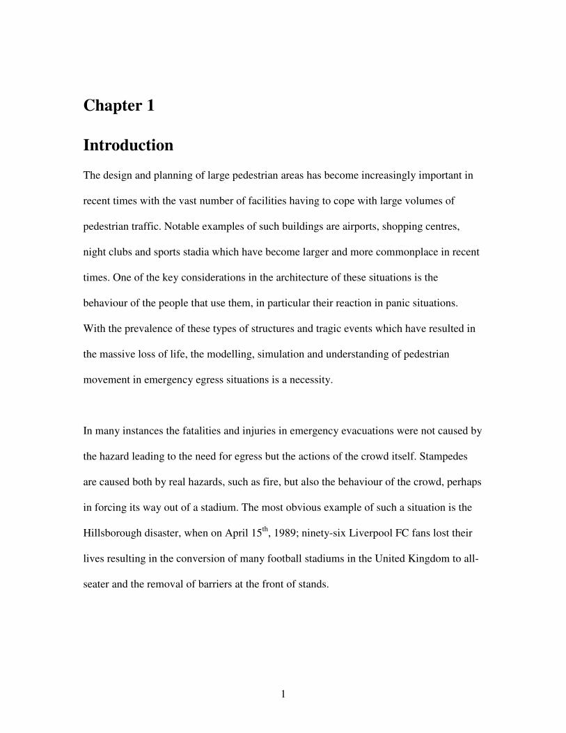
The design and planning of large pedestrian areas has become increasingly important in
recent times with the vast number of facilities having to cope with large volumes of
pedestrian traffic. Notable examples of such buildings are airports, shopping centres,
night clubs and sports stadia which have become larger and more commonplace in recent
times. One of the key considerations in the architecture of these situations is the
behaviour of the people that use them, in particular their reaction in panic situations.
With the prevalence of these types of structures and tragic events which have resulted in
the massive loss of life, the modelling, simulation and understanding of pedestrian
movement in emergency egress situations is a necessity.
In many instances the fatalities and injuries in emergency evacuations were not caused by
the hazard leading to the need for egress but the actions of the crowd itself. Stampedes
are caused both by real hazards, such as fire, but also the behaviour of the crowd, perhaps
in forcing its way out of a stadium. The most obvious example of such a situation is the
Hillsborough disaster, when on April 15th
, 1989; ninety-six Liverpool FC fans lost their
lives resulting in the conversion of many football stadiums in the United Kingdom to all-
seater and the removal of barriers at the front of stands.
2
The key aim of this thesis is to explore the current theories and models relating to
pedestrian flows and implement two of these schemes. There is a massive breadth of
literature relating to such models which have been developed over the last forty years.
The model this thesis will focus on and implement is the Social Force Model which was
developed D. Helbing and P. Molnár[1],[2].
The ultimate aim of this is to explore the emergent behaviour of pedestrian systems,
particularly in the case of a scramble crossing and the expected striping effects. Other
models will be discussed and outlined in some detail to highlight the variety of theories
suggested to simulate pedestrian dynamics. The scheme proposed by V. J. Blue and J. L.
Adler, their Cellular Automata[3] model, will be explored in some detail as initially it
was intended that this model also be implemented in the MSc project.
3
Chapter 2
An Overview of Models for the Simulation of Pedestrian
Dynamics
The simulation of pedestrian movement has being explored in a variety of ways. In this
chapter the aim will be to provide an outline of the most prominent of these models along
with an exposition of the governing equations of each scheme. In general these models
describe the forces each pedestrian feels; treating each pedestrian as a particle in a larger
system and using Newton’s Second Law to evaluate position, velocity and acceleration.
A numerical solver then can be used over a discrete timestep providing a velocity and
position update. One of the key differences between pedestrian traffic models and other
roadway-based traffic systems is that pedestrian locations are not restricted to a single
dimension. Whilst many of the models are initially based on vehicle traffic systems, these
are only one dimensional models and unlike pedestrian movement subject to a number of
laws and restrictions governing traffic. Pedestrian movement is inherently more
changeable than that of vehicles, as unlike vehicle flow which is controlled by well
defined lane markings with lane change and passing opportunities restricted, there are no
such restrictions on pedestrian walkways. Pedestrian interaction is also markedly
different to that of cars since safety concerns are much less, clearly pedestrians can
actually touch each other without incident, which is certainly not true of moving vehicles.
Also pedestrians often move in pair or clusters, such as couples or family groups, whilst
such attractive influences are rare in vehicle traffic. This leads to interactions between
people that have to be considered in any model, examples of which are bumping into
4
each other, exchange of places or bypass when pedestrian density is high as opposed to
sidestepping which would be analogous to the behaviour of a car. The velocity and
acceleration characteristics of pedestrians are also very different, with each pedestrian
having their own desired and maximum speeds. They are also able to accelerate to full
speed from standstill almost immediately and can change speed more rapidly allowing
them to take advantage of gaps in traffic when they arise.
2.1 Pedestrian Modelling approaches
Pedestrian flow models can be classified in different ways depending upon how the
scheme treats the pedestrians and the level of detail of the models. These classifications
are:
1. Microscopic models, which consider individual pedestrian behaviour separately.
The pedestrian behaviour in these models is often described by their interactions
with other pedestrians in the system.
2. Mesoscopic models, which do not consider each pedestrian individually but the
overriding characteristics, such as velocity distributions. The pedestrian behaviour
is described microscopically though not specifically but rather in terms of velocity
distributions.
3. Macroscopic models, which do not make distinctions between individual
pedestrians nor describe their individual behaviour but consider the flow in terms
of density, average velocity and flow patterns.
As previously discussed, the main focus of this thesis will be on the Social Force Model
and Cellular Automata which are both examples of microscopic models. Whilst these are
5
computationally demanding, both the individual and emergent group behaviour of
pedestrians is of interest.
2.2 The Gas-Kinetic Model of Pedestrian Flows
This model was first suggested by L. F. Henderson[4], who treats large pedestrian crowds
like molecules in a dilute gas. Whilst there are some seemingly random fluctuations in the
movements of people in large crowds, the fact that each individual has a mass and
velocity suggests that the classical Maxwell-Boltzmann statistics could be used to
describe the motion of a crowd using a density function ( ), ,f x v t� �
. Henderson only
applies the Maxwell-Boltzmann equations to the so called gaseous phase. This is when
the crowd is moving and has a low particle density, defined as the number of persons per
unit area. If this is small then each individual is assumed to be able to move at their
desired speed. However the model becomes problematic when boundary interactions
occur and particle density increases, for example at a doorway. This is described as a
phase transformation to a densely packed crowd liquid phase. To describe the crowd gas
several assumptions are made, firstly that movement takes place on a continuous plane
and that at time t each of the N pedestrians has a position (x,y) and velocity (Vx,Vy).
Secondly the crowd is considered to be homogeneous, that is each particle will have the
same mass and probability of velocity components. This homogeneity is analogous to
chemical purity in molecular systems, although Henderson suggests that this
homogeneity may not be a fair assumption due to what he describes as sexual
inhomogeneity, the idea that men and women behave differently in crowds. This
nonuniformity may extend beyond gender and also be attributed to other social and
environmental factors such, as the age of each pedestrian. The next assumption is that the
6
particles are independent of each other in position and velocity components with position
and velocity of the individual pedestrian being uncorrelated. Finally, the crowd is
assumed to be in equilibrium and that it can be treated as a statistical ensemble of any
individual. The Maxwell-Boltzmann equations for the described assumptions are as
follows, with the probability density function P(Vx), for a single fluctuating velocity
component, Vx, is
( )2
2
. .. .
1 1 1exp
22
xv xx
x r m sr m s
dN VP V
N dV vvπ
� �≡ = −� �
� � (2.2.1)
Where . .r m sv is the standard deviation of the speed v V≡ . The expression for Vy is
analogous and can be combined to get the resultant velocity, V
( )2
2 2
. . . .
1 1 1exp
2 2
V
r m s r m s
dN VP V
N dV v vπ
� �≡ = −� �
� � (2.2.2)
With the probability density function for speed
( )2 2
. .2 2
1exp with / 2
4 4
vr m s
dN v vP V v v
N dv v v
π ππ
� �≡ = − =� �
� � (2.2.3)
These functions can be extended to situations where there may be a superimposed flux
upon the system, for instance a crowd moving along a corridor. (2.2.1) Is shifted in this
case with a new velocity component x x x
V V V′ ≡ −
( )2
2
. .. .
1 1 1exp
22
xV xx
x r m sr m s
dN VP V
N dV vvπ
′ � �′′ ≡ = −� �
′ � � (2.2.4)
With analogous treatment of (2.2.2) and (2.2.3).
Clearly this is a somewhat simplistic view of pedestrian dynamics, but it is the starting
point for S. Hoogendoorn and P. H. L. Bovy’s formulation [5]. In the simplest case where
7
there is no distinction between pedestrian types, the gas-kinetic equations represent
describe the dynamics of the generalised phase-space density ( ), , ,t x v wρ ρ= defined
by ( ) ( ), , | ,r t x f v w t x . Here ( ),r t x is a multidimensional density which reflects the
expected number of traffic entities per unit volume at ( ),t x , with ( ), | ,f v w t x the joint
probability density function of the velocity v and continuous attributes w which reflects
characteristics of traffic flow and its constituent entities such as desired velocity. The gas-
kinetic equation in n dimensions is
( )
( )
( )
( )
( )
( )( ) ( )
. . .
IV VI II III
x v w
event cond
v A Bt t t
ρ ρ ρρ ρ ρ
∂ ∂ ∂� � � �+ ∇ + ∇ + ∇ = +� � � �
∂ ∂ ∂� � � �
����� ���������� ����� �����
(2.2.5)
This equation shows how the phase-space density changes, with term (I) being
convection, (II) acceleration, (III) the adaptation of continuous attributes, (IV) event
based noncontinuum processes and (V) the condition-based noncontinuum processes. The
so-called pedestrian phase-space density (P-PSD – this is consistent with Hoogendoorn’s
notation) ( ), , ,t x v wρ conforms to the setup laid out in the introduction to this chapter,
that is it is a two dimensional system to describe the pedestrian flow where each
pedestrian may have different velocity, desired velocity and acceleration considerations.
With this in mind, pedestrian density ( ),r x is defined to be the expected number of
pedestrians per unit area.
In (2.2.5) terms (I) – (III) are the continuum processes, that is they are smooth and
describe the change in the spatial distribution of the pedestrians (in terms of density).
They represent continuous changes in the independent variables , , x v w . Terms (IV) and
8
(V) describe the noncontinuum processes of pedestrian interaction – Hoogendoorn calls
this a stimulus-response mechanism: “an event causes a remedial manoeuvre of the
impeded pedestrian” and as such aren’t continuous but occur when pedestrians engage
with each other. The current research omits terms (III) and (V). The resulting equation to
describe the P-PSD is
( ) ( )
( )
( ) ( )
( ) ( )
1 2 1 2
1 2 1 2
IVI II
event event
v v A At x x v v t t
ρ ρ ρρ ρ ρ ρ
+ −∂ ∂ ∂ ∂ ∂ ∂ ∂� � � �
+ + + + = +� � � �∂ ∂ ∂ ∂ ∂ ∂ ∂� � � �
������������������ ���������
(2.2.6)
With 1 2 and A A describing the acceleration laws of the system and the terms in (IV)
describing noncontinuum events which increase or decrease the phase-space density
respectively. Hoogendoorn and Bovy describe in detail the derivation of each term,
however it is sufficient for this thesis to describe the model in general without detailing
specifics.
One area of interest in the derivation however is the role of transition probabilities in the
pedestrian interactions, as these probabilities describe how the pedestrian’s direct
environment affects their behaviour. Three types of pedestrian interaction are
distinguished, which correspond to the stimulus-response mechanisms:
1. One-sided interaction – where pedestrian p catches up to a slower moving
pedestrian q. Here p is held up by q but the converse isn’t true.
2. Two-sided interaction – where two pedestrian travelling in opposite directions
meet head on and hold each other up.
9
3. Passive interaction – this is the same as 1 except the pedestrian being considered
is the one being caught up and so will not take any action as their progress is
unimpeded.
Transition probabilities are then used to describe the expected behaviour of each
pedestrian in the system in one of the three interactions described.
The model also touches on factors that are relevant in several models, particularly the
pedestrian’s spatial requirements and different classes of pedestrian. The Gas-Kinetic
model traditionally assumes that the particles in the system are infinitesimally small, this
however is not necessarily a valid assumption for modelling pedestrian flows since the
amount of space each pedestrian occupies is of dominant importance. The pedestrian
classification is the same problem Henderson touched on, in that gender, age or other
demographic characteristics may affect the behaviour of individuals in the system.
Hoogendoorn and Bovy then solve the formulated problem using the Monte Carlo
method in a variety of simple cases such as unidirectional, bidirectional and crossing
pedestrian flows. Their results are reasonable and reproduce the expected velocity-density
relations qualitatively.
2.3 The Magnetic Force Model
The next model was developed by S. Okazaki and S. Matsushita[6] and as the title
suggests treats the pedestrians within the system as charged objects within the resulting
magnetic field. Each pedestrian in the system is given a positive charge and destinations
such as doorways or service counters a negative charge. Clearly the attractive nature of
10
opposite magnetic charges results in the pedestrians moving towards these destination
points. This magnetic effect also means that pedestrians exert a repulsive force upon each
other which physically corresponds to them avoiding collisions with each other and
objects such as boundaries.
Once the room has been setup, it is inputted as a series of vertexes described in the
Cartesian coordinates. With the destination details configured the model then requires a
detailed amount of input data to produce realistic results before the simulation can be
started. The required data is the desired destination, initial position, initial velocity, the
pedestrian orientation, time that the pedestrian starts walking and their method of walk.
This final input is the most interesting as the simulation can implement a wayfinding
technique where the pedestrians will follow a sequence of points (corners in the case of
this simulator) until they have an unobstructed route, that is no boundaries in their path,
to their desired destination. Another point of interest in this model is the velocity input,
which is a maximum velocity. This is simply because if there were no upper bound on the
velocity the pedestrians would accelerate without limit according to Coulomb’s Law.
Since the pedestrians are treated as magnetic objects, the appropriate force law is
Coulomb’s Law
1 2
2
.1
4
Q QF
sπε= (2.3.1)
1 2 and Q Q are the signed values for the magnetic charge of the objects they represent, s is
the distance between the two particles and k, the so called Coulomb constant, is the
constant term 14πε . If 1Q represents a positively charged pedestrian, a, say and 2Q a
11
negatively charged pole representing the desired destination. Since a two dimensional
setup is being considered the force is a vector quantity resulting in the following form of
Coulomb’s Law
1 2
3
.ˆ. .
Q QF k
s= s (2.3.2)
Here s is the unit vector pointing from 1 2 to Q Q . If the charges have the same sign, as in a
pedestrian-pedestrian interaction, then the resulting force is positive which corresponds to
a repulsive interaction. Conversely if the signs are different, in the case of a pedestrian-
destination interaction, there is a negative force and so an attractive force is felt which
leads to the particle accelerating towards the destination. When more than two charges
are present in the system the forces are superimposed, that is the force between any pair is
the sum of all the exerted forces from the component charges.
The model also incorporates another force which acts upon the pedestrians in order to
simulate the collision avoidance characteristics of the crowd. If two pedestrians come
within a certain distance of each other then the new force is exerted upon the pedestrians.
That is, if a, intersects within a specific area of another pedestrian then a feels the
following repulsive force and resulting acceleration to cause a change of direction and
thus preventing a collision. This acceleration is represented by
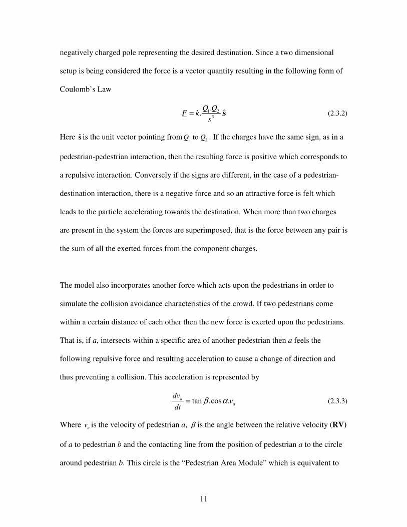
tan .cos .aa
dvv
dtβ α= (2.3.3)
Where a
v is the velocity of pedestrian a, β is the angle between the relative velocity (RV)
of a to pedestrian b and the contacting line from the position of pedestrian a to the circle
around pedestrian b. This circle is the “Pedestrian Area Module” which is equivalent to
12
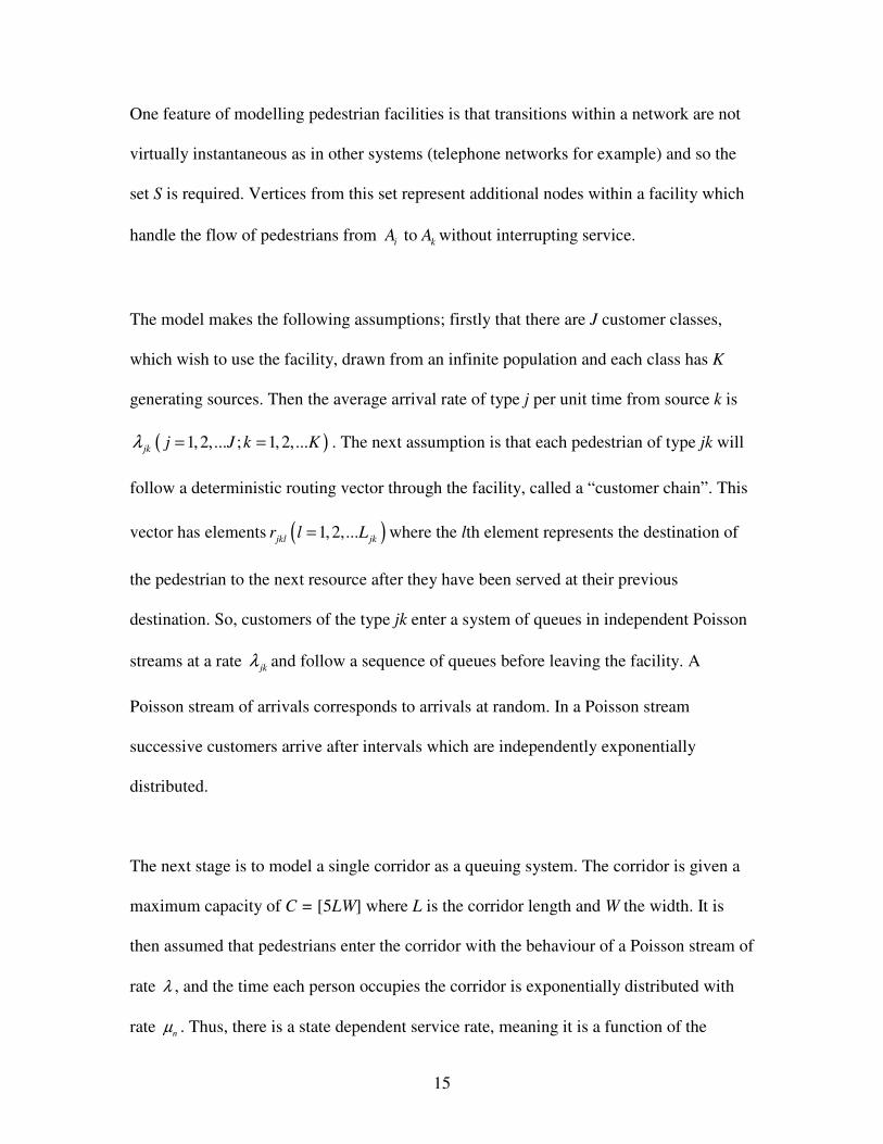
the “Territorial Sphere” in Helbing’s Social Force Model [1]. Finally α is the angle
between relative velocity of pedestrian a (RV) to the pedestrian b and the velocity of
pedestrian a.
Figure 1: Acceleration force A acting on a to avoid collision with b
This model was used to simulate to simulate an escape from fire on one floor of an office
building, to plot the movement of pedestrians in part of an underground railway station
and pedestrian flows in a hotel lobby. The model can be used to evaluate how long an
emergency escape might take, the behaviour of pedestrians in queuing situations – that is
the number in each queue, the length of their wait and movement processes.
2.4 Queuing Systems
Queuing theory, which is generally considered to be a branch of operations research,
describes pedestrian flows in terms of probability functions. The pedestrian will arrive at
A
13
a given node, which represents a server, with a certain probability. They will then spend a
certain amount of time being served, at a shop till for example, and then continue on to
their next destination, leaving the queue. A queuing system is comprised of three
elements, the pedestrian’s arrival in the queue, the service mechanism and the service
discipline. A queuing discipline determines the manner in which the exchange handles
calls from customers. Examples are
• First In, First Out – This principle states that customers are served one at a time
and that the customer that has been waiting longest is served first
• Last In First Out – This principle also serves customers one at a time, however
the customer with the shortest waiting time will be served first
• Processor Sharing – Customers are served equally. Network capacity is shared
between customers and they all effectively experience the same delay
Queuing is handled by control processes within exchanges, which can be modelled using
state equations. Queuing systems use Markov Chains which model the system in each
state where Incoming traffic to these systems is modelled via a Poisson distribution. The
stochastic process in a queuing system is the population of a particular room.
The first model to be discussed was formulated by S. J. Yuhaski, Jr and J. Macgregor
Smith[7] which develops a state dependent queuing model for the congestion effects of
movement through circulation systems of a building. Circulation systems are, in this case,
the pathways of movement such as corridors, stairways and ramps. The problem they
describe is that of crowded pedestrian flows in confined spaces and the paper describes
the following as “crucial aspects to movement Systems”
14
1. The service rate of the movements system decays with increasing traffic
2. The amount of available space within the movement system is finite
These characteristics are the basis for the construction of their model and their aim to
“best capture the congestion effects”. The first step is to generate a representation for the
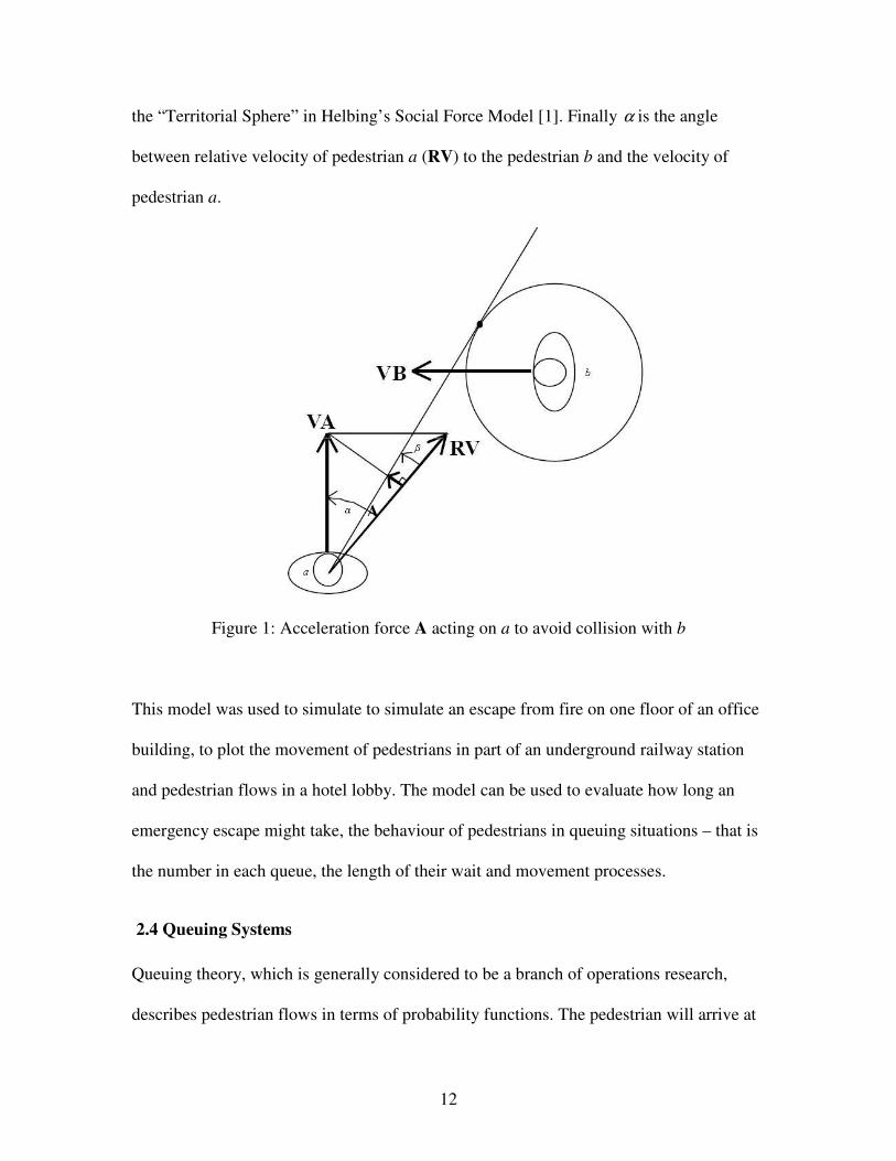
facility; this is its floor plan. This can be represented by a planar graph ( ),G V E′ ′ ′ (this is
consistent with their notation) and so the queuing network is the Dual Graph ofG′ . There
are then two distinct types of spatial entity which must be distinguished, that is the
activity network and the circulation network. So V is partitioned into two sets { },V A S= .
The set { }1 2, ,..., NA A A A= is the set of activity nodes which represent so called “activity
areas”, say a department of a shop. The set { }1 2, ,..., MS S S S= then is the circulation
nodes which are the movement pathways joining activity areas.
Figure 2: Planar Graph ( ),G V E′ ′ ′ and dual graph ( ),G V E
15
One feature of modelling pedestrian facilities is that transitions within a network are not
virtually instantaneous as in other systems (telephone networks for example) and so the
set S is required. Vertices from this set represent additional nodes within a facility which
handle the flow of pedestrians from to i k
A A without interrupting service.
The model makes the following assumptions; firstly that there are J customer classes,
which wish to use the facility, drawn from an infinite population and each class has K
generating sources. Then the average arrival rate of type j per unit time from source k is
( )1,2,... ; 1,2,...jk j J k Kλ = = . The next assumption is that each pedestrian of type jk will
follow a deterministic routing vector through the facility, called a “customer chain”. This
vector has elements ( )1,2,...jkl jk
r l L= where the lth element represents the destination of
the pedestrian to the next resource after they have been served at their previous
destination. So, customers of the type jk enter a system of queues in independent Poisson
streams at a rate jk
λ and follow a sequence of queues before leaving the facility. A
Poisson stream of arrivals corresponds to arrivals at random. In a Poisson stream
successive customers arrive after intervals which are independently exponentially
distributed.
The next stage is to model a single corridor as a queuing system. The corridor is given a
maximum capacity of C = [5LW] where L is the corridor length and W the width. It is
then assumed that pedestrians enter the corridor with the behaviour of a Poisson stream of
rate λ , and the time each person occupies the corridor is exponentially distributed with
rate n
µ . Thus, there is a state dependent service rate, meaning it is a function of the
16
number of pedestrians in the corridor. The model now uses the Chapman-Kolmogorov
steady-state difference equations for the state probabilities 1 2, ,...,c
p p p
0 1 10
1 2
...
...
nn
n
p pλ λ λ
µ µ µ−= (2.4.1)
Such that
0 1 1
10 1 2
...11
...
Cn
n np
λ λ λ
µ µ µ−
=
� �= +
� � (2.4.2)
Here the arrival rates are not influenced by the number in the queue so
0 1 ...C
λ λ λ λ= = = = . The paper suggests two congestion models with approximate
overall walking-speed n
V , firstly the linear relation
( )1.5
1n
V C nC
= + − (2.4.3)
Or the exponential relation, which may be more accurate, is
1
expn
nV A
γ
β
� �� �−= − � �
� � � � (2.4.4)
A is the amplitude with parameters and β γ are called the scale and shape parameters. In
both models the service raten
r , is the average of the inverse of the time it takes for the
pedestrians to travel the length of the corridor
nn
Vr
L= (2.4.5)
With overall service rate
n n
nrµ = (2.4.6)
The overall service rate for the linear model then becomes
17
( )1.5
1n
C nC
µ = + − (2.4.7)
Then the Chapman-Kolmogorov equations become
( )0
1
1
nn n n
i
p pA
C i iLC
λ
=
=� �
− +� �� �
∏ (2.4.8)
And
( )10
1
11
1
nC
nn
i
k
pC i i=
=
= +
− +
∏ (2.4.9)
With n LCA
k λ= . Similarly the Chapman-Kolmogorov equations for the exponential model
are
0
1
1exp
nn
n
i
p p
A ii
L
γ
λ
β=
=� �� �� �−� �� �
− � �� � � �� � � � � �� �� �
∏
(2.4.10)
And
10
1
11
1exp
Cn
nn
i
p A ii
L
γ
λ
β
=
=
� �� �� �
= + � �� �� �−� �� �− � � � �� �� � � � � �� �
∏
(2.4.11)
Another notable Queuing Model is the one developed by Løvas[8] introduced a similar
stochastic model where pedestrians can be modeled in a queuing network. This model is
setup similarly where Nodes in the network represent rooms and links the doors. Each
pedestrian will then select a new node with a given probability. The model can evaluate
several performance measures such as the mean number of persons in a node and the
mean number of safe evacuees. Løvas has developed a tool called EVACSIM which has
18
simulated egress in several different setups. The system visualizes the movement of the
pedestrians and provides qualitative information about behaviour at bottlenecks in the
queuing systems.
2.5 Cellular Automata
A cellular automaton is a discrete model studied in computability theory, mathematics,
and theoretical biology. It consists of a regular grid of cells, each in one of a finite
number of states. Time is discretised and the state of a cell at time t is a function of the
states of a finite number of cells (called its neighbourhood) at time t − 1. These
neighbours are a selection of cells relative to the specified cell, and do not change
(though the cell itself may be in its neighbourhood, it is not usually considered a
neighbour). Every cell has the same rule for updating, based on the values in this
neighbourhood. Each time the rules are applied to the whole grid a new generation is
created. The Cellular Automata method can be used to simulate pedestrian flow. It is fast
and relatively simple, with the walkway represented by a cellular grid. In this
representation each cell within the grid is occupied by one pedestrian. The pedestrian
flow is modelled by a set of governing rules which differ according to the particular
model being considered.
The most notable Cellular Automata model is the one developed by V. J. Blue and J. L.
Adler ([3],[9]) which models the walkway as a circular lattice (closed loop) with width
W, length G and class L = WG. Each cell within the lattice is assigned a label
( ),L i j with1 and 1i W j G≤ ≤ ≤ ≤ . The density of pedestrians on the walkway is
determined at the start of the simulation and remains constant throughout. The
19
Microsimulation continues in discrete timesteps for 1,2,...,i
t i T= . The lane assignments
and speed updates change the position of all the pedestrians within the lattice in four
stages determined by the local rules which are applied to each individual on the walkway.
The stages are
1. A set of lane change rules determining the lane for each pedestrian on the lattice
2. The pedestrians are moved in to the assigned lanes
3. A set of rules is applied to find the allowable speed of each pedestrian based on
the available gap ahead and the pedestrians desired speed
4. Forward movements based on the allowed speeds are made
The rule sets for each stage are
Lane Change (parallel update 1 – stages 1 and 2)
1) Eliminate conflicts: If two walkers are adjacent then they cannot sidestep into each
other
a) If a cell is available between two walkers then assign it to one of then with a
50/50 split
2) Identify gaps: The lane (same or left/right adjacent) is chosen which best advances
forward movement upto v_max according to the gap computation subprocedure that
follows the step forward update
a) For Dynamic Multiple Lanes (DML):
i) Step out of lane if a walker in the opposite direction is within 8 cells by
assigning gap = 0
ii) Step behind a pedestrian moving in the same direction when avoiding a
collision with an oncoming walker by choosing any available lane with
gap_same = 1 when gap = 1
b) Ties of equal maximum gaps ahead are resolved according to:
i) If the 2-way tie is between adjacent lanes then a 50/50 split between which
lane is chosen
ii) If the 2-way tie is between the current and an adjacent lane then the walker
stays in lane
iii) If there is a 3-way tie between the current and adjacent lanes then the
pedestrian stays in lane
20
3) Move (this is stage 2): Each pedestrian n
p is moved 0, +1 or -1 lateral sidesteps after
1) – 3) is completed
Step forward (parallel update 2 – stages 3 and 4)
1) Update velocity: Let ( )nv p gap= where gap is from the subprocedure below
2) Exchanges: IF gap = 0 or 1 AND gap = gap_opp (cell occupied by an opposite
moving pedestrian) THEN with probability p_exchg,
( ) 1nv p gap= + ELSE ( ) 0nv p = . That is the walker and the opposite moving
pedestrian either exchange cells with a predefined probability p_exchg or stop when
they meet each other and sidestep at the next timestep
3) Move (this is stage 4): each pedestrian n
p is moved ( )nv p cells forward
Gap Computation Subprocedure
1) Same direction: Look ahead a up to 8 cells (8 = 2* the largest v_max) IF an occupied
cell is found with a pedestrian moving in the same direction THEN set gap_same to
the number of cells between the two pedestrians ELSE set gap_same = 8 2) Opposite Direction: IF an occupied cell is found with an opposite moving pedestrian
THEN set gap_opp to (0.5*number of cells between the pedestrians) ELSE gap_opp
= 4
3) Assign gap = MIN(gap_same, gap_opp, v_max)
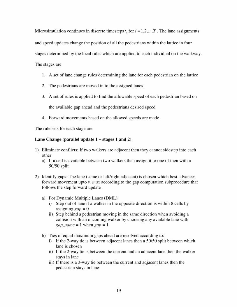
The lane switching procedure is illustrated in Figure 3. For pedestrian 1, the adjacent
cells on both the left and right are available. The unoccupied distance on however is
uniquely maximal in the present lane so no switch is required. Pedestrian 4 conflicts to
the right with pedestrian 6 and in this instance pedestrian 6 is given access to this cell,
hence 4 can only sidestep to the left. The unoccupied distance is largest in this lane and
so 4 will switch. The change is represented by 4’. Pedestrian 7 cannot switch lanes since
both adjacent lanes are occupied and thus the lane change procedure is terminated.
21
Figure 3: Lane switching behaviour in Blue/Adler model
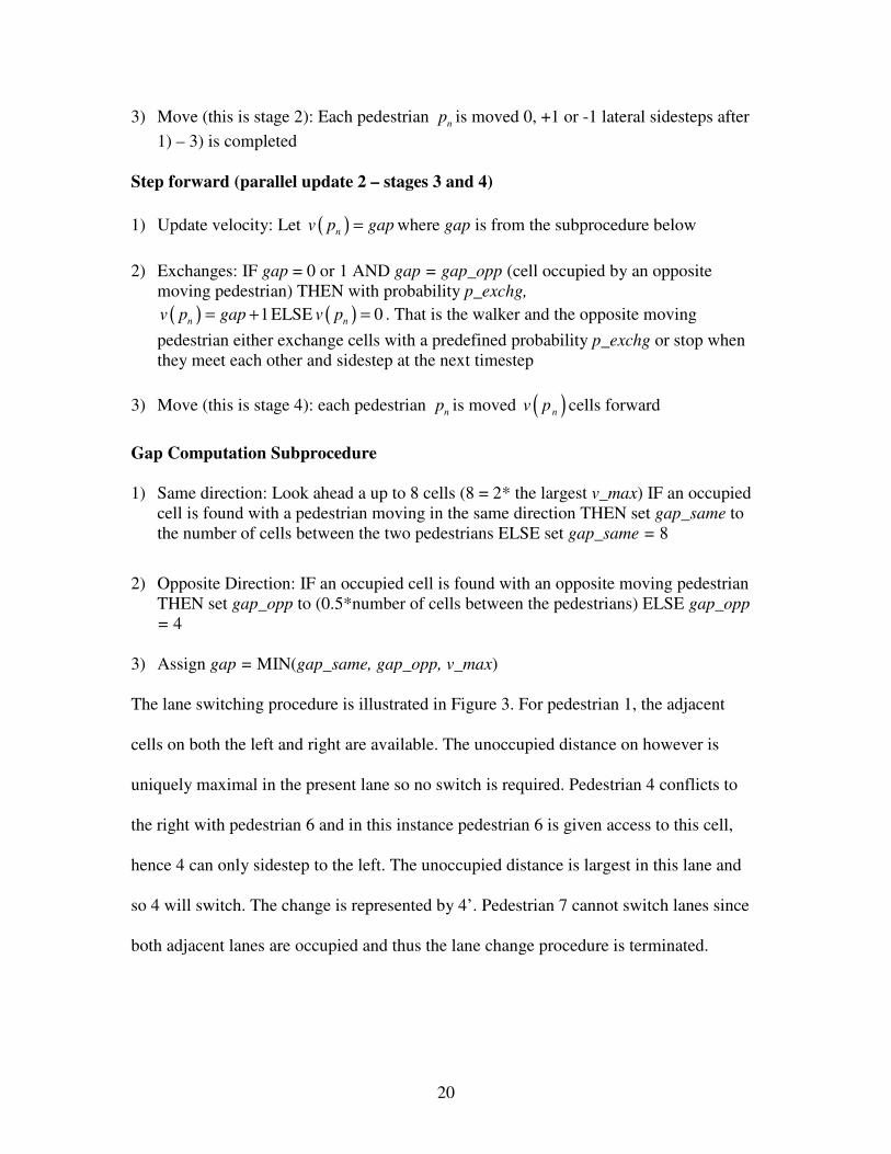
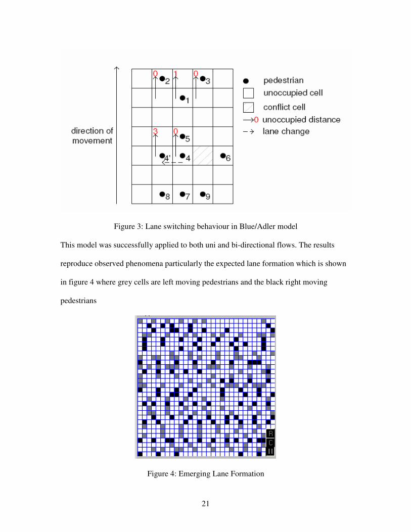
This model was successfully applied to both uni and bi-directional flows. The results
reproduce observed phenomena particularly the expected lane formation which is shown
in figure 4 where grey cells are left moving pedestrians and the black right moving
pedestrians
Figure 4: Emerging Lane Formation
22
Another interesting model was developed by J. Dijkstra, J. Jessurun and H. Timmermans
[10] which looks at pedestrian movement with a shopping centre. The rule set for this
model is
1) Check decision point: If a pedestrian has passed a decision point (the end of an
activity or node in the network) then got 3)
2) Check the cell type – examine the behaviour of the pedestrian and the walkers desired
direction followed by a change into that direction then a decision point will be passed
3) If the cell is free then the pedestrian can move into that cell, otherwise got 4)
4) If the cell to the left/right isn’t occupied then move there
In this model the movement is directed only toward the destination and can only change
at decision points with pedestrian interactions not being considered.
2.6 The Social Force Model
This model has been developed primarily by D. Helbing and P. Molnár ([1], [2], [11]).
They describe the idea of social forces in the context of ordinary pedestrian behaviour.
That is, in general a pedestrian will be used to the majority of situations that confront
them and they have prescribed behavioural strategies based on previous experience of
similar situations. As such they will react in the best way, that is the most efficient for
them and as such pedestrian movement is automatic and thus predictable. The Social
Force Model is a Microsimulation of each individuals behaviour and so each
pedestrian,α , in the system can be represented by a point ( )r tα
� in space, which changes
continuously with speed being governed by the equation of motion
( )
( )dr t
v tdt
αα=
��
(2.6.1)
23
Similarly, the speed ( )v tα
�is continuously changing and thus acceleration is governed by
the social forces ( )f tα
�, which represent the sum of the different influences upon the
individual pedestrian (that is environment and other pedestrians). There is also a
consideration for random fluctuations within the system which account for random
behavioural fluctuations which gives rise to ( )tαξ�
. So, the acceleration obtained is
( ) ( )dv
f t tdt
αα αξ= +
� � � (2.6.2)
The model being implemented in this thesis takes into account an acceleration force
( )0f vα α
� �, repulsive effects of boundaries ( )Bf rα α
� �, repulsive interactions with other
pedestrians ( ), , ,f r v r vαβ α α β β
� � � � � and attraction effects ( ), ,i if r r tα α
� � �leading to
( ) ( ) ( ) ( ) ( )( )
0 , , , , ,B i i
i
f t f v f r f r v r v f r r tα α α α α αβ α α β β α αβ α≠
= + + + � � � � �� � � � � � � �
(2.6.3)
2.6.1 The Driving Force
As the name suggests, the driving force, is the component of the social forces which
describes each individuals desire to move to their intended destination with some desired
velocity 0vα . The desired direction of motion is given by eα
� and deviations of the actual
velocity vα
�from the desired velocity ( ) ( ) ( )0 0
v t v t e tα α α=� �
are corrected within the so
called relaxation time ατ . The equation which describes this motivation is
( ) ( ) ( )( )0 01f v t e t v tα α α α
ατ= −
� � � (2.6.4)
The desired direction of the pedestrian is described by
( )p r
e tp r
αα
α
−=
−
� ��
� � (2.6.5)
24
Where p�
is the desired destination and rα
�the current position.
It is often the case that pedestrians may be delayed, at bottlenecks or doorways for
example, which leads to an increase in the desired speed over the course of time. One
way to describe this effect is to implement the following
( ) ( ) ( ) ( )0 0 max1 0v t n t v n t vα α α α α= − +� �� � (2.6.6)
With, maxvα the maximum desired velocity and ( )0 0vα the initial one. The parameter
( )( )( )0
1v t
n tv t
αα
α
= − (2.6.7)
Describes the impatience of the pedestrian to reach their destination, with ( )v t the
average speed into the desired direction of motion. This particular effect may lead to a
crowd developing pushy behaviour thus increasing the pressure within the crowd, which
may lead to clogging effects which may have disastrous consequences.
2.6.2 Pedestrian Interactions
The repulsive force term ( ), , ,f r v r vαβ α α β β
� � � � �describes the interactions between two
pedestrians and α β , and the desire of pedestrianα to keep a certain distance from β .
This term is described by
( )( ) ( )1 2
1 2exp . exp
r d r df t A n F A n
B B
αβ αβ αβ αβ
αβ α αβ αβ α αβ
α α
� � � �− −= +
� � � �
� � � (2.6.8)
The first term of this force describes the tendency to respect the private sphere of each
individual and also helps to avoid collisions if there are sudden changes within the
system. The second term accounts for the behaviour of physical interaction in high
25
densities and pushy crowds if so called frictional effects are ignored. A second
formulation which includes frictional effects will be briefly introduced later. The
parameters and i iA Bα α denote the interaction strength and range respectively. These
parameters are often dependent on cultural influences, for example the personal space
expected may vary depending on the society being modelled. The parameter dαβ is the
distance between the centres of mass of the pedestrians being considered, rαβ is the sum
of the radii of pedestrians and α β and nαβ
�is the normalised vector pointing from to β α
( ) ( )
( )x t x t
nd t
α βαβ
αβ
−=
� ��
(2.6.9)
Where ( )x tα
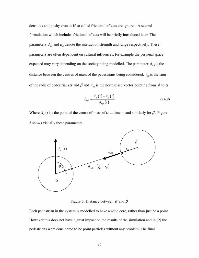
�is the point of the centre of mass of at time tα , and similarly for β . Figure
5 shows visually these parameters.
Figure 5: Distance between and α β
Each pedestrian in the system is modelled to have a solid core, rather than just be a point.
However this does not have a great impact on the results of the simulation and in [2] the
pedestrians were considered to be point particles without any problem. The final
α
β
( )d r rαβ α β− +
rα
rβ nαβ
�
( )e tα
�
αβϕ
26
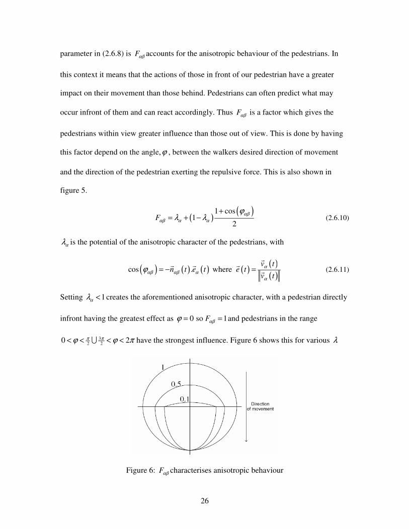
parameter in (2.6.8) is Fαβ accounts for the anisotropic behaviour of the pedestrians. In
this context it means that the actions of those in front of our pedestrian have a greater
impact on their movement than those behind. Pedestrians can often predict what may
occur infront of them and can react accordingly. Thus Fαβ is a factor which gives the
pedestrians within view greater influence than those out of view. This is done by having
this factor depend on the angle,ϕ , between the walkers desired direction of movement
and the direction of the pedestrian exerting the repulsive force. This is also shown in
figure 5.
( )( )1 cos
12
Fαβ
αβ α α
ϕλ λ
+= + − (2.6.10)
αλ is the potential of the anisotropic character of the pedestrians, with
( ) ( ) ( ) ( )( )( )
cos . where v t
n t e t e tv t
ααβ αβ α
α
ϕ = − =
�� � �
� (2.6.11)
Setting 1αλ < creates the aforementioned anisotropic character, with a pedestrian directly
infront having the greatest effect as 0 so 1Fαβϕ = = and pedestrians in the range
32 2
0 2π πϕ ϕ π< < < <� have the strongest influence. Figure 6 shows this for various λ
Figure 6: Fαβ characterises anisotropic behaviour
27
2.6.3 Boundary Interactions
The treatment of boundaries within the model is analogous to that of other pedestrians,
excluding the anisotropic effects of the pedestrian interactions. This leads to
( ) exp BB B
B
r df r A n
B
α αα α α α
α
Β
� �−= � �
� �
� � � (2.6.12)
Where B
dα is the distance between the boundary and the pedestrian and B
nα
�the normal
vector pointing from the boundary toα . In most situations there is more than one
boundary to consider leading to a question as to which boundaries influence to account
for. There are three possible ways of considering the boundary interaction
1. Superposition: All boundaries influence the pedestrian so the forces are summed
2. Shortest distance: Only the closet boundary element is considered
3. Biggest impact: only the boundary with the largest impact is considered
In most geometries the biggest impact and shortest distance model are equivalent; this is
often an appropriate choice too however this may not however be reasonable for angled
passageways and superposition may be better. It was decided that in this project only the
nearest boundary element would be considered, again this was the approach of [2] and
produced realistic results in that case.
2.6.4 Attractive Interactions
Often pedestrians demonstrate certain joining characteristics, such as families or groups
of tourists, and will wish to move through the walkway together. Other instances may be
shops, window displays or performances in the street. These two cases are however
separate, in the former the attractive force is constant and independent of time reflecting
the desire of these groups to remain together over the whole time interval. In the latter
28
case however the attraction is time dependent as the pedestrian will not wish to be late
and clearly will ignore the attraction if this is the case. Such attractions have a similar
modelling to pedestrian interactions however the attraction range i
Bα is typically larger
with a smaller, negative, time dependent interaction strengthi
Aα .
2.6.5 Individuality and Random Behaviour Fluctuations
As previously mentioned, each pedestrian may display some random behaviour arising
from accidental or deliberate changes to the expected and optimal actions. This force
( )tαξ�
is Gaussian distributed and perpendicular to the desired direction. One such
formulation would be
( ) ( ) perp,e t f t Xeα α α αξ =�� �
(2.6.13)
Here ( )20,X N σ∝ with probability density
( )2
2
1 1. exp
22
xf x
σ σπ
� �−= � �
� � (2.6.14)
2.6.6 Another Formulation
As previously mentioned, there is another formulation of the Social Force model which
takes into account the ‘sliding friction force’ in the pedestrian and boundary interaction
terms. For the pedestrian interactions the model becomes
( ) ( )exp . . . tr d
f A F k g r d n g r d v tB
αβ αβαβ α αβ αβ αβ αβ αβ αβ αβ αβ
α
κ� �−� �� �
= + − + − ∆� �� �� �� �� �
� ��(2.6.15)
Here ( )2 1,t n nαβ αβ αβ= −�
is the tangential direction and ( ).tv v v tαβ β α αβ∆ = −�� �
the relative
tangential velocity. The values , k κ are given constants of the system and the function
29
( )g x is zero when its argument is negative and equal to its argument otherwise. In this
case
( )0 if
else
d rg r d
r d
αβ αβ
αβ αβ
αβ αβ
>��− = �
−�� (2.6.16)
Physically this means that the ‘sliding friction force’ is only felt if the pedestrians are
touching. Again boundary interactions are analogous, so
( ) ( )( )exp . . .BB B B B B B gaB
B
r df A k g r d n g r d v t t
B
α αα α α α α α α α α
α
κ� �� �−� �
= + − − −� �� �� �� �� �
� � �� � (2.6.17)
This alternative model will not be implemented (although in principle once the first
model is coded the changes required are not difficult) and is only included for
completeness. Similarly the attractive interactions and random fluctuations described
earlier will not be implemented either.
30
Chapter 3
Self-Organisation Phenomena in Pedestrian Flows
One of the main objectives of this thesis is to explore and simulate emergent behaviours
of pedestrian systems. If a pedestrian flow has certain conditions such phenomena are
often observable. Of particular interest are
• Lane formation and striping effects
• Oscillatory flows and clogging effects at doorways
• Shock waves in dense crowds
These self-organisation effects are patterns of behaviour that are not externally planned or
organised by an outside source such as traffic signals or behavioural conventions.
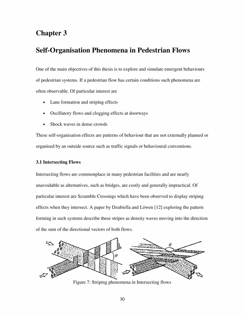
3.1 Intersecting Flows
Intersecting flows are commonplace in many pedestrian facilities and are nearly
unavoidable as alternatives, such as bridges, are costly and generally impractical. Of
particular interest are Scramble Crossings which have been observed to display striping
effects when they intersect. A paper by Dzubiella and Löwen [12] exploring the pattern
forming in such systems describe these stripes as density waves moving into the direction
of the sum of the directional vectors of both flows.
Figure 7: Striping phenomena in Intersecting flows
θ
θ
31
The stripe formation reduces the number of obstructing interactions and maximisation of
average pedestrian speeds.
3.2 Bottlenecks
Bottlenecks such as doorways are also common in pedestrian areas and the way
pedestrians interact at them is of interest. Often the flows through bottlenecks are
irregular and inefficient. If there is an opposite flow into a bottleneck it is often the case
that the flow of pedestrians is oscillating and unidirectional as opposed to the
bidirectional flow in an ordinary corridor without a bottleneck. Similar to lane formation,
which will be discussed in the next section, it is typical for groups to move through the
bottle neck since it is easier to follow someone than to move against them. This leads to a
pressure increase, due in part to impatience, on the side of the bottleneck where flow is
halted and a decrease on the side that is flowing. When the difference between the two
pressures is large enough the flow will change. Thus the process is reversed and the flows
will oscillate.
3.3 Lane Formation
A bidirectional system, or counterflow, in everyday conditions has pedestrians moving in
opposite directions which are unevenly distributed over the walkway. One of the most
commonly observed phenomena is lane formation where pedestrians form into lanes of
unidirectional flow. This effect leads to a reduction in the number of evasive manoeuvres
each pedestrian need to make and so increases the efficiency of the walkway. In this case,
improved efficiency means that the average pedestrian speed is maximal and necessary
avoidance and braking actions minimal. The number of lanes formed is dependent on the
32
geometry of the walkway. Initially the lanes are small channels, created when opposite
moving pedestrians meet, which then merge with each other to form larger lanes.
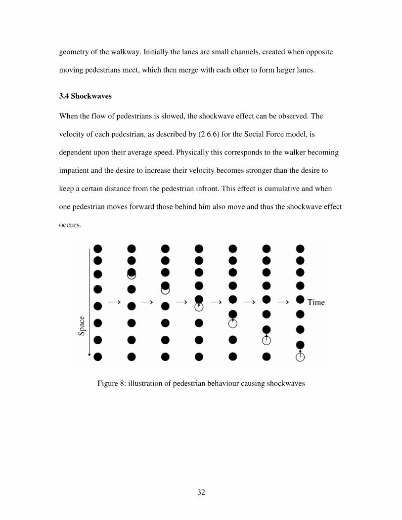
3.4 Shockwaves
When the flow of pedestrians is slowed, the shockwave effect can be observed. The
velocity of each pedestrian, as described by (2.6.6) for the Social Force model, is
dependent upon their average speed. Physically this corresponds to the walker becoming
impatient and the desire to increase their velocity becomes stronger than the desire to
keep a certain distance from the pedestrian infront. This effect is cumulative and when
one pedestrian moves forward those behind him also move and thus the shockwave effect
occurs.
Figure 8: illustration of pedestrian behaviour causing shockwaves
33
Chapter 4
Implementation of the Social Force Model
One of the key aims of this project was to successfully implement the Social Force
Model, as described by Helbing [1], and attempt to do some quantitative analysis of the
results along with reproducing the qualitative behaviours of large pedestrian flows as
described in chapter 3. In this chapter the implementation of this model will be explored
with particular emphasis given to detailing some of the problems observed with the
model and how they were overcome.
4.1 Numerical Solution of the Social Force Model
The Social Force Model described in chapter 2 is a first order Ordinary Differential
Equation (ODE) which needs to be solved numerically to calculate the velocity and
position of the pedestrians within the system. Importantly the model is an initial value
problem, for both the velocity and displacement equations, which means that there are
several excellent MATLAB solvers available for this type of problem. The ODE
described by the Social Force model with initial conditions
( ) ( ) ( )( )
( ) ( ) ( )( )
1 2
1 2
0 0 , 0
0 0 , 0
t
t
r r r
v v v
α α α
α α α
=
=
�
� (4.1.1)
Is a non-stiff system, as all the elements evolve on a similar time-scale. As this is the case
the suggested solver initially was ode45 which is extremely efficient for these types of
problem. This solver implements a Runge Kutta method of the fourth order and was
developed by Dormand and Prince. However, an unspotted error in the initial code
34
actually meant that it appeared that the system was stiff and so a different solver was
chosen, namely ode15s which is a Gear solver and generally very efficient for stiff
systems. This error was subsequently spotted in the de-bugging procedure and obviously
raised the question as to whether ode15s was an appropriate solver for the system. To
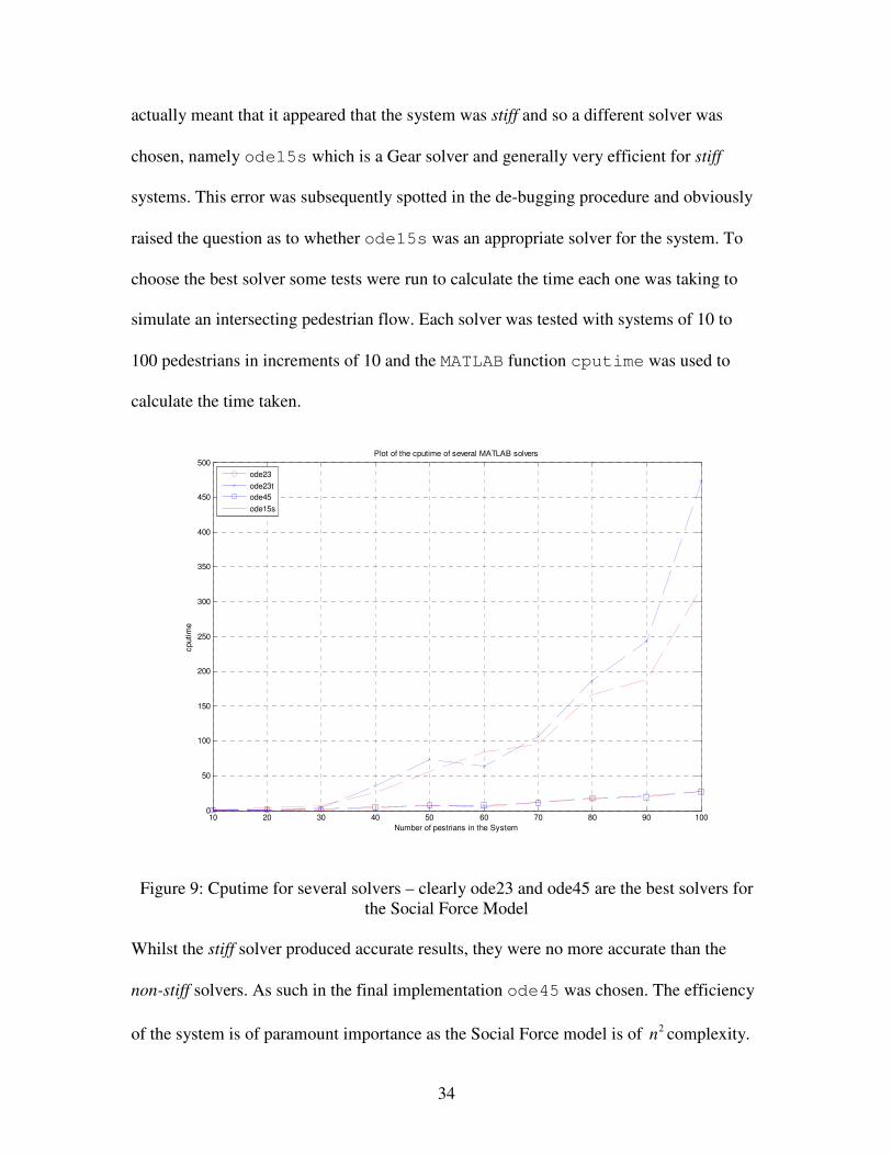
choose the best solver some tests were run to calculate the time each one was taking to
simulate an intersecting pedestrian flow. Each solver was tested with systems of 10 to
100 pedestrians in increments of 10 and the MATLAB function cputime was used to
calculate the time taken.
10 20 30 40 50 60 70 80 90 1000
50
100
150
200
250
300
350
400
450
500
Number of pestrians in the System
cputim
e
Plot of the cputime of several MATLAB solvers
ode23
ode23t
ode45
ode15s
Figure 9: Cputime for several solvers – clearly ode23 and ode45 are the best solvers for
the Social Force Model
Whilst the stiff solver produced accurate results, they were no more accurate than the
non-stiff solvers. As such in the final implementation ode45 was chosen. The efficiency
of the system is of paramount importance as the Social Force model is of 2n complexity.
35
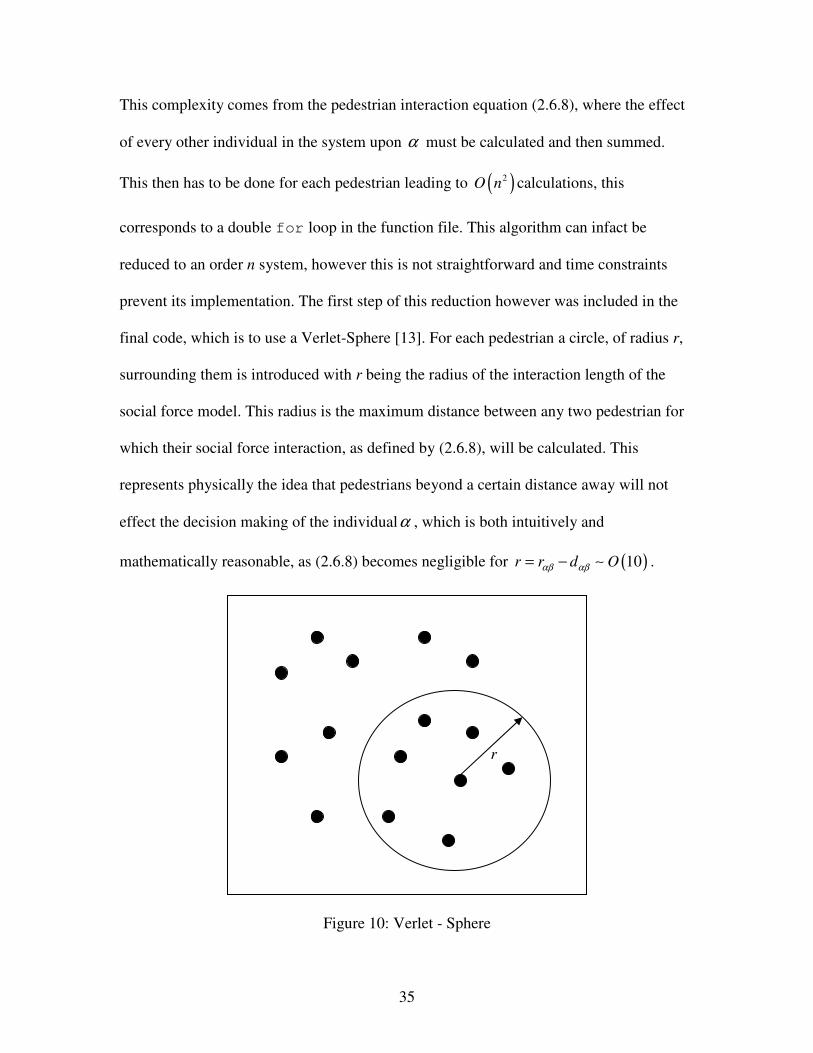
This complexity comes from the pedestrian interaction equation (2.6.8), where the effect
of every other individual in the system upon α must be calculated and then summed.
This then has to be done for each pedestrian leading to ( )2O n calculations, this
corresponds to a double for loop in the function file. This algorithm can infact be
reduced to an order n system, however this is not straightforward and time constraints
prevent its implementation. The first step of this reduction however was included in the
final code, which is to use a Verlet-Sphere [13]. For each pedestrian a circle, of radius r,
surrounding them is introduced with r being the radius of the interaction length of the
social force model. This radius is the maximum distance between any two pedestrian for
which their social force interaction, as defined by (2.6.8), will be calculated. This
represents physically the idea that pedestrians beyond a certain distance away will not
effect the decision making of the individualα , which is both intuitively and
mathematically reasonable, as (2.6.8) becomes negligible for ( )10r r d Oαβ αβ= − � .
Figure 10: Verlet - Sphere
r
36
The final code for the simulation solves 4n differential equations, where n is the number
of pedestrians in the system. To solve, ode15s requires a vector input with each
component corresponding to a differential equation. The first 2n differential equations are
the x and y velocity components for pedestrians 1 to n and the second 2n differential
equations the x and y displacement values for pedestrians 1 to n. That is
( )
( )
( )
( )
1 1
2 2 for 1,...,
v t f tdn
dt v t f t
α α
α α
α� � � �
= = � � � �
(4.1.2)
and
( )
( )
( )
( )
1 1
2 2 for 1,...,
r t v tdn
dt r t v t
α α
α α
α� � � �
= = � � � �
(4.1.3)
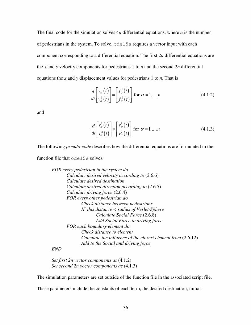
The following pseudo-code describes how the differential equations are formulated in the
function file that ode15s solves.
FOR every pedestrian in the system do
Calculate desired velocity according to (2.6.6)
Calculate desired destination
Calculate desired direction according to (2.6.5)
Calculate driving force (2.6.4)
FOR every other pedestrian do
Check distance between pedestrians
IF this distance < radius of Verlet-Sphere
Calculate Social Force (2.6.8)
Add Social Force to driving force
FOR each boundary element do
Check distance to element
Calculate the influence of the closest element from (2.6.12)
Add to the Social and driving force
END
Set first 2n vector components as (4.1.2)
Set second 2n vector components as (4.1.3)
The simulation parameters are set outside of the function file in the associated script file.
These parameters include the constants of each term, the desired destination, initial
37
position and velocities and the boundary array which describes the geometry of the room
being considered.
4.2 The Desired Destination and Waypoints
In the earlier version of the code, the desired destination was set as a single point which
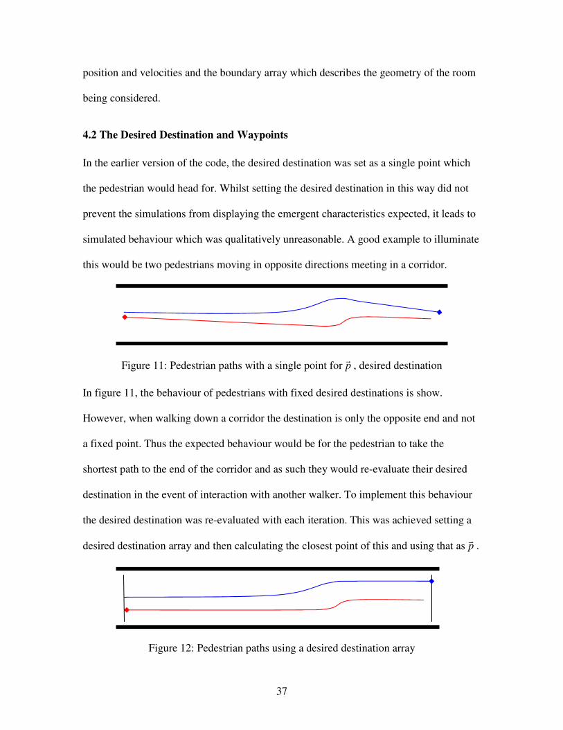
the pedestrian would head for. Whilst setting the desired destination in this way did not
prevent the simulations from displaying the emergent characteristics expected, it leads to
simulated behaviour which was qualitatively unreasonable. A good example to illuminate
this would be two pedestrians moving in opposite directions meeting in a corridor.
Figure 11: Pedestrian paths with a single point for p�
, desired destination
In figure 11, the behaviour of pedestrians with fixed desired destinations is show.
However, when walking down a corridor the destination is only the opposite end and not
a fixed point. Thus the expected behaviour would be for the pedestrian to take the
shortest path to the end of the corridor and as such they would re-evaluate their desired
destination in the event of interaction with another walker. To implement this behaviour
the desired destination was re-evaluated with each iteration. This was achieved setting a
desired destination array and then calculating the closest point of this and using that as p�
.
Figure 12: Pedestrian paths using a desired destination array
38
In Figure 12 the desired destination arrays are shown at each end of the corridor and the
new pedestrian paths. In this small test case the difference may seem to be unimportant
but its value in the modelling come as the number of pedestrians in the system increase. If
the desired destination remained as a single point then individuals maybe simulated
trying to force their way through a dense crowd to reach the specified point instead of
taking the more efficient route. The principle at the core of all pedestrian modelling is
that individuals will try to use the most efficient route for themselves and that the model
must reflect the decision making abilities of humans and their capability to change and
adapt to the system around them.
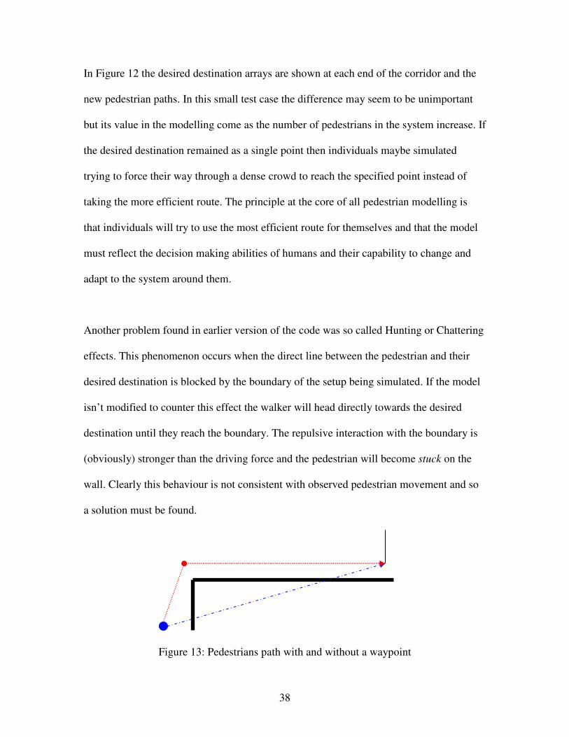
Another problem found in earlier version of the code was so called Hunting or Chattering
effects. This phenomenon occurs when the direct line between the pedestrian and their
desired destination is blocked by the boundary of the setup being simulated. If the model
isn’t modified to counter this effect the walker will head directly towards the desired
destination until they reach the boundary. The repulsive interaction with the boundary is
(obviously) stronger than the driving force and the pedestrian will become stuck on the
wall. Clearly this behaviour is not consistent with observed pedestrian movement and so
a solution must be found.
Figure 13: Pedestrians path with and without a waypoint
39
The solution implement in here is to use a waypoint system. In Figure 13 the blue dashed
line illustrates the desired path of the pedestrian in the original code and the red line the
desired path after a waypoint is included. The process of implementing waypoints is
relatively straight forward, the pseudo-code is as follows:
FOR each pedestrian do
Check the distance from current position to waypoint (i)
IF the distance to waypoint (i) < specified distance
Set desired destination as the waypoint (i + 1)
ELSE
Set desired destination as waypoint (i)
END
END
Again it is important to note that waypoints are intuitively consistent with pedestrian
behaviour, in particular a pedestrians immediate destination is always within their line of
sight. That is, an individual will always travel to a place they can see until their ultimate
destination is in view. In the case of angled passage ways, corners will be appropriate
waypoints since moving directly toward them will provide the shortest path to the overall
goal.
4.3 The Desired Velocity
One of the self-organisation phenomena of interest are shockwaves in dense crowds. This
effect comes from an impatience factor of the modelled pedestrians. This is described in
the formulation of the desired velocity, (2.6.6). The only extra calculation required is the
average velocity, which is
( ) ( )0r t r
vt
α αα
−=
� �
(4.3.1)
40
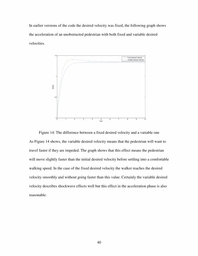
In earlier versions of the code the desired velocity was fixed, the following graph shows
the acceleration of an unobstructed pedestrian with both fixed and variable desired
velocities.
0 1 2 3 4 5 6 7 8 9 100
0.5
1
1.5
Time
Speed
Fixed Desired Velocity
Variable Desired Velocity
Figure 14: The difference between a fixed desired velocity and a variable one
As Figure 14 shows, the variable desired velocity means that the pedestrian will want to
travel faster if they are impeded. The graph shows that this effect means the pedestrian
will move slightly faster than the initial desired velocity before settling into a comfortable
walking speed. In the case of the fixed desired velocity the walker reaches the desired
velocity smoothly and without going faster than this value. Certainly the variable desired
velocity describes shockwave effects well but this effect in the acceleration phase is also
reasonable.
41
Chapter 5
Simulation and Analysis of the Social Force Model
In this chapter the code created to implement the Social Force Model will be run for a
variety of different pedestrian flows. These will be a counterflow within a corridor, with
and without a bottleneck, a ninety degree corner and finally a Scramble Crossing. The
aim will be to use the data from the simulation to do some quantitative analysis of
pedestrian flows to supplement the qualitative observations laid out in chapter 3.
Obviously it is expected that the model will recreate self organisation phenomena and
where this is the case it will be highlighted.
5.1 The Model Constants
The Social Force Model has several parameters in each of the driving force (2.6.4),
pedestrian interaction (2.6.8), and boundary interaction terms (2.6.12). Thus, several
parameters must be set in the startup phase of the simulation, in this instance in the script
file for the model.
The driving force parameters are consistent with those of Helbing [1] where the desired
velocity is set to 1.34 ms-1
with a relaxation time, ατ , of 0.5. The relaxation time is the
time taken to correct disturbance in movement (e.g. obstacles or avoidance manoeuvres).
Helbing also gives values for the parameters in the pedestrian and boundary interaction
terms. To verify that these values were reasonable the simulation was run for a variety of
parameters in a test room and the resulting pedestrian flows evaluated.
42
0 2 4 6 8 10 12 14 16 18 200
1
2
3
4
5
6
7
8
9
10
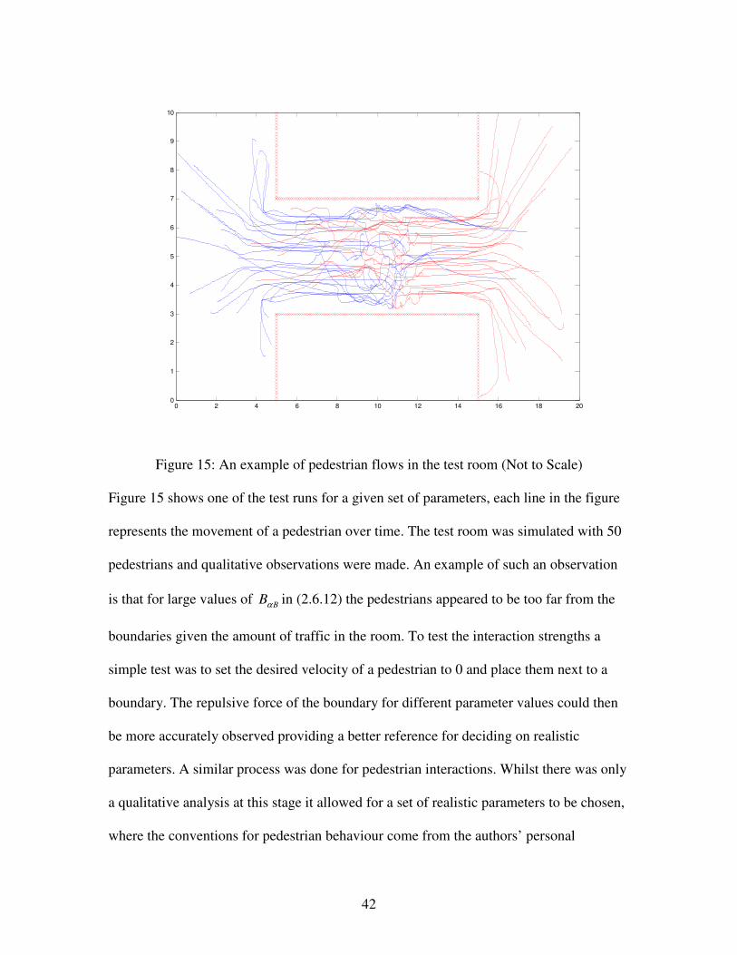
Figure 15: An example of pedestrian flows in the test room (Not to Scale)
Figure 15 shows one of the test runs for a given set of parameters, each line in the figure
represents the movement of a pedestrian over time. The test room was simulated with 50
pedestrians and qualitative observations were made. An example of such an observation
is that for large values of B
Bα in (2.6.12) the pedestrians appeared to be too far from the
boundaries given the amount of traffic in the room. To test the interaction strengths a
simple test was to set the desired velocity of a pedestrian to 0 and place them next to a
boundary. The repulsive force of the boundary for different parameter values could then
be more accurately observed providing a better reference for deciding on realistic
parameters. A similar process was done for pedestrian interactions. Whilst there was only
a qualitative analysis at this stage it allowed for a set of realistic parameters to be chosen,
where the conventions for pedestrian behaviour come from the authors’ personal
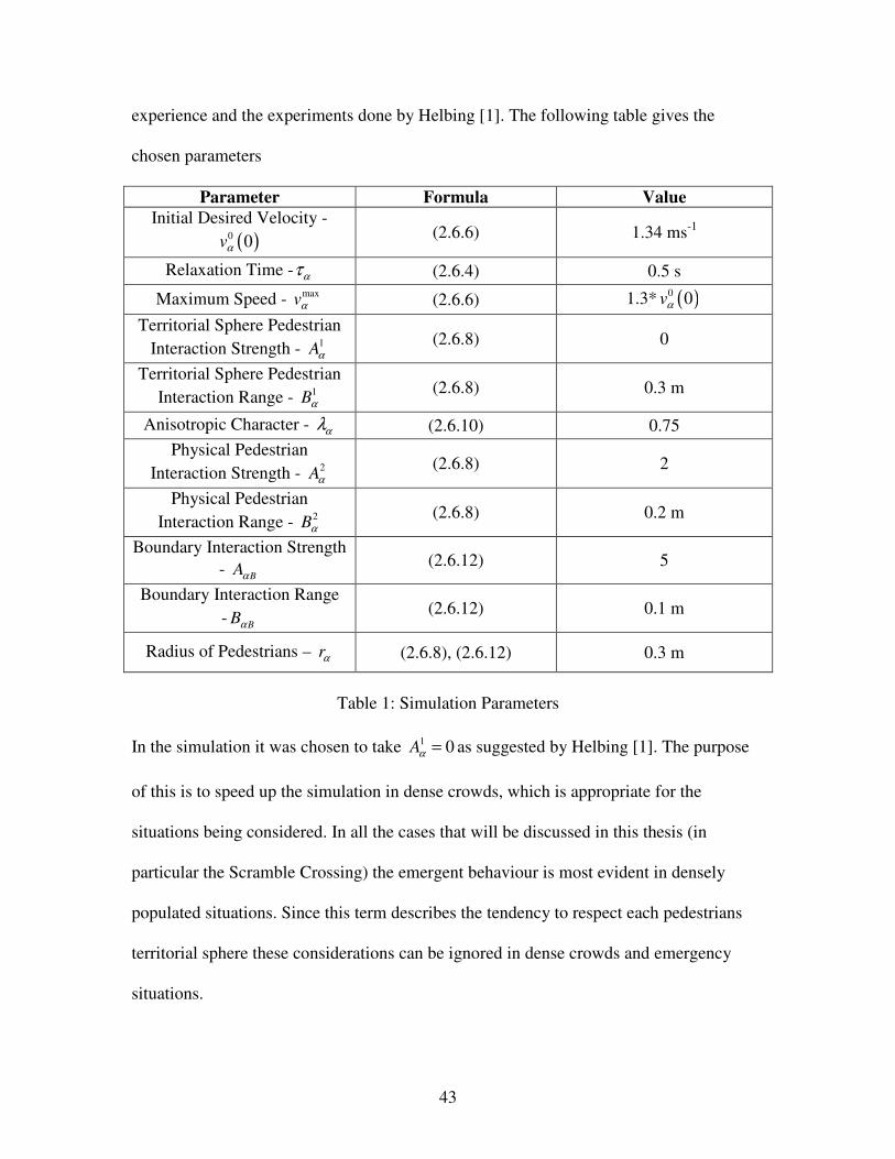
43
experience and the experiments done by Helbing [1]. The following table gives the
chosen parameters
Parameter Formula Value
Initial Desired Velocity -
( )0 0vα (2.6.6) 1.34 ms
-1
Relaxation Time - ατ (2.6.4) 0.5 s
Maximum Speed - maxvα (2.6.6) 1.3* ( )0 0vα
Territorial Sphere Pedestrian
Interaction Strength - 1Aα
(2.6.8) 0
Territorial Sphere Pedestrian
Interaction Range - 1Bα
(2.6.8) 0.3 m
Anisotropic Character - αλ (2.6.10) 0.75
Physical Pedestrian
Interaction Strength - 2Aα
(2.6.8) 2
Physical Pedestrian
Interaction Range - 2Bα
(2.6.8) 0.2 m
Boundary Interaction Strength
- B
Aα (2.6.12) 5
Boundary Interaction Range
-B
Bα (2.6.12) 0.1 m
Radius of Pedestrians – rα (2.6.8), (2.6.12) 0.3 m
Table 1: Simulation Parameters
In the simulation it was chosen to take 1 0Aα = as suggested by Helbing [1]. The purpose
of this is to speed up the simulation in dense crowds, which is appropriate for the
situations being considered. In all the cases that will be discussed in this thesis (in
particular the Scramble Crossing) the emergent behaviour is most evident in densely
populated situations. Since this term describes the tendency to respect each pedestrians
territorial sphere these considerations can be ignored in dense crowds and emergency
situations.
44
One final consideration in the startup phase is the size of the so-called Verlet-Sphere
implemented in (2.6.8) discussed in chapter 4. The radius was chosen to be 10 m,
anything further away than this has an overall contribution to the social force felt byα to
be ( )1510O −≥ which is negligible since the cumulative social force of all pedestrians
uponα is of ( )1O .
5.2 Pedestrian Counterflows
In this section the code developed will be used to simulate pedestrian counterflows both
with and without a bottleneck in the walkway. The purpose of modelling these situations
is to assess the validity of the simulation in a qualitative sense. In chapter 3 certain
emergent phenomena were discussed; in particular lane formation in a counterflow and
oscillatory flow at bottleneck. For these particular geometries a more detailed analysis of
the pedestrian movements will not be considered, rather this section aims to confirm that
the model simulates well experimentally observed phenomena ([1], [2]).
In a counterflow expected emergent behaviour is lane formation as discussed in chapter
3. The simulation was run for 250 pedestrians on a 200 meter walkway which is 6 meters
wide. Half the pedestrians were randomly placed at each end of the walkway with a
bivariate uniform distribution using the rand function in MATLAB. The wavefront of
each the pedestrian bodies (in this case the group at either end) meet at the middle of the
walkway. The simulation results were used to produce a movie (submitted on cd with the
thesis – the file ‘250conterflow.avi’) of the pedestrian movement.
45
25 30 35 40 45 50 55 60 65 70 750
2
4
6
8
10
12
14
16
18
20
25 30 35 40 45 50 55 60 65 70 750
2
4
6
8
10
12
14
16
18
20
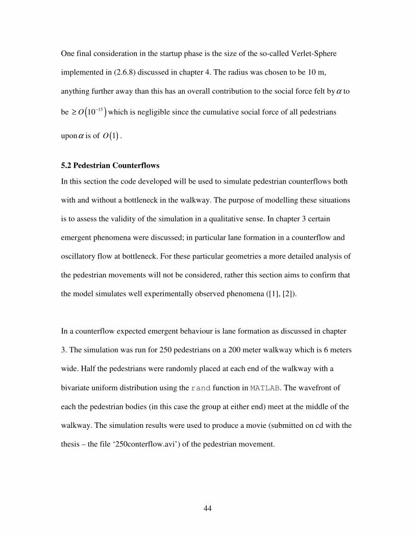
(a) The initial pedestrian distribution (b) The final pedestrian distribution
Figure 16: The initial and final pedestrian positions created for a counterflow
The results of the simulation are better than expected, reproducing the self organisation
phenomena perfectly. However these results underline the idealised nature of the
implemented model. In a real counterflow the pedestrians would not be homogeneous,
that is the desired speed of the walkers would not be uniform and the pedestrians radii
would not be the same. These inhomogeneities would lead to behaviour that isn’t
observed in this simulation, a particular example of this would be overtaking manoeuvres
performed by faster moving pedestrians. In walkways with large pedestrian densities
these manoeuvres can lead to a breakdown in the lane formation; this suggests that these
idealisations may not always be valid assumptions.
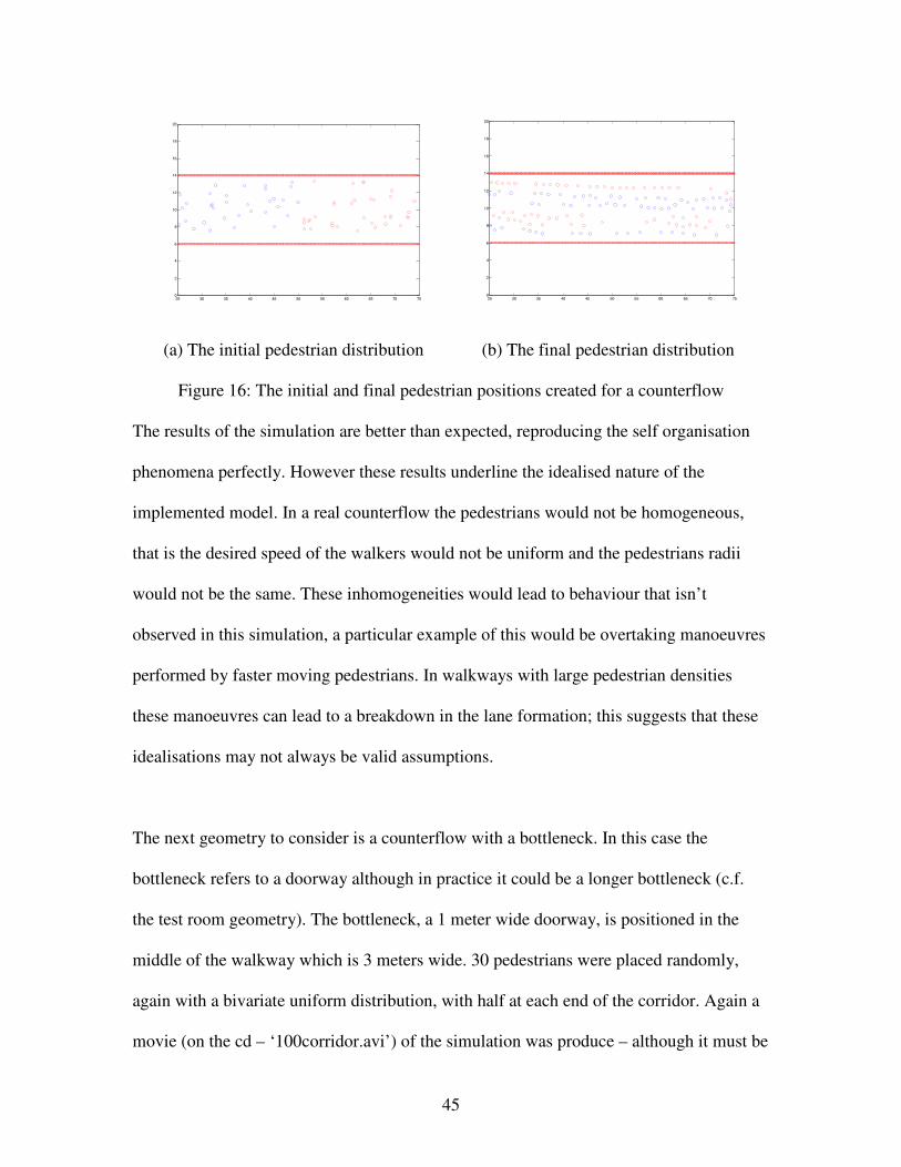
The next geometry to consider is a counterflow with a bottleneck. In this case the
bottleneck refers to a doorway although in practice it could be a longer bottleneck (c.f.
the test room geometry). The bottleneck, a 1 meter wide doorway, is positioned in the
middle of the walkway which is 3 meters wide. 30 pedestrians were placed randomly,
again with a bivariate uniform distribution, with half at each end of the corridor. Again a
movie (on the cd – ‘100corridor.avi’) of the simulation was produce – although it must be
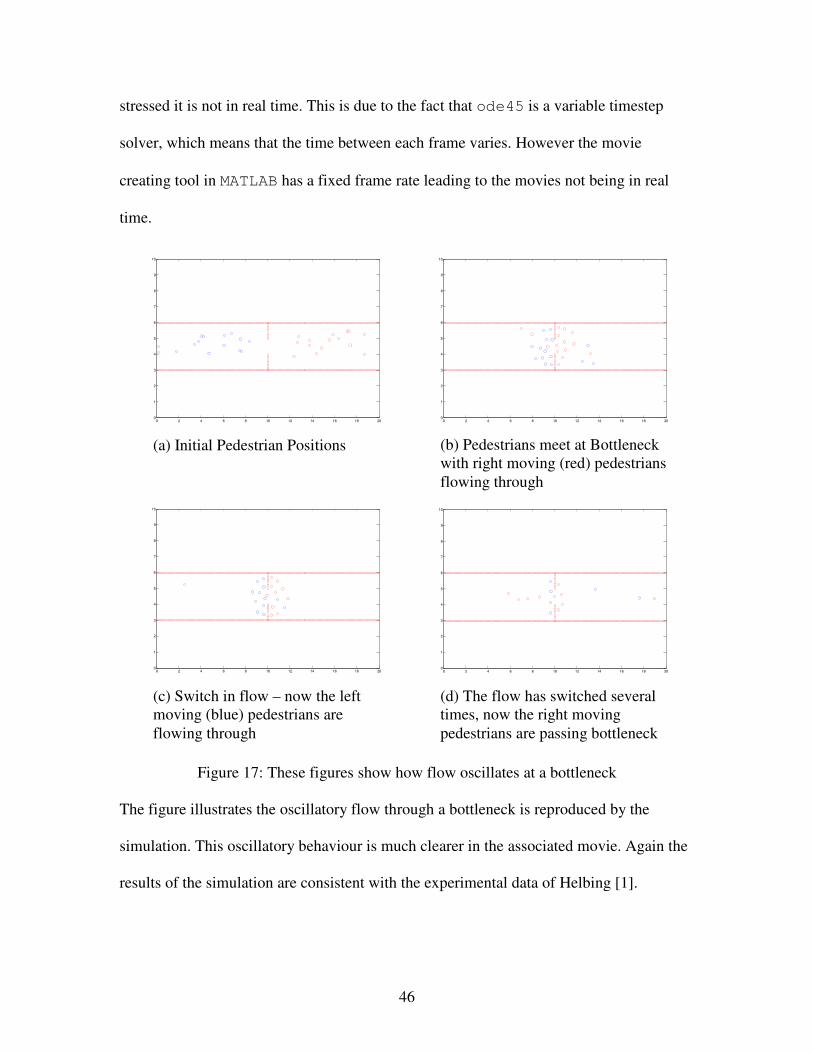
46
stressed it is not in real time. This is due to the fact that ode45 is a variable timestep
solver, which means that the time between each frame varies. However the movie
creating tool in MATLAB has a fixed frame rate leading to the movies not being in real
time.
0 2 4 6 8 10 12 14 16 18 200
1
2
3
4
5
6
7
8
9
10
0 2 4 6 8 10 12 14 16 18 200
1
2
3
4
5
6
7
8
9
10
0 2 4 6 8 10 12 14 16 18 200
1
2
3
4
5
6
7
8
9
10
0 2 4 6 8 10 12 14 16 18 200
1
2
3
4
5
6
7
8
9
10
Figure 17: These figures show how flow oscillates at a bottleneck
The figure illustrates the oscillatory flow through a bottleneck is reproduced by the
simulation. This oscillatory behaviour is much clearer in the associated movie. Again the
results of the simulation are consistent with the experimental data of Helbing [1].
(a) Initial Pedestrian Positions (b) Pedestrians meet at Bottleneck
with right moving (red) pedestrians
flowing through
(c) Switch in flow – now the left
moving (blue) pedestrians are
flowing through
(d) The flow has switched several
times, now the right moving
pedestrians are passing bottleneck
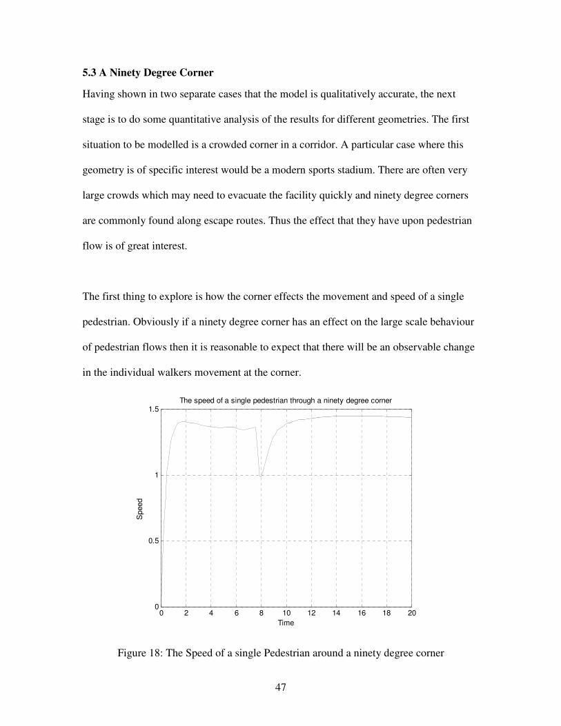
47
5.3 A Ninety Degree Corner
Having shown in two separate cases that the model is qualitatively accurate, the next
stage is to do some quantitative analysis of the results for different geometries. The first
situation to be modelled is a crowded corner in a corridor. A particular case where this
geometry is of specific interest would be a modern sports stadium. There are often very
large crowds which may need to evacuate the facility quickly and ninety degree corners
are commonly found along escape routes. Thus the effect that they have upon pedestrian
flow is of great interest.
The first thing to explore is how the corner effects the movement and speed of a single
pedestrian. Obviously if a ninety degree corner has an effect on the large scale behaviour
of pedestrian flows then it is reasonable to expect that there will be an observable change
in the individual walkers movement at the corner.
0 2 4 6 8 10 12 14 16 18 200
0.5
1
1.5
Time
Speed
The speed of a single pedestrian through a ninety degree corner
Figure 18: The Speed of a single Pedestrian around a ninety degree corner
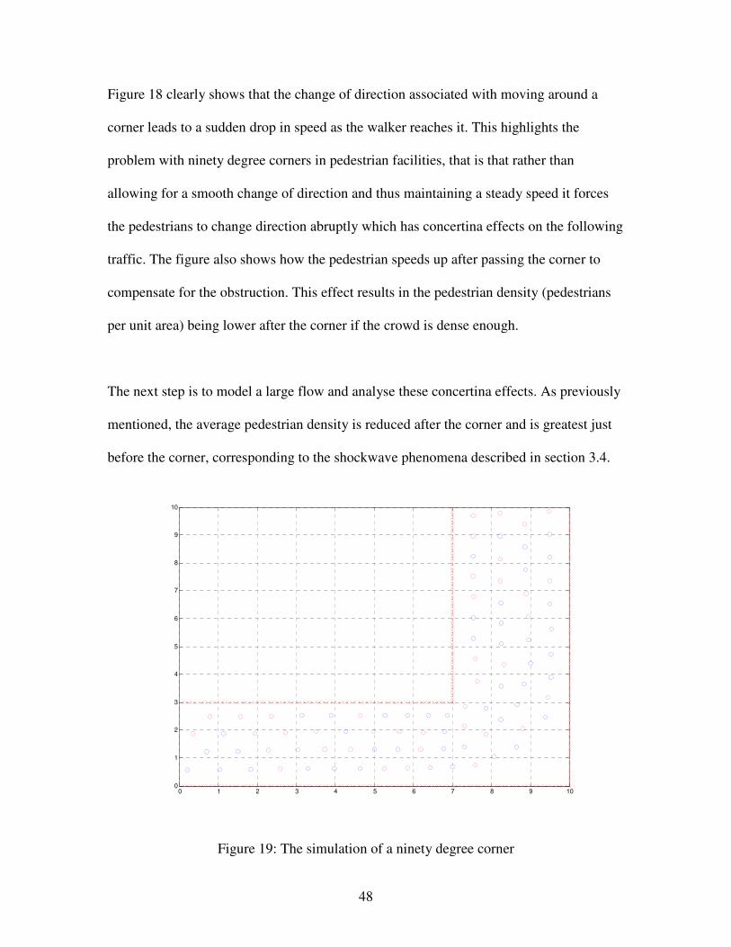
48
Figure 18 clearly shows that the change of direction associated with moving around a
corner leads to a sudden drop in speed as the walker reaches it. This highlights the
problem with ninety degree corners in pedestrian facilities, that is that rather than
allowing for a smooth change of direction and thus maintaining a steady speed it forces
the pedestrians to change direction abruptly which has concertina effects on the following
traffic. The figure also shows how the pedestrian speeds up after passing the corner to
compensate for the obstruction. This effect results in the pedestrian density (pedestrians
per unit area) being lower after the corner if the crowd is dense enough.
The next step is to model a large flow and analyse these concertina effects. As previously
mentioned, the average pedestrian density is reduced after the corner and is greatest just
before the corner, corresponding to the shockwave phenomena described in section 3.4.
0 1 2 3 4 5 6 7 8 9 100
1
2
3
4
5
6
7
8
9
10
Figure 19: The simulation of a ninety degree corner
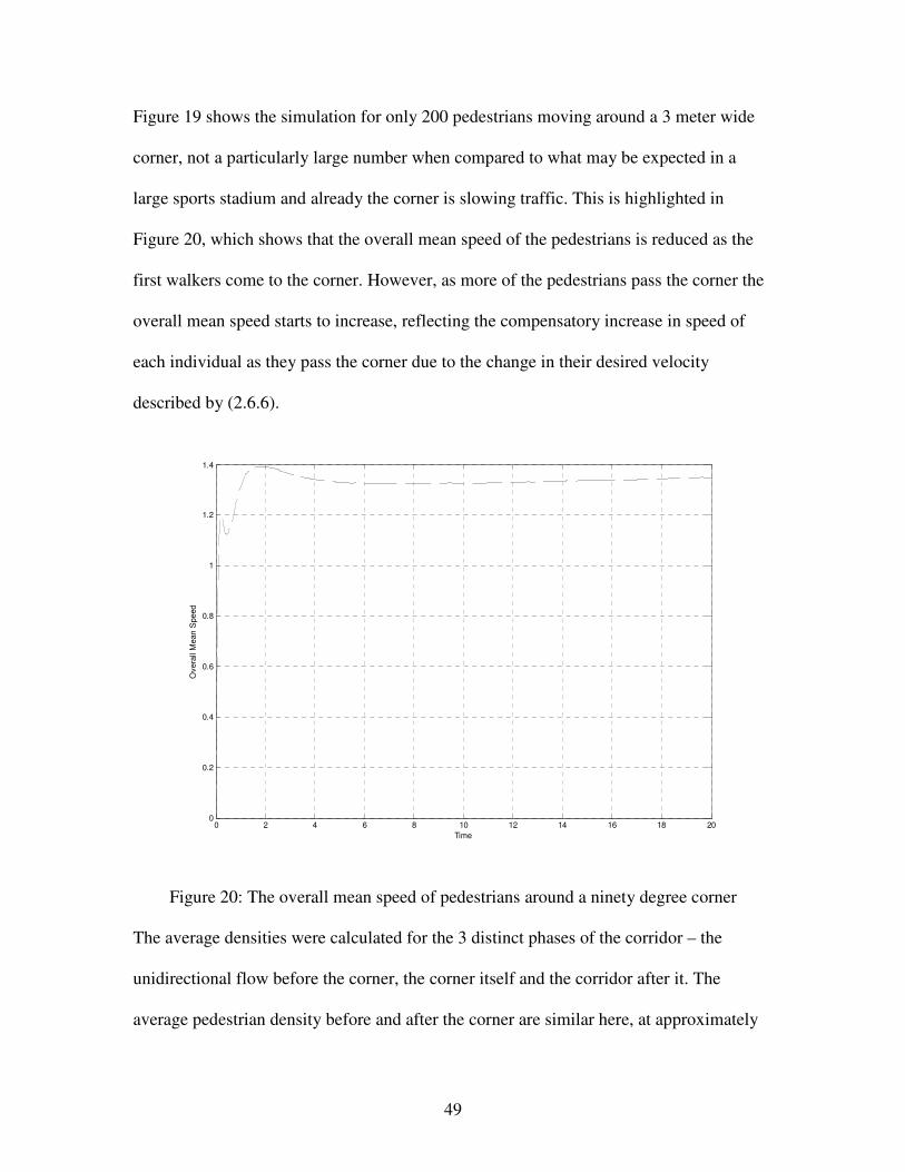
49
Figure 19 shows the simulation for only 200 pedestrians moving around a 3 meter wide
corner, not a particularly large number when compared to what may be expected in a
large sports stadium and already the corner is slowing traffic. This is highlighted in
Figure 20, which shows that the overall mean speed of the pedestrians is reduced as the
first walkers come to the corner. However, as more of the pedestrians pass the corner the
overall mean speed starts to increase, reflecting the compensatory increase in speed of
each individual as they pass the corner due to the change in their desired velocity
described by (2.6.6).
0 2 4 6 8 10 12 14 16 18 200
0.2
0.4
0.6
0.8
1
1.2
1.4
Time
Overa
ll M
ean S
peed
Figure 20: The overall mean speed of pedestrians around a ninety degree corner
The average densities were calculated for the 3 distinct phases of the corridor – the
unidirectional flow before the corner, the corner itself and the corridor after it. The
average pedestrian density before and after the corner are similar here, at approximately
50
1.5 pedestrians per square meter, however on the corner this increases to approximately
2.7 pedestrians per square meter, if the 3 empty cells on thee outside of the corner are
excluded. It is not unexpected that these 3 cells are empty; this is due to the fact that the
natural instinct of a walker will be to head for the apex of the corner, as this will provide
the shortest route to their desired destination. This reasoning also goes some way toward
explaining why the corner itself is such a hindrance to traffic flow. Clearly all the
pedestrians are seeking the shortest route and so all will want to pass as close to the apex
of the corner as they can. This in turn will lead to increased densities in the cells next to
the apex and explain the zero pedestrian density at the far edge of the corner.
In this case the densities before and after the corner is essentially the same; but, as figures
18 and 20 show, the speed of the walkers has increased after the corner. This quantitative
effect is a good foundation for explaining why corners can cause clogging in dense
crowds. Unfortunately, due to the n2 complexity of the code, it wasn’t possible to run the
simulation for higher numbers of pedestrians. As discussed, for larger crowds, it would
be expected that the corner would clog more noticeably leading to a significant reduction
in pedestrian density after it. It should also be noted that although some shockwaving has
occurred at the corner, this effect is not as prominent as the experimental data suggests it
should be and again this may simply be because the current crowd isn’t large enough. At
this point it is worth mentioning again the homogeneity of the pedestrians in the current
simulations, in particular the uniform desired speed. This uniformity is both unrealistic
and means that no overtaking manoeuvres will occur. The lack of certain expected
behaviours in the simulation therefore may, in part, be explained by this.
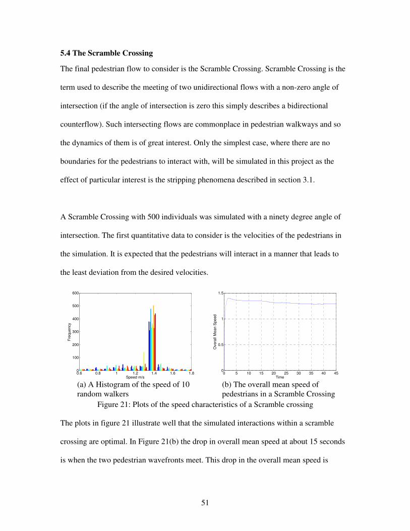
51
5.4 The Scramble Crossing
The final pedestrian flow to consider is the Scramble Crossing. Scramble Crossing is the
term used to describe the meeting of two unidirectional flows with a non-zero angle of
intersection (if the angle of intersection is zero this simply describes a bidirectional
counterflow). Such intersecting flows are commonplace in pedestrian walkways and so
the dynamics of them is of great interest. Only the simplest case, where there are no
boundaries for the pedestrians to interact with, will be simulated in this project as the
effect of particular interest is the stripping phenomena described in section 3.1.
A Scramble Crossing with 500 individuals was simulated with a ninety degree angle of
intersection. The first quantitative data to consider is the velocities of the pedestrians in
the simulation. It is expected that the pedestrians will interact in a manner that leads to
the least deviation from the desired velocities.
0.6 0.8 1 1.2 1.4 1.6 1.80
100
200
300
400
500
600
Speed m/s
Fre
que
ncy
0 5 10 15 20 25 30 35 40 450
0.5
1
1.5
Time
Overa
ll M
ean S
pe
ed
Figure 21: Plots of the speed characteristics of a Scramble crossing
The plots in figure 21 illustrate well that the simulated interactions within a scramble
crossing are optimal. In Figure 21(b) the drop in overall mean speed at about 15 seconds
is when the two pedestrian wavefronts meet. This drop in the overall mean speed is
(a) A Histogram of the speed of 10
random walkers
(b) The overall mean speed of
pedestrians in a Scramble Crossing

52
approximately 0.1 ms-1
which would is clearly not particularly significant. Obviously the
overall mean speed may hide the fact that movement in the area where the 2 flows meet is
very slow. Clearly only a small proportion of the total number of pedestrians will be in
the intersection at any one time and so the speed of the pedestrians outside of the point of
intersection could mask the fact that movement where the flows meet is slow. Figure
21(a) however dispels this; it is a histogram of the speeds at each timestep of a random
sample of 10 pedestrians where each pedestrian is represented by a different colour bar. It
clearly shows that the pedestrian speeds are tightly distributed around the initial desired
speed of 1.34 ms-1
indicating that even when a pedestrian is moving through the area of
intersection their actual speed does not deviate too far from their desired speed.
0 5 10 15 20 25 30 35 40 450
0.05
0.1
0.15
0.2
0.25
0.3
0.35
0.4
0.45
m/s
Time
Variance
Standard Deviation
Figure 22: Variance and Standard Deviation of Pedestrian in a Scramble Crossing
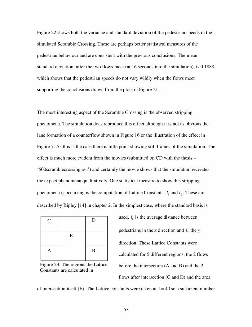
53
C
B A
E
D
Figure 23: The regions the Lattice
Constants are calculated in
Figure 22 shows both the variance and standard deviation of the pedestrian speeds in the
simulated Scramble Crossing. These are perhaps better statistical measures of the
pedestrian behaviour and are consistent with the previous conclusions. The mean
standard deviation, after the two flows meet (at 16 seconds into the simulation), is 0.1888
which shows that the pedestrian speeds do not vary wildly when the flows meet
supporting the conclusions drawn from the plots in Figure 21.
The most interesting aspect of the Scramble Crossing is the observed stripping
phenomena. The simulation does reproduce this effect although it is not as obvious the
lane formation of a counterflow shown in Figure 16 or the illustration of the effect in
Figure 7. As this is the case there is little point showing still frames of the simulation. The
effect is much more evident from the movies (submitted on CD with the thesis –
‘500scramblecrossing.avi’) and certainly the movie shows that the simulation recreates
the expect phenomena qualitatively. One statistical measure to show this stripping
phenomena is occurring is the computation of Lattice Constants, 1 2 and l l . These are
described by Ripley [14] in chapter 2. In the simplest case, where the standard basis is
used, 1l is the average distance between
pedestrians in the x direction and 2l the y
direction. These Lattice Constants were
calculated for 5 different regions, the 2 flows
before the intersection (A and B) and the 2
flows after intersection (C and D) and the area
of intersection itself (E). The Lattice constants were taken at 40t = so a sufficient number
54
of pedestrian had managed to pass the intersection of the flows. The Lattice constants are
summarised in Table 2:
Region 1l 2l
A 0.5486 0.5491
B 0.5516 0.5521
C 0.6132 1.0236
D 0.5962 0.9742
E 0.3212 0.3195
Table 2: Lattice Constants
Initially the pedestrians were uniformly distributed and given the homogeneity of the
walkers in this simulation it is to be expected that the lattice constants in regions A and B
are very close to each other. In region E both the Lattice Constants are close to 0.3 which
is the pedestrian radius defined for this simulation (See Table 1) describing the high
density in the area of intersection. The interesting values are produced in regions C and
D. In these area, 1l , the average separation in the x direction, is close to the initial values
but 2l , the average separation in the y direction has doubled. This change, whilst visually
obvious, provides a quantitative value highlighting the stripping effect.
5.5 Model Shortcomings
Having simulated a variety of pedestrian flows, the results obtained have highlighted a
number of areas in which the model could be improved. The most obvious of these,
which has already being touched upon, is the homogeneity of the system. Currently the
pedestrians are modelled as uniform, which may not be a reasonable assumption and may
lead to important effects not being simulated. The solution would be to obtain further
information on the makeup of pedestrian crowds from experimental data. In the case of
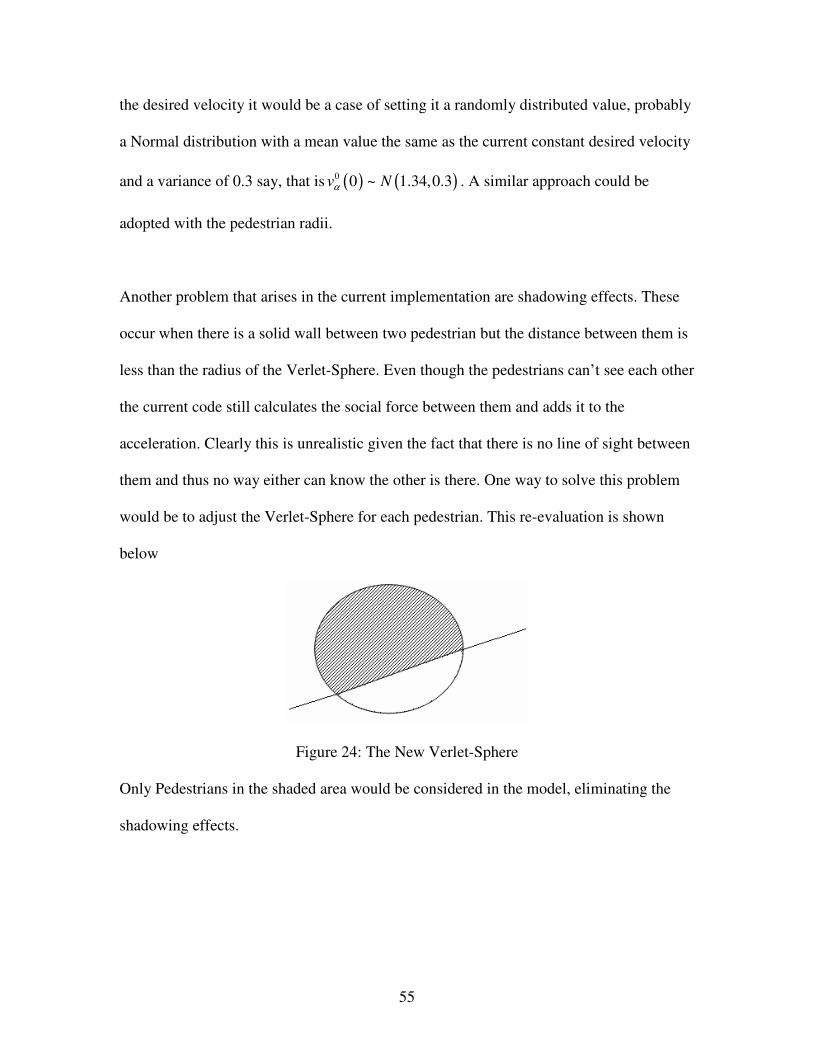
55
the desired velocity it would be a case of setting it a randomly distributed value, probably
a Normal distribution with a mean value the same as the current constant desired velocity
and a variance of 0.3 say, that is ( ) ( )0 0 ~ 1.34,0.3v Nα . A similar approach could be
adopted with the pedestrian radii.
Another problem that arises in the current implementation are shadowing effects. These
occur when there is a solid wall between two pedestrian but the distance between them is
less than the radius of the Verlet-Sphere. Even though the pedestrians can’t see each other
the current code still calculates the social force between them and adds it to the
acceleration. Clearly this is unrealistic given the fact that there is no line of sight between
them and thus no way either can know the other is there. One way to solve this problem
would be to adjust the Verlet-Sphere for each pedestrian. This re-evaluation is shown
below
Figure 24: The New Verlet-Sphere
Only Pedestrians in the shaded area would be considered in the model, eliminating the
shadowing effects.
56
Chapter 6
Summary and Future Directions
The aim of this project was to implement a version of the Social Force Model and use it
to simulate various pedestrian flows. The results produced by the simulation with this
implementation provided some excellent qualitative results, reproducing the expected
self-organisation phenomena very well. These included oscillating flows at bottle necks,
lane formation in a counter flow and stripping in a Scramble Crossing. However in the
final chapter several flaws in the current implementation were identified though solution
to each of them was suggested.
If this project were to be continued in future there are several areas that should be looked
at. The first of these would be to include the additional pedestrian behaviours set out in
section 2.6 such as the random fluctuations described by (2.6.13) and the joining
behaviour discussed in section 2.6.4.
Currently the simulation requires order n2 calculations at each iteration of the ODE
solver. There are techniques to reduce this to an order n algorithm which would allow the
simulation to be run for much larger systems on a single processor. Even if an order n
algorithm is achieved it would be useful to parallelise the implementation so that the
simulation could be extended to huge scale problems such as airport terminals or world
sporting events, where there may be as many as 150,000 pedestrians present.
57
With the order n algorithm in place it would then be possible to explore the effect of
vastly increased density upon the systems already investigated. Certainly in the case of
the ninety degree corner it would be valuable to find a quantitative value for the critical
density of the geometry. The effect of the flow reaching its critical density is of
paramount importance in emergency situations as this is when such a density may be
reached.
Further investigation should focus primarily on the effect of boundaries on pedestrian
flows and try to develop solutions to flaws in current building design. This is simply
because the most interesting pedestrian flows occur when boundaries are present and that
in emergency situations it is the boundaries that become the biggest hazards when they
restrict pedestrian flow.
58
Bibliography
[1] D. Helbing et al. Self-Organized Pedestrian Crowd Dynamics: Experiments,
Simulations, and Design Solutions. Transportation Science, 39(1):1-24, February 2005
[2] D. Helbing and P. Molnár. Social force Model for Pedestrian Dynamics. Physical
Review E, 51(5):4282-4286, May 1995
[3] V. J. Blue and J. L. Adler. Bi-directional Emergent Fundamental Pedestrian Flows
from Cellular Automata Microsimulation. Proceedings of the 14th
International
Symposium of Transportation and Traffic Theory, 1999
[4] L. F. Henderson. The Statistics of Crowd Fluids, Nature, 229:381-383, February 1971
[5] S. Hoogendoorn and P. H. L. Bovy. Gas-Kinetic Modeling and Simulation of
Pedestrian Flows. Transportation Research Record, 1710:28-36, 2000.
[6] S. Okazaki and S. Matsushita. A Study of Simulation Model for Pedestrian Movement
with Evacuation and Queuing. Proceedings of the International Conference on
Engineering for Crowd Safety, pages 271-280, 1993
[7] S. J. Yuhaski, Jr and J. Macgregor Smith. Modeling Circulation Systems in Buildings
Using State Dependent Queuing Models. Queueing Systems, pages 319-338,1989
[8] G. G. Løvas. Modeling and Simulation of Pedestrian Traffic flow. Transportation
Research B, 28(6):429-443, 1994
[9] V. J. Blue and J. L. Adler. Cellular Automata Microsimulation of Bi-Directional
Pedestrian Flows, Transportation Research Record, 1678:135-141, 2000
[10] J. Dijkstra, J. Jessurun and H. Timmermans. A Multi-Agent Cellular Automata
Model of Pedestrian Movement. Pedestrian and Evacuation Dynamics, pages 173-181,
2001
[11] D. Helbing and P. Molnár. Self-Organization Phenomena In Pedestrian Crowds.
Self-Organization of Complex Structures: From Individual to Collective Dynamics, pages
569-577, 1997
[12] J. Dzubiella and H. Löwen. Pattern Formation in Driven Colloidal Mixtures: Tilted
Driving Forces and Re-Entrant Crystal Freezing. J. Physics: Condensed Matter 14:9383-
9395, 2002
[13] L. Verlet. Computer “Experiments” on Classical Fluids. I. Thermodynamical
Properties of Lennard-Jones Molecules. Physical Review, 159(1):98-103
[14] B. D. Ripley. Stochastic Simulation John Wiley & Sons, Inc, 1987
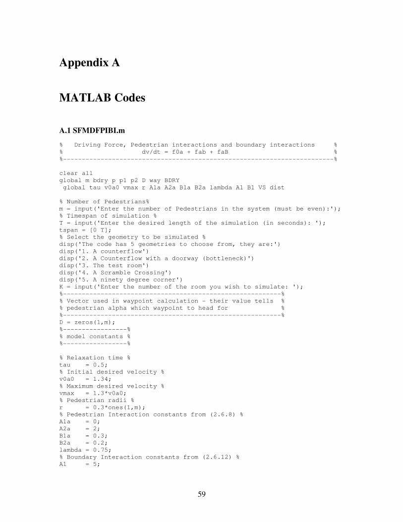
59
Appendix A
MATLAB Codes
A.1 SFMDFPIBI.m
% Driving Force, Pedestrian interactions and boundary interactions %
% dv/dt = f0a + fab + faB %
%------------------------------------------------------------------------%
clear all
global m bdry p p1 p2 D way BDRY
global tau v0a0 vmax r A1a A2a B1a B2a lambda A1 B1 VS dist
% Number of Pedestrians%
m = input('Enter the number of Pedestrians in the system (must be even):');
% Timespan of simulation %
T = input('Enter the desired length of the simulation (in seconds): ');
tspan = [0 T];
% Select the geometry to be simulated %
disp('The code has 5 geometries to choose from, they are:')
disp('1. A counterflow')
disp('2. A Counterflow with a doorway (bottleneck)')
disp('3. The test room')
disp('4. A Scramble Crossing')
disp('5. A ninety degree corner')
K = input('Enter the number of the room you wish to simulate: ');
%----------------------------------------------------------%
% Vector used in waypoint calculation - their value tells %
% pedestrian alpha which waypoint to head for %
%----------------------------------------------------------%
D = zeros(1,m);
%-----------------%
% model constants %
%-----------------%
% Relaxation time %
tau = 0.5;
% Initial desired velocity %
v0a0 = 1.34;
% Maximum desired velocity %
vmax = 1.3*v0a0;
% Pedestrian radii %
r = 0.3*ones(1,m);
% Pedestrian Interaction constants from (2.6.8) %
A1a = 0;
A2a = 2;
B1a = 0.3;
B2a = 0.2;
lambda = 0.75;
% Boundary Interaction constants from (2.6.12) %
A1 = 5;
60
B1 = 0.1;
% Radius of Verlet Sphere %
VS = 10;
% Distance to waypoint at which it deem to have been reached %
dist = 1.2;
%--------------------------------------%
% Initial position and velocity vector %
%--------------------------------------%
if (K == 1)
way = 1;
Vx = [1.34*rand(1,m/2),-1.34*rand(1,m/2)];
Vy = zeros(1,m);
X = [9*rand(1,m/2),9*rand(1,m/2)+11];
Y = [2*rand(1,m)+3.5];
elseif (K == 2)
way = 0;
Vx = zeros(1,m);
Vy = zeros(1,m);
X = [100*rand(1,m/2)-50,100*rand(1,m/2)+50];
Y = [6*rand(1,m)+7.5];
elseif (K == 3)
way = 1;
Vx = zeros(1,m);
Vy = zeros(1,m);
X = [5*rand(1,m/2),5*rand(1,m/2)+15];
Y = [10*rand(1,m)];
elseif (K == 4)
Vx = zeros(1,m);
Vy = zeros(1,m);
X = [45*rand(1,m/2)-40,45*rand(1,m/2)+35];
for i = 1:m
if (i <= m/2)
Y(i) = X(i) - 10*rand(1,1) + 5;
elseif (i > m/2)
Y(i) = (35 - X(i)) + 10*rand(1,1);
end
end
elseif (K == 5)
way = 1;
Vx = zeros(1,m);
Vy = zeros(1,m);
X = [35*rand(1,m)-30];
Y = [2*rand(1,m)+0.5];
end
% Setting u - the initial position and velocity vector %
for i = 1:m
u((2*i)-1) = Vx(i);
u((2*i)) = Vy(i);
end
for i = 1:m
u((2*m)+(2*i)-1) = X(i);
u((2*m)+(2*i)) = Y(i);
end
start = u;
%----------------------------------------------------------------------%
% Desired destination - p is initially set as a waypoint (if required) %
%----------------------------------------------------------------------%
if (K == 1)
61
p = [[10.5*ones(1,m/2),9.5*ones(1,m/2)]',[4.5*ones(1,m)]'];
p1 = [[50*ones(1,(2/0.1)+1)]',[3.5:0.1:5.5]'];
p2 = [[-30*ones(1,(2/0.1)+1)]',[3.5:0.1:5.5]'];
elseif (K == 2)
p = zeros(m,2);
p1 = [[100*ones(1,(6/0.1)+1)]',[7:0.1:13]'];
p2 = [[zeros(1,(6/0.1)+1)]',[7:0.1:13]'];
elseif (K == 3)
p = [[5*ones(1,m/2),15*ones(1,m/2)]',[5*ones(1,m)]'];
p1 = [[20*ones(1,(4/0.1)+1)]',[3:0.1:7]'];
p2 = [[zeros(1,(4/0.1)+1)]',[3:0.1:7]'];
elseif (K == 4)
p = zeros(m,2);
p1 = [[50:0.1:55]',[55:-0.1:50]'];
p2 = [[-15:0.1:-10]',[50:0.1:55]'];
elseif (K == 5)
p = [[8.5*ones(1,m)]',[2*ones(1,m)]'];
p1 = [[7.5:0.1:9.5]',[40*ones(1,(2/0.1)+1)]'];
p2 = [[7.5:0.1:9.5]',[40*ones(1,(2/0.1)+1)]'];
end
%----------------%
% Boundary Array %
%----------------%
if (K == 1)
bdry = [[0:0.1:20,0:0.1:20,10*ones(1,(1/0.1)+1),10*ones(1,(1/0.1)+1)...
]',[3*ones(1,(20/0.1)+1),6*ones(1,(20/0.1)+1),3:0.1:4,5:0.1:6]',];
BDRY = 1;
elseif (K == 2)
bdry = [[-50:0.1:150,-50:0.1:150]'...
,[6*ones(1,(200/0.1)+1),14*ones(1,(200/0.1)+1)]'];
BDRY = 1;
elseif (K == 3)
bdry = [[5:0.1:15,5:0.1:15,5*ones(1,(3/0.1)+1),5*ones(1,(3/0.1)+1)...
,15*ones(1,(3/0.1)+1),15*ones(1,(3/0.1)+1)]'...
,[3*ones(1,(10/0.1)+1),7*ones(1,(10/0.1)+1),0:0.1:3,7:0.1:10,...
0:0.1:3,7:0.1:10]'];
BDRY = 1;
elseif (K == 4)
BDRY = 0;
elseif (K == 5)
bdry = [[-30:0.1:10,-30:0.1:7,10*ones(1,(40/0.1)+1),...
7*ones(1,(37/0.1)+1)]',[zeros(1,(40/0.1)+1),3*ones(1,(37/0.1)+1)...
,0:0.1:40,3:0.1:40]'];
BDRY = 1;
end
%----------------------------------------%
% The solver for the system - here ode45 %
%----------------------------------------%
options1 = odeset('AbsTol',1d-3,'RelTol',1d-4);
[t1,u1] = ode45(@fun5,tspan,start,options1);
pause
%---------------------------------------%
% Plotting the paths of the pedestrians %
%---------------------------------------%
% Plotting the boundaries %
if (K == 4)
hold on
62
else
plot(bdry(:,1),bdry(:,2),'rx')
if (K == 1)||(K==3)
axis([0,20,0,10]);
elseif (K == 2)
axis([25,75,0,20]);
elseif (K == 5)
axis([0,10,0,10]);
end
hold on
end
% Plotting the pedestrian paths %
for i = (2*m)+1:2:(4*m)
if (i<=3*m)
plot(u1(:,i),u1(:,i+1),'b-')
if (K == 1)||(K == 3)
axis([0,20,0,10]);
elseif (K == 2)
axis([25,75,0,20])
elseif K == 4
axis([0,40,0,40]);
elseif K == 5
axis([0,10,0,10]);
end
hold on
else
plot(u1(:,i),u1(:,i+1),'r-')
if (K == 3)||(K ==1)
axis([0,20,0,10]);
elseif (K == 2)
axis([25,75,0,20])
elseif K == 4
axis([0,40,0,40]);
elseif K == 5
axis([0,10,0,10]);
end
hold on
end
end
pause
%-----------------------------------------------------------%
% Making the Movie - plots the pedestrian positions at each %
% timestep and then uses each plot as a movie frame %
%-----------------------------------------------------------%
for j = 1:length(t1)
% Plotting the boundaries %
if (K == 4)
hold off
else
hold off
plot(bdry(:,1),bdry(:,2),'rx')
if (K == 1)||(K == 3)
axis([0,20,0,10]);
elseif (K == 2)
axis([25,75,0,20]);
elseif (K == 5)
axis([0,10,0,10]);
end
hold on
63
end
% Plotting the pedestrians %
for i = (2*m)+1:2:(4*m)
if (i<=3*m)
plot(u1(j,i),u1(j,i+1),'bo')
if (K == 1)||(K == 3)
axis([0,20,0,10]);
elseif (K == 2)
axis([25,75,0,20])
elseif K == 4
axis([0,40,0,40]);
elseif K == 5
axis([0,10,0,10]);
end
hold on
else
plot(u1(j,i),u1(j,i+1),'ro')
if (K == 3)||(K ==1)
axis([0,20,0,10]);
elseif (K == 2)
axis([25,75,20])
elseif K == 4
axis([0,40,0,40]);
elseif K == 5
axis([0,10,0,10]);
end
hold on
end
end
F(j) = getframe;
end
clf
A.2 fun5.m
% Driving force, pedestrian interaction and boundary interaction function %
%-------------------------------------------------------------------------%
function f0a = fun5(t,u)
global m bdry p p1 p2 D way BDRY x0
global tau v0a0 vmax r A1a A2a B1a B2a lambda A1 B1 VS dist
%---------------------------------------------------%
% Putting pedestrian positions in a separate vector %
%---------------------------------------------------%
for i = 1:m
x(i,1) = u((2*i)-1+(2*m));
x(i,2) = u((2*i)+(2*m));
end
%-------------------------------------------------------%
% Setting inital position for average speed calculation %
%-------------------------------------------------------%
if (t == 0)
x0 = x;
end
64
%-------------------------------%
% Desired Velocity from (2.6.6) %
%-------------------------------%
for i = 1:m
if t == 0
v0a(i) = v0a0;
else
V (i,:) = x(i,:) - x0(i,:);
Vbar = norm(V(i,:)/t);
na = 1 - (Vbar/v0a0);
v0a(i) = (1 - na)*v0a0 + na*vmax;
end
%-----------------------%
% Desired destination p %
%-----------------------%
if (way == 1)
% Pedestrians in area A (L-Hand corner for Scramble Crossing) %
if (i <= m/2)
nrmpx(i) = norm(p(i,:) - x(i,:));
if (nrmpx(i) < dist)
D(i) = 1;
end
if (D(i) == 1)
p(i,:) = p1(1,:);
nrmpx(i) = norm(p(i,:) - x(i,:));
for j = 1:length(p1)
if (norm(p1(j,:) - x(i,:)) < nrmpx(i))
p(i,:) = p1(j,:);
nrmpx(i) = norm(p(i,:) - x(i,:));
end
end
end
% Pedestrians in area B (R-Hand corner for Scramble Crossing) %
elseif (i > m/2)
nrmpx(i) = norm(p(i,:) - x(i,:));
if (nrmpx(i) < dist)
D(i) = 1;
end
if (D(i) == 1)
p(i,:) = p2(1,:);
nrmpx(i) = norm(p(i,:) - x(i,:));
for j = 1:length(p2)
if (norm(p2(j,:) - x(i,:)) < nrmpx(i))
p(i,:) = p2(j,:);
nrmpx(i) = norm(p(i,:) - x(i,:));
end
end
end
end
elseif (way == 0)
% Pedestrians in area A (L-Hand corner for Scramble Crossing) %
if (i <= m/2)
p(i,:) = p1(1,:);
nrmpx(i) = norm(p(i,:) - x(i,:));
for j = 1:length(p1)
if (norm(p1(j,:) - x(i,:)) < nrmpx(i))
p(i,:) = p1(j,:);
nrmpx(i) = norm(p(i,:) - x(i,:));
end
65
end
% Pedestrians in area B (R-Hand corner for Scramble Crossing) %
elseif (i > m/2)
p(i,:) = p2(1,:);
nrmpx(i) = norm(p(i,:) - x(i,:));
for j = 1:length(p2)
if (norm(p2(j,:) - x(i,:)) < nrmpx(i))
p(i,:) = p2(j,:);
nrmpx(i) = norm(p(i,:) - x(i,:));
end
end
end
end
%---------------------------------------%
% Desired Direction vector from (2.6.5) %
%---------------------------------------%
if (nrmpx(i) == 0)
e(i,:) = [0,0];
else
e(i,:) = (p(i,:) - x(i,:))/(nrmpx(i));
end
%--------------------------------------%
% Driving Force component from (2.6.4) %
%--------------------------------------%
f((2*i)-1) = ((v0a(i)/tau) * e(i,1)) - (u((2*i)-1)/tau);
f((2*i)) = ((v0a(i)/tau) * e(i,2)) - (u((2*i))/tau);
%---------------------------------------------------------------------%
% Pedestrian Interactions from (2.6.8) - Summing all the interactions %
%---------------------------------------------------------------------%
fab = [0,0];
for j = 1:m
if (i ~= j)
dab = norm(x(i,:) - x(j,:));
if (dab < VS)
rab = r(i) + r(j);
nab = ((x(i,:) - x(j,:))/dab);
fab = fab + ((A1a*exp((rab - dab)/B1a))*nab)...
*(lambda + (1 - lambda)*((1+(-nab*e(i,:)'))/2))...
+ ((A2a*exp((rab - dab)/B2a))*nab);
end
end
end
f((2*i)-1) = f((2*i)-1) + fab(1,1);
f((2*i)) = f((2*i)) + fab(1,2);
%---------------------------------------------------------------------%
% Boundary Interaction component, this is analogous to the pedestrian %
% interactions - infact the formula only needs different constants %
%---------------------------------------------------------------------%
%-----------------------------------------------------%
% Summing all the boundary interactions from (2.6.12) %
%-----------------------------------------------------%
if BDRY == 1
for j = 1:length(bdry)
if (j == 1)
daB = norm(x(i,:) - bdry(j,:));
BDY = bdry(j,:);
rd = r(i) - daB;
elseif ((norm(x(i,:) - bdry(j,:))) < daB)
daB = norm(x(i,:) - bdry(j,:));
66
BDY = bdry(j,:);
rd = r(i) - daB;
end
end
naB = (x(i,:) - BDY)/daB;
faB = ((A1*exp(rd/B1))*naB);
f((2*i)-1) = f((2*i)-1) + faB(1,1);
f((2*i)) = f((2*i)) + faB(1,2);
end
%----------------------------------%
% Displacement update from (2.6.1) %
%----------------------------------%
X((2*i)-1)= u((2*i)-1);
X(2*i) = u(2*i);
end
f0a = [f,X]';


