HIGH CONTRAST TANDEM FABRY-PÉROT INTERFEROMETER

TFP-2 HC

Operator Manual

Im Grindel 6 8932 Mettmenstetten-Switzerland Phone: +41 (0) 44 776 33 66 Fax: +41 (0) 44 776 33 65 E-Mail: info@tablestable.com Internet: www.tablestable.com

2

Table of contents Safety instructions ................................................................................................................... 4 1 INTRODUCTION TO FABRY-PÉROT INTERFEROMETRY ............................................... 5

1.1 Properties of Fabry-Pérot Interferometer ...................................................................... 5 1.2 Traditional Design of FP and Related Problems ........................................................... 6

1.2.1 Non-linear scan ......................................................................................................... 7 1.2.2 Mirror tilt .................................................................................................................... 7 1.2.3 Tedious to change mirror spacing ............................................................................. 7 1.2.4 Stability ..................................................................................................................... 7 1.2.5 The device is not suited for tandem operation ........................................................... 7

1.3 Novel Parallelogram Construction ................................................................................ 8 1.3.1 The compound translation stage ............................................................................... 9 1.3.2 Measurement transducer for mirror spacing .............................................................. 9

1.4 Tandem Interferometry ............................................................................................... 10 1.5 A practical Design of Scanning Tandem FP................................................................ 11 1.6 Vibration Isolation ....................................................................................................... 13 1.7 Prealignment of the Interferometer ............................................................................. 14 1.8 Stabilizing the Fabry-Pérot ......................................................................................... 15 1.9 Improved Optical Path for High Contrast Operation in the TFP-2 HC ......................... 15

2 OPTICAL SYSTEM FOR TANDEM TRIPLE-PASS OPERATION .................................... 16 2.1 Description of the New High Contrast Optics for the TFP-2 HC .................................. 16 2.2 Quarter Wave Optics .................................................................................................. 16 2.3 Description of the Optical System ............................................................................... 18

2.3.1 Tandem mode optics description............................................................................. 18 2.3.2 Alignment mode optics description .......................................................................... 18

2.4 Rotating Notch Filter Usage (for use with the CM-1 Microscope Appendix) ................ 20 3 ASSEMBLY AND OPERATION OF INTERFEROMETER ................................................ 21

3.1 Instrument Unpacking and Checking .......................................................................... 21 3.1.1 Adjustment or reset of transducer ........................................................................... 22 3.1.2 Further check of control unit .................................................................................... 23

3.2 Operation of Isolation System ..................................................................................... 24 3.3 Mounting the Mirrors in the Interferometer .................................................................. 25 3.4 Instrument Block Diagram and Connections ............................................................... 27

3.4.1 Interferometer control unit ....................................................................................... 28 3.4.2 Interferometer control unit rear panel connectors .................................................... 30 3.4.3 Controls available on the interferometer enclosure ................................................. 31 3.4.4 Familiarizing yourself with the tandem interferometer .............................................. 32 3.4.5 Use of the detector and of the MCA GHOST data gathering system ....................... 33 3.4.6 Changing the mirror spacing ................................................................................... 33 3.4.7 Motor compensation of PZT drift ............................................................................. 34 3.4.8 Learning to use the scan control ............................................................................. 34 3.4.9 Window operation ................................................................................................... 37 3.4.10 Scanning the Tandem Interferometer ...................................................................... 38

3.5 A Test to Check the Correct Operation of the System ................................................ 40 3.6 Some Notes for Starting a New Measurement ............................................................ 40 3.7 Photon Counting Limit, Detector Linearity and Saturation ........................................... 41 3.8 Polarisation Selectivity in the TFP-2 HC ..................................................................... 42 3.9 Alignment of Optical System and Occasional Checks ................................................. 42 3.10 Choice of Pinhole Size ............................................................................................... 43 3.11 Optics for Backscattering ............................................................................................ 44 3.12 Calibration of Mirror Spacings .................................................................................... 45

4 USER ADJUSTMENTS OF ELECTRONICS ..................................................................... 46

3

4.1 Adjustment of Scan Board .......................................................................................... 46 4.2 Further Adjustments ................................................................................................... 48

4.2.1 Adjustment of LCD display of scan amplitude ......................................................... 48 4.2.2 Adjusting the Z scan movement ............................................................................ 48

4.3 Adjustment of Capacitance Range and Centring of Scan Amplitude Indicator ............ 49 4.4 Control Unit - External Connectors ............................................................................. 51 4.5 Interferometer Control Unit Remote Control Inputs ..................................................... 53

5 CIRCUIT DIAGRAMS ........................................................................................................ 54 5.1 Scan Board................................................................................................................. 54 5.2 Stabiliser Memory ....................................................................................................... 55 5.3 PZT Driver Circuitry .................................................................................................... 56 5.4 HV Amplifier ............................................................................................................... 57

6 TROUBLESHOOTING ...................................................................................................... 58 7 APPENDIX ........................................................................................................................ 61

7.1 Specifications of Tandem Fabry-Pérot Interferometer ................................................. 61 7.2 Preparing the TFP-2 HC Interferometer for Shipping .................................................. 62 7.3 A Light Source for Alignment and Calibration ............................................................. 66 7.4 Alignment of Reference Beam .................................................................................... 68

7.4.1 Alternative alignment procedure .............................................................................. 69 7.5 Alignment of Optics .................................................................................................... 70 7.6 Fine Check of Incidence Angles Using Interference Fringes ....................................... 78 7.7 Calibration of Mirror Spacings .................................................................................... 79

7.7.1 First calibration of mirrors spacings using interference rings ................................... 79 7.7.2 Precise calibration of mirror spacings using conical lens, gauge adjustment ........... 82

7.8 Cleaning the Mirrors ................................................................................................... 85

V-1703/1.5

4

SAFETY INSTRUCTIONS The system may only be plugged into a socket with separate ground. Do not disconnect this ground, either at the socket, or by using an ungrounded extension cable. If you suspect the system to be in any way unsafe, unplug and prevent any possible accidental usage. Contact your nearest service centre. Before switching on this apparatus make sure that it is connected to the correct mains voltage. Do not remove any cover or allow any metal objects to enter the ventilation slits. Disconnect from mains before removing any covers. Refer servicing to qualified personnel. Do not use in potentially explosive surroundings. The fuses are located in the power socket on the rear side of the control unit. Do not attempt to change a fuse without first unplugging from the mains. Only replace a fuse with the correct type. Never try to bypass a fuse. Make sure the ventilation slits in the control unit are not covered and that air can freely circulate. Blocking the slits can lead to overheating which could cause a fire.

5

1 INTRODUCTION TO FABRY-PÉROT INTERFEROMETRY

1.1 Properties of Fabry-Pérot Interferometer

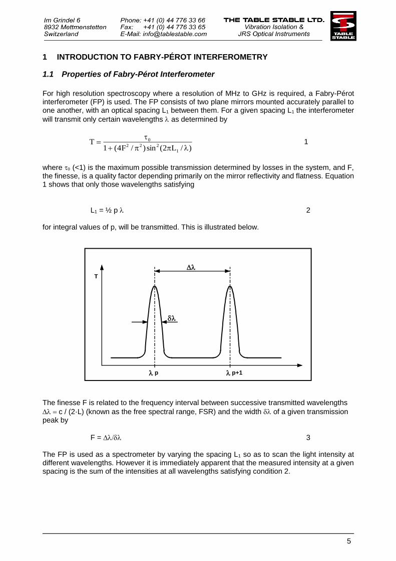
For high resolution spectroscopy where a resolution of MHz to GHz is required, a Fabry-Pérot interferometer (FP) is used. The FP consists of two plane mirrors mounted accurately parallel to one another, with an optical spacing L1 between them. For a given spacing L1 the interferometer

will transmit only certain wavelengths as determined by

)/L2(sin)/F4(1T

1

222

0

1

where (<1) is the maximum possible transmission determined by losses in the system, and F, the finesse, is a quality factor depending primarily on the mirror reflectivity and flatness. Equation 1 shows that only those wavelengths satisfying

L1 = ½ p 2 for integral values of p, will be transmitted. This is illustrated below.

T

p+1

p

The finesse F is related to the frequency interval between successive transmitted wavelengths

c / (2·L) (known as the free spectral range, FSR) and the width of a given transmission peak by

F = 3 The FP is used as a spectrometer by varying the spacing L1 so as to scan the light intensity at different wavelengths. However it is immediately apparent that the measured intensity at a given spacing is the sum of the intensities at all wavelengths satisfying condition 2.

6

An unambiguous interpretation of the spectrum is thus impossible unless it is known a priori that

the spectrum of the light lies entirely within a wavelength spread < It is true that since

/2L1 4

one may make arbitrarily large by decreasing L1. However increases proportional to and

so the resolution decreases. In fact equation 3 shows that the ratio between FSR, and the

resolution is just the finesse F. In practice F cannot be made much greater than about 100 due to limitations on the quality of mirror substrates and coatings. The relationship between FSR and resolution is thus fixed within limits determined by the achievable values of F.

1.2 Traditional Design of FP and Related Problems

A design of scanning Fabry-Pérot commonly used in the past is illustrated in Figure 1-1. The structure is based upon 3 low expansion rods which support the 3 piezoelectric scanning stacks. One mirror is attached in some suitable strain-free manner to the ends of the 3 scanning stacks. The second mirror is attached to the end plate of the structure in such a way that approximate alignment parallel to the first mirror may be achieved by means of differential micrometer screws. Exact alignment of the mirrors is achieved by applying suitable bias voltages to the three scanning stacks. The instrument is then scanned by applying a scanning voltage simultaneously to all 3 scanning stacks.

Figure 1-1

ALIGNEMENT

SCREWS

FIXED MIRRORS

SCANNING MIRROR

SCANNING STACK

(1 OF 3)

While such a device can operate quite successfully under some conditions there are several aspects where considerable improvement is to be desired. These are discussed below.

7

1.2.1 Non-linear scan

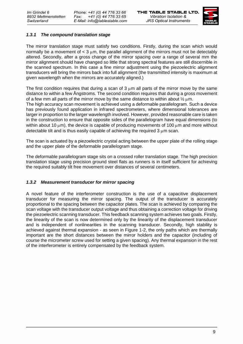
Since piezoelectric transducers are somewhat non-linear, the scan produced is not linearly proportional to the scan voltage.

1.2.2 Mirror tilt

Piezoelectric transducers are not entirely homogeneous and so the three scanning stacks do not have identical characteristics. As a result the three stacks do not produce identical displacements and so the mirror tilts during the scan. This loss of parallel mirror alignment is serious for multipass operation of the interferometer.

1.2.3 Tedious to change mirror spacing

The mirror spacing determines the resolution of the interferometer. When the mirror spacing must be changed the scanning mirror assembly must be slid as a whole along the three rods. As a result mirror alignment is lost and the handling produces local temperature changes. The mirrors must be realigned with the micrometer screws and finally with the bias voltages on the scanning stacks. Time must be allowed for the instrument to thermalise again. The coarse mirror alignment is particularly time consuming and the whole process very inconvenient.

1.2.4 Stability

The mean mirror spacing and the parallel alignment should not vary with time. This requires dimensional stabilities of the order of 20 Å. To meet this requirement it is necessary to build the instrument out of low expansion materials which are expensive both to buy and to machine.

1.2.5 The device is not suited for tandem operation

The combination of non-linearity in the scan and rather poor stability makes the synchronous operation of two interferometers in tandem virtually impossible. In the following a method of constructing an interferometer is described using techniques which are known in other fields but which have not previously been applied to this problem. The resulting instrument gives a very satisfactory solution to all of the above problems.

8

1.3 Novel Parallelogram Construction

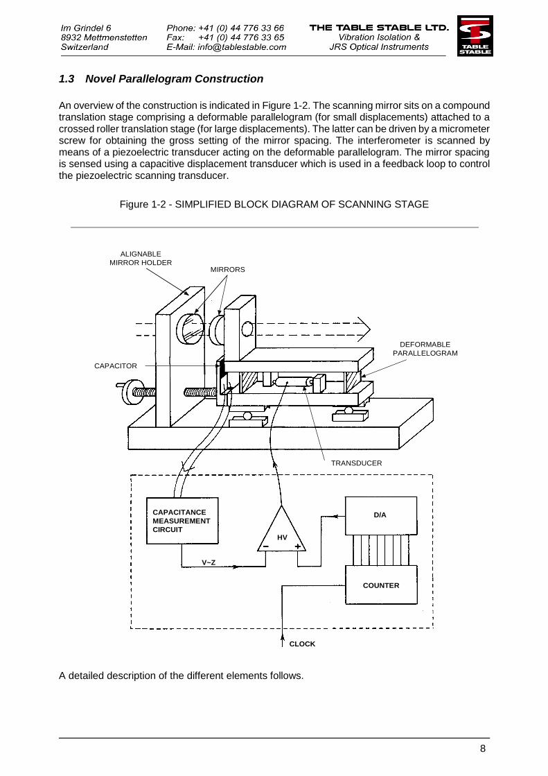
An overview of the construction is indicated in Figure 1-2. The scanning mirror sits on a compound translation stage comprising a deformable parallelogram (for small displacements) attached to a crossed roller translation stage (for large displacements). The latter can be driven by a micrometer screw for obtaining the gross setting of the mirror spacing. The interferometer is scanned by means of a piezoelectric transducer acting on the deformable parallelogram. The mirror spacing is sensed using a capacitive displacement transducer which is used in a feedback loop to control the piezoelectric scanning transducer.

Figure 1-2 - SIMPLIFIED BLOCK DIAGRAM OF SCANNING STAGE

MIRRORS

ALIGNABLE

MIRROR HOLDER

DEFORMABLE

PARALLELOGRAM

TRANSDUCER

CAPACITOR

CAPACITANCE

MEASUREMENT

CIRCUIT

D/A

COUNTER

CLOCK

V~Z

HV

A detailed description of the different elements follows.

9

1.3.1 The compound translation stage

The mirror translation stage must satisfy two conditions. Firstly, during the scan which would

normally be a movement of < 3 m, the parallel alignment of the mirrors must not be detectably altered. Secondly, after a gross change of the mirror spacing over a range of several mm the mirror alignment should have changed so little that strong spectral features are still discernible in the scanned spectrum. In this case a fine mirror adjustment using the piezoelectric alignment transducers will bring the mirrors back into full alignment (the transmitted intensity is maximum at given wavelength when the mirrors are accurately aligned.)

The first condition requires that during a scan of 3 m all parts of the mirror move by the same distance to within a few Ångstroms. The second condition requires that during a gross movement

of a few mm all parts of the mirror move by the same distance to within about ½ m. The high accuracy scan movement is achieved using a deformable parallelogram. Such a device has previously found application in infrared spectrometers, where dimensional tolerances are larger in proportion to the larger wavelength involved. However, provided reasonable care is taken in the construction to ensure that opposite sides of the parallelogram have equal dimensions (to

within about 10 m), the device is capable of producing movements of 100m and more without

detectable tilt and is thus easily capable of achieving the required 3 m scan. The scan is actuated by a piezoelectric crystal acting between the upper plate of the rolling stage and the upper plate of the deformable parallelogram stage. The deformable parallelogram stage sits on a crossed roller translation stage. The high precision translation stage using precision ground steel flats as runners is in itself sufficient for achieving the required suitably tilt free movement over distances of several centimeters.

1.3.2 Measurement transducer for mirror spacing

A novel feature of the interferometer construction is the use of a capacitive displacement transducer for measuring the mirror spacing. The output of the transducer is accurately proportional to the spacing between the capacitor plates. The scan is achieved by comparing the scan voltage with the transducer output voltage and thus obtaining a correction voltage for driving the piezoelectric scanning transducer. This feedback scanning system achieves two goals. Firstly, the linearity of the scan is now determined only by the linearity of the displacement transducer and is independent of nonlinearities in the scanning transducer. Secondly, high stability is achieved against thermal expansion - as seen in Figure 1-2, the only paths which are thermally important are the short distances between the mirror holders and the capacitor (including of course the micrometer screw used for setting a given spacing). Any thermal expansion in the rest of the interferometer is entirely compensated by the feedback system.

10

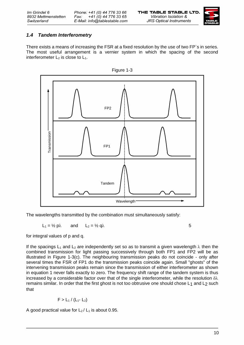
1.4 Tandem Interferometry

There exists a means of increasing the FSR at a fixed resolution by the use of two FP`s in series. The most useful arrangement is a vernier system in which the spacing of the second interferometer L2 is close to L1.

Figure 1-3

FP2

FP1

Tandem

Tra

nsm

issio

n

Wavelength

The wavelengths transmitted by the combination must simultaneously satisfy:

L1 = ½ p and L2 = ½ q 5 for integral values of p and q.

If the spacings L1 and L2 are independently set so as to transmit a given wavelength then the combined transmission for light passing successively through both FP1 and FP2 will be as illustrated in Figure 1-3(c). The neighbouring transmission peaks do not coincide - only after several times the FSR of FP1 do the transmission peaks coincide again. Small "ghosts" of the intervening transmission peaks remain since the transmission of either interferometer as shown in equation 1 never falls exactly to zero. The frequency shift range of the tandem system is thus

increased by a considerable factor over that of the single interferometer, while the resolution remains similar. In order that the first ghost is not too obtrusive one should chose L1 and L2 such

that F > L1 / (L1- L2) A good practical value for L2 / L1 is about 0.95.

11

To use the tandem interferometer system as a spectrometer, it is necessary to scan the two interferometers synchronously, by simultaneously changing the spacings L1 and L2. It is clear from

equations 2 and 5 that to scan a given wavelength increment, the changes L1 and L2 must satisfy

L1 / L2 = L1 / L2 6

The magnitudes of L1 and L2 are typically 1 to a few m. The only previously known method of satisfying 6 was by use of pressure scanning. Remembering that L is the optical spacing of the mirrors (i.e. the spacing t multiplied by the refractive index n of the gas between the mirrors) one may change L by changing the refractive index of the gas through a pressure change. Since L1 = n·t1 and L2 = n·t2 we see that condition 6 will be satisfied if the refractive index change is the same for both interferometers. The limitation of the method lies in the scanning range which is limited by the achievable refractive index change. Using air, a pressure change of 1 atmosphere will change L by only 3 parts in 104, producing the same relative change in the transmitted wavelengths. Where much larger scans are required, the associated large pressure changes make the system impracticable. Any practical construction of a tandem scanning interferometer, apart from having a large scan range, must satisfy the following criteria: Static synchronization Synchronization requires that the spacings of the two interferometers are never allowed to depart from their correct relative values by as much as 20 Å. Dynamic synchronization

The correct relative spacings must be maintained over a scan of several m.

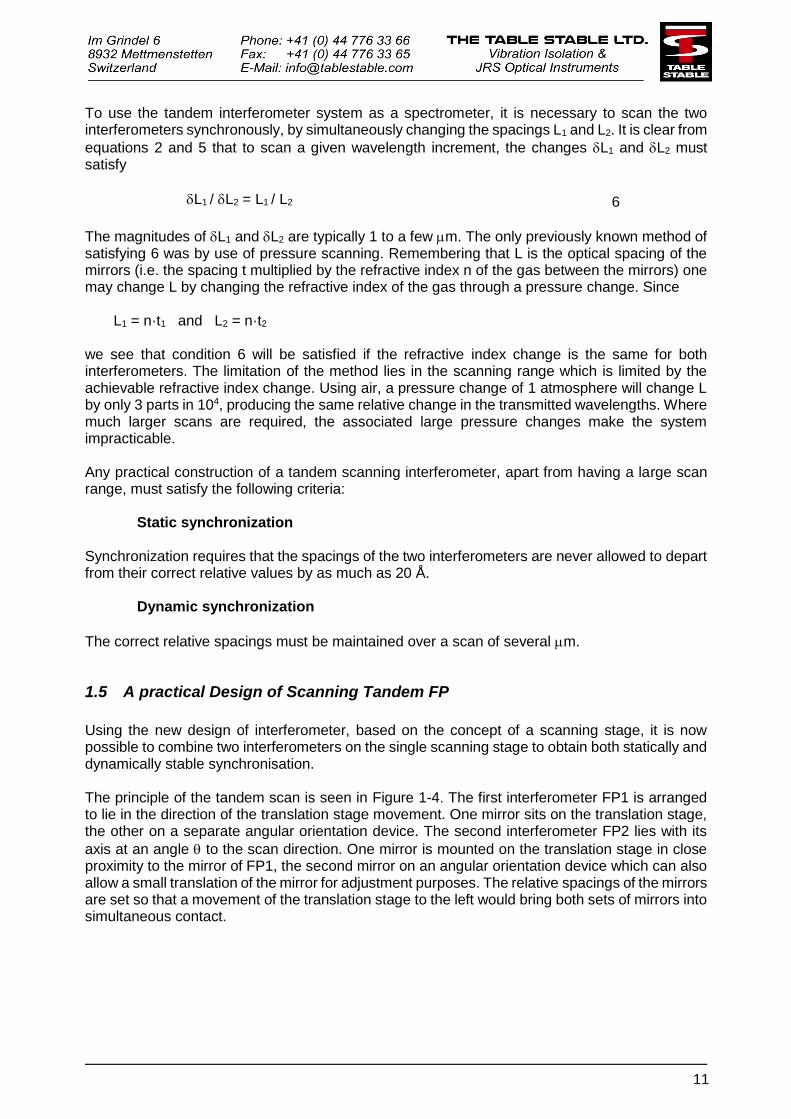
1.5 A practical Design of Scanning Tandem FP

Using the new design of interferometer, based on the concept of a scanning stage, it is now possible to combine two interferometers on the single scanning stage to obtain both statically and dynamically stable synchronisation. The principle of the tandem scan is seen in Figure 1-4. The first interferometer FP1 is arranged to lie in the direction of the translation stage movement. One mirror sits on the translation stage, the other on a separate angular orientation device. The second interferometer FP2 lies with its

axis at an angle to the scan direction. One mirror is mounted on the translation stage in close proximity to the mirror of FP1, the second mirror on an angular orientation device which can also allow a small translation of the mirror for adjustment purposes. The relative spacings of the mirrors are set so that a movement of the translation stage to the left would bring both sets of mirrors into simultaneous contact.

12

A movement of the translation stage to the right sets the spacings to L1 and L1·cos . A scan L1

of the translation stage produces a change of spacing L1 in FP1 and L1·cos in FP2. In other words relation 6 is satisfied and so the two interferometers scan synchronously. An upper limit on the length of the scan is imposed by the shear displacement of the mirrors of FP2 - after a scan

of more than D/sin (mirror diameter D) the mirrors would no longer overlap. A scan of several cm is easily possible for normal mirror diameters (3÷5 cm). Since the scan lengths in practice

rarely exceeds 3 m this large range should rather be understood as the range over which L1 may be adjusted without requiring a lateral repositioning of one of the mirrors of FP2.

Figure 1-4

FP2

FP1

DIRECTION OF

MOVEMENT

L1

L2 = L1cos

TRANSLATION

STAGE

The main features of the system are:

- Complete dynamic synchronization over a large scanning range. - Good static synchronization due to the compact design which enables both interferometers to share the same environment.

13

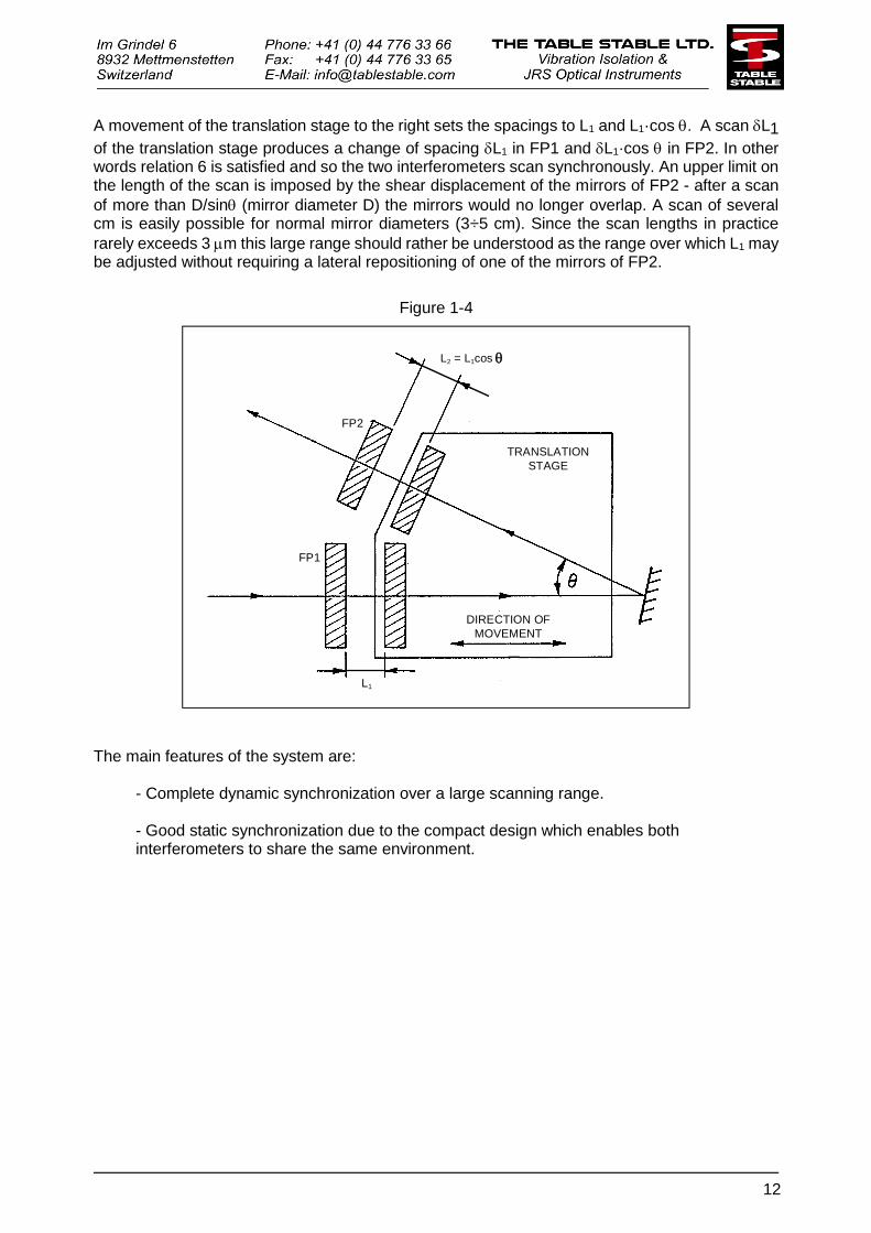
1.6 Vibration Isolation

The interferometer requires a quiet, vibration free environment. In order to scan a Fabry-Pérot through a single transmission peak a change in mirror spacing of about 25 Å is required. It is apparent that any external influence which distorts the mirror spacing by more than a few Å will seriously degrade the spectrum. Building vibrations, which typically have their maximum amplitudes in the range 10-20 Hz, introduce non-resonant distortions of the interferometer which can make the operation of the spectrometer impossible. The traditional solution to vibration problems is to isolate the complete optical system from the building by using very soft passive springs in the form of damped air columns. Such a solution is adequate, but has the disadvantage that any vibration sources placed directly on the optical table will, of course, not be isolated from the interferometer. The better solution is to mount the optical table rigidly on the floor, but to isolate the interferometer from the optical table. Dynamic isolation systems, using feedback control have recently become available and are ideal for this application. They are compact, stiff and with excellent directional and positional stability, unlike the soft passive isolation systems which drift over large displacements at low frequency. Figure 1-5 shows the tandem interferometer mounted on two dynamical isolation mounts. The optical components for multi-passing the interferometer are mounted directly on the optical table, since these components are, in general, not sensitive to building vibrations. Note that an enclosure is required around the interferometer to protect it from sound waves which can excite high-frequency resonances in the system.

Figure 1-5

Interferometer shown supported by active isolation system AVI-35 LPR

FP1

FP2

TRANSLATIONSTAGE

AVI-35 LPR ELEMENTS

14

1.7 Prealignment of the Interferometer

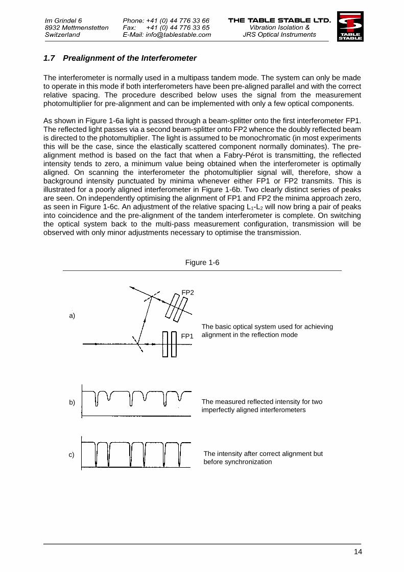
The interferometer is normally used in a multipass tandem mode. The system can only be made to operate in this mode if both interferometers have been pre-aligned parallel and with the correct relative spacing. The procedure described below uses the signal from the measurement photomultiplier for pre-alignment and can be implemented with only a few optical components. As shown in Figure 1-6a light is passed through a beam-splitter onto the first interferometer FP1. The reflected light passes via a second beam-splitter onto FP2 whence the doubly reflected beam is directed to the photomultiplier. The light is assumed to be monochromatic (in most experiments this will be the case, since the elastically scattered component normally dominates). The pre-alignment method is based on the fact that when a Fabry-Pérot is transmitting, the reflected intensity tends to zero, a minimum value being obtained when the interferometer is optimally aligned. On scanning the interferometer the photomultiplier signal will, therefore, show a background intensity punctuated by minima whenever either FP1 or FP2 transmits. This is illustrated for a poorly aligned interferometer in Figure 1-6b. Two clearly distinct series of peaks are seen. On independently optimising the alignment of FP1 and FP2 the minima approach zero, as seen in Figure 1-6c. An adjustment of the relative spacing L1-L2 will now bring a pair of peaks into coincidence and the pre-alignment of the tandem interferometer is complete. On switching the optical system back to the multi-pass measurement configuration, transmission will be observed with only minor adjustments necessary to optimise the transmission.

Figure 1-6

FP2

FP1

The basic optical system used for achieving

alignment in the reflection mode

The measured reflected intensity for two

imperfectly aligned interferometers

The intensity after correct alignment but

before synchronization

a)

b)

c)

15

1.8 Stabilizing the Fabry-Pérot

In order to obtain long time stability of an interferometer it is necessary to apply some form of dynamic control in order to maintain both parallel alignment of the mirrors and correct spacing. The means by which this is achieved for a single interferometer is described at length in J.Phys.E, 9 (1976) p. 566. Four successive scans are required in order to obtain error and correction signals for the two axes X and Y to maintain parallelism in a single interferometer. A tandem interferometer system requires many more scans in order to obtain the appropriate correction signals because now

correct alignment involves adjustments about 5 axes, namely X1, Y1, X2, Y2 and Z, where Z

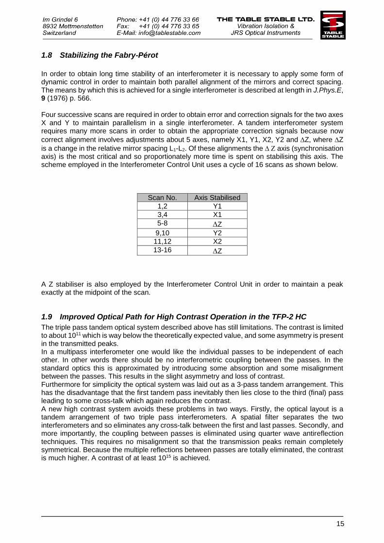
is a change in the relative mirror spacing L1-L2. Of these alignments the axis (synchronisation axis) is the most critical and so proportionately more time is spent on stabilising this axis. The scheme employed in the Interferometer Control Unit uses a cycle of 16 scans as shown below.

Scan No. Axis Stabilised

1,2 Y1

3,4 X1

5-8 Z

9,10 Y2

11,12 X2

13-16 Z

A Z stabiliser is also employed by the Interferometer Control Unit in order to maintain a peak exactly at the midpoint of the scan.

1.9 Improved Optical Path for High Contrast Operation in the TFP-2 HC

The triple pass tandem optical system described above has still limitations. The contrast is limited to about 1011 which is way below the theoretically expected value, and some asymmetry is present in the transmitted peaks. In a multipass interferometer one would like the individual passes to be independent of each other. In other words there should be no interferometric coupling between the passes. In the standard optics this is approximated by introducing some absorption and some misalignment between the passes. This results in the slight asymmetry and loss of contrast. Furthermore for simplicity the optical system was laid out as a 3-pass tandem arrangement. This has the disadvantage that the first tandem pass inevitably then lies close to the third (final) pass leading to some cross-talk which again reduces the contrast. A new high contrast system avoids these problems in two ways. Firstly, the optical layout is a tandem arrangement of two triple pass interferometers. A spatial filter separates the two interferometers and so eliminates any cross-talk between the first and last passes. Secondly, and more importantly, the coupling between passes is eliminated using quarter wave antireflection techniques. This requires no misalignment so that the transmission peaks remain completely symmetrical. Because the multiple reflections between passes are totally eliminated, the contrast is much higher. A contrast of at least 1015 is achieved.

16

2 OPTICAL SYSTEM FOR TANDEM TRIPLE-PASS OPERATION The optical system allows the interferometer to be used in the high contrast tandem triple-pass mode and in an alternative mirror alignment configuration. The system has been designed using a minimum number of components and is shown schematically in Figure 2-3 (tandem configuration) and Figure 2-4 (alignment configuration). Refer to these figures for the meaning of the components abbreviation used in this section of the manual. Some of the components used in the system and here described are protected by the internal dark screens and will not be immediately visible when the instrument lid is open.

2.1 Description of the New High Contrast Optics for the TFP-2 HC

The standard triple pass tandem optical system used in the interferometer TFP-1 has its limitations. The contrast is limited to about 1011 which is way below the theoretically expected value, and some asymmetry is present in the transmitted peaks. In a multipass interferometer one would like the individual passes to be independent of each other. In other words there should be no interferometric coupling between the passes. In the standard optics this is approximated by introducing some absorption and some misalignment between the passes. This results in the slight asymmetry and loss of contrast. Furthermore the standard optical system is laid out as a 3-pass tandem arrangement. The first tandem pass inevitably then lies close to the third pass leading to some cross-talk which again reduces the contrast. The new high contrast optics avoids these problems in two ways. Firstly the optical arrangement is a tandem arrangement of two triple pass interferometers. A spatial filter separates the two interferometers and so eliminates any cross-talk between the first and last passes. Secondly and more importantly, the coupling between passes is eliminated using quarter wave retardation techniques. This requires no misalignment so that the transmission peaks remain completely symmetrical. Because the multiple reflections between passes are totally eliminated, the contrast is much higher. A contrast of at least 1015 is achieved.

2.2 Quarter Wave Optics

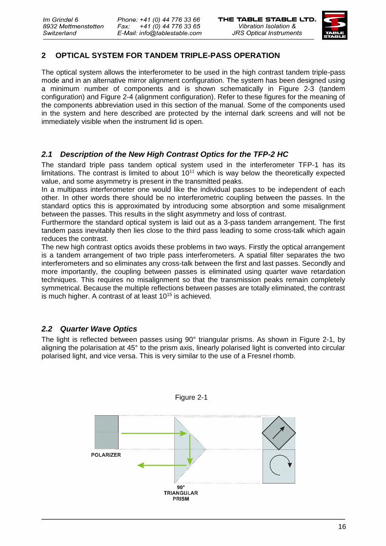
The light is reflected between passes using 90° triangular prisms. As shown in Figure 2-1, by aligning the polarisation at 45° to the prism axis, linearly polarised light is converted into circular polarised light, and vice versa. This is very similar to the use of a Fresnel rhomb.

Figure 2-1

17

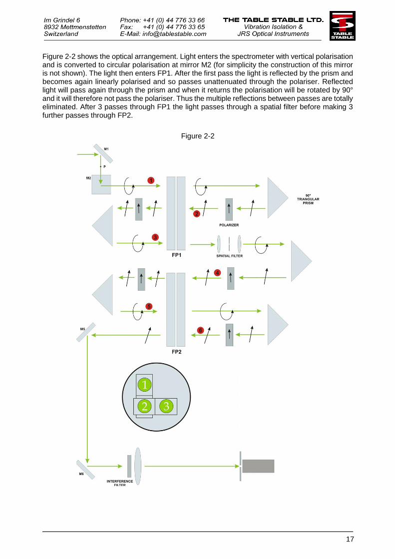
Figure 2-2 shows the optical arrangement. Light enters the spectrometer with vertical polarisation and is converted to circular polarisation at mirror M2 (for simplicity the construction of this mirror is not shown). The light then enters FP1. After the first pass the light is reflected by the prism and becomes again linearly polarised and so passes unattenuated through the polariser. Reflected light will pass again through the prism and when it returns the polarisation will be rotated by 90° and it will therefore not pass the polariser. Thus the multiple reflections between passes are totally eliminated. After 3 passes through FP1 the light passes through a spatial filter before making 3 further passes through FP2.

Figure 2-2

18

2.3 Description of the Optical System

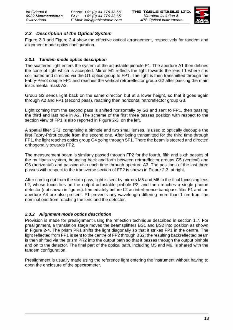
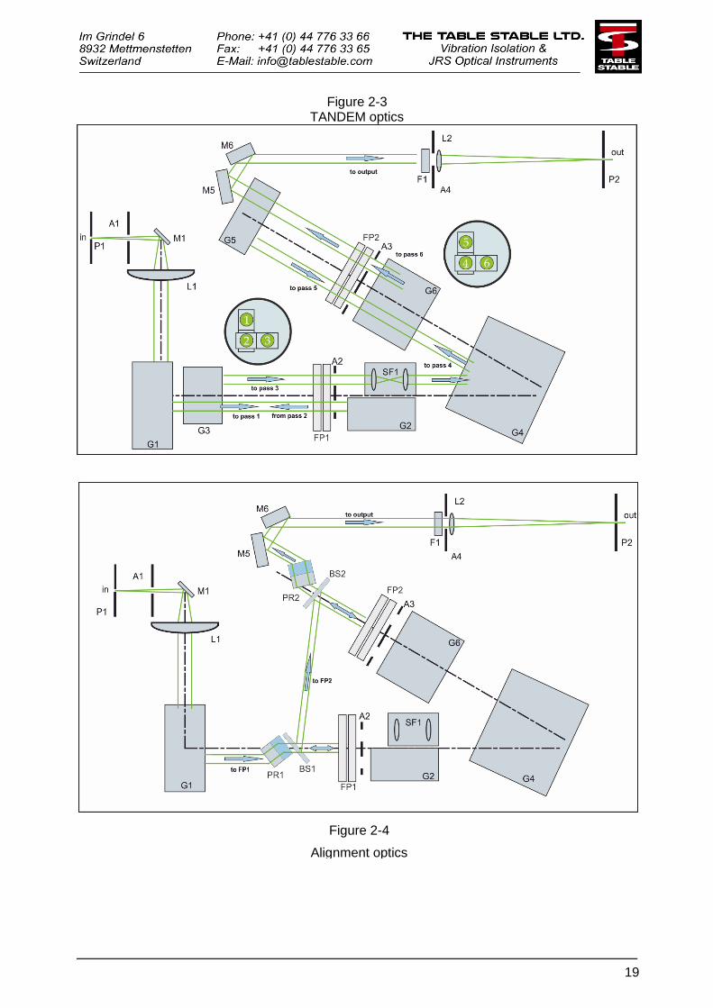
Figure 2-3 and Figure 2-4 show the effective optical arrangement, respectively for tandem and alignment mode optics configuration.

2.3.1 Tandem mode optics description

The scattered light enters the system at the adjustable pinhole P1. The aperture A1 then defines the cone of light which is accepted. Mirror M1 reflects the light towards the lens L1 where it is collimated and directed via the G1 optics group to FP1. The light is then transmitted through the Fabry-Pérot couple FP1 and reaches the vertical retroreflector group G2 after passing the main instrumental mask A2. Group G2 sends light back on the same direction but at a lower height, so that it goes again through A2 and FP1 (second pass), reaching then horizontal retroreflector group G3. Light coming from the second pass is shifted horizontally by G3 and sent to FP1, then passing the third and last hole in A2. The scheme of the first three passes position with respect to the section view of FP1 is also reported in Figure 2-3, on the left. A spatial filter SF1, comprising a pinhole and two small lenses, is used to optically decouple the first Fabry-Pérot couple from the second one. After being transmitted for the third time through FP1, the light reaches optics group G4 going through SF1. There the beam is steered and directed orthogonally towards FP2. The measurement beam is similarly passed through FP2 for the fourth, fifth and sixth passes of the multipass system, bouncing back and forth between retroreflector groups G5 (vertical) and G6 (horizontal) and passing also each time through aperture A3. The positions of the last three passes with respect to the transverse section of FP2 is shown in Figure 2-3, at right. After coming out from the sixth pass, light is sent by mirrors M5 and M6 to the final focussing lens L2, whose focus lies on the output adjustable pinhole P2, and then reaches a single photon detector (not shown in figures). Immediately before L2 an interference bandpass filter F1 and an aperture A4 are also present. F1 prevents any wavelength differing more than 1 nm from the nominal one from reaching the lens and the detector.

2.3.2 Alignment mode optics description

Provision is made for prealignment using the reflection technique described in section 1.7. For prealignment, a translation stage moves the beamsplitters BS1 and BS2 into position as shown in Figure 2-4. The prism PR1 shifts the light diagonally so that it strikes FP1 in the centre. The light reflected from FP1 is sent to the centre of FP2 through BS2; the resulting backreflected beam is then shifted via the prism PR2 into the output path so that it passes through the output pinhole and on to the detector. The final part of the optical path, including M5 and M6, is shared with the tandem configuration. Prealignment is usually made using the reference light entering the instrument without having to open the enclosure of the spectrometer.

19

Figure 2-3 TANDEM optics

Figure 2-4

Alignment optics

20

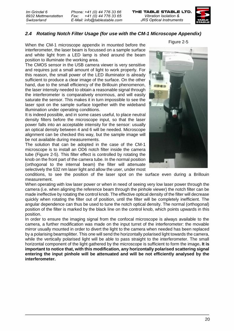
2.4 Rotating Notch Filter Usage (for use with the CM-1 Microscope Appendix)

When the CM-1 microscope appendix in mounted before the interferometer, the laser beam is focussed on a sample surface and white light from a LED lamp is shed around the beam position to illuminate the working area. The CMOS sensor in the USB camera viewer is very sensitive and requires just a small amount of light to work properly. For this reason, the small power of the LED illuminator is already sufficient to produce a clear image of the surface. On the other hand, due to the small efficiency of the Brillouin phenomenon, the laser intensity needed to obtain a reasonable signal through the interferometer is comparatively enormous, and will easily saturate the sensor. This makes it in turn impossible to see the laser spot on the sample surface together with the wideband illumination under operating conditions. It is indeed possible, and in some cases useful, to place neutral density filters before the microscope input, so that the laser power falls into an acceptable intensity for the sensor: usually an optical density between 4 and 6 will be needed. Microscope alignment can be checked this way, but the sample image will be not available during measurements. The solution that can be adopted in the case of the CM-1 microscope is to install an OD6 notch filter inside the camera tube (Figure 2-5). This filter effect is controlled by rotating the knob on the front part of the camera tube. In the normal position (orthogonal to the internal beam) the filter will attenuate selectively the 532 nm laser light and allow the user, under most conditions, to see the position of the laser spot on the surface even during a Brillouin measurement. When operating with low laser power or when in need of seeing very low laser power through the camera (i.e. when aligning the reference beam through the pinhole viewer) the notch filter can be made ineffective by rotating the control knob. The effective optical density of the filter will decrease quickly when rotating the filter out of position, until the filter will be completely inefficient. The angular dependence can thus be used to tune the notch optical density. The normal (orthogonal) position of the filter is marked by the black line on the control knob, which points upwards in this position. In order to ensure the imaging signal from the confocal microscope is always available to the camera, a further modification was made on the input turret of the interferometer: the movable mirror usually mounted in order to divert the light to the camera when needed has been replaced by a polarising beamsplitter. This one will send the horizontally polarised light towards the camera, while the vertically polarised light will be able to pass straight to the interferometer. The small horizontal component of the light gathered by the microscope is sufficient to form the image. It is important to notice that, with this modification, any horizontally polarised scattering signal entering the input pinhole will be attenuated and will be not efficiently analysed by the interferometer.

Figure 2-5

21

3 ASSEMBLY AND OPERATION OF INTERFEROMETER

3.1 Instrument Unpacking and Checking

The interferometer is generally shipped complete with various sensitive parts secured against movement during transport. The instrument is fully assembled with the exception of the interferometer mirrors and the pinhole viewer which have been removed and packed separately. Separate instruction sheets are provided with the instrument, containing all the details about unpacking and unclamping operations, so in particular:

1 The vibration isolation stage supporting the interferometer must be released by removing the three M6 bolts through the interferometer support bars.

2 The interferometer translation stage for changing the mirror spacing must be released and the motor for adjusting the mirror spacing re-engaged.

3 The deformable parallelogram scanning stage must be unclamped. Note that a 20 m shim has been placed in the gap between stage and scan stop.

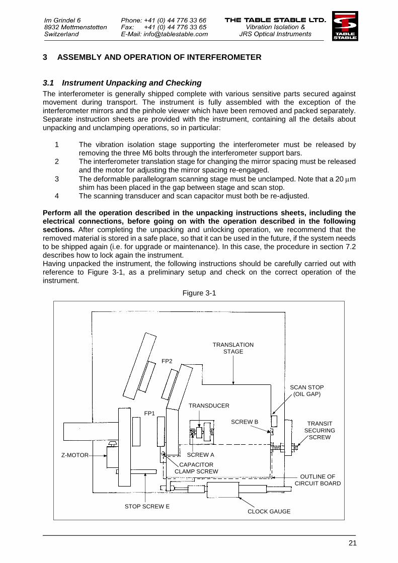
4 The scanning transducer and scan capacitor must both be re-adjusted. Perform all the operation described in the unpacking instructions sheets, including the electrical connections, before going on with the operation described in the following sections. After completing the unpacking and unlocking operation, we recommend that the removed material is stored in a safe place, so that it can be used in the future, if the system needs to be shipped again (i.e. for upgrade or maintenance). In this case, the procedure in section 7.2 describes how to lock again the instrument. Having unpacked the instrument, the following instructions should be carefully carried out with reference to Figure 3-1, as a preliminary setup and check on the correct operation of the instrument.

Figure 3-1

FP1

FP2

TRANSLATIONSTAGE

SCREW B

SCAN STOP(OIL GAP)

TRANSIT

SECURINGSCREW

OUTLINE OFCIRCUIT BOARD

CLOCK GAUGESTOP SCREW E

CAPACITORCLAMP SCREW

TRANSDUCER

SCREW AZ-MOTOR

22

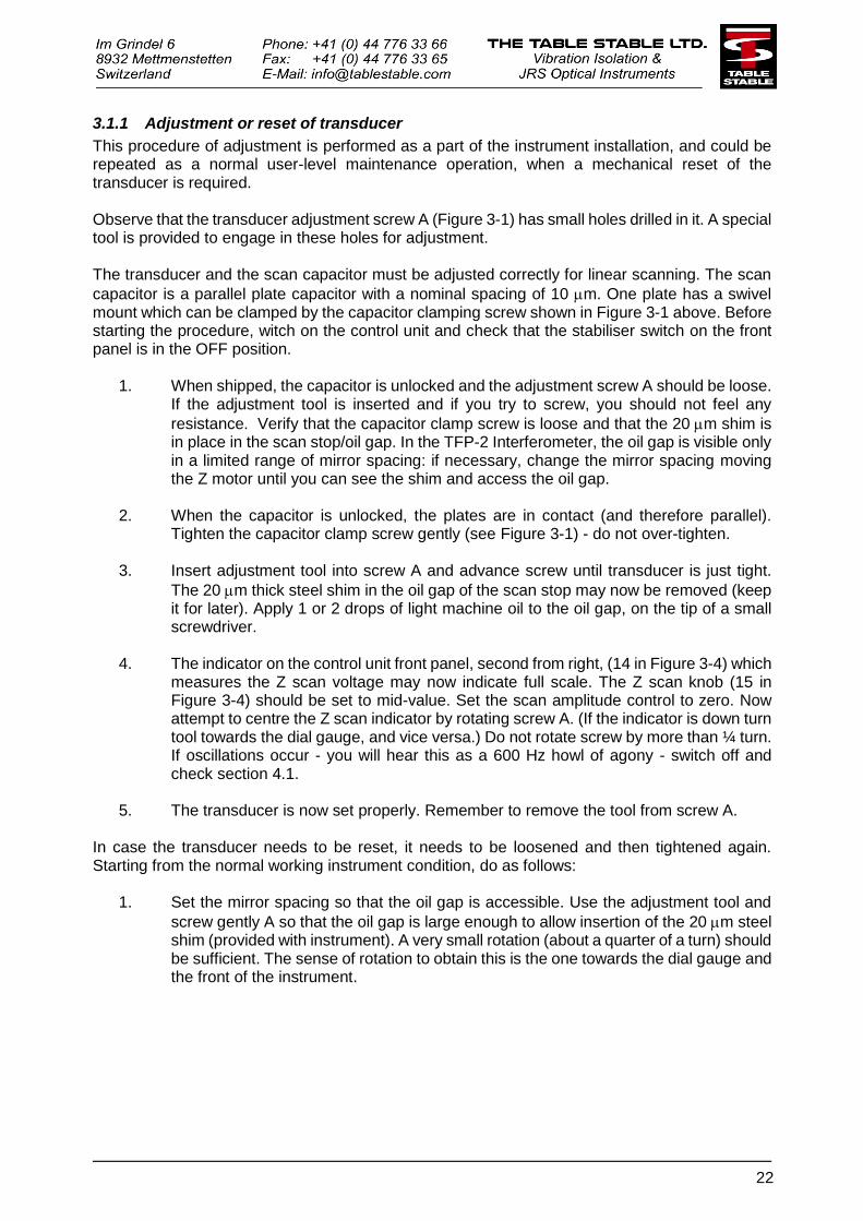
3.1.1 Adjustment or reset of transducer

This procedure of adjustment is performed as a part of the instrument installation, and could be repeated as a normal user-level maintenance operation, when a mechanical reset of the transducer is required. Observe that the transducer adjustment screw A (Figure 3-1) has small holes drilled in it. A special tool is provided to engage in these holes for adjustment. The transducer and the scan capacitor must be adjusted correctly for linear scanning. The scan

capacitor is a parallel plate capacitor with a nominal spacing of 10 m. One plate has a swivel mount which can be clamped by the capacitor clamping screw shown in Figure 3-1 above. Before starting the procedure, witch on the control unit and check that the stabiliser switch on the front panel is in the OFF position.

1. When shipped, the capacitor is unlocked and the adjustment screw A should be loose. If the adjustment tool is inserted and if you try to screw, you should not feel any

resistance. Verify that the capacitor clamp screw is loose and that the 20 m shim is in place in the scan stop/oil gap. In the TFP-2 Interferometer, the oil gap is visible only in a limited range of mirror spacing: if necessary, change the mirror spacing moving the Z motor until you can see the shim and access the oil gap.

2. When the capacitor is unlocked, the plates are in contact (and therefore parallel). Tighten the capacitor clamp screw gently (see Figure 3-1) - do not over-tighten.

3. Insert adjustment tool into screw A and advance screw until transducer is just tight.

The 20 m thick steel shim in the oil gap of the scan stop may now be removed (keep it for later). Apply 1 or 2 drops of light machine oil to the oil gap, on the tip of a small screwdriver.

4. The indicator on the control unit front panel, second from right, (14 in Figure 3-4) which

measures the Z scan voltage may now indicate full scale. The Z scan knob (15 in Figure 3-4) should be set to mid-value. Set the scan amplitude control to zero. Now attempt to centre the Z scan indicator by rotating screw A. (If the indicator is down turn tool towards the dial gauge, and vice versa.) Do not rotate screw by more than ¼ turn. If oscillations occur - you will hear this as a 600 Hz howl of agony - switch off and check section 4.1.

5. The transducer is now set properly. Remember to remove the tool from screw A.

In case the transducer needs to be reset, it needs to be loosened and then tightened again. Starting from the normal working instrument condition, do as follows:

1. Set the mirror spacing so that the oil gap is accessible. Use the adjustment tool and

screw gently A so that the oil gap is large enough to allow insertion of the 20 m steel shim (provided with instrument). A very small rotation (about a quarter of a turn) should be sufficient. The sense of rotation to obtain this is the one towards the dial gauge and the front of the instrument.

23

2. Using a pair of small tweezers, pass the steel shim through the oil gap of the scan stop in order to clean it. Finally leave the shim in the gap. After this, unscrew the transducer screw A by moving the tool toward the back of the instrument, until the parallelogram will rest on the shim. At that point, the adjustment tool will lose tension will tend to fall on the stage, there is no harm if this happens.

3. Slacken the transducer adjustment screw A. As soon as this screw is slackened the transducer will be loose and the spring around screw B will cause the scanning stage to move against the scan stop.

4. Slacken the capacitance clamp screw. This automatically brings the capacitance

plates into contact. Tighten capacitance clamp screw again being careful not to apply a lot of force.

5. At this point the previous procedure can be repeated starting from step 3 and the

mechanical adjustment of the scanning stage will then be complete

3.1.2 Further check of control unit

1. Rotate the Z scan knob between extreme positions - the Z scan indicator should vary over

about plus/minus one division of the scale. (The stabiliser switch must be in OFF position!) 2. Increase scan amplitude control from zero and observe appropriate movement of the Z scan

indicator.

3. Observe that movement of the adjustment potentiometers for X1, Y1, Z, X2 and Y2 cause movements of the appropriate indicators over the full scale.

After an initial settling period, or when significant variations of temperature have occurred, it may be necessary to repeat the transducer adjustment, as described in the previous paragraph 3.1.1, step 4: the adjustment screw A can be rotated by a small angle in order to bring the scan amplitude LED indicator to midrange. If this is not sufficient, the transducer reset procedure can be performed (end of paragraph 3.1.1). The translation stage may be moved by using the Z-motor control on the spectrometer housing. Observe the mirror spacing indicated by the dial gauge. Note also the STOP screw E which prevents the mirrors from being brought too close together (don’t be afraid – nothing will happen if they do touch).

CAUTION The electronics board on the translation stage has 200 V present on some components and conductors. Take care that no grounded metal objects or fingers come into contact with this board, for example when adjusting transducer.

24

3.2 Operation of Isolation System

When operating the system for the first time, set the front panel isolation switch to OFF and switch on power. The green LED will light (indicating power) and all the output saturation warning lights will illuminate. After a few seconds these warning lights will begin to go out or flicker. It may take about 15 seconds for the last ones to go out. After 30 seconds switch the isolation switch to ON and the yellow LED will glow indicating that the system is stabilising. During normal operation all warning lights should be out. Excessive forces applied to the interferometer will cause input and/or output circuits to saturate - this makes a useful check that all isolation elements are working. A severe overload causes the system to switch off for a few moments before attempting to stabilise again. In the normal course of events the front panel isolation switch may be left ON and the system switched on and off using the power switch. After switching on there is a built-in delay of about 20 seconds before the system isolates. During this period the isolation indication lamp blinks. The system will be operating correctly when all overload indicator lamps are out and the isolation indicator lamp is on. Note The rear panel BNC socket gives a multiplexed output showing the signals from all 8 accelerometers. These signals can be viewed on a simple analogue oscilloscope by setting the time base to 20ms and sensitivity to 0.5V. On setting up for the first time it is strongly recommended that you look at this signal, with the isolation switch both ON and OFF - it gives a good impression of how well the system is operating. Pushing sideways on your optical table should NOT cause any of the LEDs to light up. If they do, the support legs of your table are not rigid enough.

25

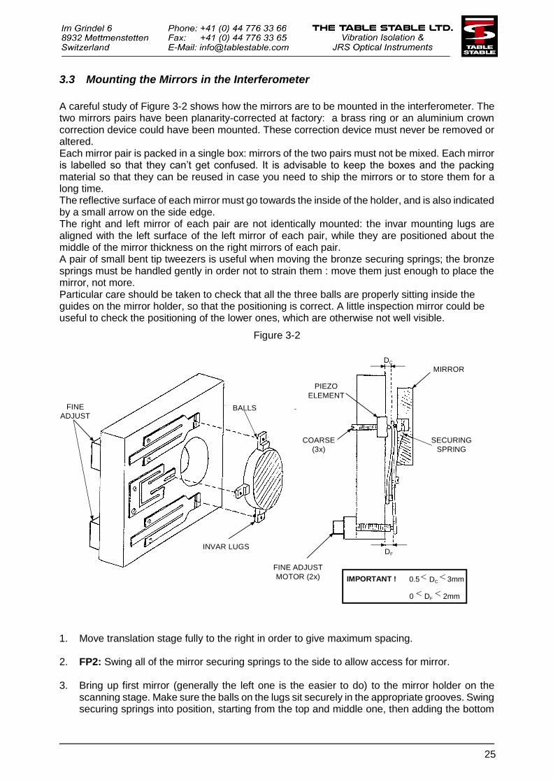
3.3 Mounting the Mirrors in the Interferometer

A careful study of Figure 3-2 shows how the mirrors are to be mounted in the interferometer. The two mirrors pairs have been planarity-corrected at factory: a brass ring or an aluminium crown correction device could have been mounted. These correction device must never be removed or altered. Each mirror pair is packed in a single box: mirrors of the two pairs must not be mixed. Each mirror is labelled so that they can’t get confused. It is advisable to keep the boxes and the packing material so that they can be reused in case you need to ship the mirrors or to store them for a long time. The reflective surface of each mirror must go towards the inside of the holder, and is also indicated by a small arrow on the side edge. The right and left mirror of each pair are not identically mounted: the invar mounting lugs are aligned with the left surface of the left mirror of each pair, while they are positioned about the middle of the mirror thickness on the right mirrors of each pair. A pair of small bent tip tweezers is useful when moving the bronze securing springs; the bronze springs must be handled gently in order not to strain them : move them just enough to place the mirror, not more. Particular care should be taken to check that all the three balls are properly sitting inside the guides on the mirror holder, so that the positioning is correct. A little inspection mirror could be useful to check the positioning of the lower ones, which are otherwise not well visible.

Figure 3-2

INVAR LUGS

PIEZO

ELEMENT

COARSE

(3x)

SECURING

SPRING

MIRROR

DC

FINE ADJUST

MOTOR (2x)

BALLSFINE

ADJUST

DF

IMPORTANT !

DF

DC0.5 3mm

0 2mm

1. Move translation stage fully to the right in order to give maximum spacing. 2. FP2: Swing all of the mirror securing springs to the side to allow access for mirror. 3. Bring up first mirror (generally the left one is the easier to do) to the mirror holder on the

scanning stage. Make sure the balls on the lugs sit securely in the appropriate grooves. Swing securing springs into position, starting from the top and middle one, then adding the bottom

26

one. After moving all the spring in position, use the inspection mirror for a further check of the balls positions.

4. Repeat the operation with second mirror to be mounted on the mirror holder. 5. FP1: Before mounting the scanning mirror of FP1 move the spring that will hold the middle

lug to the left so that it lies on top of the corresponding lug of FP2. 6. Mount mirrors of FP1 as in (1) to (4) above. The exact relative spacing of FP1 and FP2 will be obtained later when calibrating mirror spacing.

27

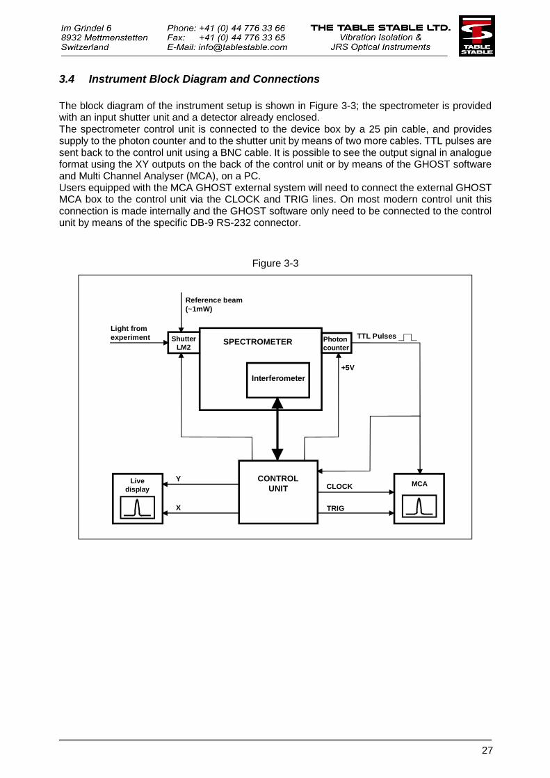
3.4 Instrument Block Diagram and Connections

The block diagram of the instrument setup is shown in Figure 3-3; the spectrometer is provided with an input shutter unit and a detector already enclosed. The spectrometer control unit is connected to the device box by a 25 pin cable, and provides supply to the photon counter and to the shutter unit by means of two more cables. TTL pulses are sent back to the control unit using a BNC cable. It is possible to see the output signal in analogue format using the XY outputs on the back of the control unit or by means of the GHOST software and Multi Channel Analyser (MCA), on a PC. Users equipped with the MCA GHOST external system will need to connect the external GHOST MCA box to the control unit via the CLOCK and TRIG lines. On most modern control unit this connection is made internally and the GHOST software only need to be connected to the control unit by means of the specific DB-9 RS-232 connector.

Figure 3-3

SPECTROMETER

Interferometer

Shutter

LM2

Live

displayMCA

TRIG

Y

X

Reference beam

(~1mW)

Light from

experiment Photon

counter

CLOCKCONTROL

UNIT

TTL Pulses

+5V

28

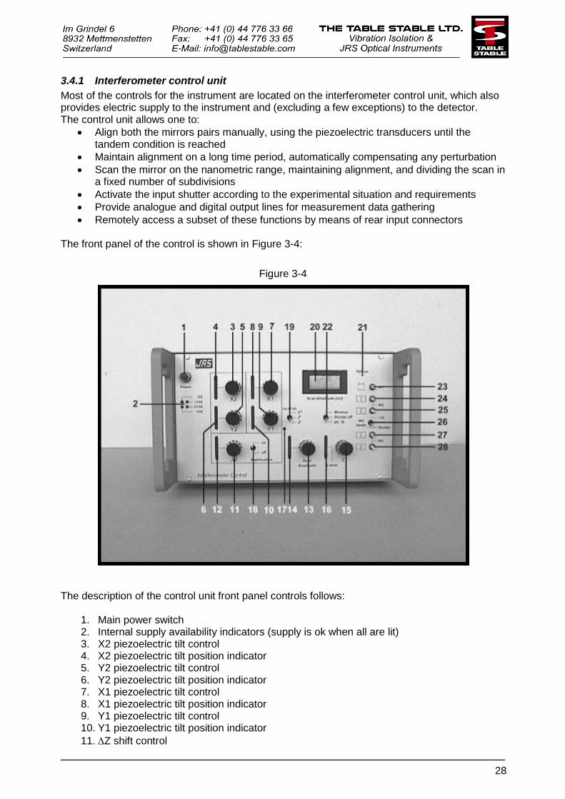
3.4.1 Interferometer control unit

Most of the controls for the instrument are located on the interferometer control unit, which also provides electric supply to the instrument and (excluding a few exceptions) to the detector. The control unit allows one to:

Align both the mirrors pairs manually, using the piezoelectric transducers until the tandem condition is reached

Maintain alignment on a long time period, automatically compensating any perturbation

Scan the mirror on the nanometric range, maintaining alignment, and dividing the scan in a fixed number of subdivisions

Activate the input shutter according to the experimental situation and requirements

Provide analogue and digital output lines for measurement data gathering

Remotely access a subset of these functions by means of rear input connectors The front panel of the control is shown in Figure 3-4:

Figure 3-4

The description of the control unit front panel controls follows:

1. Main power switch 2. Internal supply availability indicators (supply is ok when all are lit) 3. X2 piezoelectric tilt control 4. X2 piezoelectric tilt position indicator 5. Y2 piezoelectric tilt control 6. Y2 piezoelectric tilt position indicator 7. X1 piezoelectric tilt control 8. X1 piezoelectric tilt position indicator 9. Y1 piezoelectric tilt control 10. Y1 piezoelectric tilt position indicator

11. Z shift control

29

12. Z shift position indicator 13. Scan amplitude control 14. Scan position indicator 15. Z shift control 16. Z shift position indicator 17. Scan amplitude LCD display indicator calibration screw 18. Stabiliser feedback switch 19. Number of channel selector 20. Scan amplitude LCD display indicator 21. Detector supply indicator LED 22. Shutter mode selector 23. Main shutter window width control 24. Secondary shutter window start position control 25. Secondary shutter window width control 26. Secondary shutter window mode selector 27. Tertiary shutter window start position control 28. Tertiary shutter window width control

The meaning of many of these controls may be immediately clear to the reader; the main functions of the control unit will be described in detail in this chapter. The LED indicator 21 on the front panel shows the position of the switch on the rear panel of the control unit. It is important to note that it will be meaningful only when the instrument detector is powered through the control unit: if your detector is powered by means of a separate power supply, the LED information will have no relationship with the status of the detector.

30

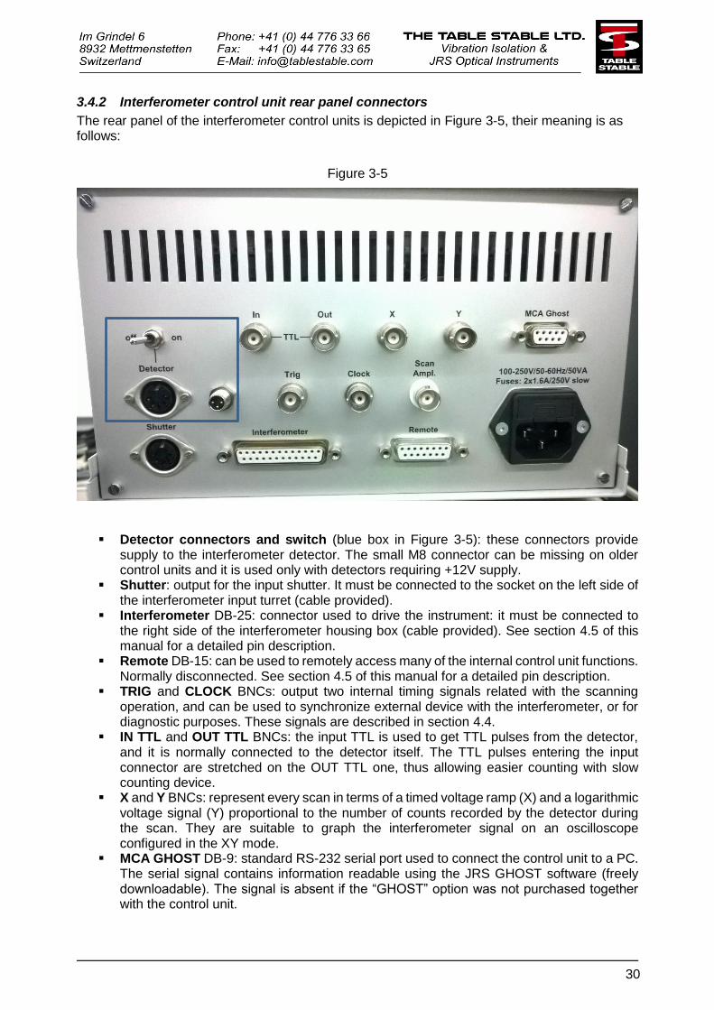
3.4.2 Interferometer control unit rear panel connectors

The rear panel of the interferometer control units is depicted in Figure 3-5, their meaning is as follows:

Figure 3-5

Detector connectors and switch (blue box in Figure 3-5): these connectors provide supply to the interferometer detector. The small M8 connector can be missing on older control units and it is used only with detectors requiring +12V supply.

Shutter: output for the input shutter. It must be connected to the socket on the left side of the interferometer input turret (cable provided).

Interferometer DB-25: connector used to drive the instrument: it must be connected to the right side of the interferometer housing box (cable provided). See section 4.5 of this manual for a detailed pin description.

Remote DB-15: can be used to remotely access many of the internal control unit functions. Normally disconnected. See section 4.5 of this manual for a detailed pin description.

TRIG and CLOCK BNCs: output two internal timing signals related with the scanning operation, and can be used to synchronize external device with the interferometer, or for diagnostic purposes. These signals are described in section 4.4.

IN TTL and OUT TTL BNCs: the input TTL is used to get TTL pulses from the detector, and it is normally connected to the detector itself. The TTL pulses entering the input connector are stretched on the OUT TTL one, thus allowing easier counting with slow counting device.

X and Y BNCs: represent every scan in terms of a timed voltage ramp (X) and a logarithmic voltage signal (Y) proportional to the number of counts recorded by the detector during the scan. They are suitable to graph the interferometer signal on an oscilloscope configured in the XY mode.

MCA GHOST DB-9: standard RS-232 serial port used to connect the control unit to a PC. The serial signal contains information readable using the JRS GHOST software (freely downloadable). The signal is absent if the “GHOST” option was not purchased together with the control unit.

31

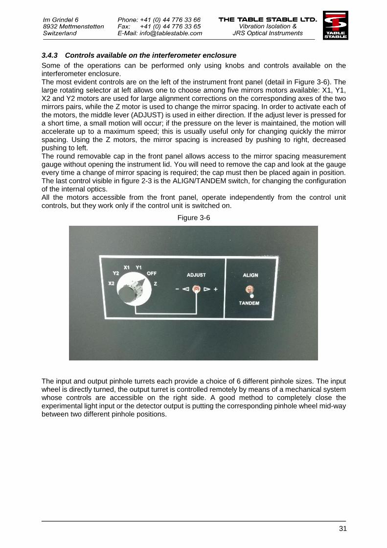
3.4.3 Controls available on the interferometer enclosure

Some of the operations can be performed only using knobs and controls available on the interferometer enclosure. The most evident controls are on the left of the instrument front panel (detail in Figure 3-6). The large rotating selector at left allows one to choose among five mirrors motors available: X1, Y1, X2 and Y2 motors are used for large alignment corrections on the corresponding axes of the two mirrors pairs, while the Z motor is used to change the mirror spacing. In order to activate each of the motors, the middle lever (ADJUST) is used in either direction. If the adjust lever is pressed for a short time, a small motion will occur; if the pressure on the lever is maintained, the motion will accelerate up to a maximum speed; this is usually useful only for changing quickly the mirror spacing. Using the Z motors, the mirror spacing is increased by pushing to right, decreased pushing to left. The round removable cap in the front panel allows access to the mirror spacing measurement gauge without opening the instrument lid. You will need to remove the cap and look at the gauge every time a change of mirror spacing is required; the cap must then be placed again in position. The last control visible in figure 2-3 is the ALIGN/TANDEM switch, for changing the configuration of the internal optics. All the motors accessible from the front panel, operate independently from the control unit controls, but they work only if the control unit is switched on.

Figure 3-6

The input and output pinhole turrets each provide a choice of 6 different pinhole sizes. The input wheel is directly turned, the output turret is controlled remotely by means of a mechanical system whose controls are accessible on the right side. A good method to completely close the experimental light input or the detector output is putting the corresponding pinhole wheel mid-way between two different pinhole positions.

32

3.4.4 Familiarizing yourself with the tandem interferometer

Once the interferometer has been installed it is a good idea to send light into the spectrometer and follow the course of the beam through the system. In order to do this the interferometer has to be aligned and so you will learn the functions of the different alignment controls. Before starting make sure that the photomultiplier is switched off and stays switched off (switch on the back of the control unit). Switch on the control unit and switch the shutter switch (22) to the OFF position. This will open the entrance shutter. The best way to put light into the spectrometer is to place a 10mm focal length lens in front of the entrance pinhole and adjust the position and focus of the lens until the light passes cleanly through the pinhole and fills the aperture A1. Refer to Figure 2-3 and Figure 2-4 in order to identify the various optical components. Do not be tempted to adjust any of the optics inside the spectrometer enclosure – to do so is guaranteed to cause some misalignment! 1. Remove the lid from the spectrometer housing and remove the internal black protection

screens too. Information on how to do this are provided in section 7.2, part 6.

2. With the lid removed from the spectrometer, take a small piece of paper and follow the light beam from A1 onto M1 and thence through lens L1 where the beam is collimated. On the front panel of the spectrometer is a switch for changing the optics system from the alignment to the tandem mode – switch from one position to the other and observe the movement. The stage must be allowed to run to the limit before switching back. Finally leave the system in the Tandem mode.

3. On the control unit set the scan amplitude (13) to zero. Hold a piece of paper just after FP1

and adjust Z (15) so that FP1 transmits. You should see a fringe, more or less sharp, depending on the degree of alignment. Try adjusting Y1 (8) from limit to limit, at the same time making small adjustments to Z to keep the fringe in view. At the limits of Y1 the fringe will sharpen and become horizontal. Adjust Y1 until the fringe becomes as broad as possible – at this point the fringe will have rotated through 90° until it is vertical. Now use the X1 adjustment (7) to make the fringe so broad that it fills the aperture. You may have to return to Y1 to optimize. Finally check the third pass through FP1 and optimise again.

4. Repeat the above procedure until you can easily and quickly align FP1. This is best done as

a two-handed operation – one hand on Z and the other on X1 or Y1. When the fringe is as broad as possible try making a small modulation with Z. If the fringe is optimally adjusted it should flash at you, if the alignment is not yet perfect the fringe will be displaced as it flashes. Avoid breathing on the interferometer when making this alignment because it reacts very sensitively to the slightest temperature change. You should also switch off your air conditioning if it is causing a lot of air movement.

5. Now try to adjust FP2 following the same procedure. The whole time you must make sure

that FP1 transmits otherwise you will have no light to pass through FP2! Place the piece of

paper after FP2 and use X2 and Y2 to prealign FP2. It will be necessary to adjust Z to keep

the fringe in view. Optimise the transmission using X2, Y2 and Z. Finally check the third pass through FP2 and optimise. The interferometer is now fully aligned.

33

6. If the photon detector has been removed, you can now follow the beam through the output pinhole.

7. The path of the alignment beam can be followed by switching the optics to the alignment mode. Place the paper between BS1 and BS2. Make a manual scan by turning Z – you should see a black fringe moving across the paper. When FP1 is fully aligned the fringe fills the aperture and the beam becomes dark. Notice that the dark field is not completely black, partly because the intensity of the black fringe is not exactly zero and partly due to the non-linear response of the eye.

8. If you now place the paper after FP2 you will see the same fringe, and if you continue to

adjust Z you will then see a fringe due to FP2. These fringes will normally be easily distinguishable as you scan Z due to the differing degrees of alignment of the two interferometers.

9. If you stop the Z movement when the fringe from FP1 is in view, you can then adjust Z to bring the fringe from FP2 to overlap. This shows the principle of the alignment mode – in practice this alignment is done in the scanning mode as discussed below.

3.4.5 Use of the detector and of the MCA GHOST data gathering system

The alignment of the internal components is most easily assessed using a strong beam of light either coming directly from the laser source or obtained focussing a laser sport on an unpolished metallic surface. When doing this, the device detector is always switched off (and/or the output pinhole wheel put in the middle between two positions) in order to avoid any possibility of damaging the light sensitive element. Most of the routine operations and several instrument checks can be also performed in the normal operating condition, i.e. using the reference beam as a source and the instrument detector. In these cases, the input pinhole will be normally kept closed (in the middle between two positions) and the instrument lid will be closed too. The signal can be seen through the X, Y and OUT connectors or through the DB-9 RS-232 (serial port) output on the rear panel on the control unit. The GHOST MultiChannel Analyser (MCA) is a software and hardware system which allows to output information using the serial output and represent them on a personal computer. The GHOST hardware system is available as an optional component of the control unit, the software is available free of charge. For a detailed explanation of the functions of the GHOST application, we direct the reader to the related manual, included in the spectrometer’s documentation. In some of the following sections, the MCA software (observation mode) will be used to monitor the spectrometer output while scanning the mirror spacing in the alignment mode spectrometer configuration. When in alignment mode, the GHOST software will evidence the dips produced by

the mirror transmission, when the spacing of each FP is an integer multiple of /2. The intensity of the signal in alignment mode can be trimmed by changing the alignment beam position with respect to the reference input.

3.4.6 Changing the mirror spacing

Depending on the resolution required it will be necessary to change the interferometer mirror spacing. Ensure the stabiliser is off and switch the optics to the alignment mode. The dips related to the two FP pairs should be seen on the GHOST MCA. It does not matter if they are not quite optimized. Proceed as follows: 1. Turn the axis-switch on the front panel of the spectrometer housing to Z. With the adjacent

switch a movement to the left or right will decrease or increase the spacing respectively.

34

Follow the spacing change on the dial gauge and at first do not change the spacing by more than 1 mm. You should still be able to see the dips in the signal but they will not be so sharp. Optimize using the X1, Y1 and X2, Y2 controls. Change by a further 1 mm as above until the required spacing has been reached.

2. Having optimized the alignment dips check the voltages displayed for X1, Y1 and X2, Y2. For

good long term stability these voltages should not lie too near to the extremes. If any of these signals is out of range, proceed to the next section.

3. If the signals are all within range use Z to bring two dips near the centre into coincidence. Use the Z adjustment to bring the coincident dips to the scan centre.

4. Switch the optics back to the tandem mode and optimize the alignment. 5. Switch on the stabilisers.

The procedure for alignment and scanning is also described in a more detailed way in section 0.

3.4.7 Motor compensation of PZT drift

In the event that one or more of the voltages X1, Y1 and X2, Y2 displayed on the control unit are out of range, they may be readjusted using the motor controls. The control panel on the spectrometer housing allows fine motor control of the above axes. For example to correct X2, first of all use the X2 adjustment on the control unit to return the voltage towards mid-range, making sure that the corresponding dip for FP2 is still visible. Now turn the axis-select switch on the control panel to X2 and use the adjacent switch (the same one you used for the spacing change) to optimize the dips. Do not hold the switch for more than a second because the correction begins to speed up and you may end up completely misaligning the axis. Use repetitive short corrections. You cannot optimize perfectly using the motor controls so return to the control unit and optimize using the X2 and Y2 adjustments. If the voltage for X2 is still not near enough to the centre repeat the procedure. Repeat for any further axes.

3.4.8 Learning to use the scan control

In most Brillouin scattering experiments it is essential to be able to modulate the laser intensity reaching the photomultiplier. Thus in back-scattering experiments there is often so much elastic light that the photon counting system is saturated and so no signal is available for stabilising the interferometer. In this case it is necessary to reduce the laser intensity while scanning through the elastic peak. In 90° or forward scattering experiments there is often so little light that the photon counting system offers insufficient signal for stabilising. In this case it is necessary to introduce some extra laser light into the scattered light signal. This extra signal is not always desirable - for example when studying central modes. Here the only solution is to separate the stabilisation cycles from the measurement cycles - for example by introducing extra laser light only during a cycle of 16 stabilisation scans (MCA gated off) followed by 16 scans when the signal alone is recorded.

35

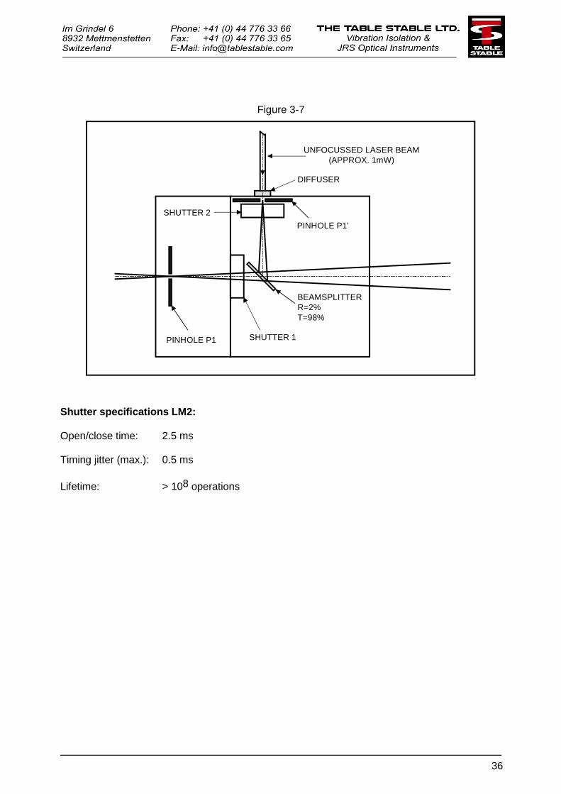
A double shutter system is integrated into the optical system directly behind the entrance pinhole to the spectrometer. This allows all of the above experimental situations to be easily addressed. The device operates in conjunction with a reference beam as follows (refer also to the input turret diagram in Figure 3-7): a) For scattering experiments where the elastic signal is too strong, a signal is sent from the

control unit to close the shutter 1 while scanning through the elastic peak, and a suitable reference signal is introduced for stabilisation purposes via the secondary pinhole with shutter 2 open.

b) For scattering experiments where insufficient elastic signal is available for stabilisation

purposes, the situation is similar to the above case except that shutter 1 and 2 both remain permanently open.

c) If the extra light signal from the secondary pinhole disturbs the measurement, then shutter 2

is opened for a cycle of 16 stabilisation scans while the MCA TRIG signal is gated off. During the next 16 scans shutter 2 is closed and the experimental signal is recorded. The cycle repeats.

In order to operate the shutter a trigger signal is required. This is known as a "window” signal and is generated in the control unit as described in the next section.

36

Figure 3-7

UNFOCUSSED LASER BEAM

(APPROX. 1mW)

DIFFUSER

PINHOLE P1'

PINHOLE P1 SHUTTER 1

SHUTTER 2

BEAMSPLITTER

R=2%

T=98%

Shutter specifications LM2: Open/close time: 2.5 ms Timing jitter (max.): 0.5 ms

Lifetime: > 108 operations

37

3.4.9 Window operation

Referring to Figure 3-4, set the front panel switch (22) to "window" and the mode switch (26) to shutter. The shutters are controlled by the 3 windows W1 - W3. Outside of these windows shutter 1 is open and shutter 2 closed. The transmission through the beam splitter is about 98% so there is no serious loss of signal. Within any of the windows shutter 1 closes and shutter 2 opens, allowing the reference beam (consisting of about 0.5 mW of unfocussed laser light falling on the diffuser outside pinhole P1') to pass through the spectrometer. This is the simplest mode of operation. The windows can be simply adjusted as described below. Adjustment of Windows The position of the windows is shown at the bottom of the Spectrum Display signal available at the X and Y outputs at the rear of the control unit (or by a colour change in the GHOST software). The central window cannot be turned off. The width is adjusted by potentiometer (23). The width of the second window pair W2 is determined by (25) and if not required can be adjusted to zero. The position of the window is adjusted by potentiometer (24) If required a third window pair W3 may be set using potentiometers (27) and (28). Alt.16 Special Shutter mode, for Measurement without an Elastic Peak For measurements having no intrinsic elastic peak and where it is desirable to measure right through the central portion of the spectrum, it is possible to separate the stabilisation cycles from the measurement cycles so that the reference signal does not appear as part of the spectrum. Switch the shutter switch (20) to "alt. 16". For a period of 16 scans shutter 1 is closed and the interferometer stabilises on the light signal falling on P1'. During this period the MCA TRIG signal is disabled so that no signal is recorded by the MCA. For the next 16 scans shutter 1 opens and shutter 2 closes, TRIG is enabled and the spectrum is recorded even in the complete absence of an elastic peak. ÷10 Special Shutter mode, to Enhance Weak Spectral Features The function of the window W2 can be changed to enable parts of the spectrum to be selectively scanned at a slower rate thus allowing weak signals to be seen more quickly. Set the window W2 to the desired part of the spectrum as above and switch the mode switch (26)

to "10": the channels covered by W2 will have a 10 times longer duration.

38

3.4.10 Scanning the Tandem Interferometer

In order to learn more about the operation of the spectrometer it is necessary to scan the instrument and measure the transmitted signal using the photon detector. This can conveniently be done using the reference beam via the shutter unit. Scanning is normally monitored through the GHOST software application or by means of third party hardware and software bundles. The following procedure describes how to operate the control unit for a basic scanning and use the XY output BNC connectors on the rear panel of the control unit in order to observe the interferometer signal. The same signal will be digitally represented using the GHOST application. The procedure can be equivalently performed using GHOST instead of the XY output ports; in this case the point 1 below can be omitted. It is quite difficult to observe the slow scan on an oscilloscope. We strongly recommend that you observe the signal using the GHOST multichannel analyser software. This software refreshes the displayed signal each scan and is much easier on the eyes! 1 Connect the detector to the TTL input on the rear panel of the control unit. The signal can be

viewed in the X-Y mode on an oscilloscope. Connect the X-output signal from the rear of the control unit to the X-input of an oscilloscope with a sensitivity of 0.5 V per division. Connect the Y-output signal from the control unit to the Y-input of the oscilloscope with a sensitivity of 1 V per division. You will observe there is a baseline to the spectrum with a small square wave marker in the centre (there may be other markers but you can ignore these for the moment).

2 With the optics switched to the alignment mode, adjust the light intensity until a signal of

about 2 V is seen on the oscilloscope. This corresponds to a count rate of about 300 kcts/s, or 300 counts/channel when using 512 channels mode. It is easy to observe the changes in intensity (due to the different time spent on each channel) when changing from 512 channels to 1024 or 256, and back.

3 Turn the scan amplitude knob until a reading of about 600 nm is seen on the LCD display.

The Y-signal should now show two series of three dips. Change Z and observe that only one of these series moves – the dips that move correspond to FP2. Adjust X2 and Y2 to make the dips as deep as possible. The display is logarithmic so the dips will not go completely to zero. FP2 is now adjusted.

4 Repeat for X1 and Y1 and again make the dips as deep as possible. FP1 is now also aligned.

5 Adjust Z so as to bring two dips near the centre of the scan together. Notice that by adjusting Z all the peaks move together. The axis Z can be used to bring the coincident dips to the centre of the scan, i.e. to the centre of the marker.

6 The interferometer is now prealigned. Switch the optics to the Tandem mode and you should

see a single peak in the centre of the scan. By successively adjusting all axes maximize the height of this peak. If you have done everything correctly, the peak height should be at least 1V higher than the alignment mode intensity (corresponding to a factor of 3 or more in intensity).

7 You can now switch on the stabiliser (18). The peak should move to the exact scan centre

and after a few scans reach maximum amplitude. The stabilisers should hold this alignment

indefinitely provided the room temperature does not change by more than 2C.

39

Note The stabilisers will only work if the peak was placed within the marker before switching on. Observe the Z-error display. This is a dual display showing both the Z-correction signal and also the drift of the peak from the scan centre. The longer flash shows the Z-correction signal, the shorter one the peak drift. Once the stabiliser has been switched on for a few scans the latter should be in the centre of the display. Of course if the Z-correction also happens to be zero the two signals will be coincident and so the display will not flash.

40

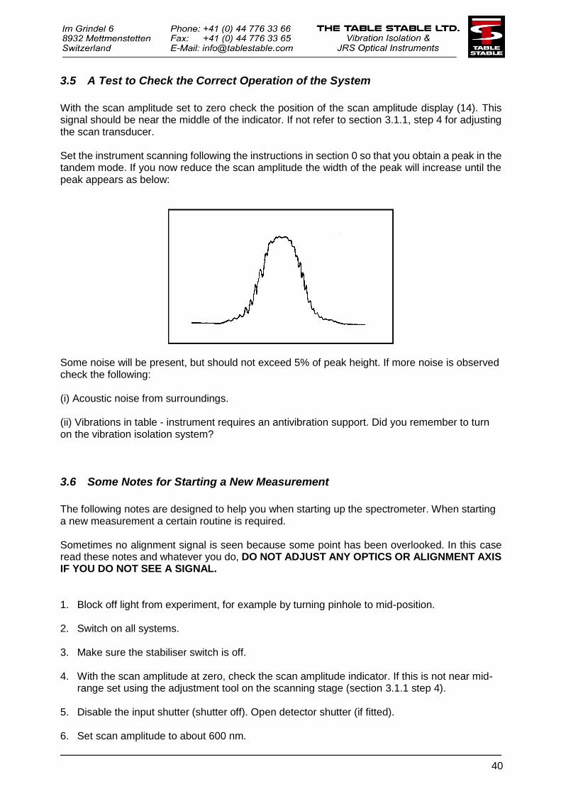
3.5 A Test to Check the Correct Operation of the System

With the scan amplitude set to zero check the position of the scan amplitude display (14). This signal should be near the middle of the indicator. If not refer to section 3.1.1, step 4 for adjusting the scan transducer. Set the instrument scanning following the instructions in section 0 so that you obtain a peak in the tandem mode. If you now reduce the scan amplitude the width of the peak will increase until the peak appears as below:

Some noise will be present, but should not exceed 5% of peak height. If more noise is observed check the following: (i) Acoustic noise from surroundings. (ii) Vibrations in table - instrument requires an antivibration support. Did you remember to turn on the vibration isolation system?

3.6 Some Notes for Starting a New Measurement

The following notes are designed to help you when starting up the spectrometer. When starting a new measurement a certain routine is required. Sometimes no alignment signal is seen because some point has been overlooked. In this case read these notes and whatever you do, DO NOT ADJUST ANY OPTICS OR ALIGNMENT AXIS IF YOU DO NOT SEE A SIGNAL. 1. Block off light from experiment, for example by turning pinhole to mid-position. 2. Switch on all systems. 3. Make sure the stabiliser switch is off. 4. With the scan amplitude at zero, check the scan amplitude indicator. If this is not near mid-

range set using the adjustment tool on the scanning stage (section 3.1.1 step 4). 5. Disable the input shutter (shutter off). Open detector shutter (if fitted). 6. Set scan amplitude to about 600 nm.

41

7. Switch the optics to the alignment mode and adjust the reference intensity to give a signal of

about 2 – 3V on the oscilloscope display. If you are observing the signal on the MCA GHOST, adjust the signal intensity for about 200’000 to 300’000 cts/s (corresponding to 100 to 150 cts per scan with 1024 channels). If you see no reference signal STOP AND THINK – do not adjust anything!

8. Adjust Z and Z displays to about mid-range.

9. Optimize alignment signal and synchronize a dip from FP1 and one from FP2 using Z. Place in the centre of the scan using Z.

10. Switch optics to the tandem mode and optimize. Note that the signal should be in the range

between 3 and 5 times higher than in the alignment mode (corresponding to about 1 V higher on the logarithmic oscilloscope display). Move the signal to within the central window.

11. If necessary readjust the reference intensity to avoid saturation of the display signal on the

oscilloscope. 12. Switch the stabiliser ON. 13. Set the required window (usually just W1) and switch on shutter. 14. Return input pinhole to correct position. Output pinhole should be one stop larger (or

approximately 1.5 times in diameter). 15. Start the measurement.

3.7 Photon Counting Limit, Detector Linearity and Saturation

During operation, the instrument control unit will provide as output the number of counts read by the interferometer detector and, in turn, the intensity of light at a certain frequency shift with respect to the reference beam. The number of counts for each channel is limited by electronics and detector capabilities. In order to avoid distortions in the spectrum, the user must take care that the reference beam and the experimental light are both in the acceptable intensity region. The number of counts is hardware limited mainly by two factors:

The range of the digital counter inside the control unit circuitry: a 12 bit counter is used, so up to 212 = 4096 photons can be counted for each channel before a counter roll-off occurs. When the intensity of signal produces enough counts to go over this limit, the counter resets and the excess count number is recorded: in a peak, this will lead to very strong apparent changes in the intensity. It will be easy to reach this limit in the reference beam when its intensity is too high.

The saturation and linearity limits of the installed detector, which are usually provided by the original manufacturer in terms of counts/s, and together with linearity correction formulas when available. These effects may be more subtle and vary from a detector to another. A detailed calibration sheet for the detector is supplied by the detector manufacturer and will provide information of the saturation limit and linearity behaviour for the detector mounted in your instrument.

The number of counts at which the instrument will approach detector saturation and nonlinear behaviour also depends by the number of channels selected in the control unit: using 1024 channels, the time spent on each channel is 0.5ms, at 512 channels, it is 1ms and at 256 channels it is 2ms.

42

The TFP-2 HC interferometer is provided at present with two different detectors: the Laser Components COUNT® Blue SAPD detector and the Hamamatsu H10682 photomultiplier module. In both cases, the detector starts to have a noticeably nonlinear behaviour in the range of 3·106 counts/s. This means that you can see nonlinearity and then saturation effects in the range of 1500 counts per channel when working with a 1024 channels configuration, or 3000 counts per channel when working with a 512 channels configuration. Using the Hamamatsu module, which has about 10% quantum efficiency, it is quite difficult to have such a big intensity in an experimental signal of interest and care should be taken only concerning the intensity of reference light as seen in the alignment mode. When using the SAPD detector, which is much more sensitive, it is actually possible to produce Brillouin peaks whose intensity is approaching the nonlinear region. In this case, the intensity of the experimental laser beam could be reduced until the linearity correction is expected to be negligible, or otherwise an intensity correction could be mathematically applied. Refer to the detectors datasheets for useful linearity correction formulas.

3.8 Polarisation Selectivity in the TFP-2 HC

The use of polarisation optics inside the high contrast interferometer TFP-2 brings as a consequence that the instrument is highly polarisation selective: the sensitivity to horizontally polarised light entering the input pinhole is much smaller than that for the vertically polarised light. The light to be analysed must be vertically polarised when entering the input pinhole. TFP2-HC can be equipped with a polarising cube beamsplitter inside the input turret in order to optimize the use with the CM-1 confocal microscope appendix. In this case, the horizontally polarised light entering the instrument will be suppressed by factor of about 103.

3.9 Alignment of Optical System and Occasional Checks

The full procedure for a thorough check of alignment is described at the end of this manual, in section 7.5. While the need of such a check is rarely present, the user could want to perform some very quick and basic check on the system efficiency, while assuming that the internal alignment of the instrument is still optimal. These are a check of the input and output alignment of the instrument, as follows: 1. Check that the reflected light from FP1 passes cleanly back through the pinhole. The

necessary steps are described in the first part of the procedure reported in section 7.5. 2. In 6-pass tandem mode, keeping the electronic stabiliser of the CU disabled, working with

the top lid open and selecting a small output pinhole, check the correct alignment of the output mirror M6 (maximum detector signal). Optimize the alignment on the smallest output pinhole. In alignment mode, with the same pinhole, check the correct alignment of BS1 (maximum detector signal). This corresponds to the last paragraph of the procedure described in section 7.5).

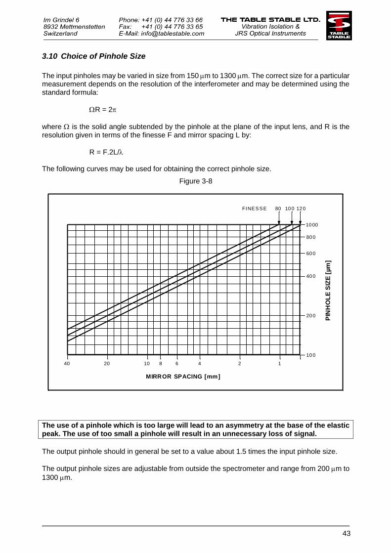
43

3.10 Choice of Pinhole Size

The input pinholes may be varied in size from 150 m to 1300 m. The correct size for a particular measurement depends on the resolution of the interferometer and may be determined using the standard formula:

R = 2

where is the solid angle subtended by the pinhole at the plane of the input lens, and R is the resolution given in terms of the finesse F and mirror spacing L by:

R = F.2L/ The following curves may be used for obtaining the correct pinhole size.

Figure 3-8

The use of a pinhole which is too large will lead to an asymmetry at the base of the elastic peak. The use of too small a pinhole will result in an unnecessary loss of signal.

The output pinhole should in general be set to a value about 1.5 times the input pinhole size.

The output pinhole sizes are adjustable from outside the spectrometer and range from 200 m to

1300 m.

10 0 12 080

10 82040

10 0

20 0

2 14

60 0

80 0

10 00

40 0

FINESSE

PIN

HO

LE

SIZ

E [

µm

]

MIRROR SPACING [mm]

6

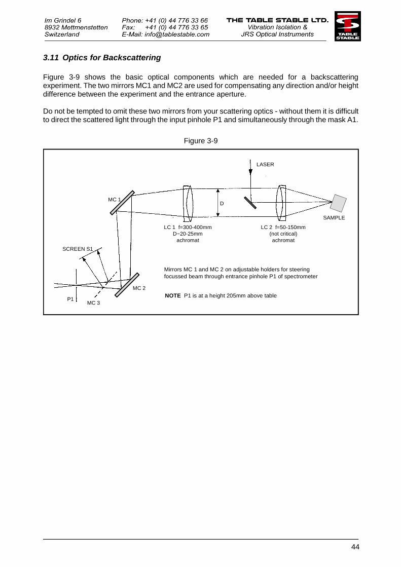
44

3.11 Optics for Backscattering

Figure 3-9 shows the basic optical components which are needed for a backscattering experiment. The two mirrors MC1 and MC2 are used for compensating any direction and/or height difference between the experiment and the entrance aperture. Do not be tempted to omit these two mirrors from your scattering optics - without them it is difficult to direct the scattered light through the input pinhole P1 and simultaneously through the mask A1.

Figure 3-9

LASER

SAMPLE

LC 1 f=300-400mm

D~20-25mm

achromat

LC 2 f=50-150mm

(not critical)

achromat

MC 1

MC 2

MC 3P1

SCREEN S1

D

Mirrors MC 1 and MC 2 on adjustable holders for steering

focussed beam through entrance pinhole P1 of spectrometer

NOTE P1 is at a height 205mm above table

45

3.12 Calibration of Mirror Spacings

The two interferometers of the tandem system will only scan synchronously if the relationship L2

= L1·cos ( is accurately maintained. In general there will be some error in Z so that L2= L1

cos (+ . For satisfactory scanning the error should be less than L1/500. Furthermore the wavelength scale of the spectrum depends on the mirror spacing so the accuracy of a measurement will depend on the absolute accuracy to which the mirror spacing can be read.

The calibration procedure is used to reduce as possible, and at the same time to set the spectrometer mirror spacing gauge to a correct value. The calibration requires the use of two lenses, a positive and a conical one, provided with the instrument. Using the interference rings created by the first calibration lens, the mirror spacings

may be calibrated to an accuracy of about 2-3 m, most of the error coming from reading the gauge. This is adequate for spacings greater than about 2 mm as used in typical Brillouin measurements. However for large frequency range, i.e. measurements where spacings of 1 mm

or less are used, the error in Z must be set much smaller. With the special conical lenses a

calibration error less than 0.25 m can be achieved. The calibration condition related to the conical lens is fulfilled when the spacing in FP1 is equal to 144 half-wavelengths. This means that

the calibration spacing will be, for example, about 38 m at 532 nm: this allows the use to calibrate the mirrors spacing indicator dial. The instrument calibration is set at factory and is often also checked after installation; it can be checked from time to time, especially when there is a need of performing measurements at a particularly small mirror spacing. A very efficient and quick method to check if the relative mirror spacing is correct, is to verify the transmission function of the instrument: when the mirror spacing is set at a small value, an error in the relative mirror spacing calibration will lead to uneven transmission function in the interferometer. In order to test the transmission function, after bringing the spectrometer to the normal work condition at the desired mirror spacing, a small incandescent bulb can be placed in the focus of the system to provide a good approximation of a black body radiation source. The spectrum observed by the instrument should look perfectly flat: any asymmetry in the signal indicates the need for a new calibration. In case a new calibration is needed, the related procedure is described in this manual at section 7.7.

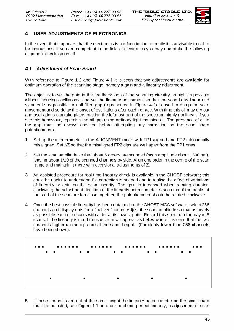
46

4 USER ADJUSTMENTS OF ELECTRONICS In the event that it appears that the electronics is not functioning correctly it is advisable to call in for instructions. If you are competent in the field of electronics you may undertake the following alignment checks yourself.

4.1 Adjustment of Scan Board

With reference to Figure 1-2 and Figure 4-1 it is seen that two adjustments are available for optimum operation of the scanning stage, namely a gain and a linearity adjustment. The object is to set the gain in the feedback loop of the scanning circuitry as high as possible without inducing oscillations, and set the linearity adjustment so that the scan is as linear and symmetric as possible. An oil filled gap (represented in Figure 4-2) is used to damp the scan movement and so delay the onset of oscillations after each retrace. With time this oil may dry out and oscillations can take place, making the leftmost part of the spectrum highly nonlinear. If you see this behaviour, replenish the oil gap using ordinary light machine oil. The presence of oil in the gap must be always checked before attempting any correction on the scan board potentiometers. 1. Set up the interferometer in the ALIGNMENT mode with FP1 aligned and FP2 intentionally

misaligned. Set Z so that the misaligned FP2 dips are well apart from the FP1 ones. 2. Set the scan amplitude so that about 5 orders are scanned (scan amplitude about 1300 nm),

leaving about 1/10 of the scanned channels by side. Align one order in the centre of the scan range and maintain it there with occasional adjustments of Z.

3. An assisted procedure for real-time linearity check is available in the GHOST software; this

could be useful to understand if a correction is needed and to realise the effect of variations of linearity or gain on the scan linearity. The gain is increased when rotating counter-clockwise; the adjustment direction of the linearity potentiometer is such that if the peaks at the start of the scan are too close together, the potentiometer should be rotated clockwise.

4. Once the best possible linearity has been obtained on the GHOST MCA software, select 256

channels and display dots for a final verification. Adjust the scan amplitude so that as nearly as possible each dip occurs with a dot at its lowest point. Record this spectrum for maybe 5 scans. If the linearity is good the spectrum will appear as below where it is seen that the two channels higher up the dips are at the same height. (For clarity fewer than 256 channels have been shown).

5. If these channels are not at the same height the linearity potentiometer on the scan board must be adjusted, see Figure 4-1, in order to obtain perfect linearity; readjustment of scan

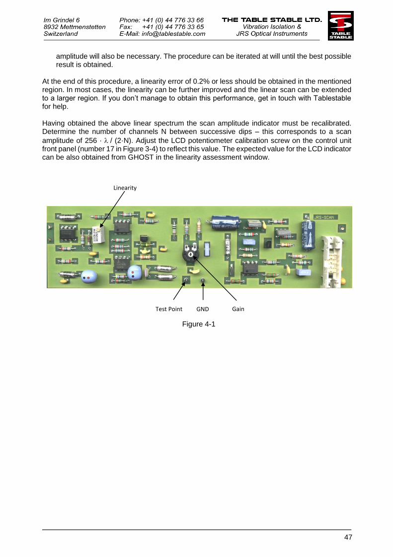
47

amplitude will also be necessary. The procedure can be iterated at will until the best possible result is obtained.

At the end of this procedure, a linearity error of 0.2% or less should be obtained in the mentioned region. In most cases, the linearity can be further improved and the linear scan can be extended to a larger region. If you don’t manage to obtain this performance, get in touch with Tablestable for help. Having obtained the above linear spectrum the scan amplitude indicator must be recalibrated. Determine the number of channels N between successive dips – this corresponds to a scan

amplitude of 256 · / (2·N). Adjust the LCD potentiometer calibration screw on the control unit front panel (number 17 in Figure 3-4) to reflect this value. The expected value for the LCD indicator can be also obtained from GHOST in the linearity assessment window.

Figure 4-1

Linearity

Gain GND Test Point

48

4.2 Further Adjustments

4.2.1 Adjustment of LCD display of scan amplitude

The LCD display indicates the total scan movement in nanometers. There is a potentiometer adjustment for calibration on the front panel just below the switch for changing the number of channels. An accurate calibration can be carried out as described above in section 4.1 following the adjustment of the scan linearity. An approximate calibration can be performed when in the alignment mode. Following the procedure described in section 0, detune FP2 so that only the dips of FP1 remain sharp. Centre one dip and adjust the scan amplitude until exactly two orders of FP1 are scanned – this is a scan

amplitude equal to (There is a small non-linearity for the first 4 ms at the beginning of the scan which makes the setting somewhat uncertain).

Adjust the potentiometer so that the LCD display shows the value of in nanometers.

4.2.2 Adjusting the Z scan movement

When adjusting the alignment of the interferometer in the alignment mode, an adjustment of Z is used to move the dips to coincidence. During this movement it is of course desirable that FP2 stays in alignment. In other words the movement of the FP2 mirror must be tilt-free. Unlike the Z-

scan movement which is determined by the movement of the parallelogram, the Z movement is achieved by movements of the three PZTs supporting the non-scanning mirror of FP2.

In order to make the movement tilt-free the fractions of the Z voltage applied to each of the PZTs must be adjusted to allow for the differing characteristics of the PZTs. This adjustment has been performed at the factory and it is unlikely that you will need to change it. Should it however become necessary, the procedure is relatively straightforward. Remove the 7 knobs from the front panel controls of the control unit and remove the front panel. Pull out board no. 2 (the second from the left) and reconnect using an extender board. You will observe two potentiometers on this board. In the alignment mode observe the dips due to FP2. Set the scan amplitude to about 100nm so that only one dip is seen.

Adjust the Z control so that the Z display is mid-range. Optimize the alignment of FP2 using the motor controls with the PZT controls set to mid-range. Adjust Z if necessary to bring the dip

to mid scan. Now turn the Z control so that Z is scanned by one order. If the scan is tilt-free the alignment of FP2 should remain optimum – if not, adjust the two potentiometers on board 2 until full alignment is achieved again.

Scan Z over the whole range and check for good alignment. Repeat the above procedure if necessary.

49

4.3 Adjustment of Capacitance Range and Centring of Scan Amplitude Indicator

The scan amplitude LED indicator on the control unit front panel (14) could be occasionally found off center. This happens usually when the room temperature has changed noticeably and thermal expansion of the system components has modified the scanning stage capacitor spacing, so that the indicator mid range does not corresponds anymore with the reference mid range capacity. This phenomenon is normal and not harmful. If the indicator is far from midrange the scan amplitude will be compromised. The instrument needs to be adjusted by bringing the capacitance into the correct range. This operation is very quick and easy to do. In order to adjust the spacing of the capacitor and compensate these thermal variations:

Set a zero scan amplitude and switch off the detector, then open the lid of the instrument. Using a zero scan amplitude, you will see a single LED lit in the scan amplitude indicator.

Looking at the scan stage and with reference to Figure 4-2, locate the transducer adjust screw A. This screw has a series of small transverse holes that allow one to turn it from the side. On the TFP-2, these holes could be not accessible at large mirror spacing: if this happens, reduce the mirror spacing as necessary by using the Z motor.

Insert the special needle tip tool provided by the spectrometer in one of the holes on screw A and turn the screw gently and by a very small angle until the scan amplitude LED moves to the center (yellow LED). The sense of motion is such that, if the reported position is higher than the central LED, you must push the tool, and vice versa.

If difficulty has been experienced in setting the scan-amplitude indicator to mid-range or if highly non-linear scanning is suspected, it may be necessary to reset the capacitance and the scanning transducer. The related procedure is described at end of section 3.1.1.

50

Figure 4-2

TRANSDUCER ADJUSTSCREW

TRANSDUCER

CAPACITANCEMOUNTING BLOCK

TO CAPACITANCECAPACITANCE CLAMP SCREW

SPRING

30 m SPACER

30 m GAP (CONTAINSOIL FOR DAMPING)

HV TOTRANSDUCER

SCAN STOP

CAPACITOR

TRANSDUCER ADJUST SCREW A

SCREW B (SPRING LOADED)

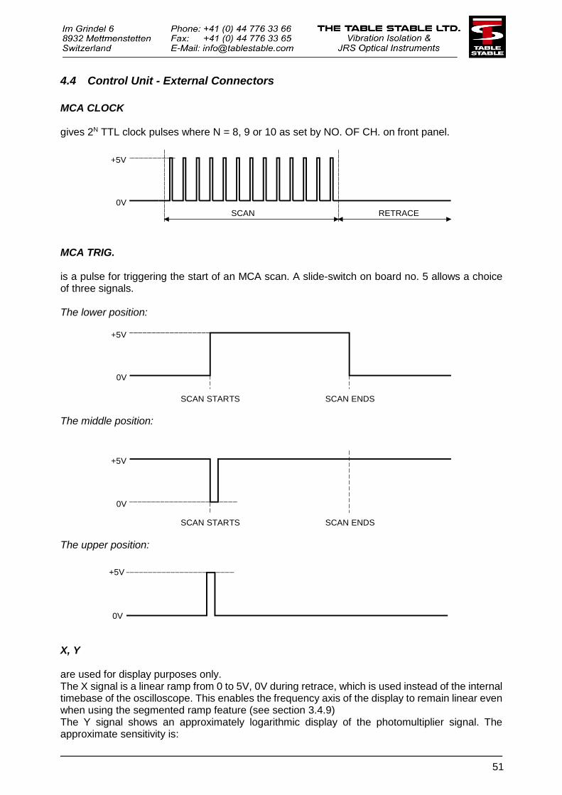
51

4.4 Control Unit - External Connectors

MCA CLOCK gives 2N TTL clock pulses where N = 8, 9 or 10 as set by NO. OF CH. on front panel.

SCAN RETRACE

0V

+5V

MCA TRIG. is a pulse for triggering the start of an MCA scan. A slide-switch on board no. 5 allows a choice of three signals. The lower position:

0V

+5V

SCAN STARTS SCAN ENDS The middle position:

0V

+5V

SCAN STARTS SCAN ENDS The upper position:

X, Y are used for display purposes only. The X signal is a linear ramp from 0 to 5V, 0V during retrace, which is used instead of the internal timebase of the oscilloscope. This enables the frequency axis of the display to remain linear even when using the segmented ramp feature (see section 3.4.9) The Y signal shows an approximately logarithmic display of the photomultiplier signal. The approximate sensitivity is:

0V

+5V

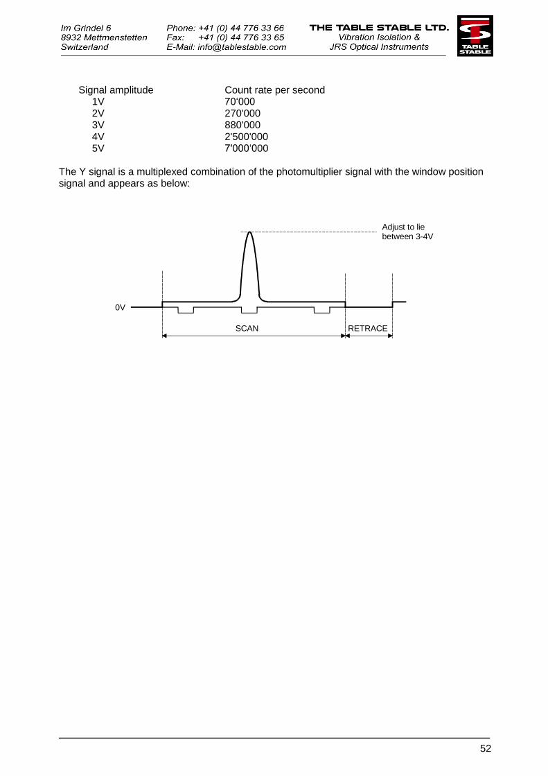
52

Signal amplitude Count rate per second

1V 70‘000 2V 270'000 3V 880'000 4V 2'500'000 5V 7'000‘000 The Y signal is a multiplexed combination of the photomultiplier signal with the window position signal and appears as below:

SCAN RETRACE

Adjust to liebetween 3-4V

0V

53

4.5 Interferometer Control Unit Remote Control Inputs

On the rear panel of the control unit is a D-Sub 15 F socket allowing remote control of some of the control unit functions. The pin connections are given below: 1 -5V 2 +5V

3 Z (+5V to –5V) 4 Y2 (+5V to –5V) 5 X2 (+5V to –5V) 6 Y1 (+5V to –5V) 7 X1 (+5V to –5V) 8 Align (TTL out) 9 GND 10 TTL input (Optics, 1 Align, 0 Tandem) 11 TTL input (PM shutter, 1 open) 12 TTL input (Input shutter, 1 opens SH1 and closes SH2) NB. Shutter switch to "window“! 13 Vz output (+5V to –5V, impedance 68K, proportional to voltage on scan PZT) 14 Vscan input Z (+5V to –5V) 15 Busy (TTL out) – optical system changing mode. D-Sub 25 connection from Control Unit to Interferometer 1 X1 brown -50 to 0 V (or -60 to 0 V)* 2 Y1 (TOP) orange -50 to 0 V (or -60 to 0 V)*

3 X2+Z green -100 to 0 V (or -120 to 0 V)* 4 +250V mauve 5 –250V white 6 GND brown 7 Vz (out) orange 8 Vscan green 9 Align (out) mauve 10 Busy white 11 PM shutter gnd brown 12 PM shutter TTL in orange 13 GND green 14 Y1 (BOTTOM) red 0 to 50 V (or 0 to 60 V)*

15 Y2+Z (TOP) yellow -100 to 0 V (or -120 to 0 V)*

16 Y2–Z (BOTTOM) blue 0 to 100 V (or 0 to 120)* 17 NC grey 18 NC black 19 GND red 20 +5V yellow 21 –5V blue 22 NC grey 23 TTL (in) black 0 for Tandem, 1 for Alignment 24 +5V red 25 +5V yellow

* The voltage range reported in brackets refers to instruments sold before December 2014.

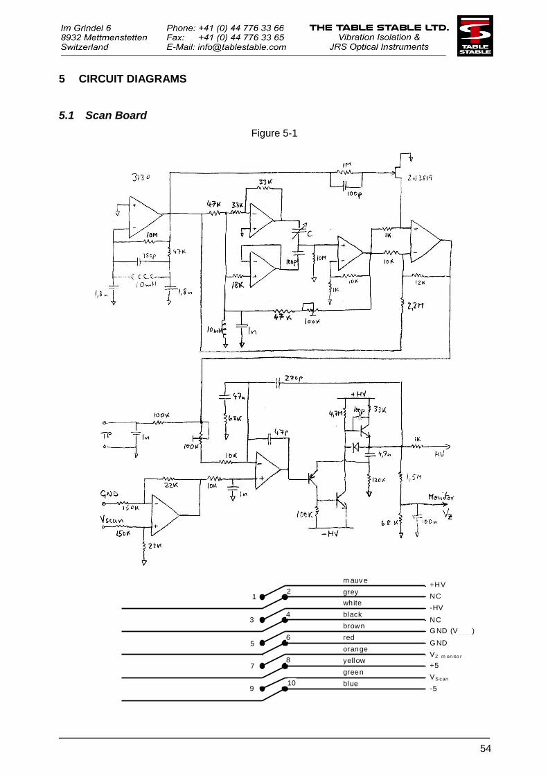
54

5 CIRCUIT DIAGRAMS

5.1 Scan Board

Figure 5-1

yellow

orange

red

brown

-5

GND

S canGND (V )

VZ

V

+5

m on ito r

S can

white

grey

m auv e+HV

NC

-HV

2

3black

NC

9

7

5

1

blue

green

4

6

8

10

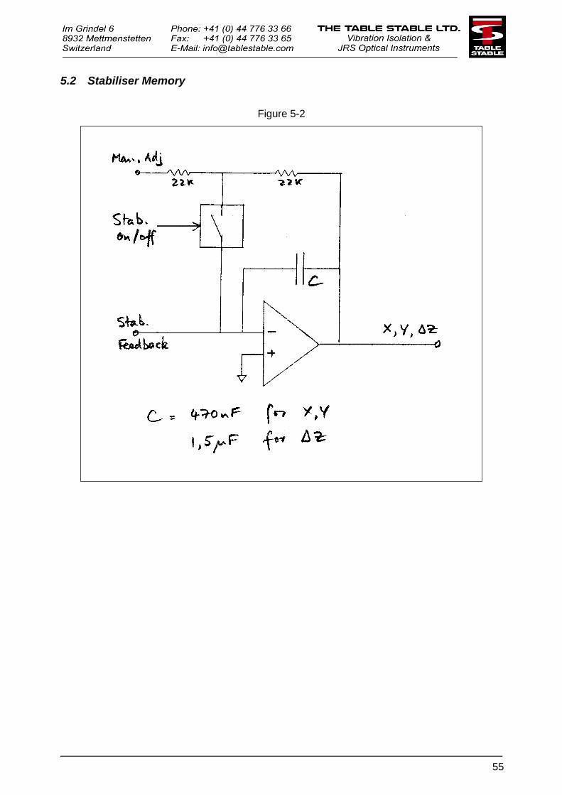
55

5.2 Stabiliser Memory

Figure 5-2

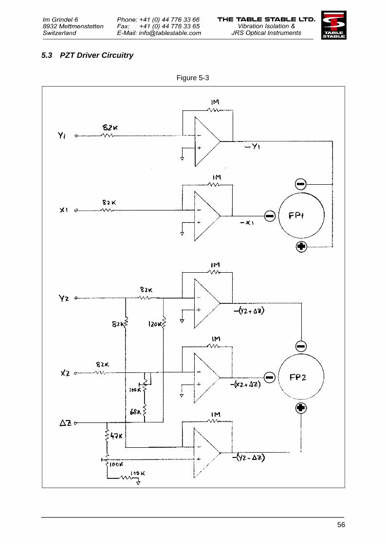
56

5.3 PZT Driver Circuitry

Figure 5-3

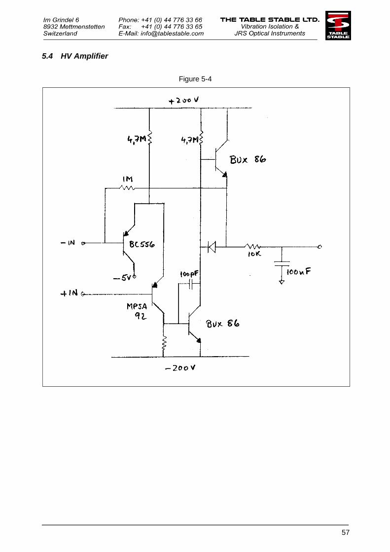
57

5.4 HV Amplifier

Figure 5-4

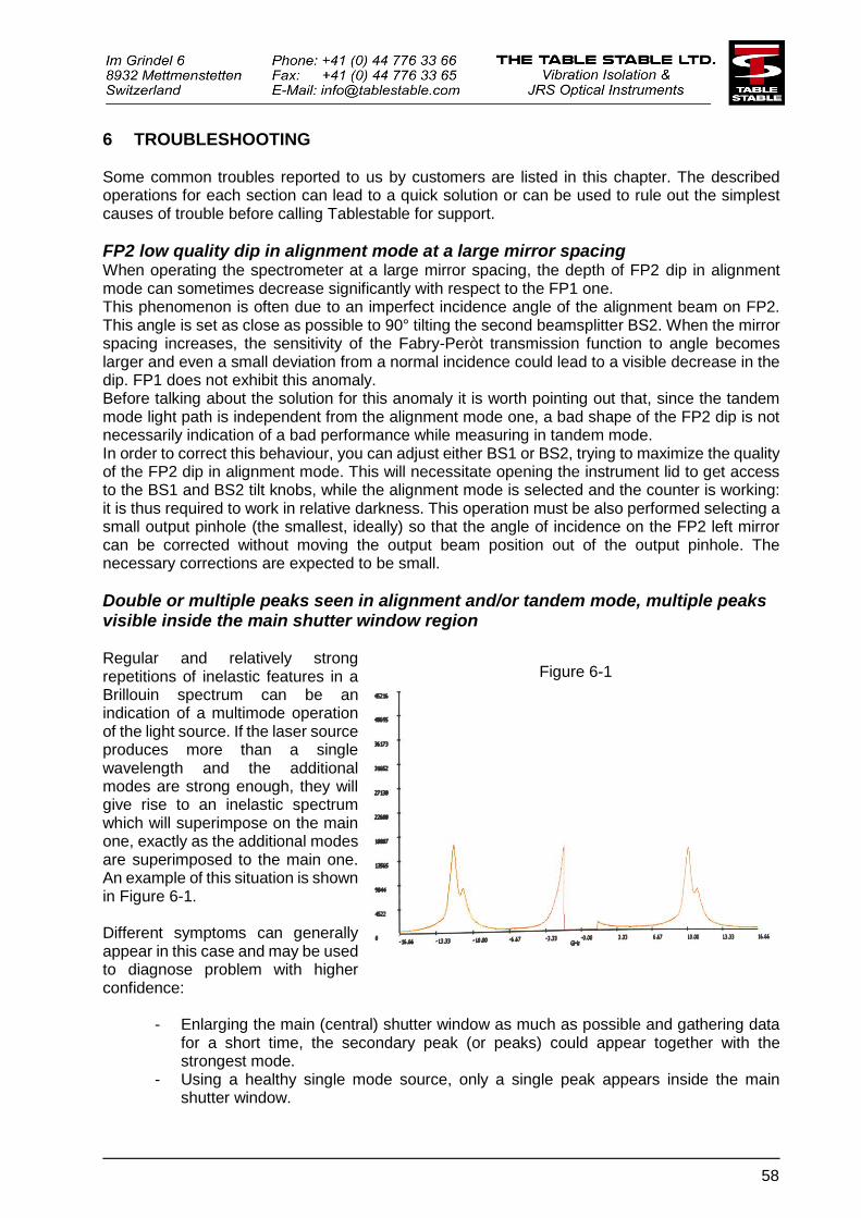
58

6 TROUBLESHOOTING Some common troubles reported to us by customers are listed in this chapter. The described operations for each section can lead to a quick solution or can be used to rule out the simplest causes of trouble before calling Tablestable for support.

FP2 low quality dip in alignment mode at a large mirror spacing When operating the spectrometer at a large mirror spacing, the depth of FP2 dip in alignment mode can sometimes decrease significantly with respect to the FP1 one. This phenomenon is often due to an imperfect incidence angle of the alignment beam on FP2. This angle is set as close as possible to 90° tilting the second beamsplitter BS2. When the mirror spacing increases, the sensitivity of the Fabry-Peròt transmission function to angle becomes larger and even a small deviation from a normal incidence could lead to a visible decrease in the dip. FP1 does not exhibit this anomaly. Before talking about the solution for this anomaly it is worth pointing out that, since the tandem mode light path is independent from the alignment mode one, a bad shape of the FP2 dip is not necessarily indication of a bad performance while measuring in tandem mode. In order to correct this behaviour, you can adjust either BS1 or BS2, trying to maximize the quality of the FP2 dip in alignment mode. This will necessitate opening the instrument lid to get access to the BS1 and BS2 tilt knobs, while the alignment mode is selected and the counter is working: it is thus required to work in relative darkness. This operation must be also performed selecting a small output pinhole (the smallest, ideally) so that the angle of incidence on the FP2 left mirror can be corrected without moving the output beam position out of the output pinhole. The necessary corrections are expected to be small.

Double or multiple peaks seen in alignment and/or tandem mode, multiple peaks visible inside the main shutter window region Regular and relatively strong repetitions of inelastic features in a Brillouin spectrum can be an indication of a multimode operation of the light source. If the laser source produces more than a single wavelength and the additional modes are strong enough, they will give rise to an inelastic spectrum which will superimpose on the main one, exactly as the additional modes are superimposed to the main one. An example of this situation is shown in Figure 6-1. Different symptoms can generally appear in this case and may be used to diagnose problem with higher confidence:

- Enlarging the main (central) shutter window as much as possible and gathering data for a short time, the secondary peak (or peaks) could appear together with the strongest mode.

- Using a healthy single mode source, only a single peak appears inside the main shutter window.

Figure 6-1

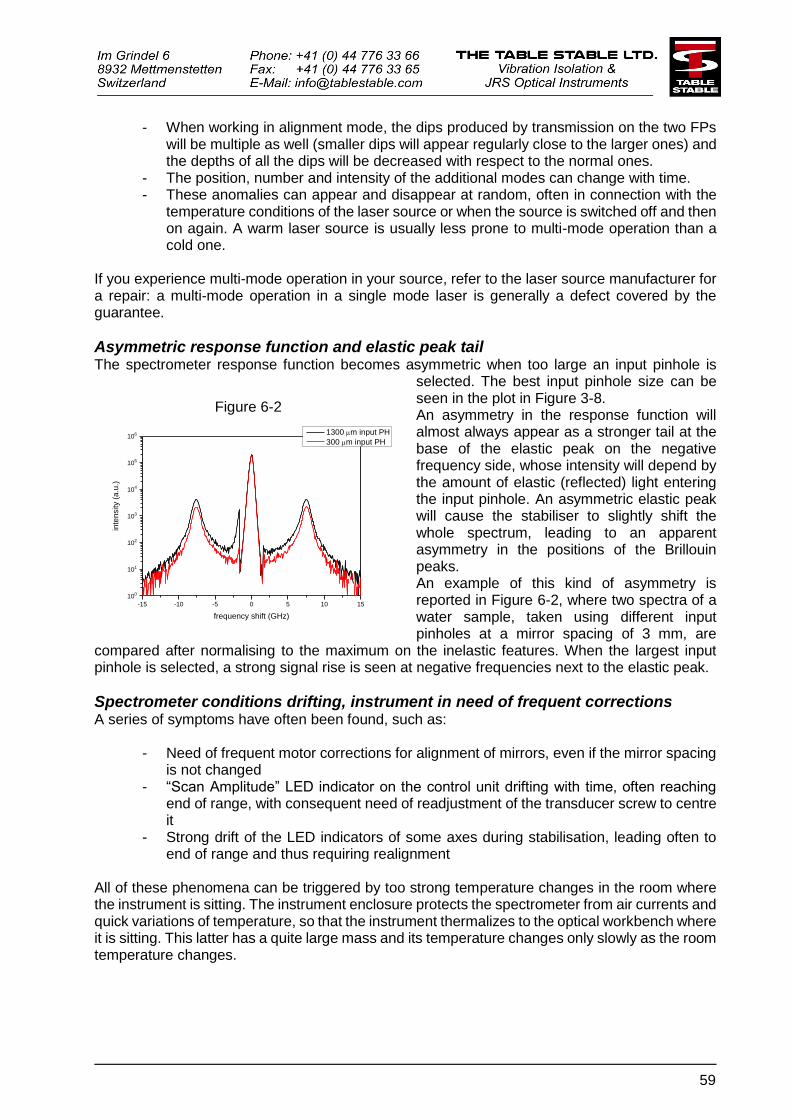
59

- When working in alignment mode, the dips produced by transmission on the two FPs will be multiple as well (smaller dips will appear regularly close to the larger ones) and the depths of all the dips will be decreased with respect to the normal ones.

- The position, number and intensity of the additional modes can change with time. - These anomalies can appear and disappear at random, often in connection with the

temperature conditions of the laser source or when the source is switched off and then on again. A warm laser source is usually less prone to multi-mode operation than a cold one.

If you experience multi-mode operation in your source, refer to the laser source manufacturer for a repair: a multi-mode operation in a single mode laser is generally a defect covered by the guarantee.

Asymmetric response function and elastic peak tail The spectrometer response function becomes asymmetric when too large an input pinhole is

selected. The best input pinhole size can be seen in the plot in Figure 3-8. An asymmetry in the response function will almost always appear as a stronger tail at the base of the elastic peak on the negative frequency side, whose intensity will depend by the amount of elastic (reflected) light entering the input pinhole. An asymmetric elastic peak will cause the stabiliser to slightly shift the whole spectrum, leading to an apparent asymmetry in the positions of the Brillouin peaks. An example of this kind of asymmetry is reported in Figure 6-2, where two spectra of a water sample, taken using different input pinholes at a mirror spacing of 3 mm, are

compared after normalising to the maximum on the inelastic features. When the largest input pinhole is selected, a strong signal rise is seen at negative frequencies next to the elastic peak.

Spectrometer conditions drifting, instrument in need of frequent corrections A series of symptoms have often been found, such as:

- Need of frequent motor corrections for alignment of mirrors, even if the mirror spacing is not changed

- “Scan Amplitude” LED indicator on the control unit drifting with time, often reaching end of range, with consequent need of readjustment of the transducer screw to centre it

- Strong drift of the LED indicators of some axes during stabilisation, leading often to end of range and thus requiring realignment

All of these phenomena can be triggered by too strong temperature changes in the room where the instrument is sitting. The instrument enclosure protects the spectrometer from air currents and quick variations of temperature, so that the instrument thermalizes to the optical workbench where it is sitting. This latter has a quite large mass and its temperature changes only slowly as the room temperature changes.

Figure 6-2

-15 -10 -5 0 5 10 15

100

101

102

103

104

105

106

inte

nsity (

a.u

.)

frequency shift (GHz)

1300 m input PH

300 m input PH

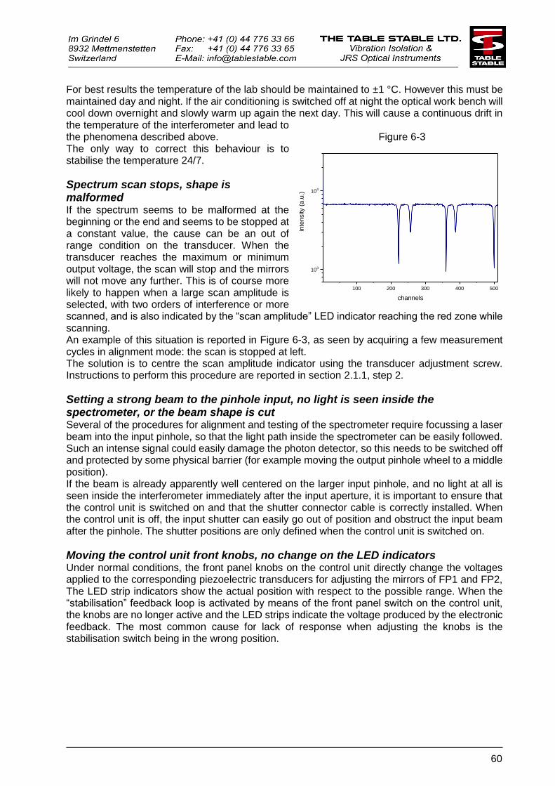
60

For best results the temperature of the lab should be maintained to ±1 °C. However this must be maintained day and night. If the air conditioning is switched off at night the optical work bench will cool down overnight and slowly warm up again the next day. This will cause a continuous drift in the temperature of the interferometer and lead to the phenomena described above. The only way to correct this behaviour is to stabilise the temperature 24/7.

Spectrum scan stops, shape is malformed If the spectrum seems to be malformed at the beginning or the end and seems to be stopped at a constant value, the cause can be an out of range condition on the transducer. When the transducer reaches the maximum or minimum output voltage, the scan will stop and the mirrors will not move any further. This is of course more likely to happen when a large scan amplitude is selected, with two orders of interference or more scanned, and is also indicated by the “scan amplitude” LED indicator reaching the red zone while scanning. An example of this situation is reported in Figure 6-3, as seen by acquiring a few measurement cycles in alignment mode: the scan is stopped at left. The solution is to centre the scan amplitude indicator using the transducer adjustment screw. Instructions to perform this procedure are reported in section 2.1.1, step 2.

Setting a strong beam to the pinhole input, no light is seen inside the spectrometer, or the beam shape is cut Several of the procedures for alignment and testing of the spectrometer require focussing a laser beam into the input pinhole, so that the light path inside the spectrometer can be easily followed. Such an intense signal could easily damage the photon detector, so this needs to be switched off and protected by some physical barrier (for example moving the output pinhole wheel to a middle position). If the beam is already apparently well centered on the larger input pinhole, and no light at all is seen inside the interferometer immediately after the input aperture, it is important to ensure that the control unit is switched on and that the shutter connector cable is correctly installed. When the control unit is off, the input shutter can easily go out of position and obstruct the input beam after the pinhole. The shutter positions are only defined when the control unit is switched on.

Moving the control unit front knobs, no change on the LED indicators Under normal conditions, the front panel knobs on the control unit directly change the voltages applied to the corresponding piezoelectric transducers for adjusting the mirrors of FP1 and FP2, The LED strip indicators show the actual position with respect to the possible range. When the “stabilisation” feedback loop is activated by means of the front panel switch on the control unit, the knobs are no longer active and the LED strips indicate the voltage produced by the electronic feedback. The most common cause for lack of response when adjusting the knobs is the stabilisation switch being in the wrong position.

Figure 6-3

100 200 300 400 500

103

104

inte

nsity (

a.u

.)channels

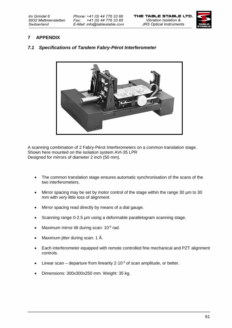
61

7 APPENDIX

7.1 Specifications of Tandem Fabry-Pérot Interferometer

A scanning combination of 2 Fabry-Pérot Interferometers on a common translation stage. Shown here mounted on the isolation system AVI-35 LPR Designed for mirrors of diameter 2 inch (50 mm).

The common translation stage ensures automatic synchronisation of the scans of the two interferometers.

Mirror spacing may be set by motor control of the stage within the range 30 µm to 30 mm with very little loss of alignment.

Mirror spacing read directly by means of a dial gauge.

Scanning range 0-2.5 µm using a deformable parallelogram scanning stage.

Maximum mirror tilt during scan: 10-8 rad.

Maximum jitter during scan: 1 Å.

Each interferometer equipped with remote controlled fine mechanical and PZT alignment controls.

Linear scan – departure from linearity 2·10-3 of scan amplitude, or better.

Dimensions: 300x300x250 mm. Weight: 35 kg.

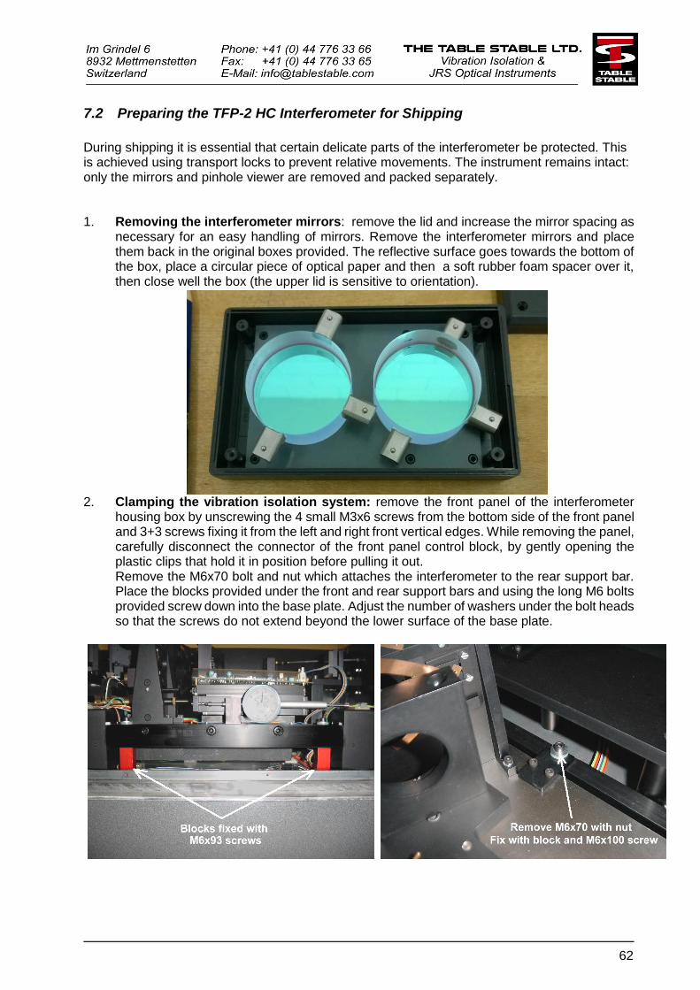
62

7.2 Preparing the TFP-2 HC Interferometer for Shipping

During shipping it is essential that certain delicate parts of the interferometer be protected. This is achieved using transport locks to prevent relative movements. The instrument remains intact: only the mirrors and pinhole viewer are removed and packed separately.

1. Removing the interferometer mirrors: remove the lid and increase the mirror spacing as necessary for an easy handling of mirrors. Remove the interferometer mirrors and place them back in the original boxes provided. The reflective surface goes towards the bottom of the box, place a circular piece of optical paper and then a soft rubber foam spacer over it, then close well the box (the upper lid is sensitive to orientation).

2. Clamping the vibration isolation system: remove the front panel of the interferometer housing box by unscrewing the 4 small M3x6 screws from the bottom side of the front panel and 3+3 screws fixing it from the left and right front vertical edges. While removing the panel, carefully disconnect the connector of the front panel control block, by gently opening the plastic clips that hold it in position before pulling it out. Remove the M6x70 bolt and nut which attaches the interferometer to the rear support bar. Place the blocks provided under the front and rear support bars and using the long M6 bolts provided screw down into the base plate. Adjust the number of washers under the bolt heads so that the screws do not extend beyond the lower surface of the base plate.

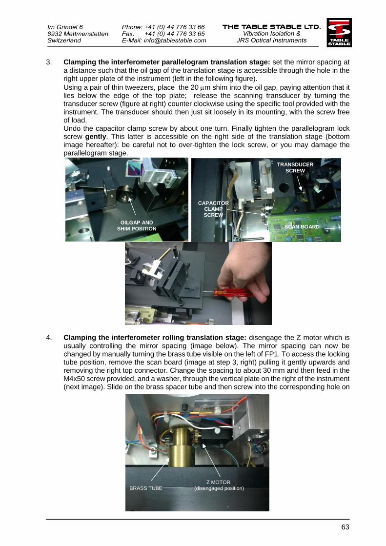
63

3. Clamping the interferometer parallelogram translation stage: set the mirror spacing at a distance such that the oil gap of the translation stage is accessible through the hole in the right upper plate of the instrument (left in the following figure).

Using a pair of thin tweezers, place the 20 m shim into the oil gap, paying attention that it lies below the edge of the top plate; release the scanning transducer by turning the transducer screw (figure at right) counter clockwise using the specific tool provided with the instrument. The transducer should then just sit loosely in its mounting, with the screw free of load. Undo the capacitor clamp screw by about one turn. Finally tighten the parallelogram lock screw gently. This latter is accessible on the right side of the translation stage (bottom image hereafter): be careful not to over-tighten the lock screw, or you may damage the parallelogram stage.

4. Clamping the interferometer rolling translation stage: disengage the Z motor which is

usually controlling the mirror spacing (image below). The mirror spacing can now be changed by manually turning the brass tube visible on the left of FP1. To access the locking tube position, remove the scan board (image at step 3, right) pulling it gently upwards and removing the right top connector. Change the spacing to about 30 mm and then feed in the M4x50 screw provided, and a washer, through the vertical plate on the right of the instrument (next image). Slide on the brass spacer tube and then screw into the corresponding hole on

CAPACITOR CLAMP SCREW

TRANSDUCER

SCREW

SCAN BOARD

BRASS TUBE Z MOTOR

(disengaged position)

OILGAP AND

SHIM POSITION

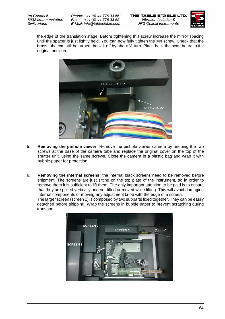
64

the edge of the translation stage. Before tightening this screw increase the mirror spacing until the spacer is just lightly held. You can now fully tighten the M4 screw. Check that the brass tube can still be turned: back it off by about ½ turn. Place back the scan board in the original position.

5. Removing the pinhole viewer: Remove the pinhole viewer camera by undoing the two

screws at the base of the camera tube and replace the original cover on the top of the shutter unit, using the same screws. Close the camera in a plastic bag and wrap it with bubble paper for protection.

6. Removing the internal screens: the internal black screens need to be removed before

shipment. The screens are just sitting on the top plate of the instrument, so in order to remove them it is sufficient to lift them. The only important attention to be paid is to ensure that they are pulled vertically and not tilted or moved while lifting. This will avoid damaging internal components or moving any adjustment knob with the edge of a screen. The larger screen (screen 1) is composed by two subparts fixed together. They can be easily detached before shipping. Wrap the screens in bubble paper to prevent scratching during transport.

SCREW M4x50

BRASS SPACER

SCREEN 2

SCREEN 3

SCREEN 1

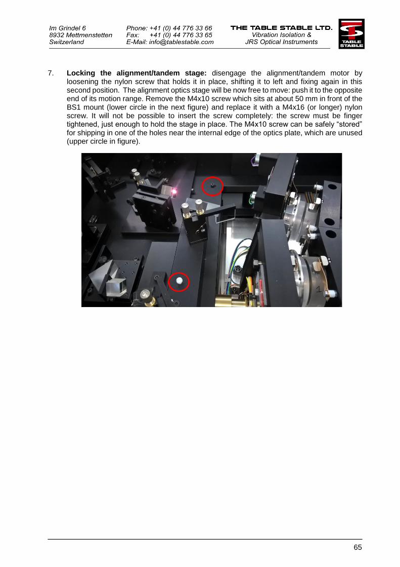
65

7. Locking the alignment/tandem stage: disengage the alignment/tandem motor by

loosening the nylon screw that holds it in place, shifting it to left and fixing again in this second position. The alignment optics stage will be now free to move: push it to the opposite end of its motion range. Remove the M4x10 screw which sits at about 50 mm in front of the BS1 mount (lower circle in the next figure) and replace it with a M4x16 (or longer) nylon screw. It will not be possible to insert the screw completely: the screw must be finger tightened, just enough to hold the stage in place. The M4x10 screw can be safely “stored” for shipping in one of the holes near the internal edge of the optics plate, which are unused (upper circle in figure).

SCREEN 1

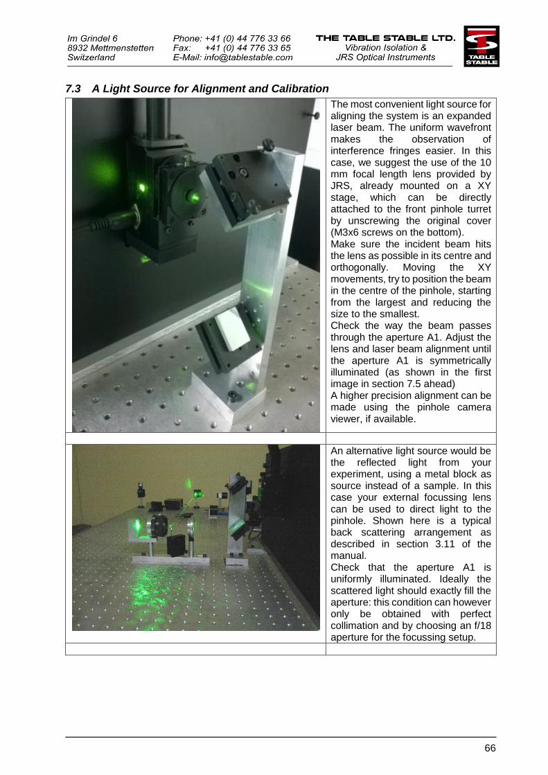
66

7.3 A Light Source for Alignment and Calibration

The most convenient light source for aligning the system is an expanded laser beam. The uniform wavefront makes the observation of interference fringes easier. In this case, we suggest the use of the 10 mm focal length lens provided by JRS, already mounted on a XY stage, which can be directly attached to the front pinhole turret by unscrewing the original cover (M3x6 screws on the bottom). Make sure the incident beam hits the lens as possible in its centre and orthogonally. Moving the XY movements, try to position the beam in the centre of the pinhole, starting from the largest and reducing the size to the smallest. Check the way the beam passes through the aperture A1. Adjust the lens and laser beam alignment until the aperture A1 is symmetrically illuminated (as shown in the first image in section 7.5 ahead) A higher precision alignment can be made using the pinhole camera viewer, if available.

An alternative light source would be the reflected light from your experiment, using a metal block as source instead of a sample. In this case your external focussing lens can be used to direct light to the pinhole. Shown here is a typical back scattering arrangement as described in section 3.11 of the manual. Check that the aperture A1 is uniformly illuminated. Ideally the scattered light should exactly fill the aperture: this condition can however only be obtained with perfect collimation and by choosing an f/18 aperture for the focussing setup.

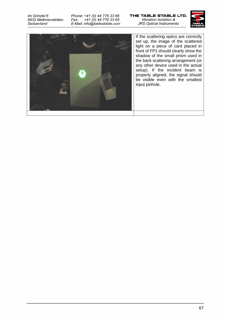
67

If the scattering optics are correctly set up, the image of the scattered light on a piece of card placed in front of FP1 should clearly show the shadow of the small prism used in the back scattering arrangement (or any other device used in the actual setup). If the incident beam is properly aligned, the signal should be visible even with the smallest input pinhole.

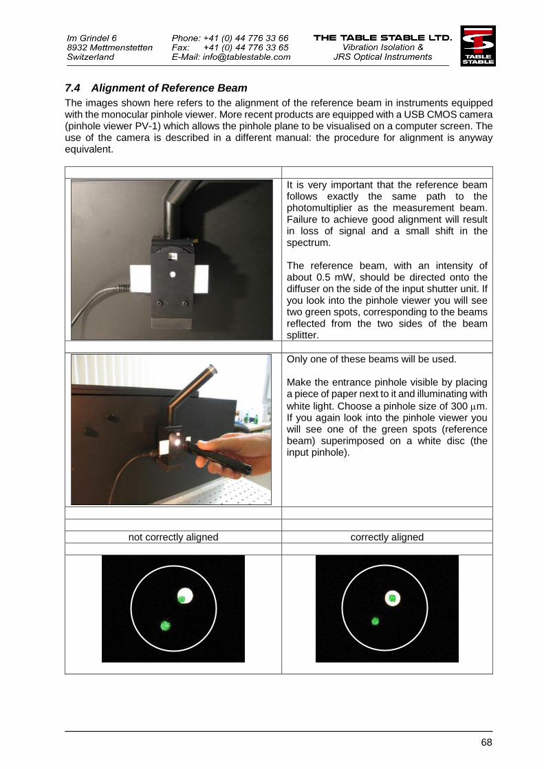
68

7.4 Alignment of Reference Beam

The images shown here refers to the alignment of the reference beam in instruments equipped with the monocular pinhole viewer. More recent products are equipped with a USB CMOS camera (pinhole viewer PV-1) which allows the pinhole plane to be visualised on a computer screen. The use of the camera is described in a different manual: the procedure for alignment is anyway equivalent.

It is very important that the reference beam follows exactly the same path to the photomultiplier as the measurement beam. Failure to achieve good alignment will result in loss of signal and a small shift in the spectrum. The reference beam, with an intensity of about 0.5 mW, should be directed onto the diffuser on the side of the input shutter unit. If you look into the pinhole viewer you will see two green spots, corresponding to the beams reflected from the two sides of the beam splitter.

Only one of these beams will be used. Make the entrance pinhole visible by placing a piece of paper next to it and illuminating with

white light. Choose a pinhole size of 300 m. If you again look into the pinhole viewer you will see one of the green spots (reference beam) superimposed on a white disc (the input pinhole).

not correctly aligned correctly aligned

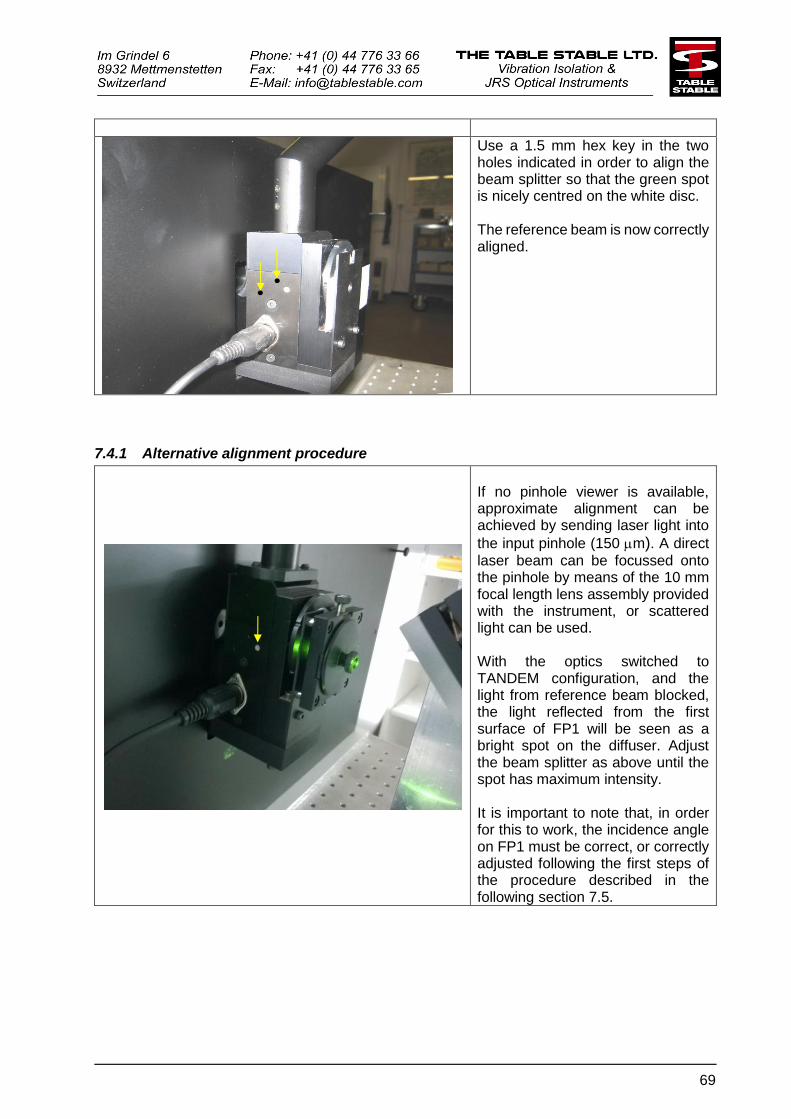
69

Use a 1.5 mm hex key in the two holes indicated in order to align the beam splitter so that the green spot is nicely centred on the white disc. The reference beam is now correctly aligned.

7.4.1 Alternative alignment procedure

If no pinhole viewer is available, approximate alignment can be achieved by sending laser light into

the input pinhole (150 m). A direct

laser beam can be focussed onto the pinhole by means of the 10 mm focal length lens assembly provided with the instrument, or scattered light can be used. With the optics switched to TANDEM configuration, and the light from reference beam blocked, the light reflected from the first surface of FP1 will be seen as a bright spot on the diffuser. Adjust the beam splitter as above until the spot has maximum intensity. It is important to note that, in order for this to work, the incidence angle on FP1 must be correct, or correctly adjusted following the first steps of the procedure described in the following section 7.5.

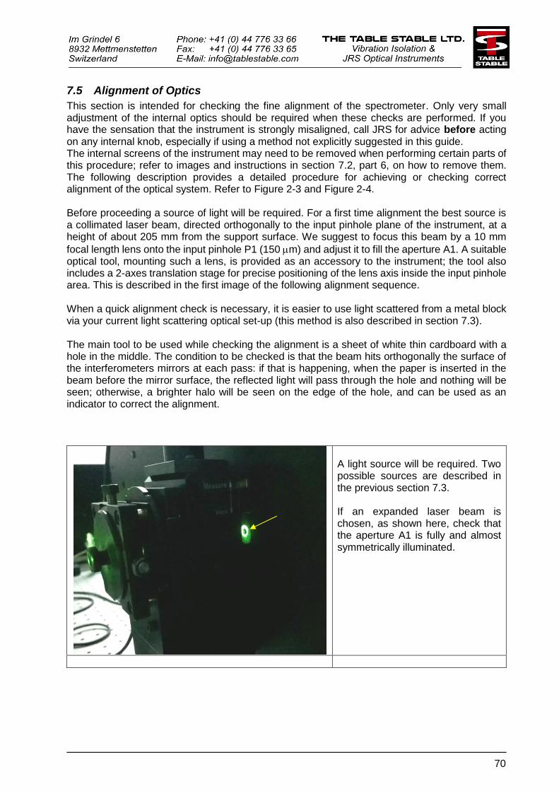
70

7.5 Alignment of Optics

This section is intended for checking the fine alignment of the spectrometer. Only very small adjustment of the internal optics should be required when these checks are performed. If you have the sensation that the instrument is strongly misaligned, call JRS for advice before acting on any internal knob, especially if using a method not explicitly suggested in this guide. The internal screens of the instrument may need to be removed when performing certain parts of this procedure; refer to images and instructions in section 7.2, part 6, on how to remove them. The following description provides a detailed procedure for achieving or checking correct alignment of the optical system. Refer to Figure 2-3 and Figure 2-4. Before proceeding a source of light will be required. For a first time alignment the best source is a collimated laser beam, directed orthogonally to the input pinhole plane of the instrument, at a height of about 205 mm from the support surface. We suggest to focus this beam by a 10 mm

focal length lens onto the input pinhole P1 (150 m) and adjust it to fill the aperture A1. A suitable optical tool, mounting such a lens, is provided as an accessory to the instrument; the tool also includes a 2-axes translation stage for precise positioning of the lens axis inside the input pinhole area. This is described in the first image of the following alignment sequence. When a quick alignment check is necessary, it is easier to use light scattered from a metal block via your current light scattering optical set-up (this method is also described in section 7.3). The main tool to be used while checking the alignment is a sheet of white thin cardboard with a hole in the middle. The condition to be checked is that the beam hits orthogonally the surface of the interferometers mirrors at each pass: if that is happening, when the paper is inserted in the beam before the mirror surface, the reflected light will pass through the hole and nothing will be seen; otherwise, a brighter halo will be seen on the edge of the hole, and can be used as an indicator to correct the alignment.

A light source will be required. Two possible sources are described in the previous section 7.3. If an expanded laser beam is chosen, as shown here, check that the aperture A1 is fully and almost symmetrically illuminated.

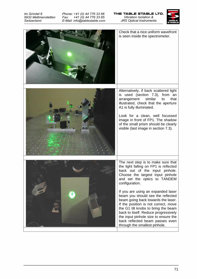
71

Check that a nice uniform wavefront is seen inside the spectrometer.

Alternatively, if back scattered light is used (section 7.3), from an arrangement similar to that illustrated, check that the aperture A1 is fully illuminated. Look for a clean, well focussed image in front of FP1. The shadow of the small prism should be clearly visible (last image in section 7.3).

The next step is to make sure that the light falling on FP1 is reflected back out of the input pinhole. Choose the largest input pinhole and set the optics to TANDEM configuration. If you are using an expanded laser beam you should see the reflected beam going back towards the laser. If the position is not correct, move the G1 tilt knobs to bring the beam back to itself. Reduce progressively the input pinhole size to ensure the back reflected beam passes even through the smallest pinhole.

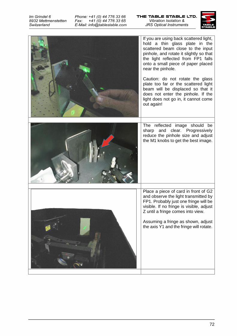
72

If you are using back scattered light, hold a thin glass plate in the scattered beam close to the input pinhole, and rotate it slightly so that the light reflected from FP1 falls onto a small piece of paper placed near the pinhole. Caution: do not rotate the glass plate too far or the scattered light beam will be displaced so that it does not enter the pinhole. If the light does not go in, it cannot come out again!

The reflected image should be sharp and clear. Progressively reduce the pinhole size and adjust the M1 knobs to get the best image.

Place a piece of card in front of G2 and observe the light transmitted by FP1. Probably just one fringe will be visible. If no fringe is visible, adjust Z until a fringe comes into view. Assuming a fringe as shown, adjust the axis Y1 and the fringe will rotate.

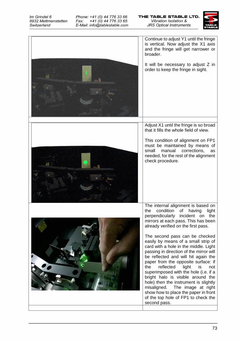
73

Continue to adjust Y1 until the fringe is vertical. Now adjust the X1 axis and the fringe will get narrower or broader. It will be necessary to adjust Z in order to keep the fringe in sight.

Adjust X1 until the fringe is so broad that it fills the whole field of view. This condition of alignment on FP1 must be maintained by means of small manual corrections, as needed, for the rest of the alignment check procedure.

The internal alignment is based on the condition of having light perpendicularly incident on the mirrors at each pass. This has been already verified on the first pass. The second pass can be checked easily by means of a small strip of card with a hole in the middle. Light passing in direction of the mirror will be reflected and will hit again the paper from the opposite surface: if the reflected light is not superimposed with the hole (i.e. if a bright halo is visible around the hole) then the instrument is slightly misaligned. The image at right show how to place the paper in front of the top hole of FP1 to check the second pass.

74

If the second pass appears misaligned, you can adjust the

incidence of light by using the knob indicated in the figure here at left.

If a /4 alignment tool was provided together the instrument, a more

sensitive test of alignment can be performed following the indications

reported in section 7.6.

Similarly, the third pass incidence angle can be checked by observing the card when it is positioned at left of FP1, going to the bottom right hole.

To align the third pass, the knob to be used is shown here at right. This concludes the checks for all the passes through FP1.

Follow the beam though the third pass, towards G4 and FP2. Check the orthogonal incidence condition on FP2 with the paper; small misalignments could be corrected by means of G4 tilt knobs.

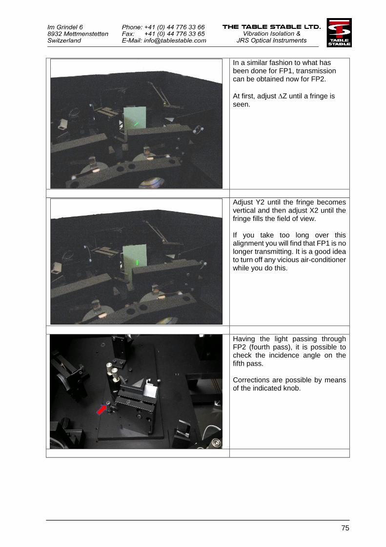
75

In a similar fashion to what has been done for FP1, transmission can be obtained now for FP2.

At first, adjust Z until a fringe is seen.

Adjust Y2 until the fringe becomes vertical and then adjust X2 until the fringe fills the field of view. If you take too long over this alignment you will find that FP1 is no longer transmitting. It is a good idea to turn off any vicious air-conditioner while you do this.

Having the light passing through FP2 (fourth pass), it is possible to check the incidence angle on the fifth pass. Corrections are possible by means of the indicated knob.

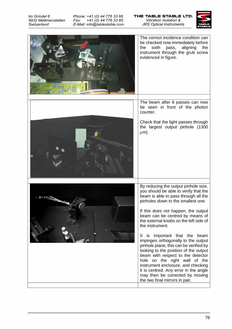
76

The correct incidence condition can be checked now immediately before the sixth pass, aligning the instrument through the grub screw evidenced in figure.

The beam after 6 passes can now be seen in front of the photon counter. Check that the light passes through the largest output pinhole (1300

m).

By reducing the output pinhole size, you should be able to verify that the beam is able to pass through all the pinholes down to the smallest one. If this does not happen, the output beam can be centred by means of the external knobs on the left side of the instrument. It is important that the beam impinges orthogonally to the output pinhole plane; this can be verified by looking to the position of the output beam with respect to the detector hole on the right wall of the instrument enclosure, and checking it is centred. Any error in the angle may then be corrected by moving the two final mirrors in pair.

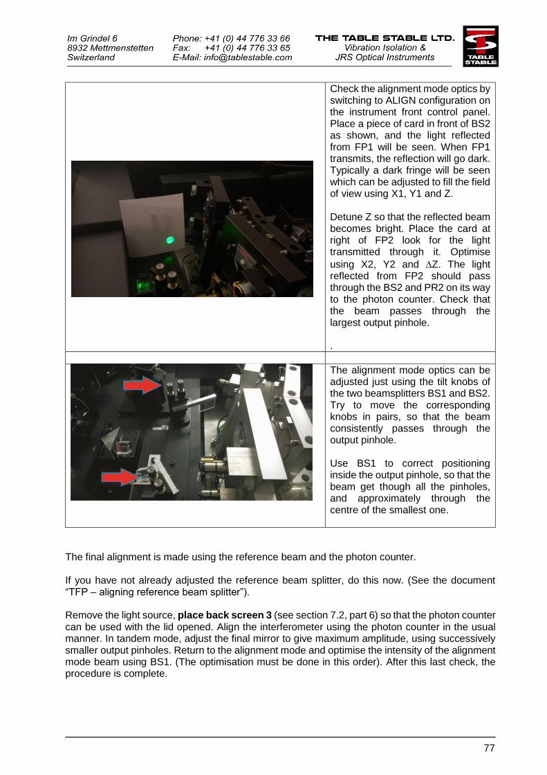
77

Check the alignment mode optics by switching to ALIGN configuration on the instrument front control panel. Place a piece of card in front of BS2 as shown, and the light reflected from FP1 will be seen. When FP1 transmits, the reflection will go dark. Typically a dark fringe will be seen which can be adjusted to fill the field of view using X1, Y1 and Z. Detune Z so that the reflected beam becomes bright. Place the card at right of FP2 look for the light transmitted through it. Optimise

using X2, Y2 and Z. The light reflected from FP2 should pass through the BS2 and PR2 on its way to the photon counter. Check that the beam passes through the largest output pinhole. .

The alignment mode optics can be adjusted just using the tilt knobs of the two beamsplitters BS1 and BS2. Try to move the corresponding knobs in pairs, so that the beam consistently passes through the output pinhole. Use BS1 to correct positioning inside the output pinhole, so that the beam get though all the pinholes, and approximately through the centre of the smallest one.

The final alignment is made using the reference beam and the photon counter. If you have not already adjusted the reference beam splitter, do this now. (See the document “TFP – aligning reference beam splitter”). Remove the light source, place back screen 3 (see section 7.2, part 6) so that the photon counter can be used with the lid opened. Align the interferometer using the photon counter in the usual manner. In tandem mode, adjust the final mirror to give maximum amplitude, using successively smaller output pinholes. Return to the alignment mode and optimise the intensity of the alignment mode beam using BS1. (The optimisation must be done in this order). After this last check, the procedure is complete.

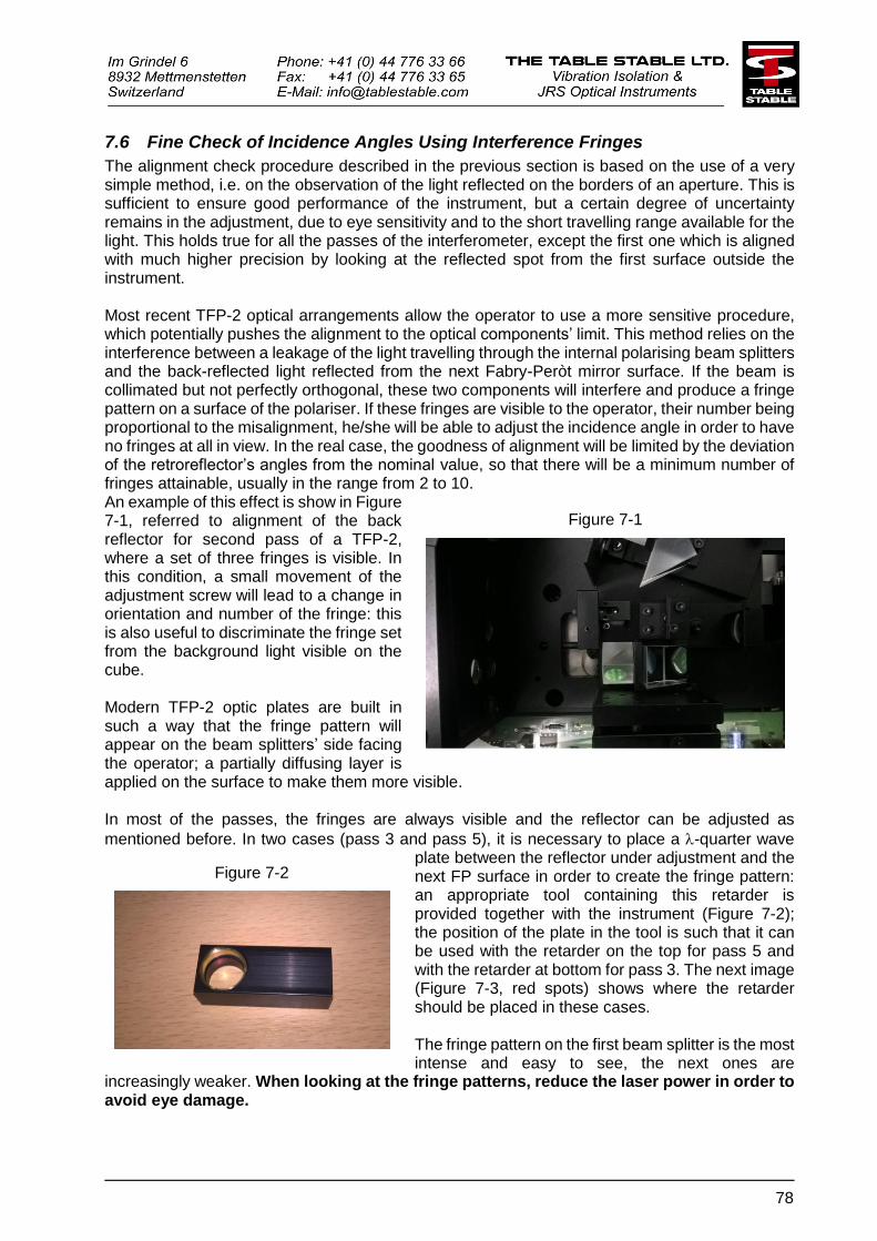
78

7.6 Fine Check of Incidence Angles Using Interference Fringes

The alignment check procedure described in the previous section is based on the use of a very simple method, i.e. on the observation of the light reflected on the borders of an aperture. This is sufficient to ensure good performance of the instrument, but a certain degree of uncertainty remains in the adjustment, due to eye sensitivity and to the short travelling range available for the light. This holds true for all the passes of the interferometer, except the first one which is aligned with much higher precision by looking at the reflected spot from the first surface outside the instrument. Most recent TFP-2 optical arrangements allow the operator to use a more sensitive procedure, which potentially pushes the alignment to the optical components’ limit. This method relies on the interference between a leakage of the light travelling through the internal polarising beam splitters and the back-reflected light reflected from the next Fabry-Peròt mirror surface. If the beam is collimated but not perfectly orthogonal, these two components will interfere and produce a fringe pattern on a surface of the polariser. If these fringes are visible to the operator, their number being proportional to the misalignment, he/she will be able to adjust the incidence angle in order to have no fringes at all in view. In the real case, the goodness of alignment will be limited by the deviation of the retroreflector’s angles from the nominal value, so that there will be a minimum number of fringes attainable, usually in the range from 2 to 10. An example of this effect is show in Figure 7-1, referred to alignment of the back reflector for second pass of a TFP-2, where a set of three fringes is visible. In this condition, a small movement of the adjustment screw will lead to a change in orientation and number of the fringe: this is also useful to discriminate the fringe set from the background light visible on the cube. Modern TFP-2 optic plates are built in such a way that the fringe pattern will appear on the beam splitters’ side facing the operator; a partially diffusing layer is applied on the surface to make them more visible. In most of the passes, the fringes are always visible and the reflector can be adjusted as

mentioned before. In two cases (pass 3 and pass 5), it is necessary to place a -quarter wave plate between the reflector under adjustment and the next FP surface in order to create the fringe pattern: an appropriate tool containing this retarder is provided together with the instrument (Figure 7-2); the position of the plate in the tool is such that it can be used with the retarder on the top for pass 5 and with the retarder at bottom for pass 3. The next image (Figure 7-3, red spots) shows where the retarder should be placed in these cases. The fringe pattern on the first beam splitter is the most intense and easy to see, the next ones are

increasingly weaker. When looking at the fringe patterns, reduce the laser power in order to avoid eye damage.

Figure 7-1

Figure 7-2

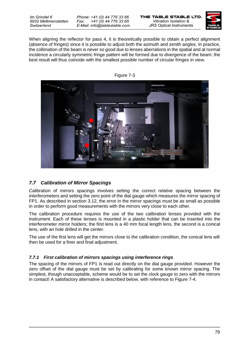
79

When aligning the reflector for pass 4, it is theoretically possible to obtain a perfect alignment (absence of fringes) since it is possible to adjust both the azimuth and zenith angles. In practice, the collimation of the beam is never so good due to lenses aberrations in the spatial and at normal incidence a circularly symmetric fringe pattern will be formed due to divergence of the beam: the best result will thus coincide with the smallest possible number of circular fringes in view.

7.7 Calibration of Mirror Spacings

Calibration of mirrors spacings involves setting the correct relative spacing between the interferometers and setting the zero point of the dial gauge which measures the mirror spacing of FP1. As described in section 3.12, the error in the mirror spacings must be as small as possible in order to perform good measurements with the mirrors very close to each other.

The calibration procedure requires the use of the two calibration lenses provided with the instrument. Each of these lenses is mounted in a plastic holder that can be inserted into the interferometer mirror holders; the first lens is a 40 mm focal length lens, the second is a conical lens, with an hole drilled in the center.

The use of the first lens will get the mirrors close to the calibration condition, the conical lens will then be used for a finer and final adjustment.

7.7.1 First calibration of mirrors spacings using interference rings

The spacing of the mirrors of FP1 is read out directly on the dial gauge provided. However the zero offset of the dial gauge must be set by calibrating for some known mirror spacing. The simplest, though unacceptable, scheme would be to set the clock gauge to zero with the mirrors in contact! A satisfactory alternative is described below, with reference to Figure 7-4.

Figure 7-3

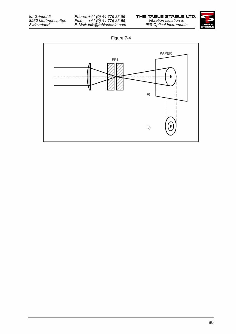
80

Figure 7-4

FP1

PAPER

a)

b)

a) Set up arbitrary spacing LA

b) Increase spacing by : LB = LA +

LB = 2LA Hence LB = 2

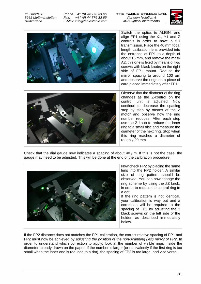
81

Switch the optics to ALIGN, and align FP1 using the X1, Y1 and Z controls in order to have a full transmission. Place the 40 mm focal length calibration lens provided into the entrance of FP1 to a depth of about 15 mm, and remove the mask A2; this one is fixed by means of two screws with black knobs on the right side of FP1 mount. Reduce the

mirror spacing to around 100 m and observe the rings on a piece of card placed immediately after FP1.

Observe that the diameter of the ring changes as the Z-control on the control unit is adjusted. Now continue to decrease the spacing step by step by means of the Z motor and observe how the ring number reduces. After each step use the Z knob to reduce the inner ring to a small disc and measure the diameter of the next ring. Stop when this ring reaches a diameter of roughly 20 mm.

Check that the dial gauge now indicates a spacing of about 40 m. If this is not the case, the gauge may need to be adjusted. This will be done at the end of the calibration procedure.

Now check FP2 by placing the same lens into the FP2 holder. A similar size of ring pattern should be observed. You can now change the

ring scheme by using the Z knob, in order to reduce the central ring to a dot. If the ring pattern is not identical, your calibration is way out and a correction will be required to the spacing of FP2 by adjusting the 3 black screws on the left side of the holder, as described immediately below.

If the FP2 distance does not matches the FP1 calibration, the correct relative spacing of FP1 and FP2 must now be achieved by adjusting the position of the non-scanning (left) mirror of FP2. In order to understand which correction to apply, look at the number of visible rings inside the diameter already drawn on the paper. If the number is larger (or equivalently if the first ring is too small when the inner one is reduced to a dot), the spacing of FP2 is too large, and vice versa.

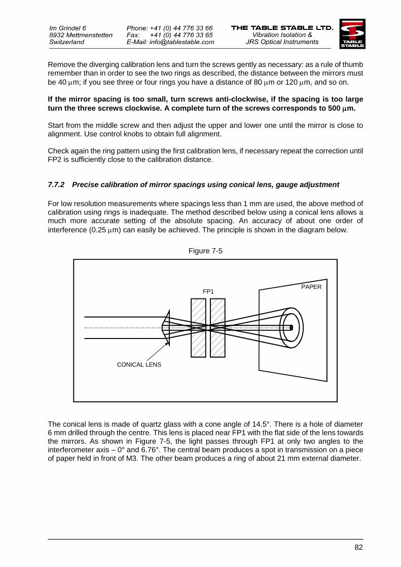
82

Remove the diverging calibration lens and turn the screws gently as necessary: as a rule of thumb remember than in order to see the two rings as described, the distance between the mirrors must

be 40 m; if you see three or four rings you have a distance of 80 m or 120 m, and so on. If the mirror spacing is too small, turn screws anti-clockwise, if the spacing is too large

turn the three screws clockwise. A complete turn of the screws corresponds to 500 m. Start from the middle screw and then adjust the upper and lower one until the mirror is close to alignment. Use control knobs to obtain full alignment. Check again the ring pattern using the first calibration lens, if necessary repeat the correction until FP2 is sufficiently close to the calibration distance.

7.7.2 Precise calibration of mirror spacings using conical lens, gauge adjustment

For low resolution measurements where spacings less than 1 mm are used, the above method of calibration using rings is inadequate. The method described below using a conical lens allows a much more accurate setting of the absolute spacing. An accuracy of about one order of

interference (0.25 m) can easily be achieved. The principle is shown in the diagram below.

Figure 7-5

FP1PAPER

CONICAL LENS

The conical lens is made of quartz glass with a cone angle of 14.5°. There is a hole of diameter 6 mm drilled through the centre. This lens is placed near FP1 with the flat side of the lens towards the mirrors. As shown in Figure 7-5, the light passes through FP1 at only two angles to the interferometer axis – 0° and 6.76°. The central beam produces a spot in transmission on a piece of paper held in front of M3. The other beam produces a ring of about 21 mm external diameter.

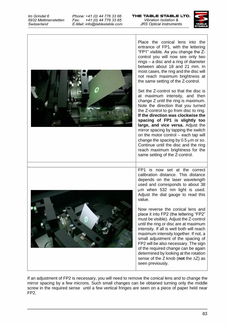
83

Place the conical lens into the entrance of FP1, with the lettering “FP1” visible. As you change the Z-control you will now see only two rings – a disc and a ring of diameter between about 18 and 21 mm. In most cases, the ring and the disc will not reach maximum brightness at the same setting of the Z-control. Set the Z-control so that the disc is at maximum intensity, and then change Z until the ring is maximum. Note the direction that you turned the Z-control to go from disc to ring. If the direction was clockwise the spacing of FP1 is slightly too large, and vice versa. Adjust the mirror spacing by tapping the switch on the motor control – each tap will

change the spacing by 0.5 m or so. Continue until the disc and the ring reach maximum brightness for the same setting of the Z-control.

FP1 is now set at the correct calibration distance. This distance depends on the laser wavelength used and corresponds to about 38

m when 532 nm light is used. Adjust the dial gauge to read this value. Now reverse the conical lens and place it into FP2 (the lettering “FP2” must be visible). Adjust the Z-control until the ring or disc are at maximum intensity. If all is well both will reach maximum intensity together. If not, a small adjustment of the spacing of FP2 will be also necessary. The sign of the required change can be again determined by looking at the rotation

sense of the Z knob (not the Z) as seen previously.

If an adjustment of FP2 is necessary, you will need to remove the conical lens and to change the mirror spacing by a few microns. Such small changes can be obtained turning only the middle screw in the required sense until a few vertical fringes are seen on a piece of paper held near FP2.

84

A fringe spacing of 1 mm corresponds to a screw movement of about 9 m. Set up the appropriate fringe spacing and then realign FP2 using only the other two screws. X2 and Y2 motors can also be used if necessary, together with knobs. After returning to full alignment, check again the calibration with the conical lens and iterate the correction if necessary. When this procedure is complete, the interferometer is fully calibrated for tandem operation at

mirror spacings greater than about 100 m. You may adjust the translation stop, see Figure 3-1, so that the minimum attainable mirror spacing

is equal to 30 m. Do not forget to replace the aperture mask A2 on the right of FP1 after completing the calibration.

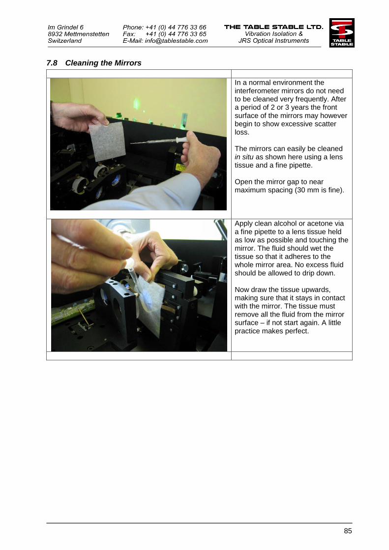
85

7.8 Cleaning the Mirrors

In a normal environment the interferometer mirrors do not need to be cleaned very frequently. After a period of 2 or 3 years the front surface of the mirrors may however begin to show excessive scatter loss. The mirrors can easily be cleaned in situ as shown here using a lens tissue and a fine pipette. Open the mirror gap to near maximum spacing (30 mm is fine).

Apply clean alcohol or acetone via a fine pipette to a lens tissue held as low as possible and touching the mirror. The fluid should wet the tissue so that it adheres to the whole mirror area. No excess fluid should be allowed to drip down. Now draw the tissue upwards, making sure that it stays in contact with the mirror. The tissue must remove all the fluid from the mirror surface – if not start again. A little practice makes perfect.

86

Notes

87