Download - Symmetry Reductions of Equations for Solute Transport in Soil

Nonlinear Dynamics22: 15–27, 2000.© 2000Kluwer Academic Publishers. Printed in the Netherlands.

Symmetry Reductions of Equations for Solute Transport in Soil

P. BROADBRIDGE, J. M. HILL, and J. M. GOARDSchool of Mathematics and Applied Statistics, University of Wollongong, Northfields Ave., Wollongong 2522,Australia

(Received: 15 March 1999; accepted: 15 April 1999)

Abstract. Solute transport in saturated soil is represented by a nonlinear system consisting of a Fokker–Planckequation coupled to Laplace’s equation. Symmetries, reductions and exact solutions are found for two dimensionaltransient solute transport through some nontrivial wedge and spiral steady water flow fields. In particular, themost general complex velocity potential is determined, such that the solute equation admits a stretching group oftransformations that would normally be possessed by a point source solution.

Keywords: Solute transport, saturated soil, dispersion, Fokker–Planck.

1. Introduction

One of the most serious environmental problems of the late 20th century is the chemicalcontamination and salinisation of soil. For example, in Australia’s Murray-Darling basin, wecan directly observe vast tracts of irrigated land that have been ruined by rising salt. Thetime scales of these regional processes is of the order of several decades. Therefore, for thepurposes of environmental management, it takes too long to experimentally determine theoutcomes of agricultural and industrial practices. Predictions must be made by mathemat-ical modelling. A full theory of solute transport will require understanding of complicatedmicroscopic processes (e.g. [1]). However coarser-scaled macroscopic models will remainimportant for economically predicting field-scale phenomena. The favoured models are sys-tems of conservation laws, expressed locally as partial differential equations for water andsolute concentrations. In practical problems, it is normal to solve these by approximate nu-merical methods. However, we face the serious problem that available numerical packageshave significant disagreement in their predictions of solute dispersion [2]. Therefore, exactsolutions are very important, not only because they provide direct unambiguous insight butalso because they are valuable bench tests for numerical schemes.

Here, we concentrate on macroscopic deterministic models based on local conservationlaws (see, e.g., [3, 4]).The solute flux densityJ is the sum of three components,

J = −2D0∇c −2De(v)∇c + cV, (1)

due to molecular diffusion, dispersion and convection respectively. The volumetric Darcianwater fluxV(r , t) is a smoothly varying representative flux, averaged over a region that islarge compared to an individual grain or pore. The dispersion term makes some allowance for

16 P. Broadbridge et al.

extra mixing within the tortuous interconnected flow paths. The dispersion coefficientDe isfound to be an increasing function of water speed, which is given byv = |V|/2, where2 isthe volumetric water concentration in the soil. In many experiments, this function is found tobe a power law,De = D1v

m, with D1 > 0 and 1≤ m ≤ 2 [5, 6]. When we combine (1) withthe mass conservation law

∂(c2)

∂t+∇.J = 0, (2)

we obtain the convection-dispersion equation,

∂(c2)

∂t= ∇.(2D(v)∇c)− ∇.(cV), (3)

whereD(v) = D0+De(v).

Most of the existing analytical solutions have assumed a uniform water flow, withV andD constant [7]. In this case, (3) reduces to the standard convection-diffusion equation withconstant coefficients. For the remainder of this article, we shall be dealing with more generaltwo-dimensional steady saturated water flows. These satisfy2 = 2s where2s is the watercontent at saturation. By Darcy’s law,V = −Ks∇φ, whereφ is the total hydraulic pressurehead andKs is the hydraulic conductivity at saturation [4, 8]. Now the equation of continuity∇.V = 0 implies Laplace’s equation

∇2φ = 0. (4)

In this case, (3) reduces to

∂c

∂t= ∇.(D(v)∇c)+ k∇φ.∇c, (5)

wherek = Ks/2s andv = |k∇φ|. Equations (4) and (5) for dependent variablesφ andc,form a nonlinear system, since the dependent variablesc andφ are coupled nonlinearly in (5).In practice, we treat (5) as a linear equation, for which (4) provides the variable coefficients.

In Section 2, we find similarity solutions for the case ofD = D0 (constant). This mayrepresent convection-diffusion in an open body of flowing liquid solvent. It may also representconvection-dispersion in soil whereinD is taken to be an average value of dispersivity. InSection 3, we consider symmetry reductions for the caseD = D1v

m. Neglect of the moleculardiffusion coefficientD0 is a common assumption since in experiments, diffusion is often aminor effect compared to dispersion.

2. Reductions for Convection-Diffusion

In a model of convection-diffusion, we assume thatD(v) in (5) is constant. Futhermore, bychoosing a length scales and a time scalets so that`2

s /ts = D, we may rescaleD to 1.Hence, we consider

∂c

∂t= ∇2c + k∇φ.∇c, (6)

together with Laplace’s equation (4). Wherever possible, it will be assumed thatk andφ havebeen rescaled so that|∇φ| is of order 1. Thencek may be interpreted as a Péclet number. Veryfew exact solutions are known, except for the case of steady unidimensional water flow,V =

Symmetry Reductions of Equations for Solute Transport in Soil17

constant. Notable exceptions are some cases with point sources of water in the plane ([6] andreferences therein), and continuous point water sources bounded within a right angled sector[10].

If we look for Lie point symmetries of the entire system (4) and (6), then we will findnothing more than rescaling ofc, translations int , and translations and rotations in(x, y).These are the only conformal maps that leave both (4) and (6) invariant. However, we mayfind symmetries that leave the single equation (6) invariant, for a given special solutionφ(x, y)

of Laplace’s equation. This may lead to useful reductions and solutions of (6) even ifφ(x, y)

is not itself an invariant solution of Laplace’s equation. For this purpose, we could carry outa symmetry classification of the single equation (6), treatingφ(x, y) as a free coefficientfunction. Given the class of functionsφ(x, y) which lead to extra symmetries, we could laterrestrict these to be solutions of Laplace’s equation. The only point symmetries for the generaldiffusion-convection equation are combinations of translations int , rescaling ofc and linearsuperposition. The symmetry generating vector fields are linear combinations of01 = ∂t ,02 = c∂c, andζ(x, y, t)∂c , wherec = ζ(x, y, t) is a general solution of the original linearequation (6). The program DIMSYM [9] finds that special cases may possibly arise when anyof the following 17 functions are linearly dependent:

φxxy φy y, φxxy φy, φxxy φx y, φxxy φx, φ2xy y, φ

2xy , φxy φy, φxy φx, φxxx φy y, φxxx φy,

φxx φy, φxxx φx y, φxxx φx, φ2xx y, φ

2xx, φxx φx, and 1.

The full classification of these special cases would be a major task and we have not completedit. Apart from the case of radial flow from a point source, which is already well known,we have found some interesting special cases which allow reduction to familiar ordinarydifferential equations.

First, for incompressible and irrotational flow with stream functionψ(x, y), we revisit thestrained flow restricted to a right angled sector,

φ = xy, ψ = (y2 − x2)/2. (7)

In this case the bounding streamlineψ = 0 is piecewise linear, with polar anglesθ =±π/4. Then the finite part (excluding linear superposition) of the Lie algebra of infinitesimalpoint symmetry generators is nine dimensional, compared to two dimensional in the genericcase. The additional basis vectors of the symmetry algebra may be chosen to be

03 = kψ(x, y)c∂c + ∂θ where ∂θ = x∂y − y∂x,

04 = e−kt[ck

2(x − y)∂c + ∂x

],

05 = e−kt[−ck

2(x − y)∂c + ∂y

],

06 = ekt [−ck(x + y)∂c + 2∂x],07 = ekt [−ck(x + y)∂c + 2∂y],

08 = e2kt

[kx∂x + ky∂y + ∂t −

[k2c

2(x2+ y2)+ k2xyc + kc

]∂c

],

09 = e−2kt

[−kx∂x − ky∂y + ∂t −

[k2c

2(x2+ y2)− k2xyc − kc

]∂c

].


A wide variety of symmetry reductions is possible. In particular, we have found that03

leads to explicit solutions satisfying standard boundary conditions. These invariant solutionsare of the form

c = e−(1/2)kxyF (R, t), (8)

whereR denotesr2 = x2 + y2, andF satisfies

4RFRR + 4FR − k2R

4F = Ft . (9)

At the boundary streamlines, there is no normal convection and neither is there normaldiffusion, since it is clear from (8) that withθ = tan−1(y/x), ∂c/∂θ = 0 at θ = ±π/4.Hence, we automatically satisfy the physical boundary conditions that both water and soluteare contained within the bounds of the wedge.

If we apply the additional boundary conditions thatF(R) is analytic asR→ 0 andF → 0asR → ∞, as well as general initial conditionF = g(kR/2), then we obtain the seriessolution

F =∞∑n=1

Bn e−λnt−kR/4Ln(kR/2), (10)

whereλn = (2n+ 1)k, Ln is thenth Laguerre polynomial, and

Bn = ∞∫

0

e−u/2Ln(u)g(u) du

/ ∞∫0

e−u(Ln(u))2 du

.We have constructed the smooth solution with initial conditionF = 1 for r < 0.2 and

F = 0 for r > 0.2. As expected, the solute concentration contours spread diffusively in analmost circular fashion at early timest < 0.1 but at later times they are elongated along thedominant direction of water flow ,θ = −π/4. The continuous solute line source solutionfor this problem was given by Maas [10] and the instantaneous source solution was given byZoppou and Knight [11]. These solutions could be used as Green’s functions in an alternativeapproach to the solution of initial value problems and boundary-initial problems.

We can also solve boundary value problems on the finite region(r, θ) ∈ [ε,A] ×[−π/4, π/4]. Consider the boundary conditions

F(ε2) = γ, F (A2) = 0,

as well as the previously mentioned no-flow conditions atθ = ±π/4. By (8), this correspondsto almost uniform concentrationc at a thin circular discharge piper = ε, and completeremoval of solute (c = 0) at an outer surfacer = A. The steady state solution satisfies

R2F ′′(R)+ RF ′(R)− k2

16R2F = 0. (11)

It follows that the steady solution satisfying the prescribed boundary conditions is

F∞(R) = C1I0(kR/4)+ C2K0(kR/4), (12)


whereI0 andK0 are the modified Bessel functions of order zero,

C1 = γ I0(kA2/4)

I0(kA2/4)K0(kε2/4)− I0(kε2/4)K0(kA2/4),

C2 = −γK0(kA2/4)

I0(kA2/4)K0(kε2/4)− I0(kε2/4)K0(kA2/4).

Now we solve for the transientF(R, t) = F(R, t)− F∞(R), which now satisfies a linearequation (9), as well as homogeneous boundary conditionsF = 0 atR = ε2, A2. Using theseparation of variables technique, we obtain the solution

F =∞∑n=1

Bn e−λnt−kR/4Fn(kR/2),

Fn(u) = M(µn,1, u)− U(µn,1, u)M(µn,1, kε2/2)/U(µn,1, kε2/2), (13)

whereM(a, b, c) andU(a, b, c) are the standard confluent hypergeometric functions (see[12, p. 504]) and the eigenvaluesµn = [1− λn/k]/2 are the solutions of the equation

M(µ,1, kε2/2)U(µ,1, kA2/2)− U(µ,1, kε2/2)M(µ,1, kA2/2) = 0. (14)

The series coefficients are given by

Bi =kA2/2∫kε2/2

g(2u/k)Fi(u)e−u du/

kA2/2∫kε2/2

Fi(u)2 e−u du, (15)

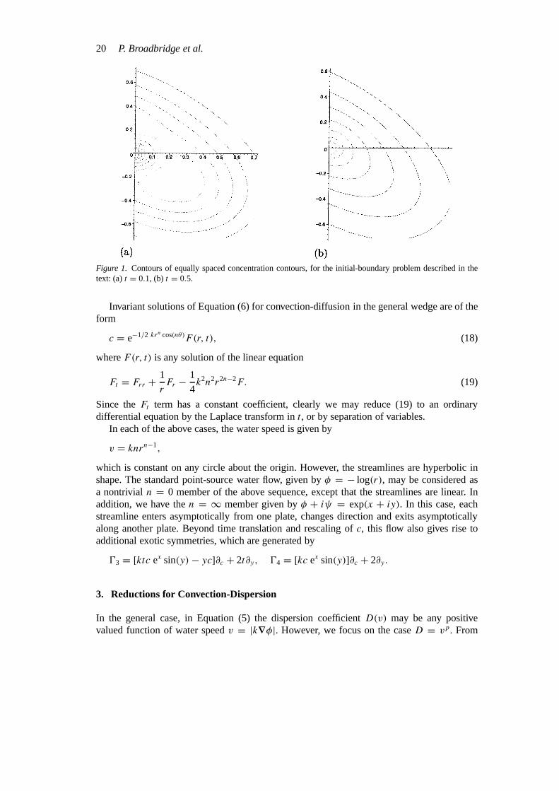
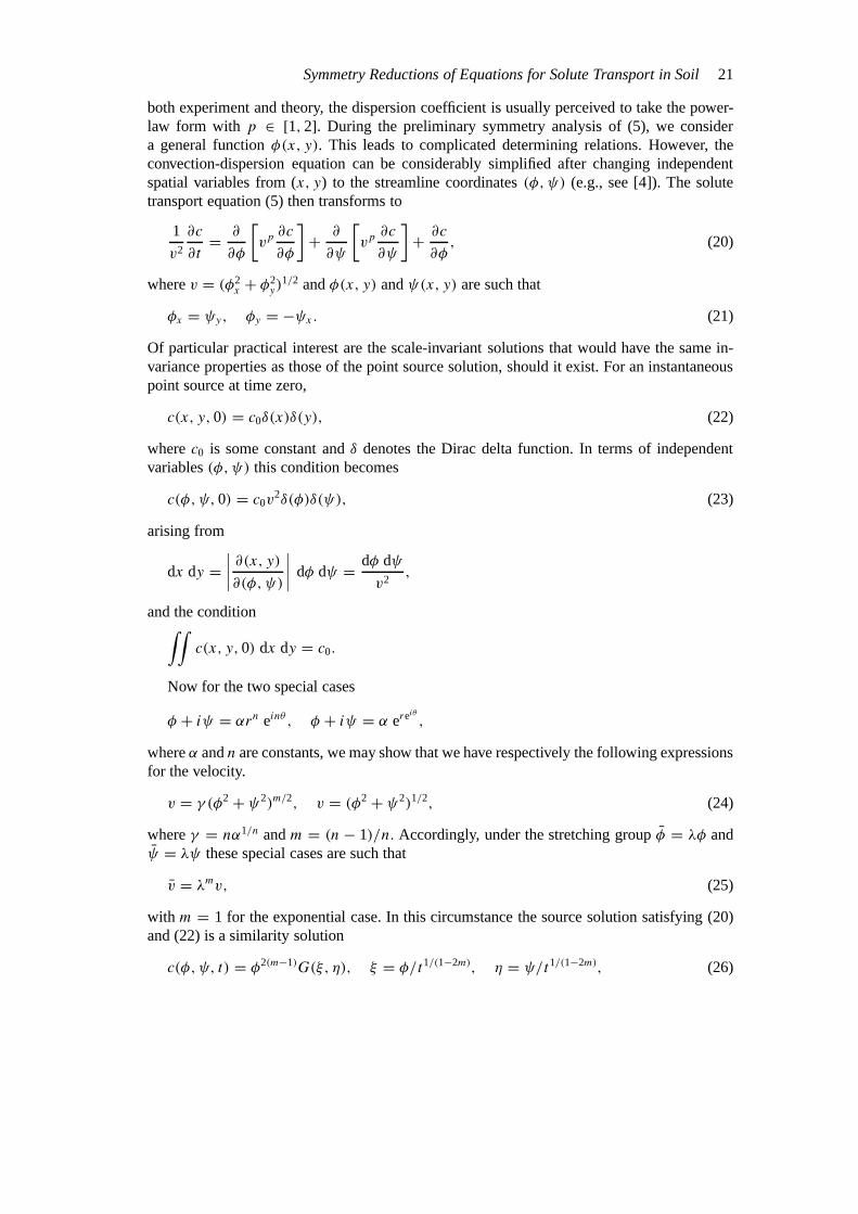
whereg(R) is the initial value forF (R).Figure 1 displays the solute contours, plotted by MAPLE [13], for the case ofε = 0.05,

γ = 1, k = 10 andA = 1, with initial conditiong(R) = −55k2(R − ε2)(R − A2).Note that neither water nor solute flows across the bounding streamlines at polar angles

θ = ±π/4,±3π/4. We are principally interested in the sectorθ ∈ [−π/4, π/4]. However,the solute concentration contours may be extended smoothly and asymmetrically into theneighbouring sectors, wherein other solutions may be constructed from the series (13). Fromthe boundary conditions, the outer contour must be the circler = A. The figure displays theinterior regionr < 0.7, wherein the initial condition is highly irregular. Since the smoothsteady state solution is stable, information on the initial condition will eventually be washedaway. With this high value of Péclet number, the initial irregularity is still evident at timet = 0.1 even though the contours have been elongated in the direction of the water flow. Attime t = 0.5, the contours show little evidence of the initial conditions.

For a water flow constrained to a more general wedge sectorθ ∈ [0, π/n], with n 6= 0 thecomplex velocity potential is

ω = φ + iψ = (x + iy)n, (16)

and in this case, Equation (6) still has the symmetry generator

03 = 1

2nkψ(x, y)c∂c + ∂θ . (17)


Figure 1. Contours of equally spaced concentration contours, for the initial-boundary problem described in thetext: (a)t = 0.1, (b) t = 0.5.

Invariant solutions of Equation (6) for convection-diffusion in the general wedge are of theform

c = e−1/2 krn cos(nθ)F (r, t), (18)

whereF(r, t) is any solution of the linear equation

Ft = Frr + 1

rFr − 1

4k2n2r2n−2F. (19)

Since theFt term has a constant coefficient, clearly we may reduce (19) to an ordinarydifferential equation by the Laplace transform int , or by separation of variables.

In each of the above cases, the water speed is given by

v = knrn−1,

which is constant on any circle about the origin. However, the streamlines are hyperbolic inshape. The standard point-source water flow, given byφ = − log(r), may be considered asa nontrivialn = 0 member of the above sequence, except that the streamlines are linear. Inaddition, we have then = ∞ member given byφ + iψ = exp(x + iy). In this case, eachstreamline enters asymptotically from one plate, changes direction and exits asymptoticallyalong another plate. Beyond time translation and rescaling ofc, this flow also gives rise toadditional exotic symmetries, which are generated by

03 = [ktc ex sin(y)− yc]∂c + 2t∂y, 04 = [kc ex sin(y)]∂c + 2∂y.

3. Reductions for Convection-Dispersion

In the general case, in Equation (5) the dispersion coefficientD(v) may be any positivevalued function of water speedv = |k∇φ|. However, we focus on the caseD = vp. From


both experiment and theory, the dispersion coefficient is usually perceived to take the power-law form with p ∈ [1,2]. During the preliminary symmetry analysis of (5), we considera general functionφ(x, y). This leads to complicated determining relations. However, theconvection-dispersion equation can be considerably simplified after changing independentspatial variables from (x, y) to the streamline coordinates(φ,ψ) (e.g., see [4]). The solutetransport equation (5) then transforms to

1

v2

∂c

∂t= ∂

∂φ

[vp∂c

∂φ

]+ ∂

∂ψ

[vp∂c

∂ψ

]+ ∂c

∂φ, (20)

wherev = (φ2x + φ2

y)1/2 andφ(x, y) andψ(x, y) are such that

φx = ψy, φy = −ψx. (21)

Of particular practical interest are the scale-invariant solutions that would have the same in-variance properties as those of the point source solution, should it exist. For an instantaneouspoint source at time zero,

c(x, y,0) = c0δ(x)δ(y), (22)

wherec0 is some constant andδ denotes the Dirac delta function. In terms of independentvariables(φ,ψ) this condition becomes

c(φ,ψ,0) = c0v2δ(φ)δ(ψ), (23)

arising from

dx dy =∣∣∣∣ ∂(x, y)∂(φ,ψ)

∣∣∣∣ dφ dψ = dφ dψ

v2,

and the condition∫∫c(x, y,0) dx dy = c0.

Now for the two special cases

φ + iψ = αrn einθ , φ + iψ = α ereiθ

,

whereα andn are constants, we may show that we have respectively the following expressionsfor the velocity.

v = γ (φ2+ ψ2)m/2, v = (φ2+ ψ2)1/2, (24)

whereγ = nα1/n andm = (n − 1)/n. Accordingly, under the stretching groupφ = λφ andψ = λψ these special cases are such that

v = λmv, (25)

with m = 1 for the exponential case. In this circumstance the source solution satisfying (20)and (22) is a similarity solution

c(φ,ψ, t) = φ2(m−1)G(ξ, η), ξ = φ/t1/(1−2m), η = ψ/t1/(1−2m), (26)


where we have usedδ(λφ) = λ−1δ(φ) and on assumingt = λδt we have from (20), (23) and(25) the constraints

δ = 1− 2m p = 1/m.

We note that in the special casem = 1/2, t is an invariant and the similarity solution (26)takes the form

c(φ,ψ, t) = φ−1G(ξ, t), ξ = φ/ψ. (27)

Thus, form 6= 1/2 and assumingv is given by (24)1 we obtain from (20) and (26) the linearpartial differential equation in two independent variables

γ 1/m(1+ η2/ξ2)m+1/2[ξ2(Gξξ +Gηη)+ 4(m− 1)ξGξ + 2(m− 1)(2m− 3)G]+ γ 1/m(1+ η2/ξ2)m−1/2[ξGξ + ηGη + 2(m− 1)G] + (1+ η2/ξ2)m

× [ξGξ + 2(m− 1)G] + ξ1−2m

γ 2(1− 2m)(ξGξ + ηGη) = 0, (28)

which admits a number of special simple cases such asm = 1.Similarly form = 1/2 and assumingv is given by (24)2 we have from (20) and (26)

Gt

γ 2+ γ 2G = γ 2(1+ ξ2)

d

dξ

{(1+ ξ2)Gξ − 2G

ξ

}+ (1+ ξ2)1/2

(Gξ − G

ξ

), (29)

which simplifies somewhat in terms of the variable tan−1(ξ). The solutions of these linearequations will be examined in detail elsewhere.

Given the usefulness of the above reductions it is natural to ask the question as to whetherwe might be able to determine the most general harmonicφ + iψ such thatv = (φ2

x + φ2y)

1/2

satisfies (25) under the stretching group of transformations. In other words can we determinethe most generalφ + iψ such that

v = φmf (φ/ψ), (30)

for some functionf ? As sketched in Appendix A we show that the most general complexpotentialφ + iψ is given by

φ + iψ = (α + iβ)(x + iy)a+ib, (31)

and thatf (ξ), whereξ here denotesφ/ψ , is given explicitly by

f (ξ) = (1+ ξ2)m/2

ξmAeB tan−1(ξ), (32)

whereα, β, a, b andA andB designate certain arbitrary constants.Equation (20) is amenable to symmetry analysis but a full classification has not yet been

completed. With the aid of DIMSYM [9], it becomes clear that the symmetry determiningrelations may give additional symmetries whenvφ = 0 or when either of the following issatisfied:

∂φ{λ(λφφ + λψψ)− (λ2

φ + λ2ψ)} = 0, ∂ψ

{λ(λφφ + λψψ)− (λ2

φ + λ2ψ)} = 0, (33)


whereλ = v2. Even after solving each of the above three equations for special casesv(φ,ψ),we must further restrict these cases so that they are compatible with the conditions (21) forincompressible irrotational flow. As briefly shown in Appendix B the conditionvφ = 0 ismore amenable but it leads only to the point vortex flow which is conjugate to the previouslystudied case of the point source flow.

In all of the scale-invariant forms of the convection-dispersion equation considered above,both conditions (33) are satisfied by taking

λ(λφφ + λψψ)− (λ2φ + λ2

ψ) = 0, (34)

which is equivalent to Laplace’s equation

µφφ + µψψ = 0, (35)

whereµ = log(λ) = 2 log(v). Finally, we comment on the interesting possibility that (33)may also be satisfied by replacing the right hand side of (34) by a nonzero constantD. In thiscase,µ satisfies the Liouville equation

µφφ + µψψ = D e−2µ, (36)

which itself transforms to the Laplace equation by a Bäcklund transformation [14]. We havenot yet investigated whether nontrivial solutions of Liouville’s equation, or more generally,nontrivial solutions of (33), satisfying

λ(λφφ + λψψ)− (λ2φ + λ2

ψ) = h(ψ),with h′ 6= 0, do in fact lead to additional symmetries for solute convection-dispersion.

4. Conclusion

A Lie point symmetry analysis of the equations for two-dimensional solute transport in soil,results in a rich class of symmetries for a number of practically important background waterflow fields. For transient solute diffusion-convection, steady wedge flows allow symmetryreductions that are compatible with zero solute flux at the wedge boundaries. This allowsreduction to relatively simple linear second order ordinary differential equations.

For transient solute dispersion-convection, we have determined the most general complexvelocity potentialφ + iψ such that the solute equation admits the simple stretching group oftransformations normally associated with a point source solution.The resulting linear partialdifferential equations will be examined in detail elsewhere.

A full symmetry classification is yet to be achieved. However we have already presentedsome physically appealing reductions and explicit solutions.

Acknowledgement

James M. Hill is grateful to the Australian Research Council for providing a Senior ResearchFellowship.


Appendix A: Most General φ + iψ Such That v= φmf (φ/ψ)

Sincev = (φ2x + φ2

y)1/2, in this case we may introducew(x, y) such that

φx = φmf (ξ) cosw, φy = φmf (ξ) sinw, (A.1)

where here,ξ = φ/ψ. Now by compatibility and using the Cauchy–Riemann equations (21)we may eventually deduce

wx = φm−1[(ξf ′ +mf ) sinw − ξ2f ′ cosw],wy = −φm−1[(ξf ′ +mf ) cosw + ξ2f ′ sinw], (A.2)

where primes denote differentiation with respect toξ . From the compatibility ofw(x, y) weobtain

f [ξ(ξf ′ +mf )′ + (m− 1)(ξf ′ +mf )] + ξ2f (ξ2f ′)′ = (ξf ′ +mf )2+ (ξ2f ′)2, (A.3)

which may be considerably simplified to yield

ξ2(1+ ξ2)(ff ′′ − f ′2)+ 2ξ3ff ′ = mf 2. (A.4)

On dividing this equation byf 2 we obtain a simple first order ordinary differential equationfor f ′/f which may be readily integrated twice to yieldf (ξ) given by (32) in terms of twoarbitrary constantsA andB.

Now on eliminating the sines and cosines from (A2) by means of the relations (A1) weobtain

wx = mφyφ+ g(ξ)ξy, wy = −mφx

φ− g(ξ)ξx,

whereg(ξ) = f ′/f is given by

g(ξ) = − m

ξ(1+ ξ2)+ B

(1+ ξ2).

Thus, these equations can be re-formulated as

wx = (m logφ + logf )y, wy = −(m logφ + logf )x,

and therefore from Equation (30) we have

wx = (logv)y wy = −(logv)x, (A.5)

from which we deduce thatw + i log v is an analytic function ofx + iy. From (30) and (32)we find

v = A(φ2+ ψ2)m/2 eB tan−1(φ/ψ),

and this equation combined with (21) and (A5) yields an integration

w = m tan−1

(φ

ψ

)− B

2log(φ2+ ψ2)+ w0, (A.6)


wherew0 denotes an arbitrary constant. Finally, from (32), (A1) and (A6) we may deduce theequation

ζz = A∗ζm+iB, (A.7)

whereζ = φ + iψ , A∗ = A e−i(m+iB)π/2 and we have utilized the well known relation forinverse tangents

tan−1(z)+ tan−1

(1

z

)= π

2.

It is clear from (A7) thatζ = φ + iψ has the structure (31) for certain real constantsα, β, a

andb.Alternatively, starting from (31) it is not difficult to show that

φ2+ ψ2 = (α2+ β2)r2a e−2bθ , tan−1(ψ/φ) = aθ + b log r + d, (A.8)

whered denotes tan−1(β/α), r = (x2 + y2)1/2 andθ = tan−1(y/x). Further, we have

v2 = φ2r +

φ2θ

r2= (α2+ β2)(a2+ b2)r2(a−1) e−2bθ , (A.9)

and therefore by elimination ofr andθ from (A8) we obtain

v2 = (a2+ b2)(α2+ β2)a/(a2+b2)(φ2+ ψ2)1−(a/(a

2+b2)) e(2b/(a2+b2))[tan−1(φ/ψ)−tan−1(α/β)] (A.10)

which coincides with that given by (30) and (32) where the constantsA andB andm are givenby

A = (a2+ b2)1/2(α2+ β2)a/2(a2+b2) e−(2b tan−1(α/β)/(a2+b2)),

B = b

(a2+ b2), m = 1− a

(a2 + b2). (A.11)

Appendix B: Most General φ + iψ Such Thatv = f (ψ)

In order to solve

ψ2x + ψ2

y = f (ψ)2, ψxx + ψyy = 0, (B.1)

we introducew(x, y) such that

ψx = f (ψ) cosw, ψy = f (ψ) sinw.

Then from the compatibility and (B1)2 we obtain

wx = f ′ sinw, wy = −f ′ cosw, (B.2)

where primes here denote differentiation with respect toψ . Compatibility forw givesff ′′ =f ′2, which may be readily integrated to yield

f (ψ) = A eBψ, (B.3)


whereA andB denote arbitrary constants. From the above relations we may deduce thatw + iBψ is an analytic function ofx + iy and thereforew(x, y) = Bφ(x, y) so that (B2)becomes

ψx = A eBψ cosBφ, ψy = A eBψ sinBφ. (B.4)

From these equationsζ = φ − iψ satisfies

ζz = −iAeiBζ ,

which on integration gives

ζ = i

BlogAB(z0− z), (B.5)

wherez0 denotes an arbitrary complex number. From (B5) we obtain

φ(x, y) = −1

Btan−1

(y − y0

x − x0

),

ψ(x, y) = −1

Blog

(AB[(x − x0)

2+ (y − y0)2]1/2) . (B.6)

This results in

v = A eBψ = 1

B[(x − x0)2+ (y − y0)2]1/2 ,

which, apart from arbitrary translational constants, corresponds to point vortex flow.

References

1. Jury, W. A., ‘Solute transport and dispersion’, inFlow and Transport in the Natural Environment: Advancesand Applications, W. L. Steffen and O. T. Denmead (eds.), Springer-Verlag, Berlin, 1988, pp. 1–16.

2. Woods, J., Simmons, C. T., and Narayan, K. A., ‘Verification of black box groundwater models’, inEMAC98Proceedings of the Third Biennial Engineering Mathematics and Applications Conference, E. O. Tuck andJ. A. K. Stott (eds.), Institution of Engineers Australia, Adelaide, 1998, pp. 523–526.

3. Wierenga, P. J., ‘Water and solute transport and storage’, inHandbook of Vadose Zone Characterization andMonitoring, L. G. Wilson, G. E. Lorne, and S. J. Cullen (eds.), Lewis Publishers, Boca Raton, FL, 1995,pp. 41–60.

4. Ségol, G.,Classic Groundwater Simulations: Proving and Improving Numerical Models, Prentice Hall,Englewood Cliffs, NJ, 1994.

5. Salles, J., Thovert, J.-F., Delannay, R., Presons, L., Auriault, J.-L., and Adler, P. M., ‘Taylor dispersion inporous media: Determination of the dispersion tensor’,Physics of Fluids A5, 1993, 2348–2376.

6. Philip, J. R., ‘Some exact solutions of convection-diffusion and diffusion equations’,Water ResourcesResearch30, 1994, 3545–3551.

7. van Genuchten, M. T. and Alves, W. J., ‘Analytical solutions of the one-dimensional convective-dispersivesolute transport equation’,U.S. Department of Agriculture, Technical Bulletin1661, 1982, 1–151.

8. Philip, J. R., ‘Theory of infiltration’,Advances in Hydrosciences5, 1969, 215–296.9. Sherring, J., ‘DIMSYM: Symmetry determination and linear differential equations package’, Research

Report, Latrobe University Mathematics Department, 1993, http://www.latrobe.edu.au/www/mathstats/Maths/Dimsym/

10. Maas, L. R. M., ‘A closed form Green function describing diffusion in a strained flow field’,SIAM Journalof Applied Mathematics49, 1989, 1359–1373.


11. Zoppou, C. and Knight, J. H., ‘Analytical solution of a spatially variable coefficient advection-diffusionequation in one-, two- and three-dimensions’, Preprint, CSIRO, Land and Water, Canberra, 1998.

12. Abramowitz, M. and Stegun, I. A. (eds.),Handbook of Mathematical Functions, Dover, New York, 1972.13. Redfern, D.,The Maple Handbook, Springer-Verlag, New York, 1996.14. Ibragimov, N. H. (ed.)CRC Handbook of Lie Group Analysis of Differential Equations, Vol. 2, Sec-

tion 8.12.1, CRC Press, Boca Raton, FL, 1996.

Download - Symmetry Reductions of Equations for Solute Transport in Soil

Top Related