Silvina Rybnikov Supervisors: Prof. Ilan Shimshoni and Prof. Ehud Rivlin

HomePage: http://www.cs.technion.ac.il/~silvina

Introduction◦ Problem statement◦ Existing research◦ Thesis goals◦ The robot

Algorithm outline Navigation to a single target Single image cover Room estimation Room coverage Improving positioning Algorithm Experiment

AGVs can be used in:◦ Industrial applications to move materials around

a manufacturing facility or a warehouse.◦ Storage◦ Delivery◦ Transport

medicine in hospitals

◦ Transporting containers in ports

Easy navigation from an unknown position to predefined targets.

No human intervention. No artificial beacons/landmarks.

Reliable representation of targets◦ Minimum probability of misidentification.◦ Robust to small changes in the environment.◦ A good solution is an image taken from the target

pose Autonomous environment exploration

◦ Find all targets. A representation of targets relative

positions ◦ Support easy navigation to a required target from

an unknown position.

SLAM (Simultaneous Localization And Map Building)◦ Collect all the features into a map of the explored

environment.◦ Next week in pixel club : "Visual Simultaneous

Localization and Mapping using Inverse Scaling Parametrization and Uncertain Projective Geometry", Dr. Davide Migliore

Path Following◦ A human operator steers the robot on a

path/paths while capturing images after each small step.

◦ The robot can repeat the same path or reach a goal near the graph of paths.

Build a robotic system with an efficient algorithm for targets search.

Find ways to improve positioning accuracy. Implement the entire robotic system which:

◦ explores the environment◦ locates the targets ◦ builds a representation of targets relative

position◦ enables navigation from any position to any

target

Robot equipped with a single camera◦ The camera is stationary

Robot moves only on a plane (X-Z plane)

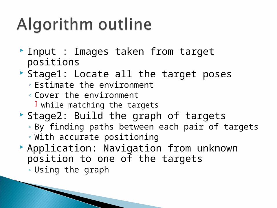
Input : Images taken from target positions Stage1: Locate all the target poses

◦ Estimate the environment◦ Cover the environment

while matching the targets Stage2: Build the graph of targets

◦ By finding paths between each pair of targets◦ With accurate positioning

Application: Navigation from unknown position to one of the targets ◦ Using the graph

Algorithm for reaching a position described by an image ◦ Appears in “Image-Based Robot Navigation in

Unknown Indoor Environments” by E. Rivlin, I.Shimshoni , and E. Smolyar.

Algorithm has two stages called iteratively:◦ Finding direction to the target◦ Finding the distance to the target

Given two images which partially overlap we can find :◦ Direction between the cameras centers◦ Rotation between the cameras view directions

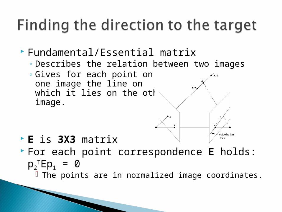
Fundamental/Essential matrix◦ Describes the relation between two images◦ Gives for each point on

one image the line on which it lies on the other image.

E is 3X3 matrix For each point correspondence E holds:

p2TEp1 = 0 The points are in normalized image coordinates.

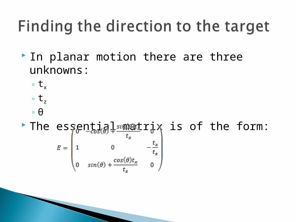
In planar motion there are three unknowns:◦ tx

◦ tz

◦ θ The essential matrix is of the form:

A linear solution requires 3 point correspondences.

We use the linear solution as a starting point for a non linear optimization with two unknowns : ◦ tx /tz

◦ θ

Since there are outliers in the SIFT matching process we use PROSAC to select triplets for the Essential matrix calculation.◦ PROSAC (Progressive Sample Consensus) is a variant of

RANSAC (Random Sample Consensus)

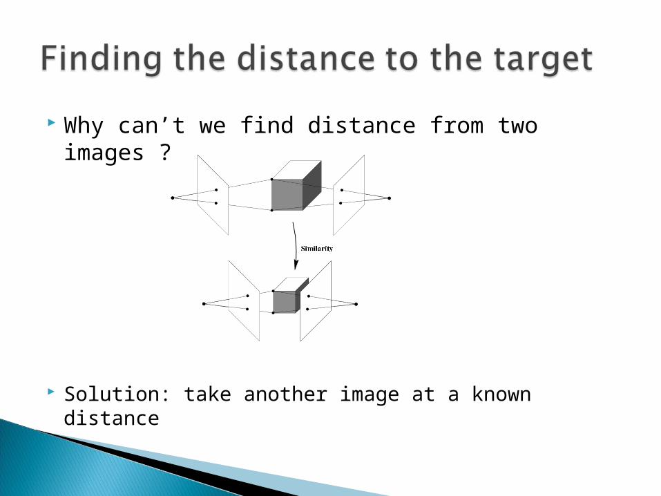
Why can’t we find distance from two images ?

Solution: take another image at a known distance

The robot moves in direction tx /tz a step of length λ. Features are matched in the three images The distance remaining to the target can be

calculated from each triplet of correspondences after removing the difference in rotations.

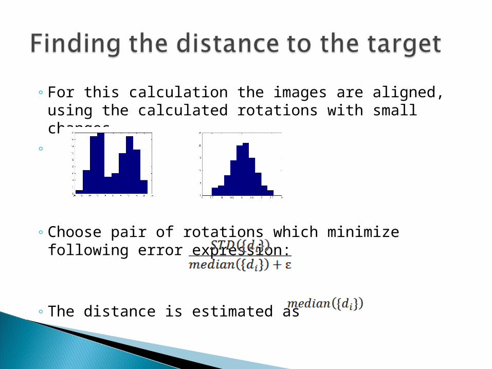
◦ For this calculation the images are aligned, using the calculated rotations with small changes.

◦

◦ Choose pair of rotations which minimize following error expression:

◦ The distance is estimated as

Introduction◦ Problem statement◦ Existing research◦ Thesis goals◦ The robot

Algorithm outline Navigation to a single target Single image cover Room estimation Room coverage Improving positioning Algorithm Experiment

Configuration space of the robot is the set of all possible positions (x,z) and orientations θ.

How much of the configuration space a single image covers ?

◦ The covered space is the positions and orientations in which an image taken will match the current image.

We have estimated the covered space experimentally.

The size of the covered space depends on the distance from the viewed scene, we claim that the dependence is linear.

The resulting shape can be resized according to the distance from the scene.

The coverage has three scores :1.No - very low probability of a match 2.Maybe - some probability of a match3.Yes - very high probability of a match

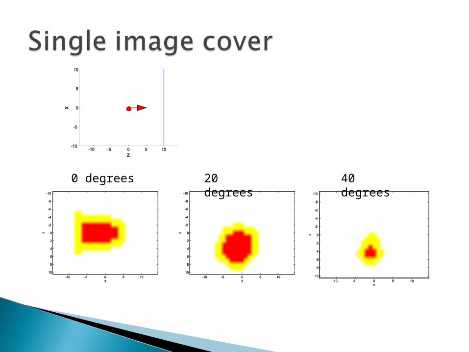
0 degrees 20 degrees

40 degrees

Why ?1. The space for coverage.2. The size of a SIC of an image taken at a specific

pose. How ?

◦ 12 stereo pairs

◦ In each pair SIFT features are matched (along the epipolar line) and their 3D position recovered.

The features above the floor and below 2 meters are considered as obsticles.

The walls are estimated from those features.

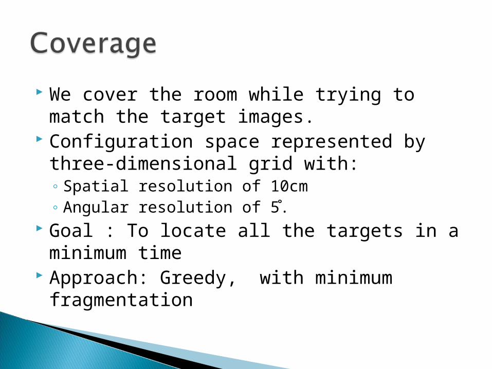
We cover the room while trying to match the target images.

Configuration space represented by three-dimensional grid with:◦ Spatial resolution of 10cm ◦ Angular resolution of 5 ̊.

Goal : To locate all the targets in a minimum time Approach: Greedy, with minimum fragmentation

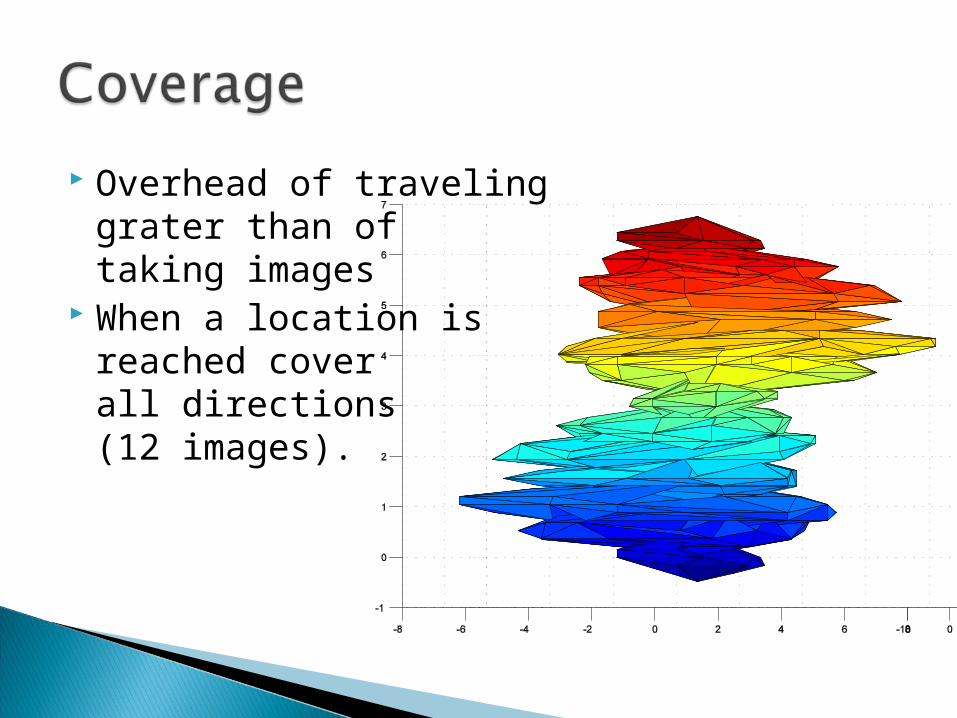
Overhead of traveling grater than oftaking images When a location isreached cover all directions (12 images).

Minimize fragmentation by encouraging overlap in the Maybe portions of the SICs.

Two overlapping Maybe scores considered as a Yes score.

Score for position : the additional Yes volume added by the 12 SICs.

Precompute SICs at different scales and orientations

Greedy approach (no lookahead) Score computations only for points on a

random greed. Out of the possible 6 angle offsets only two

are checked: 0 and 15

Errors in odometry propagate and increase. We choose a reference pose during the

room estimation stage.◦ The pose is saved as an image taken from it

The robot returns after each exploration to the reference pose.

We use EKF (Extended Kalman Filter) ◦ module the current pose covariance◦ Improve pose estimation with two kinds of

observations

The Kalman filter is a recursive estimator.◦ Only the estimated state from the previous time

step and the current measurement are needed to compute the estimate for the current state.

The Kalman filter has two distinct phases: Predict and Update.◦ Predict: Make a step from the previous estimated

state.◦ Update: Use observations to update the predicted

state.

The robot rotates β radians and travels d cm. α is the orientation after the rotation by β.

G - Jacobian matrix of the partial derivatives of the update function of P with respect to P

V - Jacobian matrix of the partial derivatives of the update function of P with respect to (d, β)

M- the covariance of the step

When a target image is first matched, its matching image J is saved. PJ and ΣJ are also saved.◦ From then on the covariance is calculated relative to PJ.

When the target pose is reached, the pose PT is improved by finding the angle θ between the current image and image J.

The path back from the target to the reference pose is used as an observation to improve the estimate of the target pose.

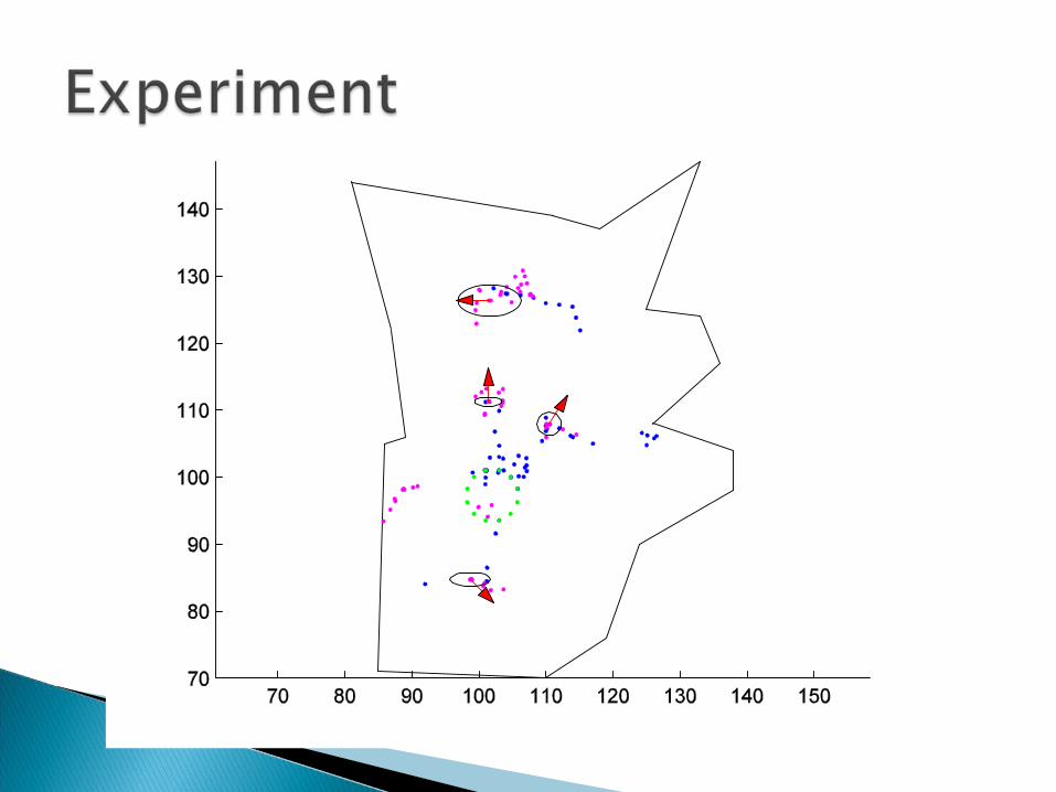
Estimate room Locate the targets

◦ The search is driven by the goal to cover the search space with a minimum number of movements and images.

◦ After each exploration the robot returns to the reference pose.

Connect all the pairs of targets by an edge◦ In case of failure to go between two targets return

to reference pose. ◦ Edge estimated from both the way forth and back

Estimates are combined using EKF (observation II)

Navigation from unknown position◦ Robot receives an identifier of a target to go to◦ Robot rotates on a spot till one of the targets in

the graph is matched◦ If no target matched makes a random move and

repeats the previous step◦ Finds the path with the lowest cost on the graph

from the current node to the requested node. The cost is the sum of the uncertainties on the

edges.◦ Follows the path

experiment1.mp4

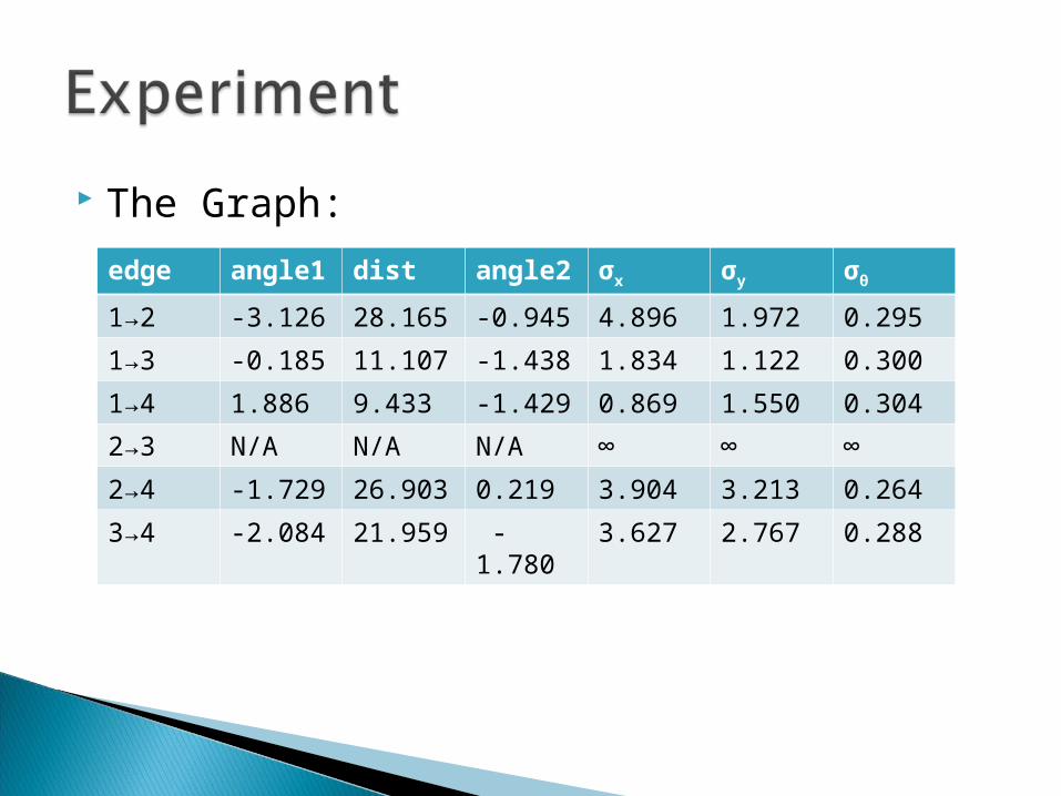
The Graph:

edge angle1 dist angle2 σx σy σθ

1→2 -3.126 28.165 -0.945 4.896 1.972 0.295

1→3 -0.185 11.107 -1.438 1.834 1.122 0.300

1→4 1.886 9.433 -1.429 0.869 1.550 0.304

2→3 N/A N/A N/A ∞ ∞ ∞

2→4 -1.729 26.903 0.219 3.904 3.213 0.264

3→4 -2.084 21.959 -1.780 3.627 2.767 0.288