Short-term meso-scale variability of mesozooplankton communities in a coastal
upwelling system (NW Spain)
1
2
3
4 5
6
7
Álvaro Rouraa*, Xosé A. Álvarez-Salgadoa, Ángel F. Gonzáleza, María Gregoria,
Gabriel Rosónb, Ángel Guerraa a IIM-CSIC, Instituto de Investigaciones Marinas, 36208 Vigo, Spain TEL: (+34) 986 231 930. FAX:
(+34) 986 292762
b GOFUVI, Facultad de Ciencias del Mar, Universidad de Vigo, 36200 Vigo, Pontevedra, Spain
*Corresponding author: [email protected], IIM-CSIC, Instituto de Investigaciones Marinas, 36208
Vigo, Spain TEL: (+34) 986 231 930. FAX: (+34) 986 292762.
8
9
10
11
12
13
14
15
16
17
18
19
20
21
22
23
24
25
26
27
28
29
30
31
32
Abstract
The short-term, meso-scale variability of the mesozooplankton community present in
the coastal upwelling system of the Ría de Vigo (NW Spain) has been analysed. Three
well-defined communities were identified: coastal, frontal and oceanic, according to
their holoplankton-meroplankton ratio, richness, and total abundance. These
communities changed from summer to autumn due to a shift from downwelling to
upwelling-favourable conditions coupled with taxa dependent changes in life
strategies. Relationships between the resemblance matrix of mesozooplankton and the
resemblance matrices of meteorologic, hydrographic and community-derived biotic
variables were determined with distance-based linear models (DistLM, 18 variables),
showing an increasing amount of explained variability of 6%, 16.1% and 54.5%,
respectively. A simplified model revealed that the variability found in the resemblance
matrix of mesozooplankton was mainly described by the holoplankton-meroplankton
ratio, the total abundance, the influence of lunar cycles, the upwelling index and the
richness; altogether accounting for 64% of the total variability. The largest variability
of the mesozooplankton resemblance matrix (39.6%) is accounted by the holoplankton-
meroplankton ratio, a simple index that describes appropriately the coastal-ocean
gradient. The communities described herein kept their integrity in the studied
upwelling and downwelling episodes in spite of the highly advective environment off
the Ría de Vigo, presumably due to behavioural changes in the vertical position of the
zooplankton.
Key words: Mesozooplankton communities, resemblance matrices, coastal upwelling,
holoplankton, meroplankton, moon, Ría de Vigo, NW Spain.
1. Introduction 33
34
35
36
37
38
39
40
41
42
43
44
45
46
47
48
49
50
51
52
53
54
55
56
57
58
59
60
61
62
63
64
65
66
Mesozooplankton (0.2–20 mm) are key components in coastal ecosystems; they
link the microbial food web to the classic food chain by feeding on microzooplankton
(20-200 µm), which are considered the top predators of microbial food webs (Sherr
and Sherr, 2002; Calbet and Saiz, 2005). The importance of mesozooplankton is more
remarkable in coastal upwelling areas, where primary production is increased by wind-
driven currents that bring nutrient-rich subsurface water up into the photic layer (Bode
et al. 2003a). Specifically, averaged daily grazing impact on the chlorophyll standing
stock by mesozooplankton grazers has been estimated to be 11.7% in the California
upwelling system (range 6-18%, Landry et al., 1994), and 6% of primary production in
the Galician upwelling (range 2-39%, Bode et al., 2003a).
Galicia (NW Iberian Peninsula, Fig. 1) is at the northern limit of one of the four
major eastern boundary upwelling systems of the world ocean (Arístegui et al., 2006).
From March-April to September-October, north-easterly winds predominate in the
Iberian basin producing coastal upwelling. The rest of the year, the prevailing south-
westerly winds produce coastal downwelling. This seasonal cycle explains only about
10% of the variability of the wind regime, whereas >70% of the variability
concentrates on periods of 10-20 days (Blanton et al., 1987; Álvarez-Salgado et al.,
2002). The hydrographic variability during the upwelling season is coupled with
changes in bacteria, phytoplankton, and zooplankton biomasses delayed on the order of
a day, days, and weeks, respectively (Tenore et al., 1995).
All physical and biological processes operate at some preferential spatial and
temporal scales, generating a multiscale variability in zooplankton communities
(Levin, 1992; Clarke and Ainsworth, 1993). In this context, several works have dealt
with zooplankton variability in N and NW Spain. Short-term (less than one month)
scale changes were studied during upwelling or downwelling events at fixed stations
(Valdés et al., 1990; Fusté and Gili, 1991; Tenore et al., 1995; Morgado et al., 2003;
Blanco-Bercial et al., 2006; Marques et al., 2006), as well as following the upwelled
water through lagrangian experiments (Batten et al., 2001; Halvorsen et al., 2001; Isla
and Anadón, 2004). Stable isotopes in mesozooplankton were used to infer the pelagic
food web in the Galician coast during spring (Bode et al., 2003b). Interannual
variability in mesozooplankton abundance and biomass has been determined at two
fixed stations off A Coruña (Bode et al., 1998; 2003a; 2004). Finally, surveys carried
out monthly by the Instituto Español de Oceanografía (IEO) since 1987 allowed
studying long-term trends in the zooplankton communities off NW and N Spain
addressing their link with global warming (Valdés et al., 2007; Bode et al., 2009).
However, these studies dealt mainly with zooplankton biomass and abundance, and did
not consider the community structure.
67
68
69
70
71
72
73
74
75
76
77
78
79
80
81
82
83
84
85
86
87
88
89
90
91
92
93
94
95
96
97
98
99
100
The Ría de Vigo is a highly dynamic area, which is among the most productive
oceanic regions in the world (Blanton et al., 1984). The main driving forces
modulating the residual circulation of the Ría de Vigo are the local and shelf winds
(Souto et al., 2003), affecting the composition and abundance of phytoplankton
(Nogueira et al., 2000; Cermeño et al., 2006; Crespo et al., 2006), microzooplankton
(Teixeira et al., 2011) and ichthyoplankton (Ferreiro and Labarta, 1988; Riveiro et al.,
2004). However, most of the studies dealing with mesozooplankton were centred in the
adjacent shelf waters (Valdés et al., 1990; Fusté and Gili, 1991; Tenore et al., 1995;
Isla and Anadón, 2004; Blanco-Bercial et al., 2006; Bode et al., 2009) except Valdés et
al. (2007), who studied long-term trends of zooplankton abundance and biomass east
and west of the Cies Islands, at the mouth of the Ría de Vigo (Fig. 1). Nonetheless,
there is a lack of studies that characterise mesozooplankton communities inside and
outside the Ría de Vigo. So, the aim of this work is to analyse the mesozooplankton
variability characterising spatially and temporally the community structure in the Ría
de Vigo. Furthermore, we aimed to understand how the physical forcing and
environmental variables constrain the integrity of these communities.
2. Material and Methods
Ten surveys to collect zooplankton and hydrographic data were undertaken in the
Ría de Vigo (NW Spain, Fig. 1) onboard RV ”Mytilus”, in the summer (2, 4, 9 and 11
July) and autumn (26 September, 1, 3, 9, 10 and 14 October) of 2008. We focused the
sampling effort on these periods because they match with the maximum in
mesozooplankton biomass (Otero et al., 2008). Each survey was carried out at night in
four transects (T2, T3, T4 and T5) parallel to the coast following an onshore-offshore
depth gradient with average water depths of 26, 68, 85 and 110 m, respectively. A
Seabird 9/11 CTD equipped with a WetLabs ECOFL fluorometer and a Seatech
transmissometer, was deployed at the southern part of each transect to obtain vertical
profiles of temperature (Tº), salinity (Salt), chlorophyll-a fluorescence (Chl-a),
dissolved oxygen and stability of the water column (Stab), calculated as the square of
the Brunt –Väisälä frequency. Dissolved oxygen was subtracted from oxygen
saturation to obtain the apparent oxygen utilization (AOU), a proxy for the trophic
status of the column: positive values indicate net heterotrophy and negative values net
autotrophy.
101
102
103
104
105
106
107
108
109
110
111
112
113
114
115
116
117
118
119
120
121
122
123
124
2.1. Plankton sampling
Mesozooplankton samples were collected with a 750 mm diameter bongo net of
375 μm mesh, equipped with a mechanical flow-meter. The mesh size selected was the
same as in Otero et al. (2009) to standardize the plankton sampling in the Ría de Vigo.
Two samples per transect were collected at a ship speed of 2 knots. The bongo net was
first lowered and stabilised near the bottom for a period of 2 min and subsequently
hauled up at 0.5 m s–1. Then, it was cleaned onboard and towed in the surface layer
during 5 min. Towing times were so short due to the extraordinary abundance of salps.
Samples collected near the bottom were considered as integrated water-column
samples, because bongo nets spent more time throughout the water column than near
the bottom. Plankton samples were fixed with 96% ethanol and stored at -20ºC for
dietary purposes (Roura et al., 2012).
Salps were counted and removed manually from most samples (200,371 salps)
and, then, each sample was divided into an amount suitable for examination using a
Folsom splitter (Omori and Ikeda, 1984). The subsample was made up to 300 ml,
several aliquots of 3 ml were obtained with a Stempel pipette, then identified and
counted until at least 500 individuals were enumerated. Organisms were identified
under a binocular (Nikon SMZ800) or inverted microscope (Nikon Eclipse TS100) to
the lower taxonomic level possible.
2.2. Oceanographic and meteorological data
Sea surface temperature, wind speed (10 m above sea level) and surface (3 m
depth) current speed off the Ría de Vigo were provided by the Seawatch buoy of
Puertos del Estado (www.puertos.es) located off Cape Silleiro (42º 7.8’N, 9º 23.4’W;
Fig. 1). Continuous records of water temperature and salinity at 4 and 11 m depth at
the Rande bridge, in the inner Ría de Vigo (42º 17.4’N, 8º 39.6’W; Fig. 1) were
provided by Meteogalicia (
125
126
127
www.meteogalicia.es). The sampling area lay between
these two observatories, thus providing valuable information of the environmental
conditions before, during and after the mesozooplankton surveys. Daily upwelling
indices (-Qx, in m
128
129
130
131
132
133
3 s-1 km-1) were calculated from the wind data of the Seawatch buoy
following Bakun (1973). The freshwater input to Ría de Vigo is a combination of
regulated and natural flows. Daily volume of the Eiras reservoir (which controls 42%
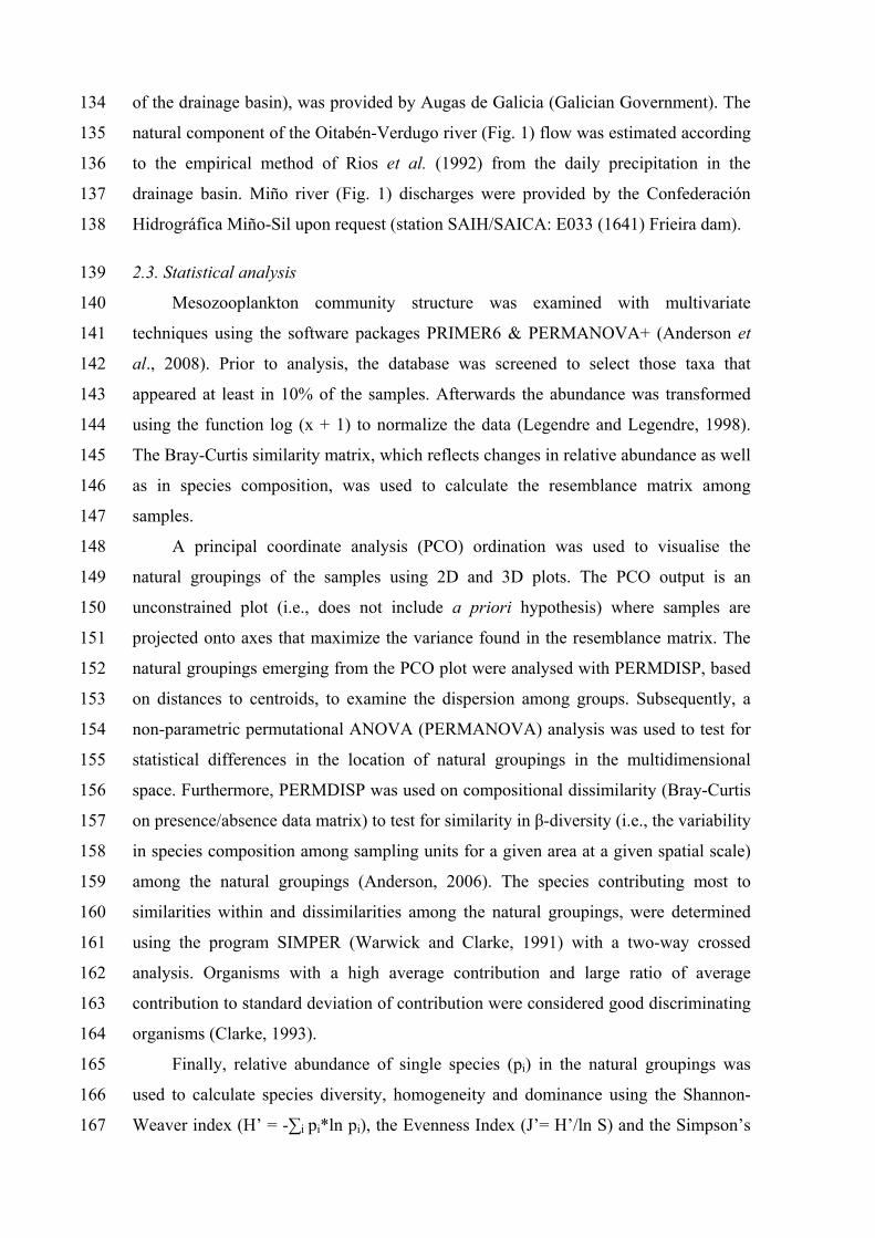
of the drainage basin), was provided by Augas de Galicia (Galician Government). The
natural component of the Oitabén-Verdugo river (Fig. 1) flow was estimated according
to the empirical method of Rios et al. (1992) from the daily precipitation in the
drainage basin. Miño river (Fig. 1) discharges were provided by the Confederación
Hidrográfica Miño-Sil upon request (station SAIH/SAICA: E033 (1641) Frieira dam).
134
135
136
137
138
139
140
141
142
143
144
145
146
147
148
149
150
151
152
153
154
155
156
157
158
159
160
161
162
163
164
165
166
167
2.3. Statistical analysis
Mesozooplankton community structure was examined with multivariate
techniques using the software packages PRIMER6 & PERMANOVA+ (Anderson et
al., 2008). Prior to analysis, the database was screened to select those taxa that
appeared at least in 10% of the samples. Afterwards the abundance was transformed
using the function log (x + 1) to normalize the data (Legendre and Legendre, 1998).
The Bray-Curtis similarity matrix, which reflects changes in relative abundance as well
as in species composition, was used to calculate the resemblance matrix among
samples.
A principal coordinate analysis (PCO) ordination was used to visualise the
natural groupings of the samples using 2D and 3D plots. The PCO output is an
unconstrained plot (i.e., does not include a priori hypothesis) where samples are
projected onto axes that maximize the variance found in the resemblance matrix. The
natural groupings emerging from the PCO plot were analysed with PERMDISP, based
on distances to centroids, to examine the dispersion among groups. Subsequently, a
non-parametric permutational ANOVA (PERMANOVA) analysis was used to test for
statistical differences in the location of natural groupings in the multidimensional
space. Furthermore, PERMDISP was used on compositional dissimilarity (Bray-Curtis
on presence/absence data matrix) to test for similarity in β-diversity (i.e., the variability
in species composition among sampling units for a given area at a given spatial scale)
among the natural groupings (Anderson, 2006). The species contributing most to
similarities within and dissimilarities among the natural groupings, were determined
using the program SIMPER (Warwick and Clarke, 1991) with a two-way crossed
analysis. Organisms with a high average contribution and large ratio of average
contribution to standard deviation of contribution were considered good discriminating
organisms (Clarke, 1993).
Finally, relative abundance of single species (pi) in the natural groupings was
used to calculate species diversity, homogeneity and dominance using the Shannon-
Weaver index (H’ = -∑i pi*ln pi), the Evenness Index (J’= H’/ln S) and the Simpson’s
index (λ = ∑ pi2), respectively (Omori an Ikeda, 1984). We calculated also the species
richness (S) of each natural grouping by counting the different taxa and the Margalef’s
index (d = (S-1)/log N), which is an index of the number of species for a given number
of individuals. The total abundance (N), as well as holoplankton and meroplankton
abundances (all expressed in individuals per 1000 m
168
169
170
171
172
173
174
175
176
177
178
179
180
181
182
183
184
185
186
187
188
189
190
191
192
193
194
195
196
197
198
199
200
201
-3) were calculated for each natural
grouping. Non-parametric analysis using Mann-Whitney U test (STATISTICA v6
software, StatSoft Inc., Tulsa, USA) was subsequently conducted to test if these biotic
variables varied significantly between natural groupings.
Three set of variables were considered to model the mesozooplankton community
structure: i) meteorologic variables: upwelling index (-Qx), fresh water inputs from the
rivers Oitabén-Verdugo (QrOi) and Miño (QrMi) and the moon, which was codified as
a categorical variable, dividing the lunar cycle into 4 periods following Hernández-
León et al. (2001); ii) hydrographic variables obtained from the CTD casts and Silleiro
and Rande observatories; and iii) biotic variables obtained from the natural groupings:
total abundance (N), holoplankton-meroplankton ratio (H/M), richness (S), diversity
(H’), homogeneity (J’), dominance (λ) and Margalef’s index (d). Prior to modelling, all
variables were tested for collinearity (Spearman correlation matrix) and those with
determination coefficients (R2) higher than 0.9 were omitted. The retained variables
were then transformed to compensate for skewness. Given that variables were
measured in different units, they were standardized prior to calculate the resemblance
matrix using Euclidean distance.
RELATE analysis was carried out to test if the spatial pattern of each set of
variables matched with the spatial pattern of the mesozooplankton samples, by
correlating the matching entries of the resemblance matrices based on the Spearman
rank correlation (ρ). Relationships between the resemblance matrix of
mesozooplankton and environmental-biotic variables were modelled with distance-
based linear models (DistLM). In order to assign the contribution of the different sets
of variables (meteorologic, hydrographic and biotic) to the total variability found in the
mesozooplankton resemblance matrix, a step-wise selection procedure was carried out
using the adjusted R2 as selection criterion. The output of the fitted model in multi-
dimensional space was visualized with distance-based redundancy analysis (dbRDA)
(McArdle and Anderson, 2001).
Finally, all significant variables were introduced in the model with the “best”
procedure of the DistLM model, using the bayesian information criterion (BIC),
because it includes a more severe penalty for the inclusion of new predictor variables
than Akaike’s information criterion (AIC). Such a procedure allowed us to generate the
simplest model that explained the highest variability found in the mesozooplankton
resemblance matrix. Finally, the output of the fitted model in multi-dimensional space
was visualized with distance-based redundancy analysis (dbRDA).
202
203
204
205
206
207
208
209
210
211
212
213
214
215
216
217
218
219
220
221
222
223
224
225
226
227
228
229
230
231
232
233
234
3. Results
3.1. Hydrography and dynamics
The main forcing variables affecting the hydrography of the Ría de Vigo and
adjacent shelf are presented in Fig. 2 and the CTD profiles of innermost transect 2 (T2)
and outermost transect 5 (T5) shown in Fig. 3. Surveys 1 to 4 (from July 2 to 11) were
conducted under wind relaxation/downwelling conditions, characterised by weak
winds of variable direction and a monotonic increase of SST (Fig. 2a, b, d), with the
exception of the strong downwelling-favourable winds recorded on July 4 (Fig. 2a, b)
resulting in a strong northward current (Fig. 2c). The downwelling/relaxation event
gradually warmed the surface layer, increasing the stratification (Fig. 3a, b), leading to
the deepening of the Chl-a maximum and posterior dispersion through the water
column (Fig. 3c).
Surveys 5 to 10, conducted from September 26 to October 14, were characterised
by upwelling-favourable winds (Fig. 2a, b) that cooled the surface layer sharply (Fig.
2d). The dynamics were more complex during these surveys with four well-defined
periods: i) from September 25 to 28 weak winds of variable direction prevailed,
accompanied by surface layer warming and stratification (Figs. 2a, d, 3a, b); ii) from
September 29 to October 4 upwelling-favourable winds resulted in strong south-
westward currents and a sharp cooling of the water column, that uplifted the Chl-a
maximum close to the surface, with Chl-a levels being twice as much in T2 than in T5
(Fig. 2a, c, 3c); iii) from October 5 to 8 sustained south-southwestward winds reversed
the circulation pattern and warm oceanic surface water was advected to the coast
increasing the stratification (Figs. 2a, c, d, 3a); and iv) from October 9 to 13, north-
eastward winds favoured coastal upwelling resulting in strong westward currents,
water column cooling and Chl-a maximum export to the ocean (Figs. 2a, c, d, 3a, c).
The last survey (October 14) was dominated by weak winds of variable direction and a
reversal of the circulation pattern that warmed the water increasing the stratification
and lowering Chl-a (Figs. 2a, c, d, 3a, c).
In summary, whilst surveys 1 to 4 (July) occurred under predominantly summer-
downwelling conditions with similar Chl-a levels inside and outside the Ría de Vigo,
autumn-upwelling conditions prevailed during surveys 5 to 10 (September - October)
with higher Chl-a levels in the coastal (T2) than in the mid-shelf (T5) domains.
Autotrophy prevailed in the upper 10 m throughout the surveys, except on July 11 and
October 3, when heterotrophy was dominant (Fig. 3d).
235
236
237
238
239
240
241
242
243
244
245
246
247
248
249
250
251
252
253
254
255
256
257
258
259
260
261
262
263
264
265
266
267
268
3.2. Mesozooplankton communities
It should be noted that the net used in this study could bias the mesozooplankton
size range (0.2 - 20 mm) towards relatively large-size animals. However, the high
abundance of phytoplankton in the samples clogged the net avoiding this bias, thus
capturing animals of less than 375 µm as harpacticoid copepods or foraminifera.
The PCO plot (Fig. 4) shows three well-defined groups across the PCO1 axis,
which accounted for 47.3% of the variability of the resemblance matrix. The samples
at the extremes of that axis corresponded to T5 and T2 respectively, with T5 having
negative values and oceanic fauna (as hyperiids or adults of euphausiids), while T2 had
positive values and larval stages of coastal species. Samples in between the oceanic
and coastal domains (between –25 and +5 in the PCO1 axis) grouped together with a
large dispersion and were considered collectively as frontal samples. Therefore, the
PCO1 axis reflected the gradient from oceanic to coastal stations, with transition
frontal stations among them.
The PCO2 axis explained 14.2 % of the variability of the resemblance matrix and
it was strongly related with the two sampling periods: summer-downwelling (positive
values of PCO2) and autumn-upwelling (negative values of PCO2). Within the
summer-downwelling frontal group there were three outliers (PCO2 values around
+40) that corresponded to samples with high abundances of calyptopis stages (1260-
3090 ind m-3).
Based on the PCO plot (Fig. 4) and the previous analysis of the hydrography and
dynamics of the study area, samples were grouped according to two factors (sampling
period/hydrographic characteristics and coast-ocean gradient) into 6 communities:
summer-downwelling coastal (SC), summer-downwelling frontal (SF), summer-
downwelling oceanic (SO), autumn-upwelling coastal (AC), autumn-upwelling frontal
(AF) and autumn-upwelling oceanic (AO).
The test for dispersions among communities with PERMDISP revealed statistical
differences in summer between SF-SC (p < 0.05) and in autumn between AF-AO and
AC-AO (p < 0.05). PERMANOVA tests revealed that all the communities were
statistically different in a multidimensional space (Table 1). However, such a
difference can be in species composition and/or abundance. Variability in species
composition (β-diversity) revealed that in summer-downwelling conditions, the coastal
community differed significantly (p < 0.001) from the oceanic and frontal
communities, which were similar in composition between them. Autumn-upwelling
communities displayed also compositional differences between coastal and frontal-
oceanic communities, but marginally significant (p = 0.07). Besides, coastal
communities varied in composition between sampling periods (p = 0.001), but the
frontal and oceanic communities did not. PERMANOVA tests revealed no significant
differences (p = 0.375) between the surface and oblique hauls. However, samples were
not merged together because certain species did vary between the two strata. In fact, in
some cases the surface and column samples obtained in the same transect belonged to
different communities (Fig. 5, day 4).
269
270
271
272
273
274
275
276
277
278
279
280
281
282
283
284
285
286
287
288
289
290
291
292
293
294
295
296
297
298
299
300
301
302
Average abundances of the taxa that contributed most to the within-group
similarity, i.e. the discriminating species, appear in Table 2 as well as the different taxa
within each community that are summarised in Annexe 1. In summer, coastal waters
were dominated by copepods (24 species), larval stages of the euphausiid Nyctiphanes
couchii, echinoderm larvae and appendicularians. Frontal waters were dominated by
larval stages of the euphausiid N. couchii, copepods (17 species), and salps. In contrast,
oceanic waters were dominated by salps, copepods (18 species) and euphausiids (13%
adults). In autumn, coastal waters differed markedly from summer with echinoderm
larvae, larval stages of N. couchii, appendicularians, copepods (25 species), cirripeds
and decapods contributing the most. Frontal waters were dominated by larval stages of
N. couchii, copepods (20 species), salps and chaetognaths. Finally, oceanic waters
were dominated by salps, copepods (18 species), euphausiids (49% adults) and
chaetognaths (Fig. 6).
The species that contributed most to discriminate between pairs of communities
are presented in Table 3. Spatial dissimilarities among communities were consistent
through summer and autumn, with the highest dissimilarity between coastal and
oceanic samples (the most distant communities), then coastal and frontal samples and,
finally, the lower dissimilarity was found between frontal and oceanic communities.
Discriminating species present in the upper part of Table 3 are good indicators of
changes in space due to water body preferences (meroplankton present in the coastal
domain versus holoplankton present in the oceanic domain). In contrast, temporal
dissimilarities among communities showed that coastal and oceanic communities
changed less with time (38.78 and 37.71%, respectively) than the frontal community
(45.96%). Discriminating species between both sampling periods give an idea of the
zooplankton succession due to different life cycle strategies and/ or due to the different
upwelling/downwelling situations.
303
304
305
306
307
308
309
310
311
312
313
314
315
316
317
318
319
320
321
322
323
324
325
326
327
328
329
330
331
332
333
334
335
It is noticeable the contrasting levels of similarity found for the holoplankton and
meroplankton components within each community (Table 4). While the holoplankton
was quite similar across the communities, with the frontal community showing the
lowest values; the meroplankton was more variable showing a decreasing gradient of
similarity from coastal to oceanic communities. Comparisons between communities
revealed that the holoplankton component changed less spatially and temporally than
the meroplankton. The later showed enormous differences between coastal and oceanic
samples, as well as a marked change in the frontal and oceanic communities of both
sampling periods.
The biotic indices obtained from the different communities are presented in Table
5 and their spatial and temporal non-parametric comparisons are summarized in Table
6. In summer, there was a marked gradient between the coastal and the frontal-oceanic
domains: the coastal community had the highest diversity and abundance, with many
species almost homogenously distributed and the lowest ratio between holoplankton
and meroplankton, due to the high abundance of larval stages of coastal species (Table
5, Fig. 6). The frontal community was very similar to the oceanic one but with
significant differences in richness and abundance (3-fold in the frontal than in the
oceanic samples). In the oceanic community, there was a remarkable decline of
meroplankton, with almost all the animals present in the oceanic sample being
holoplankton. In autumn, there were less significant differences between coastal and
frontal-oceanic communities, except in total abundance and richness that followed the
previously described coastal-frontal-oceanic gradient (Fig. 6, Table 6).
Coastal waters underwent larger changes between sampling periods, with less
richness, diversity and, consequently, lower evenness and higher dominance in autumn
than in summer. However, there was no statistical difference between meroplankton
and holoplankton although there was more meroplankton in the autumn coastal
community (Fig. 6). The structure of frontal and oceanic communities did not vary
much between both periods, except for a marked decrease in autumn abundance for
both communities, mainly due to a decrease in holoplankton.
336
337
338
339
340
341
342
343
344
345
346
347
348
349
350
351
352
353
354
355
356
357
358
359
360
361
362
363
364
365
366
367
368
369
The significant relationships of the correlations between CTD variables and the
discriminating taxa are summarized in Table 7. Species more abundant in coastal
waters (i.e. Pisidia longicornis zoea, echinoderm zoea, cirripedia zoea, processidae
zoea, appendicularians) showed negative correlations with Salt and positive
correlations with Stab, common features of coastal areas influenced by continental
runoff. Frontal communities (i.e. brachyura megalopa, Calanus helgolandicus,
Calanoides carinatus, Acartia clausi) correlated negatively with AOU, related with
higher phytoplankton activity. Conversely, oceanic communities (i.e. salps, mysidacea,
Paraeuchaeta hebes, hyperiids) correlated positively with Tº and Salt and negatively
with Chl-a and Stab.
3.3. Linking environmental and biotic variables with mesozooplankton communities
The ordination scores of the PCO 1 and 2 axes on each station were regressed
against the meteorologic, hydrographic and dynamic variables obtained from the
Silleiro and Rande observatories to determine the relative importance of each forcing
factor and the delay of the response of the community structure. All variables showed
better correlations with the scores of the PCO2 axis and the delay intervals varied
depending on the variable (Table 8). These correlation coefficients were used to weight
the effect of the forcing variables recorded at the Silleiro and Rande observatories on
each sampling station. Eighteen variables were retained based on collinearity analysis.
The variables Chl-a, Stab, N and H/M were log transformed to compensate for
skewness.
The retained variables were then run with the “best” procedure of the DistLM
model, using the Bayesian information criterion (BIC). As a result, only five variables
were retained by the model, together accounting for 64% of the variability found in the
mesozooplankton resemblance matrix (Table 9, Fig. 7). Three of the five fitted
variables were biotic: log (H/M), log (N) and S, the fourth was –Qx and the fifth was
the moon. The first two dbRDA axes accounted with 88.3% of the fitted variability,
corresponding to 55.4% of the total variability of the resemblance matrix. This model
based only on five variables clearly represented the community patterns shown in the
unconstrained PCO plot of Fig. 4 (RELATE analysis ρ = 0.58, p < 0.001),
demonstrating that the main structuring forces of the data cloud were included in the
model. Thus, attending to the variable vectors overlaid in Fig. 7 it can be concluded
that the most important variables involved in originating the coastal–oceanic gradient,
were log (H/M) inversely and log (N) together with S directly (also shown in Table 5).
Such a gradient was a consequence of very rich, abundant and meroplankton-
dominated coastal waters facing poor, less abundant and holoplankton-dominated
oceanic waters. On the other hand, the sampling period/hydrographic characteristics
found in the Y axis were directly related with the moon and log (N) and negatively
with -Qx, because summer waters were dominated by high-abundance downwelled
waters while autumn waters were dominated by low-abundance upwelled waters with
higher contribution of meroplankton. The last quarter of the moon (waning crescent)
was directly related with increased abundances of mesozooplankton in summer, while
the first three quarters where correlated with autumn waters. The first and third
quarters (waxing crescent and waning gibbous) were correlated with high abundance
autumn coastal communities and the second quarter (waxing gibbous) was correlated
with autumn frontal and oceanic communities, where less abundance was found.
370
371
372
373
374
375
376
377
378
379
380
381
382
383
384
385
386
387
388
389
390
391
392
393
394
395
396
397
398
399
400
401
402
403
RELATE analysis showed that the spatial patterns based on the meteorologic (ρ =
0.174, p < 0.01), hydrographic (ρ = 0.285, p < 0.01), and biotic data (ρ = 0.67, p <
0.001) were significantly related to the patterns found in the mesozooplankton
resemblance matrix, with the optimal match (largest Spearman ρ) corresponding to
biotic data. The output of marginal tests on each set of variables showed that biotic
data accounted for 54.5%, hydrography for 48.8% and meteorology for 39.9% of the
variability (Table 10). However, when fitted into the step-wise model grouping the
variables according to the three sets of variables, the DistLM model revealed that the
variability found in the mesozooplankton resemblance matrix was better described by
the biotic variables (54.5%), followed by the hydrography (16.1%) and finally the
meteorology (6.0%); altogether accounting 76.6% of the total variability found in the
mesozooplankton resemblance matrix (Fig. 8).
The same analyses were performed splitting the mesozooplankton data matrix in
holoplankton and meroplankton components to filter out the main descriptor of the
community. PCO analysis revealed that while the holoplankton shared almost the same
structuring forces as found for the mesozooplankton (41.7% corresponding to the
coast-ocean gradient and 18.1% corresponding to sampling period/hydrographic
characteristics, ρ = 0.956, p < 0.001), the meroplankton did it to a lesser extent (only
30.6% corresponding to the coast-ocean gradient and 11.9 % to the sampling
period/hydrographic characteristics, ρ = 0.703, p < 0.001). Furthermore, the spatial
patterns based on the resemblance matrix of the explicative variables (meteorologic,
hydrographic, and biotic without log (H/M)), were significantly better represented by
the resemblance matrix of holoplankton (ρ = 0.454, p < 0.001) than that of the
meroplankton (ρ = 0.261, p < 0.01). DistLM model run with the “step-wise” procedure
and BIC as selection criterion revealed that while the variability found in the
holoplankton resemblance matrix was better described by five variables (log (N)
28.2%, d 12.3%, -Qx 10.4%, moon 4 4.9% and Salt 2.8%, altogether accounting with
58.6%) the meroplankton was better described by three variables (S 19%, log (N) 9.2%
and –Qx 4.5% altogether accounting with 32.7%).
404
405
406
407
408
409
410
411
412
413
414
415
416
417
418
419
420
421
422
423
424
425
426
427
428
429
430
431
432
433
434
435
436
437
4. Discussion
4.1. Mesozooplankton communities
Mesozooplankton communities have been characterised at the short-time (< 1
wk) and spatial (< 11 km) scale for the first time in the Ría de Vigo. A total of six
mesozooplankton communities were identified according to their species composition
and abundance, together with the influence of the meteorology and hydrography of the
Ría de Vigo and adjacent shelf. As a consequence of the circulation pattern during
upwelling/downwelling events (Souto et al., 2003), part of the biomass produced
inside (outside) the Ría de Vigo is transported offshore (onshore) by the surface ocean
ward (coastal ward) current (Álvarez-Salgado et al., 2002, Spyrakos et al., 2011).
Therefore, the communities present in the Ría de Vigo might be disrupted and mixed
by this highly advective coastal upwelling/downwelling environment (González et al.,
2005). Indeed, such an effect can be tracked in our samples. Following the time-course
of the mesozooplankton community found at T3, it is clear how it changed in parallel
with the meteorology: On July 9, the mesozooplankton collected in surface waters
(Fig. 5a, number 3) belonged to the coastal community. On July 10, southerly winds
transported surface warm oceanic waters onshore (Figs. 2a, c, d, 3a), thus changing the
surface sample collected on July 11 to an oceanic community (Fig. 5a). At the same
time, the water column sample of July 11 (Fig. 5b) belonged to the frontal community,
due to the diminishing effect of the wind stress with depth. So, there were two different
communities in the same transect at different depths, although the methodology used in
this study (bongo sampling) was not the optimal to explore such differences.
The large dispersion found in frontal communities (Fig. 4) is a consequence of
their location between the coastal and oceanic domains and the continuous intrusions
of animals from both communities forced by the upwelling/downwelling currents.
Nonetheless, such intrusions did not lead to a continuous gradient between coastal and
oceanic realms caused by the mixing of the three communities. Intriguingly, the
persistence of the three communities suggests specific mesozooplankton responses,
like behavioural distribution patterns coupled with the residual circulation of the Ría de
Vigo (Marta-Almeida et al., 2006; Queiroga et al., 2007), that would allow the return
of advected animals to their community of origin.
438
439
440
441
442
443
444
445
446
447
448
449
450
451
452
453
454
455
456
457
458
459
460
461
462
463
464
465
466
467
468
469
470
471
4.2. Coastal-oceanic gradient
The natural groupings represented in the PCO plot (Fig. 4) clearly differentiate
coastal from frontal and oceanic waters. The latter were not different in species
composition but in abundance (more than 3-fold in the frontal than in the oceanic
samples) in both seasons (Table 5). Coastal waters differed from oceanic waters,
because neritic holoplankton species such as Temora longicornis, Acartia clausi,
Pseudocalanus elongatus, Paracalanus parvus (Peterson, 1998; Gaard, 1999) coexist
with meroplankton near the coast, therefore increasing notably the abundance of
coastal communities (Fusté and Gili, 1991; Bode et al., 1998, 2009; Blanco-Bercial et
al., 2006). Indeed, the largest mesozooplankton abundance occurred in the coastal
domain, both in summer and autumn, with meroplankton contributing 31.7 and 47.2%,
respectively. Coastal waters act as nursery areas in the Ría de Vigo, as found in long-
term studies off Galicia (Bode et al., 2009). The meroplankton contribution clearly
declined in the frontal (2.3 and 3.6% on each sampling period) and even more in the
oceanic community (only 0.6 and 0.4%). Furthermore, a decreasing similarity from
coastal to oceanic communities (Table 4) was coupled with this decline in
meroplankton abundance. Therefore, it can be concluded that the coastal-oceanic
gradient was mainly due to a gradient in holoplankton/meroplankton abundance, as
shown in Fig. 7 and reinforced by the high contribution of this ratio (39.6%) describing
the overall variability found in the mesozooplankton resemblance matrix (Table 9).
The ratio (H/M) is proposed as an index for mesozooplankton community studies
in coastal and shelf areas. Indeed, there is a need for a consensus between the
taxonomists involved with data acquisition to avoid the difficulties inherent when
comparing zooplankton time series (Perry et al., 2004; Valdés et al., 2007). The
adoption of the ratio (H/M) as a consensus index is supported by the following
advantages: i) the easiness of obtaining the data due to its independency on the degree
of taxonomic expertise (the recognition of meroplankton and holoplankton groups is an
easy task, even with plankton-imaging software as in Benavides et al. (2010)); ii) its
high power describing the variability found in mesozooplankton communities (39.6%
against 9.7% explained by Shannon’s diversity index, H’, which deeply depends on the
taxonomic expertise); iii) less time and effort for obtaining data; iv) its independency
on the biomass given that is a ratio of individuals. Furthermore, the ratio (H/M) may be
used to place other people’s works into mesozooplankton coastal-oceanic community
gradients, as well as to track mesozooplankton communities advected by mesoscale
oceanographic events like filaments, gyres, upwelling/downwelling (Relvas et al.,
2007).
472
473
474
475
476
477
478
479
480
481
482
483
484
485
486
487
488
489
490
491
492
493
494
495
496
497
498
499
500
501
502
503
504
505
4.3. Short-term changes in mesozooplankton communities
There was a noticeable change between summer and autumn communities,
originated by contrasting oceanographic conditions coupled with zooplankton life
strategies. Summer surveys were carried out under downwelling-relaxation conditions.
The predominant southerly winds pushed onshore warm and salty surface waters of
subtropical origin (Souto et al., 2003; Spyrakos et al., 2011), carrying oceanic species
positively correlated with Salt and Tº and negatively correlated with Chl-a (salps,
mysids, hyperiids, Paraeuchaeta hebes), as found in other works (Valdés et al., 1990;
Blanco-Bercial et al., 2006). These subtropical waters had less richness and abundance
than coastal waters, with the salps Salpa fusiformis and Thalia democratica dominating
the samples (Huskin et al., 2003; Boero et al., 2008). The frontal community was
similar in composition to the oceanic, but differed in abundance due to the onshore
advection that piled up oceanic species in the front, with N. couchii larval stages
dominating the samples (Fig. 6). Discriminating taxa found in frontal waters were
negatively correlated with AOU (brachyuran megalopae, Calanus helgolandicus,
Calanoides carinatus, A. clausi), suggesting that these animals were present in waters
with high primary production as found by Blanco-Bercial et al. (2006). Coastal waters
were dominated by species positively correlated with Stab and Chl-a and negatively
correlated with Salt as appendicularians (Acuña and Anadón, 1992), meroplankton
(cirriped, echinoderm, crustacean, polychaete and gastropod larvae), and cladocerans,
which are species specialized to feed on small particles (Blanco-Bercial et al., 2006).
The copepod A. clausi was exceptionally abundant in coastal waters far followed by T.
longicornis (Bode et al., 2009).
Autumn surveys occurred under dominant upwelling conditions, which resulted
in less difference between coastal and frontal communities, because coastal waters
were advected offshore against the frontal community. Species found in the coastal
community correlated positively with AOU, Stab (meroplankton, siphonophores and
appendicularians) and Chl-a (Oithona plumifera). This community showed marked
changes in their composition compared with summer, with increased numbers of
siphonophores, chaetognaths, echinoderm larvae and O. plumifera, which is an
upwelling indicative species (Blanco-Bercial et al., 2006); and decreased numbers of
cladocerans (Podon intermedius and Evadne nordmanni) and the copepods A. clausi,
T. longicornis, Centropages chiercheai and Clausocalanus spp. The frontal community
was characterised by animals negatively correlated with AOU and positively correlated
with Chl-a and Stab as chaetognaths, siphonophores, N. couchii larvae, gastropods, and
the copepods C. carinatus, C. helgolandicus, P. parvus and A. clausi, that are
considered coastal upwelling species (Peterson, 1998). Increased abundances of
chaetognaths, mysidaceans, P. parvus and Paraeuchaeta spp. were found in autumn
frontal communities; while decreased numbers of brachyuran zoea and megalopa,
gastropods, furcilia stages of N. couchii and the copepods P. hebes, C. helgolandicus
and C. carinatus were found in autumn compared with summer. Finally, oceanic
waters showed an increase in autumn abundances of N. couchii adults and larval
stages, chaetognaths, mysidaceans and P. parvus; while a marked decrease in salps, P.
hebes, P. spp., C. carinatus and C. helgolandicus was noted compared to the summer
oceanic community. These seasonal changes are in agreement with previous works
(Valdés et al., 1990; Bode et al., 1998, 2004; Blanco-Bercial et al., 2006; Huskin et al.
2006).
506
507
508
509
510
511
512
513
514
515
516
517
518
519
520
521
522
523
524
525
526
527
528
529
530
531
532
533
534
535
536
537
538
539
Huge numbers of N. couchii calyptopis (ranging from 282-3090 ind m-3) found in
the frontal community of July 2 (transects 3 and 4) coincided with the highest
aggregation of adults (170 ind m-3, dominated by mature females carrying fully
developed eggs) at the outer transect number 5. Furthermore, N. couchii adult
aggregations were found again in autumn frontal communities on October 9 and 10
(139 and 123 ind m-3 respectively), coinciding with calyptopis abundances ranging
from 540-2395 ind m-3. This spatial distribution of larvae mainly in the coastal and
frontal domains coupled with the high abundance of mature adults in the frontal and
oceanic domains, suggest a breeding aggregation of adults through the upwelling
season, which coincides with the reproductive ecology of this species (Mauchline,
1984).
The oceanographic situation found in this study, i.e. downwelling in summer and
upwelling in autumn, was opposite to the main oceanographic pattern off NW Spain,
where coastal winds describe a seasonal cycle, favour upwelling from March-April to
September-October and downwelling for the rest of the year (Wooster et al., 1976;
Blanton et al., 1987). However, more than 70% of the wind variability concentrates on
periods of 10-20 days, thus allowing the frequent occurrence of downwelling events
during the upwelling season (Álvarez-Salgado et al., 2002). Therefore, the
downwelling event experienced during summer samplings may account for the
unexpected massive amounts of salps found in the oceanic community (maximum of
995 salps m
540
541
542
543
544
545
546
547
548
549
550
551
552
553
554
555
556
557
558
559
560
561
562
563
564
565
566
567
568
569
570
571
572
573
-3), although their natural cycle place these animals at the end of the
upwelling season, occurring along the offshore edge of the shelf break salinity fronts
(Huskin et al., 2003; Blanco-Bercial et al., 2006; Huskin et al., 2006; Deibel and
Paffenhöfer, 2009) when high salinity water flows poleward along the Portuguese and
Galician coasts (Haynes and Barton, 1990; Castro et al., 1997). Furthermore, the
presence of the warm-water copepod Temora stylifera (Villate et al., 1997; Valdés et
al., 2007; Bode et al., 2009) in summer oceanic waters reinforces the unusual
oceanographic conditions experienced during July samplings. Hence, we would like to
point out that the mesozooplankton community composition found in summer
samplings may be distorted by the unusual oceanographic conditions and the
abundance of salps (Huskin et al., 2003).
4.4. Linking mesozooplankton communities to environment: to what extent?
The relationship between environment and plankton is difficult to generalise,
because the environmental factors interact at different temporal scales (Bode et al.
2009; Nogueira et al. 2011) aside from indirect interactions canalized through the food
web that gradually diminish along the trophic levels resulting in a weakening effect
(Micheli, 1999). In this work, only two days were enough to change the community
present in the surface sample of T3 from coastal to oceanic (Fig. 5a, day 4). Such a
quick change contrast with the delay of weeks found between the time series and the
zooplankton response by Tenore et al. (1995), or the lack of apparent response of
plankton to climate forcing found at mid latitudes compared to boreal locations
(Beaugrand et al., 2000). Although, coastal communities shifted to oceanic due to
wind-driven currents produced the same day and the day before, the coastal-ocean
gradient was better explained by the biotic variables (log (H/M), 39.6%) than those
directly related with surface currents (u and v, altogether explaining 10.8%) or
indirectly related (-Qx, 8.3%). This large difference between the explanatory power of
biotic and environmental variables may play some part in the delays obtained by other
authors (Tenore et al., 1995; Bode et al. 2009; Nogueira et al., 2011) or even the lack
of response (Beaugrand et al., 2000).
574
575
576
577
578
579
580
581
582
583
584
585
586
587
588
589
590
591
592
593
594
595
596
597
598
599
600
601
602
603
604
605
606
607
Another complication that may mask the link between environment and plankton
is that the environmental conditions are more tightly linked with the holoplankton than
with the meroplankton. This difference may be produced by the low abundance and the
high variability found in the meroplankton samples of the frontal and oceanic
communities (Table 4). However, the contrasting life-history characteristics of both
planktonic components may play some part in their link with the environment given
that the holoplankton spends their entire life in the pelagic realm, and the
meroplankton spends but a part of their life in the water column.
An interesting finding was the significant contribution of the moon describing the
mesozooplankton variability. Although there are few samplings to reveal how the
moon is influencing the zooplankton abundance, we find that the different moon
periods affect unequally the holoplankton and meroplankton components. We ignore
whether the zooplankton reproductive strategies are coupled with specific moon
periods by means of its light intensity and/or with the tidal currents (Tankersley et al.,
2002; Queiroga et al., 2007) and requires further study. However, we discard the moon
effect through the predatory influence of diel vertical migrators (Hernández-León et
al., 2001), because such predators are not present in the study area but in pelagic open
ocean environments.
5. Conclusions
Three well-defined mesozooplankton communities named as coastal, frontal and
oceanic were defined by means of their abundance and specific composition in the Ría
de Vigo. These communities changed from summer to autumn due to a shift in coastal
upwelling/downwelling conditions coupled with taxa dependent changes in life cycle
strategies. The main factor responsible of the coastal-oceanic gradient was the ratio
between holoplankton and meroplankton, which was increasing from coastal to the
oceanic community. This ratio has been proposed as a consensus index for coastal-
shelf zooplankton community studies due to its explicative power and easiness of
identification. The episodic upwelling/downwelling events off the Ría de Vigo create
an advective environment where zooplankton faces forcible removal from the
ecosystem. However, the communities kept their integrity throughout the upwelling
season in spite of being displaced by the offshore/onshore currents, presumably due to
behavioural changes in their vertical position. This study brings light into the
traditionally overlooked mesozooplankton fraction of the Ría de Vigo, an essential
component of the pelagic realm that channels the high productivity of the Ría de Vigo
up to higher trophic levels.
608
609
610
611
612
613
614
615
616
617
618
619
620
621
622
623
624
625
626
627
628
629
630
631
632
633
634
635
636
637
638
639
Acknowledgements
We are indebted to the captain, crew and technicians of R/V “Mytilus” (IIM,
CSIC Vigo), for their assistance in collecting the zooplankton samples and
hydrographic data. We acknowledge the enormous patience of Félix Álvarez, which
sorted by hand every single salp out of the samples, as well as Mariana Rivas. We
would like to thank Silvia Piedracoba, Francisco de la Granda and to Puertos del
Estado, MeteoGalicia, Augas de Galicia and the Confederación Hidrográfica Miño-Sil
for providing the meteorological and hydrographic data. The authors thank the three
anonymous reviewers for their effort, which improved the quality and clarity of the
manuscript. This study was supported by the projects CAIBEX (Spanish Ministry of
Innovation and Science CTM2007-66408-C02) and LARECO (CTM2011-25929),
FEDER Funds and the first author by a JAE-pre grant (CSIC) cofinanced with Fondo
Social Europeo (ESF) funds.
References
Acuña, J.L., Anadón, R., 1992. Appendicularian assemblages in a shelf area and their
relationship with temperature. Journal of Plankton Research 14 (9), 1233-1250.
Álvarez-Salgado, X.A., Beloso, S., Joint, I., Nogueira, E., Chou, L., Pérez, F.F.,
Groom, S., Cabanas, J.M., Rees, A.P., Elskens, M., 2002. New production of the
NW Iberian shelf during the upwelling season over the period 1982-1999. Deep
Sea Research Part I: Oceanographic Research Papers 49 (10), 1725-1739.
Anderson, M.J., 2006. Distance-based tests for homogeneity of multivariate
dispersions. Biometrics 62, 245-253.
Anderson, M.J., Gorley, R.N., Clarke, K.R., 2008. PERMANOVA+ for PRIMER:
Guide to software and statistical methods. PRIMER-E, Plymouth, UK.
Arístegui, J., Álvarez-Salgado, X.A., Barton, E.D., Figueiras, F.G., Hernández-León,
S., Roy, C., Santos, A.M.P., 2006. Oceanography and Fisheries of the Canary
Current/Iberian Region of the Eastern North Atlantic. In: A.R. Robinson and Brink,
K.H. (Eds.), The Sea. The Global Coastal Ocean: Interdisciplinary Regional
Studies and Syntheses. Harvard University Press, Cambridge, UK, pp. 877-931.
Bakun, A., 1973. Coastal upwelling indices, west coast of North America, 1946-71.
NOAA Technical Report NMFS SSRF 671. Seatle, US Dept. Commerce.
640
641
642
643
644
645
646
647
648
649
650
651
652
653
654
655
656
657
658
659
660
661
662
663
664
665
666
667
668
669
670
671
672
673
Batten, S.D., Fileman, E.S., Halvorsen, E., 2001. The contribution of
microzooplankton to the diet of mesozooplankton in an upwelling filament off the
north west coast of Spain. Progress In Oceanography 51 (2-4), 385-398.
Beaugrand, G., Ibañez, F., Reid, P.C., 2000. Spatial, seasonal and long-term
fluctuations of plankton in relation to hydroclimatic features in the English
channel, Celtic Sea and Bay of Biscay. Marine Ecology Progress Series 200, 93-
102.
Benavides, M., Echevarría, F., Sánchez-García, R., Garzón, N., González-Gordillo,
J.I., 2010. Mesozooplankton community structure during summer months in the
Bay of Cádiz. Thalassas 26 (2), 103-118.
Blanco-Bercial, L., Álvarez-Marqués, F., Cabal, J.A., 2006. Changes in the
mesozooplankton community associated with the hydrography off the northwestern
Iberian Peninsula. ICES Journal of Marine Science 63 (5), 799-810.
Blanton, J.O., Tenore, K.R., Castillejo, F., Atkinson, L.P., Schwing, F.B., Lavin, A.,
1987. The relationship of upwelling to mussel production in the rias on the western
coast of Spain. Journal of Marine Research 45 (2), 497-511.
Bode, A., Álvarez-Ossorio, M.T., González, N., 1998. Estimations of
mesozooplankton biomass in a coastal upwelling area off NW Spain. Journal of
Plankton Research 20(5), 1005-1014.
Bode, A., Alvarez-Ossorio, M.T., Barquero, S., Lorenzo, J., Louro, A., Varela, M.,
2003a. Seasonal variations in upwelling and in the grazing impact of copepods on
phytoplankton off A Coruña (Galicia, NW Spain). Journal of Experimental Marine
Biology and Ecology 297, 85–105.
Bode, A., Carrera, P., Lens, S., 2003b. The pelagic foodweb in the upwelling
ecosystem of Galicia (NW Spain) during spring: natural abundance of stable
carbon and nitrogen isotopes. ICES Journal of Marine Science 60 (1), 11-22.
Bode, A., Alvarez-Ossorio, M.T., Carrera, P.L., Lorenzo, J., 2004. Reconstruction of
trophic pathways between plankton and the North Iberian sardine (Sardina
pilchardus) using stable isotopes. Scientia Marina 68 (1), 165-178.
Bode, A., Alvarez-Ossorio, M.T., Cabanas, J.M., Miranda, A., Varela, M., 2009.
Recent trends in plankton and upwelling intensity off Galicia (NW Spain). Progress
In Oceanography 83 (1-4), 342-350.
Boero, F., Bouillon, J., Gravili, C., Miglietta, M.P., Parsons, T., Piraino, S., 2008.
Gelatinous plankton: irregularities rule the world (sometimes). Marine Ecology
Progress Series 356, 299-310.
674
675
676
677
678
679
680
681
682
683
684
685
686
687
688
689
690
691
692
693
694
695
696
697
698
699
700
701
702
703
704
705
Calvet, A., Saiz, E., 2005. The ciliate-copepod link in marine ecosystems. Aquatic
Microbial Ecology 38(2), 157-167.
Castro, C.G., Álvarez-Salgado, X.A., Figueiras, F.G., Fraga Rodríguez, F., Pérez, F.F.,
1997. Transient hydrographic and chemical conditions affecting microplankton
populations in the coastal transition zone of the Iberian upwelling system (NW
Spain) in September 1986. Journal of Marine Research 55, 321-352.
Cermeño, P., Marañón, E., Pérez, V., Serret, P., Fernández, E., Castro, C.G., 2006.
Phytoplankton size structure and primary production in a highly dynamic coastal
ecosystem (Ría de Vigo, NW-Spain): Seasonal and short time scale variability.
Estuarine Coastal and Shelf Science 67, 251-266.
Clarke, K.R., 1993. Non-parametric multivariate analyses of changes in community
structure. Austral Ecology 18 (1), 117-143.
Clarke, K.R., Ainsworth, M., 1993. A method of linking multivariate community
structure to environmental variables. Marine Ecology Progress Series 92, 205-219.
Clarke, K.R., Green, R.H., 1988. Statistical design and analysis for a "biological
effects" study. Marine Ecology Progress Series 46 (1-3), 213-226.
Crespo, B.G., Figueiras, F.G., Porras, P., Teixeira, I.G., 2006. Downwelling and
dominance of autochthonous dinoflagellates in the NW Iberian margin: the
example of the Ría de Vigo. Harmful Algae 5, 770-781.
Deibel, D., Paffenhöfer, G.A., 2009. Predictability of patches of neritic salps and
doliolids (Tunicata, Thaliacea). Journal of Plankton Research 31 (12), 1571-1579.
Ferreiro, M.J., Labarta, U., 1988. Distribution and abundance of sardine eggs in the Ria
of Vigo (NW Spain), 1979–1984. Journal of Plankton Research 10 (3), 403-412.
Fusté, X., Gili, J.M., 1991. Distribution pattern of decapod larvae off the north-western
Iberian Peninsula coast (NE Atlantic). Journal of Plankton Research 13 (1), 217-
228.
Gaard, E., 1999. The zooplankton community structure in relation to its biological and
physical environment on the Faroe shelf, 1989-1997. Journal of Plankton Research
21 (6), 1133-1152.
González, A.F., Otero, J., Guerra, A., Prego, R., Rocha, F., Dale, A.W., 2005.
Distribution of common octopus and common squid paralarvae in a wind-driven
upwelling area (Ria of Vigo, northwestern Spain). Journal of Plankton Research 27
(3), 271-277.
706
707
708
709
710
711
712
713
714
715
716
717
718
719
720
721
722
723
724
725
726
727
728
729
730
731
732
733
734
735
736
737
738
Halvorsen, E., Hirst, A.G., Batten, S.D., Tande, K.S., Lampitt, R.S., 2001. Diet and
community grazing by copepods in an upwelled filament off the NW coast of
Spain. Progress in Oceanography 51 (2-4), 399-421.
Haynes, R., Barton, E.D., 1990. A poleward flow along the Atlantic coast of the
Iberian Peninsula. Journal of Geophysical Research - Part C - Oceans 95, 425-441.
Hernández-León, S., Almeida, C., Yebra, L., Arístegui, J., Fernández de Puelles, M.L.,
García-Braun, J., 2001. Zooplankton abundance in subtropical waters. Is there a
lunar cycle? Scientia Marina 65 (1), 59-63.
Huskin, I., Elices, M.J., Anadón, R., 2003. Salp distribution and grazing in a saline
intrusion off NW Spain. Journal of Marine Systems 42 (1-2), 1-11.
Huskin, I., López, E., Viesca, L., Anadón, R., 2006. Seasonal variation of
mesozooplankton biomass, abundance and copepod grazing in the central
Cantabrian Sea (southern Bay of Biscay). Scientia marina 70, 119-130.
Isla, J.A., Anadón, R., 2004. Mesozooplankton size-fractionated metabolism and
feeding off NW Spain during autumn: effects of a poleward current. ICES Journal
of Marine Science 61 (4), 526-534.
Landry, M.R., Lorenzen, C.J., Peterson, W.K., 1994. Mesozooplankton grazing in the
Southern California Bight. II. Grazing impact and particulate flux. Marine Ecology
Progress Series 115, 73–85
Legendre, P., Legendre, L., 1998. Numerical Ecology, 2nd English edition. Elsevier,
Amsterdam.
Levin, SA. 1992. The problem of pattern and scale in ecology. Ecology 73 (6), 1943-
1967.
Marques, S.C., Azeiteiro, U.M., Marques, J.C., Neto, J.M., Pardal, M.Â., 2006.
Zooplankton and ichthyoplankton communities in a temperate estuary: spatial and
temporal patterns. Journal of Plankton Research 28 (3), 297-312.
Marta-Almeida, M., Dubert, J., Peliz, Á., Queiroga, H., 2006. Influence of vertical
migration pattern on retention of crab larvae in a seasonal upwelling system.
Marine Ecology Progress Series 307, 1-19.
Mauchline, A., 1984. Euphausiid, Stomatopod and Leptostracan crustaceans. Linnean
Society of London and the Estuarine and Brackish-Water Sciences Association,
London.
739
740
741
742
743
744
745
746
747
748
749
750
751
752
753
754
755
756
757
758
759
760
761
762
763
764
765
766
767
768
769
770
771
McArdle, B.H., Anderson, M.J., 2001. Fitting multivariate models to community data:
a comment on distance-based redundancy analysis. Ecology 82 (1), 290-297.
Micheli, F., 1999. Eutrophication, fisheries, and consumer-resource dynamics in
marine pelagic ecosystems. Science 285 (5432), 1396-1398.
Morgado, F., Queiroga, H., Melo, F., Sorbe, J.C., 2003. Zooplankton abundance in a
coastal station off the Ria de Aveiro inlet (north-western Portugal): relations with
tidal and day/night cycles. Acta Oecologica. 24, Supplement 1 (0), S175-S181.
Nogueira, E., Ibañez, F., Figueiras, F.G., 2000. Effect of meteorological and
hydrographic disturbances on the microplankton community structure in the Ría de
Vigo (NW Spain). Marine Ecology Progress Series 45, 23-45.
Nogueira, E., González-Nuevo, G., Valdés, L., 2011. The influence of phytoplankton
productivity, temperature and environmental stability on the control of copepod
diversity in the North East Atlantic. Progress in Oceanography.
doi:10.1016/j.pocean.2011.11.009
Omori, M., Ikeda, T., 1984. Methods in marine zooplankton ecology. In: Sons, J.W.
(Eds.). vol. New York. 332 pp.
Otero, J., Álvarez-Salgado, X.A., González, A.F., Miranda, A., Groom, S.B., Cabanas,
J.M., Casas, G., Wheatley, B., Guerra, A., 2008. Bottom-up control of common
octopus Octopus vulgaris in the Galician upwelling system, northeast Atlantic
Ocean. Marine Ecology Progress Series 362, 181-192.
Otero, J., Álvarez-Salgado, X.A., González, A.F., Gilcoto, M., Guerra, A., 2009. High-
frequency coastal upwelling events influence Octopus vulgaris larval dynamics on
the NW Iberian shelf. Marine Ecology Progress Series 386: 123-132.
Perry, R.I., Batchelder, H.P., Mackas, D.L., Chiba, S., Durbin, E., Greve, W., Verheye,
H.M., 2004. Identifying global synchronies in marine zooplankton populations
issues and opportunities. ICES Journal of Marine Science 61 (4), 445–456.
Peterson, W., 1998. Life cycle strategies of copepods in coastal upwelling zones.
Journal of Marine Systems 15 (1-4), 313-326.
Queiroga, H., Cruz, T., dos Santos, A., Dubert, J., González-Gordillo, J.I., Paula, J.,
Peliz, Á., Santos, A.M.P., 2007. Oceanographic and behavioural processes
affecting invertebrate larval dispersal and supply in the western Iberia upwelling
ecosystem. Progress in Oceanography 74 (2-3), 174-191.
772
773
774
775
776
777
778
779
780
781
782
783
784
785
786
787
788
789
790
791
792
Relvas, P., Barton, E.D., Dubert, J., Oliveira, P.B., Peliz, Á., da Silva, J.C.B., Santos,
A.M.P., 2007. Physical oceanography of the western Iberia ecosystem: Latest
views and challenges. Progress in Oceanography 74 (2-3), 149-173.
Ríos, A.F., Nombela, M.A., Pérez, F.F., Rosón, G., Fraga, F., 1992. Calculation of
runoff to an estuary. Ría de Vigo. Scientia Marina 56(1), 29-33.
Riveiro, I., Guisande, C., Maneiro, I., Vergara, A.R., 2004. Parental effects in the
European sardine Sardina pilchardus. Marine Ecology Progress Series 274, 225-
234.
Roura, Á., González, A.F., Redd, K., Guerra, A., 2012. Molecular prey identification
in wild Octopus vulgaris paralarvae. Marine Biology. doi: 10.1007/s00227-012-
1914-9.
Sherr, E.B., Sherr, B.F., 2002. Significance of predation by protists in aquatic
microbial food webs. Leewenhoek International Journal of General and Molecular
Microbiology 81, 293–308.
Souto, C., Gilcoto, M., Fariña-Busto, L., Pérez, F.F., 2003. Modeling the residual
circulation of a coastal embayment affected by wind-driven upwelling: Circulation
of the Ría de Vigo (NW Spain). Journal of Geophysical Research 108 (C11), 3340.
Spyrakos, E., Vilas, L.G., Palenzuela, J.M.T., Barton, E.D., 2011. Remote sensing
chlorophyll a of optically complex waters (rias Baixas, NW Spain): Application of
a regionally specific chlorophyll a a793
794
795
796
797
798
799
800
801
802
803
804
805
lgorithm for MERIS full resolution data during
an upwelling cycle. Remote Sensing of Environment 115, 2471-2485.
Tankersley, R.A., Welch, J.M., Forward Jr., R.B. 2002. Settlement times of blue crab
(Callinectes sapidus) megalopae during flood-tide transport. Marine Ecology
Progress Series 141, 863-876.
Teixeira, I.G., Figueiras, F.G., Crespo, B.G., Piedracoba, S., 2011. Microzooplankton
feeding impact in a coastal upwelling system on the NW Iberian margin: The Ría
de Vigo. Estuarine, Coastal and Shelf Science 91 (1), 110-120.
Tenore, K.R., Alonso-Noval, M., Alvarez-Ossorio, M., Atkinson, L.P., Cabanas, J.M.,
Cal, R.M., Campos, H.J., Castillejo, F., Chesney, E.J., Gonzalez, N., Hanson, R.B.,
McClain, C.R., Miranda, A., Roman, M.R., Sanchez, J., Santiago, G., Valdes, L.,
Varela, M., Yoder, J., 1995. Fisheries and oceanography off Galicia, NW Spain:
Mesoscale spatial and temporal changes in physical processes and resultant
patterns of biological productivity. Journal of Geophysical Research 100 (C6),
10943-10966.
806
807
808
809
810
811
812
813
814
815
816
817
818
819
820
821
822
823
Valdés, J.L., Roman, M.R., Alvarez-Ossorio, M.T., Gauzens, A.L., Miranda, A., 1990.
Zooplankton composition and distribution off the coast of Galicia, Spain. Journal
of Plankton Research 12 (3), 629-643.
Valdés, L., López-Urrutia, A., Cabal, J., Alvarez-Ossorio, M., Bode, A., Miranda, A.,
Cabanas, M., Huskin, I., Anadón, R., Alvarez-Marqués, F., Llope, M., Rodríguez,
N., 2007. A decade of sampling in the Bay of Biscay: What are the zooplankton
time series telling us? Progress in Oceanography 74 (2-3), 98-114.
Villate, F., Moral, M., Valencia, V., 1997. Mesozooplankton community indicates
climate changes in a shelf area of the inner Bay of Biscay throughout 1988 to 1990.
Journal of Plankton Research 19 (11), 1617-1636.
Warwick, R.M., Clarke, K.R., 1991. A Comparison of some methods for analysing
changes in benthic community structure. Journal of the Marine Biological
Association of the United Kingdom 71 (01), 225-244.
Wooster, W.S., Bakun, A., McLain, R.D., 1976. The seasonal upwelling cycle along
the eastern boundary of the North Atlantic. Journal of Marine Research 34 (2), 131-
141.
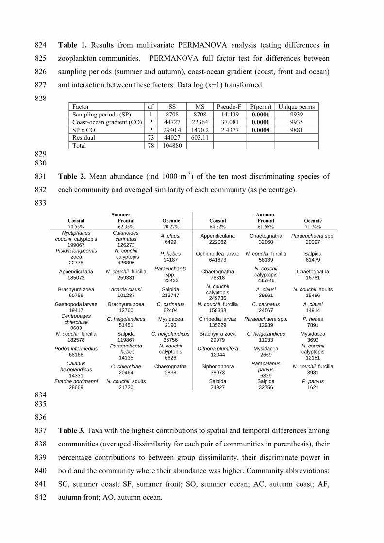
Table 1. Results from multivariate PERMANOVA analysis testing differences in
zooplankton communities. PERMANOVA full factor test for differences between
sampling periods (summer and autumn), coast-ocean gradient (coast, front and ocean)
and interaction between these factors. Data log (x+1) transformed.
824
825
826
827
828 Factor df SS MS Pseudo-F P(perm) Unique perms Sampling periods (SP) 1 8708 8708 14.439 0.0001 9939 Coast-ocean gradient (CO) 2 44727 22364 37.081 0.0001 9935 SP x CO 2 2940.4 1470.2 2.4377 0.0008 9881 Residual 73 44027 603.11 Total 78 104880
829 830
831
832
833
Table 2. Mean abundance (ind 1000 m-3) of the ten most discriminating species of
each community and averaged similarity of each community (as percentage).
Summer Autumn
Coastal 70.55%
Frontal 62.35%
Oceanic 70.27%
Coastal 64.82%
Frontal 61.66%
Oceanic 71.74%
Nyctiphanes couchii calyptopis
199067
Calanoides carinatus 126273
A. clausi 6499
Appendicularia 222062
Chaetognatha 32060
Paraeuchaeta spp. 20097
Pisidia longicornis zoea
22775
N. couchii calyptopis 426896
P. hebes 14187
Ophiuroidea larvae 641873
N. couchii furcilia 58139
Salpida 61479
Appendicularia 185072
N. couchii furcilia 259331
Paraeuchaeta spp.
23423
Chaetognatha 76318
N. couchii calyptopis
235948
Chaetognatha 16781
Brachyura zoea 60756
Acartia clausi 101237
Salpida 213747
N. couchii calyptopis
249736
A. clausi 39961
N. couchii adults 15486
Gastropoda larvae 19417
Brachyura zoea 12760
C. carinatus 62404
N. couchii furcilia 158338
C. carinatus 24567
A. clausi 14914
Centropages chierchiae
8683
C. helgolandicus 51451
Mysidacea 2190
Cirripedia larvae 135229
Paraeuchaeta spp. 12939
P. hebes 7891
N. couchii furcilia 182578
Salpida 119867
C. helgolandicus36756
Brachyura zoea 29979
C. helgolandicus 11233
Mysidacea 3692
Podon intermedius 68166
Paraeuchaeta hebes
14135
N. couchii calyptopis
6626
Oithona plumifera 12044
Mysidacea 2669
N. couchii calyptopis
12151 Calanus
helgolandicus 14331
C. chierchiae 20464
Chaetognatha 2838
Siphonophora 38073
Paracalanus parvus 6829
N. couchii furcilia 3981
Evadne nordmanni 28669
N. couchii adults 21720 Salpida
24927 Salpida 32756
P. parvus 1621
834 835
836
837
838
839
840
841
842
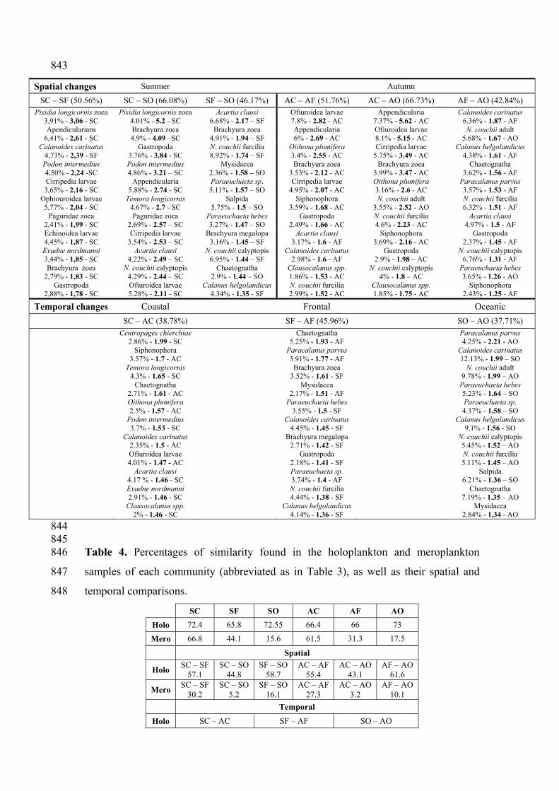
Table 3. Taxa with the highest contributions to spatial and temporal differences among
communities (averaged dissimilarity for each pair of communities in parenthesis), their
percentage contributions to between group dissimilarity, their discriminate power in
bold and the community where their abundance was higher. Community abbreviations:
SC, summer coast; SF, summer front; SO, summer ocean; AC, autumn coast; AF,
autumn front; AO, autumn ocean.
843
Spatial changes Summer Autumn
SC – SF (50.56%) SC – SO (66.08%) SF – SO (46.17%) AC – AF (51.76%) AC – AO (66.73%) AF – AO (42.84%) Pisidia longicornis zoea
3,91% - 3,06 - SC Pisidia longicornis zoea
4.01% - 5.2 - SC Acartia clausi
6.68% - 2.17 – SF Ofiuroidea larvae 7.8% - 2.82 - AC
Appendicularia 7.37% - 5.62 - AC
Calanoides carinatus 6.36% - 1.87 - AF
Apendicularians 6,41% - 2,61 - SC
Brachyura zoea 4.9% - 4.09 –SC
Brachyura zoea 4.91% - 1.94 – SF
Appendicularia 6% - 2.69 - AC
Ofiuroidea larvae 8.1% - 5.15 - AC
N. couchii adult 5.68% - 1.67 - AO
Calanoides carinatus 4,73% - 2,39 - SF
Gastropoda 3.76% - 3.84 - SC
N. couchii furcilia 8.92% - 1.74 – SF
Oithona plumifera 3.4% - 2.55 - AC
Cirripedia larvae 5.75% - 3.49 - AC
Calanus helgolandicus 4.38% - 1.61 - AF
Podon intermedius 4,50% - 2,24 -SC
Podon intermedius 4.86% - 3.21 – SC
Mysidacea 2.36% - 1.58 – SO
Brachyura zoea 3.53% - 2.12 - AC
Brachyura zoea 3.99% - 3.47 - AC
Chaetognatha 3.62% - 1.56 - AF
Cirripedia larvae 3,65% - 2,16 - SC
Appendicularia 5.88% - 2.74 - SC
Paraeuchaeta sp. 5.11% - 1.57 – SO
Cirripedia larvae 4.95% - 2.07 - AC
Oithona plumifera 3.16% - 2.6 - AC
Paracalanus parvus 3.57% - 1.53 - AF
Ophiouroidea larvae 5,77% - 2,04 - SC
Temora longicornis 4.67% - 2.7 - SC
Salpida 5.75% - 1.5 – SO
Siphonophora 3.59% - 1.68 - AC
N. couchii adult 3.55% - 2.52 - AO
N. couchii furcilia 6.32% - 1.51 - AF
Paguridae zoea 2,41% - 1,99 - SC
Paguridae zoea 2.69% - 2.57 – SC
Paraeuchaeta hebes 3.27% - 1.47 – SO
Gastropoda 2.49% - 1.66 - AC
N. couchii furcilia 4.6% - 2.23 - AC
Acartia clausi 4.97% - 1.5 - AF
Echinoidea larvae 4,45% - 1,87 - SC
Cirripedia larvae 3.54% - 2.53 – SC
Brachyura megalopa 3.16% - 1.45 – SF
Acartia clausi 3.17% - 1.6 - AF
Siphonophora 3.69% - 2.16 - AC
Gastropoda 2.37% - 1.45 - AF
Evadne nordmanni 3,44% - 1,85 - SC
Acartia clausi 4.22% - 2.49 – SC
N. couchii calyptopis 6.95% - 1.44 – SF
Calanoides carinatus 2.98% - 1.6 - AF
Gastropoda 2.9% - 1.98 – AC
N. couchii calyptopis 6.76% - 1.31 - AF
Brachyura zoea 2,79% - 1,83 - SC
N. couchii calyptopis 4.29% - 2.44 – SC
Chaetognatha 2.9% - 1.44 – SO
Clausocalanus spp. 1.86% - 1.53 - AC
N. couchii calyptopis 4% - 1.8 – AC
Paraeuchaeta hebes 3.65% - 1.26 - AO
Gastropoda 2,88% - 1,78 - SC
Ofiuroidea larvae 5.28% - 2.11 - SC
Calanus helgolandicus 4.34% - 1.35 - SF
N. couchii furcilia 2.99% - 1.52 - AC
Clausocalanus spp. 1.85% - 1.75 - AC
Siphonophora 2.43% - 1.25 - AF
Temporal changes Coastal Frontal Oceanic SC – AC (38.78%) SF – AF (45.96%) SO – AO (37.71%)
Centropages chierchiae
2.86% - 1.99 - SC Chaetognatha
5.25% - 1.93 - AF Paracalanus parvus 4.25% - 2.21 - AO
Siphonophora
3.57% - 1.7 - AC Paracalanus parvus 3.91% - 1.77 - AF
Calanoides carinatus 12.13% - 1.99 – SO
Temora longicornis
4.3% - 1.65 - SC Brachyura zoea
3.52% - 1.61 - SF N. couchii adult
9.78% - 1.99 – AO
Chaetognatha
2.71% - 1.61 - AC Mysidacea
2.17% - 1.51 - AF Paraeuchaeta hebes 5.23% - 1.64 – SO
Oithona plumifera 2.5% - 1.57 - AC
Paraeuchaeta hebes 3.55% - 1.5 - SF
Paraeuchaeta sp. 4.37% - 1.58 – SO
Podon intermedius 3.7% - 1.53 - SC
Calanoides carinatus 4.45% - 1.45 - SF
Calanus helgolandicus 9.1% - 1.56 - SO
Calanoides carinatus
2.35% - 1.5 - AC Brachyura megalopa
2.71% - 1.42 - SF N. couchii calyptopis 5.45% - 1.52 – AO
Ofiuroidea larvae 4.01% - 1.47 - AC
Gastropoda 2.18% - 1.41 - SF
N. couchii furcilia 5.11% - 1.45 – AO
Acartia clausi
4.17 % - 1.46 - SC Paraeuchaeta sp. 3.74% - 1.4 - AF
Salpida 6.21% - 1.36 – SO
Evadne nordmanni 2.91% - 1.46 - SC
N. couchii furcilia 4.44% - 1.38 - SF
Chaetognatha 7.19% - 1.35 – AO
Clausocalanus spp.
2% - 1.46 - SC Calanus helgolandicus
4.14% - 1.36 - SF Mysidacea
2.84% - 1.34 - AO
844 845 846
847
848
Table 4. Percentages of similarity found in the holoplankton and meroplankton
samples of each community (abbreviated as in Table 3), as well as their spatial and
temporal comparisons. SC SF SO AC AF AO
Holo 72.4 65.8 72.55 66.4 66 73
Mero 66.8 44.1 15.6 61.5 31.3 17.5
Spatial
Holo SC – SF 57.1
SC – SO 44.8
SF – SO 58.7
AC – AF 55.4
AC – AO 43.1
AF – AO 61.6
Mero SC – SF 30.2
SC – SO 5.2
SF – SO 16.1
AC – AF 27.3
AC – AO 3.2
AF – AO 10.1
Temporal
Holo SC – AC SF – AF SO – AO
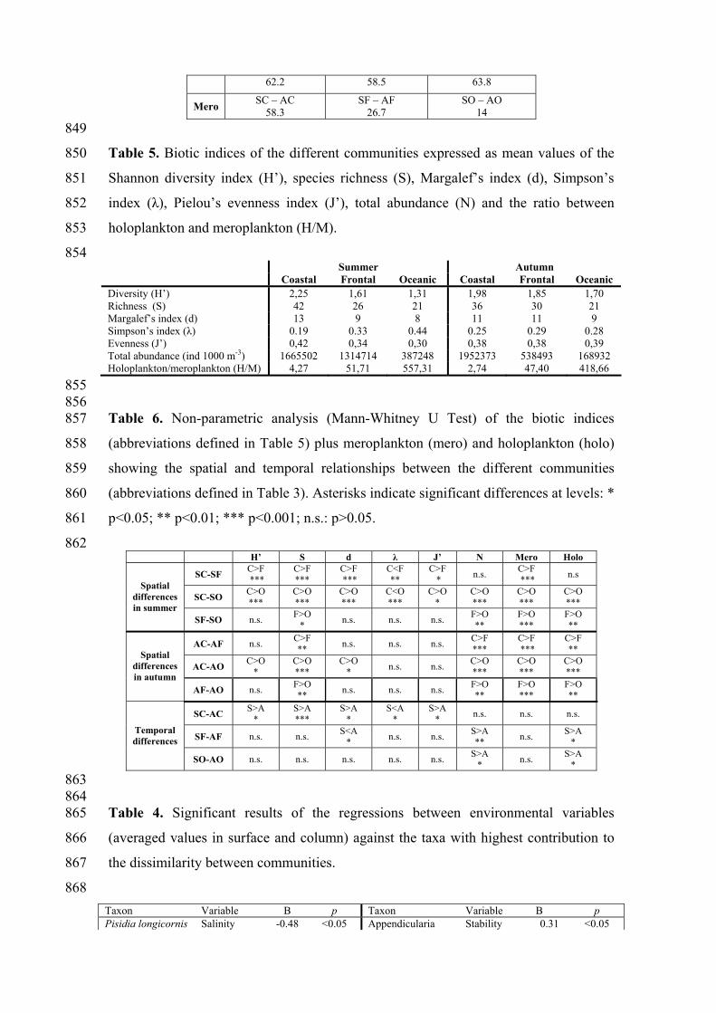
62.2 58.5 63.8
Mero SC – AC 58.3
SF – AF 26.7
SO – AO 14
849
850
851
852
853
854
Table 5. Biotic indices of the different communities expressed as mean values of the
Shannon diversity index (H’), species richness (S), Margalef’s index (d), Simpson’s
index (λ), Pielou’s evenness index (J’), total abundance (N) and the ratio between
holoplankton and meroplankton (H/M).
Summer Autumn Coastal Frontal Oceanic Coastal Frontal Oceanic Diversity (H’) 2,25 1,61 1,31 1,98 1,85 1,70 Richness (S) 42 26 21 36 30 21 Margalef’s index (d) 13 9 8 11 11 9 Simpson’s index (λ) 0.19 0.33 0.44 0.25 0.29 0.28 Evenness (J’) 0,42 0,34 0,30 0,38 0,38 0,39 Total abundance (ind 1000 m-3) 1665502 1314714 387248 1952373 538493 168932 Holoplankton/meroplankton (H/M) 4,27 51,71 557,31 2,74 47,40 418,66
855 856 857
858
859
860
861
862
Table 6. Non-parametric analysis (Mann-Whitney U Test) of the biotic indices
(abbreviations defined in Table 5) plus meroplankton (mero) and holoplankton (holo)
showing the spatial and temporal relationships between the different communities
(abbreviations defined in Table 3). Asterisks indicate significant differences at levels: *
p<0.05; ** p<0.01; *** p<0.001; n.s.: p>0.05.
H’ S d λ J’ N Mero Holo
SC-SF C>F ***
C>F ***
C>F ***
C<F **
C>F * n.s. C>F
*** n.s
SC-SO C>O ***
C>O ***
C>O ***
C<O ***
C>O *
C>O ***
C>O ***
C>O ***
Spatial differences in summer
SF-SO n.s. F>O * n.s. n.s. n.s. F>O
** F>O ***
F>O **
AC-AF n.s. C>F ** n.s. n.s. n.s. C>F
*** C>F ***
C>F **
AC-AO C>O *
C>O ***
C>O * n.s. n.s. C>O
*** C>O ***
C>O ***
Spatial differences in autumn
AF-AO n.s. F>O ** n.s. n.s. n.s. F>O
** F>O ***
F>O **
SC-AC S>A *
S>A ***
S>A *
S<A *
S>A * n.s. n.s. n.s.
SF-AF n.s. n.s. S<A * n.s. n.s. S>A
** n.s. S>A *
Temporal differences
SO-AO n.s. n.s. n.s. n.s. n.s. S>A * n.s. S>A
*
863 864 865
866
867
868
Table 4. Significant results of the regressions between environmental variables
(averaged values in surface and column) against the taxa with highest contribution to
the dissimilarity between communities.
Taxon Variable B p Taxon Variable B p Pisidia longicornis Salinity -0.48 <0.05 Appendicularia Stability 0.31 <0.05
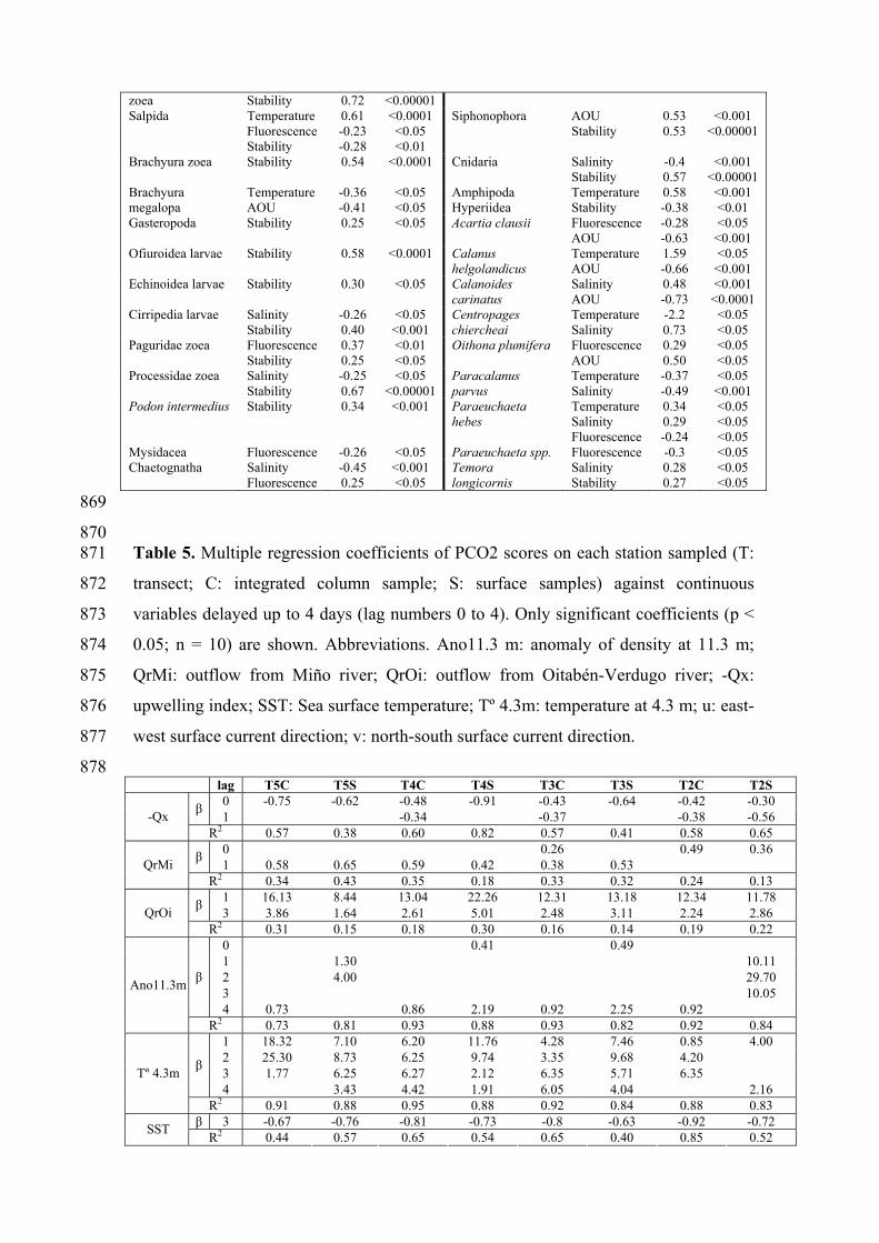
zoea Stability 0.72 <0.00001 Salpida Temperature
Fluorescence Stability
0.61 -0.23 -0.28
<0.0001 <0.05 <0.01
Siphonophora AOU Stability
0.53 0.53
<0.001 <0.00001
Brachyura zoea Stability 0.54 <0.0001 Cnidaria Salinity Stability
-0.4 0.57
<0.001 <0.00001
Brachyura megalopa
Temperature AOU
-0.36 -0.41
<0.05 <0.05
Amphipoda Hyperiidea
Temperature Stability
0.58 -0.38
<0.001 <0.01
Gasteropoda Stability 0.25 <0.05 Acartia clausii Fluorescence AOU
-0.28 -0.63
<0.05 <0.001
Ofiuroidea larvae Stability 0.58 <0.0001 Calanus helgolandicus
Temperature AOU
1.59 -0.66
<0.05 <0.001
Echinoidea larvae Stability 0.30 <0.05 Calanoides carinatus
Salinity AOU
0.48 -0.73
<0.001 <0.0001
Cirripedia larvae Salinity Stability
-0.26 0.40
<0.05 <0.001
Centropages chiercheai
Temperature Salinity
-2.2 0.73
<0.05 <0.05
Paguridae zoea Fluorescence Stability
0.37 0.25
<0.01 <0.05
Oithona plumifera Fluorescence AOU
0.29 0.50
<0.05 <0.05
Processidae zoea Salinity Stability
-0.25 0.67
<0.05 <0.00001
Paracalanus parvus
Temperature Salinity
-0.37 -0.49
<0.05 <0.001
Podon intermedius Stability 0.34 <0.001 Paraeuchaeta hebes
Temperature Salinity Fluorescence
0.34 0.29 -0.24
<0.05 <0.05 <0.05
Mysidacea Fluorescence -0.26 <0.05 Paraeuchaeta spp. Fluorescence -0.3 <0.05 Chaetognatha Salinity
Fluorescence -0.45 0.25
<0.001 <0.05
Temora longicornis
Salinity Stability
0.28 0.27
<0.05 <0.05
869
870 871
872
873
874
875
876
877
878
Table 5. Multiple regression coefficients of PCO2 scores on each station sampled (T:
transect; C: integrated column sample; S: surface samples) against continuous
variables delayed up to 4 days (lag numbers 0 to 4). Only significant coefficients (p <
0.05; n = 10) are shown. Abbreviations. Ano11.3 m: anomaly of density at 11.3 m;
QrMi: outflow from Miño river; QrOi: outflow from Oitabén-Verdugo river; -Qx:
upwelling index; SST: Sea surface temperature; Tº 4.3m: temperature at 4.3 m; u: east-
west surface current direction; v: north-south surface current direction.
lag T5C T5S T4C T4S T3C T3S T2C T2S
0 -0.75 -0.62 -0.48 -0.91 -0.43 -0.64 -0.42 -0.30 β 1 -0.34 -0.37 -0.38 -0.56 -Qx R2 0.57 0.38 0.60 0.82 0.57 0.41 0.58 0.65
0 0.26 0.49 0.36 β 1 0.58 0.65 0.59 0.42 0.38 0.53 QrMi R2 0.34 0.43 0.35 0.18 0.33 0.32 0.24 0.13
1 16.13 8.44 13.04 22.26 12.31 13.18 12.34 11.78 β 3 3.86 1.64 2.61 5.01 2.48 3.11 2.24 2.86 QrOi R2 0.31 0.15 0.18 0.30 0.16 0.14 0.19 0.22
0 0.41 0.49 1 1.30 10.11 2 4.00 29.70 3 10.05
β
4 0.73 0.86 2.19 0.92 2.25 0.92
Ano11.3m
R2 0.73 0.81 0.93 0.88 0.93 0.82 0.92 0.84 1 18.32 7.10 6.20 11.76 4.28 7.46 0.85 4.00 2 25.30 8.73 6.25 9.74 3.35 9.68 4.20 3 1.77 6.25 6.27 2.12 6.35 5.71 6.35 β
4 3.43 4.42 1.91 6.05 4.04 2.16 Tº 4.3m
R2 0.91 0.88 0.95 0.88 0.92 0.84 0.88 0.83 β 3 -0.67 -0.76 -0.81 -0.73 -0.8 -0.63 -0.92 -0.72 SST R2 0.44 0.57 0.65 0.54 0.65 0.40 0.85 0.52
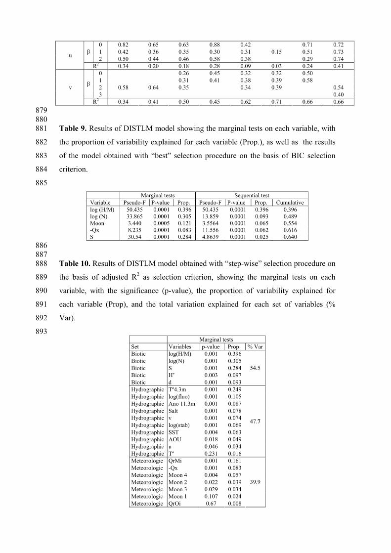
0 0.82 0.65 0.63 0.88 0.42 0.71 0.72 1 0.42 0.36 0.35 0.30 0.31 0.15 0.51 0.73 β 2 0.50 0.44 0.46 0.58 0.38 0.29 0.74 u
R2 0.34 0.20 0.18 0.28 0.09 0.03 0.24 0.41 0 0.26 0.45 0.32 0.32 0.50 1 0.31 0.41 0.38 0.39 0.58 2 0.58 0.64 0.35 0.34 0.39 0.54 β
3 0.40 v
R2 0.34 0.41 0.50 0.45 0.62 0.71 0.66 0.66 879
880 881
882
883
884
885
Table 9. Results of DISTLM model showing the marginal tests on each variable, with
the proportion of variability explained for each variable (Prop.), as well as the results
of the model obtained with “best” selection procedure on the basis of BIC selection
criterion.
Marginal tests Sequential test Variable Pseudo-F P-value Prop. Pseudo-F P-value Prop. Cumulative log (H/M) 50.435 0.0001 0.396 50.435 0.0001 0.396 0.396 log (N) 33.865 0.0001 0.305 13.859 0.0001 0.093 0.489 Moon 3.440 0.0005 0.121 3.5564 0.0001 0.065 0.554 -Qx 8.235 0.0001 0.083 11.556 0.0001 0.062 0.616 S 30.54 0.0001 0.284 4.8639 0.0001 0.025 0.640
886 887 888
889
890
891
892
893
Table 10. Results of DISTLM model obtained with “step-wise” selection procedure on
the basis of adjusted R2 as selection criterion, showing the marginal tests on each
variable, with the significance (p-value), the proportion of variability explained for
each variable (Prop), and the total variation explained for each set of variables (%
Var).
Marginal tests Set Variables p-value Prop % VarBiotic log(H/M) 0.001 0.396 Biotic log(N) 0.001 0.305 Biotic S 0.001 0.284 Biotic H’ 0.003 0.097 Biotic d 0.001 0.093
54.5
Hydrographic Tº4.3m 0.001 0.249 Hydrographic log(fluo) 0.001 0.105 Hydrographic Ano 11.3m 0.001 0.087 Hydrographic Salt 0.001 0.078 Hydrographic v 0.001 0.074 Hydrographic log(stab) 0.001 0.069 Hydrographic SST 0.004 0.063 Hydrographic AOU 0.018 0.049 Hydrographic u 0.046 0.034 Hydrographic Tº 0.231 0.016
47.7
Meteorologic QrMi 0.001 0.161 Meteorologic -Qx 0.001 0.083 Meteorologic Moon 4 0.004 0.057 Meteorologic Moon 2 0.022 0.039 Meteorologic Moon 3 0.029 0.034 Meteorologic Moon 1 0.107 0.024 Meteorologic QrOi 0.67 0.008
39.9
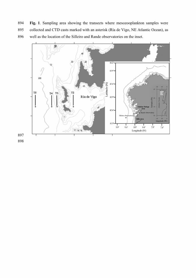
Fig. 1. Sampling area showing the transects where mesozooplankton samples were
collected and CTD casts marked with an asterisk (Ría de Vigo, NE Atlantic Ocean), as
well as the location of the Silleiro and Rande observatories on the inset.
894
895
896
897 898
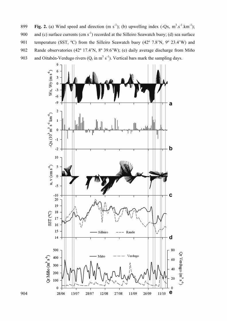
Fig. 2. (a) Wind speed and direction (m s-1); (b) upwelling index (-Qx, m3.s-1.km-1);
and (c) surface currents (cm s
899
900
901
902
903
-1) recorded at the Silleiro Seawatch buoy; (d) sea surface
temperature (SST, ºC) from the Silleiro Seawatch buoy (42º 7.8’N, 9º 23.4’W) and
Rande observatories (42º 17.4’N, 8º 39.6’W); (e) daily average discharge from Miño
and Oitabén-Verdugo rivers (Qr in m3 s-1). Vertical bars mark the sampling days.
904
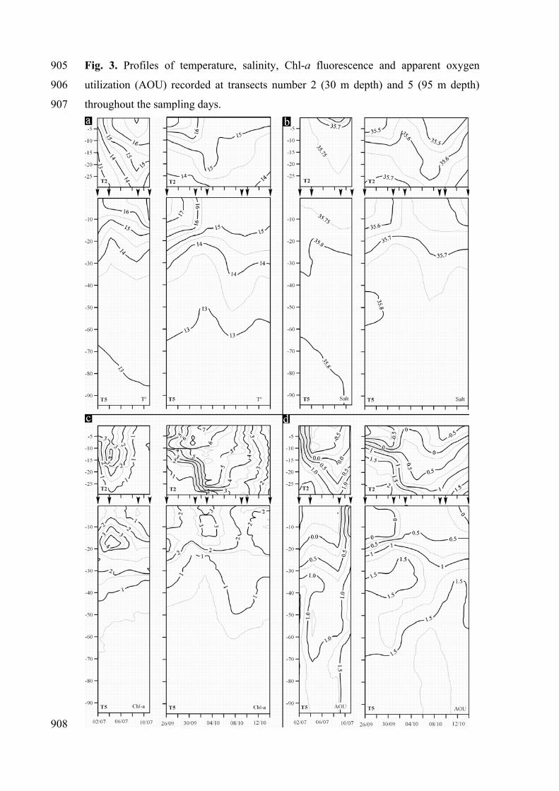
Fig. 3. Profiles of temperature, salinity, Chl-a fluorescence and apparent oxygen
utilization (AOU) recorded at transects number 2 (30 m depth) and 5 (95 m depth)
throughout the sampling days.
905
906
907
908
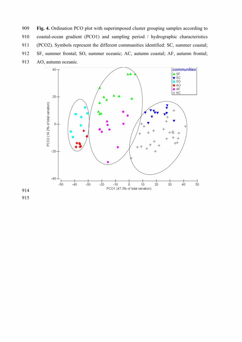
Fig. 4. Ordination PCO plot with superimposed cluster grouping samples according to
coastal-ocean gradient (PCO1) and sampling period / hydrographic characteristics
(PCO2). Symbols represent the different communities identified: SC, summer coastal;
SF, summer frontal; SO, summer oceanic; AC, autumn coastal; AF, autumn frontal;
AO, autumn oceanic.
909
910
911
912
913
914 915
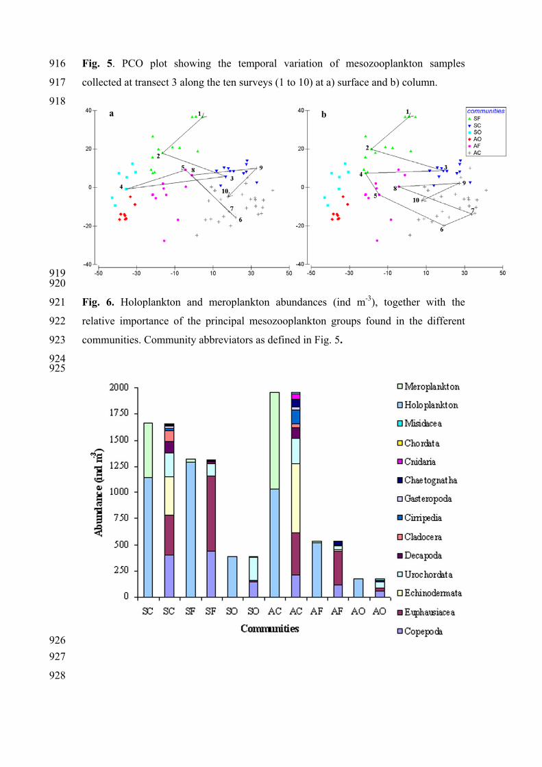
Fig. 5. PCO plot showing the temporal variation of mesozooplankton samples
collected at transect 3 along the ten surveys (1 to 10) at a) surface and b) column.
916
917
918
919 920
921
922
923
924 925
Fig. 6. Holoplankton and meroplankton abundances (ind m-3), together with the
relative importance of the principal mesozooplankton groups found in the different
communities. Community abbreviators as defined in Fig. 5.
926 927
928
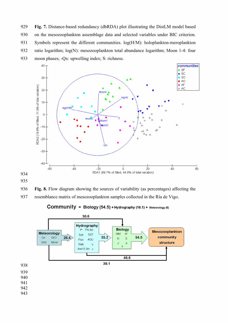
Fig. 7. Distance-based redundancy (dbRDA) plot illustrating the DistLM model based
on the mesozooplankton assemblage data and selected variables under BIC criterion.
Symbols represent the different communities. log(H/M): holoplankton-meroplankton
ratio logarithm; log(N): mesozooplankton total abundance logarithm; Moon 1-4: four
moon phases; -Qx: upwelling index; S: richness.
929
930
931
932
933
934 935
936
937
Fig. 8. Flow diagram showing the sources of variability (as percentages) affecting the
resemblance matrix of mesozooplankton samples collected in the Ría de Vigo.
938 939 940 941 942 943
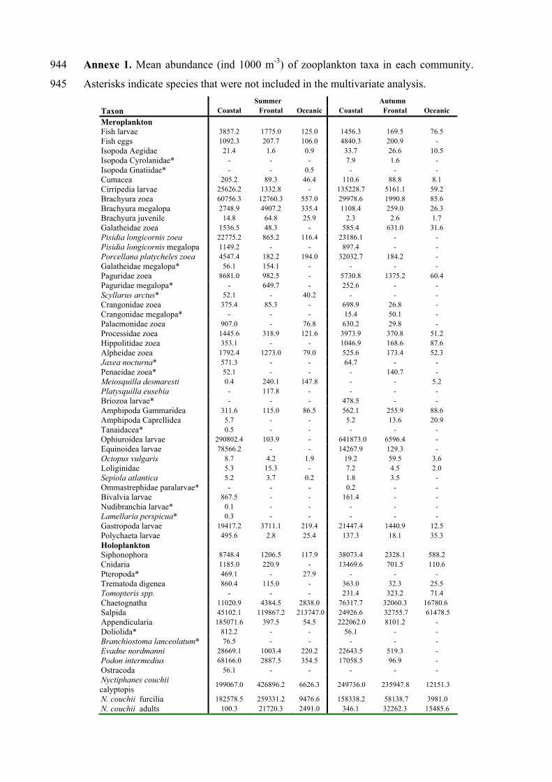
Annexe 1. Mean abundance (ind 1000 m-3) of zooplankton taxa in each community.
Asterisks indicate species that were not included in the multivariate analysis.
944
945 Summer Autumn
Taxon Coastal Frontal Oceanic Coastal Frontal Oceanic Meroplankton Fish larvae 3857.2 1775.0 125.0 1456.3 169.5 76.5 Fish eggs 1092.3 207.7 106.0 4840.3 200.9 - Isopoda Aegidae 21.4 1.6 0.9 33.7 26.6 10.5 Isopoda Cyrolanidae* - - - 7.9 1.6 - Isopoda Gnatiidae* - - 0.5 - - - Cumacea 205.2 89.3 46.4 110.6 88.8 8.1 Cirripedia larvae 25626.2 1332.8 - 135228.7 5161.1 59.2 Brachyura zoea 60756.3 12760.3 557.0 29978.6 1990.8 85.6 Brachyura megalopa 2748.9 4907.2 335.4 1108.4 259.0 26.3 Brachyura juvenile 14.8 64.8 25.9 2.3 2.6 1.7 Galatheidae zoea 1536.5 48.3 - 585.4 631.0 31.6 Pisidia longicornis zoea 22775.2 865.2 116.4 23186.1 - - Pisidia longicornis megalopa 1149.2 - - 897.4 - - Porcellana platycheles zoea 4547.4 182.2 194.0 32032.7 184.2 - Galatheidae megalopa* 56.1 154.1 - - - - Paguridae zoea 8681.0 982.5 - 5730.8 1375.2 60.4 Paguridae megalopa* - 649.7 - 252.6 - - Scyllarus arctus* 52.1 - 40.2 - - - Crangonidae zoea 375.4 85.3 - 698.9 26.8 - Crangonidae megalopa* - - - 15.4 50.1 - Palaemonidae zoea 907.0 - 76.8 630.2 29.8 - Processidae zoea 1445.6 318.9 121.6 3973.9 370.8 51.2 Hippolitidae zoea 353.1 - - 1046.9 168.6 87.6 Alpheidae zoea 1792.4 1273.0 79.0 525.6 173.4 52.3 Jaxea nocturna* 571.3 - - 64.7 - - Penaeidae zoea* 52.1 - - - 140.7 - Meiosquilla desmaresti 0.4 240.1 147.8 - - 5.2 Platysquilla eusebia - 117.8 - - - - Briozoa larvae* - - - 478.5 - - Amphipoda Gammaridea 311.6 115.0 86.5 562.1 255.9 88.6 Amphipoda Caprellidea 5.7 - - 5.2 13.6 20.9 Tanaidacea* 0.5 - - - - - Ophiuroidea larvae 290802.4 103.9 - 641873.0 6596.4 - Equinoidea larvae 78566.2 - - 14267.9 129.3 - Octopus vulgaris 8.7 4.2 1.9 19.2 59.5 3.6 Loliginidae 5.3 15.3 - 7.2 4.5 2.0 Sepiola atlantica 5.2 3.7 0.2 1.8 3.5 - Ommastrephidae paralarvae* - - - 0.2 - - Bivalvia larvae 867.5 - - 161.4 - - Nudibranchia larvae* 0.1 - - - - - Lamellaria perspicua* 0.3 - - - - - Gastropoda larvae 19417.2 3711.1 219.4 21447.4 1440.9 12.5 Polychaeta larvae 495.6 2.8 25.4 137.3 18.1 35.3 Holoplankton Siphonophora 8748.4 1206.5 117.9 38073.4 2328.1 588.2 Cnidaria 1185.0 220.9 - 13469.6 701.5 110.6 Pteropoda* 469.1 - 27.9 - - - Trematoda digenea 860.4 115.0 - 363.0 32.3 25.5 Tomopteris spp. - - - 231.4 323.2 71.4 Chaetognatha 11020.9 4384.5 2838.0 76317.7 32060.3 16780.6 Salpida 45102.1 119867.2 213747.0 24926.6 32755.7 61478.5 Appendicularia 185071.6 397.5 54.5 222062.0 8101.2 - Doliolida* 812.2 - - 56.1 - - Branchiostoma lanceolatum* 76.5 - - - - - Evadne nordmanni 28669.1 1003.4 220.2 22643.5 519.3 - Podon intermedius 68166.0 2887.5 354.5 17058.5 96.9 - Ostracoda 56.1 - - - - - Nyctiphanes couchii calyptopis 199067.0 426896.2 6626.3 249736.0 235947.8 12151.3
N. couchii furcilia 182578.5 259331.2 9476.6 158338.2 58138.7 3981.0 N. couchii adults 100.3 21720.3 2491.0 346.1 32262.3 15485.6
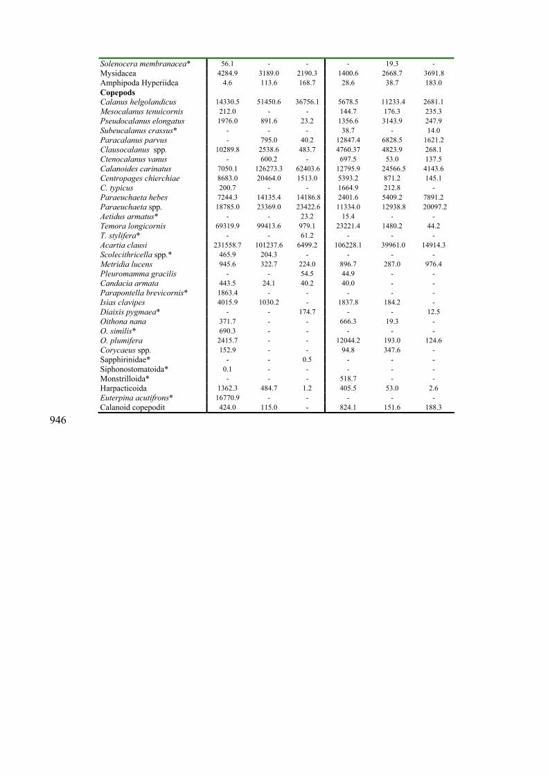
Solenocera membranacea* 56.1 - - - 19.3 - Mysidacea 4284.9 3189.0 2190.3 1400.6 2668.7 3691.8 Amphipoda Hyperiidea 4.6 113.6 168.7 28.6 38.7 183.0 Copepods Calanus helgolandicus 14330.5 51450.6 36756.1 5678.5 11233.4 2681.1 Mesocalanus tenuicornis 212.0 - - 144.7 176.3 235.3 Pseudocalanus elongatus 1976.0 891.6 23.2 1356.6 3143.9 247.9 Subeucalanus crassus* - - - 38.7 - 14.0 Paracalanus parvus - 795.0 40.2 12847.4 6828.5 1621.2 Clausocalanus spp. 10289.8 2538.6 483.7 4760.37 4823.9 268.1 Ctenocalanus vanus - 600.2 - 697.5 53.0 137.5 Calanoides carinatus 7050.1 126273.3 62403.6 12795.9 24566.5 4143.6 Centropages chierchiae 8683.0 20464.0 1513.0 5393.2 871.2 145.1 C. typicus 200.7 - - 1664.9 212.8 - Paraeuchaeta hebes 7244.3 14135.4 14186.8 2401.6 5409.2 7891.2 Paraeuchaeta spp. 18785.0 23369.0 23422.6 11334.0 12938.8 20097.2 Aetidus armatus* - - 23.2 15.4 - - Temora longicornis 69319.9 99413.6 979.1 23221.4 1480.2 44.2 T. stylifera* - - 61.2 - - - Acartia clausi 231558.7 101237.6 6499.2 106228.1 39961.0 14914.3 Scolecithricella spp.* 465.9 204.3 - - - - Metridia lucens 945.6 322.7 224.0 896.7 287.0 976.4 Pleuromamma gracilis - - 54.5 44.9 - - Candacia armata 443.5 24.1 40.2 40.0 - - Parapontella brevicornis* 1863.4 - - - - - Isias clavipes 4015.9 1030.2 - 1837.8 184.2 - Diaixis pygmaea* - - 174.7 - - 12.5 Oithona nana 371.7 - - 666.3 19.3 - O. similis* 690.3 - - - - - O. plumifera 2415.7 - - 12044.2 193.0 124.6 Corycaeus spp. 152.9 - - 94.8 347.6 - Sapphirinidae* - - 0.5 - - - Siphonostomatoida* 0.1 - - - - - Monstrilloida* - - - 518.7 - - Harpacticoida 1362.3 484.7 1.2 405.5 53.0 2.6 Euterpina acutifrons* 16770.9 - - - - - Calanoid copepodit 424.0 115.0 - 824.1 151.6 188.3
946


