Download - Seismic Hazard Assessment: Issues and AlternativesSeismic Hazard Assessment: Issues and Alternatives ZHENMING WANG 1 Abstract—Seismic hazard and risk are two very important concepts

Seismic Hazard Assessment: Issues and Alternatives

ZHENMING WANG1

Abstract—Seismic hazard and risk are two very important

concepts in engineering design and other policy considerations.

Although seismic hazard and risk have often been used inter-

changeably, they are fundamentally different. Furthermore, seismic

risk is more important in engineering design and other policy

considerations. Seismic hazard assessment is an effort by earth

scientists to quantify seismic hazard and its associated uncertainty

in time and space and to provide seismic hazard estimates for

seismic risk assessment and other applications. Although seismic

hazard assessment is more a scientific issue, it deserves special

attention because of its significant implication to society. Two

approaches, probabilistic seismic hazard analysis (PSHA) and

deterministic seismic hazard analysis (DSHA), are commonly used

for seismic hazard assessment. Although PSHA has been pro-

claimed as the best approach for seismic hazard assessment, it is

scientifically flawed (i.e., the physics and mathematics that PSHA

is based on are not valid). Use of PSHA could lead to either unsafe

or overly conservative engineering design or public policy, each of

which has dire consequences to society. On the other hand, DSHA

is a viable approach for seismic hazard assessment even though it

has been labeled as unreliable. The biggest drawback of DSHA is

that the temporal characteristics (i.e., earthquake frequency of

occurrence and the associated uncertainty) are often neglected. An

alternative, seismic hazard analysis (SHA), utilizes earthquake

science and statistics directly and provides a seismic hazard esti-

mate that can be readily used for seismic risk assessment and other

applications.

1. Introduction

It is a daunting task to try to convey the science of

seismology/geology to engineers, policy-makers, and

the general public. It is essential to make every effort

to convey the science clearly, accurately, and

understandably because science is the basis for sound

engineering design and other policy considerations.

This is also the duty of professional seismologists/

geologists.

It is often heard, ‘‘I am just a seismologist (or

geologist) and this is what it is.’’ It is also often heard,

‘‘The selection of an appropriate seismic hazard or

risk for engineering design or policy consideration is

not really a technical question, but rather a societal

one.’’ Clearly, there is a gap in understanding of

seismic hazard and risk between the seismologists/

geologists who assess them and engineers, policy-

makers, and the general public who use these

assessments. For example, the national seismic haz-

ard maps produced by the U.S. Geological Survey

using probabilistic seismic hazard analysis (PSHA),

and showing the ground motions with 2, 5, and 10%

probability of exceedance (PE) in 50 years, have

been said to be the hazard maps that engineers want

(FRANKEL et al., 1996, 2000, 2002; PETERSEN et al.,

2008). By definition, ground motions with 2, 5, and

10% PE in 50 years represent seismic risk in a

manner similar to flood and wind risk estimates in

hydraulic and wind engineering (SACHS, 1978; GUPTA,

1989); but engineers may be using the national seis-

mic hazard maps only because they represent the

‘‘best available science’’ (BSSC, 1998; LEYENDECKER

et al., 2000). Although it has been claimed that the

national seismic hazard maps have been used in a

variety of engineering designs, such as the Interna-

tional Building Code (ICC, 2006), the fact is that the

USGS hazard maps have never been used directly in

building design, and ‘‘the 2008 national seismic

hazard maps should not be substituted for the model

building code design maps nor should they be used

with ASCE/SEI 41 or 31 for seismic rehabilitation or

evaluation’’ (USGS, 2009). The gap in understanding

of the national seismic hazard maps has made it

difficult to use them for engineering design and other

policy considerations in many communities in the

1 Kentucky Geological Survey, University of Kentucky,

228 Mining and Mineral Resources Building, Lexington, KY

40506, USA. E-mail: [email protected]

Pure Appl. Geophys.

� 2010 Springer Basel AG

DOI 10.1007/s00024-010-0148-3 Pure and Applied Geophysics

central and eastern United States (STEIN et al., 2003;

WANG et al., 2003).

This paper examines the basic concepts of seismic

hazard and risk first, because they are two important

parameters for engineering design and policy consid-

eration. The methodologies used to assess seismic

hazard, as well as the associated science, will then be

explored. The goal of this paper is to bridge the gap in

understanding of seismic hazard and risk, as well as the

associated science, between seismologists/geologists,

engineers, policy-makers, and the general public, with

the aim of achieving seismically safe and resilient

communities.

2. Seismic Hazard and Risk

2.1. Basic Concept

Seismic hazard and risk are two of the most

commonly used terms in engineering design and policy

considerations. Although the two terms have often been

used interchangeably, they are fundamentally different

concepts (REITER, 1990; WANG, 2006, 2007, 2009b).

Seismic hazards are defined as ‘‘the potential for

dangerous, earthquake-related natural phenomena such

as ground shaking, fault rupture, or soil liquefaction’’

(REITER, 1990, p. 3), or ‘‘a property of an earthquake that

can cause damage and loss’’ (MCGUIRE, 2004, p. 7).

Seismic risk is defined as ‘‘the probability of occurrence

of these consequences (i.e., adverse consequences to

society such as the destruction of buildings or the loss of

life that could result from seismic hazards)’’ (REITER,

1990, p. 3), or ‘‘the probability that some humans will

incur loss or that their built environment will be

damaged’’ (MCGUIRE, 2004, p. 8). In other words,

seismic hazard describes the natural phenomenon or

property of an earthquake, whereas seismic risk

describes the probability of loss or damage that could

be caused by a seismic hazard (WANG, 2009b). This

difference is illustrated in Fig. 1, which shows that the

Wenchuan earthquake and its aftershocks triggered

massive landslides and rockfalls (seismic hazards). The

driver and pedestrians shown in Fig. 1, who were

vulnerable to the seismic hazards, were taking a risk, the

probability of an adverse consequence: being struck by a

rockfall. This example demonstrates that seismic risk is

a probable outcome (or consequence) from interaction

between a seismic hazard and vulnerability (something

is vulnerable to the seismic hazard). Therefore, in

general, seismic risk can be expressed qualitatively as

Seismic risk ¼ Seismic hazardHVulnerability: ð1Þ

As shown in Eq. 1, high seismic hazard does not

necessary mean high seismic risk, and vice versa.

Figure 1Comparison of seismic hazard and risk. Seismic hazard: earthquake triggered rockfall. Vulnerability: car, its driver, and pedestrians.

Consequence: struck by a rockfall. Seismic risk: the probability of being struck by a rockfall during the period that the car or pedestrians pass

through the road section

Z. Wang Pure Appl. Geophys.

There is no risk (i.e., no probability that the car or

pedestrians could be hit by a rockfall) if the driver

decides not to drive or pedestrians decide not to go

through the road (i.e., no vulnerability). This example

also demonstrates that engineering design or a policy

for seismic hazard mitigation may differ from one for

seismic risk reduction. Here, the seismic hazard

(rockfall) may or may not be mitigated, but the

seismic risk can always be reduced by either

mitigating the seismic hazard (i.e., building barriers

and other measures), reducing the vulnerability (i.e.,

limiting traffic or pedestrians), or both. Therefore, it

is critical for engineers and decision-makers to

clearly understand seismic hazard and risk.

2.2. Estimations

The preceding discussions on seismic hazard and

risk are in general, or qualitative, terms, which is

insufficient for decision-making. As natural phenom-

enon, seismic hazard is quantitatively defined

by three parameters: level of severity (physical

measurement), spatial measurement (where), and

temporal measurement (when or how often), as well

as associated uncertainties. For example, the hazard

in Fig. 1 can be quantified as a rockfall with a mean

diameter of 0.5 m or larger that occurs every hour on

average along the section of the road. Seismic

hazards can also be quantified as an M7.5 earthquake

(mean) with a recurrence interval of 500 years

(mean) in the New Madrid Seismic Zone of the

central United States, or a mean peak ground

acceleration (PGA) of 0.3 g with a mean return

period of 1,000 years in Memphis, TN. Seismic

hazard is assessed from instrumental, historical, and

geological observations. In other words, seismic

hazard is assessed from earth sciences. How to assess

seismic hazard will be discussed in detail later.

Seismic risk quantification is complicated and

somewhat subjective because it depends on the desired

measurement of consequence (i.e., outcome of phys-

ical interaction between the seismic hazard and

vulnerability) and how the hazard and vulnerability

interact in time and space. The hazard and vulnerability

could interact at a specific site or over an area: so-called

site-specific risk or aggregate risk (MALHOTRA, 2008).

In general, seismic risk is quantified by four

parameters: probability, level of severity, and spatial

and temporal measurements (WANG, 2009b). For

example, the Working Group on California Earthquake

Probabilities (WGCEP, 2003) estimated that ‘‘there is a

62 percent probability of a major, damaging earth-

quake (M6.7 or greater) striking the greater San

Francisco Bay Region (SFBR) over the next 30 years

(2002–2031).’’ The October 17, 1989, Loma Prieta

earthquake (M6.9) caused 62 deaths, about 4,000

injuries, and $10 billion in direct losses in the SFBR.

Thus, the risk, in terms of an earthquake of M6.7 or

greater, could also be expressed as a 62% probability of

60 or more deaths, 4,000 or more injuries, or $10 bil-

lion or more in direct losses over the next 30 years.

These risk estimates are from all sources for an area

such as SFBR. For an individual site or source, the risk

estimate could be different. WGCEP (2003) estimated

the risk in terms of modified Mercalli intensity (MMI);

for example, the MMI of shaking at a given site with a

50% chance of being exceeded in 30 years. WGCEP

(2003) estimated that in Oakland, CA, there is an 11%

probability of an earthquake with M6.7 or greater

occurring on the southern Hayward Fault over the next

30 years. WGCEP’s work shows that seismic risk

estimate is very complicated and can be expressed in

many different ways for different users.

In order to estimate seismic risk, a model has to

be assumed or introduced to describe how the hazard

and vulnerability interact in time. For example,

several models (Poisson, Empirical, Brownian Pas-

sage Time, and Time-Predictable) have been used to

describe earthquake occurrence in time and to

estimate seismic risk. The most commonly used one

in seismic risk estimation is the Poisson model

(CORNELL, 1968; WGCEP, 2003). If earthquake

occurrence in time follows a Poisson distribution

(CORNELL, 1968; WANG, 2006, 2007), then seismic

risk, expressed in terms of the probability of an

earthquake exceeding a specified magnitude (M) at

least once during a given exposure time t for a given

vulnerability along a fault or in an area, can be

estimated by

p n� 1; t; sð Þ ¼ 1� e�t=s; ð2Þ

where n and s are the number and average recurrence

interval of an earthquake with magnitude exceeding

M. Equation 2 describes a quantitative relationship


between seismic hazard (i.e., an earthquake of

magnitude M or larger with an average recurrence

interval s) and seismic risk (i.e., the probability p that

an earthquake of magnitude M or larger could occur

during the exposure time t in the area), assuming that

earthquake occurrence in time follows a Poisson

distribution. The seismic risk estimate will be dif-

ferent if earthquake occurrence follows another

distribution. Equation 2 can be used to estimate

seismic risk for the car and pedestrians shown in

Fig. 1. For the given seismic hazard, a rockfall with a

mean diameter of 0.5 m or larger has a frequency of

occurrence of one every hour on average along that

section of the road. If it takes 3 min for the car to pass

through the road section, and 20 min for the pedes-

trians, the risk for the car will be about a 5%

probability of being struck by a rockfall with a

diameter of 0.5 m or larger; for the pedestrians, about

a 28% probability. The pedestrians will almost cer-

tainly be killed if they are struck by a rockfall of

0.5 m or larger in diameter, but the driver of the car

may not be killed if the car is struck by a similar

rockfall, because the body of the car could protect the

driver. Thus, we assume that pedestrians will be

killed (100% chance) if they are struck by a rockfall

and that there is a 30% chance that the driver will be

killed if the car is struck by a similar rockfall. The

pedestrians have about a 28% probability of being

killed, and the driver has about a 1.5% probability.

These examples demonstrate that (1) time is a key

element in risk estimation and (2) differences in

physical characteristics of the vulnerabilities, i.e., the

human body versus car or human body inside the car,

result in different seismic risk estimation. The human

body is more vulnerable to the rockfall hazard than

the one inside the car. The car could be damaged, but

the driver might not be injured if a rockfall struck the

car.

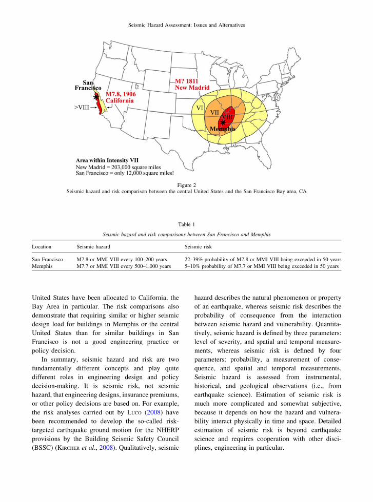
The quantitative relationship between seismic

hazard, vulnerability, and risk, as well as their roles

in engineering design and policy considerations, can

be illustrated through the following example. Fig-

ure 2 shows the modified Mercalli intensity

experienced during the 1906 San Francisco earth-

quake (M7.8) in the Bay Area and the 1811–1812

New Madrid earthquake (M7.7) in the central United

States. A much larger area was impacted by a similar

earthquake in the central United States than in

California because ground motion attenuates much

slower in the older and harder rock in the central

United States. In other words, a much larger area

experienced a similar MMI in the central United

States than in California. This does not mean that the

central United States has higher seismic hazard,

however, because the earthquake frequencies of

occurrence are different. The frequency of occurrence

of the M7.8 earthquake in the Bay Area is about

100–200 years, and about 500–1,000 years in the

central United States. As shown in Fig. 2, in terms of

seismic hazard, the Bay Area experienced either

an M7.8 earthquake or an MMI VIII every

100–200 years, whereas the central United States

experienced a similar earthquake or intensity every

500–1,000 years. It is not straight forward to make a

decision whether to spend more resources for seismic

hazard mitigation in the Bay Area or the central

United States based on these seismic hazard compar-

isons (Table 1).

Now, let’s consider seismic risk for two identical

buildings with a normal life of 50 years, one in San

Francisco and one in Memphis (Fig. 2). If the

earthquake occurrences follow a Poisson distribution,

we can use Eq. 2 to estimate seismic risk in terms of

the probability that the buildings could be hit by an

M7.8 earthquake or experience MMI VIII during

their 50 year lifespan. According to Eq. 2, the

probability of the building in San Francisco being

hit by an M7.8 earthquake or experiencing an MMI

VIII will be about 22–39% during its 50 year life; the

probability of the building in Memphis being hit by a

similar earthquake or experiencing a similar MMI

will be about 5–10% (Table 1). A recent study

(KIRCHER et al., 2006) shows that a repeat of the 1906

San Francisco earthquake (M7.8) could cause more

than $150 billion in losses in the Bay Area. A similar

size earthquake (M7.7) in the New Madrid Seismic

Zone could also cause huge losses in the central

United States, but the losses there would not be as

large as in the Bay Area because the vulnerabilities

(i.e., people and the built environments) are much

higher in the Bay Area than in the central United

States. The seismic risk comparisons (Table 1) make

it easy to understand why the most resources for

seismic hazard mitigation and risk reduction in the


United States have been allocated to California, the

Bay Area in particular. The risk comparisons also

demonstrate that requiring similar or higher seismic

design load for buildings in Memphis or the central

United States than for similar buildings in San

Francisco is not a good engineering practice or

policy decision.

In summary, seismic hazard and risk are two

fundamentally different concepts and play quite

different roles in engineering design and policy

decision-making. It is seismic risk, not seismic

hazard, that engineering designs, insurance premiums,

or other policy decisions are based on. For example,

the risk analyses carried out by LUCO (2008) have

been recommended to develop the so-called risk-

targeted earthquake ground motion for the NHERP

provisions by the Building Seismic Safety Council

(BSSC) (KIRCHER et al., 2008). Qualitatively, seismic

hazard describes the natural phenomenon or property

of an earthquake, whereas seismic risk describes the

probability of consequence from the interaction

between seismic hazard and vulnerability. Quantita-

tively, seismic hazard is defined by three parameters:

level of severity, and spatial and temporal measure-

ments, whereas seismic risk is defined by four

parameters: probability, a measurement of conse-

quence, and spatial and temporal measurements.

Seismic hazard is assessed from instrumental,

historical, and geological observations (i.e., from

earthquake science). Estimation of seismic risk is

much more complicated and somewhat subjective,

because it depends on how the hazard and vulnera-

bility interact physically in time and space. Detailed

estimation of seismic risk is beyond earthquake

science and requires cooperation with other disci-

plines, engineering in particular.

Figure 2Seismic hazard and risk comparison between the central United States and the San Francisco Bay area, CA

Table 1

Seismic hazard and risk comparisons between San Francisco and Memphis

Location Seismic hazard Seismic risk

San Francisco M7.8 or MMI VIII every 100–200 years 22–39% probability of M7.8 or MMI VIII being exceeded in 50 years

Memphis M7.7 or MMI VIII every 500–1,000 years 5–10% probability of M7.7 or MMI VIII being exceeded in 50 years


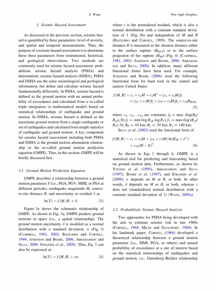
3. Seismic Hazard Assessment

As discussed in the previous section, seismic haz-

ard is quantified by three parameters: level of severity,

and spatial and temporal measurements. Thus, the

purpose of a seismic hazard assessment is to determine

these three parameters from instrumental, historical,

and geological observations. Two methods are

commonly used for seismic hazard assessment: prob-

abilistic seismic hazard analysis (PSHA) and

deterministic seismic hazard analysis (DSHA). PSHA

and DSHA use the same seismological and geological

information, but define and calculate seismic hazard

fundamentally differently. In PSHA, seismic hazard is

defined as the ground motion with an annual proba-

bility of exceedance and calculated from a so-called

triple integration (a mathematical model) based on

statistical relationships of earthquake and ground

motion. In DSHA, seismic hazard is defined as the

maximum ground motion from a single earthquake or

set of earthquakes and calculated from simple statistics

of earthquake and ground motion. A key component

for seismic hazard assessment including both PSHA

and DSHA is the ground motion attenuation relation-

ship or the so-called ground motion prediction

equation (GMPE). Thus, in this section, GMPE will be

briefly discussed first.

3.1. Ground Motion Prediction Equation

GMPE describes a relationship between a ground

motion parameter Y (i.e., PGA, PGV, MMI, or PSA at

different periods), earthquake magnitude M, source-

to-site distance R, and uncertainty or residual d as

lnðYÞ ¼ f ðM;RÞ þ d: ð3Þ

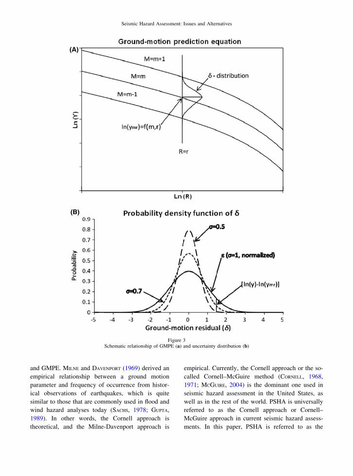
Figure 3a shows the schematic relationship of

GMPE. As shown in Fig. 3a, GMPE predicts ground

motions in space (i.e., a spatial relationship). The

ground motion uncertainty d is modeled as a normal

distribution with a standard deviation, r (Fig. 3)

(CAMPBELL, 1981, 2003; BAZZURRO and CORNELL,

1999; ATKINSON and BOORE, 2006; ABRAHAMSON and

SILVA, 2008; STRASSER et al., 2009). Thus, Eq. 3 can

also be expressed as

lnðYÞ ¼ f ðM;RÞ þ er; ð4Þ

where e is the normalized residual, which is also a

normal distribution with a constant standard devia-

tion of 1 (Fig. 3b) and independent of M and R

(BAZZURRO and CORNELL, 1999). The source-to-site

distance R is measured as the shortest distance either

to the surface rupture (RRUP) or to the surface

projection of the rupture (RJB) (Fig. 4) (CAMPBELL,

1981, 2003; ATKINSON and BOORE, 2006; ABRAHAM-

SON and SILVA, 2008). In addition, many different

functional forms have been used. For example,

ATKINSON and BOORE (2006) used the following

functional form for hard rock in the central and

eastern United States:

f ðM;RÞ ¼ c1þ c2Mþ c3M2þ ðc4þ c5MÞf1

þ ðc6þ c7MÞf2þ ðc8þ c9MÞf0þ c10RRUB;

ð5Þ

where c1, c2,…c10 are constants; f0 = max (log(R0/

Rcd), 0); f1 = min (log Rcd, log R1); f2 = max (log (Rcd/

R2), 0); R0 = 10 km; R1 = 70 km; R2 = 140 km.

SILVA et al. (2002) used the functional form of

f ðM;RÞ ¼ c1 þ c2M þ ðc6 þ c7MÞ ln RJB þ ec4ð Þþ c10ðM � 6Þ2: ð6Þ

As shown in Eqs. 3 through 6, GMPE is a

statistical tool for predicting and forecasting based

on ground motion data. Furthermore, as shown by

YOUNGS et al. (1995), ABRAHAMSON and SILVA

(1997), BOORE et al. (1997), and STRASSER et al.

(2009), r depends on M or R, or both. In other

words, d depends on M or R, or both, whereas edoes not (standardized normal distribution with a

constant standard deviation of 1) (WANG, 2009a).

3.2. Probabilistic Seismic Hazard Analysis

Two approaches for PSHA being developed with

the aim to estimate seismic risk in late 1960s

(CORNELL, 1968; MILNE and DAVENPORT, 1969). In

his landmark paper, CORNELL (1968) developed a

theoretical relationship between a ground motion

parameter (i.e., MMI, PGA, or others) and annual

probability of exceedance at a site of interest based

on the statistical relationships of earthquakes and

ground motion, i.e., Gutenberg–Richter relationship


and GMPE. MILNE and DAVENPORT (1969) derived an

empirical relationship between a ground motion

parameter and frequency of occurrence from histor-

ical observations of earthquakes, which is quite

similar to those that are commonly used in flood and

wind hazard analyses today (SACHS, 1978; GUPTA,

1989). In other words, the Cornell approach is

theoretical, and the Milne-Davenport approach is

empirical. Currently, the Cornell approach or the so-

called Cornell–McGuire method (CORNELL, 1968,

1971; MCGUIRE, 2004) is the dominant one used in

seismic hazard assessment in the United States, as

well as in the rest of the world. PSHA is universally

referred to as the Cornell approach or Cornell–

McGuire approach in current seismic hazard assess-

ments. In this paper, PSHA is referred to as the

Figure 3Schematic relationship of GMPE (a) and uncertainty distribution (b)


Cornell approach or so-called Cornell–McGuire

method.

PSHA was developed from earthquake science in

the 1970s under three fundamental assumptions: (a)

equal likelihood of earthquake occurrence (single

point) along a line or over an areal source, (b)

constant-in-time average occurrence rate of earth-

quakes, and (c) Poisson (or ‘‘memory-less’’) behavior

of earthquake occurrences (CORNELL 1968, 1971). It is

very important to note that the basic equation for

PSHA was derived from mathematical statistics.

According to mathematical statistics (BENJAMIN and

CORNELL, 1970; MENDENHALL et al., 1986; WANG and

ZHOU, 2007), if and only if M, R, and d are

independent random variables, the joint probability

density function for GMPE, Eq. 3, is

fM;R;Dðm; r; eÞ ¼ fMðmÞfRðrÞfDðdÞ; ð7Þ

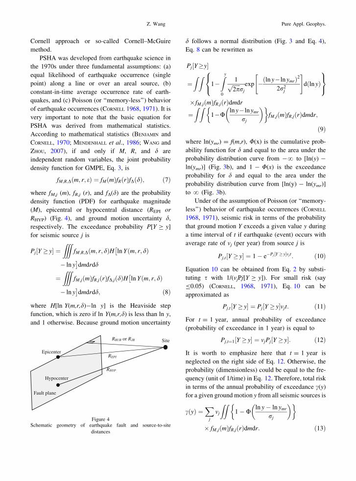
where fM,j (m), fR,j (r), and fD(d) are the probability

density function (PDF) for earthquake magnitude

(M), epicentral or hypocentral distance (REPI or

RHYP) (Fig. 4), and ground motion uncertainty d,

respectively. The exceedance probability P[Y C y]

for seismic source j is

Pj Y � y½ � ¼ZZZ

fM;R;Dðm; r; dÞH�ln Y m; r; dð Þ

� ln y�dmdrdd

¼ZZZ

fM;jðmÞfR;jðrÞfD;jðdÞH�ln Y m; r; dð Þ

� ln y�dmdrdd; ð8Þ

where H[ln Y(m,r,d)-ln y] is the Heaviside step

function, which is zero if ln Y(m,r,d) is less than ln y,

and 1 otherwise. Because ground motion uncertainty

d follows a normal distribution (Fig. 3 and Eq. 4),

Eq. 8 can be rewritten as

Pj Y�y½ �

¼Z Z

1�Zy

0

1ffiffiffiffiffiffi2pp

rj

exp � ln y� ln ymrð Þ2

2r2j

" #dðln yÞ

8<:

9=;

� fM;jðmÞfR;jðrÞdmdr

¼Z Z

1�Uln y� ln ymr

rj

� �� fM;jðmÞfR;jðrÞdmdr;

ð9Þ

where ln(ymr) = f(m,r), U(x) is the cumulative prob-

ability function for d and equal to the area under the

probability distribution curve from -? to [ln(y) -

ln(ymr)] (Fig. 3b), and 1 - U(x) is the exceedance

probability for d and equal to the area under the

probability distribution curve from [ln(y) - ln(ymr)]

to ? (Fig. 3b).

Under of the assumption of Poisson (or ‘‘memory-

less’’) behavior of earthquake occurrences (CORNELL

1968, 1971), seismic risk in terms of the probability

that ground motion Y exceeds a given value y during

a time interval of t if earthquake (event) occurs with

average rate of vj (per year) from source j is

Pj;t Y � y½ � ¼ 1� e�Pj Y � y½ �vjt: ð10Þ

Equation 10 can be obtained from Eq. 2 by substi-

tuting s with 1/(vjPj[Y C y]). For small risk (say

B0.05) (CORNELL, 1968, 1971), Eq. 10 can be

approximated as

Pj;t Y � y½ � ¼ Pj Y � y½ �vjt: ð11Þ

For t = 1 year, annual probability of exceedance

(probability of exceedance in 1 year) is equal to

Pj;t¼1 Y � y½ � ¼ vjPj Y � y½ �: ð12Þ

It is worth to emphasize here that t = 1 year is

neglected on the right side of Eq. 12. Otherwise, the

probability (dimensionless) could be equal to the fre-

quency (unit of 1/time) in Eq. 12. Therefore, total risk

in terms of the annual probability of exceedance c(y)

for a given ground motion y from all seismic sources is

cðyÞ ¼X

j

vj

ZZ1� U

ln y� ln ymr

rj

� ��

� fM;jðmÞfR;jðrÞdmdr: ð13Þ

Epicenter

RHYP

Fault plane

Hypocenter

REPI

RRUB or RJB Site

Figure 4Schematic geometry of earthquake fault and source-to-site

distances


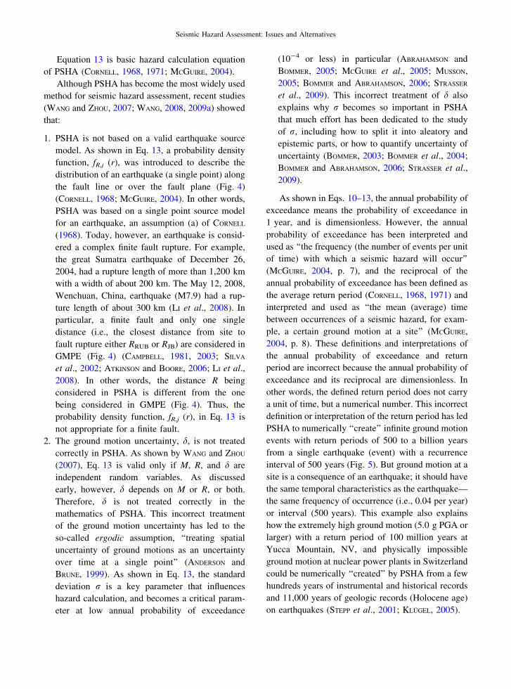
Equation 13 is basic hazard calculation equation

of PSHA (CORNELL, 1968, 1971; MCGUIRE, 2004).

Although PSHA has become the most widely used

method for seismic hazard assessment, recent studies

(WANG and ZHOU, 2007; WANG, 2008, 2009a) showed

that:

1. PSHA is not based on a valid earthquake source

model. As shown in Eq. 13, a probability density

function, fR,j (r), was introduced to describe the

distribution of an earthquake (a single point) along

the fault line or over the fault plane (Fig. 4)

(CORNELL, 1968; MCGUIRE, 2004). In other words,

PSHA was based on a single point source model

for an earthquake, an assumption (a) of CORNELL

(1968). Today, however, an earthquake is consid-

ered a complex finite fault rupture. For example,

the great Sumatra earthquake of December 26,

2004, had a rupture length of more than 1,200 km

with a width of about 200 km. The May 12, 2008,

Wenchuan, China, earthquake (M7.9) had a rup-

ture length of about 300 km (LI et al., 2008). In

particular, a finite fault and only one single

distance (i.e., the closest distance from site to

fault rupture either RRUB or RJB) are considered in

GMPE (Fig. 4) (CAMPBELL, 1981, 2003; SILVA

et al., 2002; ATKINSON and BOORE, 2006; LI et al.,

2008). In other words, the distance R being

considered in PSHA is different from the one

being considered in GMPE (Fig. 4). Thus, the

probability density function, fR,j (r), in Eq. 13 is

not appropriate for a finite fault.

2. The ground motion uncertainty, d, is not treated

correctly in PSHA. As shown by WANG and ZHOU

(2007), Eq. 13 is valid only if M, R, and d are

independent random variables. As discussed

early, however, d depends on M or R, or both.

Therefore, d is not treated correctly in the

mathematics of PSHA. This incorrect treatment

of the ground motion uncertainty has led to the

so-called ergodic assumption, ‘‘treating spatial

uncertainty of ground motions as an uncertainty

over time at a single point’’ (ANDERSON and

BRUNE, 1999). As shown in Eq. 13, the standard

deviation r is a key parameter that influences

hazard calculation, and becomes a critical param-

eter at low annual probability of exceedance

(10-4 or less) in particular (ABRAHAMSON and

BOMMER, 2005; MCGUIRE et al., 2005; MUSSON,

2005; BOMMER and ABRAHAMSON, 2006; STRASSER

et al., 2009). This incorrect treatment of d also

explains why r becomes so important in PSHA

that much effort has been dedicated to the study

of r, including how to split it into aleatory and

epistemic parts, or how to quantify uncertainty of

uncertainty (BOMMER, 2003; BOMMER et al., 2004;

BOMMER and ABRAHAMSON, 2006; STRASSER et al.,

2009).

As shown in Eqs. 10–13, the annual probability of

exceedance means the probability of exceedance in

1 year, and is dimensionless. However, the annual

probability of exceedance has been interpreted and

used as ‘‘the frequency (the number of events per unit

of time) with which a seismic hazard will occur’’

(MCGUIRE, 2004, p. 7), and the reciprocal of the

annual probability of exceedance has been defined as

the average return period (CORNELL, 1968, 1971) and

interpreted and used as ‘‘the mean (average) time

between occurrences of a seismic hazard, for exam-

ple, a certain ground motion at a site’’ (MCGUIRE,

2004, p. 8). These definitions and interpretations of

the annual probability of exceedance and return

period are incorrect because the annual probability of

exceedance and its reciprocal are dimensionless. In

other words, the defined return period does not carry

a unit of time, but a numerical number. This incorrect

definition or interpretation of the return period has led

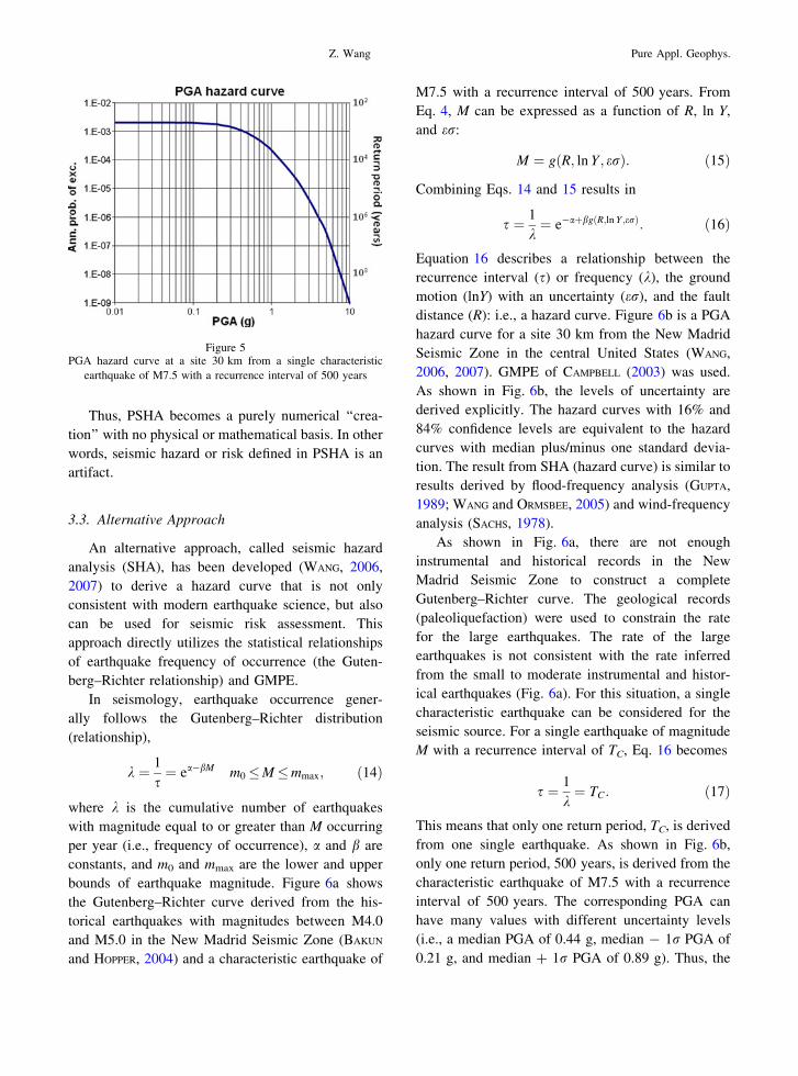
PSHA to numerically ‘‘create’’ infinite ground motion

events with return periods of 500 to a billion years

from a single earthquake (event) with a recurrence

interval of 500 years (Fig. 5). But ground motion at a

site is a consequence of an earthquake; it should have

the same temporal characteristics as the earthquake—

the same frequency of occurrence (i.e., 0.04 per year)

or interval (500 years). This example also explains

how the extremely high ground motion (5.0 g PGA or

larger) with a return period of 100 million years at

Yucca Mountain, NV, and physically impossible

ground motion at nuclear power plants in Switzerland

could be numerically ‘‘created’’ by PSHA from a few

hundreds years of instrumental and historical records

and 11,000 years of geologic records (Holocene age)

on earthquakes (STEPP et al., 2001; KLUGEL, 2005).


Thus, PSHA becomes a purely numerical ‘‘crea-

tion’’ with no physical or mathematical basis. In other

words, seismic hazard or risk defined in PSHA is an

artifact.

3.3. Alternative Approach

An alternative approach, called seismic hazard

analysis (SHA), has been developed (WANG, 2006,

2007) to derive a hazard curve that is not only

consistent with modern earthquake science, but also

can be used for seismic risk assessment. This

approach directly utilizes the statistical relationships

of earthquake frequency of occurrence (the Guten-

berg–Richter relationship) and GMPE.

In seismology, earthquake occurrence gener-

ally follows the Gutenberg–Richter distribution

(relationship),

k ¼ 1

s¼ ea�bM m0�M�mmax; ð14Þ

where k is the cumulative number of earthquakes

with magnitude equal to or greater than M occurring

per year (i.e., frequency of occurrence), a and b are

constants, and m0 and mmax are the lower and upper

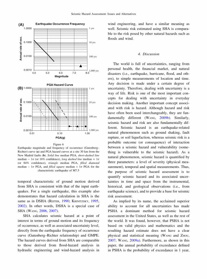
bounds of earthquake magnitude. Figure 6a shows

the Gutenberg–Richter curve derived from the his-

torical earthquakes with magnitudes between M4.0

and M5.0 in the New Madrid Seismic Zone (BAKUN

and HOPPER, 2004) and a characteristic earthquake of

M7.5 with a recurrence interval of 500 years. From

Eq. 4, M can be expressed as a function of R, ln Y,

and er:

M ¼ g R; ln Y ; erð Þ: ð15Þ

Combining Eqs. 14 and 15 results in

s ¼ 1

k¼ e�aþbg R;ln Y ;erð Þ: ð16Þ

Equation 16 describes a relationship between the

recurrence interval (s) or frequency (k), the ground

motion (lnY) with an uncertainty (er), and the fault

distance (R): i.e., a hazard curve. Figure 6b is a PGA

hazard curve for a site 30 km from the New Madrid

Seismic Zone in the central United States (WANG,

2006, 2007). GMPE of CAMPBELL (2003) was used.

As shown in Fig. 6b, the levels of uncertainty are

derived explicitly. The hazard curves with 16% and

84% confidence levels are equivalent to the hazard

curves with median plus/minus one standard devia-

tion. The result from SHA (hazard curve) is similar to

results derived by flood-frequency analysis (GUPTA,

1989; WANG and ORMSBEE, 2005) and wind-frequency

analysis (SACHS, 1978).

As shown in Fig. 6a, there are not enough

instrumental and historical records in the New

Madrid Seismic Zone to construct a complete

Gutenberg–Richter curve. The geological records

(paleoliquefaction) were used to constrain the rate

for the large earthquakes. The rate of the large

earthquakes is not consistent with the rate inferred

from the small to moderate instrumental and histor-

ical earthquakes (Fig. 6a). For this situation, a single

characteristic earthquake can be considered for the

seismic source. For a single earthquake of magnitude

M with a recurrence interval of TC, Eq. 16 becomes

s ¼ 1

k¼ TC: ð17Þ

This means that only one return period, TC, is derived

from one single earthquake. As shown in Fig. 6b,

only one return period, 500 years, is derived from the

characteristic earthquake of M7.5 with a recurrence

interval of 500 years. The corresponding PGA can

have many values with different uncertainty levels

(i.e., a median PGA of 0.44 g, median - 1r PGA of

0.21 g, and median ? 1r PGA of 0.89 g). Thus, the

Figure 5PGA hazard curve at a site 30 km from a single characteristic

earthquake of M7.5 with a recurrence interval of 500 years


temporal characteristic of ground motion derived

from SHA is consistent with that of the input earth-

quakes. For a single earthquake, this example also

demonstrates that hazard calculation in SHA is the

same as in DSHA (REITER, 1990; KRINITZSKY, 1995,

2002). In other words, DSHA is a special case of

SHA (WANG, 2006, 2007).

SHA calculates seismic hazard at a point of

interest in terms of ground motion and its frequency

of occurrence, as well as associated uncertainty level,

directly from the earthquake frequency of occurrence

curve (Gutenberg–Richter relationship) and GMPE.

The hazard curves derived from SHA are comparable

to those derived from flood-hazard analysis in

hydraulic engineering and wind-hazard analysis in

wind engineering, and have a similar meaning as

well. Seismic risk estimated using SHA is compara-

ble to the risk posed by other natural hazards such as

floods and wind.

4. Discussion

The world is full of uncertainties, ranging from

personal health, the financial market, and natural

disasters (i.e., earthquake, hurricane, flood, and oth-

ers), to simple measurements of location and time.

Any decision is made under a certain degree of

uncertainty. Therefore, dealing with uncertainty is a

way of life. Risk is one of the most important con-

cepts for dealing with uncertainty in everyday

decision making. Another important concept associ-

ated with risk is hazard. Although hazard and risk

have often been used interchangeably, they are fun-

damentally different (WANG, 2009b). Similarly,

seismic hazard and risk are also fundamentally dif-

ferent. Seismic hazard is an earthquake-related

natural phenomenon such as ground shaking, fault

rupture, or soil liquefaction, whereas seismic risk is a

probable outcome (or consequence) of interaction

between a seismic hazard and vulnerability (some-

thing is vulnerable to the seismic hazard). As a

natural phenomenon, seismic hazard is quantified by

three parameters: a level of severity (physical mea-

surement), temporal and spatial measurements. Thus,

the purpose of seismic hazard assessment is to

quantify seismic hazard and its associated uncer-

tainties in time and space from the instrumental,

historical, and geological observations (i.e., from

earthquake science), and to provide a base for seismic

risk assessment.

As implied by its name, the acclaimed superior

ability to account for all uncertainties has made

PSHA a dominant method for seismic hazard

assessment in the United States, as well as the rest of

the world. It was found, however, that PSHA is not

based on valid physics and mathematics and the

resulting hazard estimate does not have a clear

physical and statistical meaning (WANG and ZHOU,

2007; WANG, 2009a). Furthermore, as shown in this

paper, the annual probability of exceedance defined

in PSHA is the probability of exceedance in 1 year,

Earthquake Occurrence Frequency

0.0010

0.0100

0.1000

1.0000

4.0 5.0 6.0 7.0 8.0Magnitude

Ann

ual r

ate

of e

xc.

PGA Hazard Curve

0.0010

0.0100

0.1000

1.0000

0.01 0.10 1.00

PGA(g)

An

nual

rat

e o

f ex

c.

1,000 yrs

1 yrs

100 yrs

1,000 yrs

100 yrs

10 yrs

10 yrs

(B)

(A)1 yrs

Figure 6Earthquake magnitude and frequency of occurrence (Gutenberg–

Richter) curve (a) and PGA hazard curves at a site 30 km from the

New Madrid faults (b). Solid line median PGA, short-dashed line

median - 1r (or 16% confidence), long dashed line median ? 1r(or 84% confidence), triangle median PGA, filled diamond

median - 1r PGA, and filled square median ? 1r PGA for the

characteristic earthquake of M7.5


and is dimensionless. The return period, defined as

the reciprocal of the annual probability of exceedance

(CORNELL, 1968, 1971), is also dimensionless. How-

ever, the annual probability of exceedance has been

interpreted and used as ‘‘the frequency (the number of

events per unit of time) with which a seismic hazard

will occur’’ (MCGUIRE, 2004, p. 7), and the return

period has been interpreted and used as ‘‘the mean

(average) time between occurrences of a seismic

hazard, for example, a certain ground motion at a

site’’ (MCGUIRE, 2004, p. 8). Therefore, PSHA is a

pure numerical ‘‘creation’’ or model without physical

and mathematical bases.

The results derived from PSHA are all artifact and

difficult to understand and use. This can explain why

the most important effort in current PSHA practice is

on how to count, re-count, and split uncertainties, but

not on earthquake physics and statistics (SSHAC,

1997; ABRAHAMSON and BOMMER, 2005; MCGUIRE

et al., 2005; MUSSON, 2005; BOMMER and ABRAHAM-

SON, 2006; STRASSER et al., 2009). In other words,

practice of PSHA becomes a personal belief, but not a

science. If they are purely academic, the problems

with PSHA may not be of concern. However, the

problems with PSHA have far reaching implications

for society; from seismic design of buildings, bridges,

nuclear power plants, to earthquake insurance pre-

miums. For example, according to a PSHA study by

STEPP et al. (2001), which is one of the most com-

prehensive PSHA studies in the world, a PGA of 10 g

might have to be considered for engineering design of

nuclear repository facility at Yucca Mountain in

Nevada. The use of the national seismic hazard maps

which were produced from PSHA (FRANKEL et al.

1996, 2002; PETERSEN et al., 2008) could lead to a

similar or even higher design ground motion in

Memphis, TN, and Paducah, KY (STEIN et al., 2003;

WANG et al., 2003). On the other hand, the Chinese

national seismic design ground motion (PRCNS,

2001), which was also derived from PSHA, was

found to be too low in the Wenchuan, China earth-

quake area (XIE et al., 2009). This is one of the

reasons why the losses from the Wenchuan earth-

quake were so high.

Although the biggest criticism of DSHA is that

‘‘it (DSHA) does not take into account the inherent

uncertainty in seismic hazard estimation’’ (REITER,

1990, p. 225), the truth is that DSHA accounts for

all the inherent uncertainty explicitly. For example,

the maximum credible earthquake (MCE) ground

motion is usually taken at a mean ? 1 standard

deviation (i.e., 84th percentile) in the scatter of

recorded earthquake ground motions (KRINITZSKY,

1995, 2002; MUALCHIN, 1996; KLUGEL et al., 2006).

The weakness of DSHA is that ‘‘frequency of

occurrence is not explicitly taken into account’’

(REITER, 1990, p. 225). In other words, the temporal

characteristic of ground motion (i.e., occurrence

interval or frequency and its associated uncertainty)

is not addressed or often neglected in DSHA. The

temporal characteristic of ground motion is an

integral part of seismic hazard and must be con-

sidered in engineering design and other policy

consideration. One of the improvements for DSHA

is to address the temporal characteristics. Actually,

as pointed out by WANG et al. (2004), a determin-

istic earthquake can always be associated with a

recurrence interval and its uncertainty.

SHA directly utilizes earthquake statistical rela-

tionships, earthquake frequency of occurrence

(Gutenburg-Richter relationship), and GMPE to

predict ground motion at a point of interest. The

hazard curves derived from SHA are comparable to

those derived from flood-hazard analysis in hydrau-

lic engineering and wind-hazard analysis in wind

engineering, and have a similar meaning. Seismic

risk estimated using SHA is comparable to the risk

posed by other natural hazards such as hurricanes,

winter storms, and volcanic eruptions. As discussed

earlier, SHA depends on the earthquake frequency of

occurrence relationship. As pointed out by KRINITZ-

SKY (KRINITZSKY, 1993a, b), there may not be enough

earthquake records to construct a reliable frequency

relationship for a specific seismic source zone, par-

ticularly for a fault zone. Therefore, SHA may not

be applicable to areas where earthquake records are

scarce or seismicity is low. For the areas with

limited earthquake records, a single or a few earth-

quakes (i.e., maximum credible earthquake,

maximum considered earthquake, or maximum

design earthquake) are often considered for engi-

neering design and other policies. Under this

situation, SHA and DSHA are the same. Therefore,

DSHA is a special case of SHA.


5. Conclusion

Seismic hazard assessment is an effort to quantify

seismic hazard and its associated uncertainty by earth

scientists. As for any natural or man-made events,

such as hurricanes and terrorist attacks, an earthquake

has a unique position in time and space. In other

words, how to quantify the temporal and spatial

characteristics of seismic hazard is the core of a

seismic hazard assessment. Although PSHA has been

proclaimed as the best method and is used widely for

seismic hazard assessment, neither the physical

model nor the mathematical formulation is valid. In

other words, PSHA is a purely numerical ‘‘creation’’

with no physical or mathematical basis. Thus, PSHA

should not be used for seismic hazard assessment,

and use of PSHA could lead to either unsafe or overly

conservative engineering design, with dire conse-

quences for society.

On the other hand, even though DSHA has been

labeled as an unreliable approach, it actually has been

more widely used for seismic hazard assessment. In

California, the design ground motion for bridges and

buildings was determined from DSHA, not PSHA

(MUALCHIN, 1996; KIRCHER et al., 2008). DSHA has

clear earthquake physics and statistics. The biggest

criticism of DSHA, particularly by PSHA propo-

nents, has been its inability to account for

uncertainty. This is not true, however. DSHA

accounts for all the inherent uncertainty in an explicit

and appropriate way. The biggest drawback of DSHA

is that the temporal characteristics (i.e., the recur-

rence interval or frequency of ground motion) are

often time neglected. This is one of the areas that

need to be addressed or improved in DSHA.

As an alternative, SHA utilizes all aspects of

earthquake science and statistics to provide a seismic

hazard estimate that can be readily used for seismic

risk assessment and other applications. The limitation

of SHA is that there may not be enough earthquake

records to construct a reliable earthquake frequency

of occurrence relationship in areas where earthquake

records are scarce or seismicity is low. SHA and

DSHA are the same for areas where only a single or a

few earthquakes (i.e., maximum credible earthquake,

maximum considered earthquake, or maximum

design earthquake) are considered.

Acknowledgments

I thank Meg Smath of the Kentucky Geological

Survey for editorial help. I appreciate comments and

suggestions from Kelin Wang. I also appreciate the

comments and suggestions from Kojiro Irikura and

two anonymous reviewers, which help to improve the

manuscript greatly.

REFERENCES

ABRAHAMSON, N. A. and BOMMER, J. J. (2005), Probability and

uncertainty in seismic hazard analysis, Earthq Spectra 21, 603–

607

ABRAHAMSON, N. A. and SILVA, W. J. (1997), Empirical response

spectral attenuation relations for shallow crustal earthquake,

Seism Res Lett 68, 94–108

ABRAHAMSON, N. A. and SILVA, W. J. (2008), Summary of the

Abrahamson and Silva NGA ground motion relations, Earthq

Spectra 24, 67–97

ANDERSON, G. A. and BRUNE, J. N. (1999), Probabilistic seismic

hazard analysis without the ergodic assumption, Seism Res Lett

70, 19–28

ATKINSON, G. M. and BOORE, D. M. (2006), Earthquake ground-

motion prediction equations for eastern North America, Bull

Seismol Soc Am 96, 2181–2205

BAKUN, W. H. and HOPPER, M. G. (2004), Historical seismic activity

in the central United States, Seism Res Lett 75, 564–574

BAZZURRO, P. and CORNELL, C. A. (1999), Disaggregation of seismic

hazard, Bull Seismol Soc Am 89, 501–520

BENJAMIN, J. R., CORNELL, C. A. (1970), Probability, statistics, and

decision for civil engineers, New York, McGraw-Hill Book

Company, 684 p

BOMMER, J. J. (2003), Uncertainty about the uncertainty in seismic

hazard analysis, Eng Geol 70, 165–168

BOMMER, J. J. and ABRAHAMSON, N. A. (2006), Why do modern

probabilistic seismic-hazard analyses often lead to increased

hazard estimates? Bull Seismol Soc Am 96, 1976–1977

BOMMER, J. J., ABRAHAMSON, N. A., STRASSER, F. O., PECKER, A.,

BARD, P.-Y., BUNGUM, H., COTTON, F., FAH, D., SABETTA, F.,

SCHERBAUM, F., and STUDER, J. (2004), The challenge of defining

upper bounds on earthquake ground motions, Seism Res Lett 75,

82–95

BOORE, D. M., JOYNER, W. B., and FUMAL, T. E. (1997), Equations

for estimating horizontal response spectra and peak acceleration

from western North American earthquakes: A summary of recent

work, Seism Res Lett 68,128–153

BUILDING SEISMIC SAFETY COUNCIL (BSSC). (1998), NEHRP rec-

ommended provisions for seismic regulations for new buildings

[1997 ed.], Federal Emergency Management Agency, FEMA,

302, 337 pp

CAMPBELL, K. W. (1981), Near-source attenuation of peak hori-

zontal acceleration, Bull Seismol Soc Am 71, 2039–2070

CAMPBELL, K. W. (2003), Prediction of strong ground motion using

the hybrid empirical method and its use in the development of

ground-motion (attenuation) relations in eastern North America,

Bull Seismol Soc Am 93, 1012–1033


CORNELL, C. A. (1968), Engineering seismic risk analysis, Bull

Seismol Soc Am 58, 1583–1606

CORNELL, C. A. (1971), Probabilistic analysis of damage to struc-

tures under seismic loads. In Dynamic Waves in Civil

Engineering (eds. Howells, D. A., Haigh, I. P., and Taylor, C.),

Proceedings of a Conference Organized by the Society for

Earthquake and Civil Engineering Dynamics (John Wiley, New

York)

FRANKEL, A., MUELLER, C., BARNHARD, T., LEYENDECKER, E.V.,

WESSON, R. L., HANSON, S., KLEIN, F. W., PERKINS, D. E., DICK-

MAN, N., and HOPPER, M. (2000), USGS national seismic hazard

maps, Earthq Spectra 16, 1–19

FRANKEL, A., PETERSEN, M., MUELLER, C., HALLER, K., WHEELER, R.,

LEYENDECKER, E., WESSON, R., HARMSEN, S., CRAMER, C., PERKINS,

D., and RUKSTALES, K. (2002), Documentation for the 2002

update of the national seismic hazard maps, U.S. Geological

Survey Open-File Report 02-420, 33 pp

FRANKEL, A., MUELLER, C., BARNHARD, T., PERKINS, D., LEYENDEC-

KER, E., DICKMAN, N., HANSON, S., and HOPPER, M. (1996),

National seismic hazard maps: Documentation June 1996, U.S.

Geological Survey Open-File Report 96-532, 110 pp

GUPTA, R. S., Hydrology and Hydraulic Systems (Prentice Hall,

Englewood Cliffs, N.J., 1989), 739 pp

INTERNATIONAL CODE COUNCIL (ICC). (2006), International Building

Bode (International Code Council Inc.)

KIRCHER, C. A., LUCO, N., and WHITTAKER, A. (2008), Summary of

SDPRG proposal for changes to the 2009 NEHRP provisions,

Building Seismic Safety Council Seismic Design Procedures

Reassessment Group (SDPRG) workshop, September 10, 2008,

Burlingame, California

KIRCHER, C. A., SELIGSON, H. A., BOUABID, J., and MORROW, G. C.

(2006), When the Big One strikes again—Estimated losses due to

a repeat of the 1906 San Francisco earthquake. In Proceedings of

the 8th National Conference on Earthquake Engineering, April

18–22, 2006, San Francisco, CA

KLUGEL, J.-U. (2005), Problems in the application of the SSHAC

probability method or assessing earthquake hazards at Swiss

nuclear power plants, Eng Geol 78, 285–307

KLUGEL, J.-U., MUALCHIN, L., and PANZA, G. F. (2006), A scenario-

based procedure for seismic risk analysis, Eng Geol 88, 1–22

KRINITZSKY, E. L. (1993a), Earthquake probability in engineering—

Part 1: The use and misuse of expert opinion, Eng Geol 33, 257–

288

KRINITZSKY, E. L. (1993b), Earthquake probability in engineering—

Part 2: Earthquake recurrence and limitations of Gutenburg-

Richter b-values for the engineering of critical structures, Eng

Geol 36, 1–52

KRINITZSKY, E. L. (1995), Deterministic versus probabilistic seismic

hazard analysis for critical structures, Eng Geol 40, 1–7

KRINITZSKY, E. L. (2002), How to obtain earthquake ground

motions for engineering design, Eng Geol 65, 1–16

LEYENDECKER, E. V., HUNT, R. J., FRANKEL, A. D., and RUKSTALES,

K. S. (2000), Development of maximum considered earthquake

ground motion maps, Earthq Spectra 16, 21–40

LI, X., ZHOU, Z., HUANG, M., WEN, R., YU, H., LU, D., ZHOU, Y., and

CUI, J. (2008), Preliminary analysis of strong-motion recordings

from the magnitude 8.0 Wenchuan, China, earthquake of 12 May

2008, Seism Res Lett 79, 844–854

LUCO, N. (2008), Risk-Targeted Ground Motions: Building Seismic

Safety Council Seismic Design Procedures Reassessment Group

(SDPRG) workshop, September 10, 2008, Burlingame, CA

MALHOTRA, P. K. (2008), Seismic design loads from site-specific

and aggregate hazard analyses, Bull Seismol Soc Am 98, 1849–

1862

MCGUIRE, R. K. (2004), Seismic hazard and risk analysis, Earth-

quake Engineering Research Institute, MNO-10, 240 pp

MCGUIRE, R. K., CORNELL, C. A., and TORO, G. R. (2005), The case

for using mean seismic hazard, Earthq Spectra 21, 879–886

MENDENHALL, W., SCHEAFFER, R. L., WACKERLY, D. D. (1986),

Mathematical statistics with applications, Boston, Duxbury

Press, 750 p

MILNE, W. G., DAVENPORT, A. G. (1969), Distribution of earthquake

risk in Canada, Bull Seismol Soc Am 59, 729–754

MUALCHIN, L., 1996, Development of the Caltrans deterministic

fault and earthquake hazard map of California, Eng Geol 42,

217–222

MUSSON, R. M. W. (2005), Against fractiles, Earthq Spectra 21,

887–891

PETERSEN, M. D., FRANKEL, A. D., HARMSEN, S. C., MUELLER, C. S.,

HALLER, K. M., WHEELER, R. L., WESSON, R. L., ZENG, Y., BOYD,

O. S., PERKINS, D. M., LUCO, N., FIELD, E. H., WILLS, C. J., and

RUKSTALES, K. S. (2008), Documentation for the 2008 update of

the United States national seismic hazard maps, U.S. Geological

Survey Open-File Report 08-1128, 60 pp

PEOPLE’S REPUBLIC OF CHINA NATIONAL STANDARD (PRCNS). (2001),

Seismic ground motion parameter zonation map of China, GB

18306-2001, China Standard Press

REITER, L., Earthquake Hazard Analysis (Columbia University

Press, New York, 1990), 254 pp

SACHS, P., Wind Forces In Engineering, 2nd edn. (Pergamon Press

Inc., Elmsford, N.Y., 1978), 400 pp

SENIOR SEISMIC HAZARD ANALYSIS COMMITTEE (SSHAC). (1997),

Recommendations for probabilistic seismic hazard analysis:

Guidance on uncertainty and use of experts, Lawrence Livermore

National Laboratory, NUREG/CR-6372, 81 pp

SILVA, W., GREGOR, N., and DARRAGH, R. (2002), Development of

regional hard rock attenuation relationships for central and

eastern North America, Pacific Engineering and Analysis, 311

Pomona Ave., El Cerrito, Calif., 94530, 57 pp

STEIN, S., TOMASELLO, J., and NEWMAN, A. (2003), Should Memphis

build for California’s earthquakes? EOS, Trans AGU 84, 177,

184–185

STEPP, J. C., WONG, I., WHITNEY, J., QUITTMEYER, R., ABRAHAMSON,

N., TORO, G., YOUNGS, R., COPPERSMITH, K., SAVY, J., SULLIVAN,

T., and YUCCA MOUNTAIN PSHA PROJECT MEMBERS. (2001),

Probabilistic seismic hazard analysis for ground motions and

fault displacements at Yucca Mountain, Nevada, Earthq Spectra

17, 113–151

STRASSER, F. O., ABRAHAMSON, N. A., and BOMMER, J. J. (2009),

Sigma: Issues, insights, and challenges, Seism Res Lett 80, 41–

56

U.S. GEOLOGICAL SURVEY. (2009), Important note on use of new

2008 USGS hazard maps: earthquake.usgs.gov/research/haz-

maps/products_data/2008/disclaimer.php. Accessed 9/2/2009

WANG, Z. (2006), Understanding seismic hazard and risk assess-

ments: An example in the New Madrid Seismic Zone of the

central United States. In Proceedings of the 8th National Con-

ference on Earthquake Engineering, April 18–22, 2006, San

Francisco, Calif., paper 416

WANG, Z. (2007), Seismic hazard and risk assessment in the

intraplate environment: The New Madrid Seismic Zone of the

central United States. In Continental Intraplate Earthquakes:


Science, Hazard, And Policy Issues (eds. Stein, S. and Mazzotti,

S.), Geological Society of America Special Paper 425, pp. 363–

373

WANG, Z. (2008), Understanding seismic hazard and risk: A gap

between engineers and seismologists. In 14th World Conference

on Earthquake Engineering, October 12–17, 2008, Beijing,

China, Paper S27-001, 11 pp

WANG, Z. (2009a), Comment on ‘‘Sigma: Issues, Insights, and

Challenges’’ by Fleur O. Strasser, Norman A. Abrahamson, and

Julian J. Bommer, Seismol Res Lett 80, 491–493

WANG, Z. (2009b), Seismic hazard vs. seismic risk, Seismol Res

Lett 80, 673–674

WANG, Z. and ORMSBEE, L. (2005), Comparison between probabi-

listic seismic hazard analysis and flood frequency analysis, EOS

Trans AGU 86, 45, 51–52

WANG, Z., WOOLERY, E. W., SHI, B., and KIEFER, J. D. (2003),

Communicating with uncertainty: A critical issue with probabi-

listic seismic hazard analysis, EOS Trans AGU 84, 501, 506, 508

WANG, Z., WOOLERY, E. W., SHI, B., and KIEFER, J. D. (2004), Reply

to Comment on ‘‘Communicating with uncertainty: A critical

issue with probabilistic seismic hazard analysis’’ by C.H. Cra-

mer, EOS Trans AGU 85, 283, 286

WANG, Z. and ZHOU, M. (2007), Comment on ‘‘Why do modern

probabilistic seismic-hazard analyses often lead to increased

hazard estimates?’’ by Julian J. Bommer and Norman A. Abra-

hamson, Bull Seismol Soc Am 97, 2212–2214

WORKING GROUP on CALIFORNIA EARTHQUAKE PROBABILITIES

(WGCEP). (2003), Earthquake probabilities in the San Fran-

cisco Bay Region: 2002–2031, U.S. Geological Survey Open-

File Report 03-214, 235 pp

XIE, F., WANG, Z., DU, Y., and ZHANG, X. (2009), Preliminary

observations of the faulting and damage pattern of M8.0

Wenchuan, China, earthquake, Prof Geol 46(4), 3–6

YOUNGS, R. R., ABRAHAMSON, N., MAKDISI, F. I., and SADIGH, K.

(1995), Magnitude-dependent variance of peak ground acceler-

ation, Bull Seismol Soc Am 85, 1161–1176

(Received March 26, 2009, revised December 16, 2009, accepted March 31, 2010)


Download - Seismic Hazard Assessment: Issues and AlternativesSeismic Hazard Assessment: Issues and Alternatives ZHENMING WANG 1 Abstract—Seismic hazard and risk are two very important concepts

Top Related