Download - Searching: Self Organizing Structures and Hashing CS 400/600 – Data Structures

Searching: Self Organizing Searching: Self Organizing Structures and HashingStructures and Hashing

CS 400/600 – Data StructuresCS 400/600 – Data Structures

Search and Hashing 2

SearchingSearching Records contain information and keys

• <k1, I1>, <k2, I2>, …, <kn, In>

Find all records with key value K May be successful or unsuccessful Range query: all records with key values

between Klow and Khigh


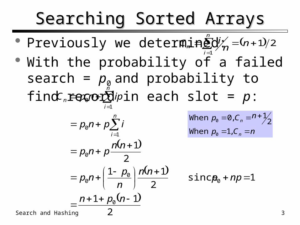
Searching Sorted ArraysSearching Sorted Arrays Previously we determined: With the probability of a failed search = p0 and

probability to find record in each slot = p:

n

in nn

iC1

21

2

11

1 since2

112

1

0

00

0

0

10

10

npn

nppnn

n

pnp

nnpnp

ipnp

ipnpC

n

i

n

in

nCp

nCp

n

n

,1When 2

1 ,0When

0

0


Self OrganizationSelf Organization 80/20 Rule – In many applications, 80% of the

accesses reference 20% of the records If we sorted the records by the frequency that

they will be accessed, then a linear search through the array can be efficient

Since we don’t know what the actual access pattern will be, we use heuristics to order the array


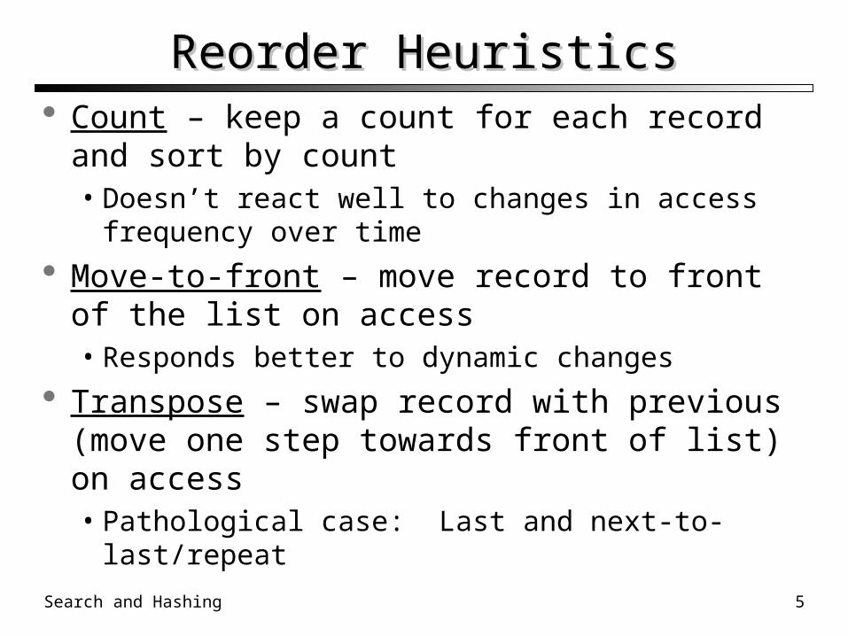
Reorder HeuristicsReorder Heuristics Count – keep a count for each record and sort

by count• Doesn’t react well to changes in access frequency

over time

Move-to-front – move record to front of the list on access• Responds better to dynamic changes

Transpose – swap record with previous (move one step towards front of list) on access• Pathological case: Last and next-to-last/repeat


Analysis of Self Organizing ListsAnalysis of Self Organizing Lists Slower search than search trees or sorted lists Fast insert Simple to implement Very efficient for small lists


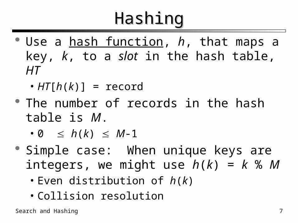
HashingHashing Use a hash function, h, that maps a key, k, to a

slot in the hash table, HT• HT[h(k)] = record

The number of records in the hash table is M.• 0 h(k) M-1

Simple case: When unique keys are integers, we might use h(k) = k % M• Even distribution of h(k)• Collision resolution


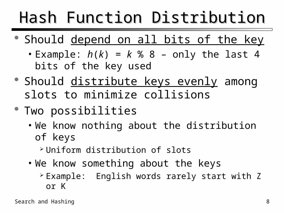
Hash Function DistributionHash Function Distribution Should depend on all bits of the key

• Example: h(k) = k % 8 – only the last 4 bits of the key used

Should distribute keys evenly among slots to minimize collisions

Two possibilities• We know nothing about the distribution of keys

Uniform distribution of slots

• We know something about the keys Example: English words rarely start with Z or K


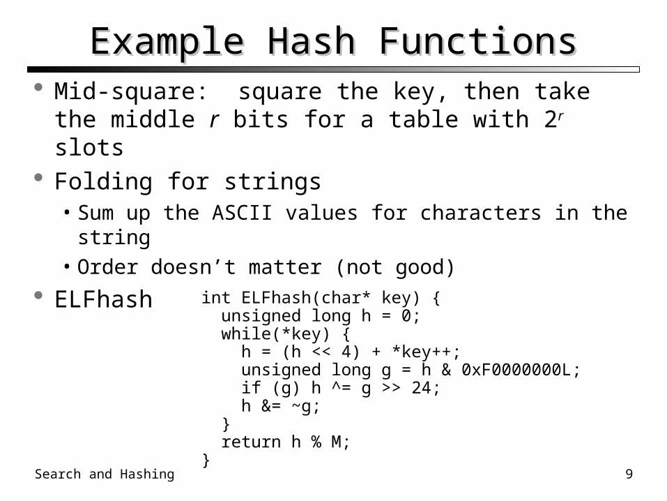
Example Hash FunctionsExample Hash Functions Mid-square: square the key, then take the

middle r bits for a table with 2r slots Folding for strings

• Sum up the ASCII values for characters in the string• Order doesn’t matter (not good)

ELFhash int ELFhash(char* key) { unsigned long h = 0; while(*key) { h = (h << 4) + *key++; unsigned long g = h & 0xF0000000L; if (g) h ^= g >> 24; h &= ~g; } return h % M;}


Open HashingOpen Hashing

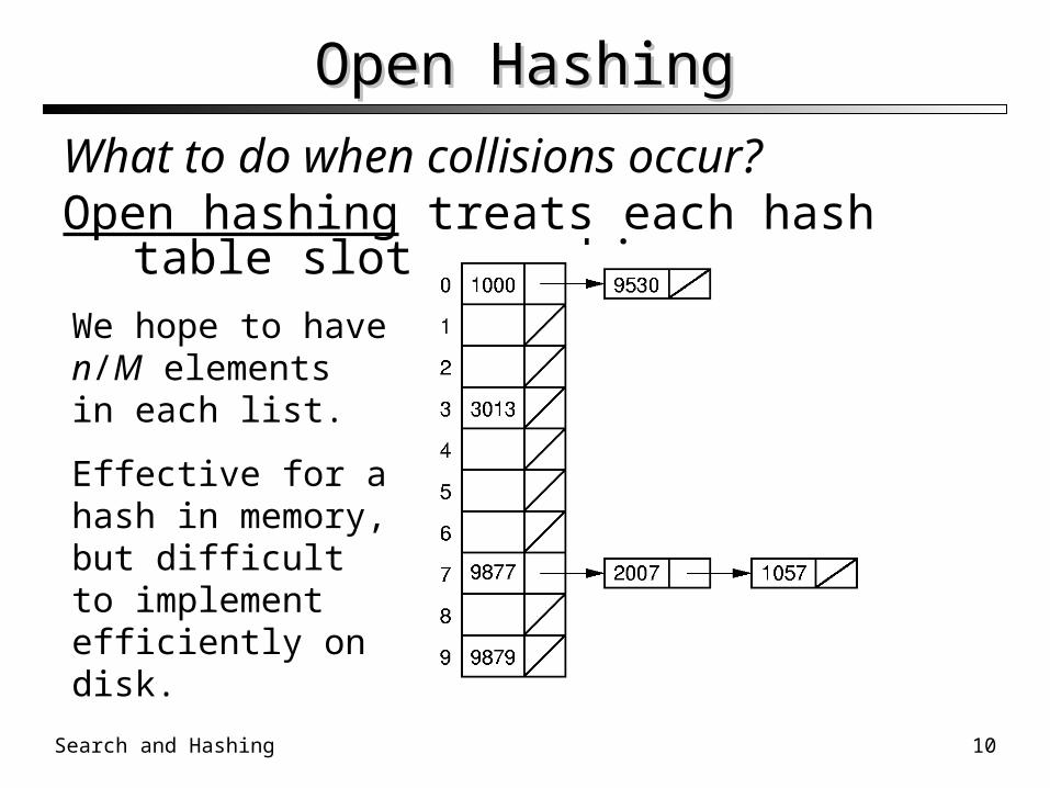
What to do when collisions occur?Open hashing treats each hash table slot as a bin.

We hope to have n/M elements in each list.

Effective for a hash in memory, but difficult to implement efficiently on disk.


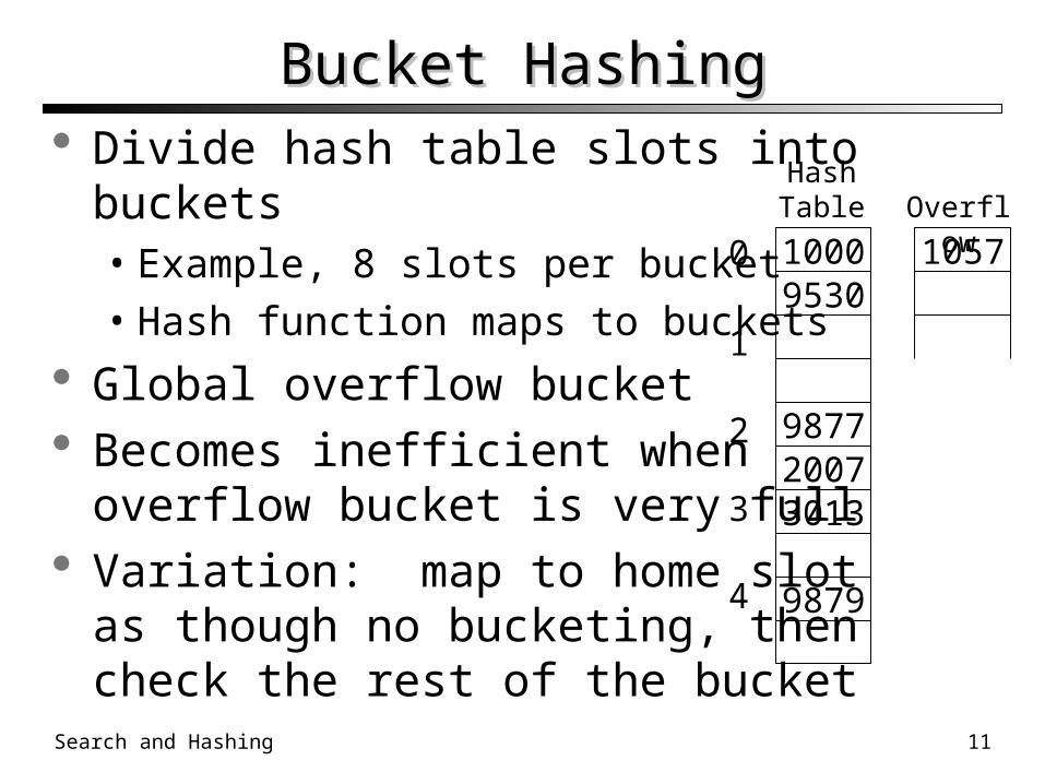
Bucket HashingBucket Hashing Divide hash table slots into buckets

• Example, 8 slots per bucket• Hash function maps to buckets

Global overflow bucket Becomes inefficient when

overflow bucket is very full Variation: map to home slot

as though no bucketing, thencheck the rest of the bucket

10009530

987720073013

9879

0

1

2

3

4

Hash Table

1057Overflow


Closed HashingClosed Hashing

Closed hashing stores all records directly in the hash table.• Bucket hashing is a type of closed hasing

Each record i has a home position h(ki).

If another record occupies i’s home position, then another slot must be found to store i.

The new slot is found by a collision resolution policy.

Search must follow the same policy to find records not in their home slots.


Collision ResolutionCollision Resolution

During insertion, the goal of collision resolution is to find a free slot in the table.

Probe sequence: The series of slots visited during insert/search by following a collision resolution policy.

Let 0 = h(K). Let (0, 1, …) be the series of slots making up the probe sequence.


InsertionInsertion

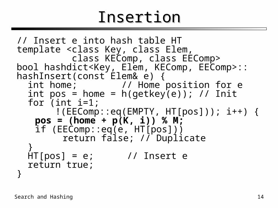
// Insert e into hash table HTtemplate <class Key, class Elem, class KEComp, class EEComp>bool hashdict<Key, Elem, KEComp, EEComp>::hashInsert(const Elem& e) { int home; // Home position for e int pos = home = h(getkey(e)); // Init for (int i=1; !(EEComp::eq(EMPTY, HT[pos])); i++)

{pos = (home + p(K, i)) % M;if (EEComp::eq(e, HT[pos]))

return false; // Duplicate } HT[pos] = e; // Insert e return true;}


SearchSearch

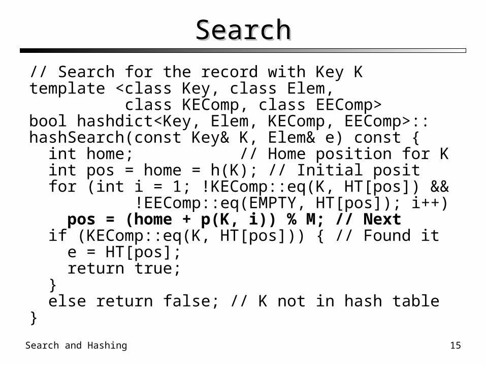
// Search for the record with Key Ktemplate <class Key, class Elem, class KEComp, class EEComp>bool hashdict<Key, Elem, KEComp, EEComp>::hashSearch(const Key& K, Elem& e) const { int home; // Home position for K int pos = home = h(K); // Initial posit for (int i = 1; !KEComp::eq(K, HT[pos]) && !EEComp::eq(EMPTY, HT[pos]); i++) pos = (home + p(K, i)) % M; // Next if (KEComp::eq(K, HT[pos])) { // Found it e = HT[pos]; return true; } else return false; // K not in hash table}


Probe FunctionProbe Function

Look carefully at the probe function p().pos = (home + p(getkey(e), i)) % M;

Each time p() is called, it generates a value to be added to the home position to generate the new slot to be examined.

p() is a function both of the element’s key value, and of the number of steps taken along the probe sequence.

• Not all probe functions use both parameters.


Linear ProbingLinear Probing

Use the following probe function:

p(K, i) = i;

Linear probing simply goes to the next slot in the table.

• Past bottom, wrap around to the top.

To avoid infinite loop, one slot in the table must always be empty.


Linear Probing ExampleLinear Probing Example

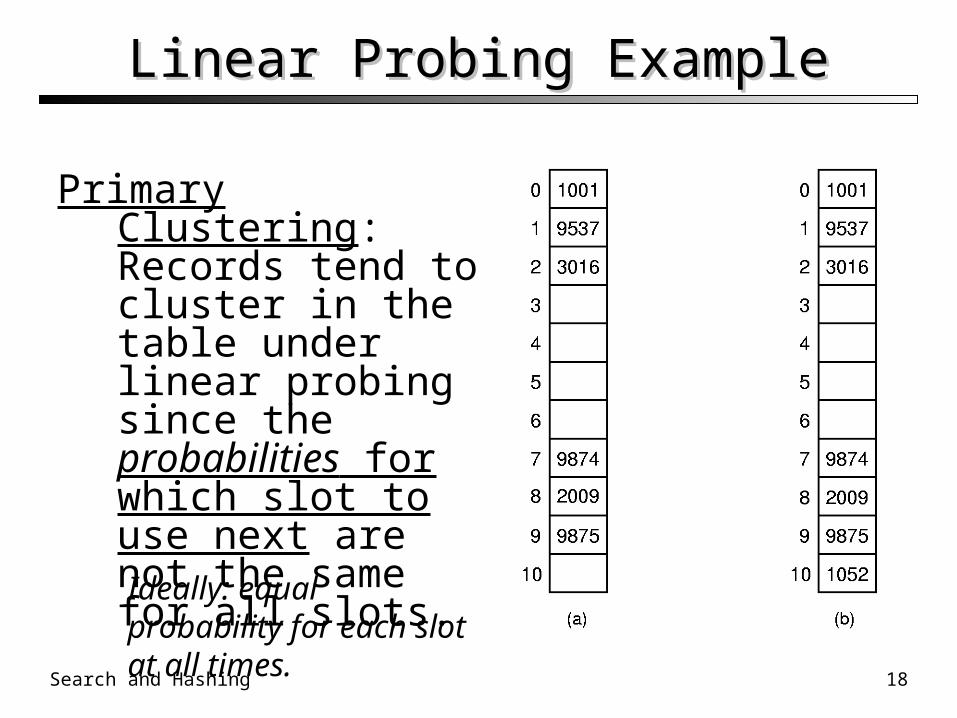
Primary Clustering: Records tend to cluster in the table under linear probing since the probabilities for which slot to use next are not the same for all slots.

Ideally: equal probability for each slot at all times.


Improved Linear ProbingImproved Linear Probing

Instead of going to the next slot, skip by some constant c.• Warning: Pick M and c carefully.• Example: c=2 and M=10 two hash tables!

The probe sequence SHOULD cycle through all slots of the table.

• Pick c to be relatively prime to M.

There is still some clustering• Ex: c=2, h(k1) = 3; h(k2) = 5.• Probe sequences for k1 and k2 are linked together.


Pseudo-random ProbingPseudo-random Probing Ideally, for any two keys, k1 and k2, the probe

sequences should diverge. An ideal probe function would select the next

value in the probe sequence at random.• Why can’t we do this?

Select a random permutation of the numbers from 1 to M1:

Perm = [r1, r2, r3, …, rM-1]

p(K, i) = Perm[i-1];


Pseudo-random probe examplePseudo-random probe example

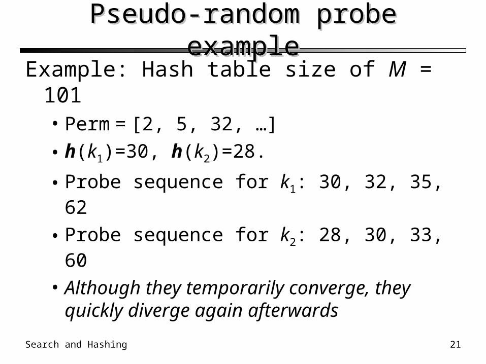
Example: Hash table size of M = 101• Perm = [2, 5, 32, …]

• h(k1)=30, h(k2)=28.

• Probe sequence for k1: 30, 32, 35, 62

• Probe sequence for k2: 28, 30, 33, 60

• Although they temporarily converge, they quickly diverge again afterwards


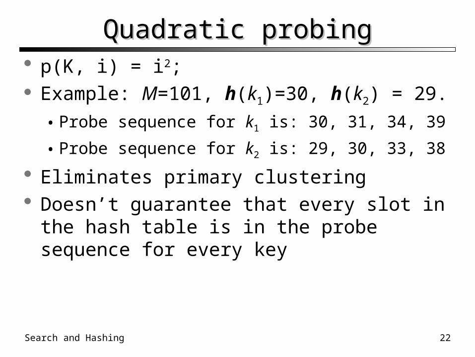
Quadratic probingQuadratic probing p(K, i) = i2; Example: M=101, h(k1)=30, h(k2) = 29.

• Probe sequence for k1 is: 30, 31, 34, 39

• Probe sequence for k2 is: 29, 30, 33, 38

Eliminates primary clustering Doesn’t guarantee that every slot in the hash

table is in the probe sequence for every key


Secondary ClusteringSecondary Clustering Pseudo-random probing eliminates primary

clustering. If two keys hash to the same slot, they follow

the same probe sequence. This is called secondary clustering.

To avoid secondary clustering, need probe sequence to be a function of the original key value, not just the home position.• None of the probe functions we have looked at use

K in any way!


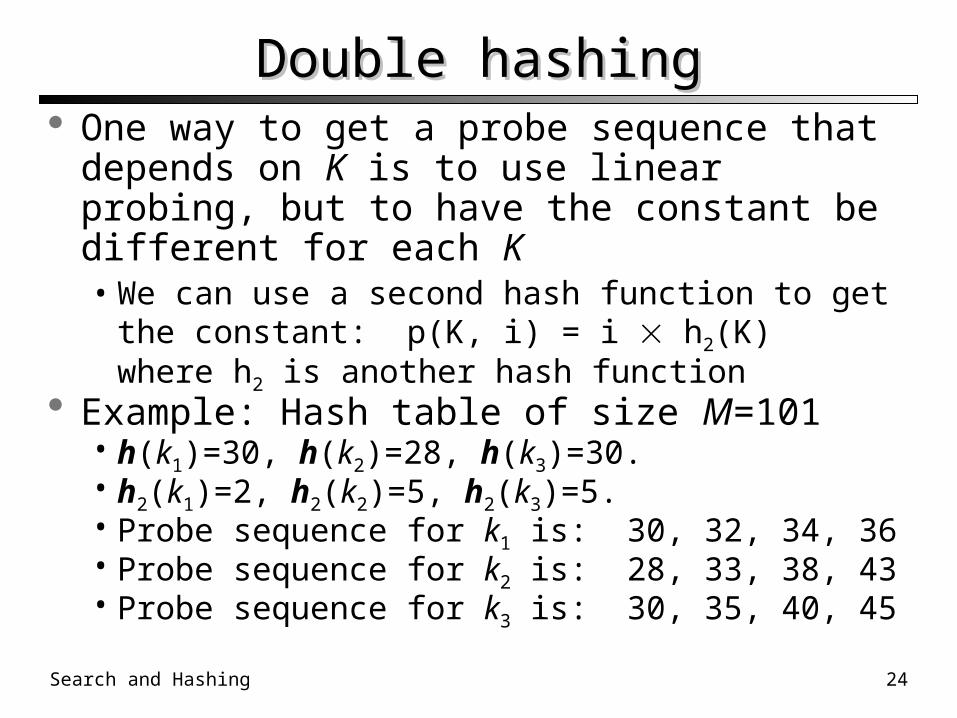
Double hashingDouble hashing One way to get a probe sequence that depends

on K is to use linear probing, but to have the constant be different for each K• We can use a second hash function to get the

constant: p(K, i) = i h2(K)where h2 is another hash function

Example: Hash table of size M=101• h(k1)=30, h(k2)=28, h(k3)=30.• h2(k1)=2, h2(k2)=5, h2(k3)=5.• Probe sequence for k1 is: 30, 32, 34, 36• Probe sequence for k2 is: 28, 33, 38, 43• Probe sequence for k3 is: 30, 35, 40, 45


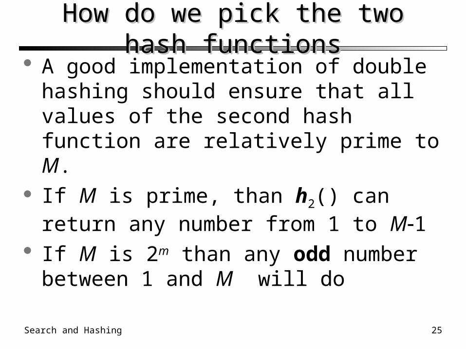
How do we pick the two hash functionsHow do we pick the two hash functions A good implementation of double hashing

should ensure that all values of the second hash function are relatively prime to M.

If M is prime, than h2() can return any number from 1 to M1

If M is 2m than any odd number between 1 and M will do


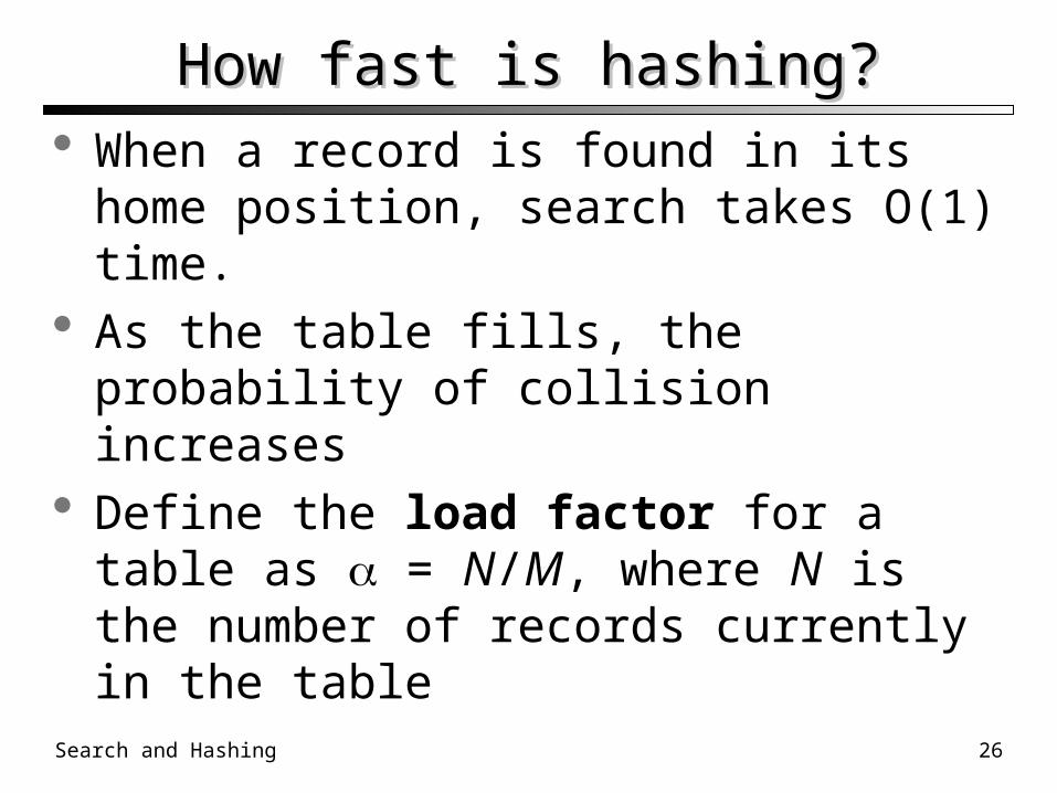
How fast is hashing?How fast is hashing? When a record is found in its home position,

search takes O(1) time. As the table fills, the probability of collision

increases Define the load factor for a table as = N/M,

where N is the number of records currently in the table


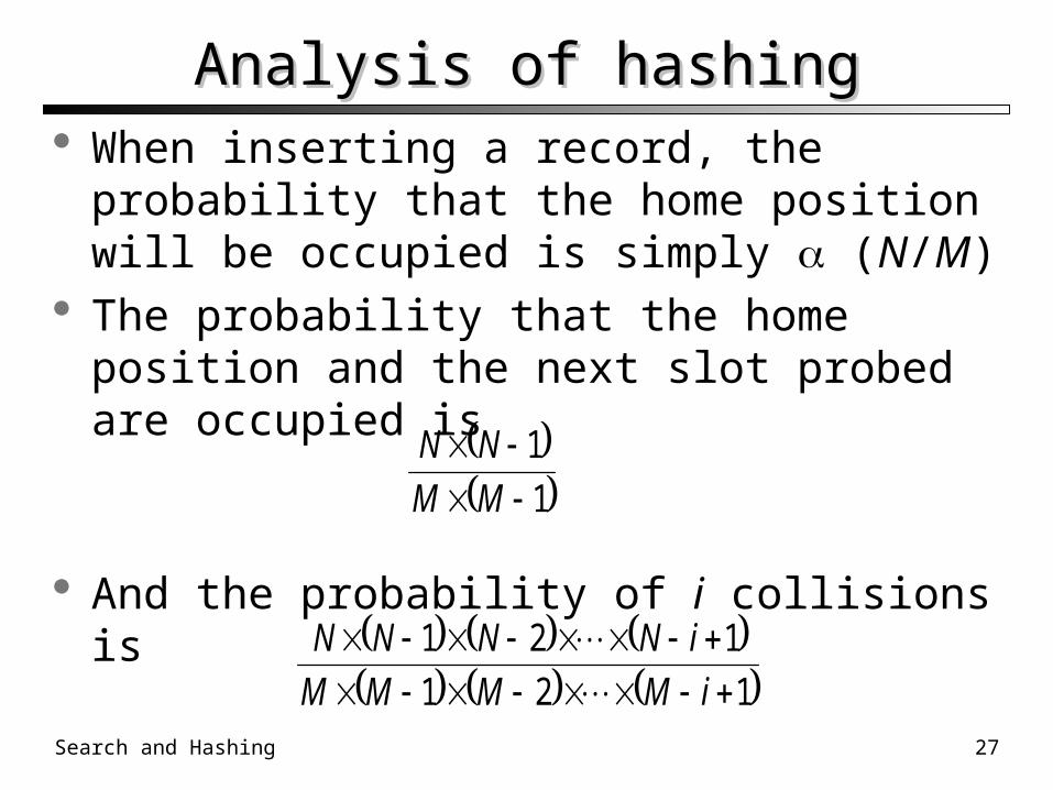
Analysis of hashingAnalysis of hashing When inserting a record, the probability that the

home position will be occupied is simply (N/M)

The probability that the home position and the next slot probed are occupied is

And the probability of i collisions is

1

1

MM

NN

121

121

iMMMM

iNNNN


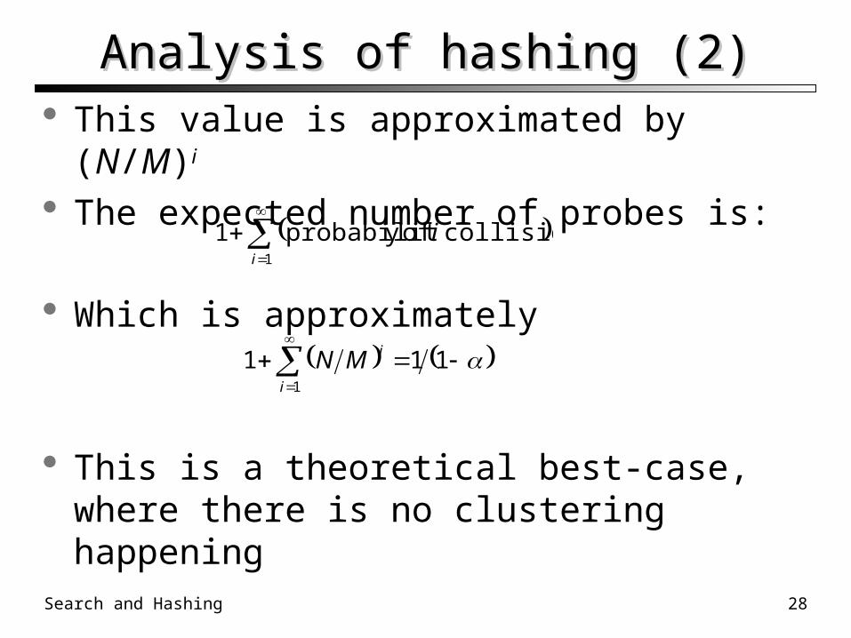
Analysis of hashing (2)Analysis of hashing (2) This value is approximated by (N/M)i

The expected number of probes is:

Which is approximately

This is a theoretical best-case, where there is no clustering happening

1

collisions ofy probabilit1i

i

1

111i

iMN


Hashing PerformanceHashing Performance

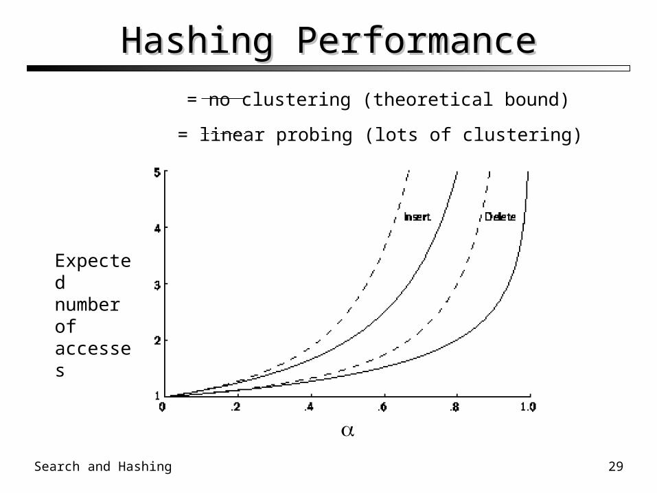
Expected number of accesses

= no clustering (theoretical bound)

= linear probing (lots of clustering)


DeletionDeletion

Deleting a record must not hinder later searches.

Remember, we stop the search through the probe sequence when we find an empty slot.

We do not want to make positions in the hash table unusable because of deletion.


Tombstones (1)Tombstones (1)

Both of these problems can be resolved by placing a special mark in place of the deleted record, called a tombstone.

A tombstone will not stop a search, but that slot can be used for future insertions.


Tombstones (2)Tombstones (2)

Unfortunately, tombstones add to the average path length.

Solutions:1. Local reorganizations to try to shorten the

average path length.2. Periodically rehash the table (by order of

most frequently accessed record).

Download - Searching: Self Organizing Structures and Hashing CS 400/600 – Data Structures

Top Related