1
Revisiting Alpha-Investing: Conditionally Valid
Stepwise Regression
Kory Johnson1, Robert A. Stine1, and Dean P. Foster1
1The Wharton School, University of Pennsylvania
May 16, 2016
Abstract
Valid conditional inference has become a topic of increasing concern. Johnson
et al. (2016) provide a framework for understanding the difficulties presented by
using hypothesis testing to select a model. They also present an algorithm for
performing valid stepwise regression. We extend their results and provide sev-
eral practical improvements which yield an algorithm, Revisiting Alpha-Investing
(RAI), that provides a fast approximation to forward stepwise. RAI performs model
selection in O(np log(n)) time while controlling type-I error and provably finding
signal: it controls the marginal false discovery rate and selects a model that is a
(1 − 1/e) + ε approximation to the best model of the same size. The algorithm
is successful under the assumption of approximate submodularity, which is quite
general and allows for highly correlated explanatory variables. We demonstrate
the adaptability of RAI by using it to search complex interaction spaces in both
simulated and real data.
1 Introduction
We study the problem of selecting predictive features from a large feature space. Our
data consists of n observations of (response, feature) sets, (yi, xi1, . . . , xim), where each
May 16, 2016 DRAFT
arX
iv:1
510.
0632
2v2
[st
at.M
E]
13
May
201
6
2
observation has m associated features. Observations are collected into matrices and the
following model is assumed for our data
Y = Xβ + ε ε ∼ Nn(0, σ2In) (1)
where X is an n × m matrix and Y is an n × 1 response vector. Typically, most of
the elements of β are 0. Hence, generating good predictions requires identifying the
small subset of predictive features. The model (1) proliferates the statistics and machine
learning literature. In modern applications, m is often large, potentially with m �
n, which makes the selection of an appropriate subset of these features essential for
prediction. Algorithms must be fast enough to be computationally feasible and yet must
find signal without over-fitting the data.
The traditional solution to the feature selection problem attempts to minimize the
error sum of squares
ESS(Y ) = ‖Y − Y ‖22
and solves
minβ
ESS(Xβ) s.t. ‖β‖l0 =m∑i=1
I{βi 6=0} ≤ k, (2)
where the number of nonzero features, k, is the desired sparsity. Note that we are not
assuming a sparse representation exists, merely asking for a sparse approximation. In the
statistics literature, this is more commonly posed as a penalized regression:
β0,λ = argminβ {ESS(Xβ) + λ‖β‖l0} (3)
where λ ≥ 0 is a constant. The classical hard thresholding algorithms Cp (Mallows,
1973), AIC (Akaike, 1974), BIC (Schwarz, 1978), and RIC (Foster and George, 1994)
vary λ. Let S ⊂ {1, . . . ,m} indicate the coordinates of a given model so that XS is the
corresponding submatrix of the data. If S∗λ is the optimal set of features for a given λ,
then (3) is solved by ordinary least-squares: βLS = (XTS∗XS∗)
−1XS∗Y .
May 16, 2016 DRAFT

3
Given the combinatorial nature of the constraint, solving (2) quickly becomes infea-
sible as m increases and is NP-hard in general (Natarajan, 1995). One common solution
is to approximate (2) using greedy algorithms such as forward stepwise regression. Let
Si be the features in the forward stepwise model after step i and note that the size of
the model is |Si| = i. The algorithm is initialized with S0 = ∅ and iteratively adds the
variable which yields the largest reduction in ESS. Hence, Si+1 = {Si ∪ j} where
j = arg maxl∈{1,...,m}\Si
ESS(XSi∪lβLSSi∪l).
After the first feature is selected, subsequent models are built having fixed that feature
in the model. S1 is the optimal size-one model, but Si for i ≥ 2 is not guaranteed to be
optimal, because they are forced to include the features identified at previous steps. For
simple examples of this failing see Miller (2002) and for a full characterization of such
issues see Johnson et al. (2015b).
A final model from the forward stepwise path is often identified using cross-validation
or minimizing a criterion such as AIC. The classical rules to stop forward stepwise such as
F-to-enter do not control any robust statistical quantity, because attempting to test the
addition of such a feature uses non-standard and complex distributions (Draper et al.,
1971; Pope and Webster, 1972). Johnson et al. (2016) approximates forward stepwise in
order to provide valid statistical guarantees. We improve upon this method, ensuring the
risk of the selected model is close to that of the stepwise model, even in cases when the
models differ (Theorem 1). In this way, our results can be interpreted as type-II error
control. We also provide the speed and flexibility to use forward stepwise in modern
problems.
There are few provable bounds on how well greedy statistical algorithms perform.
Zhang (2008) provides bounds for a forward-backward selection algorithm, FoBa, but
the algorithm is slower than forward stepwise, limiting its use. Guaranteeing the success
of greedy methods is important as l1-relaxations of (3) such as the Lasso (Tibshirani,
1996) can introduce estimation bias that generates infinitely greater relative risk than
l0-methods (Johnson et al., 2015a). While convex regularizers are computationally con-
May 16, 2016 DRAFT

4
venient, they are less desirable than their non-convex counterparts (Breheny and Huang,
2011). Furthermore, l1-based methods over-estimate the support of β (Zou, 2006). One
potential solution is to use blended, non-convex regularizers such as SCAD (Fan and Li,
2001), to which we will compare out solution in Section 3.
Our solution, given in Section 2, provides performance enhancing modifications to
the valid stepwise procedure identified in Johnson et al. (2016). The resulting procedure,
Revisiting Alpha-Investing (RAI), has a performance guarantee that can be interpreted
as type-II error control as the procedure is guaranteed to find signal. The guarantees of
Section 2.2 are closely related to Das and Kempe (2008, 2011) and the classical result of
Nemhauser et al. (1978) which states that, under suitable assumptions, greedy algorithms
provide a (1− 1/e) approximation of the optimal solution to (2).
Section 2 describes how RAI leverages statistical testing to choose the order in which
features are added to the model. RAI is a “streaming” procedure that sequentially
considers each feature for addition to the model, instead of performing a global search for
the best one. A feature merely needs to be significant enough, and not necessarily the most
significant. It is a thresholding approximation to the greedy algorithm (Badanidiyuru
and Vondrak, 2014). RAI makes multiple, fast passes over the features. No more than
log2(n) passes are required, but in practice we find that 5-7 passes are sufficient regardless
of sample size. Each testing pass identifies those features that meet a required level of
statistical significance. The initial testing pass conducts a strict test for which only
extremely significant features are added to the model. Subsequent passes perform a less
stringent test. RAI is not guaranteed to pick the most significant feature, only one that
is significant enough to pass the test. As such, the final model is built from a series of
approximately greedy choices.
The sequential testing framework of RAI allows the order of tested hypotheses to
be changed as the result of previous tests. This allows for directed searches for data
base queries or identifying polynomials. Section 3 leverages this flexibility to greedily
search high-order interactions spaces. We provide simulations and real data examples to
demonstrate the success of our method.
May 16, 2016 DRAFT
5
RAI enjoys three key properties:
1. It is guaranteed to find signal.
2. It does not over-fit the data by controlling type-I errors; few spurious features are
selected.
3. It is computationally efficient.
By leveraging Variance Inflation Factor Regression (Lin et al., 2011), if the final model
is of size q << min(n, p), the computational complexity of RAI grows at O(np log(n)).
Using the full data requires computing X′y, which takes O(np) time. Therefore, RAI
merely adds a log factor to perform valid model selection.
1.1 Notation
We use notation from the multiple comparisons literature given its connection to RAI.
Consider m null hypotheses, H[m]: H1, . . . , Hm, and their associated p-values, p[m]:
p1, . . . , pm. The hypotheses can be considered to be Hi: βi = 0. Forward stepwise
provides an ordering for testing H[m]. Since our goal is model selection, a feature is
“included” or “added” to the model when the corresponding null hypothesis is rejected.
Define the statistic Ri = 1 if Hi is rejected and the random variable V βi = 1 if this was
a false rejection. The dependence of V βi on β indicates that this is an unknown quantity
which depends on the parameter of interest. Define
R(m) =m∑i=1
Ri, and
V (m) =m∑i=1
V βi .
RAI approximates forward stepwise by making approximately greedy choices of fea-
tures. At each step, forward stepwise sorts the p-values of the m′ remaining features,
p(1) < . . . < p(m′), and selects the feature with the minimum p-value p(1). Instead of per-
forming a full sort, consider using increasing significance thresholds, where hypotheses are
rejected when their p-value falls below a threshold. Johnson et al. (2016) used thresholds
determined by the Holm step-down procedure. The resulting procedure, Revisiting Holm
May 16, 2016 DRAFT
6
(RH), is well-motivated for type-I error control, but can fail to accurately approximate
forward stepwise in some cases.
RH and RAI protect against false-rejections by controlling the marginal False Discov-
ery Rate (mFDR) which is closely related to the False Discovery Rate (Benjamini and
Hochberg, 1995):
Definition 1 (Measures of the Proportion of False Discoveries).
mFDR(m) =E(V (m))
E(R(m)) + 1
FDR(m) = E(V (m)
R(m)
), where
0
0= 0.
In some respects, FDR is preferable to mFDR because it controls a property of a
realized distribution. The ratio V (m)/R(m), while not observed, is the realized propor-
tion of false rejections in a given use of a procedure. FDR controls the expectation of
this quantity. In contrast, E(V (m))/E(R(m)) is not a property of the distribution of the
proportion of false rejections. That being said, FDR and mFDR behave similarly in prac-
tice and mFDR yields a powerful and flexible martingale (Foster and Stine, 2008). This
martingale provides the basis for proofs of type-I error control in a variety of situations.
RH and RAI control mFDR by implementing an alpha-investing strategy (Foster and
Stine, 2008). Alpha-investing rules are similar to alpha-spending rules in that they are
given an initial alpha-wealth and the wealth is spent on hypothesis tests. Wealth is the
allotment of error probability which can be allocated to tests. Bonferroni allocates this
error probability equally over all hypothesis, testing each one at level α/m. In general,
the amount spent on tests can vary. If αi is the amount of wealth spent on test Hi,
FWER is controlled whenm∑i=1
αi = α.
In clinical trials, alpha-spending is useful due to the varying importance of hypotheses.
For example, many studies include both primary and secondary endpoints. The primary
endpoint of a drug trial may be determining if a drug reduces the risk of heart disease.
As this is the most important hypothesis, the majority of the alpha-wealth can be spent
May 16, 2016 DRAFT

7
on it, providing higher power. There are often many secondary endpoints such as testing
if the drug reduces cholesterol or blood pressure. Alpha-spending rules can allocate the
remaining wealth equally over the secondary hypotheses. FWER is controlled and the
varying importance of hypotheses is acknowledged.
Alpha-investing rules are similar to alpha-spending rules except that alpha-investing
rules earn a return ω, a contribution to the alpha-wealth, when tests are rejected. There-
fore the alpha-wealth after testing hypothesis Hi is
Wi+1 = Wi − αi + ωRi
An alpha-investing strategy uses the current wealth and the history of previous rejections
to determine which hypothesis to test and the amount of wealth that should be spent on
it.
From the perspective of alpha-investing, threshold approximations to forward stepwise
spend αi to test each hypothesis on pass i. If a test is rejected, the algorithm earns the
return ω which allows for more passes. The procedure terminates when it runs out of
alpha-wealth.
1.2 Outline
Section 2 improves the Holm thresholds by controlling the risk incurred from making false
selections. Section 2.2 discusses the main performance result in which RAI is shown to
produce a near-optimal approximation of the performance of the best subset of the data.
RAI has additional flexibility beyond merely performing forward stepwise. This flexibility
is demonstrated in Section 3 by adaptively searching high-order interaction spaces using
RAI.
2 Better Threshold Approximation
Threshold approximations to forward stepwise can select different features than stepwise,
reducing performance guarantees. To motivate our new thresholds, consider a threshold
May 16, 2016 DRAFT
8
approximation that is guaranteed to mimic forward stepwise exactly. Suppose the set of
thresholds is iδ, δ > 0 and i = 1, 2, . . .. On the first “pass” through the hypotheses or
“round” of testing, all m p-values are compared to δ. If none fall below this threshold,
a second pass or round is conducted, in which all m p-values are compared to 2δ. The
threshold is increased by δ each round until a hypothesis is rejected and the correspond-
ing feature is added to the model. The stepwise p-values are recomputed according to
their marginal reduction in ESS given the new model, and the process continues.1 For
sufficiently small δ, this procedure selects variables in the same order as forward stepwise.
2.1 Revisiting Alpha Investing
Instead of focusing on identifying the identical features as forward stepwise, we develop
a set of thresholds to control the additional risk incurred from selecting different features
than forward stepwise. These thresholds must initially correspond to stringent tests so
that only extremely significant features are selected. Our significance thresholds corre-
spond to selecting features which reduce the ESS by ESS(Y )/2i, where i indicates the
round of testing. The resulting procedure is provided in Algorithm 1 and is called Revisit-
ing Alpha-Investing (RAI) because it is an alpha-investing strategy that tests hypotheses
multiple times. This results in both practical and theoretical performance improvements
while maintaining type-I error guarantees. The details of the required calculations are
given in the Appendix.
RAI is well defined in any model in which it is possible to test the addition of a
single feature such as generalized linear models. The testing thresholds ensure that the
algorithm closely mimics forward stepwise, which provides performance guarantees. A
precise statement of this comparison is given in Section 2.2.
Approximating stepwise using these thresholds has many practical performance bene-
fits. First, multiple passes can be made without rejections before the algorithm exhausts
its alpha-wealth and terminates. The initial tests are extremely conservative but only
spend tiny amounts of alpha-wealth. Tests rejected in these stages still earn the full return
1If X is orthogonal, p-values do not change between steps. If p-values do change, a conservativeapproach restarts testing with threshold δ.
May 16, 2016 DRAFT
9
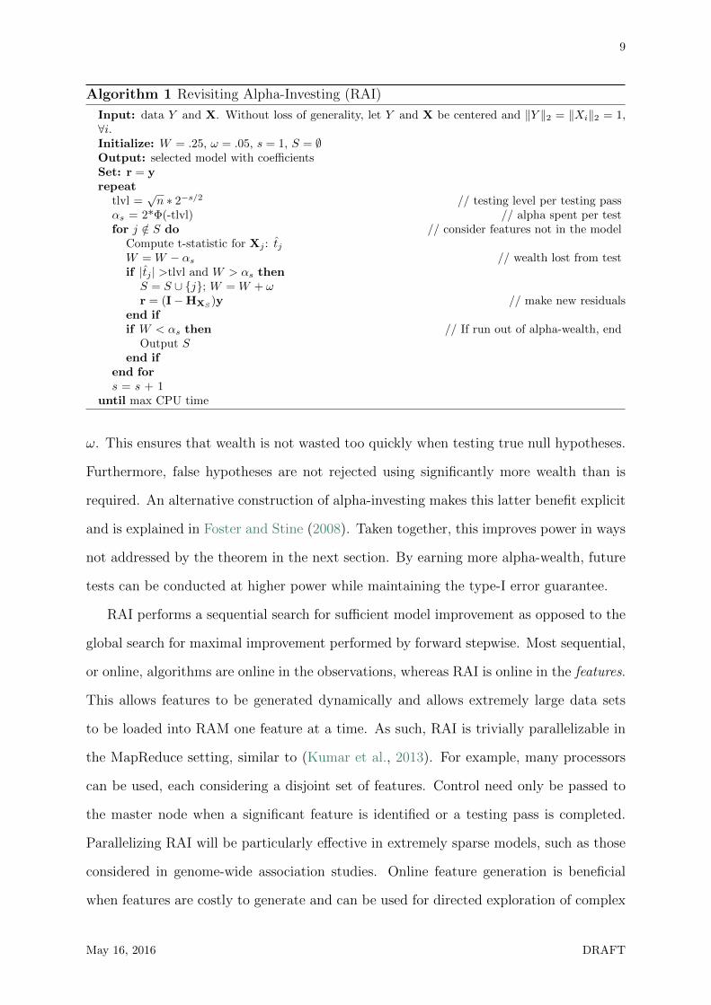
Algorithm 1 Revisiting Alpha-Investing (RAI)
Input: data Y and X. Without loss of generality, let Y and X be centered and ‖Y ‖2 = ‖Xi‖2 = 1,∀i.Initialize: W = .25, ω = .05, s = 1, S = ∅Output: selected model with coefficientsSet: r = yrepeat
tlvl =√n ∗ 2−s/2 // testing level per testing pass
αs = 2*Φ(-tlvl) // alpha spent per testfor j /∈ S do // consider features not in the model
Compute t-statistic for Xj : tjW = W − αs // wealth lost from testif |tj | >tlvl and W > αs thenS = S ∪ {j}; W = W + ωr = (I−HXS
)y // make new residualsend ifif W < αs then // If run out of alpha-wealth, end
Output Send if
end fors = s + 1
until max CPU time
ω. This ensures that wealth is not wasted too quickly when testing true null hypotheses.
Furthermore, false hypotheses are not rejected using significantly more wealth than is
required. An alternative construction of alpha-investing makes this latter benefit explicit
and is explained in Foster and Stine (2008). Taken together, this improves power in ways
not addressed by the theorem in the next section. By earning more alpha-wealth, future
tests can be conducted at higher power while maintaining the type-I error guarantee.
RAI performs a sequential search for sufficient model improvement as opposed to the
global search for maximal improvement performed by forward stepwise. Most sequential,
or online, algorithms are online in the observations, whereas RAI is online in the features.
This allows features to be generated dynamically and allows extremely large data sets
to be loaded into RAM one feature at a time. As such, RAI is trivially parallelizable in
the MapReduce setting, similar to (Kumar et al., 2013). For example, many processors
can be used, each considering a disjoint set of features. Control need only be passed to
the master node when a significant feature is identified or a testing pass is completed.
Parallelizing RAI will be particularly effective in extremely sparse models, such as those
considered in genome-wide association studies. Online feature generation is beneficial
when features are costly to generate and can be used for directed exploration of complex
May 16, 2016 DRAFT
10
spaces. This is particularly useful when querying data base or searching interaction spaces
and is described in Section 3.
Using additional speed improvements provided by variance inflation factor regres-
sion (VIF) (Lin et al., 2011), RAI performs forward stepwise and model selection in
O(np log(n)) time as opposed to the O(np2q2) required for traditional forward stepwise,
where q is the size of the selected model. The log term is an upper bound on the number
of passes through the hypotheses performed by RAI. This is significantly reduced for
large n by recognizing when passes may be skipped. This is possible whenever a full pass
is made without any rejections, as all of the sequential p-values are known. The control
provided by alpha-investing is maintained, because RAI must pay for all of the skipped
tests. Using this computational shortcut, only 5-7 passes are required to select a model
using RAI.
2.2 Performance Guarantee
This subsection bounds the performance of RAI and requires additional notation. Let
[m] = {1, . . . ,m}. For a subset of indices S ⊂ [m], we denote the corresponding columns
of our data matrix as XS, or merely S when the overloaded notation will not cause
confusion. Most of our discussion concerns maximizing the model fit as opposed to
minimizing loss. Our measure of model fit for a set of features XS is the coefficient of
determination, R2, defined as
R2(S) = 1− ESS(XSβS)
ESS(Y )
where Y is the constant vector of the mean response and βS is the least squares estimate of
βS. Maximizing an in-sample criterion such as R2is known to over-fit the data, worsening
out-of-sample performance. To prevent over-fitting, a practical implementation of forward
stepwise requires selecting a model size via cross-validation or criteria such as AIC. RAI
bypasses this problem by controlling mFDR. Without loss of generality, we assume that
our data is centered and normalized such that ‖Y ‖2 = ‖Xi‖2 = 1, ∀i.
May 16, 2016 DRAFT
11
We will often need to consider a feature Xi orthogonal to those currently in the
model, XS. This will be referred to as adjusting Xi for XS. The projection operator
(hat matrix), HXS= HS = XS(XT
SXS)−1XTS , computes the orthogonal projection of a
vector onto the span of the columns of XS. Therefore, Xi adjusted for XS is denoted
Xi.S⊥ = (I −HXS)Xi. This same notation holds for sets of variables: XA adjusted for
XS is XA.S⊥ = (I−HXS)XA.
RAI is proven to perform well if the improvement in fit obtained by adding a set of
features to a model is upper bounded by the sum of the improvements of adding the
features individually. If a large set of features improves the model fit when considered
together, this constraint requires some subsets of those features to improve the fit well.
Consider the improvement in model fit by adding XS to the model XT :
∆T (S) := R2(S ∪ T )− R2(T ).
Letting S = A ∪B, we bound ∆T (S) as
∆T (A) + ∆T (B) ≥ ∆T (S). (4)
If A∪B improves the model fit, equation (4) requires that either A or B improve the
fit. Therefore, signal that is present due to complex relationships among features cannot
be completely hidden when considering subsets of these features. Equation (4) defines a
submodular function:
Definition 2 (Submodular Function). Let F : 2[m] → R be a set function defined on the
the power set of [m]. F is submodular if ∀A,B ⊂ [m]
F (A) + F (B) ≥ F (A ∪B) + F (A ∩B) (5)
This can be rewritten in the style of (4) as
F (A)− F (A ∩B) + F (B)− F (A ∩B) ≥ F (A ∪B)− F (A ∩B)
May 16, 2016 DRAFT

12
⇒ ∆A∩B(A) + ∆A∩B(B) ≥ ∆A∩B(A ∪B),
which considers the impact of A\B and B\A given A∩B. Given (4), it is natural to ap-
proximate the maximizer of a submodular function with a greedy algorithm. We provide
a proof of the performance of RAI by assuming that R2is submodular or approximately
so (made precise below).
In order for these results to hold even more generally, the definition of submodularity
can be relaxed. To do so, iterate (4) until the left hand side is a function of the influ-
ences of individual features and only require the inequality to hold up to a multiplicative
constant γ ≥ 0. For additional simplicity, consider adding the set A = {ai, . . . , al} ⊂ [m]
to the model S. Hence ∆S(ai) is the marginal increase in R2by adding ai to model
S. When data is normalized, ∆S(ai) is the squared partial-correlation between the re-
sponse Y and ai given S: ∆S(ai) = Cor(Y, a⊥i.S)2. Therefore, define the vector of par-
tial correlations as rY,A.S⊥ = Cor(Y,A.S⊥), then the sum of individual contributions to
R2is ‖rY,A.S⊥‖22. Similarly, if we define CA.S⊥ as the correlation matrix of A.S⊥ then
∆S(A) = r′Y,A.S⊥C
−1A.S⊥
rY,A.S⊥ .
Definition 3. (Submodularity Ratio) The submodularity ratio, γsr, of R2with respect to
a set S and k ≥ 1 is
γsr(S, k) = min(T :T∩S=∅,|T |≤k)
r′Y,T.S⊥rY,T.S⊥
r′Y,T.S⊥
C−1T.S⊥
rY,T.S⊥
The minimization identifies the worst case set T to add to the model S. It captures
how much R2can increase by adding T to S (denominator) compared to the combined
benefits of adding its elements to S individually (numerator). If S is the size-k set
selected by forward stepwise, then R2is approximately submodular if γ(S, k) > γ, for
some constant γ > 0. We will refer to data as being approximately submodular if R2is
approximately submodular on the data. R2is submodular if γ(S, 2) ≥ 1 for all S ⊂ [m]
(Johnson et al., 2015b). This definition is similar to that of Das and Kempe (2011).
Our main theoretical result provides a performance guarantee for RAI and is proven
in the Appendix. The result is similar to the in-sample performance guarantees for
May 16, 2016 DRAFT

13
forward stepwise provided by Das and Kempe (2011). Let s index the testing pass, with
sf denoting the first pass in which a hypothesis is rejected. The term γ(Sl, k) is the
submodularity ratio of the selected set of l features, denoted Sl, and S∗k is the set of k
features which minimizes equation (2).
Theorem 1. Algorithm 1 (RAI) selects a set of features Sl of size l such that
R2(Sl) ≥ max
{c1R
2(S∗k)−l∑
j=1
e−(j−1)γSl,k
k 2j−(l+ξf ), c2R2(S∗k)
}
where ci =
(1− e
−lγSl,kik
).
The constant c1 is the optimal constant for greedy approximation, yielding the stan-
dard (1-1/e) approximation for submodular function maximization. As RAI may deviate
from true forward stepwise, the loss incurred can be summarized in two ways. The first
term of the maximization incorporates a small, additive loss that is constructed by consid-
ering the additive cost of selecting a different variable than forward stepwise. It provides
a better bound when k is not small and l ≥ k. The additive error is small, often less than
.02. The cost of errors made during early testing passes are heavily discounted because
the loss of the incorrect selections can be made-up in subsequent steps. The second term
in the maximization incorporates the loss of selecting a different feature than forward
stepwise as a multiplicative error and provides a better bound when l and k are small.
Performance is often better than these bounds indicate, because performance is not a
function of the order in which variables are added, but merely the set of variables in
the final model. If RAI and forward stepwise select the same variables but in a different
order, the bound is merely c1R2(S∗k).
The bound from Theorem 1 does not require the linearity assumption of equation
(1) to hold. It holds uniformly over the true functional relationship between Y and X
because RAI is compared to the best linear approximation of Y given X. The guarantee
is also not a probabilistic statement. Therefore, the ability to compare a model of size l to
a model of size k, where l 6= k, allows practitioners to trade computation time and model
complexity for fit. For example, suppose a selection method selects k features with R2=
May 16, 2016 DRAFT
14
R2∗. RAI can quickly identify a model that is guaranteed to achieve .95R2∗ by selecting
l = 3k features. RAI is designed to determine l = k adaptively, however, which results in
a stronger interpretation of the Theorem 1: RAI produces a near optimal approximation
of the best size-k model, where k is chosen such that little signal remains in unselected
features. The extent to which signal is hidden in the remaining features is a function of
the approximate submodularity of the data (Johnson et al., 2015b).
3 Searching Interaction Spaces
As an application of RAI, we demonstrate a principled method to search interaction
spaces while controlling type-I errors. In this case, submodularity is merely a formalism
of the principle of marginality: if an interaction between two features is included in the
multiple regression, the constituent features should be as well. This reflects a belief that
an interaction is only informative if the marginal terms are as well. RAI can perform a
greedy search for main effects, while maintaining the flexibility to add polynomials to the
model that were not in the original feature space. Therefore, we search interaction spaces
in the following way: run RAI on the marginal data X; for i, j ∈ [m], if Xi and Xj are
rejected, test their interaction by including it in the stepwise routine. This bypasses the
need to explicitly enumerate the interaction space, which is computationally infeasible for
large problems. Furthermore, as our data results indicate, it is highly beneficial to only
consider relevant portions of interaction spaces, as the full space is too complex. This is
addressed in detail below. To demonstrate the success of this routine we provide results
on both simulated and real data.
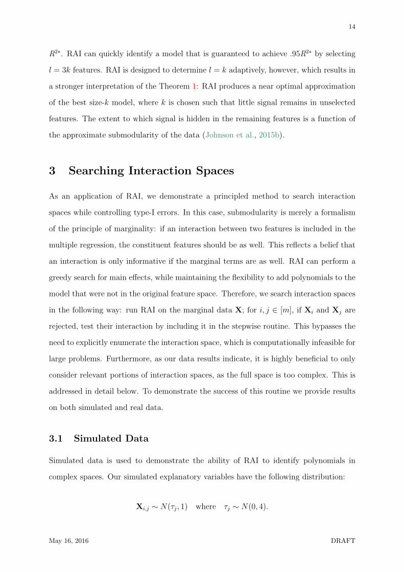
3.1 Simulated Data
Simulated data is used to demonstrate the ability of RAI to identify polynomials in
complex spaces. Our simulated explanatory variables have the following distribution:
Xi,j ∼ N(τj, 1) where τj ∼ N(0, 4).
May 16, 2016 DRAFT
15
The true mean of Y , µY , includes four terms which are polynomials in the first ten
marginal variables:
Y = µY + ε
µY = β1X1X2 + β2X3X24 + β3X5X
36 + β4X7X8X9X10
ε ∼ N(0, I)
The coefficients β1, . . . , β4, are equal given the norm of the interaction and are chosen to
yield a true model R2of approximately .83. The t-statistics of features in the true model
range between 25 and 40.
We first simulate a small-p environment: 2,000 observations with 350 explanatory
features. While our features are simulated independently, the maximum observed cor-
relation is approximately .14. While many competitor algorithms are compared on the
real data, only two are presented here for simplicity. Our goal is to demonstrate the
gains from searching complex spaces using feature selection algorithms. Five algorithms
are compared: RAI searching the interaction space, the Lasso, random forests (Breiman,
2001), the true model, and the mean model. The mean model merely predicts Y in order
to bound the range of reasonable performance between that of the true model and the
mean model. Two Lasso models are compared: the one with minimum cross-validated
error (Lasso.m) and the smallest model with cross-validated error within one standard
deviation of the minimum (Lasso.1). Since the feature space is small, it is possible to
compute the full interaction space of approximately 61,000 variables. Lasso is given
this larger set, while RAI and random forests are only given the 350 marginal variables.
Random forests is included such that comparison can be made to a high-performance,
off-the-shelf procedure that also constructs its own feature space.
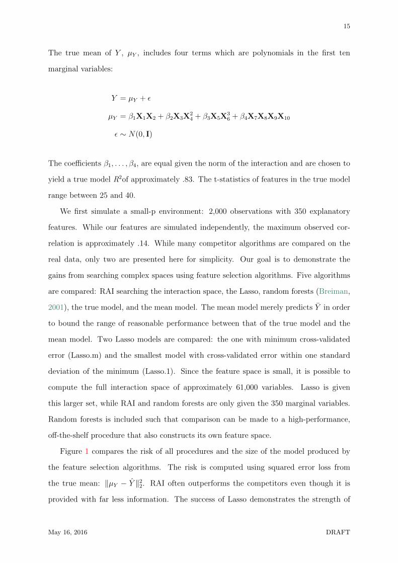
Figure 1 compares the risk of all procedures and the size of the model produced by
the feature selection algorithms. The risk is computed using squared error loss from
the true mean: ‖µY − Y ‖22. RAI often outperforms the competitors even though it is
provided with far less information. The success of Lasso demonstrates the strength of
May 16, 2016 DRAFT
16
(a) Risk (b) Model Size
Figure 1: Small-p results.
correlation in this model. Even though Lasso can only accurately include the interaction
X1X2, it is able to perform reasonably well in some cases. Figure 1 re-samples the data
50 times, creating cases of varying difficulty. Often, difficult cases are challenging for
all algorithms, such that the highest risk data set is the same for all procedures. RAI
performs better than Lasso.m on the majority of cases and almost always outperforms
Lasso.1. The overlapping box plots merely demonstrates the variability in the difficulty
of data sets.
It is also worth comparing the size of the model selected by different procedures.
The Lasso often selects a very large number of variables to account for its inability
to incorporate the correct interactions. As we show more explicitly in the real data
examples, this is a general problem even when the Lasso is provided the higher-order
interactions. Using the model identified by Lasso.1 dramatically reduces model size with
a concomitant increase in loss. Contrast this with RAI, which selects a relatively small
number of features even though its search space is conceptually infinite, as no bounds on
complexity of interactions is imposed. Furthermore, RAI necessarily selects more than
four features in order to identify the higher order terms. For example, in order to identify
the term X7X8X9X10, all four marginal features need to be included as well.
While our results do not focus on speed, it is worth mentioning that RAI easily
May 16, 2016 DRAFT
17
Figure 2: Large-p results.
improves speed by a factor of 10-20 over the Lasso. This is notable since the Lasso is
computed using glmnet (Hastie and Junyang, 2014), a highly optimized Fortran package,
while RAI is coded in R and is geared toward conceptual clarity as opposed to speed.
It also does not implement the improvement provided by VIF (Lin et al., 2011). Even
outside of these considerations, RAI also does not have to compute the full interaction
space.
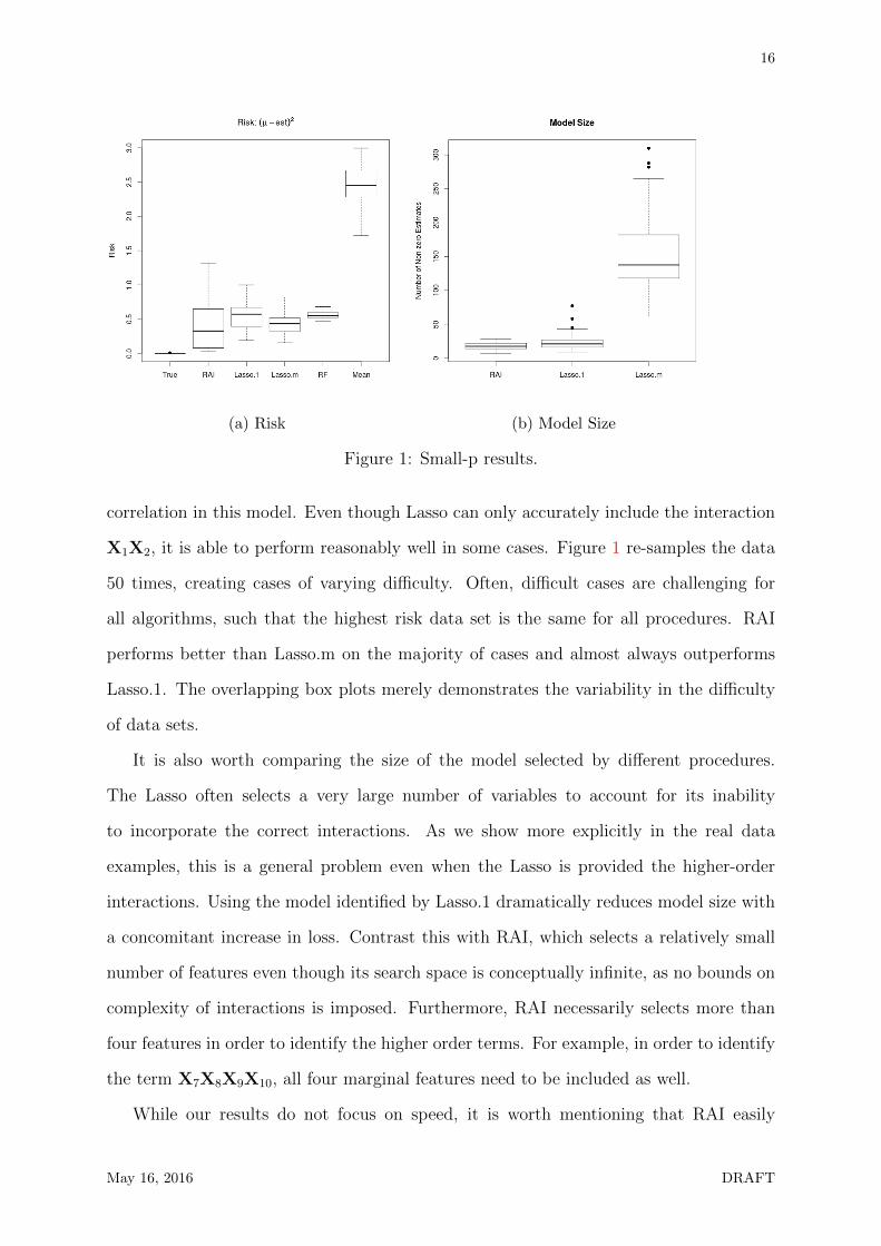
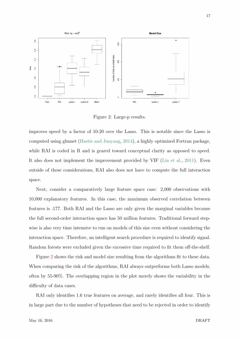
Next, consider a comparatively large feature space case: 2,000 observations with
10,000 explanatory features. In this case, the maximum observed correlation between
features is .177. Both RAI and the Lasso are only given the marginal variables because
the full second-order interaction space has 50 million features. Traditional forward step-
wise is also very time intensive to run on models of this size even without considering the
interaction space. Therefore, an intelligent search procedure is required to identify signal.
Random forests were excluded given the excessive time required to fit them off-the-shelf.
Figure 2 shows the risk and model size resulting from the algorithms fit to these data.
When comparing the risk of the algorithms, RAI always outperforms both Lasso models,
often by 55-90%. The overlapping region in the plot merely shows the variability in the
difficulty of data cases.
RAI only identifies 1.6 true features on average, and rarely identifies all four. This is
in large part due to the number of hypotheses that need to be rejected in order to identify
May 16, 2016 DRAFT
18
an interaction such as X7X8X9X10. At least seven tests must be rejected, starting with
the marginal terms, some second- and third-order interactions, and lastly the true feature.
As the last test of X7X8X9X10 cannot even be conducted until all previous tests have
been rejected, there is a high barrier to identifying such complex interactions. That being
said, significant progress toward this true feature is made in all cases. For example, the
model includes features such as X7X8 and X8X9 or X7X9X10. Therefore, in the small-m
case, the true fitted space is not much larger than that considered by the Lasso. RAI
performs better in this case because it does not need to consider the full complexity of
the 61,000 features in the interaction space.
3.2 Real Data
One may be concerned that the reason RAI outperforms the Lasso in the simulated
scenarios is that RAI is able to search a more complex space. The simulated signal lies in
higher-order polynomials of the features to which Lasso does not have access. While this
itself is an important benefit of our method, we address this concern using a small, real
data set. The results demonstrate that RAI is able to identify the appropriately complex
interaction space. Searching unnecessarily complex spaces worsens performance of the
competitor algorithms.
We use the concrete compressive strength data from the UCI machine learning repos-
itory (Yeh, 1998). This data set was chosen because the response, compressive strength,
is described as a “highly nonlinear function of age and ingredients” such as cement, fly
ash, water, superplasticizer, etc. It is also useful since it has approximately 1000 obser-
vations and only 8 features. A small number of features is needed so that a very large,
higher-order interaction space can be generated. All interactions up to fifth order are
provided to competitor algorithms, in which case there are 1,200 features.
We compare RAI to forward stepwise, Lasso, SCAD (Fan and Li, 2001), and the
Dantzig selector (Candes and Tao, 2007). These are computed in R with the pack-
ages leaps, glmnet, ncvreg, and flare, respectively. Leaps and glmnet are both written
in Fortran with wrappers for R implementation. SCAD uses a non-convex regularizer
May 16, 2016 DRAFT
19
that attempts to blend the benefits of non-convex and convex regularizers. The stepwise
model is chosen by minimizing AIC as this asymptotically selects a model that performs
best among candidate models (Shao, 1997). The leaps package does not actually fit each
model, so if selection with cross-validation is desired, computation time will increase
concordantly. Lasso and SCAD use 10-fold cross-validation to determine the regular-
ization parameter, since this is the default for their estimation functions. As before,
both Lasso.m and Lasso.1 are considered. The regularization parameter for the Dantzig
selector is chosen via 5-fold cross-validation due to its slow run time.
To honestly estimate out-of-sample performance, we create 20 independent splits of
the data into training and test sets. The training data is 5/6 of the full data, and the test
set is the remainder. Each algorithm is fit using the training data; hence, cross-validation
is conducted by splitting the training data again. The test set was only considered after
the model was specified. We compare models using the predictive mean-squared error
(PMSE) on the test set and average model size. Each row in Table 1 indicates the
explanatory variables that the algorithms are provided. For example, the first row shows
the performance results when all algorithms are only given marginal features, while in
subsequent rows the competitor algorithms are given all second order interactions etc.
Both the Stepwise and Dantzig models were excluded for the data set of fifth-order
interactions. The Leaps package was unable to manage the complexity of the space and
other implementations of stepwise proceed far too slowly to even consider being used on
these data. Similarly, the Dantzig selector was too slow and performed too poorly on
smaller feature spaces to warrant its inclusion.
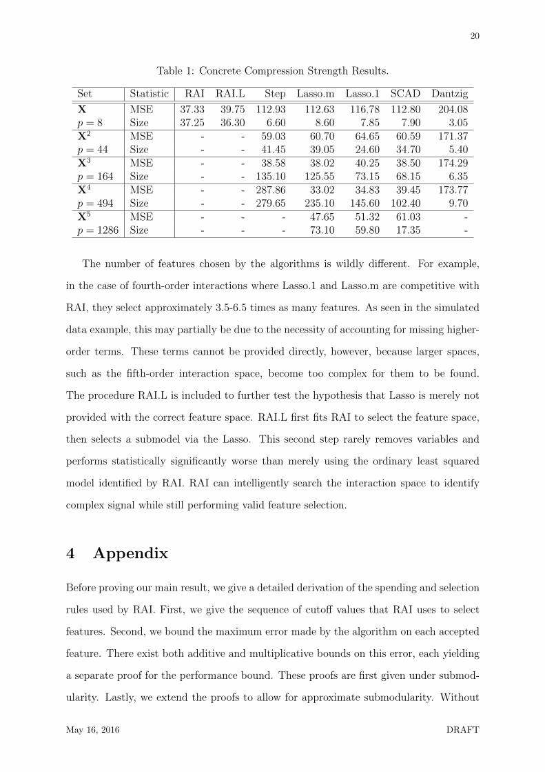
There are several important points in Table 1. As expected, RAI is superior to
other feature selection methods when only considering marginal features; however, we
can adjust for the information differences by giving the competitor algorithms a richer
feature space. Other methods need to be given all fourth-order interactions before they
are competitive with RAI. As further information is provided, however, the performance
of the competitor algorithms worsens. This demonstrates that RAI adaptively determines
the appropriate feature space.
May 16, 2016 DRAFT
20
Table 1: Concrete Compression Strength Results.
Set Statistic RAI RAI.L Step Lasso.m Lasso.1 SCAD Dantzig
X MSE 37.33 39.75 112.93 112.63 116.78 112.80 204.08p = 8 Size 37.25 36.30 6.60 8.60 7.85 7.90 3.05X2 MSE - - 59.03 60.70 64.65 60.59 171.37p = 44 Size - - 41.45 39.05 24.60 34.70 5.40X3 MSE - - 38.58 38.02 40.25 38.50 174.29p = 164 Size - - 135.10 125.55 73.15 68.15 6.35X4 MSE - - 287.86 33.02 34.83 39.45 173.77p = 494 Size - - 279.65 235.10 145.60 102.40 9.70X5 MSE - - - 47.65 51.32 61.03 -p = 1286 Size - - - 73.10 59.80 17.35 -
The number of features chosen by the algorithms is wildly different. For example,
in the case of fourth-order interactions where Lasso.1 and Lasso.m are competitive with
RAI, they select approximately 3.5-6.5 times as many features. As seen in the simulated
data example, this may partially be due to the necessity of accounting for missing higher-
order terms. These terms cannot be provided directly, however, because larger spaces,
such as the fifth-order interaction space, become too complex for them to be found.
The procedure RAI.L is included to further test the hypothesis that Lasso is merely not
provided with the correct feature space. RAI.L first fits RAI to select the feature space,
then selects a submodel via the Lasso. This second step rarely removes variables and
performs statistically significantly worse than merely using the ordinary least squared
model identified by RAI. RAI can intelligently search the interaction space to identify
complex signal while still performing valid feature selection.
4 Appendix
Before proving our main result, we give a detailed derivation of the spending and selection
rules used by RAI. First, we give the sequence of cutoff values that RAI uses to select
features. Second, we bound the maximum error made by the algorithm on each accepted
feature. There exist both additive and multiplicative bounds on this error, each yielding
a separate proof for the performance bound. These proofs are first given under submod-
ularity. Lastly, we extend the proofs to allow for approximate submodularity. Without
May 16, 2016 DRAFT
21
loss of generality, let Y and X be centered and ‖Y ‖2 = ‖Xi‖2 = 1, ∀i.
RAI passes over the features several times, testing them against t-statistic thresholds
that decrease with each pass. Each pass through the full data is indexed by s. RAI
searches for features that result in an increase of (1/2)s in R2for the current model. This
increase is upper bounded by (1/2)(s+i) in terms of R2on the original scale, where i is
the number of features in the current model. Therefore, rejecting multiple hypotheses at
the same level can result in an exponential decrease in residual variation. First, we must
convert this increase in terms of R2to critical values.
If the size of the selected model, is much smaller than the sample size n then the
maximum t-statistic is of order n1/2. Since RAI tests all of the features every pass, the
largest difference in R2of RAI and forward stepwise produced by a single step occurs when
RAI selects a feature whose hypothesis test was barely rejected, while the hypothesis test
of the best feature barely failed being rejected in the previous testing pass. These choices
increase R2by at least (1/2)(s+i) and (1/2)(s+i−1), respectively. The difference decreases by
a multiplicative factor of 1/2 whenever a feature is added or a testing pass is completed.
Hence, the additive loss in terms of R2incurred when selecting a feature is bounded by
R2opt −R2
chosen ≤ 2−(s+i)
We can plug this additive bound into the standard greedy proof of (Nemhauser et al.,
1978), most of which stays the same. The proof is valid for any appropriately bounded
submodular function. Therefore, we use a general f instead of R2. We denote the discrete
derivative of f at S with respect to v as ∆(v|S) := f(S ∪ {v}) − f(S). Let ai be the
feature chosen by RAI at time i, sf the testing pass in which the first feature is chosen,
and δi = f(S∗k)− f(Si).
f(S∗k) ≤ f(Si ∪ S∗k)
= f(Si) +k∑j=1
∆(v∗j |Si ∪ v1, ...vj−1)
≤ f(Si) +∑v∗∈S∗k
(f(Si ∪ v∗)− f(Si))
May 16, 2016 DRAFT
22
≤ f(Si)
+∑v∗∈S∗k
(2−(s+i) + f(Si ∪ ai)− f(Si))
≤ f(Si) + k(2−(s+i) + f(Si+1)− f(Si))
⇒ δi+1 ≤ (1− 1/k)δi + 2−(s+i)
≤ e−(i+1)k f(S∗k) +
i∑j=0
(1− 1/k)j2j−(s+i)
⇒ f(Si+1) ≥(
1− e−lk
)f(S∗k)−
l∑j=1
e−(j−1)
k 2j−(l+s)
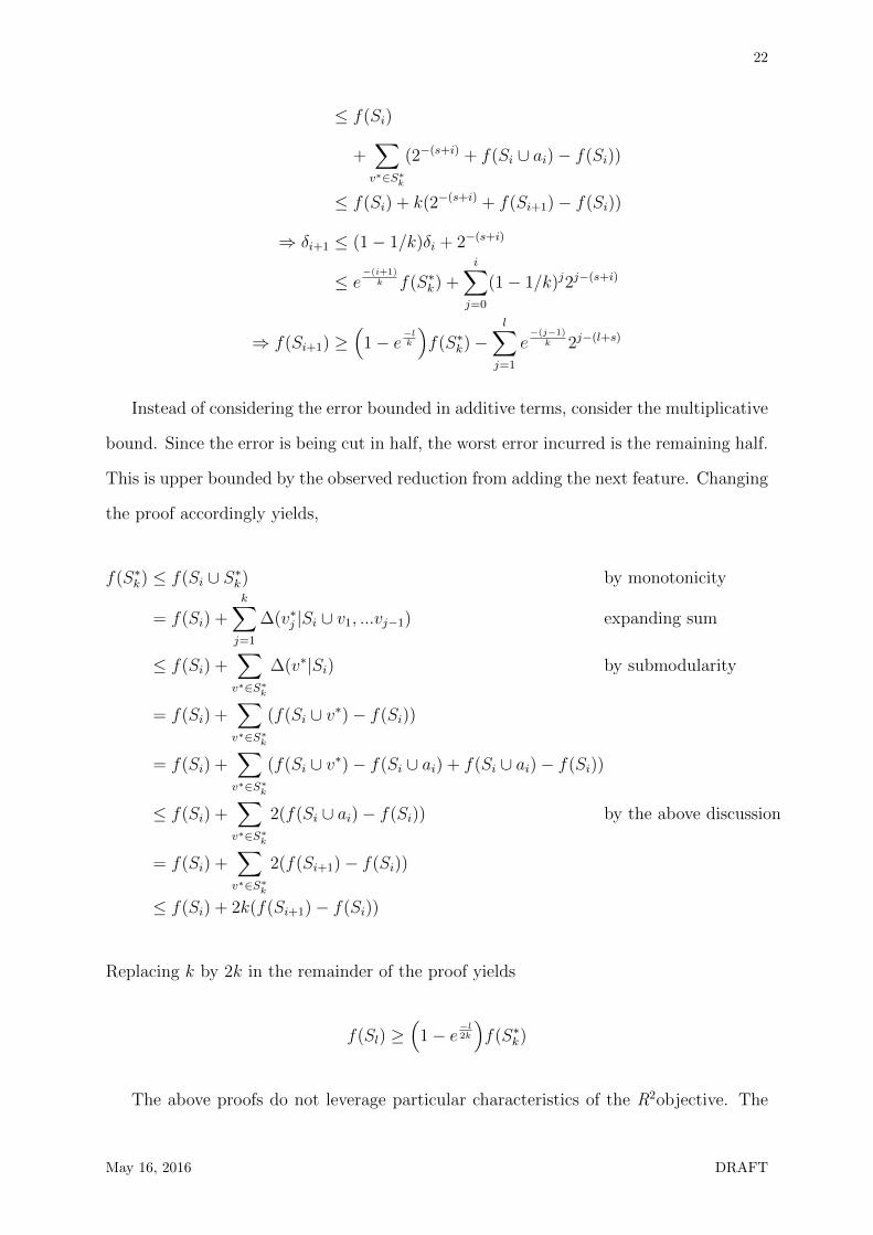
Instead of considering the error bounded in additive terms, consider the multiplicative
bound. Since the error is being cut in half, the worst error incurred is the remaining half.
This is upper bounded by the observed reduction from adding the next feature. Changing
the proof accordingly yields,
f(S∗k) ≤ f(Si ∪ S∗k) by monotonicity
= f(Si) +k∑j=1
∆(v∗j |Si ∪ v1, ...vj−1) expanding sum
≤ f(Si) +∑v∗∈S∗k
∆(v∗|Si) by submodularity
= f(Si) +∑v∗∈S∗k
(f(Si ∪ v∗)− f(Si))
= f(Si) +∑v∗∈S∗k
(f(Si ∪ v∗)− f(Si ∪ ai) + f(Si ∪ ai)− f(Si))
≤ f(Si) +∑v∗∈S∗k
2(f(Si ∪ ai)− f(Si)) by the above discussion
= f(Si) +∑v∗∈S∗k
2(f(Si+1)− f(Si))
≤ f(Si) + 2k(f(Si+1)− f(Si))
Replacing k by 2k in the remainder of the proof yields
f(Sl) ≥(
1− e−l2k
)f(S∗k)
The above proofs do not leverage particular characteristics of the R2objective. The
May 16, 2016 DRAFT
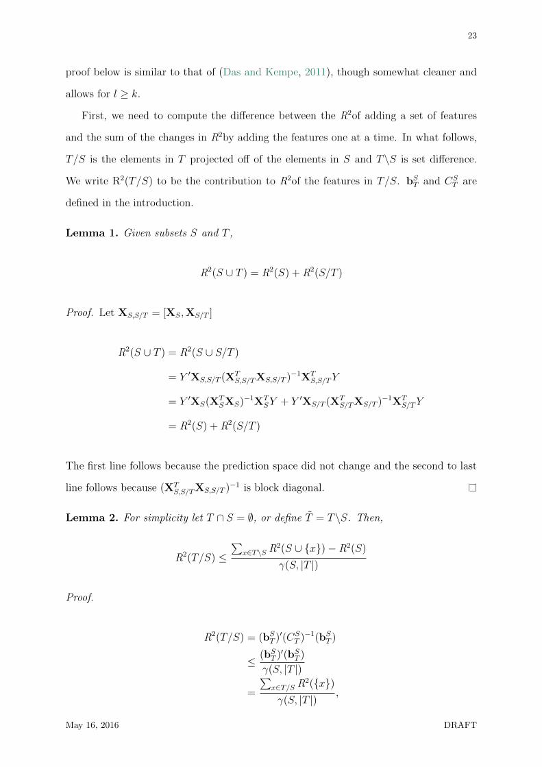
23
proof below is similar to that of (Das and Kempe, 2011), though somewhat cleaner and
allows for l ≥ k.
First, we need to compute the difference between the R2of adding a set of features
and the sum of the changes in R2by adding the features one at a time. In what follows,
T/S is the elements in T projected off of the elements in S and T\S is set difference.
We write R2(T/S) to be the contribution to R2of the features in T/S. bST and CST are
defined in the introduction.
Lemma 1. Given subsets S and T ,
R2(S ∪ T ) = R2(S) + R2(S/T )
Proof. Let XS,S/T = [XS,XS/T ]
R2(S ∪ T ) = R2(S ∪ S/T )
= Y ′XS,S/T (XTS,S/TXS,S/T )−1XT
S,S/TY
= Y ′XS(XTSXS)−1XT
SY + Y ′XS/T (XTS/TXS/T )−1XT
S/TY
= R2(S) + R2(S/T )
The first line follows because the prediction space did not change and the second to last
line follows because (XTS,S/TXS,S/T )−1 is block diagonal.
Lemma 2. For simplicity let T ∩ S = ∅, or define T = T\S. Then,
R2(T/S) ≤∑
x∈T\S R2(S ∪ {x})− R2(S)
γ(S, |T |)
Proof.
R2(T/S) = (bST )′(CST )−1(bST )
≤ (bST )′(bST )
γ(S, |T |)
=
∑x∈T/S R2({x})γ(S, |T |)
,
May 16, 2016 DRAFT
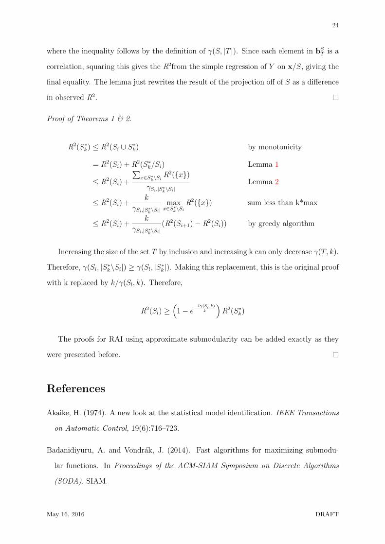
24
where the inequality follows by the definition of γ(S, |T |). Since each element in bST is a
correlation, squaring this gives the R2from the simple regression of Y on x/S, giving the
final equality. The lemma just rewrites the result of the projection off of S as a difference
in observed R2.
Proof of Theorems 1 & 2.
R2(S∗k) ≤ R2(Si ∪ S∗k) by monotonicity
= R2(Si) + R2(S∗k/Si) Lemma 1
≤ R2(Si) +
∑x∈S∗k\Si
R2({x})γSi,|S∗k\Si|
Lemma 2
≤ R2(Si) +k
γSi,|S∗k\Si|max
x∈S∗k\SiR2({x}) sum less than k*max
≤ R2(Si) +k
γSi,|S∗k\Si|(R2(Si+1)− R2(Si)) by greedy algorithm
Increasing the size of the set T by inclusion and increasing k can only decrease γ(T, k).
Therefore, γ(Si, |S∗k\Si|) ≥ γ(Sl, |S∗k |). Making this replacement, this is the original proof
with k replaced by k/γ(Sl, k). Therefore,
R2(Sl) ≥(
1− e−lγ(Sl,k)
k
)R2(S∗k)
The proofs for RAI using approximate submodularity can be added exactly as they
were presented before.
References
Akaike, H. (1974). A new look at the statistical model identification. IEEE Transactions
on Automatic Control, 19(6):716–723.
Badanidiyuru, A. and Vondrak, J. (2014). Fast algorithms for maximizing submodu-
lar functions. In Proceedings of the ACM-SIAM Symposium on Discrete Algorithms
(SODA). SIAM.
May 16, 2016 DRAFT
25
Benjamini, Y. and Hochberg, Y. (1995). Controlling the False Discovery Rate: A Practical
and Powerful Approach to Multiple Testing. Journal of the Royal Statistical Society
Series B (Methodological), 57(1):289–300.
Breheny, P. and Huang, J. (2011). Coordinate descent algorithms for nonconvex penalized
regression, with applications to biological feature selection. Ann. Appl. Stat., 5(1):232–
253.
Breiman, L. (2001). Random Forests. Machine Learning, 45(1):5–32.
Candes, E. and Tao, T. (2007). The Dantzig Selector: Statistical Estimation When p Is
Much Larger than n. The Annals of Statistics, 35(6):pp. 2313–2351.
Das, A. and Kempe, D. (2008). Algorithms for subset selection in linear regression. In
STOC, pages 45–54.
Das, A. and Kempe, D. (2011). Submodular meets Spectral: Greedy Algorithms for
Subset Selection, Sparse Approximation and Dictionary Selection. In Getoor, L. and
Scheffer, T., editors, ICML, pages 1057–1064. Omnipress.
Draper, N. R., Guttman, I., and Kanemasu, H. (1971). The Distribution of Certain
Regression Statistics. Biometrika, 58(2):pp. 295–298.
Fan, J. and Li, R. (2001). Variable selection via nonconcave penalized likelihood and its
oracle properties. Journal of the American Statistical Association, 96(456):1348–1360.
Foster, D. P. and George, E. I. (1994). The Risk Inflation Criterion for Multiple Regres-
sion. The Annals of Statistics, 22(4):pp. 1947–1975.
Foster, D. P. and Stine, R. A. (2008). α-investing: a procedure for sequential control of
expected false discoveries. Journal of the Royal Statistical Society: Series B (Statistical
Methodology), 70(2):429–444.
Hastie, T. and Junyang, Q. (2014). Glmnet Vignette. Technical report, Stanford.
May 16, 2016 DRAFT
26
Johnson, K. D., Brown, L. D., Foster, D. P., and Stine, R. A. (2016). Valid Stepwise
Regression. In Preparation.
Johnson, K. D., Lin, D., Ungar, L. H., Foster, D. P., and Stine, R. A. (2015a). A
Risk Ratio Comparison of l0 and l1 Penalized Regression. ArXiv e-prints. http:
//arxiv.org/abs/1510.06319.
Johnson, K. D., Stine, R. A., and Foster, D. P. (2015b). Submodularity in Statistics:
Comparing the Success of Model Selection Methods. ArXiv e-prints. http://arxiv.
org/abs/1510.06301.
Kumar, R., Moseley, B., Vassilvitskii, S., and Vattani, A. (2013). Fast Greedy Algorithms
in Mapreduce and Streaming. In Proceedings of the Twenty-fifth Annual ACM Sym-
posium on Parallelism in Algorithms and Architectures, SPAA ’13, pages 1–10, New
York, NY, USA. ACM.
Lin, D., Foster, D. P., and Ungar, L. H. (2011). VIF Regression: A Fast Regression Algo-
rithm for Large Data. Journal of the American Statistical Association, 106(493):232–
247.
Mallows, C. L. (1973). Some Comments on CP. Technometrics, 15(4):pp. 661–675.
Miller, A. (2002). Subset Selection in Regression. Monographs on statistics and applied
probability . Chapman and Hall/CRC 2002, 2nd edition.
Natarajan, B. K. (1995). Sparse Approximate Solutions to Linear Systems. SIAM J.
Comput., 24(2):227–234.
Nemhauser, G., Wolsey, L., and Fisher, M. (1978). An analysis of approximations for
maximizing submodular set functions—II. In Balinski, M. and Hoffman, A., editors,
Polyhedral Combinatorics, volume 8 of Mathematical Programming Studies, pages 73–
87. Springer Berlin Heidelberg.
Pope, P. T. and Webster, J. T. (1972). The Use of an F-Statistic in Stepwise Regression
Procedures. Technometrics, 14(2):pp. 327–340.
May 16, 2016 DRAFT
27
Schwarz, G. (1978). Estimating the dimension of a model. The annals of statistics,
6(2):461–464.
Shao, J. (1997). An Asymptotic Theory for Linear Model Selection. Statistica Sinica,
7:221–264.
Tibshirani, R. (1996). Regression shrinkage and selection via the Lasso. Journal of the
Royal Statistical Society. Series B (Methodological), pages 267–288.
Yeh, I.-C. (1998). Modeling of strength of high-performance concrete using artificial
neural networks. Cement and Concrete research, 28(12):1797–1808.
Zhang, T. (2008). Adaptive Forward-Backward Greedy Algorithm for Sparse Learning
with Linear Models. In Koller, D., Schuurmans, D., Bengio, Y., and Bottou, L., editors,
NIPS, pages 1921–1928. Curran Associates, Inc.
Zou, H. (2006). The Adaptive Lasso and Its Oracle Properties. Journal of the American
Statistical Association, 101:1418–1429.
May 16, 2016 DRAFT


