
For copies of this Booklet and of the full Review to be sent to addressesin the Americas, Australasia, or the Far East, visit
http://pdg.lbl.gov/pdgmail
or write toParticle Data GroupMS 50R6008Lawrence Berkeley National LaboratoryBerkeley, CA 94720-8166, USA
From all other areas, visit
http://pdg.lbl.gov/pdgmail
or write toCERN Scientific Information ServiceCH-1211 Geneva 23Switzerland
To make comments or corrections, send e-mail to [email protected]. Weacknowledge all e-mail via e-mail. No reply indicates nonreceipt. Pleasetry again.
Visit our WWW site: http://pdg.lbl.gov/
The publication of the Review of Particle Physics is supported by theDirector, Office of Science, Office of High Energy Physics of the U.S.Department of Energy under Contract No. DE–AC02–05CH11231; by theU.S. National Science Foundation under Agreement No. PHY-0652989;by the European Laboratory for Particle Physics (CERN); by animplementing arrangement between the governments of Japan (MEXT:Ministry of Education, Culture, Sports, Science and Technology) and theUnited States (DOE) on cooperative research and development; and bythe Italian National Institute of Nuclear Physics (INFN).
1
PARTICLE PHYSICS BOOKLET
Extracted from the Review of Particle Physics∗
K.A. Olive et al. (Particle Data Group), Chin. Phys. C, 38, 090001 (2014)
(next edition: July 2016)
Particle Data Group
K.A. Olive, K. Agashe, C. Amsler, M. Antonelli, J.-F. Arguin, D.M. Asner,
H. Baer, H.R. Band, R.M. Barnett, T. Basaglia, C.W. Bauer, J.J. Beatty,
V.I. Belousov, J. Beringer, G. Bernardi, S. Bethke, H. Bichsel, O. Biebel,
E. Blucher, S. Blusk, G. Brooijmans, O. Buchmueller, V. Burkert,
M.A. Bychkov, R.N. Cahn, M. Carena, A. Ceccucci, A. Cerri, D. Chakraborty,
M.-C. Chen, R.S. Chivukula, K. Copic, G. Cowan, O. Dahl, G. D’Ambrosio,
T. Damour, D. de Florian, A. de Gouvea, T. DeGrand, P. de Jong,
G. Dissertori, B.A. Dobrescu, M. Doser, M. Drees, H.K. Dreiner,
D.A. Edwards, S. Eidelman, J. Erler, V.V. Ezhela, W. Fetscher,
B.D. Fields, B. Foster, A. Freitas, T.K. Gaisser, H. Gallagher, L. Garren,
H.-J. Gerber, G. Gerbier, T. Gershon, T. Gherghetta, S. Golwala,
M. Goodman, C. Grab, A.V. Gritsan, C. Grojean, D.E. Groom,
M. Grunewald, A. Gurtu, T. Gutsche, H.E. Haber, K. Hagiwara,
C. Hanhart, S. Hashimoto, Y. Hayato, K.G. Hayes, M. Heffner, B. Heltsley,
J.J. Hernandez-Rey, K. Hikasa, A. Hocker, J. Holder, A. Holtkamp,
J. Huston, J.D. Jackson, K.F. Johnson, T. Junk, M. Kado, D. Karlen,
U.F. Katz, S.R. Klein, E. Klempt, R.V. Kowalewski, F. Krauss, M. Kreps,
B. Krusche, Yu.V. Kuyanov, Y. Kwon, O. Lahav, J. Laiho, P. Langacker,
A. Liddle, Z. Ligeti, C.-J. Lin, T.M. Liss, L. Littenberg, K.S. Lugovsky,
S.B. Lugovsky, F. Maltoni, T. Mannel, A.V. Manohar, W.J. Marciano,
A.D. Martin, A. Masoni, J. Matthews, D. Milstead, P. Molaro, K. Monig,
F. Moortgat, M.J. Mortonson, H. Murayama, K. Nakamura, M. Narain,
P. Nason, S. Navas, M. Neubert, P. Nevski, Y. Nir, L. Pape, J. Parsons,
C. Patrignani, J.A. Peacock, M. Pennington, S.T. Petcov, A. Piepke,
A. Pomarol, A. Quadt, S. Raby, J. Rademacker, G. Raffelt, B.N. Ratcliff,
P. Richardson, A. Ringwald, S. Roesler, S. Rolli, A. Romaniouk,
L.J. Rosenberg, J.L. Rosner, G. Rybka, C.T. Sachrajda, Y. Sakai,
G.P. Salam, S. Sarkar, F. Sauli, O. Schneider, K. Scholberg, D. Scott,
V. Sharma, S.R. Sharpe, M. Silari, T. Sjostrand, P. Skands, J.G. Smith,
G.F. Smoot, S. Spanier, H. Spieler, C. Spiering, A. Stahl, T. Stanev,
S.L. Stone, T. Sumiyoshi, M.J. Syphers, F. Takahashi, M. Tanabashi,
J. Terning, L. Tiator, M. Titov, N.P. Tkachenko, N.A. Tornqvist, D. Tovey,
G. Valencia, G. Venanzoni, M.G. Vincter, P. Vogel, A. Vogt, S.P. Wakely,
W. Walkowiak, C.W. Walter, D.R. Ward, G. Weiglein, D.H. Weinberg,
E.J. Weinberg, M. White, L.R. Wiencke, C.G. Wohl, L. Wolfenstein,
J. Womersley, C.L. Woody, R.L. Workman, A. Yamamoto, W.-M. Yao,
G.P. Zeller, O.V. Zenin, J. Zhang, R.-Y. Zhu, F. Zimmermann, P.A. Zyla
Technical Associates:
G. Harper, V.S. Lugovsky, P. Schaffner
c©2014 Regents of the University of California
∗The full Review lists all the data, with references, used in obtainingthe values given in the Particle Summary Tables. It also containsmuch additional information. Some of the material that does appearin this Booklet is only an abbreviated version of what appears in thefull Review.
2
PARTICLE PHYSICS BOOKLET TABLE OF CONTENTS
1. Physical constants . . . . . . . . . . . . . . . . . . 42. Astrophysical constants . . . . . . . . . . . . . . . . 6
Summary Tables of Particle Physics
Gauge and Higgs bosons . . . . . . . . . . . . . . . . 8Leptons . . . . . . . . . . . . . . . . . . . . . . 14Quarks . . . . . . . . . . . . . . . . . . . . . . 23Mesons . . . . . . . . . . . . . . . . . . . . . . 25Baryons∗ . . . . . . . . . . . . . . . . . . . . . 150Searches . . . . . . . . . . . . . . . . . . . . . . 179Tests of conservation laws∗ . . . . . . . . . . . . . . 183
Reviews, Tables, and Plots
9. Quantum chromodynamics ∗ . . . . . . . . . . . . . 18810. Electroweak model and constraints on new physics ∗ . . 19111. Status of Higgs boson physics ∗ . . . . . . . . . . . . 20012. Cabibbo-Kobayashi-Maskawa quark mixing matrix ∗ . . 20113. CP violation ∗ . . . . . . . . . . . . . . . . . . . 20814. Neutrino mass, mixing and oscillations ∗ . . . . . . . . 21115. Quark model ∗ . . . . . . . . . . . . . . . . . . . 21816. Grand unified theories ∗ . . . . . . . . . . . . . . . 22119. Structure functions ∗ . . . . . . . . . . . . . . . . 22622. Big-bang cosmology ∗ . . . . . . . . . . . . . . . . 23124. The cosmological parameters ∗ . . . . . . . . . . . . 23725. Dark matter ∗ . . . . . . . . . . . . . . . . . . . 24126. Dark energy ∗ . . . . . . . . . . . . . . . . . . . 24427. Cosmic microwave background ∗ . . . . . . . . . . . 24528. Cosmic rays ∗ . . . . . . . . . . . . . . . . . . . 24829. Accelerator physics of colliders ∗ . . . . . . . . . . . 24930. High-energy collider parameters ∗ . . . . . . . . . . . 25032. Passage of particles through matter ∗ . . . . . . . . . 25133. Particle detectors at accelerators ∗ . . . . . . . . . . 26634. Particle detectors for non-accelerator physics ∗ . . . . . 27835. Radioactivity and radiation protection ∗ . . . . . . . . 28536. Commonly used radioactive sources . . . . . . . . . . 28737. Probability ∗ . . . . . . . . . . . . . . . . . . . . 28938. Statistics ∗ . . . . . . . . . . . . . . . . . . . . . 29343. Clebsch-Gordan coefficients, spherical harmonics,
and d functions . . . . . . . . . . . . . . . . . . 30746. Kinematics ∗ . . . . . . . . . . . . . . . . . . . . 30948. Cross-section formulae for specific processes ∗ . . . . . 31850. Plots of cross sections and related quantities ∗ . . . . . 3236. Atomic and nuclear properties of materials ∗ . . . . . . 3244. Periodic table of the elements . . . . . . inside back cover
∗Abridged from the full Review of Particle Physics.
3
The following are found only in the full Review and on the Web:
http://pdg.lbl.gov
3. International System of Units (SI)5. Electronic structure of the elements7. Electromagnetic relations8. Naming scheme for hadrons
17. Heavy-quark & soft-collinear effective theory18. Lattice quantum chromodynamics20. Fragmentation functions in e+e−, ep and pp collisions21. Experimental tests of gravitational theory23. Big-bang nucleosynthesis31. Neutrino beam lines at proton synchrotrons39. Monte Carlo techniques40. Monte Carlo event generators41. Monte Carlo neutrino event generators42. Monte Carlo particle numbering scheme44. SU(3) isoscalar factors and representation matrices45. SU(n) multiplets and Young diagrams47. Resonances49. Neutrino cross-section measurements
41.Physica
lco
nsta
nts
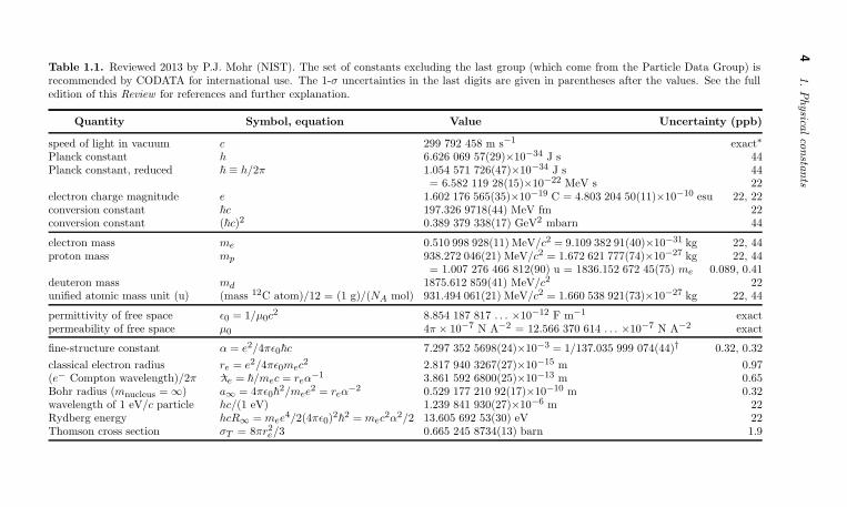
Table 1.1. Reviewed 2013 by P.J. Mohr (NIST). The set of constants excluding the last group (which come from the Particle Data Group) isrecommended by CODATA for international use. The 1-σ uncertainties in the last digits are given in parentheses after the values. See the fulledition of this Review for references and further explanation.
Quantity Symbol, equation Value Uncertainty (ppb)
speed of light in vacuum c 299 792 458 m s−1 exact∗
Planck constant h 6.626 069 57(29)×10−34 J s 44Planck constant, reduced ~ ≡ h/2π 1.054 571 726(47)×10−34 J s 44
= 6.582 119 28(15)×10−22 MeV s 22electron charge magnitude e 1.602 176 565(35)×10−19 C = 4.803 204 50(11)×10−10 esu 22, 22conversion constant ~c 197.326 9718(44) MeV fm 22conversion constant (~c)2 0.389 379 338(17) GeV2 mbarn 44
electron mass me 0.510 998 928(11) MeV/c2 = 9.109 382 91(40)×10−31 kg 22, 44proton mass mp 938.272 046(21) MeV/c2 = 1.672 621 777(74)×10−27 kg 22, 44
= 1.007 276 466 812(90) u = 1836.152 672 45(75) me 0.089, 0.41deuteron mass md 1875.612 859(41) MeV/c2 22unified atomic mass unit (u) (mass 12C atom)/12 = (1 g)/(NA mol) 931.494 061(21) MeV/c2 = 1.660 538 921(73)×10−27 kg 22, 44
permittivity of free space ǫ0 = 1/µ0c2 8.854 187 817 . . . ×10−12 F m−1 exact
permeability of free space µ0 4π × 10−7 N A−2 = 12.566 370 614 . . . ×10−7 N A−2 exact
fine-structure constant α = e2/4πǫ0~c 7.297 352 5698(24)×10−3 = 1/137.035 999 074(44)† 0.32, 0.32
classical electron radius re = e2/4πǫ0mec2 2.817 940 3267(27)×10−15 m 0.97
(e− Compton wavelength)/2π −λe = ~/mec = reα−1 3.861 592 6800(25)×10−13 m 0.65
Bohr radius (mnucleus = ∞) a∞ = 4πǫ0~2/mee
2 = reα−2 0.529 177 210 92(17)×10−10 m 0.32
wavelength of 1 eV/c particle hc/(1 eV) 1.239 841 930(27)×10−6 m 22Rydberg energy hcR∞ = mee
4/2(4πǫ0)2~2 = mec
2α2/2 13.605 692 53(30) eV 22Thomson cross section σT = 8πr2
e/3 0.665 245 8734(13) barn 1.9
1.Physica
lco
nsta
nts
5
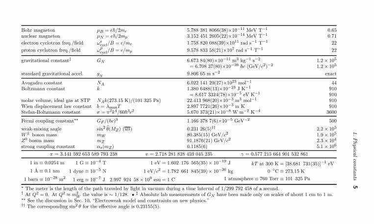
Bohr magneton µB = e~/2me 5.788 381 8066(38)×10−11 MeV T−1 0.65nuclear magneton µN = e~/2mp 3.152 451 2605(22)×10−14 MeV T−1 0.71
electron cyclotron freq./field ωecycl/B = e/me 1.758 820 088(39)×1011 rad s−1 T−1 22
proton cyclotron freq./field ωpcycl
/B = e/mp 9.578 833 58(21)×107 rad s−1 T−1 22
gravitational constant‡ GN 6.673 84(80)×10−11 m3 kg−1 s−2 1.2 × 105
= 6.708 37(80)×10−39~c (GeV/c2)−2 1.2 × 10⁵
standard gravitational accel. gN
9.806 65 m s−2 exact
Avogadro constant NA 6.022 141 29(27)×1023 mol−1 44Boltzmann constant k 1.380 6488(13)×10−23 J K−1 910
= 8.617 3324(78)×10−5 eV K−1 910molar volume, ideal gas at STP NAk(273.15 K)/(101 325 Pa) 22.413 968(20)×10−3 m3 mol−1 910Wien displacement law constant b = λmaxT 2.897 7721(26)×10−3 m K 910Stefan-Boltzmann constant σ = π2k4/60~
3c2 5.670 373(21)×10−8 W m−2 K−4 3600
Fermi coupling constant∗∗ GF /(~c)3 1.166 378 7(6)×10−5 GeV−2 500
weak-mixing angle sin2 θ(MZ) (MS) 0.231 26(5)†† 2.2 × 10⁵
W± boson mass mW 80.385(15) GeV/c2 1.9 × 10⁵
Z0 boson mass mZ 91.1876(21) GeV/c2 2.3 × 10⁴
strong coupling constant αs(mZ) 0.1185(6) 5.1 × 10⁶
π = 3.141 592 653 589 793 238 e = 2.718 281 828 459 045 235 γ = 0.577 215 664 901 532 861
1 in ≡ 0.0254 m
1 A ≡ 0.1 nm
1 barn ≡ 10−28 m2
1 G ≡ 10−4 T
1 dyne ≡ 10−5 N
1 erg ≡ 10−7 J
1 eV = 1.602 176 565(35)× 10−19 J
1 eV/c2 = 1.782 661 845(39)× 10−36 kg
2.997 924 58 × 109 esu = 1 C
kT at 300 K = [38.681 731(35)]−1 eV
0 C ≡ 273.15 K
1 atmosphere ≡ 760 Torr ≡ 101 325 Pa
∗ The meter is the length of the path traveled by light in vacuum during a time interval of 1/299 792 458 of a second.† At Q2 = 0. At Q2
≈ m2W the value is ∼ 1/128. •
‡ Absolute lab measurements of GN have been made only on scales of about 1 cm to 1 m.∗∗ See the discussion in Sec. 10, “Electroweak model and constraints on new physics.”†† The corresponding sin2 θ for the effective angle is 0.23155(5).
62.A
strophysica
lco
nsta
nts
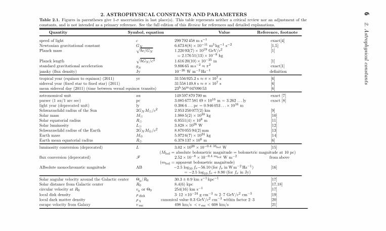
2. ASTROPHYSICAL CONSTANTS AND PARAMETERS
Table 2.1. Figures in parentheses give 1-σ uncertainties in last place(s). This table represents neither a critical review nor an adjustment of theconstants, and is not intended as a primary reference. See the full edition of this Review for references and detailed explanations.
Quantity Symbol, equation Value Reference, footnote
speed of light c 299 792 458 m s−1 exact[4]Newtonian gravitational constant GN 6.673 8(8)× 10−11 m3 kg−1 s−2 [1,5]Planck mass
√
~c/GN 1.220 93(7)× 1019 GeV/c2 [1]= 2.176 51(13)× 10−8 kg
Planck length√
~GN/c3 1.616 20(10)× 10−35 m [1]standard gravitational acceleration g
N9.806 65 m s−2
≈ π2 exact[1]
jansky (flux density) Jy 10−26 W m−2 Hz−1 definition
tropical year (equinox to equinox) (2011) yr 31 556 925.2 s ≈ π × 107 s [6]sidereal year (fixed star to fixed star) (2011) 31 558 149.8 s ≈ π × 107 s [6]mean sidereal day (2011) (time between vernal equinox transits) 23h 56m 04.s090 53 [6]
astronomical unit au 149 597 870 700 m exact [7]parsec (1 au/1 arc sec) pc 3.085 677 581 49× 1016 m = 3.262 . . . ly exact [8]light year (deprecated unit) ly 0.306 6 . . . pc = 0.946 053 . . .× 1016 mSchwarzschild radius of the Sun 2GNM⊙/c2 2.953 250 077(2) km [9]Solar mass M⊙ 1.988 5(2)× 1030 kg [10]Solar equatorial radius R⊙ 6.9551(4)× 108 m [11]Solar luminosity L⊙ 3.828 × 1026 W [12]Schwarzschild radius of the Earth 2GNM⊕/c2 8.870 055 94(2)mm [13]Earth mass M⊕ 5.972 6(7)× 1024 kg [14]Earth mean equatorial radius R⊕ 6.378 137× 106 m [6]
luminosity conversion (deprecated) L 3.02 × 1028× 10−0.4 Mbol W [15]
(Mbol = absolute bolometric magnitude = bolometric magnitude at 10 pc)flux conversion (deprecated) F 2.52 × 10−8
× 10−0.4 mbol W m−2 from above(mbol = apparent bolometric magnitude)
ABsolute monochromatic magnitude AB −2.5 log10 fν−56.10 (for fν in Wm−2 Hz−1) [16]= −2.5 log10 fν + 8.90 (for fν in Jy)
Solar angular velocity around the Galactic center Θ0/R0 30.3 ± 0.9 km s−1 kpc−1 [17]
Solar distance from Galactic center R0 8.4(6) kpc [17,18]circular velocity at R0 v
0or Θ0 254(16) km s−1 [17]
local disk density ρ disk 3–12 ×10−24 g cm−3≈ 2–7 GeV/c2 cm−3 [19]
local dark matter density ρ χ canonical value 0.3 GeV/c2 cm−3 within factor 2–3 [20]escape velocity from Galaxy v esc 498 km/s < v esc < 608 km/s [21]
2.A
strophysica
lco
nsta
nts
7
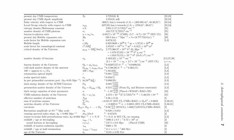
present day CMB temperature T0 2.7255(6) K [22,23]present day CMB dipole amplitude 3.355(8) mK [22,24]Solar velocity with respect to CMB 369(1) km/s towards (ℓ, b) = (263.99(14), 48.26(3)) [22,24]Local Group velocity with respect to CMB vLG 627(22) km/s towards (ℓ, b) = (276(3), 30(3)) [22,24]entropy density/Boltzmann constant s/k 2 891.2 (T/2.7255)3 cm−3 [25]number density of CMB photons nγ 410.7(T/2.7255)3 cm−3 [25]baryon-to-photon ratio η = nb/nγ 6.05(7)×10−10 (CMB); (5.7 − 6.7)×10−10 (95% CL) [26]present day Hubble expansion rate H0 100 h km s−1 Mpc−1 = h×(9.777 752 Gyr)−1 [29]scale factor for Hubble expansion rate h 0.673(12) [2,3]Hubble length c/H0 0.925 0629×1026h−1 m = 1.37(2)×1026 mscale factor for cosmological constant c2/3H2
0 2.85247× 1051 h−2 m2 = 6.3(2) × 1051 m2
critical density of the Universe ρcrit = 3H20/8πGN 2.775 366 27× 1011 h2 M⊙Mpc−3
= 1.878 47(23)× 10−29 h2 g cm−3
= 1.053 75(13)× 10−5 h2 (GeV/c2) cm−3
number density of baryons nb 2.482(32)× 10−7 cm−3 [2,3,27,28](2.1 × 10−7 < nb < 2.7 × 10−7) cm−3 (95% CL) η × nγ
baryon density of the Universe Ωb = ρb/ρcrit‡ 0.02207(27)h−2 = † 0.0499(22) [2,3]
cold dark matter density of the universe Ωcdm = ρcdm/ρcrit‡ 0.1198(26)h−2 = † 0.265(11) [2,3]
100 × approx to r∗/DA 100 × θMC‡ 1.0413(6) [2,3]
reionization optical depth τ ‡ 0.091+0.013−0.014 [2,3]
scalar spectral index ns‡ 0.958(7) [2,3]
ln pwr primordial curvature pert. (k0=0.05 Mpc−1) ln(1010∆2R) ‡ 3.090(25) [2,3]
dark energy density of the ΛCDM Universe ΩΛ 0.685+0.017−0.016 [2,3]
pressureless matter density of the Universe Ωm = Ωcdm +Ωb 0.315+0.016−0.017 (From ΩΛ and flatness constraint) [2,3]
dark energy equation of state parameter w ♯−1.10+0.08
−0.07 (Planck+WMAP+BAO+SN) [32]
CMB radiation density of the Universe Ωγ = ργ/ρc 2.473× 10⁻⁵(T/2.7255)4 h−2 = 5.46(19)×10−5 [25]
effective number of neutrinos Neff† 3.36 ± 0.34 [2]
sum of neutrino masses∑
mν <0.23 eV (95% CL; CMB+BAO) ⇒ Ωνh2 < 0.0025 [2,30,31]neutrino density of the Universe Ων < 0.0025 h−2
⇒ < 0.0055 (95% CL;CMB+BAO) [2,30,31]curvature Ωtot= Ωm + . . . + ΩΛ
♯ 0.96+0.4−0.5 (95%CL); 1.000(7)(95%CL;CMB+BAO) [2]
fluctuation amplitude at 8h−1 Mpc scale σ8† 0.828± 0.012 [2,3]
running spectral index slope, k0 = 0.002 Mpc−1 dns/d ln k ♯−0.015(9) [2]
tensor-to-scalar field perturbations ratio, k0=0.002 Mpc−1 r = T/S ♯ < 0.11 at 95% CL; no running [2,3]redshift / age at decoupling zdec / t∗
† 1090.2± 0.7 / † 3.72 × 10⁵ yr [2]sound horizon at decoupling rs(z∗)
† 147.5± 0.6 Mpc (Planck CMB) [32]redshift of matter-radiation equality zeq
† 3360± 70 [2]
redshift / age at half reionization zreion / treion† 11.1 ± 1.1 / † 462 Myr [2]
age of the Universe t0† 13.81± 0.05 Gyr [2]
8888 Summary Tables of Parti le PropertiesSUMMARY TABLES OF PARTICLE PROPERTIES
Extracted from the Particle Listings of the
Review of Particle Physics
K.A. Olive et al. (PDG), Chin. Phys. C, 38, 090001 (2014)Available at http://pdg.lbl.gov
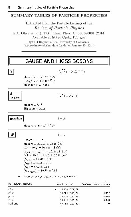
c©2014 Regents of the University of California(Approximate closing date for data: January 15, 2014)GAUGE AND HIGGS BOSONSGAUGE AND HIGGS BOSONSGAUGE AND HIGGS BOSONSGAUGE AND HIGGS BOSONS
γγγγ I (JPC ) = 0,1(1−−)Mass m < 1× 10⁻¹⁸ eVCharge q < 1× 10⁻³⁵ eMean life τ = Stableggggor gluonor gluonor gluonor gluon I (JP ) = 0(1−)Mass m = 0 [aSU(3) olor o tetgravitongravitongravitongraviton J = 2Mass m < 6× 10⁻³² eVWWWW J = 1Charge = ±1 eMass m = 80.385 ± 0.015 GeVmZ − mW = 10.4 ± 1.6 GeVmW+ − mW− = −0.2 ± 0.6 GeVFull width = 2.085 ± 0.042 GeV⟨Nπ±
⟩ = 15.70 ± 0.35⟨NK±
⟩ = 2.20 ± 0.19⟨Np⟩ = 0.92 ± 0.14⟨N harged⟩ = 19.39 ± 0.08W− modes are harge onjugates of the modes below. pW+ DECAY MODESW+ DECAY MODESW+ DECAY MODESW+ DECAY MODES Fra tion (i /) Conden e level (MeV/ )
ℓ+ν [b (10.86± 0.09) % e+ ν (10.71± 0.16) % 40192µ+ν (10.63± 0.15) % 40192τ+ ν (11.38± 0.21) % 40173hadrons (67.41± 0.27) %
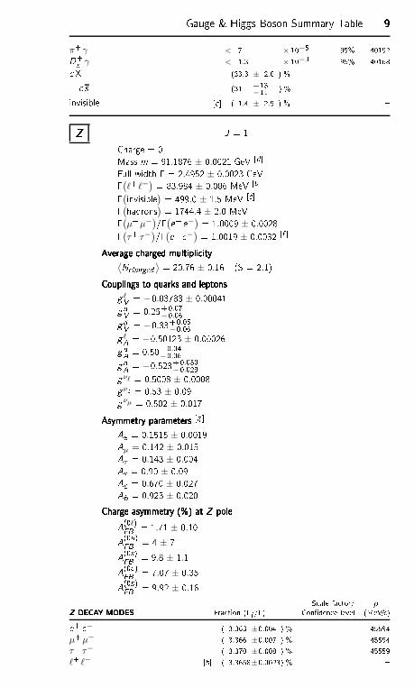
Gauge & Higgs Boson Summary Table 9999π+ γ < 7 × 10⁻⁵ 95% 40192D+s γ < 1.3 × 10⁻³ 95% 40168 X (33.3 ± 2.6 ) % s (31 +13
−11 ) % invisible [ ( 1.4 ± 2.9 ) % ZZZZ J = 1Charge = 0Mass m = 91.1876 ± 0.0021 GeV [dFull width = 2.4952 ± 0.0023 GeV(ℓ+ ℓ−) = 83.984 ± 0.086 MeV [b(invisible) = 499.0 ± 1.5 MeV [e(hadrons) = 1744.4 ± 2.0 MeV(µ+µ−)/(e+ e−) = 1.0009 ± 0.0028(τ+ τ−)/(e+ e−) = 1.0019 ± 0.0032 [f Average harged multipli ityAverage harged multipli ityAverage harged multipli ityAverage harged multipli ity
⟨N harged ⟩ = 20.76 ± 0.16 (S = 2.1)Couplings to quarks and leptonsCouplings to quarks and leptonsCouplings to quarks and leptonsCouplings to quarks and leptonsg ℓV = −0.03783 ± 0.00041guV = 0.25+0.07−0.06gdV = −0.33+0.05
−0.06g ℓA = −0.50123 ± 0.00026guA = 0.50+0.04−0.06gdA = −0.523+0.050
−0.029gνℓ = 0.5008 ± 0.0008gνe = 0.53 ± 0.09gνµ = 0.502 ± 0.017Asymmetry parametersAsymmetry parametersAsymmetry parametersAsymmetry parameters [g Ae = 0.1515 ± 0.0019Aµ = 0.142 ± 0.015Aτ = 0.143 ± 0.004As = 0.90 ± 0.09A = 0.670 ± 0.027Ab = 0.923 ± 0.020Charge asymmetry (%) at Z poleCharge asymmetry (%) at Z poleCharge asymmetry (%) at Z poleCharge asymmetry (%) at Z poleA(0ℓ)FB = 1.71 ± 0.10A(0u)FB = 4 ± 7A(0s)FB = 9.8 ± 1.1A(0 )FB = 7.07 ± 0.35A(0b)FB = 9.92 ± 0.16 S ale fa tor/ pZ DECAY MODESZ DECAY MODESZ DECAY MODESZ DECAY MODES Fra tion (i /) Conden e level (MeV/ )e+ e− ( 3.363 ±0.004 ) % 45594µ+µ− ( 3.366 ±0.007 ) % 45594τ+ τ− ( 3.370 ±0.008 ) % 45559ℓ+ ℓ− [b ( 3.3658±0.0023) %
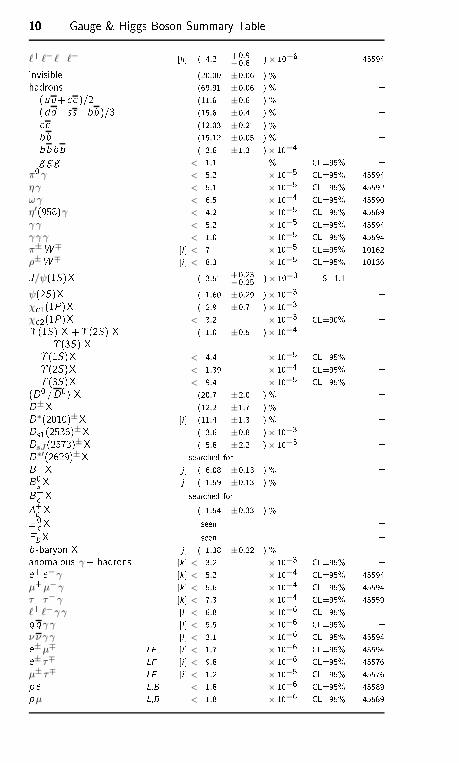
10101010 Gauge & Higgs Boson Summary Tableℓ+ ℓ− ℓ+ ℓ− [h ( 4.2 +0.9
−0.8 )× 10−6 45594invisible (20.00 ±0.06 ) % hadrons (69.91 ±0.06 ) % (uu+ )/2 (11.6 ±0.6 ) % (dd+ss+bb )/3 (15.6 ±0.4 ) % (12.03 ±0.21 ) % bb (15.12 ±0.05 ) % bbbb ( 3.6 ±1.3 )× 10−4 g g g < 1.1 % CL=95% π0 γ < 5.2 × 10⁻⁵ CL=95% 45594ηγ < 5.1 × 10⁻⁵ CL=95% 45592ωγ < 6.5 × 10⁻⁴ CL=95% 45590η′(958)γ < 4.2 × 10⁻⁵ CL=95% 45589γ γ < 5.2 × 10⁻⁵ CL=95% 45594γ γ γ < 1.0 × 10⁻⁵ CL=95% 45594π±W∓ [i < 7 × 10⁻⁵ CL=95% 10162ρ±W∓ [i < 8.3 × 10⁻⁵ CL=95% 10136J/ψ(1S)X ( 3.51 +0.23
−0.25 )× 10−3 S=1.1 ψ(2S)X ( 1.60 ±0.29 )× 10−3 χ 1(1P)X ( 2.9 ±0.7 )× 10−3 χ 2(1P)X < 3.2 × 10⁻³ CL=90% (1S) X +(2S) X+(3S) X ( 1.0 ±0.5 )× 10−4 (1S)X < 4.4 × 10⁻⁵ CL=95% (2S)X < 1.39 × 10⁻⁴ CL=95% (3S)X < 9.4 × 10⁻⁵ CL=95% (D0 /D0) X (20.7 ±2.0 ) % D±X (12.2 ±1.7 ) % D∗(2010)±X [i (11.4 ±1.3 ) % Ds1(2536)±X ( 3.6 ±0.8 )× 10−3 DsJ (2573)±X ( 5.8 ±2.2 )× 10−3 D∗′(2629)±X sear hed for B+X [j ( 6.08 ±0.13 ) % B0s X [j ( 1.59 ±0.13 ) % B+ X sear hed for + X ( 1.54 ±0.33 ) % 0 X seen bX seen b -baryon X [j ( 1.38 ±0.22 ) % anomalous γ+ hadrons [k < 3.2 × 10⁻³ CL=95% e+ e−γ [k < 5.2 × 10⁻⁴ CL=95% 45594µ+µ− γ [k < 5.6 × 10⁻⁴ CL=95% 45594τ+ τ− γ [k < 7.3 × 10⁻⁴ CL=95% 45559ℓ+ ℓ−γ γ [l < 6.8 × 10⁻⁶ CL=95% qq γ γ [l < 5.5 × 10⁻⁶ CL=95% ν ν γ γ [l < 3.1 × 10⁻⁶ CL=95% 45594e±µ∓ LF [i < 1.7 × 10⁻⁶ CL=95% 45594e± τ∓ LF [i < 9.8 × 10⁻⁶ CL=95% 45576µ± τ∓ LF [i < 1.2 × 10⁻⁵ CL=95% 45576p e L,B < 1.8 × 10⁻⁶ CL=95% 45589pµ L,B < 1.8 × 10⁻⁶ CL=95% 45589
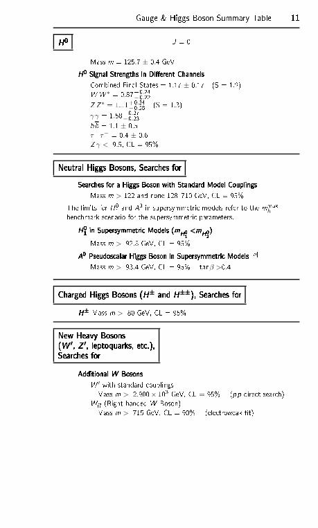
Gauge & Higgs Boson Summary Table 11111111H0H0H0H0 J = 0Mass m = 125.7 ± 0.4 GeVH0 Signal Strengths in Dierent ChannelsH0 Signal Strengths in Dierent ChannelsH0 Signal Strengths in Dierent ChannelsH0 Signal Strengths in Dierent ChannelsCombined Final States = 1.17 ± 0.17 (S = 1.2)WW ∗ = 0.87+0.24−0.22Z Z∗ = 1.11+0.34
−0.28 (S = 1.3)γ γ = 1.58+0.27
−0.23bb = 1.1 ± 0.5τ+ τ− = 0.4 ± 0.6Z γ < 9.5, CL = 95%Neutral Higgs Bosons, Sear hes forNeutral Higgs Bosons, Sear hes forNeutral Higgs Bosons, Sear hes forNeutral Higgs Bosons, Sear hes forSear hes for a Higgs Boson with Standard Model CouplingsSear hes for a Higgs Boson with Standard Model CouplingsSear hes for a Higgs Boson with Standard Model CouplingsSear hes for a Higgs Boson with Standard Model CouplingsMass m > 122 and none 128710 GeV, CL = 95%The limits for H01 and A0 in supersymmetri models refer to the mmax
hben hmark s enario for the supersymmetri parameters.H01 in Supersymmetri Models (mH01 <mH02)H01 in Supersymmetri Models (mH01 <mH02)H01 in Supersymmetri Models (mH01 <mH02)H01 in Supersymmetri Models (mH01 <mH02)Mass m > 92.8 GeV, CL = 95%A0 Pseudos alar Higgs Boson in Supersymmetri ModelsA0 Pseudos alar Higgs Boson in Supersymmetri ModelsA0 Pseudos alar Higgs Boson in Supersymmetri ModelsA0 Pseudos alar Higgs Boson in Supersymmetri Models [nMass m > 93.4 GeV, CL = 95% tanβ >0.4Charged Higgs Bosons (H± and H±±), Sear hes forCharged Higgs Bosons (H± and H±±), Sear hes forCharged Higgs Bosons (H± and H±±), Sear hes forCharged Higgs Bosons (H± and H±±), Sear hes forH±H±H±H± Mass m > 80 GeV, CL = 95%New Heavy BosonsNew Heavy BosonsNew Heavy BosonsNew Heavy Bosons(W ′, Z ′, leptoquarks, et .),(W ′, Z ′, leptoquarks, et .),(W ′, Z ′, leptoquarks, et .),(W ′, Z ′, leptoquarks, et .),Sear hes forSear hes forSear hes forSear hes forAdditional W BosonsAdditional W BosonsAdditional W BosonsAdditional W BosonsW ′ with standard ouplingsMass m > 2.900× 10³ GeV, CL = 95% (pp dire t sear h)WR (Right-handed W Boson)Mass m > 715 GeV, CL = 90% (ele troweak t)
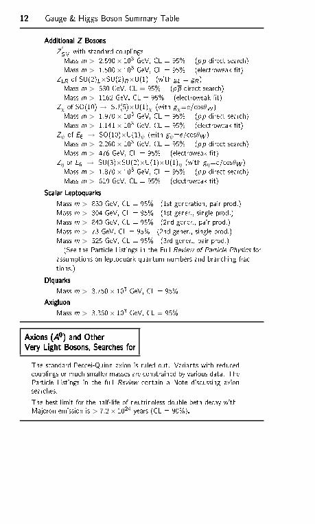
12121212 Gauge & Higgs Boson Summary TableAdditional Z BosonsAdditional Z BosonsAdditional Z BosonsAdditional Z BosonsZ ′SM with standard ouplingsMass m > 2.590× 10³ GeV, CL = 95% (pp dire t sear h)Mass m > 1.500× 10³ GeV, CL = 95% (ele troweak t)ZLR of SU(2)L×SU(2)R×U(1) (with gL = gR)Mass m > 630 GeV, CL = 95% (pp dire t sear h)Mass m > 1162 GeV, CL = 95% (ele troweak t)Zχ of SO(10) → SU(5)×U(1)χ (with gχ=e/ osθW )Mass m > 1.970× 10³ GeV, CL = 95% (pp dire t sear h)Mass m > 1.141× 10³ GeV, CL = 95% (ele troweak t)Zψ of E6 → SO(10)×U(1)ψ (with gψ=e/ osθW )Mass m > 2.260× 10³ GeV, CL = 95% (pp dire t sear h)Mass m > 476 GeV, CL = 95% (ele troweak t)Zη of E6 → SU(3)×SU(2)×U(1)×U(1)η (with gη=e/ osθW )Mass m > 1.870× 10³ GeV, CL = 95% (pp dire t sear h)Mass m > 619 GeV, CL = 95% (ele troweak t)S alar LeptoquarksS alar LeptoquarksS alar LeptoquarksS alar LeptoquarksMass m > 830 GeV, CL = 95% (1st generation, pair prod.)Mass m > 304 GeV, CL = 95% (1st gener., single prod.)Mass m > 840 GeV, CL = 95% (2nd gener., pair prod.)Mass m > 73 GeV, CL = 95% (2nd gener., single prod.)Mass m > 525 GeV, CL = 95% (3rd gener., pair prod.)(See the Parti le Listings in the Full Review of Parti le Physi s forassumptions on leptoquark quantum numbers and bran hing fra -tions.)DiquarksDiquarksDiquarksDiquarksMass m > 3.750× 10³ GeV, CL = 95%AxigluonAxigluonAxigluonAxigluonMass m > 3.360× 10³ GeV, CL = 95%Axions (A0) and OtherAxions (A0) and OtherAxions (A0) and OtherAxions (A0) and OtherVery Light Bosons, Sear hes forVery Light Bosons, Sear hes forVery Light Bosons, Sear hes forVery Light Bosons, Sear hes forThe standard Pe ei-Quinn axion is ruled out. Variants with redu ed ouplings or mu h smaller masses are onstrained by various data. TheParti le Listings in the full Review ontain a Note dis ussing axionsear hes.The best limit for the half-life of neutrinoless double beta de ay withMajoron emission is > 7.2× 1024 years (CL = 90%).
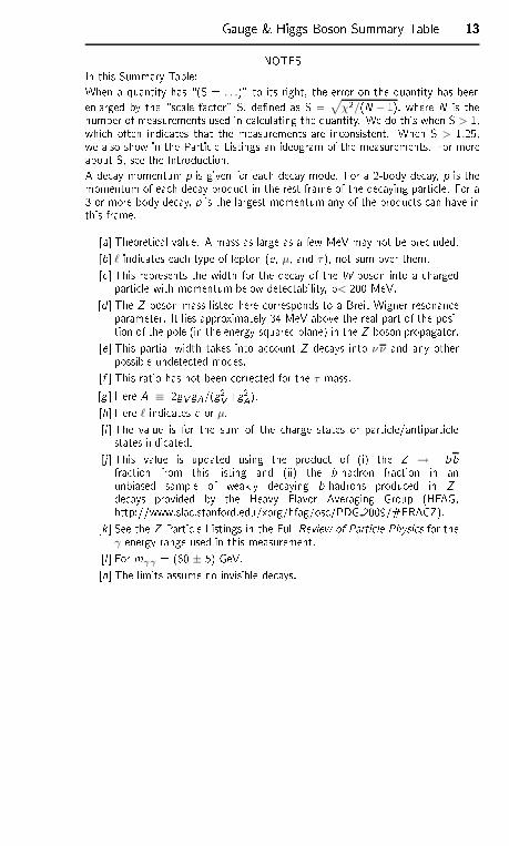
Gauge & Higgs Boson Summary Table 13131313NOTESIn this Summary Table:When a quantity has \(S = . . .)" to its right, the error on the quantity has beenenlarged by the \s ale fa tor" S, dened as S = √
χ2/(N − 1), where N is thenumber of measurements used in al ulating the quantity. We do this when S > 1,whi h often indi ates that the measurements are in onsistent. When S > 1.25,we also show in the Parti le Listings an ideogram of the measurements. For moreabout S, see the Introdu tion.A de ay momentum p is given for ea h de ay mode. For a 2-body de ay, p is themomentum of ea h de ay produ t in the rest frame of the de aying parti le. For a3-or-more-body de ay, p is the largest momentum any of the produ ts an have inthis frame.[a Theoreti al value. A mass as large as a few MeV may not be pre luded.[b ℓ indi ates ea h type of lepton (e, µ, and τ), not sum over them.[ This represents the width for the de ay of the W boson into a hargedparti le with momentum below dete tability, p< 200 MeV.[d The Z -boson mass listed here orresponds to a Breit-Wigner resonan eparameter. It lies approximately 34 MeV above the real part of the posi-tion of the pole (in the energy-squared plane) in the Z -boson propagator.[e This partial width takes into a ount Z de ays into ν ν and any otherpossible undete ted modes.[f This ratio has not been orre ted for the τ mass.[g Here A ≡ 2gV gA/(g2V+g2A).[h Here ℓ indi ates e or µ.[i The value is for the sum of the harge states or parti le/antiparti lestates indi ated.[j This value is updated using the produ t of (i) the Z → bbfra tion from this listing and (ii) the b-hadron fra tion in anunbiased sample of weakly de aying b-hadrons produ ed in Z -de ays provided by the Heavy Flavor Averaging Group (HFAG,http://www.sla .stanford.edu/xorg/hfag/os /PDG 2009/#FRACZ).[k See the Z Parti le Listings in the Full Review of Parti le Physi s for theγ energy range used in this measurement.[l For mγ γ = (60 ± 5) GeV.[n The limits assume no invisible de ays.
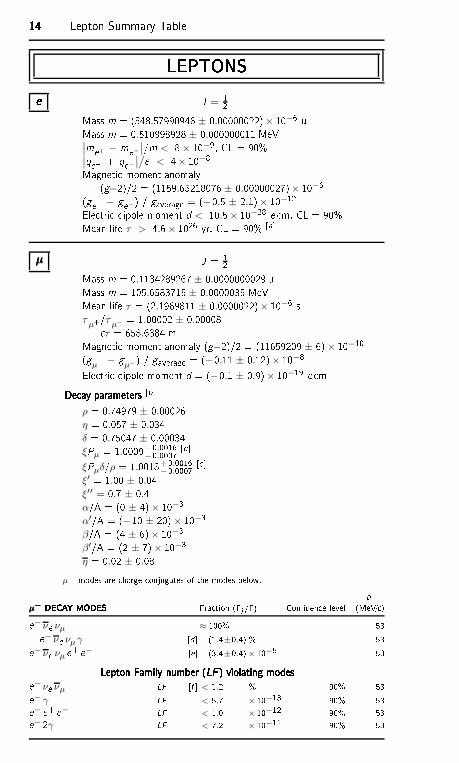
14141414 Lepton Summary TableLEPTONSLEPTONSLEPTONSLEPTONSeeee J = 12Mass m = (548.57990946 ± 0.00000022)× 10−6 uMass m = 0.510998928 ± 0.000000011 MeV∣
∣me+ − me−∣
∣/m < 8× 10⁻⁹, CL = 90%∣
∣qe+ + qe− ∣
∣
/e < 4× 10⁻⁸Magneti moment anomaly(g−2)/2 = (1159.65218076 ± 0.00000027)× 10−6(ge+ − ge−) / gaverage = (−0.5 ± 2.1)× 10−12Ele tri dipole moment d < 10.5× 10⁻²⁸ e m, CL = 90%Mean life τ > 4.6× 1026 yr, CL = 90% [aµµµµ J = 12Mass m = 0.1134289267 ± 0.0000000029 uMass m = 105.6583715 ± 0.0000035 MeVMean life τ = (2.1969811 ± 0.0000022)× 10−6 s
τµ+/τ µ− = 1.00002 ± 0.00008 τ = 658.6384 mMagneti moment anomaly (g−2)/2 = (11659209 ± 6)× 10−10(gµ+ − g
µ−) / gaverage = (−0.11 ± 0.12)× 10−8Ele tri dipole moment d = (−0.1 ± 0.9)× 10−19 e mDe ay parametersDe ay parametersDe ay parametersDe ay parameters [bρ = 0.74979 ± 0.00026η = 0.057 ± 0.034δ = 0.75047 ± 0.00034ξPµ = 1.0009+0.0016
−0.0007 [ ξPµδ/ρ = 1.0018+0.0016
−0.0007 [ ξ′ = 1.00 ± 0.04ξ′′ = 0.7 ± 0.4α/A = (0 ± 4)× 10−3α′/A = (−10 ± 20)× 10−3β/A = (4 ± 6)× 10−3β′/A = (2 ± 7)× 10−3η = 0.02 ± 0.08
µ+ modes are harge onjugates of the modes below. pµ− DECAY MODESµ− DECAY MODESµ− DECAY MODESµ− DECAY MODES Fra tion (i /) Conden e level (MeV/ )e− νe νµ ≈ 100% 53e− νe νµ γ [d (1.4±0.4) % 53e− νe νµ e+ e− [e (3.4±0.4)× 10−5 53Lepton Family number (LF ) violating modesLepton Family number (LF ) violating modesLepton Family number (LF ) violating modesLepton Family number (LF ) violating modese− νe νµ LF [f < 1.2 % 90% 53e− γ LF < 5.7 × 10⁻¹³ 90% 53e− e+ e− LF < 1.0 × 10⁻¹² 90% 53e− 2γ LF < 7.2 × 10⁻¹¹ 90% 53
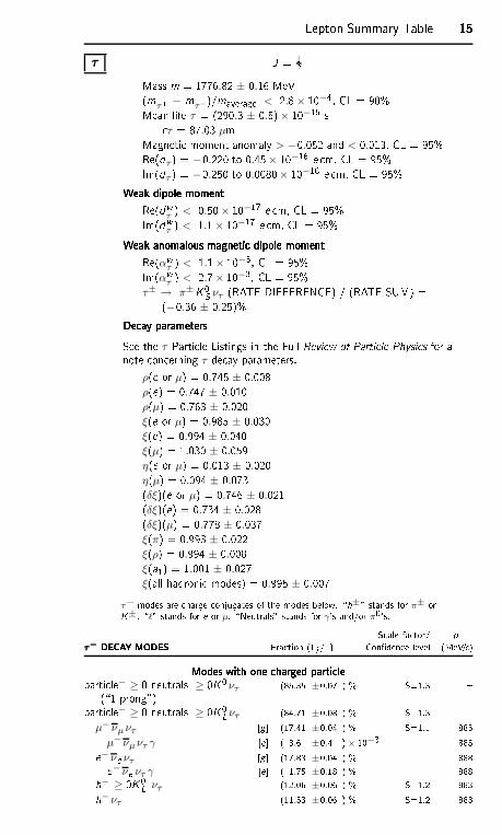
Lepton Summary Table 15151515ττττ J = 12Mass m = 1776.82 ± 0.16 MeV(mτ+ − mτ−)/maverage < 2.8× 10⁻⁴, CL = 90%Mean life τ = (290.3 ± 0.5)× 10−15 s τ = 87.03 µmMagneti moment anomaly > −0.052 and < 0.013, CL = 95%Re(dτ ) = −0.220 to 0.45× 10⁻¹⁶ e m, CL = 95%Im(dτ ) = −0.250 to 0.0080× 10⁻¹⁶ e m, CL = 95%Weak dipole momentWeak dipole momentWeak dipole momentWeak dipole momentRe(dwτ ) < 0.50× 10⁻¹⁷ e m, CL = 95%Im(dwτ ) < 1.1× 10⁻¹⁷ e m, CL = 95%Weak anomalous magneti dipole momentWeak anomalous magneti dipole momentWeak anomalous magneti dipole momentWeak anomalous magneti dipole momentRe(αw
τ ) < 1.1× 10⁻³, CL = 95%Im(αwτ ) < 2.7× 10⁻³, CL = 95%
τ± → π±K0S ντ (RATE DIFFERENCE) / (RATE SUM) =(−0.36 ± 0.25)%De ay parametersDe ay parametersDe ay parametersDe ay parametersSee the τ Parti le Listings in the Full Review of Parti le Physi s for anote on erning τ -de ay parameters.ρ(e or µ) = 0.745 ± 0.008ρ(e) = 0.747 ± 0.010ρ(µ) = 0.763 ± 0.020ξ(e or µ) = 0.985 ± 0.030ξ(e) = 0.994 ± 0.040ξ(µ) = 1.030 ± 0.059η(e or µ) = 0.013 ± 0.020η(µ) = 0.094 ± 0.073(δξ)(e or µ) = 0.746 ± 0.021(δξ)(e) = 0.734 ± 0.028(δξ)(µ) = 0.778 ± 0.037ξ(π) = 0.993 ± 0.022ξ(ρ) = 0.994 ± 0.008ξ(a1) = 1.001 ± 0.027ξ(all hadroni modes) = 0.995 ± 0.007
τ+ modes are harge onjugates of the modes below. \h±" stands for π± orK±. \ℓ" stands for e or µ. \Neutrals" stands for γ's and/or π0's.S ale fa tor/ pτ− DECAY MODESτ− DECAY MODESτ− DECAY MODESτ− DECAY MODES Fra tion (i /) Conden e level (MeV/ )Modes with one harged parti leModes with one harged parti leModes with one harged parti leModes with one harged parti leparti le− ≥ 0 neutrals ≥ 0K 0ντ(\1-prong") (85.35 ±0.07 ) % S=1.3 parti le− ≥ 0 neutrals ≥ 0K 0Lντ (84.71 ±0.08 ) % S=1.3
µ−νµ ντ [g (17.41 ±0.04 ) % S=1.1 885µ−νµ ντ γ [e ( 3.6 ±0.4 )× 10−3 885e− νe ντ [g (17.83 ±0.04 ) % 888e− νe ντ γ [e ( 1.75 ±0.18 ) % 888h− ≥ 0K0L ντ (12.06 ±0.06 ) % S=1.2 883h−ντ (11.53 ±0.06 ) % S=1.2 883
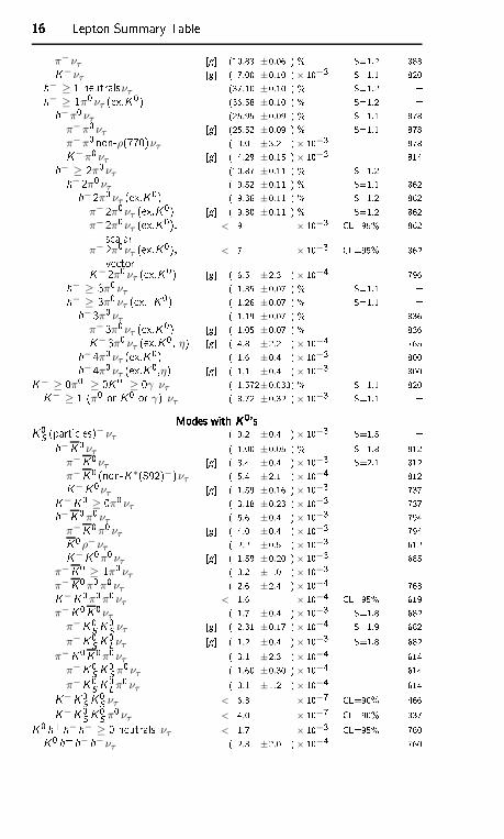
16161616 Lepton Summary Tableπ− ντ [g (10.83 ±0.06 ) % S=1.2 883K−ντ [g ( 7.00 ±0.10 )× 10−3 S=1.1 820h− ≥ 1 neutralsντ (37.10 ±0.10 ) % S=1.2 h− ≥ 1π0 ντ (ex.K0) (36.58 ±0.10 ) % S=1.2 h−π0 ντ (25.95 ±0.09 ) % S=1.1 878
π−π0 ντ [g (25.52 ±0.09 ) % S=1.1 878π−π0 non-ρ(770)ντ ( 3.0 ±3.2 )× 10−3 878K−π0 ντ [g ( 4.29 ±0.15 )× 10−3 814h− ≥ 2π0 ντ (10.87 ±0.11 ) % S=1.2 h−2π0 ντ ( 9.52 ±0.11 ) % S=1.1 862h−2π0 ντ (ex.K0) ( 9.36 ±0.11 ) % S=1.2 862
π− 2π0ντ (ex.K0) [g ( 9.30 ±0.11 ) % S=1.2 862π− 2π0ντ (ex.K0),s alar < 9 × 10⁻³ CL=95% 862π− 2π0ντ (ex.K0),ve tor < 7 × 10⁻³ CL=95% 862K−2π0 ντ (ex.K0) [g ( 6.5 ±2.3 )× 10−4 796h− ≥ 3π0 ντ ( 1.35 ±0.07 ) % S=1.1 h− ≥ 3π0 ντ (ex. K0) ( 1.26 ±0.07 ) % S=1.1 h−3π0 ντ ( 1.19 ±0.07 ) % 836π− 3π0ντ (ex.K0) [g ( 1.05 ±0.07 ) % 836K−3π0 ντ (ex.K0, η) [g ( 4.8 ±2.2 )× 10−4 765h−4π0 ντ (ex.K0) ( 1.6 ±0.4 )× 10−3 800h−4π0 ντ (ex.K0,η) [g ( 1.1 ±0.4 )× 10−3 800K− ≥ 0π0 ≥ 0K0 ≥ 0γ ντ ( 1.572±0.033) % S=1.1 820K− ≥ 1 (π0 or K0 or γ) ντ ( 8.72 ±0.32 )× 10−3 S=1.1 Modes with K0'sModes with K0'sModes with K0'sModes with K0'sK0S (parti les)− ντ ( 9.2 ±0.4 )× 10−3 S=1.5 h−K0 ντ ( 1.00 ±0.05 ) % S=1.8 812
π−K0 ντ [g ( 8.4 ±0.4 )× 10−3 S=2.1 812π−K0 (non-K∗(892)−)ντ ( 5.4 ±2.1 )× 10−4 812K−K0ντ [g ( 1.59 ±0.16 )× 10−3 737K−K0 ≥ 0π0 ντ ( 3.18 ±0.23 )× 10−3 737h−K0π0 ντ ( 5.6 ±0.4 )× 10−3 794π−K0π0 ντ [g ( 4.0 ±0.4 )× 10−3 794K0ρ− ντ ( 2.2 ±0.5 )× 10−3 612K−K0π0 ντ [g ( 1.59 ±0.20 )× 10−3 685
π−K0 ≥ 1π0 ντ ( 3.2 ±1.0 )× 10−3 π−K0π0π0 ντ ( 2.6 ±2.4 )× 10−4 763K−K0π0π0 ντ < 1.6 × 10⁻⁴ CL=95% 619π−K0K0ντ ( 1.7 ±0.4 )× 10−3 S=1.8 682
π−K0S K0S ντ [g ( 2.31 ±0.17 )× 10−4 S=1.9 682π−K0S K0Lντ [g ( 1.2 ±0.4 )× 10−3 S=1.8 682
π−K0K0π0 ντ ( 3.1 ±2.3 )× 10−4 614π−K0S K0S π0 ντ ( 1.60 ±0.30 )× 10−4 614π−K0S K0Lπ0 ντ ( 3.1 ±1.2 )× 10−4 614K−K0S K0S ντ < 6.3 × 10⁻⁷ CL=90% 466K−K0S K0S π0 ντ < 4.0 × 10⁻⁷ CL=90% 337K0h+ h−h− ≥ 0 neutrals ντ < 1.7 × 10⁻³ CL=95% 760K0h+ h−h−ντ ( 2.3 ±2.0 )× 10−4 760
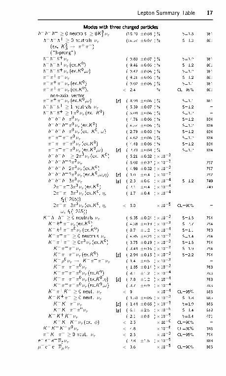
Lepton Summary Table 17171717Modes with three harged parti lesModes with three harged parti lesModes with three harged parti lesModes with three harged parti lesh−h− h+ ≥ 0 neutrals ≥ 0K 0Lντ (15.20 ±0.08 ) % S=1.3 861h− h−h+ ≥ 0 neutrals ντ(ex. K0S → π+π−)(\3-prong") (14.57 ±0.07 ) % S=1.3 861h−h− h+ντ ( 9.80 ±0.07 ) % S=1.2 861h−h− h+ντ (ex.K0) ( 9.46 ±0.06 ) % S=1.2 861h−h− h+ντ (ex.K0,ω) ( 9.42 ±0.06 ) % S=1.2 861π−π+π− ντ ( 9.31 ±0.06 ) % S=1.2 861π−π+π− ντ (ex.K0) ( 9.02 ±0.06 ) % S=1.1 861π−π+π− ντ (ex.K0),non-axial ve tor < 2.4 % CL=95% 861π−π+π− ντ (ex.K0,ω) [g ( 8.99 ±0.06 ) % S=1.1 861h−h− h+ ≥ 1 neutrals ντ ( 5.39 ±0.07 ) % S=1.2 h−h− h+ ≥ 1π0 ντ (ex. K0) ( 5.09 ±0.06 ) % S=1.2 h−h− h+π0 ντ ( 4.76 ±0.06 ) % S=1.2 834h−h− h+π0 ντ (ex.K0) ( 4.57 ±0.06 ) % S=1.2 834h−h− h+π0 ντ (ex. K0, ω) ( 2.79 ±0.08 ) % S=1.2 834
π−π+π−π0 ντ ( 4.62 ±0.06 ) % S=1.2 834π−π+π−π0 ντ (ex.K0) ( 4.48 ±0.06 ) % S=1.2 834π−π+π−π0 ντ (ex.K0,ω) [g ( 2.70 ±0.08 ) % S=1.2 834h−h− h+ ≥ 2π0 ντ (ex. K0) ( 5.21 ±0.32 )× 10−3 h−h− h+2π0 ντ ( 5.08 ±0.32 )× 10−3 797h−h− h+2π0 ντ (ex.K0) ( 4.98 ±0.32 )× 10−3 797h−h− h+2π0 ντ (ex.K0,ω,η) [g ( 1.0 ±0.4 )× 10−3 797h−h− h+3π0 ντ [g ( 2.3 ±0.6 )× 10−4 S=1.2 7492π−π+ 3π0ντ (ex.K0) ( 2.1 ±0.4 )× 10−4 7492π−π+ 3π0ντ (ex.K0, η,f1(1285)) ( 1.7 ±0.4 )× 10−4 2π−π+ 3π0ντ (ex.K0, η,
ω, f1(1285)) < 5.8 × 10⁻⁵ CL=90% K−h+h− ≥ 0 neutrals ντ ( 6.35 ±0.24 )× 10−3 S=1.5 794K−h+π− ντ (ex.K0) ( 4.38 ±0.19 )× 10−3 S=2.7 794K−h+π−π0 ντ (ex.K0) ( 8.7 ±1.2 )× 10−4 S=1.1 763K−π+π− ≥ 0 neutrals ντ ( 4.85 ±0.21 )× 10−3 S=1.4 794K−π+π− ≥ 0π0 ντ (ex.K0) ( 3.75 ±0.19 )× 10−3 S=1.5 794K−π+π−ντ ( 3.49 ±0.16 )× 10−3 S=1.9 794K−π+π−ντ (ex.K0) [g ( 2.94 ±0.15 )× 10−3 S=2.2 794K−ρ0 ντ → K−π+π−ντ ( 1.4 ±0.5 )× 10−3 K−π+π−π0 ντ ( 1.35 ±0.14 )× 10−3 763K−π+π−π0 ντ (ex.K0) ( 8.1 ±1.2 )× 10−4 763K−π+π−π0 ντ (ex.K0,η) [g ( 7.8 ±1.2 )× 10−4 763K−π+π−π0 ντ (ex.K0,ω) ( 3.7 ±0.9 )× 10−4 763K−π+K− ≥ 0 neut. ντ < 9 × 10⁻⁴ CL=95% 685K−K+π− ≥ 0 neut. ντ ( 1.50 ±0.06 )× 10−3 S=1.8 685K−K+π− ντ [g ( 1.44 ±0.05 )× 10−3 S=1.9 685K−K+π−π0 ντ [g ( 6.1 ±2.5 )× 10−5 S=1.4 618K−K+K−ντ ( 2.1 ±0.8 )× 10−5 S=5.4 471K−K+K−ντ (ex. φ) < 2.5 × 10⁻⁶ CL=90% K−K+K−π0 ντ < 4.8 × 10⁻⁶ CL=90% 345π−K+π− ≥ 0 neut. ντ < 2.5 × 10⁻³ CL=95% 794e− e− e+ νe ντ ( 2.8 ±1.5 )× 10−5 888
µ− e− e+νµ ντ < 3.6 × 10⁻⁵ CL=90% 885
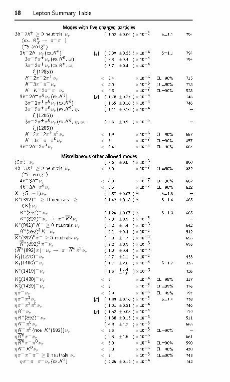
18181818 Lepton Summary TableModes with ve harged parti lesModes with ve harged parti lesModes with ve harged parti lesModes with ve harged parti les3h−2h+ ≥ 0 neutrals ντ(ex. K0S → π−π+)(\5-prong") ( 1.02 ±0.04 )× 10−3 S=1.1 7943h−2h+ντ (ex.K0) [g ( 8.39 ±0.35 )× 10−4 S=1.1 7943π−2π+ντ (ex.K0, ω) ( 8.3 ±0.4 )× 10−4 7943π−2π+ντ (ex.K0, ω,f1(1285)) ( 7.7 ±0.4 )× 10−4 K−2π−2π+ντ < 2.4 × 10⁻⁶ CL=90% 715K+3π−π+ ντ < 5.0 × 10⁻⁶ CL=90% 715K+K−2π−π+ ντ < 4.5 × 10⁻⁷ CL=90% 5283h−2h+π0 ντ (ex.K0) [g ( 1.78 ±0.27 )× 10−4 7463π−2π+π0 ντ (ex.K0) ( 1.65 ±0.10 )× 10−4 7463π−2π+π0 ντ (ex.K0, η,f1(1285)) ( 1.11 ±0.10 )× 10−4 3π−2π+π0 ντ (ex.K0, η, ω,f1(1285)) ( 3.6 ±0.9 )× 10−5 K−2π−2π+π0 ντ < 1.9 × 10⁻⁶ CL=90% 657K+3π−π+π0 ντ < 8 × 10⁻⁷ CL=90% 6573h−2h+2π0ντ < 3.4 × 10⁻⁶ CL=90% 687Mis ellaneous other allowed modesMis ellaneous other allowed modesMis ellaneous other allowed modesMis ellaneous other allowed modes(5π )− ντ ( 7.6 ±0.5 )× 10−3 8004h−3h+ ≥ 0 neutrals ντ(\7-prong") < 3.0 × 10⁻⁷ CL=90% 6824h−3h+ντ < 4.3 × 10⁻⁷ CL=90% 6824h−3h+π0 ντ < 2.5 × 10⁻⁷ CL=90% 612X− (S=−1)ντ ( 2.87 ±0.07 ) % S=1.3 K∗(892)− ≥ 0 neutrals ≥0K0Lντ
( 1.42 ±0.18 ) % S=1.4 665K∗(892)− ντ ( 1.20 ±0.07 ) % S=1.8 665K∗(892)− ντ → π−K0 ντ ( 7.9 ±0.5 )× 10−3 K∗(892)0K− ≥ 0 neutrals ντ ( 3.2 ±1.4 )× 10−3 542K∗(892)0K−ντ ( 2.1 ±0.4 )× 10−3 542K∗(892)0π− ≥ 0 neutrals ντ ( 3.8 ±1.7 )× 10−3 655K∗(892)0π− ντ ( 2.2 ±0.5 )× 10−3 655(K∗(892)π )− ντ → π−K0π0 ντ ( 1.0 ±0.4 )× 10−3 K1(1270)−ντ ( 4.7 ±1.1 )× 10−3 433K1(1400)−ντ ( 1.7 ±2.6 )× 10−3 S=1.7 335K∗(1410)−ντ ( 1.5 +1.4−1.0 )× 10−3 326K∗0(1430)−ντ < 5 × 10⁻⁴ CL=95% 317K∗2(1430)−ντ < 3 × 10⁻³ CL=95% 316
ηπ− ντ < 9.9 × 10⁻⁵ CL=95% 797ηπ−π0 ντ [g ( 1.39 ±0.10 )× 10−3 S=1.4 778ηπ−π0π0 ντ ( 1.81 ±0.31 )× 10−4 746ηK− ντ [g ( 1.52 ±0.08 )× 10−4 719ηK∗(892)−ντ ( 1.38 ±0.15 )× 10−4 511ηK−π0 ντ ( 4.8 ±1.2 )× 10−5 665ηK−π0 (non-K∗(892))ντ < 3.5 × 10⁻⁵ CL=90% ηK0π− ντ ( 9.3 ±1.5 )× 10−5 661ηK0π−π0 ντ < 5.0 × 10⁻⁵ CL=90% 590ηK−K0ντ < 9.0 × 10⁻⁶ CL=90% 430ηπ+π−π− ≥ 0 neutrals ντ < 3 × 10⁻³ CL=90% 743
ηπ−π+π− ντ (ex.K0) ( 2.25 ±0.13 )× 10−4 743
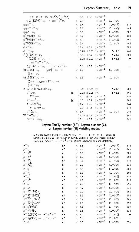
Lepton Summary Table 19191919ηπ−π+π− ντ (ex.K0,f1(1285)) ( 9.9 ±1.6 )× 10−5
ηa1(1260)−ντ → ηπ− ρ0 ντ < 3.9 × 10⁻⁴ CL=90% ηηπ− ντ < 7.4 × 10⁻⁶ CL=90% 637ηηπ−π0 ντ < 2.0 × 10⁻⁴ CL=95% 559ηηK− ντ < 3.0 × 10⁻⁶ CL=90% 382η′(958)π− ντ < 4.0 × 10⁻⁶ CL=90% 620η′(958)π−π0 ντ < 1.2 × 10⁻⁵ CL=90% 591η′(958)K−ντ < 2.4 × 10⁻⁶ CL=90% 495φπ− ντ ( 3.4 ±0.6 )× 10−5 585φK− ντ ( 3.70 ±0.33 )× 10−5 S=1.3 445f1(1285)π−ντ ( 3.9 ±0.5 )× 10−4 S=1.9 408f1(1285)π−ντ →
ηπ−π+π− ντ
( 1.18 ±0.07 )× 10−4 S=1.3 f1(1285)π−ντ → 3π−2π+ντ ( 5.2 ±0.5 )× 10−5 π(1300)−ντ → (ρπ)− ντ →(3π)− ντ
< 1.0 × 10⁻⁴ CL=90% π(1300)−ντ →((ππ)S−wave π)− ντ →(3π)− ντ
< 1.9 × 10⁻⁴ CL=90% h−ω ≥ 0 neutrals ντ ( 2.41 ±0.09 ) % S=1.2 708h−ωντ [g ( 2.00 ±0.08 ) % S=1.3 708K−ωντ ( 4.1 ±0.9 )× 10−4 610h−ωπ0 ντ [g ( 4.1 ±0.4 )× 10−3 684h−ω2π0 ντ ( 1.4 ±0.5 )× 10−4 644π−ω2π0ντ ( 7.3 ±1.7 )× 10−5 644h−2ωντ < 5.4 × 10⁻⁷ CL=90% 2492h−h+ωντ ( 1.20 ±0.22 )× 10−4 6412π−π+ωντ ( 8.4 ±0.7 )× 10−5 641Lepton Family number (LF ), Lepton number (L),Lepton Family number (LF ), Lepton number (L),Lepton Family number (LF ), Lepton number (L),Lepton Family number (LF ), Lepton number (L),or Baryon number (B) violating modesor Baryon number (B) violating modesor Baryon number (B) violating modesor Baryon number (B) violating modesL means lepton number violation (e.g. τ− → e+π−π−). Following ommon usage, LF means lepton family violation and not lepton numberviolation (e.g. τ− → e−π+π−). B means baryon number violation.e− γ LF < 3.3 × 10⁻⁸ CL=90% 888
µ−γ LF < 4.4 × 10⁻⁸ CL=90% 885e−π0 LF < 8.0 × 10⁻⁸ CL=90% 883µ−π0 LF < 1.1 × 10⁻⁷ CL=90% 880e−K0S LF < 2.6 × 10⁻⁸ CL=90% 819µ−K0S LF < 2.3 × 10⁻⁸ CL=90% 815e− η LF < 9.2 × 10⁻⁸ CL=90% 804µ−η LF < 6.5 × 10⁻⁸ CL=90% 800e− ρ0 LF < 1.8 × 10⁻⁸ CL=90% 719µ−ρ0 LF < 1.2 × 10⁻⁸ CL=90% 715e−ω LF < 4.8 × 10⁻⁸ CL=90% 716µ−ω LF < 4.7 × 10⁻⁸ CL=90% 711e−K∗(892)0 LF < 3.2 × 10⁻⁸ CL=90% 665µ−K∗(892)0 LF < 5.9 × 10⁻⁸ CL=90% 659e−K∗(892)0 LF < 3.4 × 10⁻⁸ CL=90% 665µ−K∗(892)0 LF < 7.0 × 10⁻⁸ CL=90% 659e− η′(958) LF < 1.6 × 10⁻⁷ CL=90% 630µ−η′(958) LF < 1.3 × 10⁻⁷ CL=90% 625e− f0(980) → e−π+π− LF < 3.2 × 10⁻⁸ CL=90% µ− f0(980) → µ−π+π− LF < 3.4 × 10⁻⁸ CL=90% e−φ LF < 3.1 × 10⁻⁸ CL=90% 596
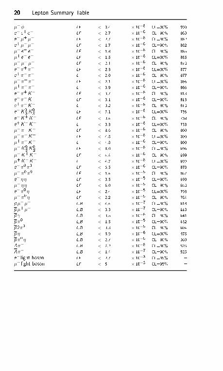
20202020 Lepton Summary Tableµ−φ LF < 8.4 × 10⁻⁸ CL=90% 590e− e+ e− LF < 2.7 × 10⁻⁸ CL=90% 888e−µ+µ− LF < 2.7 × 10⁻⁸ CL=90% 882e+µ−µ− LF < 1.7 × 10⁻⁸ CL=90% 882µ− e+ e− LF < 1.8 × 10⁻⁸ CL=90% 885µ+ e− e− LF < 1.5 × 10⁻⁸ CL=90% 885µ−µ+µ− LF < 2.1 × 10⁻⁸ CL=90% 873e−π+π− LF < 2.3 × 10⁻⁸ CL=90% 877e+π−π− L < 2.0 × 10⁻⁸ CL=90% 877µ−π+π− LF < 2.1 × 10⁻⁸ CL=90% 866µ+π−π− L < 3.9 × 10⁻⁸ CL=90% 866e−π+K− LF < 3.7 × 10⁻⁸ CL=90% 813e−π−K+ LF < 3.1 × 10⁻⁸ CL=90% 813e+π−K− L < 3.2 × 10⁻⁸ CL=90% 813e−K0S K0S LF < 7.1 × 10⁻⁸ CL=90% 736e−K+K− LF < 3.4 × 10⁻⁸ CL=90% 738e+K−K− L < 3.3 × 10⁻⁸ CL=90% 738µ−π+K− LF < 8.6 × 10⁻⁸ CL=90% 800µ−π−K+ LF < 4.5 × 10⁻⁸ CL=90% 800µ+π−K− L < 4.8 × 10⁻⁸ CL=90% 800µ−K0S K0S LF < 8.0 × 10⁻⁸ CL=90% 696µ−K+K− LF < 4.4 × 10⁻⁸ CL=90% 699µ+K−K− L < 4.7 × 10⁻⁸ CL=90% 699e−π0π0 LF < 6.5 × 10⁻⁶ CL=90% 878µ−π0π0 LF < 1.4 × 10⁻⁵ CL=90% 867e− ηη LF < 3.5 × 10⁻⁵ CL=90% 699µ−ηη LF < 6.0 × 10⁻⁵ CL=90% 653e−π0 η LF < 2.4 × 10⁻⁵ CL=90% 798µ−π0 η LF < 2.2 × 10⁻⁵ CL=90% 784pµ−µ− L,B < 4.4 × 10⁻⁷ CL=90% 618pµ+µ− L,B < 3.3 × 10⁻⁷ CL=90% 618pγ L,B < 3.5 × 10⁻⁶ CL=90% 641pπ0 L,B < 1.5 × 10⁻⁵ CL=90% 632p2π0 L,B < 3.3 × 10⁻⁵ CL=90% 604pη L,B < 8.9 × 10⁻⁶ CL=90% 475pπ0 η L,B < 2.7 × 10⁻⁵ CL=90% 360π− L,B < 7.2 × 10⁻⁸ CL=90% 525π− L,B < 1.4 × 10⁻⁷ CL=90% 525e− light boson LF < 2.7 × 10⁻³ CL=95% µ− light boson LF < 5 × 10⁻³ CL=95%
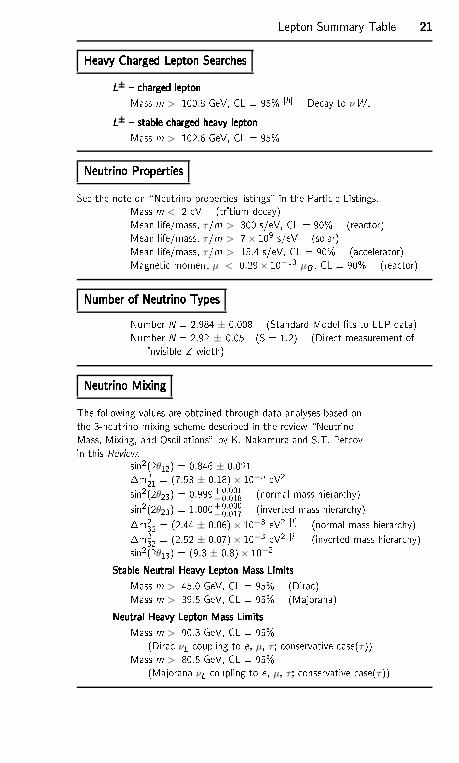
Lepton Summary Table 21212121Heavy Charged Lepton Sear hesHeavy Charged Lepton Sear hesHeavy Charged Lepton Sear hesHeavy Charged Lepton Sear hesL± harged leptonL± harged leptonL± harged leptonL± harged leptonMass m > 100.8 GeV, CL = 95% [h De ay to νW .L± stable harged heavy leptonL± stable harged heavy leptonL± stable harged heavy leptonL± stable harged heavy leptonMass m > 102.6 GeV, CL = 95%Neutrino PropertiesNeutrino PropertiesNeutrino PropertiesNeutrino PropertiesSee the note on \Neutrino properties listings" in the Parti le Listings.Mass m < 2 eV (tritium de ay)Mean life/mass, τ/m > 300 s/eV, CL = 90% (rea tor)Mean life/mass, τ/m > 7× 10⁹ s/eV (solar)Mean life/mass, τ/m > 15.4 s/eV, CL = 90% (a elerator)Magneti moment µ < 0.29× 10⁻¹⁰ µB , CL = 90% (rea tor)Number of Neutrino TypesNumber of Neutrino TypesNumber of Neutrino TypesNumber of Neutrino TypesNumber N = 2.984 ± 0.008 (Standard Model ts to LEP data)Number N = 2.92 ± 0.05 (S = 1.2) (Dire t measurement ofinvisible Z width)Neutrino MixingNeutrino MixingNeutrino MixingNeutrino MixingThe following values are obtained through data analyses based onthe 3-neutrino mixing s heme des ribed in the review \NeutrinoMass, Mixing, and Os illations" by K. Nakamura and S.T. Pet ovin this Review.sin2(2θ12) = 0.846 ± 0.021m221 = (7.53 ± 0.18)× 10−5 eV2sin2(2θ23) = 0.999+0.001−0.018 (normal mass hierar hy)sin2(2θ23) = 1.000+0.000−0.017 (inverted mass hierar hy)m232 = (2.44 ± 0.06)× 10−3 eV2 [i (normal mass hierar hy)m232 = (2.52 ± 0.07)× 10−3 eV2 [i (inverted mass hierar hy)sin2(2θ13) = (9.3 ± 0.8)× 10−2Stable Neutral Heavy Lepton Mass LimitsStable Neutral Heavy Lepton Mass LimitsStable Neutral Heavy Lepton Mass LimitsStable Neutral Heavy Lepton Mass LimitsMass m > 45.0 GeV, CL = 95% (Dira )Mass m > 39.5 GeV, CL = 95% (Majorana)Neutral Heavy Lepton Mass LimitsNeutral Heavy Lepton Mass LimitsNeutral Heavy Lepton Mass LimitsNeutral Heavy Lepton Mass LimitsMass m > 90.3 GeV, CL = 95%(Dira νL oupling to e, µ, τ ; onservative ase(τ))Mass m > 80.5 GeV, CL = 95%(Majorana νL oupling to e, µ, τ ; onservative ase(τ))
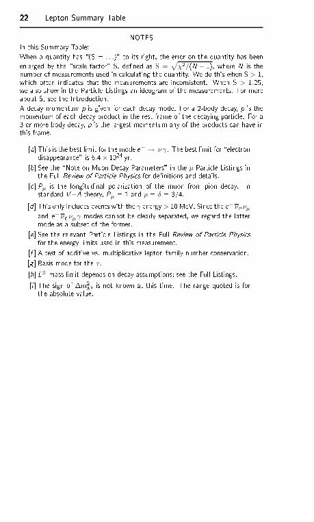
22222222 Lepton Summary Table NOTESIn this Summary Table:When a quantity has \(S = . . .)" to its right, the error on the quantity has beenenlarged by the \s ale fa tor" S, dened as S = √
χ2/(N − 1), where N is thenumber of measurements used in al ulating the quantity. We do this when S > 1,whi h often indi ates that the measurements are in onsistent. When S > 1.25,we also show in the Parti le Listings an ideogram of the measurements. For moreabout S, see the Introdu tion.A de ay momentum p is given for ea h de ay mode. For a 2-body de ay, p is themomentum of ea h de ay produ t in the rest frame of the de aying parti le. For a3-or-more-body de ay, p is the largest momentum any of the produ ts an have inthis frame.[a This is the best limit for the mode e− → ν γ. The best limit for \ele trondisappearan e" is 6.4× 1024 yr.[b See the \Note on Muon De ay Parameters" in the µ Parti le Listings inthe Full Review of Parti le Physi s for denitions and details.[ Pµ is the longitudinal polarization of the muon from pion de ay. Instandard V−A theory, Pµ = 1 and ρ = δ = 3/4.[d This only in ludes events with the γ energy > 10 MeV. Sin e the e−νe νµand e− νe νµ γ modes annot be learly separated, we regard the lattermode as a subset of the former.[e See the relevant Parti le Listings in the Full Review of Parti le Physi sfor the energy limits used in this measurement.[f A test of additive vs. multipli ative lepton family number onservation.[g Basis mode for the τ .[h L± mass limit depends on de ay assumptions; see the Full Listings.[i The sign of m232 is not known at this time. The range quoted is forthe absolute value.
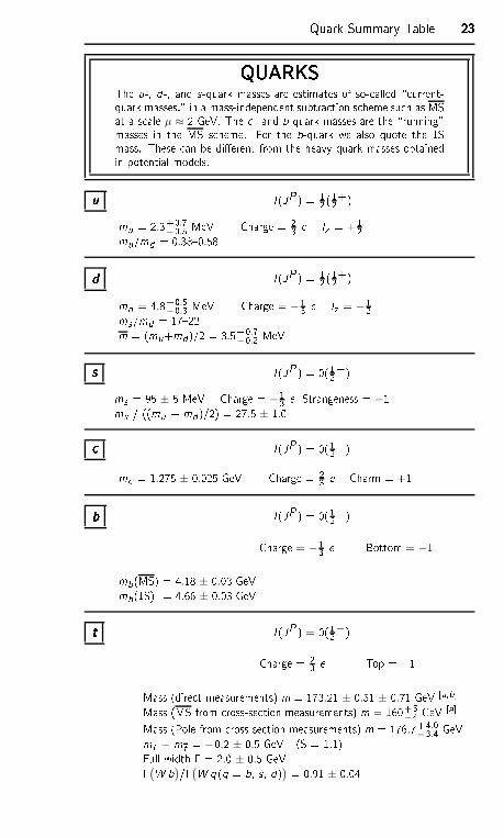
Quark Summary Table 23232323QUARKSQUARKSQUARKSQUARKSThe u-, d-, and s-quark masses are estimates of so- alled \ urrent-quark masses," in a mass-independent subtra tion s heme su h as MSat a s ale µ ≈ 2 GeV. The - and b-quark masses are the \running"masses in the MS s heme. For the b-quark we also quote the 1Smass. These an be dierent from the heavy quark masses obtainedin potential models.uuuu I (JP ) = 12 (12+)mu = 2.3+0.7−0.5 MeV Charge = 23 e Iz = +12mu/md = 0.380.58dddd I (JP ) = 12 (12+)md = 4.8+0.5−0.3 MeV Charge = −13 e Iz = −12ms/md = 1722m = (mu+md)/2 = 3.5+0.7
−0.2 MeVssss I (JP ) = 0(12+)ms = 95 ± 5 MeV Charge = − 13 e Strangeness = −1ms / ((mu + md )/2) = 27.5 ± 1.0 I (JP ) = 0(12+)m = 1.275 ± 0.025 GeV Charge = 23 e Charm = +1bbbb I (JP ) = 0(12+)Charge = −13 e Bottom = −1mb(MS) = 4.18 ± 0.03 GeVmb(1S) = 4.66 ± 0.03 GeVtttt I (JP ) = 0(12+)Charge = 23 e Top = +1Mass (dire t measurements) m = 173.21 ± 0.51 ± 0.71 GeV [a,bMass (MS from ross-se tion measurements) m = 160+5−4 GeV [aMass (Pole from ross-se tion measurements) m = 176.7+4.0
−3.4 GeVmt − mt = −0.2 ± 0.5 GeV (S = 1.1)Full width = 2.0 ± 0.5 GeV(W b)/(W q (q = b, s , d)) = 0.91 ± 0.04
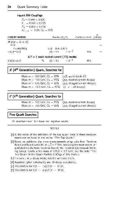
24242424 Quark Summary Tablet-quark EW Couplingst-quark EW Couplingst-quark EW Couplingst-quark EW CouplingsF0 = 0.690 ± 0.030F− = 0.314 ± 0.025F+ = 0.008 ± 0.016FV +A < 0.29, CL = 95% pt DECAY MODESt DECAY MODESt DECAY MODESt DECAY MODES Fra tion (i /) Conden e level (MeV/ )W q (q = b, s , d) W b ℓνℓ anything [ ,d (9.4±2.4) %
γ q (q=u, ) [e < 5.9 × 10⁻³ 95% T = 1 weak neutral urrent (T1) modesT = 1 weak neutral urrent (T1) modesT = 1 weak neutral urrent (T1) modesT = 1 weak neutral urrent (T1) modesZ q (q=u, ) T1 [f < 2.1 × 10⁻³ 95% b′ (4th Generation) Quark, Sear hes forb′ (4th Generation) Quark, Sear hes forb′ (4th Generation) Quark, Sear hes forb′ (4th Generation) Quark, Sear hes forMass m > 190 GeV, CL = 95% (pp, quasi-stable b′)Mass m > 400 GeV, CL = 95% (pp, neutral- urrent de ays)Mass m > 675 GeV, CL = 95% (pp, harged- urrent de ays)Mass m > 46.0 GeV, CL = 95% (e+ e−, all de ays)t ′ (4th Generation) Quark, Sear hes fort ′ (4th Generation) Quark, Sear hes fort ′ (4th Generation) Quark, Sear hes fort ′ (4th Generation) Quark, Sear hes forMass m > 782 GeV, CL = 95% (pp, neutral- urrent de ays)Mass m > 700 GeV, CL = 95% (pp, harged- urrent de ays)Free Quark Sear hesFree Quark Sear hesFree Quark Sear hesFree Quark Sear hesAll sear hes sin e 1977 have had negative results.NOTES[a A dis ussion of the denition of the top quark mass in these measure-ments an be found in the review \The Top Quark."[b Based on published top mass measurements using data from TevatronRun-I and Run-II and LHC at √s = 7 TeV. In luding the most re ent un-published results from Tevatron Run-II, the Tevatron Ele troweak Work-ing Group reports a top mass of 173.2 ± 0.9 GeV. See the note \TheTop Quark' in the Quark Parti le Listings of this Review.[ ℓ means e or µ de ay mode, not the sum over them.[d Assumes lepton universality and W -de ay a eptan e.[e This limit is for (t → γ q)/(t → W b).[f This limit is for (t → Z q)/(t → W b).
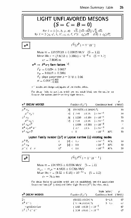
Meson Summary Table 25252525LIGHT UNFLAVORED MESONSLIGHT UNFLAVORED MESONSLIGHT UNFLAVORED MESONSLIGHT UNFLAVORED MESONS(S = C = B = 0)(S = C = B = 0)(S = C = B = 0)(S = C = B = 0)For I = 1 (π, b, ρ, a): ud , (uu−dd)/√2, du;for I = 0 (η, η′, h, h′, ω, φ, f , f ′): 1(uu + d d) + 2(s s)π±π±π±π± IG (JP ) = 1−(0−)Mass m = 139.57018 ± 0.00035 MeV (S = 1.2)Mean life τ = (2.6033 ± 0.0005)× 10−8 s (S = 1.2) τ = 7.8045 m
π± → ℓ±ν γ form fa torsπ± → ℓ±ν γ form fa torsπ± → ℓ±ν γ form fa torsπ± → ℓ±ν γ form fa tors [aFV = 0.0254 ± 0.0017FA = 0.0119 ± 0.0001FV slope parameter a = 0.10 ± 0.06R = 0.059+0.009−0.008
π− modes are harge onjugates of the modes below.For de ay limits to parti les whi h are not established, see the se tion onSear hes for Axions and Other Very Light Bosons. pπ+ DECAY MODESπ+ DECAY MODESπ+ DECAY MODESπ+ DECAY MODES Fra tion (i /) Conden e level (MeV/ )µ+νµ [b (99.98770±0.00004) % 30
µ+νµ γ [ ( 2.00 ±0.25 )× 10−4 30e+ νe [b ( 1.230 ±0.004 )× 10−4 70e+ νe γ [ ( 7.39 ±0.05 )× 10−7 70e+ νe π0 ( 1.036 ±0.006 )× 10−8 4e+ νe e+ e− ( 3.2 ±0.5 )× 10−9 70e+ νe ν ν < 5 × 10⁻⁶ 90% 70Lepton Family number (LF) or Lepton number (L) violating modesLepton Family number (LF) or Lepton number (L) violating modesLepton Family number (LF) or Lepton number (L) violating modesLepton Family number (LF) or Lepton number (L) violating modesµ+νe L [d < 1.5 × 10⁻³ 90% 30µ+νe LF [d < 8.0 × 10⁻³ 90% 30µ− e+ e+ν LF < 1.6 × 10⁻⁶ 90% 30π0π0π0π0 IG (JPC ) = 1−(0−+)Mass m = 134.9766 ± 0.0006 MeV (S = 1.1)mπ± − mπ0 = 4.5936 ± 0.0005 MeVMean life τ = (8.52 ± 0.18)× 10−17 s (S = 1.2) τ = 25.5 nmFor de ay limits to parti les whi h are not established, see the appropriateSear h se tions (A0 (axion) and Other Light Boson (X0) Sear hes, et .).S ale fa tor/ p
π0 DECAY MODESπ0 DECAY MODESπ0 DECAY MODESπ0 DECAY MODES Fra tion (i /) Conden e level (MeV/ )2γ (98.823±0.034) % S=1.5 67e+ e−γ ( 1.174±0.035) % S=1.5 67γ positronium ( 1.82 ±0.29 )× 10−9 67e+ e+ e− e− ( 3.34 ±0.16 )× 10−5 67
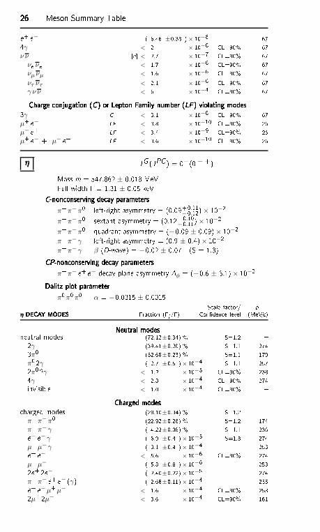
26262626 Meson Summary Tablee+ e− ( 6.46 ±0.33 )× 10−8 674γ < 2 × 10⁻⁸ CL=90% 67ν ν [e < 2.7 × 10⁻⁷ CL=90% 67
νe νe < 1.7 × 10⁻⁶ CL=90% 67νµ νµ < 1.6 × 10⁻⁶ CL=90% 67ντ ντ < 2.1 × 10⁻⁶ CL=90% 67γ ν ν < 6 × 10⁻⁴ CL=90% 67Charge onjugation (C ) or Lepton Family number (LF ) violating modesCharge onjugation (C ) or Lepton Family number (LF ) violating modesCharge onjugation (C ) or Lepton Family number (LF ) violating modesCharge onjugation (C ) or Lepton Family number (LF ) violating modes3γ C < 3.1 × 10⁻⁸ CL=90% 67
µ+ e− LF < 3.8 × 10⁻¹⁰ CL=90% 26µ− e+ LF < 3.4 × 10⁻⁹ CL=90% 26µ+ e− + µ− e+ LF < 3.6 × 10⁻¹⁰ CL=90% 26ηηηη IG (JPC ) = 0+(0−+)Mass m = 547.862 ± 0.018 MeVFull width = 1.31 ± 0.05 keVC-non onserving de ay parametersC-non onserving de ay parametersC-non onserving de ay parametersC-non onserving de ay parameters
π+π−π0 left-right asymmetry = (0.09+0.11−0.12)× 10−2
π+π−π0 sextant asymmetry = (0.12+0.10−0.11)× 10−2
π+π−π0 quadrant asymmetry = (−0.09 ± 0.09)× 10−2π+π− γ left-right asymmetry = (0.9 ± 0.4)× 10−2π+π− γ β (D-wave) = −0.02 ± 0.07 (S = 1.3)CP-non onserving de ay parametersCP-non onserving de ay parametersCP-non onserving de ay parametersCP-non onserving de ay parametersπ+π− e+ e− de ay-plane asymmetry Aφ = (−0.6 ± 3.1)× 10−2Dalitz plot parameterDalitz plot parameterDalitz plot parameterDalitz plot parameterπ0π0π0 α = −0.0315 ± 0.0015 S ale fa tor/ p
η DECAY MODESη DECAY MODESη DECAY MODESη DECAY MODES Fra tion (i /) Conden e level (MeV/ )Neutral modesNeutral modesNeutral modesNeutral modesneutral modes (72.12±0.34) % S=1.2 2γ (39.41±0.20) % S=1.1 2743π0 (32.68±0.23) % S=1.1 179π0 2γ ( 2.7 ±0.5 )× 10−4 S=1.1 2572π0 2γ < 1.2 × 10⁻³ CL=90% 2384γ < 2.8 × 10⁻⁴ CL=90% 274invisible < 1.0 × 10⁻⁴ CL=90% Charged modesCharged modesCharged modesCharged modes harged modes (28.10±0.34) % S=1.2 π+π−π0 (22.92±0.28) % S=1.2 174π+π−γ ( 4.22±0.08) % S=1.1 236e+ e−γ ( 6.9 ±0.4 )× 10−3 S=1.3 274µ+µ− γ ( 3.1 ±0.4 )× 10−4 253e+ e− < 5.6 × 10⁻⁶ CL=90% 274µ+µ− ( 5.8 ±0.8 )× 10−6 2532e+2e− ( 2.40±0.22)× 10−5 274π+π− e+ e− (γ) ( 2.68±0.11)× 10−4 235e+ e−µ+µ− < 1.6 × 10⁻⁴ CL=90% 2532µ+2µ− < 3.6 × 10⁻⁴ CL=90% 161

Meson Summary Table 27272727µ+µ−π+π− < 3.6 × 10⁻⁴ CL=90% 113π+ e−νe+ . . < 1.7 × 10⁻⁴ CL=90% 256π+π−2γ < 2.1 × 10⁻³ 236π+π−π0 γ < 5 × 10⁻⁴ CL=90% 174π0µ+µ−γ < 3 × 10⁻⁶ CL=90% 210Charge onjugation (C ), Parity (P),Charge onjugation (C ), Parity (P),Charge onjugation (C ), Parity (P),Charge onjugation (C ), Parity (P),Charge onjugation × Parity (CP), orCharge onjugation × Parity (CP), orCharge onjugation × Parity (CP), orCharge onjugation × Parity (CP), orLepton Family number (LF ) violating modesLepton Family number (LF ) violating modesLepton Family number (LF ) violating modesLepton Family number (LF ) violating modes
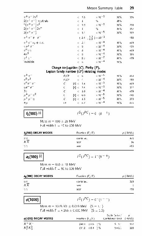
π0 γ C < 9 × 10⁻⁵ CL=90% 257π+π− P,CP < 1.3 × 10⁻⁵ CL=90% 2362π0 P,CP < 3.5 × 10⁻⁴ CL=90% 2382π0 γ C < 5 × 10⁻⁴ CL=90% 2383π0 γ C < 6 × 10⁻⁵ CL=90% 1793γ C < 1.6 × 10⁻⁵ CL=90% 2744π0 P,CP < 6.9 × 10⁻⁷ CL=90% 40π0 e+ e− C [f < 4 × 10⁻⁵ CL=90% 257π0µ+µ− C [f < 5 × 10⁻⁶ CL=90% 210µ+ e− + µ− e+ LF < 6 × 10⁻⁶ CL=90% 264f0(500) or σf0(500) or σf0(500) or σf0(500) or σ
[g was f0(600)was f0(600)was f0(600)was f0(600) IG (JPC ) = 0+(0 + +)Mass m = (400550) MeVFull width = (400700) MeVf0(500) DECAY MODESf0(500) DECAY MODESf0(500) DECAY MODESf0(500) DECAY MODES Fra tion (i /) p (MeV/ )ππ dominant γ γ seen ρ(770)ρ(770)ρ(770)ρ(770) [h IG (JPC ) = 1+(1−−)Mass m = 775.26 ± 0.25 MeVFull width = 149.1 ± 0.8 MeVee = 7.04 ± 0.06 keV S ale fa tor/ p
ρ(770) DECAY MODESρ(770) DECAY MODESρ(770) DECAY MODESρ(770) DECAY MODES Fra tion (i /) Conden e level (MeV/ )ππ ∼ 100 % 363
ρ(770)± de aysρ(770)± de aysρ(770)± de aysρ(770)± de aysπ± γ ( 4.5 ±0.5 )× 10−4 S=2.2 375π± η < 6 × 10⁻³ CL=84% 152π±π+π−π0 < 2.0 × 10⁻³ CL=84% 254
ρ(770)0 de aysρ(770)0 de aysρ(770)0 de aysρ(770)0 de aysπ+π−γ ( 9.9 ±1.6 )× 10−3 362π0 γ ( 6.0 ±0.8 )× 10−4 376ηγ ( 3.00±0.20 )× 10−4 194π0π0 γ ( 4.5 ±0.8 )× 10−5 363µ+µ− [i ( 4.55±0.28 )× 10−5 373
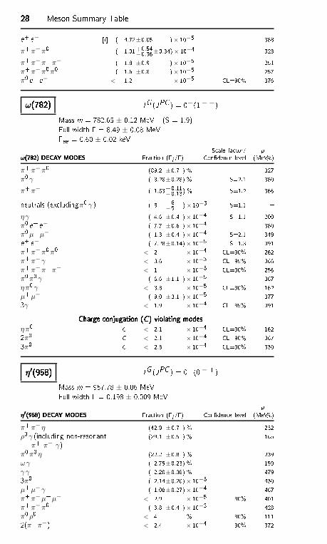
28282828 Meson Summary Tablee+ e− [i ( 4.72±0.05 )× 10−5 388π+π−π0 ( 1.01+0.54
−0.36±0.34)× 10−4 323π+π−π+π− ( 1.8 ±0.9 )× 10−5 251π+π−π0π0 ( 1.6 ±0.8 )× 10−5 257π0 e+ e− < 1.2 × 10⁻⁵ CL=90% 376ω(782)ω(782)ω(782)ω(782) IG (JPC ) = 0−(1−−)Mass m = 782.65 ± 0.12 MeV (S = 1.9)Full width = 8.49 ± 0.08 MeVee = 0.60 ± 0.02 keV S ale fa tor/ p
ω(782) DECAY MODESω(782) DECAY MODESω(782) DECAY MODESω(782) DECAY MODES Fra tion (i /) Conden e level (MeV/ )π+π−π0 (89.2 ±0.7 ) % 327π0 γ ( 8.28±0.28) % S=2.1 380π+π− ( 1.53+0.11
−0.13) % S=1.2 366neutrals (ex ludingπ0 γ ) ( 8 +8−5 )× 10−3 S=1.1
ηγ ( 4.6 ±0.4 )× 10−4 S=1.1 200π0 e+ e− ( 7.7 ±0.6 )× 10−4 380π0µ+µ− ( 1.3 ±0.4 )× 10−4 S=2.1 349e+ e− ( 7.28±0.14)× 10−5 S=1.3 391π+π−π0π0 < 2 × 10⁻⁴ CL=90% 262π+π−γ < 3.6 × 10⁻³ CL=95% 366π+π−π+π− < 1 × 10⁻³ CL=90% 256π0π0 γ ( 6.6 ±1.1 )× 10−5 367ηπ0 γ < 3.3 × 10⁻⁵ CL=90% 162µ+µ− ( 9.0 ±3.1 )× 10−5 3773γ < 1.9 × 10⁻⁴ CL=95% 391Charge onjugation (C ) violating modesCharge onjugation (C ) violating modesCharge onjugation (C ) violating modesCharge onjugation (C ) violating modesηπ0 C < 2.1 × 10⁻⁴ CL=90% 1622π0 C < 2.1 × 10⁻⁴ CL=90% 3673π0 C < 2.3 × 10⁻⁴ CL=90% 330η′(958)η′(958)η′(958)η′(958) IG (JPC ) = 0+(0−+)Mass m = 957.78 ± 0.06 MeVFull width = 0.198 ± 0.009 MeV p
η′(958) DECAY MODESη′(958) DECAY MODESη′(958) DECAY MODESη′(958) DECAY MODES Fra tion (i /) Conden e level (MeV/ )π+π−η (42.9 ±0.7 ) % 232ρ0 γ (in luding non-resonant
π+ π− γ) (29.1 ±0.5 ) % 165π0π0 η (22.2 ±0.8 ) % 239ωγ ( 2.75±0.23) % 159γ γ ( 2.20±0.08) % 4793π0 ( 2.14±0.20)× 10−3 430µ+µ− γ ( 1.08±0.27)× 10−4 467π+π−µ+µ− < 2.9 × 10⁻⁵ 90% 401π+π−π0 ( 3.8 ±0.4 )× 10−3 428π0 ρ0 < 4 % 90% 1112(π+π−) < 2.4 × 10⁻⁴ 90% 372
Meson Summary Table 29292929π+π−2π0 < 2.5 × 10⁻³ 90% 3762(π+π−) neutrals < 1 % 95% 2(π+π−)π0 < 1.9 × 10⁻³ 90% 2982(π+π−)2π0 < 1 % 95% 1973(π+π−) < 3.1 × 10⁻⁵ 90% 189π+π− e+ e− ( 2.4 +1.3
−1.0 )× 10−3 458π+ e−νe+ . . < 2.1 × 10⁻⁴ 90% 469γ e+ e− < 9 × 10⁻⁴ 90% 479π0 γ γ < 8 × 10⁻⁴ 90% 4694π0 < 5 × 10⁻⁴ 90% 380e+ e− < 2.1 × 10⁻⁷ 90% 479invisible < 5 × 10⁻⁴ 90% Charge onjugation (C ), Parity (P),Charge onjugation (C ), Parity (P),Charge onjugation (C ), Parity (P),Charge onjugation (C ), Parity (P),Lepton family number (LF ) violating modesLepton family number (LF ) violating modesLepton family number (LF ) violating modesLepton family number (LF ) violating modesπ+π− P,CP < 6 × 10⁻⁵ 90% 458π0π0 P,CP < 4 × 10⁻⁴ 90% 459π0 e+ e− C [f < 1.4 × 10⁻³ 90% 469ηe+ e− C [f < 2.4 × 10⁻³ 90% 3223γ C < 1.0 × 10⁻⁴ 90% 479µ+µ−π0 C [f < 6.0 × 10⁻⁵ 90% 445µ+µ− η C [f < 1.5 × 10⁻⁵ 90% 273eµ LF < 4.7 × 10⁻⁴ 90% 473f0(980)f0(980)f0(980)f0(980) [j IG (JPC ) = 0+(0 + +)Mass m = 990 ± 20 MeVFull width = 40 to 100 MeVf0(980) DECAY MODESf0(980) DECAY MODESf0(980) DECAY MODESf0(980) DECAY MODES Fra tion (i /) p (MeV/ )ππ dominant 476K K seen 36γ γ seen 495a0(980)a0(980)a0(980)a0(980) [j IG (JPC ) = 1−(0 + +)Mass m = 980 ± 20 MeVFull width = 50 to 100 MeVa0(980) DECAY MODESa0(980) DECAY MODESa0(980) DECAY MODESa0(980) DECAY MODES Fra tion (i /) p (MeV/ )ηπ dominant 319K K seen †γ γ seen 490φ(1020)φ(1020)φ(1020)φ(1020) IG (JPC ) = 0−(1−−)Mass m = 1019.461 ± 0.019 MeV (S = 1.1)Full width = 4.266 ± 0.031 MeV (S = 1.2) S ale fa tor/ p
φ(1020) DECAY MODESφ(1020) DECAY MODESφ(1020) DECAY MODESφ(1020) DECAY MODES Fra tion (i /) Conden e level (MeV/ )K+K− (48.9 ±0.5 ) % S=1.1 127K0LK0S (34.2 ±0.4 ) % S=1.1 110
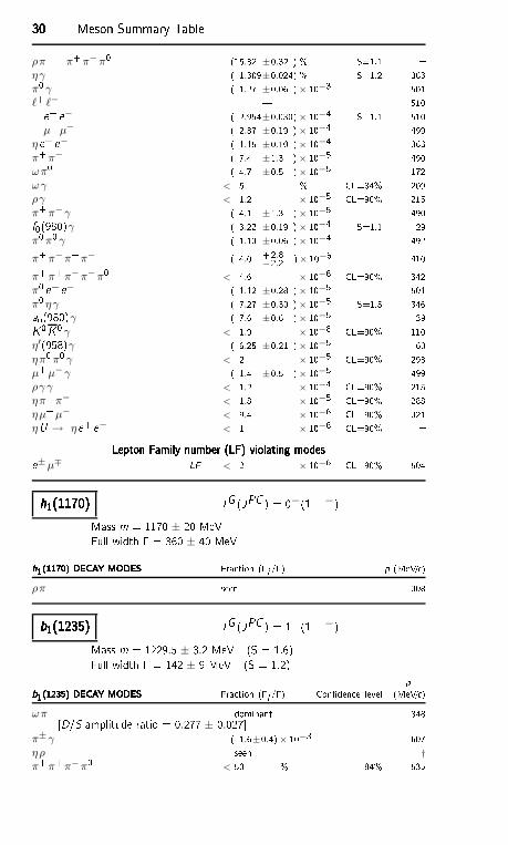
30303030 Meson Summary Tableρπ + π+π−π0 (15.32 ±0.32 ) % S=1.1 ηγ ( 1.309±0.024) % S=1.2 363π0 γ ( 1.27 ±0.06 )× 10−3 501ℓ+ ℓ− | 510e+ e− ( 2.954±0.030)× 10−4 S=1.1 510
µ+µ− ( 2.87 ±0.19 )× 10−4 499ηe+ e− ( 1.15 ±0.10 )× 10−4 363π+π− ( 7.4 ±1.3 )× 10−5 490ωπ0 ( 4.7 ±0.5 )× 10−5 172ωγ < 5 % CL=84% 209ργ < 1.2 × 10⁻⁵ CL=90% 215π+π−γ ( 4.1 ±1.3 )× 10−5 490f0(980)γ ( 3.22 ±0.19 )× 10−4 S=1.1 29π0π0 γ ( 1.13 ±0.06 )× 10−4 492π+π−π+π− ( 4.0 +2.8
−2.2 )× 10−6 410π+π+π−π−π0 < 4.6 × 10⁻⁶ CL=90% 342π0 e+ e− ( 1.12 ±0.28 )× 10−5 501π0 ηγ ( 7.27 ±0.30 )× 10−5 S=1.5 346a0(980)γ ( 7.6 ±0.6 )× 10−5 39K0K0 γ < 1.9 × 10⁻⁸ CL=90% 110η′(958)γ ( 6.25 ±0.21 )× 10−5 60ηπ0π0 γ < 2 × 10⁻⁵ CL=90% 293µ+µ− γ ( 1.4 ±0.5 )× 10−5 499ργ γ < 1.2 × 10⁻⁴ CL=90% 215ηπ+π− < 1.8 × 10⁻⁵ CL=90% 288ηµ+µ− < 9.4 × 10⁻⁶ CL=90% 321ηU → ηe+ e− < 1 × 10⁻⁶ CL=90% Lepton Family number (LF) violating modesLepton Family number (LF) violating modesLepton Family number (LF) violating modesLepton Family number (LF) violating modese±µ∓ LF < 2 × 10⁻⁶ CL=90% 504h1(1170)h1(1170)h1(1170)h1(1170) IG (JPC ) = 0−(1 +−)Mass m = 1170 ± 20 MeVFull width = 360 ± 40 MeVh1(1170) DECAY MODESh1(1170) DECAY MODESh1(1170) DECAY MODESh1(1170) DECAY MODES Fra tion (i /) p (MeV/ )ρπ seen 308b1(1235)b1(1235)b1(1235)b1(1235) IG (JPC ) = 1+(1 +−)Mass m = 1229.5 ± 3.2 MeV (S = 1.6)Full width = 142 ± 9 MeV (S = 1.2) pb1(1235) DECAY MODESb1(1235) DECAY MODESb1(1235) DECAY MODESb1(1235) DECAY MODES Fra tion (i /) Conden e level (MeV/ )ωπ dominant 348[D/S amplitude ratio = 0.277 ± 0.027π± γ ( 1.6±0.4)× 10−3 607ηρ seen †π+π+π−π0 < 50 % 84% 535
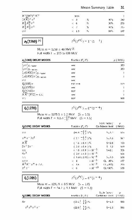
Meson Summary Table 31313131K∗(892)±K∓ seen †(KK )±π0 < 8 % 90% 248K0S K0Lπ± < 6 % 90% 235K0S K0S π± < 2 % 90% 235φπ < 1.5 % 84% 147a1(1260)a1(1260)a1(1260)a1(1260) [k IG (JPC ) = 1−(1 + +)Mass m = 1230 ± 40 MeV [lFull width = 250 to 600 MeVa1(1260) DECAY MODESa1(1260) DECAY MODESa1(1260) DECAY MODESa1(1260) DECAY MODES Fra tion (i /) p (MeV/ )(ρπ)S−wave seen 353(ρπ)D−wave seen 353(ρ(1450)π )S−wave seen †(ρ(1450)π )D−wave seen †σπ seen f0(980)π not seen 179f0(1370)π seen †f2(1270)π seen †K K∗(892)+ . . seen †πγ seen 608f2(1270)f2(1270)f2(1270)f2(1270) IG (JPC ) = 0+(2 + +)Mass m = 1275.1 ± 1.2 MeV (S = 1.1)Full width = 185.1+2.9
−2.4 MeV (S = 1.5) S ale fa tor/ pf2(1270) DECAY MODESf2(1270) DECAY MODESf2(1270) DECAY MODESf2(1270) DECAY MODES Fra tion (i /) Conden e level (MeV/ )ππ (84.8 +2.4
−1.2 ) % S=1.2 623π+π−2π0 ( 7.1 +1.4
−2.7 ) % S=1.3 562K K ( 4.6 ±0.4 ) % S=2.8 4032π+2π− ( 2.8 ±0.4 ) % S=1.2 559ηη ( 4.0 ±0.8 )× 10−3 S=2.1 3264π0 ( 3.0 ±1.0 )× 10−3 564γ γ ( 1.64±0.19)× 10−5 S=1.9 638ηππ < 8 × 10⁻³ CL=95% 477K0K−π++ . . < 3.4 × 10⁻³ CL=95% 293e+ e− < 6 × 10⁻¹⁰ CL=90% 638f1(1285)f1(1285)f1(1285)f1(1285) IG (JPC ) = 0+(1 + +)Mass m = 1281.9 ± 0.5 MeV (S = 1.8)Full width = 24.2 ± 1.1 MeV (S = 1.3) S ale fa tor/ pf1(1285) DECAY MODESf1(1285) DECAY MODESf1(1285) DECAY MODESf1(1285) DECAY MODES Fra tion (i /) Conden e level (MeV/ )4π (33.1+ 2.1
− 1.8) % S=1.3 568π0π0π+π− (22.0+ 1.4
− 1.2) % S=1.3 566
32323232 Meson Summary Table2π+2π− (11.0+ 0.7− 0.6) % S=1.3 563
ρ0π+π− (11.0+ 0.7− 0.6) % S=1.3 336
ρ0 ρ0 seen †4π0 < 7 × 10⁻⁴ CL=90% 568ηπ+π− (35 ±15 ) % 479ηππ (52.4+ 1.9
− 2.2) % S=1.2 482a0(980)π [ignoring a0(980) →K K (36 ± 7 ) % 238ηππ [ex luding a0(980)π (16 ± 7 ) % 482K K π ( 9.0± 0.4) % S=1.1 308K K∗(892) not seen †
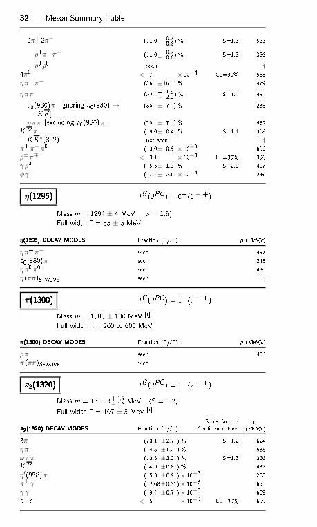
π+π−π0 ( 3.0± 0.9)× 10−3 603ρ±π∓ < 3.1 × 10⁻³ CL=95% 390γ ρ0 ( 5.5± 1.3) % S=2.8 407φγ ( 7.4± 2.6)× 10−4 236η(1295)η(1295)η(1295)η(1295) IG (JPC ) = 0+(0−+)Mass m = 1294 ± 4 MeV (S = 1.6)Full width = 55 ± 5 MeV
η(1295) DECAY MODESη(1295) DECAY MODESη(1295) DECAY MODESη(1295) DECAY MODES Fra tion (i /) p (MeV/ )ηπ+π− seen 487a0(980)π seen 248ηπ0π0 seen 490η (ππ)S-wave seen π(1300)π(1300)π(1300)π(1300) IG (JPC ) = 1−(0−+)Mass m = 1300 ± 100 MeV [lFull width = 200 to 600 MeV
π(1300) DECAY MODESπ(1300) DECAY MODESπ(1300) DECAY MODESπ(1300) DECAY MODES Fra tion (i /) p (MeV/ )ρπ seen 404π (ππ)S-wave seen a2(1320)a2(1320)a2(1320)a2(1320) IG (JPC ) = 1−(2 + +)Mass m = 1318.3+0.5
−0.6 MeV (S = 1.2)Full width = 107 ± 5 MeV [l S ale fa tor/ pa2(1320) DECAY MODESa2(1320) DECAY MODESa2(1320) DECAY MODESa2(1320) DECAY MODES Fra tion (i /) Conden e level (MeV/ )3π (70.1 ±2.7 ) % S=1.2 624ηπ (14.5 ±1.2 ) % 535ωππ (10.6 ±3.2 ) % S=1.3 366K K ( 4.9 ±0.8 ) % 437η′(958)π ( 5.3 ±0.9 )× 10−3 288π± γ ( 2.68±0.31)× 10−3 652γ γ ( 9.4 ±0.7 )× 10−6 659e+ e− < 5 × 10⁻⁹ CL=90% 659
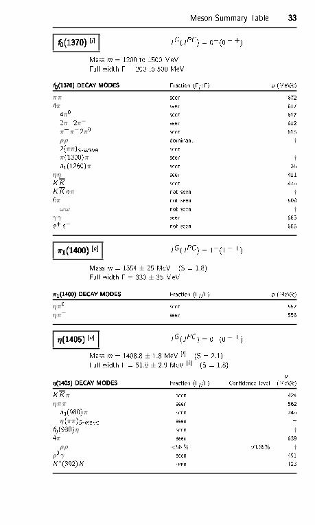
Meson Summary Table 33333333f0(1370)f0(1370)f0(1370)f0(1370) [j IG (JPC ) = 0+(0 + +)Mass m = 1200 to 1500 MeVFull width = 200 to 500 MeVf0(1370) DECAY MODESf0(1370) DECAY MODESf0(1370) DECAY MODESf0(1370) DECAY MODES Fra tion (i /) p (MeV/ )ππ seen 6724π seen 6174π0 seen 6172π+2π− seen 612
π+π−2π0 seen 615ρρ dominant †2(ππ)S-wave seen π(1300)π seen †a1(1260)π seen 35
ηη seen 411K K seen 475K K nπ not seen †6π not seen 508ωω not seen †
γ γ seen 685e+ e− not seen 685π1(1400)π1(1400)π1(1400)π1(1400) [n IG (JPC ) = 1−(1−+)Mass m = 1354 ± 25 MeV (S = 1.8)Full width = 330 ± 35 MeV
π1(1400) DECAY MODESπ1(1400) DECAY MODESπ1(1400) DECAY MODESπ1(1400) DECAY MODES Fra tion (i /) p (MeV/ )ηπ0 seen 557ηπ− seen 556η(1405)η(1405)η(1405)η(1405) [o IG (JPC ) = 0+(0−+)Mass m = 1408.8 ± 1.8 MeV [l (S = 2.1)Full width = 51.0 ± 2.9 MeV [l (S = 1.8) p
η(1405) DECAY MODESη(1405) DECAY MODESη(1405) DECAY MODESη(1405) DECAY MODES Fra tion (i /) Conden e level (MeV/ )K K π seen 424ηππ seen 562a0(980)π seen 345
η (ππ)S-wave seen f0(980)η seen †4π seen 639ρρ <58 % 99.85% †
ρ0 γ seen 491K∗(892)K seen 123
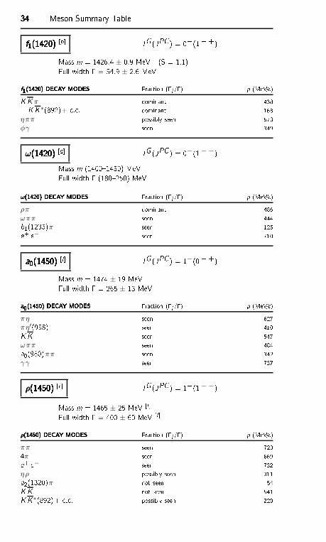
34343434 Meson Summary Tablef1(1420)f1(1420)f1(1420)f1(1420) [p IG (JPC ) = 0+(1 + +)Mass m = 1426.4 ± 0.9 MeV (S = 1.1)Full width = 54.9 ± 2.6 MeVf1(1420) DECAY MODESf1(1420) DECAY MODESf1(1420) DECAY MODESf1(1420) DECAY MODES Fra tion (i /) p (MeV/ )K K π dominant 438K K∗(892)+ . . dominant 163ηππ possibly seen 573φγ seen 349ω(1420)ω(1420)ω(1420)ω(1420) [q IG (JPC ) = 0−(1−−)Mass m (14001450) MeVFull width (180250) MeV
ω(1420) DECAY MODESω(1420) DECAY MODESω(1420) DECAY MODESω(1420) DECAY MODES Fra tion (i /) p (MeV/ )ρπ dominant 486ωππ seen 444b1(1235)π seen 125e+ e− seen 710a0(1450)a0(1450)a0(1450)a0(1450) [j IG (JPC ) = 1−(0 + +)Mass m = 1474 ± 19 MeVFull width = 265 ± 13 MeVa0(1450) DECAY MODESa0(1450) DECAY MODESa0(1450) DECAY MODESa0(1450) DECAY MODES Fra tion (i /) p (MeV/ )πη seen 627πη′(958) seen 410K K seen 547ωππ seen 484a0(980)ππ seen 342γ γ seen 737ρ(1450)ρ(1450)ρ(1450)ρ(1450) [r IG (JPC ) = 1+(1−−)Mass m = 1465 ± 25 MeV [lFull width = 400 ± 60 MeV [l
ρ(1450) DECAY MODESρ(1450) DECAY MODESρ(1450) DECAY MODESρ(1450) DECAY MODES Fra tion (i /) p (MeV/ )ππ seen 7204π seen 669e+ e− seen 732ηρ possibly seen 311a2(1320)π not seen 54K K not seen 541K K∗(892)+ . . possibly seen 229

Meson Summary Table 35353535ηγ possibly seen 630f0(500)γ not seen f0(980)γ not seen 398f0(1370)γ not seen 92f2(1270)γ not seen 178η(1475)η(1475)η(1475)η(1475) [o IG (JPC ) = 0+(0−+)Mass m = 1476 ± 4 MeV (S = 1.3)Full width = 85 ± 9 MeV (S = 1.5)
η(1475) DECAY MODESη(1475) DECAY MODESη(1475) DECAY MODESη(1475) DECAY MODES Fra tion (i /) p (MeV/ )K K π dominant 477K K∗(892)+ . . seen 245a0(980)π seen 396γ γ seen 738f0(1500)f0(1500)f0(1500)f0(1500) [n IG (JPC ) = 0+(0 + +)Mass m = 1505 ± 6 MeV (S = 1.3)Full width = 109 ± 7 MeV pf0(1500) DECAY MODESf0(1500) DECAY MODESf0(1500) DECAY MODESf0(1500) DECAY MODES Fra tion (i /) S ale fa tor (MeV/ )ππ (34.9±2.3) % 1.2 741
π+π− seen 7402π0 seen 7414π (49.5±3.3) % 1.2 6914π0 seen 6912π+2π− seen 6872(ππ)S-wave seen ρρ seen †π(1300)π seen 144a1(1260)π seen 218
ηη ( 5.1±0.9) % 1.4 516ηη′(958) ( 1.9±0.8) % 1.7 †K K ( 8.6±1.0) % 1.1 568γ γ not seen 753f ′2(1525)f ′2(1525)f ′2(1525)f ′2(1525) IG (JPC ) = 0+(2 + +)Mass m = 1525 ± 5 MeV [lFull width = 73+6
−5 MeV [lf ′2(1525) DECAY MODESf ′2(1525) DECAY MODESf ′2(1525) DECAY MODESf ′2(1525) DECAY MODES Fra tion (i /) p (MeV/ )K K (88.7 ±2.2 ) % 581ηη (10.4 ±2.2 ) % 530ππ ( 8.2 ±1.5 )× 10−3 750γ γ ( 1.10±0.14)× 10−6 763
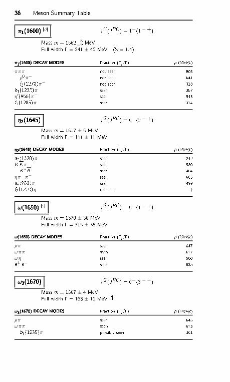
36363636 Meson Summary Tableπ1(1600)π1(1600)π1(1600)π1(1600) [n IG (JPC ) = 1−(1−+)Mass m = 1662+8
−9 MeVFull width = 241 ± 40 MeV (S = 1.4)π1(1600) DECAY MODESπ1(1600) DECAY MODESπ1(1600) DECAY MODESπ1(1600) DECAY MODES Fra tion (i /) p (MeV/ )πππ not seen 803
ρ0π− not seen 641f2(1270)π− not seen 318b1(1235)π seen 357η′(958)π− seen 543f1(1285)π seen 314η2(1645)η2(1645)η2(1645)η2(1645) IG (JPC ) = 0+(2−+)Mass m = 1617 ± 5 MeVFull width = 181 ± 11 MeV
η2(1645) DECAY MODESη2(1645) DECAY MODESη2(1645) DECAY MODESη2(1645) DECAY MODES Fra tion (i /) p (MeV/ )a2(1320)π seen 242K K π seen 580K∗K seen 404ηπ+π− seen 685a0(980)π seen 499f2(1270)η not seen †
ω(1650)ω(1650)ω(1650)ω(1650) [s IG (JPC ) = 0−(1−−)Mass m = 1670 ± 30 MeVFull width = 315 ± 35 MeVω(1650) DECAY MODESω(1650) DECAY MODESω(1650) DECAY MODESω(1650) DECAY MODES Fra tion (i /) p (MeV/ )ρπ seen 647ωππ seen 617ωη seen 500e+ e− seen 835ω3(1670)ω3(1670)ω3(1670)ω3(1670) IG (JPC ) = 0−(3−−)Mass m = 1667 ± 4 MeVFull width = 168 ± 10 MeV [l
ω3(1670) DECAY MODESω3(1670) DECAY MODESω3(1670) DECAY MODESω3(1670) DECAY MODES Fra tion (i /) p (MeV/ )ρπ seen 645ωππ seen 615b1(1235)π possibly seen 361
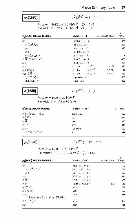
Meson Summary Table 37373737π2(1670)π2(1670)π2(1670)π2(1670) IG (JPC ) = 1−(2−+)Mass m = 1672.2 ± 3.0 MeV [l (S = 1.4)Full width = 260 ± 9 MeV [l (S = 1.2) p
π2(1670) DECAY MODESπ2(1670) DECAY MODESπ2(1670) DECAY MODESπ2(1670) DECAY MODES Fra tion (i /) Conden e level (MeV/ )3π (95.8±1.4) % 809f2(1270)π (56.3±3.2) % 329ρπ (31 ±4 ) % 648σπ (10.9±3.4) % (ππ)S-wave ( 8.7±3.4) % K K∗(892)+ . . ( 4.2±1.4) % 455
ωρ ( 2.7±1.1) % 304γ γ < 2.8 × 10⁻⁷ 90% 836ρ(1450)π < 3.6 × 10⁻³ 97.7% 147b1(1235)π < 1.9 × 10⁻³ 97.7% 365f1(1285)π possibly seen 323a2(1320)π not seen 292φ(1680)φ(1680)φ(1680)φ(1680) IG (JPC ) = 0−(1−−)Mass m = 1680 ± 20 MeV [lFull width = 150 ± 50 MeV [l
φ(1680) DECAY MODESφ(1680) DECAY MODESφ(1680) DECAY MODESφ(1680) DECAY MODES Fra tion (i /) p (MeV/ )K K∗(892)+ . . dominant 462K0S K π seen 621K K seen 680e+ e− seen 840ωππ not seen 623K+K−π+π− seen 544ρ3(1690)ρ3(1690)ρ3(1690)ρ3(1690) IG (JPC ) = 1+(3−−)Mass m = 1688.8 ± 2.1 MeV [lFull width = 161 ± 10 MeV [l (S = 1.5) p
ρ3(1690) DECAY MODESρ3(1690) DECAY MODESρ3(1690) DECAY MODESρ3(1690) DECAY MODES Fra tion (i /) S ale fa tor (MeV/ )4π (71.1 ± 1.9 ) % 790π±π+π−π0 (67 ±22 ) % 787ωπ (16 ± 6 ) % 655
ππ (23.6 ± 1.3 ) % 834K K π ( 3.8 ± 1.2 ) % 629K K ( 1.58± 0.26) % 1.2 685ηπ+π− seen 727ρ(770)η seen 520ππρ seen 633Ex luding 2ρ and a2(1320)π.a2(1320)π seen 307ρρ seen 335
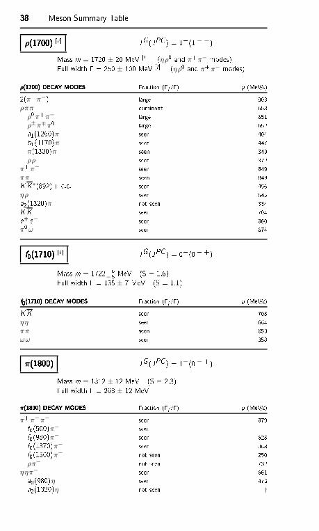
38383838 Meson Summary Tableρ(1700)ρ(1700)ρ(1700)ρ(1700) [r IG (JPC ) = 1+(1−−)Mass m = 1720 ± 20 MeV [l (ηρ0 and π+π− modes)Full width = 250 ± 100 MeV [l (ηρ0 and π+π− modes)
ρ(1700) DECAY MODESρ(1700) DECAY MODESρ(1700) DECAY MODESρ(1700) DECAY MODES Fra tion (i /) p (MeV/ )2(π+π−) large 803ρππ dominant 653
ρ0π+π− large 651ρ±π∓π0 large 652a1(1260)π seen 404h1(1170)π seen 447π(1300)π seen 349ρρ seen 372
π+π− seen 849ππ seen 849K K∗(892)+ . . seen 496ηρ seen 545a2(1320)π not seen 334K K seen 704e+ e− seen 860π0ω seen 674f0(1710)f0(1710)f0(1710)f0(1710) [t IG (JPC ) = 0+(0 + +)Mass m = 1722+6
−5 MeV (S = 1.6)Full width = 135 ± 7 MeV (S = 1.1)f0(1710) DECAY MODESf0(1710) DECAY MODESf0(1710) DECAY MODESf0(1710) DECAY MODES Fra tion (i /) p (MeV/ )K K seen 705ηη seen 664ππ seen 850ωω seen 358π(1800)π(1800)π(1800)π(1800) IG (JPC ) = 1−(0−+)Mass m = 1812 ± 12 MeV (S = 2.3)Full width = 208 ± 12 MeV
π(1800) DECAY MODESπ(1800) DECAY MODESπ(1800) DECAY MODESπ(1800) DECAY MODES Fra tion (i /) p (MeV/ )π+π−π− seen 879f0(500)π− seen f0(980)π− seen 625f0(1370)π− seen 368f0(1500)π− not seen 250
ρπ− not seen 732ηηπ− seen 661a0(980)η seen 473a2(1320)η not seen †
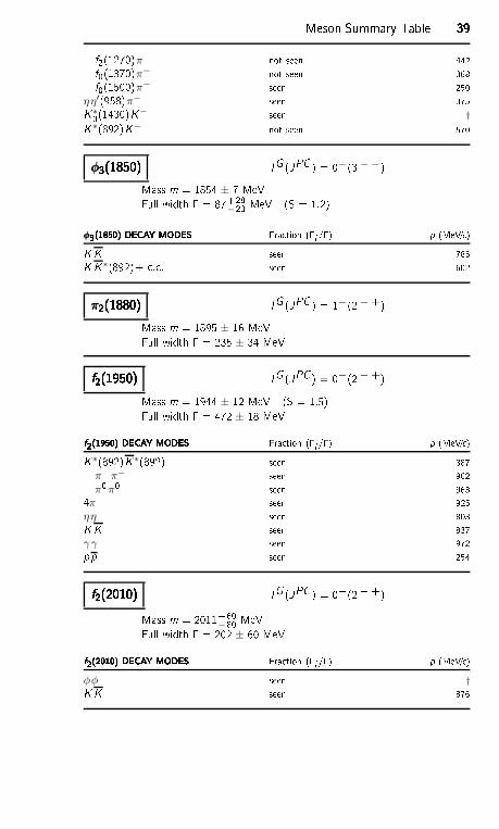
Meson Summary Table 39393939f2(1270)π not seen 442f0(1370)π− not seen 368f0(1500)π− seen 250ηη′(958)π− seen 375K∗0(1430)K− seen †K∗(892)K− not seen 570φ3(1850)φ3(1850)φ3(1850)φ3(1850) IG (JPC ) = 0−(3−−)Mass m = 1854 ± 7 MeVFull width = 87+28
−23 MeV (S = 1.2)φ3(1850) DECAY MODESφ3(1850) DECAY MODESφ3(1850) DECAY MODESφ3(1850) DECAY MODES Fra tion (i /) p (MeV/ )K K seen 785K K∗(892)+ . . seen 602π2(1880)π2(1880)π2(1880)π2(1880) IG (JPC ) = 1−(2−+)Mass m = 1895 ± 16 MeVFull width = 235 ± 34 MeVf2(1950)f2(1950)f2(1950)f2(1950) IG (JPC ) = 0+(2 + +)Mass m = 1944 ± 12 MeV (S = 1.5)Full width = 472 ± 18 MeVf2(1950) DECAY MODESf2(1950) DECAY MODESf2(1950) DECAY MODESf2(1950) DECAY MODES Fra tion (i /) p (MeV/ )K∗(892)K∗(892) seen 387π+π− seen 962π0π0 seen 9634π seen 925
ηη seen 803K K seen 837γ γ seen 972pp seen 254f2(2010)f2(2010)f2(2010)f2(2010) IG (JPC ) = 0+(2 + +)Mass m = 2011+60
−80 MeVFull width = 202 ± 60 MeVf2(2010) DECAY MODESf2(2010) DECAY MODESf2(2010) DECAY MODESf2(2010) DECAY MODES Fra tion (i /) p (MeV/ )φφ seen †K K seen 876
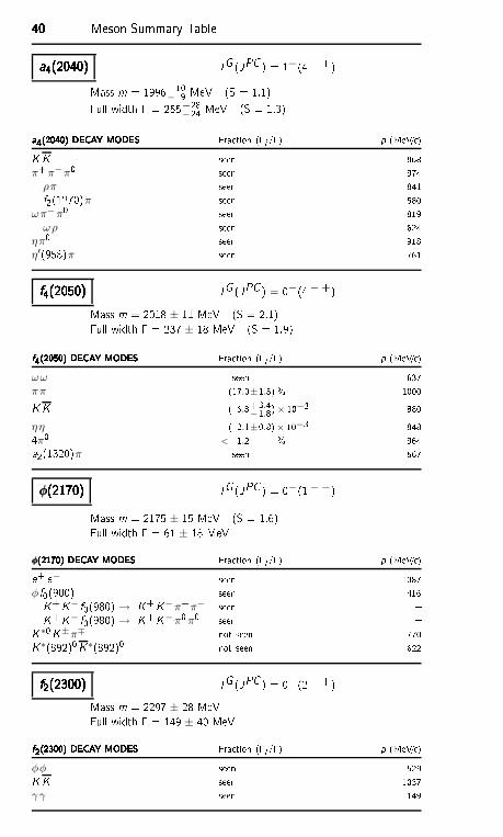
40404040 Meson Summary Tablea4(2040)a4(2040)a4(2040)a4(2040) IG (JPC ) = 1−(4 + +)Mass m = 1996+10− 9 MeV (S = 1.1)Full width = 255+28
−24 MeV (S = 1.3)a4(2040) DECAY MODESa4(2040) DECAY MODESa4(2040) DECAY MODESa4(2040) DECAY MODES Fra tion (i /) p (MeV/ )K K seen 868π+π−π0 seen 974
ρπ seen 841f2(1270)π seen 580ωπ−π0 seen 819
ωρ seen 624ηπ0 seen 918η′(958)π seen 761f4(2050)f4(2050)f4(2050)f4(2050) IG (JPC ) = 0+(4 + +)Mass m = 2018 ± 11 MeV (S = 2.1)Full width = 237 ± 18 MeV (S = 1.9)f4(2050) DECAY MODESf4(2050) DECAY MODESf4(2050) DECAY MODESf4(2050) DECAY MODES Fra tion (i /) p (MeV/ )ωω seen 637ππ (17.0±1.5) % 1000K K ( 6.8+3.4
−1.8)× 10−3 880ηη ( 2.1±0.8)× 10−3 8484π0 < 1.2 % 964a2(1320)π seen 567φ(2170)φ(2170)φ(2170)φ(2170) IG (JPC ) = 0−(1−−)Mass m = 2175 ± 15 MeV (S = 1.6)Full width = 61 ± 18 MeV
φ(2170) DECAY MODESφ(2170) DECAY MODESφ(2170) DECAY MODESφ(2170) DECAY MODES Fra tion (i /) p (MeV/ )e+ e− seen 1087φ f0(980) seen 416K+K− f0(980) → K+K−π+π− seen K+K− f0(980) → K+K−π0π0 seen K∗0K±π∓ not seen 770K∗(892)0K∗(892)0 not seen 622f2(2300)f2(2300)f2(2300)f2(2300) IG (JPC ) = 0+(2 + +)Mass m = 2297 ± 28 MeVFull width = 149 ± 40 MeVf2(2300) DECAY MODESf2(2300) DECAY MODESf2(2300) DECAY MODESf2(2300) DECAY MODES Fra tion (i /) p (MeV/ )φφ seen 529K K seen 1037γ γ seen 1149
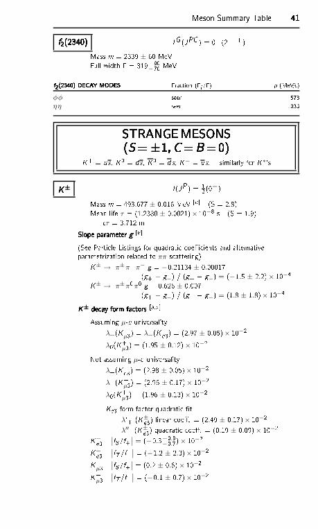
Meson Summary Table 41414141f2(2340)f2(2340)f2(2340)f2(2340) IG (JPC ) = 0+(2 + +)Mass m = 2339 ± 60 MeVFull width = 319+80−70 MeVf2(2340) DECAY MODESf2(2340) DECAY MODESf2(2340) DECAY MODESf2(2340) DECAY MODES Fra tion (i /) p (MeV/ )
φφ seen 573ηη seen 1033STRANGEMESONSSTRANGEMESONSSTRANGEMESONSSTRANGEMESONS(S= ±1,C=B=0)(S= ±1,C=B=0)(S= ±1,C=B=0)(S= ±1,C=B=0)K+ = us , K0 = ds , K0 = d s, K− = u s, similarly for K∗'sK±K±K±K± I (JP ) = 12 (0−)Mass m = 493.677 ± 0.016 MeV [u (S = 2.8)Mean life τ = (1.2380 ± 0.0021)× 10−8 s (S = 1.9) τ = 3.712 mSlope parameter gSlope parameter gSlope parameter gSlope parameter g [v (See Parti le Listings for quadrati oeÆ ients and alternativeparametrization related to ππ s attering)K± → π±π+π− g = −0.21134 ± 0.00017(g+ − g−) / (g+ + g−) = (−1.5 ± 2.2)× 10−4K± → π±π0π0 g = 0.626 ± 0.007(g+ − g−) / (g+ + g−) = (1.8 ± 1.8)× 10−4K± de ay form fa torsK± de ay form fa torsK± de ay form fa torsK± de ay form fa tors [a,x Assuming µ-e universality
λ+(K+µ3) = λ+(K+e3) = (2.97 ± 0.05)× 10−2
λ0(K+µ3) = (1.95 ± 0.12)× 10−2Not assuming µ-e universality
λ+(K+e3) = (2.98 ± 0.05)× 10−2λ+(K+
µ3) = (2.96 ± 0.17)× 10−2λ0(K+
µ3) = (1.96 ± 0.13)× 10−2Ke3 form fa tor quadrati tλ'+ (K±e3) linear oe. = (2.49 ± 0.17)× 10−2λ′′+(K±e3) quadrati oe. = (0.19 ± 0.09)× 10−2K+e3 ∣
∣fS/f+∣
∣ = (−0.3+0.8−0.7)× 10−2K+e3 ∣
∣fT /f+∣
∣ = (−1.2 ± 2.3)× 10−2K+µ3 ∣
∣fS/f+∣
∣ = (0.2 ± 0.6)× 10−2K+µ3 ∣
∣fT /f+∣
∣ = (−0.1 ± 0.7)× 10−2
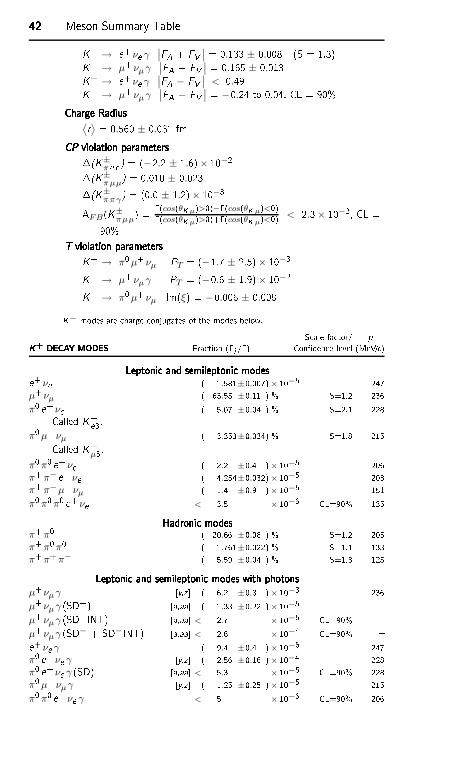
42424242 Meson Summary TableK+ → e+ νe γ∣
∣FA + FV ∣
∣ = 0.133 ± 0.008 (S = 1.3)K+ → µ+ νµ γ∣
∣FA + FV ∣
∣ = 0.165 ± 0.013K+ → e+ νe γ∣
∣FA − FV ∣
∣ < 0.49K+ → µ+ νµ γ∣
∣FA − FV ∣
∣ = −0.24 to 0.04, CL = 90%Charge RadiusCharge RadiusCharge RadiusCharge Radius⟨r⟩ = 0.560 ± 0.031 fmCP violation parametersCP violation parametersCP violation parametersCP violation parameters(K±
π e e ) = (−2.2 ± 1.6)× 10−2(K±πµµ) = 0.010 ± 0.023(K±ππγ) = (0.0 ± 1.2)× 10−3AFB(K±
πµµ) = (cos(θK µ)>0)−(cos(θK µ)<0)(cos(θK µ)>0)+(cos(θK µ)<0) < 2.3× 10⁻², CL =90%T violation parametersT violation parametersT violation parametersT violation parametersK+ → π0µ+ νµ PT = (−1.7 ± 2.5)× 10−3K+ → µ+ νµ γ PT = (−0.6 ± 1.9)× 10−2K+ → π0µ+ νµ Im(ξ) = −0.006 ± 0.008K− modes are harge onjugates of the modes below. S ale fa tor/ pK+ DECAY MODESK+ DECAY MODESK+ DECAY MODESK+ DECAY MODES Fra tion (i /) Conden e level (MeV/ )Leptoni and semileptoni modesLeptoni and semileptoni modesLeptoni and semileptoni modesLeptoni and semileptoni modese+ νe ( 1.581±0.007)× 10−5 247µ+νµ ( 63.55 ±0.11 ) % S=1.2 236π0 e+ νe ( 5.07 ±0.04 ) % S=2.1 228Called K+e3.π0µ+ νµ ( 3.353±0.034) % S=1.8 215Called K+
µ3.π0π0 e+ νe ( 2.2 ±0.4 )× 10−5 206π+π− e+ νe ( 4.254±0.032)× 10−5 203π+π−µ+ νµ ( 1.4 ±0.9 )× 10−5 151π0π0π0 e+ νe < 3.5 × 10⁻⁶ CL=90% 135Hadroni modesHadroni modesHadroni modesHadroni modesπ+π0 ( 20.66 ±0.08 ) % S=1.2 205π+π0π0 ( 1.761±0.022) % S=1.1 133π+π+π− ( 5.59 ±0.04 ) % S=1.3 125Leptoni and semileptoni modes with photonsLeptoni and semileptoni modes with photonsLeptoni and semileptoni modes with photonsLeptoni and semileptoni modes with photonsµ+νµ γ [y,z ( 6.2 ±0.8 )× 10−3 236µ+νµ γ (SD+) [a,aa ( 1.33 ±0.22 )× 10−5 µ+νµ γ (SD+INT) [a,aa < 2.7 × 10⁻⁵ CL=90% µ+νµ γ (SD− + SD−INT) [a,aa < 2.6 × 10⁻⁴ CL=90% e+ νe γ ( 9.4 ±0.4 )× 10−6 247π0 e+ νe γ [y,z ( 2.56 ±0.16 )× 10−4 228π0 e+ νe γ (SD) [a,aa < 5.3 × 10⁻⁵ CL=90% 228π0µ+ νµγ [y,z ( 1.25 ±0.25 )× 10−5 215π0π0 e+ νe γ < 5 × 10⁻⁶ CL=90% 206
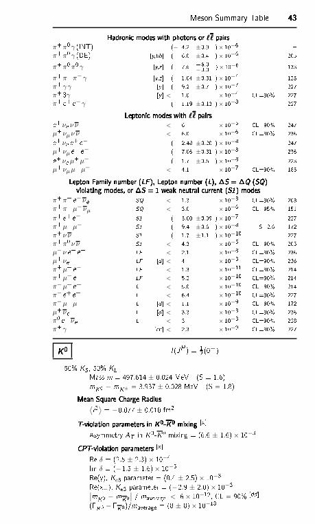
Meson Summary Table 43434343Hadroni modes with photons or ℓℓ pairsHadroni modes with photons or ℓℓ pairsHadroni modes with photons or ℓℓ pairsHadroni modes with photons or ℓℓ pairsπ+π0 γ (INT) (− 4.2 ±0.9 )× 10−6 π+π0 γ (DE) [y,bb ( 6.0 ±0.4 )× 10−6 205π+π0π0 γ [y,z ( 7.6 +6.0
−3.0 )× 10−6 133π+π+π− γ [y,z ( 1.04 ±0.31 )× 10−4 125π+ γ γ [y ( 9.2 ±0.7 )× 10−7 227π+ 3γ [y < 1.0 × 10⁻⁴ CL=90% 227π+ e+ e− γ ( 1.19 ±0.13 )× 10−8 227Leptoni modes with ℓℓ pairsLeptoni modes with ℓℓ pairsLeptoni modes with ℓℓ pairsLeptoni modes with ℓℓ pairse+ νe ν ν < 6 × 10⁻⁵ CL=90% 247µ+νµ ν ν < 6.0 × 10⁻⁶ CL=90% 236e+ νe e+ e− ( 2.48 ±0.20 )× 10−8 247µ+νµ e+ e− ( 7.06 ±0.31 )× 10−8 236e+ νe µ+µ− ( 1.7 ±0.5 )× 10−8 223µ+νµ µ+µ− < 4.1 × 10⁻⁷ CL=90% 185Lepton Family number (LF ), Lepton number (L), S = Q (SQ)Lepton Family number (LF ), Lepton number (L), S = Q (SQ)Lepton Family number (LF ), Lepton number (L), S = Q (SQ)Lepton Family number (LF ), Lepton number (L), S = Q (SQ)violating modes, or S = 1 weak neutral urrent (S1) modesviolating modes, or S = 1 weak neutral urrent (S1) modesviolating modes, or S = 1 weak neutral urrent (S1) modesviolating modes, or S = 1 weak neutral urrent (S1) modesπ+π+ e− νe SQ < 1.3 × 10⁻⁸ CL=90% 203π+π+µ− νµ SQ < 3.0 × 10⁻⁶ CL=95% 151π+ e+ e− S1 ( 3.00 ±0.09 )× 10−7 227π+µ+µ− S1 ( 9.4 ±0.6 )× 10−8 S=2.6 172π+ ν ν S1 ( 1.7 ±1.1 )× 10−10 227π+π0 ν ν S1 < 4.3 × 10⁻⁵ CL=90% 205µ−ν e+ e+ LF < 2.1 × 10⁻⁸ CL=90% 236µ+νe LF [d < 4 × 10⁻³ CL=90% 236π+µ+ e− LF < 1.3 × 10⁻¹¹ CL=90% 214π+µ− e+ LF < 5.2 × 10⁻¹⁰ CL=90% 214π−µ+ e+ L < 5.0 × 10⁻¹⁰ CL=90% 214π− e+ e+ L < 6.4 × 10⁻¹⁰ CL=90% 227π−µ+µ+ L [d < 1.1 × 10⁻⁹ CL=90% 172µ+νe L [d < 3.3 × 10⁻³ CL=90% 236π0 e+ νe L < 3 × 10⁻³ CL=90% 228π+ γ [ < 2.3 × 10⁻⁹ CL=90% 227K 0K 0K 0K 0 I (JP ) = 12 (0−)50% KS , 50% KLMass m = 497.614 ± 0.024 MeV (S = 1.6)mK0 − mK± = 3.937 ± 0.028 MeV (S = 1.8)Mean Square Charge RadiusMean Square Charge RadiusMean Square Charge RadiusMean Square Charge Radius
⟨r2⟩ = −0.077 ± 0.010 fm2T-violation parameters in K0-K0 mixingT-violation parameters in K0-K0 mixingT-violation parameters in K0-K0 mixingT-violation parameters in K0-K0 mixing [x Asymmetry AT in K0-K0 mixing = (6.6 ± 1.6)× 10−3CPT-violation parametersCPT-violation parametersCPT-violation parametersCPT-violation parameters [x Re δ = (2.5 ± 2.3)× 10−4Im δ = (−1.5 ± 1.6)× 10−5Re(y), Ke3 parameter = (0.4 ± 2.5)× 10−3Re(x−), Ke3 parameter = (−2.9 ± 2.0)× 10−3∣
∣mK0 − mK0∣∣ / maverage < 6× 10⁻¹⁹, CL = 90% [dd(K0 − K0)/maverage = (8 ± 8)× 10−18
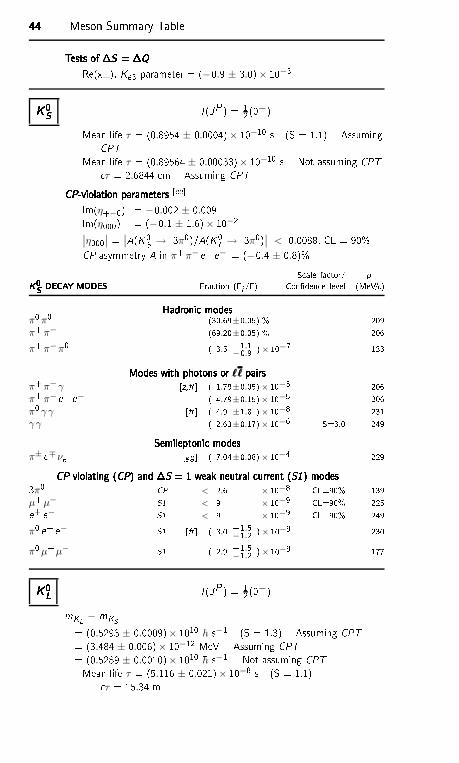
44444444 Meson Summary TableTests of S = QTests of S = QTests of S = QTests of S = QRe(x+), Ke3 parameter = (−0.9 ± 3.0)× 10−3K 0SK 0SK 0SK 0S I (JP ) = 12 (0−)Mean life τ = (0.8954 ± 0.0004)× 10−10 s (S = 1.1) AssumingCPTMean life τ = (0.89564 ± 0.00033)× 10−10 s Not assuming CPT τ = 2.6844 m Assuming CPTCP-violation parametersCP-violation parametersCP-violation parametersCP-violation parameters [eeIm(η+−0) = −0.002 ± 0.009Im(η000) = (−0.1 ± 1.6)× 10−2∣
∣η000∣∣ = ∣
∣A(K0S → 3π0)/A(K0L → 3π0)∣∣ < 0.0088, CL = 90%CP asymmetry A in π+π− e+ e− = (−0.4 ± 0.8)%S ale fa tor/ pK0S DECAY MODESK0S DECAY MODESK0S DECAY MODESK0S DECAY MODES Fra tion (i /) Conden e level (MeV/ )Hadroni modesHadroni modesHadroni modesHadroni modesπ0π0 (30.69±0.05) % 209π+π− (69.20±0.05) % 206π+π−π0 ( 3.5 +1.1
−0.9 )× 10−7 133Modes with photons or ℓℓ pairsModes with photons or ℓℓ pairsModes with photons or ℓℓ pairsModes with photons or ℓℓ pairsπ+π−γ [z, ( 1.79±0.05)× 10−3 206π+π− e+ e− ( 4.79±0.15)× 10−5 206π0 γ γ [ ( 4.9 ±1.8 )× 10−8 231γ γ ( 2.63±0.17)× 10−6 S=3.0 249Semileptoni modesSemileptoni modesSemileptoni modesSemileptoni modesπ± e∓νe [gg ( 7.04±0.08)× 10−4 229CP violating (CP) and S = 1 weak neutral urrent (S1) modesCP violating (CP) and S = 1 weak neutral urrent (S1) modesCP violating (CP) and S = 1 weak neutral urrent (S1) modesCP violating (CP) and S = 1 weak neutral urrent (S1) modes3π0 CP < 2.6 × 10⁻⁸ CL=90% 139µ+µ− S1 < 9 × 10⁻⁹ CL=90% 225e+ e− S1 < 9 × 10⁻⁹ CL=90% 249π0 e+ e− S1 [ ( 3.0 +1.5
−1.2 )× 10−9 230π0µ+µ− S1 ( 2.9 +1.5
−1.2 )× 10−9 177K 0LK 0LK 0LK 0L I (JP ) = 12 (0−)mKL − mKS= (0.5293 ± 0.0009)× 1010 h s−1 (S = 1.3) Assuming CPT= (3.484 ± 0.006)× 10−12 MeV Assuming CPT= (0.5289 ± 0.0010)× 1010 h s−1 Not assuming CPTMean life τ = (5.116 ± 0.021)× 10−8 s (S = 1.1) τ = 15.34 m
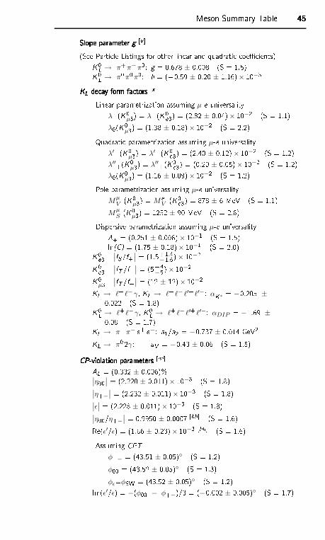
Meson Summary Table 45454545Slope parameter gSlope parameter gSlope parameter gSlope parameter g [v (See Parti le Listings for other linear and quadrati oeÆ ients)K0L → π+π−π0: g = 0.678 ± 0.008 (S = 1.5)K0L → π0π0π0: h = (+0.59 ± 0.20 ± 1.16)× 10−3KL de ay form fa torsKL de ay form fa torsKL de ay form fa torsKL de ay form fa tors [x Linear parametrization assuming µ-e universalityλ+(K0
µ3) = λ+(K0e3) = (2.82 ± 0.04)× 10−2 (S = 1.1)λ0(K0
µ3) = (1.38 ± 0.18)× 10−2 (S = 2.2)Quadrati parametrization assuming µ-e universalityλ′+(K0
µ3) = λ′+(K0e3) = (2.40 ± 0.12)× 10−2 (S = 1.2)λ′′+(K0
µ3) = λ′′+(K0e3) = (0.20 ± 0.05)× 10−2 (S = 1.2)λ0(K0
µ3) = (1.16 ± 0.09)× 10−2 (S = 1.2)Pole parametrization assuming µ-e universalityM
µV (K0
µ3) = M eV (K0e3) = 878 ± 6 MeV (S = 1.1)
MµS (K0
µ3) = 1252 ± 90 MeV (S = 2.6)Dispersive parametrization assuming µ-e universality+ = (0.251 ± 0.006)× 10−1 (S = 1.5)ln(C) = (1.75 ± 0.18)× 10−1 (S = 2.0)K0e3 ∣
∣fS/f+∣
∣ = (1.5+1.4−1.6)× 10−2K0e3 ∣
∣fT /f+∣
∣ = (5+4−5)× 10−2K0
µ3 ∣
∣fT /f+∣
∣ = (12 ± 12)× 10−2KL → ℓ+ ℓ−γ, KL → ℓ+ ℓ− ℓ′+ ℓ′−: αK∗ = −0.205 ±0.022 (S = 1.8)K0L → ℓ+ ℓ−γ, K0L → ℓ+ ℓ− ℓ′+ ℓ′−: αDIP = −1.69 ±0.08 (S = 1.7)KL → π+π− e+ e−: a1/a2 = −0.737 ± 0.014 GeV2KL → π0 2γ: aV = −0.43 ± 0.06 (S = 1.5)CP-violation parametersCP-violation parametersCP-violation parametersCP-violation parameters [eeAL = (0.332 ± 0.006)%∣
∣η00∣∣ = (2.220 ± 0.011)× 10−3 (S = 1.8)∣
∣η+−∣
∣ = (2.232 ± 0.011)× 10−3 (S = 1.8)∣
∣ǫ∣
∣ = (2.228 ± 0.011)× 10−3 (S = 1.8)∣
∣η00/η+−∣
∣ = 0.9950 ± 0.0007 [hh (S = 1.6)Re(ǫ′/ǫ) = (1.66 ± 0.23)× 10−3 [hh (S = 1.6)Assuming CPTφ+− = (43.51 ± 0.05) (S = 1.2)φ00 = (43.52 ± 0.05) (S = 1.3)φǫ=φSW = (43.52 ± 0.05) (S = 1.2)Im(ǫ′/ǫ) = −(φ00 − φ+−)/3 = (−0.002 ± 0.005) (S = 1.7)
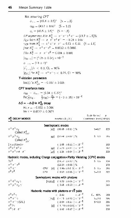
46464646 Meson Summary TableNot assuming CPTφ+− = (43.4 ± 0.5) (S = 1.2)φ00 = (43.7 ± 0.6) (S = 1.2)φǫ = (43.5 ± 0.5) (S = 1.3)CP asymmetry A in K0L → π+π− e+ e− = (13.7 ± 1.5)%
βCP from K0L → e+ e− e+ e− = −0.19 ± 0.07γCP from K0L → e+ e− e+ e− = 0.01 ± 0.11 (S = 1.6)j for K0L → π+π−π0 = 0.0012 ± 0.0008f for K0L → π+π−π0 = 0.004 ± 0.006∣
∣η+−γ
∣
∣ = (2.35 ± 0.07)× 10−3φ+−γ = (44 ± 4)∣
∣ǫ′+−γ
∣
∣/ǫ < 0.3, CL = 90%∣
∣gE1∣∣ for K0L → π+π− γ < 0.21, CL = 90%T-violation parametersT-violation parametersT-violation parametersT-violation parametersIm(ξ) in K0µ3 = −0.007 ± 0.026CPT invarian e testsCPT invarian e testsCPT invarian e testsCPT invarian e tests
φ00 − φ+− = (0.34 ± 0.32)Re(23η+− + 13η00)−AL2 = (−3 ± 35)× 10−6S = −Q in K0ℓ3 de ayS = −Q in K0ℓ3 de ayS = −Q in K0ℓ3 de ayS = −Q in K0ℓ3 de ayRe x = −0.002 ± 0.006Im x = 0.0012 ± 0.0021 S ale fa tor/ pK0L DECAY MODESK0L DECAY MODESK0L DECAY MODESK0L DECAY MODES Fra tion (i /) Conden e level (MeV/ )Semileptoni modesSemileptoni modesSemileptoni modesSemileptoni modes
π± e∓νe [gg (40.55 ±0.11 ) % S=1.7 229Called K0e3.π±µ∓νµ [gg (27.04 ±0.07 ) % S=1.1 216Called K0
µ3.(πµatom)ν ( 1.05 ±0.11 )× 10−7 188π0π± e∓ν [gg ( 5.20 ±0.11 )× 10−5 207π± e∓ν e+ e− [gg ( 1.26 ±0.04 )× 10−5 229Hadroni modes, in luding Charge onjugation×Parity Violating (CPV) modesHadroni modes, in luding Charge onjugation×Parity Violating (CPV) modesHadroni modes, in luding Charge onjugation×Parity Violating (CPV) modesHadroni modes, in luding Charge onjugation×Parity Violating (CPV) modes3π0 (19.52 ±0.12 ) % S=1.6 139π+π−π0 (12.54 ±0.05 ) % 133π+π− CPV [ii ( 1.967±0.010)× 10−3 S=1.5 206π0π0 CPV ( 8.64 ±0.06 )× 10−4 S=1.8 209Semileptoni modes with photonsSemileptoni modes with photonsSemileptoni modes with photonsSemileptoni modes with photonsπ± e∓νe γ [z,gg,jj ( 3.79 ±0.06 )× 10−3 229π±µ∓νµ γ ( 5.65 ±0.23 )× 10−4 216Hadroni modes with photons or ℓℓ pairsHadroni modes with photons or ℓℓ pairsHadroni modes with photons or ℓℓ pairsHadroni modes with photons or ℓℓ pairsπ0π0 γ < 2.43 × 10⁻⁷ CL=90% 209π+π−γ [z,jj ( 4.15 ±0.15 )× 10−5 S=2.8 206π+π−γ (DE) ( 2.84 ±0.11 )× 10−5 S=2.0 206π0 2γ [jj ( 1.273±0.033)× 10−6 231π0 γ e+ e− ( 1.62 ±0.17 )× 10−8 230
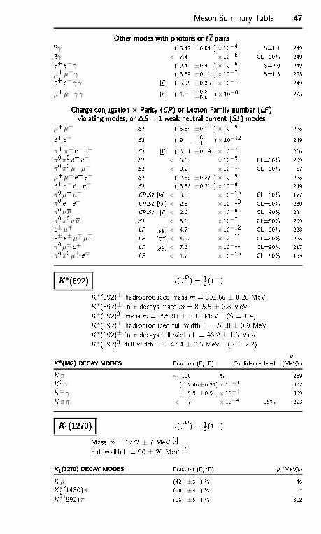
Meson Summary Table 47474747Other modes with photons or ℓℓ pairsOther modes with photons or ℓℓ pairsOther modes with photons or ℓℓ pairsOther modes with photons or ℓℓ pairs2γ ( 5.47 ±0.04 )× 10−4 S=1.1 2493γ < 7.4 × 10⁻⁸ CL=90% 249e+ e−γ ( 9.4 ±0.4 )× 10−6 S=2.0 249µ+µ− γ ( 3.59 ±0.11 )× 10−7 S=1.3 225e+ e−γ γ [jj ( 5.95 ±0.33 )× 10−7 249µ+µ− γ γ [jj ( 1.0 +0.8
−0.6 )× 10−8 225Charge onjugation × Parity (CP) or Lepton Family number (LF )Charge onjugation × Parity (CP) or Lepton Family number (LF )Charge onjugation × Parity (CP) or Lepton Family number (LF )Charge onjugation × Parity (CP) or Lepton Family number (LF )violating modes, or S = 1 weak neutral urrent (S1) modesviolating modes, or S = 1 weak neutral urrent (S1) modesviolating modes, or S = 1 weak neutral urrent (S1) modesviolating modes, or S = 1 weak neutral urrent (S1) modesµ+µ− S1 ( 6.84 ±0.11 )× 10−9 225e+ e− S1 ( 9 +6
−4 )× 10−12 249π+π− e+ e− S1 [jj ( 3.11 ±0.19 )× 10−7 206π0π0 e+ e− S1 < 6.6 × 10⁻⁹ CL=90% 209π0π0µ+µ− S1 < 9.2 × 10⁻¹¹ CL=90% 57µ+µ− e+ e− S1 ( 2.69 ±0.27 )× 10−9 225e+ e− e+ e− S1 ( 3.56 ±0.21 )× 10−8 249π0µ+µ− CP,S1 [kk < 3.8 × 10⁻¹⁰ CL=90% 177π0 e+ e− CP,S1 [kk < 2.8 × 10⁻¹⁰ CL=90% 230π0 ν ν CP,S1 [ll < 2.6 × 10⁻⁸ CL=90% 231π0π0 ν ν S1 < 8.1 × 10⁻⁷ CL=90% 209e±µ∓ LF [gg < 4.7 × 10⁻¹² CL=90% 238e± e±µ∓µ∓ LF [gg < 4.12 × 10⁻¹¹ CL=90% 225π0µ± e∓ LF [gg < 7.6 × 10⁻¹¹ CL=90% 217π0π0µ± e∓ LF < 1.7 × 10⁻¹⁰ CL=90% 159K ∗(892)K ∗(892)K ∗(892)K ∗(892) I (JP ) = 12 (1−)K∗(892)± hadroprodu ed mass m = 891.66 ± 0.26 MeVK∗(892)± in τ de ays mass m = 895.5 ± 0.8 MeVK∗(892)0 mass m = 895.81 ± 0.19 MeV (S = 1.4)K∗(892)± hadroprodu ed full width = 50.8 ± 0.9 MeVK∗(892)± in τ de ays full width = 46.2 ± 1.3 MeVK∗(892)0 full width = 47.4 ± 0.6 MeV (S = 2.2) pK∗(892) DECAY MODESK∗(892) DECAY MODESK∗(892) DECAY MODESK∗(892) DECAY MODES Fra tion (i /) Conden e level (MeV/ )K π ∼ 100 % 289K0γ ( 2.46±0.21)× 10−3 307K±γ ( 9.9 ±0.9 )× 10−4 309K ππ < 7 × 10⁻⁴ 95% 223K1(1270)K1(1270)K1(1270)K1(1270) I (JP ) = 12 (1+)Mass m = 1272 ± 7 MeV [lFull width = 90 ± 20 MeV [lK1(1270) DECAY MODESK1(1270) DECAY MODESK1(1270) DECAY MODESK1(1270) DECAY MODES Fra tion (i /) p (MeV/ )K ρ (42 ±6 ) % 46K∗0(1430)π (28 ±4 ) % †K∗(892)π (16 ±5 ) % 302
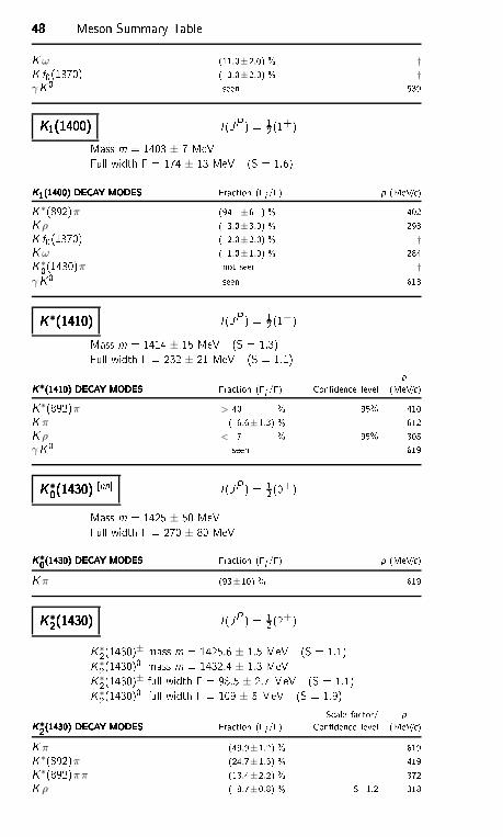
48484848 Meson Summary TableK ω (11.0±2.0) % †K f0(1370) ( 3.0±2.0) % †γK0 seen 539K1(1400)K1(1400)K1(1400)K1(1400) I (JP ) = 12 (1+)Mass m = 1403 ± 7 MeVFull width = 174 ± 13 MeV (S = 1.6)K1(1400) DECAY MODESK1(1400) DECAY MODESK1(1400) DECAY MODESK1(1400) DECAY MODES Fra tion (i /) p (MeV/ )K∗(892)π (94 ±6 ) % 402K ρ ( 3.0±3.0) % 293K f0(1370) ( 2.0±2.0) % †K ω ( 1.0±1.0) % 284K∗0(1430)π not seen †γK0 seen 613K ∗(1410)K ∗(1410)K ∗(1410)K ∗(1410) I (JP ) = 12 (1−)Mass m = 1414 ± 15 MeV (S = 1.3)Full width = 232 ± 21 MeV (S = 1.1) pK∗(1410) DECAY MODESK∗(1410) DECAY MODESK∗(1410) DECAY MODESK∗(1410) DECAY MODES Fra tion (i /) Conden e level (MeV/ )K∗(892)π > 40 % 95% 410K π ( 6.6±1.3) % 612K ρ < 7 % 95% 305γK0 seen 619K ∗0(1430)K ∗0(1430)K ∗0(1430)K ∗0(1430) [nn I (JP ) = 12 (0+)Mass m = 1425 ± 50 MeVFull width = 270 ± 80 MeVK∗0(1430) DECAY MODESK∗0(1430) DECAY MODESK∗0(1430) DECAY MODESK∗0(1430) DECAY MODES Fra tion (i /) p (MeV/ )K π (93±10) % 619K ∗2(1430)K ∗2(1430)K ∗2(1430)K ∗2(1430) I (JP ) = 12 (2+)K∗2(1430)± mass m = 1425.6 ± 1.5 MeV (S = 1.1)K∗2(1430)0 mass m = 1432.4 ± 1.3 MeVK∗2(1430)± full width = 98.5 ± 2.7 MeV (S = 1.1)K∗2(1430)0 full width = 109 ± 5 MeV (S = 1.9)S ale fa tor/ pK∗2(1430) DECAY MODESK∗2(1430) DECAY MODESK∗2(1430) DECAY MODESK∗2(1430) DECAY MODES Fra tion (i /) Conden e level (MeV/ )K π (49.9±1.2) % 619K∗(892)π (24.7±1.5) % 419K∗(892)ππ (13.4±2.2) % 372K ρ ( 8.7±0.8) % S=1.2 318
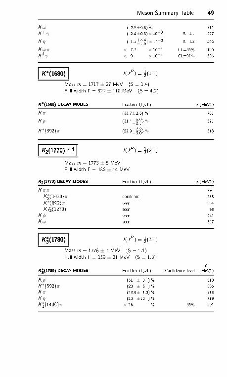
Meson Summary Table 49494949K ω ( 2.9±0.8) % 311K+γ ( 2.4±0.5)× 10−3 S=1.1 627K η ( 1.5+3.4−1.0)× 10−3 S=1.3 486K ωπ < 7.2 × 10⁻⁴ CL=95% 100K0γ < 9 × 10⁻⁴ CL=90% 626K ∗(1680)K ∗(1680)K ∗(1680)K ∗(1680) I (JP ) = 12 (1−)Mass m = 1717 ± 27 MeV (S = 1.4)Full width = 322 ± 110 MeV (S = 4.2)K∗(1680) DECAY MODESK∗(1680) DECAY MODESK∗(1680) DECAY MODESK∗(1680) DECAY MODES Fra tion (i /) p (MeV/ )K π (38.7±2.5) % 781K ρ (31.4+5.0
−2.1) % 571K∗(892)π (29.9+2.2−5.0) % 618K2(1770)K2(1770)K2(1770)K2(1770) [oo I (JP ) = 12 (2−)Mass m = 1773 ± 8 MeVFull width = 186 ± 14 MeVK2(1770) DECAY MODESK2(1770) DECAY MODESK2(1770) DECAY MODESK2(1770) DECAY MODES Fra tion (i /) p (MeV/ )K ππ 794K∗2(1430)π dominant 288K∗(892)π seen 654K f2(1270) seen 55K φ seen 441K ω seen 607K ∗3(1780)K ∗3(1780)K ∗3(1780)K ∗3(1780) I (JP ) = 12 (3−)Mass m = 1776 ± 7 MeV (S = 1.1)Full width = 159 ± 21 MeV (S = 1.3) pK∗3(1780) DECAY MODESK∗3(1780) DECAY MODESK∗3(1780) DECAY MODESK∗3(1780) DECAY MODES Fra tion (i /) Conden e level (MeV/ )K ρ (31 ± 9 ) % 613K∗(892)π (20 ± 5 ) % 656K π (18.8± 1.0) % 813K η (30 ±13 ) % 719K∗2(1430)π < 16 % 95% 291
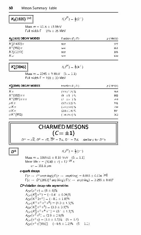
50505050 Meson Summary TableK2(1820)K2(1820)K2(1820)K2(1820) [pp I (JP ) = 12 (2−)Mass m = 1816 ± 13 MeVFull width = 276 ± 35 MeVK2(1820) DECAY MODESK2(1820) DECAY MODESK2(1820) DECAY MODESK2(1820) DECAY MODES Fra tion (i /) p (MeV/ )K∗2(1430)π seen 327K∗(892)π seen 681K f2(1270) seen 186K ω seen 638K ∗4(2045)K ∗4(2045)K ∗4(2045)K ∗4(2045) I (JP ) = 12 (4+)Mass m = 2045 ± 9 MeV (S = 1.1)Full width = 198 ± 30 MeVK∗4(2045) DECAY MODESK∗4(2045) DECAY MODESK∗4(2045) DECAY MODESK∗4(2045) DECAY MODES Fra tion (i /) p (MeV/ )K π (9.9±1.2) % 958K∗(892)ππ (9 ±5 ) % 802K∗(892)πππ (7 ±5 ) % 768ρK π (5.7±3.2) % 741ωK π (5.0±3.0) % 738φK π (2.8±1.4) % 594φK∗(892) (1.4±0.7) % 363CHARMEDMESONSCHARMEDMESONSCHARMEDMESONSCHARMEDMESONS(C= ±1)(C= ±1)(C= ±1)(C= ±1)D+ = d , D0 = u, D0 = u, D− = d, similarly for D∗'sD±D±D±D± I (JP ) = 12 (0−)Mass m = 1869.61 ± 0.10 MeV (S = 1.1)Mean life τ = (1040 ± 7)× 10−15 s τ = 311.8 µm -quark de ays -quark de ays -quark de ays -quark de ays( → ℓ+anything)/( → anything) = 0.096 ± 0.004 [qq( → D∗(2010)+ anything)/( → anything) = 0.255 ± 0.017CP-violation de ay-rate asymmetriesCP-violation de ay-rate asymmetriesCP-violation de ay-rate asymmetriesCP-violation de ay-rate asymmetriesACP (µ±ν) = (8 ± 8)%ACP (K0S π±) = (−0.41 ± 0.09)%ACP (K∓2π±) = (−0.1 ± 1.0)%ACP (K∓π±π±π0) = (1.0 ± 1.3)%ACP (K0S π±π0) = (0.3 ± 0.9)%ACP (K0S π±π+π−) = (0.1 ± 1.3)%ACP (π±π0) = (2.9 ± 2.9)%ACP (π± η) = (1.0 ± 1.5)% (S = 1.4)ACP (π± η′(958)) = (−0.5 ± 1.2)% (S = 1.1)
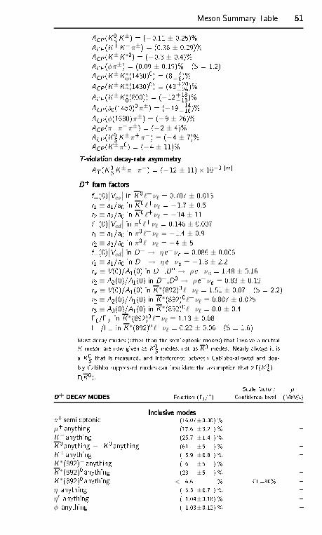
Meson Summary Table 51515151ACP (K0S K±) = (−0.11 ± 0.25)%ACP (K+K−π±) = (0.36 ± 0.29)%ACP (K±K∗0) = (−0.3 ± 0.4)%ACP (φπ±) = (0.09 ± 0.19)% (S = 1.2)ACP (K±K∗0(1430)0) = (8+7−6)%ACP (K±K∗2(1430)0) = (43+20−26)%ACP (K±K∗0(800)) = (−12+18−13)%ACP (a0(1450)0π±) = (−19+14−16)%ACP (φ(1680)π±) = (−9 ± 26)%ACP (π+π−π±) = (−2 ± 4)%ACP (K0S K±π+π−) = (−4 ± 7)%ACP (K±π0) = (−4 ± 11)%T-violation de ay-rate asymmetryT-violation de ay-rate asymmetryT-violation de ay-rate asymmetryT-violation de ay-rate asymmetryAT (K0S K±π+π−) = (−12 ± 11)× 10−3 [rr D+ form fa torsD+ form fa torsD+ form fa torsD+ form fa torsf+(0)∣∣Vcs
∣
∣ in K0 ℓ+νℓ = 0.707 ± 0.013r1 ≡ a1/a0 in K0 ℓ+νℓ = −1.7 ± 0.5r2 ≡ a2/a0 in K0 ℓ+νℓ = −14 ± 11f+(0)∣∣Vcd
∣
∣ in π0 ℓ+νℓ = 0.146 ± 0.007r1 ≡ a1/a0 in π0 ℓ+νℓ = −1.4 ± 0.9r2 ≡ a2/a0 in π0 ℓ+νℓ = −4 ± 5f+(0)∣∣Vcd
∣
∣ in D+ → ηe+ νe = 0.086 ± 0.006r1 ≡ a1/a0 in D+ → ηe+ νe = −1.8 ± 2.2rv ≡ V(0)/A1(0) in D+,D0 → ρe+ νe = 1.48 ± 0.16r2 ≡ A2(0)/A1(0) in D+,D0 → ρe+ νe = 0.83 ± 0.12rv ≡ V(0)/A1(0) in K∗(892)0 ℓ+νℓ = 1.51 ± 0.07 (S = 2.2)r2 ≡ A2(0)/A1(0) in K∗(892)0 ℓ+νℓ = 0.807 ± 0.025r3 ≡ A3(0)/A1(0) in K∗(892)0 ℓ+νℓ = 0.0 ± 0.4L/T in K∗(892)0 ℓ+νℓ = 1.13 ± 0.08+/− in K∗(892)0 ℓ+νℓ = 0.22 ± 0.06 (S = 1.6)Most de ay modes (other than the semileptoni modes) that involve a neutralK meson are now given as K0S modes, not as K0 modes. Nearly always it isa K0S that is measured, and interferen e between Cabibbo-allowed and dou-bly Cabibbo-suppressed modes an invalidate the assumption that 2 (K0S ) =(K0). S ale fa tor/ pD+ DECAY MODESD+ DECAY MODESD+ DECAY MODESD+ DECAY MODES Fra tion (i /) Conden e level (MeV/ )In lusive modesIn lusive modesIn lusive modesIn lusive modese+ semileptoni (16.07±0.30) % µ+ anything (17.6 ±3.2 ) % K− anything (25.7 ±1.4 ) % K0anything + K0 anything (61 ±5 ) % K+ anything ( 5.9 ±0.8 ) % K∗(892)− anything ( 6 ±5 ) % K∗(892)0 anything (23 ±5 ) % K∗(892)0 anything < 6.6 % CL=90% η anything ( 6.3 ±0.7 ) % η′ anything ( 1.04±0.18) % φ anything ( 1.03±0.12) %
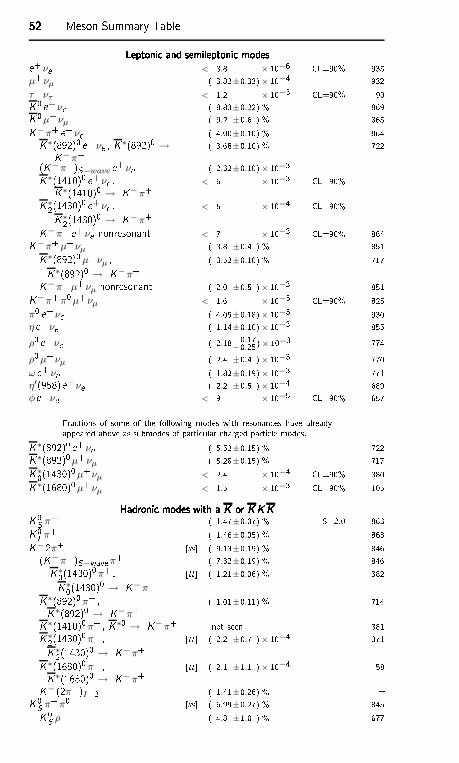
52525252 Meson Summary TableLeptoni and semileptoni modesLeptoni and semileptoni modesLeptoni and semileptoni modesLeptoni and semileptoni modese+ νe < 8.8 × 10⁻⁶ CL=90% 935µ+νµ ( 3.82±0.33)× 10−4 932τ+ ντ < 1.2 × 10⁻³ CL=90% 90K0 e+ νe ( 8.83±0.22) % 869K0µ+ νµ ( 9.2 ±0.6 ) % 865K−π+ e+νe ( 4.00±0.10) % 864K∗(892)0 e+νe , K∗(892)0 →K−π+ ( 3.68±0.10) % 722(K−π+)S−wave e+νe ( 2.32±0.10)× 10−3 K∗(1410)0 e+νe ,K∗(1410)0 → K−π+ < 6 × 10⁻³ CL=90% K∗2(1430)0 e+νe ,K∗2(1430)0 → K−π+ < 5 × 10⁻⁴ CL=90% K−π+ e+νe nonresonant < 7 × 10⁻³ CL=90% 864K−π+µ+νµ ( 3.8 ±0.4 ) % 851K∗(892)0µ+νµ ,K∗(892)0 → K−π+ ( 3.52±0.10) % 717K−π+µ+νµ nonresonant ( 2.0 ±0.5 )× 10−3 851K−π+π0µ+νµ < 1.6 × 10⁻³ CL=90% 825π0 e+ νe ( 4.05±0.18)× 10−3 930ηe+ νe ( 1.14±0.10)× 10−3 855ρ0 e+νe ( 2.18+0.17
−0.25)× 10−3 774ρ0µ+νµ ( 2.4 ±0.4 )× 10−3 770ω e+ νe ( 1.82±0.19)× 10−3 771η′(958)e+νe ( 2.2 ±0.5 )× 10−4 689φe+ νe < 9 × 10⁻⁵ CL=90% 657Fra tions of some of the following modes with resonan es have alreadyappeared above as submodes of parti ular harged-parti le modes.K∗(892)0 e+νe ( 5.52±0.15) % 722K∗(892)0µ+νµ ( 5.28±0.15) % 717K∗0(1430)0µ+νµ < 2.4 × 10⁻⁴ CL=90% 380K∗(1680)0µ+νµ < 1.5 × 10⁻³ CL=90% 105Hadroni modes with a K or K K KHadroni modes with a K or K K KHadroni modes with a K or K K KHadroni modes with a K or K K KK0S π+ ( 1.47±0.07) % S=2.0 863K0Lπ+ ( 1.46±0.05) % 863K−2π+ [ss ( 9.13±0.19) % 846(K−π+)S−waveπ+ ( 7.32±0.19) % 846K∗0(1430)0π+ ,K∗0(1430)0 → K−π+ [tt ( 1.21±0.06) % 382K∗(892)0π+ ,K∗(892)0 → K−π+ ( 1.01±0.11) % 714K∗(1410)0π+ , K∗0 → K−π+ not seen 381K∗2(1430)0π+ ,K∗2(1430)0 → K−π+ [tt ( 2.2 ±0.7 )× 10−4 371K∗(1680)0π+ ,K∗(1680)0 → K−π+ [tt ( 2.1 ±1.1 )× 10−4 58K− (2π+)I=2 ( 1.41±0.26) % K0S π+π0 [ss ( 6.99±0.27) % 845K0S ρ+ ( 4.8 ±1.0 ) % 677
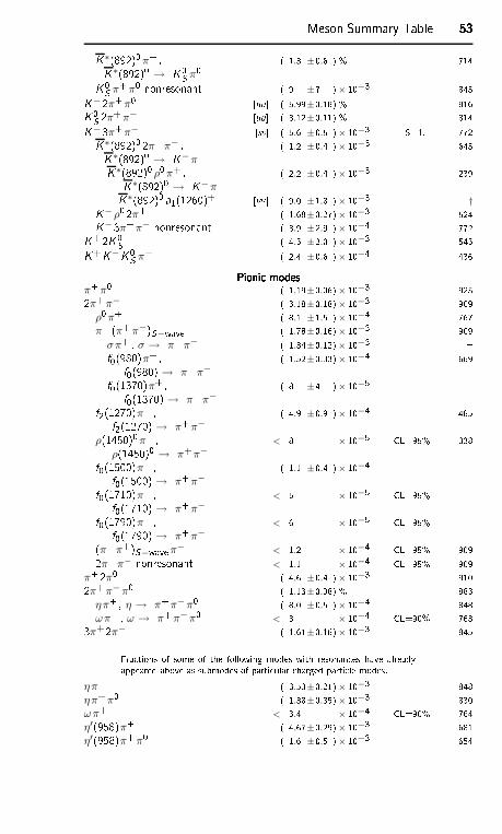
Meson Summary Table 53535353K∗(892)0π+ ,K∗(892)0 → K0S π0 ( 1.3 ±0.6 ) % 714K0S π+π0 nonresonant ( 9 ±7 )× 10−3 845K−2π+π0 [uu ( 5.99±0.18) % 816K0S 2π+π− [uu ( 3.12±0.11) % 814K−3π+π− [ss ( 5.6 ±0.5 )× 10−3 S=1.1 772K∗(892)0 2π+π− ,K∗(892)0 → K−π+ ( 1.2 ±0.4 )× 10−3 645K∗(892)0 ρ0π+ ,K∗(892)0 → K−π+ ( 2.2 ±0.4 )× 10−3 239K∗(892)0 a1(1260)+ [vv ( 9.0 ±1.8 )× 10−3 †K−ρ0 2π+ ( 1.68±0.27)× 10−3 524K−3π+π− nonresonant ( 3.9 ±2.9 )× 10−4 772K+2K0S ( 4.5 ±2.0 )× 10−3 545K+K−K0S π+ ( 2.4 ±0.6 )× 10−4 436Pioni modesPioni modesPioni modesPioni modesπ+π0 ( 1.19±0.06)× 10−3 9252π+π− ( 3.18±0.18)× 10−3 909
ρ0π+ ( 8.1 ±1.5 )× 10−4 767π+ (π+π−)S−wave ( 1.78±0.16)× 10−3 909
σπ+ , σ → π+π− ( 1.34±0.12)× 10−3 f0(980)π+ ,f0(980) → π+π−( 1.52±0.33)× 10−4 669f0(1370)π+ ,f0(1370) → π+π−( 8 ±4 )× 10−5 f2(1270)π+ ,f2(1270) → π+π−( 4.9 ±0.9 )× 10−4 485
ρ(1450)0π+ ,ρ(1450)0 → π+π−
< 8 × 10⁻⁵ CL=95% 338f0(1500)π+ ,f0(1500) → π+π−( 1.1 ±0.4 )× 10−4 f0(1710)π+ ,f0(1710) → π+π−
< 5 × 10⁻⁵ CL=95% f0(1790)π+ ,f0(1790) → π+π−< 6 × 10⁻⁵ CL=95% (π+π+)S−waveπ− < 1.2 × 10⁻⁴ CL=95% 9092π+π− nonresonant < 1.1 × 10⁻⁴ CL=95% 909
π+ 2π0 ( 4.6 ±0.4 )× 10−3 9102π+π−π0 ( 1.13±0.08) % 883ηπ+ , η → π+π−π0 ( 8.0 ±0.5 )× 10−4 848ωπ+ , ω → π+π−π0 < 3 × 10⁻⁴ CL=90% 7633π+2π− ( 1.61±0.16)× 10−3 845Fra tions of some of the following modes with resonan es have alreadyappeared above as submodes of parti ular harged-parti le modes.
ηπ+ ( 3.53±0.21)× 10−3 848ηπ+π0 ( 1.38±0.35)× 10−3 830ωπ+ < 3.4 × 10⁻⁴ CL=90% 764η′(958)π+ ( 4.67±0.29)× 10−3 681η′(958)π+π0 ( 1.6 ±0.5 )× 10−3 654
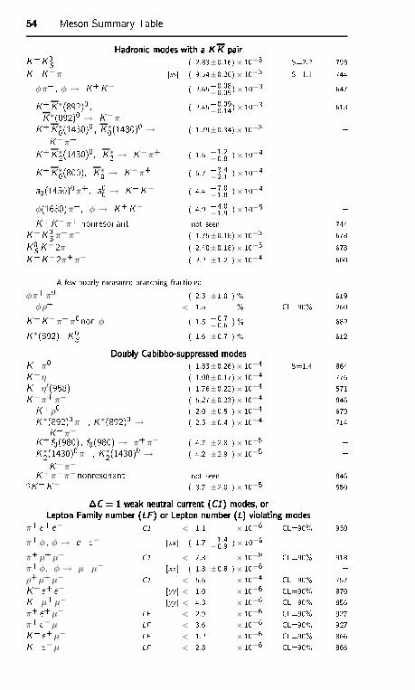
54545454 Meson Summary TableHadroni modes with a K K pairHadroni modes with a K K pairHadroni modes with a K K pairHadroni modes with a K K pairK+K0S ( 2.83±0.16)× 10−3 S=2.2 793K+K−π+ [ss ( 9.54±0.26)× 10−3 S=1.1 744φπ+ , φ → K+K− ( 2.65+0.08
−0.09)× 10−3 647K+K∗(892)0 ,K∗(892)0 → K−π+ ( 2.45+0.09−0.14)× 10−3 613K+K∗0(1430)0 , K∗0(1430)0 →K−π+ ( 1.79±0.34)× 10−3 K+K∗2(1430)0, K∗2 → K−π+ ( 1.6 +1.2−0.8 )× 10−4 K+K∗0(800), K∗0 → K−π+ ( 6.7 +3.4−2.1 )× 10−4 a0(1450)0π+, a00 → K+K− ( 4.4 +7.0−1.8 )× 10−4
φ(1680)π+, φ → K+K− ( 4.9 +4.0−1.9 )× 10−5 K+K−π+ nonresonant not seen 744K+K0S π+π− ( 1.75±0.18)× 10−3 678K0S K−2π+ ( 2.40±0.18)× 10−3 678K+K−2π+π− ( 2.2 ±1.2 )× 10−4 600A few poorly measured bran hing fra tions:
φπ+π0 ( 2.3 ±1.0 ) % 619φρ+ < 1.5 % CL=90% 260K+K−π+π0 non-φ ( 1.5 +0.7
−0.6 ) % 682K∗(892)+K0S ( 1.6 ±0.7 ) % 612Doubly Cabibbo-suppressed modesDoubly Cabibbo-suppressed modesDoubly Cabibbo-suppressed modesDoubly Cabibbo-suppressed modesK+π0 ( 1.83±0.26)× 10−4 S=1.4 864K+η ( 1.08±0.17)× 10−4 776K+η′(958) ( 1.76±0.22)× 10−4 571K+π+π− ( 5.27±0.23)× 10−4 846K+ρ0 ( 2.0 ±0.5 )× 10−4 679K∗(892)0π+ , K∗(892)0 →K+π−( 2.5 ±0.4 )× 10−4 714K+ f0(980), f0(980) → π+π− ( 4.7 ±2.8 )× 10−5 K∗2(1430)0π+ , K∗2(1430)0 →K+π−( 4.2 ±2.9 )× 10−5 K+π+π−nonresonant not seen 8462K+K− ( 8.7 ±2.0 )× 10−5 550C = 1 weak neutral urrent (C1) modes, orC = 1 weak neutral urrent (C1) modes, orC = 1 weak neutral urrent (C1) modes, orC = 1 weak neutral urrent (C1) modes, orLepton Family number (LF ) or Lepton number (L) violating modesLepton Family number (LF ) or Lepton number (L) violating modesLepton Family number (LF ) or Lepton number (L) violating modesLepton Family number (LF ) or Lepton number (L) violating modes
π+ e+ e− C1 < 1.1 × 10⁻⁶ CL=90% 930π+φ , φ → e+ e− [xx ( 1.7 +1.4
−0.9 )× 10−6 π+µ+µ− C1 < 7.3 × 10⁻⁸ CL=90% 918π+φ, φ → µ+µ− [xx ( 1.8 ±0.8 )× 10−6 ρ+µ+µ− C1 < 5.6 × 10⁻⁴ CL=90% 757K+ e+ e− [yy < 1.0 × 10⁻⁶ CL=90% 870K+µ+µ− [yy < 4.3 × 10⁻⁶ CL=90% 856π+ e+µ− LF < 2.9 × 10⁻⁶ CL=90% 927π+ e−µ+ LF < 3.6 × 10⁻⁶ CL=90% 927K+ e+µ− LF < 1.2 × 10⁻⁶ CL=90% 866K+ e−µ+ LF < 2.8 × 10⁻⁶ CL=90% 866
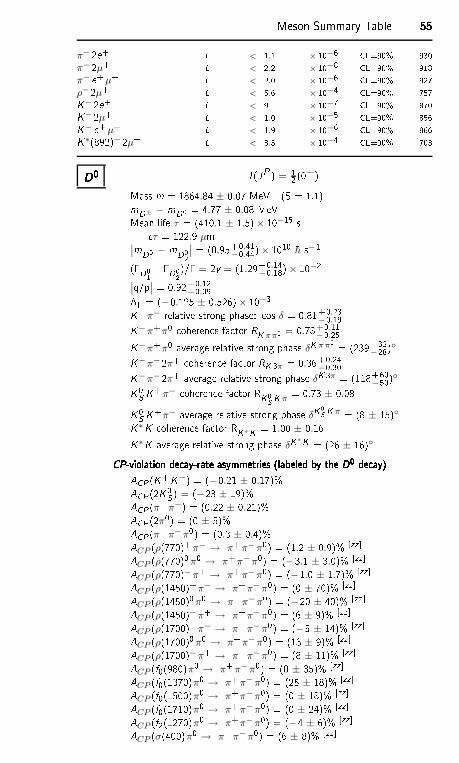
Meson Summary Table 55555555π− 2e+ L < 1.1 × 10⁻⁶ CL=90% 930π− 2µ+ L < 2.2 × 10⁻⁸ CL=90% 918π− e+µ+ L < 2.0 × 10⁻⁶ CL=90% 927ρ−2µ+ L < 5.6 × 10⁻⁴ CL=90% 757K−2e+ L < 9 × 10⁻⁷ CL=90% 870K−2µ+ L < 1.0 × 10⁻⁵ CL=90% 856K− e+µ+ L < 1.9 × 10⁻⁶ CL=90% 866K∗(892)− 2µ+ L < 8.5 × 10⁻⁴ CL=90% 703D0D0D0D0 I (JP ) = 12 (0−)Mass m = 1864.84 ± 0.07 MeV (S = 1.1)mD± − mD0 = 4.77 ± 0.08 MeVMean life τ = (410.1 ± 1.5)× 10−15 s τ = 122.9 µm
∣
∣mD01 − mD02∣∣ = (0.95+0.41−0.44)× 1010 h s−1(D01 D02)/ = 2y = (1.29+0.14
−0.18)× 10−2∣
∣q/p∣∣ = 0.92+0.12−0.09A = (−0.125 ± 0.526)× 10−3K+π− relative strong phase: os δ = 0.81+0.23
−0.19K−π+π0 oheren e fa tor RK ππ0 = 0.78+0.11−0.25K−π+π0 average relative strong phase δK ππ0 = (239+32
−28)K−π−2π+ oheren e fa tor RK 3π = 0.36+0.24−0.30K−π−2π+ average relative strong phase δK 3π = (118+60
−50)K0S K+π− oheren e fa tor RK0S K π= 0.73 ± 0.08K0S K+π− average relative strong phase δK0S K π = (8 ± 15)K∗K oheren e fa tor RK∗K = 1.00 ± 0.16K∗K average relative strong phase δK∗K = (26 ± 16)CP-violation de ay-rate asymmetries (labeled by the D0 de ay)CP-violation de ay-rate asymmetries (labeled by the D0 de ay)CP-violation de ay-rate asymmetries (labeled by the D0 de ay)CP-violation de ay-rate asymmetries (labeled by the D0 de ay)ACP (K+K−) = (−0.21 ± 0.17)%ACP (2K0S) = (−23 ± 19)%ACP (π+π−) = (0.22 ± 0.21)%ACP (2π0) = (0 ± 5)%ACP (π+π−π0) = (0.3 ± 0.4)%ACP (ρ(770)+π− → π+π−π0) = (1.2 ± 0.9)% [zz ACP (ρ(770)0π0 → π+π−π0) = (−3.1 ± 3.0)% [zz ACP (ρ(770)−π+ → π+π−π0) = (−1.0 ± 1.7)% [zz ACP (ρ(1450)+π− → π+π−π0) = (0 ± 70)% [zz ACP (ρ(1450)0π0 → π+π−π0) = (−20 ± 40)% [zz ACP (ρ(1450)−π+ → π+π−π0) = (6 ± 9)% [zz ACP (ρ(1700)+π− → π+π−π0) = (−5 ± 14)% [zz ACP (ρ(1700)0π0 → π+π−π0) = (13 ± 9)% [zz ACP (ρ(1700)−π+ → π+π−π0) = (8 ± 11)% [zz ACP (f0(980)π0 → π+π−π0) = (0 ± 35)% [zz ACP (f0(1370)π0 → π+π−π0) = (25 ± 18)% [zz ACP (f0(1500)π0 → π+π−π0) = (0 ± 18)% [zz ACP (f0(1710)π0 → π+π−π0) = (0 ± 24)% [zz ACP (f2(1270)π0 → π+π−π0) = (−4 ± 6)% [zz ACP (σ(400)π0 → π+π−π0) = (6 ± 8)% [zz
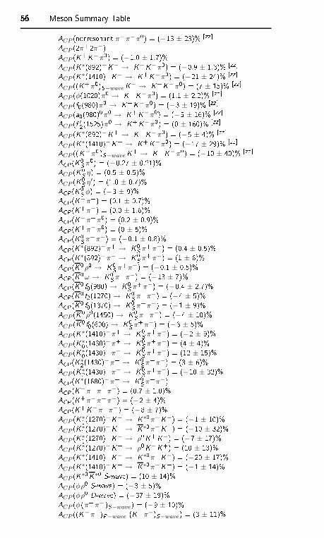
56565656 Meson Summary TableACP (nonresonant π+π−π0) = (−13 ± 23)% [zz ACP (2π+2π−)ACP (K+K−π0) = (−1.0 ± 1.7)%ACP (K∗(892)+K− → K+K−π0) = (−0.9 ± 1.3)% [zz ACP (K∗(1410)+K− → K+K−π0) = (−21 ± 24)% [zz ACP ((K+π0)S−waveK− → K+K−π0) = (7 ± 15)% [zz ACP (φ(1020)π0 → K+K−π0) = (1.1 ± 2.2)% [zz ACP (f0(980)π0 → K+K−π0) = (−3 ± 19)% [zz ACP (a0(980)0π0 → K+K−π0) = (−5 ± 16)% [zz ACP (f ′2(1525)π0 → K+K−π0) = (0 ± 160)% [zz ACP (K∗(892)−K+ → K+K−π0) = (−5 ± 4)% [zz ACP (K∗(1410)−K+ → K+K−π0) = (−17 ± 29)% [zz ACP ((K−π0 )S−waveK+ → K+K−π0) = (−10 ± 40)% [zz ACP (K0S π0) = (−0.27 ± 0.21)%ACP (K0S η) = (0.5 ± 0.5)%ACP (K0S η′) = (1.0 ± 0.7)%ACP (K0S φ) = (−3 ± 9)%ACP (K−π+) = (0.1 ± 0.7)%ACP (K+π−) = (0.0 ± 1.6)%ACP (K−π+π0) = (0.2 ± 0.9)%ACP (K+π−π0) = (0 ± 5)%ACP (K0S π+π−) = (−0.1 ± 0.8)%ACP (K∗(892)−π+ → K0S π+π−) = (0.4 ± 0.5)%ACP (K∗(892)+π− → K0S π+π−) = (1 ± 6)%ACP (K0ρ0 → K0S π+π−) = (−0.1 ± 0.5)%ACP (K0ω → K0S π+π−) = (−13 ± 7)%ACP (K0 f0(980) → K0S π+π−) = (−0.4 ± 2.7)%ACP (K0 f2(1270) → K0S π+π−) = (−4 ± 5)%ACP (K0 f0(1370) → K0S π+π−) = (−1 ± 9)%ACP (K0ρ0(1450) → K0S π+π−) = (−4 ± 10)%ACP (K0 f0(600) → K0S π+π−) = (−3 ± 5)%ACP (K∗(1410)−π+ → K0S π+π−) = (−2 ± 9)%ACP (K∗0(1430)−π+ → K0S π+π−) = (4 ± 4)%ACP (K∗0(1430)+π− → K0S π+π−) = (12 ± 15)%ACP (K∗2(1430)−π+ → K0S π+π−) = (3 ± 6)%ACP (K∗2(1430)+π− → K0S π+π−) = (−10 ± 32)%ACP (K∗(1680)−π+ → K0S π+π−)ACP (K−π+π+π−) = (0.7 ± 1.0)%ACP (K+π−π+π−) = (−2 ± 4)%ACP (K+K−π+π−) = (−8 ± 7)%ACP (K∗1(1270)+K− → K∗0π+K−) = (−1 ± 10)%ACP (K∗1(1270)−K+ → K∗0π−K+) = (−10 ± 32)%ACP (K∗1(1270)+K− → ρ0K+K−) = (−7 ± 17)%ACP (K∗1(1270)−K+ → ρ0K−K+) = (10 ± 13)%ACP (K∗(1410)+K− → K∗0π+K−) = (−20 ± 17)%ACP (K∗(1410)−K+ → K∗0π−K+) = (−1 ± 14)%ACP (K∗0K∗0 S-wave) = (10 ± 14)%ACP (φρ0 S-wave) = (−3 ± 5)%ACP (φρ0 D-wave) = (−37 ± 19)%ACP (φ(π+π− )S−wave) = (−9 ± 10)%ACP ((K−π+)P−wave (K+π−)S−wave) = (3 ± 11)%
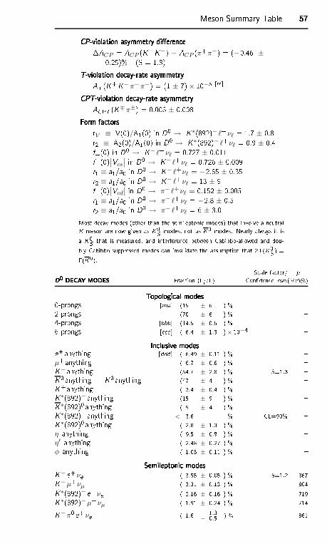
Meson Summary Table 57575757CP-violation asymmetry dieren eCP-violation asymmetry dieren eCP-violation asymmetry dieren eCP-violation asymmetry dieren eACP = ACP (K+K−) − ACP (π+π−) = (−0.46 ±0.25)% (S = 1.8)T-violation de ay-rate asymmetryT-violation de ay-rate asymmetryT-violation de ay-rate asymmetryT-violation de ay-rate asymmetryAT (K+K−π+π−) = (1 ± 7)× 10−3 [rr CPT-violation de ay-rate asymmetryCPT-violation de ay-rate asymmetryCPT-violation de ay-rate asymmetryCPT-violation de ay-rate asymmetryACPT (K∓π±) = 0.008 ± 0.008Form fa torsForm fa torsForm fa torsForm fa torsrV ≡ V(0)/A1(0) in D0 → K∗(892)− ℓ+νℓ = 1.7 ± 0.8r2 ≡ A2(0)/A1(0) in D0 → K∗(892)− ℓ+νℓ = 0.9 ± 0.4f+(0) in D0 → K− ℓ+νℓ = 0.727 ± 0.011f+(0)∣∣Vcs
∣
∣ in D0 → K− ℓ+νℓ = 0.726 ± 0.009r1 ≡ a1/a0 in D0 → K− ℓ+νℓ = −2.65 ± 0.35r2 ≡ a1/a0 in D0 → K− ℓ+νℓ = 13 ± 9f+(0)∣∣Vcd
∣
∣ in D0 → π− ℓ+νℓ = 0.152 ± 0.005r1 ≡ a1/a0 in D0 → π− ℓ+νℓ = −2.8 ± 0.5r2 ≡ a1/a0 in D0 → π− ℓ+νℓ = 6 ± 3.0Most de ay modes (other than the semileptoni modes) that involve a neutralK meson are now given as K0S modes, not as K0 modes. Nearly always it isa K0S that is measured, and interferen e between Cabibbo-allowed and dou-bly Cabibbo-suppressed modes an invalidate the assumption that 2 (K0S ) =(K0). S ale fa tor/ pD0 DECAY MODESD0 DECAY MODESD0 DECAY MODESD0 DECAY MODES Fra tion (i /) Conden e level(MeV/ )Topologi al modesTopologi al modesTopologi al modesTopologi al modes0-prongs [aaa (15 ± 6 ) % 2-prongs (70 ± 6 ) % 4-prongs [bbb (14.5 ± 0.5 ) % 6-prongs [ ( 6.4 ± 1.3 )× 10−4 In lusive modesIn lusive modesIn lusive modesIn lusive modese+ anything [ddd ( 6.49 ± 0.11 ) % µ+ anything ( 6.7 ± 0.6 ) % K− anything (54.7 ± 2.8 ) % S=1.3 K0anything + K0 anything (47 ± 4 ) % K+ anything ( 3.4 ± 0.4 ) % K∗(892)− anything (15 ± 9 ) % K∗(892)0 anything ( 9 ± 4 ) % K∗(892)+ anything < 3.6 % CL=90% K∗(892)0 anything ( 2.8 ± 1.3 ) % η anything ( 9.5 ± 0.9 ) % η′ anything ( 2.48 ± 0.27 ) % φ anything ( 1.05 ± 0.11 ) % Semileptoni modesSemileptoni modesSemileptoni modesSemileptoni modesK− e+ νe ( 3.55 ± 0.05 ) % S=1.2 867K−µ+νµ ( 3.31 ± 0.13 ) % 864K∗(892)− e+νe ( 2.16 ± 0.16 ) % 719K∗(892)−µ+νµ ( 1.91 ± 0.24 ) % 714K−π0 e+ νe ( 1.6 + 1.3
− 0.5 ) % 861
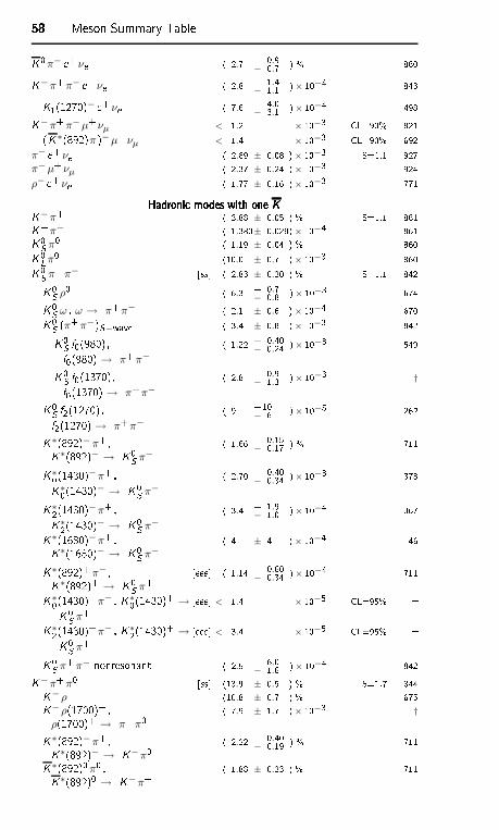
58585858 Meson Summary TableK0π− e+ νe ( 2.7 + 0.9− 0.7 ) % 860K−π+π− e+ νe ( 2.8 + 1.4− 1.1 )× 10−4 843K1(1270)− e+ νe ( 7.6 + 4.0− 3.1 )× 10−4 498K−π+π−µ+ νµ < 1.2 × 10⁻³ CL=90% 821(K∗(892)π )−µ+ νµ < 1.4 × 10⁻³ CL=90% 692
π− e+νe ( 2.89 ± 0.08 )× 10−3 S=1.1 927π−µ+νµ ( 2.37 ± 0.24 )× 10−3 924ρ− e+ νe ( 1.77 ± 0.16 )× 10−3 771Hadroni modes with one KHadroni modes with one KHadroni modes with one KHadroni modes with one KK−π+ ( 3.88 ± 0.05 ) % S=1.1 861K+π− ( 1.380± 0.028)× 10−4 861K0S π0 ( 1.19 ± 0.04 ) % 860K0Lπ0 (10.0 ± 0.7 )× 10−3 860K0S π+π− [ss ( 2.83 ± 0.20 ) % S=1.1 842K0S ρ0 ( 6.3 + 0.7
− 0.8 )× 10−3 674K0S ω , ω → π+π− ( 2.1 ± 0.6 )× 10−4 670K0S (π+π−)S−wave ( 3.4 ± 0.8 )× 10−3 842K0S f0(980),f0(980) → π+π−( 1.22 + 0.40
− 0.24 )× 10−3 549K0S f0(1370),f0(1370) → π+π−( 2.8 + 0.9
− 1.3 )× 10−3 †K0S f2(1270),f2(1270) → π+π−( 9 +10
− 6 )× 10−5 262K∗(892)−π+ ,K∗(892)− → K0S π−( 1.66 + 0.15
− 0.17 ) % 711K∗0(1430)−π+ ,K∗0(1430)− → K0S π−( 2.70 + 0.40
− 0.34 )× 10−3 378K∗2(1430)−π+ ,K∗2(1430)− → K0S π−( 3.4 + 1.9
− 1.0 )× 10−4 367K∗(1680)−π+ ,K∗(1680)− → K0S π−( 4 ± 4 )× 10−4 46K∗(892)+π− ,K∗(892)+ → K0S π+ [eee ( 1.14 + 0.60
− 0.34 )× 10−4 711K∗0(1430)+π− , K∗0(1430)+ →K0S π+ [eee < 1.4 × 10⁻⁵ CL=95% K∗2(1430)+π− , K∗2(1430)+ →K0S π+ [eee < 3.4 × 10⁻⁵ CL=95% K0S π+π− nonresonant ( 2.5 + 6.0− 1.6 )× 10−4 842K−π+π0 [ss (13.9 ± 0.5 ) % S=1.7 844K−ρ+ (10.8 ± 0.7 ) % 675K−ρ(1700)+ ,
ρ(1700)+ → π+π0 ( 7.9 ± 1.7 )× 10−3 †K∗(892)−π+ ,K∗(892)− → K−π0 ( 2.22 + 0.40− 0.19 ) % 711K∗(892)0π0 ,K∗(892)0 → K−π+ ( 1.88 ± 0.23 ) % 711
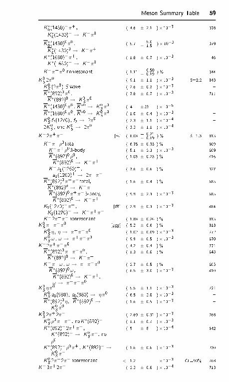
Meson Summary Table 59595959K∗0(1430)−π+ ,K∗0(1430)− → K−π0 ( 4.6 ± 2.1 )× 10−3 378K∗0(1430)0π0 ,K∗0(1430)0 → K−π+ ( 5.7 + 5.0− 1.5 )× 10−3 379K∗(1680)−π+ ,K∗(1680)− → K−π0 ( 1.8 ± 0.7 )× 10−3 46K−π+π0 nonresonant ( 1.11 + 0.50− 0.19 ) % 844K0S 2π0 ( 9.1 ± 1.1 )× 10−3 S=2.2 843K0S (2π0)-S-wave ( 2.6 ± 0.7 )× 10−3 K∗(892)0π0 ,K∗(892)0 → K0S π0 ( 7.8 ± 0.7 )× 10−3 711K∗(1430)0π0 , K∗0 → K0S π0 ( 4 ±23 )× 10−5 K∗(1680)0π0 , K∗0 → K0S π0 ( 1.0 ± 0.4 )× 10−3 K0S f2(1270), f2 → 2π0 ( 2.3 ± 1.1 )× 10−4 2K0S , one K0S → 2π0 ( 3.2 ± 1.1 )× 10−4 K−2π+π− [ss ( 8.08 + 0.21− 0.19 ) % S=1.3 813K−π+ ρ0 total ( 6.75 ± 0.33 ) % 609K−π+ ρ03-body ( 5.1 ± 2.3 )× 10−3 609K∗(892)0 ρ0 ,K∗(892)0 → K−π+ ( 1.05 ± 0.23 ) % 416K− a1(1260)+ ,a1(1260)+ → 2π+π−
( 3.6 ± 0.6 ) % 327K∗(892)0π+π− total,K∗(892)0 → K−π+ ( 1.6 ± 0.4 ) % 685K∗(892)0π+π−3-body,K∗(892)0 → K−π+ ( 9.9 ± 2.3 )× 10−3 685K1(1270)−π+ ,K1(1270)− → K−π+π−[f ( 2.9 ± 0.3 )× 10−3 484K−2π+π− nonresonant ( 1.88 ± 0.26 ) % 813K0S π+π−π0 [ggg ( 5.2 ± 0.6 ) % 813K0S η , η → π+π−π0 ( 1.02 ± 0.09 )× 10−3 772K0S ω , ω → π+π−π0 ( 9.9 ± 0.5 )× 10−3 670K−2π+π−π0 ( 4.2 ± 0.4 ) % 771K∗(892)0π+π−π0 ,K∗(892)0 → K−π+ ( 1.3 ± 0.6 ) % 643K−π+ω , ω → π+π−π0 ( 2.7 ± 0.5 ) % 605K∗(892)0ω ,K∗(892)0 → K−π+,
ω → π+π−π0 ( 6.5 ± 3.0 )× 10−3 410K0S ηπ0 ( 5.5 ± 1.1 )× 10−3 721K0S a0(980), a0(980) → ηπ0 ( 6.5 ± 2.0 )× 10−3 K∗(892)0 η, K∗(892)0 →K0S π0 ( 1.6 ± 0.5 )× 10−3 K0S 2π+2π− ( 2.69 ± 0.31 )× 10−3 768K0S ρ0π+π− , noK∗(892)− ( 1.1 ± 0.7 )× 10−3 K∗(892)− 2π+π− ,K∗(892)− → K0S π−, noρ0 ( 5 ± 8 )× 10−4 642K∗(892)− ρ0π+ , K∗(892)− →K0S π−
( 1.6 ± 0.6 )× 10−3 230K0S 2π+2π− nonresonant < 1.2 × 10⁻³ CL=90% 768K−3π+2π− ( 2.2 ± 0.6 )× 10−4 713
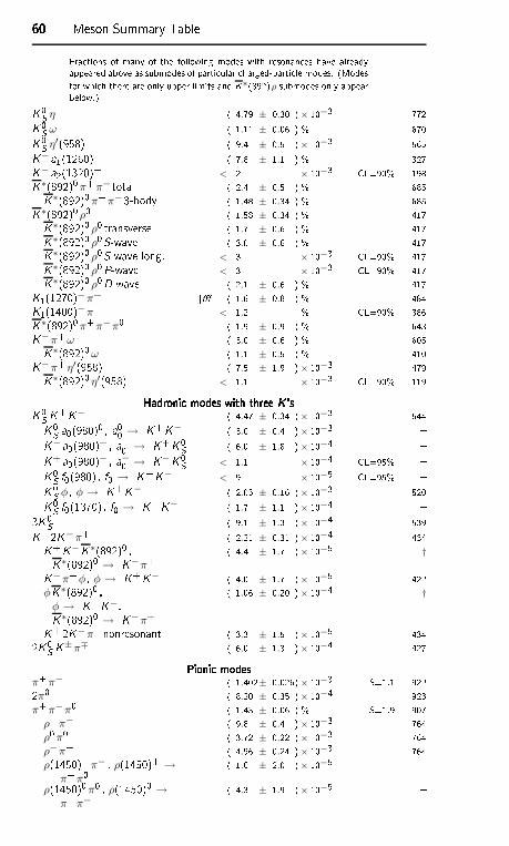
60606060 Meson Summary TableFra tions of many of the following modes with resonan es have alreadyappeared above as submodes of parti ular harged-parti le modes. (Modesfor whi h there are only upper limits and K∗(892)ρ submodes only appearbelow.)K0S η ( 4.79 ± 0.30 )× 10−3 772K0S ω ( 1.11 ± 0.06 ) % 670K0S η′(958) ( 9.4 ± 0.5 )× 10−3 565K− a1(1260)+ ( 7.8 ± 1.1 ) % 327K− a2(1320)+ < 2 × 10⁻³ CL=90% 198K∗(892)0π+π− total ( 2.4 ± 0.5 ) % 685K∗(892)0π+π−3-body ( 1.48 ± 0.34 ) % 685K∗(892)0 ρ0 ( 1.58 ± 0.34 ) % 417K∗(892)0 ρ0 transverse ( 1.7 ± 0.6 ) % 417K∗(892)0 ρ0S-wave ( 3.0 ± 0.6 ) % 417K∗(892)0 ρ0S-wave long. < 3 × 10⁻³ CL=90% 417K∗(892)0 ρ0P-wave < 3 × 10⁻³ CL=90% 417K∗(892)0 ρ0D-wave ( 2.1 ± 0.6 ) % 417K1(1270)−π+ [f ( 1.6 ± 0.8 ) % 484K1(1400)−π+ < 1.2 % CL=90% 386K∗(892)0π+π−π0 ( 1.9 ± 0.9 ) % 643K−π+ω ( 3.0 ± 0.6 ) % 605K∗(892)0ω ( 1.1 ± 0.5 ) % 410K−π+ η′(958) ( 7.5 ± 1.9 )× 10−3 479K∗(892)0 η′(958) < 1.1 × 10⁻³ CL=90% 119Hadroni modes with three K 'sHadroni modes with three K 'sHadroni modes with three K 'sHadroni modes with three K 'sK0S K+K− ( 4.47 ± 0.34 )× 10−3 544K0S a0(980)0 , a00 → K+K− ( 3.0 ± 0.4 )× 10−3 K− a0(980)+ , a+0 → K+K0S ( 6.0 ± 1.8 )× 10−4 K+ a0(980)− , a−0 → K−K0S < 1.1 × 10⁻⁴ CL=95% K0S f0(980), f0 → K+K− < 9 × 10⁻⁵ CL=95% K0S φ , φ → K+K− ( 2.05 ± 0.16 )× 10−3 520K0S f0(1370), f0 → K+K− ( 1.7 ± 1.1 )× 10−4 3K0S ( 9.1 ± 1.3 )× 10−4 539K+2K−π+ ( 2.21 ± 0.31 )× 10−4 434K+K−K∗(892)0 ,K∗(892)0 → K−π+ ( 4.4 ± 1.7 )× 10−5 †K−π+φ , φ → K+K− ( 4.0 ± 1.7 )× 10−5 422φK∗(892)0 ,
φ → K+K−,K∗(892)0 → K−π+ ( 1.06 ± 0.20 )× 10−4 †K+2K−π+nonresonant ( 3.3 ± 1.5 )× 10−5 4342K0S K±π∓ ( 6.0 ± 1.3 )× 10−4 427Pioni modesPioni modesPioni modesPioni modesπ+π− ( 1.402± 0.026)× 10−3 S=1.1 9222π0 ( 8.20 ± 0.35 )× 10−4 923π+π−π0 ( 1.43 ± 0.06 ) % S=1.9 907
ρ+π− ( 9.8 ± 0.4 )× 10−3 764ρ0π0 ( 3.72 ± 0.22 )× 10−3 764ρ−π+ ( 4.96 ± 0.24 )× 10−3 764ρ(1450)+π− , ρ(1450)+ →
π+π0 ( 1.6 ± 2.0 )× 10−5 ρ(1450)0π0 , ρ(1450)0 →
π+π−( 4.3 ± 1.9 )× 10−5
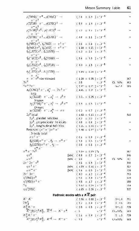
Meson Summary Table 61616161ρ(1450)−π+ , ρ(1450)− →
π−π0 ( 2.6 ± 0.4 )× 10−4 ρ(1700)+π− , ρ(1700)+ →
π+π0 ( 5.9 ± 1.4 )× 10−4 ρ(1700)0π0 , ρ(1700)0 →
π+π−( 7.2 ± 1.7 )× 10−4
ρ(1700)−π+ , ρ(1700)− →π−π0 ( 4.6 ± 1.1 )× 10−4 f0(980)π0 , f0(980) → π+π− ( 3.6 ± 0.8 )× 10−5 f0(500)π0 , f0(500) → π+π− ( 1.18 ± 0.21 )× 10−4 f0(1370)π0 , f0(1370) →π+π−
( 5.3 ± 2.1 )× 10−5 f0(1500)π0 , f0(1500) →π+π−
( 5.6 ± 1.5 )× 10−5 f0(1710)π0 , f0(1710) →π+π−
( 4.4 ± 1.5 )× 10−5 f2(1270)π0 , f2(1270) →π+π−
( 1.89 ± 0.20 )× 10−4 π+π−π0 nonresonant ( 1.20 ± 0.35 )× 10−4 9073π0 < 3.5 × 10⁻⁴ CL=90% 9082π+2π− ( 7.42 ± 0.21 )× 10−3 S=1.1 880a1(1260)+π− , a+1 → 2π+π−total ( 4.45 ± 0.31 )× 10−3 a1(1260)+π− , a+1 → ρ0π+S-wave ( 3.21 ± 0.25 )× 10−3 a1(1260)+π− , a+1 → ρ0π+D-wave ( 1.9 ± 0.5 )× 10−4 a1(1260)+π− , a+1 → σπ+ ( 6.2 ± 0.7 )× 10−4 2ρ0 total ( 1.82 ± 0.13 )× 10−3 5182ρ0 , parallel heli ities ( 8.2 ± 3.2 )× 10−5 2ρ0 , perpendi ular heli ities ( 4.8 ± 0.6 )× 10−4 2ρ0 , longitudinal heli ities ( 1.25 ± 0.10 )× 10−3 Resonant (π+π−)π+π−3-body total ( 1.48 ± 0.12 )× 10−3
σπ+π− ( 6.1 ± 0.9 )× 10−4 f0(980)π+π− , f0 → π+π− ( 1.8 ± 0.5 )× 10−4 f2(1270)π+π− , f2 →π+π−
( 3.6 ± 0.6 )× 10−4 π+π−2π0 ( 1.00 ± 0.09 ) % 882
ηπ0 [hhh ( 6.8 ± 0.7 )× 10−4 846ωπ0 [hhh < 2.6 × 10⁻⁴ CL=90% 7612π+2π−π0 ( 4.1 ± 0.5 )× 10−3 844ηπ+π− [hhh ( 1.09 ± 0.16 )× 10−3 827ωπ+π− [hhh ( 1.6 ± 0.5 )× 10−3 7383π+3π− ( 4.2 ± 1.2 )× 10−4 795
η′(958)π0 ( 9.0 ± 1.4 )× 10−4 678η′(958)π+π− ( 4.5 ± 1.7 )× 10−4 6502η ( 1.67 ± 0.20 )× 10−3 754ηη′(958) ( 1.05 ± 0.26 )× 10−3 537Hadroni modes with a K K pairHadroni modes with a K K pairHadroni modes with a K K pairHadroni modes with a K K pairK+K− ( 3.96 ± 0.08 )× 10−3 S=1.4 7912K0S ( 1.7 ± 0.4 )× 10−4 S=2.5 789K0S K−π+ ( 3.5 ± 0.5 )× 10−3 S=1.2 739K∗(892)0K0S , K∗0 → K−π+ < 5 × 10⁻⁴ CL=90% 608K0S K+π− ( 2.1 ± 0.4 )× 10−3 S=1.3 739K∗(892)0K0S , K∗0 → K+π− < 1.8 × 10⁻⁴ CL=90% 608
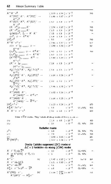
62626262 Meson Summary TableK+K−π0 ( 3.29 ± 0.14 )× 10−3 743K∗(892)+K−, K∗(892)+ →K+π0 ( 1.46 ± 0.07 )× 10−3 K∗(892)−K+, K∗(892)− →K−π0 ( 5.2 ± 0.4 )× 10−4 (K+π0)S−waveK− ( 2.34 ± 0.17 )× 10−3 743(K−π0)S−waveK+ ( 1.3 ± 0.4 )× 10−4 743f0(980)π0, f0 → K+K− ( 3.5 ± 0.6 )× 10−4 φπ0, φ → K+K− ( 6.4 ± 0.4 )× 10−4 2K0S π0 < 5.9 × 10⁻⁴ 740K+K−π+π− ( 2.43 ± 0.12 )× 10−3 677φ(π+π−)S−wave, φ →K+K−
( 2.50 ± 0.33 )× 10−4 614(φρ0)S−wave, φ → K+K− ( 9.3 ± 1.2 )× 10−4 250(φρ0)D−wave, φ → K+K− ( 8.3 ± 2.3 )× 10−5 (K∗0K∗0)S−wave, K∗0 →K±π∓( 1.48 ± 0.30 )× 10−4 (K−π+)P−wave,(K+π−)S−wave, ( 2.6 ± 0.5 )× 10−4 K1(1270)+K−, K1(1270)+ →K∗0π+ ( 1.8 ± 0.5 )× 10−4 K1(1270)+K−, K1(1270)+ →
ρ0K+ ( 1.14 ± 0.26 )× 10−4 K1(1270)−K+, K1(1270)− →K∗0π−( 2.2 ± 1.2 )× 10−5 K1(1270)−K+, K1(1270)− →
ρ0K−( 1.46 ± 0.25 )× 10−4 K∗(1410)+K−,K∗(1410)+ → K∗0π+ ( 1.02 ± 0.26 )× 10−4 K∗(1410)−K+,K∗(1410)− → K∗0π−( 1.14 ± 0.25 )× 10−4 2K0S π+π− ( 1.23 ± 0.24 )× 10−3 673K0S K−2π+π− < 1.5 × 10⁻⁴ CL=90% 595K+K−π+π−π0 ( 3.1 ± 2.0 )× 10−3 600Other K K X modes. They in lude all de ay modes of the φ, η, and ω.
φη ( 1.4 ± 0.5 )× 10−4 489φω < 2.1 × 10⁻³ CL=90% 238Radiative modesRadiative modesRadiative modesRadiative modesρ0 γ < 2.4 × 10⁻⁴ CL=90% 771ωγ < 2.4 × 10⁻⁴ CL=90% 768φγ ( 2.70 ± 0.35 )× 10−5 654K∗(892)0 γ ( 3.27 ± 0.34 )× 10−4 719Doubly Cabibbo suppressed (DC ) modes orDoubly Cabibbo suppressed (DC ) modes orDoubly Cabibbo suppressed (DC ) modes orDoubly Cabibbo suppressed (DC ) modes orC = 2 forbidden via mixing (C2M) modesC = 2 forbidden via mixing (C2M) modesC = 2 forbidden via mixing (C2M) modesC = 2 forbidden via mixing (C2M) modesK+ ℓ−νℓ via D0 < 2.2 × 10⁻⁵ CL=90% K+or K∗(892)+ e−νe viaD0 < 6 × 10⁻⁵ CL=90% K+π− DC ( 1.47 ± 0.07 )× 10−4 S=2.8 861K+π− via DCS ( 1.31 ± 0.08 )× 10−4 K+π− via D0 < 1.6 × 10⁻⁵ CL=95% 861K0S π+π− in D0 → D0 < 1.8 × 10⁻⁴ CL=95% K∗(892)+π− ,K∗(892)+ → K0S π+ DC ( 1.14 + 0.60
− 0.34 )× 10−4 711
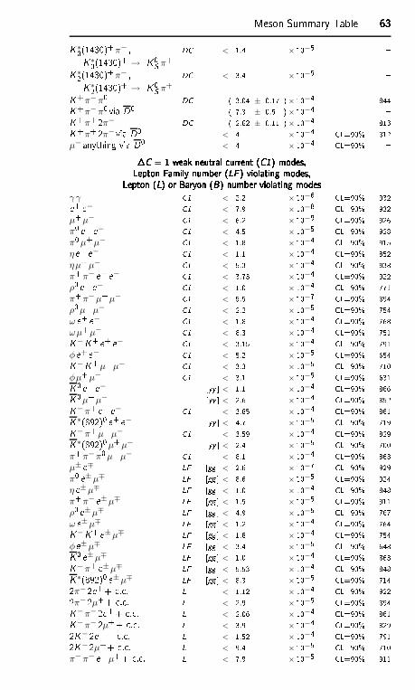
Meson Summary Table 63636363K∗0(1430)+π− ,K∗0(1430)+ → K0S π+ DC < 1.4 × 10−5 K∗2(1430)+π− ,K∗2(1430)+ → K0S π+ DC < 3.4 × 10⁻⁵ K+π−π0 DC ( 3.04 ± 0.17 )× 10−4 844K+π−π0 via D0 ( 7.3 ± 0.5 )× 10−4 K+π+ 2π− DC ( 2.62 ± 0.11 )× 10−4 813K+π+ 2π− via D0 < 4 × 10⁻⁴ CL=90% 812µ− anything via D0 < 4 × 10⁻⁴ CL=90% C = 1 weak neutral urrent (C1) modes,C = 1 weak neutral urrent (C1) modes,C = 1 weak neutral urrent (C1) modes,C = 1 weak neutral urrent (C1) modes,Lepton Family number (LF ) violating modes,Lepton Family number (LF ) violating modes,Lepton Family number (LF ) violating modes,Lepton Family number (LF ) violating modes,Lepton (L) or Baryon (B) number violating modesLepton (L) or Baryon (B) number violating modesLepton (L) or Baryon (B) number violating modesLepton (L) or Baryon (B) number violating modesγ γ C1 < 2.2 × 10⁻⁶ CL=90% 932e+ e− C1 < 7.9 × 10⁻⁸ CL=90% 932µ+µ− C1 < 6.2 × 10⁻⁹ CL=90% 926π0 e+ e− C1 < 4.5 × 10⁻⁵ CL=90% 928π0µ+µ− C1 < 1.8 × 10⁻⁴ CL=90% 915ηe+ e− C1 < 1.1 × 10⁻⁴ CL=90% 852ηµ+µ− C1 < 5.3 × 10⁻⁴ CL=90% 838π+π− e+ e− C1 < 3.73 × 10⁻⁴ CL=90% 922ρ0 e+ e− C1 < 1.0 × 10⁻⁴ CL=90% 771π+π−µ+µ− C1 < 5.5 × 10⁻⁷ CL=90% 894ρ0µ+µ− C1 < 2.2 × 10⁻⁵ CL=90% 754ω e+ e− C1 < 1.8 × 10⁻⁴ CL=90% 768ωµ+µ− C1 < 8.3 × 10⁻⁴ CL=90% 751K−K+ e+ e− C1 < 3.15 × 10⁻⁴ CL=90% 791φe+ e− C1 < 5.2 × 10⁻⁵ CL=90% 654K−K+µ+µ− C1 < 3.3 × 10⁻⁵ CL=90% 710φµ+µ− C1 < 3.1 × 10⁻⁵ CL=90% 631K0 e+ e− [yy < 1.1 × 10⁻⁴ CL=90% 866K0µ+µ− [yy < 2.6 × 10⁻⁴ CL=90% 852K−π+ e+ e− C1 < 3.85 × 10⁻⁴ CL=90% 861K∗(892)0 e+ e− [yy < 4.7 × 10⁻⁵ CL=90% 719K−π+µ+µ− C1 < 3.59 × 10⁻⁴ CL=90% 829K∗(892)0µ+µ− [yy < 2.4 × 10⁻⁵ CL=90% 700π+π−π0µ+µ− C1 < 8.1 × 10⁻⁴ CL=90% 863µ± e∓ LF [gg < 2.6 × 10⁻⁷ CL=90% 929π0 e±µ∓ LF [gg < 8.6 × 10⁻⁵ CL=90% 924ηe±µ∓ LF [gg < 1.0 × 10⁻⁴ CL=90% 848π+π− e±µ∓ LF [gg < 1.5 × 10⁻⁵ CL=90% 911ρ0 e±µ∓ LF [gg < 4.9 × 10⁻⁵ CL=90% 767ω e±µ∓ LF [gg < 1.2 × 10⁻⁴ CL=90% 764K−K+ e±µ∓ LF [gg < 1.8 × 10⁻⁴ CL=90% 754φe±µ∓ LF [gg < 3.4 × 10⁻⁵ CL=90% 648K0 e±µ∓ LF [gg < 1.0 × 10⁻⁴ CL=90% 863K−π+ e±µ∓ LF [gg < 5.53 × 10⁻⁴ CL=90% 848K∗(892)0 e±µ∓ LF [gg < 8.3 × 10⁻⁵ CL=90% 7142π−2e++ . . L < 1.12 × 10⁻⁴ CL=90% 9222π−2µ++ . . L < 2.9 × 10⁻⁵ CL=90% 894K−π− 2e++ . . L < 2.06 × 10⁻⁴ CL=90% 861K−π− 2µ++ . . L < 3.9 × 10⁻⁴ CL=90% 8292K−2e++ . . L < 1.52 × 10⁻⁴ CL=90% 7912K−2µ++ . . L < 9.4 × 10⁻⁵ CL=90% 710π−π− e+µ++ . . L < 7.9 × 10⁻⁵ CL=90% 911
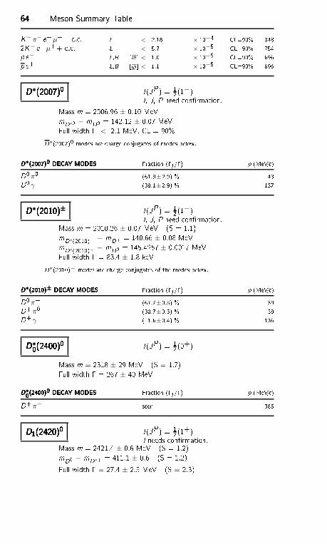
64646464 Meson Summary TableK−π− e+µ++ . . L < 2.18 × 10⁻⁴ CL=90% 8482K− e+µ++ . . L < 5.7 × 10⁻⁵ CL=90% 754p e− L,B [iii < 1.0 × 10⁻⁵ CL=90% 696p e+ L,B [jjj < 1.1 × 10⁻⁵ CL=90% 696D∗(2007)0D∗(2007)0D∗(2007)0D∗(2007)0 I (JP ) = 12 (1−)I, J, P need onrmation.Mass m = 2006.96 ± 0.10 MeVmD∗0 − mD0 = 142.12 ± 0.07 MeVFull width < 2.1 MeV, CL = 90%D∗(2007)0 modes are harge onjugates of modes below.D∗(2007)0 DECAY MODESD∗(2007)0 DECAY MODESD∗(2007)0 DECAY MODESD∗(2007)0 DECAY MODES Fra tion (i /) p (MeV/ )D0π0 (61.9±2.9) % 43D0 γ (38.1±2.9) % 137D∗(2010)±D∗(2010)±D∗(2010)±D∗(2010)± I (JP ) = 12 (1−)I, J, P need onrmation.Mass m = 2010.26 ± 0.07 MeV (S = 1.1)mD∗(2010)+ − mD+ = 140.66 ± 0.08 MeVmD∗(2010)+ − mD0 = 145.4257 ± 0.0017 MeVFull width = 83.4 ± 1.8 keVD∗(2010)− modes are harge onjugates of the modes below.D∗(2010)± DECAY MODESD∗(2010)± DECAY MODESD∗(2010)± DECAY MODESD∗(2010)± DECAY MODES Fra tion (i /) p (MeV/ )D0π+ (67.7±0.5) % 39D+π0 (30.7±0.5) % 38D+ γ ( 1.6±0.4) % 136D∗0(2400)0D∗0(2400)0D∗0(2400)0D∗0(2400)0 I (JP ) = 12 (0+)Mass m = 2318 ± 29 MeV (S = 1.7)Full width = 267 ± 40 MeVD∗0(2400)0 DECAY MODESD∗0(2400)0 DECAY MODESD∗0(2400)0 DECAY MODESD∗0(2400)0 DECAY MODES Fra tion (i /) p (MeV/ )D+π− seen 385D1(2420)0D1(2420)0D1(2420)0D1(2420)0 I (JP ) = 12 (1+)I needs onrmation.Mass m = 2421.4 ± 0.6 MeV (S = 1.2)mD01 − mD∗+ = 411.1 ± 0.6 (S = 1.2)Full width = 27.4 ± 2.5 MeV (S = 2.3)
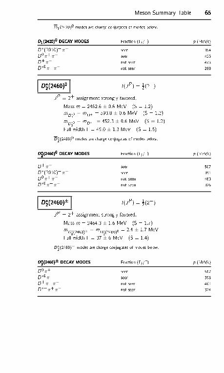
Meson Summary Table 65656565D1(2420)0 modes are harge onjugates of modes below.D1(2420)0 DECAY MODESD1(2420)0 DECAY MODESD1(2420)0 DECAY MODESD1(2420)0 DECAY MODES Fra tion (i /) p (MeV/ )D∗(2010)+π− seen 354D0π+π− seen 425D+π− not seen 473D∗0π+π− not seen 280D∗2(2460)0D∗2(2460)0D∗2(2460)0D∗2(2460)0 I (JP ) = 12 (2+)JP = 2+ assignment strongly favored.Mass m = 2462.6 ± 0.6 MeV (S = 1.2)mD∗02 − mD+ = 593.0 ± 0.6 MeV (S = 1.2)mD∗02 − mD∗+ = 452.3 ± 0.6 MeV (S = 1.2)Full width = 49.0 ± 1.3 MeV (S = 1.5)D∗2(2460)0 modes are harge onjugates of modes below.D∗2(2460)0 DECAY MODESD∗2(2460)0 DECAY MODESD∗2(2460)0 DECAY MODESD∗2(2460)0 DECAY MODES Fra tion (i /) p (MeV/ )D+π− seen 507D∗(2010)+π− seen 391D0π+π− not seen 463D∗0π+π− not seen 326D∗2(2460)±D∗2(2460)±D∗2(2460)±D∗2(2460)± I (JP ) = 12 (2+)JP = 2+ assignment strongly favored.Mass m = 2464.3 ± 1.6 MeV (S = 1.7)mD∗2(2460)± − mD∗2(2460)0 = 2.4 ± 1.7 MeVFull width = 37 ± 6 MeV (S = 1.4)D∗2(2460)− modes are harge onjugates of modes below.D∗2(2460)± DECAY MODESD∗2(2460)± DECAY MODESD∗2(2460)± DECAY MODESD∗2(2460)± DECAY MODES Fra tion (i /) p (MeV/ )D0π+ seen 512D∗0π+ seen 395D+π+π− not seen 461D∗+π+π− not seen 324
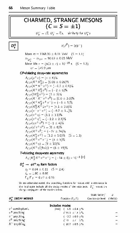
66666666 Meson Summary TableCHARMED, STRANGE MESONSCHARMED, STRANGE MESONSCHARMED, STRANGE MESONSCHARMED, STRANGE MESONS(C = S = ±1)(C = S = ±1)(C = S = ±1)(C = S = ±1)D+s = s , D−s = s, similarly for D∗s 'sD±sD±sD±sD±s I (JP ) = 0(0−)Mass m = 1968.30 ± 0.11 MeV (S = 1.1)mD±s − mD± = 98.69 ± 0.05 MeVMean life τ = (500 ± 7)× 10−15 s (S = 1.3) τ = 149.9 µmCP-violating de ay-rate asymmetriesCP-violating de ay-rate asymmetriesCP-violating de ay-rate asymmetriesCP-violating de ay-rate asymmetriesACP (µ±ν) = (5 ± 6)%ACP (K±K0S ) = (0.08 ± 0.26)%ACP (K+K−π±) = (−0.5 ± 0.9)%ACP (K±K0S π0) = (−2 ± 6)%ACP (2K0S π±) = (3 ± 5)%ACP (K+K−π±π0) = (0.0 ± 3.0)%ACP (K±K0S π+π−) = (−6 ± 5)%ACP (K0S K∓2π±) = (4.1 ± 2.8)%ACP (π+π−π±) = (−0.7 ± 3.1)%ACP (π± η) = (1.1 ± 3.1)%ACP (π± η′) = (−2.2 ± 2.3)%ACP (ηπ±π0) = (−1 ± 4)%ACP (η′π±π0) = (0 ± 8)%ACP (K±π0) = (−27 ± 24)%ACP (K0S π±) = (1.2 ± 1.0)% (S = 1.3)ACP (K±π+π−) = (4 ± 5)%ACP (K±η) = (9 ± 15)%ACP (K±η′(958)) = (6 ± 19)%T-violating de ay-rate asymmetryT-violating de ay-rate asymmetryT-violating de ay-rate asymmetryT-violating de ay-rate asymmetryAT (K0S K±π+π−) = (−14 ± 8)× 10−3 [rr D+s → φℓ+ νℓ form fa torsD+s → φℓ+ νℓ form fa torsD+s → φℓ+ νℓ form fa torsD+s → φℓ+ νℓ form fa torsr2 = 0.84 ± 0.11 (S = 2.4)rv = 1.80 ± 0.08L/T = 0.72 ± 0.18Unless otherwise noted, the bran hing fra tions for modes with a resonan e inthe nal state in lude all the de ay modes of the resonan e. D−s modes are harge onjugates of the modes below. S ale fa tor/ pD+s DECAY MODESD+s DECAY MODESD+s DECAY MODESD+s DECAY MODES Fra tion (i /) Conden e level (MeV/ )In lusive modesIn lusive modesIn lusive modesIn lusive modese+ semileptoni [kkk ( 6.5 ±0.4 ) % π+ anything (119.3 ±1.4 ) % π− anything ( 43.2 ±0.9 ) % π0 anything (123 ±7 ) % K− anything ( 18.7 ±0.5 ) %
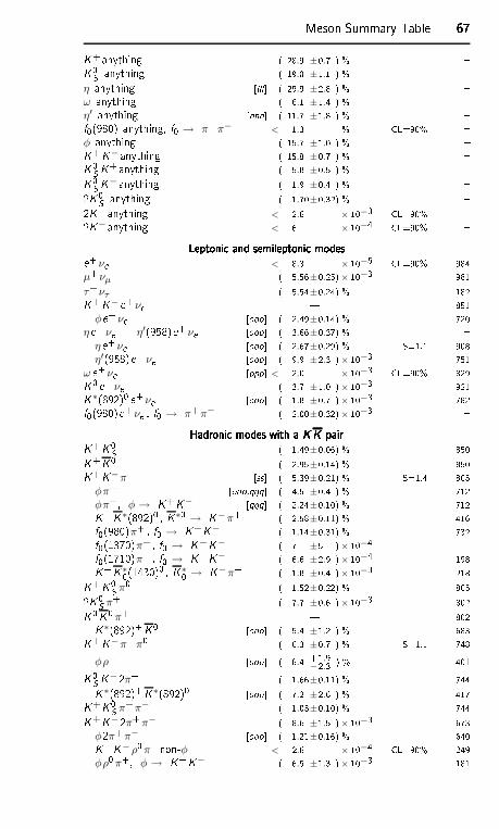
Meson Summary Table 67676767K+ anything ( 28.9 ±0.7 ) % K0S anything ( 19.0 ±1.1 ) % η anything [lll ( 29.9 ±2.8 ) % ω anything ( 6.1 ±1.4 ) % η′ anything [nnn ( 11.7 ±1.8 ) % f0(980) anything, f0 → π+π− < 1.3 % CL=90% φ anything ( 15.7 ±1.0 ) % K+K− anything ( 15.8 ±0.7 ) % K0S K+ anything ( 5.8 ±0.5 ) % K0S K− anything ( 1.9 ±0.4 ) % 2K0S anything ( 1.70±0.32) % 2K+ anything < 2.6 × 10⁻³ CL=90% 2K− anything < 6 × 10⁻⁴ CL=90% Leptoni and semileptoni modesLeptoni and semileptoni modesLeptoni and semileptoni modesLeptoni and semileptoni modese+ νe < 8.3 × 10⁻⁵ CL=90% 984µ+νµ ( 5.56±0.25)× 10−3 981τ+ ντ ( 5.54±0.24) % 182K+K− e+νe | 851
φe+ νe [ooo ( 2.49±0.14) % 720ηe+ νe + η′(958)e+ νe [ooo ( 3.66±0.37) %
ηe+ νe [ooo ( 2.67±0.29) % S=1.1 908η′(958)e+ νe [ooo ( 9.9 ±2.3 )× 10−3 751
ω e+ νe [ppp < 2.0 × 10⁻³ CL=90% 829K0 e+ νe ( 3.7 ±1.0 )× 10−3 921K∗(892)0 e+νe [ooo ( 1.8 ±0.7 )× 10−3 782f0(980)e+ νe , f0 → π+π− ( 2.00±0.32)× 10−3 Hadroni modes with a K K pairHadroni modes with a K K pairHadroni modes with a K K pairHadroni modes with a K K pairK+K0S ( 1.49±0.06) % 850K+K0 ( 2.95±0.14) % 850K+K−π+ [ss ( 5.39±0.21) % S=1.4 805φπ+ [ooo,qqq ( 4.5 ±0.4 ) % 712φπ+, φ → K+K− [qqq ( 2.24±0.10) % 712K+K∗(892)0 , K∗0 → K−π+ ( 2.58±0.11) % 416f0(980)π+ , f0 → K+K− ( 1.14±0.31) % 732f0(1370)π+ , f0 → K+K− ( 7 ±5 )× 10−4 f0(1710)π+ , f0 → K+K− ( 6.6 ±2.9 )× 10−4 198K+K∗0(1430)0 , K∗0 → K−π+ ( 1.8 ±0.4 )× 10−3 218K+K0S π0 ( 1.52±0.22) % 8052K0S π+ ( 7.7 ±0.6 )× 10−3 802K0K0π+ | 802K∗(892)+K0 [ooo ( 5.4 ±1.2 ) % 683K+K−π+π0 ( 6.3 ±0.7 ) % S=1.1 748φρ+ [ooo ( 8.4 +1.9
−2.3 ) % 401K0S K−2π+ ( 1.66±0.11) % 744K∗(892)+K∗(892)0 [ooo ( 7.2 ±2.6 ) % 417K+K0S π+π− ( 1.03±0.10) % 744K+K−2π+π− ( 8.6 ±1.5 )× 10−3 673φ2π+π− [ooo ( 1.21±0.16) % 640K+K−ρ0π+non-φ < 2.6 × 10⁻⁴ CL=90% 249φρ0π+, φ → K+K− ( 6.5 ±1.3 )× 10−3 181
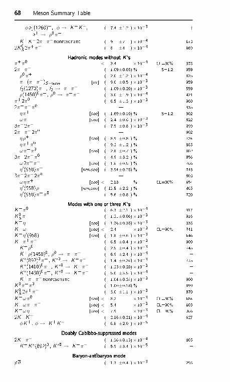
68686868 Meson Summary Tableφa1(1260)+, φ → K+K−,a+1 → ρ0π+ ( 7.4 ±1.2 )× 10−3 †K+K−2π+π− nonresonant ( 9 ±7 )× 10−4 6732K0S 2π+π− ( 8 ±4 )× 10−4 669Hadroni modes without K 'sHadroni modes without K 'sHadroni modes without K 'sHadroni modes without K 's
π+π0 < 3.4 × 10⁻⁴ CL=90% 9752π+π− ( 1.09±0.05) % S=1.2 959ρ0π+ ( 2.0 ±1.2 )× 10−4 825π+ (π+π−)S−wave [rrr ( 9.0 ±0.5 )× 10−3 959f2(1270)π+ , f2 → π+π− ( 1.09±0.20)× 10−3 559ρ(1450)0π+ , ρ0 → π+π− ( 3.0 ±1.9 )× 10−4 421
π+ 2π0 ( 6.5 ±1.3 )× 10−3 9602π+π−π0 | 935ηπ+ [ooo ( 1.69±0.10) % S=1.2 902ωπ+ [ooo ( 2.4 ±0.6 )× 10−3 8223π+2π− ( 7.9 ±0.8 )× 10−3 8992π+π− 2π0 | 902ηρ+ [ooo ( 8.9 ±0.8 ) % 724ηπ+π0 ( 9.2 ±1.2 ) % 885ωπ+π0 [ooo ( 2.8 ±0.7 ) % 8023π+2π−π0 ( 4.9 ±3.2 ) % 856ω2π+π− [ooo ( 1.6 ±0.5 ) % 766η′(958)π+ [nnn,ooo ( 3.94±0.25) % 7433π+2π−2π0 | 803ωηπ+ [ooo < 2.13 % CL=90% 654η′(958)ρ+ [nnn,ooo ( 12.5 ±2.2 ) % 465η′(958)π+π0 ( 5.6 ±0.8 ) % 720Modes with one or three K 'sModes with one or three K 'sModes with one or three K 'sModes with one or three K 'sK+π0 ( 6.3 ±2.1 )× 10−4 917K0S π+ ( 1.21±0.06)× 10−3 916K+η [ooo ( 1.76±0.35)× 10−3 835K+ω [ooo < 2.4 × 10⁻³ CL=90% 741K+η′(958) [ooo ( 1.8 ±0.6 )× 10−3 646K+π+π− ( 6.5 ±0.4 )× 10−3 900K+ρ0 ( 2.5 ±0.4 )× 10−3 745K+ρ(1450)0 , ρ0 → π+π− ( 6.9 ±2.4 )× 10−4 K∗(892)0π+ , K∗0 → K+π− ( 1.41±0.24)× 10−3 775K∗(1410)0π+ , K∗0 → K+π− ( 1.23±0.28)× 10−3 K∗(1430)0π+ , K∗0 → K+π− ( 5.0 ±3.5 )× 10−4 K+π+π−nonresonant ( 1.04±0.34)× 10−3 900K0π+π0 ( 1.00±0.18) % 899K0S 2π+π− ( 3.0 ±1.1 )× 10−3 870K+ωπ0 [ooo < 8.2 × 10⁻³ CL=90% 684K+ωπ+π− [ooo < 5.4 × 10⁻³ CL=90% 603K+ωη [ooo < 7.9 × 10⁻³ CL=90% 3662K+K− ( 2.16±0.21)× 10−4 627φK+ , φ → K+K− ( 8.8 ±2.0 )× 10−5 Doubly Cabibbo-suppressed modesDoubly Cabibbo-suppressed modesDoubly Cabibbo-suppressed modesDoubly Cabibbo-suppressed modes2K+π− ( 1.26±0.13)× 10−4 805K+K∗(892)0 , K∗0 → K+π− ( 5.9 ±3.4 )× 10−5 Baryon-antibaryon modeBaryon-antibaryon modeBaryon-antibaryon modeBaryon-antibaryon modepn ( 1.3 ±0.4 )× 10−3 295
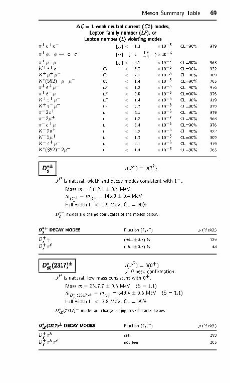
Meson Summary Table 69696969C = 1 weak neutral urrent (C1) modes,C = 1 weak neutral urrent (C1) modes,C = 1 weak neutral urrent (C1) modes,C = 1 weak neutral urrent (C1) modes,Lepton family number (LF), orLepton family number (LF), orLepton family number (LF), orLepton family number (LF), orLepton number (L) violating modesLepton number (L) violating modesLepton number (L) violating modesLepton number (L) violating modesπ+ e+ e− [yy < 1.3 × 10⁻⁵ CL=90% 979π+φ, φ → e+ e− [xx ( 6 +8
−4 )× 10−6 π+µ+µ− [yy < 4.1 × 10⁻⁷ CL=90% 968K+ e+ e− C1 < 3.7 × 10⁻⁶ CL=90% 922K+µ+µ− C1 < 2.1 × 10⁻⁵ CL=90% 909K∗(892)+µ+µ− C1 < 1.4 × 10⁻³ CL=90% 765π+ e+µ− LF < 1.2 × 10⁻⁵ CL=90% 976π+ e−µ+ LF < 2.0 × 10⁻⁵ CL=90% 976K+ e+µ− LF < 1.4 × 10⁻⁵ CL=90% 919K+ e−µ+ LF < 9.7 × 10⁻⁶ CL=90% 919π− 2e+ L < 4.1 × 10⁻⁶ CL=90% 979π− 2µ+ L < 1.2 × 10⁻⁷ CL=90% 968π− e+µ+ L < 8.4 × 10⁻⁶ CL=90% 976K−2e+ L < 5.2 × 10⁻⁶ CL=90% 922K−2µ+ L < 1.3 × 10⁻⁵ CL=90% 909K− e+µ+ L < 6.1 × 10⁻⁶ CL=90% 919K∗(892)− 2µ+ L < 1.4 × 10⁻³ CL=90% 765D∗±sD∗±sD∗±sD∗±s I (JP ) = 0(??)JP is natural, width and de ay modes onsistent with 1− .Mass m = 2112.1 ± 0.4 MeVmD∗±s − mD±s = 143.8 ± 0.4 MeVFull width < 1.9 MeV, CL = 90%D∗−s modes are harge onjugates of the modes below.D∗+s DECAY MODESD∗+s DECAY MODESD∗+s DECAY MODESD∗+s DECAY MODES Fra tion (i /) p (MeV/ )D+s γ (94.2±0.7) % 139D+s π0 ( 5.8±0.7) % 48D∗s0(2317)±D∗s0(2317)±D∗s0(2317)±D∗s0(2317)± I (JP ) = 0(0+)J, P need onrmation.JP is natural, low mass onsistent with 0+.Mass m = 2317.7 ± 0.6 MeV (S = 1.1)mD∗s0(2317)± − mD±s = 349.4 ± 0.6 MeV (S = 1.1)Full width < 3.8 MeV, CL = 95%D∗s0(2317)− modes are harge onjugates of modes below.D∗s0(2317)± DECAY MODESD∗s0(2317)± DECAY MODESD∗s0(2317)± DECAY MODESD∗s0(2317)± DECAY MODES Fra tion (i /) p (MeV/ )D+s π0 seen 298D+s π0π0 not seen 205
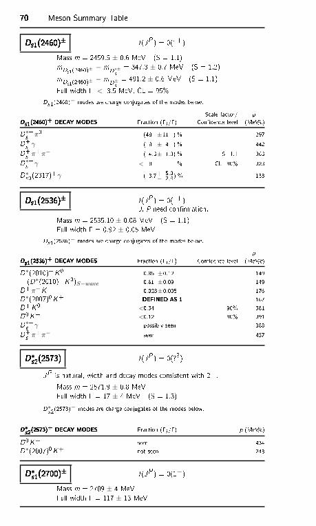
70707070 Meson Summary TableDs1(2460)±Ds1(2460)±Ds1(2460)±Ds1(2460)± I (JP ) = 0(1+)Mass m = 2459.5 ± 0.6 MeV (S = 1.1)mDs1(2460)± − mD∗±s = 347.3 ± 0.7 MeV (S = 1.2)mDs1(2460)± − mD±s = 491.2 ± 0.6 MeV (S = 1.1)Full width < 3.5 MeV, CL = 95%Ds1(2460)− modes are harge onjugates of the modes below. S ale fa tor/ pDs1(2460)+ DECAY MODESDs1(2460)+ DECAY MODESDs1(2460)+ DECAY MODESDs1(2460)+ DECAY MODES Fra tion (i /) Conden e level (MeV/ )D∗+s π0 (48 ±11 ) % 297D+s γ (18 ± 4 ) % 442D+s π+π− ( 4.3± 1.3) % S=1.1 363D∗+s γ < 8 % CL=90% 323D∗s0(2317)+ γ ( 3.7+ 5.0− 2.4) % 138Ds1(2536)±Ds1(2536)±Ds1(2536)±Ds1(2536)± I (JP ) = 0(1+)J, P need onrmation.Mass m = 2535.10 ± 0.08 MeV (S = 1.1)Full width = 0.92 ± 0.05 MeVDs1(2536)− modes are harge onjugates of the modes below. pDs1(2536)+ DECAY MODESDs1(2536)+ DECAY MODESDs1(2536)+ DECAY MODESDs1(2536)+ DECAY MODES Fra tion (i /) Conden e level (MeV/ )D∗(2010)+K0 0.85 ±0.12 149(D∗(2010)+K0)S−wave 0.61 ±0.09 149D+π−K+ 0.028±0.005 176D∗(2007)0K+ DEFINED AS 1DEFINED AS 1DEFINED AS 1DEFINED AS 1 167D+K0 <0.34 90% 381D0K+ <0.12 90% 391D∗+s γ possibly seen 388D+s π+π− seen 437D∗s2(2573)D∗s2(2573)D∗s2(2573)D∗s2(2573) I (JP ) = 0(??)JP is natural, width and de ay modes onsistent with 2+ .Mass m = 2571.9 ± 0.8 MeVFull width = 17 ± 4 MeV (S = 1.3)D∗s2(2573)− modes are harge onjugates of the modes below.D∗s2(2573)+ DECAY MODESD∗s2(2573)+ DECAY MODESD∗s2(2573)+ DECAY MODESD∗s2(2573)+ DECAY MODES Fra tion (i /) p (MeV/ )D0K+ seen 434D∗(2007)0K+ not seen 243D∗s1(2700)±D∗s1(2700)±D∗s1(2700)±D∗s1(2700)± I (JP ) = 0(1−)Mass m = 2709 ± 4 MeVFull width = 117 ± 13 MeV
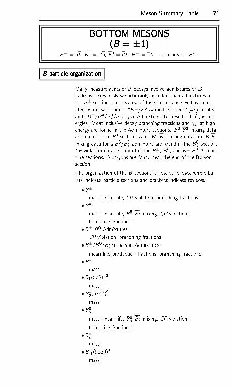
Meson Summary Table 71717171BOTTOM MESONSBOTTOM MESONSBOTTOM MESONSBOTTOM MESONS(B = ±1)(B = ±1)(B = ±1)(B = ±1)B+ = ub, B0 = db, B0 = d b, B− = ub, similarly for B∗'sB-parti le organizationB-parti le organizationB-parti le organizationB-parti le organizationMany measurements of B de ays involve admixtures of Bhadrons. Previously we arbitrarily in luded su h admixtures inthe B± se tion, but be ause of their importan e we have re-ated two new se tions: \B±/B0 Admixture" for (4S) resultsand \B±/B0/B0s /b-baryon Admixture" for results at higher en-ergies. Most in lusive de ay bran hing fra tions and χb at highenergy are found in the Admixture se tions. B0-B0 mixing dataare found in the B0 se tion, while B0s -B0s mixing data and B-Bmixing data for a B0/B0s admixture are found in the B0s se tion.CP-violation data are found in the B±, B0, and B± B0 Admix-ture se tions. b-baryons are found near the end of the Baryonse tion.The organization of the B se tions is now as follows, where bul-lets indi ate parti le se tions and bra kets indi ate reviews.•B±mass, mean life, CP violation, bran hing fra tions•B0mass, mean life, B0-B0 mixing, CP violation,bran hing fra tions•B± B0 AdmixturesCP violation, bran hing fra tions•B±/B0/B0s /b-baryon Admixturesmean life, produ tion fra tions, bran hing fra tions•B∗mass•B1(5721)0mass•B∗2(5747)0mass•B0smass, mean life, B0s -B0s mixing, CP violation,bran hing fra tions•B∗smass•Bs1(5830)0mass
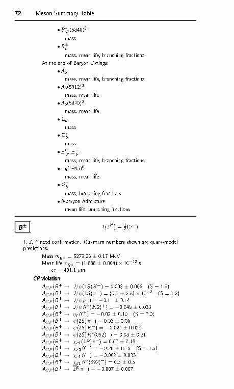
72727272 Meson Summary Table•B∗s2(5840)0mass•B± mass, mean life, bran hing fra tionsAt the end of Baryon Listings:• bmass, mean life, bran hing fra tions• b(5912)0mass, mean life• b(5920)0mass, mean life•bmass•∗bmass• 0b , −bmass, mean life, bran hing fra tions•b(5945)0mass, mean life•−bmass, bran hing fra tions• b-baryon Admixturemean life, bran hing fra tionsB±B±B±B± I (JP ) = 12 (0−)I , J , P need onrmation. Quantum numbers shown are quark-modelpredi tions.Mass mB± = 5279.26 ± 0.17 MeVMean life τB± = (1.638 ± 0.004)× 10−12 s τ = 491.1 µmCP violationCP violationCP violationCP violationACP (B+ → J/ψ(1S)K+) = 0.003 ± 0.006 (S = 1.8)ACP (B+ → J/ψ(1S)π+) = (0.1 ± 2.8)× 10−2 (S = 1.2)ACP (B+ → J/ψρ+) = −0.11 ± 0.14ACP (B+ → J/ψK∗(892)+) = −0.048 ± 0.033ACP (B+ → η K+) = −0.02 ± 0.10 (S = 2.0)ACP (B+ → ψ(2S)π+) = 0.03 ± 0.06ACP (B+ → ψ(2S)K+) = −0.024 ± 0.023ACP (B+ → ψ(2S)K∗(892)+) = 0.08 ± 0.21ACP (B+ → χ 1(1P)π+) = 0.07 ± 0.18ACP (B+ → χ 0K+) = −0.20 ± 0.18 (S = 1.5)ACP (B+ → χ 1K+) = −0.009 ± 0.033ACP (B+ → χ 1K∗(892)+) = 0.5 ± 0.5ACP (B+ → D0π+) = −0.007 ± 0.007
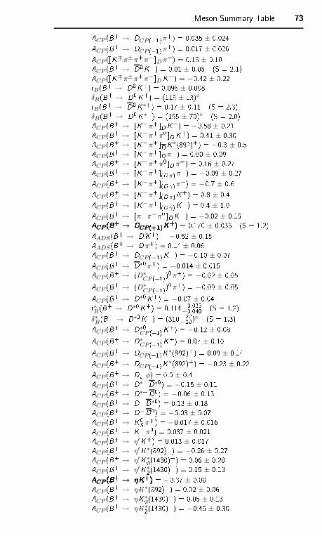
Meson Summary Table 73737373ACP (B+ → DCP (+1)π+) = 0.035 ± 0.024ACP (B+ → DCP (−1)π+) = 0.017 ± 0.026ACP ([K∓π±π+π− D π+) = 0.13 ± 0.10ACP (B+ → D0K+) = 0.01 ± 0.05 (S = 2.1)ACP ([K∓π±π+π− DK+) = −0.42 ± 0.22rB(B+ → D0K+) = 0.096 ± 0.008δB(B+ → D0K+) = (115 ± 13)rB(B+ → D0K∗+) = 0.17 ± 0.11 (S = 2.3)δB(B+ → D0K∗+) = (155 ± 70) (S = 2.0)ACP (B+ → [K−π+ DK+) = −0.58 ± 0.21ACP (B+ → [K−π+π0 DK+) = 0.41 ± 0.30ACP (B+ → [K−π+ DK∗(892)+) = −0.3 ± 0.5ACP (B+ → [K−π+ D π+) = 0.00 ± 0.09ACP (B+ → [K−π+π0 D π+) = 0.16 ± 0.27ACP (B+ → [K−π+ (D π)π+) = −0.09 ± 0.27ACP (B+ → [K−π+ (D γ)π+) = −0.7 ± 0.6ACP (B+ → [K−π+ (D π)K+) = 0.8 ± 0.4ACP (B+ → [K−π+ (D γ)K+) = 0.4 ± 1.0ACP (B+ → [π+π−π0 DK+) = −0.02 ± 0.15ACP (B+ → DCP (+1)K+)ACP (B+ → DCP (+1)K+)ACP (B+ → DCP (+1)K+)ACP (B+ → DCP (+1)K+) = 0.170 ± 0.033 (S = 1.2)AADS(B+ → DK+) = −0.52 ± 0.15AADS(B+ → D π+) = 0.14 ± 0.06ACP (B+ → DCP (−1)K+) = −0.10 ± 0.07ACP (B+ → D∗0π+) = −0.014 ± 0.015ACP (B+ → (D∗
CP (+1))0π+) = −0.02 ± 0.05ACP (B+ → (D∗CP (−1))0π+) = −0.09 ± 0.05ACP (B+ → D∗0K+) = −0.07 ± 0.04r∗B(B+ → D∗0K+) = 0.114+0.023
−0.040 (S = 1.2)δ∗B(B+ → D∗0K+) = (310+22
−28) (S = 1.3)ACP (B+ → D∗0CP (+1)K+) = −0.12 ± 0.08ACP (B+ → D∗CP (−1)K+) = 0.07 ± 0.10ACP (B+ → DCP (+1)K∗(892)+) = 0.09 ± 0.14ACP (B+ → DCP (−1)K∗(892)+) = −0.23 ± 0.22ACP (B+ → D+s φ) = 0.0 ± 0.4ACP (B+ → D∗+D∗0) = −0.15 ± 0.11ACP (B+ → D∗+D0) = −0.06 ± 0.13ACP (B+ → D+D∗0) = 0.13 ± 0.18ACP (B+ → D+D0) = −0.03 ± 0.07ACP (B+ → K0S π+) = −0.017 ± 0.016ACP (B+ → K+π0) = 0.037 ± 0.021ACP (B+ → η′K+) = 0.013 ± 0.017ACP (B+ → η′K∗(892)+) = −0.26 ± 0.27ACP (B+ → η′K∗0(1430)+) = 0.06 ± 0.20ACP (B+ → η′K∗2(1430)+) = 0.15 ± 0.13ACP (B+ → ηK+)ACP (B+ → ηK+)ACP (B+ → ηK+)ACP (B+ → ηK+) = −0.37 ± 0.08ACP (B+ → ηK∗(892)+) = 0.02 ± 0.06ACP (B+ → ηK∗0(1430)+) = 0.05 ± 0.13ACP (B+ → ηK∗2(1430)+) = −0.45 ± 0.30
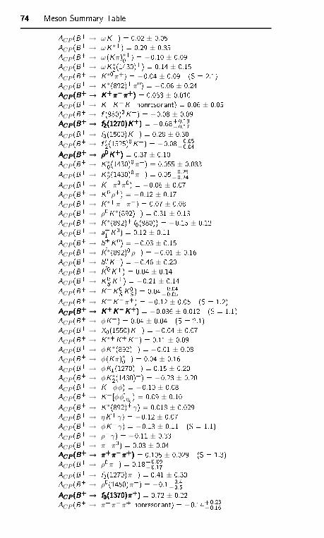
74747474 Meson Summary TableACP (B+ → ωK+) = 0.02 ± 0.05ACP (B+ → ωK∗+) = 0.29 ± 0.35ACP (B+ → ω (Kπ)∗+0 ) = −0.10 ± 0.09ACP (B+ → ωK∗2(1430)+) = 0.14 ± 0.15ACP (B+ → K∗0π+) = −0.04 ± 0.09 (S = 2.1)ACP (B+ → K∗(892)+π0) = −0.06 ± 0.24ACP (B+ → K+π−π+)ACP (B+ → K+π−π+)ACP (B+ → K+π−π+)ACP (B+ → K+π−π+) = 0.033 ± 0.010ACP (B+ → K+K−K+nonresonant) = 0.06 ± 0.05ACP (B+ → f (980)0K+) = −0.08 ± 0.09ACP (B+ → f2(1270)K+)ACP (B+ → f2(1270)K+)ACP (B+ → f2(1270)K+)ACP (B+ → f2(1270)K+) = −0.68+0.19−0.17ACP (B+ → f0(1500)K+) = 0.28 ± 0.30ACP (B+ → f ′2(1525)0K+) = −0.08+0.05−0.04ACP (B+ → ρ0K+)ACP (B+ → ρ0K+)ACP (B+ → ρ0K+)ACP (B+ → ρ0K+) = 0.37 ± 0.10ACP (B+ → K∗0(1430)0π+) = 0.055 ± 0.033ACP (B+ → K∗2(1430)0π+) = 0.05+0.29
−0.24ACP (B+ → K+π0π0) = −0.06 ± 0.07ACP (B+ → K0 ρ+) = −0.12 ± 0.17ACP (B+ → K∗+π+π−) = 0.07 ± 0.08ACP (B+ → ρ0K∗(892)+) = 0.31 ± 0.13ACP (B+ → K∗(892)+ f0(980)) = −0.15 ± 0.12ACP (B+ → a+1 K0) = 0.12 ± 0.11ACP (B+ → b+1 K0) = −0.03 ± 0.15ACP (B+ → K∗(892)0 ρ+) = −0.01 ± 0.16ACP (B+ → b01K+) = −0.46 ± 0.20ACP (B+ → K0K+) = 0.04 ± 0.14ACP (B+ → K0S K+) = −0.21 ± 0.14ACP (B+ → K+K0S K0S ) = 0.04+0.04−0.05ACP (B+ → K+K−π+) = −0.12 ± 0.05 (S = 1.2)ACP (B+ → K+K−K+)ACP (B+ → K+K−K+)ACP (B+ → K+K−K+)ACP (B+ → K+K−K+) = −0.036 ± 0.012 (S = 1.1)ACP (B+ → φK+) = 0.04 ± 0.04 (S = 2.1)ACP (B+ → X0(1550)K+) = −0.04 ± 0.07ACP (B+ → K∗+K+K−) = 0.11 ± 0.09ACP (B+ → φK∗(892)+) = −0.01 ± 0.08ACP (B+ → φ(Kπ)∗+0 ) = 0.04 ± 0.16ACP (B+ → φK1(1270)+) = 0.15 ± 0.20ACP (B+ → φK∗2(1430)+) = −0.23 ± 0.20ACP (B+ → K+φφ) = −0.10 ± 0.08ACP (B+ → K+[φφη ) = 0.09 ± 0.10ACP (B+ → K∗(892)+ γ) = 0.018 ± 0.029ACP (B+ → ηK+ γ) = −0.12 ± 0.07ACP (B+ → φK+ γ) = −0.13 ± 0.11 (S = 1.1)ACP (B+ → ρ+γ) = −0.11 ± 0.33ACP (B+ → π+π0) = 0.03 ± 0.04ACP (B+ → π+π−π+)ACP (B+ → π+π−π+)ACP (B+ → π+π−π+)ACP (B+ → π+π−π+) = 0.105 ± 0.029 (S = 1.3)ACP (B+ → ρ0π+) = 0.18+0.09
−0.17ACP (B+ → f2(1270)π+) = 0.41 ± 0.30ACP (B+ → ρ0(1450)π+) = −0.1+0.4−0.5ACP (B+ → f0(1370)π+)ACP (B+ → f0(1370)π+)ACP (B+ → f0(1370)π+)ACP (B+ → f0(1370)π+) = 0.72 ± 0.22ACP (B+ → π+π−π+ nonresonant) = −0.14+0.23
−0.16
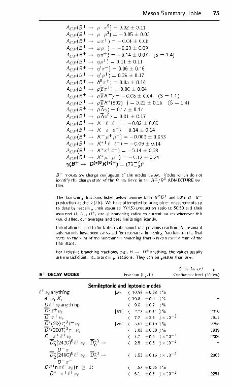
Meson Summary Table 75757575ACP (B+ → ρ+π0) = 0.02 ± 0.11ACP (B+ → ρ+ρ0) = −0.05 ± 0.05ACP (B+ → ωπ+) = −0.04 ± 0.06ACP (B+ → ωρ+) = −0.20 ± 0.09ACP (B+ → ηπ+) = −0.14 ± 0.07 (S = 1.4)ACP (B+ → ηρ+) = 0.11 ± 0.11ACP (B+ → η′π+) = 0.06 ± 0.16ACP (B+ → η′ρ+) = 0.26 ± 0.17ACP (B+ → b01π+) = 0.05 ± 0.16ACP (B+ → ppπ+) = 0.00 ± 0.04ACP (B+ → ppK+) = −0.08 ± 0.04 (S = 1.1)ACP (B+ → ppK∗(892)+) = 0.21 ± 0.16 (S = 1.4)ACP (B+ → pγ) = 0.17 ± 0.17ACP (B+ → pπ0) = 0.01 ± 0.17ACP (B+ → K+ ℓ+ ℓ−) = −0.02 ± 0.08ACP (B+ → K+ e+ e−) = 0.14 ± 0.14ACP (B+ → K+µ+µ−) = −0.003 ± 0.033ACP (B+ → K∗+ ℓ+ ℓ−) = −0.09 ± 0.14ACP (B+ → K∗ e+ e−) = −0.14 ± 0.23ACP (B+ → K∗µ+µ−) = −0.12 ± 0.24γ(B+ → D(∗)0K (∗)+)γ(B+ → D(∗)0K (∗)+)γ(B+ → D(∗)0K (∗)+)γ(B+ → D(∗)0K (∗)+) = (73+7
−9)B− modes are harge onjugates of the modes below. Modes whi h do notidentify the harge state of the B are listed in the B±/B0 ADMIXTURE se -tion.The bran hing fra tions listed below assume 50% B0B0 and 50% B+B−produ tion at the (4S). We have attempted to bring older measurements upto date by res aling their assumed (4S) produ tion ratio to 50:50 and theirassumed D, Ds , D∗, and ψ bran hing ratios to urrent values whenever thiswould ae t our averages and best limits signi antly.Indentation is used to indi ate a sub hannel of a previous rea tion. All resonantsub hannels have been orre ted for resonan e bran hing fra tions to the nalstate so the sum of the sub hannel bran hing fra tions an ex eed that of thenal state.For in lusive bran hing fra tions, e.g., B → D± anything, the values usuallyare multipli ities, not bran hing fra tions. They an be greater than one.S ale fa tor/ pB+ DECAY MODESB+ DECAY MODESB+ DECAY MODESB+ DECAY MODES Fra tion (i /) Conden e level (MeV/ )Semileptoni and leptoni modesSemileptoni and leptoni modesSemileptoni and leptoni modesSemileptoni and leptoni modesℓ+νℓ anything [sss ( 10.99 ±0.28 ) % e+ νe X ( 10.8 ±0.4 ) % D ℓ+νℓ anything ( 9.8 ±0.7 ) % D0 ℓ+νℓ [sss ( 2.27 ±0.11 ) % 2310D0 τ+ ντ ( 7.7 ±2.5 )× 10−3 1911D∗(2007)0 ℓ+νℓ [sss ( 5.69 ±0.19 ) % 2258D∗(2007)0 τ+ ντ ( 1.88 ±0.20 ) % 1839D−π+ ℓ+νℓ ( 4.2 ±0.5 )× 10−3 2306D∗0(2420)0 ℓ+νℓ, D∗00 →D−π+ ( 2.5 ±0.5 )× 10−3 D∗2(2460)0 ℓ+νℓ, D∗02 →D−π+ ( 1.53 ±0.16 )× 10−3 2065D(∗) nπℓ+ νℓ (n ≥ 1) ( 1.87 ±0.26 ) % D∗−π+ ℓ+νℓ ( 6.1 ±0.6 )× 10−3 2254
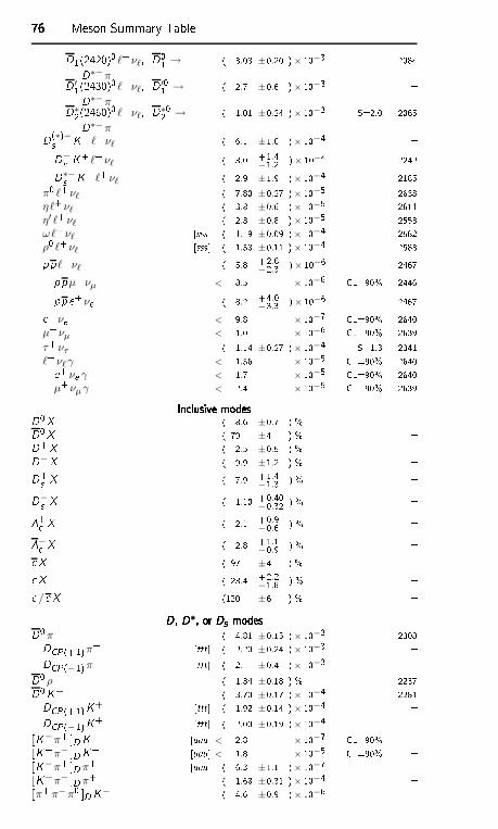
76767676 Meson Summary TableD1(2420)0 ℓ+νℓ, D01 →D∗−π+ ( 3.03 ±0.20 )× 10−3 2084D ′1(2430)0 ℓ+νℓ, D ′01 →D∗−π+ ( 2.7 ±0.6 )× 10−3 D∗2(2460)0 ℓ+νℓ, D∗02 →D∗−π+ ( 1.01 ±0.24 )× 10−3 S=2.0 2065D(∗)−s K+ ℓ+νℓ ( 6.1 ±1.0 )× 10−4 D−s K+ ℓ+νℓ ( 3.0 +1.4−1.2 )× 10−4 2242D∗−s K+ ℓ+νℓ ( 2.9 ±1.9 )× 10−4 2185
π0 ℓ+νℓ ( 7.80 ±0.27 )× 10−5 2638ηℓ+ νℓ ( 3.8 ±0.6 )× 10−5 2611η′ ℓ+νℓ ( 2.3 ±0.8 )× 10−5 2553ωℓ+νℓ [sss ( 1.19 ±0.09 )× 10−4 2582ρ0 ℓ+νℓ [sss ( 1.58 ±0.11 )× 10−4 2583pp ℓ+νℓ ( 5.8 +2.6
−2.3 )× 10−6 2467ppµ+νµ < 8.5 × 10⁻⁶ CL=90% 2446pp e+νe ( 8.2 +4.0−3.3 )× 10−6 2467e+ νe < 9.8 × 10⁻⁷ CL=90% 2640
µ+νµ < 1.0 × 10⁻⁶ CL=90% 2639τ+ ντ ( 1.14 ±0.27 )× 10−4 S=1.3 2341ℓ+νℓγ < 1.56 × 10⁻⁵ CL=90% 2640e+ νe γ < 1.7 × 10⁻⁵ CL=90% 2640
µ+νµ γ < 2.4 × 10⁻⁵ CL=90% 2639In lusive modesIn lusive modesIn lusive modesIn lusive modesD0X ( 8.6 ±0.7 ) % D0X ( 79 ±4 ) % D+X ( 2.5 ±0.5 ) % D−X ( 9.9 ±1.2 ) % D+s X ( 7.9 +1.4−1.3 ) % D−s X ( 1.10 +0.40−0.32 ) % + X ( 2.1 +0.9−0.6 ) % − X ( 2.8 +1.1−0.9 ) % X ( 97 ±4 ) % X ( 23.4 +2.2−1.8 ) % / X (120 ±6 ) % D, D∗, or Ds modesD, D∗, or Ds modesD, D∗, or Ds modesD, D∗, or Ds modesD0π+ ( 4.81 ±0.15 )× 10−3 2308DCP(+1)π+ [ttt ( 2.20 ±0.24 )× 10−3 DCP(−1)π+ [ttt ( 2.1 ±0.4 )× 10−3 D0 ρ+ ( 1.34 ±0.18 ) % 2237D0K+ ( 3.70 ±0.17 )× 10−4 2281DCP(+1)K+ [ttt ( 1.92 ±0.14 )× 10−4 DCP(−1)K+ [ttt ( 2.00 ±0.19 )× 10−4 [K−π+ DK+ [uuu < 2.8 × 10⁻⁷ CL=90% [K+π− DK+ [uuu < 1.8 × 10⁻⁵ CL=90% [K−π+ D π+ [uuu ( 6.3 ±1.1 )× 10−7 [K+π− D π+ ( 1.68 ±0.31 )× 10−4 [π+π−π0 DK− ( 4.6 ±0.9 )× 10−6
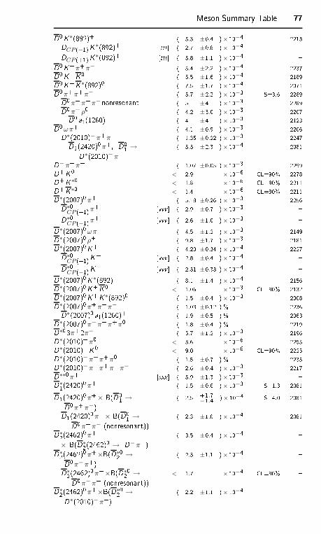
Meson Summary Table 77777777D0K∗(892)+ ( 5.3 ±0.4 )× 10−4 2213DCP (−1)K∗(892)+ [ttt ( 2.7 ±0.8 )× 10−4 DCP (+1)K∗(892)+ [ttt ( 5.8 ±1.1 )× 10−4 D0K+π+π− ( 5.4 ±2.2 )× 10−4 2237D0K+K0 ( 5.5 ±1.6 )× 10−4 2189D0K+K∗(892)0 ( 7.5 ±1.7 )× 10−4 2071D0π+π+π− ( 5.7 ±2.2 )× 10−3 S=3.6 2289D0π+π+π− nonresonant ( 5 ±4 )× 10−3 2289D0π+ ρ0 ( 4.2 ±3.0 )× 10−3 2207D0 a1(1260)+ ( 4 ±4 )× 10−3 2123D0ωπ+ ( 4.1 ±0.9 )× 10−3 2206D∗(2010)−π+π+ ( 1.35 ±0.22 )× 10−3 2247D1(2420)0π+, D01 →D∗(2010)−π+ ( 5.3 ±2.3 )× 10−4 2081D−π+π+ ( 1.07 ±0.05 )× 10−3 2299D+K0 < 2.9 × 10⁻⁶ CL=90% 2278D+K∗0 < 1.8 × 10⁻⁶ CL=90% 2211D+K∗0 < 1.4 × 10⁻⁶ CL=90% 2211D∗(2007)0π+ ( 5.18 ±0.26 )× 10−3 2256D∗0CP (+1)π+ [vvv ( 2.9 ±0.7 )× 10−3 D∗0CP (−1)π+ [vvv ( 2.6 ±1.0 )× 10−3 D∗(2007)0ωπ+ ( 4.5 ±1.2 )× 10−3 2149D∗(2007)0 ρ+ ( 9.8 ±1.7 )× 10−3 2181D∗(2007)0K+ ( 4.20 ±0.34 )× 10−4 2227D∗0CP (+1)K+ [vvv ( 2.8 ±0.4 )× 10−4 D∗0CP (−1)K+ [vvv ( 2.31 ±0.33 )× 10−4 D∗(2007)0K∗(892)+ ( 8.1 ±1.4 )× 10−4 2156D∗(2007)0K+K0 < 1.06 × 10⁻³ CL=90% 2132D∗(2007)0K+K∗(892)0 ( 1.5 ±0.4 )× 10−3 2008D∗(2007)0π+π+π− ( 1.03 ±0.12 ) % 2236D∗(2007)0 a1(1260)+ ( 1.9 ±0.5 ) % 2063D∗(2007)0π−π+π+π0 ( 1.8 ±0.4 ) % 2219D∗0 3π+ 2π− ( 5.7 ±1.2 )× 10−3 2196D∗(2010)+π0 < 3.6 × 10⁻⁶ 2255D∗(2010)+K0 < 9.0 × 10⁻⁶ CL=90% 2225D∗(2010)−π+π+π0 ( 1.5 ±0.7 ) % 2235D∗(2010)−π+π+π+π− ( 2.6 ±0.4 )× 10−3 2217D∗∗0π+ [xxx ( 5.9 ±1.3 )× 10−3 D∗1(2420)0π+ ( 1.5 ±0.6 )× 10−3 S=1.3 2081D1(2420)0π+× B(D01 →D0π+π−) ( 2.5 +1.7
−1.4 )× 10−4 S=4.0 2081D1(2420)0π+× B(D01 →D0π+π− (nonresonant)) ( 2.3 ±1.0 )× 10−4 2081D∗2(2462)0π+× B(D∗2(2462)0 → D−π+) ( 3.5 ±0.4 )× 10−4 D∗2(2462)0π+×B(D∗02 →D0π−π+) ( 2.3 ±1.1 )× 10−4 D∗2(2462)0π+×B(D∗02 →D0π−π+ (nonresonant)) < 1.7 × 10⁻⁴ CL=90% D∗2(2462)0π+×B(D∗02 →D∗(2010)−π+) ( 2.2 ±1.1 )× 10−4
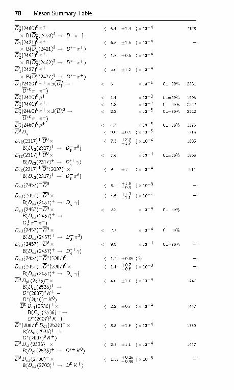
78787878 Meson Summary TableD∗0(2400)0π+× B(D∗0(2400)0 → D−π+) ( 6.4 ±1.4 )× 10−4 2128D1(2421)0π+× B(D1(2421)0 → D∗−π+) ( 6.8 ±1.5 )× 10−4 D∗2(2462)0π+× B(D∗2(2462)0 → D∗−π+) ( 1.8 ±0.5 )× 10−4 D ′1(2427)0π+× B(D ′1(2427)0 → D∗−π+) ( 5.0 ±1.2 )× 10−4 D1(2420)0π+×B(D01 →D∗0π+π−) < 6 × 10⁻⁶ CL=90% 2081D∗1(2420)0 ρ+ < 1.4 × 10⁻³ CL=90% 1996D∗2(2460)0π+ < 1.3 × 10⁻³ CL=90% 2062D∗2(2460)0π+×B(D∗02 →D∗0π+π−) < 2.2 × 10⁻⁵ CL=90% 2062D∗2(2460)0 ρ+ < 4.7 × 10⁻³ CL=90% 1976D0D+s ( 9.0 ±0.9 )× 10−3 1815Ds0(2317)+D0×B(Ds0(2317)+ → D+s π0) ( 7.3 +2.2
−1.7 )× 10−4 1605Ds0(2317)+D0×B(Ds0(2317)+ → D∗+s γ) < 7.6 × 10⁻⁴ CL=90% 1605Ds0(2317)+D∗(2007)0×B(Ds0(2317)+ → D+s π0) ( 9 ±7 )× 10−4 1511DsJ (2457)+D0 ( 3.1 +1.0−0.9 )× 10−3 DsJ (2457)+D0×B(DsJ (2457)+ → D+s γ) ( 4.6 +1.3−1.1 )× 10−4 DsJ (2457)+D0×B(DsJ (2457)+ →D+s π+π−) < 2.2 × 10⁻⁴ CL=90% DsJ (2457)+D0×B(DsJ (2457)+ → D+s π0) < 2.7 × 10⁻⁴ CL=90% DsJ (2457)+D0×B(DsJ (2457)+ → D∗+s γ) < 9.8 × 10⁻⁴ CL=90% DsJ (2457)+D∗(2007)0 ( 1.20 ±0.30 ) % DsJ (2457)+D∗(2007)0×B(DsJ (2457)+ → D+s γ) ( 1.4 +0.7−0.6 )× 10−3 D0Ds1(2536)+×B(Ds1(2536)+ →D∗(2007)0K+ +D∗(2010)+K0) ( 4.0 ±1.0 )× 10−4 1447D0Ds1(2536)+×B(Ds1(2536)+ →D∗(2007)0K+) ( 2.2 ±0.7 )× 10−4 1447D∗(2007)0Ds1(2536)+×B(Ds1(2536)+ →D∗(2007)0K+) ( 5.5 ±1.6 )× 10−4 1339D0Ds1(2536)+×B(Ds1(2536)+ → D∗+K0) ( 2.3 ±1.1 )× 10−4 1447D0DsJ (2700)+×B(DsJ (2700)+ → D0K+) ( 1.13 +0.26−0.40 )× 10−3
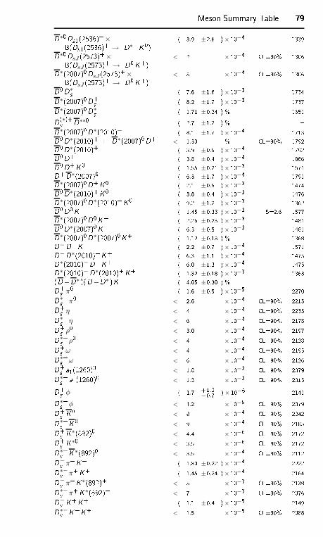
Meson Summary Table 79797979D∗0Ds1(2536)+×B(Ds1(2536)+ → D∗+K0) ( 3.9 ±2.6 )× 10−4 1339D∗0DsJ (2573)+×B(DsJ (2573)+ → D0K+) < 2 × 10⁻⁴ CL=90% 1306D∗(2007)0DsJ (2573)+×B(DsJ (2573)+ → D0K+) < 5 × 10⁻⁴ CL=90% 1306D0D∗+s ( 7.6 ±1.6 )× 10−3 1734D∗(2007)0D+s ( 8.2 ±1.7 )× 10−3 1737D∗(2007)0D∗+s ( 1.71 ±0.24 ) % 1651D(∗)+s D∗∗0 ( 2.7 ±1.2 ) % D∗(2007)0D∗(2010)+ ( 8.1 ±1.7 )× 10−4 1713D0D∗(2010)+ + D∗(2007)0D+ < 1.30 % CL=90% 1792D0D∗(2010)+ ( 3.9 ±0.5 )× 10−4 1792D0D+ ( 3.8 ±0.4 )× 10−4 1866D0D+K0 ( 1.55 ±0.21 )× 10−3 1571D+D∗(2007)0 ( 6.3 ±1.7 )× 10−4 1791D∗(2007)0D+K0 ( 2.1 ±0.5 )× 10−3 1474D0D∗(2010)+K0 ( 3.8 ±0.4 )× 10−3 1476D∗(2007)0D∗(2010)+K0 ( 9.2 ±1.2 )× 10−3 1362D0D0K+ ( 1.45 ±0.33 )× 10−3 S=2.6 1577D∗(2007)0D0K+ ( 2.26 ±0.23 )× 10−3 1481D0D∗(2007)0K+ ( 6.3 ±0.5 )× 10−3 1481D∗(2007)0D∗(2007)0K+ ( 1.12 ±0.13 ) % 1368D−D+K+ ( 2.2 ±0.7 )× 10−4 1571D−D∗(2010)+K+ ( 6.3 ±1.1 )× 10−4 1475D∗(2010)−D+K+ ( 6.0 ±1.3 )× 10−4 1475D∗(2010)−D∗(2010)+K+ ( 1.32 ±0.18 )× 10−3 1363(D+D∗ )(D+D∗ )K ( 4.05 ±0.30 ) % D+s π0 ( 1.6 ±0.5 )× 10−5 2270D∗+s π0 < 2.6 × 10⁻⁴ CL=90% 2215D+s η < 4 × 10⁻⁴ CL=90% 2235D∗+s η < 6 × 10⁻⁴ CL=90% 2178D+s ρ0 < 3.0 × 10⁻⁴ CL=90% 2197D∗+s ρ0 < 4 × 10⁻⁴ CL=90% 2138D+s ω < 4 × 10⁻⁴ CL=90% 2195D∗+s ω < 6 × 10⁻⁴ CL=90% 2136D+s a1(1260)0 < 1.8 × 10⁻³ CL=90% 2079D∗+s a1(1260)0 < 1.3 × 10⁻³ CL=90% 2015D+s φ ( 1.7 +1.2−0.7 )× 10−6 2141D∗+s φ < 1.2 × 10⁻⁵ CL=90% 2079D+s K0 < 8 × 10⁻⁴ CL=90% 2242D∗+s K0 < 9 × 10⁻⁴ CL=90% 2185D+s K∗(892)0 < 4.4 × 10⁻⁶ CL=90% 2172D+s K∗0 < 3.5 × 10⁻⁶ CL=90% 2172D∗+s K∗(892)0 < 3.5 × 10⁻⁴ CL=90% 2112D−s π+K+ ( 1.80 ±0.22 )× 10−4 2222D∗−s π+K+ ( 1.45 ±0.24 )× 10−4 2164D−s π+K∗(892)+ < 5 × 10⁻³ CL=90% 2138D∗−s π+K∗(892)+ < 7 × 10⁻³ CL=90% 2076D−s K+K+ ( 1.1 ±0.4 )× 10−5 2149D∗−s K+K+ < 1.5 × 10⁻⁵ CL=90% 2088
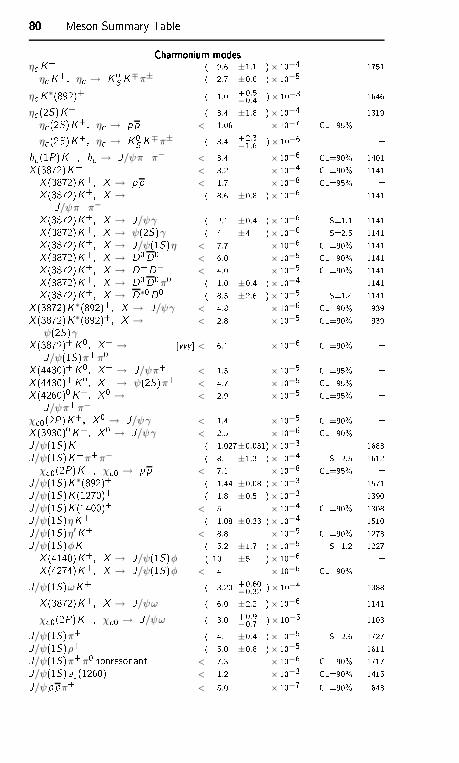
80808080 Meson Summary TableCharmonium modesCharmonium modesCharmonium modesCharmonium modesη K+ ( 9.6 ±1.1 )× 10−4 1751
η K+, η → K0S K∓π± ( 2.7 ±0.6 )× 10−5 η K∗(892)+ ( 1.0 +0.5
−0.4 )× 10−3 1646η (2S)K+ ( 3.4 ±1.8 )× 10−4 1319
η (2S)K+, η → pp < 1.06 × 10⁻⁷ CL=95% η (2S)K+, η → K0S K∓π± ( 3.4 +2.3
−1.6 )× 10−6 h (1P)K+, h → J/ψπ+π− < 3.4 × 10⁻⁶ CL=90% 1401X (3872)K+ < 3.2 × 10⁻⁴ CL=90% 1141X (3872)K+, X → pp < 1.7 × 10⁻⁸ CL=95% X (3872)K+, X →J/ψπ+π−( 8.6 ±0.8 )× 10−6 1141X (3872)K+, X → J/ψγ ( 2.1 ±0.4 )× 10−6 S=1.1 1141X (3872)K+, X → ψ(2S)γ ( 4 ±4 )× 10−6 S=2.5 1141X (3872)K+, X → J/ψ(1S)η < 7.7 × 10⁻⁶ CL=90% 1141X (3872)K+, X → D0D0 < 6.0 × 10⁻⁵ CL=90% 1141X (3872)K+, X → D+D− < 4.0 × 10⁻⁵ CL=90% 1141X (3872)K+, X → D0D0π0 ( 1.0 ±0.4 )× 10−4 1141X (3872)K+, X → D∗0D0 ( 8.5 ±2.6 )× 10−5 S=1.4 1141X (3872)K∗(892)+, X → J/ψγ < 4.8 × 10⁻⁶ CL=90% 939X (3872)K∗(892)+, X →
ψ(2S)γ < 2.8 × 10⁻⁵ CL=90% 939X (3872)+K0, X+ →J/ψ(1S)π+π0 [yyy < 6.1 × 10⁻⁶ CL=90% X (4430)+K0, X+ → J/ψπ+ < 1.5 × 10⁻⁵ CL=95% X (4430)+K0, X+ → ψ(2S)π+ < 4.7 × 10⁻⁵ CL=95% X (4260)0K+, X 0 →J/ψπ+π−< 2.9 × 10⁻⁵ CL=95%
χ 0(2P)K+, X 0 → J/ψγ < 1.4 × 10⁻⁵ CL=90% X (3930)0K+, X 0 → J/ψγ < 2.5 × 10⁻⁶ CL=90% J/ψ(1S)K+ ( 1.027±0.031)× 10−3 1683J/ψ(1S)K+π+π− ( 8.1 ±1.3 )× 10−4 S=2.5 1612χ 0(2P)K+, χ 0 → pp < 7.1 × 10⁻⁸ CL=95% J/ψ(1S)K∗(892)+ ( 1.44 ±0.08 )× 10−3 1571J/ψ(1S)K (1270)+ ( 1.8 ±0.5 )× 10−3 1390J/ψ(1S)K (1400)+ < 5 × 10⁻⁴ CL=90% 1308J/ψ(1S)ηK+ ( 1.08 ±0.33 )× 10−4 1510J/ψ(1S)η′K+ < 8.8 × 10⁻⁵ CL=90% 1273J/ψ(1S)φK+ ( 5.2 ±1.7 )× 10−5 S=1.2 1227X (4140)K+, X → J/ψ(1S)φ ( 10 ±5 )× 10−6 X (4274)K+, X → J/ψ(1S)φ < 4 × 10⁻⁶ CL=90% J/ψ(1S)ωK+ ( 3.20 +0.60
−0.32 )× 10−4 1388X (3872)K+, X → J/ψω ( 6.0 ±2.2 )× 10−6 1141χ 0(2P)K+, χ 0 → J/ψω ( 3.0 +0.9
−0.7 )× 10−5 1103J/ψ(1S)π+ ( 4.1 ±0.4 )× 10−5 S=2.6 1727J/ψ(1S)ρ+ ( 5.0 ±0.8 )× 10−5 1611J/ψ(1S)π+π0 nonresonant < 7.3 × 10⁻⁶ CL=90% 1717J/ψ(1S)a1(1260)+ < 1.2 × 10⁻³ CL=90% 1415J/ψppπ+ < 5.0 × 10⁻⁷ CL=90% 643
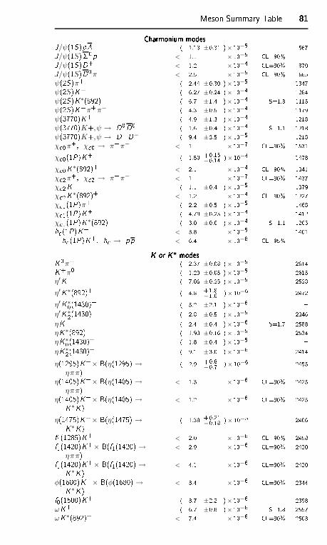
Meson Summary Table 81818181Charmonium modesCharmonium modesCharmonium modesCharmonium modesJ/ψ(1S)p ( 1.18 ±0.31 )× 10−5 567J/ψ(1S)0p < 1.1 × 10⁻⁵ CL=90% J/ψ(1S)D+ < 1.2 × 10⁻⁴ CL=90% 870J/ψ(1S)D0π+ < 2.5 × 10⁻⁵ CL=90% 665ψ(2S)π+ ( 2.44 ±0.30 )× 10−5 1347ψ(2S)K+ ( 6.27 ±0.24 )× 10−4 1284ψ(2S)K∗(892)+ ( 6.7 ±1.4 )× 10−4 S=1.3 1115ψ(2S)K+π+π− ( 4.3 ±0.5 )× 10−4 1179ψ(3770)K+ ( 4.9 ±1.3 )× 10−4 1218ψ(3770)K+,ψ → D0D0 ( 1.6 ±0.4 )× 10−4 S=1.1 1218ψ(3770)K+,ψ → D+D− ( 9.4 ±3.5 )× 10−5 1218χ 0π+, χ 0 → π+π− < 1 × 10⁻⁷ CL=90% 1531χ 0(1P)K+ ( 1.50 +0.15
−0.14 )× 10−4 1478χ 0K∗(892)+ < 2.1 × 10⁻⁴ CL=90% 1341χ 2π+, χ 2 → π+π− < 1 × 10⁻⁷ CL=90% 1437χ 2K+ ( 1.1 ±0.4 )× 10−5 1379χ 2K∗(892)+ < 1.2 × 10⁻⁴ CL=90% 1227χ 1(1P)π+ ( 2.2 ±0.5 )× 10−5 1468χ 1(1P)K+ ( 4.79 ±0.23 )× 10−4 1412χ 1(1P)K∗(892)+ ( 3.0 ±0.6 )× 10−4 S=1.1 1265h (1P)K+ < 3.8 × 10⁻⁵ 1401h (1P)K+, h → pp < 6.4 × 10⁻⁸ CL=95% K or K∗ modesK or K∗ modesK or K∗ modesK or K∗ modesK0π+ ( 2.37 ±0.08 )× 10−5 2614K+π0 ( 1.29 ±0.05 )× 10−5 2615η′K+ ( 7.06 ±0.25 )× 10−5 2528η′K∗(892)+ ( 4.8 +1.8
−1.6 )× 10−6 2472η′K∗0(1430)+ ( 5.2 ±2.1 )× 10−6 η′K∗2(1430)+ ( 2.8 ±0.5 )× 10−5 2346ηK+ ( 2.4 ±0.4 )× 10−6 S=1.7 2588ηK∗(892)+ ( 1.93 ±0.16 )× 10−5 2534ηK∗0(1430)+ ( 1.8 ±0.4 )× 10−5 ηK∗2(1430)+ ( 9.1 ±3.0 )× 10−6 2414η(1295)K+× B(η(1295) →
ηππ) ( 2.9 +0.8−0.7 )× 10−6 2455
η(1405)K+× B(η(1405) →ηππ) < 1.3 × 10⁻⁶ CL=90% 2425
η(1405)K+× B(η(1405) →K∗K ) < 1.2 × 10⁻⁶ CL=90% 2425η(1475)K+× B(η(1475) →K∗K ) ( 1.38 +0.21
−0.18 )× 10−5 2406f1(1285)K+ < 2.0 × 10⁻⁶ CL=90% 2458f1(1420)K+× B(f1(1420) →ηππ) < 2.9 × 10⁻⁶ CL=90% 2420f1(1420)K+× B(f1(1420) →K∗K ) < 4.1 × 10⁻⁶ CL=90% 2420
φ(1680)K+× B(φ(1680) →K∗K ) < 3.4 × 10⁻⁶ CL=90% 2344f0(1500)K+ ( 3.7 ±2.2 )× 10−6 2398ωK+ ( 6.7 ±0.8 )× 10−6 S=1.8 2557ωK∗(892)+ < 7.4 × 10⁻⁶ CL=90% 2503
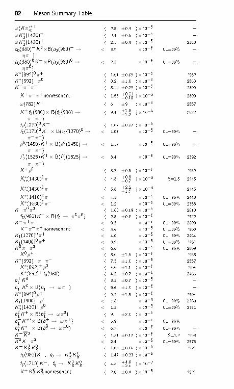
82828282 Meson Summary Tableω (Kπ)∗+0 ( 2.8 ±0.4 )× 10−5 ωK∗0(1430)+ ( 2.4 ±0.5 )× 10−5 ωK∗2(1430)+ ( 2.1 ±0.4 )× 10−5 2380a0(980)+K0×B(a0(980)+ →
ηπ+) < 3.9 × 10⁻⁶ CL=90% a0(980)0K+×B(a0(980)0 →ηπ0) < 2.5 × 10⁻⁶ CL=90% K∗(892)0π+ ( 1.01 ±0.09 )× 10−5 2562K∗(892)+π0 ( 8.2 ±1.9 )× 10−6 2563K+π−π+ ( 5.10 ±0.29 )× 10−5 2609K+π−π+nonresonant ( 1.63 +0.21
−0.15 )× 10−5 2609ω(782)K+ ( 6 ±9 )× 10−6 2557K+ f0(980)× B(f0(980) →
π+π−) ( 9.4 +1.0−1.2 )× 10−6 2522f2(1270)0K+ ( 1.07 ±0.27 )× 10−6 f0(1370)0K+× B(f0(1370)0 →
π+π−) < 1.07 × 10⁻⁵ CL=90% ρ0(1450)K+× B(ρ0(1450) →
π+π−) < 1.17 × 10⁻⁵ CL=90% f ′2(1525)K+× B(f ′2(1525) →π+π−) < 3.4 × 10⁻⁶ CL=90% 2392K+ρ0 ( 3.7 ±0.5 )× 10−6 2559K∗0(1430)0π+ ( 4.5 +0.9
−0.7 )× 10−5 S=1.5 2445K∗2(1430)0π+ ( 5.6 +2.2−1.5 )× 10−6 2445K∗(1410)0π+ < 4.5 × 10⁻⁵ CL=90% 2448K∗(1680)0π+ < 1.2 × 10⁻⁵ CL=90% 2358K+π0π0 ( 1.62 ±0.19 )× 10−5 2610f0(980)K+× B(f0 → π0π0) ( 2.8 ±0.8 )× 10−6 2522K−π+π+ < 9.5 × 10⁻⁷ CL=90% 2609K−π+π+nonresonant < 5.6 × 10⁻⁵ CL=90% 2609K1(1270)0π+ < 4.0 × 10⁻⁵ CL=90% 2484K1(1400)0π+ < 3.9 × 10⁻⁵ CL=90% 2451K0π+π0 < 6.6 × 10⁻⁵ CL=90% 2609K0ρ+ ( 8.0 ±1.5 )× 10−6 2558K∗(892)+π+π− ( 7.5 ±1.0 )× 10−5 2557K∗(892)+ ρ0 ( 4.6 ±1.1 )× 10−6 2504K∗(892)+ f0(980) ( 4.2 ±0.7 )× 10−6 2466a+1 K0 ( 3.5 ±0.7 )× 10−5 b+1 K0× B(b+1 → ωπ+) ( 9.6 ±1.9 )× 10−6 K∗(892)0 ρ+ ( 9.2 ±1.5 )× 10−6 2504K1(1400)+ρ0 < 7.8 × 10⁻⁴ CL=90% 2388K∗2(1430)+ρ0 < 1.5 × 10⁻³ CL=90% 2381b01K+× B(b01 → ωπ0) ( 9.1 ±2.0 )× 10−6 b+1 K∗0× B(b+1 → ωπ+) < 5.9 × 10⁻⁶ CL=90% b01K∗+× B(b01 → ωπ0) < 6.7 × 10⁻⁶ CL=90% K+K0 ( 1.31 ±0.17 )× 10−6 S=1.2 2593K0K+π0 < 2.4 × 10⁻⁵ CL=90% 2578K+K0S K0S ( 1.08 ±0.06 )× 10−5 2521f0(980)K+, f0 → K0S K0S ( 1.47 ±0.33 )× 10−5 f0(1710)K+, f0 → K0S K0S ( 4.8 +4.0−2.6 )× 10−7 K+K0S K0S nonresonant ( 2.0 ±0.4 )× 10−5 2521
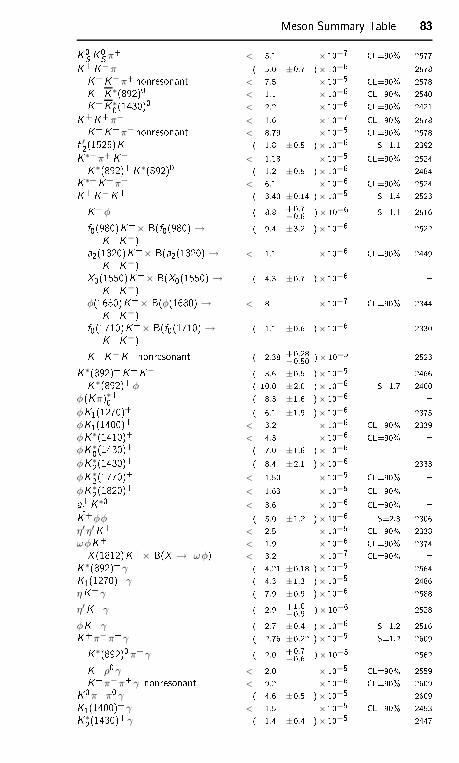
Meson Summary Table 83838383K0S K0S π+ < 5.1 × 10⁻⁷ CL=90% 2577K+K−π+ ( 5.0 ±0.7 )× 10−6 2578K+K−π+ nonresonant < 7.5 × 10⁻⁵ CL=90% 2578K+K∗(892)0 < 1.1 × 10⁻⁶ CL=90% 2540K+K∗0(1430)0 < 2.2 × 10⁻⁶ CL=90% 2421K+K+π− < 1.6 × 10⁻⁷ CL=90% 2578K+K+π− nonresonant < 8.79 × 10⁻⁵ CL=90% 2578f ′2(1525)K+ ( 1.8 ±0.5 )× 10−6 S=1.1 2392K∗+π+K− < 1.18 × 10⁻⁵ CL=90% 2524K∗(892)+K∗(892)0 ( 1.2 ±0.5 )× 10−6 2484K∗+K+π− < 6.1 × 10⁻⁶ CL=90% 2524K+K−K+ ( 3.40 ±0.14 )× 10−5 S=1.4 2523K+φ ( 8.8 +0.7−0.6 )× 10−6 S=1.1 2516f0(980)K+× B(f0(980) →K+K−) ( 9.4 ±3.2 )× 10−6 2522a2(1320)K+× B(a2(1320) →K+K−) < 1.1 × 10⁻⁶ CL=90% 2449X0(1550)K+× B(X0(1550) →K+K−) ( 4.3 ±0.7 )× 10−6
φ(1680)K+× B(φ(1680) →K+K−) < 8 × 10⁻⁷ CL=90% 2344f0(1710)K+× B(f0(1710) →K+K−) ( 1.1 ±0.6 )× 10−6 2330K+K−K+nonresonant ( 2.38 +0.28−0.50 )× 10−5 2523K∗(892)+K+K− ( 3.6 ±0.5 )× 10−5 2466K∗(892)+φ ( 10.0 ±2.0 )× 10−6 S=1.7 2460
φ(Kπ)∗+0 ( 8.3 ±1.6 )× 10−6 φK1(1270)+ ( 6.1 ±1.9 )× 10−6 2375φK1(1400)+ < 3.2 × 10⁻⁶ CL=90% 2339φK∗(1410)+ < 4.3 × 10⁻⁶ CL=90% φK∗0(1430)+ ( 7.0 ±1.6 )× 10−6 φK∗2(1430)+ ( 8.4 ±2.1 )× 10−6 2333φK∗2(1770)+ < 1.50 × 10⁻⁵ CL=90% φK∗2(1820)+ < 1.63 × 10⁻⁵ CL=90% a+1 K∗0 < 3.6 × 10⁻⁶ CL=90% K+φφ ( 5.0 ±1.2 )× 10−6 S=2.3 2306η′ η′K+ < 2.5 × 10⁻⁵ CL=90% 2338ωφK+ < 1.9 × 10⁻⁶ CL=90% 2374X (1812)K+× B(X → ωφ) < 3.2 × 10⁻⁷ CL=90% K∗(892)+ γ ( 4.21 ±0.18 )× 10−5 2564K1(1270)+γ ( 4.3 ±1.3 )× 10−5 2486ηK+ γ ( 7.9 ±0.9 )× 10−6 2588η′K+γ ( 2.9 +1.0
−0.9 )× 10−6 2528φK+ γ ( 2.7 ±0.4 )× 10−6 S=1.2 2516K+π−π+γ ( 2.76 ±0.22 )× 10−5 S=1.2 2609K∗(892)0π+ γ ( 2.0 +0.7
−0.6 )× 10−5 2562K+ρ0 γ < 2.0 × 10⁻⁵ CL=90% 2559K+π−π+γ nonresonant < 9.2 × 10⁻⁶ CL=90% 2609K0π+π0 γ ( 4.6 ±0.5 )× 10−5 2609K1(1400)+γ < 1.5 × 10⁻⁵ CL=90% 2453K∗2(1430)+γ ( 1.4 ±0.4 )× 10−5 2447
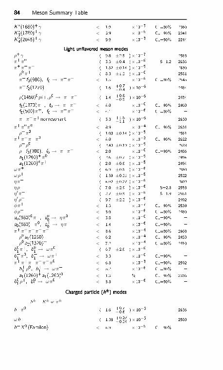
84848484 Meson Summary TableK∗(1680)+γ < 1.9 × 10⁻³ CL=90% 2360K∗3(1780)+γ < 3.9 × 10⁻⁵ CL=90% 2341K∗4(2045)+γ < 9.9 × 10⁻³ CL=90% 2244Light un avored meson modesLight un avored meson modesLight un avored meson modesLight un avored meson modesρ+γ ( 9.8 ±2.5 )× 10−7 2583π+π0 ( 5.5 ±0.4 )× 10−6 S=1.2 2636π+π+π− ( 1.52 ±0.14 )× 10−5 2630
ρ0π+ ( 8.3 ±1.2 )× 10−6 2581π+ f0(980), f0 → π+π− < 1.5 × 10⁻⁶ CL=90% 2545π+ f2(1270) ( 1.6 +0.7
−0.4 )× 10−6 2484ρ(1450)0pi+,ρ0 → π+π− ( 1.4 +0.6
−0.9 )× 10−6 2434f0(1370)π+, f0 → π+π− < 4.0 × 10⁻⁶ CL=90% 2460f0(500)π+, f0 → π+π− < 4.1 × 10⁻⁶ CL=90% π+π−π+ nonresonant ( 5.3 +1.5
−1.1 )× 10−6 2630π+π0π0 < 8.9 × 10⁻⁴ CL=90% 2631
ρ+π0 ( 1.09 ±0.14 )× 10−5 2581π+π−π+π0 < 4.0 × 10⁻³ CL=90% 2622
ρ+ρ0 ( 2.40 ±0.19 )× 10−5 2523ρ+ f0(980), f0 → π+π− < 2.0 × 10⁻⁶ CL=90% 2486a1(1260)+π0 ( 2.6 ±0.7 )× 10−5 2494a1(1260)0π+ ( 2.0 ±0.6 )× 10−5 2494
ωπ+ ( 6.9 ±0.5 )× 10−6 2580ωρ+ ( 1.59 ±0.21 )× 10−5 2522ηπ+ ( 4.02 ±0.27 )× 10−6 2609ηρ+ ( 7.0 ±2.9 )× 10−6 S=2.8 2553η′π+ ( 2.7 ±0.9 )× 10−6 S=1.9 2551η′ρ+ ( 9.7 ±2.2 )× 10−6 2492φπ+ < 1.5 × 10⁻⁷ CL=90% 2539φρ+ < 3.0 × 10⁻⁶ CL=90% 2480a0(980)0π+, a00 → ηπ0 < 5.8 × 10⁻⁶ CL=90% a0(980)+π0, a+0 → ηπ+ < 1.4 × 10⁻⁶ CL=90% π+π+π+π−π− < 8.6 × 10⁻⁴ CL=90% 2608
ρ0 a1(1260)+ < 6.2 × 10⁻⁴ CL=90% 2433ρ0 a2(1320)+ < 7.2 × 10⁻⁴ CL=90% 2410b01π+, b01 → ωπ0 ( 6.7 ±2.0 )× 10−6 b+1 π0, b+1 → ωπ+ < 3.3 × 10⁻⁶ CL=90%
π+π+π+π−π−π0 < 6.3 × 10⁻³ CL=90% 2592b+1 ρ0, b+1 → ωπ+ < 5.2 × 10⁻⁶ CL=90% a1(1260)+a1(1260)0 < 1.3 % CL=90% 2336b01 ρ+, b01 → ωπ0 < 3.3 × 10⁻⁶ CL=90% Charged parti le (h±) modesCharged parti le (h±) modesCharged parti le (h±) modesCharged parti le (h±) modesh± = K± or π±h+π0 ( 1.6 +0.7−0.6 )× 10−5 2636
ωh+ ( 1.38 +0.27−0.24 )× 10−5 2580h+X 0 (Familon) < 4.9 × 10⁻⁵ CL=90%
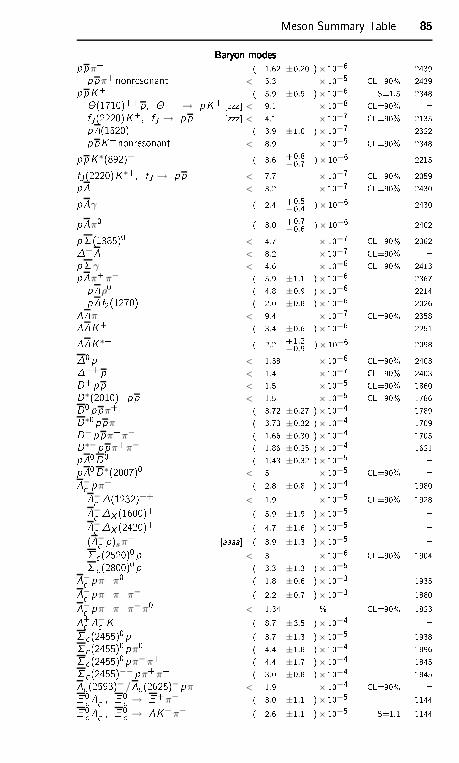
Meson Summary Table 85858585Baryon modesBaryon modesBaryon modesBaryon modesppπ+ ( 1.62 ±0.20 )× 10−6 2439ppπ+nonresonant < 5.3 × 10⁻⁵ CL=90% 2439ppK+ ( 5.9 ±0.5 )× 10−6 S=1.5 2348(1710)++p, ++ → pK+ [zzz < 9.1 × 10⁻⁸ CL=90% fJ (2220)K+, fJ → pp [zzz < 4.1 × 10⁻⁷ CL=90% 2135p(1520) ( 3.9 ±1.0 )× 10−7 2322ppK+nonresonant < 8.9 × 10⁻⁵ CL=90% 2348ppK∗(892)+ ( 3.6 +0.8−0.7 )× 10−6 2215fJ (2220)K∗+, fJ → pp < 7.7 × 10⁻⁷ CL=90% 2059p < 3.2 × 10⁻⁷ CL=90% 2430pγ ( 2.4 +0.5−0.4 )× 10−6 2430pπ0 ( 3.0 +0.7−0.6 )× 10−6 2402p (1385)0 < 4.7 × 10⁻⁷ CL=90% 2362+ < 8.2 × 10⁻⁷ CL=90% p γ < 4.6 × 10⁻⁶ CL=90% 2413pπ+π− ( 5.9 ±1.1 )× 10−6 2367pρ0 ( 4.8 ±0.9 )× 10−6 2214pf2(1270) ( 2.0 ±0.8 )× 10−6 2026π+ < 9.4 × 10⁻⁷ CL=90% 2358K+ ( 3.4 ±0.6 )× 10−6 2251K∗+ ( 2.2 +1.2−0.9 )× 10−6 20980 p < 1.38 × 10⁻⁶ CL=90% 2403++ p < 1.4 × 10⁻⁷ CL=90% 2403D+ pp < 1.5 × 10⁻⁵ CL=90% 1860D∗(2010)+ pp < 1.5 × 10⁻⁵ CL=90% 1786D0 ppπ+ ( 3.72 ±0.27 )× 10−4 1789D∗0ppπ+ ( 3.73 ±0.32 )× 10−4 1709D− ppπ+π− ( 1.66 ±0.30 )× 10−4 1705D∗−ppπ+π− ( 1.86 ±0.25 )× 10−4 1621p0D0 ( 1.43 ±0.32 )× 10−5 p0D∗(2007)0 < 5 × 10⁻⁵ CL=90% − pπ+ ( 2.8 ±0.8 )× 10−4 1980− (1232)++ < 1.9 × 10⁻⁵ CL=90% 1928− X (1600)++ ( 5.9 ±1.9 )× 10−5 − X (2420)++ ( 4.7 ±1.6 )× 10−5 (− p)sπ+ [aaaa ( 3.9 ±1.3 )× 10−5 (2520)0 p < 3 × 10⁻⁶ CL=90% 1904 (2800)0 p ( 3.3 ±1.3 )× 10−5 − pπ+π0 ( 1.8 ±0.6 )× 10−3 1935− pπ+π+π− ( 2.2 ±0.7 )× 10−3 1880− pπ+π+π−π0 < 1.34 % CL=90% 1823+ − K+ ( 8.7 ±3.5 )× 10−4 (2455)0 p ( 3.7 ±1.3 )× 10−5 1938 (2455)0 pπ0 ( 4.4 ±1.8 )× 10−4 1896 (2455)0 pπ−π+ ( 4.4 ±1.7 )× 10−4 1845 (2455)−− pπ+π+ ( 3.0 ±0.8 )× 10−4 1845 (2593)− / (2625)− pπ+ < 1.9 × 10⁻⁴ CL=90% 0 + , 0 → +π− ( 3.0 ±1.1 )× 10−5 1144 0 + , 0 → K+π− ( 2.6 ±1.1 )× 10−5 S=1.1 1144
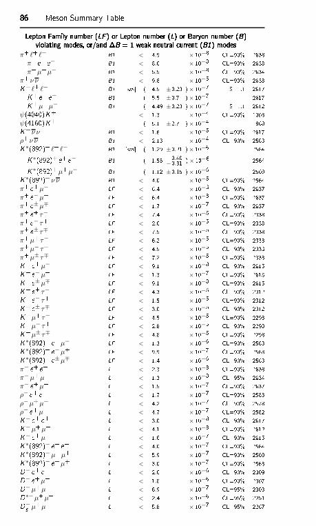
86868686 Meson Summary TableLepton Family number (LF ) or Lepton number (L) or Baryon number (B)Lepton Family number (LF ) or Lepton number (L) or Baryon number (B)Lepton Family number (LF ) or Lepton number (L) or Baryon number (B)Lepton Family number (LF ) or Lepton number (L) or Baryon number (B)violating modes, or/and B = 1 weak neutral urrent (B1) modesviolating modes, or/and B = 1 weak neutral urrent (B1) modesviolating modes, or/and B = 1 weak neutral urrent (B1) modesviolating modes, or/and B = 1 weak neutral urrent (B1) modesπ+ ℓ+ ℓ− B1 < 4.9 × 10⁻⁸ CL=90% 2638
π+ e+ e− B1 < 8.0 × 10⁻⁸ CL=90% 2638π+µ+µ− B1 < 5.5 × 10⁻⁸ CL=90% 2634
π+ ν ν B1 < 9.8 × 10⁻⁵ CL=90% 2638K+ ℓ+ ℓ− B1 [sss ( 4.51 ±0.23 ) × 10−7 S=1.1 2617K+ e+ e− B1 ( 5.5 ±0.7 ) × 10−7 2617K+µ+µ− B1 ( 4.49 ±0.23 ) × 10−7 S=1.1 2612ψ(4040)K+ < 1.3 × 10⁻⁴ CL=90% 1003ψ(4160)K+ ( 5.1 ±2.7 ) × 10−4 868K+ν ν B1 < 1.6 × 10⁻⁵ CL=90% 2617ρ+ν ν B1 < 2.13 × 10⁻⁴ CL=90% 2583K∗(892)+ ℓ+ ℓ− B1 [sss ( 1.29 ±0.21 ) × 10−6 2564K∗(892)+ e+ e− B1 ( 1.55 +0.40
−0.31 )× 10−6 2564K∗(892)+µ+µ− B1 ( 1.12 ±0.15 ) × 10−6 2560K∗(892)+ ν ν B1 < 4.0 × 10⁻⁵ CL=90% 2564π+ e+µ− LF < 6.4 × 10⁻³ CL=90% 2637π+ e−µ+ LF < 6.4 × 10⁻³ CL=90% 2637π+ e±µ∓ LF < 1.7 × 10⁻⁷ CL=90% 2637π+ e+ τ− LF < 7.4 × 10⁻⁵ CL=90% 2338π+ e− τ+ LF < 2.0 × 10⁻⁵ CL=90% 2338π+ e± τ∓ LF < 7.5 × 10⁻⁵ CL=90% 2338π+µ+ τ− LF < 6.2 × 10⁻⁵ CL=90% 2333π+µ− τ+ LF < 4.5 × 10⁻⁵ CL=90% 2333π+µ± τ∓ LF < 7.2 × 10⁻⁵ CL=90% 2333K+ e+µ− LF < 9.1 × 10⁻⁸ CL=90% 2615K+ e−µ+ LF < 1.3 × 10⁻⁷ CL=90% 2615K+ e±µ∓ LF < 9.1 × 10⁻⁸ CL=90% 2615K+ e+ τ− LF < 4.3 × 10⁻⁵ CL=90% 2312K+ e− τ+ LF < 1.5 × 10⁻⁵ CL=90% 2312K+ e± τ∓ LF < 3.0 × 10⁻⁵ CL=90% 2312K+µ+ τ− LF < 4.5 × 10⁻⁵ CL=90% 2298K+µ− τ+ LF < 2.8 × 10⁻⁵ CL=90% 2298K+µ± τ∓ LF < 4.8 × 10⁻⁵ CL=90% 2298K∗(892)+ e+µ− LF < 1.3 × 10⁻⁶ CL=90% 2563K∗(892)+ e−µ+ LF < 9.9 × 10⁻⁷ CL=90% 2563K∗(892)+ e±µ∓ LF < 1.4 × 10⁻⁶ CL=90% 2563π− e+ e+ L < 2.3 × 10⁻⁸ CL=90% 2638π−µ+µ+ L < 1.3 × 10⁻⁸ CL=95% 2634π− e+µ+ L < 1.5 × 10⁻⁷ CL=90% 2637ρ− e+ e+ L < 1.7 × 10⁻⁷ CL=90% 2583ρ−µ+µ+ L < 4.2 × 10⁻⁷ CL=90% 2578ρ− e+µ+ L < 4.7 × 10⁻⁷ CL=90% 2582K− e+ e+ L < 3.0 × 10⁻⁸ CL=90% 2617K−µ+µ+ L < 4.1 × 10⁻⁸ CL=90% 2612K− e+µ+ L < 1.6 × 10⁻⁷ CL=90% 2615K∗(892)− e+ e+ L < 4.0 × 10⁻⁷ CL=90% 2564K∗(892)−µ+µ+ L < 5.9 × 10⁻⁷ CL=90% 2560K∗(892)− e+µ+ L < 3.0 × 10⁻⁷ CL=90% 2563D− e+ e+ L < 2.6 × 10⁻⁶ CL=90% 2309D− e+µ+ L < 1.8 × 10⁻⁶ CL=90% 2307D−µ+µ+ L < 6.9 × 10⁻⁷ CL=95% 2303D∗−µ+µ+ L < 2.4 × 10⁻⁶ CL=95% 2251D−s µ+µ+ L < 5.8 × 10⁻⁷ CL=95% 2267
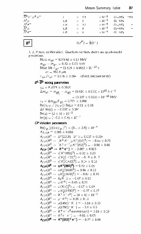
Meson Summary Table 87878787D0π−µ+µ+ L < 1.5 × 10⁻⁶ CL=95% 22950µ+ L,B < 6 × 10⁻⁸ CL=90% 0 e+ L,B < 3.2 × 10⁻⁸ CL=90% 0µ+ L,B < 6 × 10⁻⁸ CL=90% 0 e+ L,B < 8 × 10⁻⁸ CL=90% B0B0B0B0 I (JP ) = 12 (0−)I , J , P need onrmation. Quantum numbers shown are quark-modelpredi tions.Mass mB0 = 5279.58 ± 0.17 MeVmB0 − mB± = 0.32 ± 0.06 MeVMean life τB0 = (1.519 ± 0.005)× 10−12 s τ = 455.4 µmτB+/τB0 = 1.076 ± 0.004 (dire t measurements)B0-B0 mixing parametersB0-B0 mixing parametersB0-B0 mixing parametersB0-B0 mixing parametersχd = 0.1874 ± 0.0018mB0 = mB0H − mB0L = (0.510 ± 0.003)× 1012 h s−1= (3.337 ± 0.033)× 10−10 MeVxd = mB0/B0 = 0.774 ± 0.006Re(λCP /
∣
∣λCP
∣
∣
) Re(z) = 0.01 ± 0.05 Re(z) = −0.007 ± 0.004Re(z) = (2 ± 5)× 10−2Im(z) = (−0.8 ± 0.4)× 10−2CP violation parametersCP violation parametersCP violation parametersCP violation parametersRe(ǫB0)/(1+∣
∣ǫB0 ∣∣2) = (0.1 ± 0.8)× 10−3AT/CP = 0.005 ± 0.018ACP (B0 → D∗(2010)+D−) = 0.037 ± 0.034ACP (B0 → [K+K− DK∗(892)0) = −0.45 ± 0.23ACP (B0 → [K+π− DK∗(892)0) = −0.08 ± 0.08ACP (B0 → K+π−)ACP (B0 → K+π−)ACP (B0 → K+π−)ACP (B0 → K+π−) = −0.082 ± 0.006ACP (B0 → η′K∗(892)0) = 0.02 ± 0.23ACP (B0 → η′K∗0(1430)0) = −0.19 ± 0.17ACP (B0 → η′K∗2(1430)0) = 0.14 ± 0.18ACP (B0 → ηK∗(892)0)ACP (B0 → ηK∗(892)0)ACP (B0 → ηK∗(892)0)ACP (B0 → ηK∗(892)0) = 0.19 ± 0.05ACP (B0 → ηK∗0(1430)0) = 0.06 ± 0.13ACP (B0 → ηK∗2(1430)0) = −0.07 ± 0.19ACP (B0 → b1K+) = −0.07 ± 0.12ACP (B0 → ωK∗0) = 0.45 ± 0.25ACP (B0 → ω (Kπ)∗00 ) = −0.07 ± 0.09ACP (B0 → ωK∗2(1430)0) = −0.37 ± 0.17ACP (B0 → K+π−π0) = (0 ± 6)× 10−2ACP (B0 → ρ−K+) = 0.20 ± 0.11ACP (B0 → ρ(1450)−K+) = −0.10 ± 0.33ACP (B0 → ρ(1700)−K+) = −0.4 ± 0.6ACP (B0 → K+π−π0 nonresonant) = 0.10 ± 0.18ACP (B0 → K0π+π−) = −0.01 ± 0.05ACP (B0 → K∗(892)+π−)ACP (B0 → K∗(892)+π−)ACP (B0 → K∗(892)+π−)ACP (B0 → K∗(892)+π−) = −0.22 ± 0.06
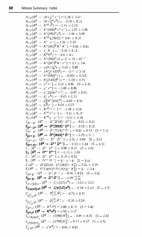
88888888 Meson Summary TableACP (B0 → (Kπ)∗+0 π−) = 0.09 ± 0.07ACP (B0 → (Kπ)∗00 π0) = −0.15 ± 0.11ACP (B0 → K∗0π0) = −0.15 ± 0.13ACP (B0 → K∗(892)0π+π−) = 0.07 ± 0.05ACP (B0 → K∗(892)0 ρ0) = −0.06 ± 0.09ACP (B0 → K∗0 f0(980)) = 0.07 ± 0.10ACP (B0 → K∗+ρ−) = 0.21 ± 0.15ACP (B0 → K∗(892)0K+K−) = 0.01 ± 0.05ACP (B0 → a−1 K+) = −0.16 ± 0.12ACP (B0 → K0K0) = −0.6 ± 0.7ACP (B0 → K∗(892)0φ) = (0 ± 4)× 10−2ACP (B0 → K∗(892)0K−π+) = 0.2 ± 0.4ACP (B0 → φ(K π)∗00 ) = 0.12 ± 0.08ACP (B0 → φK∗2(1430)0) = −0.11 ± 0.10ACP (B0 → K∗(892)0 γ) = −0.002 ± 0.015ACP (B0 → K∗2(1430)0 γ) = −0.08 ± 0.15ACP (B0 → ρ+π−) = 0.13 ± 0.06 (S = 1.1)ACP (B0 → ρ−π+) = −0.08 ± 0.08ACP (B0 → a1(1260)±π∓) = −0.07 ± 0.06ACP (B0 → b−1 π+) = −0.05 ± 0.10ACP (B0 → ppK∗(892)0) = 0.05 ± 0.12ACP (B0 → pπ−) = 0.04 ± 0.07ACP (B0 → K∗0 ℓ+ ℓ−) = −0.05 ± 0.10ACP (B0 → K∗0 e+ e−) = −0.21 ± 0.19ACP (B0 → K∗0µ+µ−) = −0.07 ± 0.04CD∗−D+ (B0 → D∗(2010)−D+) = −0.01 ± 0.11SD∗−D+ (B0 → D∗(2010)−D+)SD∗−D+ (B0 → D∗(2010)−D+)SD∗−D+ (B0 → D∗(2010)−D+)SD∗−D+ (B0 → D∗(2010)−D+) = −0.72 ± 0.15CD∗+D− (B0 → D∗(2010)+D−) = 0.00 ± 0.13 (S = 1.3)SD∗+D− (B0 → D∗(2010)+D−)SD∗+D− (B0 → D∗(2010)+D−)SD∗+D− (B0 → D∗(2010)+D−)SD∗+D− (B0 → D∗(2010)+D−) = −0.73 ± 0.14CD∗+D∗− (B0 → D∗+D∗−) = 0.01 ± 0.09 (S = 1.6)SD∗+D∗− (B0 → D∗+D∗−)SD∗+D∗− (B0 → D∗+D∗−)SD∗+D∗− (B0 → D∗+D∗−)SD∗+D∗− (B0 → D∗+D∗−) = −0.59 ± 0.14 (S = 1.8)C+ (B0 → D∗+D∗−) = 0.00 ± 0.10 (S = 1.6)S+ (B0 → D∗+D∗−)S+ (B0 → D∗+D∗−)S+ (B0 → D∗+D∗−)S+ (B0 → D∗+D∗−) = −0.73 ± 0.09C− (B0 → D∗+D∗−) = 0.19 ± 0.31S− (B0 → D∗+D∗−) = 0.1 ± 1.6 (S = 3.5)C (B0 → D∗(2010)+D∗(2010)−K0S) = 0.01 ± 0.29S (B0 → D∗(2010)+D∗(2010)−K0S) = 0.1 ± 0.4CD+D− (B0 → D+D−) = −0.46 ± 0.21 (S = 1.8)SD+D− (B0 → D+D−)SD+D− (B0 → D+D−)SD+D− (B0 → D+D−)SD+D− (B0 → D+D−) = −0.99+0.17−0.14CJ/ψ(1S)π0 (B0 → J/ψ(1S)π0) = −0.13 ± 0.13SJ/ψ(1S)π0 (B0 → J/ψ(1S)π0)SJ/ψ(1S)π0 (B0 → J/ψ(1S)π0)SJ/ψ(1S)π0 (B0 → J/ψ(1S)π0)SJ/ψ(1S)π0 (B0 → J/ψ(1S)π0) = −0.94 ± 0.29 (S = 1.9)CD(∗)
CPh0 (B0 → D(∗)
CP h0) = −0.23 ± 0.16SD(∗)CP
h0 (B0 → D(∗)CP h0) = −0.56 ± 0.24CK0π0 (B0 → K0π0) = 0.00 ± 0.13 (S = 1.4)SK0π0 (B0 → K0π0)SK0π0 (B0 → K0π0)SK0π0 (B0 → K0π0)SK0π0 (B0 → K0π0) = 0.58 ± 0.17C
η′(958)K0S (B0 → η′(958)K0S ) = −0.04 ± 0.20 (S = 2.5)Sη′(958)K0S (B0 → η′(958)K0S) = 0.43 ± 0.17 (S = 1.5)Cη′K0 (B0 → η′K0) = −0.05 ± 0.05
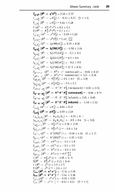
Meson Summary Table 89898989Sη′K0 (B0 → η′K0)Sη′K0 (B0 → η′K0)Sη′K0 (B0 → η′K0)Sη′K0 (B0 → η′K0) = 0.60 ± 0.07CωK0S (B0 → ωK0S ) = −0.30 ± 0.28 (S = 1.6)SωK0S (B0 → ωK0S ) = 0.43 ± 0.24C (B0 → K0S π0π0) = 0.2 ± 0.5S (B0 → K0S π0π0) = 0.7 ± 0.7Cρ0K0S (B0 → ρ0K0S ) = −0.04 ± 0.20Sρ0K0S (B0 → ρ0K0S ) = 0.50+0.17
−0.21Cf0K0S (B0 → f0(980)K0S ) = 0.29 ± 0.20Sf0K0S (B0 → f0(980)K0S )Sf0K0S (B0 → f0(980)K0S )Sf0K0S (B0 → f0(980)K0S )Sf0K0S (B0 → f0(980)K0S ) = −0.50 ± 0.16Sf2K0S (B0 → f2(1270)K0S ) = −0.5 ± 0.5Cf2K0S (B0 → f2(1270)K0S ) = 0.3 ± 0.4Sfx K0S (B0 → fx (1300)K0S ) = −0.2 ± 0.5Cfx K0S (B0 → fx (1300)K0S ) = 0.13 ± 0.35SK0π+π− (B0 → K0π+π− nonresonant) = −0.01 ± 0.33CK0π+π− (B0 → K0π+π− nonresonant) = 0.01 ± 0.26CK0S K0S (B0 → K0S K0S) = 0.0 ± 0.4 (S = 1.4)SK0S K0S (B0 → K0S K0S ) = −0.8 ± 0.5CK+K−K0S (B0 → K+K−K0S nonresonant) = 0.06 ± 0.08SK+K−K0S (B0 → K+K−K0S nonresonant)SK+K−K0S (B0 → K+K−K0S nonresonant)SK+K−K0S (B0 → K+K−K0S nonresonant)SK+K−K0S (B0 → K+K−K0S nonresonant) = −0.66 ± 0.11CK+K−K0S (B0 → K+K−K0S in lusive) = 0.01 ± 0.09SK+K−K0S (B0 → K+K−K0S in lusive)SK+K−K0S (B0 → K+K−K0S in lusive)SK+K−K0S (B0 → K+K−K0S in lusive)SK+K−K0S (B0 → K+K−K0S in lusive) = −0.65 ± 0.12CφK0S (B0 → φK0S ) = 0.01 ± 0.14SφK0S (B0 → φK0S )SφK0S (B0 → φK0S )SφK0S (B0 → φK0S )SφK0S (B0 → φK0S ) = 0.59 ± 0.14CKS KS KS (B0 → KS KS KS ) = −0.23 ± 0.14SKS KS KS (B0 → KS KS KS ) = −0.5 ± 0.6 (S = 3.0)CK0S π0 γ
(B0 → K0S π0 γ) = 0.36 ± 0.33SK0S π0 γ(B0 → K0S π0 γ) = −0.8 ± 0.6CK∗0 γ (B0 → K∗(892)0γ) = −0.04 ± 0.16 (S = 1.2)SK∗0 γ (B0 → K∗(892)0γ) = −0.15 ± 0.22CηK0 γ (B0 → ηK0 γ) = −0.3 ± 0.4SηK0 γ (B0 → ηK0 γ) = −0.2 ± 0.5CK0φγ (B0 → K0φγ) = −0.3 ± 0.6SK0φγ (B0 → K0φγ) = 0.7+0.7
−1.1C(B0 → K0S ρ0γ) = −0.05 ± 0.19S(B0 → K0S ρ0 γ) = 0.11 ± 0.34C (B0 → ρ0 γ) = 0.4 ± 0.5S (B0 → ρ0 γ) = −0.8 ± 0.7Cππ (B0 → π+π−)Cππ (B0 → π+π−)Cππ (B0 → π+π−)Cππ (B0 → π+π−) = −0.31 ± 0.05Sππ (B0 → π+π−)Sππ (B0 → π+π−)Sππ (B0 → π+π−)Sππ (B0 → π+π−) = −0.67 ± 0.06Cπ0π0(B0 → π0π0) = −0.43 ± 0.24Cρπ (B0 → ρ+π−) = −0.03 ± 0.07 (S = 1.2)
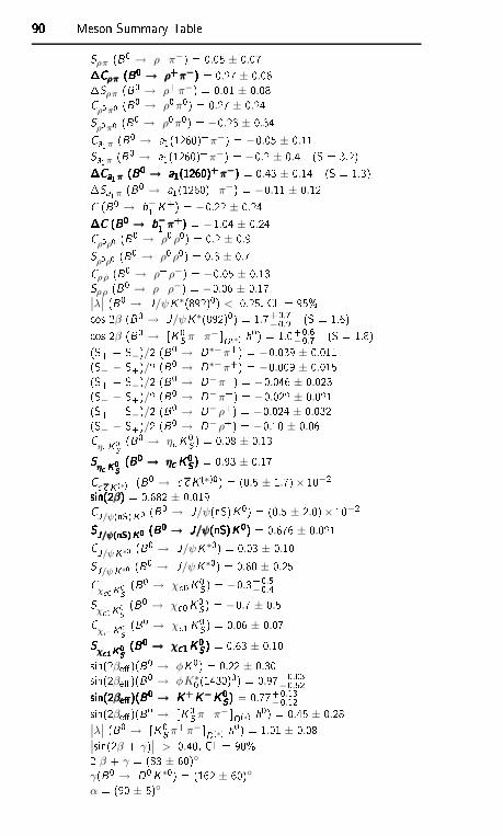
90909090 Meson Summary TableSρπ (B0 → ρ+π−) = 0.05 ± 0.07Cρπ (B0 → ρ+π−)Cρπ (B0 → ρ+π−)Cρπ (B0 → ρ+π−)Cρπ (B0 → ρ+π−) = 0.27 ± 0.06Sρπ (B0 → ρ+π−) = 0.01 ± 0.08Cρ0 π0 (B0 → ρ0π0) = 0.27 ± 0.24Sρ0 π0 (B0 → ρ0π0) = −0.23 ± 0.34Ca1 π (B0 → a1(1260)+π−) = −0.05 ± 0.11Sa1 π (B0 → a1(1260)+π−) = −0.2 ± 0.4 (S = 3.2)Ca1 π (B0 → a1(1260)+π−)Ca1 π (B0 → a1(1260)+π−)Ca1 π (B0 → a1(1260)+π−)Ca1 π (B0 → a1(1260)+π−) = 0.43 ± 0.14 (S = 1.3)Sa1 π (B0 → a1(1260)+π−) = −0.11 ± 0.12C (B0 → b−1 K+) = −0.22 ± 0.24C (B0 → b−1 π+)C (B0 → b−1 π+)C (B0 → b−1 π+)C (B0 → b−1 π+) = −1.04 ± 0.24Cρ0ρ0 (B0 → ρ0 ρ0) = 0.2 ± 0.9Sρ0ρ0 (B0 → ρ0 ρ0) = 0.3 ± 0.7Cρρ (B0 → ρ+ρ−) = −0.05 ± 0.13Sρρ (B0 → ρ+ρ−) = −0.06 ± 0.17∣
∣λ∣
∣ (B0 → J/ψK∗(892)0) < 0.25, CL = 95% os 2β (B0 → J/ψK∗(892)0) = 1.7+0.7−0.9 (S = 1.6) os 2β (B0 → [K0S π+π− D(∗) h0) = 1.0+0.6
−0.7 (S = 1.8)(S+ + S−)/2 (B0 → D∗−π+) = −0.039 ± 0.011(S− − S+)/2 (B0 → D∗−π+) = −0.009 ± 0.015(S+ + S−)/2 (B0 → D−π+) = −0.046 ± 0.023(S− − S+)/2 (B0 → D−π+) = −0.022 ± 0.021(S+ + S−)/2 (B0 → D− ρ+) = −0.024 ± 0.032(S− − S+)/2 (B0 → D− ρ+) = −0.10 ± 0.06Cη K0S (B0 → η K0S ) = 0.08 ± 0.13Sη K0S (B0 → η K0S )Sη K0S (B0 → η K0S )Sη K0S (B0 → η K0S )Sη K0S (B0 → η K0S ) = 0.93 ± 0.17C K (∗)0 (B0 → K (∗)0) = (0.5 ± 1.7)× 10−2sin(2β)sin(2β)sin(2β)sin(2β) = 0.682 ± 0.019CJ/ψ(nS)K0 (B0 → J/ψ(nS)K0) = (0.5 ± 2.0)× 10−2SJ/ψ(nS)K0 (B0 → J/ψ(nS)K0)SJ/ψ(nS)K0 (B0 → J/ψ(nS)K0)SJ/ψ(nS)K0 (B0 → J/ψ(nS)K0)SJ/ψ(nS)K0 (B0 → J/ψ(nS)K0) = 0.676 ± 0.021CJ/ψK∗0 (B0 → J/ψK∗0) = 0.03 ± 0.10SJ/ψK∗0 (B0 → J/ψK∗0) = 0.60 ± 0.25Cχ 0K0S (B0 → χ 0K0S ) = −0.3+0.5
−0.4Sχ 0K0S (B0 → χ 0K0S ) = −0.7 ± 0.5Cχ 1K0S (B0 → χ 1K0S ) = 0.06 ± 0.07Sχ 1K0S (B0 → χ 1K0S )Sχ 1K0S (B0 → χ 1K0S )Sχ 1K0S (B0 → χ 1K0S )Sχ 1K0S (B0 → χ 1K0S ) = 0.63 ± 0.10sin(2βe)(B0 → φK0) = 0.22 ± 0.30sin(2βe)(B0 → φK∗0 (1430)0) = 0.97+0.03
−0.52sin(2βe)(B0 → K+K−K0S)sin(2βe)(B0 → K+K−K0S)sin(2βe)(B0 → K+K−K0S)sin(2βe)(B0 → K+K−K0S) = 0.77+0.13−0.12sin(2βe)(B0 → [K0S π+π− D(∗) h0) = 0.45 ± 0.28
∣
∣λ∣
∣ (B0 → [K0S π+π− D(∗) h0) = 1.01 ± 0.08∣
∣sin(2β + γ)∣∣ > 0.40, CL = 90%2 β + γ = (83 ± 60)γ(B0 → D0K∗0) = (162 ± 60)α = (90 ± 5)
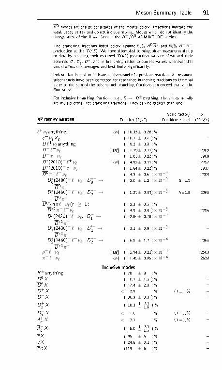
Meson Summary Table 91919191B0 modes are harge onjugates of the modes below. Rea tions indi ate theweak de ay vertex and do not in lude mixing. Modes whi h do not identify the harge state of the B are listed in the B±/B0 ADMIXTURE se tion.The bran hing fra tions listed below assume 50% B0B0 and 50% B+B−produ tion at the (4S). We have attempted to bring older measurements upto date by res aling their assumed (4S) produ tion ratio to 50:50 and theirassumed D, Ds , D∗, and ψ bran hing ratios to urrent values whenever thiswould ae t our averages and best limits signi antly.Indentation is used to indi ate a sub hannel of a previous rea tion. All resonantsub hannels have been orre ted for resonan e bran hing fra tions to the nalstate so the sum of the sub hannel bran hing fra tions an ex eed that of thenal state.For in lusive bran hing fra tions, e.g., B → D± anything, the values usuallyare multipli ities, not bran hing fra tions. They an be greater than one.S ale fa tor/ pB0 DECAY MODESB0 DECAY MODESB0 DECAY MODESB0 DECAY MODES Fra tion (i /) Conden e level (MeV/ )ℓ+νℓ anything [sss ( 10.33± 0.28) % e+ νe X ( 10.1 ± 0.4 ) % D ℓ+νℓ anything ( 9.2 ± 0.8 ) % D− ℓ+νℓ [sss ( 2.19± 0.12) % 2309D− τ+ ντ ( 1.03± 0.22) % 1909D∗(2010)− ℓ+νℓ [sss ( 4.93± 0.11) % 2257D∗(2010)− τ+ ντ ( 1.84± 0.22) % 1837D0π− ℓ+νℓ ( 4.3 ± 0.6 )× 10−3 2308D∗0(2400)− ℓ+νℓ, D∗−0 →D0π−
( 3.0 ± 1.2 )× 10−3 S=1.8 D∗2(2460)− ℓ+νℓ, D∗−2 →D0π−( 1.21± 0.33)× 10−3 S=1.8 2065D(∗) nπℓ+ νℓ (n ≥ 1) ( 2.3 ± 0.5 ) % D∗0π− ℓ+νℓ ( 4.9 ± 0.8 )× 10−3 2256D1(2420)− ℓ+νℓ, D−1 →D∗0π−( 2.80± 0.28)× 10−3 D ′1(2430)− ℓ+νℓ, D ′−1 →D∗0π−( 3.1 ± 0.9 )× 10−3 D∗2(2460)− ℓ+νℓ, D∗−2 →D∗0π−( 6.8 ± 1.2 )× 10−4 2065
ρ− ℓ+νℓ [sss ( 2.94± 0.21)× 10−4 2583π− ℓ+νℓ [sss ( 1.45± 0.05)× 10−4 2638In lusive modesIn lusive modesIn lusive modesIn lusive modesK± anything ( 78 ± 8 ) % D0X ( 8.1 ± 1.5 ) % D0X ( 47.4 ± 2.8 ) % D+X < 3.9 % CL=90% D−X ( 36.9 ± 3.3 ) % D+s X ( 10.3 + 2.1
− 1.8 ) % D−s X < 2.6 % CL=90% + X < 3.1 % CL=90% − X ( 5.0 + 2.1− 1.5 ) % X ( 95 ± 5 ) % X ( 24.6 ± 3.1 ) % X (119 ± 6 ) %
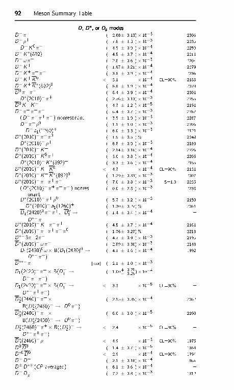
92929292 Meson Summary TableD, D∗, or Ds modesD, D∗, or Ds modesD, D∗, or Ds modesD, D∗, or Ds modesD−π+ ( 2.68± 0.13)× 10−3 2306D− ρ+ ( 7.8 ± 1.3 )× 10−3 2235D−K0π+ ( 4.9 ± 0.9 )× 10−4 2259D−K∗(892)+ ( 4.5 ± 0.7 )× 10−4 2211D−ωπ+ ( 2.8 ± 0.6 )× 10−3 2204D−K+ ( 1.97± 0.21)× 10−4 2279D−K+π+π− ( 3.8 ± 0.9 )× 10−4 2236D−K+K0 < 3.1 × 10⁻⁴ CL=90% 2188D−K+K∗(892)0 ( 8.8 ± 1.9 )× 10−4 2070D0π+π− ( 8.4 ± 0.9 )× 10−4 2301D∗(2010)−π+ ( 2.76± 0.13)× 10−3 2255D0K+K− ( 4.7 ± 1.2 )× 10−5 2191D−π+π+π− ( 6.4 ± 0.7 )× 10−3 2287(D−π+π+π− ) nonresonant ( 3.9 ± 1.9 )× 10−3 2287D−π+ρ0 ( 1.1 ± 1.0 )× 10−3 2206D− a1(1260)+ ( 6.0 ± 3.3 )× 10−3 2121D∗(2010)−π+π0 ( 1.5 ± 0.5 ) % 2248D∗(2010)− ρ+ ( 6.8 ± 0.9 )× 10−3 2180D∗(2010)−K+ ( 2.14± 0.16)× 10−4 2226D∗(2010)−K0π+ ( 3.0 ± 0.8 )× 10−4 2205D∗(2010)−K∗(892)+ ( 3.3 ± 0.6 )× 10−4 2155D∗(2010)−K+K0 < 4.7 × 10⁻⁴ CL=90% 2131D∗(2010)−K+K∗(892)0 ( 1.29± 0.33)× 10−3 2007D∗(2010)−π+π+π− ( 7.0 ± 0.8 )× 10−3 S=1.3 2235(D∗(2010)−π+π+π− ) nonres-onant ( 0.0 ± 2.5 )× 10−3 2235D∗(2010)−π+ρ0 ( 5.7 ± 3.2 )× 10−3 2150D∗(2010)− a1(1260)+ ( 1.30± 0.27) % 2061D1(2420)0π−π+, D01 →D∗−π+ ( 1.4 ± 0.4 )× 10−4 D∗(2010)−K+π−π+ ( 4.5 ± 0.7 )× 10−4 2181D∗(2010)−π+π+π−π0 ( 1.76± 0.27) % 2218D∗− 3π+2π− ( 4.7 ± 0.9 )× 10−3 2195D∗(2010)−ωπ+ ( 2.89± 0.30)× 10−3 2148D1(2430)0ω× B(D1(2430)0 →D∗−π+) ( 4.1 ± 1.6 )× 10−4 1992D∗∗−π+ [xxx ( 2.1 ± 1.0 )× 10−3 D1(2420)−π+× B(D−1 →D−π+π−) ( 1.00+ 0.21− 0.25)× 10−4 D1(2420)−π+× B(D−1 →D∗−π+π−) < 3.3 × 10⁻⁵ CL=90% D∗2(2460)−π+×B(D∗2(2460)− → D0π−) ( 2.15± 0.35)× 10−4 2062D∗0(2400)−π+×B(D∗0(2400)− → D0π−) ( 6.0 ± 3.0 )× 10−5 2090
D∗2(2460)−π+× B((D∗2)− →D∗−π+π−) < 2.4 × 10⁻⁵ CL=90% D∗2(2460)− ρ+ < 4.9 × 10⁻³ CL=90% 1975D0D0 ( 1.4 ± 0.7 )× 10−5 1868D∗0D0 < 2.9 × 10⁻⁴ CL=90% 1794D−D+ ( 2.11± 0.18)× 10−4 1864D±D∗∓ (CP-averaged) ( 6.1 ± 0.6 )× 10−4 D−D+s ( 7.2 ± 0.8 )× 10−3 1812
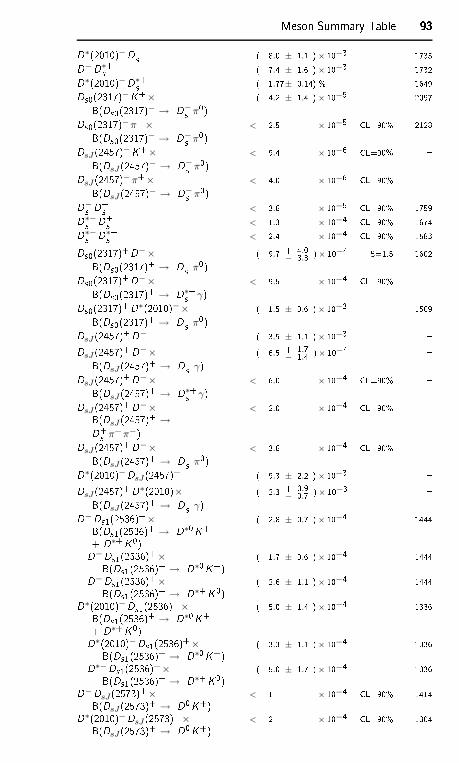
Meson Summary Table 93939393D∗(2010)−D+s ( 8.0 ± 1.1 )× 10−3 1735D−D∗+s ( 7.4 ± 1.6 )× 10−3 1732D∗(2010)−D∗+s ( 1.77± 0.14) % 1649Ds0(2317)−K+×B(Ds0(2317)− → D−s π0) ( 4.2 ± 1.4 )× 10−5 2097Ds0(2317)−π+×B(Ds0(2317)− → D−s π0) < 2.5 × 10⁻⁵ CL=90% 2128DsJ (2457)−K+×B(DsJ (2457)− → D−s π0) < 9.4 × 10⁻⁶ CL=90% DsJ (2457)−π+×B(DsJ (2457)− → D−s π0) < 4.0 × 10⁻⁶ CL=90% D−s D+s < 3.6 × 10⁻⁵ CL=90% 1759D∗−s D+s < 1.3 × 10⁻⁴ CL=90% 1674D∗−s D∗+s < 2.4 × 10⁻⁴ CL=90% 1583Ds0(2317)+D−×B(Ds0(2317)+ → D+s π0) ( 9.7 + 4.0− 3.3 )× 10−4 S=1.5 1602Ds0(2317)+D−×B(Ds0(2317)+ → D∗+s γ) < 9.5 × 10⁻⁴ CL=90% Ds0(2317)+D∗(2010)−×B(Ds0(2317)+ → D+s π0) ( 1.5 ± 0.6 )× 10−3 1509DsJ (2457)+D− ( 3.5 ± 1.1 )× 10−3 DsJ (2457)+D−×B(DsJ (2457)+ → D+s γ) ( 6.5 + 1.7− 1.4 )× 10−4 DsJ (2457)+D−×B(DsJ (2457)+ → D∗+s γ) < 6.0 × 10⁻⁴ CL=90% DsJ (2457)+D−×B(DsJ (2457)+ →D+s π+π−) < 2.0 × 10⁻⁴ CL=90% DsJ (2457)+D−×B(DsJ (2457)+ → D+s π0) < 3.6 × 10⁻⁴ CL=90% D∗(2010)−DsJ(2457)+ ( 9.3 ± 2.2 )× 10−3 DsJ (2457)+D∗(2010)×B(DsJ (2457)+ → D+s γ) ( 2.3 + 0.9− 0.7 )× 10−3 D−Ds1(2536)+×B(Ds1(2536)+ → D∗0K++ D∗+K0) ( 2.8 ± 0.7 )× 10−4 1444D−Ds1(2536)+×B(Ds1(2536)+ → D∗0K+) ( 1.7 ± 0.6 )× 10−4 1444D−Ds1(2536)+×B(Ds1(2536)+ → D∗+K0) ( 2.6 ± 1.1 )× 10−4 1444D∗(2010)−Ds1(2536)+×B(Ds1(2536)+ → D∗0K++ D∗+K0) ( 5.0 ± 1.4 )× 10−4 1336D∗(2010)−Ds1(2536)+×B(Ds1(2536)+ → D∗0K+) ( 3.3 ± 1.1 )× 10−4 1336D∗−Ds1(2536)+×B(Ds1(2536)+ → D∗+K0) ( 5.0 ± 1.7 )× 10−4 1336D−DsJ(2573)+×B(DsJ (2573)+ → D0K+) < 1 × 10⁻⁴ CL=90% 1414D∗(2010)−DsJ(2573)+×B(DsJ (2573)+ → D0K+) < 2 × 10⁻⁴ CL=90% 1304
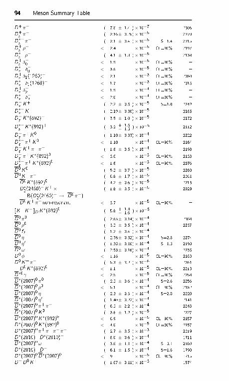
94949494 Meson Summary TableD+π− ( 7.8 ± 1.4 )× 10−7 2306D+s π− ( 2.16± 0.26)× 10−5 2270D∗+s π− ( 2.1 ± 0.4 )× 10−5 S=1.4 2215D+s ρ− < 2.4 × 10⁻⁵ CL=90% 2197D∗+s ρ− ( 4.1 ± 1.3 )× 10−5 2138D+s a−0 < 1.9 × 10⁻⁵ CL=90% D∗+s a−0 < 3.6 × 10⁻⁵ CL=90% D+s a1(1260)− < 2.1 × 10⁻³ CL=90% 2080D∗+s a1(1260)− < 1.7 × 10⁻³ CL=90% 2015D+s a−2 < 1.9 × 10⁻⁴ CL=90% D∗+s a−2 < 2.0 × 10⁻⁴ CL=90% D−s K+ ( 2.2 ± 0.5 )× 10−5 S=1.8 2242D∗−s K+ ( 2.19± 0.30)× 10−5 2185D−s K∗(892)+ ( 3.5 ± 1.0 )× 10−5 2172D∗−s K∗(892)+ ( 3.2 + 1.5− 1.3 )× 10−5 2112D−s π+K0 ( 1.10± 0.33)× 10−4 2222D∗−s π+K0 < 1.10 × 10⁻⁴ CL=90% 2164D−s K+π+π− ( 1.8 ± 0.5 )× 10−4 2198D−s π+K∗(892)0 < 3.0 × 10⁻³ CL=90% 2138D∗−s π+K∗(892)0 < 1.6 × 10⁻³ CL=90% 2076D0K0 ( 5.2 ± 0.7 )× 10−5 2280D0K+π− ( 8.8 ± 1.7 )× 10−5 2261D0K∗(892)0 ( 4.2 ± 0.6 )× 10−5 2213D∗2(2460)−K+×B(D∗2(2460)− → D0π−) ( 1.8 ± 0.5 )× 10−5 2029D0K+π− non-resonant < 3.7 × 10⁻⁵ CL=90% [K+K− DK∗(892)0 ( 5.8 + 1.8− 1.6 )× 10−5 D0π0 ( 2.63± 0.14)× 10−4 2308D0 ρ0 ( 3.2 ± 0.5 )× 10−4 2237D0 f2 ( 1.2 ± 0.4 )× 10−4 D0 η ( 2.36± 0.32)× 10−4 S=2.5 2274D0 η′ ( 1.38± 0.16)× 10−4 S=1.3 2198D0ω ( 2.53± 0.16)× 10−4 2235D0φ < 1.16 × 10⁻⁵ CL=90% 2183D0K+π− ( 5.3 ± 3.2 )× 10−6 2261D0K∗(892)0 < 1.1 × 10⁻⁵ CL=90% 2213D∗0γ < 2.5 × 10⁻⁵ CL=90% 2258D∗(2007)0π0 ( 2.2 ± 0.6 )× 10−4 S=2.6 2256D∗(2007)0 ρ0 < 5.1 × 10⁻⁴ CL=90% 2182D∗(2007)0 η ( 2.3 ± 0.6 )× 10−4 S=2.8 2220D∗(2007)0 η′ ( 1.40± 0.22)× 10−4 2141D∗(2007)0π+π− ( 6.2 ± 2.2 )× 10−4 2248D∗(2007)0K0 ( 3.6 ± 1.2 )× 10−5 2227D∗(2007)0K∗(892)0 < 6.9 × 10⁻⁵ CL=90% 2157D∗(2007)0K∗(892)0 < 4.0 × 10⁻⁵ CL=90% 2157D∗(2007)0π+π+π−π− ( 2.7 ± 0.5 )× 10−3 2219D∗(2010)+D∗(2010)− ( 8.0 ± 0.6 )× 10−4 1711D∗(2007)0ω ( 3.6 ± 1.1 )× 10−4 S=3.1 2180D∗(2010)+D− ( 6.1 ± 1.5 )× 10−4 S=1.6 1790D∗(2007)0D∗(2007)0 < 9 × 10⁻⁵ CL=90% 1715D−D0K+ ( 1.07± 0.11)× 10−3 1574
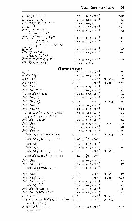
Meson Summary Table 95959595D−D∗(2007)0K+ ( 3.5 ± 0.4 )× 10−3 1478D∗(2010)−D0K+ ( 2.47± 0.21)× 10−3 1479D∗(2010)−D∗(2007)0K+ ( 1.06± 0.09) % 1366D−D+K0 ( 7.5 ± 1.7 )× 10−4 1568D∗(2010)−D+K0 +D−D∗(2010)+K0 ( 6.4 ± 0.5 )× 10−3 1473D∗(2010)−D∗(2010)+K0 ( 8.1 ± 0.7 )× 10−3 1360D∗−Ds1(2536)+×B(Ds1(2536)+ → D∗+K0) ( 8.0 ± 2.4 )× 10−4 1336D0D0K0 ( 2.7 ± 1.1 )× 10−4 1574D0D∗(2007)0K0 +D∗(2007)0D0K0 ( 1.1 ± 0.5 )× 10−3 1478D∗(2007)0D∗(2007)0K0 ( 2.4 ± 0.9 )× 10−3 1365(D+D∗ )(D+D∗ )K ( 3.68± 0.26) % Charmonium modesCharmonium modesCharmonium modesCharmonium modesη K0 ( 7.9 ± 1.2 )× 10−4 1751η K∗(892)0 ( 6.3 ± 0.9 )× 10−4 1646η (2S)K∗0 < 3.9 × 10⁻⁴ CL=90% 1157h (1P)K∗0 < 4 × 10⁻⁴ CL=90% 1253J/ψ(1S)K0 ( 8.73± 0.32)× 10−4 1683J/ψ(1S)K+π− ( 1.2 ± 0.6 )× 10−3 1652J/ψ(1S)K∗(892)0 ( 1.32± 0.06)× 10−3 1571J/ψ(1S)ηK0S ( 8 ± 4 )× 10−5 1508J/ψ(1S)η′K0S < 2.5 × 10⁻⁵ CL=90% 1271J/ψ(1S)φK0 ( 9.4 ± 2.6 )× 10−5 1224J/ψ(1S)ωK0 ( 2.3 ± 0.4 )× 10−4 1386X (3872)K0× B(X → J/ψω) ( 6.0 ± 3.2 )× 10−6 1140
χ 0(2P), χ 0 → J/ψω ( 2.1 ± 0.9 )× 10−5 1102J/ψ(1S)K (1270)0 ( 1.3 ± 0.5 )× 10−3 1390J/ψ(1S)π0 ( 1.76± 0.16)× 10−5 S=1.1 1728J/ψ(1S)η ( 1.23± 0.19)× 10−5 1672J/ψ(1S)π+π− ( 4.03± 0.18)× 10−5 1716J/ψ(1S)π+π− nonresonant < 1.2 × 10⁻⁵ CL=90% 1716J/ψ(1S) f0(500), f0 → ππ ( 6.5 + 2.6− 1.1 )× 10−6 J/ψ(1S) f2 ( 4.2 ± 0.7 )× 10−6 J/ψ(1S)ρ0 ( 2.58± 0.21)× 10−5 1612J/ψ(1S) f0(980), f0 → π+π− < 1.1 × 10⁻⁶ CL=90% J/ψ(1S)ρ(1450)0, ρ0 → ππ ( 2.1 + 2.5− 0.7 )× 10−6 J/ψ(1S)ω ( 2.3 ± 0.6 )× 10−5 1609J/ψ(1S)K+K− ( 2.6 ± 0.4 )× 10−6 1533J/ψ(1S)a0(980), a0 →K+K−
( 4.7 ± 3.4 )× 10−7 J/ψ(1S)φ < 1.9 × 10⁻⁷ CL=90% 1520J/ψ(1S)η′(958) < 7.4 × 10⁻⁶ CL=90% 1546J/ψ(1S)K0π+π− ( 1.0 ± 0.4 )× 10−3 1611J/ψ(1S)K0ρ0 ( 5.4 ± 3.0 )× 10−4 1390J/ψ(1S)K∗(892)+π− ( 8 ± 4 )× 10−4 1514J/ψ(1S)K∗(892)0π+π− ( 6.6 ± 2.2 )× 10−4 1447X (3872)−K+ < 5 × 10⁻⁴ CL=90% X (3872)−K+× B(X (3872)− →J/ψ(1S)π−π0) [yyy < 4.2 × 10⁻⁶ CL=90% X (3872)K0× B(X →J/ψπ+π−) ( 4.3 ± 1.3 )× 10−6 1140
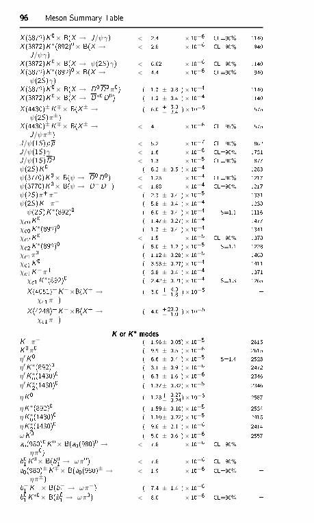
96969696 Meson Summary TableX (3872)K0× B(X → J/ψγ) < 2.4 × 10⁻⁶ CL=90% 1140X (3872)K∗(892)0× B(X →J/ψγ) < 2.8 × 10⁻⁶ CL=90% 940X (3872)K0× B(X → ψ(2S)γ) < 6.62 × 10⁻⁶ CL=90% 1140X (3872)K∗(892)0× B(X →ψ(2S)γ) < 4.4 × 10⁻⁶ CL=90% 940X (3872)K0× B(X → D0D0π0) ( 1.7 ± 0.8 )× 10−4 1140X (3872)K0× B(X → D∗0D0) ( 1.2 ± 0.4 )× 10−4 1140X (4430)±K∓× B(X± →ψ(2S)π±) ( 6.0 + 3.0
− 2.4 )× 10−5 575X (4430)±K∓× B(X± →J/ψπ±) < 4 × 10⁻⁶ CL=95% 575J/ψ(1S)pp < 5.2 × 10⁻⁷ CL=90% 862J/ψ(1S)γ < 1.6 × 10⁻⁶ CL=90% 1731J/ψ(1S)D0 < 1.3 × 10⁻⁵ CL=90% 877ψ(2S)K0 ( 6.2 ± 0.5 )× 10−4 1283ψ(3770)K0× B(ψ → D0D0) < 1.23 × 10⁻⁴ CL=90% 1217ψ(3770)K0× B(ψ → D−D+) < 1.88 × 10⁻⁴ CL=90% 1217ψ(2S)π+π− ( 2.3 ± 0.4 )× 10−5 1331ψ(2S)K+π− ( 5.8 ± 0.4 )× 10−4 1238
ψ(2S)K∗(892)0 ( 6.0 ± 0.4 )× 10−4 S=1.1 1116χ 0K0 ( 1.47± 0.27)× 10−4 1477χ 0K∗(892)0 ( 1.7 ± 0.4 )× 10−4 1341χ 2K0 < 1.5 × 10⁻⁵ CL=90% 1378χ 2K∗(892)0 ( 5.0 ± 1.2 )× 10−5 S=1.1 1228χ 1π0 ( 1.12± 0.28)× 10−5 1468χ 1K0 ( 3.93± 0.27)× 10−4 1411χ 1K−π+ ( 3.8 ± 0.4 )× 10−4 1371
χ 1K∗(892)0 ( 2.42± 0.21)× 10−4 S=1.3 1265X (4051)+K−×B(X+ →χ 1π+) ( 3.0 + 4.0
− 1.8 )× 10−5 X (4248)+K−×B(X+ →χ 1π+) ( 4.0 +20.0
− 1.0 )× 10−5 K or K∗ modesK or K∗ modesK or K∗ modesK or K∗ modesK+π− ( 1.96± 0.05)× 10−5 2615K0π0 ( 9.9 ± 0.5 )× 10−6 2615η′K0 ( 6.6 ± 0.4 )× 10−5 S=1.4 2528η′K∗(892)0 ( 3.1 ± 0.9 )× 10−6 2472η′K∗0(1430)0 ( 6.3 ± 1.6 )× 10−6 2346η′K∗2(1430)0 ( 1.37± 0.32)× 10−5 2346ηK0 ( 1.23+ 0.27
− 0.24)× 10−6 2587ηK∗(892)0 ( 1.59± 0.10)× 10−5 2534ηK∗0(1430)0 ( 1.10± 0.22)× 10−5 2415ηK∗2(1430)0 ( 9.6 ± 2.1 )× 10−6 2414ωK0 ( 5.0 ± 0.6 )× 10−6 2557a0(980)0K0× B(a0(980)0 →
ηπ0) < 7.8 × 10⁻⁶ CL=90% b01K0× B(b01 → ωπ0) < 7.8 × 10⁻⁶ CL=90% a0(980)±K∓× B(a0(980)± →ηπ±) < 1.9 × 10⁻⁶ CL=90% b−1 K+× B(b−1 → ωπ−) ( 7.4 ± 1.4 )× 10−6 b01K∗0× B(b01 → ωπ0) < 8.0 × 10⁻⁶ CL=90%
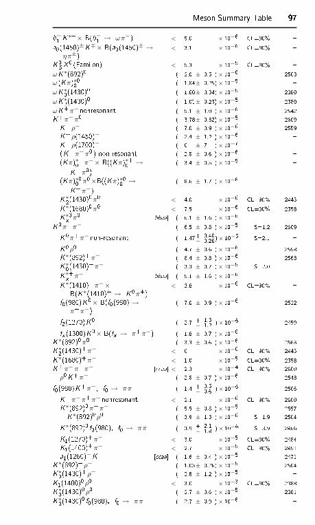
Meson Summary Table 97979797b−1 K∗+× B(b−1 → ωπ−) < 5.0 × 10⁻⁶ CL=90% a0(1450)±K∓× B(a0(1450)± →ηπ±) < 3.1 × 10⁻⁶ CL=90% K0S X 0 (Familon) < 5.3 × 10⁻⁵ CL=90%
ωK∗(892)0 ( 2.0 ± 0.5 )× 10−6 2503ω (Kπ)∗00 ( 1.84± 0.25)× 10−5 ωK∗0(1430)0 ( 1.60± 0.34)× 10−5 2380ωK∗2(1430)0 ( 1.01± 0.23)× 10−5 2380ωK+π− nonresonant ( 5.1 ± 1.0 )× 10−6 2542K+π−π0 ( 3.78± 0.32)× 10−5 2609K+ρ− ( 7.0 ± 0.9 )× 10−6 2559K+ρ(1450)− ( 2.4 ± 1.2 )× 10−6 K+ρ(1700)− ( 6 ± 7 )× 10−7 (K+π−π0 ) non-resonant ( 2.8 ± 0.6 )× 10−6 (Kπ)∗+0 π−× B((Kπ)∗+0 →K+π0) ( 3.4 ± 0.5 )× 10−5 (Kπ)∗00 π0×B((Kπ)∗00 →K+π−) ( 8.6 ± 1.7 )× 10−6 K∗2(1430)0π0 < 4.0 × 10⁻⁶ CL=90% 2445K∗(1680)0π0 < 7.5 × 10⁻⁶ CL=90% 2358K∗0x π0 [bbaa ( 6.1 ± 1.6 )× 10−6 K0π+π− ( 6.5 ± 0.8 )× 10−5 S=1.2 2609K0π+π− non-resonant ( 1.47+ 0.40
− 0.26)× 10−5 S=2.1 K0ρ0 ( 4.7 ± 0.6 )× 10−6 2558K∗(892)+π− ( 8.4 ± 0.8 )× 10−6 2563K∗0(1430)+π− ( 3.3 ± 0.7 )× 10−5 S=2.0 K∗+x π− [bbaa ( 5.1 ± 1.6 )× 10−6 K∗(1410)+π−×B(K∗(1410)+ → K0π+) < 3.8 × 10⁻⁶ CL=90% f0(980)K0× B(f0(980) →π+π−) ( 7.0 ± 0.9 )× 10−6 2522f2(1270)K0 ( 2.7 + 1.3
− 1.2 )× 10−6 2459fx (1300)K0× B(fx → π+π−) ( 1.8 ± 0.7 )× 10−6 K∗(892)0π0 ( 3.3 ± 0.6 )× 10−6 2563K∗2(1430)+π− < 6 × 10⁻⁶ CL=90% 2445K∗(1680)+π− < 1.0 × 10⁻⁵ CL=90% 2358K+π−π+π− [ aa < 2.3 × 10⁻⁴ CL=90% 2600ρ0K+π− ( 2.8 ± 0.7 )× 10−6 2543f0(980)K+π−, f0 → ππ ( 1.4 + 0.5
− 0.6 )× 10−6 2506K+π−π+π− nonresonant < 2.1 × 10⁻⁶ CL=90% 2600K∗(892)0π+π− ( 5.5 ± 0.5 )× 10−5 2557K∗(892)0 ρ0 ( 3.9 ± 1.3 )× 10−6 S=1.9 2504K∗(892)0 f0(980), f0 → ππ ( 3.9 + 2.1− 1.8 )× 10−6 S=3.9 2466K1(1270)+π− < 3.0 × 10⁻⁵ CL=90% 2484K1(1400)+π− < 2.7 × 10⁻⁵ CL=90% 2451a1(1260)−K+ [ aa ( 1.6 ± 0.4 )× 10−5 2471K∗(892)+ ρ− ( 1.03± 0.26)× 10−5 2504K∗0(1430)+ρ− ( 2.8 ± 1.2 )× 10−5 K1(1400)0 ρ0 < 3.0 × 10⁻³ CL=90% 2388K∗0(1430)0 ρ0 ( 2.7 ± 0.6 )× 10−5 2381K∗0(1430)0 f0(980), f0 → ππ ( 2.7 ± 0.9 )× 10−6
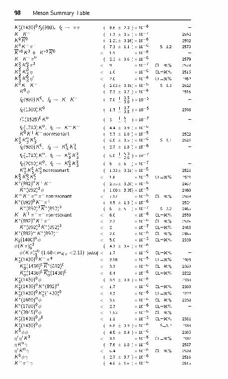
98989898 Meson Summary TableK∗2(1430)0 f0(980), f0 → ππ ( 8.6 ± 2.0 )× 10−6 K+K− ( 1.3 ± 0.5 )× 10−7 2593K0K0 ( 1.21± 0.16)× 10−6 2592K0K−π+ ( 7.3 ± 1.1 )× 10−6 S=1.2 2578K∗0K0 + K∗0K0 < 1.9 × 10⁻⁶ K+K−π0 ( 2.2 ± 0.6 )× 10−6 2579K0S K0S π0 < 9 × 10⁻⁷ CL=90% 2578K0S K0S η < 1.0 × 10⁻⁶ CL=90% 2515K0S K0S η′ < 2.0 × 10⁻⁶ CL=90% 2452K0K+K− ( 2.63± 0.15)× 10−5 S=1.3 2522K0φ ( 7.3 ± 0.7 )× 10−6 2516f0(980)K0, f0 → K+K− ( 7.0 + 3.5− 3.0 )× 10−6 f0(1500)K0 ( 1.3 + 0.7− 0.5 )× 10−5 2398f ′2(1525)0K0 ( 3 + 5− 4 )× 10−7 f0(1710)K0, f0 → K+K− ( 4.4 ± 0.9 )× 10−6 K0K+K−nonresonant ( 3.3 ± 1.0 )× 10−5 2522K0S K0S K0S ( 6.0 ± 0.5 )× 10−6 S=1.1 2521f0(980)K0, f0 → K0S K0S ( 2.7 ± 1.8 )× 10−6 f0(1710)K0, f0 → K0S K0S ( 5.0 + 5.0− 2.6 )× 10−7 f0(2010)K0, f0 → K0S K0S ( 5 ± 6 )× 10−7 K0S K0S K0S nonresonant ( 1.33± 0.31)× 10−5 2521K0S K0S K0L < 1.6 × 10⁻⁵ CL=90% 2521K∗(892)0K+K− ( 2.75± 0.26)× 10−5 2467K∗(892)0φ ( 1.00± 0.05)× 10−5 2460K+K−π+π−nonresonant < 7.17 × 10⁻⁵ CL=90% 2559K∗(892)0K−π+ ( 4.5 ± 1.3 )× 10−6 2524K∗(892)0K∗(892)0 ( 8 ± 5 )× 10−7 S=2.2 2485K+K+π−π−nonresonant < 6.0 × 10⁻⁶ CL=90% 2559K∗(892)0K+π− < 2.2 × 10⁻⁶ CL=90% 2524K∗(892)0K∗(892)0 < 2 × 10⁻⁷ CL=90% 2485K∗(892)+K∗(892)− < 2.0 × 10⁻⁶ CL=90% 2485K1(1400)0φ < 5.0 × 10⁻³ CL=90% 2339
φ(K π)∗00 ( 4.3 ± 0.4 )× 10−6 φ(K π)∗00 (1.60<mK π <2.15) [ddaa < 1.7 × 10⁻⁶ CL=90% K∗0(1430)0K−π+ < 3.18 × 10⁻⁵ CL=90% 2403K∗0(1430)0K∗(892)0 < 3.3 × 10⁻⁶ CL=90% 2360K∗0(1430)0K∗0(1430)0 < 8.4 × 10⁻⁶ CL=90% 2222K∗0(1430)0φ ( 3.9 ± 0.8 )× 10−6 2333K∗0(1430)0K∗(892)0 < 1.7 × 10⁻⁶ CL=90% 2360K∗0(1430)0K∗0(1430)0 < 4.7 × 10⁻⁶ CL=90% 2222K∗(1680)0φ < 3.5 × 10⁻⁶ CL=90% 2238K∗(1780)0φ < 2.7 × 10⁻⁶ CL=90% K∗(2045)0φ < 1.53 × 10⁻⁵ CL=90% K∗2(1430)0 ρ0 < 1.1 × 10⁻³ CL=90% 2381K∗2(1430)0φ ( 6.8 ± 0.9 )× 10−6 S=1.2 2333K0φφ ( 4.5 ± 0.9 )× 10−6 2305
η′ η′K0 < 3.1 × 10⁻⁵ CL=90% 2337ηK0 γ ( 7.6 ± 1.8 )× 10−6 2587η′K0γ < 6.4 × 10⁻⁶ CL=90% 2528K0φγ ( 2.7 ± 0.7 )× 10−6 2516K+π− γ ( 4.6 ± 1.4 )× 10−6 2615
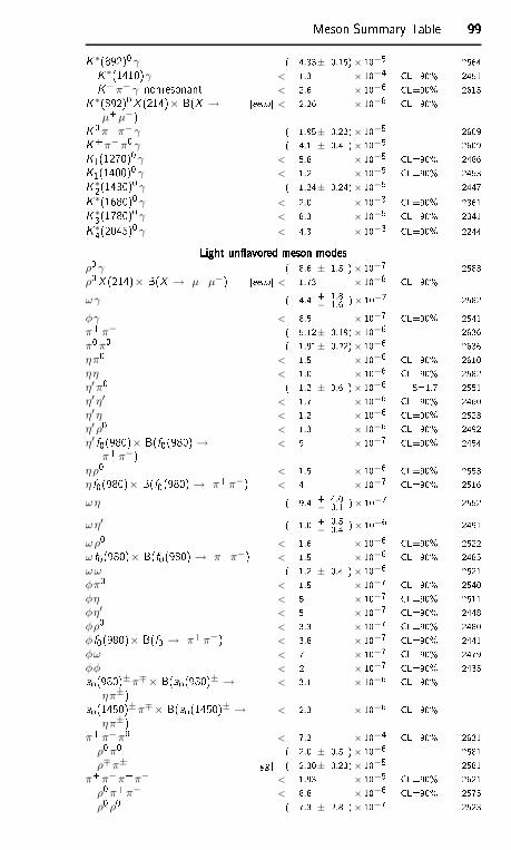
Meson Summary Table 99999999K∗(892)0 γ ( 4.33± 0.15)× 10−5 2564K∗(1410)γ < 1.3 × 10⁻⁴ CL=90% 2451K+π− γ nonresonant < 2.6 × 10⁻⁶ CL=90% 2615K∗(892)0X (214)× B(X →µ+µ−) [eeaa < 2.26 × 10⁻⁸ CL=90% K0π+π− γ ( 1.95± 0.22)× 10−5 2609K+π−π0 γ ( 4.1 ± 0.4 )× 10−5 2609K1(1270)0 γ < 5.8 × 10⁻⁵ CL=90% 2486K1(1400)0 γ < 1.2 × 10⁻⁵ CL=90% 2453K∗2(1430)0 γ ( 1.24± 0.24)× 10−5 2447K∗(1680)0 γ < 2.0 × 10⁻³ CL=90% 2361K∗3(1780)0 γ < 8.3 × 10⁻⁵ CL=90% 2341K∗4(2045)0 γ < 4.3 × 10⁻³ CL=90% 2244Light un avored meson modesLight un avored meson modesLight un avored meson modesLight un avored meson modes
ρ0 γ ( 8.6 ± 1.5 )× 10−7 2583ρ0X (214)× B(X → µ+µ−) [eeaa < 1.73 × 10⁻⁸ CL=90% ωγ ( 4.4 + 1.8
− 1.6 )× 10−7 2582φγ < 8.5 × 10⁻⁷ CL=90% 2541π+π− ( 5.12± 0.19)× 10−6 2636π0π0 ( 1.91± 0.22)× 10−6 2636ηπ0 < 1.5 × 10⁻⁶ CL=90% 2610ηη < 1.0 × 10⁻⁶ CL=90% 2582η′π0 ( 1.2 ± 0.6 )× 10−6 S=1.7 2551η′ η′ < 1.7 × 10⁻⁶ CL=90% 2460η′ η < 1.2 × 10⁻⁶ CL=90% 2523η′ρ0 < 1.3 × 10⁻⁶ CL=90% 2492η′ f0(980)× B(f0(980) →
π+π−) < 9 × 10⁻⁷ CL=90% 2454ηρ0 < 1.5 × 10⁻⁶ CL=90% 2553η f0(980)× B(f0(980) → π+π−) < 4 × 10⁻⁷ CL=90% 2516ωη ( 9.4 + 4.0
− 3.1 )× 10−7 2552ωη′ ( 1.0 + 0.5
− 0.4 )× 10−6 2491ωρ0 < 1.6 × 10⁻⁶ CL=90% 2522ω f0(980)× B(f0(980) → π+π−) < 1.5 × 10⁻⁶ CL=90% 2485ωω ( 1.2 ± 0.4 )× 10−6 2521φπ0 < 1.5 × 10⁻⁷ CL=90% 2540φη < 5 × 10⁻⁷ CL=90% 2511φη′ < 5 × 10⁻⁷ CL=90% 2448φρ0 < 3.3 × 10⁻⁷ CL=90% 2480φ f0(980)× B(f0 → π+π−) < 3.8 × 10⁻⁷ CL=90% 2441φω < 7 × 10⁻⁷ CL=90% 2479φφ < 2 × 10⁻⁷ CL=90% 2435a0(980)±π∓× B(a0(980)± →
ηπ±) < 3.1 × 10⁻⁶ CL=90% a0(1450)±π∓× B(a0(1450)± →ηπ±) < 2.3 × 10⁻⁶ CL=90%
π+π−π0 < 7.2 × 10⁻⁴ CL=90% 2631ρ0π0 ( 2.0 ± 0.5 )× 10−6 2581ρ∓π± [gg ( 2.30± 0.23)× 10−5 2581
π+π−π+π− < 1.93 × 10⁻⁵ CL=90% 2621ρ0π+π− < 8.8 × 10⁻⁶ CL=90% 2575ρ0 ρ0 ( 7.3 ± 2.8 )× 10−7 2523
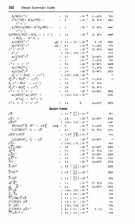
100100100100 Meson Summary Tablef0(980)π+π− < 3.8 × 10⁻⁶ CL=90% 2539ρ0 f0(980)× B(f0(980) →
π+π−) < 3 × 10⁻⁷ CL=90% 2486f0(980)f0(980)× B2(f0(980) →π+π−) < 1 × 10⁻⁷ CL=90% 2447f0(980)f0(980)× B(f0 → π+π−)
× B(f0 → K+K−) < 2.3 × 10⁻⁷ CL=90% 2447a1(1260)∓π± [gg ( 2.6 ± 0.5 )× 10−5 S=1.9 2494a2(1320)∓π± [gg < 6.3 × 10⁻⁶ CL=90% 2473π+π−π0π0 < 3.1 × 10⁻³ CL=90% 2622
ρ+ρ− ( 2.42± 0.31)× 10−5 2523a1(1260)0π0 < 1.1 × 10⁻³ CL=90% 2495ωπ0 < 5 × 10⁻⁷ CL=90% 2580
π+π+π−π−π0 < 9.0 × 10⁻³ CL=90% 2609a1(1260)+ρ− < 6.1 × 10⁻⁵ CL=90% 2433a1(1260)0 ρ0 < 2.4 × 10⁻³ CL=90% 2433b∓1 π±× B(b∓1 → ωπ∓) ( 1.09± 0.15)× 10−5 b01π0× B(b01 → ωπ0) < 1.9 × 10⁻⁶ CL=90% b−1 ρ+× B(b−1 → ωπ−) < 1.4 × 10⁻⁶ CL=90% b01 ρ0× B(b01 → ωπ0) < 3.4 × 10⁻⁶ CL=90% π+π+π+π−π−π− < 3.0 × 10⁻³ CL=90% 2592a1(1260)+a1(1260)−×B2(a+1 → 2π+π−) ( 1.18± 0.31)× 10−5 2336π+π+π+π−π−π−π0 < 1.1 % CL=90% 2572Baryon modesBaryon modesBaryon modesBaryon modespp ( 1.5 + 0.7
− 0.5 )× 10−8 2467ppπ+π− < 2.5 × 10⁻⁴ CL=90% 2406ppK0 ( 2.66± 0.32)× 10−6 2347(1540)+p, + → pK0S [aa < 5 × 10⁻⁸ CL=90% 2318fJ (2220)K0, fJ → pp < 4.5 × 10⁻⁷ CL=90% 2135ppK∗(892)0 ( 1.24+ 0.28− 0.25)× 10−6 2216fJ (2220)K∗0, fJ → pp < 1.5 × 10⁻⁷ CL=90% pπ− ( 3.14± 0.29)× 10−6 2401p (1385)− < 2.6 × 10⁻⁷ CL=90% 23630 < 9.3 × 10⁻⁷ CL=90% 2364pK− < 8.2 × 10⁻⁷ CL=90% 2308p0π− < 3.8 × 10⁻⁶ CL=90% 2383 < 3.2 × 10⁻⁷ CL=90% 2392K0 ( 4.8 + 1.0− 0.9 )× 10−6 2250K∗0 ( 2.5 + 0.9− 0.8 )× 10−6 2098D0 ( 1.1 + 0.6− 0.5 )× 10−5 166100 < 1.5 × 10⁻³ CL=90% 2335++−− < 1.1 × 10⁻⁴ CL=90% 2335D0 pp ( 1.04± 0.07)× 10−4 1863D−s p ( 2.8 ± 0.9 )× 10−5 1710D∗(2007)0 pp ( 9.9 ± 1.1 )× 10−5 1788D∗(2010)− pn ( 1.4 ± 0.4 )× 10−3 1785D− ppπ+ ( 3.32± 0.31)× 10−4 1786D∗(2010)− ppπ+ ( 4.7 ± 0.5 )× 10−4 S=1.2 1707D0 ppπ+π− ( 3.0 ± 0.5 )× 10−4 1708
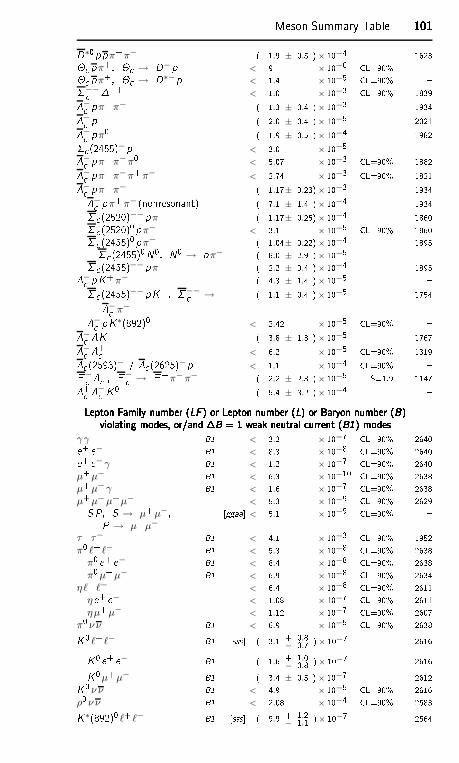
Meson Summary Table 101101101101D∗0ppπ+π− ( 1.9 ± 0.5 )× 10−4 1623 pπ+, → D−p < 9 × 10⁻⁶ CL=90% pπ+, → D∗−p < 1.4 × 10⁻⁵ CL=90% −− ++ < 1.0 × 10⁻³ CL=90% 1839− pπ+π− ( 1.3 ± 0.4 )× 10−3 1934− p ( 2.0 ± 0.4 )× 10−5 2021− pπ0 ( 1.9 ± 0.5 )× 10−4 1982 (2455)− p < 3.0 × 10⁻⁵ − pπ+π−π0 < 5.07 × 10⁻³ CL=90% 1882− pπ+π−π+π− < 2.74 × 10⁻³ CL=90% 1821− pπ+π− ( 1.17± 0.23)× 10−3 1934− pπ+π− (nonresonant) ( 7.1 ± 1.4 )× 10−4 1934 (2520)−− pπ+ ( 1.17± 0.25)× 10−4 1860 (2520)0 pπ− < 3.1 × 10⁻⁵ CL=90% 1860 (2455)0 pπ− ( 1.04± 0.22)× 10−4 1895 (2455)0N0, N0 → pπ− ( 8.0 ± 2.9 )× 10−5 (2455)−− pπ+ ( 2.2 ± 0.4 )× 10−4 1895− pK+π− ( 4.3 ± 1.4 )× 10−5 (2455)−− pK+, −− →− π−( 1.1 ± 0.4 )× 10−5 1754− pK∗(892)0 < 2.42 × 10⁻⁵ CL=90% − K+ ( 3.8 ± 1.3 )× 10−5 1767− + < 6.2 × 10⁻⁵ CL=90% 1319 (2593)− / (2625)−p < 1.1 × 10⁻⁴ CL=90% − + , − → +π−π− ( 2.2 ± 2.3 )× 10−5 S=1.9 1147+ − K0 ( 5.4 ± 3.2 )× 10−4 Lepton Family number (LF ) or Lepton number (L) or Baryon number (B)Lepton Family number (LF ) or Lepton number (L) or Baryon number (B)Lepton Family number (LF ) or Lepton number (L) or Baryon number (B)Lepton Family number (LF ) or Lepton number (L) or Baryon number (B)violating modes, or/and B = 1 weak neutral urrent (B1) modesviolating modes, or/and B = 1 weak neutral urrent (B1) modesviolating modes, or/and B = 1 weak neutral urrent (B1) modesviolating modes, or/and B = 1 weak neutral urrent (B1) modes
γ γ B1 < 3.2 × 10⁻⁷ CL=90% 2640e+ e− B1 < 8.3 × 10⁻⁸ CL=90% 2640e+ e−γ B1 < 1.2 × 10⁻⁷ CL=90% 2640µ+µ− B1 < 6.3 × 10⁻¹⁰ CL=90% 2638µ+µ− γ B1 < 1.6 × 10⁻⁷ CL=90% 2638µ+µ−µ+µ− < 5.3 × 10⁻⁹ CL=90% 2629S P , S → µ+µ−,P → µ+µ−
[ggaa < 5.1 × 10⁻⁹ CL=90% τ+ τ− B1 < 4.1 × 10⁻³ CL=90% 1952π0 ℓ+ ℓ− B1 < 5.3 × 10⁻⁸ CL=90% 2638
π0 e+ e− B1 < 8.4 × 10⁻⁸ CL=90% 2638π0µ+µ− B1 < 6.9 × 10⁻⁸ CL=90% 2634
ηℓ+ ℓ− < 6.4 × 10⁻⁸ CL=90% 2611ηe+ e− < 1.08 × 10⁻⁷ CL=90% 2611ηµ+µ− < 1.12 × 10⁻⁷ CL=90% 2607
π0 ν ν B1 < 6.9 × 10⁻⁵ CL=90% 2638K0 ℓ+ ℓ− B1 [sss ( 3.1 + 0.8− 0.7 )× 10−7 2616K0 e+ e− B1 ( 1.6 + 1.0− 0.8 )× 10−7 2616K0µ+µ− B1 ( 3.4 ± 0.5 )× 10−7 2612K0ν ν B1 < 4.9 × 10⁻⁵ CL=90% 2616
ρ0 ν ν B1 < 2.08 × 10⁻⁴ CL=90% 2583K∗(892)0 ℓ+ ℓ− B1 [sss ( 9.9 + 1.2− 1.1 )× 10−7 2564
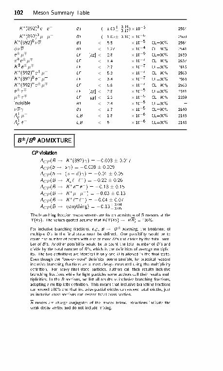
102102102102 Meson Summary TableK∗(892)0 e+ e− B1 ( 1.03+ 0.19− 0.17)× 10−6 2564K∗(892)0µ+µ− B1 ( 1.05± 0.10)× 10−6 2560K∗(892)0 ν ν B1 < 5.5 × 10⁻⁵ CL=90% 2564
φν ν B1 < 1.27 × 10⁻⁴ CL=90% 2541e±µ∓ LF [gg < 2.8 × 10⁻⁹ CL=90% 2639π0 e±µ∓ LF < 1.4 × 10⁻⁷ CL=90% 2637K0 e±µ∓ LF < 2.7 × 10⁻⁷ CL=90% 2615K∗(892)0 e+µ− LF < 5.3 × 10⁻⁷ CL=90% 2563K∗(892)0 e−µ+ LF < 3.4 × 10⁻⁷ CL=90% 2563K∗(892)0 e±µ∓ LF < 5.8 × 10⁻⁷ CL=90% 2563e± τ∓ LF [gg < 2.8 × 10⁻⁵ CL=90% 2341µ± τ∓ LF [gg < 2.2 × 10⁻⁵ CL=90% 2339invisible B1 < 2.4 × 10⁻⁵ CL=90% ν ν γ B1 < 1.7 × 10⁻⁵ CL=90% 2640+ µ− L,B < 1.8 × 10⁻⁶ CL=90% 2143+ e− L,B < 5 × 10⁻⁶ CL=90% 2145B±/B0 ADMIXTUREB±/B0 ADMIXTUREB±/B0 ADMIXTUREB±/B0 ADMIXTURECP violationCP violationCP violationCP violationACP (B → K∗(892)γ) = −0.003 ± 0.017ACP (b → s γ) = −0.008 ± 0.029ACP (b → (s + d)γ) = −0.01 ± 0.05ACP (B → Xs ℓ+ ℓ−) = −0.22 ± 0.26ACP (B → K∗ e+ e−) = −0.18 ± 0.15ACP (B → K∗µ+µ−) = −0.03 ± 0.13ACP (B → K∗ ℓ+ ℓ−) = −0.04 ± 0.07ACP (B → ηanything) = −0.13+0.04
−0.05The bran hing fra tion measurements are for an admixture of B mesons at the(4S). The values quoted assume that B((4S) → BB) = 100%.For in lusive bran hing fra tions, e.g., B → D± anything, the treatment ofmultiple D's in the nal state must be dened. One possibility would be to ount the number of events with one-or-more D's and divide by the total num-ber of B's. Another possibility would be to ount the total number of D's anddivide by the total number of B's, whi h is the denition of average multipli -ity. The two denitions are identi al if only one D is allowed in the nal state.Even though the \one-or-more" denition seems sensible, for pra ti al reasonsin lusive bran hing fra tions are almost always measured using the multipli itydenition. For heavy nal state parti les, authors all their results in lusivebran hing fra tions while for light parti les some authors all their results mul-tipli ities. In the B se tions, we list all results as in lusive bran hing fra tions,adopting a multipli ity denition. This means that in lusive bran hing fra tions an ex eed 100% and that in lusive partial widths an ex eed total widths, justas in lusive ross se tions an ex eed total ross se tion.B modes are harge onjugates of the modes below. Rea tions indi ate theweak de ay vertex and do not in lude mixing.
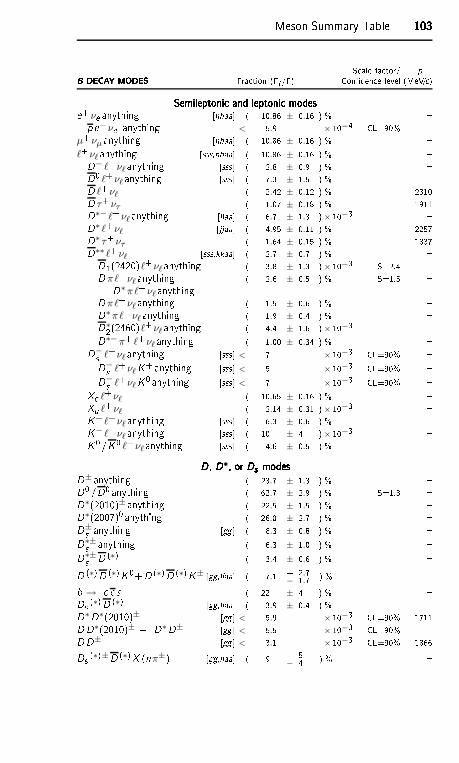
Meson Summary Table 103103103103S ale fa tor/ pB DECAY MODESB DECAY MODESB DECAY MODESB DECAY MODES Fra tion (i /) Conden e level (MeV/ )Semileptoni and leptoni modesSemileptoni and leptoni modesSemileptoni and leptoni modesSemileptoni and leptoni modese+ νe anything [hhaa ( 10.86 ± 0.16 ) % p e+νe anything < 5.9 × 10⁻⁴ CL=90% µ+νµ anything [hhaa ( 10.86 ± 0.16 ) % ℓ+νℓ anything [sss,hhaa ( 10.86 ± 0.16 ) % D− ℓ+νℓ anything [sss ( 2.8 ± 0.9 ) % D0 ℓ+νℓ anything [sss ( 7.3 ± 1.5 ) % D ℓ+νℓ ( 2.42 ± 0.12 ) % 2310D τ+ ντ ( 1.07 ± 0.18 ) % 1911D∗− ℓ+νℓ anything [iiaa ( 6.7 ± 1.3 )× 10−3 D∗ ℓ+νℓ [jjaa ( 4.95 ± 0.11 ) % 2257D∗ τ+ ντ ( 1.64 ± 0.15 ) % 1837D∗∗ ℓ+νℓ [sss,kkaa ( 2.7 ± 0.7 ) % D1(2420)ℓ+νℓ anything ( 3.8 ± 1.3 )× 10−3 S=2.4 D πℓ+νℓ anything +D∗πℓ+ νℓ anything ( 2.6 ± 0.5 ) % S=1.5 D πℓ+νℓ anything ( 1.5 ± 0.6 ) % D∗πℓ+ νℓ anything ( 1.9 ± 0.4 ) % D∗2(2460)ℓ+νℓ anything ( 4.4 ± 1.6 )× 10−3 D∗−π+ ℓ+νℓ anything ( 1.00 ± 0.34 ) % D−s ℓ+νℓ anything [sss < 7 × 10⁻³ CL=90% D−s ℓ+νℓK+ anything [sss < 5 × 10⁻³ CL=90% D−s ℓ+νℓK0 anything [sss < 7 × 10⁻³ CL=90% X ℓ+νℓ ( 10.65 ± 0.16 ) % Xu ℓ+νℓ ( 2.14 ± 0.31 )× 10−3 K+ ℓ+νℓ anything [sss ( 6.3 ± 0.6 ) % K− ℓ+νℓ anything [sss ( 10 ± 4 )× 10−3 K0/K0 ℓ+νℓ anything [sss ( 4.6 ± 0.5 ) % D, D∗, or Ds modesD, D∗, or Ds modesD, D∗, or Ds modesD, D∗, or Ds modesD± anything ( 23.7 ± 1.3 ) % D0 /D0 anything ( 62.7 ± 2.9 ) % S=1.3 D∗(2010)± anything ( 22.5 ± 1.5 ) % D∗(2007)0 anything ( 26.0 ± 2.7 ) % D±s anything [gg ( 8.3 ± 0.8 ) % D∗±s anything ( 6.3 ± 1.0 ) % D∗±s D (∗) ( 3.4 ± 0.6 ) % D (∗)D (∗)K0+D (∗)D (∗)K± [gg,llaa ( 7.1 + 2.7
− 1.7 ) % b → s ( 22 ± 4 ) % Ds (∗)D (∗) [gg,llaa ( 3.9 ± 0.4 ) % D∗D∗(2010)± [gg < 5.9 × 10⁻³ CL=90% 1711DD∗(2010)± + D∗D± [gg < 5.5 × 10⁻³ CL=90% DD± [gg < 3.1 × 10⁻³ CL=90% 1866Ds (∗)±D (∗)X (nπ±) [gg,llaa ( 9 + 5− 4 ) %
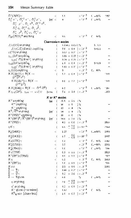
104104104104 Meson Summary TableD∗(2010)γ < 1.1 × 10⁻³ CL=90% 2257D+s π− , D∗+s π− , D+s ρ− ,D∗+s ρ− , D+s π0 , D∗+s π0 ,D+s η , D∗+s η , D+s ρ0 ,D∗+s ρ0 , D+s ω , D∗+s ω
[gg < 4 × 10⁻⁴ CL=90% Ds1(2536)+anything < 9.5 × 10⁻³ CL=90% Charmonium modesCharmonium modesCharmonium modesCharmonium modesJ/ψ(1S)anything ( 1.094± 0.032) % S=1.1 J/ψ(1S)(dire t) anything ( 7.8 ± 0.4 )× 10−3 S=1.1 ψ(2S)anything ( 3.07 ± 0.21 )× 10−3 χ 1(1P)anything ( 3.86 ± 0.27 )× 10−3
χ 1(1P)(dire t) anything ( 3.24 ± 0.25 )× 10−3 χ 2(1P)anything ( 1.4 ± 0.4 )× 10−3 S=1.9
χ 2(1P)(dire t) anything ( 1.65 ± 0.31 )× 10−3 η (1S)anything < 9 × 10⁻³ CL=90% K X (3872)× B(X →D0D0π0) ( 1.2 ± 0.4 )× 10−4 1141K X (3872)× B(X →D∗0D0) ( 8.0 ± 2.2 )× 10−5 1141K X (3940)× B(X → D∗0D0) < 6.7 × 10⁻⁵ CL=90% 1084K χ 0(2P), χ 0 → ωJ/ψ [nnaa ( 7.1 ± 3.4 )× 10−5 1103K or K∗ modesK or K∗ modesK or K∗ modesK or K∗ modesK± anything [gg ( 78.9 ± 2.5 ) % K+ anything ( 66 ± 5 ) % K− anything ( 13 ± 4 ) % K0/K0 anything [gg ( 64 ± 4 ) % K∗(892)± anything ( 18 ± 6 ) % K∗(892)0 /K∗(892)0 anything [gg ( 14.6 ± 2.6 ) % K∗(892)γ ( 4.2 ± 0.6 )× 10−5 2564ηK γ ( 8.5 + 1.8
− 1.6 )× 10−6 2588K1(1400)γ < 1.27 × 10⁻⁴ CL=90% 2453K∗2(1430)γ ( 1.7 + 0.6− 0.5 )× 10−5 2447K2(1770)γ < 1.2 × 10⁻³ CL=90% 2342K∗3(1780)γ < 3.7 × 10⁻⁵ CL=90% 2341K∗4(2045)γ < 1.0 × 10⁻³ CL=90% 2244K η′(958) ( 8.3 ± 1.1 )× 10−5 2528K∗(892)η′(958) ( 4.1 ± 1.1 )× 10−6 2472K η < 5.2 × 10⁻⁶ CL=90% 2588K∗(892)η ( 1.8 ± 0.5 )× 10−5 2534K φφ ( 2.3 ± 0.9 )× 10−6 2306b → s γ ( 3.40 ± 0.21 )× 10−4 b → d γ ( 9.2 ± 3.0 )× 10−6 b → s gluon < 6.8 % CL=90%
η anything ( 2.6 + 0.5− 0.8 )× 10−4
η′ anything ( 4.2 ± 0.9 )× 10−4 K+gluon ( harmless) < 1.87 × 10⁻⁴ CL=90% K0gluon ( harmless) ( 1.9 ± 0.7 )× 10−4
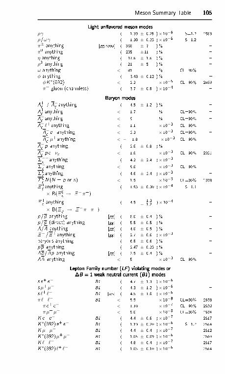
Meson Summary Table 105105105105Light un avored meson modesLight un avored meson modesLight un avored meson modesLight un avored meson modesργ ( 1.39 ± 0.25 )× 10−6 S=1.2 2583ρ/ωγ ( 1.30 ± 0.23 )× 10−6 S=1.2 π± anything [gg,ooaa ( 358 ± 7 ) % π0 anything ( 235 ±11 ) % η anything ( 17.6 ± 1.6 ) % ρ0 anything ( 21 ± 5 ) % ω anything < 81 % CL=90% φ anything ( 3.43 ± 0.12 ) %
φK∗(892) < 2.2 × 10⁻⁵ CL=90% 2460π+ gluon ( harmless) ( 3.7 ± 0.8 )× 10−4 Baryon modesBaryon modesBaryon modesBaryon modes+ / − anything ( 4.5 ± 1.2 ) % + anything < 1.7 % CL=90% − anything < 9 % CL=90% − ℓ+anything < 1.1 × 10⁻³ CL=90% − e+ anything < 2.3 × 10⁻³ CL=90% − µ+ anything < − 1.8 × 10⁻³ CL=90% − p anything ( 2.6 ± 0.8 ) % − p e+νe < 1.0 × 10⁻³ CL=90% 2021−− anything ( 4.2 ± 2.4 )× 10−3 − anything < 9.6 × 10⁻³ CL=90% 0 anything ( 4.6 ± 2.4 )× 10−3 0 N (N = p or n) < 1.5 × 10⁻³ CL=90% 1938 0 anything× B( 0 → −π+) ( 1.93 ± 0.30 )× 10−4 S=1.1 + anything× B(+ → −π+π+) ( 4.5 + 1.3
− 1.2 )× 10−4 p/p anything [gg ( 8.0 ± 0.4 ) % p/p (dire t) anything [gg ( 5.5 ± 0.5 ) % / anything [gg ( 4.0 ± 0.5 ) % −/+ anything [gg ( 2.7 ± 0.6 )× 10−3 baryons anything ( 6.8 ± 0.6 ) % pp anything ( 2.47 ± 0.23 ) % p/p anything [gg ( 2.5 ± 0.4 ) % anything < 5 × 10⁻³ CL=90% Lepton Family number (LF ) violating modes orLepton Family number (LF ) violating modes orLepton Family number (LF ) violating modes orLepton Family number (LF ) violating modes orB = 1 weak neutral urrent (B1) modesB = 1 weak neutral urrent (B1) modesB = 1 weak neutral urrent (B1) modesB = 1 weak neutral urrent (B1) modess e+ e− B1 ( 4.7 ± 1.3 )× 10−6 sµ+µ− B1 ( 4.3 ± 1.2 )× 10−6 s ℓ+ ℓ− B1 [sss ( 4.5 ± 1.0 )× 10−6 πℓ+ ℓ− B1 < 5.9 × 10⁻⁸ CL=90% 2638
πe+ e− < 1.10 × 10⁻⁷ CL=90% 2638πµ+µ− < 5.0 × 10⁻⁸ CL=90% 2634K e+ e− B1 ( 4.4 ± 0.6 )× 10−7 2617K∗(892)e+ e− B1 ( 1.19 ± 0.20 )× 10−6 S=1.2 2564K µ+µ− B1 ( 4.4 ± 0.4 )× 10−7 2612K∗(892)µ+µ− B1 ( 1.06 ± 0.09 )× 10−6 2560K ℓ+ ℓ− B1 ( 4.8 ± 0.4 )× 10−7 2617K∗(892)ℓ+ ℓ− B1 ( 1.05 ± 0.10 )× 10−6 2564
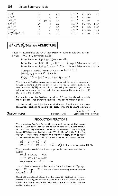
106106106106 Meson Summary TableK ν ν B1 < 1.7 × 10⁻⁵ CL=90% 2617K∗ν ν B1 < 7.6 × 10⁻⁵ CL=90% s e±µ∓ LF [gg < 2.2 × 10⁻⁵ CL=90% πe±µ∓ LF < 9.2 × 10⁻⁸ CL=90% 2637ρe±µ∓ LF < 3.2 × 10⁻⁶ CL=90% 2582K e±µ∓ LF < 3.8 × 10⁻⁸ CL=90% 2616K∗(892)e±µ∓ LF < 5.1 × 10⁻⁷ CL=90% 2563B±/B0/B0s/b-baryon ADMIXTUREB±/B0/B0s/b-baryon ADMIXTUREB±/B0/B0s/b-baryon ADMIXTUREB±/B0/B0s/b-baryon ADMIXTUREThese measurements are for an admixture of bottom parti les at highenergy (LHC, LEP, Tevatron, SppS).Mean life τ = (1.568 ± 0.009)× 10−12 sMean life τ = (1.72± 0.10)×10−12 s Charged b-hadron admixtureMean life τ = (1.58 ± 0.14)× 10−12 s Neutral b-hadron admixture
τ harged b−hadron/τ neutral b−hadron = 1.09 ± 0.13∣
∣τ b∣∣/τ b,b = −0.001 ± 0.014Re(ǫb) / (1 + ∣
∣ǫb∣∣2) = (1.2 ± 0.4)× 10−3The bran hing fra tion measurements are for an admixture of B mesons andbaryons at energies above the (4S). Only the highest energy results (LHC,LEP, Tevatron, SppS) are used in the bran hing fra tion averages. In thefollowing, we assume that the produ tion fra tions are the same at the LHC,LEP, and at the Tevatron.For in lusive bran hing fra tions, e.g., B → D± anything, the values usuallyare multipli ities, not bran hing fra tions. They an be greater than one.The modes below are listed for a b initial state. bmodes are their harge onjugates. Rea tions indi ate the weak de ay vertex and do not in lude mixing.S ale fa tor/ pb DECAY MODESb DECAY MODESb DECAY MODESb DECAY MODES Fra tion (i /) Conden e level (MeV/ )PRODUCTION FRACTIONSPRODUCTION FRACTIONSPRODUCTION FRACTIONSPRODUCTION FRACTIONSThe produ tion fra tions for weakly de aying b-hadrons at high energyhave been al ulated from the best values of mean lives, mixing parame-ters, and bran hing fra tions in this edition by the Heavy Flavor AveragingGroup (HFAG) as des ribed in the note \B0-B0 Mixing" in the B0 Parti leListings. The produ tion fra tions in b-hadroni Z de ay or pp ollisionsat the Tevatron are also listed at the end of the se tion. Values assumeB(b → B+) = B(b → B0)B(b → B+) + B(b → B0) +B(b → B0s ) + B(b → b -baryon) = 100 %.The orrelation oeÆ ients between produ tion fra tions are also re-ported: or(B0s , b-baryon) = −0.291 or(B0s , B±=B0) = −0.083 or(b-baryon, B±=B0) = −0.929.The notation for produ tion fra tions varies in the literature (fd , dB0 ,f (b → B0), Br(b → B0)). We use our own bran hing fra tion notationhere, B(b → B0).Note these produ tion fra tions are b-hadronization fra tions, not the on-ventional bran hing fra tions of b-quark to a B-hadron, whi h may have onsiderable dependen e on the initial and nal state kinemati and pro-du tion environment.
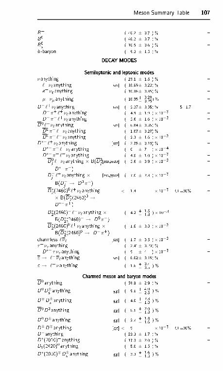
Meson Summary Table 107107107107B+ ( 40.2 ± 0.7 ) % B0 ( 40.2 ± 0.7 ) % B0s ( 10.5 ± 0.6 ) % b -baryon ( 9.2 ± 1.5 ) % DECAY MODESDECAY MODESDECAY MODESDECAY MODESSemileptoni and leptoni modesSemileptoni and leptoni modesSemileptoni and leptoni modesSemileptoni and leptoni modesν anything ( 23.1 ± 1.5 ) %
ℓ+νℓ anything [sss ( 10.69± 0.22) % e+ νe anything ( 10.86± 0.35) % µ+νµ anything ( 10.95+ 0.29
− 0.25) % D− ℓ+νℓ anything [sss ( 2.27± 0.35) % S=1.7 D−π+ ℓ+νℓ anything ( 4.9 ± 1.9 )× 10−3 D−π− ℓ+νℓ anything ( 2.6 ± 1.6 )× 10−3 D0 ℓ+νℓ anything [sss ( 6.84± 0.35) % D0π− ℓ+νℓ anything ( 1.07± 0.27) % D0π+ ℓ+νℓ anything ( 2.3 ± 1.6 )× 10−3 D∗− ℓ+νℓ anything [sss ( 2.75± 0.19) % D∗−π− ℓ+νℓ anything ( 6 ± 7 )× 10−4 D∗−π+ ℓ+νℓ anything ( 4.8 ± 1.0 )× 10−3 D0j ℓ+νℓ anything × B(D0j →D∗+π−) [sss,ppaa ( 2.6 ± 0.9 )× 10−3 D−j ℓ+νℓ anything ×B(D−j → D0π−) [sss,ppaa ( 7.0 ± 2.3 )× 10−3 D∗2(2460)0 ℓ+νℓ anything× B(D∗2(2460)0 →D∗−π+) < 1.4 × 10⁻³ CL=90% D∗2(2460)− ℓ+νℓ anything ×B(D∗2(2460)− → D0π−) ( 4.2 + 1.5
− 1.8 )× 10−3 D∗2(2460)0 ℓ+νℓ anything ×B(D∗2(2460)0 → D−π+) ( 1.6 ± 0.8 )× 10−3 harmless ℓνℓ [sss ( 1.7 ± 0.5 )× 10−3 τ+ ντ anything ( 2.41± 0.23) % D∗− τ ντ anything ( 9 ± 4 )× 10−3 → ℓ−νℓ anything [sss ( 8.02± 0.19) % → ℓ+ν anything ( 1.6 + 0.4
− 0.5 ) % Charmed meson and baryon modesCharmed meson and baryon modesCharmed meson and baryon modesCharmed meson and baryon modesD0 anything ( 59.8 ± 2.9 ) % D0D±s anything [gg ( 9.1 + 4.0− 2.8 ) % D∓D±s anything [gg ( 4.0 + 2.3− 1.8 ) % D0D0 anything [gg ( 5.1 + 2.0− 1.8 ) % D0D± anything [gg ( 2.7 + 1.8− 1.6 ) % D±D∓ anything [gg < 9 × 10⁻³ CL=90% D− anything ( 23.3 ± 1.7 ) % D∗(2010)+ anything ( 17.3 ± 2.0 ) % D1(2420)0 anything ( 5.0 ± 1.5 ) % D∗(2010)∓D±s anything [gg ( 3.3 + 1.6− 1.3 ) %
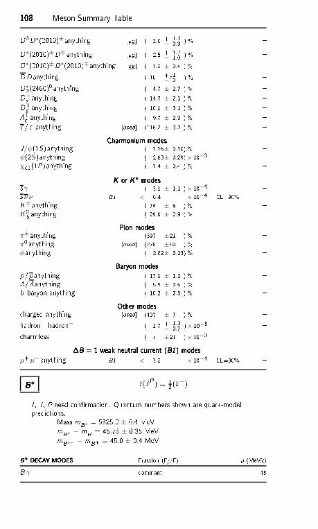
108108108108 Meson Summary TableD0D∗(2010)± anything [gg ( 3.0 + 1.1− 0.9 ) % D∗(2010)±D∓ anything [gg ( 2.5 + 1.2− 1.0 ) % D∗(2010)±D∗(2010)∓ anything [gg ( 1.2 ± 0.4 ) % DD anything ( 10 +11−10 ) % D∗2(2460)0 anything ( 4.7 ± 2.7 ) % D−s anything ( 14.7 ± 2.1 ) % D+s anything ( 10.1 ± 3.1 ) % + anything ( 9.7 ± 2.9 ) % / anything [ooaa (116.2 ± 3.2 ) % Charmonium modesCharmonium modesCharmonium modesCharmonium modesJ/ψ(1S)anything ( 1.16± 0.10) %
ψ(2S)anything ( 2.83± 0.29)× 10−3 χ 1(1P)anything ( 1.4 ± 0.4 ) % K or K∗ modesK or K∗ modesK or K∗ modesK or K∗ modess γ ( 3.1 ± 1.1 )× 10−4 s ν ν B1 < 6.4 × 10⁻⁴ CL=90% K± anything ( 74 ± 6 ) % K0S anything ( 29.0 ± 2.9 ) % Pion modesPion modesPion modesPion modesπ± anything (397 ±21 ) % π0 anything [ooaa (278 ±60 ) % φanything ( 2.82± 0.23) % Baryon modesBaryon modesBaryon modesBaryon modesp/p anything ( 13.1 ± 1.1 ) % /anything ( 5.9 ± 0.6 ) % b -baryon anything ( 10.2 ± 2.8 ) % Other modesOther modesOther modesOther modes harged anything [ooaa (497 ± 7 ) % hadron+ hadron− ( 1.7 + 1.0
− 0.7 )× 10−5 harmless ( 7 ±21 )× 10−3 B = 1 weak neutral urrent (B1) modesB = 1 weak neutral urrent (B1) modesB = 1 weak neutral urrent (B1) modesB = 1 weak neutral urrent (B1) modesµ+µ− anything B1 < 3.2 × 10⁻⁴ CL=90% B∗B∗B∗B∗ I (JP ) = 12 (1−)I , J , P need onrmation. Quantum numbers shown are quark-modelpredi tions.Mass mB∗ = 5325.2 ± 0.4 MeVmB∗ − mB = 45.78 ± 0.35 MeVmB∗+ − mB+ = 45.0 ± 0.4 MeVB∗ DECAY MODESB∗ DECAY MODESB∗ DECAY MODESB∗ DECAY MODES Fra tion (i /) p (MeV/ )B γ dominant 45
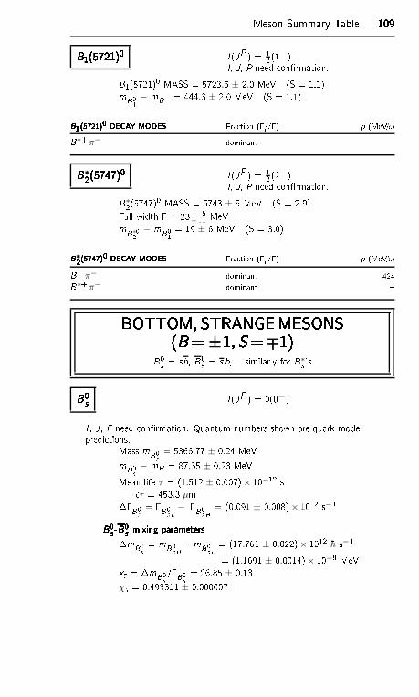
Meson Summary Table 109109109109B1(5721)0B1(5721)0B1(5721)0B1(5721)0 I (JP ) = 12 (1+)I, J, P need onrmation.B1(5721)0 MASS = 5723.5 ± 2.0 MeV (S = 1.1)mB01 − mB+ = 444.3 ± 2.0 MeV (S = 1.1)B1(5721)0 DECAY MODESB1(5721)0 DECAY MODESB1(5721)0 DECAY MODESB1(5721)0 DECAY MODES Fra tion (i /) p (MeV/ )B∗+π− dominant B∗2(5747)0B∗2(5747)0B∗2(5747)0B∗2(5747)0 I (JP ) = 12 (2+)I, J, P need onrmation.B∗2(5747)0 MASS = 5743 ± 5 MeV (S = 2.9)Full width = 23+ 5−11 MeVmB∗02 − mB01 = 19 ± 6 MeV (S = 3.0)B∗2(5747)0 DECAY MODESB∗2(5747)0 DECAY MODESB∗2(5747)0 DECAY MODESB∗2(5747)0 DECAY MODES Fra tion (i /) p (MeV/ )B+π− dominant 424B∗+π− dominant BOTTOM, STRANGEMESONSBOTTOM, STRANGEMESONSBOTTOM, STRANGEMESONSBOTTOM, STRANGEMESONS(B= ±1, S=∓1)(B= ±1, S=∓1)(B= ±1, S=∓1)(B= ±1, S=∓1)B0s = sb, B0s = s b, similarly for B∗s 'sB0sB0sB0sB0s I (JP ) = 0(0−)I , J , P need onrmation. Quantum numbers shown are quark-modelpredi tions.Mass mB0s = 5366.77 ± 0.24 MeVmB0s − mB = 87.35 ± 0.23 MeVMean life τ = (1.512 ± 0.007)× 10−12 s τ = 453.3 µmB0s = B0s L − B0s H = (0.091 ± 0.008)× 1012 s−1B0s -B0s mixing parametersB0s -B0s mixing parametersB0s -B0s mixing parametersB0s -B0s mixing parametersmB0s = mB0s H mB0s L = (17.761 ± 0.022)× 1012 h s−1= (1.1691 ± 0.0014)× 10−8 MeVxs = mB0s /B0s = 26.85 ± 0.13
χs = 0.499311 ± 0.000007
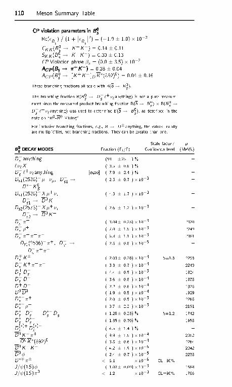
110110110110 Meson Summary TableCP violation parameters in B0sCP violation parameters in B0sCP violation parameters in B0sCP violation parameters in B0sRe(ǫB0s ) / (1 + ∣
∣ǫB0s ∣∣2) = (−1.9 ± 1.0)× 10−3CK K (B0s → K+K−) = 0.14 ± 0.11SK K (B0s → K+K−) = 0.30 ± 0.13CP Violation phase βs = (0.0 ± 3.5)× 10−2ACP (Bs → π+K−)ACP (Bs → π+K−)ACP (Bs → π+K−)ACP (Bs → π+K−) = 0.28 ± 0.04ACP (B0s → [K+K− DK∗(892)0) = 0.04 ± 0.16These bran hing fra tions all s ale with B(b → B0s ).The bran hing fra tion B(B0s → D−s ℓ+ νℓ anything) is not a pure measure-ment sin e the measured produ t bran hing fra tion B(b → B0s ) × B(B0s →D−s ℓ+ νℓ anything) was used to determine B(b → B0s ), as des ribed in thenote on \B0-B0 Mixing"For in lusive bran hing fra tions, e.g., B → D± anything, the values usuallyare multipli ities, not bran hing fra tions. They an be greater than one.S ale fa tor/ pB0s DECAY MODESB0s DECAY MODESB0s DECAY MODESB0s DECAY MODES Fra tion (i /) Conden e level (MeV/ )D−s anything (93 ±25 ) % ℓνℓX (10.5 ± 0.8 ) % D−s ℓ+νℓ anything [qqaa ( 7.9 ± 2.4 ) % Ds1(2536)−µ+ νµ, D−s1 →D∗−K0S ( 2.5 ± 0.7 )× 10−3 Ds1(2536)−X µ+ν,D−s1 → D0K+ ( 4.3 ± 1.7 )× 10−3 Ds2(2573)−X µ+ν,D−s2 → D0K+ ( 2.6 ± 1.2 )× 10−3 D−s π+ ( 3.04± 0.23)× 10−3 2320D−s ρ+ ( 7.0 ± 1.5 )× 10−3 2249D−s π+π+π− ( 6.3 ± 1.1 )× 10−3 2301Ds1(2536)−π+, D−s1 →D−s π+π−
( 2.5 ± 0.8 )× 10−5 D∓s K± ( 2.03± 0.28)× 10−4 S=1.3 2293D−s K+π+π− ( 3.3 ± 0.7 )× 10−4 2249D+s D−s ( 4.4 ± 0.5 )× 10−3 1824D−s D+ ( 3.6 ± 0.8 )× 10−4 1875D+D− ( 2.2 ± 0.6 )× 10−4 1925D0D0 ( 1.9 ± 0.5 )× 10−4 1929D∗−s π+ ( 2.0 ± 0.5 )× 10−3 2265D∗−s ρ+ ( 9.7 ± 2.2 )× 10−3 2191D∗+s D−s + D∗−s D+s ( 1.28± 0.23) % S=1.2 1742D∗+s D∗−s ( 1.85± 0.30) % 1655D(∗)+s D(∗)−s ( 4.5 ± 1.4 ) % D0K−π+ ( 9.9 ± 1.5 )× 10−4 2312D0K∗(892)0 ( 3.5 ± 0.6 )× 10−4 2264D0K+K− ( 4.2 ± 1.9 )× 10−5 2242D0φ ( 2.4 ± 0.7 )× 10−5 2235D∗∓π± < 6.1 × 10⁻⁶ CL=90% J/ψ(1S)φ ( 1.07± 0.09)× 10−3 1588J/ψ(1S)π0 < 1.2 × 10⁻³ CL=90% 1786
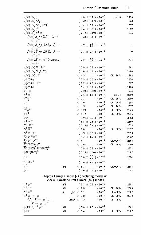
Meson Summary Table 111111111111J/ψ(1S)η ( 4.0 ± 0.7 )× 10−4 S=1.3 1733J/ψ(1S)K0S ( 1.87± 0.17)× 10−5 1743J/ψ(1S)K∗(892)0 ( 4.4 ± 0.9 )× 10−5 1637J/ψ(1S)η′ ( 3.4 ± 0.5 )× 10−4 1612J/ψ(1S)π+π− ( 2.12± 0.19)× 10−4 1775J/ψ(1S) f0(980), f0 →π+π−
( 1.39± 0.14)× 10−4 J/ψ(1S) f0(1370), f0 →π+π−
( 3.9 + 0.8− 1.8 )× 10−5 J/ψ(1S) f2(1270), f2 →
π+π−( 1.1 ± 0.4 )× 10−6 J/ψ(1S)π+π− (nonreso-nant) ( 1.8 + 1.1
− 0.4 )× 10−5 1775J/ψ(1S)K+K− ( 7.9 ± 0.7 )× 10−4 1601J/ψ(1S) f ′2(1525) ( 2.6 ± 0.6 )× 10−4 1304J/ψ(1S)pp < 4.8 × 10⁻⁶ CL=90% 982ψ(2S)η ( 3.3 ± 0.9 )× 10−4 1338ψ(2S)π+π− ( 7.2 ± 1.2 )× 10−5 1397ψ(2S)φ ( 5.4 ± 0.6 )× 10−4 1120χ 1φ ( 2.02± 0.30)× 10−4 1274π+π− ( 7.6 ± 1.9 )× 10−7 S=1.4 2680π0π0 < 2.1 × 10⁻⁴ CL=90% 2680ηπ0 < 1.0 × 10⁻³ CL=90% 2654ηη < 1.5 × 10⁻³ CL=90% 2627ρ0 ρ0 < 3.20 × 10⁻⁴ CL=90% 2569φρ0 < 6.17 × 10⁻⁴ CL=90% 2526φφ ( 1.91± 0.31)× 10−5 2482π+K− ( 5.5 ± 0.6 )× 10−6 2659K+K− ( 2.49± 0.17)× 10−5 2638K0K0 < 6.6 × 10⁻⁵ CL=90% 2637K0π+π− ( 1.9 ± 0.5 )× 10−5 2653K0K±π∓ ( 9.7 ± 1.7 )× 10−5 2622K0K+K− < 4 × 10⁻⁶ CL=90% 2568K∗(892)0 ρ0 < 7.67 × 10⁻⁴ CL=90% 2550K∗(892)0K∗(892)0 ( 2.8 ± 0.7 )× 10−5 2531φK∗(892)0 ( 1.13± 0.30)× 10−6 2507pp ( 2.8 + 2.2
− 1.7 )× 10−8 2514− π+ ( 3.6 ± 1.6 )× 10−4 γ γ B1 < 8.7 × 10⁻⁶ CL=90% 2683φγ ( 3.6 ± 0.4 )× 10−5 2587Lepton Family number (LF ) violating modes orLepton Family number (LF ) violating modes orLepton Family number (LF ) violating modes orLepton Family number (LF ) violating modes orB = 1 weak neutral urrent (B1) modesB = 1 weak neutral urrent (B1) modesB = 1 weak neutral urrent (B1) modesB = 1 weak neutral urrent (B1) modesµ+µ− B1 ( 3.1 ± 0.7 )× 10−9 2681e+ e− B1 < 2.8 × 10⁻⁷ CL=90% 2683e±µ∓ LF [gg < 1.1 × 10⁻⁸ CL=90% 2682µ+µ−µ+µ− < 1.2 × 10⁻⁸ CL=90% 2673S P , S → µ+µ−,P → µ+µ−
[ggaa < 1.2 × 10⁻⁸ CL=90% φ(1020)µ+µ− B1 ( 7.6 ± 1.5 )× 10−7 2582φν ν B1 < 5.4 × 10⁻³ CL=90% 2587
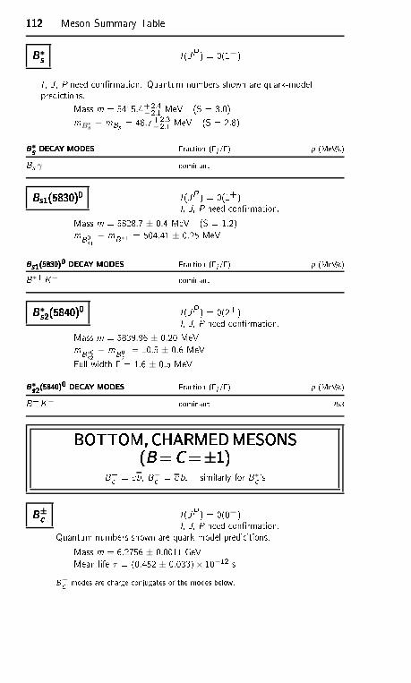
112112112112 Meson Summary TableB∗sB∗sB∗sB∗s I (JP ) = 0(1−)I , J , P need onrmation. Quantum numbers shown are quark-modelpredi tions.Mass m = 5415.4+2.4−2.1 MeV (S = 3.0)mB∗
s− mBs = 48.7+2.3
−2.1 MeV (S = 2.8)B∗s DECAY MODESB∗s DECAY MODESB∗s DECAY MODESB∗s DECAY MODES Fra tion (i /) p (MeV/ )Bs γ dominant Bs1(5830)0Bs1(5830)0Bs1(5830)0Bs1(5830)0 I (JP ) = 0(1+)I, J, P need onrmation.Mass m = 5828.7 ± 0.4 MeV (S = 1.2)mB0s1 − mB∗+ = 504.41 ± 0.25 MeVBs1(5830)0 DECAY MODESBs1(5830)0 DECAY MODESBs1(5830)0 DECAY MODESBs1(5830)0 DECAY MODES Fra tion (i /) p (MeV/ )B∗+K− dominant B∗s2(5840)0B∗s2(5840)0B∗s2(5840)0B∗s2(5840)0 I (JP ) = 0(2+)I, J, P need onrmation.Mass m = 5839.96 ± 0.20 MeVmB∗0s2 − mB0s1 = 10.5 ± 0.6 MeVFull width = 1.6 ± 0.5 MeVB∗s2(5840)0 DECAY MODESB∗s2(5840)0 DECAY MODESB∗s2(5840)0 DECAY MODESB∗s2(5840)0 DECAY MODES Fra tion (i /) p (MeV/ )B+K− dominant 253BOTTOM,CHARMEDMESONSBOTTOM,CHARMEDMESONSBOTTOM,CHARMEDMESONSBOTTOM,CHARMEDMESONS(B=C=±1)(B=C=±1)(B=C=±1)(B=C=±1)B+ = b, B− = b, similarly for B∗ 'sB± B± B± B± I (JP ) = 0(0−)I, J, P need onrmation.Quantum numbers shown are quark-model predi itions.Mass m = 6.2756 ± 0.0011 GeVMean life τ = (0.452 ± 0.033)× 10−12 sB− modes are harge onjugates of the modes below.
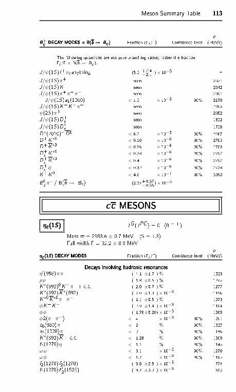
Meson Summary Table 113113113113pB+ DECAY MODES × B(b → B )B+ DECAY MODES × B(b → B )B+ DECAY MODES × B(b → B )B+ DECAY MODES × B(b → B ) Fra tion (i /) Conden e level (MeV/ )The following quantities are not pure bran hing ratios; rather the fra tioni / × B(b → B ).J/ψ(1S)ℓ+νℓ anything (5.2 +2.4−2.1 ) × 10−5 J/ψ(1S)π+ seen 2371J/ψ(1S)K+ seen 2342J/ψ(1S)π+π+π− seen 2351J/ψ(1S)a1(1260) < 1.2 × 10⁻³ 90% 2170J/ψ(1S)K+K−π+ seen 2203
ψ(2S)π+ seen 2052J/ψ(1S)D+s seen 1822J/ψ(1S)D∗+s seen 1728D∗(2010)+D0 < 6.2 × 10⁻³ 90% 2467D+K∗0 < 0.20 × 10⁻⁶ 90% 2783D+K∗0 < 0.16 × 10⁻⁶ 90% 2783D+s K∗0 < 0.28 × 10⁻⁶ 90% 2752D+s K∗0 < 0.4 × 10⁻⁶ 90% 2752D+s φ < 0.32 × 10⁻⁶ 90% 2728K+K0 < 4.6 × 10⁻⁷ 90% 3098B0s π+ / B(b → Bs ) (2.37+0.37−0.35) × 10−3 MESONS MESONS MESONS MESONS
η (1S)η (1S)η (1S)η (1S) IG (JPC ) = 0+(0−+)Mass m = 2983.6 ± 0.7 MeV (S = 1.3)Full width = 32.2 ± 0.9 MeV pη (1S) DECAY MODESη (1S) DECAY MODESη (1S) DECAY MODESη (1S) DECAY MODES Fra tion (i /) Conden e level (MeV/ )De ays involving hadroni resonan esDe ays involving hadroni resonan esDe ays involving hadroni resonan esDe ays involving hadroni resonan esη′(958)ππ ( 4.1 ±1.7 ) % 1323ρρ ( 1.8 ±0.5 ) % 1275K∗(892)0K−π++ . . ( 2.0 ±0.7 ) % 1277K∗(892)K∗(892) ( 7.0 ±1.3 )× 10−3 1196K∗0K∗0π+π− ( 1.1 ±0.5 ) % 1073φK+K− ( 2.9 ±1.4 )× 10−3 1104φφ ( 1.76±0.20)× 10−3 1089φ2(π+π−) < 4 × 10⁻³ 90% 1251a0(980)π < 2 % 90% 1327a2(1320)π < 2 % 90% 1196K∗(892)K+ . . < 1.28 % 90% 1309f2(1270)η < 1.1 % 90% 1145ωω < 3.1 × 10⁻³ 90% 1270ωφ < 1.7 × 10⁻³ 90% 1185f2(1270)f2(1270) ( 9.8 ±2.5 )× 10−3 774f2(1270)f ′2(1525) ( 9.7 ±3.2 )× 10−3 513
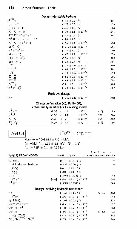
114114114114 Meson Summary TableDe ays into stable hadronsDe ays into stable hadronsDe ays into stable hadronsDe ays into stable hadronsK K π ( 7.3 ±0.5 ) % 1381ηπ+π− ( 1.7 ±0.5 ) % 1428η2(π+π−) ( 4.4 ±1.3 ) % 1385K+K−π+π− ( 6.9 ±1.1 )× 10−3 1345K+K−π+π−π0 ( 3.5 ±0.6 ) % 1304K0K−π+π−π++ . . ( 5.6 ±1.5 ) % K+K−2(π+π−) ( 7.5 ±2.4 )× 10−3 12532(K+K−) ( 1.47±0.31)× 10−3 1055π+π−π0π0 ( 4.7 ±1.0 ) % 14602(π+π−) ( 9.7 ±1.2 )× 10−3 14592(π+π−π0) (17.4 ±3.3 ) % 14093(π+π−) ( 1.8 ±0.4 ) % 1407pp ( 1.52±0.16)× 10−3 1160ppπ0 ( 3.6 ±1.3 )× 10−3 1101 ( 1.09±0.24)× 10−3 990+− ( 2.1 ±0.6 )× 10−3 901−+ ( 8.9 ±2.7 )× 10−4 692K K η (10 ±5 )× 10−3 1265π+π−pp ( 5.3 ±1.8 )× 10−3 1027Radiative de aysRadiative de aysRadiative de aysRadiative de aysγ γ ( 1.57±0.12)× 10−4 1492Charge onjugation (C), Parity (P),Charge onjugation (C), Parity (P),Charge onjugation (C), Parity (P),Charge onjugation (C), Parity (P),Lepton family number (LF) violating modesLepton family number (LF) violating modesLepton family number (LF) violating modesLepton family number (LF) violating modesπ+π− P,CP < 1.1 × 10⁻⁴ 90% 1485π0π0 P,CP < 3.5 × 10⁻⁵ 90% 1486K+K− P,CP < 6 × 10⁻⁴ 90% 1408K0S K0S P,CP < 3.1 × 10⁻⁴ 90% 1406J/ψ(1S)J/ψ(1S)J/ψ(1S)J/ψ(1S) IG (JPC ) = 0−(1−−)Mass m = 3096.916 ± 0.011 MeVFull width = 92.9 ± 2.8 keV (S = 1.1)e e = 5.55 ± 0.14 ± 0.02 keV S ale fa tor/ pJ/ψ(1S) DECAY MODESJ/ψ(1S) DECAY MODESJ/ψ(1S) DECAY MODESJ/ψ(1S) DECAY MODES Fra tion (i /) Conden e level (MeV/ )hadrons (87.7 ±0.5 ) % virtualγ → hadrons (13.50 ±0.30 ) % g g g (64.1 ±1.0 ) %
γ g g ( 8.8 ±1.1 ) % e+ e− ( 5.971±0.032) % 1548e+ e−γ [rraa ( 8.8 ±1.4 )× 10−3 1548µ+µ− ( 5.961±0.033) % 1545De ays involving hadroni resonan esDe ays involving hadroni resonan esDe ays involving hadroni resonan esDe ays involving hadroni resonan esρπ ( 1.69 ±0.15 ) % S=2.4 1448
ρ0π0 ( 5.6 ±0.7 )× 10−3 1448a2(1320)ρ ( 1.09 ±0.22 ) % 1123ωπ+π+π−π− ( 8.5 ±3.4 )× 10−3 1392ωπ+π−π0 ( 4.0 ±0.7 )× 10−3 1418ωπ+π− ( 8.6 ±0.7 )× 10−3 S=1.1 1435
ω f2(1270) ( 4.3 ±0.6 )× 10−3 1142K∗(892)0K∗(892)0 ( 2.3 ±0.7 )× 10−4 1266
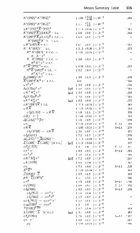
Meson Summary Table 115115115115K∗(892)±K∗(892)∓ ( 1.00 +0.22−0.40 )× 10−3 1266K∗(892)±K∗(800)∓ ( 1.1 +1.0−0.6 )× 10−3
ηK∗(892)0K∗(892)0 ( 1.15 ±0.26 )× 10−3 1003K∗(892)0K∗2(1430)0+ . . ( 6.0 ±0.6 )× 10−3 1012K∗(892)0K2(1770)0+ . . →K∗(892)0K−π++ . . ( 6.9 ±0.9 )× 10−4 ωK∗(892)K+ . . ( 6.1 ±0.9 )× 10−3 1097K+K∗(892)−+ . . ( 5.12 ±0.30 )× 10−3 1373K+K∗(892)−+ . . →K+K−π0 ( 1.97 ±0.20 )× 10−3 K+K∗(892)−+ . . →K0K±π∓+ . . ( 3.0 ±0.4 )× 10−3 K0K∗(892)0+ . . ( 4.39 ±0.31 )× 10−3 1373K0K∗(892)0+ . . →K0K±π∓+ . . ( 3.2 ±0.4 )× 10−3 K1(1400)±K∓ ( 3.8 ±1.4 )× 10−3 1170K∗(892)0K+π−+ . . seen 1343ωπ0π0 ( 3.4 ±0.8 )× 10−3 1436b1(1235)±π∓ [gg ( 3.0 ±0.5 )× 10−3 1300ωK±K0S π∓ [gg ( 3.4 ±0.5 )× 10−3 1210b1(1235)0π0 ( 2.3 ±0.6 )× 10−3 1300ηK±K0S π∓ [gg ( 2.2 ±0.4 )× 10−3 1278φK∗(892)K+ . . ( 2.18 ±0.23 )× 10−3 969ωK K ( 1.70 ±0.32 )× 10−3 1268
ω f0(1710) → ωKK ( 4.8 ±1.1 )× 10−4 878φ2(π+π−) ( 1.66 ±0.23 )× 10−3 1318(1232)++pπ− ( 1.6 ±0.5 )× 10−3 1030ωη ( 1.74 ±0.20 )× 10−3 S=1.6 1394φK K ( 1.83 ±0.24 )× 10−3 S=1.5 1179
φ f0(1710) → φK K ( 3.6 ±0.6 )× 10−4 875φ f2(1270) ( 7.2 ±1.3 )× 10−4 1036(1232)++(1232)−− ( 1.10 ±0.29 )× 10−3 938 (1385)− (1385)+ (or . .) [gg ( 1.10 ±0.12 )× 10−3 697φ f ′2(1525) ( 8 ±4 )× 10−4 S=2.7 871φπ+π− ( 9.4 ±0.9 )× 10−4 S=1.2 1365φπ0π0 ( 5.6 ±1.6 )× 10−4 1366φK±K0S π∓ [gg ( 7.2 ±0.8 )× 10−4 1114ω f1(1420) ( 6.8 ±2.4 )× 10−4 1062φη ( 7.5 ±0.8 )× 10−4 S=1.5 1320 0 0 ( 1.20 ±0.24 )× 10−3 818 (1530)−+ ( 5.9 ±1.5 )× 10−4 600pK− (1385)0 ( 5.1 ±3.2 )× 10−4 646ωπ0 ( 4.5 ±0.5 )× 10−4 S=1.4 1446φη′(958) ( 4.0 ±0.7 )× 10−4 S=2.1 1192φ f0(980) ( 3.2 ±0.9 )× 10−4 S=1.9 1178
φ f0(980) → φπ+π− ( 1.8 ±0.4 )× 10−4 φ f0(980) → φπ0π0 ( 1.7 ±0.7 )× 10−4
ηφ f0(980) → ηφπ+π− ( 3.2 ±1.0 )× 10−4 φa0(980)0 → φηπ0 ( 5 ±4 )× 10−6 (1530)0 0 ( 3.2 ±1.4 )× 10−4 608 (1385)−+ (or . .) [gg ( 3.1 ±0.5 )× 10−4 855φ f1(1285) ( 2.6 ±0.5 )× 10−4 S=1.1 1032ηπ+π− ( 4.0 ±1.7 )× 10−4 1487
ρη ( 1.93 ±0.23 )× 10−4 1396
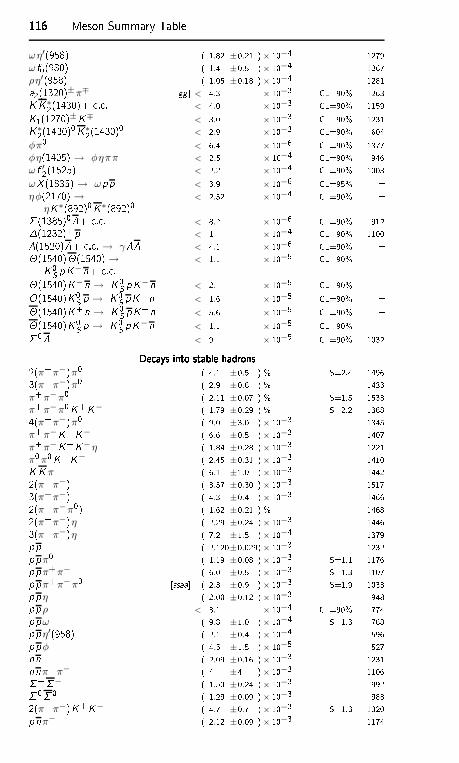
116116116116 Meson Summary Tableωη′(958) ( 1.82 ±0.21 )× 10−4 1279ω f0(980) ( 1.4 ±0.5 )× 10−4 1267ρη′(958) ( 1.05 ±0.18 )× 10−4 1281a2(1320)±π∓ [gg < 4.3 × 10⁻³ CL=90% 1263K K∗2(1430)+ . . < 4.0 × 10⁻³ CL=90% 1159K1(1270)±K∓ < 3.0 × 10⁻³ CL=90% 1231K∗2(1430)0K∗2(1430)0 < 2.9 × 10⁻³ CL=90% 604φπ0 < 6.4 × 10⁻⁶ CL=90% 1377φη(1405) → φηππ < 2.5 × 10⁻⁴ CL=90% 946ω f ′2(1525) < 2.2 × 10⁻⁴ CL=90% 1003ωX (1835) → ωpp < 3.9 × 10⁻⁶ CL=95% ηφ(2170) →
ηK∗(892)0K∗(892)0 < 2.52 × 10⁻⁴ CL=90% (1385)0+ . . < 8.2 × 10⁻⁶ CL=90% 912(1232)+p < 1 × 10⁻⁴ CL=90% 1100(1520)+ . . → γ < 4.1 × 10⁻⁶ CL=90% (1540)(1540) →K0S pK−n+ . . < 1.1 × 10⁻⁵ CL=90% (1540)K−n → K0S pK−n < 2.1 × 10⁻⁵ CL=90% (1540)K0S p → K0S pK+n < 1.6 × 10⁻⁵ CL=90% (1540)K+n → K0S pK+n < 5.6 × 10⁻⁵ CL=90% (1540)K0S p → K0S pK−n < 1.1 × 10⁻⁵ CL=90% 0 < 9 × 10⁻⁵ CL=90% 1032De ays into stable hadronsDe ays into stable hadronsDe ays into stable hadronsDe ays into stable hadrons2(π+π−)π0 ( 4.1 ±0.5 ) % S=2.4 14963(π+π−)π0 ( 2.9 ±0.6 ) % 1433π+π−π0 ( 2.11 ±0.07 ) % S=1.5 1533π+π−π0K+K− ( 1.79 ±0.29 ) % S=2.2 13684(π+π−)π0 ( 9.0 ±3.0 )× 10−3 1345π+π−K+K− ( 6.6 ±0.5 )× 10−3 1407π+π−K+K−η ( 1.84 ±0.28 )× 10−3 1221π0π0K+K− ( 2.45 ±0.31 )× 10−3 1410K K π ( 6.1 ±1.0 )× 10−3 14422(π+π−) ( 3.57 ±0.30 )× 10−3 15173(π+π−) ( 4.3 ±0.4 )× 10−3 14662(π+π−π0) ( 1.62 ±0.21 ) % 14682(π+π−)η ( 2.29 ±0.24 )× 10−3 14463(π+π−)η ( 7.2 ±1.5 )× 10−4 1379pp ( 2.120±0.029)× 10−3 1232ppπ0 ( 1.19 ±0.08 )× 10−3 S=1.1 1176ppπ+π− ( 6.0 ±0.5 )× 10−3 S=1.3 1107ppπ+π−π0 [ssaa ( 2.3 ±0.9 )× 10−3 S=1.9 1033ppη ( 2.00 ±0.12 )× 10−3 948ppρ < 3.1 × 10⁻⁴ CL=90% 774ppω ( 9.8 ±1.0 )× 10−4 S=1.3 768ppη′(958) ( 2.1 ±0.4 )× 10−4 596ppφ ( 4.5 ±1.5 )× 10−5 527nn ( 2.09 ±0.16 )× 10−3 1231nnπ+π− ( 4 ±4 )× 10−3 1106+− ( 1.50 ±0.24 )× 10−3 99200 ( 1.29 ±0.09 )× 10−3 9882(π+π−)K+K− ( 4.7 ±0.7 )× 10−3 S=1.3 1320pnπ− ( 2.12 ±0.09 )× 10−3 1174
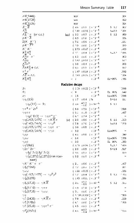
Meson Summary Table 117117117117nN(1440) seen 984nN(1520) seen 928nN(1535) seen 914−+ ( 8.6 ±1.1 )× 10−4 S=1.2 807 ( 1.61 ±0.15 )× 10−3 S=1.9 1074−π+ (or . .) [gg ( 8.3 ±0.7 )× 10−4 S=1.2 950pK− ( 8.9 ±1.6 )× 10−4 8762(K+K−) ( 7.6 ±0.9 )× 10−4 1131pK−0 ( 2.9 ±0.8 )× 10−4 819K+K− ( 2.70 ±0.17 )× 10−4 1468K0S K0L ( 2.1 ±0.4 )× 10−4 S=3.2 1466π+π− ( 4.3 ±1.0 )× 10−3 903η ( 1.62 ±0.17 )× 10−4 672π0 ( 3.8 ±0.4 )× 10−5 998nK0S + . . ( 6.5 ±1.1 )× 10−4 872π+π− ( 1.47 ±0.14 )× 10−4 1542+ . . ( 2.83 ±0.23 )× 10−5 1034K0S K0S < 1 × 10⁻⁶ CL=95% 1466Radiative de aysRadiative de aysRadiative de aysRadiative de ays3γ ( 1.16 ±0.22 )× 10−5 15484γ < 9 × 10⁻⁶ CL=90% 15485γ < 1.5 × 10⁻⁵ CL=90% 1548γ η (1S) ( 1.7 ±0.4 ) % S=1.6 111
γ η (1S) → 3γ ( 3.8 +1.3−1.0 )× 10−6 S=1.1
γπ+π−2π0 ( 8.3 ±3.1 )× 10−3 1518γ ηππ ( 6.1 ±1.0 )× 10−3 1487
γ η2(1870) → γ ηπ+π− ( 6.2 ±2.4 )× 10−4 γ η(1405/1475) → γK K π [o ( 2.8 ±0.6 )× 10−3 S=1.6 1223γ η(1405/1475) → γ γ ρ0 ( 7.8 ±2.0 )× 10−5 S=1.8 1223γ η(1405/1475) → γ ηπ+π− ( 3.0 ±0.5 )× 10−4 γ η(1405/1475) → γ γφ < 8.2 × 10⁻⁵ CL=95% γ ρρ ( 4.5 ±0.8 )× 10−3 1340γ ρω < 5.4 × 10⁻⁴ CL=90% 1338γ ρφ < 8.8 × 10⁻⁵ CL=90% 1258γ η′(958) ( 5.15 ±0.16 )× 10−3 S=1.2 1400γ 2π+2π− ( 2.8 ±0.5 )× 10−3 S=1.9 1517
γ f2(1270)f2(1270) ( 9.5 ±1.7 )× 10−4 879γ f2(1270)f2(1270)(non reso-nant) ( 8.2 ±1.9 )× 10−4
γK+K−π+π− ( 2.1 ±0.6 )× 10−3 1407γ f4(2050) ( 2.7 ±0.7 )× 10−3 891γωω ( 1.61 ±0.33 )× 10−3 1336γ η(1405/1475) → γ ρ0 ρ0 ( 1.7 ±0.4 )× 10−3 S=1.3 1223γ f2(1270) ( 1.43 ±0.11 )× 10−3 1286γ f0(1710) → γK K ( 8.5 +1.2
−0.9 )× 10−4 S=1.2 1075γ f0(1710) → γππ ( 4.0 ±1.0 )× 10−4 γ f0(1710) → γωω ( 3.1 ±1.0 )× 10−4 γ η ( 1.104±0.034)× 10−3 1500γ f1(1420) → γK K π ( 7.9 ±1.3 )× 10−4 1220γ f1(1285) ( 6.1 ±0.8 )× 10−4 1283γ f1(1510) → γ ηπ+π− ( 4.5 ±1.2 )× 10−4 γ f ′2(1525) ( 4.5 +0.7
−0.4 )× 10−4 1173
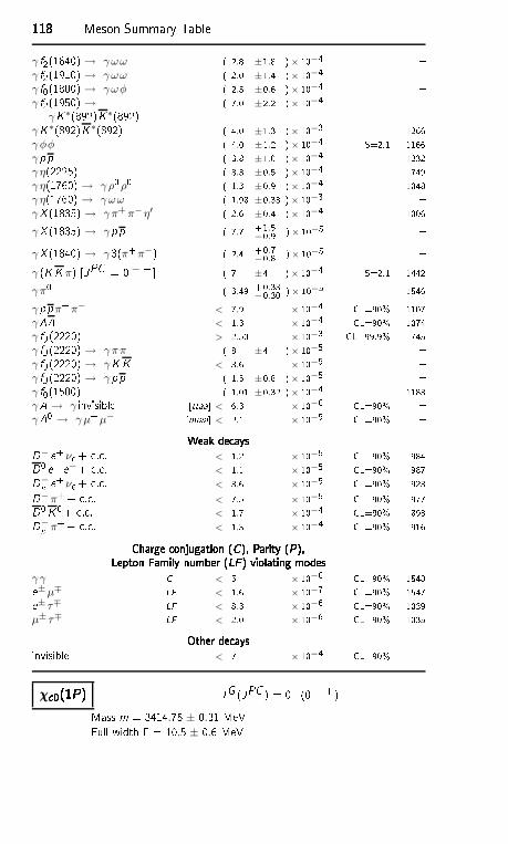
118118118118 Meson Summary Tableγ f2(1640) → γωω ( 2.8 ±1.8 )× 10−4 γ f2(1910) → γωω ( 2.0 ±1.4 )× 10−4 γ f0(1800) → γωφ ( 2.5 ±0.6 )× 10−4 γ f2(1950) →
γK∗(892)K∗(892) ( 7.0 ±2.2 )× 10−4 γK∗(892)K∗(892) ( 4.0 ±1.3 )× 10−3 1266γφφ ( 4.0 ±1.2 )× 10−4 S=2.1 1166γ pp ( 3.8 ±1.0 )× 10−4 1232γ η(2225) ( 3.3 ±0.5 )× 10−4 749γ η(1760) → γ ρ0ρ0 ( 1.3 ±0.9 )× 10−4 1048γ η(1760) → γωω ( 1.98 ±0.33 )× 10−3 γX (1835) → γπ+π−η′ ( 2.6 ±0.4 )× 10−4 1006γX (1835) → γ pp ( 7.7 +1.5
−0.9 )× 10−5 γX (1840) → γ 3(π+π−) ( 2.4 +0.7
−0.8 )× 10−5 γ (K K π) [JPC = 0−+ ( 7 ±4 )× 10−4 S=2.1 1442γπ0 ( 3.49 +0.33
−0.30 )× 10−5 1546γ ppπ+π− < 7.9 × 10⁻⁴ CL=90% 1107γ < 1.3 × 10⁻⁴ CL=90% 1074γ fJ (2220) > 2.50 × 10⁻³ CL=99.9% 745γ fJ (2220) → γππ ( 8 ±4 )× 10−5 γ fJ (2220) → γK K < 3.6 × 10⁻⁵ γ fJ (2220) → γ pp ( 1.5 ±0.8 )× 10−5 γ f0(1500) ( 1.01 ±0.32 )× 10−4 1183γA → γ invisible [ttaa < 6.3 × 10⁻⁶ CL=90% γA0 → γµ+µ− [uuaa < 2.1 × 10⁻⁵ CL=90% Weak de aysWeak de aysWeak de aysWeak de aysD− e+νe+ . . < 1.2 × 10⁻⁵ CL=90% 984D0 e+ e−+ . . < 1.1 × 10⁻⁵ CL=90% 987D−s e+νe+ . . < 3.6 × 10⁻⁵ CL=90% 923D−π++ . . < 7.5 × 10⁻⁵ CL=90% 977D0K0+ . . < 1.7 × 10⁻⁴ CL=90% 898D−s π++ . . < 1.3 × 10⁻⁴ CL=90% 916Charge onjugation (C ), Parity (P),Charge onjugation (C ), Parity (P),Charge onjugation (C ), Parity (P),Charge onjugation (C ), Parity (P),Lepton Family number (LF ) violating modesLepton Family number (LF ) violating modesLepton Family number (LF ) violating modesLepton Family number (LF ) violating modesγ γ C < 5 × 10⁻⁶ CL=90% 1548e±µ∓ LF < 1.6 × 10⁻⁷ CL=90% 1547e± τ∓ LF < 8.3 × 10⁻⁶ CL=90% 1039µ± τ∓ LF < 2.0 × 10⁻⁶ CL=90% 1035Other de aysOther de aysOther de aysOther de aysinvisible < 7 × 10⁻⁴ CL=90% χ 0(1P)χ 0(1P)χ 0(1P)χ 0(1P) IG (JPC ) = 0+(0 + +)Mass m = 3414.75 ± 0.31 MeVFull width = 10.5 ± 0.6 MeV
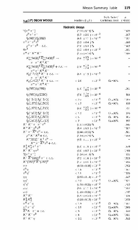
Meson Summary Table 119119119119S ale fa tor/ pχ 0(1P) DECAY MODESχ 0(1P) DECAY MODESχ 0(1P) DECAY MODESχ 0(1P) DECAY MODES Fra tion (i /) Conden e level (MeV/ )Hadroni de aysHadroni de aysHadroni de aysHadroni de ays2(π+π−) (2.24±0.18) % 1679
ρ0π+π− (8.7 ±2.8 )× 10−3 1607f0(980)f0(980) (6.5 ±2.1 )× 10−4 1391π+π−π0π0 (3.3 ±0.4 ) % 1680
ρ+π−π0+ . . (2.8 ±0.4 ) % 16074π0 (3.2 ±0.4 )× 10−3 1681π+π−K+K− (1.75±0.14) % 1580K∗0(1430)0K∗0(1430)0 →
π+π−K+K−(9.6 +3.5
−2.8 ) × 10−4 K∗0(1430)0K∗2(1430)0+ . . →π+π−K+K−
(7.8 +1.9−2.4 ) × 10−4 K1(1270)+K−+ . . →
π+π−K+K−(6.1 ±1.9 )× 10−3 K1(1400)+K−+ . . →
π+π−K+K−< 2.6 × 10⁻³ CL=90% f0(980)f0(980) (1.6 +1.0
−0.9 ) × 10−4 1391f0(980)f0(2200) (7.8 +2.0−2.5 ) × 10−4 584f0(1370)f0(1370) < 2.7 × 10⁻⁴ CL=90% 1019f0(1370)f0(1500) < 1.7 × 10⁻⁴ CL=90% 920f0(1370)f0(1710) (6.6 +3.5−2.3 ) × 10−4 721f0(1500)f0(1370) < 1.3 × 10⁻⁴ CL=90% 920f0(1500)f0(1500) < 5 × 10⁻⁵ CL=90% 805f0(1500)f0(1710) < 7 × 10⁻⁵ CL=90% 557K+K−π+π−π0 (1.11±0.26) % 1545K+K−π0π0 (5.4 ±0.9 )× 10−3 1582K+π−K0π0+ . . (2.44±0.33) % 1581
ρ+K−K0+ . . (1.18±0.21) % 1458K∗(892)−K+π0 →K+π−K0π0+ . . (4.5 ±1.1 )× 10−3 K0S K0S π+π− (5.6 ±1.0 )× 10−3 1579K+K−ηπ0 (3.0 ±0.7 )× 10−3 14683(π+π−) (1.20±0.18) % 1633K+K∗(892)0π−+ . . (7.2 ±1.6 )× 10−3 1523K∗(892)0K∗(892)0 (1.7 ±0.6 )× 10−3 1456ππ (8.33±0.35)× 10−3 1702π0 η < 1.8 × 10⁻⁴ 1661π0 η′ < 1.1 × 10⁻³ 1570ηη (2.95±0.19)× 10−3 1617ηη′ < 2.3 × 10⁻⁴ CL=90% 1521η′ η′ (1.96±0.21)× 10−3 1413ωω (9.5 ±1.1 )× 10−4 1517ωφ (1.16±0.21)× 10−4 1447K+K− (5.91±0.32)× 10−3 1634K0S K0S (3.10±0.18)× 10−3 1633π+π−η < 1.9 × 10⁻⁴ CL=90% 1651π+π−η′ < 3.5 × 10⁻⁴ CL=90% 1560K0K+π−+ . . < 9 × 10⁻⁵ CL=90% 1610K+K−π0 < 6 × 10⁻⁵ CL=90% 1611K+K−η < 2.2 × 10⁻⁴ CL=90% 1512
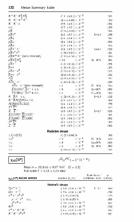
120120120120 Meson Summary TableK+K−K0S K0S (1.4 ±0.5 )× 10−3 1331K+K−K+K− (2.75±0.28)× 10−3 1333K+K−φ (9.5 ±2.4 )× 10−4 1381φφ (7.7 ±0.7 )× 10−4 1370pp (2.25±0.09)× 10−4 1426ppπ0 (6.8 ±0.7 )× 10−4 S=1.3 1379ppη (3.5 ±0.4 )× 10−4 1187ppω (5.1 ±0.6 )× 10−4 1043ppφ (5.9 ±1.4 )× 10−5 876ppπ+π− (2.1 ±0.7 )× 10−3 S=1.4 1320ppπ0π0 (1.02±0.27)× 10−3 1324ppK+K− (non-resonant) (1.19±0.26)× 10−4 890ppK0S K0S < 8.8 × 10⁻⁴ CL=90% 884pnπ− (1.24±0.11)× 10−3 1376pnπ+ (1.34±0.12)× 10−3 1376pnπ−π0 (2.29±0.21)× 10−3 1321pnπ+π0 (2.16±0.18)× 10−3 1321 (3.21±0.25)× 10−4 1292π+π− (1.15±0.13)× 10−3 1153π+π− (non-resonant) < 5 × 10⁻⁴ CL=90% 1153 (1385)+π−+ . . < 5 × 10⁻⁴ CL=90% 1083 (1385)−π++ . . < 5 × 10⁻⁴ CL=90% 1083K+p+ . . (1.22±0.12)× 10−3 S=1.3 1132K+p(1520)+ . . (2.9 ±0.7 )× 10−4 858(1520)(1520) (3.1 ±1.2 )× 10−4 77900 (4.4 ±0.4 )× 10−4 1222+− (3.9 ±0.7 )× 10−4 S=1.7 1225 (1385)+ (1385)− (1.6 ±0.6 )× 10−4 1001 (1385)− (1385)+ (2.3 ±0.6 )× 10−4 1001 0 0 (3.1 ±0.8 )× 10−4 1089−+ (4.7 ±0.7 )× 10−4 1081Radiative de aysRadiative de aysRadiative de aysRadiative de aysγ J/ψ(1S) (1.27±0.06) % 303γ ρ0 < 9 × 10⁻⁶ CL=90% 1619γω < 8 × 10⁻⁶ CL=90% 1618γφ < 6 × 10⁻⁶ CL=90% 1555γ γ (2.23±0.13)× 10−4 1707χ 1(1P)χ 1(1P)χ 1(1P)χ 1(1P) IG (JPC ) = 0+(1 + +)Mass m = 3510.66 ± 0.07 MeV (S = 1.5)Full width = 0.84 ± 0.04 MeV S ale fa tor/ p
χ 1(1P) DECAY MODESχ 1(1P) DECAY MODESχ 1(1P) DECAY MODESχ 1(1P) DECAY MODES Fra tion (i /) Conden e level (MeV/ )Hadroni de aysHadroni de aysHadroni de aysHadroni de ays3(π+π−) ( 5.8 ±1.4 )× 10−3 S=1.2 16832(π+π−) ( 7.6 ±2.6 )× 10−3 1728π+π−π0π0 ( 1.22±0.16) % 1729
ρ+π−π0+ . . ( 1.48±0.25) % 1658ρ0π+π− ( 3.9 ±3.5 )× 10−3 16574π0 ( 5.5 ±0.8 )× 10−4 1729
π+π−K+K− ( 4.5 ±1.0 )× 10−3 1632K+K−π0π0 ( 1.14±0.28)× 10−3 1634
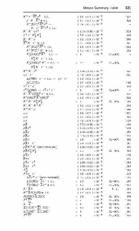
Meson Summary Table 121121121121K+π−K0π0+ . . ( 8.7 ±1.4 )× 10−3 1632ρ−K+K0+ . . ( 5.1 ±1.2 )× 10−3 1514K∗(892)0K0π0 →K+π−K0π0+ . . ( 2.4 ±0.7 )× 10−3 K+K−ηπ0 ( 1.14±0.35)× 10−3 1523
π+π−K0S K0S ( 7.0 ±3.0 )× 10−4 1630K+K−η ( 3.2 ±1.0 )× 10−4 1566K0K+π−+ . . ( 7.1 ±0.6 )× 10−3 1661K∗(892)0K0+ . . ( 1.0 ±0.4 )× 10−3 1602K∗(892)+K−+ . . ( 1.5 ±0.7 )× 10−3 1602K∗J (1430)0K0+ . . →K0S K+π−+ . . < 8 × 10⁻⁴ CL=90% K∗J (1430)+K−+ . . →K0S K+π−+ . . < 2.2 × 10⁻³ CL=90% K+K−π0 ( 1.85±0.25)× 10−3 1662ηπ+π− ( 4.9 ±0.5 )× 10−3 1701a0(980)+π−+ . . → ηπ+π− ( 1.8 ±0.6 )× 10−3 f2(1270)η ( 2.7 ±0.8 )× 10−3 1468π+π−η′ ( 2.3 ±0.5 )× 10−3 1612π0 f0(980) → π0π+π− < 6 × 10⁻⁶ CL=90% K+K∗(892)0π−+ . . ( 3.2 ±2.1 )× 10−3 1577K∗(892)0K∗(892)0 ( 1.5 ±0.4 )× 10−3 1512K+K−K0S K0S < 4 × 10⁻⁴ CL=90% 1390K+K−K+K− ( 5.5 ±1.1 )× 10−4 1393K+K−φ ( 4.2 ±1.6 )× 10−4 1440ωω ( 5.8 ±0.7 )× 10−4 1571ωφ ( 2.1 ±0.6 )× 10−5 1503φφ ( 4.2 ±0.5 )× 10−4 1429pp ( 7.72±0.35)× 10−5 1484ppπ0 ( 1.59±0.19)× 10−4 1438ppη ( 1.48±0.25)× 10−4 1254ppω ( 2.16±0.31)× 10−4 1117ppφ < 1.8 × 10⁻⁵ CL=90% 962ppπ+π− ( 5.0 ±1.9 )× 10−4 1381ppK+K− (non-resonant) ( 1.30±0.23)× 10−4 974ppK0S K0S < 4.5 × 10⁻⁴ CL=90% 968pnπ− ( 3.9 ±0.5 )× 10−4 1435pnπ+ ( 4.0 ±0.5 )× 10−4 1435pnπ−π0 ( 1.05±0.12)× 10−3 1383pnπ+π0 ( 1.03±0.12)× 10−3 1383 ( 1.16±0.12)× 10−4 1355π+π− ( 3.0 ±0.5 )× 10−4 1223π+π− (non-resonant) ( 2.5 ±0.6 )× 10−4 1223 (1385)+π−+ . . < 1.3 × 10⁻⁴ CL=90% 1157 (1385)−π++ . . < 1.3 × 10⁻⁴ CL=90% 1157K+p ( 4.2 ±0.4 )× 10−4 S=1.1 1203K+p(1520)+ . . ( 1.7 ±0.5 )× 10−4 950(1520)(1520) < 1.0 × 10⁻⁴ CL=90% 87900 < 4 × 10⁻⁵ CL=90% 1288+− < 6 × 10⁻⁵ CL=90% 1291 (1385)+ (1385)− < 1.0 × 10⁻⁴ CL=90% 1081 (1385)− (1385)+ < 5 × 10⁻⁵ CL=90% 1081 0 0 < 6 × 10⁻⁵ CL=90% 1163
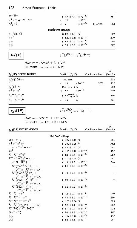
122122122122 Meson Summary Table−+ ( 8.2 ±2.2 )× 10−5 1155π+π− + K+K− < 2.1 × 10⁻³ K0S K0S < 6 × 10⁻⁵ CL=90% 1683Radiative de aysRadiative de aysRadiative de aysRadiative de aysγ J/ψ(1S) (33.9 ±1.2 ) % 389γ ρ0 ( 2.20±0.18)× 10−4 1670γω ( 6.9 ±0.8 )× 10−5 1668γφ ( 2.5 ±0.5 )× 10−5 1607h (1P)h (1P)h (1P)h (1P) IG (JPC ) = ??(1 +−)Mass m = 3525.38 ± 0.11 MeVFull width = 0.7 ± 0.4 MeV ph (1P) DECAY MODESh (1P) DECAY MODESh (1P) DECAY MODESh (1P) DECAY MODES Fra tion (i /) Conden e level (MeV/ )J/ψ(1S)ππ not seen 312pp < 1.5 × 10⁻⁴ 90% 1492η (1S)γ (51 ±6 ) % 500π+π−π0 < 2.2 × 10⁻³ 17492π+2π−π0 ( 2.2+0.8
−0.7) % 17163π+3π−π0 < 2.9 % 1661χ 2(1P)χ 2(1P)χ 2(1P)χ 2(1P) IG (JPC ) = 0+(2 + +)Mass m = 3556.20 ± 0.09 MeVFull width = 1.93 ± 0.11 MeV p
χ 2(1P) DECAY MODESχ 2(1P) DECAY MODESχ 2(1P) DECAY MODESχ 2(1P) DECAY MODES Fra tion (i /) Conden e level (MeV/ )Hadroni de aysHadroni de aysHadroni de aysHadroni de ays2(π+π−) ( 1.07±0.10) % 1751π+π−π0π0 ( 1.92±0.25) % 1752
ρ+π−π0+ . . ( 2.3 ±0.4 ) % 16824π0 ( 1.16±0.16)× 10−3 1752K+K−π0π0 ( 2.2 ±0.4 )× 10−3 1658K+π−K0π0+ . . ( 1.44±0.21) % 1657ρ−K+K0+ . . ( 4.3 ±1.3 )× 10−3 1540K∗(892)0K−π+ →K−π+K0π0+ . . ( 3.1 ±0.8 )× 10−3 K∗(892)0K0π0 →K+π−K0π0+ . . ( 4.0 ±0.9 )× 10−3 K∗(892)−K+π0 →K+π−K0π0+ . . ( 3.9 ±0.9 )× 10−3 K∗(892)+K0π− →K+π−K0π0+ . . ( 3.1 ±0.8 )× 10−3 K+K−ηπ0 ( 1.3 ±0.5 )× 10−3 1549K+K−π+π− ( 8.8 ±1.0 )× 10−3 1656K+K−π+π−π0 ( 1.23±0.34) % 1623K+K∗(892)0π−+ . . ( 2.2 ±1.1 )× 10−3 1602K∗(892)0K∗(892)0 ( 2.4 ±0.5 )× 10−3 15383(π+π−) ( 8.6 ±1.8 )× 10−3 1707
φφ ( 1.12±0.10)× 10−3 1457ωω ( 8.8 ±1.1 )× 10−4 1597
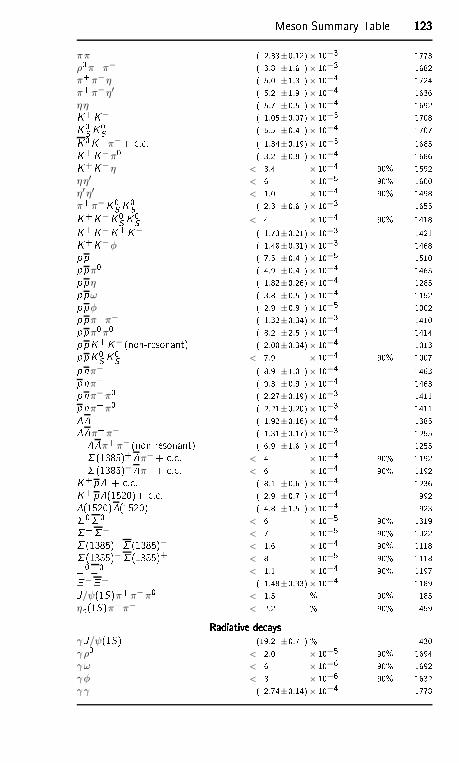
Meson Summary Table 123123123123ππ ( 2.33±0.12)× 10−3 1773ρ0π+π− ( 3.8 ±1.6 )× 10−3 1682π+π−η ( 5.0 ±1.3 )× 10−4 1724π+π−η′ ( 5.2 ±1.9 )× 10−4 1636ηη ( 5.7 ±0.5 )× 10−4 1692K+K− ( 1.05±0.07)× 10−3 1708K0S K0S ( 5.5 ±0.4 )× 10−4 1707K0K+π−+ . . ( 1.34±0.19)× 10−3 1685K+K−π0 ( 3.2 ±0.8 )× 10−4 1686K+K−η < 3.4 × 10⁻⁴ 90% 1592ηη′ < 6 × 10⁻⁵ 90% 1600η′ η′ < 1.0 × 10⁻⁴ 90% 1498π+π−K0S K0S ( 2.3 ±0.6 )× 10−3 1655K+K−K0S K0S < 4 × 10⁻⁴ 90% 1418K+K−K+K− ( 1.73±0.21)× 10−3 1421K+K−φ ( 1.48±0.31)× 10−3 1468pp ( 7.5 ±0.4 )× 10−5 1510ppπ0 ( 4.9 ±0.4 )× 10−4 1465ppη ( 1.82±0.26)× 10−4 1285ppω ( 3.8 ±0.5 )× 10−4 1152ppφ ( 2.9 ±0.9 )× 10−5 1002ppπ+π− ( 1.32±0.34)× 10−3 1410ppπ0π0 ( 8.2 ±2.5 )× 10−4 1414ppK+K− (non-resonant) ( 2.00±0.34)× 10−4 1013ppK0S K0S < 7.9 × 10⁻⁴ 90% 1007pnπ− ( 8.9 ±1.0 )× 10−4 1463pnπ+ ( 9.3 ±0.9 )× 10−4 1463pnπ−π0 ( 2.27±0.19)× 10−3 1411pnπ+π0 ( 2.21±0.20)× 10−3 1411 ( 1.92±0.16)× 10−4 1385π+π− ( 1.31±0.17)× 10−3 1255π+π− (non-resonant) ( 6.9 ±1.6 )× 10−4 1255 (1385)+π−+ . . < 4 × 10⁻⁴ 90% 1192 (1385)−π++ . . < 6 × 10⁻⁴ 90% 1192K+p + . . ( 8.1 ±0.6 )× 10−4 1236K+p(1520)+ . . ( 2.9 ±0.7 )× 10−4 992(1520)(1520) ( 4.8 ±1.5 )× 10−4 92300 < 6 × 10⁻⁵ 90% 1319+− < 7 × 10⁻⁵ 90% 1322 (1385)+ (1385)− < 1.6 × 10⁻⁴ 90% 1118 (1385)− (1385)+ < 8 × 10⁻⁵ 90% 1118 0 0 < 1.1 × 10⁻⁴ 90% 1197−+ ( 1.48±0.33)× 10−4 1189J/ψ(1S)π+π−π0 < 1.5 % 90% 185η (1S)π+π− < 2.2 % 90% 459Radiative de aysRadiative de aysRadiative de aysRadiative de aysγ J/ψ(1S) (19.2 ±0.7 ) % 430γ ρ0 < 2.0 × 10⁻⁵ 90% 1694γω < 6 × 10⁻⁶ 90% 1692γφ < 8 × 10⁻⁶ 90% 1632γ γ ( 2.74±0.14)× 10−4 1778
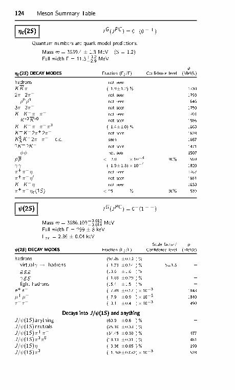
124124124124 Meson Summary Tableη (2S)η (2S)η (2S)η (2S) IG (JPC ) = 0+(0−+)Quantum numbers are quark model predi tions.Mass m = 3639.4 ± 1.3 MeV (S = 1.2)Full width = 11.3+3.2
−2.9 MeV pη (2S) DECAY MODESη (2S) DECAY MODESη (2S) DECAY MODESη (2S) DECAY MODES Fra tion (i /) Conden e level (MeV/ )hadrons not seen K K π ( 1.9±1.2) % 17302π+2π− not seen 1793
ρ0 ρ0 not seen 16463π+3π− not seen 1750K+K−π+π− not seen 1701K∗0K∗0 not seen 1586K+K−π+π−π0 ( 1.4±1.0) % 1668K+K−2π+2π− not seen 1628K0S K−2π+π−+ . . seen 16672K+2K− not seen 1471φφ not seen 1507pp < 2.0 × 10⁻³ 90% 1559
γ γ ( 1.9±1.3)× 10−4 1820π+π−η not seen 1767π+π−η′ not seen 1681K+K−η not seen 1638π+π−η (1S) < 25 % 90% 539ψ(2S)ψ(2S)ψ(2S)ψ(2S) IG (JPC ) = 0−(1−−)Mass m = 3686.109+0.012
−0.014 MeVFull width = 299 ± 8 keVe e = 2.36 ± 0.04 keV S ale fa tor/ pψ(2S) DECAY MODESψ(2S) DECAY MODESψ(2S) DECAY MODESψ(2S) DECAY MODES Fra tion (i /) Conden e level (MeV/ )hadrons (97.85 ±0.13 ) % virtualγ → hadrons ( 1.73 ±0.14 ) % S=1.5 g g g (10.6 ±1.6 ) %
γ g g ( 1.03 ±0.29 ) % light hadrons (15.4 ±1.5 ) % e+ e− ( 7.89 ±0.17 )× 10−3 1843µ+µ− ( 7.9 ±0.9 )× 10−3 1840τ+ τ− ( 3.1 ±0.4 )× 10−3 490De ays into J/ψ(1S) and anythingDe ays into J/ψ(1S) and anythingDe ays into J/ψ(1S) and anythingDe ays into J/ψ(1S) and anythingJ/ψ(1S)anything (60.9 ±0.6 ) % J/ψ(1S)neutrals (25.10 ±0.33 ) % J/ψ(1S)π+π− (34.45 ±0.30 ) % 477J/ψ(1S)π0π0 (18.13 ±0.31 ) % 481J/ψ(1S)η ( 3.36 ±0.05 ) % 199J/ψ(1S)π0 ( 1.268±0.032)× 10−3 528
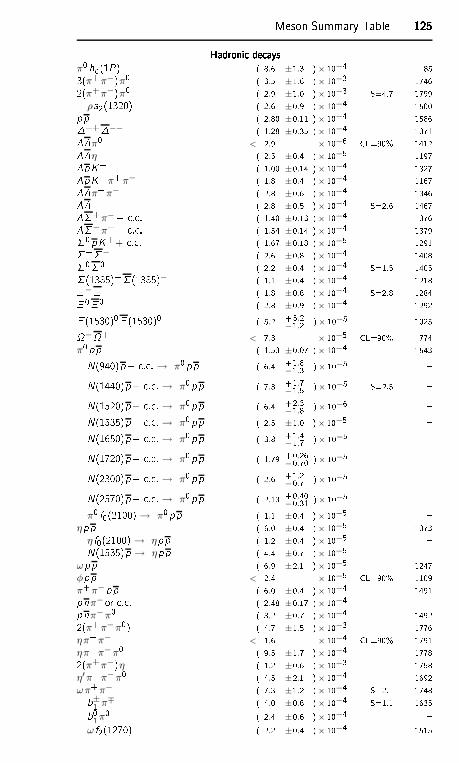
Meson Summary Table 125125125125Hadroni de aysHadroni de aysHadroni de aysHadroni de aysπ0 h (1P) ( 8.6 ±1.3 )× 10−4 853(π+π−)π0 ( 3.5 ±1.6 )× 10−3 17462(π+π−)π0 ( 2.9 ±1.0 )× 10−3 S=4.7 1799
ρa2(1320) ( 2.6 ±0.9 )× 10−4 1500pp ( 2.80 ±0.11 )× 10−4 1586++−− ( 1.28 ±0.35 )× 10−4 1371π0 < 2.9 × 10⁻⁶ CL=90% 1412η ( 2.5 ±0.4 )× 10−5 1197pK+ ( 1.00 ±0.14 )× 10−4 1327pK+π+π− ( 1.8 ±0.4 )× 10−4 1167π+π− ( 2.8 ±0.6 )× 10−4 1346 ( 2.8 ±0.5 )× 10−4 S=2.6 1467+π−+ . . ( 1.40 ±0.13 )× 10−4 1376−π++ . . ( 1.54 ±0.14 )× 10−4 13790 pK++ . . ( 1.67 ±0.18 )× 10−5 1291+− ( 2.6 ±0.8 )× 10−4 140800 ( 2.2 ±0.4 )× 10−4 S=1.5 1405 (1385)+ (1385)− ( 1.1 ±0.4 )× 10−4 1218−+ ( 1.8 ±0.6 )× 10−4 S=2.8 1284 0 0 ( 2.8 ±0.9 )× 10−4 1292 (1530)0 (1530)0 ( 5.2 +3.2−1.2 )× 10−5 1025−+ < 7.3 × 10⁻⁵ CL=90% 774
π0 pp ( 1.53 ±0.07 )× 10−4 1543N(940)p+ . . → π0 pp ( 6.4 +1.8−1.3 )× 10−5 N(1440)p+ . . → π0 pp ( 7.3 +1.7−1.5 )× 10−5 S=2.5 N(1520)p+ . . → π0 pp ( 6.4 +2.3−1.8 )× 10−6 N(1535)p+ . . → π0 pp ( 2.5 ±1.0 )× 10−5 N(1650)p+ . . → π0 pp ( 3.8 +1.4−1.7 )× 10−5 N(1720)p+ . . → π0 pp ( 1.79 +0.26−0.70 )× 10−5 N(2300)p+ . . → π0 pp ( 2.6 +1.2−0.7 )× 10−5 N(2570)p+ . . → π0 pp ( 2.13 +0.40−0.31 )× 10−5
π0 f0(2100) → π0 pp ( 1.1 ±0.4 )× 10−5 ηpp ( 6.0 ±0.4 )× 10−5 1373
η f0(2100) → ηpp ( 1.2 ±0.4 )× 10−5 N(1535)p → ηpp ( 4.4 ±0.7 )× 10−5 ωpp ( 6.9 ±2.1 )× 10−5 1247φpp < 2.4 × 10⁻⁵ CL=90% 1109π+π−pp ( 6.0 ±0.4 )× 10−4 1491pnπ− or . . ( 2.48 ±0.17 )× 10−4 pnπ−π0 ( 3.2 ±0.7 )× 10−4 14922(π+π−π0) ( 4.7 ±1.5 )× 10−3 1776ηπ+π− < 1.6 × 10⁻⁴ CL=90% 1791ηπ+π−π0 ( 9.5 ±1.7 )× 10−4 17782(π+π−)η ( 1.2 ±0.6 )× 10−3 1758η′π+π−π0 ( 4.5 ±2.1 )× 10−4 1692ωπ+π− ( 7.3 ±1.2 )× 10−4 S=2.1 1748b±1 π∓ ( 4.0 ±0.6 )× 10−4 S=1.1 1635b01π0 ( 2.4 ±0.6 )× 10−4
ω f2(1270) ( 2.2 ±0.4 )× 10−4 1515
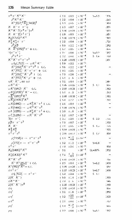
126126126126 Meson Summary Tableπ+π−K+K− ( 7.5 ±0.9 )× 10−4 S=1.9 1726
ρ0K+K− ( 2.2 ±0.4 )× 10−4 1616K∗(892)0K∗2(1430)0 ( 1.9 ±0.5 )× 10−4 1418K+K−π+π−η ( 1.3 ±0.7 )× 10−3 1574K+K−2(π+π−)π0 ( 1.00 ±0.31 )× 10−3 1611K+K−2(π+π−) ( 1.9 ±0.9 )× 10−3 1654K1(1270)±K∓ ( 1.00 ±0.28 )× 10−3 1581K0S K0S π+π− ( 2.2 ±0.4 )× 10−4 1724ρ0 pp ( 5.0 ±2.2 )× 10−5 1252K+K∗(892)0π−+ . . ( 6.7 ±2.5 )× 10−4 16742(π+π−) ( 2.4 ±0.6 )× 10−4 S=2.2 1817ρ0π+π− ( 2.2 ±0.6 )× 10−4 S=1.4 1750K+K−π+π−π0 ( 1.26 ±0.09 )× 10−3 1694ω f0(1710) → ωK+K− ( 5.9 ±2.2 )× 10−5 K∗(892)0K−π+π0 + . . ( 8.6 ±2.2 )× 10−4 K∗(892)+K−π+π− + . . ( 9.6 ±2.8 )× 10−4 K∗(892)+K−ρ0 + . . ( 7.3 ±2.6 )× 10−4 K∗(892)0K−ρ+ + . . ( 6.1 ±1.8 )× 10−4
ηK+K− , no ηφ ( 3.1 ±0.4 )× 10−5 1664ωK+K− ( 1.85 ±0.25 )× 10−4 S=1.1 1614ωK∗(892)+K−+ . . ( 2.07 ±0.26 )× 10−4 1482ωK∗2(1430)+K−+ . . ( 6.1 ±1.2 )× 10−5 1253ωK∗(892)0K0 ( 1.68 ±0.30 )× 10−4 1481ωK∗2(1430)0K0 ( 5.8 ±2.2 )× 10−5 1251ωX (1440) → ωK0S K−π++ . . ( 1.6 ±0.4 )× 10−5 ωX (1440) → ωK+K−π0 ( 1.09 ±0.26 )× 10−5 ω f1(1285) → ωK0S K−π++ . . ( 3.0 ±1.0 )× 10−6 ω f1(1285) → ωK+K−π0 ( 1.2 ±0.7 )× 10−6 3(π+π−) ( 3.5 ±2.0 )× 10−4 S=2.8 1774ppπ+π−π0 ( 7.3 ±0.7 )× 10−4 1435K+K− ( 7.1 ±0.5 )× 10−5 S=1.5 1776K0S K0L ( 5.34 ±0.33 )× 10−5 1775π+π−π0 ( 2.01 ±0.17 )× 10−4 S=1.7 1830
ρ(2150)π → π+π−π0 ( 1.9 +1.2−0.4 )× 10−4
ρ(770)π → π+π−π0 ( 3.2 ±1.2 )× 10−5 S=1.8 π+π− ( 7.8 ±2.6 )× 10−6 1838K1(1400)±K∓ < 3.1 × 10⁻⁴ CL=90% 1532K∗2(1430)±K∓ ( 7.1 +1.3
−0.9 )× 10−5 K+K−π0 ( 4.07 ±0.31 )× 10−5 1754K+K∗(892)−+ . . ( 2.9 ±0.4 )× 10−5 S=1.2 1698K∗(892)0K0+ . . ( 1.09 ±0.20 )× 10−4 1697φπ+π− ( 1.17 ±0.29 )× 10−4 S=1.7 1690
φ f0(980) → π+π− ( 6.8 ±2.4 )× 10−5 S=1.1 2(K+K−) ( 6.0 ±1.4 )× 10−5 1499φK+K− ( 7.0 ±1.6 )× 10−5 15462(K+K−)π0 ( 1.10 ±0.28 )× 10−4 1440φη ( 3.10 ±0.31 )× 10−5 1654φη′ ( 3.1 ±1.6 )× 10−5 1555ωη′ ( 3.2 +2.5
−2.1 )× 10−5 1623ωπ0 ( 2.1 ±0.6 )× 10−5 1757ρη′ ( 1.9 +1.7
−1.2 )× 10−5 1625ρη ( 2.2 ±0.6 )× 10−5 S=1.1 1717
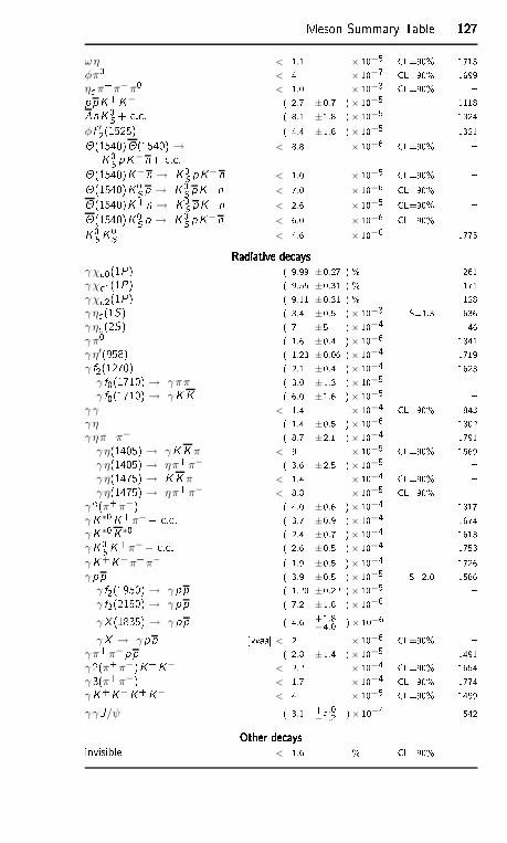
Meson Summary Table 127127127127ωη < 1.1 × 10⁻⁵ CL=90% 1715φπ0 < 4 × 10⁻⁷ CL=90% 1699η π+π−π0 < 1.0 × 10⁻³ CL=90% ppK+K− ( 2.7 ±0.7 )× 10−5 1118nK0S + . . ( 8.1 ±1.8 )× 10−5 1324φ f ′2(1525) ( 4.4 ±1.6 )× 10−5 1321(1540)(1540) →K0S pK−n+ . . < 8.8 × 10⁻⁶ CL=90% (1540)K−n → K0S pK−n < 1.0 × 10⁻⁵ CL=90% (1540)K0S p → K0S pK+n < 7.0 × 10⁻⁶ CL=90% (1540)K+n → K0S pK+n < 2.6 × 10⁻⁵ CL=90% (1540)K0S p → K0S pK−n < 6.0 × 10⁻⁶ CL=90% K0S K0S < 4.6 × 10⁻⁶ 1775Radiative de aysRadiative de aysRadiative de aysRadiative de aysγχ 0(1P) ( 9.99 ±0.27 ) % 261γχ 1(1P) ( 9.55 ±0.31 ) % 171γχ 2(1P) ( 9.11 ±0.31 ) % 128γ η (1S) ( 3.4 ±0.5 )× 10−3 S=1.3 636γ η (2S) ( 7 ±5 )× 10−4 46γπ0 ( 1.6 ±0.4 )× 10−6 1841γ η′(958) ( 1.23 ±0.06 )× 10−4 1719γ f2(1270) ( 2.1 ±0.4 )× 10−4 1623
γ f0(1710) → γππ ( 3.0 ±1.3 )× 10−5 γ f0(1710) → γK K ( 6.0 ±1.6 )× 10−5
γ γ < 1.4 × 10⁻⁴ CL=90% 1843γ η ( 1.4 ±0.5 )× 10−6 1802γ ηπ+π− ( 8.7 ±2.1 )× 10−4 1791
γ η(1405) → γK K π < 9 × 10⁻⁵ CL=90% 1569γ η(1405) → ηπ+π− ( 3.6 ±2.5 )× 10−5 γ η(1475) → K K π < 1.4 × 10⁻⁴ CL=90% γ η(1475) → ηπ+π− < 8.8 × 10⁻⁵ CL=90%
γ 2(π+π−) ( 4.0 ±0.6 )× 10−4 1817γK∗0K+π−+ . . ( 3.7 ±0.9 )× 10−4 1674γK∗0K∗0 ( 2.4 ±0.7 )× 10−4 1613γK0S K+π−+ . . ( 2.6 ±0.5 )× 10−4 1753γK+K−π+π− ( 1.9 ±0.5 )× 10−4 1726γ pp ( 3.9 ±0.5 )× 10−5 S=2.0 1586
γ f2(1950) → γ pp ( 1.20 ±0.22 )× 10−5 γ f2(2150) → γ pp ( 7.2 ±1.8 )× 10−6 γX (1835) → γ pp ( 4.6 +1.8
−4.0 )× 10−6 γX → γ pp [vvaa < 2 × 10⁻⁶ CL=90%
γπ+π−pp ( 2.8 ±1.4 )× 10−5 1491γ 2(π+π−)K+K− < 2.2 × 10⁻⁴ CL=90% 1654γ 3(π+π−) < 1.7 × 10⁻⁴ CL=90% 1774γK+K−K+K− < 4 × 10⁻⁵ CL=90% 1499γ γ J/ψ ( 3.1 +1.0
−1.2 )× 10−4 542Other de aysOther de aysOther de aysOther de aysinvisible < 1.6 % CL=90%
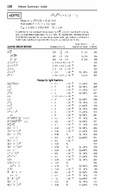
128128128128 Meson Summary Tableψ(3770)ψ(3770)ψ(3770)ψ(3770) IG (JPC ) = 0−(1−−)Mass m = 3773.15 ± 0.33 MeVFull width = 27.2 ± 1.0 MeVee = 0.262 ± 0.018 keV (S = 1.4)In addition to the dominant de ay mode to DD, ψ(3770) was found to de ayinto the nal states ontaining the J/ψ (BAI 05, ADAM 06). ADAMS 06 andHUANG 06A sear hed for various de ay modes with light hadrons and found astatisti ally signi ant signal for the de ay to φη only (ADAMS 06).S ale fa tor/ p
ψ(3770) DECAY MODESψ(3770) DECAY MODESψ(3770) DECAY MODESψ(3770) DECAY MODES Fra tion (i /) Conden e level (MeV/ )DD (93 +8−9 ) % S=2.0 286D0D0 (52 ±5 ) % S=2.0 286D+D− (41 ±4 ) % S=2.0 252J/ψπ+π− ( 1.93±0.28)× 10−3 560J/ψπ0π0 ( 8.0 ±3.0 )× 10−4 564J/ψη ( 9 ±4 )× 10−4 360J/ψπ0 < 2.8 × 10⁻⁴ CL=90% 603e+ e− ( 9.6 ±0.7 )× 10−6 S=1.3 1887De ays to light hadronsDe ays to light hadronsDe ays to light hadronsDe ays to light hadronsb1(1235)π < 1.4 × 10⁻⁵ CL=90% 1683
φη′ < 7 × 10⁻⁴ CL=90% 1607ωη′ < 4 × 10⁻⁴ CL=90% 1672ρ0 η′ < 6 × 10⁻⁴ CL=90% 1674φη ( 3.1 ±0.7 )× 10−4 1703ωη < 1.4 × 10⁻⁵ CL=90% 1762ρ0 η < 5 × 10⁻⁴ CL=90% 1764φπ0 < 3 × 10⁻⁵ CL=90% 1746ωπ0 < 6 × 10⁻⁴ CL=90% 1803π+π−π0 < 5 × 10⁻⁶ CL=90% 1874
ρπ < 5 × 10⁻⁶ CL=90% 1804K∗(892)+K−+ . . < 1.4 × 10⁻⁵ CL=90% 1745K∗(892)0K0+ . . < 1.2 × 10⁻³ CL=90% 1744K0S K0L < 1.2 × 10⁻⁵ CL=90% 18202(π+π−) < 1.12 × 10⁻³ CL=90% 18612(π+π−)π0 < 1.06 × 10⁻³ CL=90% 18432(π+π−π0) < 5.85 % CL=90% 1821ωπ+π− < 6.0 × 10⁻⁴ CL=90% 17943(π+π−) < 9.1 × 10⁻³ 18193(π+π−)π0 < 1.37 % 17923(π+π−)2π0 < 11.74 % CL=90% 1760
ηπ+π− < 1.24 × 10⁻³ CL=90% 1836π+π−2π0 < 8.9 × 10⁻³ CL=90% 1862ρ0π+π− < 6.9 × 10⁻³ CL=90% 1796η3π < 1.34 × 10⁻³ CL=90% 1824η2(π+π−) < 2.43 % 1804
ηρ0π+π− < 1.45 % CL=90% 1708η′ 3π < 2.44 × 10⁻³ CL=90% 1740K+K−π+π− < 9.0 × 10⁻⁴ CL=90% 1772
φπ+π− < 4.1 × 10⁻⁴ CL=90% 1737K+K−2π0 < 4.2 × 10⁻³ CL=90% 17744(π+π−) < 1.67 % CL=90% 17574(π+π−)π0 < 3.06 % CL=90% 1720
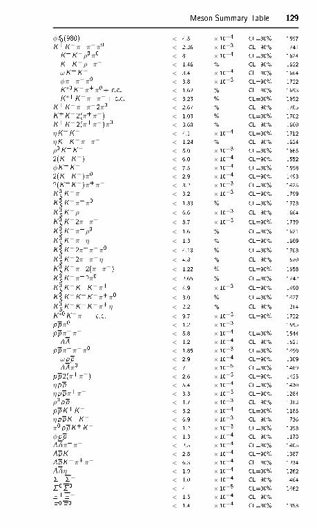
Meson Summary Table 129129129129φ f0(980) < 4.5 × 10⁻⁴ CL=90% 1597K+K−π+π−π0 < 2.36 × 10⁻³ CL=90% 1741K+K−ρ0π0 < 8 × 10⁻⁴ CL=90% 1624K+K−ρ+π− < 1.46 % CL=90% 1622
ωK+K− < 3.4 × 10⁻⁴ CL=90% 1664φπ+π−π0 < 3.8 × 10⁻³ CL=90% 1722K∗0K−π+π0+ . . < 1.62 % CL=90% 1693K∗+K−π+π−+ . . < 3.23 % CL=90% 1692K+K−π+π−2π0 < 2.67 % CL=90% 1705K+K−2(π+π−) < 1.03 % CL=90% 1702K+K−2(π+π−)π0 < 3.60 % CL=90% 1660
ηK+K− < 4.1 × 10⁻⁴ CL=90% 1712ηK+K−π+π− < 1.24 % CL=90% 1624ρ0K+K− < 5.0 × 10⁻³ CL=90% 16652(K+K−) < 6.0 × 10⁻⁴ CL=90% 1552φK+K− < 7.5 × 10⁻⁴ CL=90% 15982(K+K−)π0 < 2.9 × 10⁻⁴ CL=90% 14932(K+K−)π+π− < 3.2 × 10⁻³ CL=90% 1425K0S K−π+ < 3.2 × 10⁻³ CL=90% 1799K0S K−π+π0 < 1.33 % CL=90% 1773K0S K−ρ+ < 6.6 × 10⁻³ CL=90% 1664K0S K−2π+π− < 8.7 × 10⁻³ CL=90% 1739K0S K−π+ ρ0 < 1.6 % CL=90% 1621K0S K−π+ η < 1.3 % CL=90% 1669K0S K−2π+π−π0 < 4.18 % CL=90% 1703K0S K−2π+π− η < 4.8 % CL=90% 1570K0S K−π+ 2(π+π−) < 1.22 % CL=90% 1658K0S K−π+ 2π0 < 2.65 % CL=90% 1742K0S K−K+K−π+ < 4.9 × 10⁻³ CL=90% 1490K0S K−K+K−π+π0 < 3.0 % CL=90% 1427K0S K−K+K−π+ η < 2.2 % CL=90% 1214K∗0K−π++ . . < 9.7 × 10⁻³ CL=90% 1722ppπ0 < 1.2 × 10⁻³ 1595ppπ+π− < 5.8 × 10⁻⁴ CL=90% 1544 < 1.2 × 10⁻⁴ CL=90% 1521ppπ+π−π0 < 1.85 × 10⁻³ CL=90% 1490
ωpp < 2.9 × 10⁻⁴ CL=90% 1309π0 < 7 × 10⁻⁵ CL=90% 1469pp2(π+π−) < 2.6 × 10⁻³ CL=90% 1425ηpp < 5.4 × 10⁻⁴ CL=90% 1430ηppπ+π− < 3.3 × 10⁻³ CL=90% 1284ρ0 pp < 1.7 × 10⁻³ CL=90% 1313ppK+K− < 3.2 × 10⁻⁴ CL=90% 1185ηppK+K− < 6.9 × 10⁻³ CL=90% 736π0 ppK+K− < 1.2 × 10⁻³ CL=90% 1093φpp < 1.3 × 10⁻⁴ CL=90% 1178π+π− < 2.5 × 10⁻⁴ CL=90% 1405pK+ < 2.8 × 10⁻⁴ CL=90% 1387pK+π+π− < 6.3 × 10⁻⁴ CL=90% 1234η < 1.9 × 10⁻⁴ CL=90% 1262+− < 1.0 × 10⁻⁴ CL=90% 146400 < 4 × 10⁻⁵ CL=90% 1462+− < 1.5 × 10⁻⁴ CL=90% 0 0 < 1.4 × 10⁻⁴ CL=90% 1353
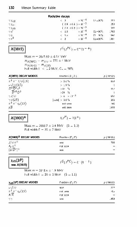
130130130130 Meson Summary TableRadiative de aysRadiative de aysRadiative de aysRadiative de aysγχ 2 < 9 × 10⁻⁴ CL=90% 211γχ 1 ( 2.9 ±0.6 )× 10−3 253γχ 0 ( 7.3 ±0.9 )× 10−3 341γ η′ < 1.8 × 10⁻⁴ CL=90% 1765γ η < 1.5 × 10⁻⁴ CL=90% 1847γπ0 < 2 × 10⁻⁴ CL=90% 1884X (3872)X (3872)X (3872)X (3872) IG (JPC ) = 0+(1 + +)Mass m = 3871.69 ± 0.17 MeVmX (3872) − mJ/ψ = 775 ± 4 MeVmX (3872) − mψ(2S)Full width < 1.2 MeV, CL = 90%X (3872) DECAY MODESX (3872) DECAY MODESX (3872) DECAY MODESX (3872) DECAY MODES Fra tion (i /) p (MeV/ )π+π− J/ψ(1S) > 2.6 % 650ωJ/ψ(1S) > 1.9 % †D0D0π0 >32 % 117D∗0D0 >24 % †γ J/ψ > 6 × 10⁻³ 697γψ(2S) [xxaa > 3.0 % 181π+π−η (1S) not seen 746pp not seen 1693X (3900)±X (3900)±X (3900)±X (3900)± I (JP ) = ?(1+)Mass m = 3888.7 ± 3.4 MeV (S = 1.3)Full width = 35 ± 7 MeVX (3900)± DECAY MODESX (3900)± DECAY MODESX (3900)± DECAY MODESX (3900)± DECAY MODES Fra tion (i /) p (MeV/ )J/ψπ± seen 700h π± not seen (DD∗)± seen χ 0(2P)χ 0(2P)χ 0(2P)χ 0(2P)was X (3915)was X (3915)was X (3915)was X (3915) IG (JPC ) = 0+(0 + +)Mass m = 3918.4 ± 1.9 MeVFull width = 20 ± 5 MeV (S = 1.1)
χ 0(2P) DECAY MODESχ 0(2P) DECAY MODESχ 0(2P) DECAY MODESχ 0(2P) DECAY MODES Fra tion (i /) p (MeV/ )ωJ/ψ seen 222π+π−η (1S) not seen 785K K not seen γ γ seen 1959
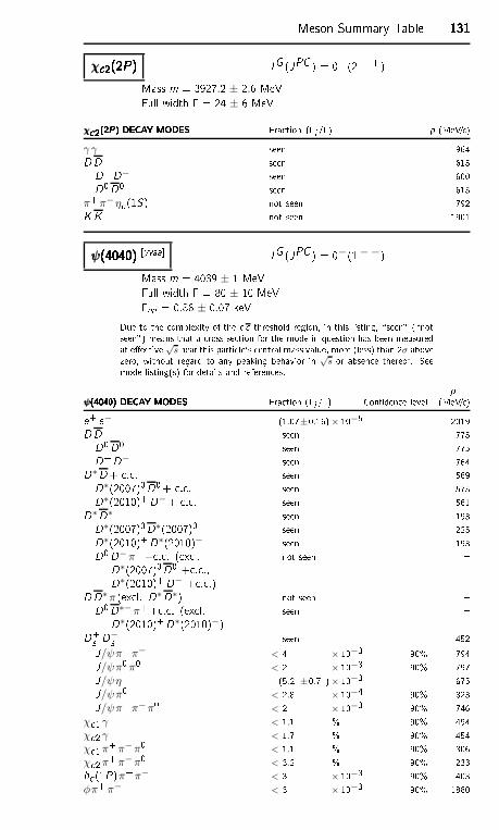
Meson Summary Table 131131131131χ 2(2P)χ 2(2P)χ 2(2P)χ 2(2P) IG (JPC ) = 0+(2 + +)Mass m = 3927.2 ± 2.6 MeVFull width = 24 ± 6 MeV
χ 2(2P) DECAY MODESχ 2(2P) DECAY MODESχ 2(2P) DECAY MODESχ 2(2P) DECAY MODES Fra tion (i /) p (MeV/ )γ γ seen 1964DD seen 615D+D− seen 600D0D0 seen 615π+π−η (1S) not seen 792K K not seen 1901ψ(4040)ψ(4040)ψ(4040)ψ(4040) [yyaa IG (JPC ) = 0−(1−−)Mass m = 4039 ± 1 MeVFull width = 80 ± 10 MeVee = 0.86 ± 0.07 keVDue to the omplexity of the threshold region, in this listing, \seen" (\notseen") means that a ross se tion for the mode in question has been measuredat ee tive √s near this parti le's entral mass value, more (less) than 2σ abovezero, without regard to any peaking behavior in √
s or absen e thereof. Seemode listing(s) for details and referen es. pψ(4040) DECAY MODESψ(4040) DECAY MODESψ(4040) DECAY MODESψ(4040) DECAY MODES Fra tion (i /) Conden e level (MeV/ )e+ e− (1.07±0.16)× 10−5 2019DD seen 775D0D0 seen 775D+D− seen 764D∗D+ . . seen 569D∗(2007)0D0+ . . seen 575D∗(2010)+D−+ . . seen 561D∗D∗ seen 193D∗(2007)0D∗(2007)0 seen 225D∗(2010)+D∗(2010)− seen 193D0D−π++ . . (ex l.D∗(2007)0D0 + . .,D∗(2010)+D− + . .) not seen DD∗π (ex l. D∗D∗) not seen D0D∗−π++ . . (ex l.D∗(2010)+D∗(2010)−) seen D+s D−s seen 452J/ψπ+π− < 4 × 10⁻³ 90% 794J/ψπ0π0 < 2 × 10⁻³ 90% 797J/ψη (5.2 ±0.7 )× 10−3 675J/ψπ0 < 2.8 × 10⁻⁴ 90% 823J/ψπ+π−π0 < 2 × 10⁻³ 90% 746χ 1 γ < 1.1 % 90% 494χ 2 γ < 1.7 % 90% 454χ 1π+π−π0 < 1.1 % 90% 306χ 2π+π−π0 < 3.2 % 90% 233h (1P)π+π− < 3 × 10⁻³ 90% 403φπ+π− < 3 × 10⁻³ 90% 1880
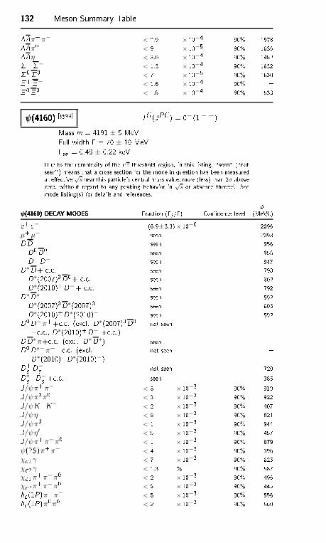
132132132132 Meson Summary Tableπ+π− < 2.9 × 10⁻⁴ 90% 1578π0 < 9 × 10⁻⁵ 90% 1636η < 3.0 × 10⁻⁴ 90% 1452+− < 1.3 × 10⁻⁴ 90% 163200 < 7 × 10⁻⁵ 90% 1630+− < 1.6 × 10⁻⁴ 90% 0 0 < 1.8 × 10⁻⁴ 90% 1533ψ(4160)ψ(4160)ψ(4160)ψ(4160) [yyaa IG (JPC ) = 0−(1−−)Mass m = 4191 ± 5 MeVFull width = 70 ± 10 MeVee = 0.48 ± 0.22 keVDue to the omplexity of the threshold region, in this listing, \seen" (\notseen") means that a ross se tion for the mode in question has been measuredat ee tive √s near this parti le's entral mass value, more (less) than 2σ abovezero, without regard to any peaking behavior in √
s or absen e thereof. Seemode listing(s) for details and referen es. pψ(4160) DECAY MODESψ(4160) DECAY MODESψ(4160) DECAY MODESψ(4160) DECAY MODES Fra tion (i /) Conden e level (MeV/ )e+ e− (6.9±3.3)× 10−6 2096µ+µ− seen 2093DD seen 956D0D0 seen 956D+D− seen 947D∗D+ . . seen 798D∗(2007)0D0+ . . seen 802D∗(2010)+D−+ . . seen 792D∗D∗ seen 592D∗(2007)0D∗(2007)0 seen 603D∗(2010)+D∗(2010)− seen 592D0D−π++ . . (ex l. D∗(2007)0D0+ . ., D∗(2010)+D− + . .) not seen DD∗π+ . . (ex l. D∗D∗) seen D0D∗−π++ . . (ex l.D∗(2010)+D∗(2010)−) not seen D+s D−s not seen 720D∗+s D−s + . . seen 385J/ψπ+π− < 3 × 10⁻³ 90% 919J/ψπ0π0 < 3 × 10⁻³ 90% 922J/ψK+K− < 2 × 10⁻³ 90% 407J/ψη < 8 × 10⁻³ 90% 821J/ψπ0 < 1 × 10⁻³ 90% 944J/ψη′ < 5 × 10⁻³ 90% 457J/ψπ+π−π0 < 1 × 10⁻³ 90% 879ψ(2S)π+π− < 4 × 10⁻³ 90% 396χ 1 γ < 7 × 10⁻³ 90% 625χ 2 γ < 1.3 % 90% 587χ 1π+π−π0 < 2 × 10⁻³ 90% 496χ 2π+π−π0 < 8 × 10⁻³ 90% 445h (1P)π+π− < 5 × 10⁻³ 90% 556h (1P)π0π0 < 2 × 10⁻³ 90% 560
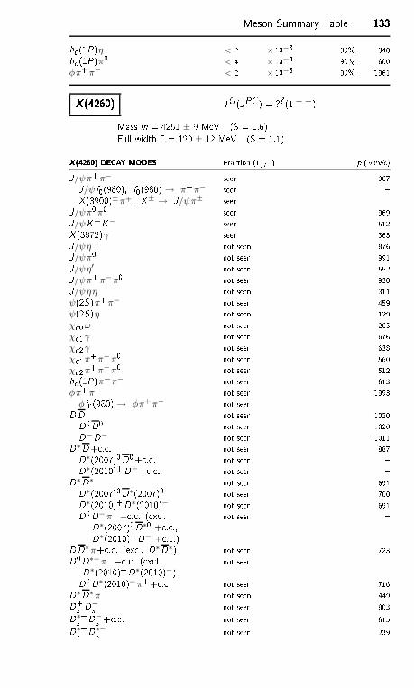
Meson Summary Table 133133133133h (1P)η < 2 × 10⁻³ 90% 348h (1P)π0 < 4 × 10⁻⁴ 90% 600φπ+π− < 2 × 10⁻³ 90% 1961X (4260)X (4260)X (4260)X (4260) IG (JPC ) = ??(1−−)Mass m = 4251 ± 9 MeV (S = 1.6)Full width = 120 ± 12 MeV (S = 1.1)X (4260) DECAY MODESX (4260) DECAY MODESX (4260) DECAY MODESX (4260) DECAY MODES Fra tion (i /) p (MeV/ )J/ψπ+π− seen 967J/ψ f0(980), f0(980) → π+π− seen X (3900)±π∓, X± → J/ψπ± seen J/ψπ0π0 seen 969J/ψK+K− seen 512X (3872)γ seen 363J/ψη not seen 876J/ψπ0 not seen 991J/ψη′ not seen 552J/ψπ+π−π0 not seen 930J/ψηη not seen 311ψ(2S)π+π− not seen 459ψ(2S)η not seen 129χ 0ω not seen 265χ 1 γ not seen 676χ 2 γ not seen 638χ 1π+π−π0 not seen 560χ 2π+π−π0 not seen 512h (1P)π+π− not seen 613φπ+π− not seen 1993
φ f0(980) → φπ+π− not seen DD not seen 1020D0D0 not seen 1020D+D− not seen 1011D∗D+ . . not seen 887D∗(2007)0D0+ . . not seen D∗(2010)+D−+ . . not seen D∗D∗ not seen 691D∗(2007)0D∗(2007)0 not seen 700D∗(2010)+D∗(2010)− not seen 691D0D−π++ . . (ex l.D∗(2007)0D∗0 + . .,D∗(2010)+D− + . .) not seen DD∗π+ . . (ex l. D∗D∗) not seen 723D0D∗−π++ . . (ex l.D∗(2010)+D∗(2010)−) not seen D0D∗(2010)−π++ . . not seen 716D∗D∗π not seen 449D+s D−s not seen 803D∗+s D−s + . . not seen 615D∗+s D∗−s not seen 239
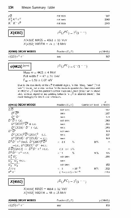
134134134134 Meson Summary Tablepp not seen 1907K0S K±π∓ not seen 2048K+K−π0 not seen 2049X (4360)X (4360)X (4360)X (4360) IG (JPC ) = ??(1−−)X (4360) MASS = 4361 ± 13 MeVX (4360) WIDTH = 74 ± 18 MeVX (4360) DECAY MODESX (4360) DECAY MODESX (4360) DECAY MODESX (4360) DECAY MODES Fra tion (i /) p (MeV/ )ψ(2S)π+π− seen 567ψ(4415)ψ(4415)ψ(4415)ψ(4415) [yyaa IG (JPC ) = 0−(1−−)Mass m = 4421 ± 4 MeVFull width = 62 ± 20 MeVee = 0.58 ± 0.07 keVDue to the omplexity of the threshold region, in this listing, \seen" (\notseen") means that a ross se tion for the mode in question has been measuredat ee tive √s near this parti le's entral mass value, more (less) than 2σ abovezero, without regard to any peaking behavior in √
s or absen e thereof. Seemode listing(s) for details and referen es. pψ(4415) DECAY MODESψ(4415) DECAY MODESψ(4415) DECAY MODESψ(4415) DECAY MODES Fra tion (i /) Conden e level (MeV/ )DD not seen 1187D0D0 seen 1187D+D− seen 1179D∗D+ . . not seen 1063D∗(2007)0D0+ . . seen 1066D∗(2010)+D−+ . . seen 1059D∗D∗ not seen 919D∗(2007)0D∗(2007)0+ . . seen 927D∗(2010)+D∗(2010)−+ . . seen 919D0D−π+ (ex l. D∗(2007)0D0+ . ., D∗(2010)+D− + . . < 2.3 % 90% DD∗2(2460) → D0D−π++ . . (10 ±4 ) % D0D∗−π++ . . < 11 % 90% 926D+s D−s not seen 1006D∗+s D−s + . . seen D∗+s D∗−s not seen 652J/ψη < 6 × 10⁻³ 90% 1022e+ e− ( 9.4±3.2)× 10−6 2210X (4660)X (4660)X (4660)X (4660) IG (JPC ) = ??(1−−)X (4660) MASS = 4664 ± 12 MeVX (4660) WIDTH = 48 ± 15 MeVX (4660) DECAY MODESX (4660) DECAY MODESX (4660) DECAY MODESX (4660) DECAY MODES Fra tion (i /) p (MeV/ )ψ(2S)π+π− seen 838
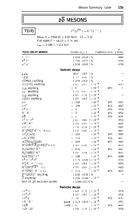
Meson Summary Table 135135135135bb MESONSbb MESONSbb MESONSbb MESONS(1S)(1S)(1S)(1S) IG (JPC ) = 0−(1−−)Mass m = 9460.30 ± 0.26 MeV (S = 3.3)Full width = 54.02 ± 1.25 keVee = 1.340 ± 0.018 keV p(1S) DECAY MODES(1S) DECAY MODES(1S) DECAY MODES(1S) DECAY MODES Fra tion (i /) Conden e level (MeV/ )τ+ τ− ( 2.60 ±0.10 ) % 4384e+ e− ( 2.38 ±0.11 ) % 4730µ+µ− ( 2.48 ±0.05 ) % 4729Hadroni de aysHadroni de aysHadroni de aysHadroni de aysg g g (81.7 ±0.7 ) % γ g g ( 2.2 ±0.6 ) % η′(958) anything ( 2.94 ±0.24 ) % J/ψ(1S) anything ( 6.5 ±0.7 )× 10−4 4223χ 0 anything < 5 × 10⁻³ 90% χ 1 anything ( 2.3 ±0.7 )× 10−4 χ 2 anything ( 3.4 ±1.0 )× 10−4 ψ(2S) anything ( 2.7 ±0.9 )× 10−4 ρπ < 3.68 × 10⁻⁶ 90% 4697ωπ0 < 3.90 × 10⁻⁶ 90% 4697π+π− < 5 × 10⁻⁴ 90% 4728K+K− < 5 × 10⁻⁴ 90% 4704pp < 5 × 10⁻⁴ 90% 4636π+π−π0 ( 2.1 ±0.8 )× 10−6 4725φK+K− ( 2.4 ±0.5 )× 10−6 4622ωπ+π− ( 4.5 ±1.0 )× 10−6 4694K∗(892)0K−π++ . . ( 4.4 ±0.8 )× 10−6 4667φ f ′2(1525) < 1.63 × 10⁻⁶ 90% 4549ω f2(1270) < 1.79 × 10⁻⁶ 90% 4611ρ(770)a2(1320) < 2.24 × 10⁻⁶ 90% 4605K∗(892)0K∗2(1430)0+ . . ( 3.0 ±0.8 )× 10−6 4579K1(1270)±K∓ < 2.41 × 10⁻⁶ 90% 4631K1(1400)±K∓ ( 1.0 ±0.4 )× 10−6 4613b1(1235)±π∓ < 1.25 × 10⁻⁶ 90% 4649π+π−π0π0 ( 1.28 ±0.30 )× 10−5 4720K0S K+π−+ . . ( 1.6 ±0.4 )× 10−6 4696K∗(892)0K0+ . . ( 2.9 ±0.9 )× 10−6 4675K∗(892)−K++ . . < 1.11 × 10⁻⁶ 90% 4675D∗(2010)± anything ( 2.52 ±0.20 ) % d anything ( 2.86 ±0.28 )× 10−5 Sum of 100 ex lusive modes ( 1.200±0.017) % Radiative de aysRadiative de aysRadiative de aysRadiative de aysγπ+π− ( 6.3 ±1.8 )× 10−5 4728γπ0π0 ( 1.7 ±0.7 )× 10−5 4728γπ0 η < 2.4 × 10⁻⁶ 90% 4713γK+K− [zzaa ( 1.14 ±0.13 )× 10−5 4704γ pp [aabb < 6 × 10⁻⁶ 90% 4636γ 2h+2h− ( 7.0 ±1.5 )× 10−4 4720
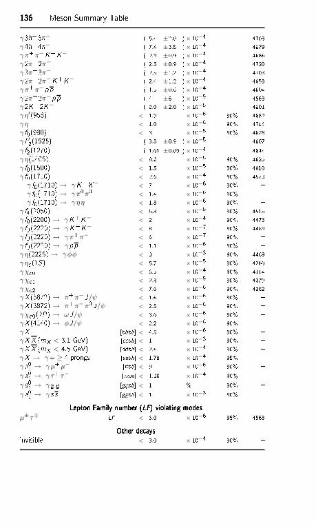
136136136136 Meson Summary Tableγ 3h+3h− ( 5.4 ±2.0 )× 10−4 4703γ 4h+4h− ( 7.4 ±3.5 )× 10−4 4679γπ+π−K+K− ( 2.9 ±0.9 )× 10−4 4686γ 2π+2π− ( 2.5 ±0.9 )× 10−4 4720γ 3π+3π− ( 2.5 ±1.2 )× 10−4 4703γ 2π+2π−K+K− ( 2.4 ±1.2 )× 10−4 4658γπ+π−pp ( 1.5 ±0.6 )× 10−4 4604γ 2π+2π−pp ( 4 ±6 )× 10−5 4563γ 2K+2K− ( 2.0 ±2.0 )× 10−5 4601γ η′(958) < 1.9 × 10⁻⁶ 90% 4682γ η < 1.0 × 10⁻⁶ 90% 4714γ f0(980) < 3 × 10⁻⁵ 90% 4678γ f ′2(1525) ( 3.8 ±0.9 )× 10−5 4607γ f2(1270) ( 1.01 ±0.09 )× 10−4 4644γ η(1405) < 8.2 × 10⁻⁵ 90% 4625γ f0(1500) < 1.5 × 10⁻⁵ 90% 4610γ f0(1710) < 2.6 × 10⁻⁴ 90% 4573
γ f0(1710) → γK+K− < 7 × 10⁻⁶ 90% γ f0(1710) → γπ0π0 < 1.4 × 10⁻⁶ 90% γ f0(1710) → γ ηη < 1.8 × 10⁻⁶ 90%
γ f4(2050) < 5.3 × 10⁻⁵ 90% 4515γ f0(2200) → γK+K− < 2 × 10⁻⁴ 90% 4475γ fJ (2220) → γK+K− < 8 × 10⁻⁷ 90% 4469γ fJ (2220) → γπ+π− < 6 × 10⁻⁷ 90% γ fJ (2220) → γ pp < 1.1 × 10⁻⁶ 90% γ η(2225) → γφφ < 3 × 10⁻³ 90% 4469γ η (1S) < 5.7 × 10⁻⁵ 90% 4260γχ 0 < 6.5 × 10⁻⁴ 90% 4114γχ 1 < 2.3 × 10⁻⁵ 90% 4079γχ 2 < 7.6 × 10⁻⁶ 90% 4062γX (3872) → π+π− J/ψ < 1.6 × 10⁻⁶ 90% γX (3872) → π+π−π0 J/ψ < 2.8 × 10⁻⁶ 90% γχ 0(2P) → ωJ/ψ < 3.0 × 10⁻⁶ 90% γX (4140) → φJ/ψ < 2.2 × 10⁻⁶ 90% γX [bbbb < 4.5 × 10⁻⁶ 90% γX X (mX < 3.1 GeV) [ bb < 1 × 10⁻³ 90% γX X (mX < 4.5 GeV) [ddbb < 2.4 × 10⁻⁴ 90% γX → γ+ ≥ 4 prongs [eebb < 1.78 × 10⁻⁴ 95% γ a01 → γµ+µ− [bb < 9 × 10⁻⁶ 90% γ a01 → γ τ+ τ− [zzaa < 1.30 × 10⁻⁴ 90% γ a01 → γ g g [ggbb < 1 % 90% γ a01 → γ s s [ggbb < 1 × 10⁻³ 90% Lepton Family number (LF) violating modesLepton Family number (LF) violating modesLepton Family number (LF) violating modesLepton Family number (LF) violating modesµ± τ∓ LF < 6.0 × 10⁻⁶ 95% 4563Other de aysOther de aysOther de aysOther de aysinvisible < 3.0 × 10⁻⁴ 90%
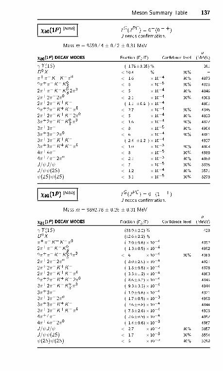
Meson Summary Table 137137137137χb0(1P)χb0(1P)χb0(1P)χb0(1P) [hhbb IG (JPC ) = 0+(0 + +)J needs onrmation.Mass m = 9859.44 ± 0.42 ± 0.31 MeV p
χb0(1P) DECAY MODESχb0(1P) DECAY MODESχb0(1P) DECAY MODESχb0(1P) DECAY MODES Fra tion (i /) Conden e level (MeV/ )γ(1S) ( 1.76±0.35) % 391D0X < 10.4 % 90% π+π−K+K−π0 < 1.6 × 10⁻⁴ 90% 48752π+π−K−K0S < 5 × 10⁻⁵ 90% 48752π+π−K−K0S 2π0 < 5 × 10⁻⁴ 90% 48462π+2π−2π0 < 2.1 × 10⁻⁴ 90% 49052π+2π−K+K− ( 1.1 ±0.6 )× 10−4 48612π+2π−K+K−π0 < 2.7 × 10⁻⁴ 90% 48462π+2π−K+K−2π0 < 5 × 10⁻⁴ 90% 48283π+2π−K−K0S π0 < 1.6 × 10⁻⁴ 90% 48273π+3π− < 8 × 10⁻⁵ 90% 49043π+3π−2π0 < 6 × 10⁻⁴ 90% 48813π+3π−K+K− ( 2.4 ±1.2 )× 10−4 48273π+3π−K+K−π0 < 1.0 × 10⁻³ 90% 48084π+4π− < 8 × 10⁻⁵ 90% 48804π+4π−2π0 < 2.1 × 10⁻³ 90% 4850J/ψJ/ψ < 7 × 10⁻⁵ 90% 3836J/ψψ(2S) < 1.2 × 10⁻⁴ 90% 3571ψ(2S)ψ(2S) < 3.1 × 10⁻⁵ 90% 3273χb1(1P)χb1(1P)χb1(1P)χb1(1P) [hhbb IG (JPC ) = 0+(1 + +)J needs onrmation.Mass m = 9892.78 ± 0.26 ± 0.31 MeV p
χb1(1P) DECAY MODESχb1(1P) DECAY MODESχb1(1P) DECAY MODESχb1(1P) DECAY MODES Fra tion (i /) Conden e level (MeV/ )γ(1S) (33.9±2.2) % 423D0X (12.6±2.2) % π+π−K+K−π0 ( 2.0±0.6)× 10−4 48922π+π−K−K0S ( 1.3±0.5)× 10−4 48922π+π−K−K0S 2π0 < 6 × 10⁻⁴ 90% 48632π+2π−2π0 ( 8.0±2.5)× 10−4 49212π+2π−K+K− ( 1.5±0.5)× 10−4 48782π+2π−K+K−π0 ( 3.5±1.2)× 10−4 48632π+2π−K+K−2π0 ( 8.6±3.2)× 10−4 48453π+2π−K−K0S π0 ( 9.3±3.3)× 10−4 48443π+3π− ( 1.9±0.6)× 10−4 49213π+3π−2π0 ( 1.7±0.5)× 10−3 48983π+3π−K+K− ( 2.6±0.8)× 10−4 48443π+3π−K+K−π0 ( 7.5±2.6)× 10−4 48254π+4π− ( 2.6±0.9)× 10−4 48974π+4π−2π0 ( 1.4±0.6)× 10−3 4867J/ψJ/ψ < 2.7 × 10⁻⁵ 90% 3857J/ψψ(2S) < 1.7 × 10⁻⁵ 90% 3594ψ(2S)ψ(2S) < 6 × 10⁻⁵ 90% 3298
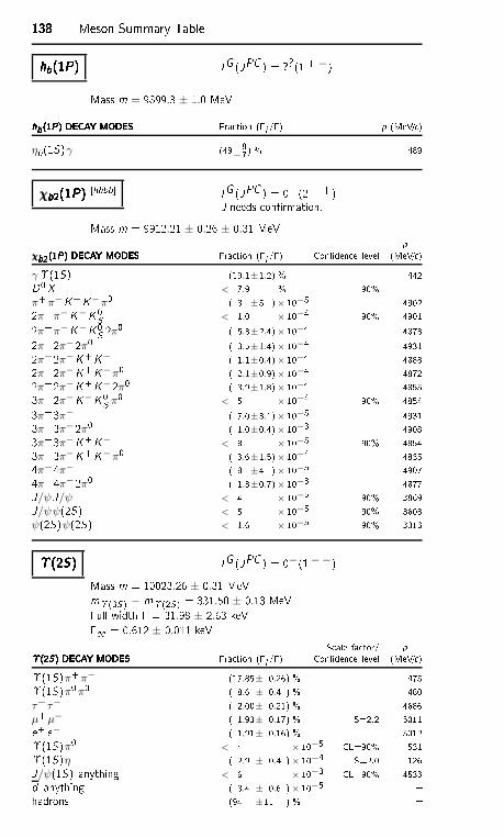
138138138138 Meson Summary Tablehb(1P)hb(1P)hb(1P)hb(1P) IG (JPC ) = ??(1 +−)Mass m = 9899.3 ± 1.0 MeVhb(1P) DECAY MODEShb(1P) DECAY MODEShb(1P) DECAY MODEShb(1P) DECAY MODES Fra tion (i /) p (MeV/ )ηb(1S)γ (49+8
−7) % 489χb2(1P)χb2(1P)χb2(1P)χb2(1P) [hhbb IG (JPC ) = 0+(2 + +)J needs onrmation.Mass m = 9912.21 ± 0.26 ± 0.31 MeV p
χb2(1P) DECAY MODESχb2(1P) DECAY MODESχb2(1P) DECAY MODESχb2(1P) DECAY MODES Fra tion (i /) Conden e level (MeV/ )γ(1S) (19.1±1.2) % 442D0X < 7.9 % 90% π+π−K+K−π0 ( 8 ±5 )× 10−5 49022π+π−K−K0S < 1.0 × 10⁻⁴ 90% 49012π+π−K−K0S 2π0 ( 5.3±2.4)× 10−4 48732π+2π−2π0 ( 3.5±1.4)× 10−4 49312π+2π−K+K− ( 1.1±0.4)× 10−4 48882π+2π−K+K−π0 ( 2.1±0.9)× 10−4 48722π+2π−K+K−2π0 ( 3.9±1.8)× 10−4 48553π+2π−K−K0S π0 < 5 × 10⁻⁴ 90% 48543π+3π− ( 7.0±3.1)× 10−5 49313π+3π−2π0 ( 1.0±0.4)× 10−3 49083π+3π−K+K− < 8 × 10⁻⁵ 90% 48543π+3π−K+K−π0 ( 3.6±1.5)× 10−4 48354π+4π− ( 8 ±4 )× 10−5 49074π+4π−2π0 ( 1.8±0.7)× 10−3 4877J/ψJ/ψ < 4 × 10⁻⁵ 90% 3869J/ψψ(2S) < 5 × 10⁻⁵ 90% 3608ψ(2S)ψ(2S) < 1.6 × 10⁻⁵ 90% 3313(2S)(2S)(2S)(2S) IG (JPC ) = 0−(1−−)Mass m = 10023.26 ± 0.31 MeVm(3S) − m(2S) = 331.50 ± 0.13 MeVFull width = 31.98 ± 2.63 keVee = 0.612 ± 0.011 keV S ale fa tor/ p(2S) DECAY MODES(2S) DECAY MODES(2S) DECAY MODES(2S) DECAY MODES Fra tion (i /) Conden e level (MeV/ )(1S)π+π− (17.85± 0.26) % 475(1S)π0π0 ( 8.6 ± 0.4 ) % 480τ+ τ− ( 2.00± 0.21) % 4686µ+µ− ( 1.93± 0.17) % S=2.2 5011e+ e− ( 1.91± 0.16) % 5012(1S)π0 < 4 × 10⁻⁵ CL=90% 531(1S)η ( 2.9 ± 0.4 )× 10−4 S=2.0 126J/ψ(1S) anything < 6 × 10⁻³ CL=90% 4533d anything ( 3.4 ± 0.6 )× 10−5 hadrons (94 ±11 ) %
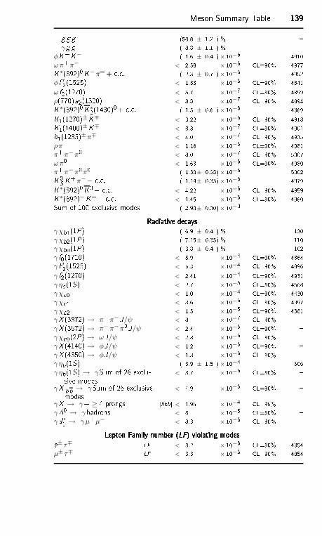
Meson Summary Table 139139139139g g g (58.8 ± 1.2 ) % γ g g ( 8.8 ± 1.1 ) %
φK+K− ( 1.6 ± 0.4 )× 10−6 4910ωπ+π− < 2.58 × 10⁻⁶ CL=90% 4977K∗(892)0K−π++ . . ( 2.3 ± 0.7 )× 10−6 4952φ f ′2(1525) < 1.33 × 10⁻⁶ CL=90% 4841ω f2(1270) < 5.7 × 10⁻⁷ CL=90% 4899ρ(770)a2(1320) < 8.8 × 10⁻⁷ CL=90% 4894K∗(892)0K∗2(1430)0+ . . ( 1.5 ± 0.6 )× 10−6 4869K1(1270)±K∓ < 3.22 × 10⁻⁶ CL=90% 4918K1(1400)±K∓ < 8.3 × 10⁻⁷ CL=90% 4901b1(1235)±π∓ < 4.0 × 10⁻⁷ CL=90% 4935ρπ < 1.16 × 10⁻⁶ CL=90% 4981π+π−π0 < 8.0 × 10⁻⁷ CL=90% 5007ωπ0 < 1.63 × 10⁻⁶ CL=90% 4980π+π−π0π0 ( 1.30± 0.28)× 10−5 5002K0S K+π−+ . . ( 1.14± 0.33)× 10−6 4979K∗(892)0K0+ . . < 4.22 × 10⁻⁶ CL=90% 4959K∗(892)−K++ . . < 1.45 × 10⁻⁶ CL=90% 4960Sum of 100 ex lusive modes ( 2.90± 0.30)× 10−3 Radiative de aysRadiative de aysRadiative de aysRadiative de aysγχb1(1P) ( 6.9 ± 0.4 ) % 130γχb2(1P) ( 7.15± 0.35) % 110γχb0(1P) ( 3.8 ± 0.4 ) % 162γ f0(1710) < 5.9 × 10⁻⁴ CL=90% 4864γ f ′2(1525) < 5.3 × 10⁻⁴ CL=90% 4896γ f2(1270) < 2.41 × 10⁻⁴ CL=90% 4931γ η (1S) < 2.7 × 10⁻⁵ CL=90% 4568γχ 0 < 1.0 × 10⁻⁴ CL=90% 4430γχ 1 < 3.6 × 10⁻⁶ CL=90% 4397γχ 2 < 1.5 × 10⁻⁵ CL=90% 4381γX (3872) → π+π− J/ψ < 8 × 10⁻⁷ CL=90% γX (3872) → π+π−π0 J/ψ < 2.4 × 10⁻⁶ CL=90% γχ 0(2P) → ωJ/ψ < 2.8 × 10⁻⁶ CL=90% γX (4140) → φJ/ψ < 1.2 × 10⁻⁶ CL=90% γX (4350) → φJ/ψ < 1.3 × 10⁻⁶ CL=90% γ ηb(1S) ( 3.9 ± 1.5 )× 10−4 606γ ηb(1S) → γSum of 26 ex lu-sive modes < 3.7 × 10⁻⁶ CL=90% γX b b → γSum of 26 ex lusivemodes < 4.9 × 10⁻⁶ CL=90% γX → γ+ ≥ 4 prongs [iibb < 1.95 × 10⁻⁴ CL=95% γA0 → γ hadrons < 8 × 10⁻⁵ CL=90% γ a01 → γµ+µ− < 8.3 × 10⁻⁶ CL=90% Lepton Family number (LF) violating modesLepton Family number (LF) violating modesLepton Family number (LF) violating modesLepton Family number (LF) violating modese± τ∓ LF < 3.2 × 10⁻⁶ CL=90% 4854µ± τ∓ LF < 3.3 × 10⁻⁶ CL=90% 4854
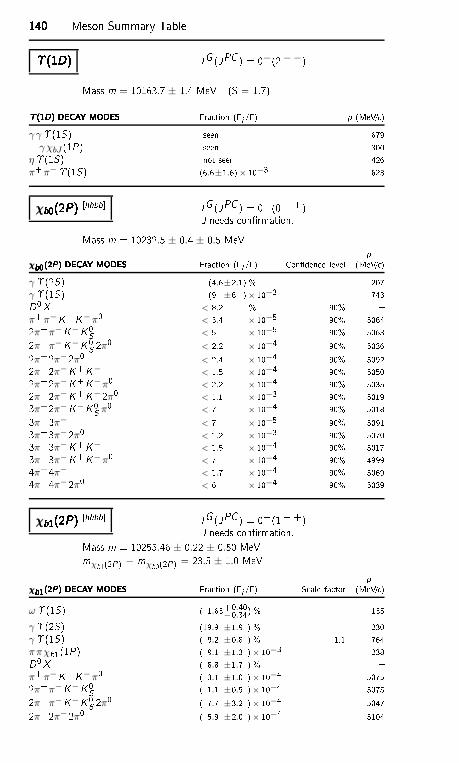
140140140140 Meson Summary Table(1D)(1D)(1D)(1D) IG (JPC ) = 0−(2−−)Mass m = 10163.7 ± 1.4 MeV (S = 1.7)(1D) DECAY MODES(1D) DECAY MODES(1D) DECAY MODES(1D) DECAY MODES Fra tion (i /) p (MeV/ )γ γ(1S) seen 679
γχbJ (1P) seen 300η(1S) not seen 426π+π−(1S) (6.6±1.6)× 10−3 623χb0(2P)χb0(2P)χb0(2P)χb0(2P) [hhbb IG (JPC ) = 0+(0 + +)J needs onrmation.Mass m = 10232.5 ± 0.4 ± 0.5 MeV p
χb0(2P) DECAY MODESχb0(2P) DECAY MODESχb0(2P) DECAY MODESχb0(2P) DECAY MODES Fra tion (i /) Conden e level (MeV/ )γ(2S) (4.6±2.1) % 207γ(1S) (9 ±6 )× 10−3 743D0X < 8.2 % 90% π+π−K+K−π0 < 3.4 × 10⁻⁵ 90% 50642π+π−K−K0S < 5 × 10⁻⁵ 90% 50632π+π−K−K0S 2π0 < 2.2 × 10⁻⁴ 90% 50362π+2π−2π0 < 2.4 × 10⁻⁴ 90% 50922π+2π−K+K− < 1.5 × 10⁻⁴ 90% 50502π+2π−K+K−π0 < 2.2 × 10⁻⁴ 90% 50352π+2π−K+K−2π0 < 1.1 × 10⁻³ 90% 50193π+2π−K−K0S π0 < 7 × 10⁻⁴ 90% 50183π+3π− < 7 × 10⁻⁵ 90% 50913π+3π−2π0 < 1.2 × 10⁻³ 90% 50703π+3π−K+K− < 1.5 × 10⁻⁴ 90% 50173π+3π−K+K−π0 < 7 × 10⁻⁴ 90% 49994π+4π− < 1.7 × 10⁻⁴ 90% 50694π+4π−2π0 < 6 × 10⁻⁴ 90% 5039χb1(2P)χb1(2P)χb1(2P)χb1(2P) [hhbb IG (JPC ) = 0+(1 + +)J needs onrmation.Mass m = 10255.46 ± 0.22 ± 0.50 MeVmχb1(2P) − mχb0(2P) = 23.5 ± 1.0 MeV p
χb1(2P) DECAY MODESχb1(2P) DECAY MODESχb1(2P) DECAY MODESχb1(2P) DECAY MODES Fra tion (i /) S ale fa tor (MeV/ )ω(1S) ( 1.63+0.40
−0.34) % 135γ(2S) (19.9 ±1.9 ) % 230γ(1S) ( 9.2 ±0.8 ) % 1.1 764ππχb1(1P) ( 9.1 ±1.3 )× 10−3 238D0X ( 8.8 ±1.7 ) % π+π−K+K−π0 ( 3.1 ±1.0 )× 10−4 50752π+π−K−K0S ( 1.1 ±0.5 )× 10−4 50752π+π−K−K0S 2π0 ( 7.7 ±3.2 )× 10−4 50472π+2π−2π0 ( 5.9 ±2.0 )× 10−4 5104
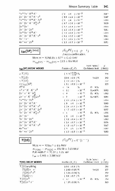
Meson Summary Table 1411411411412π+2π−K+K− (10 ±4 )× 10−5 50622π+2π−K+K−π0 ( 5.5 ±1.8 )× 10−4 50472π+2π−K+K−2π0 (10 ±4 )× 10−4 50303π+2π−K−K0S π0 ( 6.7 ±2.6 )× 10−4 50293π+3π− ( 1.2 ±0.4 )× 10−4 51033π+3π−2π0 ( 1.2 ±0.4 )× 10−3 50813π+3π−K+K− ( 2.0 ±0.8 )× 10−4 50293π+3π−K+K−π0 ( 6.1 ±2.2 )× 10−4 50114π+4π− ( 1.7 ±0.6 )× 10−4 50804π+4π−2π0 ( 1.9 ±0.7 )× 10−3 5051χb2(2P)χb2(2P)χb2(2P)χb2(2P) [hhbb IG (JPC ) = 0+(2 + +)J needs onrmation.Mass m = 10268.65 ± 0.22 ± 0.50 MeVmχb2(2P) − mχb1(2P) = 13.5 ± 0.6 MeV S ale fa tor/ p
χb2(2P) DECAY MODESχb2(2P) DECAY MODESχb2(2P) DECAY MODESχb2(2P) DECAY MODES Fra tion (i /) Conden e level (MeV/ )ω(1S) ( 1.10+0.34
−0.30) % 194γ(2S) (10.6 ±2.6 ) % S=2.0 242γ(1S) ( 7.0 ±0.7 ) % 777ππχb2(1P) ( 5.1 ±0.9 )× 10−3 229D0X < 2.4 % CL=90% π+π−K+K−π0 < 1.1 × 10⁻⁴ CL=90% 50822π+π−K−K0S < 9 × 10⁻⁵ CL=90% 50822π+π−K−K0S 2π0 < 7 × 10⁻⁴ CL=90% 50542π+2π−2π0 ( 3.9 ±1.6 )× 10−4 51102π+2π−K+K− ( 9 ±4 )× 10−5 50682π+2π−K+K−π0 ( 2.4 ±1.1 )× 10−4 50542π+2π−K+K−2π0 ( 4.7 ±2.3 )× 10−4 50373π+2π−K−K0S π0 < 4 × 10⁻⁴ CL=90% 50363π+3π− ( 9 ±4 )× 10−5 51103π+3π−2π0 ( 1.2 ±0.4 )× 10−3 50883π+3π−K+K− ( 1.4 ±0.7 )× 10−4 50363π+3π−K+K−π0 ( 4.2 ±1.7 )× 10−4 50174π+4π− ( 9 ±5 )× 10−5 50874π+4π−2π0 ( 1.3 ±0.5 )× 10−3 5058(3S)(3S)(3S)(3S) IG (JPC ) = 0−(1−−)Mass m = 10355.2 ± 0.5 MeVm(3S) − m(2S) = 331.50 ± 0.13 MeVFull width = 20.32 ± 1.85 keVee = 0.443 ± 0.008 keV S ale fa tor/ p(3S) DECAY MODES(3S) DECAY MODES(3S) DECAY MODES(3S) DECAY MODES Fra tion (i /) Conden e level (MeV/ )(2S)anything (10.6 ±0.8 ) % 296(2S)π+π− ( 2.82±0.18) % S=1.6 177(2S)π0π0 ( 1.85±0.14) % 190(2S)γ γ ( 5.0 ±0.7 ) % 327(2S)π0 < 5.1 × 10⁻⁴ CL=90% 298(1S)π+π− ( 4.37±0.08) % 813
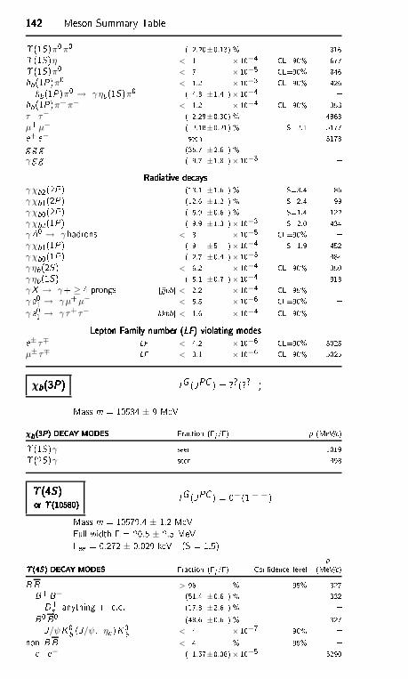
142142142142 Meson Summary Table(1S)π0π0 ( 2.20±0.13) % 816(1S)η < 1 × 10⁻⁴ CL=90% 677(1S)π0 < 7 × 10⁻⁵ CL=90% 846hb(1P)π0 < 1.2 × 10⁻³ CL=90% 426hb(1P)π0 → γ ηb(1S)π0 ( 4.3 ±1.4 )× 10−4 hb(1P)π+π− < 1.2 × 10⁻⁴ CL=90% 353τ+ τ− ( 2.29±0.30) % 4863µ+µ− ( 2.18±0.21) % S=2.1 5177e+ e− seen 5178g g g (35.7 ±2.6 ) % γ g g ( 9.7 ±1.8 )× 10−3 Radiative de aysRadiative de aysRadiative de aysRadiative de aysγχb2(2P) (13.1 ±1.6 ) % S=3.4 86γχb1(2P) (12.6 ±1.2 ) % S=2.4 99γχb0(2P) ( 5.9 ±0.6 ) % S=1.4 122γχb2(1P) ( 9.9 ±1.3 )× 10−3 S=2.0 434γA0 → γ hadrons < 8 × 10⁻⁵ CL=90% γχb1(1P) ( 9 ±5 )× 10−4 S=1.9 452γχb0(1P) ( 2.7 ±0.4 )× 10−3 484γ ηb(2S) < 6.2 × 10⁻⁴ CL=90% 350γ ηb(1S) ( 5.1 ±0.7 )× 10−4 913γX → γ+ ≥ 4 prongs [jjbb < 2.2 × 10⁻⁴ CL=95% γ a01 → γµ+µ− < 5.5 × 10⁻⁶ CL=90% γ a01 → γ τ+ τ− [kkbb < 1.6 × 10⁻⁴ CL=90% Lepton Family number (LF) violating modesLepton Family number (LF) violating modesLepton Family number (LF) violating modesLepton Family number (LF) violating modese± τ∓ LF < 4.2 × 10⁻⁶ CL=90% 5025µ± τ∓ LF < 3.1 × 10⁻⁶ CL=90% 5025χb(3P)χb(3P)χb(3P)χb(3P) IG (JPC ) = ??(??+)Mass m = 10534 ± 9 MeV
χb(3P) DECAY MODESχb(3P) DECAY MODESχb(3P) DECAY MODESχb(3P) DECAY MODES Fra tion (i /) p (MeV/ )(1S)γ seen 1019(2S)γ seen 498(4S)(4S)(4S)(4S)or (10580)or (10580)or (10580)or (10580) IG (JPC ) = 0−(1−−)Mass m = 10579.4 ± 1.2 MeVFull width = 20.5 ± 2.5 MeVee = 0.272 ± 0.029 keV (S = 1.5) p(4S) DECAY MODES(4S) DECAY MODES(4S) DECAY MODES(4S) DECAY MODES Fra tion (i /) Conden e level (MeV/ )BB > 96 % 95% 327B+B− (51.4 ±0.6 ) % 332D+s anything + . . (17.8 ±2.6 ) % B0B0 (48.6 ±0.6 ) % 327J/ψK0S (J/ψ, η )K0S < 4 × 10⁻⁷ 90% non-BB < 4 % 95% e+ e− ( 1.57±0.08)× 10−5 5290
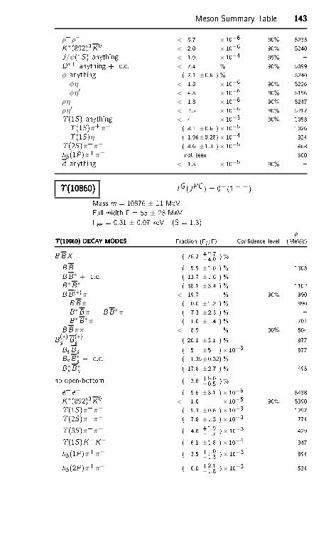
Meson Summary Table 143143143143ρ+ρ− < 5.7 × 10⁻⁶ 90% 5233K∗(892)0K0 < 2.0 × 10⁻⁶ 90% 5240J/ψ(1S) anything < 1.9 × 10⁻⁴ 95% D∗+ anything + . . < 7.4 % 90% 5099φ anything ( 7.1 ±0.6 ) % 5240
φη < 1.8 × 10⁻⁶ 90% 5226φη′ < 4.3 × 10⁻⁶ 90% 5196
ρη < 1.3 × 10⁻⁶ 90% 5247ρη′ < 2.5 × 10⁻⁶ 90% 5217(1S) anything < 4 × 10⁻³ 90% 1053(1S)π+π− ( 8.1 ±0.6 )× 10−5 1026(1S)η ( 1.96±0.28)× 10−4 924(2S)π+π− ( 8.6 ±1.3 )× 10−5 468hb(1P)π+π− not seen 600d anything < 1.3 × 10⁻⁵ 90% (10860)(10860)(10860)(10860) IG (JPC ) = 0−(1−−)Mass m = 10876 ± 11 MeVFull width = 55 ± 28 MeVee = 0.31 ± 0.07 keV (S = 1.3) p(10860) DECAY MODES(10860) DECAY MODES(10860) DECAY MODES(10860) DECAY MODES Fra tion (i /) Conden e level (MeV/ )BBX ( 76.2 +2.7
−4.0 ) % BB ( 5.5 ±1.0 ) % 1303BB∗ + . . ( 13.7 ±1.6 ) % B∗B∗ ( 38.1 ±3.4 ) % 1102BB(∗)π < 19.7 % 90% 990BB π ( 0.0 ±1.2 ) % 990B∗B π + BB∗π ( 7.3 ±2.3 ) % B∗B∗π ( 1.0 ±1.4 ) % 701BB ππ < 8.9 % 90% 504B(∗)s B(∗)s ( 20.1 ±3.1 ) % 877Bs Bs ( 5 ±5 )× 10−3 877Bs B∗s + . . ( 1.35±0.32) % B∗s B∗s ( 17.6 ±2.7 ) % 495no open-bottom ( 3.8 +5.0−0.5 ) % e+ e− ( 5.6 ±3.1 )× 10−6 5438K∗(892)0K0 < 1.0 × 10⁻⁵ 90% 5390(1S)π+π− ( 5.3 ±0.6 )× 10−3 1297(2S)π+π− ( 7.8 ±1.3 )× 10−3 774(3S)π+π− ( 4.8 +1.9−1.7 )× 10−3 429(1S)K+K− ( 6.1 ±1.8 )× 10−4 947hb(1P)π+π− ( 3.5 +1.0−1.3 )× 10−3 894hb(2P)π+π− ( 6.0 +2.1−1.8 )× 10−3 534
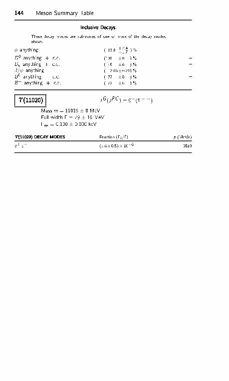
144144144144 Meson Summary TableIn lusive De ays.In lusive De ays.In lusive De ays.In lusive De ays.These de ay modes are submodes of one or more of the de ay modesabove.φ anything ( 13.8 +2.4
−1.7 ) % D0 anything + . . (108 ±8 ) % Ds anything + . . ( 46 ±6 ) % J/ψ anything ( 2.06±0.21) % B0 anything + . . ( 77 ±8 ) % B+ anything + . . ( 72 ±6 ) % (11020)(11020)(11020)(11020) IG (JPC ) = 0−(1−−)Mass m = 11019 ± 8 MeVFull width = 79 ± 16 MeVee = 0.130 ± 0.030 keV(11020) DECAY MODES(11020) DECAY MODES(11020) DECAY MODES(11020) DECAY MODES Fra tion (i /) p (MeV/ )e+ e− (1.6±0.5)× 10−6 5510
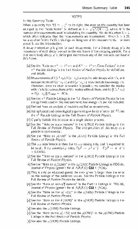
Meson Summary Table 145145145145NOTESIn this Summary Table:When a quantity has \(S = . . .)" to its right, the error on the quantity has beenenlarged by the \s ale fa tor" S, dened as S = √
χ2/(N − 1), where N is thenumber of measurements used in al ulating the quantity. We do this when S > 1,whi h often indi ates that the measurements are in onsistent. When S > 1.25,we also show in the Parti le Listings an ideogram of the measurements. For moreabout S, see the Introdu tion.A de ay momentum p is given for ea h de ay mode. For a 2-body de ay, p is themomentum of ea h de ay produ t in the rest frame of the de aying parti le. For a3-or-more-body de ay, p is the largest momentum any of the produ ts an have inthis frame.[a See the \Note on π± → ℓ±ν γ and K± → ℓ±ν γ Form Fa tors" in theπ± Parti le Listings in the Full Review of Parti le Physi s for denitionsand details.[b Measurements of (e+ νe)/(µ+ νµ) always in lude de ays with γ's, andmeasurements of (e+νe γ) and (µ+ νµ γ) never in lude low-energy γ's.Therefore, sin e no lean separation is possible, we onsider the modeswith γ's to be subrea tions of the modes without them, and let [(e+ νe )+ (µ+ νµ)/total = 100%.[ See the π± Parti le Listings in the Full Review of Parti le Physi s for theenergy limits used in this measurement; low-energy γ's are not in luded.[d Derived from an analysis of neutrino-os illation experiments.[e Astrophysi al and osmologi al arguments give limits of order 10−13; seethe π0 Parti le Listings in the Full Review of Parti le Physi s.[f C parity forbids this to o ur as a single-photon pro ess.[g See the \Note on s alar mesons" in the f0(500) Parti le Listings in theFull Review of Parti le Physi s. The interpretation of this entry as aparti le is ontroversial.[h See the \Note on ρ(770)" in the ρ(770) Parti le Listings in the FullReview of Parti le Physi s.[i The ωρ interferen e is then due to ωρ mixing only, and is expe ted tobe small. If eµ universality holds, (ρ0 → µ+µ−) = (ρ0 → e+ e−)× 0.99785.[j See the \Note on s alar mesons" in the f0(500) Parti le Listings in theFull Review of Parti le Physi s.[k See the \Note on a1(1260)" in the a1(1260) Parti le Listings in PDG 06,Journal of Physi s (generi for all A,B,E,G) G33G33G33G33 1 (2006).[l This is only an edu ated guess; the error given is larger than the erroron the average of the published values. See the Parti le Listings in theFull Review of Parti le Physi s for details.[n See the \Note on non-qq mesons" in the Parti le Listings in PDG 06,Journal of Physi s (generi for all A,B,E,G) G33G33G33G33 1 (2006).[o See the \Note on the η(1405)" in the η(1405) Parti le Listings in theFull Review of Parti le Physi s.[p See the \Note on the f1(1420)" in the η(1405) Parti le Listings in theFull Review of Parti le Physi s.[q See also the ω(1650) Parti le Listings.[r See the \Note on the ρ(1450) and the ρ(1700)" in the ρ(1700) Parti leListings in the Full Review of Parti le Physi s.[s See also the ω(1420) Parti le Listings.
146146146146 Meson Summary Table[t See the \Note on f0(1710)" in the f0(1710) Parti le Listings in 2004edition of Review of Parti le Physi s.[u See the note in the K± Parti le Listings in the Full Review of Parti lePhysi s.[v The denition of the slope parameter g of the K → 3π Dalitz plot is asfollows (see also \Note on Dalitz Plot Parameters for K → 3π De ays"in the K± Parti le Listings in the Full Review of Parti le Physi s):∣
∣M∣
∣
2 = 1 + g (s3 − s0)/m2π+ + · · · .[x For more details and denitions of parameters see Parti le Listings in theFull Review of Parti le Physi s.[y See the K± Parti le Listings in the Full Review of Parti le Physi s forthe energy limits used in this measurement.[z Most of this radiative mode, the low-momentum γ part, is also in ludedin the parent mode listed without γ's.[aa Stru ture-dependent part.[bb Dire t-emission bran hing fra tion.[ Violates angular-momentum onservation.[dd Derived from measured values of φ+−, φ00, ∣
∣η∣
∣, ∣
∣mK0L − mK0S ∣
∣, andτK0S , as des ribed in the introdu tion to \Tests of Conservation Laws."[ee The CP-violation parameters are dened as follows (see also \Note onCP Violation in KS → 3π" and \Note on CP Violation in K0L De ay"in the Parti le Listings in the Full Review of Parti le Physi s):
η+− = ∣
∣η+−∣
∣eiφ+− = A(K0L → π+π−)A(K0S → π+π−) = ǫ + ǫ′
η00 = ∣
∣η00∣∣eiφ00 = A(K0L → π0π0)A(K0S → π0π0) = ǫ − 2ǫ′δ = (K0L → π− ℓ+ν) − (K0L → π+ ℓ−ν)(K0L → π− ℓ+ν) + (K0L → π+ ℓ−ν) ,Im(η+−0)2 = (K0S → π+π−π0)CP viol.(K0L → π+π−π0) ,Im(η000)2 = (K0S → π0π0π0)(K0L → π0π0π0) .where for the last two relations CPT is assumed valid, i.e., Re(η+−0) ≃0 and Re(η000) ≃ 0.[ See the K0S Parti le Listings in the Full Review of Parti le Physi s forthe energy limits used in this measurement.[gg The value is for the sum of the harge states or parti le/antiparti lestates indi ated.[hh Re(ǫ′/ǫ) = ǫ′/ǫ to a very good approximation provided the phases satisfyCPT invarian e.[ii This mode in ludes gammas from inner bremsstrahlung but not the dire temission mode K0L → π+π− γ(DE).[jj See the K0L Parti le Listings in the Full Review of Parti le Physi s forthe energy limits used in this measurement.[kk Allowed by higher-order ele troweak intera tions.
Meson Summary Table 147147147147[ll Violates CP in leading order. Test of dire t CP violation sin e the in-dire t CP-violating and CP- onserving ontributions are expe ted to besuppressed.[nn See the \Note on f0(1370)" in the f0(1370) Parti le Listings in the FullReview of Parti le Physi s and in the 1994 edition.[oo See the note in the L(1770) Parti le Listings in Reviews of ModernPhysi s 56565656 S1 (1984), p. S200. See also the \Note on K2(1770) andthe K2(1820)" in the K2(1770) Parti le Listings in the Full Review ofParti le Physi s.[pp See the \Note on K2(1770) and the K2(1820)" in the K2(1770) Parti leListings in the Full Review of Parti le Physi s.[qq This result applies to Z0 → de ays only. Here ℓ+ is an average (nota sum) of e+ and µ+ de ays.[rr See the Parti le Listings for the ( ompli ated) denition of this quantity.[ss The bran hing fra tion for this mode may dier from the sum of thesubmodes that ontribute to it, due to interferen e ee ts. See therelevant papers in the Parti le Listings in the Full Review of Parti lePhysi s.[tt These subfra tions of the K−2π+ mode are un ertain: see the Parti leListings.[uu Submodes of the D+ → K−2π+π0 and K0S 2π+π− modes were studiedby ANJOS 92C and COFFMAN 92B, but with at most 142 events for therst mode and 229 for the se ond not enough for pre ise results. Withnothing new for 18 years, we refer to our 2008 edition, Physi s LettersB667B667B667B667 1 (2008), for those results.[vv The unseen de ay modes of the resonan es are in luded.[xx This is not a test for the C=1 weak neutral urrent, but leads to theπ+ ℓ+ ℓ− nal state.[yy This mode is not a useful test for a C=1 weak neutral urrent be auseboth quarks must hange avor in this de ay.[zz In the 2010 Review, the values for these quantities were given using ameasure of the asymmetry that was in onsistent with the usual denition.[aaa This value is obtained by subtra ting the bran hing fra tions for 2-, 4-and 6-prongs from unity.[bbb This is the sum of our K−2π+π−, K−2π+π−π0,K0 2π+2π−, K+2K−π+, 2π+2π−, 2π+2π−π0, K+K−π+π−, andK+K−π+π−π0, bran hing fra tions.[ This is the sum of our K−3π+2π− and 3π+3π− bran hing fra tions.[ddd The bran hing fra tions for the K− e+ νe , K∗(892)− e+νe , π− e+νe ,and ρ− e+ νe modes add up to 6.19 ± 0.17 %.[eee This is a doubly Cabibbo-suppressed mode.[f The two experiments measuring this fra tion are in serious disagreement.See the Parti le Listings in the Full Review of Parti le Physi s.[ggg Submodes of the D0 → K0S π+π−π0 mode with a K∗ and/or ρ werestudied by COFFMAN 92B, but with only 140 events. With nothing newfor 18 years, we refer to our 2008 edition, Physi s Letters B667B667B667B667 1 (2008),for those results.[hhh This bran hing fra tion in ludes all the de ay modes of the resonan e inthe nal state.[iii This limit is for either D0 or D0 to p e−.[jjj This limit is for either D0 or D0 to p e+.
148148148148 Meson Summary Table[kkk This is the purely e+ semileptoni bran hing fra tion: the e+ fra tionfrom τ+ de ays has been subtra ted o. The sum of our (non-τ) e+ex lusive fra tions | an e+νe with an η, η′, φ, K0, K∗0, or f0(980) |is 7.0 ± 0.4 %[lll This fra tion in ludes η from η′ de ays.[nnn Two times (to in lude µ de ays) the η′ e+ νe bran hing fra tion, plus theη′π+, η′ρ+, and η′K+ fra tions, is (18.6 ± 2.3)%, whi h onsiderablyex eeds the in lusive η′ fra tion of (11.7± 1.8)%. Our best guess is thatthe η′ρ+ fra tion, (12.5 ± 2.2)%, is too large.[ooo This bran hing fra tion in ludes all the de ay modes of the nal-stateresonan e.[ppp A test for uu or dd ontent in the D+s . Neither Cabibbo-favored norCabibbo-suppressed de ays an ontribute, and ω−φ mixing is an unlikelyexplanation for any fra tion above about 2× 10⁻⁴.[qqq We de ouple the D+s → φπ+ bran hing fra tion obtained from massproje tions (and used to get some of the other bran hing fra tions) fromthe D+s → φπ+, φ → K+K− bran hing fra tion obtained from theDalitz-plot analysis of D+s → K+K−π+. That is, the ratio of these twobran hing fra tions is not exa tly the φ → K+K− bran hing fra tion0.491.[rrr This is the average of a model-independent and a K-matrix parametriza-tion of the π+π− S-wave and is a sum over several f0 mesons.[sss An ℓ indi ates an e or a µ mode, not a sum over these modes.[ttt An CP(±1) indi ates the CP=+1 and CP=−1 eigenstates of the D0-D0system.[uuu D denotes D0 or D0.[vvv D∗0
CP+ de ays into D0π0 with the D0 re onstru ted in CP-even eigen-states K+K− and π+π−.[xxx D∗∗ represents an ex ited state with mass 2.2 < M < 2.8 GeV/ 2.[yyy X (3872)+ is a hypotheti al harged partner of the X (3872).[zzz (1710)++ is a possible narrow pentaquark state and G (2220) is apossible glueball resonan e.[aaaa (− p)s denotes a low-mass enhan ement near 3.35 GeV/ 2.[bbaa Stands for the possible andidates of K∗(1410), K∗0(1430) andK∗2(1430).[ aa B0 and B0s ontributions not separated. Limit is on weighted averageof the two de ay rates.[ddaa This de ay refers to the oherent sum of resonant and nonresonant JP= 0+ K π omponents with 1.60 < mK π < 2.15 GeV/ 2.[eeaa X (214) is a hypotheti al parti le of mass 214 MeV/ 2 reported by theHyperCP experiment, Physi al Review Letters 94949494 021801 (2005)[aa (1540)+ denotes a possible narrow pentaquark state.[ggaa Here S and P are the hypotheti al s alar and pseudos alar parti les withmasses of 2.5 GeV/ 2 and 214.3 MeV/ 2, respe tively.[hhaa These values are model dependent.[iiaa Here \anything" means at least one parti le observed.[jjaa This is a B(B0 → D∗− ℓ+νℓ) value.
Meson Summary Table 149149149149[kkaa D∗∗ stands for the sum of the D(1 1P1), D(1 3P0), D(1 3P1), D(1 3P2),D(2 1S0), and D(2 1S1) resonan es.[llaa D(∗)D(∗) stands for the sum of D∗D∗, D∗D, DD∗, and DD .[nnaa X (3915) denotes a near-threshold enhan ement in the ωJ/ψ mass spe -trum.[ooaa In lusive bran hing fra tions have a multipli ity denition and an begreater than 100%.[ppaa Dj represents an unresolved mixture of pseudos alar and tensor D∗∗(P-wave) states.[qqaa Not a pure measurement. See note at head of B0s De ay Modes.[rraa For Eγ > 100 MeV.[ssaa In ludes ppπ+π−γ and ex ludes ppη, ppω, ppη′.[ttaa For a narrow state A with mass less than 960 MeV.[uuaa For a narrow s alar or pseudos alar A0 with mass 0.213.0 GeV.[vvaa For a narrow resonan e in the range 2.2 < M(X ) < 2.8 GeV.[xxaa BHARDWAJ 11 does not observe this de ay and presents a stronger90% CL limit than this value. See measurements listings for details.[yyaa JPC known by produ tion in e+ e− via single photon annihilation. IGis not known; interpretation of this state as a single resonan e is un learbe ause of the expe tation of substantial threshold ee ts in this energyregion.[zzaa 2mτ < M(τ+ τ−) < 9.2 GeV[aabb 2 GeV < mK+K− < 3 GeV[bbbb X = s alar with m < 8.0 GeV[ bb X X = ve tors with m < 3.1 GeV[ddbb X and X = zero spin with m < 4.5 GeV[eebb 1.5 GeV < mX < 5.0 GeV[bb 201 MeV < M(µ+µ−) < 3565 MeV[ggbb 0.5 GeV < mX < 9.0 GeV, where mX is the invariant mass of thehadroni nal state.[hhbb Spe tros opi labeling for these states is theoreti al, pending experi-mental information.[iibb 1.5 GeV < mX < 5.0 GeV[jjbb 1.5 GeV < mX < 5.0 GeV[kkbb For mτ+ τ− in the ranges 4.039.52 and 9.6110.10 GeV.
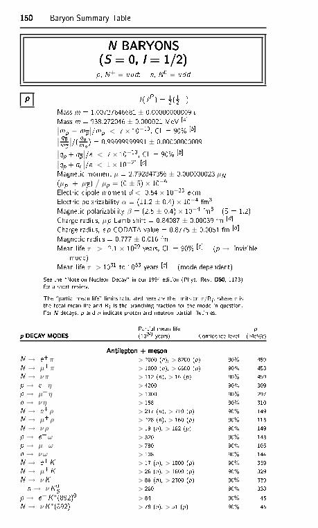
150150150150 Baryon Summary TableN BARYONSN BARYONSN BARYONSN BARYONS(S = 0, I = 1/2)(S = 0, I = 1/2)(S = 0, I = 1/2)(S = 0, I = 1/2)p, N+ = uud; n, N0 = uddpppp I (JP ) = 12 (12+)Mass m = 1.00727646681 ± 0.00000000009 uMass m = 938.272046 ± 0.000021 MeV [a∣
∣mp − mp∣∣/mp < 7× 10⁻¹⁰, CL = 90% [b∣
∣
qpmp ∣
∣/( qpmp ) = 0.99999999991 ± 0.00000000009∣
∣qp + qp∣
∣/e < 7× 10⁻¹⁰, CL = 90% [b∣
∣qp + qe ∣∣/e < 1× 10⁻²¹ [ Magneti moment µ = 2.792847356 ± 0.000000023 µN(µp + µp) /
µp = (0 ± 5)× 10−6Ele tri dipole moment d < 0.54× 10⁻²³ e mEle tri polarizability α = (11.2 ± 0.4)× 10−4 fm3Magneti polarizability β = (2.5 ± 0.4)× 10−4 fm3 (S = 1.2)Charge radius, µp Lamb shift = 0.84087 ± 0.00039 fm [dCharge radius, e p CODATA value = 0.8775 ± 0.0051 fm [dMagneti radius = 0.777 ± 0.016 fmMean life τ > 2.1 × 1029 years, CL = 90% [e (p → invisiblemode)Mean life τ > 1031 to 1033 years [e (mode dependent)See the \Note on Nu leon De ay" in our 1994 edition (Phys. Rev. D50D50D50D50, 1173)for a short review.The \partial mean life" limits tabulated here are the limits on τ/Bi , where τ isthe total mean life and Bi is the bran hing fra tion for the mode in question.For N de ays, p and n indi ate proton and neutron partial lifetimes.Partial mean life pp DECAY MODESp DECAY MODESp DECAY MODESp DECAY MODES (1030 years) Conden e level (MeV/ )Antilepton + mesonAntilepton + mesonAntilepton + mesonAntilepton + mesonN → e+π > 2000 (n), > 8200 (p) 90% 459N → µ+π > 1000 (n), > 6600 (p) 90% 453N → ν π > 112 (n), > 16 (p) 90% 459p → e+η > 4200 90% 309p → µ+η > 1300 90% 297n → ν η > 158 90% 310N → e+ρ > 217 (n), > 710 (p) 90% 149N → µ+ρ > 228 (n), > 160 (p) 90% 113N → ν ρ > 19 (n), > 162 (p) 90% 149p → e+ω > 320 90% 143p → µ+ω > 780 90% 105n → ν ω > 108 90% 144N → e+K > 17 (n), > 1000 (p) 90% 339N → µ+K > 26 (n), > 1600 (p) 90% 329N → νK > 86 (n), > 2300 (p) 90% 339n → νK0S > 260 90% 338p → e+K∗(892)0 > 84 90% 45N → νK∗(892) > 78 (n), > 51 (p) 90% 45
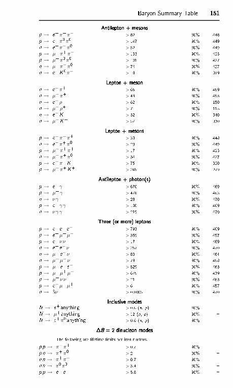
Baryon Summary Table 151151151151Antilepton + mesonsAntilepton + mesonsAntilepton + mesonsAntilepton + mesonsp → e+π+π− > 82 90% 448p → e+π0π0 > 147 90% 449n → e+π−π0> 52 90% 449p → µ+π+π− > 133 90% 425p → µ+π0π0 > 101 90% 427n → µ+π−π0 > 74 90% 427n → e+K0π− > 18 90% 319Lepton + mesonLepton + mesonLepton + mesonLepton + mesonn → e−π+ > 65 90% 459n → µ−π+ > 49 90% 453n → e− ρ+ > 62 90% 150n → µ− ρ+ > 7 90% 115n → e−K+ > 32 90% 340n → µ−K+ > 57 90% 330Lepton + mesonsLepton + mesonsLepton + mesonsLepton + mesonsp → e−π+π+ > 30 90% 448n → e−π+π0 > 29 90% 449p → µ−π+π+ > 17 90% 425n → µ−π+π0> 34 90% 427p → e−π+K+ > 75 90% 320p → µ−π+K+ > 245 90% 279Antilepton + photon(s)Antilepton + photon(s)Antilepton + photon(s)Antilepton + photon(s)p → e+γ > 670 90% 469p → µ+γ > 478 90% 463n → ν γ > 28 90% 470p → e+γ γ > 100 90% 469n → ν γ γ > 219 90% 470Three (or more) leptonsThree (or more) leptonsThree (or more) leptonsThree (or more) leptonsp → e+ e+ e− > 793 90% 469p → e+µ+µ− > 359 90% 457p → e+ν ν > 17 90% 469n → e+ e−ν > 257 90% 470n → µ+ e−ν > 83 90% 464n → µ+µ−ν > 79 90% 458p → µ+ e+ e− > 529 90% 463p → µ+µ+µ−> 675 90% 439p → µ+ν ν > 21 90% 463p → e−µ+µ+ > 6 90% 457n → 3ν > 0.0005 90% 470In lusive modesIn lusive modesIn lusive modesIn lusive modesN → e+ anything > 0.6 (n, p) 90% N → µ+anything > 12 (n, p) 90% N → e+π0 anything > 0.6 (n, p) 90% B = 2 dinu leon modesB = 2 dinu leon modesB = 2 dinu leon modesB = 2 dinu leon modesThe following are lifetime limits per iron nu leus.pp → π+π+ > 0.7 90% pn → π+π0> 2 90% nn → π+π− > 0.7 90% nn → π0π0 > 3.4 90% pp → e+ e+ > 5.8 90%
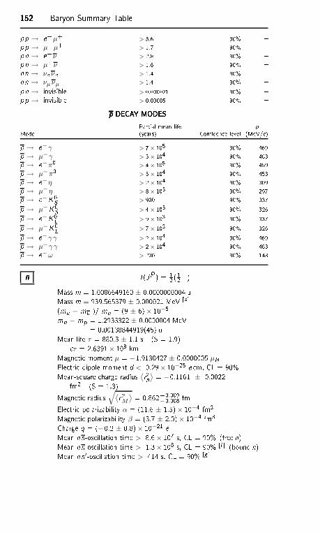
152152152152 Baryon Summary Tablepp → e+µ+ > 3.6 90% pp → µ+µ+ > 1.7 90% pn → e+ν > 2.8 90% pn → µ+ν > 1.6 90% nn → νe νe > 1.4 90% nn → νµ νµ > 1.4 90% pn → invisible > 0.000021 90% pp → invisible > 0.00005 90% p DECAY MODESp DECAY MODESp DECAY MODESp DECAY MODESPartial mean life pMode (years) Conden e level (MeV/ )p → e−γ > 7× 10⁵ 90% 469p → µ−γ > 5× 10⁴ 90% 463p → e−π0 > 4× 10⁵ 90% 459p → µ−π0 > 5× 10⁴ 90% 453p → e−η > 2× 10⁴ 90% 309p → µ−η > 8× 10³ 90% 297p → e−K0S > 900 90% 337p → µ−K0S > 4× 10³ 90% 326p → e−K0L > 9× 10³ 90% 337p → µ−K0L > 7× 10³ 90% 326p → e−γ γ > 2× 10⁴ 90% 469p → µ−γ γ > 2× 10⁴ 90% 463p → e−ω > 200 90% 143nnnn I (JP ) = 12 (12+)Mass m = 1.0086649160 ± 0.0000000004 uMass m = 939.565379 ± 0.000021 MeV [a(mn − mn )/ mn = (9 ± 6)× 10−5mn − mp = 1.2933322 ± 0.0000004 MeV= 0.00138844919(45) uMean life τ = 880.3 ± 1.1 s (S = 1.9) τ = 2.6391× 10⁸ kmMagneti moment µ = −1.9130427 ± 0.0000005 µNEle tri dipole moment d < 0.29× 10⁻²⁵ e m, CL = 90%Mean-square harge radius ⟨r2n⟩ = −0.1161 ± 0.0022fm2 (S = 1.3)Magneti radius √
⟨r2M ⟩ = 0.862+0.009−0.008 fmEle tri polarizability α = (11.6 ± 1.5)× 10−4 fm3Magneti polarizability β = (3.7 ± 2.0)× 10−4 fm3Charge q = (−0.2 ± 0.8)× 10−21 eMean nn-os illation time > 8.6× 10⁷ s, CL = 90% (free n)Mean nn-os illation time > 1.3× 10⁸ s, CL = 90% [f (bound n)Mean nn′-os illation time > 414 s, CL = 90% [g
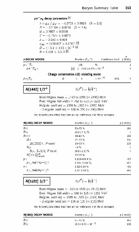
Baryon Summary Table 153153153153p e−νe de ay parametersp e−νe de ay parametersp e−νe de ay parametersp e−νe de ay parameters [hλ ≡ gA / gV = −1.2723 ± 0.0023 (S = 2.2)A = −0.1184 ± 0.0010 (S = 2.4)B = 0.9807 ± 0.0030C = −0.2377 ± 0.0026a = −0.103 ± 0.004φAV = (180.017 ± 0.026) [i D = (−1.2 ± 2.0)× 10−4 [jR = 0.004 ± 0.013 [j pn DECAY MODESn DECAY MODESn DECAY MODESn DECAY MODES Fra tion (i /) Conden e level (MeV/ )p e−νe 100 % 1p e−νe γ [k ( 3.09±0.32)× 10−3 1Charge onservation (Q) violating modeCharge onservation (Q) violating modeCharge onservation (Q) violating modeCharge onservation (Q) violating modepνe νe Q < 8 × 10⁻²⁷ 68% 1N(1440) 1/2+N(1440) 1/2+N(1440) 1/2+N(1440) 1/2+ I (JP ) = 12 (12+)Breit-Wigner mass = 1410 to 1450 (≈ 1430) MeVBreit-Wigner full width = 250 to 450 (≈ 350) MeVRe(pole position) = 1350 to 1380 (≈ 1365) MeV−2Im(pole position) = 160 to 220 (≈ 190) MeVThe following bran hing fra tions are our estimates, not ts or averages.N(1440) DECAY MODESN(1440) DECAY MODESN(1440) DECAY MODESN(1440) DECAY MODES Fra tion (i /) p (MeV/ )N π 5575 % 391N η (0.0±1.0) % †N ππ 3040 % 338π 2030 % 135(1232)π , P-wave 1530 % 135N ρ <8 % †N ρ , S=1/2, P-wave (0.0±1.0) % †N (ππ )I=0S-wave 1020 % pγ 0.0350.048 % 407pγ , heli ity=1/2 0.0350.048 % 407nγ 0.020.04 % 406nγ , heli ity=1/2 0.020.04 % 406N(1520) 3/2−N(1520) 3/2−N(1520) 3/2−N(1520) 3/2− I (JP ) = 12 (32−)Breit-Wigner mass = 1510 to 1520 (≈ 1515) MeVBreit-Wigner full width = 100 to 125 (≈ 115) MeVRe(pole position) = 1505 to 1515 (≈ 1510) MeV−2Im(pole position) = 105 to 120 (≈ 110) MeVThe following bran hing fra tions are our estimates, not ts or averages.N(1520) DECAY MODESN(1520) DECAY MODESN(1520) DECAY MODESN(1520) DECAY MODES Fra tion (i /) p (MeV/ )N π 5565 % 453N η (2.3±0.4)× 10−3 142
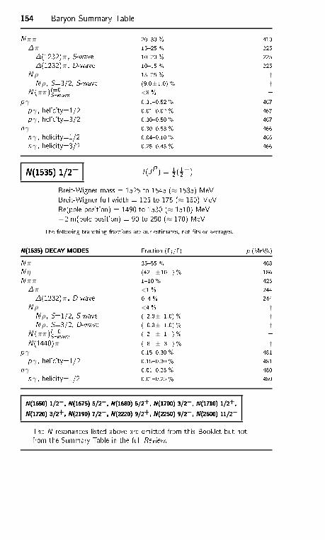
154154154154 Baryon Summary TableN ππ 2030 % 410π 1525 % 225(1232)π , S-wave 1020 % 225(1232)π , D-wave 1015 % 225N ρ 1525 % †N ρ , S=3/2, S-wave (9.0±1.0) % †N (ππ )I=0S-wave <8 % pγ 0.310.52 % 467pγ , heli ity=1/2 0.010.02 % 467pγ , heli ity=3/2 0.300.50 % 467nγ 0.300.53 % 466nγ , heli ity=1/2 0.040.10 % 466nγ , heli ity=3/2 0.250.45 % 466N(1535) 1/2−N(1535) 1/2−N(1535) 1/2−N(1535) 1/2− I (JP ) = 12 (12−)Breit-Wigner mass = 1525 to 1545 (≈ 1535) MeVBreit-Wigner full width = 125 to 175 (≈ 150) MeVRe(pole position) = 1490 to 1530 (≈ 1510) MeV−2Im(pole position) = 90 to 250 (≈ 170) MeVThe following bran hing fra tions are our estimates, not ts or averages.N(1535) DECAY MODESN(1535) DECAY MODESN(1535) DECAY MODESN(1535) DECAY MODES Fra tion (i /) p (MeV/ )N π 3555 % 468N η (42 ±10 ) % 186N ππ 110 % 426π <1 % 244(1232)π , D-wave 04 % 244N ρ <4 % †N ρ , S=1/2, S-wave ( 2.0± 1.0) % †N ρ , S=3/2, D-wave ( 0.0± 1.0) % †N (ππ )I=0S-wave ( 2 ± 1 ) % N(1440)π ( 8 ± 3 ) % †pγ 0.150.30 % 481pγ , heli ity=1/2 0.150.30 % 481nγ 0.010.25 % 480nγ , heli ity=1/2 0.010.25 % 480N(1650) 1/2−, N(1675) 5/2−, N(1680) 5/2+, N(1700) 3/2−, N(1710) 1/2+,N(1650) 1/2−, N(1675) 5/2−, N(1680) 5/2+, N(1700) 3/2−, N(1710) 1/2+,N(1650) 1/2−, N(1675) 5/2−, N(1680) 5/2+, N(1700) 3/2−, N(1710) 1/2+,N(1650) 1/2−, N(1675) 5/2−, N(1680) 5/2+, N(1700) 3/2−, N(1710) 1/2+,N(1720) 3/2+, N(2190) 7/2−, N(2220) 9/2+, N(2250) 9/2−, N(2600) 11/2−N(1720) 3/2+, N(2190) 7/2−, N(2220) 9/2+, N(2250) 9/2−, N(2600) 11/2−N(1720) 3/2+, N(2190) 7/2−, N(2220) 9/2+, N(2250) 9/2−, N(2600) 11/2−N(1720) 3/2+, N(2190) 7/2−, N(2220) 9/2+, N(2250) 9/2−, N(2600) 11/2−The N resonan es listed above are omitted from this Booklet but notfrom the Summary Table in the full Review.
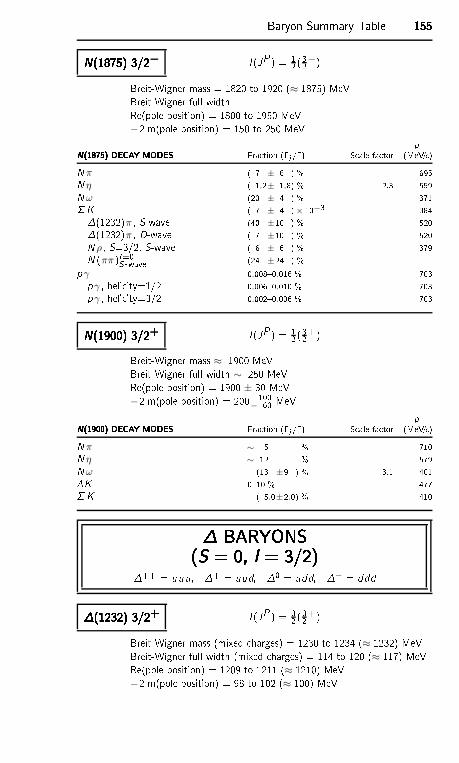
Baryon Summary Table 155155155155N(1875) 3/2−N(1875) 3/2−N(1875) 3/2−N(1875) 3/2− I (JP ) = 12 (32−)Breit-Wigner mass = 1820 to 1920 (≈ 1875) MeVBreit-Wigner full widthRe(pole position) = 1800 to 1950 MeV−2Im(pole position) = 150 to 250 MeV pN(1875) DECAY MODESN(1875) DECAY MODESN(1875) DECAY MODESN(1875) DECAY MODES Fra tion (i /) S ale fa tor (MeV/ )N π ( 7 ± 6 ) % 695N η ( 1.2± 1.8) % 2.3 559Nω (20 ± 4 ) % 371 K ( 7 ± 4 )× 10−3 384(1232)π , S-wave (40 ±10 ) % 520(1232)π , D-wave (17 ±10 ) % 520N ρ , S=3/2, S-wave ( 6 ± 6 ) % 379N (ππ )I=0S-wave (24 ±24 ) % pγ 0.0080.016 % 703pγ , heli ity=1/2 0.0060.010 % 703pγ , heli ity=3/2 0.0020.006 % 703N(1900) 3/2+N(1900) 3/2+N(1900) 3/2+N(1900) 3/2+ I (JP ) = 12 (32+)Breit-Wigner mass ≈ 1900 MeVBreit-Wigner full width ∼ 250 MeVRe(pole position) = 1900 ± 30 MeV−2Im(pole position) = 200+100
− 60 MeV pN(1900) DECAY MODESN(1900) DECAY MODESN(1900) DECAY MODESN(1900) DECAY MODES Fra tion (i /) S ale fa tor (MeV/ )N π ∼ 5 % 710N η ∼ 12 % 579Nω (13 ±9 ) % 3.1 401K 010 % 477 K ( 5.0±2.0) % 410 BARYONS BARYONS BARYONS BARYONS(S = 0, I = 3/2)(S = 0, I = 3/2)(S = 0, I = 3/2)(S = 0, I = 3/2)++ = uuu, + = uud, 0 = udd, − = ddd(1232) 3/2+(1232) 3/2+(1232) 3/2+(1232) 3/2+ I (JP ) = 32 (32+)Breit-Wigner mass (mixed harges) = 1230 to 1234 (≈ 1232) MeVBreit-Wigner full width (mixed harges) = 114 to 120 (≈ 117) MeVRe(pole position) = 1209 to 1211 (≈ 1210) MeV−2Im(pole position) = 98 to 102 (≈ 100) MeV
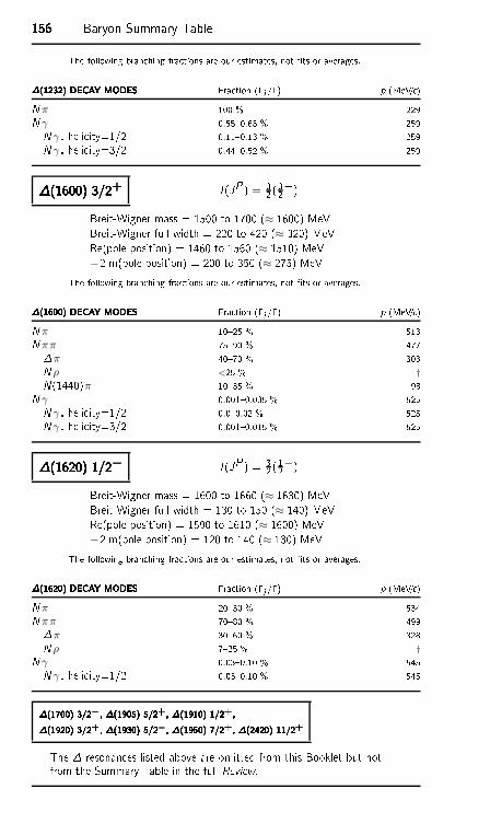
156156156156 Baryon Summary TableThe following bran hing fra tions are our estimates, not ts or averages.(1232) DECAY MODES(1232) DECAY MODES(1232) DECAY MODES(1232) DECAY MODES Fra tion (i /) p (MeV/ )N π 100 % 229N γ 0.550.65 % 259N γ , heli ity=1/2 0.110.13 % 259N γ , heli ity=3/2 0.440.52 % 259(1600) 3/2+(1600) 3/2+(1600) 3/2+(1600) 3/2+ I (JP ) = 32 (32+)Breit-Wigner mass = 1500 to 1700 (≈ 1600) MeVBreit-Wigner full width = 220 to 420 (≈ 320) MeVRe(pole position) = 1460 to 1560 (≈ 1510) MeV−2Im(pole position) = 200 to 350 (≈ 275) MeVThe following bran hing fra tions are our estimates, not ts or averages.(1600) DECAY MODES(1600) DECAY MODES(1600) DECAY MODES(1600) DECAY MODES Fra tion (i /) p (MeV/ )N π 1025 % 513N ππ 7590 % 477π 4070 % 303N ρ <25 % †N(1440)π 1035 % 98N γ 0.0010.035 % 525N γ , heli ity=1/2 0.00.02 % 525N γ , heli ity=3/2 0.0010.015 % 525(1620) 1/2−(1620) 1/2−(1620) 1/2−(1620) 1/2− I (JP ) = 32 (12−)Breit-Wigner mass = 1600 to 1660 (≈ 1630) MeVBreit-Wigner full width = 130 to 150 (≈ 140) MeVRe(pole position) = 1590 to 1610 (≈ 1600) MeV−2Im(pole position) = 120 to 140 (≈ 130) MeVThe following bran hing fra tions are our estimates, not ts or averages.(1620) DECAY MODES(1620) DECAY MODES(1620) DECAY MODES(1620) DECAY MODES Fra tion (i /) p (MeV/ )N π 2030 % 534N ππ 7080 % 499π 3060 % 328N ρ 725 % †N γ 0.030.10 % 545N γ , heli ity=1/2 0.030.10 % 545(1700) 3/2−, (1905) 5/2+, (1910) 1/2+,(1700) 3/2−, (1905) 5/2+, (1910) 1/2+,(1700) 3/2−, (1905) 5/2+, (1910) 1/2+,(1700) 3/2−, (1905) 5/2+, (1910) 1/2+,(1920) 3/2+, (1930) 5/2−, (1950) 7/2+, (2420) 11/2+(1920) 3/2+, (1930) 5/2−, (1950) 7/2+, (2420) 11/2+(1920) 3/2+, (1930) 5/2−, (1950) 7/2+, (2420) 11/2+(1920) 3/2+, (1930) 5/2−, (1950) 7/2+, (2420) 11/2+The resonan es listed above are omitted from this Booklet but notfrom the Summary Table in the full Review.
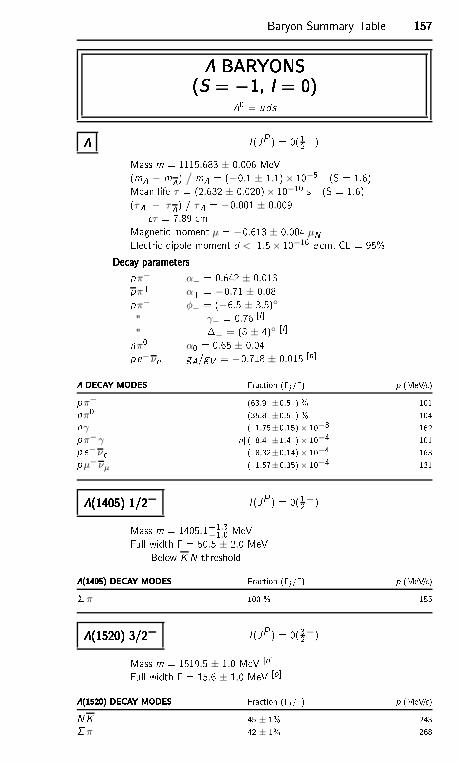
Baryon Summary Table 157157157157 BARYONS BARYONS BARYONS BARYONS(S = −1, I = 0)(S = −1, I = 0)(S = −1, I = 0)(S = −1, I = 0)0 = uds I (JP ) = 0(12+)Mass m = 1115.683 ± 0.006 MeV(m − m) / m = (−0.1 ± 1.1)× 10−5 (S = 1.6)Mean life τ = (2.632 ± 0.020)× 10−10 s (S = 1.6)(τ − τ ) / τ = −0.001 ± 0.009 τ = 7.89 mMagneti moment µ = −0.613 ± 0.004 µNEle tri dipole moment d < 1.5× 10⁻¹⁶ e m, CL = 95%De ay parametersDe ay parametersDe ay parametersDe ay parameterspπ− α− = 0.642 ± 0.013pπ+ α+ = −0.71 ± 0.08pπ− φ− = (−6.5 ± 3.5)" γ− = 0.76 [l" − = (8 ± 4) [lnπ0 α0 = 0.65 ± 0.04p e−νe gA/gV = −0.718 ± 0.015 [h DECAY MODES DECAY MODES DECAY MODES DECAY MODES Fra tion (i /) p (MeV/ )pπ− (63.9 ±0.5 ) % 101nπ0 (35.8 ±0.5 ) % 104nγ ( 1.75±0.15)× 10−3 162pπ− γ [n ( 8.4 ±1.4 )× 10−4 101p e−νe ( 8.32±0.14)× 10−4 163pµ−νµ ( 1.57±0.35)× 10−4 131(1405) 1/2−(1405) 1/2−(1405) 1/2−(1405) 1/2− I (JP ) = 0(12−)Mass m = 1405.1+1.3
−1.0 MeVFull width = 50.5 ± 2.0 MeVBelow K N threshold(1405) DECAY MODES(1405) DECAY MODES(1405) DECAY MODES(1405) DECAY MODES Fra tion (i /) p (MeV/ ) π 100 % 155(1520) 3/2−(1520) 3/2−(1520) 3/2−(1520) 3/2− I (JP ) = 0(32−)Mass m = 1519.5 ± 1.0 MeV [oFull width = 15.6 ± 1.0 MeV [o(1520) DECAY MODES(1520) DECAY MODES(1520) DECAY MODES(1520) DECAY MODES Fra tion (i /) p (MeV/ )NK 45 ± 1% 243 π 42 ± 1% 268
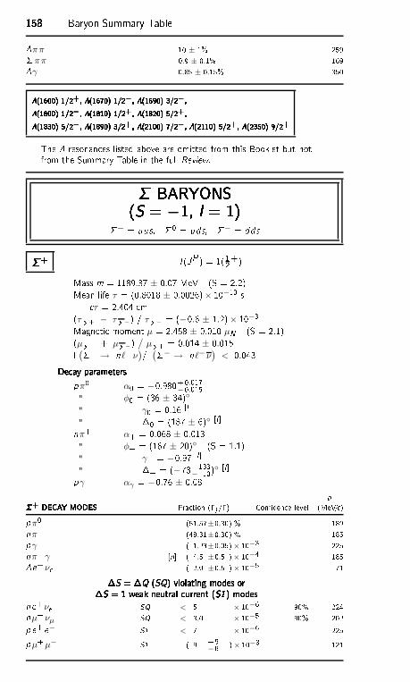
158158158158 Baryon Summary Tableππ 10 ± 1% 259 ππ 0.9 ± 0.1% 169γ 0.85 ± 0.15% 350(1600) 1/2+, (1670) 1/2−, (1690) 3/2−,(1600) 1/2+, (1670) 1/2−, (1690) 3/2−,(1600) 1/2+, (1670) 1/2−, (1690) 3/2−,(1600) 1/2+, (1670) 1/2−, (1690) 3/2−,(1800) 1/2−, (1810) 1/2+, (1820) 5/2+,(1800) 1/2−, (1810) 1/2+, (1820) 5/2+,(1800) 1/2−, (1810) 1/2+, (1820) 5/2+,(1800) 1/2−, (1810) 1/2+, (1820) 5/2+,(1830) 5/2−, (1890) 3/2+, (2100) 7/2−, (2110) 5/2+, (2350) 9/2+(1830) 5/2−, (1890) 3/2+, (2100) 7/2−, (2110) 5/2+, (2350) 9/2+(1830) 5/2−, (1890) 3/2+, (2100) 7/2−, (2110) 5/2+, (2350) 9/2+(1830) 5/2−, (1890) 3/2+, (2100) 7/2−, (2110) 5/2+, (2350) 9/2+The resonan es listed above are omitted from this Booklet but notfrom the Summary Table in the full Review. BARYONS BARYONS BARYONS BARYONS(S = −1, I = 1)(S = −1, I = 1)(S = −1, I = 1)(S = −1, I = 1)+ = uus, 0 = uds, − = dds++++ I (JP ) = 1(12+)Mass m = 1189.37 ± 0.07 MeV (S = 2.2)Mean life τ = (0.8018 ± 0.0026)× 10−10 s τ = 2.404 m(τ+ − τ−) / τ+ = (−0.6 ± 1.2)× 10−3Magneti moment µ = 2.458 ± 0.010 µN (S = 2.1)(µ+ + µ−) /
µ+ = 0.014 ± 0.015(+ → nℓ+ν)/(− → nℓ−ν
)
< 0.043De ay parametersDe ay parametersDe ay parametersDe ay parameterspπ0 α0 = −0.980+0.017−0.015
" φ0 = (36 ± 34)" γ0 = 0.16 [l" 0 = (187 ± 6) [lnπ+ α+ = 0.068 ± 0.013" φ+ = (167 ± 20) (S = 1.1)" γ+ = −0.97 [l" + = (−73+133
− 10) [lpγ αγ = −0.76 ± 0.08 p+ DECAY MODES+ DECAY MODES+ DECAY MODES+ DECAY MODES Fra tion (i /) Conden e level (MeV/ )pπ0 (51.57±0.30) % 189nπ+ (48.31±0.30) % 185pγ ( 1.23±0.05)× 10−3 225nπ+ γ [n ( 4.5 ±0.5 )× 10−4 185e+ νe ( 2.0 ±0.5 )× 10−5 71S = Q (SQ) violating modes orS = Q (SQ) violating modes orS = Q (SQ) violating modes orS = Q (SQ) violating modes orS = 1 weak neutral urrent (S1) modesS = 1 weak neutral urrent (S1) modesS = 1 weak neutral urrent (S1) modesS = 1 weak neutral urrent (S1) modesne+ νe SQ < 5 × 10⁻⁶ 90% 224nµ+ νµ SQ < 3.0 × 10⁻⁵ 90% 202p e+ e− S1 < 7 × 10⁻⁶ 225pµ+µ− S1 ( 9 +9−8 )× 10−8 121
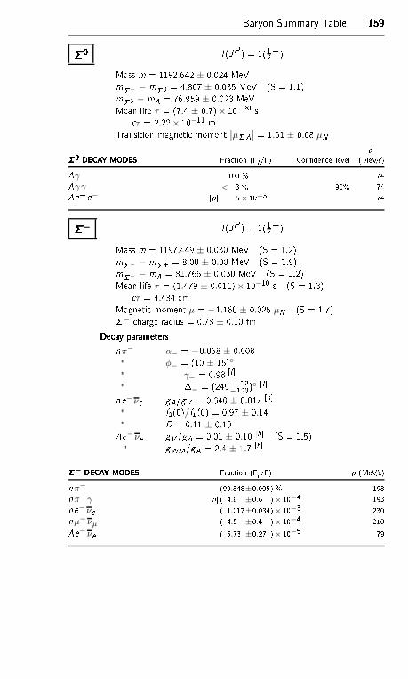
Baryon Summary Table 159159159159 0 0 0 0 I (JP ) = 1(12+)Mass m = 1192.642 ± 0.024 MeVm− − m0 = 4.807 ± 0.035 MeV (S = 1.1)m0 − m = 76.959 ± 0.023 MeVMean life τ = (7.4 ± 0.7)× 10−20 s τ = 2.22× 10⁻¹¹ mTransition magneti moment ∣
∣µ ∣
∣ = 1.61 ± 0.08 µN p0 DECAY MODES0 DECAY MODES0 DECAY MODES0 DECAY MODES Fra tion (i /) Conden e level (MeV/ )γ 100 % 74γ γ < 3 % 90% 74e+ e− [p 5× 10⁻³ 74−−−− I (JP ) = 1(12+)Mass m = 1197.449 ± 0.030 MeV (S = 1.2)m− − m+ = 8.08 ± 0.08 MeV (S = 1.9)m− − m = 81.766 ± 0.030 MeV (S = 1.2)Mean life τ = (1.479 ± 0.011)× 10−10 s (S = 1.3) τ = 4.434 mMagneti moment µ = −1.160 ± 0.025 µN (S = 1.7)− harge radius = 0.78 ± 0.10 fmDe ay parametersDe ay parametersDe ay parametersDe ay parametersnπ− α− = −0.068 ± 0.008" φ− = (10 ± 15)" γ− = 0.98 [l" − = (249+ 12
−120) [lne−νe gA/gV = 0.340 ± 0.017 [h" f2(0)/f1(0) = 0.97 ± 0.14" D = 0.11 ± 0.10e−νe gV /gA = 0.01 ± 0.10 [h (S = 1.5)" gWM/gA = 2.4 ± 1.7 [h− DECAY MODES− DECAY MODES− DECAY MODES− DECAY MODES Fra tion (i /) p (MeV/ )nπ− (99.848±0.005) % 193nπ− γ [n ( 4.6 ±0.6 )× 10−4 193ne− νe ( 1.017±0.034)× 10−3 230nµ− νµ ( 4.5 ±0.4 )× 10−4 210e− νe ( 5.73 ±0.27 )× 10−5 79
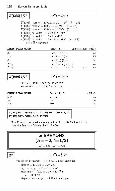
160160160160 Baryon Summary Table (1385) 3/2+ (1385) 3/2+ (1385) 3/2+ (1385) 3/2+ I (JP ) = 1(32+) (1385)+mass m = 1382.80 ± 0.35 MeV (S = 1.9) (1385)0 mass m = 1383.7 ± 1.0 MeV (S = 1.4) (1385)−mass m = 1387.2 ± 0.5 MeV (S = 2.2) (1385)+full width = 36.0 ± 0.7 MeV (1385)0 full width = 36 ± 5 MeV (1385)−full width = 39.4 ± 2.1 MeV (S = 1.7)Below K N threshold p(1385) DECAY MODES(1385) DECAY MODES(1385) DECAY MODES(1385) DECAY MODES Fra tion (i /) Conden e level (MeV/ )π (87.0 ±1.5 ) % 208 π (11.7 ±1.5 ) % 129γ ( 1.25+0.13−0.12) % 241+γ ( 7.0 ±1.7 )× 10−3 180−γ < 2.4 × 10⁻⁴ 90% 173 (1660) 1/2+ (1660) 1/2+ (1660) 1/2+ (1660) 1/2+ I (JP ) = 1(12+)Mass m = 1630 to 1690 (≈ 1660) MeVFull width = 40 to 200 (≈ 100) MeV(1660) DECAY MODES(1660) DECAY MODES(1660) DECAY MODES(1660) DECAY MODES Fra tion (i /) p (MeV/ )NK 1030 % 405π seen 440 π seen 387(1670) 3/2−, (1750) 1/2−, (1775) 5/2−, (1915) 5/2+,(1670) 3/2−, (1750) 1/2−, (1775) 5/2−, (1915) 5/2+,(1670) 3/2−, (1750) 1/2−, (1775) 5/2−, (1915) 5/2+,(1670) 3/2−, (1750) 1/2−, (1775) 5/2−, (1915) 5/2+,(1940) 3/2−, (2030) 7/2+, (2250)(1940) 3/2−, (2030) 7/2+, (2250)(1940) 3/2−, (2030) 7/2+, (2250)(1940) 3/2−, (2030) 7/2+, (2250)The resonan es listed above are omitted from this Booklet but notfrom the Summary Table in the full Review. BARYONS BARYONS BARYONS BARYONS(S=−2, I=1/2)(S=−2, I=1/2)(S=−2, I=1/2)(S=−2, I=1/2) 0 = uss, − = dss 0 0 0 0 I (JP ) = 12 (12+)P is not yet measured; + is the quark model predi tion.Mass m = 1314.86 ± 0.20 MeVm− − m0 = 6.85 ± 0.21 MeVMean life τ = (2.90 ± 0.09)× 10−10 s τ = 8.71 mMagneti moment µ = −1.250 ± 0.014 µN
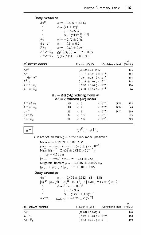
Baryon Summary Table 161161161161De ay parametersDe ay parametersDe ay parametersDe ay parametersπ0 α = −0.406 ± 0.013" φ = (21 ± 12)" γ = 0.85 [l" = (218+12
−19) [lγ α = −0.70 ± 0.07e+ e− α = −0.8 ± 0.20γ α = −0.69 ± 0.06+ e−νe g1(0)/f1(0) = 1.22 ± 0.05+ e−νe f2(0)/f1(0) = 2.0 ± 0.9 p0 DECAY MODES0 DECAY MODES0 DECAY MODES0 DECAY MODES Fra tion (i /) Conden e level (MeV/ )π0 (99.524±0.012) % 135γ ( 1.17 ±0.07 )× 10−3 184e+ e− ( 7.6 ±0.6 )× 10−6 1840 γ ( 3.33 ±0.10 )× 10−3 117+ e− νe ( 2.52 ±0.08 )× 10−4 120+µ− νµ ( 2.33 ±0.35 )× 10−6 64S = Q (SQ) violating modes orS = Q (SQ) violating modes orS = Q (SQ) violating modes orS = Q (SQ) violating modes orS = 2 forbidden (S2) modesS = 2 forbidden (S2) modesS = 2 forbidden (S2) modesS = 2 forbidden (S2) modes− e+ νe SQ < 9 × 10⁻⁴ 90% 112−µ+ νµ SQ < 9 × 10⁻⁴ 90% 49pπ− S2 < 8 × 10⁻⁶ 90% 299p e−νe S2 < 1.3 × 10⁻³ 323pµ−νµ S2 < 1.3 × 10⁻³ 309−−−− I (JP ) = 12 (12+)P is not yet measured; + is the quark model predi tion.Mass m = 1321.71 ± 0.07 MeV(m− − m+) / m− = (−3 ± 9)× 10−5Mean life τ = (1.639 ± 0.015)× 10−10 s τ = 4.91 m(τ− − τ +) / τ− = −0.01 ± 0.07Magneti moment µ = −0.6507 ± 0.0025 µN(µ− + µ+) / ∣
∣µ−
∣
∣ = +0.01 ± 0.05De ay parametersDe ay parametersDe ay parametersDe ay parametersπ− α = −0.458 ± 0.012 (S = 1.8)[α(−)α−() − α(+)α+() / [ sum = (0 ± 7)× 10−4" φ = (−2.1 ± 0.8)" γ = 0.89 [l" = (175.9 ± 1.5) [le−νe gA/gV = −0.25 ± 0.05 [h p− DECAY MODES− DECAY MODES− DECAY MODES− DECAY MODES Fra tion (i /) Conden e level (MeV/ )π− (99.887±0.035) % 140−γ ( 1.27 ±0.23 )× 10−4 118e− νe ( 5.63 ±0.31 )× 10−4 190
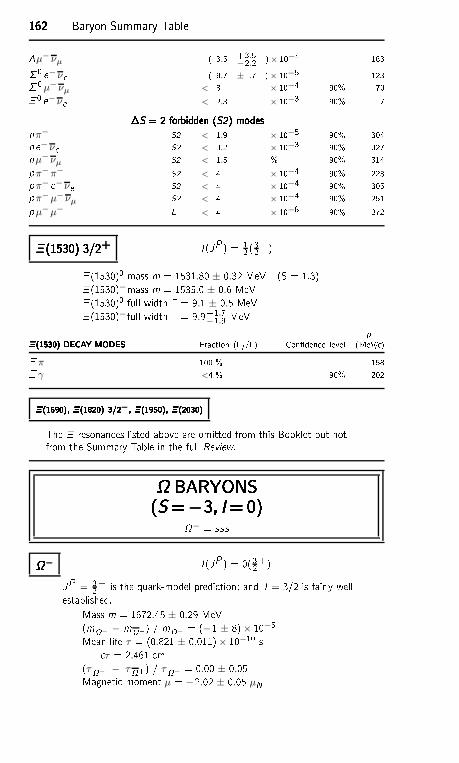
162162162162 Baryon Summary Tableµ− νµ ( 3.5 +3.5−2.2 )× 10−4 1630 e−νe ( 8.7 ±1.7 )× 10−5 1230µ−νµ < 8 × 10⁻⁴ 90% 70 0 e−νe < 2.3 × 10⁻³ 90% 7S = 2 forbidden (S2) modesS = 2 forbidden (S2) modesS = 2 forbidden (S2) modesS = 2 forbidden (S2) modesnπ− S2 < 1.9 × 10⁻⁵ 90% 304ne− νe S2 < 3.2 × 10⁻³ 90% 327nµ− νµ S2 < 1.5 % 90% 314pπ−π− S2 < 4 × 10⁻⁴ 90% 223pπ− e−νe S2 < 4 × 10⁻⁴ 90% 305pπ−µ−νµ S2 < 4 × 10⁻⁴ 90% 251pµ−µ− L < 4 × 10⁻⁸ 90% 272 (1530) 3/2+ (1530) 3/2+ (1530) 3/2+ (1530) 3/2+ I (JP ) = 12 (32+) (1530)0 mass m = 1531.80 ± 0.32 MeV (S = 1.3) (1530)−mass m = 1535.0 ± 0.6 MeV (1530)0 full width = 9.1 ± 0.5 MeV (1530)− full width = 9.9+1.7
−1.9 MeV p(1530) DECAY MODES(1530) DECAY MODES(1530) DECAY MODES(1530) DECAY MODES Fra tion (i /) Conden e level (MeV/ ) π 100 % 158 γ <4 % 90% 202(1690), (1820) 3/2−, (1950), (2030)(1690), (1820) 3/2−, (1950), (2030)(1690), (1820) 3/2−, (1950), (2030)(1690), (1820) 3/2−, (1950), (2030)The resonan es listed above are omitted from this Booklet but notfrom the Summary Table in the full Review. BARYONS BARYONS BARYONS BARYONS(S=−3, I=0)(S=−3, I=0)(S=−3, I=0)(S=−3, I=0)− = sss−−−− I (JP ) = 0(32+)JP = 32+ is the quark-model predi tion; and J = 3/2 is fairly wellestablished.Mass m = 1672.45 ± 0.29 MeV(m− − m+) / m− = (−1 ± 8)× 10−5Mean life τ = (0.821 ± 0.011)× 10−10 s τ = 2.461 m(τ− − τ+) / τ− = 0.00 ± 0.05Magneti moment µ = −2.02 ± 0.05 µN
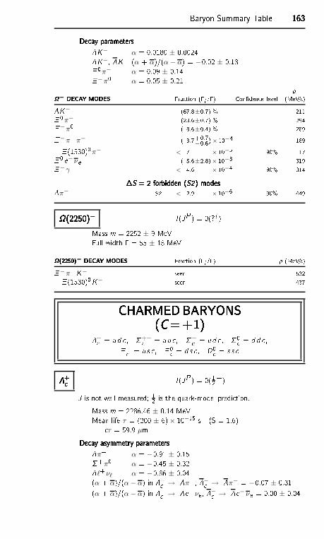
Baryon Summary Table 163163163163De ay parametersDe ay parametersDe ay parametersDe ay parametersK− α = 0.0180 ± 0.0024K−, K+ (α + α)/(α − α) = −0.02 ± 0.13 0π− α = 0.09 ± 0.14−π0 α = 0.05 ± 0.21 p− DECAY MODES− DECAY MODES− DECAY MODES− DECAY MODES Fra tion (i /) Conden e level (MeV/ )K− (67.8±0.7) % 211 0π− (23.6±0.7) % 294−π0 ( 8.6±0.4) % 289−π+π− ( 3.7+0.7−0.6)× 10−4 189 (1530)0π− < 7 × 10⁻⁵ 90% 17 0 e−νe ( 5.6±2.8)× 10−3 319−γ < 4.6 × 10⁻⁴ 90% 314S = 2 forbidden (S2) modesS = 2 forbidden (S2) modesS = 2 forbidden (S2) modesS = 2 forbidden (S2) modesπ− S2 < 2.9 × 10⁻⁶ 90% 449(2250)−(2250)−(2250)−(2250)− I (JP ) = 0(??)Mass m = 2252 ± 9 MeVFull width = 55 ± 18 MeV(2250)− DECAY MODES(2250)− DECAY MODES(2250)− DECAY MODES(2250)− DECAY MODES Fra tion (i /) p (MeV/ )−π+K− seen 532 (1530)0K− seen 437CHARMEDBARYONSCHARMEDBARYONSCHARMEDBARYONSCHARMEDBARYONS(C=+1)(C=+1)(C=+1)(C=+1)+ = ud , ++ = uu , + = ud , 0 = d d ,+ = u s , 0 = d s , 0 = s s + + + + I (JP ) = 0(12+)J is not well measured; 12 is the quark-model predi tion.Mass m = 2286.46 ± 0.14 MeVMean life τ = (200 ± 6)× 10−15 s (S = 1.6) τ = 59.9 µmDe ay asymmetry parametersDe ay asymmetry parametersDe ay asymmetry parametersDe ay asymmetry parametersπ+ α = −0.91 ± 0.15+π0 α = −0.45 ± 0.32ℓ+νℓ α = −0.86 ± 0.04(α + α)/(α − α) in + → π+, − → π− = −0.07 ± 0.31(α + α)/(α − α) in + → e+ νe , − → e− νe = 0.00 ± 0.04
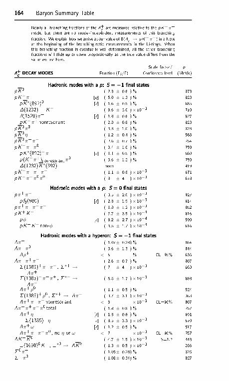
164164164164 Baryon Summary TableNearly all bran hing fra tions of the + are measured relative to the pK−π+mode, but there are no model-independent measurements of this bran hingfra tion. We explain how we arrive at our value of B(+ → pK−π+) in a Noteat the beginning of the bran hing-ratio measurements in the Listings. Whenthis bran hing fra tion is eventually well determined, all the other bran hingfra tions will slide up or down proportionally as the true value diers from thevalue we use here. S ale fa tor/ p+ DECAY MODES+ DECAY MODES+ DECAY MODES+ DECAY MODES Fra tion (i /) Conden e level (MeV/ )Hadroni modes with a p: S = −1 nal statesHadroni modes with a p: S = −1 nal statesHadroni modes with a p: S = −1 nal statesHadroni modes with a p: S = −1 nal statespK0 ( 2.3 ± 0.6 ) % 873pK−π+ [q ( 5.0 ± 1.3 ) % 823pK∗(892)0 [r ( 1.6 ± 0.5 ) % 685(1232)++K− ( 8.6 ± 3.0 )× 10−3 710(1520)π+ [r ( 1.8 ± 0.6 ) % 627pK−π+nonresonant ( 2.8 ± 0.8 ) % 823pK0π0 ( 3.3 ± 1.0 ) % 823pK0η ( 1.2 ± 0.4 ) % 568pK0π+π− ( 2.6 ± 0.7 ) % 754pK−π+π0 ( 3.4 ± 1.0 ) % 759pK∗(892)−π+ [r ( 1.1 ± 0.5 ) % 580p (K−π+)nonresonant π0 ( 3.6 ± 1.2 ) % 759(1232)K∗(892) seen 419pK−π+π+π− ( 1.1 ± 0.8 )× 10−3 671pK−π+π0π0 ( 8 ± 4 )× 10−3 678Hadroni modes with a p: S = 0 nal statesHadroni modes with a p: S = 0 nal statesHadroni modes with a p: S = 0 nal statesHadroni modes with a p: S = 0 nal statespπ+π− ( 3.5 ± 2.0 )× 10−3 927p f0(980) [r ( 2.8 ± 1.9 )× 10−3 614pπ+π+π−π− ( 1.8 ± 1.2 )× 10−3 852pK+K− ( 7.7 ± 3.5 )× 10−4 616pφ [r ( 8.2 ± 2.7 )× 10−4 590pK+K−non-φ ( 3.5 ± 1.7 )× 10−4 616Hadroni modes with a hyperon: S = −1 nal statesHadroni modes with a hyperon: S = −1 nal statesHadroni modes with a hyperon: S = −1 nal statesHadroni modes with a hyperon: S = −1 nal statesπ+ ( 1.07± 0.28) % 864π+π0 ( 3.6 ± 1.3 ) % 844ρ+ < 5 % CL=95% 636π+π+π− ( 2.6 ± 0.7 ) % 807 (1385)+π+π− , ∗+ →π+ ( 7 ± 4 )× 10−3 688 (1385)−π+π+ , ∗− →π−( 5.5 ± 1.7 )× 10−3 688π+ ρ0 ( 1.1 ± 0.5 ) % 524 (1385)+ρ0 , ∗+ → π+ ( 3.7 ± 3.1 )× 10−3 363π+π+π− nonresonant < 8 × 10⁻³ CL=90% 807π+π+π−π0 total ( 1.8 ± 0.8 ) % 757π+ η [r ( 1.8 ± 0.6 ) % 691 (1385)+η [r ( 8.5 ± 3.3 )× 10−3 570π+ω [r ( 1.2 ± 0.5 ) % 517π+π+π−π0 , no η or ω < 7 × 10⁻³ CL=90% 757K+K0 ( 4.7 ± 1.5 )× 10−3 S=1.2 443 (1690)0K+ , ∗0 → K0 ( 1.3 ± 0.5 )× 10−3 2860π+ ( 1.05± 0.28) % 825+π0 ( 1.00± 0.34) % 827
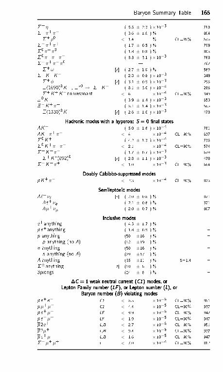
Baryon Summary Table 165165165165+η ( 5.5 ± 2.3 )× 10−3 713+π+π− ( 3.6 ± 1.0 ) % 804+ρ0 < 1.4 % CL=95% 575−π+π+ ( 1.7 ± 0.5 ) % 7990π+π0 ( 1.8 ± 0.8 ) % 8030π+π+π− ( 8.3 ± 3.1 )× 10−3 763+π+π−π0 | 767+ω [r ( 2.7 ± 1.0 ) % 569+K+K− ( 2.8 ± 0.8 )× 10−3 349+φ [r ( 3.1 ± 0.9 )× 10−3 295 (1690)0K+ , ∗0 → +K− ( 8.1 ± 3.0 )× 10−4 286+K+K−nonresonant < 6 × 10⁻⁴ CL=90% 349 0K+ ( 3.9 ± 1.4 )× 10−3 653−K+π+ ( 5.1 ± 1.4 )× 10−3 565 (1530)0K+ [r ( 2.6 ± 1.0 )× 10−3 473Hadroni modes with a hyperon: S = 0 nal statesHadroni modes with a hyperon: S = 0 nal statesHadroni modes with a hyperon: S = 0 nal statesHadroni modes with a hyperon: S = 0 nal statesK+ ( 5.0 ± 1.6 )× 10−4 781K+π+π− < 4 × 10⁻⁴ CL=90% 6370K+ ( 4.2 ± 1.3 )× 10−4 7350K+π+π− < 2.1 × 10⁻⁴ CL=90% 574+K+π− ( 1.7 ± 0.7 )× 10−3 670+K∗(892)0 [r ( 2.8 ± 1.1 )× 10−3 470−K+π+ < 1.0 × 10⁻³ CL=90% 664Doubly Cabibbo-suppressed modesDoubly Cabibbo-suppressed modesDoubly Cabibbo-suppressed modesDoubly Cabibbo-suppressed modespK+π− < 2.3 × 10⁻⁴ CL=90% 823Semileptoni modesSemileptoni modesSemileptoni modesSemileptoni modesℓ+νℓ [s ( 2.0 ± 0.6 ) % 871e+ νe ( 2.1 ± 0.6 ) % 871µ+ νµ ( 2.0 ± 0.7 ) % 867In lusive modesIn lusive modesIn lusive modesIn lusive modese+ anything ( 4.5 ± 1.7 ) % p e+anything ( 1.8 ± 0.9 ) % p anything (50 ±16 ) % p anything (no ) (12 ±19 ) % n anything (50 ±16 ) % n anything (no ) (29 ±17 ) % anything (35 ±11 ) % S=1.4 ± anything [t (10 ± 5 ) % 3prongs (24 ± 8 ) % C = 1 weak neutral urrent (C1) modes, orC = 1 weak neutral urrent (C1) modes, orC = 1 weak neutral urrent (C1) modes, orC = 1 weak neutral urrent (C1) modes, orLepton Family number (LF ), or Lepton number (L), orLepton Family number (LF ), or Lepton number (L), orLepton Family number (LF ), or Lepton number (L), orLepton Family number (LF ), or Lepton number (L), orBaryon number (B) violating modesBaryon number (B) violating modesBaryon number (B) violating modesBaryon number (B) violating modesp e+ e− C1 < 5.5 × 10⁻⁶ CL=90% 951pµ+µ− C1 < 4.4 × 10⁻⁵ CL=90% 937p e+µ− LF < 9.9 × 10⁻⁶ CL=90% 947p e−µ+ LF < 1.9 × 10⁻⁵ CL=90% 947p2e+ L,B < 2.7 × 10⁻⁶ CL=90% 951p2µ+ L,B < 9.4 × 10⁻⁶ CL=90% 937p e+µ+ L,B < 1.6 × 10⁻⁵ CL=90% 947−µ+µ+ L < 7.0 × 10⁻⁴ CL=90% 812
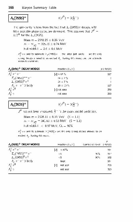
166166166166 Baryon Summary Table (2595)+ (2595)+ (2595)+ (2595)+ I (JP ) = 0(12−)The spin-parity follows from the fa t that (2455)π de ays, withlittle available phase spa e, are dominant. This assumes that JP =1/2+ for the (2455).Mass m = 2592.25 ± 0.28 MeVm − m+ = 305.79 ± 0.24 MeVFull width = 2.6 ± 0.6 MeV+ ππ and its submode (2455)π | the latter just barely | are the onlystrong de ays allowed to an ex ited + having this mass; and the submodeseems to dominate. (2595)+ DECAY MODES (2595)+ DECAY MODES (2595)+ DECAY MODES (2595)+ DECAY MODES Fra tion (i /) p (MeV/ )+ π+π− [u≈ 67 % 117 (2455)++π− 24 ± 7 % † (2455)0π+ 24 ± 7 % †+ π+π−3-body 18 ± 10 % 117+ π0 [v not seen 258+ γ not seen 288 (2625)+ (2625)+ (2625)+ (2625)+ I (JP ) = 0(32−)JP has not been measured; 32− is the quark-model predi tion.Mass m = 2628.11 ± 0.19 MeV (S = 1.1)m − m+ = 341.65 ± 0.13 MeV (S = 1.1)Full width < 0.97 MeV, CL = 90%+ ππ and its submode (2455)π are the only strong de ays allowed to anex ited + having this mass. p (2625)+ DECAY MODES (2625)+ DECAY MODES (2625)+ DECAY MODES (2625)+ DECAY MODES Fra tion (i /) Conden e level (MeV/ )+ π+π− [u ≈ 67% 184 (2455)++π− <5 90% 102 (2455)0π+ <5 90% 102+ π+π−3-body large 184+ π0 [v not seen 293+ γ not seen 319
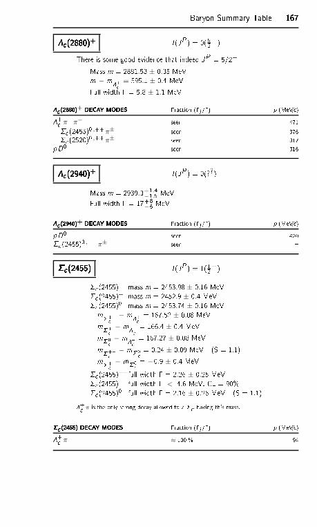
Baryon Summary Table 167167167167 (2880)+ (2880)+ (2880)+ (2880)+ I (JP ) = 0(52+)There is some good eviden e that indeed JP = 5/2+Mass m = 2881.53 ± 0.35 MeVm − m+ = 595.1 ± 0.4 MeVFull width = 5.8 ± 1.1 MeV (2880)+ DECAY MODES (2880)+ DECAY MODES (2880)+ DECAY MODES (2880)+ DECAY MODES Fra tion (i /) p (MeV/ )+ π+π− seen 471 (2455)0 ,++π± seen 376 (2520)0 ,++π± seen 317pD0 seen 316 (2940)+ (2940)+ (2940)+ (2940)+ I (JP ) = 0(??)Mass m = 2939.3+1.4−1.5 MeVFull width = 17+8−6 MeV (2940)+ DECAY MODES (2940)+ DECAY MODES (2940)+ DECAY MODES (2940)+ DECAY MODES Fra tion (i /) p (MeV/ )pD0 seen 420 (2455)0 ,++π± seen (2455) (2455) (2455) (2455) I (JP ) = 1(12+) (2455)++mass m = 2453.98 ± 0.16 MeV (2455)+ mass m = 2452.9 ± 0.4 MeV (2455)0 mass m = 2453.74 ± 0.16 MeVm++ − m+ = 167.52 ± 0.08 MeVm+ − m+ = 166.4 ± 0.4 MeVm0 − m+ = 167.27 ± 0.08 MeVm++ − m0 = 0.24 ± 0.09 MeV (S = 1.1)m+ − m0 = −0.9 ± 0.4 MeV (2455)++full width = 2.26 ± 0.25 MeV (2455)+ full width < 4.6 MeV, CL = 90% (2455)0 full width = 2.16 ± 0.26 MeV (S = 1.1)+ π is the only strong de ay allowed to a having this mass. (2455) DECAY MODES (2455) DECAY MODES (2455) DECAY MODES (2455) DECAY MODES Fra tion (i /) p (MeV/ )+ π ≈ 100 % 94
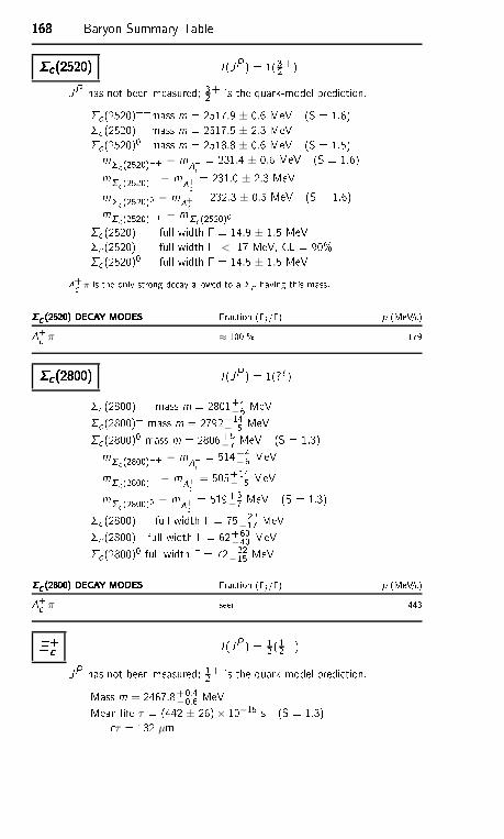
168168168168 Baryon Summary Table (2520) (2520) (2520) (2520) I (JP ) = 1(32+)JP has not been measured; 32+ is the quark-model predi tion. (2520)++mass m = 2517.9 ± 0.6 MeV (S = 1.6) (2520)+ mass m = 2517.5 ± 2.3 MeV (2520)0 mass m = 2518.8 ± 0.6 MeV (S = 1.5)m (2520)++ − m+ = 231.4 ± 0.6 MeV (S = 1.6)m (2520)+ − m+ = 231.0 ± 2.3 MeVm (2520)0 − m+ = 232.3 ± 0.5 MeV (S = 1.6)m (2520)++ − m (2520)0 (2520)++ full width = 14.9 ± 1.5 MeV (2520)+ full width < 17 MeV, CL = 90% (2520)0 full width = 14.5 ± 1.5 MeV+ π is the only strong de ay allowed to a having this mass. (2520) DECAY MODES (2520) DECAY MODES (2520) DECAY MODES (2520) DECAY MODES Fra tion (i /) p (MeV/ )+ π ≈ 100 % 179 (2800) (2800) (2800) (2800) I (JP ) = 1(??) (2800)++ mass m = 2801+4−6 MeV (2800)+ mass m = 2792+14
− 5 MeV (2800)0 mass m = 2806+5−7 MeV (S = 1.3)m (2800)++ − m+ = 514+4
−6 MeVm (2800)+ − m+ = 505+14− 5 MeVm (2800)0 − m+ = 519+5−7 MeV (S = 1.3) (2800)++ full width = 75+22
−17 MeV (2800)+ full width = 62+60−40 MeV (2800)0 full width = 72+22−15 MeV (2800) DECAY MODES (2800) DECAY MODES (2800) DECAY MODES (2800) DECAY MODES Fra tion (i /) p (MeV/ )+ π seen 443+ + + + I (JP ) = 12 (12+)JP has not been measured; 12+ is the quark-model predi tion.Mass m = 2467.8+0.4
−0.6 MeVMean life τ = (442 ± 26)× 10−15 s (S = 1.3) τ = 132 µm
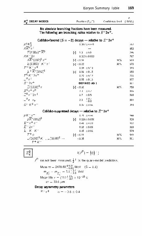
Baryon Summary Table 169169169169p+ DECAY MODES+ DECAY MODES+ DECAY MODES+ DECAY MODES Fra tion (i /) Conden e level (MeV/ )No absolute bran hing fra tions have been measured.No absolute bran hing fra tions have been measured.No absolute bran hing fra tions have been measured.No absolute bran hing fra tions have been measured.The following are bran hing ratios relative to −2π+.The following are bran hing ratios relative to −2π+.The following are bran hing ratios relative to −2π+.The following are bran hing ratios relative to −2π+.Cabibbo-favored (S = −2) de ays | relative to −2π+Cabibbo-favored (S = −2) de ays | relative to −2π+Cabibbo-favored (S = −2) de ays | relative to −2π+Cabibbo-favored (S = −2) de ays | relative to −2π+p2K0S 0.087±0.021 767K0π+ | 852 (1385)+K0 [r 1.0 ±0.5 746K−2π+ 0.323±0.033 787K∗(892)0π+ [r <0.16 90% 608 (1385)+K−π+ [r <0.23 90% 678+K−π+ 0.94 ±0.10 810+K∗(892)0 [r 0.81 ±0.15 6580K−2π+ 0.27 ±0.12 735 0π+ 0.55 ±0.16 877−2π+ DEFINED AS 1DEFINED AS 1DEFINED AS 1DEFINED AS 1 851 (1530)0π+ [r <0.10 90% 750 0π+π0 2.3 ±0.7 856 0π−2π+ 1.7 ±0.5 818 0 e+νe 2.3 +0.7−0.8 884−K+π+ 0.07 ±0.04 399Cabibbo-suppressed de ays | relative to −2π+Cabibbo-suppressed de ays | relative to −2π+Cabibbo-suppressed de ays | relative to −2π+Cabibbo-suppressed de ays | relative to −2π+pK−π+ 0.21 ±0.04 944pK∗(892)0 [r 0.116±0.030 828+π+π− 0.48 ±0.20 922−2π+ 0.18 ±0.09 918+K+K− 0.15 ±0.06 579+φ [r <0.11 90% 549 (1690)0K+ , (1690)0 →+K−
<0.05 90% 501 0 0 0 0 I (JP ) = 12 (12+)JP has not been measured; 12+ is the quark-model predi tion.Mass m = 2470.88+0.34−0.80 MeV (S = 1.1)m0 − m+ = 3.1+0.4
−0.5 MeVMean life τ = (112+13−10)× 10−15 s τ = 33.6 µmDe ay asymmetry parametersDe ay asymmetry parametersDe ay asymmetry parametersDe ay asymmetry parameters−π+ α = −0.6 ± 0.4
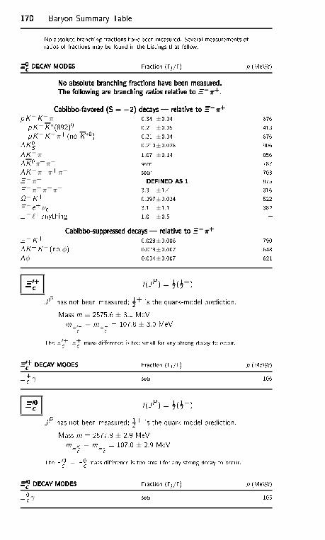
170170170170 Baryon Summary TableNo absolute bran hing fra tions have been measured. Several measurements ofratios of fra tions may be found in the Listings that follow.0 DECAY MODES0 DECAY MODES0 DECAY MODES0 DECAY MODES Fra tion (i /) p (MeV/ )No absolute bran hing fra tions have been measured.No absolute bran hing fra tions have been measured.No absolute bran hing fra tions have been measured.No absolute bran hing fra tions have been measured.The following are bran hing ratios relative to −π+.The following are bran hing ratios relative to −π+.The following are bran hing ratios relative to −π+.The following are bran hing ratios relative to −π+.Cabibbo-favored (S = −2) de ays | relative to −π+Cabibbo-favored (S = −2) de ays | relative to −π+Cabibbo-favored (S = −2) de ays | relative to −π+Cabibbo-favored (S = −2) de ays | relative to −π+pK−K−π+ 0.34 ±0.04 676pK−K∗(892)0 0.21 ±0.05 413pK−K−π+ (no K∗0) 0.21 ±0.04 676K0S 0.210±0.028 906K−π+ 1.07 ±0.14 856K0π+π− seen 787K−π+π+π− seen 703−π+ DEFINED AS 1DEFINED AS 1DEFINED AS 1DEFINED AS 1 875−π+π+π− 3.3 ±1.4 816−K+ 0.297±0.024 522− e+ νe 3.1 ±1.1 882− ℓ+anything 1.0 ±0.5 Cabibbo-suppressed de ays | relative to −π+Cabibbo-suppressed de ays | relative to −π+Cabibbo-suppressed de ays | relative to −π+Cabibbo-suppressed de ays | relative to −π+−K+ 0.028±0.006 790K+K− (no φ) 0.029±0.007 648φ 0.034±0.007 621 ′+ ′+ ′+ ′+ I (JP ) = 12 (12+)JP has not been measured; 12+ is the quark-model predi tion.Mass m = 2575.6 ± 3.1 MeVm ′+ − m+ = 107.8 ± 3.0 MeVThe ′+ + mass dieren e is too small for any strong de ay to o ur. ′+ DECAY MODES ′+ DECAY MODES ′+ DECAY MODES ′+ DECAY MODES Fra tion (i /) p (MeV/ )+ γ seen 106 ′0 ′0 ′0 ′0 I (JP ) = 12 (12+)JP has not been measured; 12+ is the quark-model predi tion.Mass m = 2577.9 ± 2.9 MeVm ′0 − m0 = 107.0 ± 2.9 MeVThe ′0 − 0 mass dieren e is too small for any strong de ay to o ur. ′0 DECAY MODES ′0 DECAY MODES ′0 DECAY MODES ′0 DECAY MODES Fra tion (i /) p (MeV/ ) 0 γ seen 105
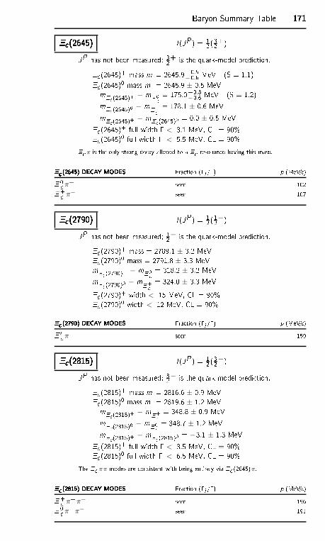
Baryon Summary Table 171171171171 (2645) (2645) (2645) (2645) I (JP ) = 12 (32+)JP has not been measured; 32+ is the quark-model predi tion. (2645)+ mass m = 2645.9+0.5−0.6 MeV (S = 1.1) (2645)0 mass m = 2645.9 ± 0.5 MeVm (2645)+ − m0 = 175.0+0.8−0.6 MeV (S = 1.2)m (2645)0 − m+ = 178.1 ± 0.6 MeVm (2645)+ − m (2645)0 = 0.0 ± 0.5 MeV (2645)+ full width < 3.1 MeV, CL = 90% (2645)0 full width < 5.5 MeV, CL = 90% π is the only strong de ay allowed to a resonan e having this mass. (2645) DECAY MODES (2645) DECAY MODES (2645) DECAY MODES (2645) DECAY MODES Fra tion (i /) p (MeV/ ) 0 π+ seen 102+ π− seen 107 (2790) (2790) (2790) (2790) I (JP ) = 12 (12−)JP has not been measured; 12− is the quark-model predi tion. (2790)+ mass = 2789.1 ± 3.2 MeV (2790)0 mass = 2791.8 ± 3.3 MeVm (2790)+ − m0 = 318.2 ± 3.2 MeVm (2790)0 − m+ = 324.0 ± 3.3 MeV (2790)+ width < 15 MeV, CL = 90% (2790)0 width < 12 MeV, CL = 90% (2790) DECAY MODES (2790) DECAY MODES (2790) DECAY MODES (2790) DECAY MODES Fra tion (i /) p (MeV/ ) ′ π seen 159 (2815) (2815) (2815) (2815) I (JP ) = 12 (32−)JP has not been measured; 32− is the quark-model predi tion. (2815)+ mass m = 2816.6 ± 0.9 MeV (2815)0 mass m = 2819.6 ± 1.2 MeVm (2815)+ − m+ = 348.8 ± 0.9 MeVm (2815)0 − m0 = 348.7 ± 1.2 MeVm (2815)+ − m (2815)0 = −3.1 ± 1.3 MeV (2815)+ full width < 3.5 MeV, CL = 90% (2815)0 full width < 6.5 MeV, CL = 90%The ππ modes are onsistent with being entirely via (2645)π. (2815) DECAY MODES (2815) DECAY MODES (2815) DECAY MODES (2815) DECAY MODES Fra tion (i /) p (MeV/ )+ π+π− seen 196 0 π+π− seen 191
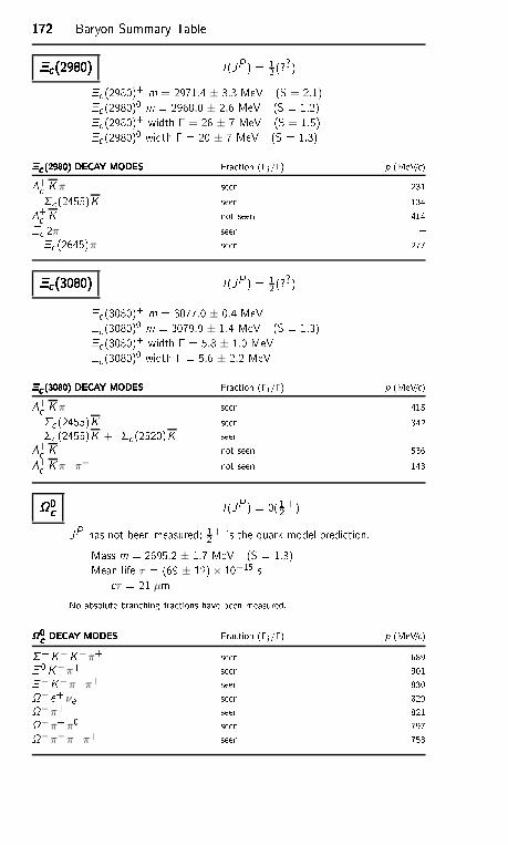
172172172172 Baryon Summary Table (2980) (2980) (2980) (2980) I (JP ) = 12 (??) (2980)+ m = 2971.4 ± 3.3 MeV (S = 2.1) (2980)0 m = 2968.0 ± 2.6 MeV (S = 1.2) (2980)+ width = 26 ± 7 MeV (S = 1.5) (2980)0 width = 20 ± 7 MeV (S = 1.3) (2980) DECAY MODES (2980) DECAY MODES (2980) DECAY MODES (2980) DECAY MODES Fra tion (i /) p (MeV/ )+ K π seen 231 (2455)K seen 134+ K not seen 414 2π seen (2645)π seen 277 (3080) (3080) (3080) (3080) I (JP ) = 12 (??) (3080)+ m = 3077.0 ± 0.4 MeV (3080)0 m = 3079.9 ± 1.4 MeV (S = 1.3) (3080)+ width = 5.8 ± 1.0 MeV (3080)0 width = 5.6 ± 2.2 MeV (3080) DECAY MODES (3080) DECAY MODES (3080) DECAY MODES (3080) DECAY MODES Fra tion (i /) p (MeV/ )+ K π seen 415 (2455)K seen 342 (2455)K + (2520)K seen + K not seen 536+ K π+π− not seen 1430 0 0 0 I (JP ) = 0(12+)JP has not been measured; 12+ is the quark-model predi tion.Mass m = 2695.2 ± 1.7 MeV (S = 1.3)Mean life τ = (69 ± 12)× 10−15 s τ = 21 µmNo absolute bran hing fra tions have been measured.0 DECAY MODES0 DECAY MODES0 DECAY MODES0 DECAY MODES Fra tion (i /) p (MeV/ )+K−K−π+ seen 689 0K−π+ seen 901−K−π+π+ seen 830− e+ νe seen 829−π+ seen 821−π+π0 seen 797−π−π+π+ seen 753
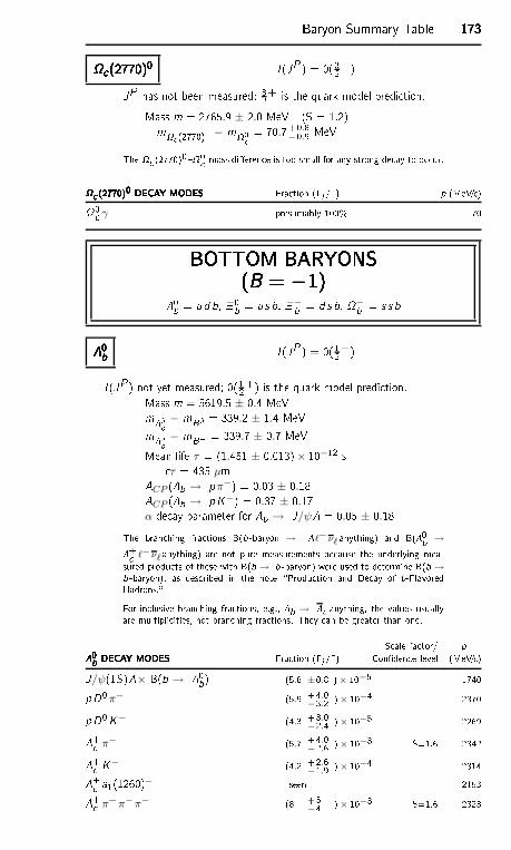
Baryon Summary Table 173173173173 (2770)0 (2770)0 (2770)0 (2770)0 I (JP ) = 0(32+)JP has not been measured; 32+ is the quark-model predi tion.Mass m = 2765.9 ± 2.0 MeV (S = 1.2)m (2770)0 − m0 = 70.7+0.8−0.9 MeVThe (2770)00 mass dieren e is too small for any strong de ay to o ur. (2770)0 DECAY MODES (2770)0 DECAY MODES (2770)0 DECAY MODES (2770)0 DECAY MODES Fra tion (i /) p (MeV/ )0 γ presumably 100% 70BOTTOM BARYONSBOTTOM BARYONSBOTTOM BARYONSBOTTOM BARYONS(B = −1)(B = −1)(B = −1)(B = −1)0b = ud b, 0b = u s b, −b = d s b, −b = s s b0b0b0b0b I (JP ) = 0(12+)I (JP ) not yet measured; 0(12+) is the quark model predi tion.Mass m = 5619.5 ± 0.4 MeVm0b − mB0 = 339.2 ± 1.4 MeVm0b − mB+ = 339.7 ± 0.7 MeVMean life τ = (1.451 ± 0.013)× 10−12 s τ = 435 µmACP (b → pπ−) = 0.03 ± 0.18ACP (b → pK−) = 0.37 ± 0.17
α de ay parameter for b → J/ψ = 0.05 ± 0.18The bran hing fra tions B(b -baryon → ℓ− νℓ anything) and B(0b →+ ℓ− νℓ anything) are not pure measurements be ause the underlying mea-sured produ ts of these with B(b → b -baryon) were used to determine B(b →b -baryon), as des ribed in the note \Produ tion and De ay of b-FlavoredHadrons."For in lusive bran hing fra tions, e.g., b → anything, the values usuallyare multipli ities, not bran hing fra tions. They an be greater than one.S ale fa tor/ p0b DECAY MODES0b DECAY MODES0b DECAY MODES0b DECAY MODES Fra tion (i /) Conden e level (MeV/ )J/ψ(1S)× B(b → 0b) (5.8 ±0.8 )× 10−5 1740pD0π− (5.9 +4.0−3.2 ) × 10−4 2370pD0K− (4.3 +3.0−2.4 ) × 10−5 2269+ π− (5.7 +4.0−2.6 ) × 10−3 S=1.6 2342+ K− (4.2 +2.6−1.9 ) × 10−4 2314+ a1(1260)− seen 2153+ π+π−π− (8 +5−4 ) × 10−3 S=1.6 2323
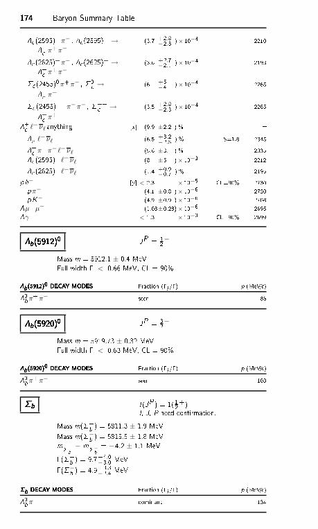
174174174174 Baryon Summary Table (2595)+π− , (2595)+ →+ π+π−
(3.7 +2.8−2.3 ) × 10−4 2210 (2625)+π− , (2625)+ →+ π+π−
(3.6 +2.7−2.1 ) × 10−4 2193 (2455)0π+π− , 0 →+ π−
(6 +5−4 ) × 10−4 2265 (2455)++π−π− , ++ →+ π+ (3.5 +2.8−2.3 ) × 10−4 2265+ ℓ−νℓ anything [x (9.9 ±2.2 ) % + ℓ−νℓ (6.5 +3.2−2.5 ) % S=1.8 2345+ π+π− ℓ−νℓ (5.6 ±3.1 ) % 2335 (2595)+ ℓ−νℓ (8 ±5 )× 10−3 2212 (2625)+ ℓ−νℓ (1.4 +0.9−0.7 ) % 2195ph− [y < 2.3 × 10⁻⁵ CL=90% 2730pπ− (4.1 ±0.8 )× 10−6 2730pK− (4.9 ±0.9 )× 10−6 2708µ+µ− (1.08±0.28)× 10−6 2695γ < 1.3 × 10⁻³ CL=90% 2699b(5912)0b(5912)0b(5912)0b(5912)0 JP = 12−Mass m = 5912.1 ± 0.4 MeVFull width < 0.66 MeV, CL = 90%b(5912)0 DECAY MODESb(5912)0 DECAY MODESb(5912)0 DECAY MODESb(5912)0 DECAY MODES Fra tion (i /) p (MeV/ )0b π+π− seen 86b(5920)0b(5920)0b(5920)0b(5920)0 JP = 32−Mass m = 5919.73 ± 0.32 MeVFull width < 0.63 MeV, CL = 90%b(5920)0 DECAY MODESb(5920)0 DECAY MODESb(5920)0 DECAY MODESb(5920)0 DECAY MODES Fra tion (i /) p (MeV/ )0b π+π− seen 108bbbb I (JP ) = 1(12+)I, J, P need onrmation.Mass m(+b ) = 5811.3 ± 1.9 MeVMass m(−b ) = 5815.5 ± 1.8 MeVm+b − m−b = −4.2 ± 1.1 MeV(+b ) = 9.7+4.0
−3.0 MeV(−b ) = 4.9+3.3−2.4 MeVb DECAY MODESb DECAY MODESb DECAY MODESb DECAY MODES Fra tion (i /) p (MeV/ )0b π dominant 134
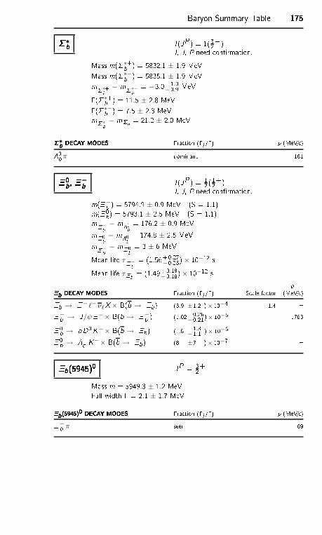
Baryon Summary Table 175175175175 ∗b ∗b ∗b ∗b I (JP ) = 1(32+)I, J, P need onrmation.Mass m(∗+b ) = 5832.1 ± 1.9 MeVMass m(∗−b ) = 5835.1 ± 1.9 MeVm∗+b − m∗−b = −3.0+1.0−0.9 MeV(∗+b ) = 11.5 ± 2.8 MeV(∗−b ) = 7.5 ± 2.3 MeVm∗b − mb = 21.2 ± 2.0 MeV∗b DECAY MODES∗b DECAY MODES∗b DECAY MODES∗b DECAY MODES Fra tion (i /) p (MeV/ )0b π dominant 161 0b, −b 0b, −b 0b, −b 0b, −b I (JP ) = 12 (12+)I, J, P need onrmation.m(−b ) = 5794.9 ± 0.9 MeV (S = 1.1)m( 0b) = 5793.1 ± 2.5 MeV (S = 1.1)m−b − m0b = 176.2 ± 0.9 MeVm0b − m0b = 174.8 ± 2.5 MeVm−b − m0b = 3 ± 6 MeVMean life τ−b = (1.56+0.27−0.25)× 10−12 sMean life τb = (1.49+0.19−0.18)× 10−12 s pb DECAY MODESb DECAY MODESb DECAY MODESb DECAY MODES Fra tion (i /) S ale fa tor (MeV/ )b → − ℓ−νℓX × B(b → b) (3.9 ±1.2 )× 10−4 1.4 −b → J/ψ−× B(b → −b ) (1.02+0.26
−0.21)× 10−5 1783 0b → pD0K−× B(b → b) (1.8 +1.3−1.1 )× 10−6 0b → + K−× B(b → b) (8 ±7 )× 10−7 b(5945)0b(5945)0b(5945)0b(5945)0 JP = 32+Mass m = 5949.3 ± 1.2 MeVFull width = 2.1 ± 1.7 MeVb(5945)0 DECAY MODESb(5945)0 DECAY MODESb(5945)0 DECAY MODESb(5945)0 DECAY MODES Fra tion (i /) p (MeV/ )−b π+ seen 69
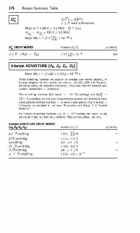
176176176176 Baryon Summary Table−b−b−b−b I (JP ) = 0(12+)I, J, P need onrmation.Mass m = 6048.8 ± 3.2 MeV (S = 1.5)m−b − m0b = 426.4 ± 2.2 MeVMean life τ = (1.1+0.5−0.4)× 10−12 s−b DECAY MODES−b DECAY MODES−b DECAY MODES−b DECAY MODES Fra tion (i /) p (MeV/ )J/ψ−×B(b → b) (2.9+1.1
−0.8)× 10−6 1808b-baryon ADMIXTURE (b, b, b, b)b-baryon ADMIXTURE (b, b, b, b)b-baryon ADMIXTURE (b, b, b, b)b-baryon ADMIXTURE (b, b, b, b)Mean life τ = (1.449 ± 0.015)× 10−12 sThese bran hing fra tions are a tually an average over weakly de aying b-baryons weighted by their produ tion rates at the LHC, LEP, and Tevatron,bran hing ratios, and dete tion eÆ ien ies. They s ale with the b-baryon pro-du tion fra tion B(b → b -baryon).The bran hing fra tions B(b -baryon → ℓ− νℓ anything) and B(0b →+ ℓ− νℓ anything) are not pure measurements be ause the underlying mea-sured produ ts of these with B(b → b -baryon) were used to determine B(b →b -baryon), as des ribed in the note \Produ tion and De ay of b-FlavoredHadrons."For in lusive bran hing fra tions, e.g., B → D± anything, the values usuallyare multipli ities, not bran hing fra tions. They an be greater than one.b-baryon ADMIXTURE DECAY MODESb-baryon ADMIXTURE DECAY MODESb-baryon ADMIXTURE DECAY MODESb-baryon ADMIXTURE DECAY MODES(b ,b ,b ,b)(b ,b ,b ,b)(b ,b,b ,b)(b ,b,b ,b) Fra tion (i /) p (MeV/ )pµ−ν anything ( 5.3+ 2.2− 1.9) % p ℓνℓ anything ( 5.1± 1.2) % p anything (64 ±21 ) % ℓ−νℓ anything ( 3.5± 0.6) % /anything (36 ± 7 ) % − ℓ−νℓ anything ( 6.0± 1.6)× 10−3
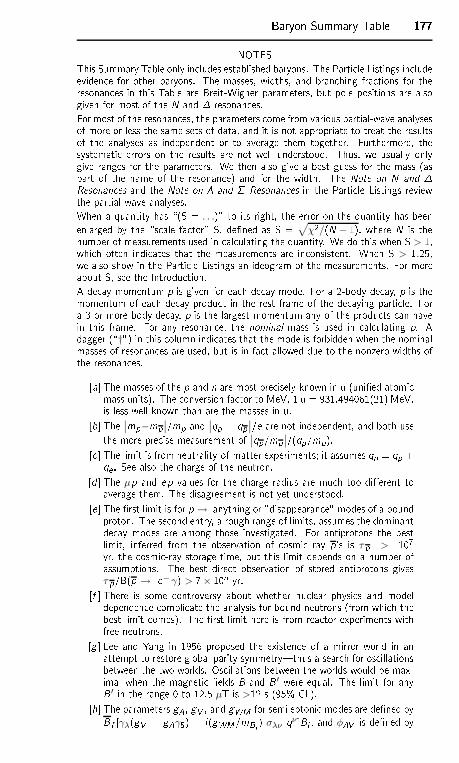
Baryon Summary Table 177177177177NOTESThis Summary Table only in ludes established baryons. The Parti le Listings in ludeeviden e for other baryons. The masses, widths, and bran hing fra tions for theresonan es in this Table are Breit-Wigner parameters, but pole positions are alsogiven for most of the N and resonan es.For most of the resonan es, the parameters ome from various partial-wave analysesof more or less the same sets of data, and it is not appropriate to treat the resultsof the analyses as independent or to average them together. Furthermore, thesystemati errors on the results are not well understood. Thus, we usually onlygive ranges for the parameters. We then also give a best guess for the mass (aspart of the name of the resonan e) and for the width. The Note on N and Resonan es and the Note on and Resonan es in the Parti le Listings reviewthe partial-wave analyses.When a quantity has \(S = . . .)" to its right, the error on the quantity has beenenlarged by the \s ale fa tor" S, dened as S = √
χ2/(N − 1), where N is thenumber of measurements used in al ulating the quantity. We do this when S > 1,whi h often indi ates that the measurements are in onsistent. When S > 1.25,we also show in the Parti le Listings an ideogram of the measurements. For moreabout S, see the Introdu tion.A de ay momentum p is given for ea h de ay mode. For a 2-body de ay, p is themomentum of ea h de ay produ t in the rest frame of the de aying parti le. Fora 3-or-more-body de ay, p is the largest momentum any of the produ ts an havein this frame. For any resonan e, the nominal mass is used in al ulating p. Adagger (\†") in this olumn indi ates that the mode is forbidden when the nominalmasses of resonan es are used, but is in fa t allowed due to the nonzero widths ofthe resonan es.[a The masses of the p and n are most pre isely known in u (unied atomi mass units). The onversion fa tor to MeV, 1 u = 931.494061(21) MeV,is less well known than are the masses in u.[b The ∣
∣mp−mp∣∣/mp and ∣
∣qp + qp∣∣/e are not independent, and both usethe more pre ise measurement of ∣
∣qp/mp∣∣/(qp/mp).[ The limit is from neutrality-of-matter experiments; it assumes qn = qp +qe . See also the harge of the neutron.[d The µp and e p values for the harge radius are mu h too dierent toaverage them. The disagreement is not yet understood.[e The rst limit is for p → anything or "disappearan e" modes of a boundproton. The se ond entry, a rough range of limits, assumes the dominantde ay modes are among those investigated. For antiprotons the bestlimit, inferred from the observation of osmi ray p's is τ p > 107yr, the osmi -ray storage time, but this limit depends on a number ofassumptions. The best dire t observation of stored antiprotons givesτ p/B(p → e−γ) > 7× 10⁵ yr.[f There is some ontroversy about whether nu lear physi s and modeldependen e ompli ate the analysis for bound neutrons (from whi h thebest limit omes). The rst limit here is from rea tor experiments withfree neutrons.[g Lee and Yang in 1956 proposed the existen e of a mirror world in anattempt to restore global parity symmetry|thus a sear h for os illationsbetween the two worlds. Os illations between the worlds would be max-imal when the magneti elds B and B ′ were equal. The limit for anyB ′ in the range 0 to 12.5 µT is >12 s (95% CL).[h The parameters gA, gV , and gWM for semileptoni modes are dened byB f [γλ(gV + gAγ5) + i(gWM/mBi ) σλν qν Bi , and φAV is dened by
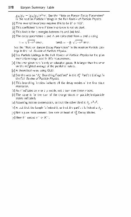
178178178178 Baryon Summary TablegA/gV = ∣
∣gA/gV ∣
∣eiφAV . See the \Note on Baryon De ay Parameters"in the neutron Parti le Listings in the Full Review of Parti le Physi s.[i Time-reversal invarian e requires this to be 0 or 180.[j This oeÆ ient is zero if time invarian e is not violated.[k This limit is for γ energies between 15 and 340 keV.[l The de ay parameters γ and are al ulated from α and φ usingγ = √1−α2 osφ , tan = −
1α
√1−α2 sinφ .See the \Note on Baryon De ay Parameters" in the neutron Parti le List-ings in the Full Review of Parti le Physi s.[n See Parti le Listings in the Full Review of Parti le Physi s for the pionmomentum range used in this measurement.[o The error given here is only an edu ated guess. It is larger than the erroron the weighted average of the published values.[p A theoreti al value using QED.[q See the note on \+ Bran hing Fra tions" in the + Parti le Listings inthe Full Review of Parti le Physi s.[r This bran hing fra tion in ludes all the de ay modes of the nal-stateresonan e.[s An ℓ indi ates an e or a µ mode, not a sum over these modes.[t The value is for the sum of the harge states or parti le/antiparti lestates indi ated.[u Assuming isospin onservation, so that the other third is + π0π0.[v A test that the isospin is indeed 0, so that the parti le is indeed a + .[x Not a pure measurement. See note at head of 0b De ay Modes.[y Here h− means π− or K−.
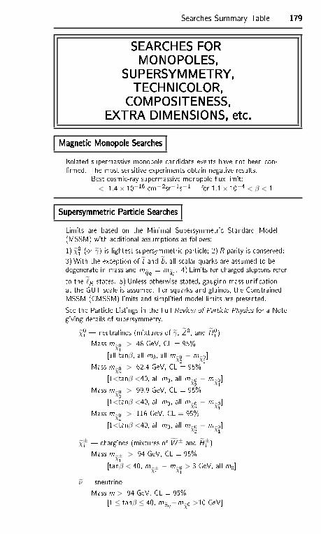
Sear hes Summary Table 179179179179SEARCHES FORSEARCHES FORSEARCHES FORSEARCHES FORMONOPOLES,MONOPOLES,MONOPOLES,MONOPOLES,SUPERSYMMETRY,SUPERSYMMETRY,SUPERSYMMETRY,SUPERSYMMETRY,TECHNICOLOR,TECHNICOLOR,TECHNICOLOR,TECHNICOLOR,COMPOSITENESS,COMPOSITENESS,COMPOSITENESS,COMPOSITENESS,EXTRA DIMENSIONS, et .EXTRA DIMENSIONS, et .EXTRA DIMENSIONS, et .EXTRA DIMENSIONS, et .Magneti Monopole Sear hesMagneti Monopole Sear hesMagneti Monopole Sear hesMagneti Monopole Sear hesIsolated supermassive monopole andidate events have not been on-rmed. The most sensitive experiments obtain negative results.Best osmi -ray supermassive monopole ux limit:< 1.4× 10⁻¹⁶ m−2sr−1s−1 for 1.1× 10⁻⁴ < β < 1Supersymmetri Parti le Sear hesSupersymmetri Parti le Sear hesSupersymmetri Parti le Sear hesSupersymmetri Parti le Sear hesLimits are based on the Minimal Supersymmetri Standard Model(MSSM) with additional assumptions as follows:1) χ01 (or γ) is lightest supersymmetri parti le; 2) R-parity is onserved;3) With the ex eption of t and b, all s alar quarks are assumed to bedegenerate in mass and mqR = mqL . 4) Limits for harged sleptons referto the ℓR states. 5) Unless otherwise stated, gaugino mass uni ationat the GUT s ale is assumed. For squarks and gluinos, the ConstrainedMSSM (CMSSM) limits and simplied model limits are presented.See the Parti le Listings in the Full Review of Parti le Physi s for a Notegiving details of supersymmetry.
χ0i | neutralinos (mixtures of γ, Z0, and H0i )Mass mχ01 > 46 GeV, CL = 95%[all tanβ, all m0, all mχ02 − m
χ01 Mass mχ02 > 62.4 GeV, CL = 95%[1<tanβ <40, all m0, all mχ02 − m
χ01 Mass mχ03 > 99.9 GeV, CL = 95%[1<tanβ <40, all m0, all mχ02 − m
χ01 Mass mχ04 > 116 GeV, CL = 95%[1<tanβ <40, all m0, all mχ02 − m
χ01 χ±i | harginos (mixtures of W± and H±i )Mass m
χ±1 > 94 GeV, CL = 95%[tanβ < 40, mχ±1 − m
χ01 > 3 GeV, all m0ν | sneutrinoMass m > 94 GeV, CL = 95%[1 ≤ tanβ ≤ 40, m eR−m
χ01 >10 GeV
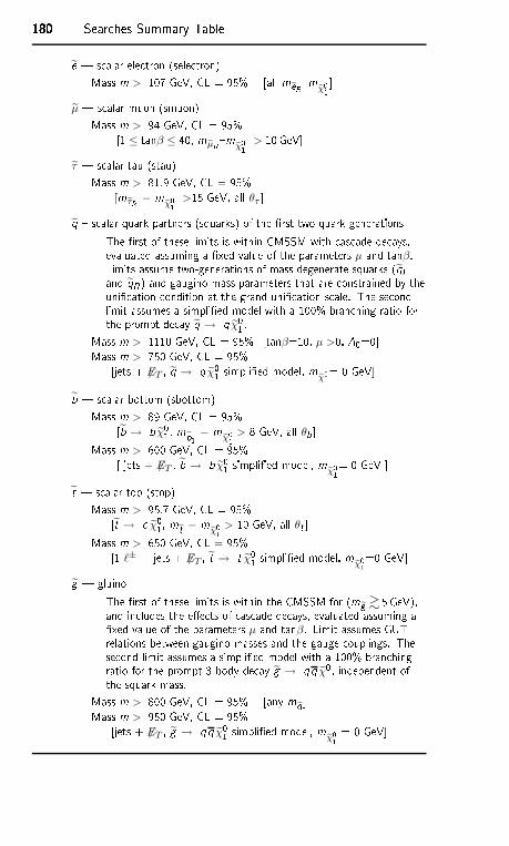
180180180180 Sear hes Summary Tablee | s alar ele tron (sele tron)Mass m > 107 GeV, CL = 95% [all meRmχ01 µ | s alar muon (smuon)Mass m > 94 GeV, CL = 95%[1 ≤ tanβ ≤ 40, mµR mχ01 > 10 GeVτ | s alar tau (stau)Mass m > 81.9 GeV, CL = 95%[mτR − m
χ01 >15 GeV, all θτ q s alar quark partners (squarks) of the rst two quark generationsThe rst of these limits is within CMSSM with as ade de ays,evaluated assuming a xed value of the parameters µ and tanβ.Limits assume two-generations of mass degenerate squarks (qLand qR) and gaugino mass parameters that are onstrained by theuni ation ondition at the grand uni ation s ale. The se ondlimit assumes a simplied model with a 100% bran hing ratio forthe prompt de ay q → q χ01.Mass m > 1110 GeV, CL = 95% [tanβ=10, µ >0, A0=0Mass m > 750 GeV, CL = 95%[jets + 6ET , q → q χ01 simplied model, mχ01= 0 GeVb | s alar bottom (sbottom)Mass m > 89 GeV, CL = 95%[b → b χ01, mb1 − m
χ01 > 8 GeV, all θbMass m > 600 GeV, CL = 95%[ jets + 6ET , b → b χ01 simplied model, mχ01= 0 GeV t | s alar top (stop)Mass m > 95.7 GeV, CL = 95%[t → χ01, m t − m
χ01 > 10 GeV, all θt Mass m > 650 GeV, CL = 95%[1 ℓ± + jets + 6ET , t → t χ01 simplied model, mχ01=0 GeVg | gluinoThe rst of these limits is within the CMSSM for (mg & 5 GeV),and in ludes the ee ts of as ade de ays, evaluated assuming axed value of the parameters µ and tanβ. Limit assumes GUTrelations between gaugino masses and the gauge ouplings. These ond limit assumes a simplied model with a 100% bran hingratio for the prompt 3 body de ay g → qq χ01, independent ofthe squark mass.Mass m > 800 GeV, CL = 95% [any mq Mass m > 950 GeV, CL = 95%[jets + 6ET , g → qq χ01 simplied model, m
χ01 = 0 GeV
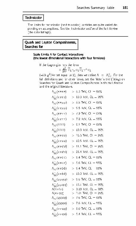
Sear hes Summary Table 181181181181Te hni olorTe hni olorTe hni olorTe hni olorThe limits for te hni olor (and top- olor) parti les are quite varied de-pending on assumptions. See the Te hni olor se tion of the full Review(the data listings).Quark and Lepton Compositeness,Quark and Lepton Compositeness,Quark and Lepton Compositeness,Quark and Lepton Compositeness,Sear hes forSear hes forSear hes forSear hes forS ale Limits for Conta t Intera tionsS ale Limits for Conta t Intera tionsS ale Limits for Conta t Intera tionsS ale Limits for Conta t Intera tions(the lowest dimensional intera tions with four fermions)(the lowest dimensional intera tions with four fermions)(the lowest dimensional intera tions with four fermions)(the lowest dimensional intera tions with four fermions)If the Lagrangian has the form±
g222 ψL γµ ψLψL γ µ ψL(with g2/4π set equal to 1), then we dene ≡ ±LL. For thefull denitions and for other forms, see the Note in the Listings onSear hes for Quark and Lepton Compositeness in the full Reviewand the original literature.+LL(e e e e) > 8.3 TeV, CL = 95%−LL(e e e e) > 10.3 TeV, CL = 95%+LL(e eµµ) > 8.5 TeV, CL = 95%−LL(e eµµ) > 9.5 TeV, CL = 95%+LL(e e τ τ) > 7.9 TeV, CL = 95%−LL(e e τ τ) > 7.2 TeV, CL = 95%+LL(ℓℓℓℓ) > 9.1 TeV, CL = 95%−LL(ℓℓℓℓ) > 10.3 TeV, CL = 95%+LL(e e uu) > 23.3 TeV, CL = 95%−LL(e e uu) > 12.5 TeV, CL = 95%+LL(e e d d) > 11.1 TeV, CL = 95%−LL(e e d d) > 26.4 TeV, CL = 95%+LL(e e ) > 9.4 TeV, CL = 95%−LL(e e ) > 5.6 TeV, CL = 95%+LL(e e bb) > 9.4 TeV, CL = 95%−LL(e e bb) > 10.2 TeV, CL = 95%+LL(µµqq) > 9.6 TeV, CL = 95%−LL(µµqq) > 13.1 TeV, CL = 95%(ℓν ℓν) > 3.10 TeV, CL = 90%(e ν qq) > 2.81 TeV, CL = 95%+LL(qqqq) > 7.6 TeV, CL = 95%−LL(qqqq) > 7.6 TeV, CL = 95%+LL(ν ν qq) > 5.0 TeV, CL = 95%−LL(ν ν qq) > 5.4 TeV, CL = 95%
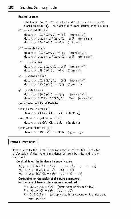
182182182182 Sear hes Summary TableEx ited LeptonsEx ited LeptonsEx ited LeptonsEx ited LeptonsThe limits from ℓ∗+ ℓ∗− do not depend on λ (where λ is the ℓℓ∗transition oupling). The λ-dependent limits assume hiral oupling.e∗± | ex ited ele tronMass m > 103.2 GeV, CL = 95% (from e∗ e∗)Mass m > 2.200× 10³ GeV, CL = 95% (from e e∗)Mass m > 356 GeV, CL = 95% (if λγ = 1)µ∗± | ex ited muonMass m > 103.2 GeV, CL = 95% (from µ∗µ∗)Mass m > 2.200× 10³ GeV, CL = 95% (from µµ∗)τ∗± | ex ited tauMass m > 103.2 GeV, CL = 95% (from τ∗ τ∗)Mass m > 185 GeV, CL = 95% (from τ τ∗)ν∗ | ex ited neutrinoMass m > 102.6 GeV, CL = 95% (from ν∗ ν∗)Mass m > 213 GeV, CL = 95% (from ν ν∗)q∗ | ex ited quarkMass m > 338 GeV, CL = 95% (from q∗q∗)Mass m > 3.500× 10³ GeV, CL = 95% (from q∗X)Color Sextet and O tet Parti lesColor Sextet and O tet Parti lesColor Sextet and O tet Parti lesColor Sextet and O tet Parti lesColor Sextet Quarks (q6)Mass m > 84 GeV, CL = 95% (Stable q6)Color O tet Charged Leptons (ℓ8)Mass m > 86 GeV, CL = 95% (Stable ℓ8)Color O tet Neutrinos (ν8)Mass m > 110 GeV, CL = 90% (ν8 → ν g )Extra DimensionsExtra DimensionsExtra DimensionsExtra DimensionsPlease refer to the Extra Dimensions se tion of the full Review fora dis ussion of the model-dependen e of these bounds, and further onstraints.Constraints on the fundamental gravity s aleConstraints on the fundamental gravity s aleConstraints on the fundamental gravity s aleConstraints on the fundamental gravity s aleMTT > 3.2 TeV, CL = 95% (pp → e+ e−, µ+µ−, γ γ)MC > 4.16 TeV, CL = 95% (pp → ℓℓ)MD > 2.16 TeV, CL = 95% (pp → G → ℓℓ)Constraints on the radius of the extra dimensions,Constraints on the radius of the extra dimensions,Constraints on the radius of the extra dimensions,Constraints on the radius of the extra dimensions,for the ase of two- at dimensions of equal radiifor the ase of two- at dimensions of equal radiifor the ase of two- at dimensions of equal radiifor the ase of two- at dimensions of equal radiiR < 30 µm, CL = 95% (dire t tests of Newton's law)R < 23 µm, CL = 95% (pp → j G )R < 0.16916 nm (astrophysi s; limits depend on te hnique andassumptions)
Tests of Conservation Laws 183183183183TESTS OF CONSERVATION LAWS
Updated May 2014 by L. Wolfenstein (Carnegie-Mellon University)and C.-J. Lin (LBNL).
In keeping with the current interest in tests of conservation laws,
we collect together a Table of experimental limits on all weak and
electromagnetic decays, mass differences, and moments, and on a
few reactions, whose observation would violate conservation laws.
The Table is given only in the full Review of Particle Physics, not in
the Particle Physics Booklet. For the benefit of Booklet readers, we
include the best limits from the Table in the following text. Limits
in this text are for CL=90% unless otherwise specified. The Table is
in two parts: “Discrete Space-Time Symmetries,” i.e., C, P , T , CP ,
and CPT ; and “Number Conservation Laws,” i.e., lepton, baryon,
hadronic flavor, and charge conservation. The references for these
data can be found in the the Particle Listings in the Review. A
discussion of these tests follows.
CPT INVARIANCE
General principles of relativistic field theory require invariance un-
der the combined transformation CPT . The simplest tests of CPT
invariance are the equality of the masses and lifetimes of a particle
and its antiparticle. The best test comes from the limit on the mass
difference between K0 and K0. Any such difference contributes to
the CP -violating parameter ǫ. Assuming CPT invariance, φǫ, the
phase of ǫ should be very close to 44. (See the review “CP Viola-
tion in KL decay” in this edition.) In contrast, if the entire source
of CP violation in K0 decays were a K0 − K0
mass difference, φǫ
would be 44 + 90.
Assuming that there is no other source of CPT violation than this
mass difference, it is possible to deduce that[1]
mK
0 − mK0 ≈2(mK0
L
− mK0
S
) |η| ( 2
3φ+− + 1
3φ00 − φSW)
sin φSW
,
where φSW = (43.51 ± 0.05), the superweak angle. Using our
best values of the CP -violation parameters, we get |(mK
0 −
mK0)/mK0 | ≤ 0.6 × 10⁻¹⁸ at CL=90%. Limits can also be placed
on specific CPT -violating decay amplitudes. Given the small value
of (1 − |η00/η+−|), the value of φ00 − φ+− provides a measure of
184184184184 Tests of Conservation LawsCPT violation in K0
L → 2π decay. Results from CERN [1] and
Fermilab [2] indicate no CPT -violating effect.
CP AND T INVARIANCE
Given CPT invariance, CP violation and T violation are equiv-
alent. The original evidence for CP violation came from the
measurement of |η+−| = |A(K0L → π+π−)/A(K0
S → π+π−)| =
(2.232± 0.011)× 10−3. This could be explained in terms of K0–K0
mixing, which also leads to the asymmetry [Γ(K0L → π−e+ν) −
Γ(K0L → π+e−ν)]/[sum] = (0.334± 0.007)%. Evidence for CP vio-
lation in the kaon decay amplitude comes from the measurement of
(1 − |η00/η+−|)/3 = Re(ǫ′/ǫ) = (1.66 ± 0.23) × 10−3. In the Stan-
dard Model much larger CP -violating effects are expected. The
first of these, which is associated with B–B mixing, is the param-
eter sin(2β) now measured quite accurately to be 0.682 ± 0.019.
A number of other CP -violating observables are being measured
in B decays; direct evidence for CP violation in the B decay am-
plitude comes from the asymmetry [Γ(B0→ K−π+) − Γ(B0 →
K+π−)]/[sum] = −0.082 ± 0.006. Direct tests of T violation are
much more difficult; a measurement by CPLEAR of the difference
between the oscillation probabilities of K0 to K0 and K0 to K0 is
related to T violation [3]. A nonzero value of the electric dipole
moment of the neutron and electron requires both P and T viola-
tion. The current experimental results are < 2.9×10⁻²⁶ e cm (neu-
tron), and < (10.5 ± 0.07) × 10−28 e cm (electron). The BABAR
experiment has reported the first direct observation of T violation
in the B system. The measured T -violating parameters in the time
evolution of the neutral B mesons are ∆S+T = −1.37 ± 0.15 and
∆S−
T = 1.17± 0.21, with a significance of 14σ [4]. This observation
of T violation, with exchange of initial and final states of the neutral
B, was made possible in a B-factory using the Einstein-Podolsky-
Rosen Entanglement of the two B’s produced in the decay of the
Υ(4S) and the two time-ordered decays of the B’s as filtering mea-
surements of the meson state [5].
CONSERVATION OF LEPTON NUMBERS
Present experimental evidence and the standard electroweak theory
are consistent with the absolute conservation of three separate lep-
ton numbers: electron number Le, muon number Lµ, and tau num-
ber Lτ , except for the effect of neutrino mixing associated with
neutrino masses. Searches for violations are of the following types:
Tests of Conservation Laws 185185185185a) ∆L = 2 for one type of charged lepton. The best limit
comes from the search for neutrinoless double beta decay (Z, A)
→ (Z + 2, A)+e−+e−. The best laboratory limit is t1/2 > 2.1×1025
yr (CL=90%) for 76Ge.
b) Conversion of one charged-lepton type to another. For
purely leptonic processes, the best limits are on µ → eγ and
µ → 3e, measured as Γ(µ → eγ)/Γ(µ →all) < 5.7 × 10⁻¹³ and
Γ(µ → 3e)/Γ(µ → all) < 1.0 × 10⁻¹². For semileptonic pro-
cesses, the best limit comes from the coherent conversion pro-
cess in a muonic atom, µ−+ (Z, A) → e− + (Z, A), measured as
Γ(µ−Ti → e−Ti)/Γ(µ−Ti → all) < 4.3 × 10⁻¹². Of special interest
is the case in which the hadronic flavor also changes, as in KL → eµ
and K+ → π+e−µ+, measured as Γ(KL → eµ)/Γ(KL → all) <
4.7 × 10⁻¹² and Γ(K+ → π+e−µ+)/Γ(K+ → all) < 1.3 × 10⁻¹¹.
Limits on the conversion of τ into e or µ are found in τ decay
and are much less stringent than those for µ → e conversion, e.g.,
Γ(τ → µγ)/Γ(τ → all) < 4.4 × 10⁻⁸ and Γ(τ → eγ)/Γ(τ → all) <
3.3 × 10⁻⁸.
c) Conversion of one type of charged lepton into an-
other type of charged antilepton. The case most studied is
µ−+(Z, A) → e+ + (Z − 2, A), the strongest limit being Γ(µ−Ti →
e+Ca)/Γ(µ−Ti → all) < 3.6 × 10⁻¹¹.
d) Neutrino oscillations. It is expected even in the standard
electroweak theory that the lepton numbers are not separately con-
served, as a consequence of lepton mixing analogous to Cabibbo-
Kobayashi-Maskawa quark mixing. However, if the only source
of lepton-number violation is the mixing of low-mass neutrinos
then processes such as µ → eγ are expected to have extremely
small unobservable probabilities. For small neutrino masses, the
lepton-number violation would be observed first in neutrino os-
cillations, which have been the subject of extensive experimental
studies. Compelling evidence for neutrino mixing has come from
atmospheric, solar, accelerator, and reactor neutrinos. Recently,
the reactor neutrino experiments have measured the last neutrino
mixing angle θ13 and found it to be relatively large. For a compre-
hensive review on neutrino mixing, including the latest results on
θ13, see the review “Neutrino Mass, Mixing, and Oscillations” by
K. Nakamura and S.T. Petcov in this edition of RPP.
186186186186 Tests of Conservation LawsCONSERVATION OF HADRONIC FLAVORS
In strong and electromagnetic interactions, hadronic flavor
is conserved, i.e. the conversion of a quark of one flavor
(d, u, s, c, b, t) into a quark of another flavor is forbidden. In the
Standard Model, the weak interactions violate these conservation
laws in a manner described by the Cabibbo-Kobayashi-Maskawa
mixing (see the section “Cabibbo-Kobayashi-Maskawa Mixing Ma-
trix”). The way in which these conservation laws are violated is
tested as follows:
(a) ∆S = ∆Q rule. In the strangeness-changing semileptonic decay
of strange particles, the strangeness change equals the change in
charge of the hadrons. Tests come from limits on decay rates such
as Γ(Σ+ → ne+ν)/Γ(Σ+ → all) < 5 × 10⁻⁶, and from a detailed
analysis of KL → πeν, which yields the parameter x, measured to
be (Re x, Im x) = (−0.002±0.006, 0.0012±0.0021). Corresponding
rules are ∆C = ∆Q and ∆B = ∆Q.
(b) Change of flavor by two units. In the Standard Model this
occurs only in second-order weak interactions. The classic example
is ∆S = 2 via K0 − K0
mixing, which is directly measured by
m(KL) − m(KS) = (0.5293 ± 0.0009) × 1010 hs−1. The ∆B =
2 transitions in the B0 and B0s systems via mixing are also well
established. The measured mass differences between the eigenstates
are (mB0
H
− mB0
L
) = (0.510±0.003)×1012 hs−1 and (mB0
sH
− mB0
sL
)
= (17.761 ± 0.022) × 1012 hs−1. There is now strong evidence of
∆C = 2 transition in the charm sector with the mass difference
mD0
H
− mD0
L
= (0.95+0.41−0.44) × 1010 hs−1. All results are consistent
with the second-order calculations in the Standard Model.
(c) Flavor-changing neutral currents. In the Standard Model
the neutral-current interactions do not change flavor. The low
rate Γ(KL → µ+µ−)/Γ(KL → all) = (6.84 ± 0.11) × 10−9 puts
limits on such interactions; the nonzero value for this rate is at-
tributed to a combination of the weak and electromagnetic in-
teractions. The best test should come from K+ → π+νν,
which occurs in the Standard Model only as a second-order weak
process with a branching fraction of (0.4 to 1.2)×10−10. Com-
bining results from BNL-E787 and BNL-E949 experiments yield
Tests of Conservation Laws 187187187187Γ(K+ → π+νν)/Γ(K+ → all) = (1.7 ± 1.1) × 10−10[6]. Lim-
its for charm-changing or bottom-changing neutral currents are
less stringent: Γ(D0 → µ+µ−)/Γ(D0 → all) < 6.2 × 10⁻⁹ and
Γ(B0 → µ+µ−)/Γ(B0 → all) < 6.3 × 10⁻¹⁰. One cannot isolate
flavor-changing neutral current (FCNC) effects in non leptonic de-
cays. For example, the FCNC transition s → d+(u+u) is equivalent
to the charged-current transition s → u + (u + d). Tests for FCNC
are therefore limited to hadron decays into lepton pairs. Such de-
cays are expected only in second-order in the electroweak coupling
in the Standard Model. The LHCb and CMS experiments have re-
cently observed the FCNC decay of B0s → µ+µ−. The current world
average value is Γ(B0s → µ+µ−)/Γ(B0
s → all) = (3.1± 0.7)× 10−9,
which is consistent with the Standard Model expectation.
See the full Review of Particle Physics for references and Summary Tables.
188 9. Quantum chromodynamics
9. QUANTUM CHROMODYNAMICS
Revised October 2013 by S. Bethke (Max-Planck-Institute of Physics,Munich), G. Dissertori (ETH Zurich), and G.P. Salam (CERN andLPTHE, Paris).
9.1. Basics
Quantum Chromodynamics (QCD), the gauge field theory thatdescribes the strong interactions of colored quarks and gluons, is the SU(3)component of the SU(3)×SU(2)×U(1) Standard Model of Particle Physics.
The Lagrangian of QCD is given by
L =∑
q
ψq,a(iγµ∂µδab − gsγµtCabA
Cµ − mqδab)ψq,b −
1
4FA
µνFA µν , (9.1)
where repeated indices are summed over. The γµ are the Dirac γ-matrices.The ψq,a are quark-field spinors for a quark of flavor q and mass mq, witha color-index a that runs from a = 1 to Nc = 3, i.e. quarks come in three“colors.” Quarks are said to be in the fundamental representation of theSU(3) color group.
The ACµ correspond to the gluon fields, with C running from 1 to
N2c − 1 = 8, i.e. there are eight kinds of gluon. Gluons transform under
the adjoint representation of the SU(3) color group. The tCab correspondto eight 3 × 3 matrices and are the generators of the SU(3) group (cf. thesection on “SU(3) isoscalar factors and representation matrices” in thisReview with tCab ≡ λC
ab/2). They encode the fact that a gluon’s interactionwith a quark rotates the quark’s color in SU(3) space. The quantity gs isthe QCD coupling constant. Finally, the field tensor FA
µν is given by
FAµν = ∂µA
Aν − ∂νA
Aµ − gs fABCA
Bµ A
Cν [tA, tB] = ifABCtC , (9.2)
where the fABC are the structure constants of the SU(3) group.
Neither quarks nor gluons are observed as free particles. Hadrons arecolor-singlet (i.e. color-neutral) combinations of quarks, anti-quarks, andgluons.
Ab-initio predictive methods for QCD include lattice gauge theoryand perturbative expansions in the coupling. The Feynman rules of QCDinvolve a quark-antiquark-gluon (qqg) vertex, a 3-gluon vertex (bothproportional to gs), and a 4-gluon vertex (proportional to g2
s). A full setof Feynman rules is to be found for example in Ref. 1.
Useful color-algebra relations include: tAabtAbc = CF δac, where CF ≡
(N2c −1)/(2Nc) = 4/3 is the color-factor (“Casimir”) associated with gluon
emission from a quark; fACDfBCD = CAδAB where CA ≡ Nc = 3 is thecolor-factor associated with gluon emission from a gluon; tAabt
Bab = TRδAB,
where TR = 1/2 is the color-factor for a gluon to split to a qq pair.
The fundamental parameters of QCD are the coupling gs (or αs =g2s
4π)
and the quark masses mq.
9.1.1. Running coupling : In the framework of perturbative QCD(pQCD), predictions for observables are expressed in terms of the renor-malized coupling αs(µ
2R), a function of an (unphysical) renormalization
scale µR. When one takes µR close to the scale of the momentum transferQ in a given process, then αs(µ
2R ≃ Q2) is indicative of the effective
strength of the strong interaction in that process.
9. Quantum chromodynamics 189
The coupling satisfies the following renormalization group equation(RGE):
µ2R
dαs
dµ2R
= β(αs) = −(b0α2s + b1α
3s + b2α
4s + · · ·) (9.3)
where b0 = (11CA − 4nfTR)/(12π) = (33 − 2nf )/(12π) is referredto as the 1-loop beta-function coefficient, the 2-loop coefficient isb1 = (17C2
A −nfTR(10CA +6CF ))/(24π2) = (153−19nf)/(24π2), and the
3-loop coefficient is, in MS scheme, b2 = (2857− 50339 nf + 325
27 n2f )/(128π3)
for the SU(3) values of CA and CF . The 4-loop coefficient, b3, is tobe found in Refs. 10, 11. The minus sign in Eq. (9.3) is the origin ofAsymptotic Freedom, i.e. the fact that the strong coupling becomes weakfor processes involving large momentum transfers (“hard processes”),αs ∼ 0.1 for momentum transfers in the 100 GeV – TeV range.
The β-function coefficients, the bi, are given for the coupling of aneffective theory in which nf of the quark flavors are considered light(mq ≪ µR), and in which the remaining heavier quark flavors decouplefrom the theory. One may relate the coupling for the theory with nf + 1light flavors to that with nf flavors through an equation of the form
α(nf+1)s (µ2
R) = α(nf )s (µ2
R)
(
1 +
∞∑
n=1
n∑
ℓ=0
cnℓ [α(nf )s (µ2
R)]n lnℓ µ2R
m2h
)
, (9.4)
where mh is the mass of the (nf +1)th flavor, and the first few cnℓ
coefficients are c11 = 16π , c10 = 0, c22 = c211, c21 = 19
24π2, and c20 = − 11
72π2
when mh is the MS mass at scale mh (c20 = 724π2
when mh is the polemass — mass definitions are discussed below and in the review on “QuarkMasses”). Terms up to c4ℓ are to be found in Refs. 12, 13. Numerically,when one chooses µR = mh, the matching is a modest effect, owing to thezero value for the c10 coefficient.
Working in an energy range where the number of flavors is takenconstant, a simple exact analytic solution exists for Eq. (9.3) only if oneneglects all but the b0 term, giving αs(µ
2R) = (b0 ln(µ2
R/Λ2))−1. HereΛ is a constant of integration, which corresponds to the scale wherethe perturbatively-defined coupling would diverge, i.e. it is the non-perturbative scale of QCD. A convenient approximate analytic solution tothe RGE that includes also the b1, b2, and b3 terms is given by (see forexample Ref. 15),
αs(µ2R) ≃
1
b0t
(
1 −b1
b20
ln t
t+
b21(ln2 t − ln t − 1) + b0b2
b40t2
(9.5)
−
b31(ln3 t −
5
2ln2 t − 2 ln t +
1
2) + 3b0b1b2 ln t −
1
2b20b3
b60t3
, t ≡ ln
µ2R
Λ2,
again parametrized in terms of a constant Λ. Note that Eq. (9.5) is one ofseveral possible approximate 4-loop solutions for αs(µ
2R), and that a value
for Λ only defines αs(µ2R) once one knows which particular approximation
is being used. An alternative to the use of formulas such as Eq. (9.5)is to solve the RGE exactly, numerically (including the discontinuities,Eq. (9.4), at flavor thresholds). In such cases the quantity Λ is not defined
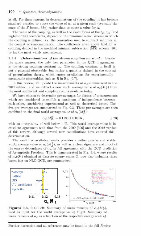
190 9. Quantum chromodynamics
at all. For these reasons, in determinations of the coupling, it has becomestandard practice to quote the value of αs at a given scale (typically themass of the Z boson, MZ) rather than to quote a value for Λ.
The value of the coupling, as well as the exact forms of the b2, c10 (andhigher-order) coefficients, depend on the renormalization scheme in whichthe coupling is defined, i.e. the convention used to subtract infinities inthe context of renormalization. The coefficients given above hold for acoupling defined in the modified minimal subtraction (MS) scheme [16],by far the most widely used scheme.
9.3.4. Determinations of the strong coupling constant : Besidethe quark masses, the only free parameter in the QCD Lagrangianis the strong coupling constant αs. The coupling constant in itself isnot a physical observable, but rather a quantity defined in the contextof perturbation theory, which enters predictions for experimentallymeasurable observables, such as R in Eq. (9.7).
In this review, we update the measurements of αs summarized in the2012 edition, and we extract a new world average value of αs(M
2Z) from
the most significant and complete results available today.
We have chosen to determine pre-averages for classes of measurementswhich are considered to exhibit a maximum of independence betweeneach other, considering experimental as well as theoretical issues. Thefive pre-averages are summarized in Fig. 9.3. These pre-averages are thencombined to the final world average value of αs(M
2Z):
αs(M2Z) = 0.1185± 0.0006 , (9.23)
with an uncertainty of well below 1 %. This world average value is inexcellent agreement with that from the 2009 [306] and the 2012 versionof this review, although several new contributions have entered thisdetermination.
The wealth of available results provides a rather precise and stableworld average value of αs(M
2Z), as well as a clear signature and proof of
the energy dependence of αs, in full agreement with the QCD predictionof Asymptotic Freedom. This is demonstrated in Fig. 9.4, where resultsof αs(Q
2) obtained at discrete energy scales Q, now also including thosebased just on NLO QCD, are summarized.
0.11 0.12 0.13α (Μ )s Ζ
LatticeDIS e+e- annihilation
τ-decays
Z pole fits
QCD αs(Mz) = 0.1185 ± 0.0006
Z pole fit
0.1
0.2
0.3
αs (Q)
1 10 100Q [GeV]
Heavy Quarkonia (NLO)
e+e– jets & shapes (res. NNLO)
DIS jets (NLO)
Sept. 2013
Lattice QCD (NNLO)
(N3LO)
τ decays (N3LO)
1000
pp –> jets (NLO)(–)
Figures 9.3, 9.4: Left: Summary of measurements of αs(M2Z),
used as input for the world average value; Right: Summary ofmeasurements of αs as a function of the respective energy scale Q.
Further discussion and all references may be found in the full Review.
10. Electroweak model and constraints on new physics 191
10. ELECTROWEAK MODEL AND
CONSTRAINTS ON NEW PHYSICS
Revised Nov. 2013 by J. Erler (U. Mexico) and A. Freitas (Pittsburgh U.).
10.1. Introduction
The standard model of the electroweak interactions (SM) [1] isbased on the gauge group SU(2) × U(1), with gauge bosons W i
µ,i = 1, 2, 3, and Bµ for the SU(2) and U(1) factors, respectively,and the corresponding gauge coupling constants g and g′. The left-handed fermion fields of the ith fermion family transform as doublets
Ψi =
(νi
ℓ−i
)and
(ui
d′i
)under SU(2), where d′i ≡
∑j Vij dj , and V is
the Cabibbo-Kobayashi-Maskawa mixing matrix. [Constraints on V arediscussed in the Section on “The CKM Quark-Mixing Matrix”. Theextension of the mixing formalism to leptons is discussed in the Section on“Neutrino Mass, Mixing, and Oscillations”.] The right-handed fields areSU(2) singlets. In the minimal model there are three fermion families.
A complex scalar Higgs doublet, φ ≡(
φ+
φ0
), is added to the model for
mass generation through spontaneous symmetry breaking with potentialgiven by,
V (φ) = µ2φ†φ +λ2
2(φ†φ)2. (10.1)
For µ2 negative, φ develops a vacuum expectation value, v/√
2 = µ/λ,where v ≈ 246 GeV, breaking part of the electroweak (EW) gaugesymmetry, after which only one neutral Higgs scalar, H , remains in thephysical particle spectrum. In non-minimal models there are additionalcharged and neutral scalar Higgs particles [3].
After symmetry breaking the Lagrangian for the fermions, ψi, is
LF =∑
i
ψi
(i 6∂ − mi −
miH
v
)ψi
− g
2√
2
∑
i
Ψi γµ (1 − γ5)(T+ W+µ + T− W−
µ )Ψi (10.2)
− e∑
i
Qi ψi γµ ψi Aµ − g
2 cos θW
∑
i
ψi γµ(giV − gi
Aγ5)ψi Zµ .
Here θW ≡ tan−1(g′/g) is the weak angle; e = g sin θW is the positronelectric charge; and A ≡ B cos θW + W 3 sin θW is the photon field (γ).W± ≡ (W 1 ∓ iW 2)/
√2 and Z ≡ −B sin θW + W 3 cos θW are the charged
and neutral weak boson fields, respectively. The Yukawa coupling of H toψi in the first term in LF , which is flavor diagonal in the minimal model,is gmi/2MW . The boson masses in the EW sector are given (at tree level,i.e., to lowest order in perturbation theory) by,
MH = λ v, (10.3a)
MW =1
2g v =
e v
2 sin θW, (10.3b)
MZ =1
2
√g2 + g′2 v =
e v
2 sin θW cos θW=
MW
cos θW, (10.3c)
192 10. Electroweak model and constraints on new physics
Mγ = 0. (10.3d)
The second term in LF represents the charged-current weak interac-tion [4–7], where T+ and T− are the weak isospin raising and loweringoperators. For example, the coupling of a W to an electron and a neutrinois
− e
2√
2 sin θW
[W−
µ e γµ(1 − γ5)ν + W+µ ν γµ (1 − γ5)e
]. (10.4)
For momenta small compared to MW , this term gives rise to the effectivefour-fermion interaction with the Fermi constant given by GF /
√2 =
1/2v2 = g2/8M2W . The third term in LF describes electromagnetic
interactions (QED) [8–10], and the last is the weak neutral-currentinteraction [5–7]. Here
giV ≡ t3L(i) − 2Qi sin2 θW , gi
A ≡ t3L(i), (10.5)
where t3L(i) and Qi are the weak isospin and charge ψi, respectively.
The first term in Eq. (10.2) also gives rise to fermion masses, and inthe presence of right-handed neutrinos to Dirac neutrino masses. Thepossibility of Majorana masses is discussed in the Section on “NeutrinoMass, Mixing, and Oscillations”.
10.2. Renormalization and radiative corrections
In addition to the Higgs boson mass, MH , the fermion massesand mixings, and the strong coupling constant, αs, the SM has threeparameters. The set with the smallest experimental errors contains theZ mass, MZ = 91.1876 ± 0.0021 GeV, which has been determinedfrom the Z lineshape scan at LEP 1 [11], the Fermi constant,GF = 1.1663787(6) × 10−5 GeV−2, which is derived from the muonlifetime, and the fine structure constant, α = 1/137.035999074(44), whichis best determined from the e± anomalous magnetic moment [10]. It
is convenient to define a running α(Q) =α
1 − ∆α(Q)dependent on the
energy scale Q of the process. The hadronic contributions to ∆α, ∆α(5)had,
is non-perturbative for low Q and can be derived from e+e− annihilation
and τ decay data. Various evaluations of ∆α(5)had are summarized in
Table 10.1 in the full Review. For the top quark pole mass, we usemt = 173.24±0.81 GeV, which is an average of Tevatron [48] and LHC [49]data.
sin2 θW and MW can be calculated from from these inputs, orconversely, MH can be constrained by sin2 θW and MW . The valueof sin2 θW is extracted from neutral-current processes (see Sec. 10.3in the full Review) and Z pole observables (see Sec. 10.4 in the fullReview) and depends on the renormalization prescription. There are anumber of popular schemes [52–58] leading to values which differ bysmall factors depending on mt and MH , including the on-shell definitions2W ≡ 1 − M2
W /M2Z , the MS definition s 2
Z , and the effective angle
s2f = sin θf
eff .
Experiments are at such level of precision that complete one-loop,dominant two-loop, and partial three-loop radiative corrections must beapplied. These are discussed in the full edition of this Review. A varietyof related cross-section, asymmetry and decay formulae are also discussedthere.

10. Electroweak model and constraints on new physics 193
Figure 10.2: Scale dependence of the weak mixing angle in the MS
scheme [118]. The width of the curve reflects the theory uncertaintyfrom strong interaction effects which at low energies is at the levelof ±7 × 10⁻⁵ [118]. For NuTeV we display the updated valuefrom Ref. 120. for ν and ν interactions at NuTeV. The Tevatron andLHC measurements are strongly dominated by invariant masses ofthe final state dilepton pair of O(MZ) and can thus be considered asadditional Z pole data points. For clarity we displayed the Tevatronpoint horizontally to the left.
10.4.5. H decays :
The ATLAS and CMS collaborations at LHC observed a Higgsboson [180] with properties appearing well consistent with the SM Higgs(see the note on “The Higgs Boson H0 ” in the Gauge & Higgs BosonParticle Listings). The kinematically reconstructed masses from ATLASand CMS of the Higgs boson [181,182] average to
MH = 125.6 ± 0.4 GeV. (10.47)
We can include some of the Higgs decay properties into the global analysisof Sec. 10.6. However, the total Higgs decay width, which in the SMamounts to ΓH = 4.20±0.08 MeV, is too small to be resolved at the LHC.On the other hand, Higgs decay rates into WW ∗ and ZZ∗ (with at leastone gauge boson off-shell), as well as γγ have been deduced predominantlyfrom gluon-gluon fusion (ggF), so that theoretical production uncertaintiesmostly cancel in ratios of branching fractions. Thus, we can employ theresults on the signal strength parameters, µXX , quantifying the yields ofHiggs production and decay into XX , normalized to the SM expectation,
194 10. Electroweak model and constraints on new physics
to defineρXY ≡ ln
µXX
µY Y. (10.49)
These quantities are constructed to have a SM expectation of zero(for MH = 125.5 GeV for ATLAS and MH = 125.7 GeV for CMS),and their physical range is over all real numbers, which allows oneto straightforwardly use Gaussian error propagation (in view of thefairly large errors). Moreover, possible effects of new physics on Higgsproduction rates would also cancel and one may focus on the decay side ofthe processes.
For each of the two LHC experiments, we consider the ratios with thesmallest mutual correlations. Assuming that theory errors cancel in theρXY while experimental systematics does not, we find for ATLAS [185],
ργW = 0.45 ± 0.31 , ργZ = 0.08 ± 0.28 ,
with a correlation of 25% (induced by the 15% uncertainty in the commonµγγ), while for CMS [182] (using the same relative theory errors asATLAS) we obtain,
ργW = 0.12 ± 0.43 , ρZW = 0.30 ± 0.39 ,
with a correlation of 43% (due to the 27% uncertainty in µWW ). Weevaluate the decay rates with the package HDECAY [186].
10.6. Global fit results
The values for mt [48,49], MW [170,219], ΓW [170,220], MH [181,182]and the ratios of Higgs branching fractions discussed in Sec. 10.4.5,ν-lepton scattering [79–84], the weak charges of the electron [117], theproton [122], cesium [125,126] and thallium [127], the weak mixing angleextracted from eDIS [109], the muon anomalous magnetic moment [196],and the τ lifetime are listed in Table 10.4. Likewise, the principal Z poleobservables can be found in Table 10.5 where the LEP 1 averages of theALEPH, DELPHI, L3, and OPAL results include common systematicerrors and correlations [11]. The heavy flavor results of LEP 1 and SLDare based on common inputs and correlated, as well [11].
Note that the values of Γ(ℓ+ℓ−), Γ(had), and Γ(inv) are not independentof ΓZ , the Rℓ, and σhad and that the SM errors in those latter are largelydominated by the uncertainty in αs. Also shown in both Tables are theSM predictions for the values of MZ , MH , and mt. The predictions resultfrom a global least-square (χ2) fit to all data using the minimizationpackage MINUIT [221] and the EW library GAPP [21]. In most cases, wetreat all input errors (the uncertainties of the values) as Gaussian. Thereason is not that we assume that theoretical and systematic errors areintrinsically bell-shaped (which they are not) but because in most casesthe input errors are either dominated by the statistical components or theyare combinations of many different (including statistical) error sources,which should yield approximately Gaussian combined errors by the largenumber theorem. Sizes and shapes of the output errors (the uncertaintiesof the predictions and the SM fit parameters) are fully determined by thefit, and 1 σ errors are defined to correspond to ∆χ2 = χ2 − χ2
min = 1, anddo not necessarily correspond to the 68.3% probability range or the 39.3%probability contour (for 2 parameters).
The agreement is generally very good. Despite the few discrepanciesdiscussed in the following, the fit describes the data well, with a
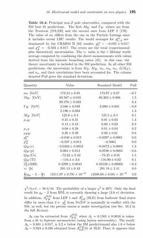
10. Electroweak model and constraints on new physics 195
Table 10.4: Principal non-Z pole observables, compared with theSM best fit predictions. The first MW and ΓW values are fromthe Tevatron [219,220] and the second ones from LEP 2 [170].The value of mt differs from the one in the Particle Listings sinceit includes recent LHC results. The world averages for gνe
V,A are
dominated by the CHARM II [82] results, gνeV = −0.035 ± 0.017
and gνeA = −0.503 ± 0.017. The errors are the total (experimental
plus theoretical) uncertainties. The ττ value is the τ lifetime worldaverage computed by combining the direct measurements with valuesderived from the leptonic branching ratios [45]; in this case, thetheory uncertainty is included in the SM prediction. In all other SMpredictions, the uncertainty is from MZ , MH , mt, mb, mc, α(MZ),and αs, and their correlations have been accounted for. The columndenoted Pull gives the standard deviations.
Quantity Value Standard Model Pull
mt [GeV] 173.24± 0.95 173.87 ± 0.87 −0.7
MW [GeV] 80.387± 0.016 80.363± 0.006 1.5
80.376± 0.033 0.4
ΓW [GeV] 2.046± 0.049 2.090 ± 0.001 −0.9
2.196± 0.083 1.3
MH [GeV] 125.6 ± 0.4 125.5 ± 0.4 0.1
ργW 0.45 ± 0.31 0.01 ± 0.03 1.4
0.12 ± 0.43 0.00 ± 0.03 0.3
ργZ 0.08 ± 0.28 0.01 ± 0.04 0.2
ρZW 0.30 ± 0.39 0.00 ± 0.01 0.8
gνeV −0.040± 0.015 −0.0397± 0.0001 0.0
gνeA −0.507± 0.014 −0.5064 0.0
QW (e) −0.0403± 0.0053 −0.0473± 0.0003 1.3
QW (p) 0.064± 0.012 0.0708± 0.0003 −0.6
QW (Cs) −72.62± 0.43 −73.25± 0.01 1.5
QW (Tl) −116.4± 3.6 −116.90± 0.02 0.1
s2Z(eDIS) 0.2299± 0.0043 0.23126± 0.00005 −0.3
ττ [fs] 291.13± 0.43 291.19 ± 2.41 0.0
12 (gµ − 2 − α
π ) (4511.07± 0.79) × 10−9 (4508.68± 0.08) × 10−9 3.0
χ2/d.o.f. = 48.3/44. The probability of a larger χ2 is 30%. Only the finalresult for gµ − 2 from BNL is currently showing a large (3.0 σ) deviation.
In addition, A(0,b)FB from LEP 1 and A0
LR (SLD) from hadronic final states
differ by more than 2 σ. g2L from NuTeV is nominally in conflict with the
SM, as well, but the precise status is under investigation (see Sec. 10.3 inthe full Review).
Ab can be extracted from A(0,b)FB when Ae = 0.1501 ± 0.0016 is taken
from a fit to leptonic asymmetries (using lepton universality). The result,Ab = 0.881 ± 0.017, is 3.2 σ below the SM predictionand also 1.6 σ belowAb = 0.923 ± 0.020 obtained from AFB
LR (b) at SLD. Thus, it appears that
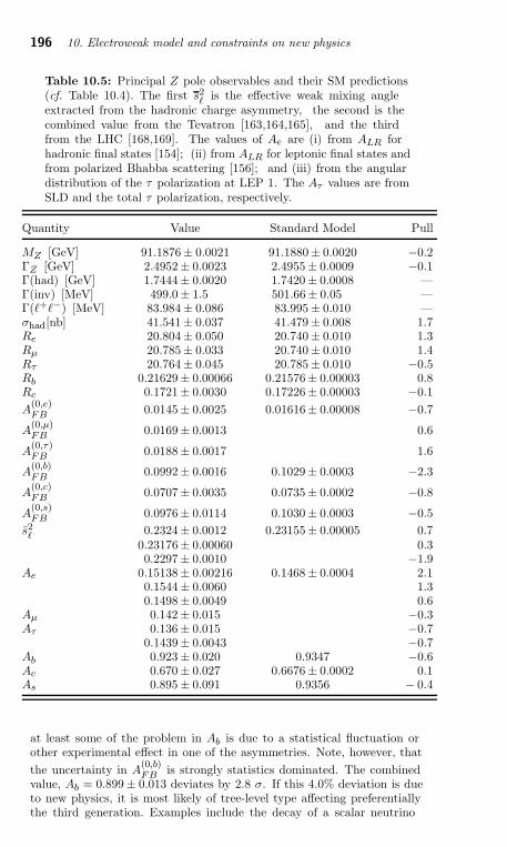
196 10. Electroweak model and constraints on new physics
Table 10.5: Principal Z pole observables and their SM predictions(cf. Table 10.4). The first s2
ℓ is the effective weak mixing angleextracted from the hadronic charge asymmetry, the second is thecombined value from the Tevatron [163,164,165], and the thirdfrom the LHC [168,169]. The values of Ae are (i) from ALR forhadronic final states [154]; (ii) from ALR for leptonic final states andfrom polarized Bhabba scattering [156]; and (iii) from the angulardistribution of the τ polarization at LEP 1. The Aτ values are fromSLD and the total τ polarization, respectively.
Quantity Value Standard Model Pull
MZ [GeV] 91.1876± 0.0021 91.1880± 0.0020 −0.2ΓZ [GeV] 2.4952± 0.0023 2.4955± 0.0009 −0.1Γ(had) [GeV] 1.7444± 0.0020 1.7420± 0.0008 —Γ(inv) [MeV] 499.0 ± 1.5 501.66± 0.05 —Γ(ℓ+ℓ−) [MeV] 83.984 ± 0.086 83.995± 0.010 —σhad[nb] 41.541 ± 0.037 41.479± 0.008 1.7Re 20.804 ± 0.050 20.740± 0.010 1.3Rµ 20.785 ± 0.033 20.740± 0.010 1.4Rτ 20.764 ± 0.045 20.785± 0.010 −0.5Rb 0.21629± 0.00066 0.21576± 0.00003 0.8Rc 0.1721± 0.0030 0.17226± 0.00003 −0.1
A(0,e)FB 0.0145± 0.0025 0.01616± 0.00008 −0.7
A(0,µ)FB 0.0169± 0.0013 0.6
A(0,τ)FB 0.0188± 0.0017 1.6
A(0,b)FB
0.0992± 0.0016 0.1029± 0.0003 −2.3
A(0,c)FB 0.0707± 0.0035 0.0735± 0.0002 −0.8
A(0,s)FB 0.0976± 0.0114 0.1030± 0.0003 −0.5
s2ℓ 0.2324± 0.0012 0.23155± 0.00005 0.7
0.23176± 0.00060 0.30.2297± 0.0010 −1.9
Ae 0.15138± 0.00216 0.1468± 0.0004 2.10.1544± 0.0060 1.30.1498± 0.0049 0.6
Aµ 0.142 ± 0.015 −0.3Aτ 0.136 ± 0.015 −0.7
0.1439± 0.0043 −0.7Ab 0.923 ± 0.020 0.9347 −0.6Ac 0.670 ± 0.027 0.6676± 0.0002 0.1As 0.895 ± 0.091 0.9356 − 0.4
at least some of the problem in Ab is due to a statistical fluctuation orother experimental effect in one of the asymmetries. Note, however, that
the uncertainty in A(0,b)FB is strongly statistics dominated. The combined
value, Ab = 0.899 ± 0.013 deviates by 2.8 σ. If this 4.0% deviation is dueto new physics, it is most likely of tree-level type affecting preferentiallythe third generation. Examples include the decay of a scalar neutrino
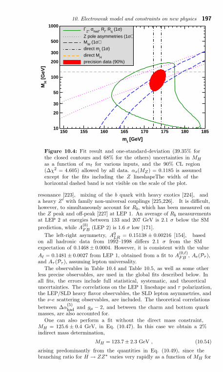
10. Electroweak model and constraints on new physics 197
150 155 160 165 170 175 180 185
mt [GeV]
10
20
30
50
100
200
300
500
1000
MH [G
eV]
ΓZ, σhad, Rl, Rq (1σ)
Z pole asymmetries (1σ)MW (1σ)direct mt (1σ)
direct MH
precision data (90%)
Figure 10.4: Fit result and one-standard-deviation (39.35% forthe closed contours and 68% for the others) uncertainties in MH
as a function of mt for various inputs, and the 90% CL region(∆χ2 = 4.605) allowed by all data. αs(MZ) = 0.1185 is assumedexcept for the fits including the Z lineshapeThe width of thehorizontal dashed band is not visible on the scale of the plot.
resonance [223], mixing of the b quark with heavy exotics [224], anda heavy Z ′ with family non-universal couplings [225,226]. It is difficult,however, to simultaneously account for Rb, which has been measured onthe Z peak and off-peak [227] at LEP 1. An average of Rb measurementsat LEP 2 at energies between 133 and 207 GeV is 2.1 σ below the SM
prediction, while A(b)FB (LEP 2) is 1.6 σ low [171].
The left-right asymmetry, A0LR = 0.15138 ± 0.00216 [154], based
on all hadronic data from 1992–1998 differs 2.1 σ from the SMexpectation of 0.1468 ± 0.0004. However, it is consistent with the value
Aℓ = 0.1481 ± 0.0027 from LEP 1, obtained from a fit to A(0,ℓ)FB , Ae(Pτ ),
and Aτ (Pτ ), assuming lepton universality.
The observables in Table 10.4 and Table 10.5, as well as some otherless precise observables, are used in the global fits described below. Inall fits, the errors include full statistical, systematic, and theoreticaluncertainties. The correlations on the LEP 1 lineshape and τ polarization,the LEP/SLD heavy flavor observables, the SLD lepton asymmetries, andthe ν-e scattering observables, are included. The theoretical correlations
between ∆α(5)had and gµ − 2, and between the charm and bottom quark
masses, are also accounted for.
One can also perform a fit without the direct mass constraint,MH = 125.6 ± 0.4 GeV, in Eq. (10.47). In this case we obtain a 2%indirect mass determination,
MH = 123.7± 2.3 GeV , (10.54)
arising predominantly from the quantities in Eq. (10.49), since thebranching ratio for H → ZZ∗ varies very rapidly as a function of MH for
198 10. Electroweak model and constraints on new physics
Higgs masses near 125 GeV. Removing also the branching ratio constraintsgives the loop-level determination from the precision data alone,
MH = 89+22−18 GeV , (10.55)
which is 1.5 σ below the kinematical constraint. This is mostly a reflectionof the Tevatron determination of MW , which is 1.5 σ higher than the SMbest fit value in Table 10.4. Another consequence is that the 90% centralconfidence range determined from the precision data,
60 GeV < MH < 127 GeV , (10.56)
is only marginally consistent with Eq. (10.47), see Fig. 10.4.
The extracted Z pole value of αs(MZ) is based on a formula withnegligible theoretical uncertainty if one assumes the exact validityof the SM. One should keep in mind, however, that this value,αs(MZ) = 0.1197±0.0027, is very sensitive to certain types of new physicssuch as non-universal vertex corrections. In contrast, the value derivedfrom τ decays, αs(MZ) = 0.1193+0.0022
−0.0020, is theory dominated but lesssensitive to new physics. The two values are in remarkable agreement witheach other. They are also in perfect agreement with the averages from jet-event shapes in e+e− annihilation (0.1177±0.0046) and lattice simulations(0.1185± 0.0005), whereas the DIS average (0.1154± 0.0020) is somewhatlower. For more details, see Section 9 on “Quantum Chromodynamics” inthis Review.
10.7. Constraints on new physics
The masses and decay properties of the electroweak bosons and lowenergy data can be used to search for and set limits on deviations fromthe SM. We will mainly discuss the effects of exotic particles (withheavy masses Mnew ≫ MZ in an expansion in MZ/Mnew) on the gaugeboson self-energies. Most of the effects on precision measurements can bedescribed by three gauge self-energy parameters S, T , and U . We willdefine these, as well as the related parameter ρ0, to arise from new physicsonly. In other words, they are equal to zero (ρ0 = 1) exactly in the SM,and do not include any (loop induced) contributions that depend on mt orMH , which are treated separately.
The dominant effect of many extensions of the SM can be described bythe ρ0 parameter,
ρ0 ≡M2
W
M2Z c 2
Z ρ, (10.57)
which describes new sources of SU(2) breaking that cannot be accountedfor by the SM Higgs doublet or mt effects. From the global fit,
ρ0 = 1.00040± 0.00024 . (10.58)
The result in Eq. (10.58) is 1.7 σ above the SM expectation, ρ0 = 1.It can be used to constrain higher-dimensional Higgs representations tohave vacuum expectation values of less than a few percent of those of thedoublets. Furthermore, it implies the following limit on the mass splitting,∆m2
i , of all new scalar or fermion SU(2) doublets at the 95% CL,
∑
i
Ci
3∆m2
i ≤ (50 GeV)2. (10.63)
where the sum runs over all new-physics doublets, and C = 1 (3) for colorsinglets (triplets).
10. Electroweak model and constraints on new physics 199
A number of authors [236–241] have considered the general effects onneutral-current and Z and W boson observables of various types of heavy(i.e., Mnew ≫ MZ) physics which contribute to the W and Z self-energiesbut which do not have any direct coupling to the ordinary fermions.Such effects can be described by just three parameters, S, T , and U .
Denoting the contributions of new physics to the various self-energies byΠnew
ij , we have
α(MZ)T ≡Πnew
WW (0)
M2W
−Πnew
ZZ (0)
M2Z
, (10.64a)
α(MZ)
4 s 2Z c 2
Z
S ≡Πnew
ZZ (M2Z) − Πnew
ZZ (0)
M2Z
−
c 2Z − s 2
Z
c Z s Z
ΠnewZγ (M2
Z)
M2Z
−Πnew
γγ (M2Z)
M2Z
, (10.64b)
α(MZ)
4 s 2Z
(S + U) ≡Πnew
WW (M2W ) − Πnew
WW (0)
M2W
−
c Z
s Z
ΠnewZγ (M2
Z)
M2Z
−Πnew
γγ (M2Z)
M2Z
. (10.64c)
S, T , and U are defined with a factor proportional to α removed, so thatthey are expected to be of order unity in the presence of new physics.A heavy non-degenerate multiplet of fermions or scalars contributespositively to T , which is related to the ρ0 parameter via ρ0−1 ≃ α(MZ)T .A heavy degenerate ordinary or mirror family would contribute 2/3π to S.Large positive values S > 0 can also be generated in Technicolor modelswith QCD-like dynamics, and in models with warped extra dimensions.
The data allow a simultaneous determination of s 2Z (from the Z pole
asymmetries), S (from MZ), U (from MW ), T (mainly from ΓZ), αs (fromRℓ, σhad, and ττ ), MH and mt (from the hadron colliders), with littlecorrelation among the SM parameters:
S = −0.03 ± 0.10, T = 0.01 ± 0.12, U = 0.05 ± 0.10, (10.70)
s 2Z = 0.23119 ± 0.00016, and αs(MZ) = 0.1196 ± 0.0017, where the
uncertainties are from the inputs. The parameters in Eqs. (10.70), whichby definition are due to new physics only, are in excellent agreement withthe SM values of zero. There is a strong correlation (90%) between theS and T parameters. The U parameter is −59% (−81%) anti-correlatedwith S (T ).
More examples for constraints on new physics can be found in the fullReview.
Further discussion and all references may be found in the full Review
of Particle Physics; the equation and reference numbering corresponds tothat version.
200 11. Status of Higgs boson physics
11. STATUS OF HIGGS BOSON PHYSICS
Written November 2013 by M. Carena (FNAL and the Universityof Chicago), C. Grojean (ICREA at IFAE, Universitat Autonoma deBarcelona), M. Kado (Laboratoire de l’Accelerateur Lineaire, LAL andCERN), and V. Sharma (UC San Diego).
I. Introduction
The observation by ATLAS [1] and CMS [2] of a new boson with amass of approximately 125GeV decaying into γγ, WW and ZZ bosonsand the subsequent studies of the properties of this particle is a milestonein the understanding of the mechanism that breaks electroweak symmetryand generates the masses of the known elementary particles (In thecase of neutrinos, it is possible that the EWSB mechanism plays only apartial role in generating the observed neutrino masses, with additionalcontributions at a higher scale via the so called see-saw mechanism.), oneof the most fundamental problems in particle physics.
In the Standard Model, the mechanism of electroweak symmetrybreaking (EWSB) [3] provides a general framework to keep untouched thestructure of the gauge interactions at high energy and still generate theobserved masses of the W and Z gauge bosons by means of charged andneutral Goldstone bosons that manifest themselves as the longitudinalcomponents of the gauge bosons. The discovery of ATLAS and CMS nowstrongly suggests that these three Goldstone bosons combine with an extra(elementary) scalar boson to form a weak doublet.
This picture matches very well with the Standard Model (SM) [4]which describes the electroweak interactions by a gauge field theoryinvariant under the SU(2)
L× U(1)
Ysymmetry group. In the SM, the
EWSB mechanism posits a self-interacting complex doublet of scalarfields, and the renormalizable interactions are arranged such that theneutral component of the scalar doublet acquires a vacuum expectationvalue (VEV) v ≈ 246GeV, which sets the scale of electroweak symmetrybreaking.
Three massless Goldstone bosons are generated, which are absorbed togive masses to the W and Z gauge bosons. The remaining component ofthe complex doublet becomes the Higgs boson – a new fundamental scalarparticle. The masses of all fermions are also a consequence of EWSB sincethe Higgs doublet is postulated to couple to the fermions through Yukawainteractions. However, the true structure behind the newly discoveredboson, including the exact dynamics that triggers the Higgs VEV, and thecorresponding ultraviolet completion is still unsolved.
Even if the discovered boson has weak couplings to all known SMdegrees of freedom, it is not impossible that it is part of an extendedsymmetry structure or that it emerges from a light resonance of a stronglycoupled sector. It needs to be established whether the Higgs boson issolitary or whether other states populate the EWSB sector.
Further discussion and references may be found in the full Review of
Particle Physics.
12. The CKM quark-mixing matrix 201
12. THE CKM QUARK-MIXING MATRIX
Revised February 2014 by A. Ceccucci (CERN), Z. Ligeti (LBNL), andY. Sakai (KEK).
12.1. Introduction
The masses and mixings of quarks have a common origin in theStandard Model (SM). They arise from the Yukawa interactions of thequarks with the Higgs condensate. When the Higgs field acquires a vacuumexpectation value, quark mass terms are generated. The physical states areobtained by diagonalizing the up and down quark mass matrices by four
unitary matrices, Vu,dL,R. As a result, the charged current W± interactions
couple to the physical up and down-type quarks with couplings given by
VCKM ≡ V uL V
d†L =
Vud Vus VubVcd Vcs VcbVtd Vts Vtb
. (12.2)
This Cabibbo-Kobayashi-Maskawa (CKM) matrix [1,2] is a 3 × 3unitary matrix. It can be parameterized by three mixing angles and aCP -violating phase,
V =
c12
c13
s12
c13
s13
e−iδ
−s12
c23−c
12s23
s13
eiδ c12
c23−s
12s23
s13
eiδ s23
c13
s12
s23−c
12c23
s13
eiδ −c12
s23−s
12c23
s13
eiδ c23
c13
, (12.3)
where sij = sin θij , cij = cos θij , and δ is the phase responsible for allCP -violating phenomena in flavor changing processes in the SM. Theangles θij can be chosen to lie in the first quadrant.
It is known experimentally that s13 ≪ s23 ≪ s12 ≪ 1, and it isconvenient to exhibit this hierarchy using the Wolfenstein parameterization.We define [4–6]
s12 = λ =|Vus|
√
|Vud|2 + |Vus|2, s23 = Aλ2 = λ
∣
∣
∣
∣
Vcb
Vus
∣
∣
∣
∣
,
s13eiδ = V ∗
ub = Aλ3(ρ + iη) =Aλ3(ρ + iη)
√1 − A2λ4
√1 − λ2[1 − A2λ4(ρ + iη)]
. (12.4)
These ensure that ρ + iη = −(VudV∗ub)/(VcdV ∗
cb) is phase-conventionindependent and the CKM matrix written in terms of λ, A, ρ and η isunitary to all orders in λ. To O(λ4),
V =
1 − λ2/2 λ Aλ3(ρ − iη)−λ 1 − λ2/2 Aλ2
Aλ3(1 − ρ − iη) −Aλ2 1
+ O(λ4) . (12.5)
Unitarity implies∑
i VijV∗ik = δjk and
∑
j VijV∗kj = δik. The six
vanishing combinations can be represented as triangles in a complex plane.The most commonly used unitarity triangle arises from
Vud V ∗ub + Vcd V ∗
cb + Vtd V ∗tb = 0 , (12.6)
by dividing each side by VcdV∗cb (see Fig. 1). The vertices are exactly (0, 0),
(1, 0) and, due to the definition in Eq. (12.4), (ρ, η). An important goal offlavor physics is to overconstrain the CKM elements, many of which canbe displayed and compared in the ρ, η plane.
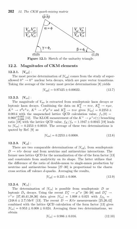
202 12. The CKM quark-mixing matrix
Figure 12.1: Sketch of the unitarity triangle.
12.2. Magnitudes of CKM elements
12.2.1. |Vud| :
The most precise determination of |Vud| comes from the study of super-allowed 0+ → 0+ nuclear beta decays, which are pure vector transitions.Taking the average of the twenty most precise determinations [8] yields
|Vud| = 0.97425± 0.00022. (12.7)
12.2.2. |Vus| :
The magnitude of Vus is extracted from semileptonic kaon decays orleptonic kaon decays. Combining the data on K0
L → πeν, K0L → πµν,
K± → π0e±ν, K± → π0µ±ν and K0S → πeν gives |Vus| = 0.2253 ±
0.0014 with the unquenched lattice QCD calculation value, f+(0) =0.960+0.005
−0.006 [12]. The KLOE measurement of the K+ → µ+ν(γ) branchingratio [18] with the lattice QCD value, fK/fπ = 1.1947 ± 0.0045 [19] leadsto |Vus| = 0.2253 ± 0.0010. The average of these two determinations isquoted by Ref. [9] as
|Vus| = 0.2253± 0.0008. (12.8)
12.2.3. |Vcd| :
There are two comparable determinations of |Vcd|, from semileptonicD → πℓν decay and from neutrino and antineutrino interactions. Theformer uses lattice QCD for the normalization of the of the form factor [13]and constraints from analyticity on its shape. The latter utilizes thatthe difference of the ratio of double-muon to single-muon production byneutrino and antineutrino beams [27–30] is proportional to the charmcross section off valence d-quarks. Averaging the results,
|Vcd| = 0.225± 0.008. (12.9)
12.2.4. |Vcs| :
The determination of |Vcs| is possible from semileptonic D orleptonic Ds decays. Using the recent D+
s → µ+ν [36–38] and D+s →
τ+ν [37,40,41,38,36] data gives |Vcs| = 1.008 ± 0.021 with fDs=
(248.6 ± 2.7)MeV [13]. The recent D → Kℓν measurements [25,26,42]combined with the lattice QCD calculation of the form factor [13] gives|Vcs| = 0.953 ± 0.008 ± 0.024. Averaging these two determinations, weobtain
|Vcs| = 0.986 ± 0.016. (12.10)
12. The CKM quark-mixing matrix 203
12.2.5. |Vcb| :
The determination of |Vcb| from inclusive semileptonic B decays usethe semileptonic rate measurement together with the leptonic energyand the hadronic invariant-mass spectra. Determinations from exclusiveB → D(∗)ℓν decays are based on the fact that in the mb,c ≫ ΛQCD limitall form factors are given by a single Isgur-Wise function [49], which isnormalized at zero recoil. The Vcb and Vub minireview [14] quotes thecombination with a scaled error as
|Vcb| = (41.1 ± 1.3) × 10−3. (12.11)
12.2.6. |Vub| :
The determination of |Vub| from inclusive B → Xuℓν decay suffers fromlarge B → Xcℓν backgrounds. In most regions of phase space where thecharm background is kinematically forbidden the rate is determined bynonperturbative shape functions. At leading order in ΛQCD/mb there isonly one such function, which is related to the photon energy spectrumin B → Xsγ [51,52]. The large and pure BB samples at the B factoriespermit the selection of B → Xuℓν decays in events where the other B isfully reconstructed [57]. With this full-reconstruction tag method, one canmeasure the four-momenta of both the leptonic and hadronic systems, andaccess wider kinematic regions because of improved signal purity.
To extract |Vub| from exclusive channels, the form factors have to beknown. Unquenched lattice QCD calculations of the B → πℓν form factorfor q2 > 16 GeV2 are available [58,59]. The theoretical uncertainties inthe inclusive and exclusive determinations are different. The Vcb and Vubminireview [14] quotes the combination
|Vub| = (4.13 ± 0.49)× 10−3. (12.12)
12.2.7. |Vtd| and |Vts| :
These CKM elements are not likely to be precisely measurablein tree-level processes involving top quarks, so one has to use B–Boscillations or loop-mediated rare K and B decays. The mass differenceof the two neutral B meson mass eigenstates is well measured,∆md = (0.510 ± 0.003)ps−1 [62]. In the B0
s system, the averageof the CDF [63] and recent more precise LHCb [64] measurementsyields ∆ms = (17.761 ± 0.022) ps−1. Using unquenched lattice QCDcalculations [13] and assuming |Vtb| = 1, we find
|Vtd| = (8.4 ± 0.6) × 10−3, |Vts| = (40.0 ± 2.7) × 10−3. (12.13)
Several uncertainties are reduced in the lattice QCD calculation of theratio ∆md/∆ms, which gives a significantly improved constraint,
∣
∣Vtd/Vts∣
∣ = 0.216± 0.001 ± 0.011. (12.14)
12.2.8. |Vtb| :
The determination of |Vtb| from top decays uses the ratio of branchingfractions B(t → Wb)/B(t → Wq) = |Vtb|2/(
∑
q |Vtq |2) = |Vtb|2, where
q = b, s, d [73–75]. The direct determination of |Vtb| without assumingunitarity has become possible from the single top quark production crosssection. The (3.51+0.40
−0.37) pb average Tevatron cross section [76,77] implies|Vtb| = 1.03 ± 0.06. The average t-channel single-top cross section at the
204 12. The CKM quark-mixing matrix
LHC at 7TeV, (68.5 ± 5.8) pb [78,79], implies |Vtb| = 1.03 ± 0.05; theaverage cross section at 8TeV from a subset of the data, (85 ± 12) pb [80],implies |Vtb| = 0.99 ± 0.07. The average of these results gives
|Vtb| = 1.021 ± 0.032 . (12.15)
12.3. Phases of CKM elements
The angles of the unitarity triangle are
β = φ1 = arg
(
−VcdV∗cb
VtdV ∗tb
)
, α = φ2 = arg
(
− VtdV ∗tb
VudV∗ub
)
,
γ = φ3 = arg
(
−VudV ∗ub
VcdV ∗cb
)
. (12.16)
Since CP violation involves phases of CKM elements, many measurementsof CP -violating observables can be used to constrain these angles and theρ, η parameters.
12.3.1. ǫ and ǫ′ :
The measurement of CP violation in K0–K0 mixing, |ǫ| = (2.233 ±0.015) × 10−3 [82], provides constraints in the ρ, η plane bounded byhyperbolas approximately. The dominant uncertainties are due to the bagparameter and the parametric uncertainty proportional to σ(A4) [i.e.,σ(|Vcb|4)].
The measurement of ǫ′ provides a qualitative test of the CKMmechanism because its nonzero experimental average, Re(ǫ′/ǫ) =(1.67 ± 0.23) × 10−3 [82], demonstrated the existence of direct CPviolation, a prediction of the KM ansatz. While Re(ǫ′/ǫ) ∝ Im(VtdV ∗
ts),this quantity cannot easily be used to extract CKM parameters, becauseof hadronic uncertainties.
12.3.2. β / φ1 :
The time-dependent CP asymmetry of neutral B decays to a final statef common to B0 and B0 is given by [92,93]
Af =Γ(B0(t) → f) − Γ(B0(t) → f)
Γ(B0(t) → f) + Γ(B0(t) → f)= Sf sin(∆m t) − Cf cos(∆m t),
(12.18)where Sf = 2 Imλf/(1 + |λf |2), Cf = (1 − |λf |2)/(1 + |λf |2), and
λf = (q/p)(Af/Af ). Here q/p describes B0–B0 mixing and, to a good
approximation in the SM, q/p = V ∗tbVtd/VtbV
∗td = e−2iβ+O(λ4) in the usual
phase convention. Af (Af ) is the amplitude of B0 → f (B0 → f) decay.If f is a CP eigenstate and amplitudes with one CKM phase dominate,then |Af | = |Af |, Cf = 0 and Sf = sin(arg λf ) = ηf sin 2φ, where ηf is
the CP eigenvalue of f and 2φ is the phase difference between the B0 → fand B0 → B0 → f decay paths.
The b → ccs decays to CP eigenstates (B0 → charmonium K0S,L)
are the theoretically cleanest examples, measuring Sf = −ηf sin 2β. Theworld average is [98]
sin 2β = 0.682 ± 0.019 . (12.20)
This measurement of β has a four-fold ambiguity. Of these, β → π/2 − β(but not β → π + β) has been resolved by a time-dependent angular
12. The CKM quark-mixing matrix 205
analysis of B0 → J/ψK∗0 [99,100] and a time-dependent Dalitz plotanalysis of B0 → D0h0 (h0 = π0, η, ω) [101,102].
The b → sqq penguin dominated decays have the same CKM phaseas the b → ccs tree dominated decays, up to corrections suppressedby λ2. Therefore, decays such as B0 → φK0 and η′K0 provide sin 2βmeasurements in the SM. If new physics contributes to the b → sloop diagrams and has a different weak phase, it would give rise toSf 6= −ηf sin 2β and possibly Cf 6= 0. The results and their uncertaintiesare summarized in Fig. 12.3 and Table 12.1 of Ref. [93].
12.3.3. α / φ2 :
Since α is the phase between V ∗tbVtd and V ∗
ubVud, only time-dependentCP asymmetries in b → uud dominated modes can directly measure it.In such decays the penguin contribution can be sizable. Then Sπ+π− nolonger measures sin 2α, but α can still be extracted using the isospinrelations among the B0 → π+π−, B0 → π0π0, and B+ → π+π0
amplitudes and their CP conjugates [103]. Because the isospin analysisgives 16 mirror solutions, only a loose constraint is obtained at present.
The B0 → ρ+ρ− decay can in general have a mixture of CP -even andCP -odd components. However, the longitudinal polarization fractions inB+ → ρ+ρ0 and B0 → ρ+ρ− are measured to be close to unity [106], whichimplies that the final states are almost purely CP -even. Furthermore,B(B0 → ρ0ρ0) = (0.97±0.24)×10−6 implies that the effect of the penguindiagrams is small. The isospin analysis gives α = (89.9 ± 5.4) [105] witha mirror solution at 3π/2 − α.
The final state in B0 → ρ+π− decay is not a CP eigenstate, butmixing induced CP violations can still occur in the four decay amplitudes,B0,B0 → ρ±π∓. Because of the more complicated isospin relations, thetime-dependent Dalitz plot analysis of B0 → π+π−π0 gives the best modelindependent extraction of α [109]. The combination of Belle [110] andBABAR [111] measurements yield α = (54.1+7.7
−10.3) and (141.8+4.7
−5.4) [105].
Combining these three decay modes [105], α is constrained as
α = (85.4+3.9−3.8)
. (12.23)
12.3.4. γ / φ3 :
The angle γ does not depend on CKM elements involving the topquark, so it can be measured in tree-level B decays. This is an importantdistinction from α and β, implying that the measurements of γ are unlikelyto be affected by physics beyond the SM.
The interference of B− → D0K− (b → cus) and B− → D0K−
(b → ucs) transitions can be studied in final states accessible in bothD0 and D0 decays [92]. It is possible to extract from the data the Band D decay amplitudes, their relative strong phases, and γ. Analyses intwo-body D decays using the GLW [113,114] and ADS methods [115] havebeen made by the B factories [116,117], CDF [118], and LHCb [119]. TheDalitz plot analysis of D0, D0 → KSπ+π− [120,121] by the B factoriesgives the best present determination of γ [122,123].
Combining these analyses [105],
γ = (68.0+8.0−8.5)
. (12.25)
206 12. The CKM quark-mixing matrix
12.4. Global fit in the Standard Model
Using the independently measured CKM elements mentioned inthe previous sections, the unitarity of the CKM matrix can bechecked. We obtain |Vud|2 + |Vus|2 + |Vub|2 = 0.9999 ± 0.0006 (1st row),|Vcd|2 + |Vcs|2 + |Vcb|2 = 1.024± 0.032 (2nd row), |Vud|2 + |Vcd|2 + |Vtd|2 =1.000 ± 0.004 (1st column), and |Vus|2 + |Vcs|2 + |Vts|2 = 1.025 ± 0.032(2nd column), respectively. For the second row, a more stringent checkis obtained subtracting the sum of the first row from the measurementof
∑
u,c,d,s,b |Vij |2 from the W leptonic branching ratio [43], yielding
|Vcd|2 + |Vcs|2 + |Vcb|2 = 1.002 ± 0.027. The sum of the three angles,α + β + γ = (175 ± 9), is also consistent with the SM expectation.
The CKM matrix elements can be most precisely determined by aglobal fit that uses all available measurements and imposes the SMconstraints. There are several approaches to combining the experimentaldata [6,105,112,133], which provide similar results. The results for theWolfenstein parameters are
λ = 0.22537± 0.00061 , A = 0.814+0.023−0.024 ,
ρ = 0.117 ± 0.021 , η = 0.353± +0.013 . (12.26)
The allowed ranges of the magnitudes of all nine CKM elements are
VCKM =
0.97427± 0.00014 0.22536± 0.00061 0.00355± 0.000150.22522± 0.00061 0.97343± 0.00015 0.0414± 0.00120.00886+0.00033
−0.00032 0.0405+0.0011−0.0012 0.99914± 0.00005
,
(12.27)and the Jarlskog invariant is J = (3.06+0.21
−0.20) × 10−5. Fig. 12.2 illustratesthe constraints on the ρ, η plane from various measurements and the globalfit result. The shaded 95% CL regions all overlap consistently around theglobal fit region.
12.5. Implications beyond the SM
The effects in B, K, and D decays and mixings due to high-scale physics(W , Z, t, h in the SM, or new physics particles) can be parameterized byoperators composed of SM fields, obeying the SU(3)×SU(2)×U(1) gaugesymmetry. The observable effects of non-SM interactions are encodedin the coefficients of these operators, and are suppressed by powers ofthe new physics scale. In the SM, these coefficients are determined byjust the four CKM parameters, and the W , Z, and quark masses. Forexample, ∆md, Γ(B → ργ), and Γ(B → Xdℓ
+ℓ−) are all proportionalto |VtdV ∗
tb|2 in the SM, however, they may receive unrelated newphysics contributions. Similar to measurements of sin 2β in tree- andloop-dominated decays, overconstraining the magnitudes and phases offlavor-changing neutral-current amplitudes give good sensitivity to newphysics.
To illustrate the level of suppression required for non-SM contributions,consider a class of models in which the dominant effect of new physics is tomodify the neutral meson mixing amplitudes [136] by (zij/Λ2)(qiγ
µPLqj)2.
New physics with a generic weak phase may still contribute to mesonmixings at a significant fraction of the SM [141,133]. The data imply that
Λ/|zij|1/2 has to exceed about 104 TeV for K0 –K0 mixing, 103 TeV for
D0 – D0 mixing, 500TeV for B0 –B0 mixing, and 100TeV for B0s –B0
smixing [133,138]. Thus, if there is new physics at the TeV scale, |zij | ≪ 1
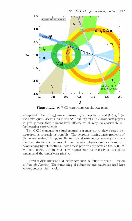
12. The CKM quark-mixing matrix 207
γ
γ
αα
dm∆Kε
Kε
sm∆ & dm∆
ubV
βsin 2
(excl. at CL > 0.95) < 0βsol. w/ cos 2
excluded at CL > 0.95
α
βγ
ρ-1.0 -0.5 0.0 0.5 1.0 1.5 2.0
η
-1.5
-1.0
-0.5
0.0
0.5
1.0
1.5excluded area has CL > 0.95
Figure 12.2: 95% CL constraints on the ρ, η plane.
is required. Even if |zij | are suppressed by a loop factor and |V ∗tiVtj |2 (in
the down quark sector), as in the SM, one expects TeV-scale new physicsto give greater than percent-level effects, which may be observable inforthcoming experiments.
The CKM elements are fundamental parameters, so they should bemeasured as precisely as possible. The overconstraining measurements ofCP asymmetries, mixing, semileptonic, and rare decays severely constrainthe magnitudes and phases of possible new physics contributions toflavor-changing interactions. When new particles are seen at the LHC, itwill be important to know the flavor parameters as precisely as possible tounderstand the underlying physics.
Further discussion and all references may be found in the full Review
of Particle Physics. The numbering of references and equations used herecorresponds to that version.
208 13. CP violation in the quark sector
13. CP VIOLATION IN THE QUARK SECTOR
Revised February 2014 by T. Gershon (University of Warwick) and Y. Nir(Weizmann Institute).
The CP transformation combines charge conjugation C with parityP . Under C, particles and antiparticles are interchanged, by conjugatingall internal quantum numbers, e.g., Q → −Q for electromagnetic charge.Under P , the handedness of space is reversed, ~x → −~x. Thus, for example,a left-handed electron e−L is transformed under CP into a right-handed
positron, e+
R.
If CP were an exact symmetry, the laws of Nature would be the samefor matter and for antimatter. We observe that most phenomena areC- and P -symmetric, and therefore, also CP -symmetric. In particular,these symmetries are respected by the gravitational, electromagnetic, andstrong interactions. The weak interactions, on the other hand, violateC and P in the strongest possible way. For example, the charged Wbosons couple to left-handed electrons, e−L , and to their CP -conjugate
right-handed positrons, e+
R, but to neither their C-conjugate left-handed
positrons, e+
L , nor their P -conjugate right-handed electrons, e−R. Whileweak interactions violate C and P separately, CP is still preserved inmost weak interaction processes. The CP symmetry is, however, violatedin certain rare processes, as discovered in neutral K decays in 1964 [1],and observed in recent years in B decays. A KL meson decays more oftento π−e+νe than to π+e−νe, thus allowing electrons and positrons to beunambiguously distinguished, but the decay-rate asymmetry is only atthe 0.003 level. The CP -violating effects observed in the B system arelarger: the parameter describing the CP asymmetry in the decay time
distribution of B0/B0
meson transitions to CP eigenstates like J/ψKS is
about 0.7 [2,3]. These effects are related to K0−K0
and B0−B0
mixing,but CP violation arising solely from decay amplitudes has also beenobserved, first in K → ππ decays [4–6], and more recently in B0 [7,8],B+ [9–11], and B0
s [12] decays. CP violation is not yet experimentallyestablished in the D system. Moreover, CP violation has not yet beenobserved in the decay of any baryon, nor in processes involving the topquark, nor in flavor-conserving processes such as electric dipole moments,nor in the lepton sector.
In addition to parity and to continuous Lorentz transformations,there is one other spacetime operation that could be a symmetry of theinteractions: time reversal T , t → −t. Violations of T symmetry havebeen observed in neutral K decays [13]. More recently, exploiting thefact that for neutral B mesons both flavor tagging and CP tagging canbe used [14], T violation has been observed between states that arenot CP -conjugate [15]. Moreover, T violation is expected as a corollaryof CP violation if the combined CPT transformation is a fundamentalsymmetry of Nature [16]. All observations indicate that CPT is indeeda symmetry of Nature. Furthermore, one cannot build a locally Lorentz-invariant quantum field theory with a Hermitian Hamiltonian that violatesCPT . (At several points in our discussion, we avoid assumptions aboutCPT , in order to identify cases where evidence for CP violation relies onassumptions about CPT .)
Within the Standard Model, CP symmetry is broken by complexphases in the Yukawa couplings (that is, the couplings of the Higgs
13. CP violation in the quark sector 209
scalar to quarks). When all manipulations to remove unphysical phasesin this model are exhausted, one finds that there is a single CP -violatingparameter [17]. In the basis of mass eigenstates, this single phaseappears in the 3 × 3 unitary matrix that gives the W -boson couplingsto an up-type antiquark and a down-type quark. (If the StandardModel is supplemented with Majorana mass terms for the neutrinos, theanalogous mixing matrix for leptons has three CP -violating phases.) Thebeautifully consistent and economical Standard-Model description of CPviolation in terms of Yukawa couplings, known as the Kobayashi-Maskawa(KM) mechanism [17], agrees with all measurements to date. (Somemeasurements are in tension with the predictions, and are discussed inmore detail below. Pending verification, the results are not consideredto change the overall picture of agreement with the Standard Model.)Furthermore, one can fit the data allowing new physics contributions toloop processes to compete with, or even dominate over, the StandardModel amplitudes [18,19]. Such an analysis provides model-independentproof that the KM phase is different from zero, and that the matrix ofthree-generation quark mixing is the dominant source of CP violation inmeson decays.
The current level of experimental accuracy and the theoreticaluncertainties involved in the interpretation of the various observationsleave room, however, for additional subdominant sources of CP violationfrom new physics. Indeed, almost all extensions of the Standard Modelimply that there are such additional sources. Moreover, CP violationis a necessary condition for baryogenesis, the process of dynamicallygenerating the matter-antimatter asymmetry of the Universe [20].Despite the phenomenological success of the KM mechanism, it fails (byseveral orders of magnitude) to accommodate the observed asymmetry [21].This discrepancy strongly suggests that Nature provides additional sourcesof CP violation beyond the KM mechanism. (The evidence for neutrinomasses implies that CP can be violated also in the lepton sector. Thissituation makes leptogenesis [22], a scenario where CP -violating phases inthe Yukawa couplings of the neutrinos play a crucial role in the generationof the baryon asymmetry, a very attractive possibility.) The expectationof new sources motivates the large ongoing experimental effort to finddeviations from the predictions of the KM mechanism.
CP violation can be experimentally searched for in a variety ofprocesses, such as hadron decays, electric dipole moments of neutrons,electrons and nuclei, and neutrino oscillations. Hadron decays via theweak interaction probe flavor-changing CP violation. The search forelectric dipole moments may find (or constrain) sources of CP violationthat, unlike the KM phase, are not related to flavor-changing couplings.Following the discovery of the Higgs boson [23,24], searches for CPviolation in the Higgs sector are becoming feasible. Future searches forCP violation in neutrino oscillations might provide further input onleptogenesis.
The present measurements of CP asymmetries provide some ofthe strongest constraints on the weak couplings of quarks. Futuremeasurements of CP violation in K, D, B, and B0
s meson decayswill provide additional constraints on the flavor parameters of theStandard Model, and can probe new physics. In this review, we give theformalism and basic physics that are relevant to present and near futuremeasurements of CP violation in the quark sector.
210 13. CP violation in the quark sector
Before going into details, we list here the observables where CPviolation has been observed at a level above 5σ [25–27]:
• Indirect CP violation in K → ππ and K → πℓν decays, and in theKL → π+π−e+e− decay, is given by
|ǫ| = (2.228 ± 0.011)× 10−3 . (13.1)
• Direct CP violation in K → ππ decays is given by
Re(ǫ′/ǫ) = (1.65 ± 0.26) × 10−3 . (13.2)
• CP violation in the interference of mixing and decay in the tree-dominated b → ccs transitions, such as B0 → ψK0, is given by (weuse K0 throughout to denote results that combine KS and KL modes,but use the sign appropriate to KS):
SψK0 = +0.682± 0.019 . (13.3)
• CP violation in the interference of mixing and decay in various modesrelated to b → qqs (penguin) transitions is given by
Sη′K0 = + 0.63 ± 0.06 , (13.4)
SφK0 = + 0.74 +0.11−0.13 , (13.5)
Sf0K0 = + 0.69 +0.10−0.12 , (13.6)
SK+K−KS= + 0.68 +0.09
−0.10 , (13.7)
• CP violation in the interference of mixing and decay in theB0 → π+π− mode is given by
Sπ+π− = −0.66 ± 0.06 . (13.8)
• Direct CP violation in the B0 → π+π− mode is given by
Cπ+π− = −0.31± 0.05 . (13.9)
• CP violation in the interference of mixing and decay in various modesrelated to b → ccd transitions is given by
Sψπ0 = − 0.93 ± 0.15 , (13.10)
SD+D− = − 0.98 ± 0.17 . (13.11)
SD∗+D∗− = − 0.71 ± 0.09 . (13.12)
• Direct CP violation in the B0 → K−π+ mode is given by
AB0→K−π+ = −0.082± 0.006 . (13.13)
• Direct CP violation in B± → D+K± decays (D+ is the CP -evenneutral D state) is given by
AB+→D+K+ = +0.19± 0.03 . (13.14)
• Direct CP violation in the B0
s → K+π− mode is given by
AB
0s→K+π−
= +0.26± 0.04 . (13.15)
In addition, large CP violation effects have recently been observed incertain regions of the phase space of B± → K+K−K±, π+π−K±,π+π−π± and K+K−π± decays [28,29].
Further discussion and references may be found in the full Review of
Particle Physics.
14. Neutrino mixing 211
14. NEUTRINO MASS, MIXING, AND OSCILLATIONS
Updated May 2014 by K. Nakamura (Kavli IPMU (WPI), U. Tokyo,KEK), and S.T. Petcov (SISSA/INFN Trieste, Kavli IPMU (WPI), U.Tokyo, Bulgarian Academy of Sciences).
I. Massive neutrinos and neutrino mixing. It is a well-establishedexperimental fact that the neutrinos and antineutrinos which take partin the standard charged current (CC) and neutral current (NC) weakinteraction are of three varieties (types) or flavours: electron, νe and νe,muon, νµ and νµ, and tauon, ντ and ντ . The notion of neutrino type orflavour is dynamical: νe is the neutrino which is produced with e+, orproduces an e− in CC weak interaction processes; νµ is the neutrino whichis produced with µ+, or produces µ−, etc. The flavour of a given neutrinois Lorentz invariant.
The experiments with solar, atmospheric, reactor and acceleratorneutrinos have provided compelling evidences for the existence of neutrinooscillations [4,5], transitions in flight between the different flavourneutrinos νe, νµ, ντ (antineutrinos νe, νµ, ντ ), caused by nonzeroneutrino masses and neutrino mixing. The existence of flavour neutrinooscillations implies that if a neutrino of a given flavour, say νµ, withenergy E is produced in some weak interaction process, at a sufficientlylarge distance L from the νµ source the probability to find a neutrinoof a different flavour, say ντ , P (νµ → ντ ; E, L), is different from zero.P (νµ → ντ ; E, L) is called the νµ → ντ oscillation or transition probability.If P (νµ → ντ ; E, L) 6= 0, the probability that νµ will not change intoa neutrino of a different flavour, i.e., the “νµ survival probability”P (νµ → νµ; E, L), will be smaller than one. If only muon neutrinos νµ
are detected in a given experiment and they take part in oscillations, onewould observe a “disappearance” of muon neutrinos on the way from theνµ source to the detector.
Oscillations of neutrinos are a consequence of the presence of flavourneutrino mixing, or lepton mixing, in vacuum. In local quantum fieldtheory, used to construct the Standard Model, this means that the LHflavour neutrino fields νlL(x), which enter into the expression for the leptoncurrent in the CC weak interaction Lagrangian, are linear combinations ofthe fields of three (or more) neutrinos νj , having masses mj 6= 0:
νlL(x) =∑
j
Ulj νjL(x), l = e, µ, τ, (14.1)
where νjL(x) is the LH component of the field of νj possessing a mass mj
and U is the unitary neutrino mixing matrix [1,4,5]. Eq. (14.1) impliesthat the individual lepton charges Ll, l = e, µ, τ , are not conserved.
All compelling neutrino oscillation data can be described assuming3-flavour neutrino mixing in vacuum. The number of massive neutrinosνj , n, can, in general, be bigger than 3, n > 3, if, for instance, thereexist sterile neutrinos and they mix with the flavour neutrinos. From theexisting data, at least 3 of the neutrinos νj , say ν1, ν2, ν3, must be light,m1,2,3 . 1 eV, and must have different masses. At present there are severalexperimental hints for existence of one or two light sterile neutrinos withmasses m4,5 ∼ 1 eV (see the full Review for details).
Being electrically neutral, the neutrinos with definite mass νj can beDirac fermions or Majorana particles [39,40]. The first possibility isrealised when there exists a lepton charge carried by the neutrinos νj ,
212 14. Neutrino mixing
which is conserved by the particle interactions. This could be, e.g., thetotal lepton charge L = Le + Lµ + Lτ : L(νj) = 1, j = 1, 2, 3. In this casethe neutrino νj has a distinctive antiparticle νj : νj differs from νj by thevalue of the lepton charge L it carries, L(νj) = − 1. The massive neutrinosνj can be Majorana particles if no lepton charge is conserved. A massiveMajorana particle χj is identical with its antiparticle χj : χj ≡ χj . On thebasis of the existing neutrino data it is impossible to determine whetherthe massive neutrinos are Dirac or Majorana fermions.
In the case of n neutrino flavours and n massive neutrinos, the n × nunitary neutrino mixing matrix U can be parametrised by n(n − 1)/2Euler angles and n(n + 1)/2 phases. If the massive neutrinos νj are Diracparticles, only (n− 1)(n− 2)/2 phases are physical and can be responsiblefor CP violation in the lepton sector. In this respect the neutrino (lepton)mixing with Dirac massive neutrinos is similar to the quark mixing. Forn = 3 there is just one CP violating phase in U , which is usually called“the Dirac CP violating phase.” CP invariance holds if (in a certainstandard convention) U is real, U∗ = U .
If, however, the massive neutrinos are Majorana fermions, νj ≡ χj , theneutrino mixing matrix U contains n(n− 1)/2 CP violation phases [43,44],i.e., by (n− 1) phases more than in the Dirac neutrino case: in contrast toDirac fields, the massive Majorana neutrino fields cannot “absorb” phases.In this case U can be cast in the form [43]
U = V P (14.2)
where the matrix V contains the (n − 1)(n − 2)/2 Dirac CP violationphases, while P is a diagonal matrix with the additional (n− 1) MajoranaCP violation phases α21, α31,..., αn1,
P = diag(
1, eiα212 , ei
α312 , ..., ei
αn12
)
. (14.3)
The Majorana phases will conserve CP if [45] αj1 = πqj , qj = 0, 1, 2,j = 2, 3, ..., n. In this case exp[i(αj1 −αk1)] = ±1 is the relative CP-parityof Majorana neutrinos χj and χk. The condition of CP invariance of theleptonic CC weak interaction in the case of mixing and massive Majorananeutrinos reads [41]:
U∗lj = Ulj ρj , ρj =
1
iηCP (χj) = ±1 , (14.4)
where ηCP (χj) = iρj = ±i is the CP parity of the Majorana neutrinoχj [45]. If CP invariance holds, the elements of U are either real orpurely imaginary.
In the case of n = 3 there are 3 CP violation phases - one Dirac andtwo Majorana. Even in the mixing involving only 2 massive Majorananeutrinos there is one physical CP violation Majorana phase.
II. Neutrino oscillations in vacuum. Neutrino oscillations are aquantum mechanical consequence of the existence of nonzero neutrinomasses and neutrino (lepton) mixing, Eq. (14.1), and of the relativelysmall splitting between the neutrino masses. Suppose the flavour neutrinoνl is produced in a CC weak interaction process and after a time T it isobserved by a neutrino detector, located at a distance L from the neutrinosource and capable of detecting also neutrinos νl′ , l′ 6= l. If lepton mixing,Eq. (14.1), takes place and the masses mj of all neutrinos νj are sufficientlysmall, the state of the neutrino νl, |νl〉, will be a coherent superposition of
14. Neutrino mixing 213
the states |νj〉 of neutrinos νj :
|νl〉 =∑
j
U∗lj |νj ; pj〉, l = e, µ, τ , (14.5)
where U is the neutrino mixing matrix and pj is the 4-momentum ofνj [47]. For the state vector of RH flavour antineutrino νl, produced in aCC weak interaction process we similarly get:
|νl〉 =∑
j
Ulj |νj ; pj〉 ∼=∑
j=1
Ulj |νj , R; pj〉, l = e, µ, τ. (14.7)
We will assume in what follows that the neutrino mass spectrum isnot degenerate: mj 6= mk, j 6= k. Then the states |νj ; pj〉 in the linearsuperposition in the r.h.s. of Eq. (14.5) will have, in general, differentenergies and different momenta, independently of whether they areproduced in a decay or interaction process: pj 6= pk, or Ej 6= Ek, pj 6= pk,
j 6= k, where Ej =√
p2j + m2
j , pj ≡ |pj |. The deviations of Ej and pj
from the values for a massless neutrino E and p = E are proportional tom2
j/E0, E0 is the characteristic energy of the process, and is very small.
Suppose that the neutrinos are observed via a CC weak interactionprocess and that in the detector’s rest frame they are detected after timeT after emission, after traveling a distance L. Then the amplitude of theprobability that neutrino νl′ will be observed if neutrino νl was producedby the neutrino source can be written as [46,48,50]:
A(νl → νl′) =∑
j
Ul′j Dj U†jl , l, l′ = e, µ, τ , (14.8)
where Dj = Dj(pj ; L, T ) describes the propagation of νj between the
source and the detector, U†jl
and Ul′j are the amplitudes to find νj in the
initial and in the final flavour neutrino state, respectively. It follows fromrelativistic Quantum Mechanics considerations that [46,48]
Dj ≡ Dj(pj ; L, T ) = e−ipj (xf−x0) = e−i(EjT−pjL) , pj ≡ |pj | , (14.9)
where [51] x0 and xf are the space-time coordinates of the points ofneutrino production and detection, T = (tf − t0) and L = k(xf − x0),k being the unit vector in the direction of neutrino momentum,pj = kpj. What is relevant for the calculation of the probability
P (νl → νl′) = |A(νl → νl′)|2 is the interference factor DjD∗k which
depends on the phase
δϕjk = (Ej − Ek)
[
T − Ej + Ek
pj + pkL
]
+m2
j − m2k
pj + pkL . (14.10)
Some authors [52] have suggested that the distance traveled by theneutrinos L and the time interval T are related by T = (Ej + Ek)L/(pj +pk) = L/v, v = (Ej/(Ej + Ek))vj + (Ek/(Ej + Ek))vk being the “average”velocity of νj and νk, where vj,k = pj,k/Ej,k. In this case the first term inthe r.h.s. of Eq. (14.10) vanishes. The indicated relation has not emergedso far from any dynamical wave packet calculations. We arrive at thesame conclusion concerning the term under discussion in Eq. (14.10) if oneassumes [53] that Ej = Ek = E0. Finally, it was proposed in Ref. 50 andRef. 54 that the states of νj and νj in Eq. (14.5) and Eq. (14.7) have thesame 3-momentum, pj = pk = p. Under this condition the first term inthe r.h.s. of Eq. (14.10) is negligible, being suppressed by the additionalfactor (m2
j + m2k)/p2 since for relativistic neutrinos L = T up to terms
∼ m2j,k/p2. We arrive at the same conclusion if Ej 6= Ek, pj 6= pk, j 6= k,
214 14. Neutrino mixing
and we take into account that neutrinos are relativistic and therefore, upto corrections ∼ m2
j,k/E2j,k, we have L ∼= T .
Although the cases considered above are physically quite different, theylead to the same result for the phase difference δϕjk. Thus, we have:
δϕjk∼=
m2j − m2
k
2pL = 2π
L
Lvjk
sgn(m2j − m2
k) , (14.11)
where p = (pj + pk)/2 and
Lvjk = 4π
p
|∆m2jk|∼= 2.48 m
p[MeV ]
|∆m2jk|[eV 2]
(14.12)
is the neutrino oscillation length associated with ∆m2jk. We can consider
p to be the zero neutrino mass momentum, p = E. The phase differenceδϕjk, Eq. (14.11), is Lorentz-invariant.
Eq. (14.9) corresponds to a plane-wave description of the propagationof neutrinos νj . It accounts only for the movement of the center of thewave packet describing νj . In the wave packet treatment, the interferencebetween the states of νj and νk is subject to a number of conditions [46],the localisation condition and the condition of overlapping of the wavepackets of νj and νk at the detection point being the most important.
For the νl → νl′ and νl → νl′ oscillation probabilities we get fromEq. (14.8), Eq. (14.9), and Eq. (14.11):
P (νl → νl′) =∑
j
Rl′ljj + 2
∑
j>k
|Rl′ljk| cos(
∆m2jk
2pL − φl′l
jk), (14.13)
P (νl → νl′) =∑
j
Rl′ljj + 2
∑
j>k
|Rl′ljk| cos(
∆m2jk
2pL + φl′l
jk), (14.14)
where l, l′ = e, µ, τ , Rl′ljk = Ul′j U∗
lj Ulk U∗l′k
and φl′ljk = arg
(
Rl′ljk
)
. It follows
from Eq. (14.8) - Eq. (14.10) that for neutrino oscillations to occur, atleast two neutrinos νj should not be degenerate in mass and lepton mixingshould take place, U 6= 1. The oscillations effects can be large if at leastfor one ∆m2
jk we have |∆m2jk|L/(2p) = 2πL/Lv
jk & 1, i.e. the oscillation
length Lvjk is of the order of, or smaller, than source-detector distance L.
The conditions of CP invariance read [43,55,56]: P (νl → νl′) = P (νl →νl′), l, l′ = e, µ, τ . Assuming CPT invariance P (νl → νl′) = P (νl′ → νl),we get the survival probabilities: P (νl → νl) = P (νl → νl), l, l′ = e, µ, τ .Thus, the study of the “disappearance” of νl and νl, caused by oscillationsin vacuum, cannot be used to test the CP invariance in the leptonsector. It follows from Eq. (14.13) - Eq. (14.14) that we can have CPviolation effects in neutrino oscillations only if U is not real. Eq. (14.2)and Eq. (14.13) - Eq. (14.14) imply that P (νl → νl′) and P (νl → νl′) donot depend on the Majorana phases in the neutrino mixing matrix U [43].Thus, i) in the case of oscillations in vacuum, only the Dirac phase(s) in Ucan cause CP violating effects leading to P (νl → νl′) 6= P (νl → νl′), l 6= l′,and ii) the experiments investigating the νl → νl′ and νl → νl′ oscillationscannot provide information on the nature - Dirac or Majorana, of massiveneutrinos [43,57].
As a measure of CP violation in neutrino oscillations we can consider
the asymmetry: A(l′l)CP = P (νl → νl′) − P (νl → νl′) = −A
(ll′)CP . In the case
14. Neutrino mixing 215
of 3-neutrino mixing one has [58]: A(µe)CP = −A
(τe)CP = A
(τµ)CP ,
A(µe)CP = 4 JCP
(
sin∆m2
32
2pL + sin
∆m221
2pL + sin
∆m213
2pL
)
, (14.18)
where JCP = Im(
Uµ3U∗e3Ue2U
∗µ2
)
is analogous to the rephasing
invariant associated with the CP violation in the quark mixing [59].Thus, JCP controls the magnitude of CP violation effects in neutrinooscillations in the case of 3-neutrino mixing. Even if JCP 6= 0, we will
have A(l′l)CP = 0 unless all three sin(∆m2
ij/(2p))L 6= 0 in Eq. (14.18).
Consider next neutrino oscillations in the case of one neutrino masssquared difference “dominance”: suppose that |∆m2
j1| ≪ |∆m2n1|,
j = 2, ..., (n − 1), |∆m2n1|L/(2p)&1 and |∆m2
j1|L/(2p) ≪ 1, so that
exp[i(∆m2j1 L/(2p)] ∼= 1, j = 2, ..., (n − 1). Under these conditions we
obtain from Eq. (14.13) and Eq. (14.14), keeping only the oscillating termsinvolving ∆m2
n1: P (νl(l′) → νl′(l))∼= P (νl(l′) → νl′(l)),
P (νl(l′) → νl′(l))∼= δll′ − 4|Uln|2
[
δll′ − |Ul′n|2]
sin2 ∆m2n1
4pL . (14.20)
It follows from the neutrino oscillation data that one of the twoindependent neutrino mass squared differences, say ∆m2
21, is much smaller
in absolute value than the second one, ∆m231: |∆m2
21|/|∆m231| ∼= 0.03,
|∆m231| ∼= 2.5 × 10⁻³ eV2. Eq. (14.20) with n = 3, describes with a
relatively good precision the oscillations of i) reactor νe ( l, l′ = e) on adistance L ∼ 1 km, corresponding to the CHOOZ, Double Chooz, DayaBay and RENO experiments, and of ii) the accelerator νµ (l, l′ = µ), seenin the K2K, MINOS and T2K experiments. The νµ → ντ oscillations,which the OPERA experiment is aiming to detect, can be described in thecase of 3-neutrino mixing by Eq. (14.20) with n = 3 and l = µ, l′ = τ .
In certain cases the dimensions of the neutrino source, ∆L, and/orthe energy resolution of the detector, ∆E, have to be included inthe analysis of the neutrino oscillation data. If [41] 2π∆L/Lv
jk ≫ 1,
and/or 2π(L/Lvjk)(∆E/E) ≫ 1, the interference terms in P (νl → νl′) and
P (νl′ → νl) will be strongly suppressed and the neutrino flavour conversionwill be determined by the average probabilities: P (νl → νl′) = P (νl →νl′)
∼=∑
j |Ul′j |2 |Ulj |2. Suppose next that in the case of 3-neutrino mixing,
|∆m221|L/(2p) ∼ 1, while |∆m2
31(32)|L/(2p) ≫ 1, and the oscillations due
to ∆m231(32) are strongly suppressed (averaged out) due to integration
over the region of neutrino production, etc. In this case we get for the νe
and νe survival probabilities: P (νe → νe) = P (νe → νe) ≡ Pee,
Pee∼= |Ue3|4 +
(
1 − |Ue3|2)2
[
1 − sin2 2θ12 sin2 ∆m221
4pL
]
(14.26)
with θ12 determined by cos2 θ12 = |Ue1|2/(1 − |Ue3|2), sin2 θ12 =|Ue2|2/(1 − |Ue3|2). Eq. (14.26) describes the effects of reactor νe
oscillations observed by the KamLAND experiment (L ∼ 180 km).
The data of ν-oscillations experiments is often analyzed assuming2-neutrino mixing: |νl〉 = |ν1〉 cos θ + |ν2〉 sin θ, |νx〉 = −|ν1〉 sin θ +|ν2〉 cos θ, where θ is the neutrino mixing angle in vacuum and νx isanother flavour neutrino or sterile (anti-) neutrino, x = l′ 6= l or νx ≡ νs.In this case we have [54]: ∆m2 = m2
2 − m21 > 0,
P 2ν(νl → νl) = 1 − sin2 2θ sin2 πL
Lv, Lv = 4π p/∆m2 , (14.30)
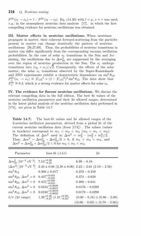
216 14. Neutrino mixing
P 2ν(νl → νx) = 1−P 2ν(νl → νl). Eq. (14.30) with l = µ, x = τ was used,e.g., in the atmospheric neutrino data analysis [17], in which the firstcompelling evidence for neutrino oscillations was obtained.
III. Matter effects in neutrino oscillations. When neutrinospropagate in matter, their coherent forward-scattering from the particlespresent in matter can change drastically the pattern of neutrinooscillations [26,27,69]. Thus, the probabilities of neutrino transitions inmatter can differ significantly from the corresponding vacuum oscillationprobabilities. In the case of solar νe transitions in the Sun and 3-νmixing, the oscillations due to ∆m2
31 are suppressed by the averagingover the region of neutrino production in the Sun. The νe undergotransitions into (νµ + ντ )/
√2. Consequently, the effects of the solar
matter, the solar νe transitions observed by the Super-Kamiokandeand SNO experiments exhibit a characteristic dependence on sin2 θ12:P 3ν⊙ (νe → νe) ∼= |Ue3|4 + (1 − |Ue3|2)2 sin2 θ12. The data show that
P 3ν⊙
∼= 0.3, which is a strong evidence for matter effects for solar νe.
IV. The evidence for flavour neutrino oscillations. We discuss therelevant compelling data in the full edition. The best fit values of theneutrino oscillation parameters and their 3σ allowed ranges, determinedin the latest global analysis of the neutrino oscillation data performed in[174], are given in Table 14.7.
Table 14.7: The best-fit values and 3σ allowed ranges of the3-neutrino oscillation parameters, derived from a global fit of thecurrent neutrino oscillation data (from [174]) . The values (valuesin brackets) correspond to m1 < m2 < m3 (m3 < m1 < m2).The definition of ∆m2 used is: ∆m2 = m2
3 − (m22 + m2
1)/2.Thus, ∆m2 = ∆m2
31 − ∆m221/2 > 0, if m1 < m2 < m3, and
∆m2 = ∆m232 + ∆m2
21/2 < 0 for m3 < m1 < m2.
Parameter best-fit (±1σ) 3σ
∆m221 [10−5 eV 2] 7.54+0.26
−0.22 6.99 − 8.18
|∆m2| [10−3 eV 2] 2.43 ± 0.06 (2.38 ± 0.06) 2.23 − 2.61 (2.19 − 2.56)
sin2 θ12 0.308 ± 0.017 0.259 − 0.359
sin2 θ23, ∆m2 > 0 0.437+0.033−0.023 0.374 − 0.628
sin2 θ23, ∆m2 < 0 0.455+0.039−0.031, 0.380 − 0.641
sin2 θ13, ∆m2 > 0 0.0234+0.0020−0.0019 0.0176− 0.0295
sin2 θ13, ∆m2 < 0 0.0240+0.0019−0.0022 0.0178− 0.0298
δ/π (2σ range) 1.39+0.38−0.27 (1.31+0.29
−0.33) (0.00 − 0.16)⊕ (0.86 − 2.00)
((0.00 − 0.02)⊕ (0.70 − 2.00))
14. Neutrino mixing 217
V. Three neutrino mixing. All compelling data on neutrino oscillationscan be described assuming 3-flavour neutrino mixing in vacuum. In thiscase U can be parametrised as
U =
c12c13 s12c13 s13e−iδ
−s12c23 − c12s23s13eiδ c12c23 − s12s23s13e
iδ s23c13s12s23 − c12c23s13e
iδ −c12s23 − s12c23s13eiδ c23c13
× diag(1, eiα212 , ei
α312 ) . (14.78)
where cij = cos θij , sij = sin θij , the angles θij = [0, π/2], δ = [0, 2π] isthe Dirac CP violation phase and α21, α31 are two Majorana CP violationphases. Global analyses of the neutrino oscillation data [174,175] availableby the second half of 2013 and including, in particular, the latest DayaBay [36], RENO [37] and T2K [151,23] and MINOS [143,147] data,allowed us to determine the 3-neutrino oscillation parameters ∆m2
21, θ12,
|∆m231| (|∆m2
32|), θ23 and θ13 with a relatively high precision.
The existing SK atmospheric neutrino, K2K and MINOS data do notallow to determine the sign of ∆m2
31(32). Maximal solar neutrino mixing,
i.e., θ12 = π/4, is ruled out at more than 6σ by the data. Correspondingly,one has cos 2θ12 ≥ 0.28 (at 99.73% CL).
No experimental information on the CP violation phases in the neutrinomixing matrix U is available. With θ13 6= 0, the Dirac phase δ cangenerate CP violation effects in neutrino oscillations [43,55,56].
The existing data do not allow one to determine the sign of∆m2
A = ∆m231(2). In the case of 3-neutrino mixing, the two possible signs
of ∆m231(2) correspond to two types of neutrino mass spectrum. In the
widely used conventions of numbering the neutrinos with definite mass,the two spectra read: i) Normal Ordering: m1 < m2 < m3, ∆m2
A =
∆m231 > 0, ∆m2
⊙ ≡ ∆m221 > 0, m2(3) = (m2
1 + ∆m221(31))
1
2 ; ii) Inverted
Ordering: m3 < m1 < m2, ∆m2A = ∆m2
32 < 0, ∆m2⊙ ≡ ∆m2
21 > 0,
m2 = (m23 + ∆m2
23)1
2 , m1 = (m23 + ∆m2
23 − ∆m221)
1
2 .
After the spectacular experimental progress made in the studies ofneutrino oscillations, further understanding of the pattern of neutrinomasses and mixing, of their origins and of the status of CP symmetry arethe major goals of the future studies in neutrino physics.
For details and references, see the full Review.
218 15. Quark model
15. QUARK MODEL
Revised August 2013 by C. Amsler (University of Bern), T. DeGrand(University of Colorado, Boulder), and B. Krusche (University of Basel).
15.1. Quantum numbers of the quarks
Quarks are strongly interacting fermions with spin 1/2 and, byconvention, positive parity. Antiquarks have negative parity. Quarks havethe additive baryon number 1/3, antiquarks -1/3. Table 15.1 gives theother additive quantum numbers (flavors) for the three generations ofquarks. They are related to the charge Q (in units of the elementarycharge e) through the generalized Gell-Mann-Nishijima formula
Q = Iz +B + S + C + B + T
2, (15.1)
where B is the baryon number. The convention is that the flavor of aquark (Iz , S, C, B, or T) has the same sign as its charge Q. With thisconvention, any flavor carried by a charged meson has the same sign as itscharge, e.g., the strangeness of the K+ is +1, the bottomness of the B+
is +1, and the charm and strangeness of the D−
s are each −1. Antiquarkshave the opposite flavor signs.
15.2. Mesons
Mesons have baryon number B = 0. In the quark model, they are qq ′
bound states of quarks q and antiquarks q ′ (the flavors of q and q′ maybe different). If the orbital angular momentum of the qq ′ state is ℓ, then
the parity P is (−1)ℓ+1. The meson spin J is given by the usual relation|ℓ − s| ≤ J ≤ |ℓ + s|, where s is 0 (antiparallel quark spins) or 1 (parallel
quark spins). The charge conjugation, or C-parity C = (−1)ℓ+s, is definedonly for the qq states made of quarks and their own antiquarks. TheC-parity can be generalized to the G-parity G = (−1)I+ℓ+s for mesonsmade of quarks and their own antiquarks (isospin Iz = 0), and for thecharged ud and du states (isospin I = 1).
The mesons are classified in JPC multiplets. The ℓ = 0 states are thepseudoscalars (0−+) and the vectors (1−−). The orbital excitations ℓ = 1are the scalars (0++), the axial vectors (1++) and (1+−), and the tensors(2++). Assignments for many of the known mesons are given in Tables15.2 and 15.3. Radial excitations are denoted by the principal quantumnumber n. The very short lifetime of the t quark makes it likely thatbound-state hadrons containing t quarks and/or antiquarks do not exist.
States in the natural spin-parity series P = (−1)J must, according tothe above, have s = 1 and hence, CP = +1. Thus, mesons with naturalspin-parity and CP = −1 (0+−, 1−+, 2+−, 3−+, etc.) are forbidden in
the qq ′ model. The JPC = 0−− state is forbidden as well. Mesons withsuch exotic quantum numbers may exist, but would lie outside the qq ′
model (see section below on exotic mesons).
Following SU(3), the nine possible qq ′ combinations containing thelight u, d, and s quarks are grouped into an octet and a singlet of lightquark mesons:
3 ⊗ 3 = 8⊕ 1 . (15.2)
A fourth quark such as charm c can be included by extending SU(3)to SU(4). However, SU(4) is badly broken owing to the much heavier c
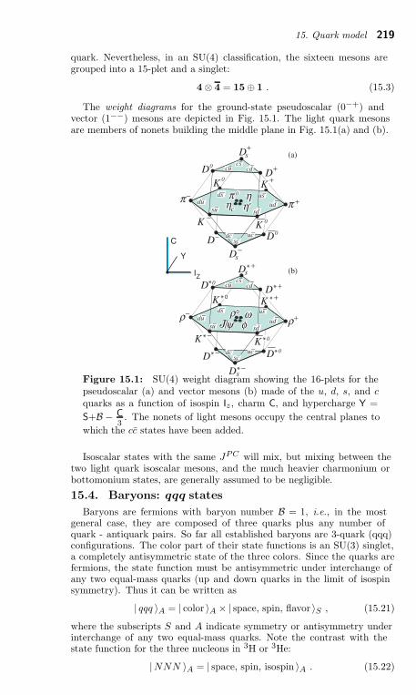
15. Quark model 219
quark. Nevertheless, in an SU(4) classification, the sixteen mesons aregrouped into a 15-plet and a singlet:
4⊗ 4 = 15⊕ 1 . (15.3)
The weight diagrams for the ground-state pseudoscalar (0−+) andvector (1−−) mesons are depicted in Fig. 15.1. The light quark mesonsare members of nonets building the middle plane in Fig. 15.1(a) and (b).
Z
Figure 15.1: SU(4) weight diagram showing the 16-plets for thepseudoscalar (a) and vector mesons (b) made of the u, d, s, and c
quarks as a function of isospin Iz , charm C, and hypercharge Y =
S+B − C3
. The nonets of light mesons occupy the central planes to
which the cc states have been added.
Isoscalar states with the same JPC will mix, but mixing between thetwo light quark isoscalar mesons, and the much heavier charmonium orbottomonium states, are generally assumed to be negligible.
15.4. Baryons: qqq states
Baryons are fermions with baryon number B = 1, i.e., in the mostgeneral case, they are composed of three quarks plus any number ofquark - antiquark pairs. So far all established baryons are 3-quark (qqq)configurations. The color part of their state functions is an SU(3) singlet,a completely antisymmetric state of the three colors. Since the quarks arefermions, the state function must be antisymmetric under interchange ofany two equal-mass quarks (up and down quarks in the limit of isospinsymmetry). Thus it can be written as
| qqq 〉A = | color 〉A × | space, spin, flavor 〉S , (15.21)
where the subscripts S and A indicate symmetry or antisymmetry underinterchange of any two equal-mass quarks. Note the contrast with thestate function for the three nucleons in 3H or 3He:
|NNN 〉A = | space, spin, isospin 〉A . (15.22)
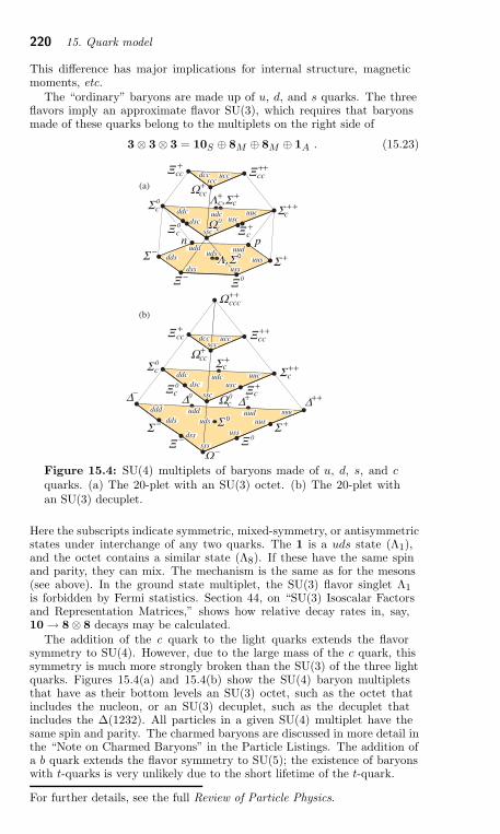
220 15. Quark model
This difference has major implications for internal structure, magneticmoments, etc.
The “ordinary” baryons are made up of u, d, and s quarks. The threeflavors imply an approximate flavor SU(3), which requires that baryonsmade of these quarks belong to the multiplets on the right side of
3⊗ 3⊗ 3 = 10S ⊕ 8M ⊕ 8M ⊕ 1A . (15.23)
Figure 15.4: SU(4) multiplets of baryons made of u, d, s, and c
quarks. (a) The 20-plet with an SU(3) octet. (b) The 20-plet withan SU(3) decuplet.
Here the subscripts indicate symmetric, mixed-symmetry, or antisymmetricstates under interchange of any two quarks. The 1 is a uds state (Λ1),and the octet contains a similar state (Λ8). If these have the same spinand parity, they can mix. The mechanism is the same as for the mesons(see above). In the ground state multiplet, the SU(3) flavor singlet Λ1
is forbidden by Fermi statistics. Section 44, on “SU(3) Isoscalar Factorsand Representation Matrices,” shows how relative decay rates in, say,10 → 8⊗ 8 decays may be calculated.
The addition of the c quark to the light quarks extends the flavorsymmetry to SU(4). However, due to the large mass of the c quark, thissymmetry is much more strongly broken than the SU(3) of the three lightquarks. Figures 15.4(a) and 15.4(b) show the SU(4) baryon multipletsthat have as their bottom levels an SU(3) octet, such as the octet thatincludes the nucleon, or an SU(3) decuplet, such as the decuplet thatincludes the ∆(1232). All particles in a given SU(4) multiplet have thesame spin and parity. The charmed baryons are discussed in more detail inthe “Note on Charmed Baryons” in the Particle Listings. The addition ofa b quark extends the flavor symmetry to SU(5); the existence of baryonswith t-quarks is very unlikely due to the short lifetime of the t-quark.
For further details, see the full Review of Particle Physics.
16. Grand Unified Theories 221
16. GRAND UNIFIED THEORIES
Updated October 2011 by S. Raby (Ohio State University).
In spite of all the successes of the Standard Model [SM] it is unlikelyto be the final theory. It leaves many unanswered questions. Why thelocal gauge interactions SU(3)C × SU(2)L × U(1)Y and why 3 familiesof quarks and leptons? Moreover why does one family consist of thestates [Q, uc, dc; L, ec] transforming as [(3, 2, 1/3), (3, 1,−4/3), (3, 1, 2/3);(1, 2,−1), (1, 1, 2)], where Q = (u, d) and L = (ν, e) are SU(2)L doubletsand uc, dc, ec are charge conjugate SU(2)L singlet fields with the U(1)Yquantum numbers given? [We use the convention that electric chargeQEM = T3L + Y/2 and all fields are left handed.] Note the SM gaugeinteractions of quarks and leptons are completely fixed by their gaugecharges. Thus, if we understood the origin of this charge quantization,we would also understand why there are no fractionally charged hadrons.Finally, what is the origin of quark and lepton masses; the family masshierarchy and quark mixing angles? Perhaps if we understood this, wewould also understand neutrino masses, the origin of CP violation, thecosmological matter - antimatter asymmetry or even the nature of darkmatter.
In the Standard Model, quarks and leptons are on an equal footing;both fundamental particles without substructure. It is now clear that theymay be two faces of the same coin; unified, for example, by extending QCD(or SU(3)C) to include leptons as the fourth color, SU(4)C . The completePati-Salam gauge group is SU(4)C × SU(2)L × SU(2)R with the statesof one family [(Q, L), (Qc, Lc)] transforming as [(4, 2, 1), (4, 1, 2)] whereQc = (dc, uc), Lc = (ec, νc) are doublets under SU(2)R. Electric charge isnow given by the relation QEM = T3L + T3R + 1/2(B − L) and SU(4)Ccontains the subgroup SU(3)C × (B − L) where B (L) is baryon (lepton)number. Note νc has no SM quantum numbers and is thus completely“sterile.” It is introduced to complete the SU(2)R lepton doublet. Thisadditional state is desirable when considering neutrino masses.
Although quarks and leptons are unified with the states of one familyforming two irreducible representations of the gauge group; there arestill 3 independent gauge couplings (two if one also imposes parity, i.e.
L ↔ R symmetry). As a result the three low energy gauge couplingsare still independent arbitrary parameters. This difficulty is resolved byembedding the SM gauge group into the simple unified gauge group,Georgi-Glashow SU(5), with one universal gauge coupling αG definedat the grand unification scale MG. Quarks and leptons still sit intwo irreducible representations, as before, with a 10 = [Q, uc, ec] and5 = [dc, L]. Nevertheless, the three low energy gauge couplings are nowdetermined in terms of two independent parameters : αG and MG. Hence,there is one prediction.
In order to break the electroweak symmetry at the weak scale and givemass to quarks and leptons, Higgs doublets are needed which can sit ineither a 5H or 5H. The additional 3 states are color triplet Higgs scalars.The couplings of these color triplets violate baryon and lepton numberand nucleons decay via the exchange of a single color triplet Higgs scalar.Hence, in order not to violently disagree with the non-observation ofnucleon decay, their mass must be greater than ∼ 1010−11 GeV. Note, insupersymmetric GUTs, in order to cancel anomalies as well as give massto both up and down quarks, both Higgs multiplets 5H, 5H are required.
222 16. Grand Unified Theories
As we shall discuss later, nucleon decay now constrains the color tripletHiggs states in a SUSY GUT to have mass significantly greater than MG.
Complete unification is possible with the symmetry group SO(10) withone universal gauge coupling αG and one family of quarks and leptonssitting in the 16 dimensional spinor representation 16 = [10 + 5 + 1].The SU(5) singlet 1 is identified with νc. SO(10) has two inequivalentmaximal breaking patterns. SO(10) → SU(5) × U(1)X and SO(10) →SU(4)C × SU(2)L × SU(2)R. In the first case we obtain Georgi-GlashowSU(5) if QEM is given in terms of SU(5) generators alone or so-calledflipped SU(5) if QEM is partly in U(1)X . In the latter case we havethe Pati-Salam symmetry. If SO(10) breaks directly to the SM at MG,then we retain the prediction for gauge coupling unification. Howevermore possibilities for breaking (hence, more breaking scales and moreparameters) are available in SO(10). Nevertheless, with one breakingpattern SO(10) → SU(5) → SM, where the last breaking scale is MG,the predictions from gauge coupling unification are preserved. TheHiggs multiplets in minimal SO(10) are contained in the fundamental10H = [5H, 5H] representation. Note only in SO(10) does the gaugesymmetry distinguish quark and lepton multiplets from Higgs multiplets.Finally, larger symmetry groups have been considered, e.g. E(6), SU(6),etc. They however always include extra, unwanted states; making theselarger symmetry groups unattractive starting points for model building.
Let us now consider the primary GUT prediction, i.e gauge couplingunification. The GUT symmetry is spontaneously broken at the scaleMG and all particles not in the SM obtain mass of order MG. Whencalculating Green’s functions with external energies E ≫ MG, we canneglect the mass of all particles in the loop and hence, all particlescontribute to the renormalization group running of the universal gaugecoupling. However, for E ≪ MG one can consider an effective field theory(EFT) including only the states with mass < E ≪ MG. The gaugesymmetry of the EFT [valid below MG] is SU(3)C × SU(2)L × U(1)Yand the three gauge couplings renormalize independently. The statesof the EFT include only those of the SM; 12 gauge bosons, 3 familiesof quarks and leptons and one or more Higgs doublets. At MG thetwo effective theories [the GUT itself is most likely the EFT of amore fundamental theory defined at a higher scale] must give identicalresults; hence we have the boundary conditions g3 = g2 = g1 ≡ gGwhere at any scale µ < MG we have g2 ≡ g and g1 =
√
5/3 g′.[Note, the hypercharge coupling is rescaled in order for Y to satisfy thecharge quantization of the GUT. Also αs = (g2
3/4π), αEM = (e2/4π)
(e = g sin θW ) and sin2 θW = (g′)2/(g2 + (g′)2).] Then using two lowenergy couplings, such as αs(MZ), αEM (MZ), the two independentparameters αG, MG can be fixed. The third gauge coupling, sin2 θW inthis case, is then predicted. This was the procedure up until about 1991.Subsequently, the uncertainties in sin2 θW were reduced ten fold. Sincethen, αEM (MZ), sin2 θW have been used as input to predict αG, MG andαs(MZ).
Note, the above boundary condition is only valid when using oneloop renormalization group [RG] running. With precision electroweakdata, however, it is necessary to use two loop RG running. Hence,one must include one loop threshold corrections to gauge couplingboundary conditions at both the weak and GUT scales. In this caseit is always possible to define the GUT scale as the point where
16. Grand Unified Theories 223
α1(MG) = α2(MG) ≡ αG and α3(MG) = αG (1 + ǫ3). The thresholdcorrection ǫ3 is a logarithmic function of all states with mass of order MGand αG = αG + ∆ where αG is the GUT coupling constant above MG and∆ is a one loop threshold correction. To the extent that gauge couplingunification is perturbative, the GUT threshold corrections are small andcalculable. This presumes that the GUT scale is sufficiently below thePlanck scale or any other strong coupling extension of the GUT, such as astrongly coupled string theory.
Supersymmetric grand unified theories [SUSY GUTs] are an extensionof non-SUSY GUTs. The key difference between SUSY GUTs and non-SUSY GUTs is the low energy effective theory which, in a SUSY GUT,also satisfies N=1 supersymmetry down to scales of order the weak scale.Hence, the spectrum includes all the SM states plus their supersymmetricpartners. It also includes one pair (or more) of Higgs doublets; one to givemass to up-type quarks and the other to down-type quarks and chargedleptons. Two doublets with opposite hypercharge Y are also needed tocancel fermionic triangle anomalies. Note, a low energy SUSY breakingscale (the scale at which the SUSY partners of SM particles obtain mass)is necessary to solve the gauge hierarchy problem.
Simple non-SUSY SU(5) is ruled out; initially by the increased accuracyin the measurement of sin2 θW and by early bounds on the proton lifetime(see below). However, by now LEP data has conclusively shown thatSUSY GUTs is the new standard model; by which we mean the theoryused to guide the search for new physics beyond the present SM. SUSYextensions of the SM have the property that their effects decouple as theeffective SUSY breaking scale is increased. Any theory beyond the SMmust have this property simply because the SM works so well. However,the SUSY breaking scale cannot be increased with impunity, since thiswould reintroduce a gauge hierarchy problem. Unfortunately there isno clear-cut answer to the question, when is the SUSY breaking scaletoo high. A conservative bound would suggest that the third generationquarks and leptons must be lighter than about 1 TeV, in order that theone loop corrections to the Higgs mass from Yukawa interactions remainsof order the Higgs mass bound itself.
At present gauge coupling unification within SUSY GUTs worksextremely well. Exact unification at MG, with two loop renormalizationgroup running from MG to MZ , and one loop threshold corrections at theweak scale, fits to within 3 σ of the present precise low energy data. Asmall threshold correction at MG (ǫ3 ∼ −4%) is sufficient to fit the lowenergy data precisely.* This may be compared to non-SUSY GUTs wherethe fit misses by ∼ 12 σ and a precise fit requires new weak scale states inincomplete GUT multiplets or multiple GUT breaking scales.
Baryon number is necessarily violated in any GUT. In SU(5) nucleonsdecay via the exchange of gauge bosons with GUT scale masses, resultingin dimension 6 baryon number violating operators suppressed by (1/M2
G).
The nucleon lifetime is calculable and given by τN ∝ M4G/(α2
G m5p). The
* This result implicitly assumes universal GUT boundary conditions forsoft SUSY breaking parameters at MG. In the simplest case we have auniversal gaugino mass M1/2, a universal mass for squarks and sleptons
m16 and a universal Higgs mass m10, as motivated by SO(10). In somecases, threshold corrections to gauge coupling unification can be exchangedfor threshold corrections to soft SUSY parameters.
224 16. Grand Unified Theories
dominant decay mode of the proton (and the baryon violating decay modeof the neutron), via gauge exchange, is p → e+ π0 (n → e+ π−). Inany simple gauge symmetry, with one universal GUT coupling and scale(αG, MG), the nucleon lifetime from gauge exchange is calculable. Hence,the GUT scale may be directly observed via the extremely rare decayof the nucleon. Experimental searches for nucleon decay began with theKolar Gold Mine, Homestake, Soudan, NUSEX, Frejus, HPW, and IMBdetectors. The present experimental bounds come from Super-Kamiokandeand Soudan II. We discuss these results shortly. Non-SUSY GUTs arealso ruled out by the non-observation of nucleon decay. In SUSY GUTs,the GUT scale is of order 3 × 10¹⁶ GeV, as compared to the GUT scalein non-SUSY GUTs which is of order 1015 GeV. Hence, the dimension6 baryon violating operators are significantly suppressed in SUSY GUTswith τp ∼ 1034−38 yrs.
However, in SUSY GUTs there are additional sources for baryonnumber violation – dimension 4 and 5 operators. Although the notationdoes not change, when discussing SUSY GUTs all fields are implicitlybosonic superfields and the operators considered are the so-called Fterms which contain two fermionic components and the rest scalars orproducts of scalars. Within the context of SU(5) the dimension 4 and5 operators have the form (10 5 5) ⊃ (uc dc dc) + (Q L dc) + (ec L L)and (10 10 10 5) ⊃ (Q Q Q L) + (uc uc dc ec) + B and L conservingterms, respectively. The dimension 4 operators are renormalizable withdimensionless couplings; similar to Yukawa couplings. On the other hand,the dimension 5 operators have a dimensionful coupling of order (1/MG).
The dimension 4 operators violate baryon number or lepton number,respectively, but not both. The nucleon lifetime is extremely short ifboth types of dimension 4 operators are present in the low energy theory.However both types can be eliminated by requiring R parity. In SU(5) theHiggs doublets reside in a 5H, 5H and R parity distinguishes the 5 (quarksand leptons) from 5H (Higgs). R parity (or its cousin, family reflectionsymmetry takes F → −F, H → H with F = 10, 5, H = 5H, 5H.This forbids the dimension 4 operator (10 5 5), but allows the Yukawacouplings of the form (10 5 5H) and (10 10 5H). It also forbids thedimension 3, lepton number violating, operator (5 5H) ⊃ (L Hu) with acoefficient with dimensions of mass which, like the µ parameter, could beof order the weak scale and the dimension 5, baryon number violating,operator (10 10 10 5H) ⊃ (Q Q Q Hd) + · · ·. Note, R parity is theonly known symmetry [consistent with a SUSY GUT] which can preventunwanted dimension four operators. Hence, by naturalness arguments,R parity must be a symmetry in the effective low energy theory of anySUSY GUT. This does not mean to say that R parity is guaranteed to besatisfied in any GUT.
Dimension 5 baryon number violating operators are genericallygenerated via color triplet Higgsino exchange. Hence, the color tripletpartners of Higgs doublets must necessarily obtain mass of order theGUT scale. The dominant decay modes from dimension 5 operatorsare p → K+ ν (n → K0 ν). Note, final states with a second or thirdgeneration particle are dominant. This is due to a simple symmetryargument. The operators (Qi Qj Qk Ll), (uc
i ucj dc
k ecl ) (where
i, j, k, l = 1, 2, 3 are family indices and color and weak indices areimplicit) must be invariant under SU(3)C and SU(2)L. Hence, their colorand weak doublet indices must be anti-symmetrized. However this product
16. Grand Unified Theories 225
of bosonic superfields must be totally symmetric under interchange of allindices. Thus, the first operator vanishes for i = j = k and the secondvanishes for i = j.
Recent Super-Kamiokande bounds on the proton lifetime severelyconstrain these dimension 6 and 5 operators with (172.8 kt-yr) of datathey find τ(p→e+π0) > 1.0 × 1034 yrs, τ(p→K+ν) > 3.3 × 1033 yrs and
τ(n→e+π−) > 2 × 1033 yrs at (90% CL). These constraints are now
sufficient to rule out minimal SUSY SU(5). However non-minimal Higgssectors in SU(5) or minimal SO(10) theories still survive. The upperbound on the proton lifetime from these theories are approximately afactor of 5 above the experimental bounds. Hence, if SUSY GUTs arecorrect, nucleon decay must be seen soon.
Is there a way out of this conclusion? String theories, and recentfield theoretic constructions, contain grand unified symmetries realized inhigher dimensions. Upon compactification to four dimensions, the GUTsymmetry is typically broken directly to the MSSM. A positive feature ofthis approach is that the color triplet Higgs states are projected out ofthe low energy spectrum. At the same time, quark and lepton states nowemanate from different GUT multiplets. As a consequence, proton decaydue to dimension 5 and 6 operators can be severely suppressed, eliminatedall together or sometimes even enhanced. Hence, the observation of protondecay may distinguish extra-dimensional GUTs from four dimensionalones. For example, a simple ZR
4 symmetry, consistent with SO(10), withR parity as a subgroup can also forbid the mu term and dimension 5 Band L violating operators to all orders in perturbation theory. They maythen be generated, albeit sufficiently suppressed, via non-perturbativeeffects. In this case, proton decay is completely dominated by dimension 6operators.
Grand unification of the strong and electroweak interactions at aunique high energy scale MG ∼ 3 × 10¹⁶ GeV requires [1] gauge couplingunification, [2] low energy supersymmetry [with a large SUSY desert], and[3] nucleon decay. The first prediction has already been verified. Perhapsthe next two will be seen soon. Whether or not Yukawa couplings unify ismore model dependent. Nevertheless, the 16 dimensional representationof quarks and leptons in SO(10) is very compelling and may yet leadto an understanding of fermion masses and mixing angles. GUTs alsomake predictions for Yukawa coupling unification, they provide a naturalframework for neutrino masses and mixing angles, magnetic monopoles,baryogenesis, etc. For a more comprehensive discussion of GUTs, see theunabridged particle data book. In any event, the experimental verificationof the first three pillars of SUSY GUTs would forever change our viewof Nature. Moreover, the concomitant evidence for a vast SUSY desertwould expose a huge lever arm for discovery. For then it would becomeclear that experiments probing the TeV scale could reveal physics at theGUT scale and perhaps beyond.
Further discussion and references may be found in the full Review .
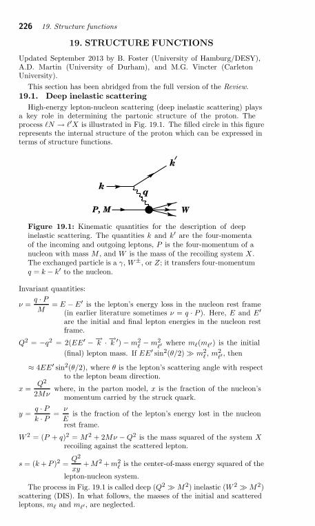
226 19. Structure functions
19. STRUCTURE FUNCTIONS
Updated September 2013 by B. Foster (University of Hamburg/DESY),A.D. Martin (University of Durham), and M.G. Vincter (CarletonUniversity).
This section has been abridged from the full version of the Review.
19.1. Deep inelastic scattering
High-energy lepton-nucleon scattering (deep inelastic scattering) playsa key role in determining the partonic structure of the proton. Theprocess ℓN → ℓ′X is illustrated in Fig. 19.1. The filled circle in this figurerepresents the internal structure of the proton which can be expressed interms of structure functions.
k
k
q
P, M W
Figure 19.1: Kinematic quantities for the description of deepinelastic scattering. The quantities k and k′ are the four-momentaof the incoming and outgoing leptons, P is the four-momentum of anucleon with mass M , and W is the mass of the recoiling system X .The exchanged particle is a γ, W±, or Z; it transfers four-momentumq = k − k′ to the nucleon.
Invariant quantities:
ν =q · PM
= E − E′ is the lepton’s energy loss in the nucleon rest frame(in earlier literature sometimes ν = q · P ). Here, E and E′
are the initial and final lepton energies in the nucleon restframe.
Q2 = −q2 = 2(EE′ − −→k · −→k ′) − m2
ℓ − m2ℓ′
where mℓ(mℓ′) is the initial
(final) lepton mass. If EE′ sin2(θ/2) ≫ m2ℓ , m2
ℓ′, then
≈ 4EE′ sin2(θ/2), where θ is the lepton’s scattering angle with respectto the lepton beam direction.
x =Q2
2Mνwhere, in the parton model, x is the fraction of the nucleon’s
momentum carried by the struck quark.
y =q · Pk · P =
ν
Eis the fraction of the lepton’s energy lost in the nucleon
rest frame.
W 2 = (P + q)2 = M2 + 2Mν − Q2 is the mass squared of the system Xrecoiling against the scattered lepton.
s = (k + P )2 =Q2
xy+ M2 + m2
ℓ is the center-of-mass energy squared of the
lepton-nucleon system.
The process in Fig. 19.1 is called deep (Q2 ≫ M2) inelastic (W 2 ≫ M2)scattering (DIS). In what follows, the masses of the initial and scatteredleptons, mℓ and mℓ′ , are neglected.
19. Structure functions 227
19.1.1. DIS cross sections :d2σ
dx dy= x (s − M2)
d2σ
dx dQ2=
2π Mν
E′
d2σ
dΩNrest dE′. (19.1)
In lowest-order perturbation theory, the cross section for the scattering ofpolarized leptons on polarized nucleons can be expressed in terms of theproducts of leptonic and hadronic tensors associated with the coupling ofthe exchanged bosons at the upper and lower vertices in Fig. 19.1 (seeRefs. 1–4)
d2σ
dxdy=
2πyα2
Q4
∑
j
ηj Lµνj W j
µν . (19.2)
For neutral-current processes, the summation is over j = γ, Z and γZrepresenting photon and Z exchange and the interference between them,whereas for charged-current interactions there is only W exchange,j = W . (For transverse nucleon polarization, there is a dependence onthe azimuthal angle of the scattered lepton.) The lepton tensor Lµν isassociated with the coupling of the exchange boson to the leptons. Forincoming leptons of charge e = ±1 and helicity λ = ±1,
Lγµν = 2
(
kµk′ν + k′µkν − (k · k′ − m2ℓ )gµν − iλεµναβkαk′β
)
,
LγZµν =(ge
V + eλgeA) Lγ
µν , LZµν = (ge
V + eλgeA)2 Lγ
µν ,
LWµν =(1 + eλ)2 Lγ
µν , (19.3)
where geV = − 1
2+ 2 sin2 θW , ge
A = − 1
2.
Although here the helicity formalism is adopted, an alternative approachis to express the tensors in Eq. (19.3) in terms of the polarization of thelepton.
The factors ηj in Eq. (19.2) denote the ratios of the correspondingpropagators and couplings to the photon propagator and coupling squared
ηγ = 1 ; ηγZ =
(
GF M2Z
2√
2πα
) (
Q2
Q2 + M2Z
)
;
ηZ = η2γZ ; ηW = 1
2
(
GF M2W
4πα
Q2
Q2 + M2W
)2
. (19.4)
The hadronic tensor, which describes the interaction of the appropriateelectroweak currents with the target nucleon, is given by
Wµν =1
4π
∫
d4z eiq·z⟨
P, S∣
∣
∣
[
J†µ(z), Jν(0)
]∣
∣
∣P, S
⟩
, (19.5)
where S denotes the nucleon-spin 4-vector, with S2 = −M2 and S ·P = 0.
19.2. Structure functions of the proton
The structure functions are defined in terms of the hadronic tensor (seeRefs. 1–3)
Wµν =
(
−gµν +qµqν
q2
)
F1(x, Q2) +PµPν
P · q F2(x, Q2)
− iεµναβqαPβ
2P · q F3(x, Q2)
+ iεµναβqα
P · q
[
Sβg1(x, Q2) +
(
Sβ − S · qP · q Pβ
)
g2(x, Q2)
]
228 19. Structure functions
+1
P · q
[
1
2
(
PµSν + SµPν
)
− S · qP · q PµPν
]
g3(x, Q2)
+S · qP · q
[
PµPν
P · q g4(x, Q2) +
(
−gµν +qµqν
q2
)
g5(x, Q2)
]
(19.6)
where
Pµ = Pµ − P · qq2
qµ, Sµ = Sµ − S · qq2
qµ . (19.7)
The cross sections for neutral- and charged-current deep inelasticscattering on unpolarized nucleons can be written in terms of the structurefunctions in the generic form
d2σi
dxdy=
4πα2
xyQ2ηi
(
1 − y − x2y2M2
Q2
)
F i2
+ y2xF i1 ∓
(
y − y2
2
)
xF i3
, (19.8)
where i = NC, CC corresponds to neutral-current (eN → eX) or charged-current (eN → νX or νN → eX) processes, respectively. For incoming
neutrinos, LWµν of Eq. (19.3) is still true, but with e, λ corresponding to
the outgoing charged lepton. In the last term of Eq. (19.8), the − sign istaken for an incoming e+ or ν and the + sign for an incoming e− or ν.The factor ηNC = 1 for unpolarized e± beams, whereas
ηCC = (1 ± λ)2ηW (19.9)
with ± for ℓ±; and where λ is the helicity of the incoming lepton andηW is defined in Eq. (19.4); for incoming neutrinos ηCC = 4ηW . The CCstructure functions, which derive exclusively from W exchange, are
FCC1 = FW
1 , FCC2 = FW
2 , xFCC3 = xFW
3 . (19.10)
The NC structure functions Fγ2
, FγZ2
, FZ2 are, for e±N → e±X , given by
Ref. 5,
FNC2 = F γ
2− (ge
V ±λgeA)ηγZF γZ
2+ (ge 2
V +ge 2A ±2λge
V geA) ηZFZ
2 (19.11)
and similarly for FNC1 , whereas
xFNC3 = −(ge
A±λgeV )ηγZxF
γZ3
+[2geV ge
A±λ(ge 2V +ge 2
A )]ηZxFZ3 . (19.12)
The polarized cross-section difference
∆σ = σ(λn = −1, λℓ) − σ(λn = 1, λℓ) , (19.13)
where λℓ, λn are the helicities (±1) of the incoming lepton and nucleon,respectively, may be expressed in terms of the five structure functionsg1,...5(x, Q2) of Eq. (19.6). Thus,
d2∆σi
dxdy=
8πα2
xyQ2ηi
−λℓy
(
2 − y − 2x2y2 M2
Q2
)
xgi1 + λℓ4x3y2 M2
Q2gi2
+ 2x2yM2
Q2
(
1 − y − x2y2 M2
Q2
)
gi3
−(
1 + 2x2yM2
Q2
) [(
1 − y − x2y2 M2
Q2
)
gi4 + xy2gi
5
]
(19.14)
19. Structure functions 229
with i = NC or CC as before. In the M2/Q2 → 0 limit, Eq. (19.8) andEq. (19.14) may be written in the form
d2σi
dxdy=
2πα2
xyQ2ηi
[
Y+F i2 ∓ Y−xF i
3 − y2F iL
]
,
d2∆σi
dxdy=
4πα2
xyQ2ηi
[
−Y+gi4 ∓ Y−2xgi
1 + y2giL
]
, (19.16)
with i = NC or CC, where Y± = 1 ± (1 − y)2 and
F iL = F i
2 − 2xF i1 , gi
L = gi4 − 2xgi
5 . (19.17)
In the naive quark-parton model, the analogy with the Callan-Grossrelations [6] F i
L = 0, are the Dicus relations [7] giL = 0. Therefore,
there are only two independent polarized structure functions: g1 (parityconserving) and g5 (parity violating), in analogy with the unpolarizedstructure functions F1 and F3.
19.2.1. Structure functions in the quark-parton model :
In the quark-parton model [8,9], contributions to the structurefunctions F i and gi can be expressed in terms of the quark distributionfunctions q(x, Q2) of the proton, where q = u, u, d, d etc.The quantityq(x, Q2)dx is the number of quarks (or antiquarks) of designated flavorthat carry a momentum fraction between x and x + dx of the proton’smomentum in a frame in which the proton momentum is large.
For the neutral-current processes ep → eX ,[
F γ2
, F γZ2
, FZ2
]
= x∑
q
[
e2q , 2eqg
qV
, gq 2
V+ gq 2
A
]
(q + q) ,
[
Fγ3
, FγZ3
, FZ3
]
=∑
q
[
0, 2eqgqA, 2g
qV g
qA
]
(q − q) ,
[
gγ1, gγZ
1, gZ
1
]
= 1
2
∑
q
[
e2q , 2eqg
qV , gq 2
V + gq 2
A
]
(∆q + ∆q) ,
[
gγ5, g
γZ5
, gZ5
]
=∑
q
[
0, eqgqA, g
qV g
qA
]
(∆q − ∆q) , (19.18)
where gqV = ± 1
2− 2eq sin2 θW and g
qA = ± 1
2, with ± according to whether
q is a u− or d−type quark respectively. The quantity ∆q is the differenceq ↑ −q ↓ of the distributions with the quark spin parallel and antiparallelto the proton spin.
For the charged-current processes e−p → νX and νp → e+X , thestructure functions are:
FW−
2 = 2x(u + d + s + c . . .) , FW−
3 = 2(u − d − s + c . . .) , (19.19)
gW−
1 = (∆u + ∆d + ∆s + ∆c . . .) , gW−
5 = (−∆u + ∆d + ∆s − ∆c . . .) ,
where only the active flavors are to be kept and where CKM mixing hasbeen neglected. For e+p → νX and νp → e−X , the structure functions
FW+, gW+
are obtained by the flavor interchanges d ↔ u, s ↔ c in the
expressions for FW−
, gW−
. The structure functions for scattering on aneutron are obtained from those of the proton by the interchange u ↔ d.For both the neutral- and charged-current processes, the quark-partonmodel predicts 2xF i
1 = F i2 and gi
4 = 2xgi5.
Further discussion may be found in the full Review of Particle Physics .
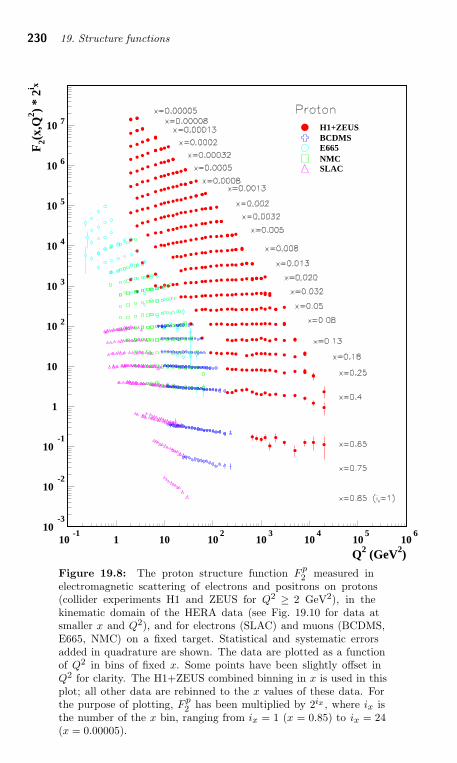
230 19. Structure functions
Q2 (GeV2)
F2(
x,Q
2 ) *
2i x
H1+ZEUSBCDMSE665NMCSLAC
10-3
10-2
10-1
1
10
10 2
10 3
10 4
10 5
10 6
10 7
10-1
1 10 102
103
104
105
106
Figure 19.8: The proton structure function Fp2
measured inelectromagnetic scattering of electrons and positrons on protons(collider experiments H1 and ZEUS for Q2 ≥ 2 GeV2), in thekinematic domain of the HERA data (see Fig. 19.10 for data atsmaller x and Q2), and for electrons (SLAC) and muons (BCDMS,E665, NMC) on a fixed target. Statistical and systematic errorsadded in quadrature are shown. The data are plotted as a functionof Q2 in bins of fixed x. Some points have been slightly offset inQ2 for clarity. The H1+ZEUS combined binning in x is used in thisplot; all other data are rebinned to the x values of these data. Forthe purpose of plotting, F
p2
has been multiplied by 2ix , where ix isthe number of the x bin, ranging from ix = 1 (x = 0.85) to ix = 24(x = 0.00005).
22. Big-Bang cosmology 231
22. BIG-BANG COSMOLOGY
Revised September 2013 by K.A. Olive (University of Minnesota) andJ.A. Peacock (University of Edinburgh).
22.1. Introduction to Standard Big-Bang Model
The observed expansion of the Universe [1–3] is a natural (almostinevitable) result of any homogeneous and isotropic cosmological modelbased on general relativity. In order to account for the possibility that theabundances of the elements had a cosmological origin, Alpher and Hermanproposed that the early Universe which was once very hot and dense(enough so as to allow for the nucleosynthetic processing of hydrogen),and has expanded and cooled to its present state [4,5]. In 1948, Alpherand Herman predicted that a direct consequence of this model is thepresence of a relic background radiation with a temperature of order afew K [6,7]. It was the observation of the 3 K background radiation thatsingled out the Big-Bang model as the prime candidate to describe ourUniverse. Subsequent work on Big-Bang nucleosynthesis further confirmedthe necessity of our hot and dense past. These relativistic cosmologicalmodels face severe problems with their initial conditions, to which the bestmodern solution is inflationary cosmology.
22.1.1. The Robertson-Walker Universe :The observed homogeneity and isotropy enable us to describe the overall
geometry and evolution of the Universe in terms of two cosmologicalparameters accounting for the spatial curvature and the overall expansion(or contraction) of the Universe. These two quantities appear in the mostgeneral expression for a space-time metric which has a (3D) maximallysymmetric subspace of a 4D space-time, known as the Robertson-Walkermetric:
ds2 = dt2 − R2(t)
[
dr2
1 − kr2+ r2 (dθ2 + sin2 θ dφ2)
]
. (22.1)
Note that we adopt c = 1 throughout. By rescaling the radial coordinate,we can choose the curvature constant k to take only the discrete values+1, −1, or 0 corresponding to closed, open, or spatially flat geometries.
22.1.2. The redshift :The cosmological redshift is a direct consequence of the Hubble
expansion, determined by R(t). A local observer detecting light from adistant emitter sees a redshift in frequency. We can define the redshift as
z ≡ ν1 − ν2
ν2≃ v12 , (22.3)
where ν1 is the frequency of the emitted light, ν2 is the observed frequencyand v12 is the relative velocity between the emitter and the observer.While the definition, z = (ν1 − ν2)/ν2 is valid on all distance scales,relating the redshift to the relative velocity in this simple way is only trueon small scales (i.e., less than cosmological scales) such that the expansionvelocity is non-relativistic. For light signals, we can use the metric givenby Eq. (22.1) and ds2 = 0 to write
1 + z =ν1
ν2=
R2
R1. (22.5)
This result does not depend on the non-relativistic approximation.
22.1.3. The Friedmann-Lemaıtre equations of motion :The cosmological equations of motion are derived from Einstein’s
equationsRµν − 1
2gµνR = 8πGNTµν + Λgµν . (22.6)
232 22. Big-Bang cosmology
Gliner [17] and Zeldovich [18] have pioneered the modern view, inwhich the Λ term is taken to the rhs and interpreted as an effectiveenergy–momentum tensor Tµν for the vacuum of Λgµν/8πGN. It iscommon to assume that the matter content of the Universe is a perfectfluid, for which
Tµν = −pgµν + (p + ρ)uµuν , (22.7)
where gµν is the space-time metric described by Eq. (22.1), p is theisotropic pressure, ρ is the energy density and u = (1, 0, 0, 0) is thevelocity vector for the isotropic fluid in co-moving coordinates. With theperfect fluid source, Einstein’s equations lead to the Friedmann-Lemaıtreequations
H2 ≡(
R
R
)2
=8π GN ρ
3− k
R2+
Λ
3, (22.8)
and R
R=
Λ
3− 4πGN
3(ρ + 3p) , (22.9)
where H(t) is the Hubble parameter and Λ is the cosmological constant.The first of these is sometimes called the Friedmann equation. Energyconservation via T
µν;µ = 0, leads to a third useful equation
ρ = −3H (ρ + p) . (22.10)Eq. (22.10) can also be simply derived as a consequence of the first lawof thermodynamics. For Λ = 0, it is clear that the Universe must beexpanding or contracting.
22.1.4. Definition of cosmological parameters :The Friedmann equation can be used to define a critical density such
that k = 0 when Λ = 0,
ρc ≡ 3H2
8π GN
= 1.88 × 10⁻²⁶ h2 kg m−3
= 1.05 × 10⁻⁵ h2 GeV cm−3 ,
(22.11)
where the scaled Hubble parameter, h, is defined by
H ≡ 100 h km s−1 Mpc−1
⇒ H−1 = 9.78 h−1 Gyr
= 2998 h−1 Mpcρc .
(22.12)
The cosmological density parameter Ωtot is defined as the energy densityrelative to the critical density,
Ωtot = ρ/ρc . (22.13)Note that one can now rewrite the Friedmann equation as
k/R2 = H2(Ωtot − 1) . (22.14)
From Eq. (22.14), one can see that when Ωtot > 1, k = +1 and theUniverse is closed, when Ωtot < 1, k = −1 and the Universe is open, andwhen Ωtot = 1, k = 0, and the Universe is spatially flat.
It is often necessary to distinguish different contributions to thedensity. It is therefore convenient to define present-day density parametersfor pressureless matter (Ωm) and relativistic particles (Ωr), plus thequantity ΩΛ = Λ/3H2. In more general models, we may wish to drop theassumption that the vacuum energy density is constant, and we thereforedenote the present-day density parameter of the vacuum by Ωv. TheFriedmann equation then becomes
k/R20 = H2
0 (Ωm + Ωr + Ωv − 1) , (22.15)
22. Big-Bang cosmology 233
where the subscript 0 indicates present-day values. Thus, it is the sum ofthe densities in matter, relativistic particles, and vacuum that determinesthe overall sign of the curvature. Note that the quantity −k/R2
0H20 is
sometimes (unfortunately) referred to as Ωk.
22.1.5. Standard Model solutions :During inflation and again today the expansion rate for the Universe
is accelerating, and domination by a cosmological constant or some otherform of dark energy should be considered.
Let us first assume a general equation of state parameter for a singlecomponent, w = p/ρ which is constant. In this case, Eq. (22.10) can be
written as ρ = −3(1 + w)ρR/R and is easily integrated to yield
ρ ∝ R−3(1+w) . (22.16)Note that at early times when R is small, k/R2 in the Friedmann equationcan be neglected so long as w > −1/3. Curvature domination occurs atrather late times (if a cosmological constant term does not dominatesooner). For w 6= −1,
R(t) ∝ t2/[3(1+w)] . (22.17)
22.1.5.2. A Radiation-dominated Universe:
In the early hot and dense Universe, it is appropriate to assume anequation of state corresponding to a gas of radiation (or relativisticparticles) for which w = 1/3. In this case, Eq. (22.16) becomes ρ ∝ R−4.Similarly, one can substitute w = 1/3 into Eq. (22.17) to obtain
R(t) ∝ t1/2 ; H = 1/2t . (22.18)
22.1.5.3. A Matter-dominated Universe:
Non-relativistic matter eventually dominates the energy density overradiation. A pressureless gas (w = 0) leads to the expected dependenceρ ∝ R−3, and, if k = 0, we get
R(t) ∝ t2/3 ; H = 2/3t . (22.19)
If there is a dominant source of vacuum energy, acting as a cosmologicalconstant with equation of state w = −1. This leads to an exponentialexpansion of the Universe
R(t) ∝ e√
Λ/3t . (22.20)The equation of state of the vacuum need not be the w = −1 of Λ, and maynot even be constant [19–21]. There is now much interest in the moregeneral possibility of a dynamically evolving vacuum energy, for which thename ‘dark energy’ has become commonly used. A variety of techniquesexist whereby the vacuum density as a function of time may be measured,usually expressed as the value of w as a function of epoch [22,23]. Thebest current measurement for the equation of state (assumed constant,but without assuming zero curvature) is w = −1.00 ± 0.06 [24]. Unlessstated otherwise, we will assume that the vacuum energy is a cosmologicalconstant with w = −1 exactly.
The presence of vacuum energy can dramatically alter the fate of theUniverse. For example, if Λ < 0, the Universe will eventually recollapseindependent of the sign of k. For large values of Λ > 0 (larger thanthe Einstein static value needed to halt any cosmological expansion orcontraction), even a closed Universe will expand forever. One way toquantify this is the deceleration parameter, q0, defined as
q0 = − RR
R2
∣
∣
∣
∣
∣
0
=1
2Ωm + Ωr +
(1 + 3w)
2Ωv . (22.21)
234 22. Big-Bang cosmology
This equation shows us that w < −1/3 for the vacuum may lead toan accelerating expansion. Current data indicate that vacuum energy isindeed the largest contributor to the cosmological density budget, withΩv = 0.68± 0.02 and Ωm = 0.32± 0.01 if k = 0 is assumed (Planck) [32].
The existence of this constituent is without doubt the greatest puzzleraised by the current cosmological model; the final section of this reviewdiscusses some of the ways in which the vacuum-energy problem is beingaddressed.
22.2. Introduction to Observational Cosmology
22.2.1. Fluxes, luminosities, and distances :The key quantities for observational cosmology can be deduced quite
directly from the metric.(1) The proper transverse size of an object seen by us to subtend an
angle dψ is its comoving size dψ r times the scale factor at the time ofemission:
dℓ = dψ R0r/(1 + z) . (22.22)
(2) The apparent flux density of an object is deduced by allowingits photons to flow through a sphere of current radius R0r; but photonenergies and arrival rates are redshifted, and the bandwidth dν is reduced.These relations lead to the following common definitions:
angular-diameter distance: DA = (1 + z)−1R0r
luminosity distance: DL = (1 + z) R0r .(22.24)
These distance-redshift relations are expressed in terms of observablesby using the equation of a null radial geodesic plus the Friedmannequation:
R0
R(t)dt =
1
H(z)dz =
1
H0
[
(1 − Ωm − Ωv − Ωr)(1 + z)2
+ Ωv(1 + z)3+3w + Ωm(1 + z)3 + Ωr(1 + z)4]−1/2
dz .
(22.25)
The main scale for the distance here is the Hubble length, 1/H0.In combination with Cepheid data from the HST and a direct
geometrical distance to the maser galaxy NGC4258, SNe resultsextend the distance ladder to the point where deviations from uniformexpansion are negligible, leading to the best existing direct value for H0:72.0 ± 3.0 km s−1Mpc−1 [33]. Better still, the analysis of high-z SNe hasallowed a simple and direct test of cosmological geometry to be carriedout.
22.2.3. Age of the Universe :
The dynamical result for the age of the Universe may be written as
H0t0 =
∫ ∞
0
dz
(1 + z) [(1 + z)2(1 + Ωmz) − z(2 + z)Ωv]1/2, (22.28)
where we have neglected Ωr and chosen w = −1. Over the range of interest(0.1 <∼ Ωm
<∼ 1, |Ωv| <∼ 1), this exact answer may be approximated to a
few % accuracy byH0t0 ≃ 2
3 (0.7Ωm + 0.3 − 0.3Ωv)−0.3 . (22.29)
For the special case that Ωm + Ωv = 1, the integral in Eq. (22.28) can beexpressed analytically as
H0t0 =2
3√
Ωvln
1 +√
Ωv√1 − Ωv
(Ωm < 1) . (22.30)
22. Big-Bang cosmology 235
The present consensus favors ages for the oldest clusters of about12 Gyr [37,38].
These methods are all consistent with the age deduced from studiesof structure formation, using the microwave background and large-scalestructure: t0 = 13.81± 0.05 Gyr [32], where the extra accuracy comes atthe price of assuming the Cold Dark Matter model to be true.
22.3. The Hot Thermal Universe
22.3.1. Thermodynamics of the early Universe :Through much of the radiation-dominated period, thermal equilibrium
is established by the rapid rate of particle interactions relative to theexpansion rate of the Universe. In equilibrium, it is straightforward tocompute the thermodynamic quantities, ρ, p, and the entropy density, s.
In the Standard Model, a chemical potential is often associated withbaryon number, and since the net baryon density relative to the photondensity is known to be very small (of order 10−10), we can neglect anysuch chemical potential when computing total thermodynamic quantities.
For photons, we have (in units where ~ = kB = 1)
ργ =π2
15T 4 ; pγ =
1
3ργ ; sγ =
4ργ
3T; nγ =
2ζ(3)
π2T 3 . (22.39)
Eq. (22.10) can be converted into an equation for entropy conservation,
d(sR3)/dt = 0 . (22.40)For radiation, this corresponds to the relationship between expansion andcooling, T ∝ R−1 in an adiabatically expanding universe. Note also thatboth s and nγ scale as T 3.
22.3.2. Radiation content of the Early Universe :At the very high temperatures associated with the early Universe,
massive particles are pair produced, and are part of the thermal bath.If for a given particle species i we have T ≫ mi, then we can neglectthe mass and the thermodynamic quantities are easily computed. Ingeneral, we can approximate the energy density (at high temperatures) byincluding only those particles with mi ≪ T . In this case, we have
ρ =
(
∑
B
gB +7
8
∑
F
gF
)
π2
30T 4 ≡ π2
30N(T )T 4 , (22.41)
where gB(F ) is the number of degrees of freedom of each boson (fermion)
and the sum runs over all boson and fermion states with m ≪ T .Eq. (22.41) defines the effective number of degrees of freedom, N(T ), bytaking into account new particle degrees of freedom as the temperature israised.
The value of N(T ) at any given temperature depends on the particlephysics model. In the standard SU(3)×SU(2)×U(1) model, we can specifyN(T ) up to temperatures of O(100) GeV. The change in N (ignoring masseffects) can be seen in the table below. At higher temperatures, N(T ) willbe model-dependent.
In the radiation-dominated epoch, Eq. (22.10) can be integrated(neglecting the T -dependence of N) giving us a relationship between theage of the Universe and its temperature
t =
(
90
32π3GNN(T )
)1/2
T−2 . (22.42)
Put into a more convenient formt T 2
MeV = 2.4[N(T )]−1/2 , (22.43)where t is measured in seconds and TMeV in units of MeV.
236 22. Big-Bang cosmology
Temperature New Particles 4N(T )
T < me γ’s + ν’s 29me < T < mµ e± 43
mµ < T < mπ µ± 57
mπ < T < T †c π’s 69
Tc < T < mstrange π’s + u, u, d, d + gluons 205ms < T < mcharm s, s 247mc < T < mτ c, c 289mτ < T < mbottom τ± 303mb < T < mW,Z b, b 345
mW,Z < T < mHiggs W±, Z 381
mH < T < mtop H0 385mt < T t, t 427
†Tc corresponds to the confinement-deconfinement transition betweenquarks and hadrons.
22.3.7. Nucleosynthesis :An essential element of the standard cosmological model is Big-Bang
nucleosynthesis (BBN), the theory which predicts the abundances ofthe light element isotopes D, 3He, 4He, and 7Li. Nucleosynthesis takesplace at a temperature scale of order 1 MeV. The nuclear processes leadprimarily to 4He, with a primordial mass fraction of about 25%. Lesseramounts of the other light elements are produced: about 10−5 of D and3He and about 10−10 of 7Li by number relative to H. The abundances ofthe light elements depend almost solely on one key parameter, the baryon-to-photon ratio, η. The nucleosynthesis predictions can be compared withobservational determinations of the abundances of the light elements.Consistency between theory and observations driven primarily by recentD/H measurements [69] leads to a range of
5.7 × 10⁻¹⁰ < η < 6.7 × 10⁻¹⁰ . (22.54)η is related to the fraction of Ω contained in baryons, Ωb
Ωb = 3.66 × 10⁷η h−2 , (22.55)or 1010η = 274Ωbh2.
22.4. The Universe at late times
We are beginning to inventory the composition of the Universe:
total: Ω = 1.001± 0.003 (from CMB anisotropy)
matter: Ωm = 0.32 ± 0.02baryons: Ωb = 0.049 ± 0.001
CDM: ΩCDM = Ωm − Ωb
neutrinos: 0.001 <∼ Ων <∼ 0.05
dark energy: Ωv = 0.68 ± 0.02photons: Ωγ = 4.6 × 10⁻⁵
Further discussion and all references may be found in the full Review ofParticle Physics. The numbering of references and equations used herecorresponds to that version.
24. The Cosmological Parameters 237
24. THE COSMOLOGICAL PARAMETERS
Updated November 2013, by O. Lahav (University College London) andA.R. Liddle (University of Edinburgh).
24.1. Parametrizing the Universe
The term ‘cosmological parameters’ is forever increasing in its scope,and nowadays often includes the parameterization of some functions, aswell as simple numbers describing properties of the Universe. The originalusage referred to the parameters describing the global dynamics of theUniverse, such as its expansion rate and curvature. Also now of greatinterest is how the matter budget of the Universe is built up from itsconstituents: baryons, photons, neutrinos, dark matter, and dark energy.We need to describe the nature of perturbations in the Universe, throughglobal statistical descriptors such as the matter and radiation powerspectra. There may also be parameters describing the physical state of theUniverse, such as the ionization fraction as a function of time during theera since recombination. Typical comparisons of cosmological models withobservational data now feature between five and ten parameters.
24.1.1. The global description of the Universe :
The complete present state of the homogeneous Universe can bedescribed by giving the current values of all the density parametersand the Hubble constant h. A typical collection would be baryons Ωb,photons Ωγ , neutrinos Ων , and cold dark matter Ωc. These parametersalso allow us to track the history of the Universe back in time, atleast until an epoch where interactions allow interchanges between thedensities of the different species, which is believed to have last happenedat neutrino decoupling, shortly before Big Bang Nucleosynthesis (BBN).To probe further back into the Universe’s history requires assumptionsabout particle interactions, and perhaps about the nature of physical lawsthemselves.
24.1.3. The standard cosmological model :
Observations are consistent with spatial flatness, and indeed theinflation models so far described automatically generate negligible spatialcurvature, so we can set k = 0; the density parameters then must sum tounity, and so one can be eliminated. The neutrino energy density is oftennot taken as an independent parameter. Provided the neutrino sector hasthe standard interactions, the neutrino energy density, while relativistic,can be related to the photon density using thermal physics arguments, anda minimal assumption takes the neutrino mass sum to be that of the lowestmass solution to the neutrino oscillation constraints, namely 0.06 eV. Inaddition, there is no observational evidence for the existence of tensorperturbations (though the upper limits are fairly weak), and so r couldbe set to zero. This leaves seven parameters, which is the smallest setthat can usefully be compared to the present cosmological data set. Thismodel is referred to by various names, including ΛCDM, the concordancecosmology, and the standard cosmological model.
Of these parameters, only Ωr is accurately measured directly. Theradiation density is dominated by the energy in the CMB, and theCOBE satellite FIRAS experiment determined its temperature to beT = 2.7255 ± 0.0006 K [10], corresponding to Ωr = 2.47 × 10⁻⁵h−2. Theminimum number of cosmological parameters varied in fits to data is six,
238 24. The Cosmological Parameters
though as described below there may additionally be many ‘nuisance’parameters necessary to describe astrophysical processes influencing thedata.
24.2. Extensions to the standard model
24.2.1. More general perturbations :
The standard cosmology assumes adiabatic, Gaussian perturbations.Adiabaticity means that all types of material in the Universe share acommon perturbation, so that if the space-time is foliated by constant-density hypersurfaces, then all fluids and fields are homogeneous on thoseslices, with the perturbations completely described by the variation ofthe spatial curvature of the slices. Gaussianity means that the initialperturbations obey Gaussian statistics, with the amplitudes of waves ofdifferent wavenumbers being randomly drawn from a Gaussian distributionof width given by the power spectrum. Note that gravitational instabilitygenerates non-Gaussianity; in this context, Gaussianity refers to a propertyof the initial perturbations, before they evolve.
The simplest inflation models, based on one dynamical field, predictadiabatic perturbations and a level of non-Gaussianity which is too smallto be detected by any experiment so far conceived. For present data, theprimordial spectra are usually assumed to be power laws.
24.2.1.2. Isocurvature perturbations:
An isocurvature perturbation is one which leaves the total densityunperturbed, while perturbing the relative amounts of different materials.If the Universe contains N fluids, there is one growing adiabatic mode andN − 1 growing isocurvature modes (for reviews see Ref. 12 and Ref. 7).These can be excited, for example, in inflationary models where there aretwo or more fields which acquire dynamically-important perturbations.If one field decays to form normal matter, while the second survives tobecome the dark matter, this will generate a cold dark matter isocurvatureperturbation.
24.3. Probes
24.3.1. Direct measures of the Hubble constant :
One of the most reliable results on the Hubble constant comesfrom the Hubble Space Telescope Key Project [19]. This studyused the empirical period–luminosity relations for Cepheid variablestars to obtain distances to 31 galaxies, and calibrated a numberof secondary distance indicators—Type Ia Supernovae (SNe Ia), theTully–Fisher relation, surface-brightness fluctuations, and Type IISupernovae—measured over distances of 400 to 600 Mpc. They estimatedH0 = 72 ± 3 (statistical) ± 7 (systematic) km s−1 Mpc−1.
A recent study [20] of over 600 Cepheids in the host galaxies ofeight recent SNe Ia, observed with an improved camera on board theHubble Space Telescope, was used to calibrate the magnitude–redshiftrelation for 240 SNe Ia. This yielded an even more precise figure,H0 = 73.8 ± 2.4 kms−1 Mpc−1 (including both statistical and systematicerrors). The major sources of uncertainty in this result are due to theheavy element abundance of the Cepheids and the distance to the fiducialnearby galaxy, the Large Magellanic Cloud, relative to which all Cepheiddistances are measured.
24. The Cosmological Parameters 239
The indirect determination of H0 by the Planck Collaboration [2] founda lower value, H0 = 67.3 ± 1.2 km s−1 Mpc−1. As discussed in that paper,there is strong degeneracy of H0 with other parameters, e.g. Ωm andthe neutrino mass. The tension between the H0 from Planck and thetraditional cosmic distance-ladder methods is under investigation.
24.3.4.4. Limits on neutrino mass from galaxy surveys and other probes:
Large-scale structure data constraints on Ων due to the neutrinofree-streaming effect [41]. Presently there is no clear detection, andupper limits on neutrino mass are commonly estimated by comparing theobserved galaxy power spectrum with a four-component model of baryons,cold dark matter, a cosmological constant, and massive neutrinos. Suchanalyses also assume that the primordial power spectrum is adiabatic,scale-invariant, and Gaussian. Potential systematic effects include biasingof the galaxy distribution and non-linearities of the power spectrum.An upper limit can also be derived from CMB anisotropies alone, whileadditional cosmological data-sets can improve the results.
Results using a photometric redshift sample of LRGs combined withWMAP, BAO, Hubble constant and SNe Ia data gave a 95% confidenceupper limit on the total neutrino mass of 0.28eV [42]. Recent spectroscopicredshift surveys, with more accurate redshifts but fewer galaxies, yieldedsimilar upper limits for assumed flat ΛCDM model and additionaldata-sets: 0.34eV from BOSS [43] and 0.29eV from WiggleZ [44]. Planck
+ WMAP polarization + highL CMB [2] give an upper limit of 0.66eV,and with additional BAO data 0.23eV. The effective number of relativisticdegrees of freedom is Neff = 3.30 ± 0.27 in good agreement with thestandard value Neff = 3.046. While the latest cosmological data do not yetconstrain the sum of neutrino masses to below 0.2eV, as the lower limit onneutrino mass from terrestrial experiments is 0.06eV, it looks promisingthat future cosmological surveys will detect the neutrino mass.
24.4. Bringing observations together
The most powerful data source is the CMB, which on its own supportsall these main tenets. Values for some parameters, as given in Ade et al. [2]and Hinshaw et al. [4], are reproduced in Table 24.1. These particularresults presume a flat Universe.
One parameter which is very robust is the age of the Universe, as thereis a useful coincidence that for a flat Universe the position of the first peakis strongly correlated with the age. The CMB data give 13.81 ± 0.05 Gyr(assuming flatness). This is in good agreement with the ages of the oldestglobular clusters and radioactive dating.
The baryon density Ωb is now measured with high accuracy fromCMB data alone, and is consistent with the determination from BBN;Fields et al. in this volume quote the range 0.021 ≤ Ωbh2 ≤ 0.025 (95%confidence).
While ΩΛ is measured to be non-zero with very high confidence, thereis no evidence of evolution of the dark energy density. Mortonson et al. inthis volume quote the constraint w = −1.13+0.13
−0.11 on a constant equationof state from a compilation of CMB and BAO data, with the cosmologicalconstant case w = −1 giving an excellent fit to the data. Allowing morecomplicated forms of dark energy weakens the limits.
The data provide strong support for the main predictions of thesimplest inflation models: spatial flatness and adiabatic, Gaussian, nearly
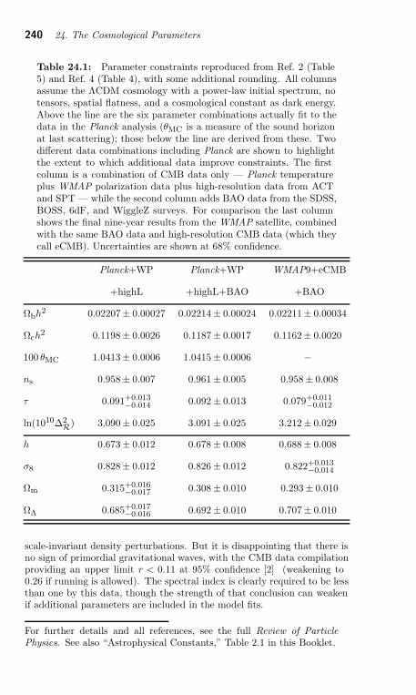
240 24. The Cosmological Parameters
Table 24.1: Parameter constraints reproduced from Ref. 2 (Table5) and Ref. 4 (Table 4), with some additional rounding. All columnsassume the ΛCDM cosmology with a power-law initial spectrum, notensors, spatial flatness, and a cosmological constant as dark energy.Above the line are the six parameter combinations actually fit to thedata in the Planck analysis (θMC is a measure of the sound horizonat last scattering); those below the line are derived from these. Twodifferent data combinations including Planck are shown to highlightthe extent to which additional data improve constraints. The firstcolumn is a combination of CMB data only — Planck temperatureplus WMAP polarization data plus high-resolution data from ACTand SPT — while the second column adds BAO data from the SDSS,BOSS, 6dF, and WiggleZ surveys. For comparison the last columnshows the final nine-year results from the WMAP satellite, combinedwith the same BAO data and high-resolution CMB data (which theycall eCMB). Uncertainties are shown at 68% confidence.
Planck+WP Planck+WP WMAP9+eCMB
+highL +highL+BAO +BAO
Ωbh2 0.02207± 0.00027 0.02214± 0.00024 0.02211± 0.00034
Ωch2 0.1198± 0.0026 0.1187± 0.0017 0.1162± 0.0020
100 θMC 1.0413± 0.0006 1.0415± 0.0006 −
ns 0.958± 0.007 0.961 ± 0.005 0.958± 0.008
τ 0.091+0.013−0.014
0.092 ± 0.013 0.079+0.011−0.012
ln(1010∆2R
) 3.090± 0.025 3.091 ± 0.025 3.212± 0.029
h 0.673± 0.012 0.678 ± 0.008 0.688± 0.008
σ8 0.828± 0.012 0.826 ± 0.012 0.822+0.013−0.014
Ωm 0.315+0.016−0.017
0.308 ± 0.010 0.293± 0.010
ΩΛ 0.685+0.017−0.016 0.692 ± 0.010 0.707± 0.010
scale-invariant density perturbations. But it is disappointing that there isno sign of primordial gravitational waves, with the CMB data compilationproviding an upper limit r < 0.11 at 95% confidence [2] (weakening to0.26 if running is allowed). The spectral index is clearly required to be lessthan one by this data, though the strength of that conclusion can weakenif additional parameters are included in the model fits.
For further details and all references, see the full Review of Particle
Physics. See also “Astrophysical Constants,” Table 2.1 in this Booklet.
25. Dark matter 241
25. DARK MATTER
Revised September 2013 by M. Drees (Bonn University) and G. Gerbier(Saclay, CEA).
25.1. Theory
25.1.1. Evidence for Dark Matter :
The existence of Dark (i.e., non-luminous and non-absorbing) Matter(DM) is by now well established [1,2]. An important example is themeasurement of galactic rotation curves. The rotational velocity v of anobject on a stable Keplerian orbit with radius r around a galaxy scaleslike v(r) ∝
√
M(r)/r, where M(r) is the mass inside the orbit. If r liesoutside the visible part of the galaxy and mass tracks light, one wouldexpect v(r) ∝ 1/
√r. Instead, in most galaxies one finds that v becomes
approximately constant out to the largest values of r where the rotationcurve can be measured. This implies the existence of a dark halo, withmass density ρ(r) ∝ 1/r2, i.e., M(r) ∝ r and a lower bound on the DMmass density, ΩDM
>∼ 0.1.
The observation of clusters of galaxies tends to give somewhat largervalues, ΩDM ≃ 0.2. These observations include measurements of thepeculiar velocities of galaxies in the cluster, which are a measure of theirpotential energy if the cluster is virialized; measurements of the X-ray
temperature of hot gas in the cluster, which again correlates with thegravitational potential felt by the gas; and—most directly—studies of(weak) gravitational lensing of background galaxies on the cluster.
The currently most accurate, if somewhat indirect, determination ofΩDM comes from global fits of cosmological parameters to a variety ofobservations; see the Section on Cosmological Parameters for details. Forexample, using measurements of the anisotropy of the cosmic microwavebackground (CMB) and of the spatial distribution of galaxies, Ref. 3 findsa density of cold, non-baryonic matter
Ωnbmh2 = 0.1198± 0.0026 , (25.1)
where h is the Hubble constant in units of 100 km/(s·Mpc). Some part ofthe baryonic matter density [3],
Ωbh2 = 0.02207± 0.00027 , (25.2)
may well contribute to (baryonic) DM, e.g., MACHOs [4] or cold moleculargas clouds [5].
The most recent estimate finds a quite similar result for the smoothcomponent of the local Dark Matter density [6]: (0.39 ± 0.03)GeVcm−3.
25.1.2. Candidates for Dark Matter :
Candidates for non-baryonic DM in Eq. (25.1) must satisfy severalconditions: they must be stable on cosmological time scales (otherwisethey would have decayed by now), they must interact very weaklywith electromagnetic radiation (otherwise they wouldn’t qualify as dark
matter), and they must have the right relic density. Candidates includeprimordial black holes, axions, sterile neutrinos, and weakly interactingmassive particles (WIMPs).
The existence of axions [10] was first postulated to solve the strongCP problem of QCD; they also occur naturally in superstring theories.They are pseudo Nambu-Goldstone bosons associated with the (mostly)spontaneous breaking of a new global “Peccei-Quinn” (PQ) U(1) symmetry
242 25. Dark matter
at scale fa; see the Section on Axions in this Review for further details.Although very light, axions would constitute cold DM, since they wereproduced non-thermally. At temperatures well above the QCD phasetransition, the axion is massless, and the axion field can take any value,parameterized by the “misalignment angle” θi. At T <∼ 1 GeV, the axiondevelops a mass ma ∼ fπmπ/fa due to instanton effects. Unless the axionfield happens to find itself at the minimum of its potential (θi = 0),it will begin to oscillate once ma becomes comparable to the Hubbleparameter H . These coherent oscillations transform the energy originallystored in the axion field into physical axion quanta. The contribution ofthis mechanism to the present axion relic density is [1]
Ωah2 = κa
(
fa/1012 GeV)1.175
θ2i , (25.5)
where the numerical factor κa lies roughly between 0.5 and a few.If θi ∼ O(1), Eq. (25.5) will saturate Eq. (25.1) for fa ∼ 1011 GeV,comfortably above laboratory and astrophysical constraints [10]; thiswould correspond to an axion mass around 0.1 meV. However, if the post-inflationary reheat temperature TR > fa, cosmic strings will form duringthe PQ phase transition at T ≃ fa. Their decay will give an additionalcontribution to Ωa, which is often bigger than that in Eq. (25.5) [1],leading to a smaller preferred value of fa, i.e., larger ma. On the otherhand, values of fa near the Planck scale become possible if θi is for somereason very small.
Weakly interacting massive particles (WIMPs) χ are particles withmass roughly between 10 GeV and a few TeV, and with cross sections ofapproximately weak strength. Within standard cosmology, their presentrelic density can be calculated reliably if the WIMPs were in thermaland chemical equilibrium with the hot “soup” of Standard Model (SM)particles after inflation. Their present relic density is then approximatelygiven by (ignoring logarithmic corrections) [12]
Ωχh2 ≃ const. · T 30
M3
Pl〈σAv〉
≃ 0.1 pb · c〈σAv〉 . (25.6)
Here T0 is the current CMB temperature, MPl is the Planck mass, c isthe speed of light, σA is the total annihilation cross section of a pairof WIMPs into SM particles, v is the relative velocity between the twoWIMPs in their cms system, and 〈. . .〉 denotes thermal averaging. Freezeout happens at temperature TF ≃ mχ/20 almost independently of theproperties of the WIMP. Notice that the 0.1 pb in Eq. (25.6) containsfactors of T0 and MPl; it is, therefore, quite intriguing that it “happens”to come out near the typical size of weak interaction cross sections.
The currently best motivated WIMP candidate is, therefore, the lightestsuperparticle (LSP) in supersymmetric models [13] with exact R-parity(which guarantees the stability of the LSP). Detailed calculations [1] showthat the lightest neutralino will have the desired thermal relic densityEq. (25.1) in at least four distinct regions of parameter space. χ could be(mostly) a bino or photino (the superpartner of the U(1)Y gauge bosonand photon, respectively), if both χ and some sleptons have mass below∼ 150 GeV, or if mχ is close to the mass of some sfermion (so that its relicdensity is reduced through co-annihilation with this sfermion), or if 2mχ
is close to the mass of the CP-odd Higgs boson present in supersymmetricmodels. Finally, Eq. (25.1) can also be satisfied if χ has a large higgsinoor wino component.
25. Dark matter 243
25.2. Experimental detection of Dark Matter
25.2.2. Axion searches :
Axions can be detected by looking for a → γ conversion in a strongmagnetic field [1]. Such a conversion proceeds through the loop-inducedaγγ coupling, whose strength gaγγ is an important parameter of axionmodels. There is currently only one experiment searching for axionic DM:the ADMX experiment [30], originally situated at the LLNL in Californiabut now running at the University of Washington, started taking data inthe first half of 1996. It employs a high quality cavity, whose “Q factor”enhances the conversion rate on resonance, i.e., for ma(c2 + v2
a/2) = ~ωres.One then needs to scan the resonance frequency in order to cover asignificant range in ma or, equivalently, fa.
25.2.4. Basics of direct WIMP search :
The WIMP mean velocity inside our galaxy relative to its center isexpected to be similar to that of stars, i.e., a few hundred kilometers persecond at the location of our solar system. For these velocities, WIMPsinteract with ordinary matter through elastic scattering on nuclei. Withexpected WIMP masses in the range 10 GeV to 10 TeV, typical nuclearrecoil energies are of order of 1 to 100 keV.
Expected interaction rates depend on the product of the local WIMPflux and the interaction cross section. The first term is fixed by the localdensity of dark matter, taken as 0.39 GeV/cm3, the mean WIMP velocity,typically 220 km/s, the galactic escape velocity, typically 544 km/s [26]and the mass of the WIMP. The expected interaction rate then mainlydepends on two unknowns, the mass and cross section of the WIMP (withsome uncertainty [6] due to the halo model). This is why the experimentalobservable, which is basically the scattering rate as a function of energy, isusually expressed as a contour in the WIMP mass–cross section plane.
The cross section depends on the nature of the couplings. For non-relativistic WIMPs, one in general has to distinguish spin-independentand spin-dependent couplings. The former can involve scalar and vectorWIMP and nucleon currents (vector currents are absent for MajoranaWIMPs, e.g., the neutralino), while the latter involve axial vector currents(and obviously only exist if χ carries spin). Due to coherence effects, thespin-independent cross section scales approximately as the square of themass of the nucleus, so higher mass nuclei, from Ge to Xe, are preferredfor this search. For spin-dependent coupling, the cross section depends onthe nuclear spin factor; used target nuclei include 19F, 23Na, 73Ge, 127I,129Xe, 131Xe, and 133Cs.
Cross sections calculated in MSSM models [27] induce rates of at most1 evt day−1 kg−1 of detector, much lower than the usual radioactivebackgrounds. This indicates the need for underground laboratories toprotect against cosmic ray induced backgrounds, and for the selection ofextremely radio-pure materials.
The typical shape of exclusion contours can be anticipated from thisdiscussion: at low WIMP mass, the sensitivity drops because of thedetector energy threshold, whereas at high masses, the sensitivity alsodecreases because, for a fixed mass density, the WIMP flux decreases∝ 1/mχ. The sensitivity is best for WIMP masses near the mass of therecoiling nucleus.
For further discussion and references, see the full Review.
244 26. Dark energy
26. DARK ENERGY
Written November 2013 by M. J. Mortonson (UCB, LBL), D. H. Weinberg(OSU), and M. White (UCB, LBL).
26.1. Repulsive Gravity and Cosmic Acceleration
In the late 1990s, supernova surveys by two independent teams provideddirect evidence for accelerating cosmic expansion [8,9], establishing thecosmological constant model (with Ωm ≈ 0.3, ΩΛ ≈ 0.7) as the preferredalternative to the Ωm = 1 scenario. Shortly thereafter, CMB evidencefor a spatially flat universe [10,11], and thus for Ωtot ≈ 1, cementedthe case for cosmic acceleration by firmly eliminating the free-expansionalternative with Ωm ≪ 1 and ΩΛ = 0. Today, the accelerating universeis well established by multiple lines of independent evidence from a tightweb of precise cosmological measurements.
As discussed in the Big Bang Cosmology article of this Review (Sec. 22),the scale factor R(t) of a homogeneous and isotropic universe governed by
GR grows at an accelerating rate if the pressure p < −13ρ. A cosmological
constant has ρΛ = const. and pressure pΛ = −ρΛ (see Eq. 22.10), so itwill drive acceleration if it dominates the total energy density. However,acceleration could arise from a more general form of “dark energy” thathas negative pressure, typically specified in terms of the equation-of-state-parameter w = p/ρ (= −1 for a cosmological constant). Furthermore, theconclusion that acceleration requires a new energy component beyondmatter and radiation relies on the assumption that GR is the correctdescription of gravity on cosmological scales.
26.2. Theories of Cosmic Acceleration
A cosmological constant is the mathematically simplest, and perhapsthe physically simplest, theoretical explanation for the acceleratinguniverse. The problem is explaining its unnaturally small magnitude, asdiscussed in Sec. 22.4.7 of this Review. An alternative (which still requiresfinding a way to make the cosmological constant zero or at least negligiblysmall) is that the accelerating cosmic expansion is driven by a new formof energy such as a scalar field [13] with potential V (φ). In the limit that1
2φ2 ≪ |V (φ)|, the scalar field acts like a cosmological constant, with
pφ ≈ −ρφ. In this scenario, today’s cosmic acceleration is closely akin tothe epoch of inflation, but with radically different energy and timescale.
More generally, the value of w = pφ/ρφ in scalar field models evolveswith time in a way that depends on V (φ) and on the initial conditions
(φi, φi); some forms of V (φ) have attractor solutions in which the late-timebehavior is insensitive to initial values. Many forms of time evolution arepossible, including ones where w is approximately constant and broadclasses where w “freezes” towards or “thaws” away from w = −1, withthe transition occurring when the field comes to dominate the totalenergy budget. If ρφ is even approximately constant, then it becomesdynamically insignificant at high redshift, because the matter densityscales as ρm ∝ (1 + z)3.
Further discussion and references may be found in the full Review of
Particle Physics.
27. Cosmic microwave background 245
27. COSMIC MICROWAVE BACKGROUND
Revised Sept. 2013 by D. Scott (U. of BC) and G.F. Smoot (UCB/LBNL).
27.2. Description of CMB Anisotropies
Observations show that the CMB contains anisotropies at the 10−5
level, over a wide range of angular scales. These anisotropies are usuallyexpressed by using a spherical harmonic expansion of the CMB sky:
T (θ, φ) =∑
ℓm
aℓmYℓm(θ, φ).
The vast majority of the cosmological information is contained in thetemperature 2-point function, i.e., the variance as a function only ofangular separation, since we notice no preferred direction. Equivalently,the power per unit ln ℓ is ℓ
∑
m |aℓm|2 /4π.
27.2.1. The Monopole :The CMB has a mean temperature of Tγ = 2.7255 ± 0.0006 K (1σ) [15]
, which can be considered as the monopole component of CMB maps,a00. Since all mapping experiments involve difference measurements,they are insensitive to this average level. Monopole measurementscan only be made with absolute temperature devices, such as theFIRAS instrument on the COBE satellite [16] . Such measurementsof the spectrum are consistent with a blackbody distribution overmore than three decades in frequency (with some recent suggestionsof a possible deviation at low frequencies [17]) . A blackbody of themeasured temperature corresponds to nγ = (2ζ(3)/π2)T 3
γ ≃ 411 cm−3 and
ργ = (π2/15)T 4γ ≃ 4.64 × 10⁻³⁴ g cm−3 ≃ 0.260 eVcm−3.
27.2.2. The Dipole :The largest anisotropy is in the ℓ = 1 (dipole) first spherical harmonic,
with amplitude 3.355 ± 0.008 mK [7]. The dipole is interpreted to be theresult of the Doppler shift caused by the solar system motion relative to thenearly isotropic blackbody field, as broadly confirmed by measurements ofthe radial velocities of local galaxies (although with some debate [18]) .
The dipole is a frame-dependent quantity, and one can thus determinethe ‘absolute rest frame’ as that in which the CMB dipole would be zero.
27.2.3. Higher-Order Multipoles :The variations in the CMB temperature maps at higher multipoles
(ℓ ≥ 2) are interpreted as being mostly the result of perturbations in thedensity of the early Universe, manifesting themselves at the epoch of thelast scattering of the CMB photons. In the hot Big Bang picture, theexpansion of the Universe cools the plasma so that by a redshift z ≃ 1100(with little dependence on the details of the model), the hydrogen andhelium nuclei can bind electrons into neutral atoms, a process usuallyreferred to as recombination [22]. Before this epoch, the CMB photonswere tightly coupled to the baryons, while afterwards they could freelystream towards us. By measuring the aℓms we are thus learning directlyabout physical conditions in the early Universe.
A statistically isotropic sky means that all ms are equivalent, i.e., thereis no preferred axis, so that the temperature correlation function betweentwo positions on the sky depends only on angular separation and notorientation. Together with the assumption of Gaussian statistics (i.e. nocorrelations between the modes), the variance of the temperature field(or equivalently the power spectrum in ℓ) then fully characterizes the
246 27. Cosmic microwave background
anisotropies. The power summed over all ms at each ℓ is (2ℓ + 1)Cℓ/(4π),where Cℓ ≡
⟨
|aℓm|2⟩
. Thus averages of aℓms over m can be used asestimators of the Cℓs to constrain their expectation values, which arethe quantities predicted by a theoretical model. For an idealized full-skyobservation, the variance of each measured Cℓ (i.e., the variance ofthe variance) is [2/(2ℓ + 1)]C2
ℓ . This sampling uncertainty (known as
‘cosmic variance’) comes about because each Cℓ is χ2 distributed with(2ℓ + 1) degrees of freedom for our observable volume of the Universe. Forfractional sky coverage, fsky, this variance is increased by 1/fsky and themodes become partially correlated.
It is important to understand that theories predict the expectationvalue of the power spectrum, whereas our sky is a single realization.Hence the cosmic variance is an unavoidable source of uncertainty whenconstraining models; it dominates the scatter at lower ℓs, while the effectsof instrumental noise and resolution dominate at higher ℓs [23].
Theoretical models generally predict that the aℓm modes are Gaussianrandom fields to high precision, matching the empirical tests, e.g., standardslow-roll inflation’s non-Gaussian contribution is expected to be at leastan order of magnitude below current observational limits [24]. Althoughnon-Gaussianity of various forms is possible in early Universe models, testsshow that Gaussianity is an extremely good simplifying approximation [25]. The only current indications of any non-Gaussianity or statisticalanisotropy are some relatively weak signatures at large scales, seen in bothWMAP [26] and Planck data [27], but not of high enough significance toreject the simplifying assumption.
27.2.4. Angular Resolution and Binning :There is no one-to-one conversion between multipole ℓ and the angle
subtended by a particular spatial scale projected onto the sky. However,a single spherical harmonic Yℓm corresponds to angular variations ofθ ∼ π/ℓ. CMB maps contain anisotropy information from the size of themap (or in practice some fraction of that size) down to the beam-sizeof the instrument, σ (the standard deviation of the beam, in radians).One can think of the effect of a Gaussian beam as rolling off the power
spectrum with the function e−ℓ(ℓ+1)σ2
.
27.5. Current Temperature Anisotropy Data
There has been a steady improvement in the quality of CMB datathat has led to the development of the present-day cosmological model.Probably the most robust constraints currently available come from Plancksatellite [43] data combined with smaller scale results from the ACT [44]and SPT [45] experiments (together with constraints from non-CMBcosmological data-sets). We plot power spectrum estimates from theseexperiments in Fig. 27.1, along with WMAP data to show the consistency(see previous versions of this review for data from earlier experiments).
27.6. CMB Polarization
Since Thomson scattering of an anisotropic radiation field also generateslinear polarization, the CMB is predicted to be polarized at the levelof roughly 5% of the temperature anisotropies [46] . Polarization is aspin-2 field on the sky, and the algebra of the modes in ℓ-space isstrongly analogous to spin-orbit coupling in quantum mechanics [47] .The linear polarization pattern can be decomposed in a number of ways,with two quantities required for each pixel in a map, often given as theQ and U Stokes parameters. However, the most intuitive and physical
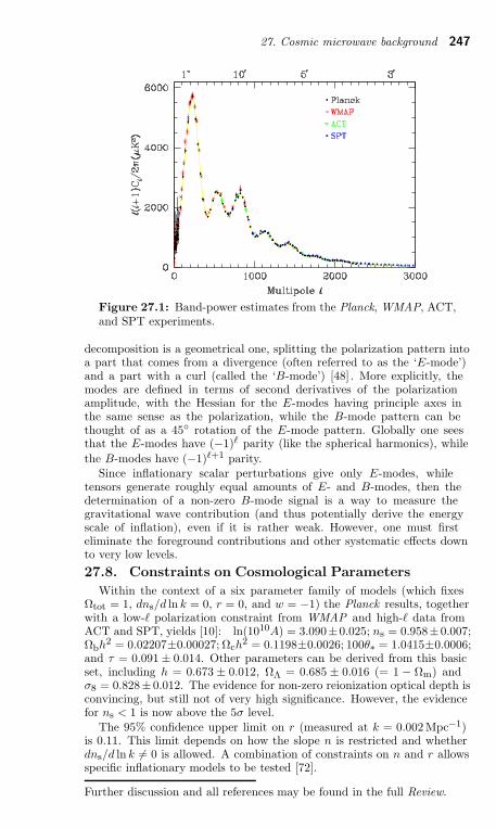
27. Cosmic microwave background 247
Figure 27.1: Band-power estimates from the Planck, WMAP, ACT,and SPT experiments.
decomposition is a geometrical one, splitting the polarization pattern intoa part that comes from a divergence (often referred to as the ‘E-mode’)and a part with a curl (called the ‘B-mode’) [48] . More explicitly, themodes are defined in terms of second derivatives of the polarizationamplitude, with the Hessian for the E-modes having principle axes inthe same sense as the polarization, while the B-mode pattern can bethought of as a 45 rotation of the E-mode pattern. Globally one seesthat the E-modes have (−1)ℓ parity (like the spherical harmonics), while
the B-modes have (−1)ℓ+1 parity.Since inflationary scalar perturbations give only E-modes, while
tensors generate roughly equal amounts of E- and B-modes, then thedetermination of a non-zero B-mode signal is a way to measure thegravitational wave contribution (and thus potentially derive the energyscale of inflation), even if it is rather weak. However, one must firsteliminate the foreground contributions and other systematic effects downto very low levels.
27.8. Constraints on Cosmological Parameters
Within the context of a six parameter family of models (which fixesΩtot = 1, dns/d ln k = 0, r = 0, and w = −1) the Planck results, togetherwith a low-ℓ polarization constraint from WMAP and high-ℓ data fromACT and SPT, yields [10]: ln(1010A) = 3.090±0.025; ns = 0.958±0.007;Ωbh2 = 0.02207±0.00027; Ωch
2 = 0.1198±0.0026; 100θ∗ = 1.0415±0.0006;and τ = 0.091 ± 0.014. Other parameters can be derived from this basicset, including h = 0.673 ± 0.012, ΩΛ = 0.685 ± 0.016 (= 1 − Ωm) andσ8 = 0.828± 0.012. The evidence for non-zero reionization optical depth isconvincing, but still not of very high significance. However, the evidencefor ns < 1 is now above the 5σ level.
The 95% confidence upper limit on r (measured at k = 0.002 Mpc−1)is 0.11. This limit depends on how the slope n is restricted and whetherdns/d ln k 6= 0 is allowed. A combination of constraints on n and r allowsspecific inflationary models to be tested [72].
Further discussion and all references may be found in the full Review.
248 28. Cosmic rays
28. COSMIC RAY FLUXES∗
In the lower half of the atmosphere (altitude <∼ 5 km) most cosmic rays
are muons. Some typical sea-level values for charged particles are givenbelow, where
Iv flux per unit solid angle per unit horizontal area about verticaldirection≡ j(θ = 0, φ)[θ = zenith angle, φ = azimuthal angle] ;
J1 total flux crossing unit horizontal area from above
≡
∫θ≤π/2
j(θ, φ) cos θ dΩ [dΩ = sin θ dθ dφ] ;
J2 total flux from above (crossing a sphere of unit cross-sectional area)
≡
∫θ≤π/2
j(θ, φ) dΩ .
Total Hard (≈ µ±) Soft (≈ e±)Intensity Component Component
Iv 110 80 30 m−2 s−1 sr−1
J1 180 130 50 m−2 s−1
J2 240 170 70 m−2 s−1
At 4300 m (e.g., Mt. Evans or Mauna Kea) the hard component is 2.3times more intense than at sea level.
The p/µ± vertical flux ratio at sea level is about 3.5% at 1 GeV/c,decreasing to about 0.5% at 10 GeV/c. The π±/µ± ratio is an order ofmagnitude smaller.
The mean energy of muons at the ground is ≈ 4 GeV. The energyspectrum is almost flat below 1 GeV, steepens gradually to reflect theprimary spectrum (∝ E−2.7) in the 10–100 GeV range, and asymptoticallybecomes one power steeper (Eµ ≫ 1 TeV). The measurements reportedabove are for Eµ >
∼ 225 MeV. The angular distribution is very nearly
proportional to cos2 θ, changing to sec θ at energies above a TeV (where θis the zenith angle at production). The µ+/µ− ratio is 1.25–1.30.
The mean energy of muons originating in the atmosphere is roughly300 GeV at slant depths underground & a few hundred meters. Beyondslant depths of ≈ 10 km water-equivalent, the muons are due primarily toin-the-earth neutrino interactions (roughly 1/8 interaction ton−1 yr−1 forEν > 300 MeV, ≈ constant throughout the earth). These muons arrivedwith a mean energy of 20 GeV, and have a flux of 2 × 10⁻⁹ m−2 s−1 sr−1
in the vertical direction and about twice that in the horizontal, down atleast as far as the deepest mines.
∗ Reprint of “Cosmic-ray fluxes” from the 1986 Review, as updated byD.E. Groom (2000). The data (by Greisen) are reported in B. Rossi,Rev. Mod. Phys. 20, 537 (1948). See the full Review on Cosmic Raysfor a more extensive discussion and references.
29. Accelerator physics of colliders 249
29. ACCELERATOR PHYSICS OF COLLIDERS
Revised August 2013 by M.J. Syphers (MSU) and F. Zimmermann (CERN)
29.1. Luminosity
The number of events, Nexp, is the product of the cross section ofinterest, σexp, and the time integral over the instantaneous luminosity, L :
Nexp = σexp ×
∫
L (t)dt. (29.1)
If two bunches containing n1 and n2 particles collide head-on withfrequency f , a basic expression for the luminosity is
L = fn1n2
4πσxσy
(29.2)
where σx and σy characterize the rms transverse beam sizes in thehorizontal (bend) and vertical directions. In this form it is assumedthat the bunches are identical in transverse profile, that the profilesare Gaussian and independent of position along the bunch, and theparticle distributions are not altered during bunch crossing. Nonzero beamcrossing angles and long bunches will reduce the luminosity from thisvalue.
Whatever the distribution at the source, by the time the beam reacheshigh energy, the normal form is a useful approximation as suggested bythe σ-notation.
The beam size can be expressed in terms of two quantities, one termedthe transverse emittance, ǫ, and the other, the amplitude function, β. Thetransverse emittance is a beam quality concept reflecting the process ofbunch preparation, extending all the way back to the source for hadronsand, in the case of electrons, mostly dependent on synchrotron radiation.The amplitude function is a beam optics quantity and is determined bythe accelerator magnet configuration. When expressed in terms of σ andβ the transverse emittance becomes
ǫ = σ2/β .
Of particular significance is the value of the amplitude function at theinteraction point, β∗. Clearly one wants β∗ to be as small as possible; howsmall depends on the capability of the hardware to make a near-focus atthe interaction point.
Eq. (29.2) can now be recast in terms of emittances and amplitudefunctions as
L = fn1n2
4π√
ǫx β∗
x ǫy β∗
y
. (29.10)
Thus, to achieve high luminosity, all one has to do is make high populationbunches of low emittance to collide at high frequency at locations wherethe beam optics provides as low values of the amplitude functions aspossible.
Further discussion and references may be found in the full Review of
Particle Physics.
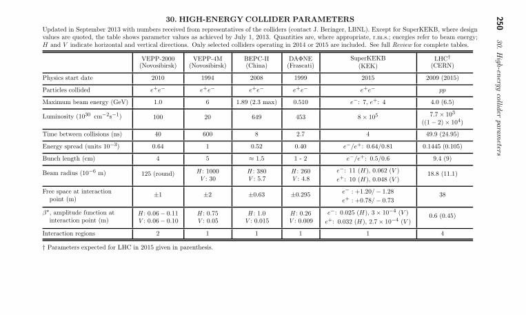
250
30.H
igh-e
nerg
yco
llider
para
mete
rs30. HIGH-ENERGY COLLIDER PARAMETERS
Updated in September 2013 with numbers received from representatives of the colliders (contact J. Beringer, LBNL). Except for SuperKEKB, where designvalues are quoted, the table shows parameter values as achieved by July 1, 2013. Quantities are, where appropriate, r.m.s.; energies refer to beam energy;H and V indicate horizontal and vertical directions. Only selected colliders operating in 2014 or 2015 are included. See full Review for complete tables.
VEPP-2000(Novosibirsk)
VEPP-4M(Novosibirsk)
BEPC-II(China)
DAΦNE(Frascati)
SuperKEKB(KEK)
LHC†
(CERN)
Physics start date 2010 1994 2008 1999 2015 2009 (2015)
Particles collided e+e− e+e− e+e− e+e− e+e− pp
Maximum beam energy (GeV) 1.0 6 1.89 (2.3 max) 0.510 e−: 7, e+: 4 4.0 (6.5)
Luminosity (1030 cm−2s−1) 100 20 649 453 8 × 10⁵ 7.7 × 10³
((1 − 2) × 104)
Time between collisions (ns) 40 600 8 2.7 4 49.9 (24.95)
Energy spread (units 10−3) 0.64 1 0.52 0.40 e−/e+: 0.64/0.81 0.1445 (0.105)
Bunch length (cm) 4 5 ≈ 1.5 1 - 2 e−/e+: 0.5/0.6 9.4 (9)
Beam radius (10−6 m) 125 (round) H : 1000V : 30
H : 380V : 5.7
H : 260V : 4.8
e−: 11 (H), 0.062 (V )
e+: 10 (H), 0.048 (V )18.8 (11.1)
Free space at interactionpoint (m)
±1 ±2 ±0.63 ±0.295 e− : +1.20/− 1.28
e+ : +0.78/− 0.7338
β∗, amplitude function atinteraction point (m)
H : 0.06 − 0.11V : 0.06 − 0.10
H : 0.75V : 0.05
H : 1.0V : 0.015
H : 0.26V : 0.009
e−: 0.025 (H), 3 × 10⁻⁴ (V )
e+: 0.032 (H), 2.7 × 10⁻⁴ (V )0.6 (0.45)
Interaction regions 2 1 1 1 1 4
† Parameters expected for LHC in 2015 given in parenthesis.
32. Passage of particles through matter 251
32. PASSAGE OF PARTICLES THROUGH MATTER
Revised September 2013 by H. Bichsel (University of Washington), D.E.Groom (LBNL), and S.R. Klein (LBNL).
32.1. NotationTable 32.1: Summary of variables used in this section. Thekinematic variables β and γ have their usual relativistic meanings.
Symbol Definition Value or (usual) units
α fine structure constant
e2/4πǫ0~c 1/137.035 999 074(44)
M incident particle mass MeV/c2
E incident part. energy γMc2 MeV
T kinetic energy, (γ − 1)Mc2 MeV
W energy transfer to an electron MeV
in a single collision
k bremsstrahlung photon energy MeV
mec2 electron mass × c2 0.510 998 928(11) MeV
re classical electron radius
e2/4πǫ0mec2 2.817 940 3267(27) fm
NA Avogadro’s number 6.022 141 29(27)× 1023 mol−1
z charge number of incident particle
Z atomic number of absorber
A atomic mass of absorber g mol−1
K 4πNAr2emec
2 0.307 075 MeV mol−1 cm2
I mean excitation energy eV (Nota bene!)
δ(βγ) density effect correction to ionization energy loss
~ωp plasma energy√
ρ 〈Z/A〉 × 28.816 eV√
4πNer3e mec
2/α |−→ ρ in g cm−3
Ne electron density (units of re)−3
wj weight fraction of the jth element in a compound or mixture
nj ∝ number of jth kind of atoms in a compound or mixture
X0 radiation length g cm−2
Ec critical energy for electrons MeV
Eµc critical energy for muons GeV
Es scale energy√
4π/α mec2 21.2052 MeV
RM Moliere radius g cm−2
32.2. Electronic energy loss by heavy particles [1–33]
32.2.1. Moments and cross sections :The electronic interactions of fast charged particles with speed v = βc
occur in single collisions with energy losses E [1], leading to ionization,atomic, or collective excitation. Most frequently the energy losses aresmall (for 90% of all collisions the energy losses are less than 100 eV). Inthin absorbers few collisions will take place and the total energy loss willshow a large variance [1]; also see Sec. 32.2.9 below. For particles withcharge ze more massive than electrons (“heavy” particles), scattering fromfree electrons is adequately described by the Rutherford differential cross
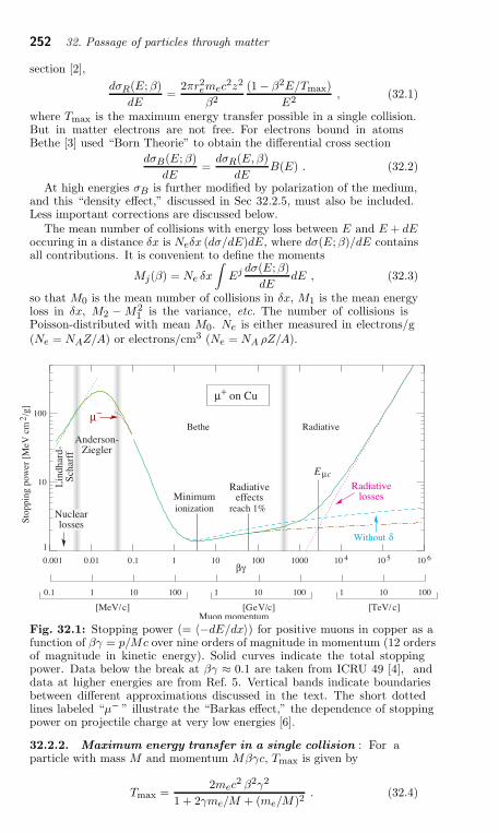
252 32. Passage of particles through matter
section [2],
dσR(E; β)
dE=
2πr2emec
2z2
β2
(1 − β2E/Tmax)
E2, (32.1)
where Tmax is the maximum energy transfer possible in a single collision.But in matter electrons are not free. For electrons bound in atomsBethe [3] used “Born Theorie” to obtain the differential cross section
dσB(E; β)
dE=
dσR(E, β)
dEB(E) . (32.2)
At high energies σB is further modified by polarization of the medium,and this “density effect,” discussed in Sec 32.2.5, must also be included.Less important corrections are discussed below.
The mean number of collisions with energy loss between E and E + dEoccuring in a distance δx is Neδx (dσ/dE)dE, where dσ(E; β)/dE containsall contributions. It is convenient to define the moments
Mj(β) = Ne δx
∫
Ej dσ(E; β)
dEdE , (32.3)
so that M0 is the mean number of collisions in δx, M1 is the mean energyloss in δx, M2 − M2
1 is the variance, etc. The number of collisions isPoisson-distributed with mean M0. Ne is either measured in electrons/g(Ne = NAZ/A) or electrons/cm3 (Ne = NA ρZ/A).
Fig. 32.1: Stopping power (= 〈−dE/dx〉) for positive muons in copper as afunction of βγ = p/Mc over nine orders of magnitude in momentum (12 ordersof magnitude in kinetic energy). Solid curves indicate the total stoppingpower. Data below the break at βγ ≈ 0.1 are taken from ICRU 49 [4], anddata at higher energies are from Ref. 5. Vertical bands indicate boundariesbetween different approximations discussed in the text. The short dottedlines labeled “µ− ” illustrate the “Barkas effect,” the dependence of stoppingpower on projectile charge at very low energies [6].
32.2.2. Maximum energy transfer in a single collision : For aparticle with mass M and momentum Mβγc, Tmax is given by
Tmax =2mec
2 β2γ2
1 + 2γme/M + (me/M)2. (32.4)
32. Passage of particles through matter 253
In older references [2,8] the “low-energy” approximation Tmax =2mec
2 β2γ2, valid for 2γme/M ≪ 1, is often implicit. For hadrons withE ≃ 100 GeV, it is limited by structure effects.
32.2.3. Stopping power at intermediate energies : The mean rateof energy loss by moderately relativistic charged heavy particles, M1/δx,is well-described by the “Bethe” equation,
−⟨
dE
dx
⟩
= Kz2Z
A
1
β2
[
1
2ln
2mec2β2γ2Tmax
I2− β2 − δ(βγ)
2
]
. (32.5)
It describes the mean loss rate in the region 0.1 <∼ βγ <∼ 1000 forintermediate-Z materials with an accuracy of a few %. At the lower limitthe projectile velocity becomes comparable to atomic electron “velocities”(Sec. 32.2.4), and at the upper limit radiative effects begin to be important(Sec. 32.6). Both limits are Z dependent. Here Tmax is the maximumkinetic energy which can be imparted to a free electron in a single collision,and the other variables are defined in Table 32.1. A minor dependenceon M at the highest energies is introduced through Tmax, but for allpractical purposes 〈dE/dx〉 in a given material is a function of β alone.With definitions and values in Table 32.1, the units are MeV g−1cm2.
Few concepts in high-energy physics are as misused as 〈dE/dx〉. Themain problem is that the mean is weighted by very rare events with largesingle-collision energy deposits. Even with samples of hundreds of events adependable value for the mean energy loss cannot be obtained. Far betterand more easily measured is the most probable energy loss, discussed inSec 32.2.9. It is considerably below the mean given by the Bethe equation.
In a TPC (Sec. 33.6.5), the mean of 50%–70% of the samples with thesmallest signals is often used as an estimator.
Although it must be used with cautions and caveats, 〈dE/dx〉 asdescribed in Eq. (32.5) still forms the basis of much of our understandingof energy loss by charged particles. Extensive tables are available[4,5,pdg.lbl.gov/AtomicNuclearProperties/].
The function as computed for muons on copper is shown as the“Bethe” region of Fig. 32.1. Mean energy loss behavior below this regionis discussed in Sec. 32.2.6, and the radiative effects at high energy arediscussed in Sec. 32.6. Only in the Bethe region is it a function of β alone;the mass dependence is more complicated elsewhere. The stopping powerin several other materials is shown in Fig. 32.2. Except in hydrogen,particles with the same velocity have similar rates of energy loss in differentmaterials, although there is a slow decrease in the rate of energy loss withincreasing Z. The qualitative behavior difference at high energies betweena gas (He in the figure) and the other materials shown in the figureis due to the density-effect correction, δ(βγ), discussed in Sec. 32.2.5.The stopping power functions are characterized by broad minima whoseposition drops from βγ = 3.5 to 3.0 as Z goes from 7 to 100. The values ofminimum ionization go roughly as 0.235 − 0.28 ln(Z), in MeVg−1cm−2,for Z > 6.
Eq. (32.5) may be integrated to find the total (or partial) “continuousslowing-down approximation” (CSDA) range R for a particle which losesenergy only through ionization and atomic excitation. Since dE/dx inthe “Bethe region” depends only on β, R/M is a function of E/M orpc/M . In practice, range is a useful concept only for low-energy hadrons(R <∼ λI , where λI is the nuclear interaction length), and for muons belowa few hundred GeV (above which radiative effects dominate). R/M as afunction of βγ = p/Mc is shown for a variety of materials in Fig. 32.4.
The mass scaling of dE/dx and range is valid for the electronic losses
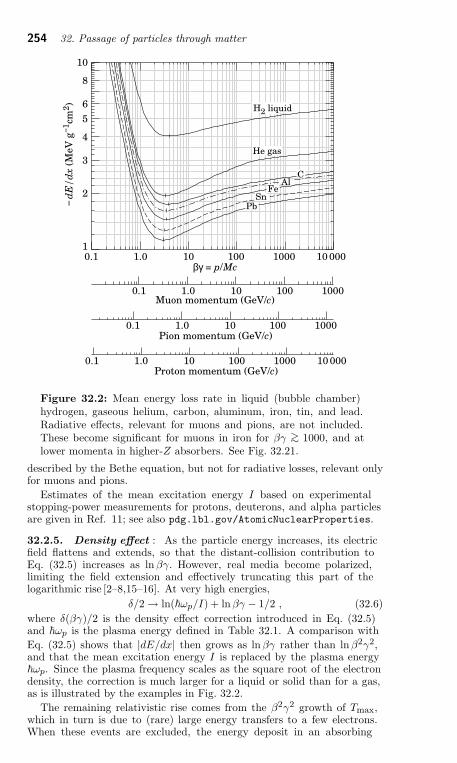
254 32. Passage of particles through matter
1
2
3
4
5
6
8
10
1.0 10 100 1000 10 0000.1
Pion momentum (GeV/c)
Proton momentum (GeV/c)
1.0 10 100 10000.1
1.0 10 100 10000.1
1.0 10 100 1000 10 0000.1
−dE/dx (
MeV
g−1
cm2)
βγ = p/Mc
Muon momentum (GeV/c)
H2 liquid
He gas
CAl
FeSn
Pb
Figure 32.2: Mean energy loss rate in liquid (bubble chamber)hydrogen, gaseous helium, carbon, aluminum, iron, tin, and lead.Radiative effects, relevant for muons and pions, are not included.These become significant for muons in iron for βγ >∼ 1000, and atlower momenta in higher-Z absorbers. See Fig. 32.21.
described by the Bethe equation, but not for radiative losses, relevant onlyfor muons and pions.
Estimates of the mean excitation energy I based on experimentalstopping-power measurements for protons, deuterons, and alpha particlesare given in Ref. 11; see also pdg.lbl.gov/AtomicNuclearProperties.
32.2.5. Density effect : As the particle energy increases, its electricfield flattens and extends, so that the distant-collision contribution toEq. (32.5) increases as ln βγ. However, real media become polarized,limiting the field extension and effectively truncating this part of thelogarithmic rise [2–8,15–16]. At very high energies,
δ/2 → ln(~ωp/I) + lnβγ − 1/2 , (32.6)
where δ(βγ)/2 is the density effect correction introduced in Eq. (32.5)and ~ωp is the plasma energy defined in Table 32.1. A comparison with
Eq. (32.5) shows that |dE/dx| then grows as ln βγ rather than lnβ2γ2,and that the mean excitation energy I is replaced by the plasma energy~ωp. Since the plasma frequency scales as the square root of the electrondensity, the correction is much larger for a liquid or solid than for a gas,as is illustrated by the examples in Fig. 32.2.
The remaining relativistic rise comes from the β2γ2 growth of Tmax,which in turn is due to (rare) large energy transfers to a few electrons.When these events are excluded, the energy deposit in an absorbing
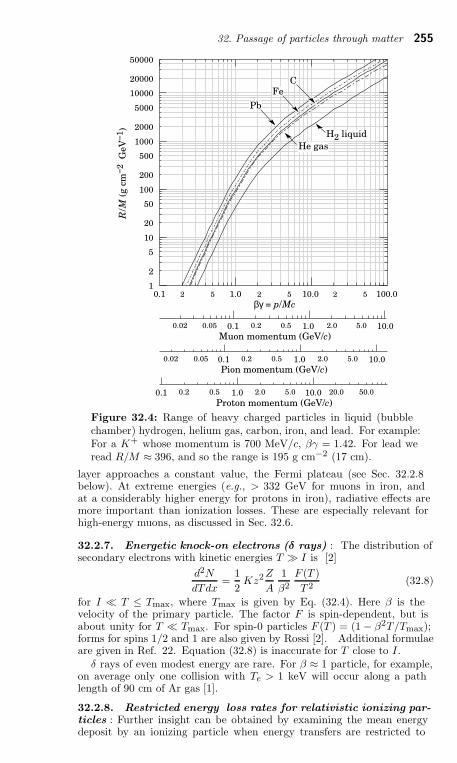
32. Passage of particles through matter 255
0.05 0.10.02 0.50.2 1.0 5.02.0 10.0
Pion momentum (GeV/c)
0.1 0.50.2 1.0 5.02.0 10.0 50.020.0
Proton momentum (GeV/c)
0.050.02 0.1 0.50.2 1.0 5.02.0 10.0
Muon momentum (GeV/c)
βγ = p/Mc
1
2
5
10
20
50
100
200
500
1000
2000
5000
10000
20000
50000
R/M
(g c
m−2
G
eV
−1)
0.1 2 5 1.0 2 5 10.0 2 5 100.0
H2 liquid
He gas
Pb
FeC
Figure 32.4: Range of heavy charged particles in liquid (bubblechamber) hydrogen, helium gas, carbon, iron, and lead. For example:For a K+ whose momentum is 700 MeV/c, βγ = 1.42. For lead weread R/M ≈ 396, and so the range is 195 g cm−2 (17 cm).
layer approaches a constant value, the Fermi plateau (see Sec. 32.2.8below). At extreme energies (e.g., > 332 GeV for muons in iron, andat a considerably higher energy for protons in iron), radiative effects aremore important than ionization losses. These are especially relevant forhigh-energy muons, as discussed in Sec. 32.6.
32.2.7. Energetic knock-on electrons (δ rays) : The distribution ofsecondary electrons with kinetic energies T ≫ I is [2]
d2N
dTdx=
1
2Kz2Z
A
1
β2
F (T )
T 2(32.8)
for I ≪ T ≤ Tmax, where Tmax is given by Eq. (32.4). Here β is thevelocity of the primary particle. The factor F is spin-dependent, but isabout unity for T ≪ Tmax. For spin-0 particles F (T ) = (1 − β2T/Tmax);forms for spins 1/2 and 1 are also given by Rossi [2]. Additional formulaeare given in Ref. 22. Equation (32.8) is inaccurate for T close to I.
δ rays of even modest energy are rare. For β ≈ 1 particle, for example,on average only one collision with Te > 1 keV will occur along a pathlength of 90 cm of Ar gas [1].
32.2.8. Restricted energy loss rates for relativistic ionizing par-ticles : Further insight can be obtained by examining the mean energydeposit by an ionizing particle when energy transfers are restricted to
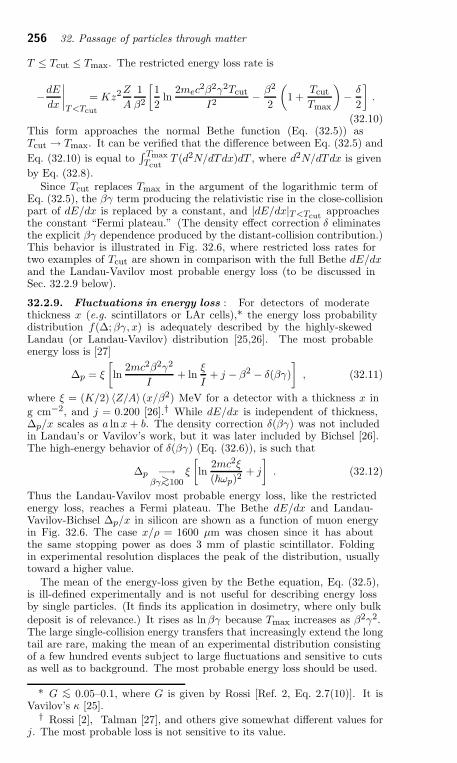
256 32. Passage of particles through matter
T ≤ Tcut ≤ Tmax. The restricted energy loss rate is
−dE
dx
∣
∣
∣
∣
T<Tcut
= Kz2Z
A
1
β2
[
1
2ln
2mec2β2γ2Tcut
I2− β2
2
(
1 +Tcut
Tmax
)
− δ
2
]
.
(32.10)This form approaches the normal Bethe function (Eq. (32.5)) asTcut → Tmax. It can be verified that the difference between Eq. (32.5) and
Eq. (32.10) is equal to∫ Tmax
TcutT (d2N/dTdx)dT , where d2N/dTdx is given
by Eq. (32.8).Since Tcut replaces Tmax in the argument of the logarithmic term of
Eq. (32.5), the βγ term producing the relativistic rise in the close-collisionpart of dE/dx is replaced by a constant, and |dE/dx|T<Tcut
approachesthe constant “Fermi plateau.” (The density effect correction δ eliminatesthe explicit βγ dependence produced by the distant-collision contribution.)This behavior is illustrated in Fig. 32.6, where restricted loss rates fortwo examples of Tcut are shown in comparison with the full Bethe dE/dxand the Landau-Vavilov most probable energy loss (to be discussed inSec. 32.2.9 below).
32.2.9. Fluctuations in energy loss : For detectors of moderatethickness x (e.g. scintillators or LAr cells),* the energy loss probabilitydistribution f(∆; βγ, x) is adequately described by the highly-skewedLandau (or Landau-Vavilov) distribution [25,26]. The most probableenergy loss is [27]
∆p = ξ
[
ln2mc2β2γ2
I+ ln
ξ
I+ j − β2 − δ(βγ)
]
, (32.11)
where ξ = (K/2) 〈Z/A〉 (x/β2) MeV for a detector with a thickness x in
g cm−2, and j = 0.200 [26].† While dE/dx is independent of thickness,∆p/x scales as a lnx + b. The density correction δ(βγ) was not includedin Landau’s or Vavilov’s work, but it was later included by Bichsel [26].The high-energy behavior of δ(βγ) (Eq. (32.6)), is such that
∆p −→βγ>∼100
ξ
[
ln2mc2ξ
(~ωp)2+ j
]
. (32.12)
Thus the Landau-Vavilov most probable energy loss, like the restrictedenergy loss, reaches a Fermi plateau. The Bethe dE/dx and Landau-Vavilov-Bichsel ∆p/x in silicon are shown as a function of muon energyin Fig. 32.6. The case x/ρ = 1600 µm was chosen since it has aboutthe same stopping power as does 3 mm of plastic scintillator. Foldingin experimental resolution displaces the peak of the distribution, usuallytoward a higher value.
The mean of the energy-loss given by the Bethe equation, Eq. (32.5),is ill-defined experimentally and is not useful for describing energy lossby single particles. (It finds its application in dosimetry, where only bulkdeposit is of relevance.) It rises as ln βγ because Tmax increases as β2γ2.The large single-collision energy transfers that increasingly extend the longtail are rare, making the mean of an experimental distribution consistingof a few hundred events subject to large fluctuations and sensitive to cutsas well as to background. The most probable energy loss should be used.
* G <∼ 0.05–0.1, where G is given by Rossi [Ref. 2, Eq. 2.7(10)]. It isVavilov’s κ [25].
† Rossi [2], Talman [27], and others give somewhat different values forj. The most probable loss is not sensitive to its value.
32. Passage of particles through matter 257
Landau/Vavilov/Bichsel ∆p/x for :
Bethe
Tcut = 10 dE/dx|minTcut = 2 dE/dx|min
Restricted energy loss for :
0.1 1.0 10.0 100.0 1000.0
1.0
1.5
0.5
2.0
2.5
3.0
MeV
g−1
cm
2 (E
lect
roni
c lo
sses
onl
y)
Muon kinetic energy (GeV)
Silicon
x/ρ = 1600 µm320 µm80 µm
Figure 32.6: Bethe dE/dx, two examples of restricted energyloss, and the Landau most probable energy per unit thickness insilicon. The change of ∆p/x with thickness x illustrates its a lnx + bdependence. Minimum ionization (dE/dx|min) is 1.664 MeV g−1 cm2.Radiative losses are excluded. The incident particles are muons.
For very thick absorbers the distribution is less skewed but neverapproaches a Gaussian. In the case of Si illustrated in Fig. 32.6, the mostprobable energy loss per unit thickness for x ≈ 35 g cm−2 is very close tothe restricted energy loss with Tcut = 2 dE/dx|min.
The Landau distribution fails to describe energy loss in thin absorberssuch as gas TPC cells [1] and Si detectors [26], as shown clearly inFig. 1 of Ref. 1 for an argon-filled TPC cell. Also see Talman [27]. While∆p/x may be calculated adequately with Eq. (32.11), the distributionsare significantly wider than the Landau width w = 4ξ [Ref. 26, Fig. 15].Examples for thin silicon detectors are shown in Fig. 32.8.
32.2.10. Energy loss in mixtures and compounds : A mixture orcompound can be thought of as made up of thin layers of pure elementsin the right proportion (Bragg additivity). In this case,
dE
dx=
∑
wjdE
dx
∣
∣
∣
∣
j, (32.13)
where dE/dx|j is the mean rate of energy loss (in MeV g cm−2)in the jth element. Eq. (32.5) can be inserted into Eq. (32.13) tofind expressions for 〈Z/A〉, 〈I 〉, and 〈δ〉; for example, 〈Z/A〉 =∑
wjZj/Aj =∑
njZj/∑
njAj . However, 〈I 〉 as defined this way isan underestimate, because in a compound electrons are more tightlybound than in the free elements, and 〈δ〉 as calculated this way has littlerelevance, because it is the electron density that matters. If possible,one uses the tables given in Refs. 16 and 29, or the recipes given in17 (repeated in Ref. 5), which include effective excitation energies andinterpolation coefficients for calculating the density effect correction.
32.3. Multiple scattering through small angles
A charged particle traversing a medium is deflected by many small-anglescatters. Most of this deflection is due to Coulomb scattering from nuclei,and hence the effect is called multiple Coulomb scattering. (However, forhadronic projectiles, the strong interactions also contribute to multiplescattering.) The Coulomb scattering distribution is well represented by the
258 32. Passage of particles through matter
theory of Moliere [34]. It is roughly Gaussian for small deflection angles,but at larger angles (greater than a few θ0, defined below) it behaves likeRutherford scattering, with larger tails than does a Gaussian distribution.
If we define
θ0 = θ rmsplane =
1√2
θrmsspace . (32.14)
then it is usually sufficient to use a Gaussian approximation for the central98% of the projected angular distribution, with a width given by [39,40]
θ0 =13.6 MeV
βcpz
√
x/X0
[
1 + 0.038 ln(x/X0)]
. (32.15)
Here p, βc, and z are the momentum, velocity, and charge number ofthe incident particle, and x/X0 is the thickness of the scattering mediumin radiation lengths (defined below). This value of θ0 is from a fit toMoliere distribution for singly charged particles with β = 1 for all Z, andis accurate to 11% or better for 10−3 < x/X0 < 100.
32.4. Photon and electron interactions in matter
32.4.2. Radiation length : High-energy electrons predominantly loseenergy in matter by bremsstrahlung, and high-energy photons by e+e−
pair production. The characteristic amount of matter traversed for theserelated interactions is called the radiation length X0, usually measuredin g cm−2. It is both (a) the mean distance over which a high-energy
electron loses all but 1/e of its energy by bremsstrahlung, and (b) 79 of the
mean free path for pair production by a high-energy photon [42]. It is alsothe appropriate scale length for describing high-energy electromagneticcascades. X0 has been calculated and tabulated by Y.S. Tsai [43]:
1
X0= 4αr2
eNA
A
Z2[
Lrad − f(Z)]
+ Z L′rad
. (32.26)
For A = 1 g mol−1, 4αr2eNA/A = (716.408 g cm−2)−1. Lrad and L′
radare given in Table 32.2. The function f(Z) is an infinite sum, but forelements up to uranium can be represented to 4-place accuracy by
f(Z) = a2[
(1+a2)−1 +0.20206−0.0369 a2+0.0083 a4−0.002 a6 , (32.27)
where a = αZ [44].
Table 32.2: Tsai’s Lrad and L′rad
, for use in calculating theradiation length in an element using Eq. (32.26).
Element Z Lrad L′rad
H 1 5.31 6.144He 2 4.79 5.621Li 3 4.74 5.805Be 4 4.71 5.924
Others > 4 ln(184.15 Z−1/3) ln(1194 Z−2/3)
32.4.3. Bremsstrahlung energy loss by e± : At low energies elec-trons and positrons primarily lose energy by ionization, althoughother processes (Møller scattering, Bhabha scattering, e+ annihilation)contribute, as shown in Fig. 32.10. While ionization loss rates riselogarithmically with energy, bremsstrahlung losses rise nearly linearly(fractional loss is nearly independent of energy), and dominates above afew tens of MeV in most materials.
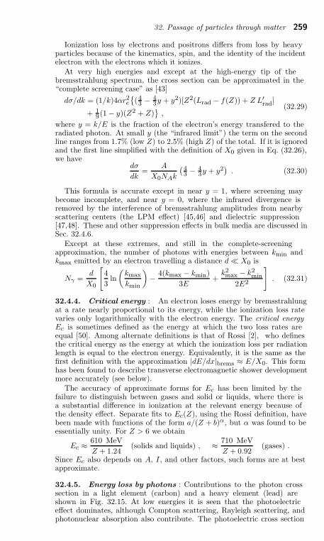
32. Passage of particles through matter 259
Ionization loss by electrons and positrons differs from loss by heavyparticles because of the kinematics, spin, and the identity of the incidentelectron with the electrons which it ionizes.
At very high energies and except at the high-energy tip of thebremsstrahlung spectrum, the cross section can be approximated in the“complete screening case” as [43]
dσ/dk = (1/k)4αr2e
(43 − 4
3y + y2)[Z2(Lrad − f(Z)) + Z L′rad]
+ 19 (1 − y)(Z2 + Z)
,(32.29)
where y = k/E is the fraction of the electron’s energy transfered to theradiated photon. At small y (the “infrared limit”) the term on the secondline ranges from 1.7% (low Z) to 2.5% (high Z) of the total. If it is ignoredand the first line simplified with the definition of X0 given in Eq. (32.26),we have
dσ
dk=
A
X0NAk
(
43 − 4
3y + y2)
. (32.30)
This formula is accurate except in near y = 1, where screening maybecome incomplete, and near y = 0, where the infrared divergence isremoved by the interference of bremsstrahlung amplitudes from nearbyscattering centers (the LPM effect) [45,46] and dielectric suppression[47,48]. These and other suppression effects in bulk media are discussed inSec. 32.4.6.
Except at these extremes, and still in the complete-screeningapproximation, the number of photons with energies between kmin andkmax emitted by an electron travelling a distance d ≪ X0 is
Nγ =d
X0
[
4
3ln
(
kmax
kmin
)
− 4(kmax − kmin)
3E+
k2max − k2
min
2E2
]
. (32.31)
32.4.4. Critical energy : An electron loses energy by bremsstrahlungat a rate nearly proportional to its energy, while the ionization loss ratevaries only logarithmically with the electron energy. The critical energyEc is sometimes defined as the energy at which the two loss rates areequal [50]. Among alternate definitions is that of Rossi [2], who definesthe critical energy as the energy at which the ionization loss per radiationlength is equal to the electron energy. Equivalently, it is the same as thefirst definition with the approximation |dE/dx|brems ≈ E/X0. This formhas been found to describe transverse electromagnetic shower developmentmore accurately (see below).
The accuracy of approximate forms for Ec has been limited by thefailure to distinguish between gases and solid or liquids, where there isa substantial difference in ionization at the relevant energy because ofthe density effect. Separate fits to Ec(Z), using the Rossi definition, havebeen made with functions of the form a/(Z + b)α, but α was found to beessentially unity. For Z > 6 we obtain
Ec ≈ 610 MeV
Z + 1.24(solids and liquids) , ≈ 710 MeV
Z + 0.92(gases) .
Since Ec also depends on A, I, and other factors, such forms are at bestapproximate.
32.4.5. Energy loss by photons : Contributions to the photon crosssection in a light element (carbon) and a heavy element (lead) areshown in Fig. 32.15. At low energies it is seen that the photoelectriceffect dominates, although Compton scattering, Rayleigh scattering, andphotonuclear absorption also contribute. The photoelectric cross section
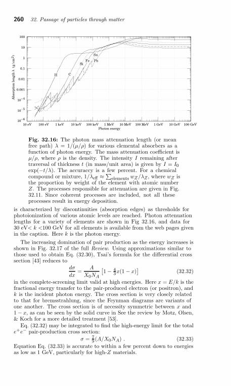
260 32. Passage of particles through matter
Photon energy
100
10
10–4
10–5
10–6
1
0.1
0.01
0.001
10 eV 100 eV 1 keV 10 keV 100 keV 1 MeV 10 MeV 100 MeV 1 GeV 10 GeV 100 GeV
Ab
sorp
tion
len
gth
λ (g/
cm2
)
Si
C
Fe Pb
H
Sn
Fig. 32.16: The photon mass attenuation length (or meanfree path) λ = 1/(µ/ρ) for various elemental absorbers as afunction of photon energy. The mass attenuation coefficient isµ/ρ, where ρ is the density. The intensity I remaining aftertraversal of thickness t (in mass/unit area) is given by I = I0exp(−t/λ). The accuraccy is a few percent. For a chemicalcompound or mixture, 1/λeff ≈
∑
elements wZ/λZ , where wZ isthe proportion by weight of the element with atomic numberZ. The processes responsible for attenuation are given in Fig.32.11. Since coherent processes are included, not all theseprocesses result in energy deposition.
is characterized by discontinuities (absorption edges) as thresholds forphotoionization of various atomic levels are reached. Photon attenuationlengths for a variety of elements are shown in Fig 32.16, and data for30 eV< k <100 GeV for all elements is available from the web pages givenin the caption. Here k is the photon energy.
The increasing domination of pair production as the energy increases isshown in Fig. 32.17 of the full Review. Using approximations similar tothose used to obtain Eq. (32.30), Tsai’s formula for the differential crosssection [43] reduces to
dσ
dx=
A
X0NA
[
1 − 43x(1 − x)
]
(32.32)
in the complete-screening limit valid at high energies. Here x = E/k is thefractional energy transfer to the pair-produced electron (or positron), andk is the incident photon energy. The cross section is very closely relatedto that for bremsstrahlung, since the Feynman diagrams are variants ofone another. The cross section is of necessity symmetric between x and1 − x, as can be seen by the solid curve in See the review by Motz, Olsen,& Koch for a more detailed treatment [53].
Eq. (32.32) may be integrated to find the high-energy limit for the totale+e− pair-production cross section:
σ = 79 (A/X0NA) . (32.33)
Equation Eq. (32.33) is accurate to within a few percent down to energiesas low as 1 GeV, particularly for high-Z materials.
32. Passage of particles through matter 261
32.4.6. Bremsstrahlung and pair production at very high ener-gies : At ultrahigh energies, Eqns. 32.29–32.33 will fail because ofquantum mechanical interference between amplitudes from different scat-tering centers. Since the longitudinal momentum transfer to a given centeris small (∝ k/E(E − k), in the case of bremsstrahlung), the interactionis spread over a comparatively long distance called the formation length(∝ E(E − k)/k) via the uncertainty principle. In alternate language, theformation length is the distance over which the highly relativistic electronand the photon “split apart.” The interference is usually destructive.Calculations of the “Landau-Pomeranchuk-Migdal” (LPM) effect may bemade semi-classically based on the average multiple scattering, or morerigorously using a quantum transport approach [45,46].
In amorphous media, bremsstrahlung is suppressed if the photon energyk is less than E2/(E + ELPM ) [46], where*
ELPM =(mec
2)2αX0
4π~cρ= (7.7 TeV/cm) × X0
ρ. (32.34)
Since physical distances are involved, X0/ρ, in cm, appears. The energy-weighted bremsstrahlung spectrum for lead, k dσLPM/dk, is shown inFig. 27.11 of the full Review. With appropriate scaling by X0/ρ, othermaterials behave similarly.
For photons, pair production is reduced for E(k − E) > k ELPM . Thepair-production cross sections for different photon energies are shown inFig. 32.18 of the full Review.
If k ≪ E, several additional mechanisms can also produce suppression.When the formation length is long, even weak factors can perturbthe interaction. For example, the emitted photon can coherentlyforward scatter off of the electrons in the media. Because of this,for k < ωpE/me ∼ 10−4, bremsstrahlung is suppressed by a factor
(kme/ωpE)2 [48]. Magnetic fields can also suppress bremsstrahlung.In crystalline media, the situation is more complicated, with coherentenhancement or suppression possible [55].
32.5. Electromagnetic cascades
When a high-energy electron or photon is incident on a thick absorber, itinitiates an electromagnetic cascade as pair production and bremsstrahlunggenerate more electrons and photons with lower energy. The longitudinaldevelopment is governed by the high-energy part of the cascade, andtherefore scales as the radiation length in the material. Electron energieseventually fall below the critical energy, and then dissipate their energyby ionization and excitation rather than by the generation of more showerparticles. In describing shower behavior, it is therefore convenient tointroduce the scale variables t = x/X0 and y = E/Ec, so that distanceis measured in units of radiation length and energy in units of criticalenergy.
The mean longitudinal profile of the energy deposition in anelectromagnetic cascade is reasonably well described by a gammadistribution [60]:
dE
dt= E0 b
(bt)a−1e−bt
Γ(a)(32.36)
The maximum tmax occurs at (a − 1)/b. We have made fits to showerprofiles in elements ranging from carbon to uranium, at energies from 1
* This definition differs from that of Ref. 54 by a factor of two. ELPMscales as the 4th power of the mass of the incident particle, so that ELPM =(1.4 × 10¹⁰ TeV/cm) × X0/ρ for a muon.
262 32. Passage of particles through matter
GeV to 100 GeV. The energy deposition profiles are well described byEq. (32.36) with
tmax = (a − 1)/b = 1.0 × (ln y + Cj) , j = e, γ , (32.37)
where Ce = −0.5 for electron-induced cascades and Cγ = +0.5 forphoton-induced cascades. To use Eq. (32.36), one finds (a − 1)/b fromEq. (32.37), then finds a either by assuming b ≈ 0.5 or by finding amore accurate value from Fig. 32.21. The results are very similar for theelectron number profiles, but there is some dependence on the atomicnumber of the medium. A similar form for the electron number maximumwas obtained by Rossi in the context of his “Approximation B,” [2] butwith Ce = −1.0 and Cγ = −0.5; we regard this as superseded by the EGS4result.
The “shower length” Xs = X0/b is less conveniently parameterized,since b depends upon both Z and incident energy, as shown in Fig. 32.21.As a corollary of this Z dependence, the number of electrons crossing aplane near shower maximum is underestimated using Rossi’s approxima-tion for carbon and seriously overestimated for uranium. Essentially thesame b values are obtained for incident electrons and photons. For manypurposes it is sufficient to take b ≈ 0.5.
The gamma function distribution is very flat near the origin, whilethe EGS4 cascade (or a real cascade) increases more rapidly. As a resultEq. (32.36) fails badly for about the first two radiation lengths, which areexcluded from fits. Because fluctuations are important, Eq. (32.36) shouldbe used only in applications where average behavior is adequate.
The transverse development of electromagnetic showers in differentmaterials scales fairly accurately with the Moliere radius RM , given by[62,63]
RM = X0 Es/Ec , (32.38)
where Es ≈ 21 MeV (Table 32.1), and the Rossi definition of Ec is used.Measurements of the lateral distribution in electromagnetic cascades
are shown in Ref. 62 and 63. On the average, only 10% of the energylies outside the cylinder with radius RM . About 99% is containedinside of 3.5RM , but at this radius and beyond composition effectsbecome important and the scaling with RM fails. The distributions arecharacterized by a narrow core, and broaden as the shower develops. Theyare often represented as the sum of two Gaussians, and Grindhammer [61]describes them with the function
f(r) =2r R2
(r2 + R2)2, (32.40)
where R is a phenomenological function of x/X0 and lnE.
At high enough energies, the LPM effect (Sec. 32.4.6) reduces the crosssections for bremsstrahlung and pair production, and hence can causesignificant elongation of electromagnetic cascades [56].
32.6. Muon energy loss at high energy
At sufficiently high energies, radiative processes become more importantthan ionization for all charged particles. For muons and pions in materialssuch as iron, this “critical energy” occurs at several hundred GeV. (Thereis no simple scaling with particle mass, but for protons the “criticalenergy” is much, much higher.) Radiative effects dominate the energyloss of energetic muons found in cosmic rays or produced at the newestaccelerators. These processes are characterized by small cross sections,hard spectra, large energy fluctuations, and the associated generation ofelectromagnetic and (in the case of photonuclear interactions) hadronic
32. Passage of particles through matter 263
showers [61–69]. At these energies the treatment of energy loss as auniform and continuous process is for many purposes inadequate.
It is convenient to write the average rate of muon energy loss as [73]
−dE/dx = a(E) + b(E)E . (32.41)
Here a(E) is the ionization energy loss given by Eq. (32.5), and b(E)is the sum of e+e− pair production, bremsstrahlung, and photonuclearcontributions. To the approximation that these slowly-varying functionsare constant, the mean range x0 of a muon with initial energy E0 is givenby
x0 ≈ (1/b) ln(1 + E0/Eµc) , (32.42)
where Eµc = a/b.
The “muon critical energy” Eµc can be defined more exactly as theenergy at which radiative and ionization losses are equal, and can befound by solving Eµc = a(Eµc)/b(Eµc). This definition corresponds to thesolid-line intersection in 32.13 of the full Review, and is different from theRossi definition we used for electrons. It serves the same function: belowEµc ionization losses dominate, and above Eµc radiative effects dominate.The dependence of Eµc on atomic number Z is shown in Fig. 32.24 in thefull Review.
The radiative cross sections are expressed as functions of the fractionalenergy loss ν. The bremsstrahlung cross section goes roughly as 1/ν overmost of the range, while for the pair production case the distributiongoes as ν−3 to ν−2 [74]. “Hard” losses are therefore more probable inbremsstrahlung, and in fact energy losses due to pair production mayvery nearly be treated as continuous. The simulated [72] momentumdistribution of an incident 1 TeV/c muon beam after it crosses 3 m ofiron is shown in Fig. 32.25 of the full Review. The hard bremsstrahlungphotons and hadronic debris from photonuclear interactions inducecascades which can obscure muon tracks in detector planes and reducetracking [76].
32.7. Cherenkov and transitional radiation[33,77,78]
A charged particle radiates if its velocity is greater than the local phasevelocity of light (Cherenkov radiation) or if it crosses suddenly from onemedium to another with different optical properties (transition radiation).Neither process is important for energy loss, but both are used inhigh-energy physics detectors.
32.7.1. Optical Cherenkov radiation : The cosine of the angle θc ofCherenkov radiation, relative to the particle’s direction, for a particle withvelocity βc in a medium with index of refraction n, is 1/nβ, or
tan θc =√
β2n2 − 1 ≈√
2(1 − 1/nβ) (32.43)
for small θc, e.g., in gases. The threshold velocity βt is 1/n, and
γt = 1/(1 − β2t )1/2. Therefore, βtγt = 1/(2δ + δ2)1/2, where δ = n − 1.
Practical Cherenkov radiator materials are dispersive. Let ω be thephoton’s frequency, and let k = 2π/λ be its wavenumber. The photonspropage at the group velocity vg = dω/dk = c/[n(ω) + ω(dn/dω)]. In anon-dispersive medium, this simplifies to vg = c/n.
The number of photons produced per unit path length of a particlewith charge ze and per unit energy interval of the photons is
d2N
dEdx=
αz2
~csin2 θc =
α2z2
re mec2
(
1 − 1
β2n2(E)
)
≈ 370 sin2 θc(E) eV−1cm−1 (z = 1) , (32.45)
264 32. Passage of particles through matter
or, equivalently,
d2N
dxdλ=
2παz2
λ2
(
1 − 1
β2n2(λ)
)
. (32.46)
The index of refraction n is a function of photon energy E = ~ω. Forpractical use, Eq. (32.45) must be multiplied by the photodetector responsefunction and integrated over the region for which β n(ω) > 1.
When two particles are within <∼ 1 wavelength, the electromagneticfields from the particles may add coherently, affecting the Cherenkovradiation. The radiation from an e+e− pair at close separation issuppressed compared to two independent leptons [84].
32.7.2. Coherent radio Cherenkov radiation :Coherent Cherenkov radiation is produced by many charged particles
with a non-zero net charge moving through matter on an approximatelycommon “wavefront”—for example, the electrons and positrons in ahigh-energy electromagnetic cascade. The signals can be visible abovebackgrounds for shower energies as low as 1017 eV; see Sec. 34.3.3 for moredetails. The phenomenon is called the Askaryan effect [85]. The photonscan Compton-scatter atomic electrons, and positrons can annihilate withatomic electrons to contribute even more photons which can in turnCompton scatter. These processes result in a roughly 20% excess ofelectrons over positrons in a shower. The net negative charge leads tocoherent radio Cherenkov emission. Because the emission is coherent, theelectric field strength is proportional to the shower energy, and the signalpower increases as its square. The electric field strength also increaseslinearly with frequency, up to a maximum frequency determined by thelateral spread of the shower. This cutoff occurs at about 1 GHz in ice, andscales inversely with the Moliere radius. At low frequencies, the radiationis roughly isotropic, but, as the frequency rises toward the cutoff frequency,the radiation becomes increasingly peaked around the Cherenkov angle.
32.7.3. Transition radiation : The energy I radiated when a particlewith charge ze crosses the boundary between vacuum and a medium withplasma frequency ωp is αz2γ~ωp/3, where
~ωp =√
4πNer3e mec
2/α =
√
ρ (in g/cm3) 〈Z/A〉 × 28.81 eV . (32.48)
For styrene and similar materials, ~ωp ≈ 20 eV; for air it is 0.7 eV.The number spectrum dNγ/d(~ω diverges logarithmically at low
energies and decreases rapidly for ~ω/γ~ωp > 1. About half the energyis emitted in the range 0.1 ≤ ~ω/γ~ωp ≤ 1. Inevitable absorption in a
practical detector removes the divergence. For a particle with γ = 103,the radiated photons are in the soft x-ray range 2 to 40 keV. The γdependence of the emitted energy thus comes from the hardening of thespectrum rather than from an increased quantum yield.
The number of photons with energy ~ω > ~ω0 is given by the answerto problem 13.15 in Ref. 33,
Nγ(~ω > ~ω0) =αz2
π
[
(
lnγ~ωp
~ω0− 1
)2
+π2
12
]
, (32.49)
within corrections of order (~ω0/γ~ωp)2. The number of photons above a
fixed energy ~ω0 ≪ γ~ωp thus grows as (ln γ)2, but the number above afixed fraction of γ~ωp (as in the example above) is constant. For example,
for ~ω > γ~ωp/10, Nγ = 2.519 αz2/π = 0.59%× z2.The particle stays “in phase” with the x ray over a distance called the
formation length, d(ω). Most of the radiation is produced in a distance
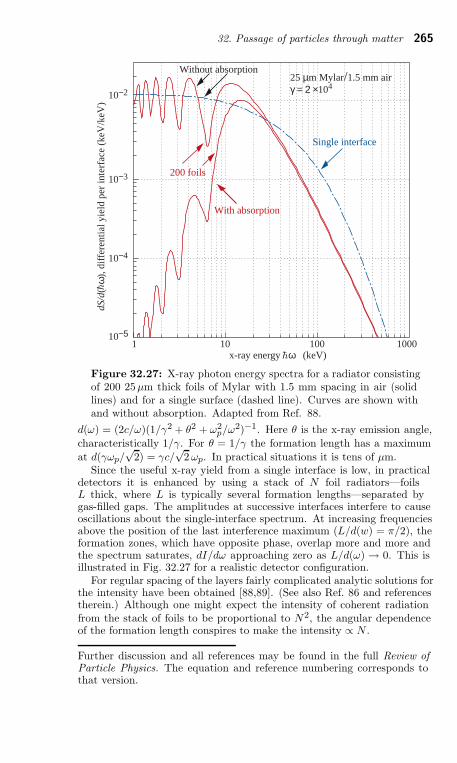
32. Passage of particles through matter 265
10−3
10−2
10−4
10−5101 100 1000
25 µm Mylar/1.5 mm airγ = 2 ×10⁴
Without absorption
With absorption
200 foils
Single interface
x-ray energy ω (keV)
dS/d
( ω
), d
iffe
rent
ial y
ield
per
inte
rfac
e (k
eV/k
eV)
Figure 32.27: X-ray photon energy spectra for a radiator consistingof 200 25µm thick foils of Mylar with 1.5 mm spacing in air (solidlines) and for a single surface (dashed line). Curves are shown withand without absorption. Adapted from Ref. 88.
d(ω) = (2c/ω)(1/γ2 + θ2 + ω2p/ω2)−1. Here θ is the x-ray emission angle,
characteristically 1/γ. For θ = 1/γ the formation length has a maximum
at d(γωp/√
2) = γc/√
2 ωp. In practical situations it is tens of µm.Since the useful x-ray yield from a single interface is low, in practical
detectors it is enhanced by using a stack of N foil radiators—foilsL thick, where L is typically several formation lengths—separated bygas-filled gaps. The amplitudes at successive interfaces interfere to causeoscillations about the single-interface spectrum. At increasing frequenciesabove the position of the last interference maximum (L/d(w) = π/2), theformation zones, which have opposite phase, overlap more and more andthe spectrum saturates, dI/dω approaching zero as L/d(ω) → 0. This isillustrated in Fig. 32.27 for a realistic detector configuration.
For regular spacing of the layers fairly complicated analytic solutions forthe intensity have been obtained [88,89]. (See also Ref. 86 and referencestherein.) Although one might expect the intensity of coherent radiationfrom the stack of foils to be proportional to N2, the angular dependenceof the formation length conspires to make the intensity ∝ N .
Further discussion and all references may be found in the full Review ofParticle Physics. The equation and reference numbering corresponds tothat version.
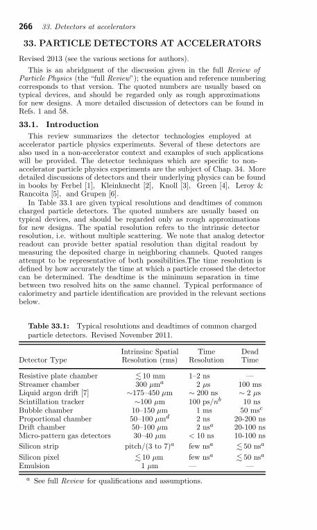
266 33. Detectors at accelerators
33. PARTICLE DETECTORS AT ACCELERATORS
Revised 2013 (see the various sections for authors).
This is an abridgment of the discussion given in the full Review ofParticle Physics (the “full Review”); the equation and reference numberingcorresponds to that version. The quoted numbers are usually based ontypical devices, and should be regarded only as rough approximationsfor new designs. A more detailed discussion of detectors can be found inRefs. 1 and 58.
33.1. Introduction
This review summarizes the detector technologies employed ataccelerator particle physics experiments. Several of these detectors arealso used in a non-accelerator context and examples of such applicationswill be provided. The detector techniques which are specific to non-accelerator particle physics experiments are the subject of Chap. 34. Moredetailed discussions of detectors and their underlying physics can be foundin books by Ferbel [1], Kleinknecht [2], Knoll [3], Green [4], Leroy &Rancoita [5], and Grupen [6].
In Table 33.1 are given typical resolutions and deadtimes of commoncharged particle detectors. The quoted numbers are usually based ontypical devices, and should be regarded only as rough approximationsfor new designs. The spatial resolution refers to the intrinsic detectorresolution, i.e. without multiple scattering. We note that analog detectorreadout can provide better spatial resolution than digital readout bymeasuring the deposited charge in neighboring channels. Quoted rangesattempt to be representative of both possibilities.The time resolution isdefined by how accurately the time at which a particle crossed the detectorcan be determined. The deadtime is the minimum separation in timebetween two resolved hits on the same channel. Typical performance ofcalorimetry and particle identification are provided in the relevant sectionsbelow.
Table 33.1: Typical resolutions and deadtimes of common chargedparticle detectors. Revised November 2011.
Intrinsinc Spatial Time DeadDetector Type Resolution (rms) Resolution Time
Resistive plate chamber . 10 mm 1–2 ns —Streamer chamber 300 µma 2 µs 100 msLiquid argon drift [7] ∼175–450 µm ∼ 200 ns ∼ 2 µsScintillation tracker ∼100 µm 100 ps/nb 10 nsBubble chamber 10–150 µm 1 ms 50 msc
Proportional chamber 50–100 µmd 2 ns 20-200 nsDrift chamber 50–100 µm 2 nsa 20-100 nsMicro-pattern gas detectors 30–40 µm < 10 ns 10-100 ns
Silicon strip pitch/(3 to 7)a few nsa . 50 nsa
Silicon pixel . 10 µm few nsa . 50 nsa
Emulsion 1 µm — —
a See full Review for qualifications and assumptions.
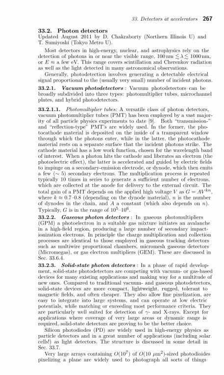
33. Detectors at accelerators 267
33.2. Photon detectorsUpdated August 2011 by D. Chakraborty (Northern Illinois U) andT. Sumiyoshi (Tokyo Metro U).
Most detectors in high-energy, nuclear, and astrophysics rely on thedetection of photons in or near the visible range, 100 nm .λ . 1000nm,or E ≈ a few eV. This range covers scintillation and Cherenkov radiationas well as the light detected in many astronomical observations.
Generally, photodetection involves generating a detectable electricalsignal proportional to the (usually very small) number of incident photons.
33.2.1. Vacuum photodetectors : Vacuum photodetectors can bebroadly subdivided into three types: photomultiplier tubes, microchannelplates, and hybrid photodetectors.
33.2.1.1. Photomultiplier tubes: A versatile class of photon detectors,vacuum photomultiplier tubes (PMT) has been employed by a vast major-ity of all particle physics experiments to date [9]. Both “transmission-”and “reflection-type” PMT’s are widely used. In the former, the pho-tocathode material is deposited on the inside of a transparent windowthrough which the photons enter, while in the latter, the photocathodematerial rests on a separate surface that the incident photons strike. Thecathode material has a low work function, chosen for the wavelength bandof interest. When a photon hits the cathode and liberates an electron (thephotoelectric effect), the latter is accelerated and guided by electric fieldsto impinge on a secondary-emission electrode, or dynode, which then emitsa few (∼ 5) secondary electrons. The multiplication process is repeatedtypically 10 times in series to generate a sufficient number of electrons,which are collected at the anode for delivery to the external circuit. Thetotal gain of a PMT depends on the applied high voltage V as G = AV kn,where k ≈ 0.7–0.8 (depending on the dynode material), n is the numberof dynodes in the chain, and A a constant (which also depends on n).Typically, G is in the range of 105–106.
33.2.2. Gaseous photon detectors : In gaseous photomultipliers(GPM) a photoelectron in a suitable gas mixture initiates an avalanchein a high-field region, producing a large number of secondary impact-ionization electrons. In principle the charge multiplication and collectionprocesses are identical to those employed in gaseous tracking detectorssuch as multiwire proportional chambers, micromesh gaseous detectors(Micromegas), or gas electron multipliers (GEM). These are discussed inSec. 33.6.4.
33.2.3. Solid-state photon detectors : In a phase of rapid develop-ment, solid-state photodetectors are competing with vacuum- or gas-baseddevices for many existing applications and making way for a multitude ofnew ones. Compared to traditional vacuum- and gaseous photodetectors,solid-state devices are more compact, lightweight, rugged, tolerant tomagnetic fields, and often cheaper. They also allow fine pixelization, areeasy to integrate into large systems, and can operate at low electricpotentials, while matching or exceeding most performance criteria. Theyare particularly well suited for detection of γ- and X-rays. Except forapplications where coverage of very large areas or dynamic range isrequired, solid-state detectors are proving to be the better choice.
Silicon photodiodes (PD) are widely used in high-energy physics asparticle detectors and in a great number of applications (including solarcells!) as light detectors. The structure is discussed in some detail inSec. 33.7.
Very large arrays containing O(107) of O(10 µm2)-sized photodioidespixelizing a plane are widely used to photograph all sorts of things
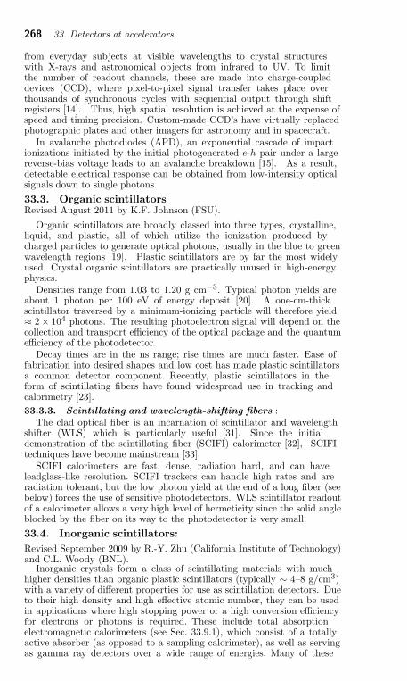
268 33. Detectors at accelerators
from everyday subjects at visible wavelengths to crystal structureswith X-rays and astronomical objects from infrared to UV. To limitthe number of readout channels, these are made into charge-coupleddevices (CCD), where pixel-to-pixel signal transfer takes place overthousands of synchronous cycles with sequential output through shiftregisters [14]. Thus, high spatial resolution is achieved at the expense ofspeed and timing precision. Custom-made CCD’s have virtually replacedphotographic plates and other imagers for astronomy and in spacecraft.
In avalanche photodiodes (APD), an exponential cascade of impactionizations initiated by the initial photogenerated e-h pair under a largereverse-bias voltage leads to an avalanche breakdown [15]. As a result,detectable electrical response can be obtained from low-intensity opticalsignals down to single photons.
33.3. Organic scintillatorsRevised August 2011 by K.F. Johnson (FSU).
Organic scintillators are broadly classed into three types, crystalline,liquid, and plastic, all of which utilize the ionization produced bycharged particles to generate optical photons, usually in the blue to greenwavelength regions [19]. Plastic scintillators are by far the most widelyused. Crystal organic scintillators are practically unused in high-energyphysics.
Densities range from 1.03 to 1.20 g cm−3. Typical photon yields areabout 1 photon per 100 eV of energy deposit [20]. A one-cm-thickscintillator traversed by a minimum-ionizing particle will therefore yield≈ 2 × 10⁴ photons. The resulting photoelectron signal will depend on thecollection and transport efficiency of the optical package and the quantumefficiency of the photodetector.
Decay times are in the ns range; rise times are much faster. Ease offabrication into desired shapes and low cost has made plastic scintillatorsa common detector component. Recently, plastic scintillators in theform of scintillating fibers have found widespread use in tracking andcalorimetry [23].
33.3.3. Scintillating and wavelength-shifting fibers :The clad optical fiber is an incarnation of scintillator and wavelength
shifter (WLS) which is particularly useful [31]. Since the initialdemonstration of the scintillating fiber (SCIFI) calorimeter [32], SCIFItechniques have become mainstream [33].
SCIFI calorimeters are fast, dense, radiation hard, and can haveleadglass-like resolution. SCIFI trackers can handle high rates and areradiation tolerant, but the low photon yield at the end of a long fiber (seebelow) forces the use of sensitive photodetectors. WLS scintillator readoutof a calorimeter allows a very high level of hermeticity since the solid angleblocked by the fiber on its way to the photodetector is very small.
33.4. Inorganic scintillators:
Revised September 2009 by R.-Y. Zhu (California Institute of Technology)and C.L. Woody (BNL).
Inorganic crystals form a class of scintillating materials with muchhigher densities than organic plastic scintillators (typically ∼ 4–8 g/cm3)with a variety of different properties for use as scintillation detectors. Dueto their high density and high effective atomic number, they can be usedin applications where high stopping power or a high conversion efficiencyfor electrons or photons is required. These include total absorptionelectromagnetic calorimeters (see Sec. 33.9.1), which consist of a totallyactive absorber (as opposed to a sampling calorimeter), as well as servingas gamma ray detectors over a wide range of energies. Many of these
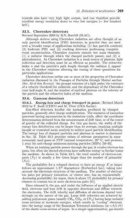
33. Detectors at accelerators 269
crystals also have very high light output, and can therefore provideexcellent energy resolution down to very low energies (∼ few hundredkeV).
33.5. Cherenkov detectorsRevised September 2009 by B.N. Ratcliff (SLAC).
Although devices using Cherenkov radiation are often thought of asonly particle identification (PID) detectors, in practice they are usedover a broader range of applications including; (1) fast particle counters;(2) hadronic PID; and (3) tracking detectors performing completeevent reconstruction. Cherenkov counters contain two main elements;(1) a radiator through which the charged particle passes, and (2) aphotodetector. As Cherenkov radiation is a weak source of photons, lightcollection and detection must be as efficient as possible. The refractiveindex n and the particle’s path length through the radiator L appearin the Cherenkov relations allowing the tuning of these quantities forparticular applications.
Cherenkov detectors utilize one or more of the properties of Cherenkovradiation discussed in the Passages of Particles through Matter section(Sec. 32 of this Review): the prompt emission of a light pulse; the existenceof a velocity threshold for radiation; and the dependence of the Cherenkovcone half-angle θc and the number of emitted photons on the velocity ofthe particle and the refractive index of the medium.
33.6. Gaseous detectors
33.6.1. Energy loss and charge transport in gases : Revised March2010 by F. Sauli (CERN) and M. Titov (CEA Saclay).
Gas-filled detectors localize the ionization produced by chargedparticles, generally after charge multiplication. The statistics of ionizationprocesses having asymmetries in the ionization trails, affect the coordinatedetermination deduced from the measurement of drift time, or of the centerof gravity of the collected charge. For thin gas layers, the width of theenergy loss distribution can be larger than its average, requiring multiplesample or truncated mean analysis to achieve good particle identification.The energy loss of charged particles and photons in matter is discussedin Sec. 32. Table 33.5 provides values of relevant parameters in somecommonly used gases at NTP (normal temperature, 20 C, and pressure,1 atm) for unit-charge minimum-ionizing particles (MIPs) [59–65].
When an ionizing particle passes through the gas, it creates electron-ionpairs, but often the ejected electrons have sufficient energy to further ionizethe medium. As shown in Table 33.5, the total number of electron-ionpairs (NT ) is usually a few times larger than the number of primaries(NP ).
The probability for a released electron to have an energy E or largerfollows an approximate 1/E2 dependence (Rutherford law), taking intoaccount the electronic structure of the medium. The number of electron-ion pairs per primary ionization, or cluster size, has an exponentiallydecreasing probability; for argon, there is about 1% probability for primaryclusters to contain ten or more electron-ion pairs [61].
Once released in the gas, and under the influence of an applied electricfield, electrons and ions drift in opposite directions and diffuse towardsthe electrodes. The drift velocity and diffusion of electrons depend verystrongly on the nature of the gas. Large drift velocities are achieved byadding polyatomic gases (usually CH4, CO2, or CF4) having large inelasticcross sections at moderate energies, which results in “cooling” electronsinto the energy range of the Ramsauer-Townsend minimum (at ∼ 0.5 eV)of the elastic cross-section of argon. In a simple approximation, gas kinetic
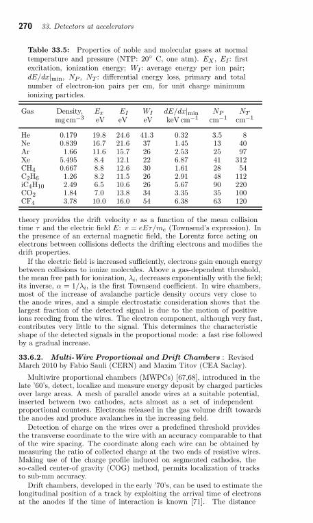
270 33. Detectors at accelerators
Table 33.5: Properties of noble and molecular gases at normaltemperature and pressure (NTP: 20 C, one atm). EX , EI : firstexcitation, ionization energy; WI : average energy per ion pair;dE/dx|min, NP , NT : differential energy loss, primary and totalnumber of electron-ion pairs per cm, for unit charge minimumionizing particles.
Gas Density, Ex EI WI dE/dx|min NP NTmgcm−3 eV eV eV keV cm−1 cm−1 cm−1
He 0.179 19.8 24.6 41.3 0.32 3.5 8Ne 0.839 16.7 21.6 37 1.45 13 40Ar 1.66 11.6 15.7 26 2.53 25 97Xe 5.495 8.4 12.1 22 6.87 41 312CH4 0.667 8.8 12.6 30 1.61 28 54C2H6 1.26 8.2 11.5 26 2.91 48 112iC4H10 2.49 6.5 10.6 26 5.67 90 220CO2 1.84 7.0 13.8 34 3.35 35 100CF4 3.78 10.0 16.0 54 6.38 63 120
theory provides the drift velocity v as a function of the mean collisiontime τ and the electric field E: v = eEτ/me (Townsend’s expression). Inthe presence of an external magnetic field, the Lorentz force acting onelectrons between collisions deflects the drifting electrons and modifies thedrift properties.
If the electric field is increased sufficiently, electrons gain enough energybetween collisions to ionize molecules. Above a gas-dependent threshold,the mean free path for ionization, λi, decreases exponentially with the field;its inverse, α = 1/λi, is the first Townsend coefficient. In wire chambers,most of the increase of avalanche particle density occurs very close tothe anode wires, and a simple electrostatic consideration shows that thelargest fraction of the detected signal is due to the motion of positiveions receding from the wires. The electron component, although very fast,contributes very little to the signal. This determines the characteristicshape of the detected signals in the proportional mode: a fast rise followedby a gradual increase.
33.6.2. Multi-Wire Proportional and Drift Chambers : RevisedMarch 2010 by Fabio Sauli (CERN) and Maxim Titov (CEA Saclay).
Multiwire proportional chambers (MWPCs) [67,68], introduced in thelate ’60’s, detect, localize and measure energy deposit by charged particlesover large areas. A mesh of parallel anode wires at a suitable potential,inserted between two cathodes, acts almost as a set of independentproportional counters. Electrons released in the gas volume drift towardsthe anodes and produce avalanches in the increasing field.
Detection of charge on the wires over a predefined threshold providesthe transverse coordinate to the wire with an accuracy comparable to thatof the wire spacing. The coordinate along each wire can be obtained bymeasuring the ratio of collected charge at the two ends of resistive wires.Making use of the charge profile induced on segmented cathodes, theso-called center-of gravity (COG) method, permits localization of tracksto sub-mm accuracy.
Drift chambers, developed in the early ’70’s, can be used to estimate thelongitudinal position of a track by exploiting the arrival time of electronsat the anodes if the time of interaction is known [71]. The distance
33. Detectors at accelerators 271
between anode wires is usually several cm, allowing coverage of large areasat reduced cost.
33.6.4. Micro-Pattern Gas Detectors : Revised March 2010 byFabio Sauli (CERN) and Maxim Titov (CEA Saclay).
By using pitch size of a few hundred µm, an order of magnitudeimprovement in granularity over wire chambers, these detectors offerintrinsic high rate capability (> 106 Hz/mm2), excellent spatial res-olution (∼ 30 µm), multi-particle resolution (∼ 500 µm), and singlephoto-electron time resolution in the ns range.
The Gas Electron Multiplier (GEM) detector consists of a thin-foilcopper-insulator-copper sandwich chemically perforated to obtain a highdensity of holes in which avalanches occur [88]. The hole diameter istypically between 25 µm and 150 µm, while the corresponding distancebetween holes varies between 50 µm and 200 µm. The central insulatoris usually (in the original design) the polymer Kapton, with a thicknessof 50 µm. Application of a potential difference between the two sides ofthe GEM generates the electric fields. Each hole acts as an independentproportional counter. Electrons released by the primary ionization particlein the upper conversion region (above the GEM foil) drift into the holes,where charge multiplication occurs in the high electric field (50–70 kV/cm).Most of avalanche electrons are transferred into the gap below the GEM.Several GEM foils can be cascaded, allowing the multi-layer GEMdetectors to operate at overall gas gain above 104 in the presence of highlyionizing particles, while strongly reducing the risk of discharges.
The micro-mesh gaseous structure (Micromegas) is a thin parallel-plateavalanche counter. It consists of a drift region and a narrow multiplicationgap (25–150 µm) between a thin metal grid (micromesh) and the readoutelectrode (strips or pads of conductor printed on an insulator board).Electrons from the primary ionization drift through the holes of the meshinto the narrow multiplication gap, where they are amplified. The smallamplification gap produces a narrow avalanche, giving rise to excellentspatial resolution: 12 µm accuracy, limited by the micro-mesh pitch, hasbeen achieved for MIPs, as well as very good time resolution and energyresolution (∼ 12% FWHM with 6 keV x rays) [91].
The performance and robustness of GEM and Micromegas haveencouraged their use in high-energy and nuclear physics, UV and visiblephoton detection, astroparticle and neutrino physics, neutron detectionand medical physics.
33.6.5. Time-projection chambers : Revised October 2011 by D.Karlen (U. of Victoria and TRIUMF, Canada).
The Time Projection Chamber (TPC) concept, invented by DavidNygren in the late 1970’s [76], is the basis for charged particle trackingin a large number of particle and nuclear physics experiments. A uniformelectric field drifts tracks of electrons produced by charged particlestraversing a medium, either gas or liquid, towards a surface segmented into2D readout pads. The signal amplitudes and arrival times are recorded toprovide full 3D measurements of the particle trajectories. The intrinsic 3Dsegmentation gives the TPC a distinct advantage over other large volumetracking detector designs which record information only in a 2D projectionwith less overall segmentation, particularly for pattern recognition inevents with large numbers of particles.
Gaseous TPC’s are often designed to operate within a strong magneticfield (typically parallel to the drift field) so that particle momenta canbe estimated from the track curvature. For this application, precisespatial measurements in the plane transverse to the magnetic field aremost important. Since the amount of ionization along the length of the
272 33. Detectors at accelerators
track depends on the velocity of the particle, ionization and momentummeasurements can be combined to identify the types of particles observedin the TPC.
Gas amplification of 103–104 at the readout endplate is usually requiredin order to provide signals with sufficient amplitude for conventionalelectronics to sense the drifted ionization. Until recently, the gasamplification system used in TPC’s have exclusively been planes of anodewires operated in proportional mode placed close to the readout pads.Performance has been recently improved by replacing these wire planeswith micro-pattern gas detectors, namely GEM [88] and Micromegas [90]devices.
Diffusion degrades the position information of ionization that drifts along distance. For a gaseous TPC, the effect can be alleviated by thechoice of a gas with low intrinsic diffusion or by operating in a strongmagnetic field parallel to the drift field with a gas which exhibits asignificant reduction in transverse diffusion with magnetic field.
33.6.6. Transition radiation detectors (TRD’s) : Revised August2013 by P. Nevski (BNL) and A. Romaniouk (Moscow Eng. & Phys.Inst.).
Transition radiation (TR) x rays are produced when a highly relativisticparticle (γ >∼ 103) crosses a refractive index interface, as discussed inSec. 32.7. The x rays, ranging from a few keV to a few dozen keV, areemitted at a characteristic angle 1/γ from the particle trajectory. Sincethe TR yield is about 1% per boundary crossing, radiation from multiplesurface crossings is used in practical detectors. In the simplest concept, adetector module might consist of low-Z foils followed by a high-Z activelayer made of proportional counters filled with a Xe-rich gas mixture.The atomic number considerations follow from the dominant photoelectricabsorption cross section per atom going roughly as Z n/E3
x, where n variesbetween 4 and 5 over the region of interest, and the x-ray energy is Ex. Tominimize self-absorption, materials such as polypropylene, Mylar, carbon,and (rarely) lithium are used as radiators. The TR signal in the activeregions is in most cases superimposed upon the particle’s ionization losseswhich are proportional to Z.
The TR intensity for a single boundary crossing always increases withγ, but for multiple boundary crossings interference leads to saturationnear a Lorentz factor γ sat = 0.6 ω1
√ℓ1ℓ2/c [105], where ω1 is the radiator
plasma frequency, ℓ1 is its thickness, and ℓ2 the spacing. In most ofthe detectors used in particle physics the radiator parameters are chosento provide γ sat ≈ 2000. Those detectors normally work as thresholddevices, ensuring the best electron/pion separation in the momentumrange 1 GeV/c <∼ p <∼ 150 GeV/c.
The discrimination between electrons and pions can be based on thecharge deposition measured in each detection module, on the number ofclusters—energy depositions observed above an optimal threshold (usuallyit is 5–7 keV), or on more sophisticated methods analyzing the pulse shapeas a function of time. The total energy measurement technique is moresuitable for thick gas volumes, which absorb most of the TR radiationand where the ionization loss fluctuations are small. The cluster-countingmethod works better for detectors with thin gas layers, where thefluctuations of the ionization losses are big.
Recent TRDs for particle astrophysics are designed to directly measurethe Lorentz factor of high-energy nuclei by using the quadratic dependenceof the TR yield on nuclear charge; see Cherry and Muller papers inRef. 107.
33. Detectors at accelerators 273
33.7. Semiconductor detectorsUpdated November 2013 by H. Spieler (LBNL).
Semiconductor detectors provide a unique combination of energy andposition resolution. In collider detectors they are most widely used asposition sensing devices and photodetectors (Sec. 33.2).
33.7.1. Materials Requirements : Semiconductor detectors are essen-tially solid state ionization chambers. Absorbed energy forms electron-holepairs, i.e., negative and positive charge carriers, which under an appliedelectric field move towards their respective collection electrodes, wherethey induce a signal current. The energy required to form an electron-holepair is proportional to the bandgap. In tracking detectors the energy lossin the detector should be minimal, whereas for energy spectroscopy thestopping power should be maximized, so for gamma rays high-Z materialsare desirable.
Measurements on silicon photodiodes [121] show that for photonenergies below 4 eV one electron-hole (e-h) pair is formed per incidentphoton. The mean energy Ei required to produce an e-h pair peaks at4.4 eV for a photon energy around 6 eV. Above ∼1.5 keV it assumesa constant value, 3.67 eV at room temperature. It is larger than thebandgap energy because momentum conservation requires excitation oflattice vibrations (phonons). For minimum-ionizing particles, the mostprobable charge deposition in a 300 µm thick silicon detector is about3.5 fC (22000 electrons). Other typical ionization energies are 2.96 eV inGe, 4.2 eV in GaAs, and 4.43 eV in CdTe.
Since both electronic and lattice excitations are involved, the variancein the number of charge carriers N = E/Ei produced by an absorbedenergy E is reduced by the Fano factor F (about 0.1 in Si and Ge). Thus,
σN =√
FN and the energy resolution σE/E =√
FEi/E. However, themeasured signal fluctuations are usually dominated by electronic noise orenergy loss fluctuations in the detector.
A major effort is to find high-Z materials with a bandgap that issufficiently high to allow room-temperature operation while still providinggood energy resolution. Compund semiconductors, e.g., CdZnTe, can allowthis, but typically suffer from charge collection problems, characterizedby the product µτ of mobility and carrier lifetime. In Si and Geµτ > 1 cm2 V−1 for both electrons and holes, whereas in compoundsemiconductors it is in the range 10−3–10−8. Since for holes µτ is typicallyan order of magnitude smaller than for electrons, detector configurationswhere the electron contribution to the charge signal dominates—e.g., stripor pixel structures—can provide better performance.
33.7.2. Detector Configurations : A p-n junction operated at reversebias forms a sensitive region depleted of mobile charge and sets up anelectric field that sweeps charge liberated by radiation to the electrodes.Detectors typically use an asymmetric structure, e.g., a highly dopedp electrode and a lightly doped n region, so that the depletion regionextends predominantly into the lightly doped volume.In a planar device the thickness of the depleted region is
W =√
2ǫ (V + Vbi)/Ne =√
2ρµǫ(V + Vbi) , (33.18)
where V = external bias voltageVbi = “built-in” voltage (≈ 0.5 V for resistivities typically used in Si
detectors)N = doping concentratione = electronic chargeǫ = dielectric constant = 11.9 ǫ0 ≈ 1 pF/cm in Si
274 33. Detectors at accelerators
ρ = resistivity (typically 1–10 kΩ cm in Si)
µ = charge carrier mobility
= 1350 cm2 V−1 s−1 for electrons in Si
= 450 cm2 V−1 s−1 for holes in SiIn SiW = 0.5 [µm/
√Ω-cm · V] ×
√
ρ(V + Vbi) for n-type Si, and
W = 0.3 [µm/√
Ω-cm · V] ×√
ρ(V + Vbi) for p-type Si.
Large volume (∼ 102–103 cm3) Ge detectors are commonly configured ascoaxial detectors, e.g., a cylindrical n-type crystal with 5–10 cm diameterand 10 cm length with an inner 5–10mm diameter n+ electrode and anouter p+ layer forming the diode junction. Ge can be grown with verylow impurity levels, 109–1010 cm−3 (HPGe), so these large volumes can bedepleted with several kV.
33.7.3. Signal Formation : The signal pulse shape depends on theinstantaneous carrier velocity v(x) = µE(x) and the electrode geometry,which determines the distribution of induced charge (e.g., see Ref. 120,pp. 71–83). Charge collection time decreases with increasing bias voltage,and can be reduced further by operating the detector with “overbias,”i.e., a bias voltage exceeding the value required to fully deplete the device.The collection time is limited by velocity saturation at high fields (in Siapproaching 107 cm/s at E > 104 V/cm); at an average field of 104 V/cmthe collection time is about 15 ps/µm for electrons and 30 ps/µm for holes.In typical fully-depleted detectors 300 µm thick, electrons are collectedwithin about 10 ns, and holes within about 25 ns.
Position resolution is limited by transverse diffusion during chargecollection (typically 5 µm for 300 µm thickness) and by knock-on electrons.Resolutions of 2–4 µm (rms) have been obtained in beam tests. Inmagnetic fields, the Lorentz drift deflects the electron and hole trajectoriesand the detector must be tilted to reduce spatial spreading (see “Halleffect” in semiconductor textbooks).
Electrodes can be in the form of cm-scale pads, strips, or µm-scalepixels. Various readout structures have been developed for pixels, e.g.,CCDs, DEPFETs, monolithic pixel devices that integrate sensor andelectronics (MAPS), and hybrid pixel devices that utilize separate sensorsand readout ICs connected by two-dimensional arrays of solder bumps.For an overview and further discussion see Ref. 120.
33.7.4. Radiation Damage : Radiation damage occurs through twobasic mechanisms:
1. Bulk damage due to displacement of atoms from their latticesites. This leads to increased leakage current, carrier trapping, andbuild-up of space charge that changes the required operating voltage.Displacement damage depends on the nonionizing energy loss andthe energy imparted to the recoil atoms, which can initiate a chain ofsubsequent displacements, i.e., damage clusters. Hence, it is criticalto consider both particle type and energy.
2. Surface damage due to charge build-up in surface layers, which leadsto increased surface leakage currents. In strip detectors the inter-stripisolation is affected. The effects of charge build-up are stronglydependent on the device structure and on fabrication details. Sincethe damage is proportional to the absorbed energy (when ionizationdominates), the dose can be specified in rad (or Gray) independentof particle type.
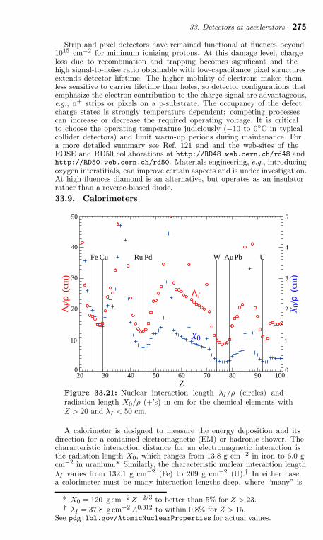
33. Detectors at accelerators 275
Strip and pixel detectors have remained functional at fluences beyond1015 cm−2 for minimum ionizing protons. At this damage level, chargeloss due to recombination and trapping becomes significant and thehigh signal-to-noise ratio obtainable with low-capacitance pixel structuresextends detector lifetime. The higher mobility of electrons makes themless sensitive to carrier lifetime than holes, so detector configurations thatemphasize the electron contribution to the charge signal are advantageous,e.g., n+ strips or pixels on a p-substrate. The occupancy of the defectcharge states is strongly temperature dependent; competing processescan increase or decrease the required operating voltage. It is criticalto choose the operating temperature judiciously (−10 to 0C in typicalcollider detectors) and limit warm-up periods during maintenance. Fora more detailed summary see Ref. 121 and and the web-sites of theROSE and RD50 collaborations at http://RD48.web.cern.ch/rd48 andhttp://RD50.web.cern.ch/rd50. Materials engineering, e.g., introducingoxygen interstitials, can improve certain aspects and is under investigation.At high fluences diamond is an alternative, but operates as an insulatorrather than a reverse-biased diode.
33.9. Calorimeters
20 30 50 70 9040 60 80 100Z
10
0
20
30
40
50
1
0
2
3
4
5
ΛI/
ρ (
cm)
ΛIX
0/ρ
(cm
)
X0
CuFe Ru Pd W Au Pb U
Figure 33.21: Nuclear interaction length λI/ρ (circles) andradiation length X0/ρ (+’s) in cm for the chemical elements withZ > 20 and λI < 50 cm.
A calorimeter is designed to measure the energy deposition and itsdirection for a contained electromagnetic (EM) or hadronic shower. Thecharacteristic interaction distance for an electromagnetic interaction isthe radiation length X0, which ranges from 13.8 g cm−2 in iron to 6.0 gcm−2 in uranium.* Similarly, the characteristic nuclear interaction lengthλI varies from 132.1 g cm−2 (Fe) to 209 g cm−2 (U).† In either case,a calorimeter must be many interaction lengths deep, where “many” is
* X0 = 120 g cm−2 Z−2/3 to better than 5% for Z > 23.† λI = 37.8 g cm−2 A0.312 to within 0.8% for Z > 15.
See pdg.lbl.gov/AtomicNuclearProperties for actual values.
276 33. Detectors at accelerators
determined by physical size, cost, and other factors. EM calorimeters tendto be 15–30 X0 deep, while hadronic calorimeters are usually compromisedat 5–8 λI . In real experiments there is likely to be an EM calorimeterin front of the hadronic section, which in turn has less sampling densityin the back, so the hadronic cascade occurs in a succession of differentstructures.
In all cases there is a premium on small λI/ρ and X0/ρ (both withunits of length). These quantities are shown for Z > 20 for the chemicalelements in Fig. 33.21.
These considerations are for sampling calorimeters consisting of metallicabsorber sandwiched or (threaded) with an active material which generatessignal. The active medium may be a scintillator, an ionizing noble liquid,a gas chamber, a semiconductor, or a Cherenkov radiator.
There are also homogeneous calorimeters, in which the entire volumeis sensitive, i.e., contributes signal. Homogeneous calorimeters (so farusually electromagnetic) may be built with inorganic heavy (high density,high 〈Z〉) scintillating crystals, or non-scintillating Cherenkov radiatorssuch as lead glass and lead fluoride. Scintillation light and/or ionizationin noble liquids can be detected. Nuclear interaction lengths in inorganiccrystals range from 17.8 cm (LuAlO3) to 42.2 cm (NaI).
33.9.1. Electromagnetic calorimeters :Revised October 2009 by R.-Y. Zhu (California Inst. of Technology).
The development of electromagnetic showers is discussed in the sectionon “Passage of Particles Through Matter” (Sec. 32 of this Review).
The energy resolution σE/E of a calorimeter can be parametrized as
a/√
E ⊕ b ⊕ c/E, where ⊕ represents addition in quadrature and E is inGeV. The stochastic term a represents statistics-related fluctuations suchas intrinsic shower fluctuations, photoelectron statistics, dead material atthe front of the calorimeter, and sampling fluctuations. For a fixed numberof radiation lengths, the stochastic term a for a sampling calorimeter isexpected to be proportional to
√
t/f , where t is plate thickness and fis sampling fraction [127,128]. While a is at a few percent level for ahomogeneous calorimeter, it is typically 10% for sampling calorimeters.The main contributions to the systematic, or constant, term b aredetector non-uniformity and calibration uncertainty. In the case of thehadronic cascades discussed below, non-compensation also contributes tothe constant term. One additional contribution to the constant term forcalorimeters built for modern high-energy physics experiments, operatedin a high-beam intensity environment, is radiation damage of the activemedium. This can be minimized by developing radiation-hard activemedia [48] and by frequent in situ calibration and monitoring [47,128].
33.9.2. Hadronic calorimeters : [1–5,133]Revised September 2013 by D. E. Groom (LBNL).
Most large hadron calorimeters are parts of large 4π detectors atcolliding beam facilities. At present these are sampling calorimeters:plates of absorber (Fe, Pb, Cu, or occasionally U or W) alternating withplastic scintillators (plates, tiles, bars), liquid argon (LAr), or gaseousdetectors. The ionization is measured directly, as in LAr calorimeters, orvia scintillation light observed by photodetectors (usually PMT’s or siliconphotodiodes). Wavelength-shifting fibers are often used to solve difficultproblems of geometry and light collection uniformity. Silicon sensors arebeing studied for ILC detectors; in this case e-h pairs are collected.
In an inelastic hadronic collision a significant fraction fem of theenergy is removed from further hadronic interaction by the production
33. Detectors at accelerators 277
of secondary π0’s and η’s, whose decay photons generate high-energyelectromagnetic (EM) cascades. Charged secondaries (π±, p, . . . ) depositenergy via ionization and excitation, but also interact with nuclei,producing spallation protons and neutrons, evaporation neutrons, andrecoiling nuclei in highly excited states. The charged collision productsproduce detectable ionization, as do the showering γ-rays from the promptde-excitation of highly excited nuclei. The recoiling nuclei generate littleor no detectable signal. The neutrons lose kinetic energy in elasticcollisions over hundreds of ns, gradually thermalize and are captured,with the production of more γ-rays—usually outside the acceptance gateof the electronics. Between endothermic spallation losses, nuclear recoils,and late neutron capture, a significant fraction of the hadronic energy(20%–40%, depending on the absorber and energy of the incident particle)is invisible.
For 〈h/e〉 6= 1 (noncompensation), where h and e are the hadronicand electromagnetic calorimeter responses, respectively, fluctuations infem significantly contribute to or even dominate the resolution. Sincethe fem distribution has a high-energy tail, the calorimeter response isnon-Gaussian with a high-energy tail if 〈h/e〉 < 1. Noncompensation thusseriously degrades resolution and produces a nonlinear response.
It is clearly desirable to compensate the response, i.e., to design thecalorimeter such that 〈h/e〉 = 1. This is possible only with a samplingcalorimeter, where several variables can be chosen or tuned:1. Decrease the EM sensitivity. EM cross sections increase with Z,
and most of the energy in an EM shower is deposited by low-energy electrons. A disproportionate fraction of the EM energy isthus deposited in the higher-Z absorber. The degree of EM signalsuppression can be somewhat controlled by tuning the sensor/absorberthickness ratio.
2. Increase the hadronic sensitivity. The abundant neutrons have alarge n-p scattering cross section, with the production of low-energyscattered protons in hydrogenous sampling materials such as butane-filled proportional counters or plastic scintillator. (When scattering offa nucleus with mass number A, a neutron can at most lose 4A/(1+A)2
of its kinetic energy.)3. Fabjan and Willis proposed that the additional signal generated in the
aftermath of fission in 238U absorber plates should compensate nuclearfluctuations [146].Motivated very much by the work of Brau, Gabriel, Bruckmann, and
Wigmans [148], several groups built calorimeters which were very nearlycompensating. The degree of compensation was sensitive to the acceptancegate width, and so could be somewhat tuned.
After the first interaction of the incident hadron, the averagelongitudinal distribution rises to a smooth peak. The peak positionincreases slowly with energy. The distribution becomes reasonablyexponential after several interaction lengths. A gamma distribution fairlywell describes the longitudinal development of an EM shower, as discussedin Sec. 32.5.
The transverse energy deposit is characterized by a central coredominated by EM cascades, together with a wide “skirt” produced bywide-angle hadronic interactions [154].
Further discussion and all references may be found in the full Reviewof Particle Physics.The numbering of references and equations used herecorresponds to that version.
278 34. Detectors for non-accelerator physics
34. PARTICLE DETECTORS FOR
NON-ACCELERATOR PHYSICS
Revised 2013 (see the various sections for authors).
34.1. Introduction
Non-accelerator experiments have become increasingly important inparticle physics. These include classical cosmic ray experiments, neutrinooscillation measurements, and searches for double-beta decay, darkmatter candidates, and magnetic monopoles. The experimental methodsare sometimes those familiar at accelerators (plastic scintillators, driftchambers, TRD’s, etc.) but there is also instrumentation either notfound at accelerators or applied in a radically different way. Examplesare atmospheric scintillation detectors (Fly’s Eye), massive Cherenkovdetectors (Super-Kamiokande, IceCube), ultracold solid state detectors(CDMS). And, except for the cosmic ray detectors, there is a demand forradiologically ultra-pure materials.
In this section, some more important detectors special to terrestrialnon-accelerator experiments are discussed. Techniques used in bothaccelerator and non-accelerator experiments are described in Sec. 33,Particle Detectors at Accelerators, some of which have been modified toaccommodate the non-accelerator nuances. Space-based detectors also usesome unique methods, but these are beyond the present scope of RPP.
34.2. High-energy cosmic-ray hadron and gamma-ray
detectors34.2.1. Atmospheric fluorescence detectors :
Revised August 2013 by L.R. Wiencke (Colorado School of Mines).
Cosmic-ray fluorescence detectors (FD) use the atmosphere as agiant calorimeter to measure isotropic scintillation light that traces thedevelopment profiles of extensive air showers (EAS). The EASs observedare produced by the interactions of high-energy (E > 1017eV) subatomicparticles in the stratosphere and upper troposphere. The amount ofscintillation light generated is proportional to energy deposited in theatmosphere and nearly independent of the primary species.
The scintillation light is emitted between 290 and 430 nm, whenrelativistic charged particles, primarily electrons and positrons, excitenitrogen molecules in air, resulting in transitions of the 1P and 2P systems.
An FD element (telescope) consists of a non-tracking spherical mirror(3.5–13 m2 and less than astronomical quality), a close-packed “camera”of PMTs near the focal plane, and flash ADC readout system with a pulseand track-finding trigger scheme [10]. Simple reflector optics (12 × 16
degree field of view (FOV) on 256 PMTs) and Schmidt optics (30 × 30
on 440 PMTs), including a correcting element, have been used.
The EAS generates a track consistent with a light source moving atv = c across the FOV. The number of photons (Nγ) as a function ofatmospheric depth (X) can be expressed as [8]
dNγ
dX=
dEtotdep
dX
∫
Y (λ, P, T, u) · τatm(λ, X) · εFD(λ)dλ , (34.1)
where τatm(λ, X) is atmospheric transmission, including wavelength (λ)dependence, and εFD(λ) is FD efficiency. εFD(λ) includes geometric factors
34. Detectors for non-accelerator physics 279
and collection efficiency of the optics, quantum efficiency of the PMTs, andother throughput factors. The typical systematic uncertainties, Y (10%),τatm (10%) and εFD (photometric calibration 10%), currently dominatethe total reconstructed EAS energy uncertainty. ∆E/E of 20–25% ispossible, provided the geometric fit of the EAS axis is constrained bymulti-eye stereo projection, or by timing from a colocated sparse array ofsurface detectors.
34.2.2. Atmospheric Cherenkov telescopes for high-energy γ-
ray astronomy :
Updated August 2013 by J. Holder (Dept. of Phys. and Astronomy &Bartol Research Inst., Univ. of Delaware).
Atmospheric Cherenkov detectors achieve effective collection areas of∼ 105 m2 by employing the Earth’s atmosphere as an intrinsic part of thedetection technique. A hadronic cosmic ray or high energy γ-ray incidenton the Earth’s atmosphere triggers a particle cascade, or air shower.Relativistic charged particles in the cascade produce Cherenkov radiation,which is emitted along the shower direction, resulting in a light pool onthe ground with a radius of ∼ 130 m. Maximum emission occurs whenthe number of particles in the cascade is largest. The Cherenkov light atground level peaks at a wavelength, λ ≈ 300–350 nm. The photon densityis typically ∼ 100 photons/m2 at 1 TeV, arriving in a brief flash of a fewnanoseconds duration.
Modern atmospheric Cherenkov telescopes consist of large (> 100m2)segmented mirrors on steerable altitude-azimuth mounts. A camera, madefrom an array of up to 1000 photomultiplier tubes (PMTs) covering afield-of-view of up to 5.0 in diameter, is placed at the mirror focus andused to record a Cherenkov image of each air shower. Images are recordedat a rate of a few hundred Hz, the vast majority of which are due toshowers with hadronic cosmic-ray primaries. The shape and orientation ofthe Cherenkov images are used to discriminate γ-ray photon events fromthis cosmic-ray background, and to reconstruct the photon energy andarrival direction.
The total Cherenkov yield from the air shower is proportional to theenergy of the primary particle. The energy resolution of this technique,also energy-dependent, is typically 15–20% at energies above a few hundredGeV. Energy spectra of γ-ray sources can be measured over a wide range;potentially from ∼ 50 GeV to ∼ 100 TeV, depending upon the instrumentcharacteristics, source strength, and exposure time.
34.3. Large neutrino detectors
34.3.1. Deep liquid detectors for rare processes :
Revised September 2013 by K. Scholberg & C.W. Walter (DukeUniversity).
Deep, large detectors for rare processes tend to be multi-purposewith physics reach that includes not only solar, reactor, supernova andatmospheric neutrinos, but also searches for baryon number violation,searches for exotic particles such as magnetic monopoles, and neutrinoand cosmic ray astrophysics in different energy regimes. The detectorsmay also serve as targets for long-baseline neutrino beams for neutrinooscillation physics studies. In general, detector design considerations canbe divided into high-and low-energy regimes, for which background and
280 34. Detectors for non-accelerator physics
event reconstruction issues differ. The high-energy regime, from about100 MeV to a few hundred GeV, is relevant for proton decay searches,atmospheric neutrinos and high-energy astrophysical neutrinos. Thelow-energy regime (a few tens of MeV or less) is relevant for supernova,solar, reactor and geological neutrinos.
Large water Cherenkov and scintillator detectors (see Table 34.1)usually consist of a volume of transparent liquid viewed by photomultipliertubes (PMTs). Because photosensors lining an inner surface represent adriving cost that scales as surface area, very large volumes can be usedfor comparatively reasonable cost. A common configuration is to have atleast one concentric outer layer of liquid material separated from the innerpart of the detector to serve as shielding against ambient background. Ifoptically separated and instrumented with PMTs, an outer layer may alsoserve as an active veto against entering cosmic rays and other background
Because in most cases one is searching for rare events, large detectorsare usually sited underground to reduce cosmic-ray related background(see Chapter 28). The minimum depth required varies according to thephysics goals [27].
34.3.1.1. Liquid scintillator detectors:
Past and current large underground detectors based on hydrocarbonscintillators include LVD, MACRO, Baksan, Borexino, KamLAND andSNO+. Experiments at nuclear reactors include Chooz, Double Chooz,Daya Bay, and RENO. Organic liquid scintillators for large detectorsare chosen for high light yield and attenuation length, good stability,compatibility with other detector materials, high flash point, low toxicity,appropriate density for mechanical stability, and low cost.
Scintillation detectors have an advantage over water Cherenkovdetectors in the lack of Cherenkov threshold and the high light yield.However, scintillation light emission is nearly isotropic, and thereforedirectional capabilities are relatively weak.
34.3.1.2. Water Cherenkov detectors:
Very large-imaging water detectors reconstruct ten-meter-scaleCherenkov rings produced by charged particles (see Sec. 33.5.0).The first such large detectors were IMB and Kamiokande. The onlycurrently existing instance of this class is Super-Kamiokande (Super-K).
Cherenkov detectors are excellent electromagnetic calorimeters, and thenumber of Cherenkov photons produced by an e/γ is nearly proportionalto its kinetic energy. The number of collected photoelectrons dependson the scattering and attenuation in the water along with the photo-cathode coverage, quantum efficiency and the optical parameters of anyexternal light collection systems or protective material surrounding them.Event-by-event corrections are made for geometry and attenuation.
High-energy (∼100 MeV or more) neutrinos from the atmosphere orbeams interact with nucleons; for the nucleons bound inside the 16Onucleus, the nuclear effects both at the interaction, and as the particlesleave the nucleus must be considered when reconstructing the interaction.Various event topologies can be distinguished by their timing and fitpatterns, and by presence or absence of light in a veto.
Low-energy neutrino interactions of solar neutrinos in water arepredominantly elastic scattering off atomic electrons; single electron eventsare then reconstructed. At solar neutrino energies, the visible energy
34. Detectors for non-accelerator physics 281
resolution (∼ 30%/√
ξ Evis(MeV)) is about 20% worse than photoelectroncounting statistics would imply. At these energies, radioactive backgroundsbecome a dominant issue.
The Sudbury Neutrino Observatory (SNO) detector [32] is the onlyinstance of a large heavy water detector and deserves mention here. Inaddition to an outer 1.7 kton of light water, SNO contained 1 kton of D2O,giving it unique sensitivity to neutrino neutral current (νx+d → νx+p+n),and charged current (νe + d → p + p + e−) deuteron breakup reactions.
34.3.3. Coherent radio Cherenkov radiation detectors :
Revised February 2013 by S.R. Klein (LBNL/UC Berkeley).
Radio detectors sensitive to coherent Cherenkov radiation provide anattractive way to search for ultra-high energy cosmic neutrinos, the onlylong-range probe of the ultra-high energy cosmos.
Electromagnetic and hadronic showers produce radio pulses via theAskaryan effect [30], as discussed in Sec. 30. The shower contains moreelectrons than positrons, leading to coherent emission. The electric fieldstrength is proportional to the neutrino energy; the radiated power goesas its square. Detectors with antennas placed in the active volume havethresholds around 1017 eV. The electric field strength increases linearlywith frequency, up to a cut-off wavelength set by the transverse size ofthe shower. The cut-off is about 1 GHz in ice, and 2.5 GHz in rock/lunarregolith. The signal is linearly polarized pointing toward the shower axis.This polarization is a key diagnostic for radiodetection, and can be usedto help determine the neutrino direction.
34.3.3.1. The Moon as a target:
Because of it’s large size and non-conducting regolith, and theavailability of large radio-telescopes, the moon is an attractive target[45]; Conventional radio-telescopes are reasonably well matched to lunarneutrino searches, with natural beam widths not too dissimilar from thesize of the Moon. The big limitation of lunar experiments is that the240,000 km target-antenna separation leads to neutrino energy thresholdsfar above 1020 eV.
Experiments so far include Parkes, Glue, NuMoon, Lunaska, and Resun.No signals have been detected. These efforts have considerable scope forexpansion. In the near future, several large radio detector arrays shouldreach significantly lower limits. The LOFAR array is beginning to takedata with 36 detector clusters spread over Northwest Europe [46]. In thelonger term, the Square Kilometer Array (SKA) with 1 km2 effective areawill push thresholds down to near 1020 eV.
34.3.3.2. The ANITA balloon experiment:
The ANITA balloon experiment made two flights around Antarctica,floating at an altitude around 35 km [47]. Its 40 (32 in the first flight)dual-polarization horn antennas scanned the surrounding ice, out to thehorizon (650 km away). Because of the small angle of incidence, ANITAwas able to make use of polarization information; ν signals should bevertically polarized, while most background from cosmic-ray air showersis expected to be horizontally polarized. By using the several-meterseparation between antennas, ANITA achieved a pointing accuracy of0.2–0.40 in elevation, and 0.5–1.10 in azimuth.
The attenuation length of radio waves depends on the frequencyand ice temperature, with attenuation higher in warmer ice. A recent
282 34. Detectors for non-accelerator physics
measurement, by the ARA collaboration at the South Pole found anaverage attenuation length of 670+180
−66 m [48]. On the Ross Ice Shelf,ARIANNA finds attenuation lengths of 300–500 m, depending onfrequency [49].
ANITA verified the accuracy of their calibrations by observing radiosources that they buried in the ice. ANITA has also recently observedradio waves from cosmic-ray air showers; these showers are differentiatedfrom neutrino showers on the basis of the radio polarization and zenithangle distribution [50].
34.3.3.3. Active Volume Detectors:
The use of radio antennas located in the active volume was pioneeredby the RICE experiment, which buried radio antennas in holes drilled forAMANDA [51] at the South Pole. RICE was comprised of 18 half-wavedipole antennas, sensitive from 200 MHz to 1 GHz, buried between 100and 300 m deep. The array triggered when four or more stations fireddiscriminators within 1.2 µs, giving it a threshold of about 1017 eV.
Two groups are prototyping detectors, with the goal of a detector withan active volume in the 100 km3 range. Both techniques are modular, sothe detector volume scales roughly linearly with the available funding.The Askaryan Radio Array (ARA) is located at the South Pole, while theAntarctic Ross Iceshelf ANtenna Neutrino Array (ARIANNA) is on theRoss Ice Shelf. Both experiments use local triggers based on a coincidencebetween multiple antennas in a single station/cluster.
ARIANNA will be located in Moore’s Bay, on the Ross Ice Shelf, where≈ 575m of ice sits atop the Ross Sea [49]. The site was chosen because theice-seawater interface is smooth there, so the interface acts as a mirror forradio waves. The major advantage of this approach is that ARIANNA issensitive to downward going neutrinos, and should be able to see more ofthe Cherenkov cone for horizontal neutrinos. One disadvantage of the siteis that the ice is warmer, so the radio attenuation length will be shorter.
34.4. Large time-projection chambers for rare event
detection
Written August 2009 by M. Heffner (LLNL).
TPCs in non-accelerator particle physics experiments are principallyfocused on rare event detection (e.g., neutrino and dark matterexperiments) and the physics of these experiments can place dramaticallydifferent constraints on the TPC design (only extensions of the traditionalTPCs are discussed here). The drift gas or liquid is usually the target ormatter under observation and due to very low signal rates a TPC withthe largest possible active mass is desired. The large mass complicatesparticle tracking of short and sometimes very low-energy particles. Otherspecial design issues include efficient light collection, background rejection,internal triggering, and optimal energy resolution.
The liquid-phase TPC can have a high density at low pressure thatresults in very good self-shielding and compact installation with lightweightcontainment. The down sides are the need for cryogenics, slower chargedrift, tracks shorter than typical electron diffusion distances, lower-energyresolution (e.g., xenon) and limited charge readout options. Slower chargedrift requires long electron lifetimes, placing strict limits on the oxygenand other impurities with high electron affinity.
34. Detectors for non-accelerator physics 283
A high-pressure gas phase TPC has no cryogenics and density is easilyoptimized for the signal, but a large heavy-pressure vessel is required.Although self shielding is reduced, it can in some cases approach that ofthe liquid phase; in xenon at 50 atm the density is about half that of wateror about 1/6 of liquid xenon. A significant feature of high pressure xenongas is the energy resolution.
Rare-event TPCs can be designed to detect scintillation light as well ascharge to exploit the anti-correlation to improve energy resolution and/orsignal to noise [41]. Electroluminescence can be used to proportionallyamplify the drifted ionization, and it does not suffer the fluctuations ofan avalanche or the small signals of direct collection. It works by settingup at the positive end of the drift volume parallel meshes or wire arrayswith an electric field larger than the drift field, but less than the fieldneeded for avalanche. In xenon, this is 3–6 kV cm−1 bar−1 for good energyresolution.
Differentiation of nuclear and electron recoils at low-energy deposition isimportant as a means of background rejection. The nuclear recoil depositsa higher density of ionization than an electron recoil and this results ina higher geminate recombination resulting in a higher output of primaryscintillation and lower charge. The ratio of scintillation to charge can beused to distinguish the two. In the case of an electroluminescence readout,this is done simply with the ratio of primary light to secondary light.
34.5. Sub-Kelvin detectorsWritten September 2009 by S. Golwala (Caltech).
Detectors operating below 1 K, also known as “low-temperature”or “cryogenic” detectors, use <∼meV quanta (phonons, superconductingquasiparticles) to provide better energy resolution than is typicallyavailable from conventional technologies. Such resolution can provideunique advantages to applications reliant on energy resolution, suchas beta-decay experiments seeking to measure the νe mass or searchesfor neutrinoless double-beta decay. In addition, the sub-Kelvin modeis combined with conventional (eV quanta) ionization or scintillationmeasurements to provide discrimination of nuclear recoils from electronrecoils, critical for searches for WIMP dark matter and for coherentneutrino-nucleus scattering.34.5.1. Thermal Phonons :
The most basic kind of low-temperature detector employs a dielectricabsorber coupled to a thermal bath via a weak link. A thermistor monitorsthe temperature of the absorber. The energy E deposited by a particleinteraction causes a calorimetric temperature change by increasing thepopulation of thermal phonons. The fundamental sensitivity is
σ2E = ξ2kT [T C(T ) + βE] , (34.5)
where C is the heat capacity of the detector, T is the temperature ofoperation, k is Boltzmann’s constant, and ξ is a dimensionless factor oforder unity that is precisely calculable from the nature of the thermal linkand the non-thermodynamic noises (e.g., Johnson and/or readout noise).The energy resolution typically acquires an additional energy dependencedue to deviations from an ideal calorimetric model that cause positionand/or energy dependence in the signal shape. The rise time of responseis limited by the internal thermal conductivity of the absorber.
284 34. Detectors for non-accelerator physics
34.5.2. Athermal Phonons and Superconducting Quasiparticles :
The advantage of thermal phonons is also a disadvantage: energyresolution degrades as
√M where M is the detector mass. This motivates
the use of athermal phonons. There are three steps in the development ofthe phonon signal. The recoiling particle deposits energy along its track,with the majority going directly into phonons. The recoil and bandgapenergy scales (keV and higher, and eV, respectively) are much largerthan phonon energies (meV), so the full energy spectrum of phonons ispopulated, with phase space favoring the most energetic phonons.
Another mode is detection of superconducting quasiparticles insuperconducting crystals. Energy absorption breaks superconductingCooper pairs and yields quasiparticles, electron-like excitations that candiffuse through the material and that recombine after the quasiparticlelifetime.
34.5.3. Ionization and Scintillation :
While ionization and scintillation detectors usually operate at muchhigher temperatures, ionization and scintillation can be measured atlow temperature and can be combined with a “sub-Kelvin” techniqueto discriminate nuclear recoils from background interactions producingelectron recoils, which is critical for WIMP searches and coherentneutrino-nucleus scattering. With ionization, such techniques are based onLindhard theory [50], which predicts substantially reduced ionization yieldfor nuclear recoils relative to electron recoils. For scintillation, applicationof Birks’ law Sec. 28.3.0) yields a similar prediction.
34.6. Low-radioactivity background techniques
Revised July 2013 by A. Piepke (University of Alabama).
The physics reach of low-energy rare event searches e.g. for dark matter,neutrino oscillations, or double beta decay is often limited by backgroundcaused by radioactivity. Depending on the chosen detector design, theseparation of the physics signal from this unwanted interference can beachieved on an event-by-event basis by active event tagging, utilizingsome unique event feature, or by reducing the radiation backgroundby appropriate shielding and material selection. In both cases, thebackground rate is proportional to the flux of background-creatingradiation. Its reduction is thus essential for realizing the full physicspotential of the experiment. In this context, “low energy” may be definedas the regime of natural, anthropogenic, or cosmogenic radioactivity, all atenergies up to about 10 MeV. Following the classification of [64], sourcesof background may be categorized into the following classes:
1. environmental radioactivity,
2. radioimpurities in detector or shielding components,
3. radon and its progeny,
4. cosmic rays,
5. neutrons from natural fission, (α, n) reactions and from cosmic-raymuon spallation and capture.
Further discussion and all references may be found in the full Review
of Particle Physics.The numbering of references and equations used herecorresponds to that version.
35. Radioactivity and radiation protection 285
35. RADIOACTIVITY AND RADIATION PROTECTION
Revised August 2013 by S. Roesler and M. Silari (CERN).
35.1. Definitions
The International Commission on Radiation Units and Measurements(ICRU) recommends the use of SI units. Therefore we list SI units first,followed by cgs (or other common) units in parentheses, where they differ.
• Activity (unit: Becquerel):
1 Bq = 1 disintegration per second (= 27 pCi).
• Absorbed dose (unit: gray): The absorbed dose is the energyimparted by ionizing radiation in a volume element of a specified materialdivided by the mass of this volume element.
1 Gy = 1 J/kg (= 104 erg/g = 100 rad)
= 6.24 × 10¹² MeV/kg deposited energy.
• Kerma (unit: gray): Kerma is the sum of the initial kinetic energies ofall charged particles liberated by indirectly ionizing particles in a volumeelement of the specified material divided by the mass of this volumeelement.
• Exposure (unit: C/kg of air [= 3880 Roentgen†]): The exposure isa measure of photon fluence at a certain point in space integrated overtime, in terms of ion charge of either sign produced by secondary electronsin a small volume of air about the point. Implicit in the definition isthe assumption that the small test volume is embedded in a sufficientlylarge uniformly irradiated volume that the number of secondary electronsentering the volume equals the number leaving (so-called charged particleequilibrium).
Table 35.1: Radiation weighting factors, wR.
Radiation type wR
Photons 1Electrons and muons 1Neutrons, En < 1 MeV 2.5 + 18.2 × exp[−(lnEn)2/6]
1 MeV ≤ En ≤ 50 MeV 5.0 + 17.0 × exp[−(ln(2En))2/6]En > 50 MeV 2.5 + 3.25 × exp[−(ln(0.04En))2/6]
Protons and charged pions 2Alpha particles, fissionfragments, heavy ions 20
• Equivalent dose (unit: Sievert [= 100 rem (roentgen equivalent inman)]): The equivalent dose HT in an organ or tissue T is equal to thesum of the absorbed doses DT,R in the organ or tissue caused by differentradiation types R weighted with so-called radiation weighting factors wR:
HT =∑
R
wR × DT,R . (35.1)
† This unit is somewhat historical, but appears on some measuring in-struments. One R is the amount of radiation required to liberate positiveand negative charges of one electrostatic unit of charge in 1 cm3 of air atstandard temperature and pressure (STP)
286 35. Radioactivity and radiation protection
It expresses long-term risks (primarily cancer and leukemia) from low-levelchronic exposure. The values for wR recommended recently by ICRP [2]are given in Table 35.1.
• Effective dose (unit: Sievert): The sum of the equivalent doses,weighted by the tissue weighting factors wT (
∑T wT = 1) of several organs
and tissues T of the body that are considered to be most sensitive [2], iscalled “effective dose” E:
E =∑
T
wT × HT . (35.2)
35.2. Radiation levels [4]
• Natural annual background, all sources: Most world areas, whole-body equivalent dose rate ≈ (1.0–13) mSv (0.1–1.3 rem). Can range upto 50 mSv (5 rem) in certain areas. U.S. average ≈ 3.6 mSv, including≈ 2 mSv (≈ 200 mrem) from inhaled natural radioactivity, mostly radonand radon daughters. (Average is for a typical house and varies by morethan an order of magnitude. It can be more than two orders of magnitudehigher in poorly ventilated mines. 0.1–0.2 mSv in open areas.)
• Cosmic ray background (sea level, mostly muons):∼ 1 min−1 cm−2 sr−1. For more accurate estimates and details, see theCosmic Rays section (Sec. 28 of this Review).
• Fluence (per cm2) to deposit one Gy, assuming uniform irradiation:
≈ (charged particles) 6.24×10⁹/(dE/dx), where dE/dx (MeVg−1 cm2), the energy loss per unit length, may be obtained from Figs.32.2 and 32.4 in Sec. 32 of the Review, and pdg.lbl.gov/AtomicNuclear
Properties.
≈ 3.5 × 109 cm−2 minimum-ionizing singly-charged particles in carbon.
≈ (photons) 6.24×10⁹/[Ef/ℓ], for photons of energy E (MeV),attenuation length ℓ (g cm−2), and fraction f . 1 expressing the fractionof the photon’s energy deposited in a small volume of thickness ≪ ℓ butlarge enough to contain the secondary electrons.
≈ 2 × 10¹¹ photons cm−2 for 1 MeV photons on carbon (f ≈ 1/2).
35.3. Health effects of ionizing radiation
• Recommended limits of effective dose to radiation workers(whole-body dose):∗
EU/Switzerland: 20 mSv yr−1
U.S.: 50 mSv yr−1 (5 rem yr−1)†
• Lethal dose: The whole-body dose from penetrating ionizing radiationresulting in 50% mortality in 30 days (assuming no medical treatment)is 2.5–4.5 Gy (250–450 rad), as measured internally on body longitudinalcenter line. Surface dose varies due to variable body attenuation and maybe a strong function of energy.
• Cancer induction by low LET radiation: The cancer inductionprobability is about 5% per Sv on average for the entire population [2].
Footnotes:
∗ The ICRP recommendation [2] is 20 mSv yr−1 averaged over 5 years,with the dose in any one year ≤ 50 mSv.
† Many laboratories in the U.S. and elsewhere set lower limits.
See full Review for references and further details.
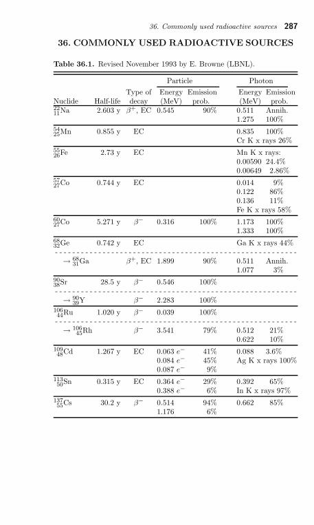
36. Commonly used radioactive sources 287
36. COMMONLY USED RADIOACTIVE SOURCES
Table 36.1. Revised November 1993 by E. Browne (LBNL).
Particle Photon
Type of Energy Emission Energy EmissionNuclide Half-life decay (MeV) prob. (MeV) prob.2211
Na 2.603 y β+, EC 0.545 90% 0.511 Annih.1.275 100%
5425Mn 0.855 y EC 0.835 100%
Cr K x rays 26%5526
Fe 2.73 y EC Mn K x rays:0.00590 24.4%0.00649 2.86%
5727
Co 0.744 y EC 0.014 9%0.122 86%0.136 11%Fe K x rays 58%
6027
Co 5.271 y β− 0.316 100% 1.173 100%1.333 100%
6832
Ge 0.742 y EC Ga K x rays 44%- - - - - - - - - - - - - - - - - - - - - - - - - - - - - - - - - - - - - - - - - - - - - - - - - - - - - - - -
→ 6831
Ga β+, EC 1.899 90% 0.511 Annih.1.077 3%
9038
Sr 28.5 y β− 0.546 100%- - - - - - - - - - - - - - - - - - - - - - - - - - - - - - - - - - - - - - - - - - - - - - - - - - - - - - - -
→ 9039
Y β− 2.283 100%
10644
Ru 1.020 y β− 0.039 100%- - - - - - - - - - - - - - - - - - - - - - - - - - - - - - - - - - - - - - - - - - - - - - - - - - - - - - - -
→ 10645
Rh β− 3.541 79% 0.512 21%0.622 10%
10948
Cd 1.267 y EC 0.063 e− 41% 0.088 3.6%0.084 e− 45% Ag K x rays 100%0.087 e− 9%
11350
Sn 0.315 y EC 0.364 e− 29% 0.392 65%0.388 e− 6% In K x rays 97%
13755
Cs 30.2 y β− 0.514 94% 0.662 85%1.176 6%
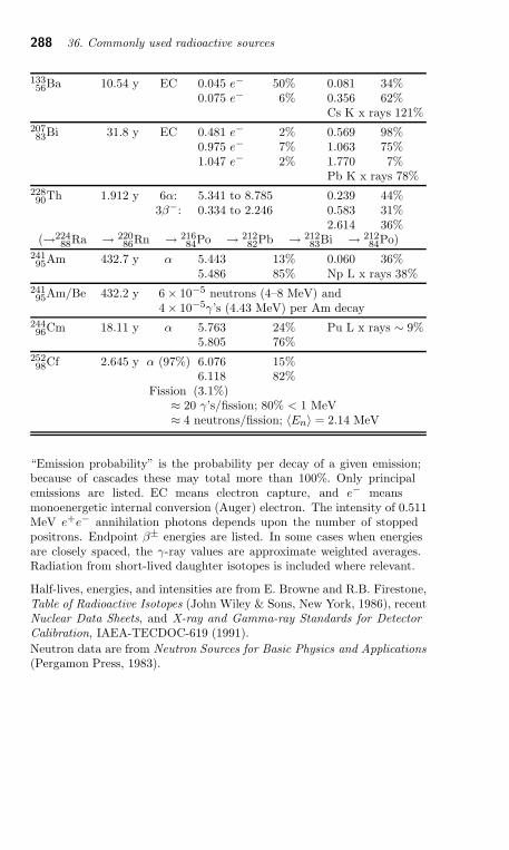
288 36. Commonly used radioactive sources
13356
Ba 10.54 y EC 0.045 e− 50% 0.081 34%0.075 e− 6% 0.356 62%
Cs K x rays 121%20783
Bi 31.8 y EC 0.481 e− 2% 0.569 98%0.975 e− 7% 1.063 75%1.047 e− 2% 1.770 7%
Pb K x rays 78%22890
Th 1.912 y 6α: 5.341 to 8.785 0.239 44%3β−: 0.334 to 2.246 0.583 31%
2.614 36%(→224
88Ra → 220
86Rn → 216
84Po → 212
82Pb → 212
83Bi → 212
84Po)
24195
Am 432.7 y α 5.443 13% 0.060 36%5.486 85% Np L x rays 38%
24195
Am/Be 432.2 y 6 × 10⁻⁵ neutrons (4–8 MeV) and4 × 10−5γ’s (4.43 MeV) per Am decay
24496
Cm 18.11 y α 5.763 24% Pu L x rays ∼ 9%5.805 76%
25298
Cf 2.645 y α (97%) 6.076 15%6.118 82%
Fission (3.1%)≈ 20 γ’s/fission; 80% < 1 MeV≈ 4 neutrons/fission; 〈En〉 = 2.14 MeV
“Emission probability” is the probability per decay of a given emission;because of cascades these may total more than 100%. Only principalemissions are listed. EC means electron capture, and e− meansmonoenergetic internal conversion (Auger) electron. The intensity of 0.511MeV e+e− annihilation photons depends upon the number of stoppedpositrons. Endpoint β± energies are listed. In some cases when energiesare closely spaced, the γ-ray values are approximate weighted averages.Radiation from short-lived daughter isotopes is included where relevant.
Half-lives, energies, and intensities are from E. Browne and R.B. Firestone,Table of Radioactive Isotopes (John Wiley & Sons, New York, 1986), recentNuclear Data Sheets, and X-ray and Gamma-ray Standards for Detector
Calibration, IAEA-TECDOC-619 (1991).
Neutron data are from Neutron Sources for Basic Physics and Applications
(Pergamon Press, 1983).
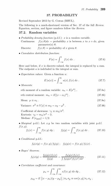
37. Probability 289
37. PROBABILITY
Revised September 2013 by G. Cowan (RHUL).
The following is a much-shortened version of Sec. 37 of the full Review.Equation, section, and figure numbers follow the Review.
37.2. Random variables
• Probability density function (p.d.f.): x is a random variable.
Continuous: f(x; θ)dx = probability x is between x to x + dx, givenparameter(s) θ;
Discrete: f(x; θ) = probability of x given θ.
• Cumulative distribution function:
F (a) =
∫ a
−∞
f(x) dx . (37.6)
Here and below, if x is discrete-valued, the integral is replaced by a sum.The endpoint a is indcluded in the integral or sum.
• Expectation values: Given a function u:
E [u(x)] =
∫
∞
−∞
u(x) f(x) dx . (37.7)
• Moments:
nth moment of a random variable: αn = E[xn] , (37.8a)
nth central moment: mn = E[(x − α1)n] . (37.8b)
Mean: µ ≡ α1 . (37.9a)
Variance: σ2 ≡ V [x] ≡ m2 = α2 − µ2 . (37.9b)
Coefficient of skewness: γ1 ≡ m3/σ3.
Kurtosis: γ2 = m4/σ4 − 3 .
Median: F (xmed) = 1/2.
• Marginal p.d.f.: Let x,y be two random variables with joint p.d.f.f(x, y).
f1(x) =
∫
∞
−∞
f(x, y) dy ; f2(y) =
∫
∞
−∞
f(x, y) dx . (37.10)
• Conditional p.d.f.:
f4(x|y) = f(x, y)/f2(y) ; f3(y|x) = f(x, y)/f1(x) .
• Bayes’ theorem:
f4(x|y) =f3(y|x)f1(x)
f2(y)=
f3(y|x)f1(x)∫
f3(y|x′)f1(x′) dx′. (37.11)
• Correlation coefficient and covariance:
µx =
∫
∞
−∞
∫
∞
−∞
xf(x, y) dx dy , (37.12)
ρxy = E[
(x − µx)(y − µy)]
/σx σy ≡ cov[x, y]/σx σy ,
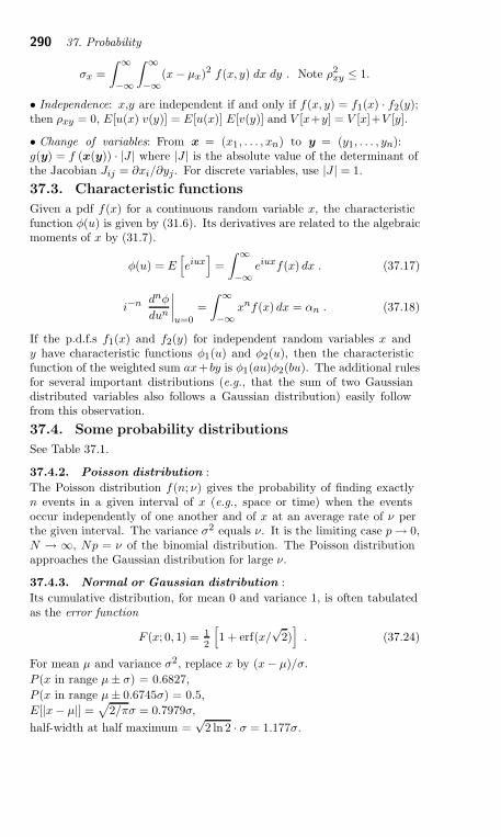
290 37. Probability
σx =
∫
∞
−∞
∫
∞
−∞
(x − µx)2 f(x, y) dx dy . Note ρ2xy ≤ 1.
• Independence: x,y are independent if and only if f(x, y) = f1(x) · f2(y);then ρxy = 0, E[u(x) v(y)] = E[u(x)] E[v(y)] and V [x+y] = V [x]+V [y].
• Change of variables: From x = (x1, . . . , xn) to y = (y1, . . . , yn):g(y) = f (x(y)) · |J | where |J | is the absolute value of the determinant ofthe Jacobian Jij = ∂xi/∂yj. For discrete variables, use |J | = 1.
37.3. Characteristic functions
Given a pdf f(x) for a continuous random variable x, the characteristicfunction φ(u) is given by (31.6). Its derivatives are related to the algebraicmoments of x by (31.7).
φ(u) = E[
eiux]
=
∫
∞
−∞
eiuxf(x) dx . (37.17)
i−n dnφ
dun
∣
∣
∣
∣
u=0=
∫
∞
−∞
xnf(x) dx = αn . (37.18)
If the p.d.f.s f1(x) and f2(y) for independent random variables x andy have characteristic functions φ1(u) and φ2(u), then the characteristicfunction of the weighted sum ax+ by is φ1(au)φ2(bu). The additional rulesfor several important distributions (e.g., that the sum of two Gaussiandistributed variables also follows a Gaussian distribution) easily followfrom this observation.
37.4. Some probability distributions
See Table 37.1.
37.4.2. Poisson distribution :
The Poisson distribution f(n; ν) gives the probability of finding exactlyn events in a given interval of x (e.g., space or time) when the eventsoccur independently of one another and of x at an average rate of ν perthe given interval. The variance σ2 equals ν. It is the limiting case p → 0,N → ∞, Np = ν of the binomial distribution. The Poisson distributionapproaches the Gaussian distribution for large ν.
37.4.3. Normal or Gaussian distribution :
Its cumulative distribution, for mean 0 and variance 1, is often tabulatedas the error function
F (x; 0, 1) = 12
[
1 + erf(x/√
2)]
. (37.24)
For mean µ and variance σ2, replace x by (x − µ)/σ.
P (x in range µ ± σ) = 0.6827,
P (x in range µ ± 0.6745σ) = 0.5,
E[|x − µ|] =√
2/πσ = 0.7979σ,
half-width at half maximum =√
2 ln 2 · σ = 1.177σ.
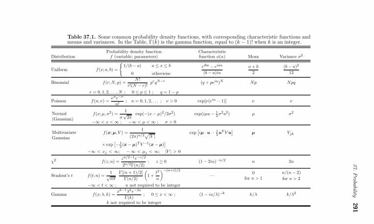
37.Pro
bability
291
Table 37.1. Some common probability density functions, with corresponding characteristic functions andmeans and variances. In the Table, Γ(k) is the gamma function, equal to (k − 1)! when k is an integer.
Probability density function CharacteristicDistribution f (variable; parameters) function φ(u) Mean Variance σ2
Uniform f(x; a, b) =
1/(b − a) a ≤ x ≤ b
0 otherwise
eibu − eiau
(b − a)iu
a + b
2
(b − a)2
12
Binomial f(r; N, p) =N !
r!(N − r)!prqN−r (q + peiu)N Np Npq
r = 0, 1, 2, . . . , N ; 0 ≤ p ≤ 1 ; q = 1 − p
Poisson f(n; ν) =νne−ν
n!; n = 0, 1, 2, . . . ; ν > 0 exp[ν(eiu − 1)] ν ν
Normal(Gaussian)
f(x; µ, σ2) =1
σ√
2πexp(−(x − µ)2/2σ2) exp(iµu − 1
2σ2u2) µ σ2
−∞ < x < ∞ ; −∞ < µ < ∞ ; σ > 0
MultivariateGaussian
f(x; µ, V ) =1
(2π)n/2√
|V |exp
[
iµ · u − 12uT V u
]
µ Vjk
× exp[
−12 (x − µ)T V −1(x − µ)
]
−∞ < xj < ∞; − ∞ < µj < ∞; |V | > 0
χ2 f(z; n) =zn/2−1e−z/2
2n/2Γ(n/2); z ≥ 0 (1 − 2iu)−n/2 n 2n
Student’s t f(t; n) =1√nπ
Γ[(n + 1)/2]
Γ(n/2)
(
1 +t2
n
)−(n+1)/2
—0
for n > 1
n/(n − 2)
for n > 2
−∞ < t < ∞ ; n not required to be integer
Gamma f(x; λ, k) =xk−1λke−λx
Γ(k); 0 ≤ x < ∞ ; (1 − iu/λ)−k k/λ k/λ2
k not required to be integer
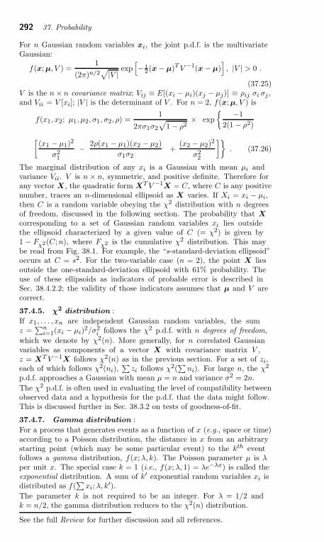
292 37. Probability
For n Gaussian random variables xi, the joint p.d.f. is the multivariateGaussian:
f(x; µ, V ) =1
(2π)n/2√
|V |exp
[
− 1
2(x − µ)T V −1(x − µ)
]
, |V | > 0 .
(37.25)V is the n × n covariance matrix; Vij ≡ E[(xi − µi)(xj − µj)] ≡ ρij σi σj ,and Vii = V [xi]; |V | is the determinant of V . For n = 2, f(x; µ, V ) is
f(x1, x2; µ1, µ2, σ1, σ2, ρ) =1
2πσ1σ2
√
1 − ρ2× exp
−1
2(1 − ρ2)
[
(x1 − µ1)2
σ21
− 2ρ(x1 − µ1)(x2 − µ2)
σ1σ2+
(x2 − µ2)2
σ22
]
. (37.26)
The marginal distribution of any xi is a Gaussian with mean µi andvariance Vii. V is n × n, symmetric, and positive definite. Therefore forany vector X, the quadratic form XT V −1X = C, where C is any positivenumber, traces an n-dimensional ellipsoid as X varies. If Xi = xi − µi,then C is a random variable obeying the χ2 distribution with n degreesof freedom, discussed in the following section. The probability that X
corresponding to a set of Gaussian random variables xi lies outsidethe ellipsoid characterized by a given value of C (= χ2) is given by1 − Fχ2(C; n), where Fχ2 is the cumulative χ2 distribution. This maybe read from Fig. 38.1. For example, the “s-standard-deviation ellipsoid”occurs at C = s2. For the two-variable case (n = 2), the point X liesoutside the one-standard-deviation ellipsoid with 61% probability. Theuse of these ellipsoids as indicators of probable error is described inSec. 38.4.2.2; the validity of those indicators assumes that µ and V arecorrect.
37.4.5. χ2distribution :
If x1, . . . , xn are independent Gaussian random variables, the sumz =
∑ni=1(xi − µi)
2/σ2i follows the χ2 p.d.f. with n degrees of freedom,
which we denote by χ2(n). More generally, for n correlated Gaussianvariables as components of a vector X with covariance matrix V ,z = XT V −1X follows χ2(n) as in the previous section. For a set of zi,each of which follows χ2(ni),
∑
zi follows χ2(∑
ni). For large n, the χ2
p.d.f. approaches a Gaussian with mean µ = n and variance σ2 = 2n.
The χ2 p.d.f. is often used in evaluating the level of compatibility betweenobserved data and a hypothesis for the p.d.f. that the data might follow.This is discussed further in Sec. 38.3.2 on tests of goodness-of-fit.
37.4.7. Gamma distribution :
For a process that generates events as a function of x (e.g., space or time)according to a Poisson distribution, the distance in x from an arbitrarystarting point (which may be some particular event) to the kth eventfollows a gamma distribution, f(x; λ, k). The Poisson parameter µ is λper unit x. The special case k = 1 (i.e., f(x; λ, 1) = λe−λx) is called theexponential distribution. A sum of k′ exponential random variables xi isdistributed as f(
∑
xi; λ, k′).
The parameter k is not required to be an integer. For λ = 1/2 andk = n/2, the gamma distribution reduces to the χ2(n) distribution.
See the full Review for further discussion and all references.
38. Statistics 293
38. STATISTICS
Revised September 2013 by G. Cowan (RHUL).
There are two main approaches to statistical inference, which wemay call frequentist and Bayesian. In frequentist statistics, probability isinterpreted as the frequency of the outcome of a repeatable experiment.The most important tools in this framework are parameter estimation,covered in Section 38.2, statistical tests, discussed in Section 38.3, andconfidence intervals, which are constructed so as to cover the true value ofa parameter with a specified probability, as described in Section 38.4.2.Note that in frequentist statistics one does not define a probability for ahypothesis or for the value of a parameter.
In Bayesian statistics, the interpretation of probability is more generaland includes degree of belief (called subjective probability). One can thenspeak of a probability density function (p.d.f.) for a parameter, whichexpresses one’s state of knowledge about where its true value lies. UsingBayes’ theorem (Eq. (37.4)), the prior degree of belief is updated by thedata from the experiment. Bayesian methods for interval estimation arediscussed in Sections 38.4.1 and 38.4.2.4.
Following common usage in physics, the word “error” is often used inthis chapter to mean “uncertainty.” More specifically it can indicate thesize of an interval as in “the standard error” or “error propagation,” wherethe term refers to the standard deviation of an estimator.
38.2. Parameter estimation
Here we review point estimation of parameters. An estimator θ (writtenwith a hat) is a function of the data used to estimate the value of theparameter θ.
38.2.1. Estimators for mean, variance, and median :
Suppose we have a set of n independent measurements, x1, . . . , xn, eachassumed to follow a p.d.f. with unknown mean µ and unknown varianceσ2. The measurements do not necessarily have to follow a Gaussiandistribution. Then
µ =1
n
n∑
i=1
xi (38.5)
σ2 =1
n − 1
n∑
i=1
(xi − µ)2 (38.6)
are unbiased estimators of µ and σ2. The variance of µ is σ2/n and the
variance of σ2 is
V[σ2
]=
1
n
(m4 − n − 3
n − 1σ4
), (38.7)
where m4 is the 4th central moment of x (see Eq. (37.8b)). For Gaussiandistributed xi, this becomes 2σ4/(n − 1) for any n ≥ 2, and for large n
the standard deviation of σ (the “error of the error”) is σ/√
2n. For anyn and Gaussian xi, µ is an efficient estimator for µ, and the estimators
µ and σ2 are uncorrelated. Otherwise the arithmetic mean (38.5) is notnecessarily the most efficient estimator.
If the xi have different, known variances σ2i , then the weighted average
µ =1
w
n∑
i=1
wixi , (38.8)
294 38. Statistics
where wi = 1/σ2i and w =
∑i wi, is an unbiased estimator for µ with a
smaller variance than an unweighted average. The standard deviation ofµ is 1/
√w.
38.2.2. The method of maximum likelihood :
Suppose we have a set of measured quantities x and the likelihoodL(θ) = P (x|θ) for a set of parameters θ = (θ1, . . . , θN ). The maximumlikelihood (ML) estimators for θ are defined as the values that give themaximum of L. Because of the properties of the logarithm, it is usuallyeasier to work with lnL, and since both are maximized for the sameparameter values θ, the ML estimators can be found by solving thelikelihood equations,
∂ lnL
∂θi= 0 , i = 1, . . . , N . (38.9)
In evaluating the likelihood function, it is important that anynormalization factors in the p.d.f. that involve θ be included.
The inverse V −1 of the covariance matrix Vij = cov[θi, θj ] for a set ofML estimators can be estimated by using
(V −1)ij = − ∂2 lnL
∂θi∂θj
∣∣∣∣θ
; (38.12)
for finite samples, however, Eq. (38.12) can result in an underestimateof the variances. In the large sample limit (or in a linear model withGaussian errors), L has a Gaussian form and lnL is (hyper)parabolic. Inthis case, it can be seen that a numerically equivalent way of determinings-standard-deviation errors is from the hypersurface defined by the θ′ suchthat
lnL(θ′) = lnLmax − s2/2 , (38.13)
where ln Lmax is the value of lnL at the solution point (compare withEq. (38.68)). The minimum and maximum values of θi on the hypersurfacethen give an approximate s-standard deviation confidence interval for θi(see Section 38.4.2.2).
38.2.3. The method of least squares :
The method of least squares (LS) coincides with the method of maximumlikelihood in the following special case. Consider a set of N independentmeasurements yi at known points xi. The measurement yi is assumedto be Gaussian distributed with mean µ(xi; θ) and known variance σ2
i .The goal is to construct estimators for the unknown parameters θ. Thelikelihood function contains the sum of squares
χ2(θ) = −2 lnL(θ) + constant =
N∑
i=1
(yi − µ(xi; θ))2
σ2i
. (38.19)
The parameter values that maximize L are the same as those whichminimize χ2.
The minimum of Equation (38.19) defines the least-squares estimators
θ for the more general case where the yi are not Gaussian distributedas long as they are independent. If they are not independent but ratherhave a covariance matrix Vij = cov[yi, yj ], then the LS estimators aredetermined by the minimum of
χ2(θ) = (y − µ(θ))T V −1(y − µ(θ)) , (38.20)
where y = (y1, . . . , yN ) is the (column) vector of measurements, µ(θ)is the corresponding vector of predicted values, and the superscript Tdenotes the transpose.
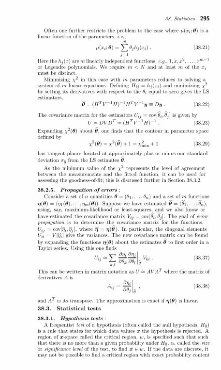
38. Statistics 295
Often one further restricts the problem to the case where µ(xi; θ) is alinear function of the parameters, i.e.,
µ(xi; θ) =m∑
j=1
θjhj(xi) . (38.21)
Here the hj(x) are m linearly independent functions, e.g., 1, x, x2, . . . , xm−1
or Legendre polynomials. We require m < N and at least m of the ximust be distinct.
Minimizing χ2 in this case with m parameters reduces to solving asystem of m linear equations. Defining Hij = hj(xi) and minimizing χ2
by setting its derivatives with respect to the θi equal to zero gives the LSestimators,
θ = (HT V −1H)−1HT V −1y ≡ Dy . (38.22)
The covariance matrix for the estimators Uij = cov[θi, θj ] is given by
U = DV DT = (HT V −1H)−1 . (38.23)
Expanding χ2(θ) about θ, one finds that the contour in parameter spacedefined by
χ2(θ) = χ2(θ) + 1 = χ2min + 1 (38.29)
has tangent planes located at approximately plus-or-minus-one standard
deviation σθ
from the LS estimates θ.
As the minimum value of the χ2 represents the level of agreementbetween the measurements and the fitted function, it can be used forassessing the goodness-of-fit; this is discussed further in Section 38.3.2.
38.2.5. Propagation of errors :Consider a set of n quantities θ = (θ1, . . . , θn) and a set of m functions
η(θ) = (η1(θ), . . . , ηm(θ)). Suppose we have estimated θ = (θ1, . . . , θn),using, say, maximum-likelihood or least-squares, and we also know or
have estimated the covariance matrix Vij = cov[θi, θj ]. The goal of errorpropagation is to determine the covariance matrix for the functions,
Uij = cov[ηi, ηj ], where η = η(θ ). In particular, the diagonal elementsUii = V [ηi] give the variances. The new covariance matrix can be found
by expanding the functions η(θ) about the estimates θ to first order in aTaylor series. Using this one finds
Uij ≈∑
k,l
∂ηi
∂θk
∂ηj
∂θl
∣∣∣∣θ
Vkl . (38.37)
This can be written in matrix notation as U ≈ AV AT where the matrix ofderivatives A is
Aij =∂ηi
∂θj
∣∣∣∣θ
, (38.38)
and AT is its transpose. The approximation is exact if η(θ) is linear.
38.3. Statistical tests
38.3.1. Hypothesis tests :A frequentist test of a hypothesis (often called the null hypothesis, H0)
is a rule that states for which data values x the hypothesis is rejected. Aregion of x-space called the critical region, w, is specified such that suchthat there is no more than a given probability under H0, α, called the sizeor significance level of the test, to find x ∈ w. If the data are discrete, itmay not be possible to find a critical region with exact probability content
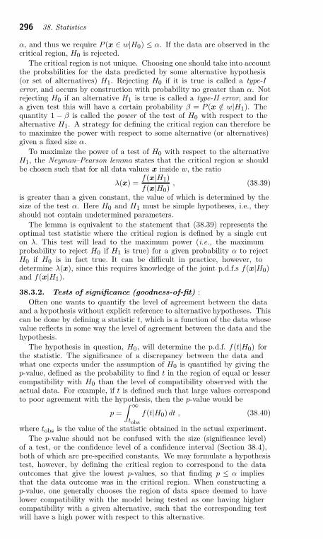
296 38. Statistics
α, and thus we require P (x ∈ w|H0) ≤ α. If the data are observed in thecritical region, H0 is rejected.
The critical region is not unique. Choosing one should take into accountthe probabilities for the data predicted by some alternative hypothesis(or set of alternatives) H1. Rejecting H0 if it is true is called a type-Ierror, and occurs by construction with probability no greater than α. Notrejecting H0 if an alternative H1 is true is called a type-II error, and fora given test this will have a certain probability β = P (x /∈ w|H1). Thequantity 1 − β is called the power of the test of H0 with respect to thealternative H1. A strategy for defining the critical region can therefore beto maximize the power with respect to some alternative (or alternatives)given a fixed size α.
To maximize the power of a test of H0 with respect to the alternativeH1, the Neyman–Pearson lemma states that the critical region w shouldbe chosen such that for all data values x inside w, the ratio
λ(x) =f(x|H1)
f(x|H0), (38.39)
is greater than a given constant, the value of which is determined by thesize of the test α. Here H0 and H1 must be simple hypotheses, i.e., theyshould not contain undetermined parameters.
The lemma is equivalent to the statement that (38.39) represents theoptimal test statistic where the critical region is defined by a single cuton λ. This test will lead to the maximum power (i.e., the maximumprobability to reject H0 if H1 is true) for a given probability α to rejectH0 if H0 is in fact true. It can be difficult in practice, however, todetermine λ(x), since this requires knowledge of the joint p.d.f.s f(x|H0)and f(x|H1).
38.3.2. Tests of significance (goodness-of-fit) :
Often one wants to quantify the level of agreement between the dataand a hypothesis without explicit reference to alternative hypotheses. Thiscan be done by defining a statistic t, which is a function of the data whosevalue reflects in some way the level of agreement between the data and thehypothesis.
The hypothesis in question, H0, will determine the p.d.f. f(t|H0) forthe statistic. The significance of a discrepancy between the data andwhat one expects under the assumption of H0 is quantified by giving thep-value, defined as the probability to find t in the region of equal or lessercompatibility with H0 than the level of compatibility observed with theactual data. For example, if t is defined such that large values correspondto poor agreement with the hypothesis, then the p-value would be
p =
∫∞
tobs
f(t|H0) dt , (38.40)
where tobs is the value of the statistic obtained in the actual experiment.
The p-value should not be confused with the size (significance level)of a test, or the confidence level of a confidence interval (Section 38.4),both of which are pre-specified constants. We may formulate a hypothesistest, however, by defining the critical region to correspond to the dataoutcomes that give the lowest p-values, so that finding p ≤ α impliesthat the data outcome was in the critical region. When constructing ap-value, one generally chooses the region of data space deemed to havelower compatibility with the model being tested as one having highercompatibility with a given alternative, such that the corresponding testwill have a high power with respect to this alternative.
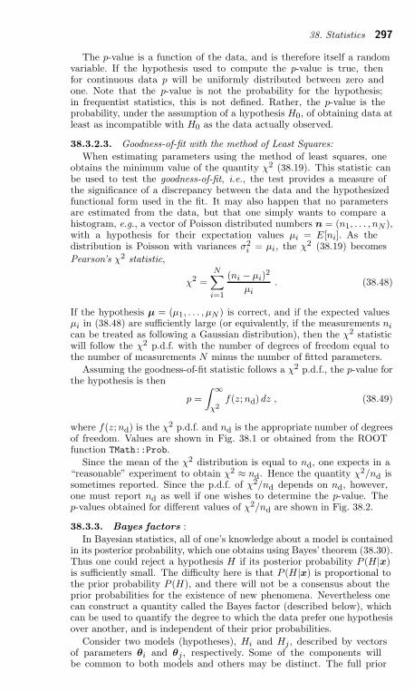
38. Statistics 297
The p-value is a function of the data, and is therefore itself a randomvariable. If the hypothesis used to compute the p-value is true, thenfor continuous data p will be uniformly distributed between zero andone. Note that the p-value is not the probability for the hypothesis;in frequentist statistics, this is not defined. Rather, the p-value is theprobability, under the assumption of a hypothesis H0, of obtaining data atleast as incompatible with H0 as the data actually observed.
38.3.2.3. Goodness-of-fit with the method of Least Squares:
When estimating parameters using the method of least squares, oneobtains the minimum value of the quantity χ2 (38.19). This statistic canbe used to test the goodness-of-fit, i.e., the test provides a measure ofthe significance of a discrepancy between the data and the hypothesizedfunctional form used in the fit. It may also happen that no parametersare estimated from the data, but that one simply wants to compare ahistogram, e.g., a vector of Poisson distributed numbers n = (n1, . . . , nN ),with a hypothesis for their expectation values µi = E[ni]. As thedistribution is Poisson with variances σ2
i = µi, the χ2 (38.19) becomes
Pearson’s χ2 statistic,
χ2 =
N∑
i=1
(ni − µi)2
µi. (38.48)
If the hypothesis µ = (µ1, . . . , µN ) is correct, and if the expected valuesµi in (38.48) are sufficiently large (or equivalently, if the measurements nican be treated as following a Gaussian distribution), then the χ2 statisticwill follow the χ2 p.d.f. with the number of degrees of freedom equal tothe number of measurements N minus the number of fitted parameters.
Assuming the goodness-of-fit statistic follows a χ2 p.d.f., the p-value forthe hypothesis is then
p =
∫∞
χ2f(z; nd) dz , (38.49)
where f(z; nd) is the χ2 p.d.f. and nd is the appropriate number of degreesof freedom. Values are shown in Fig. 38.1 or obtained from the ROOTfunction TMath::Prob.
Since the mean of the χ2 distribution is equal to nd, one expects in a“reasonable” experiment to obtain χ2 ≈ nd. Hence the quantity χ2/nd issometimes reported. Since the p.d.f. of χ2/nd depends on nd, however,one must report nd as well if one wishes to determine the p-value. Thep-values obtained for different values of χ2/nd are shown in Fig. 38.2.
38.3.3. Bayes factors :
In Bayesian statistics, all of one’s knowledge about a model is containedin its posterior probability, which one obtains using Bayes’ theorem (38.30).Thus one could reject a hypothesis H if its posterior probability P (H |x)is sufficiently small. The difficulty here is that P (H |x) is proportional tothe prior probability P (H), and there will not be a consensus about theprior probabilities for the existence of new phenomena. Nevertheless onecan construct a quantity called the Bayes factor (described below), whichcan be used to quantify the degree to which the data prefer one hypothesisover another, and is independent of their prior probabilities.
Consider two models (hypotheses), Hi and Hj , described by vectorsof parameters θi and θj , respectively. Some of the components willbe common to both models and others may be distinct. The full prior
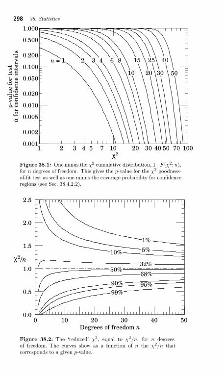
298 38. Statistics
1 2 3 4 5 7 10 20 30 40 50 70 1000.001
0.002
0.005
0.010
0.020
0.050
0.100
0.200
0.500
1.000
p-v
alu
e f
or
test
α fo
r co
nfi
den
ce i
nte
rvals
3 42 6 8
10
15
20
25
30
40
50
n = 1
χ2
Figure 38.1: One minus the χ2 cumulative distribution, 1−F (χ2; n),for n degrees of freedom. This gives the p-value for the χ2 goodness-of-fit test as well as one minus the coverage probability for confidenceregions (see Sec. 38.4.2.2).
0 10 20 30 40 500.0
0.5
1.0
1.5
2.0
2.5
Degrees of freedom n
50%
10%
90%
99%
95%
68%
32%
5%
1%
χ2/n
Figure 38.2: The ‘reduced’ χ2, equal to χ2/n, for n degreesof freedom. The curves show as a function of n the χ2/n thatcorresponds to a given p-value.
38. Statistics 299
probability for each model can be written in the form
π(Hi, θi) = P (Hi)π(θi|Hi) . (38.50)
Here P (Hi) is the overall prior probability for Hi, and π(θi|Hi) isthe normalized p.d.f. of its parameters. For each model, the posteriorprobability is found using Bayes’ theorem,
P (Hi|x) =
∫P (x|θi, Hi)P (Hi)π(θi|Hi) dθi
P (x), (38.51)
where the integration is carried out over the internal parameters θi of themodel. The ratio of posterior probabilities for the models is therefore
P (Hi|x)
P (Hj |x)=
∫P (x|θi, Hi)π(θi|Hi) dθi∫P (x|θj , Hj)π(θj |Hj) dθj
P (Hi)
P (Hj). (38.52)
The Bayes factor is defined as
Bij =
∫P (x|θi, Hi)π(θi|Hi) dθi∫P (x|θj , Hj)π(θj |Hj) dθj
. (38.53)
This gives what the ratio of posterior probabilities for models i and jwould be if the overall prior probabilities for the two models were equal.If the models have no nuisance parameters, i.e., no internal parametersdescribed by priors, then the Bayes factor is simply the likelihood ratio.The Bayes factor therefore shows by how much the probability ratio ofmodel i to model j changes in the light of the data, and thus can beviewed as a numerical measure of evidence supplied by the data in favourof one hypothesis over the other.
Although the Bayes factor is by construction independent of the overallprior probabilities P (Hi) and P (Hj), it does require priors for all internalparameters of a model, i.e., one needs the functions π(θi|Hi) and π(θj |Hj).In a Bayesian analysis where one is only interested in the posterior p.d.f.of a parameter, it may be acceptable to take an unnormalizable functionfor the prior (an improper prior) as long as the product of likelihood andprior can be normalized. But improper priors are only defined up to anarbitrary multiplicative constant, and so the Bayes factor would depend onthis constant. Furthermore, although the range of a constant normalizedprior is unimportant for parameter determination (provided it is widerthan the likelihood), this is not so for the Bayes factor when such a prioris used for only one of the hypotheses. So to compute a Bayes factor, allinternal parameters must be described by normalized priors that representmeaningful probabilities over the entire range where they are defined.
38.4. Intervals and limits
When the goal of an experiment is to determine a parameter θ,the result is usually expressed by quoting, in addition to the pointestimate, some sort of interval which reflects the statistical precision of themeasurement. In the simplest case, this can be given by the parameter’s
estimated value θ plus or minus an estimate of the standard deviation of
θ, σθ. If, however, the p.d.f. of the estimator is not Gaussian or if there
are physical boundaries on the possible values of the parameter, thenone usually quotes instead an interval according to one of the proceduresdescribed below.
38.4.1. Bayesian intervals :
As described in Sec. 38.2.4, a Bayesian posterior probability may beused to determine regions that will have a given probability of containingthe true value of a parameter. In the single parameter case, for example, aninterval (called a Bayesian or credible interval) [θlo, θup] can be determined
300 38. Statistics
which contains a given fraction 1 − α of the posterior probability, i.e.,
1 − α =
∫ θup
θlo
p(θ|x) dθ . (38.55)
Sometimes an upper or lower limit is desired, i.e., θlo or θup can be set toa physical boundary or to plus or minus infinity. In other cases, one mightbe interested in the set of θ values for which p(θ|x) is higher than forany θ not belonging to the set, which may constitute a single interval ora set of disjoint regions; these are called highest posterior density (HPD)intervals. Note that HPD intervals are not invariant under a nonlineartransformation of the parameter.
If a parameter is constrained to be non-negative, then the prior p.d.f.can simply be set to zero for negative values. An important example isthe case of a Poisson variable n, which counts signal events with unknownmean s, as well as background with mean b, assumed known. For thesignal mean s, one often uses the prior
π(s) =
0 s < 01 s ≥ 0
. (38.56)
For example, to obtain an upper limit on s, one may proceed as follows.The likelihood for s is given by the Poisson distribution for n with means + b,
P (n|s) =(s + b)n
n!e−(s+b) , (38.57)
along with the prior (38.56) in (38.30) gives the posterior density for s.An upper limit sup at confidence level (or here, rather, credibility level)1 − α can be obtained by requiring
1 − α =
∫ sup
−∞
p(s|n)ds =
∫ sup
−∞P (n|s)π(s) ds∫
∞
−∞P (n|s)π(s) ds
, (38.58)
where the lower limit of integration is effectively zero because of the cut-offin π(s). By relating the integrals in Eq. (38.58) to incomplete gammafunctions, the solution for the upper limit is found to be
sup = 12F−1
χ2 [p, 2(n + 1)] − b , (38.59)
where F−1χ2 is the quantile of the χ2 distribution (inverse of the cumulative
distribution). Here the quantity p is
p = 1 − α(Fχ2 [2b, 2(n + 1)]
), (38.60)
where Fχ2 is the cumulative χ2 distribution. For both Fχ2 and F−1χ2
above, the argument 2(n + 1) gives the number of degrees of freedom. Forthe special case of b = 0, the limit reduces to
sup = 12F−1
χ2 (1 − α; 2(n + 1)) . (38.61)
It happens that for the case of b = 0, the upper limit from Eq. (38.61)coincides numerically with the frequentist upper limit discussed inSection 38.4.2.3. Values for 1 − α = 0.9 and 0.95 are given by the valuesµup in Table 38.3.
38.4.2. Frequentist confidence intervals :
38.4.2.1. The Neyman construction for confidence intervals:
Consider a p.d.f. f(x; θ) where x represents the outcome of theexperiment and θ is the unknown parameter for which we want toconstruct a confidence interval. The variable x could (and often does)represent an estimator for θ. Using f(x; θ), we can find for a pre-specified
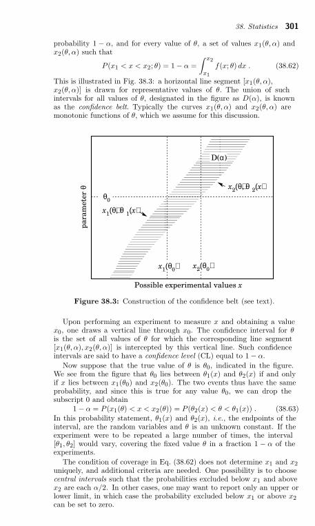
38. Statistics 301
probability 1 − α, and for every value of θ, a set of values x1(θ, α) andx2(θ, α) such that
P (x1 < x < x2; θ) = 1 − α =
∫ x2
x1
f(x; θ) dx . (38.62)
This is illustrated in Fig. 38.3: a horizontal line segment [x1(θ, α),x2(θ, α)] is drawn for representative values of θ. The union of suchintervals for all values of θ, designated in the figure as D(α), is knownas the confidence belt. Typically the curves x1(θ, α) and x2(θ, α) aremonotonic functions of θ, which we assume for this discussion.
Possible experimental values x
pa
ram
ete
r θ x
2(θ), θ
2(x)
x1(θ), θ
1(x)
x1(θ
0) x
2(θ
0)
D(α)
θ0
Figure 38.3: Construction of the confidence belt (see text).
Upon performing an experiment to measure x and obtaining a valuex0, one draws a vertical line through x0. The confidence interval for θis the set of all values of θ for which the corresponding line segment[x1(θ, α), x2(θ, α)] is intercepted by this vertical line. Such confidenceintervals are said to have a confidence level (CL) equal to 1 − α.
Now suppose that the true value of θ is θ0, indicated in the figure.We see from the figure that θ0 lies between θ1(x) and θ2(x) if and onlyif x lies between x1(θ0) and x2(θ0). The two events thus have the sameprobability, and since this is true for any value θ0, we can drop thesubscript 0 and obtain
1 − α = P (x1(θ) < x < x2(θ)) = P (θ2(x) < θ < θ1(x)) . (38.63)
In this probability statement, θ1(x) and θ2(x), i.e., the endpoints of theinterval, are the random variables and θ is an unknown constant. If theexperiment were to be repeated a large number of times, the interval[θ1, θ2] would vary, covering the fixed value θ in a fraction 1 − α of theexperiments.
The condition of coverage in Eq. (38.62) does not determine x1 and x2uniquely, and additional criteria are needed. One possibility is to choosecentral intervals such that the probabilities excluded below x1 and abovex2 are each α/2. In other cases, one may want to report only an upper orlower limit, in which case the probability excluded below x1 or above x2can be set to zero.
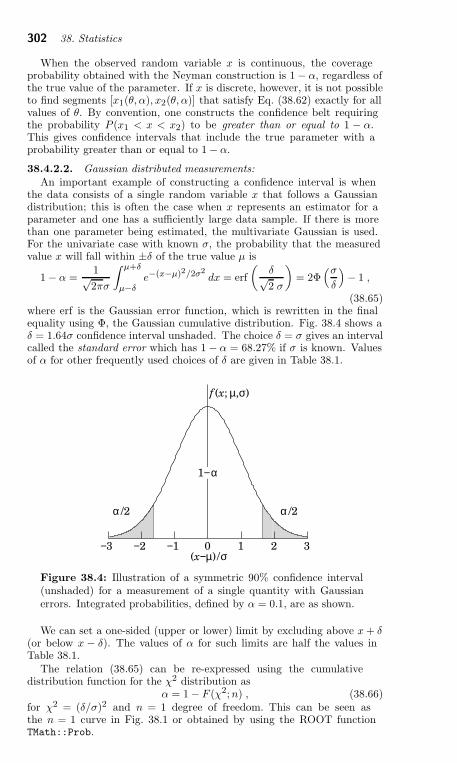
302 38. Statistics
When the observed random variable x is continuous, the coverageprobability obtained with the Neyman construction is 1 − α, regardless ofthe true value of the parameter. If x is discrete, however, it is not possibleto find segments [x1(θ, α), x2(θ, α)] that satisfy Eq. (38.62) exactly for allvalues of θ. By convention, one constructs the confidence belt requiringthe probability P (x1 < x < x2) to be greater than or equal to 1 − α.This gives confidence intervals that include the true parameter with aprobability greater than or equal to 1 − α.
38.4.2.2. Gaussian distributed measurements:
An important example of constructing a confidence interval is whenthe data consists of a single random variable x that follows a Gaussiandistribution; this is often the case when x represents an estimator for aparameter and one has a sufficiently large data sample. If there is morethan one parameter being estimated, the multivariate Gaussian is used.For the univariate case with known σ, the probability that the measuredvalue x will fall within ±δ of the true value µ is
1 − α =1√2πσ
∫ µ+δ
µ−δe−(x−µ)2/2σ2
dx = erf
(δ√2 σ
)= 2Φ
(σ
δ
)− 1 ,
(38.65)where erf is the Gaussian error function, which is rewritten in the finalequality using Φ, the Gaussian cumulative distribution. Fig. 38.4 shows aδ = 1.64σ confidence interval unshaded. The choice δ = σ gives an intervalcalled the standard error which has 1 − α = 68.27% if σ is known. Valuesof α for other frequently used choices of δ are given in Table 38.1.
−3 −2 −1 0 1 2 3
f (x; µ,σ)
α /2α /2
(x−µ) /σ
1−α
Figure 38.4: Illustration of a symmetric 90% confidence interval(unshaded) for a measurement of a single quantity with Gaussianerrors. Integrated probabilities, defined by α = 0.1, are as shown.
We can set a one-sided (upper or lower) limit by excluding above x + δ(or below x − δ). The values of α for such limits are half the values inTable 38.1.
The relation (38.65) can be re-expressed using the cumulativedistribution function for the χ2 distribution as
α = 1 − F (χ2; n) , (38.66)for χ2 = (δ/σ)2 and n = 1 degree of freedom. This can be seen asthe n = 1 curve in Fig. 38.1 or obtained by using the ROOT functionTMath::Prob.
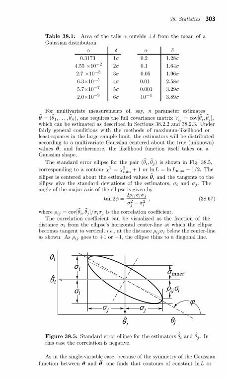
38. Statistics 303
Table 38.1: Area of the tails α outside ±δ from the mean of aGaussian distribution.
α δ α δ
0.3173 1σ 0.2 1.28σ
4.55 ×10⁻² 2σ 0.1 1.64σ
2.7 ×10⁻³ 3σ 0.05 1.96σ
6.3×10⁻⁵ 4σ 0.01 2.58σ
5.7×10⁻⁷ 5σ 0.001 3.29σ
2.0×10⁻⁹ 6σ 10−4 3.89σ
For multivariate measurements of, say, n parameter estimates
θ = (θ1, . . . , θn), one requires the full covariance matrix Vij = cov[θi, θj ],which can be estimated as described in Sections 38.2.2 and 38.2.3. Underfairly general conditions with the methods of maximum-likelihood orleast-squares in the large sample limit, the estimators will be distributedaccording to a multivariate Gaussian centered about the true (unknown)values θ, and furthermore, the likelihood function itself takes on aGaussian shape.
The standard error ellipse for the pair (θi, θj) is shown in Fig. 38.5,
corresponding to a contour χ2 = χ2min + 1 or lnL = lnLmax − 1/2. The
ellipse is centered about the estimated values θ, and the tangents to theellipse give the standard deviations of the estimators, σi and σj . Theangle of the major axis of the ellipse is given by
tan 2φ =2ρijσiσj
σ2j − σ2
i
, (38.67)
where ρij = cov[θi, θj ]/σiσj is the correlation coefficient.The correlation coefficient can be visualized as the fraction of the
distance σi from the ellipse’s horizontal center-line at which the ellipsebecomes tangent to vertical, i.e., at the distance ρijσi below the center-lineas shown. As ρij goes to +1 or −1, the ellipse thins to a diagonal line.
θ i
φ
θ i
jσ
θj
iσ
jσ
iσ
^
θ j^
ij iρ σ
innerσ
Figure 38.5: Standard error ellipse for the estimators θi and θj . Inthis case the correlation is negative.
As in the single-variable case, because of the symmetry of the Gaussian
function between θ and θ, one finds that contours of constant lnL or
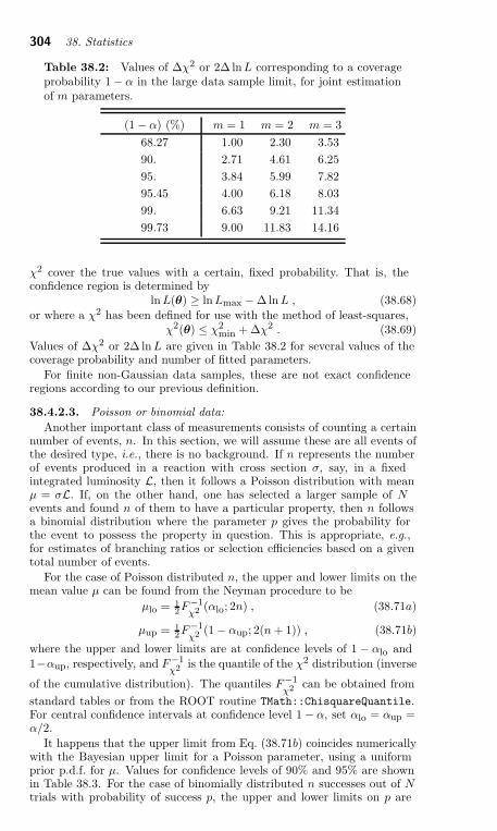
304 38. Statistics
Table 38.2: Values of ∆χ2 or 2∆ lnL corresponding to a coverageprobability 1 − α in the large data sample limit, for joint estimationof m parameters.
(1 − α) (%) m = 1 m = 2 m = 3
68.27 1.00 2.30 3.53
90. 2.71 4.61 6.25
95. 3.84 5.99 7.82
95.45 4.00 6.18 8.03
99. 6.63 9.21 11.34
99.73 9.00 11.83 14.16
χ2 cover the true values with a certain, fixed probability. That is, theconfidence region is determined by
lnL(θ) ≥ lnLmax − ∆ ln L , (38.68)
or where a χ2 has been defined for use with the method of least-squares,χ2(θ) ≤ χ2
min + ∆χ2 . (38.69)
Values of ∆χ2 or 2∆ lnL are given in Table 38.2 for several values of thecoverage probability and number of fitted parameters.
For finite non-Gaussian data samples, these are not exact confidenceregions according to our previous definition.
38.4.2.3. Poisson or binomial data:
Another important class of measurements consists of counting a certainnumber of events, n. In this section, we will assume these are all events ofthe desired type, i.e., there is no background. If n represents the numberof events produced in a reaction with cross section σ, say, in a fixedintegrated luminosity L, then it follows a Poisson distribution with meanµ = σL. If, on the other hand, one has selected a larger sample of Nevents and found n of them to have a particular property, then n followsa binomial distribution where the parameter p gives the probability forthe event to possess the property in question. This is appropriate, e.g.,for estimates of branching ratios or selection efficiencies based on a giventotal number of events.
For the case of Poisson distributed n, the upper and lower limits on themean value µ can be found from the Neyman procedure to be
µlo = 12F−1
χ2 (αlo; 2n) , (38.71a)
µup = 12F−1
χ2 (1 − αup; 2(n + 1)) , (38.71b)
where the upper and lower limits are at confidence levels of 1 − αlo and
1−αup, respectively, and F−1χ2 is the quantile of the χ2 distribution (inverse
of the cumulative distribution). The quantiles F−1χ2 can be obtained from
standard tables or from the ROOT routine TMath::ChisquareQuantile.For central confidence intervals at confidence level 1 − α, set αlo = αup =α/2.
It happens that the upper limit from Eq. (38.71b) coincides numericallywith the Bayesian upper limit for a Poisson parameter, using a uniformprior p.d.f. for µ. Values for confidence levels of 90% and 95% are shownin Table 38.3. For the case of binomially distributed n successes out of Ntrials with probability of success p, the upper and lower limits on p are
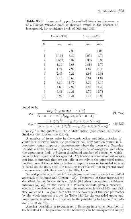
38. Statistics 305
Table 38.3: Lower and upper (one-sided) limits for the mean µof a Poisson variable given n observed events in the absence ofbackground, for confidence levels of 90% and 95%.
1 − α =90% 1 − α =95%
n µlo µup µlo µup
0 – 2.30 – 3.00
1 0.105 3.89 0.051 4.74
2 0.532 5.32 0.355 6.30
3 1.10 6.68 0.818 7.75
4 1.74 7.99 1.37 9.15
5 2.43 9.27 1.97 10.51
6 3.15 10.53 2.61 11.84
7 3.89 11.77 3.29 13.15
8 4.66 12.99 3.98 14.43
9 5.43 14.21 4.70 15.71
10 6.22 15.41 5.43 16.96
found to be
plo =nF−1
F [αlo; 2n, 2(N − n + 1)]
N − n + 1 + nF−1F [αlo; 2n, 2(N − n + 1)]
, (38.72a)
pup =(n + 1)F−1
F [1 − αup; 2(n + 1), 2(N − n)]
(N − n) + (n + 1)F−1F [1 − αup; 2(n + 1), 2(N − n)]
. (38.72b)
Here F−1F is the quantile of the F distribution (also called the Fisher–
Snedecor distribution; see Ref. 4).
A number of issues arise in the construction and interpretation ofconfidence intervals when the parameter can only take on values in arestricted range. Important examples are where the mean of a Gaussianvariable is constrained on physical grounds to be non-negative and wherethe experiment finds a Poisson-distributed number of events, n, whichincludes both signal and background. Application of some standard recipescan lead to intervals that are partially or entirely in the unphysical region.Furthermore, if the decision whether to report a one- or two-sided intervalis based on the data, then the resulting intervals will not in general coverthe parameter with the stated probability 1 − α.
Several problems with such intervals are overcome by using the unifiedapproach of Feldman and Cousins [33]. Properties of these intervals aredescribed further in the Review. Table 38.4 gives the unified confidenceintervals [µ1, µ2] for the mean of a Poisson variable given n observedevents in the absence of background, for confidence levels of 90% and 95%.The values of 1 − α given here refer to the coverage of the true parameterby the whole interval [µ1, µ2]. In Table 38.3 for the one-sided upper andlower limits, however, 1−α referred to the probability to have individuallyµup ≥ µ or µlo ≤ µ.
Another possibility is to construct a Bayesian interval as described inSection 38.4.1. The presence of the boundary can be incorporated simply
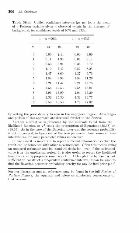
306 38. Statistics
Table 38.4: Unified confidence intervals [µ1, µ2] for a the meanof a Poisson variable given n observed events in the absence ofbackground, for confidence levels of 90% and 95%.
1 − α =90% 1 − α =95%
n µ1 µ2 µ1 µ2
0 0.00 2.44 0.00 3.09
1 0.11 4.36 0.05 5.14
2 0.53 5.91 0.36 6.72
3 1.10 7.42 0.82 8.25
4 1.47 8.60 1.37 9.76
5 1.84 9.99 1.84 11.26
6 2.21 11.47 2.21 12.75
7 3.56 12.53 2.58 13.81
8 3.96 13.99 2.94 15.29
9 4.36 15.30 4.36 16.77
10 5.50 16.50 4.75 17.82
by setting the prior density to zero in the unphysical region. Advantagesand pitfalls of this approach are discussed further in the Review.
Another alternative is presented by the intervals found from thelikelihood function or χ2 using the prescription of Equations (38.68) or(38.69). As in the case of the Bayesian intervals, the coverage probabilityis not, in general, independent of the true parameter. Furthermore, theseintervals can for some parameter values undercover.
In any case it is important to report sufficient information so that theresult can be combined with other measurements. Often this means givingan unbiased estimator and its standard deviation, even if the estimatedvalue is in the unphysical region. It is also useful to report the likelihoodfunction or an appropriate summary of it. Although this by itself is notsufficient to construct a frequentist confidence interval, it can be used tofind the Bayesian posterior probability density for any desired prior p.d.f.
Further discussion and all references may be found in the full Review ofParticle Physics; the equation and reference numbering corresponds tothat version.
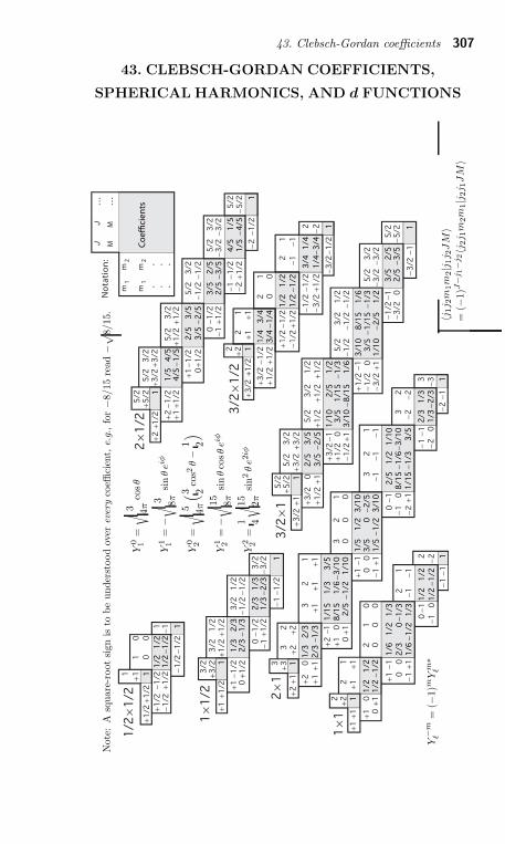
43. Clebsch-Gordan coefficients 307
43. CLEBSCH-GORDAN COEFFICIENTS,
SPHERICAL HARMONICS, AND d FUNCTIONSN
ote
:A
square
-root
sign
isto
be
under
stood
over
every
coeffi
cien
t,e.g
.,fo
r−
8/15
read−
√
8/15.
Y0 1
=
√
3 4π
cosθ
Y1 1
=−
√
3 8π
sin
θei
φ
Y0 2
=
√
5 4π
(
3 2co
s2θ−
1 2
)
Y1 2
=−
√
15
8π
sin
θco
sθei
φ
Y2 2
=1 4
√
15
2π
sin2θ
e2iφ
Y−
mℓ
=(−
1)m
Ym∗
ℓ
〈j1j 2
m1m
2|j 1
j 2JM
〉=
(−1)J
−j 1−
j 2〈j
2j 1
m2m
1|j 2
j 1JM
〉
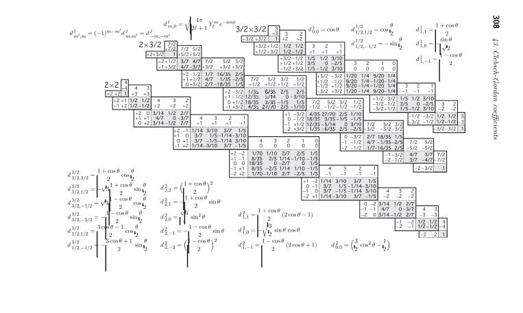
308
43.Clebsc
h-G
ord
an
coeffi
cie
nts
d ℓm,0 =
√
4π
2ℓ + 1Y m
ℓ e−imφ
djm′,m
= (−1)m−m′
djm,m′
= dj−m,−m′
d 10,0 = cos θ d
1/2
1/2,1/2= cos
θ
2
d1/2
1/2,−1/2= − sin
θ
2
d 11,1 =
1 + cos θ
2
d 11,0 = − sin θ√
2
d 11,−1
=1 − cos θ
2
d3/2
3/2,3/2=
1 + cos θ
2cos
θ
2
d3/2
3/2,1/2= −
√31 + cos θ
2sin
θ
2
d3/2
3/2,−1/2=
√31 − cos θ
2cos
θ
2
d3/2
3/2,−3/2= −1 − cos θ
2sin
θ
2
d3/2
1/2,1/2=
3 cos θ − 1
2cos
θ
2
d3/2
1/2,−1/2= −3 cos θ + 1
2sin
θ
2
d 22,2 =
(1 + cos θ
2
)
2
d 22,1 = −1 + cos θ
2sin θ
d 22,0 =
√6
4sin2 θ
d 22,−1
= −1 − cos θ
2sin θ
d 22,−2
=(1 − cos θ
2
)
2
d 21,1 =
1 + cos θ
2(2 cos θ − 1)
d 21,0 = −
√
3
2sin θ cos θ
d 21,−1
=1 − cos θ
2(2 cos θ + 1) d 2
0,0 =(3
2cos2 θ − 1
2
)
46. Kinematics 309
46. KINEMATICS
Revised January 2000 by J.D. Jackson (LBNL) and June 2008 by D.R.Tovey (Sheffield).
Throughout this section units are used in which ~ = c = 1. The followingconversions are useful: ~c = 197.3 MeV fm, (~c)2 = 0.3894 (GeV)2 mb.
46.1. Lorentz transformations
The energy E and 3-momentum p of a particle of mass m form a4-vector p = (E,p) whose square p2 ≡ E2 − |p|2 = m2. The velocity ofthe particle is β = p/E. The energy and momentum (E∗,p∗) viewed froma frame moving with velocity βf are given by
(
E∗
p∗‖
)
=
(
γf −γfβf−γfβf γf
) (
Ep‖
)
, p∗T
= pT
, (46.1)
where γf = (1−β2f )−1/2 and p
T(p‖) are the components of p perpendicular
(parallel) to βf . Other 4-vectors, such as the space-time coordinates ofevents, of course transform in the same way. The scalar product of two4-momenta p1 · p2 = E1E2 − p1 · p2 is invariant (frame independent).
46.2. Center-of-mass energy and momentum
In the collision of two particles of masses m1 and m2 the totalcenter-of-mass energy can be expressed in the Lorentz-invariant form
Ecm =[
(E1 + E2)2 − (p1 + p2)
2]1/2
,
=[
m21 + m2
2 + 2E1E2(1 − β1β2 cos θ)]1/2
, (46.2)
where θ is the angle between the particles. In the frame where one particle(of mass m2) is at rest (lab frame),
Ecm = (m21 + m2
2 + 2E1 lab m2)1/2 . (46.3)
The velocity of the center-of-mass in the lab frame is
βcm = plab/(E1 lab + m2) , (46.4)
where plab ≡ p1 lab and
γcm = (E1 lab + m2)/Ecm . (46.5)
The c.m. momenta of particles 1 and 2 are of magnitude
pcm = plabm2
Ecm. (46.6)
For example, if a 0.80 GeV/c kaon beam is incident on a proton target,the center of mass energy is 1.699 GeV and the center of mass momentumof either particle is 0.442 GeV/c. It is also useful to note that
Ecm dEcm = m2 dE1 lab = m2 β1 lab dplab . (46.7)
46.3. Lorentz-invariant amplitudes
The matrix elements for a scattering or decay process are written interms of an invariant amplitude −iM . As an example, the S-matrix for2 → 2 scattering is related to M by
〈p′1p′2 |S| p1p2〉 = I − i(2π)4 δ4(p1 + p2 − p′1 − p′2)
× M (p1, p2; p′1, p′2)
(2E1)1/2 (2E2)1/2 (2E′1)
1/2 (2E′2)
1/2. (46.8)
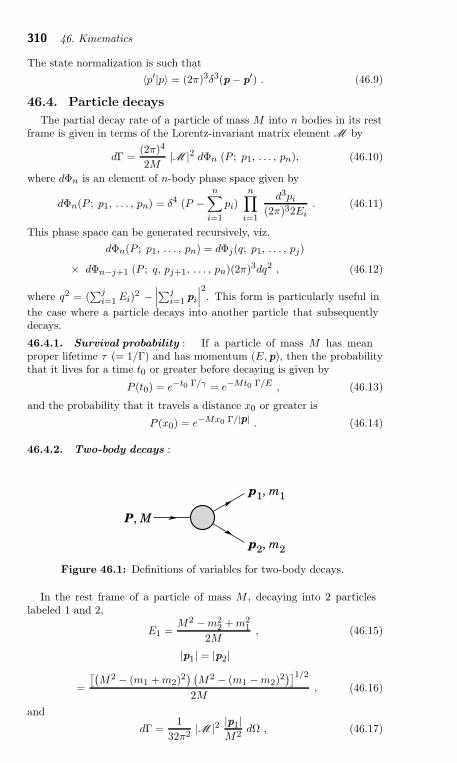
310 46. Kinematics
The state normalization is such that
〈p′|p〉 = (2π)3δ3(p− p′) . (46.9)
46.4. Particle decays
The partial decay rate of a particle of mass M into n bodies in its restframe is given in terms of the Lorentz-invariant matrix element M by
dΓ =(2π)4
2M|M |2 dΦn (P ; p1, . . . , pn), (46.10)
where dΦn is an element of n-body phase space given by
dΦn(P ; p1, . . . , pn) = δ4 (P −n
∑
i=1
pi)
n∏
i=1
d3pi
(2π)32Ei. (46.11)
This phase space can be generated recursively, viz.
dΦn(P ; p1, . . . , pn) = dΦj(q; p1, . . . , pj)
× dΦn−j+1 (P ; q, pj+1, . . . , pn)(2π)3dq2 , (46.12)
where q2 = (∑j
i=1 Ei)2 −
∣
∣
∣
∑ji=1 pi
∣
∣
∣
2. This form is particularly useful in
the case where a particle decays into another particle that subsequentlydecays.
46.4.1. Survival probability : If a particle of mass M has meanproper lifetime τ (= 1/Γ) and has momentum (E,p), then the probabilitythat it lives for a time t0 or greater before decaying is given by
P (t0) = e−t0 Γ/γ = e−Mt0 Γ/E , (46.13)
and the probability that it travels a distance x0 or greater is
P (x0) = e−Mx0 Γ/|p| . (46.14)
46.4.2. Two-body decays :
p1, m1
p2, m2
P, M
Figure 46.1: Definitions of variables for two-body decays.
In the rest frame of a particle of mass M , decaying into 2 particleslabeled 1 and 2,
E1 =M2 − m2
2 + m21
2M, (46.15)
|p1| = |p2|
=
[(
M2 − (m1 + m2)2) (
M2 − (m1 − m2)2)]1/2
2M, (46.16)
and
dΓ =1
32π2|M |2 |p1|
M2dΩ , (46.17)
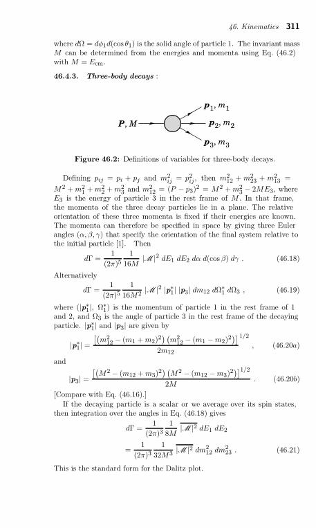
46. Kinematics 311
where dΩ = dφ1d(cos θ1) is the solid angle of particle 1. The invariant massM can be determined from the energies and momenta using Eq. (46.2)with M = Ecm.
46.4.3. Three-body decays :
p1, m1
p3, m3
P, M p2, m2
Figure 46.2: Definitions of variables for three-body decays.
Defining pij = pi + pj and m2ij = p2
ij , then m212 + m2
23 + m213 =
M2 + m21 + m2
2 + m23 and m2
12 = (P − p3)2 = M2 + m2
3 − 2ME3, whereE3 is the energy of particle 3 in the rest frame of M . In that frame,the momenta of the three decay particles lie in a plane. The relativeorientation of these three momenta is fixed if their energies are known.The momenta can therefore be specified in space by giving three Eulerangles (α, β, γ) that specify the orientation of the final system relative tothe initial particle [1]. Then
dΓ =1
(2π)51
16M|M |2 dE1 dE2 dα d(cos β) dγ . (46.18)
Alternatively
dΓ =1
(2π)51
16M2|M |2 |p∗1| |p3| dm12 dΩ∗
1 dΩ3 , (46.19)
where (|p∗1|, Ω∗1) is the momentum of particle 1 in the rest frame of 1
and 2, and Ω3 is the angle of particle 3 in the rest frame of the decayingparticle. |p∗1| and |p3| are given by
|p∗1| =
[(
m212 − (m1 + m2)
2) (
m212 − (m1 − m2)
2)]
2m12
1/2
, (46.20a)
and
|p3| =
[(
M2 − (m12 + m3)2) (
M2 − (m12 − m3)2)]1/2
2M. (46.20b)
[Compare with Eq. (46.16).]
If the decaying particle is a scalar or we average over its spin states,then integration over the angles in Eq. (46.18) gives
dΓ =1
(2π)31
8M|M |2 dE1 dE2
=1
(2π)31
32M3 |M |2 dm212 dm2
23 . (46.21)
This is the standard form for the Dalitz plot.
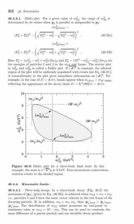
312 46. Kinematics
46.4.3.1. Dalitz plot: For a given value of m212, the range of m2
23 isdetermined by its values when p2 is parallel or antiparallel to p3:
(m223)max =
(E∗2 + E∗
3 )2 −(
√
E∗22 − m2
2 −√
E∗23 − m2
3
)2
, (46.22a)
(m223)min =
(E∗2 + E∗
3 )2 −(
√
E∗22 − m2
2 +√
E∗23 − m2
3
)2
. (46.22b)
Here E∗2 = (m2
12 − m21 + m2
2)/2m12 and E∗3 = (M2 −m2
12 −m23)/2m12 are
the energies of particles 2 and 3 in the m12 rest frame. The scatter plotin m2
12 and m223 is called a Dalitz plot. If |M |2 is constant, the allowed
region of the plot will be uniformly populated with events [see Eq. (46.21)].A nonuniformity in the plot gives immediate information on |M |2. Forexample, in the case of D → Kππ, bands appear when m(Kπ) = mK∗(892),
reflecting the appearance of the decay chain D → K∗(892)π → Kππ.
(m23)max
0 1 2 3 4 5 0
2
4
6
8
10
m12 (GeV2)
m2
3
(GeV
2)
(m1+m2)2
(M−m3)2
(M−m1)2
(m2+m3)2
(m23)min2
2
2
2
Figure 46.3: Dalitz plot for a three-body final state. In thisexample, the state is π+K0p at 3 GeV. Four-momentum conservationrestricts events to the shaded region.
46.4.4. Kinematic limits :
46.4.4.1. Three-body decays: In a three-body decay (Fig. 46.2) themaximum of |p3|, [given by Eq. (46.20)], is achieved when m12 = m1 +m2,i.e., particles 1 and 2 have the same vector velocity in the rest frame of thedecaying particle. If, in addition, m3 > m1, m2, then |p
3|max > |p
1|max,
|p2|max. The distribution of m12 values possesses an end-point or
maximum value at m12 = M − m3. This can be used to constrain themass difference of a parent particle and one invisible decay product.
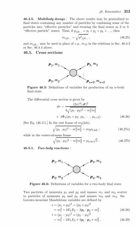
46. Kinematics 313
46.4.5. Multibody decays : The above results may be generalized tofinal states containing any number of particles by combining some of theparticles into “effective particles” and treating the final states as 2 or 3“effective particle” states. Thus, if pijk... = pi + pj + pk + . . ., then
mijk... =√
p2ijk... , (46.25)
and mijk... may be used in place of e.g., m12 in the relations in Sec. 46.4.3or Sec. 46.4.4 above.
46.5. Cross sections
p3, m3
pn+2, m
n+2
.
.
.
p1, m1
p2, m2
Figure 46.5: Definitions of variables for production of an n-bodyfinal state.
The differential cross section is given by
dσ =(2π)4|M |2
4√
(p1 · p2)2 − m21m
22
× dΦn(p1 + p2; p3, . . . , pn+2) . (46.26)
[See Eq. (46.11).] In the rest frame of m2(lab),√
(p1 · p2)2 − m21m
22 = m2p1 lab ; (46.27a)
while in the center-of-mass frame√
(p1 · p2)2 − m21m
22 = p1cm
√s . (46.27b)
46.5.1. Two-body reactions :
p1, m1
p2, m2
p3, m3
p4, m4
Figure 46.6: Definitions of variables for a two-body final state.
Two particles of momenta p1 and p2 and masses m1 and m2 scatterto particles of momenta p3 and p4 and masses m3 and m4; theLorentz-invariant Mandelstam variables are defined by
s = (p1 + p2)2 = (p3 + p4)
2
= m21 + 2E1E2 − 2p1 · p2 + m2
2 , (46.28)
t = (p1 − p3)2 = (p2 − p4)
2
= m21 − 2E1E3 + 2p1 · p3 + m2
3 , (46.29)
314 46. Kinematics
u = (p1 − p4)2 = (p2 − p3)
2
= m21 − 2E1E4 + 2p1 · p4 + m2
4 , (46.30)
and they satisfy
s + t + u = m21 + m2
2 + m23 + m2
4 . (46.31)
The two-body cross section may be written as
dσ
dt=
1
64πs
1
|p1cm|2 |M |2 . (46.32)
In the center-of-mass frame
t = (E1cm − E3cm)2 − (p1cm − p3cm)2 − 4p1cm p3cm sin2(θcm/2)
= t0 − 4p1cm p3cm sin2(θcm/2) , (46.33)
where θcm is the angle between particle 1 and 3. The limiting valuest0 (θcm = 0) and t1 (θcm = π) for 2 → 2 scattering are
t0(t1) =
[
m21 − m2
3 − m22 + m2
4
2√
s
]2
− (p1 cm ∓ p3 cm)2 . (46.34)
In the literature the notation tmin (tmax) for t0 (t1) is sometimes used,which should be discouraged since t0 > t1. The center-of-mass energiesand momenta of the incoming particles are
E1cm =s + m2
1 − m22
2√
s, E2cm =
s + m22 − m2
1
2√
s, (46.35)
For E3cm and E4cm, change m1 to m3 and m2 to m4. Then
pi cm =√
E2i cm − m2
i and p1cm =p1 lab m2√
s. (46.36)
Here the subscript lab refers to the frame where particle 2 is at rest. [Forother relations see Eqs. (46.2)–(46.4).]
46.5.2. Inclusive reactions : Choose some direction (usually the beamdirection) for the z-axis; then the energy and momentum of a particle canbe written as
E = mT
cosh y , px , py , pz = mT
sinh y , (46.37)
where mT
, conventionally called the ‘transverse mass’, is given by
m2T
= m2 + p2x + p2
y . (46.38)
and the rapidity y is defined by
y =1
2ln
(
E + pz
E − pz
)
= ln
(
E + pz
mT
)
= tanh−1(pz
E
)
. (46.39)
Note that the definition of the transverse mass in Eq. (46.38) differsfrom that used by experimentalists at hadron colliders (see Sec. 46.6.1below). Under a boost in the z-direction to a frame with velocity β,y → y − tanh−1 β. Hence the shape of the rapidity distribution dN/dy isinvariant, as are differences in rapidity. The invariant cross section may
46. Kinematics 315
also be rewritten
Ed3σ
d3p=
d3σ
dφ dy pT
dpT
=⇒ d2σ
π dy d(p2T
). (46.40)
The second form is obtained using the identity dy/dpz = 1/E, and thethird form represents the average over φ.
Feynman’s x variable is given by
x =pz
pz max≈ E + pz
(E + pz)max(pT ≪ |pz|) . (46.41)
In the c.m. frame,
x ≈ 2pz cm√s
=2m
Tsinh ycm√
s(46.42)
and= (ycm)max = ln(
√s/m) . (46.43)
The invariant mass M of the two-particle system described in Sec. 46.4.2can be written in terms of these variables as
M2 = m21 + m2
2 + 2[ET (1)ET (2) cosh∆y − pT (1) · pT (2)] , (46.44)
where
ET (i) =√
|pT (i)|2 + m2i , (46.45)
and pT (i) denotes the transverse momentum vector of particle i.
For p ≫ m, the rapidity [Eq. (46.39)] may be expanded to obtain
y =1
2ln
cos2(θ/2) + m2/4p2 + . . .
sin2(θ/2) + m2/4p2 + . . .
≈ − ln tan(θ/2) ≡ η (46.46)
where cos θ = pz/p. The pseudorapidity η defined by the second line isapproximately equal to the rapidity y for p ≫ m and θ ≫ 1/γ, and in anycase can be measured when the mass and momentum of the particle areunknown. From the definition one can obtain the identities
sinh η = cot θ , cosh η = 1/ sin θ , tanh η = cos θ . (46.47)
46.5.3. Partial waves : The amplitude in the center of mass for elasticscattering of spinless particles may be expanded in Legendre polynomials
f(k, θ) =1
k
∑
ℓ
(2ℓ + 1)aℓPℓ(cos θ) , (46.48)
where k is the c.m. momentum, θ is the c.m. scattering angle, aℓ =(ηℓe
2iδℓ − 1)/2i, 0 ≤ ηℓ ≤ 1, and δℓ is the phase shift of the ℓth partialwave. For purely elastic scattering, ηℓ = 1. The differential cross sectionis
dσ
dΩ= |f(k, θ)|2 . (46.49)
The optical theorem states that
σtot =4π
kIm f(k, 0) , (46.50)
and the cross section in the ℓth partial wave is therefore bounded:
σℓ =4π
k2(2ℓ + 1)|aℓ|2 ≤ 4π(2ℓ + 1)
k2. (46.51)

316 46. Kinematics
46.5.3.1. Resonances: The Breit-Wigner (nonrelativistic) form for anelastic amplitude aℓ with a resonance at c.m. energy ER, elastic widthΓel, and total width Γtot is
aℓ =Γel/2
ER − E − iΓtot/2, (46.54)
where E is the c.m. energy.The spin-averaged Breit-Wigner cross section for a spin-J resonance
produced in the collision of particles of spin S1 and S2 is
σBW (E) =(2J + 1)
(2S1 + 1)(2S2 + 1)
π
k2
BinBoutΓ2tot
(E − ER)2 + Γ2tot/4
, (46.55)
where k is the c.m. momentum, E is the c.m. energy, and B in and B outare the branching fractions of the resonance into the entrance and exitchannels. The 2S + 1 factors are the multiplicities of the incident spinstates, and are replaced by 2 for photons. This expression is valid only foran isolated state. If the width is not small, Γtot cannot be treated as aconstant independent of E. There are many other forms for σBW , all ofwhich are equivalent to the one given here in the narrow-width case. Someof these forms may be more appropriate if the resonance is broad.
The relativistic Breit-Wigner form corresponding to Eq. (46.54) is:
aℓ =−mΓel
s − m2 + imΓtot. (46.56)
A better form incorporates the known kinematic dependences, replacingmΓtot by
√s Γtot(s), where Γtot(s) is the width the resonance particle
would have if its mass were√
s, and correspondingly mΓel by√
s Γel(s)where Γel(s) is the partial width in the incident channel for a mass
√s:
aℓ =−√
s Γel(s)
s − m2 + i√
s Γtot(s). (46.57)
For the Z boson, all the decays are to particles whose masses are smallenough to be ignored, so on dimensional grounds Γtot(s) =
√s Γ0/mZ ,
where Γ0 defines the width of the Z, and Γel(s)/Γtot(s) is constant. A fulltreatment of the line shape requires consideration of dynamics, not justkinematics. For the Z this is done by calculating the radiative correctionsin the Standard Model.
46.6. Transverse variables
At hadron colliders, a significant and unknown proportion of the energyof the incoming hadrons in each event escapes down the beam-pipe.Consequently if invisible particles are created in the final state, their netmomentum can only be constrained in the plane transverse to the beamdirection. Defining the z-axis as the beam direction, this net momentumis equal to the missing transverse energy vector
EmissT = −
∑
i
pT (i) , (46.58)
where the sum runs over the transverse momenta of all visible final stateparticles.
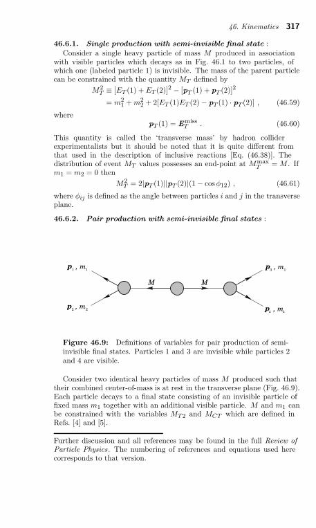
46. Kinematics 317
46.6.1. Single production with semi-invisible final state :
Consider a single heavy particle of mass M produced in associationwith visible particles which decays as in Fig. 46.1 to two particles, ofwhich one (labeled particle 1) is invisible. The mass of the parent particlecan be constrained with the quantity MT defined by
M2T ≡ [ET (1) + ET (2)]2 − [pT (1) + pT (2)]2
= m21 + m2
2 + 2[ET (1)ET (2) − pT (1) · pT (2)] , (46.59)
wherepT (1) = Emiss
T . (46.60)
This quantity is called the ‘transverse mass’ by hadron colliderexperimentalists but it should be noted that it is quite different fromthat used in the description of inclusive reactions [Eq. (46.38)]. Thedistribution of event MT values possesses an end-point at Mmax
T = M . Ifm1 = m2 = 0 then
M2T = 2|pT (1)||pT (2)|(1 − cosφ12) , (46.61)
where φij is defined as the angle between particles i and j in the transverseplane.
46.6.2. Pair production with semi-invisible final states :
p11
, mp44
, mp
, mp
3 1
22
, m
M M
Figure 46.9: Definitions of variables for pair production of semi-invisible final states. Particles 1 and 3 are invisible while particles 2and 4 are visible.
Consider two identical heavy particles of mass M produced such thattheir combined center-of-mass is at rest in the transverse plane (Fig. 46.9).Each particle decays to a final state consisting of an invisible particle offixed mass m1 together with an additional visible particle. M and m1 canbe constrained with the variables MT2 and MCT which are defined inRefs. [4] and [5].
Further discussion and all references may be found in the full Review of
Particle Physics. The numbering of references and equations used herecorresponds to that version.
318 48. Cross-section formulae for specific processes
48. CROSS-SECTION FORMULAE
FOR SPECIFIC PROCESSES
Revised October 2009 by H. Baer (University of Oklahoma) and R.N.Cahn (LBNL).
PART I: STANDARD MODEL PROCESSES
Setting aside leptoproduction (for which, see Sec. 16 of this Review),the cross sections of primary interest are those with light incident particles,e+e−, γγ, qq, gq , gg, etc., where g and q represent gluons and lightquarks. The produced particles include both light particles and heavyones - t, W , Z, and the Higgs boson H . We provide the production crosssections calculated within the Standard Model for several such processes.
48.1. Resonance Formation
Resonant cross sections are generally described by the Breit-Wignerformula (Sec. 19 of this Review).
σ(E) =2J + 1
(2S1 + 1)(2S2 + 1)
4π
k2
[
Γ2/4
(E − E0)2 + Γ2/4
]
BinBout, (48.1)
where E is the c.m. energy, J is the spin of the resonance, and thenumber of polarization states of the two incident particles are 2S1 + 1and 2S2 + 1. The c.m. momentum in the initial state is k, E0 is thec.m. energy at the resonance, and Γ is the full width at half maximumheight of the resonance. The branching fraction for the resonance intothe initial-state channel is Bin and into the final-state channel is Bout.For a narrow resonance, the factor in square brackets may be replaced byπΓδ(E − E0)/2.
48.2. Production of light particles
The production of point-like, spin-1/2 fermions in e+e− annihilationthrough a virtual photon, e+e− → γ∗ → ff , at c.m. energy squared s is
dσ
dΩ= Nc
α2
4sβ[1 + cos2 θ + (1 − β2) sin2 θ]Q2
f , (48.2)
where β is v/c for the produced fermions in the c.m., θ is the c.m.scattering angle, and Qf is the charge of the fermion. The factor Nc is 1for charged leptons and 3 for quarks. In the ultrarelativistic limit, β → 1,
σ = NcQ2f4πα2
3s= NcQ
2f
86.8 nb
s (GeV2). (48.3)
The cross section for the annihilation of a qq pair into a distinct pairq′q′ through a gluon is completely analogous up to color factors, with thereplacement α → αs. Treating all quarks as massless, averaging over thecolors of the initial quarks and defining t = −s sin2(θ/2), u = −s cos2(θ/2),one finds
dσ
dΩ(qq → q′q′) =
α2s
9s
t2 + u2
s2. (48.4)
Crossing symmetry gives
dσ
dΩ(qq′ → qq′) =
α2s
9s
s2 + u2
t2. (48.5)
If the quarks q and q′ are identical, we have
dσ
dΩ(qq → qq) =
α2s
9s
[
t2 + u2
s2+
s2 + u2
t2− 2u2
3st
]
, (48.6)
48. Cross-section formulae for specific processes 319
and by crossing
dσ
dΩ(qq → qq) =
α2s
9s
[
t2 + s2
u2+
s2 + u2
t2− 2s2
3ut
]
. (48.7)
Annihilation of e+e− into γγ has the cross section
dσ
dΩ(e+e− → γγ) =
α2
2s
u2 + t2
tu. (48.8)
The related QCD process also has a triple-gluon coupling. The crosssection is
dσ
dΩ(qq → gg) =
8α2s
27s(t2 + u2)(
1
tu− 9
4s2) . (48.9)
The crossed reactions are
dσ
dΩ(qg → qg) =
α2s
9s(s2 + u2)(− 1
su+
9
4t2) , (48.10)
dσ
dΩ(gg → qq) =
α2s
24s(t2 + u2)(
1
tu− 9
4s2) , (48.11)
dσ
dΩ(gg → gg) =
9α2s
8s(3 − ut
s2− su
t2− st
u2) . (48.12)
Lepton-quark scattering is analogous (neglecting Z exchange)
dσ
dΩ(eq → eq) =
α2
2se2qs2 + u2
t2, (48.13)
eq is the quark charge. For ν-scattering with the four-Fermi interaction
dσ
dΩ(νd → ℓ−u) =
G2F s
4π2, (48.14)
where the Cabibbo angle suppression is ignored. Similarly
dσ
dΩ(νu → ℓ−d) =
G2F s
4π2
(1 + cos θ)2
4. (48.15)
For deep inelastic scattering (presented in more detail in Section 19)we consider quarks of type i carrying a fraction x = Q2/(2Mν) of thenucleon’s energy, where ν = E − E′ is the energy lost by the lepton in thenucleon rest frame. With y = ν/E we have the correspondences
1 + cos θ → 2(1 − y) , dΩcm → 4πfi(x)dx dy , (48.16)where the latter incorporates the quark distribution, fi(x). We find
dσ
dx dy(eN → eX) =
4πα2xs
Q4
1
2
[
1 + (1 − y)2]
×[4
9(u(x) + u(x) + . . .)+
1
9(d(x) + d(x) + . . .)
]
(48.17)
where now s = 2ME is the cm energy squared for the electron-nucleoncollision and we have suppressed contributions from higher mass quarks.
Similarly,
dσ
dx dy(νN → ℓ−X) =
G2F xs
π[(d(x) + . . .) + (1 − y)2(u(x) + . . .)] , (48.18)
dσ
dx dy(νN → ℓ+X) =
G2F xs
π[(d(x) + . . .) + (1 − y)2(u(x) + . . .)] . (48.19)
Quasi-elastic neutrino scattering (νµn → µ−p, νµp → µ+n) is directlyrelated to the crossed reaction, neutron decay.
320 48. Cross-section formulae for specific processes
48.3. Hadroproduction of heavy quarks
For hadroproduction of heavy quarks Q = c, b, t, it is important toinclude mass effects in the formulae. For qq → QQ, one has
dσ
dΩ(qq → QQ) =
α2s
9s3
√
1 −4m2
Q
s
[
(m2Q − t)2 + (m2
Q − u)2 + 2m2Qs
]
,
(48.20)while for gg → QQ one has
dσ
dΩ(gg → QQ) =
α2s
32s
√
1 −4m2
Q
s
[
6
s2(m2
Q − t)(m2Q − u)
−m2
Q(s − 4m2Q)
3(m2Q − t)(m2
Q − u)+
4
3
(m2Q − t)(m2
Q − u) − 2m2Q(m2
Q + t)
(m2Q − t)2
+4
3
(m2Q − t)(m2
Q − u) − 2m2Q(m2
Q + u)
(m2Q − u)2
−3(m2
Q − t)(m2Q − u) + m2
Q(u − t)
s(m2Q − t)
−3(m2
Q − t)(m2Q − u) + m2
Q(t − u)
s(m2Q − u)
]
.
(48.21)
48.4. Production of Weak Gauge Bosons
48.4.1. W and Z resonant production :
Resonant production of a single W or Z is governed by the partial widths
Γ(W → ℓiνi) =
√2GF m3
W
12π(48.22)
Γ(W → qiqj) = 3
√2GF |Vij |2m3
W
12π(48.23)
Γ(Z → ff) = Nc
√2GF m3
Z
6π
×[
(T3 − Qf sin2 θW )2 + (Qf sin2 θW )2]
. (48.24)
The weak mixing angle is θW . The CKM matrix elements are Vij . Nc is 3for qq and 1 for leptonic final states. These widths along with associatedbranching fractions may be applied to the resonance production formulaof Sec. 48.1 to gain the total W or Z production cross section.
48.4.2. Production of pairs of weak gauge bosons :
The cross section for ff → W+W− is given in term of the couplings of theleft-handed and right-handed fermion f , ℓ = 2(T3 − QxW ), r = −2QxW ,where T3 is the third component of weak isospin for the left-handed f , Qis its electric charge (in units of the proton charge), and xW = sin2 θW :
dσ
dt=
2πα2
Ncs2
(
Q +ℓ + r
4xW
s
s − m2Z
)2
+
(
ℓ − r
4xW
s
s − m2Z
)2
A(s, t, u)
+1
2xW
(
Q +ℓ
2xW
s
s − m2Z
)
(Θ(−Q)I(s, t, u)− Θ(Q)I(s, u, t))
+1
8x2W
(Θ(−Q)E(s, t, u) + Θ(Q)E(s, u, t))
, (48.26)
48. Cross-section formulae for specific processes 321
where Θ(x) is 1 for x > 0 and 0 for x < 0, and where
A(s, t, u) =
(
tu
m4W
− 1
)(
1
4− m2
W
s+ 3
m4W
s2
)
+s
m2W
− 4,
I(s, t, u) =
(
tu
m4W
− 1
)(
1
4− m2
W
2s− m4
W
st
)
+s
m2W
− 2 + 2m2
W
t,
E(s, t, u) =
(
tu
m4W
− 1
)(
1
4+
m4W
t2
)
+s
m2W
, (48.27)
and s, t, u are the usual Mandelstam variables with s = (pf + pf )2, t =
(pf − pW−)2, u = (pf − pW+)2. The factor Nc is 3 for quarks and 1 forleptons.
The analogous cross-section for qiqj → W±Z0 is
dσ
dt=
πα2|Vij |26s2x2
W
(
1
s − m2W
)2 [(
9 − 8xW
4
)
(
ut − m2W m2
Z
)
+ (8xW − 6) s(
m2W + m2
Z
)]
+
[
ut − m2W m2
Z − s(m2W + m2
Z)
s − m2W
]
[
ℓj
t− ℓi
u
]
+ut − m2
W m2Z
4(1 − xW )
[
ℓ2jt2
+ℓ2iu2
]
+s(m2
W + m2Z)
2(1 − xW )
ℓiℓj
tu
, (48.28)
where ℓi and ℓj are the couplings of the left-handed qi and qj as definedabove. The CKM matrix element between qi and qj is Vij .
The cross section for qiqi → Z0Z0 is
dσ
dt=
πα2
96
ℓ4i + r4i
x2W (1 − x2
W )2s2
[
t
u+
u
t+
4m2Zs
tu− m4
Z
(
1
t2+
1
u2
)
]
.
(48.29)
48.5. Production of Higgs Bosons
48.5.1. Resonant Production :
The Higgs boson of the Standard Model can be produced resonantlyin the collisions of quarks, leptons, W or Z bosons, gluons, or photons.The production cross section is thus controlled by the partial width of theHiggs boson into the entrance channel and its total width. The partialwidths are given by the relations
Γ(H → ff) =GF m2
fmHNc
4π√
2
(
1 − 4m2f/m2
H
)3/2
, (48.30)
Γ(H → W+W−) =GF m3
HβW
32π√
2
(
4 − 4aW + 3a2W
)
, (48.31)
Γ(H → ZZ) =GF m3
HβZ
64π√
2
(
4 − 4aZ + 3a2Z
)
. (48.32)
where Nc is 3 for quarks and 1 for leptons and where aW = 1 − β2W =
4m2W /m2
H and aZ = 1 − β2Z = 4m2
Z/m2H . The decay to two gluons
proceeds through quark loops, with the t quark dominating. Explicitly,
322 48. Cross-section formulae for specific processes
Γ(H → gg) =α2
sGF m3H
36π3√
2
∣
∣
∣
∣
∣
∑
q
I(m2q/m2
H)
∣
∣
∣
∣
∣
2
, (48.33)
where I(z) is complex for z < 1/4. For z < 2 × 10⁻³, |I(z)| is small so thelight quarks contribute negligibly. For mH < 2mt, z > 1/4 and
I(z) = 3
[
2z + 2z(1 − 4z)
(
sin−1 1
2√
z
)2]
, (48.34)
which has the limit I(z) → 1 as z → ∞.
48.5.2. Higgs Boson Production in W∗ and Z
∗ decay :
The Standard Model Higgs boson can be produced in the decay ofa virtual W or Z (“Higgstrahlung”): In particular, if k is the c.m.momentum of the Higgs boson,
σ(qiqj → WH) =πα2|Vij |236 sin4 θW
2k√s
k2 + 3m2W
(s − m2W )2
(48.35)
σ(ff → ZH) =2πα2(ℓ2f + r2
f )
48Nc sin4 θW cos4 θW
2k√s
k2 + 3m2Z
(s − m2Z)2
. (48.36)
where ℓ and r are defined as above.
48.5.3. W and Z Fusion :Just as high-energy electrons can be regarded as sources of virtual photonbeams, at very high energies they are sources of virtual W and Z beams.For Higgs boson production, it is the longitudinal components of the W sand Zs that are important. The distribution of longitudinal W s carryinga fraction y of the electron’s energy is
f(y) =g2
16π2
1 − y
y, (48.37)
where g = e/ sin θW . In the limit s ≫ mH ≫ mW , the rate Γ(H →WLWL) = (g2/64π)(m3
H/m2W ) and in the equivalent W approximation
σ(e+e− → νeνeH) =1
16m2W
(
α
sin2 θW
)3
×[(
1 +m2
H
s
)
logs
m2H
− 2 + 2m2
H
s
]
. (48.38)
There are significant corrections to this relation when mH is not largecompared to mW . For mH = 150 GeV, the estimate is too high by 51%for
√s = 1000 GeV, 32% too high at
√s = 2000 GeV, and 22% too high
at√
s = 4000 GeV. Fusion of ZZ to make a Higgs boson can be treatedsimilarly. Identical formulae apply for Higgs production in the collisionsof quarks whose charges permit the emission of a W+ and a W−, exceptthat QCD corrections and CKM matrix elements are required. Even inthe absence of QCD corrections, the fine-structure constant ought to beevaluated at the scale of the collision, say mW . All quarks contribute tothe ZZ fusion process.
Further discussion and all references may be found in the full Review; theequation and reference numbering corresponds to that version.
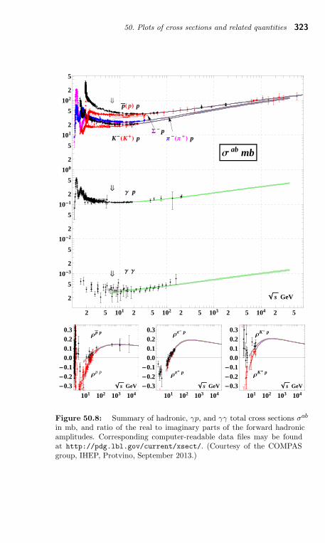
50. Plots of cross sections and related quantities 323
2 5 101 2 5 102 2 5 103 2 5 104 2 5
2
5
10-3
2
5
10-2
2
5
10-1
2
5
100
2
5
101
2
5
102
2
5
s GeV
pHpL p
K-HK+L p Π -HΠ +L pS - p
Γ p
Γ Γ
Σ ab mb
ß
ß
ß
101 102 103 104
-0.3-0.2-0.1
0.00.10.20.3
Ρp p
Ρp p
s GeV
101 102 103 104
-0.3-0.2-0.1
0.00.10.20.3
ΡΠ- p
ΡΠ+ p
s GeV
101 102 103 104
-0.3-0.2-0.1
0.00.10.20.3
ΡK- p
ΡK+ p
s GeV
Figure 50.8: Summary of hadronic, γp, and γγ total cross sections σab
in mb, and ratio of the real to imaginary parts of the forward hadronicamplitudes. Corresponding computer-readable data files may be foundat http://pdg.lbl.gov/current/xsect/. (Courtesy of the COMPASgroup, IHEP, Protvino, September 2013.)
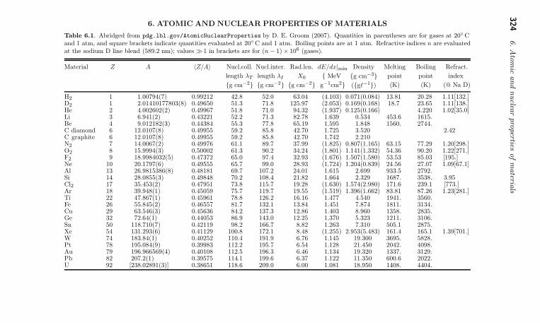
324
6.A
tom
icand
nuclea
rpro
pertiesofm
ateria
ls6. ATOMIC AND NUCLEAR PROPERTIES OF MATERIALS
Table 6.1. Abridged from pdg.lbl.gov/AtomicNuclearProperties by D. E. Groom (2007). Quantities in parentheses are for gases at 20 Cand 1 atm, and square brackets indicate quantities evaluated at 20 C and 1 atm. Boiling points are at 1 atm. Refractive indices n are evaluatedat the sodium D line blend (589.2 nm); values ≫ 1 in brackets are for (n − 1) × 106 (gases).
Material Z A 〈Z/A〉 Nucl.coll.
length λT
g cm−2
Nucl.inter.
length λI
g cm−2
Rad.len.
X0
g cm−2
dE/dx|min
MeV
g−1cm2
Density
g cm−3
(gℓ−1)
Melting
point
(K)
Boiling
point
(K)
Refract.
index
(@ Na D)
H2 1 1.00794(7) 0.99212 42.8 52.0 63.04 (4.103) 0.071(0.084) 13.81 20.28 1.11[132.]D2 1 2.01410177803(8) 0.49650 51.3 71.8 125.97 (2.053) 0.169(0.168) 18.7 23.65 1.11[138.]He 2 4.002602(2) 0.49967 51.8 71.0 94.32 (1.937) 0.125(0.166) 4.220 1.02[35.0]Li 3 6.941(2) 0.43221 52.2 71.3 82.78 1.639 0.534 453.6 1615.Be 4 9.012182(3) 0.44384 55.3 77.8 65.19 1.595 1.848 1560. 2744.C diamond 6 12.0107(8) 0.49955 59.2 85.8 42.70 1.725 3.520 2.42C graphite 6 12.0107(8) 0.49955 59.2 85.8 42.70 1.742 2.210N2 7 14.0067(2) 0.49976 61.1 89.7 37.99 (1.825) 0.807(1.165) 63.15 77.29 1.20[298.]O2 8 15.9994(3) 0.50002 61.3 90.2 34.24 (1.801) 1.141(1.332) 54.36 90.20 1.22[271.]F2 9 18.9984032(5) 0.47372 65.0 97.4 32.93 (1.676) 1.507(1.580) 53.53 85.03 [195.]Ne 10 20.1797(6) 0.49555 65.7 99.0 28.93 (1.724) 1.204(0.839) 24.56 27.07 1.09[67.1]Al 13 26.9815386(8) 0.48181 69.7 107.2 24.01 1.615 2.699 933.5 2792.Si 14 28.0855(3) 0.49848 70.2 108.4 21.82 1.664 2.329 1687. 3538. 3.95Cl2 17 35.453(2) 0.47951 73.8 115.7 19.28 (1.630) 1.574(2.980) 171.6 239.1 [773.]Ar 18 39.948(1) 0.45059 75.7 119.7 19.55 (1.519) 1.396(1.662) 83.81 87.26 1.23[281.]Ti 22 47.867(1) 0.45961 78.8 126.2 16.16 1.477 4.540 1941. 3560.Fe 26 55.845(2) 0.46557 81.7 132.1 13.84 1.451 7.874 1811. 3134.Cu 29 63.546(3) 0.45636 84.2 137.3 12.86 1.403 8.960 1358. 2835.Ge 32 72.64(1) 0.44053 86.9 143.0 12.25 1.370 5.323 1211. 3106.Sn 50 118.710(7) 0.42119 98.2 166.7 8.82 1.263 7.310 505.1 2875.Xe 54 131.293(6) 0.41129 100.8 172.1 8.48 (1.255) 2.953(5.483) 161.4 165.1 1.39[701.]W 74 183.84(1) 0.40252 110.4 191.9 6.76 1.145 19.300 3695. 5828.Pt 78 195.084(9) 0.39983 112.2 195.7 6.54 1.128 21.450 2042. 4098.Au 79 196.966569(4) 0.40108 112.5 196.3 6.46 1.134 19.320 1337. 3129.Pb 82 207.2(1) 0.39575 114.1 199.6 6.37 1.122 11.350 600.6 2022.U 92 [238.02891(3)] 0.38651 118.6 209.0 6.00 1.081 18.950 1408. 4404.
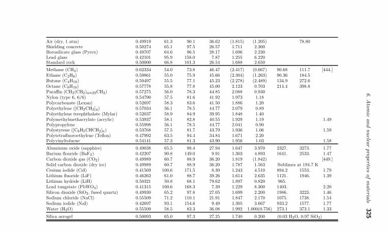
6.A
tom
icand
nuclea
rpro
pertiesofm
ateria
ls325
Air (dry, 1 atm) 0.49919 61.3 90.1 36.62 (1.815) (1.205) 78.80Shielding concrete 0.50274 65.1 97.5 26.57 1.711 2.300Borosilicate glass (Pyrex) 0.49707 64.6 96.5 28.17 1.696 2.230Lead glass 0.42101 95.9 158.0 7.87 1.255 6.220Standard rock 0.50000 66.8 101.3 26.54 1.688 2.650
Methane (CH4) 0.62334 54.0 73.8 46.47 (2.417) (0.667) 90.68 111.7 [444.]Ethane (C2H6) 0.59861 55.0 75.9 45.66 (2.304) (1.263) 90.36 184.5Butane (C4H10) 0.59497 55.5 77.1 45.23 (2.278) (2.489) 134.9 272.6Octane (C8H18) 0.57778 55.8 77.8 45.00 2.123 0.703 214.4 398.8Paraffin (CH3(CH2)n≈23CH3) 0.57275 56.0 78.3 44.85 2.088 0.930Nylon (type 6, 6/6) 0.54790 57.5 81.6 41.92 1.973 1.18Polycarbonate (Lexan) 0.52697 58.3 83.6 41.50 1.886 1.20Polyethylene ([CH2CH2]n) 0.57034 56.1 78.5 44.77 2.079 0.89Polyethylene terephthalate (Mylar) 0.52037 58.9 84.9 39.95 1.848 1.40Polymethylmethacrylate (acrylic) 0.53937 58.1 82.8 40.55 1.929 1.19 1.49Polypropylene 0.55998 56.1 78.5 44.77 2.041 0.90Polystyrene ([C6H5CHCH2]n) 0.53768 57.5 81.7 43.79 1.936 1.06 1.59Polytetrafluoroethylene (Teflon) 0.47992 63.5 94.4 34.84 1.671 2.20Polyvinyltoluene 0.54141 57.3 81.3 43.90 1.956 1.03 1.58
Aluminum oxide (sapphire) 0.49038 65.5 98.4 27.94 1.647 3.970 2327. 3273. 1.77Barium flouride (BaF2) 0.42207 90.8 149.0 9.91 1.303 4.893 1641. 2533. 1.47Carbon dioxide gas (CO2) 0.49989 60.7 88.9 36.20 1.819 (1.842) [449.]Solid carbon dioxide (dry ice) 0.49989 60.7 88.9 36.20 1.787 1.563 Sublimes at 194.7 KCesium iodide (CsI) 0.41569 100.6 171.5 8.39 1.243 4.510 894.2 1553. 1.79Lithium fluoride (LiF) 0.46262 61.0 88.7 39.26 1.614 2.635 1121. 1946. 1.39Lithium hydride (LiH) 0.50321 50.8 68.1 79.62 1.897 0.820 965.Lead tungstate (PbWO4) 0.41315 100.6 168.3 7.39 1.229 8.300 1403. 2.20Silicon dioxide (SiO2, fused quartz) 0.49930 65.2 97.8 27.05 1.699 2.200 1986. 3223. 1.46Sodium chloride (NaCl) 0.55509 71.2 110.1 21.91 1.847 2.170 1075. 1738. 1.54Sodium iodide (NaI) 0.42697 93.1 154.6 9.49 1.305 3.667 933.2 1577. 1.77Water (H2O) 0.55509 58.5 83.3 36.08 1.992 1.000(0.756) 273.1 373.1 1.33
Silica aerogel 0.50093 65.0 97.3 27.25 1.740 0.200 (0.03 H2O, 0.97 SiO2)

326 NOTES

NOTES 327

328 NOTES
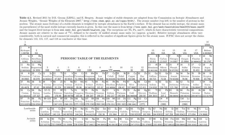
Table 4.1. Revised 2011 by D.E. Groom (LBNL), and E. Bergren. Atomic weights of stable elements are adapted from the Commission on Isotopic Abundances andAtomic Weights, “Atomic Weights of the Elements 2007,” http://www.chem.qmul.ac.uk/iupac/AtWt/. The atomic number (top left) is the number of protons in thenucleus. The atomic mass (bottom) of a stable elements is weighted by isotopic abundances in the Earth’s surface. If the element has no stable isotope, the atomic mass(in parentheses) of the most stable isotope currently known is given. In this case the mass is from http://www.nndc.bnl.gov/amdc/masstables/Ame2003/mass.mas03
and the longest-lived isotope is from www.nndc.bnl.gov/ensdf/za form.jsp. The exceptions are Th, Pa, and U, which do have characteristic terrestrial compositions.Atomic masses are relative to the mass of 12C, defined to be exactly 12 unified atomic mass units (u) (approx. g/mole). Relative isotopic abundances often varyconsiderably, both in natural and commercial samples; this is reflected in the number of significant figures given for the atomic mass. IUPAC does not accept the claimsfor elements 113, 115, 117, and 118 as conclusive at this time.
1IA
18VIIIA
1 HHydrogen
1.007942
IIA13IIIA
14IVA
15VA
16VIA
17VIIA
2 HeHelium
4.0026023 LiLithium
6.941
4 BeBeryllium
9.012182
PERIODIC TABLE OF THE ELEMENTS
5 BBoron
10.811
6 CCarbon
12.0107
7 NNitrogen
14.0067
8 OOxygen
15.9994
9 FFluorine
18.9984032
10 NeNeon
20.1797
11 NaSodium
22.98976928
12 MgMagnesium
24.30503
IIIB4
IVB5
VB6
VIB7
VIIB8 9
VIII10 11
IB12IIB
13 AlAluminum
26.9815386
14 SiSilicon
28.0855
15 PPhosph.
30.973762
16 SSulfur
32.065
17 ClChlorine
35.453
18 ArArgon
39.948
19 KPotassium
39.0983
20 CaCalcium
40.078
21 ScScandium
44.955912
22 TiTitanium
47.867
23 VVanadium
50.9415
24 CrChromium
51.9961
25 MnManganese
54.938045
26 FeIron
55.845
27 CoCobalt
58.933195
28 NiNickel
58.6934
29 CuCopper
63.546
30 ZnZinc
65.38
31 GaGallium
69.723
32 GeGerman.
72.64
33 AsArsenic
74.92160
34 SeSelenium
78.96
35 BrBromine
79.904
36 KrKrypton
83.79837 RbRubidium
85.4678
38 SrStrontium
87.62
39 YYttrium
88.90585
40 ZrZirconium
91.224
41 NbNiobium
92.90638
42 MoMolybd.
95.96
43 TcTechnet.
(97.90722)
44 RuRuthen.
101.07
45 RhRhodium
102.90550
46 PdPalladium
106.42
47 AgSilver
107.8682
48 CdCadmium
112.411
49 InIndium
114.818
50 SnTin
118.710
51 SbAntimony
121.760
52 TeTellurium
127.60
53 IIodine
126.90447
54 XeXenon
131.29355 CsCesium
132.9054519
56 BaBarium
137.327
57–71Lantha-
nides
72 HfHafnium
178.49
73 TaTantalum
180.94788
74 WTungsten
183.84
75 ReRhenium
186.207
76 OsOsmium
190.23
77 IrIridium
192.217
78 PtPlatinum
195.084
79 AuGold
196.966569
80 HgMercury
200.59
81 TlThallium
204.3833
82 PbLead
207.2
83 BiBismuth
208.98040
84 PoPolonium
(208.98243)
85 AtAstatine
(209.98715)
86 RnRadon
(222.01758)
87 FrFrancium
(223.01974)
88 RaRadium
(226.02541)
89–103Actinides
104 RfRutherford.
(267.122)
105 DbDubnium
(268.125)
106 SgSeaborg.
(271.133)
107 BhBohrium
(270.134)
108 HsHassium
(269.134)
109 MtMeitner.
(276.151)
110 DsDarmstadt.
(281.162)
111 RgRoentgen.
(280.164)
112 CnCopernicium
(277)
114 FlFlerovium
(289)
116 LvLivermorium
(288)
Lanthanideseries
57 LaLanthan.
138.90547
58 CeCerium
140.116
59 PrPraseodym.
140.90765
60 NdNeodym.
144.242
61 PmPrometh.
(144.91275)
62 SmSamarium
150.36
63 EuEuropium
151.964
64 GdGadolin.
157.25
65 TbTerbium
158.92535
66 DyDyspros.
162.500
67 HoHolmium
164.93032
68 ErErbium
167.259
69 TmThulium
168.93421
70 YbYtterbium
173.054
71 LuLutetium
174.9668
Actinideseries
89 AcActinium
(227.02775)
90 ThThorium
232.03806
91 PaProtactin.
231.03588
92 UUranium
238.02891
93 NpNeptunium
(237.04817)
94 PuPlutonium
(244.06420)
95 AmAmeric.
(243.06138)
96 CmCurium
(247.07035)
97 BkBerkelium
(247.07031)
98 CfCaliforn.
(251.07959)
99 EsEinstein.
(252.0830)
100 FmFermium
(257.09510)
101 MdMendelev.
(258.09843)
102 NoNobelium
(259.1010)
103 LrLawrenc.
(262.110)

2014
JULY AUGUST SEPTEMBER
S M T W T F S S M T W T F S S M T W T F S
1 2 3 4 5
6 7 8 9 10 11 12
13 14 15 16 17 18 19
20 21 22 23 24 25 26
27 28 29 30 31
1 2
3 4 5 6 7 8 9
10 11 12 13 14 15 16
17 18 19 20 21 22 23
24 25 26 27 28 29 30
31
1 2 3 4 5 6
7 8 9 10 11 12 13
14 15 16 17 18 19 20
21 22 23 24 25 26 27
28 29 30
OCTOBER NOVEMBER DECEMBER
S M T W T F S S M T W T F S S M T W T F S
1 2 3 4
5 6 7 8 9 10 11
12 13 14 15 16 17 18
19 20 21 22 23 24 25
26 27 28 29 30 31
1
2 3 4 5 6 7 8
9 10 11 12 13 14 15
16 17 18 19 20 21 22
23 24 25 26 27 28 29
30
1 2 3 4 5 6
7 8 9 10 11 12 13
14 15 16 17 18 19 20
21 22 23 24 25 26 27
28 29 30 31
2015
JULY AUGUST SEPTEMBER
S M T W T F S S M T W T F S S M T W T F S
1 2 3 4
5 6 7 8 9 10 11
12 13 14 15 16 17 18
19 20 21 22 23 24 25
26 27 28 29 30 31
1
2 3 4 5 6 7 8
9 10 11 12 13 14 15
16 17 18 19 20 21 22
23 24 25 26 27 28 29
30 31
1 2 3 4 5
6 7 8 9 10 11 12
13 14 15 16 17 18 19
20 21 22 23 24 25 26
27 28 29 30
OCTOBER NOVEMBER DECEMBER
S M T W T F S S M T W T F S S M T W T F S
1 2 3
4 5 6 7 8 9 10
11 12 13 14 15 16 17
18 19 20 21 22 23 24
25 26 27 28 29 30 31
1 2 3 4 5 6 7
8 9 10 11 12 13 14
15 16 17 18 19 20 21
22 23 24 25 26 27 28
29 30
1 2 3 4 5
6 7 8 9 10 11 12
13 14 15 16 17 18 19
20 21 22 23 24 25 26
27 28 29 30 31
2015
JANUARY FEBRUARY MARCH
S M T W T F S S M T W T F S S M T W T F S
1 2 3
4 5 6 7 8 9 10
11 12 13 14 15 16 17
18 19 20 21 22 23 24
25 26 27 28 29 30 31
1 2 3 4 5 6 7
8 9 10 11 12 13 14
15 16 17 18 19 20 21
22 23 24 25 26 27 28
1 2 3 4 5 6 7
8 9 10 11 12 13 14
15 16 17 18 19 20 21
22 23 24 25 26 27 28
29 30 31
APRIL MAY JUNE
S M T W T F S S M T W T F S S M T W T F S
1 2 3 4
5 6 7 8 9 10 11
12 13 14 15 16 17 18
19 20 21 22 23 24 25
26 27 28 29 30
1 2
3 4 5 6 7 8 9
10 11 12 13 14 15 16
17 18 19 20 21 22 23
24 25 26 27 28 29 30
31
1 2 3 4 5 6
7 8 9 10 11 12 13
14 15 16 17 18 19 20
21 22 23 24 25 26 27
28 29 30
2016
JANUARY FEBRUARY MARCH
S M T W T F S S M T W T F S S M T W T F S
1 2
3 4 5 6 7 8 9
10 11 12 13 14 15 16
17 18 19 20 21 22 23
24 25 26 27 28 29 30
31
1 2 3 4 5 6
7 8 9 10 11 12 13
14 15 16 17 18 19 20
21 22 23 24 25 26 27
28 29
1 2 3 4 5
6 7 8 9 10 11 12
13 14 15 16 17 18 19
20 21 22 23 24 25 26
27 28 29 30 31
APRIL MAY JUNE
S M T W T F S S M T W T F S S M T W T F S
1 2
3 4 5 6 7 8 9
10 11 12 13 14 15 16
17 18 19 20 21 22 23
24 25 26 27 28 29 30
1 2 3 4 5 6 7
8 9 10 11 12 13 14
15 16 17 18 19 20 21
22 23 24 25 26 27 28
29 30 31
1 2 3 4
5 6 7 8 9 10 11
12 13 14 15 16 17 18
19 20 21 22 23 24 25
26 27 28 29 30
Prep
ared
for
the
U.S
.D
epartm
ent
ofE
nerg
yunder
Contra
ctD
E-A
C02-0
5C
H11231


