
Federal Reserve Bank of MinneapolisResearch Department Staff Report ???
April 9, 2007
Restructuring the Sovereign Debt Restructuring Mechanism
Rohan Pitchford∗
University of Sydney
Mark L. J. Wright∗
University of California, Los Angeles
ABSTRACT
Sovereign defaults are time consuming and costly to resolve. But these costs also improve borrowingincentives ex ante. What is the optimal tradeoff between efficient borrowing ex ante and the costs ofdefault ex post? What policy reforms, from collective action clauses to an international bankruptcycourt, would attain this optimal tradeoff? Towards an answer to these questions, this paper presentsan incomplete markets model of sovereign borrowing default coupled with an explicit model of thesovereign debt restructuring process in which delay arises due to both creditor holdout and free-riding on negotiation effort. We characterize the ex ante optimal amount of delay, and explorenumerically the effects of various policy options on the amount of delay in renegotiations, and onthe efficiency of capital flows.
∗Very preliminary and incomplete. We thank ... for helpful comments. Further comments welcome.

1. Introduction
Sovereign defaults are time consuming and costly to resolve. For example, the 1980’s
debt crisis took more than one decade and two US Treasury Plans before culminating in
settlements under the Brady Plan. The recent default by Argentina took four years from
initial default to exchange offer, and still lingers as creditors explore legal options. A number
of studies (for example, Suter 1993) have shown that this pattern was also common in history,
with the median time to settle defaults in excess of ten years. This delay is also costly.
As shown in Figure One, sovereign capital flows to Argentina dropped to approximately
zero during its most recent default, while Miller, Tomz and Wright (2005) document similar
declines for a wide range of countries over a long period of history. That is, the sovereign
governments of countries in default appear to be cut off from access to international capital
markets.
As a result of these costs, it is hardly surprising that there has been a great deal of
discussion in policy circles of potential changes to the workings of sovereign debt markets
and restructuring negotiations with a view to reducing the costs of default. These poten-
tial changes to the so-called “sovereign debt restructuring mechanism” (SDRM) range from
policies that de-emphasize the involvement of supra-national institutions focusing on private
sector initiatives and changes to contract details including the addition of “collective action
clauses” (Eichengreen 2002, Taylor 2001), to the re-introduction of the bondholder represen-
tative groups that mediated debt settlements at the turn of the 20th Century (Eichengreen
and Portes 1995), all the way to the establishment of an international bankruptcy court
(Krueger 2001, 2002).
But this policy effort faces a fundamental dilemma. Although negotiation protocols
and contract structures that are complicated and time consuming to implement impose great
costs on a defaulting country ex post, these same costs also give a country an incentive to avoid
default, and to borrow efficiently ex ante. Indeed some authors, such as Dooley (2002), have
argued that the difficulties that exist with regard to restructuring sovereign debt contracts
are the deliberate response by both creditors and debtor countries to this incentive problem.
In the light of this debate, this paper asks: what features of the current sovereign debt

restructuring mechanism lead to slow and costly default resolution? what is the optimal
trade-off between efficient borrowing ex ante and the costs of default ex post? and what
policy reforms, by both international institutions and creditor country governments on one
side, as well as by debtor countries themselves, are available to attain this optimal trade-off?
Towards an answer to these questions, this paper begins by reviewing recent expe-
rience with sovereign debt restructuring. We characterize the amount of delay observed,
and review the debate on the causes of this delay. We then present an explicit model of
the sovereign debt restructuring process designed to capture the features emphasized in the
policy discussion. We make one key assumption — that creditors cannot commit to begin
negotiations at any specific time — and study the amount of delay produced under a number
of different assumptions on the bargaining process that are intended to capture features of
the process that are currently in place, as well as a number of the policy proposals that are
currently on the table. In negotiations, delay may arise because creditors hold out for better
settlements or because they free ride on the negotiation effort of others. We then calibrate
this model to match data on the restructuring process and find that the model does a good
job matching restructuring outcomes.
We then embed this bargaining model in a simple incomplete contracting model of
sovereign borrowing. Countries borrow to finance profitable investments, and cannot commit
to repay their debts, defaulting opportunistically whenever it is in their best interests. The
only loan instruments are state non-contingent bonds, and so default can be socially desirable
in some states of the world. We then use this model to characterize the optimal amount of
delay, and to understand the effect of various policy options.
This paper draws on a number of related literatures concerning both sovereign debt
and holdout in bargaining. The basic borrowing framework is an example of an incomplete
contracting model of debt. The first to apply this framework to a study of sovereign debt
were Eaton and Gersovitz (1983), whos work has since been extended by Arellano (2005),
Aguiar and Gopinath (2006), Irani (2006) and many others. Unlike all of these papers,
which assume that default is punished by an exogenous deterministic or stochastic process
of exclusion from financial markets, we model the punishments to default as arising from an
explicitly specified debt restructuring bargaining game. In a recent paper, Yue (2006) studies
2

the effect of bargaining on default settlement on implied bond yields in a model that produces
much less delay in bargaining, and hence also much shorter lengths of exclusion form financial
markets, than is found in the historical record. In contrast, our model aims to explain the
entire distribution of bargaining delays observed in the data, and then uses these results to
examine the normative implications of different policy regimes.
In the restructuring model of the paper, creditors must decide on when to enter into
negotiations and, once in negotiations, on their bargaining strategy. The decision to enter
into negotiations shares some features with simple timing games such as the war of attrition
studied by Hendricks, Weiss and Wilson (1988) and many others. Once negotiations have be-
gun, bargaining takes place using a modified version of the alternating offer model introduced
by Rubinstein (1982) and extended by Binmore (1987) and many others. Although the model
assumes complete information, delay is a feature of all equilibria and so the model provides
a counter-example to the commonly heard claim that imperfect information is necessary for
delay to occur in bargaining models (see also, Fernandez and Glazer 1991). It is also worth
noting that some bargaining games with incomplete information give rise to results which
also echo the war of attrition (for example, Osbourne 1985 and Abreu and Gul 2000).
Finally, this paper is related to efforts aimed at understanding the welfare effects
of changes in domestic bankruptcy systems such as Livshits, MacGee and Tertilt (2003).
However, in contrast to their model which takes the bankruptcy system as a fixed set of
parameters which is varied as a result of legislative reform, our model derives the form of
debt restructuring as the equilibrium of a game that is then matched to observed restructuring
outcomes. Policy is then examined in terms of modifications on the parameters and structure
of this game.
The rest of this paper is structured as follows. Section 2 describes our data on de-
faults and settlements and provides a survey of forces that would appear to be important
in determining delay in restructuring negotiations in practice. Section 3 introduces our ex-
plicit model of the settlement bargaining process and shows how different assumptions on
the number of creditors, the type of debt contracts, and different aspects of the bargaining
environment translate into different amounts of delay in negotiations. Section 4 then outlines
the borrowing environment and characterizes the results for welfare in terms of the features
3

of the renegotiation process, while Section 5 concludes.
2. Sovereign Debt Restructuring in Practice
In this section, we survey restructuring negotiations of the past two centuries with a
view to isolating factors that may contribute to delay.
A. Data on Sovereign Debt Restructuring
To begin, we examine data on the amount of time taken to conclude negotiations to
resolve sovereign defaults. We follow standard practice in defining a sovereign default to have
occurred if either a country fails to meet its contractual obligations, or if it restructures its
debts on unfavourable terms. The latter may involve instances in which creditors appear to
voluntarily exchange their bonds.
We obtain dates for the beginning of a default according to this definition from Stan-
dard and Poors (Beers and Chambers 2004), who in turn rely on the historical work of Suter
(1990, 1992). The data cover the entire period from the end of the Napoleonic wars to the
present. A default is defined to have ended when a supermajority of creditors agrees to a
restructuring. Once again we rely on Standard and Poors for providing end dates.
In some cases, the Standard and Poors dates may understate the length of a default. In
particular, to the extent that a default is defined as an unfavourable restructuring, Standard
and Poors dates the beginning of the default as the date of the restructuring which may
ignore preceeding negotiations. In addition, Standard and Poors reports only the year the
default began and ended, and consequently the length of short defaults is typically truncated
to zero. To rectify these problems, we examined a range of primary and secondary sources
to obtain the month, and in some cases the day, in which defaults began or negotiations
were terminated. Most notable amongst these sources were Duggan and Tomz (2006) for the
historical data, while for the modern period we relied on theWorld Banks’Global Development
Finance the Institute for International Finance’s Surveys of Debt Restructuring, and Cline
(1996).1
1An alternative, and in some cases more preferable and more model consistent, approach would define the
4

Delay
num. Mean Std. Dev. Skew
Whole sample 272 8.8 10.5 2.2
- ex. communist 267 8.1 9.1 1.9
Defaults Ended During
1824-1867 23 15.0 5.3 4.9
1868-1917 50 7.9 5.4 6.2
1918-1975 52 9.5 5.7 4.7
1976-2005 147 6.5 6.3 2.1
1981-2005 136 6.9 6.2 2.2
1991-2005 97 8.7 6.2 2.3
Some summary statistics on the lengths of defaults are presented in Table One. Ac-
cording to our measure, from 1824 to the present, there have been 272 defaults which on
average lasted for just under nine years. If we exclude the communist defaults of the early
Twentieth Century, which turned out to be especially long and arguably involve considera-
tions outside of our analysis below, the average length of a default drops to just over eight
years. There was also an extraordinary amount of variation in the length of time that it took
for sovereign debts to be restructured, with a standard deviation in excess of nine years.
Although there has been substantial variation in the lengths of defaults over time,
these patterns are not driven by the long time horizon. Grouping defaults by the time period
in which they ended (in an attempt to capture the different institutional arrangements that
governed restructuring in different time periods) we find that the defaults of the first half of
the 19th Century, before the formation of bondholder representative groups like the British
Corporation of Foreign Bondholders (CFB), lasted more than twice as long as defaults in the
modern period. Following the formation of the CFB in 1868 and upon to the First World
War, default lengths declined to about eight years on average. Defaults lengths then rose in
the interwar period, driven presumably by the long defaults following the Great Depression,
end of a default to have occurred when net borrowing by a sovereign becomes positive. Early efforts alongthese lines have been presented for the modern period in Miller, Tomz and Wright (2005) and Richmond(2007).
5

before falling to six and one-half years in the modern period, which we define as beginning
with the passage of the US Foreign Sovereign Immunities Act in 1976 which changed to legal
basis of sovereign debt restructuring. Default lengths have stayed roughly constant during
this period with the exception of a lengthening of defaults concluded in the 1990s which
reflects the resolution of the debt crisis of the 1980s.
Strikingly, the standard deviation for default lengths remained large, and in the mod-
ern period was approximately equal to the mean default duration: there is, quite simply, an
enormous amount of variation in the amount of time it takes to settle a default. The fact that
the standard deviation of default durations is also approximately equal to the mean default
duration also tells us something about the underlying process governing debt restructuring.
In particular, this fact suggests that the distribution of delay may be well approximated by
an exponential distribution, an observation which is further strengthened by noting that the
skewness of the empirical distribution is approximately equal to two (which is a characteristic
of the exponential). We will return to this observation below when we examine the empirical
implications of our bargaining model.
B. Explaining the Delay in Bargaining
Delay in bargaining has been the subject of a substantial theoretical literature, with
a great deal of effort devoted to the role of delay in signalling private information between
parties. Arguably, the abundance of information about national economies suggests that
private information is unlikely to be the main source of delay in bargaining over sovereign
debt restructuring. In what follows, we examine some case studies of delays in sovereign debt
restructuring for insights as to the causes of that delay which will then guide the development
of our model.
Holdout and “Vulture Creditors”
The restructuring case that has garnered the most attention, and which has formed
the basis for a number of the policy proposals aimed at restructuring the sovereign debt
restructuring mechanism, has been the restructuring of Peru’s debts in the mid 1990s under
6

the Brady Plan following its default in 1983. The reason for this attention has been the
actions of the “vulture creditors” Elliot Associates who at one point threatened to hold up
the entire restructuring effort.
A brief version of the story of this case begins in 1996 when Elliot Associates purchased,
on secondary markets, a number of deeply discounted securitized bank loans. Court records
show that Elliot Associates bought $11.4m of Peruvian debt with a face value of $20.7m,
not including deferred interest. In 1997 Peru closed its Brady Exchange deal which received
the support of more than 95% of its creditors. of the creditors who did not settle, Elliot
Associated was one of the largest. Elliot then proceeded through a number of various legal
avenues to force Peru to settle its outstanding debts at face value, plus deferred interest. In
1999, Elliot Associated obtained a judgment against Peru for the entire amount by which the
debt was in arrears.
This was not in itself unusual: since the passage of the Foreign Sovereign Immuni-
ties Act in 1976, private citizens have been able to bring suit against a foreign sovereign
government in the United States, while similar provisions were passed during the 1970s in
most other countries with an English legal tradition. However, legal actions against sovereign
countries have typically been fruitless in the sense that it has been extremely difficult to
attach assets following a judgment. Courts have typically held that the assets of state owned
corporations are immune from attachment, and sovereign countries rarely hold other assets
outside of their borders. Those assets that are held offshore, such as central bank reserves,
are typically immune from seizure by international treaty.
Elliot Associates adopted the novel strategy of pursuing the interest payments on
Peru’s new debts under the Brady Plan. Specifically, Elliot Associated sought the attach-
ment of the funds that were going to be used to pay coupons on the new Brady Bonds. In
2000, Elliot Associates obtained an injunction against Peru paying interest on the new debts.
Coming just before a coupon payment was due, this forced Peru into the position of either
having to settle with Elliot, or default on the interest payments on its new debts. As a result,
Peru elected to settle for $59m.
Although striking, the Elliot Associated case was not new. Other court cases had
been pursued against defaulting sovereign countries in the 1980s and 1990s, including most
7

notably the unsuccessful Allied Bank v. Costa Rica (1981) case, and the successful EM
Ltd. v. Brazil case of 1995 which involved the notorious creditor Kenneth Dart. There are
also earlier historical episodes with a similar flavor in which creditors attempted to use the
London Stock Exchange’s prohibition against the listing of new securities issued by a country
in default to force a settlement.2 However, Elliot Associates was in many was the inspiration
for new creditor efforts to extract funds and, indeed, Elliot Associates and EM Ltd. were at
the forefront of the more than 140 court cases that were brought against Argentina during
its new restructuring.3
The key feature of the Elliot case, as well as some other related cases, is that hold-out
creditors appear able to disrupt a countries efforts to service new debts. This is important
because, if creditors begin to anticipate such efforts, they will not be prepared to issue new
debts to a country until all of its remaining creditors have settled. Essentially, each creditor
has veto power over a countries ability to re-access international financial markets. It is this
de facto veto power that will be one feature of the model in the next section.
Free Riding on Negotiation Effort
Importantly, it is worth noting that despite the possible benefits to holding out in the
manner of Elliot Associates, it is common to see most creditors either settle on common terms
(sometimes from a menu of options) or join a common holdout strategy. This is despite the
fact that the veto power over market reaccess that underlies the success of vulture creditor
strategies of itself imparts a strong incentive for all creditors to negotiate individually: no
matter the amount that a country has settled for with other creditors, the last creditor
to settle retains the veto and can extract better terms. This suggests that there must be
substantial costs to negotiation that limit the incentives of small creditors to negotiate on
their own. Such costs, in turn, can lead to an additional incentive to delay in order to free
ride on the negotiation costs of others.
2Perhaps the best known concern the rival Spanish bondholder committees who’s disputes in the 1850sled indirectly to the formation of the Council (and later Corporation) of Foreign Bondholders in 1868.
3Although ongoing, these suits against Argentina have so far proven unsuccessful which in part may reflectthe efforts of the US government in arguing that such holdout is undesirable. It should be noted that, for ourpurposes, all that is required to produce delay is the expectation of a higher return from legal action. Ourmodel below will be used to question the wisdom of the US governments position.
8

What little direct evidence we have suggests that the negotiation costs are substantial.
The CFB, whos annual reports are public, typically charged bondholders a fee of one-half of
one per cent of the face value of new securities to defray negotiation costs. This fee likely
understates the size of these costs: in most years, half of the expenses of the CFB were directly
subsidized by the Bank of England, while expenses themselves tended to be understated due
to the fact that all office holders donated their time and the fact that the CFB often made
substantial use (without charge) of UK diplomatic and consular resources during negotiations
with foreign sovereigns.
In the modern period, bank action committees may have been able to partially resolve
this problem by requiring subscriptions from members and by negotiating for fees to be paid
directly by the defaulting country, although the extent of the latter was presumably limited to
costs that were verifiable. In the modern period, half a dozen or more bondholder presentative
bodies participated in discussions with the Argentine government, although most restricted
membership to institutional investors who agreed to bear the negotiation costs.4
In the next section, we posit the existence of fixed costs of negotiation both as a
source of delay (due to free riding) and as a tool for generating a small number of different
negotiation outcomes which is in line with the empirical evidence.
3. Sovereign Debt Restructuring in Theory
In this section we introduce our bargaining framework and study how a number of
institutional details of this bargaining framework produce different amounts of delay in equi-
librium. Delay is produced by three key assumptions. The first is that creditor are unable
to commit to begin negotiations with a defaulting country. As a result, creditors who settle
later may be able to obtain different payoffs. Second, we assume that each creditor holds veto
power over the countries ability to reaccess capital markets. Hence, a country must settle
with each creditor in order to reaccess capital markets. This gives the last creditor to settle
special power, and delay results as creditors attempt to be that last creditor. Finally, we
4The Global Committee of Argentine Bondholders, which claimed to represent more than two-thirds ofthe outstanding value of the debt, represented consierably less than half of all bondholders by number despitethe fact that it allowed individuals to join without charge as special non-voting members.
9

assume that a creditor can costly obtain the same settlement terms as any previous creditor
to settle, but that it is costly to bargain anew. This leads to a further incentive for delay: to
free ride on the negotiation costs of others. It also leads groups of creditors to form who all
settle on the same terms.
A. The Model
We consider a game with N creditors and one debtor. Time evolves continuously. The
debtor begins in default, and upon reaccessing capital markets receives the value V at that
date. At the beginning of time, the debtor announces (costlessly) an initial settlement offer
of P .
Each creditor chooses, at each instant of time, whether or not to settle. Once a
creditor has decided to settle, they then decide whether or not to accept the settlement offer,
or whether to bargain with the debtor. The decision to bargain costs the creditor c (which
we interpret as the cost of hiring a lawyer and a negotiating team). We assume that only one
creditor can bargain with the country at a time, in order to abstract from the complexities of
multiplayer bargaing problems. We assume that only one player can settle at any one instant
in time, and that if two players were to attempt to settle at the same instant then one is
randomly selected5.
One the bargaining cost has been paid, the creditor and the debtor play a variant of
Rubinstein’s alternating offer bargaining game that works as follows. At the beginning, the
creditor makes the first offer p to the debtor (we think of this as the counter offer to the initial
offer P ). The debtor may either accept or reject this offer. If the debtor accepts the offer,
the amount of resources p is transferred to the creditor and the debtor returns to a timing
game exactly as above except for two changes: there are now N − 1 creditors, and these
creditors can now costly choose to accept the original settlement offer P or the new bargain
5As is common when considering timing games of this sort, the formal analysis of the game proceedsby taking a discrete time game and then taking limits as the the intervals of time become small. Thisfacilitates the description of strategies and the analysis of the equilibrium. In this process, it is particularlyimportant how one treats mass points (events in which multiple players decide to settle at the same time).The assumption that one creditor is randomly chosen to settle would appear to be necessary in ensuring theconvergence of the analogous discrete time game to the continuous time game we describe in the text.
10

p. Consequently, the state of the timing game consists of the number of creditors and the
best previous settlement. If the offer is rejected, a unit of time of length ∆ passes after which
the creditor is randomly selected to make another offer with probability α while the debtor
makes the offer with probability 1−α. Note that the assumption that the creditor makes the
first offer serves to pin down deterministically the outcome of this bargaining game.
In the bargaining game, we take limits as the time between offers converges to zero
yielding the result that the creditor obtains the fraction α of the remaining surplus of the
debtor from the bargain. Obviously, this surplus is affectd by expectations of future play,
both in terms of the amount of resources to be paid to future creditors who settle, and in
terms of the amount of delay before these settlements occur. We assume throughout that in
the timing game, all creditor play symmetric mixed strategies over the time at which they
settle. This yields the familiar result that delay serves to exactly erode any surplus from
settling at a later date.
Equilibria of this game can be constructed by backward induction on the number of
players. There exists the potential for multiple equilibria that depend upon expectations of
future play by the debtor and any future creditor who settles. In particular, if the debtor and
a creditor are negotiating today and they expect some future creditor will negotiate, then
they believe the country has less surplus available today to bargain over. Hence, the result of
any bargaining will be a smaller payment to the creditor. But this smaller payment in turn
makes it more likely that a future creditor will want to bargain. Conversely, if the debtor
and creditor expect future creditors to accept the outcome of the current bargain, there will
be more surplus left for the country, the bargain will result in a higher payment, and future
creditors will have an incentive to settle for this amount.
In the next subsection, we characterize in detail the equilibria that result when N = 2
for different values of the bargaining cost c and the bargaining power α. This serves to
provide intuition for the results. In the following subsection, we provide a general algorithm
for computing equilibria of this game and discuss numerical results for different calibrations
of the model. The final subsection presents some simplified versions of the model which serve
to give intuition as to the numerical results.
11

B. The Two Creditor Game
In this subsection, we compute the set of equilibria of the two creditor version of the
game in full detail, for all values of c and α, and for arbitrary initial choices of P. We then
discuss the forces that affect the initial choice of P. The aim is the illustrate the underlying
algorithm and to build intuition that will help in interpreting the results of the numerical
solutions ot follow.
The algorithm proceeds by backwards induction on the number of players. Suppose
that there is only one creditor remaining to settle. The country will receive V once a settle-
ment has been made. Consequently, if this last creditor were to bargain they would receive
P ∗1 = αV,
which yields payoffs to creditor and debtor country of
U1 = αV − c,
V1 = (1− α)V.
Therefore, the player will bargain iff the best settlement offer on the table P1, which may be
the debtors initial offer or the result of a bargain by the other creditor in the previous stage,
satisfies
αV − c > P1.
Hence we have that
U1 =
⎧⎪⎪⎪⎪⎪⎪⎨⎪⎪⎪⎪⎪⎪⎩
αV − c
= P ∗1 − cif P1 < P ∗1 − c
(1− α)V
= V − P ∗1
P1if P1 ≥ αV − c
= P ∗1 − cV − P1
⎫⎪⎪⎪⎪⎪⎪⎬⎪⎪⎪⎪⎪⎪⎭= V1
Obviously, there is no delay at this stage: with only one creditor, there is nothing to be
gained from delay.
12

Now suppose we are in the subgame with two players, or N = 2. If the first player to
settle was to bargain, they would receive some P ∗2 where
P ∗2 = αV1 (P∗2 ) .
There are three possible cases, in terms of fixed points, that refer to whether or not future
players are expected to bargain:
1. If costs are small enough, where small enough is determined from
α [(1− α)V + c] < αV − c,
or
c <α2
1 + αV,
the next creditor is expected to bargain and hence there is a unique fixed point that
determines the bargain today to be only
P ∗2 = α (1− α)V,
Hence, if the initial offer of the debtor P2 is small, or
P2 < P ∗2 − c = α (1− α)V − c
both creditors will bargain. We can determine the cost of delay as that level which
leaves the second creditor indifferent between playing the mixed strategy or settling
immediately. Hence, delay must solve
α (1− α)V − c = βa (2)α (1− α)V − c+ αV − c
2,
13

or
βa (2) =2α (1− α)V − 2cα (2− α)V − 2c .
If the initial offer is a little bit larger, or
α (1− α)V − c ≤ P2 < αV − c,
then the first creditor to settle will follow but last to settle will bargain, producing delay
of
βb (2) =2P2
P2 + αV − c> βa (2) ,
so there is less delay.
Finally, if the initial offer is large enough, or
αV − c ≤ P2,
then both creditors will settle immediately and there is no delay
βc (2) = 1.
2. Similarly, if bargaining costs are very large, which is determined from
α (1− α)V ≥ αV − c,
or
c ≥ α2V,
the next creditor is expected to follow any bargain made today. Hence, the unique fixed
14
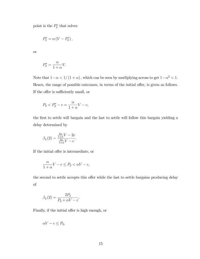
point is the P ∗2 that solves
P ∗2 = α (V − P ∗2 ) ,
or
P ∗2 =α
1 + αV.
Note that 1−α < 1/ (1 + α) , which can be seen by mutliplying across to get 1−α2 < 1.
Hence, the range of possible outcomes, in terms of the initial offer, is given as follows.
If the offer is sufficiently small, or
P2 < P ∗2 − c =α
1 + αV − c,
the first to settle will bargain and the last to settle will follow this bargain yielding a
delay determined by
βb (2) =2α1+α
V − 2c2α1+α
V − c.
If the initial offer is intermediate, or
α
1 + αV − c ≤ P2 < αV − c,
the second to settle accepts this offer while the last to settle bargains producing delay
of
βb (2) =2P2
P2 + αV − c.
Finally, if the initial offer is high enough, or
αV − c ≤ P2,
15

both will accept and there is no delay
βc (2) = 1.
3. Finally, for intermediate levels of c
α2V > c ≥ α2
1 + αV,
the results of a bargain by the first creditor to settle will depend on expectations of
the behavior of the last creditor to settle. Specifically, if it is expected that the next
creditor will follow
P ∗2 =α
1 + αV,
while if it is expected that they will bargain
P ∗2 = α (1− α)V.
The set of possible outcomes, as a function of P2, is analogous to that above except
that there are now multiple equilibria.
Specifically, if the offer is large enough, or
αV − c ≤ P2,
there is no delay as both accept it, or
βc (2) = 1.
If the offer is intermediate, or
α
1 + αV − c ≤ P2 < αV − c,
16

the second to settle follows but last to settle bargains producing delay of
βb (2) =2P2
P2 + αV − c.
For lower P2 we can get multiple equilibria. If
α (1− α)V − c ≤ P2 <α
1 + αV − c,
we get one creditor following and one bargaining, with the identity determined by
expectations (if I expect the last settler to follow, I bargain; if not, I follow and they
bargain). Delay depends on each case.
βb (2) =2P2
P2 + αV − c,
Finally, if
P2 < α (1− α)V − c,
we once again get mutliple equilibria. However, the second last to settle always bar-
gains, while the second may or may not. Depending on expectations, the second last
to settle may negotiate a bigger or smaller payment, which makes the expectations self
enforcing.
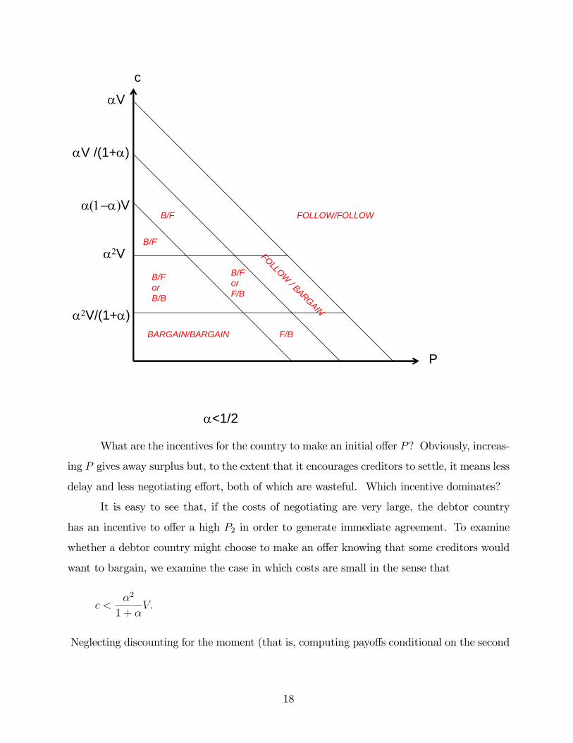
The set of equilibria as a function of c, α and P is displayed in the following figure,
which divides the parameter space. A notation of B/F means that the first to settle
bargains while the second to settle follows (or accepts the same bargain). As shown,
mutliple equilibria only arise for intermediate cost levels.
17
c
P
α<1/2
α2V
α2V/(1+α)
α(1−α)V
αV /(1+α)
αV
FOLLOW/FOLLOW
BARGAIN/BARGAIN
B/F
B/F
F/B
B/F or B/B
B/F or F/B
FOLLOW / BARGAIN
What are the incentives for the country to make an initial offer P? Obviously, increas-
ing P gives away surplus but, to the extent that it encourages creditors to settle, it means less
delay and less negotiating effort, both of which are wasteful. Which incentive dominates?
It is easy to see that, if the costs of negotiating are very large, the debtor country
has an incentive to offer a high P2 in order to generate immediate agreement. To examine
whether a debtor country might choose to make an offer knowing that some creditors would
want to bargain, we examine the case in which costs are small in the sense that
c <α2
1 + αV.
Neglecting discounting for the moment (that is, computing payoffs conditional on the second
18

last creditor settling) we have
V2 (P ) =
⎧⎪⎪⎪⎨⎪⎪⎪⎩(1− α)2 V P < α (1− α)V − c
(1− α)V − P α (1− α)V − c ≤ P < αV − c
V − 2P αV − c ≤ P
Note that
V2 (α (1− α)V − c) = (1− α)2 V + c > V2 (αV − c) = (1− 2α)V + 2c.
Incorporating discounting we get a value function for the debtor of
EV2 (α (1− α)V − c) = βb£(1− α)2 V + c
¤=
£(1− α)2 V + c
¤[2α (1− α)V − 2c]
V (2− α)− 2cEV2 (αV − c) = [(1− 2α)V + 2c]
To find the maximum, we only need worry about choices of P2 that correspond to the local
peaks of this function. To see what may result, suppose we set α = 1/2. Then
EV2 (α (1− α)V − c) =[V/4 + c] [V/2− 2c]
3V/2− 2cEV2 (αV − c) = 2c
Suppose we lower c keeping V constant. The first term stays positive, but the second
approaches zero. Therefore, there must exist c small such that the function EV2 reaches a
maximum at α (1− α)V −c. That is, the country will choose an initial offer in the knowledge
that the last creditor will bargain.
C. An Algorithm For Solving the N Player Game
Equilibria to the game with many players N can be computed using the following
algorithm. At stage two, there may be multiple fixed points corresponding to different ex-
pectations about whether or not future creditors will bargain. The selection at this stage can
have quite substantial effects on the resulting equilibrium.
The algorithm works backwards as follows:
19

1. Begin with V0 (P ) = V.
2. For any value function capturing the surplus to the debtor from future play with n
creditors, Vn (P ) , compute the set of outcomes that would result were the n+1 creditor
to bargain, Pn+1, as the set of values such that
Pn+1 = αVn (Pn+1) .
When there are multiple fixed points, choose largest (or any other rule).
3. Compute the value to the creditor at the time the n + 1 creditor bargains, Vn+1 (P ) ,
as:
Vn+1 (P ) =
⎧⎨⎩ Vn (Pn+1)− Pn+1 Pn+1 > P + c
Vn (P )− P Pn+1 ≤ P + c,
and record the outcome of negotiations
Pn+1 (P ) =
⎧⎨⎩ Pn+1 Pn+1 > P + c
P Pn+1 ≤ P + c
and the payoffs to the n+ 1 creditor who settles as of this point in time
Un+1 (P ) =
⎧⎨⎩ Pn+1 − c Pn+1 > P + c
P Pn+1 ≤ P + c
4. Incorporate discounting to find the cost of delay in determining the identity of the n+1
creditor as
βn+1 (P ) =(n+ 1) Un+1 (P )
Un+1 (P ) + nUn
³Pn+1 (P )
´ ,and the surplus to the debtor at the beginning of the n+ 1 subgame as
Vn+1 (P ) = βn+1 (P ) Vn+1 (P ) .
20

5. Iterate on steps 2 through 5 until n = N − 1.
6. Choose P0 to maximize VN (P ) .
Given the solution to this algorithm, the sequence of settlement payments {Pn}Nn=1 can
be obtained by iterating from P0 with the sequence of functionsnPn
oNn=1
, while the total
cost of delay from negotiations can be computed by multiplying the costs of delay at each
stage. Expected payoffs to the creditors are given as the payoff to the first creditor to settle,
as delay serves to erode any surplus gained by waiting.
D. Calibration
To examine the quantitative implications of our bargaining model, it is necessary that
we take a stand on three main parameters: the bargaining power of the creditors α, the cost of
bargaining c and the number of creditors N.We will attempt to measure the bargaining cost
and power parameters directly and will then experiment with a number of different values
for N to examine the implications of the model for the distribution of default durations.
We begin with the bargaining cost. Inspection of the annual reports of the CFB
indicates that the CFB typically charged bondholders a fee of one-half of one percent of the
face value of any new securities issued in exchange for the old defaulted bonds. However,
this figure probably understates the size of the costs incurred by the CFB as the main office
holders of the Corporation were unremunerated while the CFB also made use of the consular
and diplomatic services of the UK government. Finally, for many years the expenses of the
CFB were directly subsidized by the Bank of England and, under some coercion, by groups
of private banks. Based on these figures, we calibrate an individuals bargaining costs to be
one-half of one per-cent of the total value of the settlement, but also experiment with costs
of bargaining as large as one per-cent of the value of the settlement.
We calibrate our estimates of bargaining power to the differences in settlements re-
ceived by holdouts as opposed to those received by creditors who accepted the exchange offer.
Singh (2003) studies sovereign restructuring negotiations in the 1990s and finds that, when
attention is restricted to debts that were quite liquid and were traded on secondary markets,
21
holdouts averaged returns one and one-half times as large as creditors who accepted an ex-
change offer. This is also the figure estimated by Sturzenegger and Zettelmeyer (2005) in
their study of sovereign debt negotiations, and is the figure most commonly attributed to the
excess return earned by holdouts in US corporate restructurings. Consequently, we set ga to
match this figure.
The final parameter to be calibrated is the number of creditors. This is by far and
away the hardest parameter to calibrate because what is relevant for the model is not the
number of creditors per se, but the effective number in terms of negotiations. The two
can be quite different particularly when bondholdings are quite unequal amongst creditors.
There is also a great deal of dispersion in bondholding levels across recently restructured
bonds. During the 1980’s, bank action committees ranged from having roughly 20 members
all the way up to committes with membershiop of close to one hundred banks and financial
institutions. During the 1990s, some bond restructurings have been conducted with a small
number of institutional investors, while others have involved hundreds of thousands of small
retail investors (in some cases, such as Ukraine, different bonds in the restructuring were held
very differently).
In a number of recent cases of holdout, the mass of holdouts has been equal to roughly
three per-cent of bondholders (although in Argentina’s case, the holdouts were as much as
ten times larger). We will thus experiment with a values of N of 33. This number corresponds
to the assumption that creditors vote in three per-cent blocks.
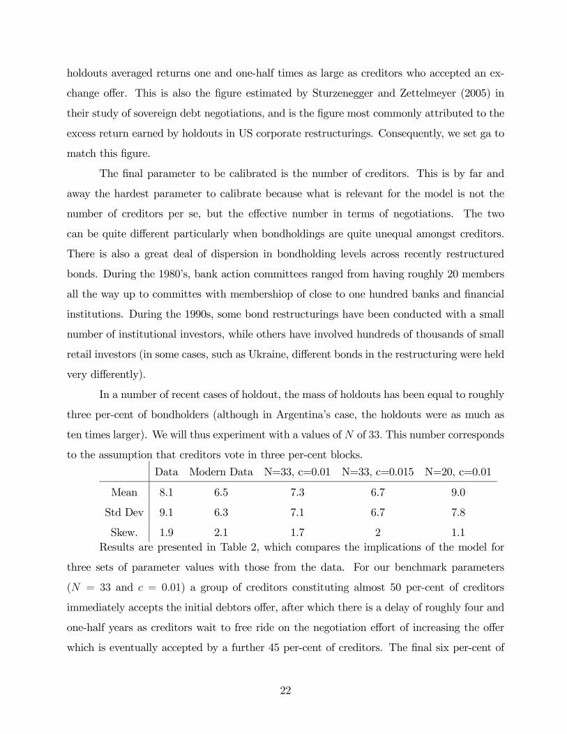
Data Modern Data N=33, c=0.01 N=33, c=0.015 N=20, c=0.01
Mean 8.1 6.5 7.3 6.7 9.0
Std Dev 9.1 6.3 7.1 6.7 7.8
Skew. 1.9 2.1 1.7 2 1.1Results are presented in Table 2, which compares the implications of the model for
three sets of parameter values with those from the data. For our benchmark parameters
(N = 33 and c = 0.01) a group of creditors constituting almost 50 per-cent of creditors
immediately accepts the initial debtors offer, after which there is a delay of roughly four and
one-half years as creditors wait to free ride on the negotiation effort of increasing the offer
which is eventually accepted by a further 45 per-cent of creditors. The final six per-cent of
22

creditors (the “hold outs”) then take another three years to settle.
When bargaining costs are increased by 50%, the debtor responds by increasing the
initial offer. This reduces the incentive for later creditors to renegotiate, although the first
to do so extract a greater settlement. The result is that 40 per-cent of creditors accept the
initial offer, while the remaining 60 per-cent settle after a delay of just under seven years.
Reducing the number of creditors while keeping bargaining costs at one per-cent ef-
fectively reduces the bargaining costs of an individual creditor. In this case, creditors split
into four groups, three of which renegotiate the settlement offer. This leads to substantially
more delay.
E. Intuition for the Results
The results for the first two sets of parameter values, which correspond to our preferred
specifications, are broadly in line with the distribution of delay observed in the data. In this
subsection, we use a simplified version of the timing game to provide intuition for the observed
amount of delay.
There are two main forces governing delay: an incentive to free ride on the negotiation
costs incurred by others; and, an incentive to hold out in the hope of using later veto power
to extract a higher settlement. To understand the quantitative effects of free riding, suppose
that there are N creditors and that the first to settle receives the settlement payment P but
must incur costs c while all other creditors receive the payment P alone. In that case, the
equilibrium of the timing game with symmetric mixed strategies must imply enough delay so
as to make creditors indifferent between following this strategy or settling immediately. That
is, the cost of delay β must satisfy
U − c = βU − c+ (N − 1)U
N,
which can be rearranged ot get
β =N (U − c)
U − c+ (N − 1)U .
23
If we set c = cNU and rearrange we get
β =1− cN
1− c.
For our benchmark parameter c = 0.01, with twenty creditors, this implies a level for β of
about 0.8 which in turn, for standard interest rates, is consistent with a delay of about four
and one-half years.
To understand the effects of holdout on delay, suppose that the first player to settle
receives P while the second group receive P 0. In this case, the cost of delay from hold out
must satisfy
β =MP
P + (M − 1)P 0 =M
1 + (M − 1)P 0/P.
If we set P 0/P = 1.5, consistent with out findings on the returns to hold out discussed above,
and set M = 2 (so that only one player, or about 3 per-cent of creditors, are holdouts) the
implied delay is also on the order of about four and one half years.
Added together, these simple calculations suggest that the forces emphasized above are
capable of producing delays of similar magnitude to thos eobserved in the data. The content
of the bargaining model above is that it determines which of these forces are operative, and
how many creditors are affected.
F. Policy Options To Reduce Delay
Much of the recent debate in policy circles has centered on the proposal to intro-
duce collective action clauses into sovereign bond contracts. This debate appears to have
successfully influenced the practice of sovereign lending beginning with Mexico’s 2003 issue
of sovereign bonds which were amongst the first to be issued under New York Law with
collective action clauses. Over time as the stock of debt is increasingly dominated by debt
containing these clauses, policy makers hope that the length of sovereign bond restructuring
negotiations will decrease. We defer a discussion of the welfare effects of this change until
the next section, when we can consider the effect of these changes on ex ante borrowing. For
24
now we ask: Will this delay? And if so, by how much will delay fall?
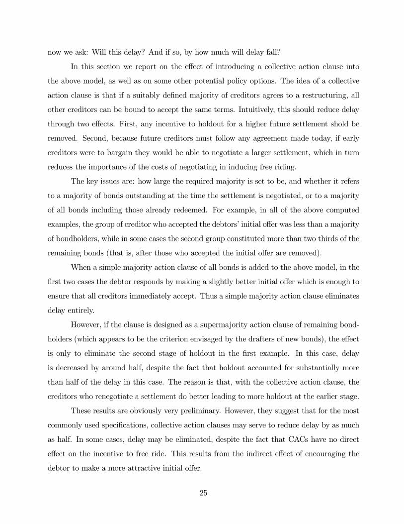
In this section we report on the effect of introducing a collective action clause into
the above model, as well as on some other potential policy options. The idea of a collective
action clause is that if a suitably defined majority of creditors agrees to a restructuring, all
other creditors can be bound to accept the same terms. Intuitively, this should reduce delay
through two effects. First, any incentive to holdout for a higher future settlement shold be
removed. Second, because future creditors must follow any agreement made today, if early
creditors were to bargain they would be able to negotiate a larger settlement, which in turn
reduces the importance of the costs of negotiating in inducing free riding.
The key issues are: how large the required majority is set to be, and whether it refers
to a majority of bonds outstanding at the time the settlement is negotiated, or to a majority
of all bonds including those already redeemed. For example, in all of the above computed
examples, the group of creditor who accepted the debtors’ initial offer was less than a majority
of bondholders, while in some cases the second group constituted more than two thirds of the
remaining bonds (that is, after those who accepted the initial offer are removed).
When a simple majority action clause of all bonds is added to the above model, in the
first two cases the debtor responds by making a slightly better initial offer which is enough to
ensure that all creditors immediately accept. Thus a simple majority action clause eliminates
delay entirely.
However, if the clause is designed as a supermajority action clause of remaining bond-
holders (which appears to be the criterion envisaged by the drafters of new bonds), the effect
is only to eliminate the second stage of holdout in the first example. In this case, delay
is decreased by around half, despite the fact that holdout accounted for substantially more
than half of the delay in this case. The reason is that, with the collective action clause, the
creditors who renegotiate a settlement do better leading to more holdout at the earlier stage.
These results are obviously very preliminary. However, they suggest that for the most
commonly used specifications, collective action clauses may serve to reduce delay by as much
as half. In some cases, delay may be eliminated, despite the fact that CACs have no direct
effect on the incentive to free ride. This results from the indirect effect of encouraging the
debtor to make a more attractive initial offer.
25

Alternative policy options are available. One option that received a lot of attention
during Argentina’s recent restructuring are the so called “most favored creditor clauses”. In
principle, these clauses entitle creditors who have settled at an earlier stage to receive any
more favorable payment that is negotiated at a later stage. In the case of Argentina, the
language of the clause appeared to explicitly exclude settlement offers of this sort. However,
there appears to be no reason in principle why clauses could have been written to include
settlements. In this case, the details of the majority and how it is determined are irrelevant.
Delay may not be eliminated, however, if the debtors initial offer is not high enough to deter
all renegotiation.
Finally, one can imagine schemes in which the costs of negotiations are shared amongst
all creditors thus removing the incentive to free ride. One such scheme would be the rein-
troduction of bondholder representative groups such as the CFB. If CFB agreements were
considered to be binding on all creditors, holdout would also be eliminated, and hence all
delay could be avoided. Whether or not this would be a desirable outcome depends upon the
effects of eliminating or reducing the default penalty on the ability of the debtor country to
borrow in normal times. To address this question directly, we turn to a model of borrowing
in the next section.
4. Borrowing Environment
In this section, we outline the main aspects of our economic environment. A sovereign
country borrows from competitive international financial intermediaries to finance a periodi-
cally recurring investment project. The sovereign cannot commit to repay these borrowings
and may default on what is otherwise a state non-contingent debt contract. The consequences
of default are a period of lost access to international financial markets, and a financial set-
tlement. In this section, we treat both the period of lost access and the size of the financial
settlement as parameters. In the next section, we go on to endogenize these variables as the
result of an explicit bargaining game.
26

A. The Basic Model
Time evolves continuously and last forever. However, investment projects take discrete
amounts of time which give the model the flavor of a discrete time model. At any point in time
t in which a sovereign country is not engaged in an investment project, the sovereign country
has access to a production opportunity that requires foreign capital. We assume that the
project requires a fixed k units of capital from abroad6. Both the sovereign country, and all
international creditors are risk neutral, and both discounts the future at the world interest rate
rW . Note that the only motive for borrowing is to finance the investment opportunity; both
the creditors and the sovereign borrower are risk neutral and discount the future identically7.
It will be convenient to denote by δ the discount factor that applies to points in time one
unit apart
δ =1
RW= e−r
wtdt.
After capital has been borrowed, a discrete unit of time passes, which we normalize
to one unit, before the sovereign debtor observes the productivity level of the project that
period θ. This is the only source of uncertainty in the model. At this point, the sovereign
debtor may decide whether or not to default. If the debtor does not default, the capital is
committed to the project and the country receives any output plus undepreciated capital of
θf (k) + (1− d) k net of any interest payments contracted on the debt Rk, where f (k) is
a standard neoclassical production function and R > RW is the gross rate of interest on a
state non-contingent sovereign bond which is determined endogenously as shown below. In
addition, if the country repays its debts, it is free to borrow again next period.
Should the country decide to default, they are able to appropriate the undepreciated
capital stock (1− d) k and do not have to pay back any interest on the loan this period. Next
6This assumption is for tractability. It comes at the cost of limiting the intensive margin of productionalong which changes in the international financial architecture can affect the level of production within acountry (the only choice for the country is now whether to produce or not, and not how much to produce).This lowers the cost of default in the model because, if investment was flexible, default risk would lead tohigher interest rates and lower investment levels. on the margin.
7The assumption that the country is risk neutral reduces the benefits of default by eliminating any sensein which default provides insurance against consumpiton fluctuations. Default does provide insurance againstlow realizations of the productivity shock in production.
27

period, however, they will have to enter renegotiations with creditors8. For the entirety of
this section, we model the outcome of this renegotiation process in a reduced form fashion
summarized by three parameters β, P and λ that serve to capture any delay in negotiations,
as well as the size of any settlement payment made by the debtor at the time of the settlement,
and any resources used up in negotiations. More explicitly, the parameter β serves to capture
the expected cost of delay resulting form the renegotiation process that defers the point at
which the country is able to re-access capital markets. Similarly, the parameter P captures
the expected level of the settlement payment made by the debtor at this future date, while λP
is the amount received by the creditor. We assume that the discounted value of a settlement
is less than what would have been earned has the capital been invested in the risk free security
βλP < RWk.
If we let V 0 denote the value to the country from re-accessing capital markets in the
future, then it is easy to see that the country will default whenever
θf (k) + (1− d−R) k + δV 0 < (1− d) k + δβV 0 − βP.
This can be rearranged to show that a country will default whenever the productivity shock
is sufficiently low, or
θ <Rk − (1− β) δV 0 + βP
f (k)≡ θ∗ (k) .
That is, the productivity shock must drop lower than the interest rate on sovereign loans
by an amount at least as large as the discounted future costs of default. This has two
components: a pure cost of delay which reduces the value of future credit market access by
a factor of (1− β) ; and, any future settlement payments that occur at a later date. We let
8We use the term “enter negotiations” to signify that the debtor moves into the renegotiation game.Of course, one possible outcome of this game is that the debtor and creditors do not begin negotiationsimmediately.
28

the probability of default be denoted by
π (k) = Pr {θ < θ∗ (k)} .
International creditors are risk neutral and competitive expecting to earn zero profits
in equilibrium. This requires that the weighted average of returns with and without a default
be equal to the world interest rate, or
¡1 + rW
¢k = (1− π)Rk + πβλP,
which can be rearranged to give an expression for the interest rate on sovereign bonds of
R =1 + rW − πβλP/k
1− π.
As creditors make zero profits, world welfare in this economy is given purely by the
welfare of the country, which in expected value terms is given by
V = (1− π) [E [θ|θ ≥ θ∗ (k)] f (k) + (1− d) k −Rk + δV 0] + π [(1− d) k + β (δV 0 − P )]
= (1− π)E [θ|θ ≥ θ∗ (k)] f (k) + (1− d) k −RWk + [1− π (1− β)] δV 0 − πβ (1− λ)P.
This can be contrasted with a world in which sovereign debtors could commit to honoring
contracts (but are constrained to have the same future value of access to capital markets).
V C =¡E [θ] f (kc) + (1− d) kc −RW
¢k + δV 0,
where we have used kc to denote the fact that the level of capital chosen in this full commit-
ment environment will typically differ from that chosen when a country can default. Note
that
V − V C = [(1− π)E [θ|θ ≥ θ∗ (k)] f (k)−E [θ] f (kc)]
+£1− d−RW
¤(k − kc)− π (1− β) δV 0 − πβ (1− λ)P.
29

Approximating f (kc) around k, we get
V − V C ' [(1− π)E [θ|θ ≥ θ∗ (k)]− E [θ]] f (k)
+£E [θ] f 0 (k)−
¡d+ rW
¢¤(k − kc)− π [(1− β) δV 0 − β (1− λ)P ] .
The first term represents the loss of output that occurs when the country diverts
capital. Note that this may be negative (and hence default has the potential to be welfare
improving) if low enough realizations of the productivity shock are allowed; it is in this sense
that allowing default completes markets and allows the world to minimize risk. A decrease
in default penalties has the potential to either increase or decrease this term.
The second term captures the effect of changing default risk on the amount of capital
borrowed. If under default risk, less capital is borrowed than with full commitment, the first
part of this term is positive while the second is negative, reflecting the fact that the world
loses when less than the optimal amount of capital is borrowed. Decreasing default penalties
will make this term more negative.
The third term corresponds to the fact that default occurs in equilibrium and is costly
in terms of delay and resource usage: with probability π, the country loses the fraction
(1− β) of future value δV 0 through delay, and loses the (1− λ)P of resources in the future.
Decreasing these costs will raise world welfare as long as the probability of default does not
rise too fast.
Note that the overall term is not obviously positive or negative: default may produce
a benefit in terms of being able to truncate the distribution of shocks to production; however,
this comes at the cost of placing positive probabilities on the occurrence of costly defaults
which also implies a higher interest rate. Similarly, policy reforms that facilitate debt restruc-
turings and lower delay (raise β) may either raise or lower welfare. Essentially, as β rises,
delay falls. But this will lead to an increased default probability, and further truncation of
the distribution of realized productivity shocks.
Obviously, if full commitment dominated default, this effect will be magnified through
the value of future interactions in this environment. However, the resulting welfare compar-
ison consists of the same components as the expression derived above, with some elements
30

magnified because of the fact that they are incurred every period with positive probability.
B. Solution Algorithm
As a result of our assumptions on production and risk neutrality, the model above has
only two non-linear components: the probability of default, and the expectation of produc-
tivity conditional on repayment. In the next section we show how, by assuming a uniform
distribution on shocks, we can make the model entirely linear and solve it using pencil and
paper methods. In this section, we outline ways to think about the solution of the model
more generally.
Imposing the assumption that the economy is stationary so that V 0 = V, the equilib-
rium of our economy can be reduced to two equations. The first gives us the value to the
country as a function of the conditional expectation of productivity and the probability of
default, as
V =(1 + (1− π)E [θ|θ ≥ θ∗])−RW
1− [1− π (1− β)] δk.
The second is simply the productivity of default
π = Pr {θ < θ∗}
= Pr
½θ < R− (1− β) δV + βP
k
¾= Pr
½θ <
RW − βP/k − (1− π) (1− β) δV/k
1− π
¾,
where it is important to note that π also affects the endogenous interest rate on borrowings.
There are two routes to solving the model. First, once can postulate a functional form
for the distribution of productivity shocks θ, f (θ) , and then solve the model directly. We
have pursued this approach in other work.
Second, one can solve the model numerically using recursive methods. One algorithm
that works first reformulates the model in terms of the price of debt q = 1/R. Under our
assumptions, q is bounded below by zero, and above by 1/RW , unlike R which may be
unbounded above. The algorithm proceeds by iterating on two operations or mappings. The
31

first operation, takes as given the value of q, say qn, and is used to compute the corresponding
value to the country Vn as a fixed point. We denote this mapping by T Vn where the n serves
to denote that the mapping is defined for qn as given
T Vn (V ) = max
x∈{0,k}E {max {(1 + θ − 1/qn)x+ δV, x+ β (δV − P )}} .
It is straightforward to see that this is a contraction mapping on the real numbers. Let the
fixed point of this mapping be denoted by Vn.
The second operation acts on the interest rate by first updating the probability of
default given the fixed point of the first mapping
πn+1 = Pr
½θ <
1
qn− (1− β) δVn + βP
k
¾,
which leads then to a new bond price
qn+1 =1− πn+1
RW − πn+1βP/k.
We let this mapping on the bond prices q be denoted by T q. We can then show that this
iteration of mappings produces a monotone sequence for the bond prices.
Proposition 1. If q0 < q then T q (q0) ≤ T q (q) .
Proof. Let q0 ≤ q. Then the fixed point of the operator T V defined for q0 is weakly less than
the one for q, or V 0 ≤ V, because the period return function is smaller. But then
π (q0) = Pr
½θ <
1
q0− (1− β) δV 0 + βP
k
¾≥ Pr
½θ <
1
q0− (1− β) δV + βP
k
¾≥ Pr
½θ <
1
q− (1− β) δV + βP
k
¾= π (q) ,
which implies that
T q (q0) ≤ T q (q) .
32

As q is bounded below, this implies that an equilibrium exists. We do not know that
it is unique. Intuitively, a higher interest rate makes default more likely which can justify a
higher interest rate in equilibrium, so that the possibility for multiple equilibria exist.
C. Numerical Results
In this subsection, we explore the implications of introducing CACs to our benchmark
bargaining model, and then introducing this change to our model of borrowing.
Most of the parameters for the model are set to standard values. The annual world
interest rate is set to 5%, with depreciation at 8.5%. The production function is assumed
to have an output elasticity of one third. One of the more important magnitudes involves
the “shape” and “location” of the productivity shock distribution. We use data from Tomz
and Wright (2007) covering 175 countries at annual frequencies for up to 180 years on the
evolution of output in both default and non-default years to construct an empirical density
for the level of productivity shocks. This gives us the shape of the distribution. The mean
of the distribution, and a scale factor governing its standard deviation are then set to match
two parameters: a default probability of 2% in the benchmark model, and a mean output
cost of 2% as estimated by Chuhan and Sturzenegger (2005).
We begin with the benchmark model and examine the introduction of collective action
clauses, which we saw above had the effect of reducing delay by about half from just under
seven years to about 3.5 years. The model finds that this has the effect of increasing welfare
by about six hundredths of one per-cent of GDP per year. This is a tiny amount.
To get a handle on why this is the estimated benefit, note that in the benchmark
model a country defaults on average twice per century and when it does, it loses two per-cent
of GDP per year for about 7 years. Roughly speaking, it loses about 0.28% of GDP of annual
GDP. When CACs are introduced, a country now loses only 2% of GDP for about 3,5 years,
but it now does so about 25% more often, defaulting on average 2.5 times per century. That
is, it now loses about 0.2% of annual GDP from defaults. However, this gain is offset by
the fact that the country now pays a higher interest rate in normal times, which leads it
33

to borrow about 3% less on average. Given an output elasticty of 1/3, this implies 1% less
output from foreign borrowing per year for about 90 years in every century. The result is a
net increase in output of only 6 hundredths of one per-cent of GDP.
Obviously, these results depend on the estimated shape of the productivity distribution
which determines the change in the probability of default. This is something about which
we have only limited confidence. To put it another way, one can ask: how large would the
increase in default probabilities have to be eliminate any welfare increase at all? One can
reverse engineer the model to show that default probabilities would have to rise to a level
implying 3.5 defaults every century. This seems like an implausibly large number, which leads
us to be confidence in the direction of the change: the introduction of CACs should increase
welfare.
What about the quantitative magnitudes? This result seems startlingly small relative
to some of the proposed claims of benefits from reform of the SDRM. It is also, no doubt,
sensitive to the exact specification of the borrowing model. Nonetheless, the basic logic would
seem to be robust: since defaults are rare events, they will have only a small effect on welfare.
Obviously, our conclusions change if we condition upon being in a default, if we increase
the estimate of the output cost of default (for example, Eichengreen 2002 examines estimates
four to five times larger than the one we consider) or consider changes with transfer bargaining
power to creditors thus increasing the incentives of countries to repay while also substantially
reducing social waste. Preliminary estimates suggest that the benefit of introducing a veto
option proposal as outlines above suggest a welfare gain of about one half of one percent of
annual GDP. We intend to refine this estimate in future work.
5. Conclusion
This paper has presented a theory of the process by which sovereign countries in
default restructure their debts with private creditors. We have found that the observed delay
in restructuring negotiations can plausibly be explained by a combination of free riding on
negotiation effort with an incentive to holdout to obtain better settlement terms. These
findings imply that current options aimed at reducing delay, such as collective action clauses,
have the potential to reduce but not eliminate the observed delays in debt restructuring.
34
This positive model of the bargaining process was then combined with a model of
sovereign borrowing to examine the normative question of whether or not these reductions
in delays are welfare improving. We find they are not, and further that the optimal level
of delay would plausibly involve an increase over current levels. The logic seems robust to
various changes in the modeling framework: essentially, defaults are sufficiently rare events
that the benefits from reducing the costs of a default ex post are small relative to the gains
associated with reducing borrowing costs, and thus increasing borrowing levels, in normal
times.
The model and analysis of this paper could usefully be extended in a number of
directions. Empirically, our examination of default duration has focused on the amount of
time between the beginning of a default and its end defined as the time at which a majority
of creditors agree to a settlement. In practice, as well as in the context of our model, a more
appropriate definition would involve defining the end of the default as the first date at which
a country is able to reaccess international capital markets. Work on this question for the
modern period, relying on data on gross capital flows, has been conducted by Gelos, Sahay
and Sandleris (2004), and using data on net cpaital flows by Miller, Tomz and Wright (2005)
and Richmond (2007).
Theoretically, our model points to some subtle incentives facing countries and creditor
with respect to the design of debt contracts. On the one hand, a country gains ex ante by
designing contracts so that they are costly to restructure ex post. On the other, increasing
the costs of bargaining directly can perversely lead to a reduction in the costs of restructuring
debts, as higher costs bind future creditors to accept settlements negotiated by creditors that
have settled earlier in the restructuring process, leading to shorter delays and higher returns
to the country. Consequently, reducing the costs of bargaining by making debts easier to
restructure, can somewhat surprisingly lead to more diversity amongst settlements and more
delay as creditors sort themselves into different settlement groups.
Our model also emphasizes that the most efficient way to deter default is to increase
the bargaining power of creditors in the event of a default restructuring. Such increases
reduce the incentives of a country to default without wasting social surplus. Some modest
changes to the debt restructuring process present themselves. One possibility is to design
35
what we refer to as a veto option proposal in which the first creditor to negotiate offers the
debtor an option to buy its outstanding debt (that creditors veto power) that only vests if
all creditors simultaneously sell seimilar options. If this offer is rejected, negotiations wqould
resume in the old debt restructuring regime. The costs of the first creditor to negotiate would
be fully subsidized by the IMF. In such a world, there would be no delay and hence litrle
socialsurpluis wasted, while the country would continue to receive the same payoffs as in the
old regime and hence facing the same incentives to repay. Indeed, and somewhat surprisingly,
the outcome of this veto option proposal would be further strengthened if the old regime was
modified to further increase delays and hence further lower debtor country payoffs.
36
References[1] Abreu, Dilip and Faruk Gul. 2000. "Bargaining and Reputation." Econometrica, 68:1,
pp. 85-117.
[2] Aguiar, Mark and Gita Gopinath. 2006. "Defaultable Debt, Interest Rates and the Cur-
rent Account." Journal of International Economics, 69:1, pp. 64-83.
[3] Alesina, Alberto & Drazen, Allan, 1991. “Why Are Stabilizations Delayed?” American
Economic Review, American Economic Association, vol. 81(5), pages 1170-88, December.
[4] Alfaro, Laura. (2006). “Creditor Activism in Sovereign Debt: “Vulture” Tactics or Mar-
ket Backbone.” Harvard Business School Case 9-706-057.
[5] Arraiz, Irani (2006). “Default, Settlement, and Repayment History: A Unified Model of
Sovereign Debt,” Unpublished paper, University of Maryland.
[6] Arellano, Cristina. 2006. "Default Risk and Income Fluctuations in Emerging
Economies." University of Minnesota Working Paper.
[7] Bolton, Patrick and Olivier Jeanne (2005) “Structuring and Restructuring Sovereign
Debt: The Role of Seniority,” National Bureau of Economic Research Working Paper
11071.
[8] Jeremy Bulow & Paul Klemperer, 1999. “The Generalized War of Attrition,” American
Economic Review, American Economic Association, vol. 89(1), pages 175-189, March.
[9] Dooley, Michael P. (2000) “International Financial Architecture and Strategic Default:
Can Financial Crises Be Less Painful?” Carnegie-Rochester Conference Series on Public
Policy, Volume 53, Issue 1, December 2000, Pages 361-377.
[10] Eichengreen, Barry and Richard Portes (1995), Crisis? What Crisis? Orderly Workouts
for Sovereign Debtors, London: Centre for Economic Policy Research.
[11] Eichengreen, Barry (2002), Financial Crises and What to Do About Them, Oxford:
Oxford University Press.
37
[12] Eichengreen, Barry and Richard Portes (1989), “After the Deluge: Default, Negotiation
and Readjustment during the Interwar Years,” in Barry Eichengreen and Peter Lindert
(eds), The International Debt Crisis in Historical Perspective, Cambridge, Mass.: MIT
Press, pp.12-47.
[13] Fernández, Raquel and Jacob Glazer. 1991. "Striking for a Bargain between Two Com-
pletely Informed Agents." American Economic Review, 81:1, pp. 240-52.
[14] Fernández, Raquel and Robert W. Rosenthal. 1988. "Sovereign-debt renegotiations : a
strategic analysis." NBER Working Paper, 2597, pp. 20.
[15] Fernández-Arias, Eduardo. 1991. "A dynamic bargaining model of sovereign debt."
World Bank Policy Research Working Paper Series, 778.
[16] Hendricks, Ken, Andrew Weiss, and Charles Wilson. 1988. "The War of Attrition in
Continuous Time with Complete Information." International Economic Review, 29:4,
pp. 663-80.
[17] International Monetary Fund (2003). Reviewing the Process for Sovereign Debt Restruc-
turing within the Existing Legal Framework, International Monetary Fund.
[18] Krueger, Anne O. (2001). “A New Approach to Sovereign Debt Restructuring.” Ad-
dress to Indian Council for Research on International Economic Relations, Delhi, India,
December 20, http://www.imf.org/external/np/speeches/2001/112601.htm.
[19] Krueger, Anne O. (2002). “Sovereign Debt Restructuring Mechanism-One Year
Later.” Address to European Commission, Brussels, Belgium, December 10,
http://www.imf.org/external/np/speeches/2002/121002.htm.
[20] Krueger, Anne O. (2002). A New Approach to Sovereign Debt Restructuring. Interna-
tional Monetary Fund.
[21] Livshits, Igor, James MacGee, and Michele Tertilt. 2006. "Consumer Bankruptcy: A
Fresh Start." University of Western Ontario Working Paper.
38

[22] Maurer, Noel and Aldo Mussacchio (2006). “The Barber of Buenos Aires: Argentina’s
Debt Renegotiation.” Harvard Business School Case 9-706-034.
[23] Miller, David A., Michael Tomz and Mark L. J. Wright (2005) “Sovereign Debt, Default
and Bailouts,” Stanford University Working Paper.
[24] Rubinstein, Ariel 1982. "Perfect Equilibrium in a Bargaining Model." Econometrica,
50:1, pp. 97-110.
[25] Taylor, John B. (2002) “Sovereign Debt Restructuring: A U.S. Per-
spective.” Remarks at the Conference “Sovereign Debt Workouts: Hopes
and Hazards?”, Institute for International Economics, Washington, D.C,
http://www.ustreas.gov/press/releases/po2056.htm.
[26] Tomz, Michael and Mark L.J. Wright (2006) “Do Countries Default in ‘Bad Times’?”
Journal of the European Economic Association, forthcoming.
[27] Yue, Vivian Z. (2005). “Sovereign Default and Debt Renegotiation,” NYU Working
Paper.
39

-2%
-1%
0%
1%
2%
3%
4%
1994
1995
1996
1997
1998
1999
2000
2001
2002
2003
2004
% G
NI
Net Resource Flows
Net Resource Transfers
Argentine Sovereign Capital Flows
40

t t’
Observe θ
Default/Repay
Consume
Borrow kRepay
Default
Borrow k
Borrow kRestructuring Negotiations
Settle P
β δδ
δ
41


