arX
iv:q
uant
-ph/
0512
209v
1 2
2 D
ec 2
005 Quantum Computation, Complexity, and
Many-Body Physics
Rolando D. Somma
Instituto Balseiro, S. C. de Bariloche, Argentina, and Los Alamos NationalLaboratory, Los Alamos, USA.
August 2005
Dr. Gerardo OrtizPhD Advisor

2

To Janine and Isabel

Abstract
By taking advantage of the laws of physics it is possible to revolutionize the waywe communicate (transmit), process or even store information. It is now knownthat quantum computers, or computers built from quantum mechanical elements,provide new resources to solve certain problems and performcertain tasks moreefficiently than today’s conventional computers. However,on the road to a com-plete understanding of the power of quantum computers thereare intermediatesteps that need to be addressed. The primary focus of this thesis is the under-standing of the possibilities and limitations of the quantum-physical world in theareas of quantum computation and quantum information processing.
First I investigate the simulation of quantum systems on a quantum computer(i.e., a quantum simulation) constructed of two-level quantum elements or qubits.For this purpose, I present algebraic mappings that allow one to efficiently ob-tain physical properties and compute correlation functions of fermionic, anyonic,and bosonic systems with such a computer. By studying the amount of resourcesrequired for a quantum simulation, I show that the complexity of preparing a quan-tum state which contains the desired information is crucialat the time of evalu-ating the advantages of having a quantum computer over a conventional one. Asa small-scale demonstration of the validity of these results, I show the simulationof a fermionic system using a liquid-state nuclear magneticresonance (NMR) de-vice.
Remarkably, the conclusions obtained in the area of quantumsimulations canbe extended to general quantum computations by means of the notion of gen-eralized entanglement. This is a generalization based on the idea that quantumentanglement (i.e., the existence of non-classical correlations) is a concept thatdepends on the accesible information, that is, relative to the observer. Then Ipresent a wide class of quantum computations that can be efficiently simulatedon a conventional computer and where quantum computers cannot be claimed tobe more powerful. The idea is that a quantum algorithm, performed by applying

ii
a restricted set of gates which do not create generalized entangled states relativeto small (polynomially-large) sets of observables, can be imitated using a similaramount of resources with a conventional computer. However,a similar statementcannot be obtained when generalized entangled states (relative to these sets) areinvolved, because this purely quantum phenomena cannot be easily reproducedby classical-information methods.
Finally, I show how these concepts developed from an information-theorypoint of view can be used to study other important problems inmany-body physics.To begin with, I exploit the notion of Lie-algebraic purity to identify and charac-terize the quantum phase transitions present in the Lipkin-Meshkov-Glick modeland the spin-1/2 anisotropic XY model in a transverse magnetic field. The resultsobtained show how generalized entanglement leads to usefultools for distinguish-ing between ordered and disordered phases in quantum systems. Moreover, I dis-cuss how the concept of general mean field hamiltonians naturally emerges fromthese considerations and show that these can be exactly diagonalized by using aconventional computer.
In brief, in this thesis I apply several topics developed in the context of quan-tum information theory to study the complexity of obtainingrelevant physicalproperties of quantum systems with a quantum computer, and to study differentphysical processes in quantum many-body systems.
Acknowledgements
Many people have contributed in one way or another to my PhD thesis. With-out them, this work would have been impossible. It is time then, to express mygratitude to each one who participated in this long journey.
I would first like to thank my family, starting with a special thanks to mywife Janine and our little miracle Isabel, for bringing happiness every morning,which allows me to enjoy and continue with this life. Also, I’m very thankful tomy parents and siblings for their limitless support and for having provided andsustained the basis that guides me every day. Only God can explain how much Ilove everyone of them.
On the scientific side, I want to give special thanks to my PhD advisor andfriend, Dr. Gerardo Ortiz, for his dedication and for givingme the tools to realizethis work. His constant help, teachings, and his own personal passion for sciencehave been the main reasons for my achievements during this time as a PhD student.
Also, I’m very thankful to everyone in the quantum information group at LosAlamos National Laboratory for sharing their knowledge andfor their dedication.They are the reason for many important results obtained in this thesis. In partic-ular, I want to thank my collaborators Howard Barnum, Many Knill, RaymondLaflamme, Camille Negrevergne, and Lorenza Viola, for theirhelp and contribu-tions. Throughout my years at Los Alamos, they have treated me as an equal as ascientist, something that is priceless.
In the same way, I want to thank my professors and administrators at the In-stituto Balseiro that, although most of my PhD studies were not performed inArgentina, they were a constant source of support. In particular, I want to thankDr. Armando A. Aligia for having helped me in many scientific and pedagogicalaspects of this thesis. Also, I want to thank Carlos Balseiro, Raul Barrachina,Manuel Caceres, Daniel Domınguez, Jim Gubernatis, Armando F. Guillermet,Karen Hallberg, Eduardo Jagla, Lisetta, Marcela Margutti,Hugo Montani andJuan Pablo Paz. Each one of them has contributed in one way or another to this

iv
work.Finally, I want to thank Andres, Seba, Sequi, the ‘star team’, and all my friends
from Buenos Aires and Bariloche, and the Ortiz, the Batistas, the Dalvits, theMachados, and every member of the Argentinean community in New Mexico.Through their support and sense of humor, we have entertained ourselves over theyears.

Contents
1 Introduction 1
2 Simulations of Physics with Quantum Computers 92.1 Models of Quantum Computation . . . . . . . . . . . . . . . . . 11
2.1.1 The Conventional Model of Quantum Computation . . . . 112.1.2 Hamiltonian Evolutions . . . . . . . . . . . . . . . . . . 172.1.3 Controlled Operations . . . . . . . . . . . . . . . . . . . 18
2.2 Deterministic Quantum Algorithms . . . . . . . . . . . . . . . . 202.2.1 One-Ancilla Qubit Measurement Processes . . . . . . . . 212.2.2 Quantum Algorithms and Quantum Simulations . . . . . . 22
2.3 Quantum Simulations of Quantum Physics . . . . . . . . . . . . . 252.3.1 Simulations of Fermionic Systems . . . . . . . . . . . . . 252.3.2 Simulations of Anyonic Systems . . . . . . . . . . . . . . 302.3.3 Simulations of Bosonic Systems . . . . . . . . . . . . . . 31
2.4 Applications: The 2D fermionic Hubbard model . . . . . . . . .. 372.5 Quantum Algorithms: Efficiency and Errors . . . . . . . . . . . .392.6 Experimental Implementations of Quantum Algorithms . .. . . . 42
2.6.1 Liquid-State NMR Quantum Information Processor . . . .422.7 Applications: The Fano-Anderson Model . . . . . . . . . . . . . 46
2.7.1 Experimental Protocol and Results . . . . . . . . . . . . . 512.8 Summary . . . . . . . . . . . . . . . . . . . . . . . . . . . . . . 54
3 Quantum Entanglement as an Observer-Dependent Concept 593.1 Quantum Entanglement . . . . . . . . . . . . . . . . . . . . . . . 63
3.1.1 Separability and von Neuman Entropy . . . . . . . . . . . 643.1.2 Mixed-State Entanglement and the Concurrence . . . . . 663.1.3 Measures of Quantum Entanglement . . . . . . . . . . . . 67
3.2 Generalized Entanglement . . . . . . . . . . . . . . . . . . . . . 68

vi CONTENTS
3.2.1 Generalized Entanglement: Definition . . . . . . . . . . . 683.2.2 Generalized Entanglement and Lie Algebras . . . . . . . 693.2.3 Generalized Entanglement and Mixed States . . . . . . . 73
3.3 Relative Purity as a Measure of Entanglement in Quantum Systems 743.3.1 Two-Spin Systems . . . . . . . . . . . . . . . . . . . . . 743.3.2 N-Spin Systems . . . . . . . . . . . . . . . . . . . . . . 783.3.3 Fermionic Systems . . . . . . . . . . . . . . . . . . . . . 79
3.4 Summary . . . . . . . . . . . . . . . . . . . . . . . . . . . . . . 81
4 Generalized Entanglement as a Resource in Quantum Information 834.1 Quantum Entanglement and Quantum Information . . . . . . . .84
4.1.1 Quantum Cryptography . . . . . . . . . . . . . . . . . . 844.1.2 Quantum Teleportation . . . . . . . . . . . . . . . . . . . 86
4.2 Quantum Entanglement and Quantum Computation . . . . . . . .874.3 Efficient Classical Simulations of Quantum Physics . . . .. . . . 91
4.3.1 Higher Order Correlations . . . . . . . . . . . . . . . . . 954.4 Generalized Entanglement and Quantum Computation . . . .. . 97
4.4.1 Efficient Initial State Preparation . . . . . . . . . . . . . . 984.5 Summary . . . . . . . . . . . . . . . . . . . . . . . . . . . . . . 100
5 Generalized Entanglement and Many-Body Physics 1015.1 Entanglement and Quantum Phase Transitions . . . . . . . . . .. 102
5.1.1 Lipkin-Meshkov-Glick Model . . . . . . . . . . . . . . . 1045.1.2 Anisotropic XY Model in a Transverse Magnetic Field . .110
5.2 General Mean-Field Hamiltonians . . . . . . . . . . . . . . . . . 1205.2.1 Diagonalization Procedure . . . . . . . . . . . . . . . . . 1225.2.2 Example: Fermionic Systems . . . . . . . . . . . . . . . 127
5.3 Summary . . . . . . . . . . . . . . . . . . . . . . . . . . . . . . 128
6 Conclusions 1296.1 Future Directions . . . . . . . . . . . . . . . . . . . . . . . . . . 133
A Discrete Fourier Transforms 135
B Discrete Fourier Transform and Propagation of Errors 137
C The Adjoint Representation 139
D Separability, Generalized Unentanglement, and Local Purities 143
CONTENTS vii
E Approximations of the exponential matrix 147E.1 Scaling of the Method . . . . . . . . . . . . . . . . . . . . . . . . 151
F Efficient Classical Evaluation of High-Order Correlation Functions 153
G Classical Limit in the LMG Model 159

Chapter 1
Introduction
...there is plenty of room to make computers smaller...nothing that Ican see in the physical laws...
R. P . Feynman, Caltech (1959).
During the last few decades, the theory of Quantum Information Processing(QIP) has acquired great importance because it has been shown that informationbased on quantum mechanics provides new resources that go beyond the tradi-tional ‘classical information’. It is now known that certain quantum mechanicalsystems, named quantum computers (QCs), can be used to easily solve certainproblems which are difficult to solve using today’s conventional or classical com-puters CCs. Having a QC would allow one to communicate in secret [BB84](quantum cryptography), perform a variety of search algorithms [Gro97], factorlarge numbers [Sho94], or simulate efficiently some physical systems [OGK01,SOG02]. Additionally, it would allow us to break security codes used, for ex-ample, to secure internet communications, optimize a largevariety of schedulingproblems, etc., which make of quantum information an exciting and relevant sub-ject. Consequently, the science of quantum information is mainly focused on bet-ter understanding the foundations of quantum mechanics (which are different ofclassical mechanics) and the physical realization of quantum controllable physicaldevices. While the first allows clever and not so obvious waysof taking advantageof the quantum world, the latter will let us achieve our most important goal: thebuilding of a QC.
When one looks for the wordinformationin the dictionary one finds many def-initions: i) a message received and understood, ii) knowledge acquired through
2 Introduction
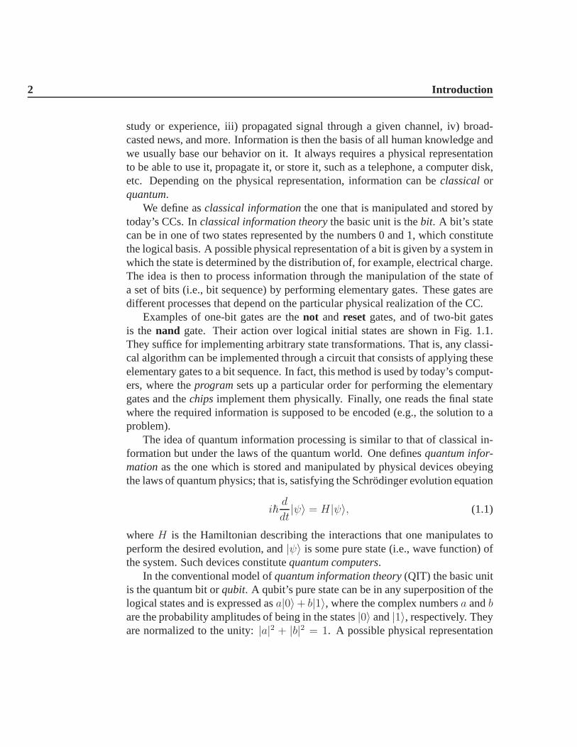
study or experience, iii) propagated signal through a givenchannel, iv) broad-casted news, and more. Information is then the basis of all human knowledge andwe usually base our behavior on it. It always requires a physical representationto be able to use it, propagate it, or store it, such as a telephone, a computer disk,etc. Depending on the physical representation, information can beclassicalorquantum.
We define asclassical informationthe one that is manipulated and stored bytoday’s CCs. Inclassical information theorythe basic unit is thebit. A bit’s statecan be in one of two states represented by the numbers 0 and 1, which constitutethe logical basis. A possible physical representation of a bit is given by a system inwhich the state is determined by the distribution of, for example, electrical charge.The idea is then to process information through the manipulation of the state ofa set of bits (i.e., bit sequence) by performing elementary gates. These gates aredifferent processes that depend on the particular physicalrealization of the CC.
Examples of one-bit gates are thenot and reset gates, and of two-bit gatesis thenand gate. Their action over logical initial states are shown in Fig. 1.1.They suffice for implementing arbitrary state transformations. That is, any classi-cal algorithm can be implemented through a circuit that consists of applying theseelementary gates to a bit sequence. In fact, this method is used by today’s comput-ers, where theprogramsets up a particular order for performing the elementarygates and thechipsimplement them physically. Finally, one reads the final statewhere the required information is supposed to be encoded (e.g., the solution to aproblem).
The idea of quantum information processing is similar to that of classical in-formation but under the laws of the quantum world. One definesquantum infor-mationas the one which is stored and manipulated by physical devices obeyingthe laws of quantum physics; that is, satisfying the Schrodinger evolution equation
i~d
dt|ψ〉 = H|ψ〉, (1.1)
whereH is the Hamiltonian describing the interactions that one manipulates toperform the desired evolution, and|ψ〉 is some pure state (i.e., wave function) ofthe system. Such devices constitutequantum computers.
In the conventional model ofquantum information theory(QIT) the basic unitis the quantum bit orqubit. A qubit’s pure state can be in any superposition of thelogical states and is expressed asa|0〉+ b|1〉, where the complex numbersa andbare the probability amplitudes of being in the states|0〉 and|1〉, respectively. Theyare normalized to the unity:|a|2 + |b|2 = 1. A possible physical representation

3
Figure 1.1: Logical action of the single bit gatesnot andreset, and the two-bitgatenand. Here is and fs denote the initial and final bit states, respectively.
of a qubit is given by any two-level quantum system (Fig. 1.2)such as a spin-1/2, where the state represented by|0〉 (|1〉) corresponds to the state with the spinpointing up (down), or a single atom. Bohm’s rule [Boh51] tells one that suchstate corresponds to having probabilities|a|2 and|b|2 of being in the state with thespin pointing up and down, respectively.
Due to the superposition principle of quantum physics, a pure state of a set ofN qubits (register) is expressed asa0|0 · · ·00〉+a1|0 · · ·01〉+· · ·+a2N−1|1 · · ·11〉.Again, the complex coefficientsai are the corresponding probability amplitudes,and
∑i |ai|2 = 1. The idea is then to perform computation by executing a quan-
tum algorithm that consists of performing a set of elementary gates in a givenorder (i.e., a quantum circuit). The action of thesequantum gatesis rigorouslydiscussed in Chap. 2 and requires some previous knowledge inlinear algebra.As in classical information, these gates involve single qubit and two-qubit opera-tions. In order to preserve the features of quantum physics,these operations mustbe reversible (i.e., unitary operations), and are usually performed by making theregister interact with external oscillating electromagnetic fields.
The great advantages of having a QC are two-fold: First, working at thequantum level allows one to make these computers extremely small and, if scal-able1 [Div95], it would allow one to process a large number of qubits at the same
1A computer is said to be scalable if the number of resources needed scale almost linearly withthe problem size.

4 Introduction
Figure 1.2: Different physical representations of the single qubit state|ψ〉 =a|0〉 + b|1〉. The red dot on the surface of the sphere (left) represents such alinear combination of states. Here|g〉 and |e〉 denote the ground and an excitedstate of a certain atom.
time. Second, a computer ruled by the laws of quantum physicsshould containcertain features that go beyond those of classical information, since the latter canbe considered a limit of the first one2. For example, one immediately observes thatthe superposition principle gives one more freedom when manipulating quantuminformation, in the sense that many different logical states can be carried simulta-neously (parallelism).
To analyze the computational complexity to solve a certain problem one needsto determine the total amount of physical resources required, such as bits or qubits,the number of operations performed or number of elementary gates, the numberof times that the algorithm is executed, etc. While nobody knows yet the powerof quantum computation, certain algorithms [Sho94, Gro97]suggest that QCsare more powerful than their classical analogues. All thesealgorithms share thefeature that they not only make use of the superposition principle (which is notsufficient to claim that a QC is more efficient), but also of thenon-classical corre-lations between different quantum elements in the QC. (Interference phenomenaalso plays an important role in the efficiency of quantum algorithms.) Such cor-relations are inherent to quantum systems [Sch35, EPR35] and do not exist inclassical systems. They are usually referred asquantum entanglement(QE), anemerging field of QIT.
2Any classical algorithm can be simulated efficiently with a QC [NC00]

5
In order to access the quantum information, one needs to perform ameasure-ment. This is defined as the extraction of some classical information from thequantum register. Due to the features of quantum physics, after a measurementprocess the state of the register iscollapsedinto the logical state corresponding tothe outcome, with statistics given by Bohm’s rule (Fig. 1.3). This process coulddestroythe efficiency of the computation. For example, if after the execution ofthe quantum algorithm the state of two qubits isa0|00〉+a1|01〉+a2|10〉+a3|11〉,a measurement process in the logical basis has the effect of collapsing the state to|00〉 with probability |a0|2, to |01〉 with probability |a1|2, to |10〉 with probability|a2|2, and to|11〉 with probability|a3|2. Therefore, a single measurement does notgive the whole information about the state of the register and usually one needs torun the quantum algorithm repeatedly many times to obtain more accurate statis-tics to recover the state of the register. This is a main difference with the case ofclassical information, where such measurement or convertion is not necessary.
Figure 1.3: Circuit representation of a quantum algorithm.A pure state|ψ〉 isevolved by applying elementary gates. The evolution obeys Schrodinger’s equa-tion (Eq. 1.1). After the evolution, a measurement collapses the evolved state withstatistics given by Bohm’s rule.
The simplest case of an entangled state is the pure two-qubitstate (Fig. 1.4)
|ψ〉 = 1√2[|10〉+ |01〉], (1.2)
or similar states obtained by flipping or by changing the phase of a single qubit.

6 Introduction
Equation 1.2 states that if one qubit is measured and projected in the logical ba-sis, the other qubit is automatically projected in the same basis. Moreover, ifthe outcome of a measurement performed in one qubit is 0 (1), the outcome of apost-measurement performed on the other qubit will be 1 (0).Remarkably, sim-ilar results are obtained for such state if the measurementsare performed in abasis other than the logical one. These correlations between outcomes cannot beexplained by a classical theory.
10 01
2
+
Figure 1.4: Maximally entangled two-qubit state. The quantum correlations can-not be represented by any classical state.
During the last few years, several authors [EHK04, GK, SOK03, Val02, Vid03]have started to study the relation between different definitions and measures of QEand quantum complexity. Naturally, they mostly agreed thatwhenever the QE ofthe evolved state in a quantum computation is small enough, such algorithms canbe simulated with the same efficiency on a CC. However, the lack of a uniquecomputable measure of entanglement that could be applied toany quantum stateand quantum system is the main reason why the power of QCs is still not fullyunderstood.
One of the purposes of my thesis is to show the computational complexity(i.e.., the number of resources and operations needed) to solve certain problemswith QCs and to compare it with the corresponding classical complexity. In par-ticular, I will first focus on the study of the simulation of physical systems byquantum networks or quantum simulations (QSs) [OGK01, SOG02, SOK03]. Asnoticed by R. P. Feynman [Fey82] and Y. Manin, the obvious difficulty with de-terministically solving a quantum many-body problem (e.g., computing some cor-

7
relation functions) on a CC is the exponentially large basisset needed for its sim-ulation. Known exact diagonalization approaches like the Lanczos method sufferfrom this exponential catastrophe. For this reason, it is expected that using acomputer constructed of distinct quantum mechanical elements (i.e., a QC) that‘imitates3’ the physical system to be simulated (i.e., simulates the interactions)would overcome this difficulty.
The results obtained by studying the complexity of QSs can beextended to un-derstand the complexity of solving other problems. For example, different quan-tum search algorithms [Gro97] admit a Hamiltonian representation and can beequivalently considered as a particular QS. But most importantly, I will show howthese simulations lead to the definition of a general measureof quantum (purestate) entanglement, so calledgeneralized entanglement(GE), which can be ap-plied to any quantum state regardless of its nature. Remarkably, this measure iscrucial when analyzing the efficiency-related advantages of having a QC.
This report arises from the studies and novel results obtained together with mycolleagues atLos Alamos National Laboratory(USA) andInstituto Balseiro(Ar-gentina) during my PhD studies. For a better understanding,the main results arepresented in chronological order. In Chap. 2, I analyze the problem of simulatingdifferent finite physical systems on a QC using deterministic quantum algorithms.The corresponding computational complexity is also studied. As a proof of prin-ciples, I present the experimental simulation of a particular fermionic many-bodysystem on a liquid-state nuclear-magnetic-resonance (NMR) QC.
In Chap. 3, I introduce the concept of quantum generalized entanglement, anotion that goes beyond the traditional quantum entanglement concept and makesno reference to a particular subsystem decomposition. I show that important re-sults are obtained whenever a Lie algebraic setting exists behind the problemunder consideration. In particular, I apply this novel approach to the study ofquantum correlations in different quantum systems, regardless of their nature orparticle statistics, including different spin and fermionic systems.
In Chap. 4 I compare the effort of simulating certain quantumsystems with aQC or a CC. In particular, I show that the concept of generalized entanglement iscrucial to the efficiency of a quantum algorithm and can be used as a resource inquantum computation. Moreover, generalized entanglementallows one to make aconnection between QIT and many-body physics by studying different problems
3In general, the QC used to perform a QS is built of quantum elements that are different innature of those that compose the system to be simulated. However, this is not a drawback in asimulation because usually one can perform a one-to-one association between the quantum statesof the QC and the quantum states of the physical system to be simulated.

8 Introduction
in quantum mechanics, such as the characterization of quantum phase transitionsin matter or the study of integrable quantum systems. These results are presentedin Chap. 5.
Finally, in Chap. 6, I present the conclusions, open questions, and future di-rections related to this subject.

Chapter 2
Simulations of Physics withQuantum Computers
Since Richard P. Feynman conjectured that an arbitrary discrete quantum systemmay besimulatedby another one [Fey82], the simulation of quantum phenomenabecame a fundamental problem that a quantum computer (QC), i.e., a system ofuniversally controlled distinct quantum elements, may potentially solve in a moreefficient way than a classical computer (CC). The main problem with the simula-tion of a quantum system on a CC is that the dimension of the associated Hilbertspace grows exponentially with the volume of the system to besimulated. Forexample, the classical simulation of a system composed ofN qubits requires, ingeneral, an amount of computational operations (additionsand products of com-plex numbers) that is proportional toD = 2N , whereD is the dimension of theHilbert space given by the number of different logical states |i1i2 · · · iN〉, withij = 0, 1. Nevertheless, a QC allows one to imitate the evolution of the corre-sponding quantum system by cleverly controlling and manipulating its elements.This process is called aquantum simulation(QS). It is expected then that the num-ber of resources required for the QS increases linearly (or at most, polynomially)with the volume of the system to be simulated [AL97]. If this is the case, we saythat the QS can be performed efficiently.
To be able to perform a QS, it is necessary to make a connectionbetween theoperator algebra associated to the system and the operator algebra which definesthemodelof quantum computation [OGK01]. The existence of one-to-one map-pings between different algebras of operators and one-to-one mappings betweendifferent Hilbert spaces [BO01, SOK03], is a necessary requirement to simulatea physical system using a QC built on the basis of another system (Fig. 2.1). For
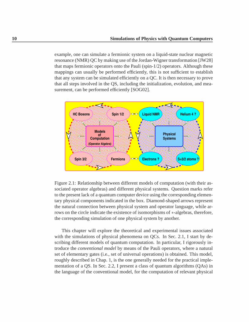
10 Simulations of Physics with Quantum Computers
example, one can simulate a fermionic system on a liquid-state nuclear magneticresonance (NMR) QC by making use of the Jordan-Wigner transformation [JW28]that maps fermionic operators onto the Pauli (spin-1/2) operators. Although thesemappings can usually be performed efficiently, this is not sufficient to establishthat any system can be simulated efficiently on a QC. It is thennecessary to provethat all steps involved in the QS, including the initialization, evolution, and mea-surement, can be performed efficiently [SOG02].
FermionsSpin 3/2
HC Bosons Spin 1/2
Modelsof
Computation
(Operator Algebra)
SystemsPhysical
Liquid NMR
S=3/2 atoms ?
Helium 4 ?
Electrons ?
Figure 2.1: Relationship between different models of computation (with their as-sociated operator algebras) and different physical systems. Question marks referto the present lack of a quantum computer device using the corresponding elemen-tary physical components indicated in the box. Diamond-shaped arrows representthe natural connection between physical system and operator language, while ar-rows on the circle indicate the existence of isomorphisms of∗-algebras, therefore,the corresponding simulation of one physical system by another.
This chapter will explore the theoretical and experimentalissues associatedwith the simulations of physical phenomena on QCs. In Sec. 2.1, I start by de-scribing different models of quantum computation. In particular, I rigorously in-troduce theconventional modelby means of the Pauli operators, where a naturalset of elementary gates (i.e., set of universal operations)is obtained. This model,roughly described in Chap. 1, is the one generally needed forthe practical imple-mentation of a QS. In Sec. 2.2, I present a class of quantum algorithms (QAs) inthe language of the conventional model, for the computationof relevant physical
2.1 Models of Quantum Computation 11
properties of quantum systems, such as correlation functions, energy spectra, etc.In Sec. 2.3, I explain how the QS of quantum physical systems obeying fermionic,anyonic, and bosonic particle statistics, can be performedon a QC described bythe conventional model, presenting some mappings between the different opera-tor algebras. As an application, in Sec. 2.4 I show the QS (imitated by a classicalcomputer) of a particular fermionic system: The two-dimensional fermionic Hub-bard model. It is expected that such simulation gives an insight into the limitationsof quantum computation, showing that certain issues remainto be solved to as-sure that a QC is more powerful than a CC (Sec. 2.5). In Sec. 2.7, I describethe experimental implementation on an NMR QC of the QS of another fermionicsystem: The Fano-Anderson model. For this purpose, an elementary introductionto the physical processes on an NMR setting is described in Sec. 2.6. Finally, Isummarize in Sec. 2.8.
2.1 Models of Quantum Computation
When performing a quantum computation, the quantum elements which constitutethe QC can be universally controlled and manipulated by modulating and chang-ing their interactions. This quantum control model assumesthen the existence ofa control HamiltonianHP , which describes these interactions. The control possi-bilities are used to implement specific quantum gates, allowing one, for example,to represent the time evolution of the physical system to be simulated [OGK01].
In order to define a model of quantum computation it is necessary to give aphysical setting together with its initial state, an algebra of operators associated tothe system, a set of controllable Hamiltonians necessary todefine a set of elemen-tary gates, and a set of measurable operators (i.e., observables). In this way, manydifferent models of quantum computation can be described, but for historic rea-sons and practical purposes I will focus mostly on theconventional model[NC00].
2.1.1 The Conventional Model of Quantum Computation
As mentioned in Chap. 1, in the conventional model of quantumcomputation, thefundamental unit of information is the quantum bit orqubit. A qubit’s pure state|a〉 = a|0〉 + b|1〉 (with a, b ∈ C and |a|2 + |b|2 = 1), is a linear superpositionof the logical states|0〉 and |1〉, and can be represented by the state of a two-level quantum system such as a spin-1/2. Assigned to each qubit are the identityoperator1l (i.e., the no-action operator) and the Pauli operatorsσx, σy, andσz. In

12 Simulations of Physics with Quantum Computers
the logical single-qubit basisB = |0〉, |1〉, these are
1l =
(1 00 1
), σx =
(0 11 0
), σy =
(0 −ii 0
), σz =
(1 00 −1
). (2.1)
Because of its action over the logical states, the operatorσx is usually referred astheflip operator:
σx
|0〉 → |1〉 ,|1〉 → |0〉 . (2.2)
For practical purposes in this thesis, it is also useful to define the raising (+) andlowering (-) Pauli operatorsσ± = 1
2(σx ± iσy), and the eigenstates of the flip
operator|+〉 = 1√2[|0〉+ |1〉] and|−〉 = 1√
2[|0〉 − |1〉], satisfying
σx|±〉 = ±|±〉. (2.3)
The Pauli operators form thesu(2) Lie algebra and satisfy the commutationrelations (µ, ν, λ = x, y, z)
[σµ, σν ] = i2ǫµνλσλ, (2.4)
where[A,B] = AB−BA andǫµνλ is the total anti-symmetric Levi-Civita symbol.They constitute a complete set of local observables, that is, a basis for the2 × 2dimensional Hermitian matrices withσµ = (σµ)
†. The symbol† denotes thecorresponding complex conjugate transpose.
Any qubit’s pure state can be represented as a point on the surface of theunit sphere (Bloch-sphere representation) by parametrizing the state as|a〉 =a|0〉+ b|1〉 = cos(θ/2)|0〉+ eiϕ sin(θ/2)|1〉 (Fig. 2.2). In order to process a singlequbit, a complete set of single-qubit gates has to be given. These operations con-stitute then, any rotation in the Bloch-sphere representation, which are given bythe operatorsRµ(ϑ) = e−i(ϑ/2)σµ = cos(ϑ/2)1l− i sin(ϑ/2)σµ; that is, a rotationby an angleϑ along theµ axis. These rotations are unitary (reversible) operations,satisfyingRµ(ϑ)[Rµ(ϑ)]
† = 1l (i.e., no-action), whereRµ(ϑ)† ≡ Rµ(−ϑ). This
reversibility property allows one to perform these gates with no thermodynami-cal cost. In Fig. 2.3, I present these elementary single-qubit gates in their circuitrepresentation.
Similarly, a pure state of aN-qubit register (quantum register) is representedas theket|ψ〉 =
∑2N−1n=0 an|n〉, where|n〉 is a product of states of each qubit in the
logical (or other) basis, e.g., its binary representation (|0〉 ≡ |0102 · · · 0N〉, |1〉 ≡|0102 · · · 0N−11N〉, |2〉 ≡ |0102 · · ·1N−10N〉, etc.), and
∑2N−1n=0 |an|2 = 1 (an ∈ C).

2.1 Models of Quantum Computation 13
x
z
y
θ
ϕ
j0i
j1i
jai
Figure 2.2: Bloch-Sphere representation of a one qubit state parametrized as|a〉 =cos(θ/2)|0〉 + eiϕ sin(θ/2)|1〉. The curved arrows denote rotationsRµ along thecorresponding axis. The (arrow) color convention is:|0〉 → blue;|1〉 → red; otherlinear combinations→magenta.
Assigned to thejth qubit of the quantum register are, together with the identityoperator1lj, the local Pauli operatorsσj
µ (with µ = x, y, or z); that is
σjµ =
n factors︷ ︸︸ ︷1l⊗ 1l⊗ · · · ⊗ σµ︸︷︷︸
jth factor
⊗ · · · ⊗ 1l ,
where⊗ represents a Kronecker tensorial product. Their matrix representation inthe basis ordered asB = |01 · · · 0N−10N〉, |01 · · · 0N−11N〉, · · · , |11 · · · 1N−11N〉is just the matrix tensor product of the corresponding2 × 2 matrices defined byEq. 2.1. For two different qubits, these operators commute:
[σjµ, σ
kν
]= 0 ∀j 6= k. (2.5)
In order to describe a generic operation on the quantum register, it is also nec-essary to consider products of the Pauli operatorsσj
µ. Remarkably, every uni-tary (reversible) operation acting on the quantum registercan be decomposedin terms of single qubit rotationsRj
µ(ϑ) = e−iϑ2σjµ and two-qubit gates, such
as the Ising gateRzjzk(ω) = e−iω2σjzσ
kz = cos(ω/2)1l − i sin(ω/2)σj
zσkz , with
ω ∈ R ([BBC95, DiV95]). The operationsRzjzk(ω) are also unitary, satisfy-ing Rzjzk(ω)[Rzjzk(ω)]
† = 1l, with [Rzjzk(ω)]† ≡ Rzjzk(−ω). Together with the
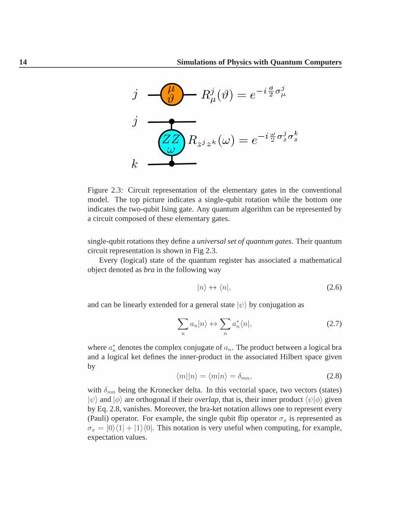
14 Simulations of Physics with Quantum Computers
Figure 2.3: Circuit representation of the elementary gatesin the conventionalmodel. The top picture indicates a single-qubit rotation while the bottom oneindicates the two-qubit Ising gate. Any quantum algorithm can be represented bya circuit composed of these elementary gates.
single-qubit rotations they define auniversal set of quantum gates. Their quantumcircuit representation is shown in Fig 2.3.
Every (logical) state of the quantum register has associated a mathematicalobject denoted asbra in the following way
|n〉 ↔ 〈n|, (2.6)
and can be linearly extended for a general state|ψ〉 by conjugation as
∑
n
an|n〉 ↔∑
n
a∗n〈n|, (2.7)
wherea∗n denotes the complex conjugate ofan. The product between a logical braand a logical ket defines the inner-product in the associatedHilbert space givenby
〈m||n〉 = 〈m|n〉 = δmn, (2.8)
with δmn being the Kronecker delta. In this vectorial space, two vectors (states)|ψ〉 and|φ〉 are orthogonal if theiroverlap, that is, their inner product〈ψ|φ〉 givenby Eq. 2.8, vanishes. Moreover, the bra-ket notation allowsone to represent every(Pauli) operator. For example, the single qubit flip operator σx is represented asσx = |0〉〈1|+ |1〉〈0|. This notation is very useful when computing, for example,expectation values.

2.1 Models of Quantum Computation 15
A measurementis defined as the action that gives some classical informationabout the state of the quantum register. In quantum mechanics, a measurementis considered to be a probabilistic process thatcollapsesthe actual quantum stateof the system [Per98]. For example, a measurement of the polarization in thelogical basis of every qubit (i.e., the measurement of the observablesσj
z) whenthe state of the register is|ψ〉 =
∑n an|n〉, projects it onto a certain logical state
|m〉 with probability |am|2 (Bohm’s rule). This is a von Neumann measurement.In particular, in a generalvon Neumannmeasurement of an observableM (≡M †), the probabilitypm that the outcomem is obtained, wherem is one possibleeigenvalue ofM , is given by [NC00]
pm = 〈ψ|M †mMm|ψ〉, (2.9)
whereMm is the projector onto the subspace of states with quantum numberm.Moreover, ifm is the actual outcome, the state after the measurement is given by
|ψ′〉 = Mm√〈ψ|M †
mMm|ψ〉|ψ〉. (2.10)
For example, when measuring the operatorσx for a single qubit state|0〉, thetwo possible outcomes arem = ±1 (i.e., the eigenvalues ofσx). Since|0〉 =1√2[|+〉+ |−〉], the corresponding probabilities are
p1 = p−1 = 1/2, (2.11)
and if the outcome is+1 (−1), the state is projected onto|+〉 (|−〉). Therefore,to obtain accurate information about the actual state of thequantum system, oneneeds to prepare many copies of the state and perform many different measure-ments.
The expectation value of a measurement outcome is the expectation of theoutcomes of many measurement repetitions. It can also be expressed in the bra-ket notation. If the state of the quantum system is|ψ〉, the expectation value ofMis given by
〈M〉 = 〈ψ|M |ψ〉. (2.12)
In the conventional model, any observableM can be written as a combination(sums and/or products) of the identity and Pauli operators.Therefore, if|ψ〉 isknown, the expectation〈M〉 can be algebraically computed by obtaining first thestateM |ψ〉, and by projecting it onto the bra〈ψ| using the inner-product relations

16 Simulations of Physics with Quantum Computers
of Eq. 2.8. For example, if a two-qubit state is given by|ψ〉 = 1√2[|0102〉+ |1112〉],
then
〈ψ|σ1z |ψ〉 =
1
2(〈0102|+ 〈1112|) (|0102〉 − |1112〉) = 0, (2.13)
and
〈ψ|σ1xσ
2x|ψ〉 =
1
2(〈0102|+ 〈1112|) (|1112〉+ |0102〉) = 1. (2.14)
Equations 2.13 and 2.14 have been obtained by noticing thatσ1z |1112〉 = −|1112〉,
σ1xσ
2x|0102〉 = |1112〉, andσ1
xσ2x|1112〉 = |0102〉, together with Eq. 2.8.
Nevertheless, certain quantum computations and QSs are done by evolvingmixed states instead of pure states. A quantum register in a probabilistic mixtureof pure states can be described in the bra-ket notation by a density matrixρ =∑
s psρs, with ρs = |ψs〉〈ψs| representing the quantum register being in the purestate|ψs〉, with probabilityps (
∑s ps = 1; ps ≥ 0). Equivalently, every density
operatorρ can also be written as a combination (sums and/or products) of thePauli operatorsσj
α (α = x, y, z) and the identity operator1l. These mixed statesare useful when performing quantum computation with devices such as the NMRQC, where the state of the quantum register is approximated by the average stateof an ensemble of molecules at room temperature; that is, an extremely mixedstate. The expectation value of a measurement outcome over amixed state isgiven by
〈M〉 = Tr(ρM), (2.15)
whereM is the measured observable,ρ the density operator of the mixed state,andTr denotes the trace.
In brief, the conventional model allows one to describe every step in a QS bymeans of Pauli operators. The idea is to represent any quantum algorithm (QA)as a circuit composed of elementary single and two-qubit gates, together with themeasurement process. The complexity of a QA is then determined by the amountof resources required, given by the number of qubits needed,the number of uni-versal single and two-qubit operations (Fig. 2.3), and the number of measurementsneeded to obtain an accurate result (e.g., the number of times that the algorithmneeds to be performed). For this purpose, a procedure to decompose an arbitraryoperation in terms of elementary gates has to be explained. In the following sub-section, I present some useful techniques and examples.

2.1 Models of Quantum Computation 17
2.1.2 Hamiltonian Evolutions
When simulating a physical system on a QC it is necessary, in general, to performa Hamiltonian (unitary) evolution to the quantum register [OGK01, SOG02], ofthe form
U(t) = e−iHt = 1l− iHt+ 1
2(−iHt)2 + · · · , (2.16)
whereH = H† is a physical Hamiltonian andt is a real parameter (e.g., time). AcommonH is given by
H = Hx +Hy = α σ1x
(j−1∏
i=2
σiz
)σjx + β σ1
y
(j−1∏
i=2
σiz
)σjy , (2.17)
whereα andβ are real numbers. From Eqs. 2.4 and 2.5 one obtains[Hx, Hy] = 0,and therefore,U(t) = e−iHxte−iHyt.
To decomposeU(t) into single and two-qubit operations, the following stepscan be taken. First, the unitary operator
U1 = eiπ4σ1y =
1√2
[1l + iσ1
y
](2.18)
takesσ1z → σ1
x, i.e.,U †1σ
1zU1 = σ1
x, soU †1e
iασ1zU1 = eiασ
1x. Second, the operator
U2 = eiπ4σ1zσ
2z =
1√2
[1l + iσ1
zσ2z
]
takesσ1x → σ1
yσ2z , soU †
2eiασ1
xU2 = eiασ1yσ
2z . Then,
U3 = eiπ4σ1zσ
3z
takesσ1yσ
2z → −σ1
xσ2zσ
3z . By successively similar steps the required string of
operators can be easily built:σ1xσ
2z · · ·σj−1
z σjx and alsoexp[iασ1
xσ2z · · ·σj−1
z σjx]
(up to a global irrelevant phase):
U †k · · ·U
†2U
†1e
iασ1zU1U2 · · ·Uk = exp
[iασ1
xσ2z · · ·σj−1
z σjx
](2.19)
where the integerk scales linearly withj. The evolutione−iHyt can be decom-posed similarly soU(t) is decomposed as the product of both decompositions.

18 Simulations of Physics with Quantum Computers
2.1.3 Controlled Operations
Alternatively, one can use the well known Controlled-Not, or CNOT, gate insteadof the two-qubit Ising gate. Its action on a pair of qubits (1 and 2) is
CNOT
|0102〉 → |0102〉 , |0112〉 → |0112〉 ,|1102〉 → |1112〉 , |1112〉 → |1102〉 .
Here, qubit 1 is the control qubit (the controlled operationon its state|11〉 is repre-sented by a solid circle in Fig. 2.4). If the state of qubit 1 is|01〉 nothing happens(identity operation) but if its state is|11〉, the state of qubit 2 is flipped. The de-composition of the CNOT unitary operation into single and two-qubit operationsis
CNOT: eiπ4 e−iπ
4σ1ze−iπ
4σ2xei
π4σ1zσ
2x , (2.20)
which was obtained by noticing thatie−iπ2σ2x ≡ σ2
x, i.e., the spin-flip operatoracting on qubit 2 (Eq. 2.1):
σ2x
|φ102〉 → |s112〉 ,|φ112〉 → |s102〉 .
(2.21)
By using the techniques described in Sec. 2.1.2, the CNOT operation in terms ofsingle and two-qubit Ising gates is
CNOT: eiπ4 e−iπ
4σ1ze−iπ
4σ2xei
π4σ2ye−iπ
4σ1zσ
2ze−iπ
4σ2y . (2.22)
The circuit representation of this decomposition is shown in Fig. 2.4. Five ele-mentary single and two-qubit Ising gates are required to perform the CNOT gate.
These results can be extended to other controlled unitary operations like theCU operation defined as
CU: |0〉a〈0| ⊗ 1ls + |1〉a〈1| ⊗ Us. (2.23)
The unitary operation above performs the transformationUs (also unitary) overa set of qubitss if the state of the control qubita is |1〉, and does not act other-wise. For the transformationUs ≡ U(t) = e−iQt, with Q = Q†, the operationalrepresentation of the CU gate is
U(t/2)U(t/2)−σaz , (2.24)
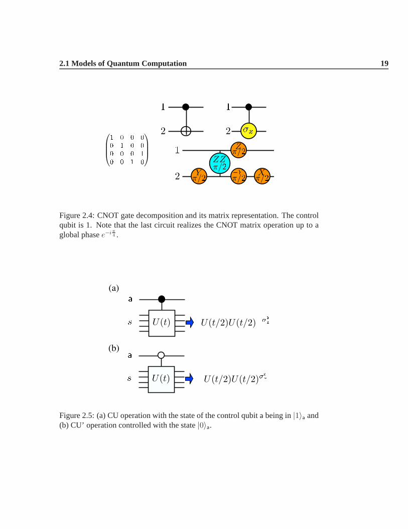
2.1 Models of Quantum Computation 19
Figure 2.4: CNOT gate decomposition and its matrix representation. The controlqubit is 1. Note that the last circuit realizes the CNOT matrix operation up to aglobal phasee−iπ
4 .
Figure 2.5: (a) CU operation with the state of the control qubit a being in|1〉a and(b) CU’ operation controlled with the state|0〉a.

20 Simulations of Physics with Quantum Computers
whereU(t/2)−σaz ≡ eiQ⊗σa
z [Fig. 2.5(a)]. Equivalently, one can define anothercontrolled operation, CU’, on the state|0〉a [Fig. 2.5(b)]:U(t/2)U(t/2)σ
az .
Controlled operations are widely used in quantum algorithms. In general, theirdecomposition into single and two-qubit gates require a large number of theseelementary operations, so they should be avoided when possible.
2.2 Deterministic Quantum Algorithms
In a QS, a QC performs certain tasks which are expected to givesome informationabout the physical system being simulated. These tasks are communicated bymeans of aprogram or quantum algorithm(QA), which can be schematicallyrepresented as a quantum circuit. In this section, I presenta particular type ofQA that can be used to obtain relevant properties of a quantumphysical systems,using the conventional model (Sec. 2.1). Nevertheless, thesame techniques canbe used to simulate physical systems with other particle statistics (e.g., fermionicor bosonic systems), if they can be described by Pauli operators after an algebraicmapping.
A deterministic QA is based on three different steps: i) the preparation of apure initial state, ii) its evolution, and iii) the measurement of certain property ofthe evolved state, in which the result of the algorithm is encoded. To preserve thefeatures of the quantum world, the evolution step is performed through a unitaryoperation and the measurement step is described by a certainobservable (i.e.,Hermitian operator). Here, I present only the class of QAs that allows one todetermine, in a register ofN qubits, physical correlation functions of the form
G = 〈φ|Ws|φ〉, (2.25)
whereWs is a unitary (reversible) operator associated to the systemto be simu-lated; that is,WsW
†s = 1l (s refers to the system).
Indirect measurement techniques can be used to obtain such correlation func-tions on a QC. In addition to the qubits used torepresentthe physical systemsto be simulated (i.e., the qubits-system) extra qubits, calledancillas, are required.These ancillas constitute the probes that contain information about the qubits-system. In the following section I describe different measurement techniques.
2.2 Deterministic Quantum Algorithms 21
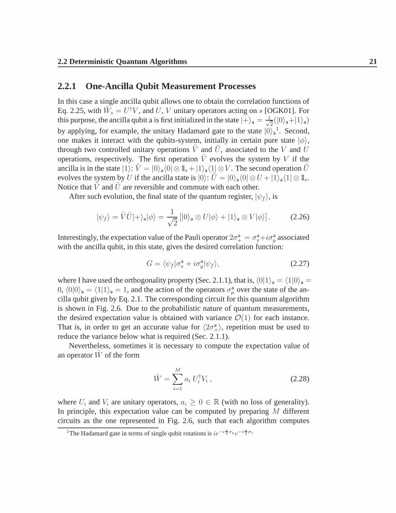
2.2.1 One-Ancilla Qubit Measurement Processes
In this case a single ancilla qubit allows one to obtain the correlation functions ofEq. 2.25, withWs = U †V , andU , V unitary operators acting ons [OGK01]. Forthis purpose, the ancilla qubita is first initialized in the state|+〉a = 1√
2(|0〉a+|1〉a)
by applying, for example, the unitary Hadamard gate to the state|0〉a1. Second,one makes it interact with the qubits-system, initially in certain pure state|φ〉,through two controlled unitary operationsV and U , associated to theV andUoperations, respectively. The first operationV evolves the system byV if theancilla is in the state|1〉: V = |0〉a〈0|⊗1ls+ |1〉a〈1|⊗V . The second operationUevolves the system byU if the ancilla state is|0〉: U = |0〉a〈0| ⊗U + |1〉a〈1| ⊗ 1ls.Notice thatV andU are reversible and commute with each other.
After such evolution, the final state of the quantum register, |ψf 〉, is
|ψf 〉 = V U |+〉a|φ〉 =1√2[|0〉a ⊗ U |φ〉+ |1〉a ⊗ V |φ〉] . (2.26)
Interestingly, the expectation value of the Pauli operator2σa+ = σa
x+iσay associated
with the ancilla qubit, in this state, gives the desired correlation function:
G = 〈ψf |σax + iσa
y|ψf 〉, (2.27)
where I have used the orthogonality property (Sec. 2.1.1), that is,〈0|1〉a = 〈1|0〉a =0, 〈0|0〉a = 〈1|1〉a = 1, and the action of the operatorsσa
µ over the state of the an-cilla qubit given by Eq. 2.1. The corresponding circuit for this quantum algorithmis shown in Fig. 2.6. Due to the probabilistic nature of quantum measurements,the desired expectation value is obtained with varianceO(1) for each instance.That is, in order to get an accurate value for〈2σa
+〉, repetition must be used toreduce the variance below what is required (Sec. 2.1.1).
Nevertheless, sometimes it is necessary to compute the expectation value ofan operatorW of the form
W =M∑
i=1
ai U†i Vi , (2.28)
whereUi andVi are unitary operators,ai ≥ 0 ∈ R (with no loss of generality).In principle, this expectation value can be computed by preparingM differentcircuits as the one represented in Fig. 2.6, such that each algorithm computes
1The Hadamard gate in terms of single qubit rotations isie−iπ4σye−iπ
2σz
22 Simulations of Physics with Quantum Computers
Figure 2.6: Quantum algorithm for the evaluation of the correlation G =〈φ|U †V |φ〉.
〈U †i Vi〉. However, in most practical cases, the preparation of the initial state|φ〉
is a very difficult task. This difficulty can then be reduced byusing a particularQA that requires only one circuit, but withL ancilla qubits, whereL = J +1 andJ ≥ log2M . Such QA has been described in Ref. [SOG02]. The idea is to extendthe results described above using controlled operations with respect to differentancilla qubits.
2.2.2 Quantum Algorithms and Quantum Simulations
Based on the indirect-measurement methods described in Sec. 2.2.1, I now presentcertain QAs for QSs. These are useful for obtaining relevantproperties of quan-tum systems, like the evaluation of the correlation function
G(t) = 〈φ|T †A†iTBj|φ〉. (2.29)
Here,Ai andBj are unitary operators (any operator can be decomposed in a uni-tary operator basis asA =
∑i
αiAi, B =∑j
βjBj), T = e−iHt is the time evo-
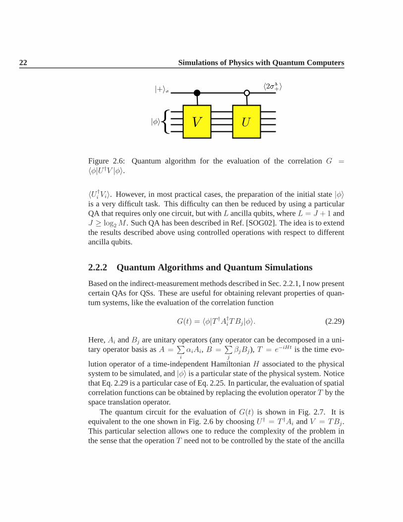
lution operator of a time-independent HamiltonianH associated to the physicalsystem to be simulated, and|φ〉 is a particular state of the physical system. Noticethat Eq. 2.29 is a particular case of Eq. 2.25. In particular,the evaluation of spatialcorrelation functions can be obtained by replacing the evolution operatorT by thespace translation operator.
The quantum circuit for the evaluation ofG(t) is shown in Fig. 2.7. It isequivalent to the one shown in Fig. 2.6 by choosingU † = T †Ai andV = TBj .This particular selection allows one to reduce the complexity of the problem inthe sense that the operationT need not to be controlled by the state of the ancilla
2.2 Deterministic Quantum Algorithms 23
Figure 2.7: Quantum algorithm for the computation of spatial and time-correlationfunctions. In this case,〈2σa
+〉 = 〈φ|T †A†iTBj|φ〉. Notice the simplification
achieved by reducing the controlled-T operations. The sameconvention ofFig. 2.6 has been used.
qubit ([SOG02]). As mentioned in Sec. 2.1.3, controlled operations require a largenumber of elementary gates, so they must be avoided when possible.
In brief, the computation ofG(t) is performed as follows: First, the ancillaqubit a is prepared in the state|+〉a, and the system is prepared in the state|φ〉.Second, a controlled evolution on the state|1〉a, given by C-B= |0〉a〈0| ⊗ 1ls +|1〉a〈1| ⊗ Bj , is performed. Third, the time evolutionT is performed. Fourth, acontrolled evolution on the state|0〉a, given by C-A= |0〉a〈0|⊗Ai+ |1〉a〈1|⊗1ls,is performed. Finally the observable〈2σa
+〉 = 〈σax + iσa
y〉 = G(t) is measured.
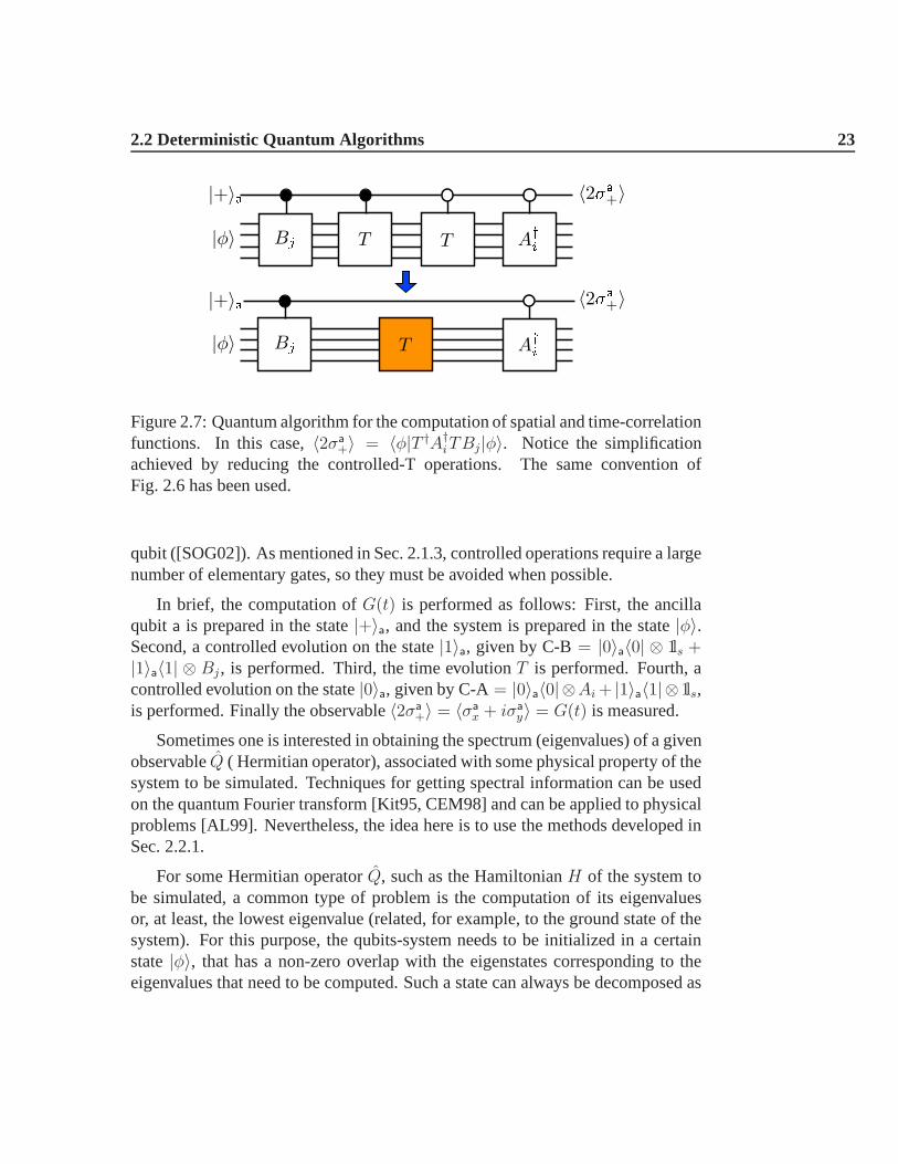
Sometimes one is interested in obtaining the spectrum (eigenvalues) of a givenobservableQ ( Hermitian operator), associated with some physical property of thesystem to be simulated. Techniques for getting spectral information can be usedon the quantum Fourier transform [Kit95, CEM98] and can be applied to physicalproblems [AL99]. Nevertheless, the idea here is to use the methods developed inSec. 2.2.1.
For some Hermitian operatorQ, such as the HamiltonianH of the system tobe simulated, a common type of problem is the computation of its eigenvaluesor, at least, the lowest eigenvalue (related, for example, to the ground state of thesystem). For this purpose, the qubits-system needs to be initialized in a certainstate|φ〉, that has a non-zero overlap with the eigenstates corresponding to theeigenvalues that need to be computed. Such a state can alwaysbe decomposed as
24 Simulations of Physics with Quantum Computers
9
>
>
>
>
>
>
=
>
>
>
>
>
>
;
e
i
^
Q
a
z
t
2
ji
h2
a
+
ia
j+i
Figure 2.8: Quantum algorithm for the computation of the spectrum of an observ-ableQ. In this case,〈2σa
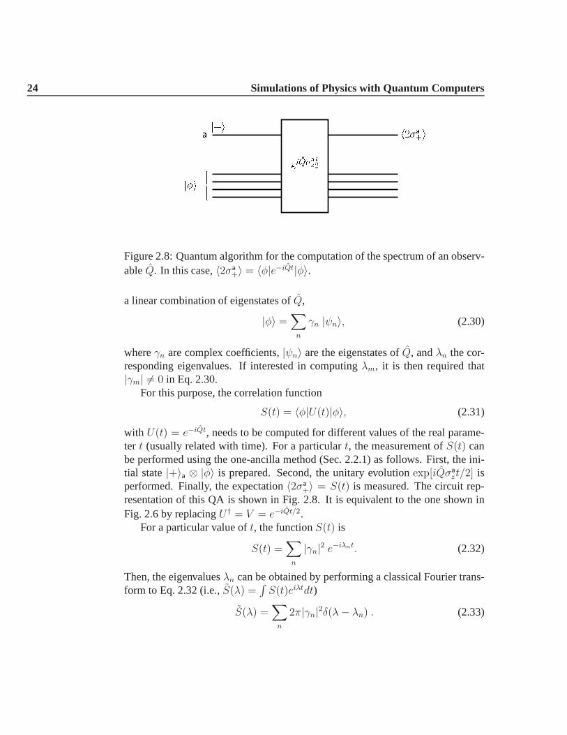
+〉 = 〈φ|e−iQt|φ〉.
a linear combination of eigenstates ofQ,
|φ〉 =∑
n
γn |ψn〉, (2.30)
whereγn are complex coefficients,|ψn〉 are the eigenstates ofQ, andλn the cor-responding eigenvalues. If interested in computingλm, it is then required that|γm| 6= 0 in Eq. 2.30.
For this purpose, the correlation function
S(t) = 〈φ|U(t)|φ〉, (2.31)
with U(t) = e−iQt, needs to be computed for different values of the real parame-ter t (usually related with time). For a particulart, the measurement ofS(t) canbe performed using the one-ancilla method (Sec. 2.2.1) as follows. First, the ini-tial state|+〉a ⊗ |φ〉 is prepared. Second, the unitary evolutionexp[iQσa
zt/2] isperformed. Finally, the expectation〈2σa
+〉 = S(t) is measured. The circuit rep-resentation of this QA is shown in Fig. 2.8. It is equivalent to the one shown inFig. 2.6 by replacingU † = V = e−iQt/2.
For a particular value oft, the functionS(t) is
S(t) =∑
n
|γn|2 e−iλnt. (2.32)
Then, the eigenvaluesλn can be obtained by performing a classical Fourier trans-form to Eq. 2.32 (i.e.,S(λ) =
∫S(t)eiλtdt)
S(λ) =∑
n
2π|γn|2δ(λ− λn) . (2.33)
2.3 Quantum Simulations of Quantum Physics 25
However,S(t) is only obtained for a discrete set of values oft. It is needed, in-stead, to calculate the corresponding discrete Fourier transform (see Appendix A)to obtain information about theλn’s.
2.3 Quantum Simulations of Quantum Physics
In the most general case, a QS requires the simulation of systems with diversedegrees of freedom, like fermions, anyons, bosons, etc. Theassociated Hilbertspaces (space of states) differ from the one defined for the conventional model.For example, in the case of fermionic systems, fermionic states are governed byPauli’s exclusion principle. Then, at most a single spinless (or two spin-1/2)fermion can occupy a certain (atomic) quantum state at the same time. There-fore, all the features associated with the physical system to be simulated must bepreserved when transforming its operators to the operatorsdescribing the compu-tational model of the QC.
In this section, I present isomorphic mappings that allow one to simulate ar-bitrary quantum systems, regardless of their particle statistics, by using the QAsdefined for the conventional model (Sec. 2.2). Fortunately,such mappings can beeasily performed without breaking the efficiency of a QA.
2.3.1 Simulations of Fermionic Systems
The systems considered here consist mainly of a lattice withN modes (sites),where spinless fermions can hop between sites. These results can be easily ex-tended for the case of spin-1/2 fermions or higher spin fermions.
In the second quantization representation, the (spinless)fermionic operatorsc†j andcj are defined as the creation and annihilation operators of a fermion in thej-th mode (j = 1, · · · , N), respectively. Due to the Pauli’s exclusion principle andthe antisymmetric nature of the fermionic wave function under the permutation oftwo fermions, the fermionic algebra is given by the following anticommutationrelations
ci, cj = 0, c†i , cj = δij (2.34)
where, denotes the anticommutator (i.e.,A,B = AB +BA).The Jordan-Wigner transformation [JW28] is the isomorphicmapping that al-
lows the description of a fermionic system by the conventional model. It is per-

26 Simulations of Physics with Quantum Computers
formed in the following way:
cj →(
j−1∏
l=1
−σlz
)σj−, (2.35)
c†j →(
j−1∏
l=1
−σlz
)σj+, (2.36)
where the Pauli operatorsσiµ were previously introduced in Sec 2.1. If these op-
erators satisfy thesu(2) commutation relations (Eqs. 2.4 and 2.5), the operatorsc†j andcj obey the anticommutation relations of Eqs. 2.34. This is an isomorphicmapping between operator algebras and is independent of theHamiltonian of thefermionic system to be simulated.
Different Hamiltonians establish different connections (connectivity) betweenfermionic modes. Historically, Eqs. 2.35 and 2.36 correspond to lattices in onespace dimension. Nevertheless, it is also valid for latticesystems in any dimen-sion, when the set of modesj is countable. In particular, the set of all orderedp-tuples of integers can be placed in one-to-one correspondence with the set ofintegers. For example, the simulation of a two dimensional fermionic lattice sys-tem can be done by re-mapping each mode(l, m) into a new set of modes asj = m+ (l − 1)Nx, where[l = 1 · · ·Ny] and[m = 1 · · ·Nx] are integer numbersthat refer to the position of a site in the lattice, andNx andNy are the number ofsites (modes) in thex andy direction, respectively.
In order to compute physical properties of a fermionic system on a QC de-scribed by the conventional model, every step of the quantumsimulation has tobe expressed in terms of Pauli operators. For a (spinless) fermionic system withN modes, a QC must contain, besides the ancilla qubita, N qubits to representthe system. In the following, I describe how certain fermionic initial states can beprepared and how they can be evolved under a particular fermionic Hamiltonianevolution.
Preparation of Initial Fermionic States
Associated to each fermionic mode, there are two levels which correspond to themode being empty or being occupied by a spinless fermion. Thestate-state map-ping is then trivial. Basically, the logical state|1j〉 is associated to thejth mode ifit is empty, and the logical state|0j〉 (up to a phase) is associated if thejth modeis occupied. In this way, the vacuum or no-fermion state|vac〉, which satisfiescj|vac〉 = 0 ∀j, is mapped to the logicalN-qubit state|1112 · · · 1N〉.
2.3 Quantum Simulations of Quantum Physics 27
However, when simulating a fermionic system, more complex states need tobe prepared. A general state|ψ〉 of Ne fermions is a linear combination of Slaterdeterminants (i.e., fermionic product states),
|ψ〉 =L∑
α=1
gα |φα〉, (2.37)
where the Slater determinants|φα〉 are
|φα〉 =Ne∏
j=1
c†j |vac〉. (2.38)
Due to the anticommutation relations of Eqs. 2.34, the fermionic operators satisfy
c†ic†j = −c†jc†i if i 6= j, (2.39)
implying that the Slater determinants|φα〉 are antisymmetric wave functions underthe permutation of an even number of fermions.
Every state|φα〉 can be prepared on a QC made of qubits, by noticing that thequantum gate (i.e., unitary operator)
Um = eiπ2(cm+c†m) (2.40)
creates a particle in them-th mode when acting on the vacuum state. In otherwords,Um|vac〉 = ei
π2 c†m|vac〉. Then, making use of the Jordan-Wigner transfor-
mation (Eqs. 2.35 and 2.36), the operatorsUm in the spin language are
Um = eiπ2σmx
m−1∏j=1
−σjz
. (2.41)
The operatorsUm can easily be decomposed into elementary single and two-qubitgates as described in Sec. 2.1.2. The successive application of Ne similar uni-tary operators to the state|1112 · · · 1N〉 generates the mapped state|φα〉, up to anirrelevant global phase.
The general fermionic state of Eq. 2.37 can be prepared by using L ancillaqubits, performing unitary controlled-Um evolutions on the state of the ancillas,and finally, performing a measurement (projecting) on the ancillas. For example,if one is interested in preparing the state|ψ〉 = 1√
2[|φ1〉 + |φ2〉], one needs to add
an extra ancilla to the system. This ancilla is prepared in the state|+〉a and a
28 Simulations of Physics with Quantum Computers
controlled evolution to obtain the state1√2[|0〉a⊗ |φ1〉+ |1〉a⊗ |φ2〉], is performed
later. If the Hadamard gate is applied to the ancilla, this state evolves into
|0〉a ⊗1√2[|φ1〉+ |φ2〉] + |1〉a ⊗
1√2[|φ1〉+ |φ2〉]. (2.42)
Therefore, the ancilla qubit is measured and projected, with probability 1/2, into|0〉a or |1〉a. If the former is obtained, the desired state is prepared. However, ifthe ancilla is projected into|1〉a, the whole method needs to be applied again fromthe begining.
In general, the probability of successful preparation of|ψ〉 (Eq. 2.37) usingthis method is1/L. Then, the order ofL trials need to be performed before asuccessful preparation. A detailed description of this method can be found inRef. [OGK01].
Nevertheless, an important case consists of the preparation of Slater determi-nants (product state)|φβ〉 in a different basis mode than the one given before:
|φβ〉 =Ne∏
j=1
d†j |vac〉. (2.43)
The fermionic operatorsd†j ’s are sometimes related to the operatorsc†j through thefollowing canonical transformation
−→d
†= eiM−→c †, (2.44)
with−→d
†= (d†1, d
†2, · · · , d†N), −→c † = (c†1, c
†2, · · · , c†N), and M being aN × N
Hermitian matrix. (Sometimes the operatorsd† are combinations of both, thecreation and annihilation operatorsc†i andci.)
Thouless’s theorem states that one Slater determinant evolves into the other as
|φβ〉 = U |φα〉, (2.45)
where the unitary fermionic operator
U = e−i−→c †
M,−→c (2.46)
can be written in terms of Pauli operators using the Jordan-Wigner transformation(Sec.2.3.1), and can also be decomposed into elementary gates as described inSec. 2.1.2.
2.3 Quantum Simulations of Quantum Physics 29
In brief, the described fermionic product states can be prepared on a QC de-scribed by the conventional model, if the Jordan-Wigner transformation is per-formed. Interestingly, the preparation can be done efficiently: the number of el-ementary single-qubit and two-qubit gates required scalespolynomially with thesystem sizeN . In Chap. 4, I present another class of fermionic states thatcan alsobe prepared efficiently.
Fermionic Evolutions
The evolution of a quantum state is the second step in the realization of a QA. Thegoal is to decompose a generic evolution into the elementarygatesRµ(ϑ) andRzjzk(ω)(Sec. 2.1). Sometimes, the evolution step is associated to aHermitian operatorHwhich is, for example, the HamiltonianH of the fermionic system to be simu-lated in terms of Pauli operators after Eqs. 2.35 and 2.36 have been performed. Inthis case, the corresponding evolution unitary operator isU(t) = e−iHt (i.e, thesolution to the Schrodinger’s evolution equation).
In general, a fermionic Hamiltonian can be decomposed asH = K+V ,whereK represents the kinetic energy of the fermions andV their potential energy. Usu-ally, [K, V ] 6= 0 and the decomposition ofU(t) in terms of elementary gates isa complicated task. To avoid this difficulty this operator isapproximated by, forexample, using a first order Trotter decomposition [Suz93].That is,
U(t) =
N∏
g=1
U(∆t), (2.47)
U(∆t) = eiH∆t = ei(K+V )∆t = eiK∆teiV∆t +O(∆t2), (2.48)
whereK andV are the termsK andV in Pauli operators, respectively. Therefore,for ∆t→ 0, U(∆t) ∼ eiK∆teiV∆t.
The potential energyV is usually a sum of commuting diagonal terms, andthe decomposition ofeiV∆t into elementary gates is simple. However, the kineticenergyK is usually a sum of noncommuting hopping terms of the formc†jck+c
†kcj
(bilinear fermionic operators), and its decomposition is again approximated. A
typical kinetic termei(c†jck+c†
kcj)∆t (j < k), when mapped onto the spin language
gives
e− i
2(σj
xσkx+σj
yσky )
k−1∏l=j+1
(−σlz)
= e− i
2σjxσ
kx
k−1∏l=j+1
(−σlz)
e− i
2σjyσ
ky
k−1∏l=j+1
(−σlz)
. (2.49)
30 Simulations of Physics with Quantum Computers
The decomposition of each term on the right hand side of Eq. 2.49 into elementarysingle and two-qubit gates was previously discussed in Sec.2.1.2. The amount ofelementary gates required depends on the distance|j−k|, and scales polynomiallywith that distance. Moreover, sinceH represents a physical system, it is a linearcombination of a polynomially large (withN) amount of fermionic operators.Then,U(t) can be performed efficiently by applying a polynomially large amount
of elementary gates. In the same way, the unitary operationU = e−i−→c †
M−→c of
Eq. 2.46 can also be efficiently implemented.Obviously, the accuracy of approximatingU(t) using the Trotter decomposi-
tion increases as∆t decreases. Then, a large amount of gates might be required toperform the desired evolution with small errors. To overcome this problem, onecould use a Trotter approximation of higher order in∆t [Suz93]. All these approx-imation methods do not destroy the efficiency of the QA. Moreover, the evolutionstep induced by fermionic physical Hamiltonians with higher order products ofcreation and annihilation operators can also be efficientlyimplemented using thesame techniques.
2.3.2 Simulations of Anyonic Systems
The concepts described in Sec. 2.3.1 can be extended to otherand more generalparticle statistics, namelyhard-coreanyons [BO01]. These are particles that alsoobey the Pauli’s exclusion principle: At most one (spinless) anyon can occupy asingle mode. Assigned to each mode of the lattice are the creation and annihilationanyonic operatorsa†j andaj , respectively. Their commutation relations are givenby (j ≤ j′)
[aj, aj′]θ = [a†j , a†j′]θ = 0 ,
[aj, a†j′]−θ = δjj′(1− (e−iθ + 1)nj′) , (2.50)
[nj, a†j′] = δjj′a
†j′ ,
wherenj′ = a†j′aj′ is the number operator,[A,B]θ = AB − eiθBA, andθ isthe statistical angle. In particular,θ = π mod(2π) represents canonical spinlessfermions, whileθ = 0 mod(2π) represents hard-core bosons.
In order to simulate this problem on a QC described by the conventionalmodel, the following isomorphic mapping between algebras can be performed:
a†j =∏
l<j
[e−iθ + 1
2+e−iθ − 1
2σlz
]σj+,

2.3 Quantum Simulations of Quantum Physics 31
aj =∏
l<j
[eiθ + 1
2+eiθ − 1
2σlz
]σj−, (2.51)
nj =1
2(1 + σj
z),
where the Pauli operatorsσiµ were introduced in Sec. 2.1.1. Since they satisfy
the commutation relations of Eqs. 2.4 and 2.5, the commutation relations for theanyonic operators (Eqs. 2.50) are satisfied.
As in the fermionic case (Sec. 2.3.1), an anyonic evolution operator can bewritten in terms of Pauli operators using Eq. 2.51, and can bedecomposed intosingle and two-qubit elementary gates. Therefore, the sameprocedure describedin the previous section can be followed.
Anyon statistics have fermion and hard-core boson statistics as limiting cases,satisfying always the Pauli’s exclusion principle. In the next section this hard-corecondition is relaxed and the important case of canonical bosons is considered.
2.3.3 Simulations of Bosonic Systems
Quantum computation is based on the manipulation of quantumsystems that pos-sess a finite number of degrees of freedom (e.g., qubits). From this point ofview, the simulation of bosonic systems appears to be impossible, since the non-existence of an exclusion principle implies that the Hilbert space used to representbosonic quantum states on a lattice is infinite-dimensional; that is, there is no limitto the number of bosons that can occupy a given modej. However, sometimesit is necessary to simulate and study properties such that the use of the completeHilbert space is unnecessary, and only a finite sub-basis of states is sufficient. Thisis the case forN-mode (e.g.,N sites) lattice systems with interactions given bythe boson-preserving Hamiltonian
H =N∑
j,j′=1
αjj′ b†jbj′ + βjj′ njnj′, (2.52)
where the operatorsb†j (bj) create (destroy) a boson at sitej, andnj = b†jbj is thenumber operator; that is
b†j |n1, n2, · · · , nj , · · · , nN〉 =√nj + 1 |n1, n2, · · · , nj + 1, · · · , nN 〉,
bj |n1, n2, · · · , nj , · · · , nN〉 =√nj |n1, n2, · · · , nj − 1, · · · , nN〉,
nj |n1, n2, · · · , nj , · · · , nN〉 = nj |n1, n2, · · · , nj, · · · , nN〉, (2.53)
32 Simulations of Physics with Quantum Computers
where the bosonic state|n1, n2, · · · , nj , · · · , nN〉 represents a quantum state withnj bosons in thej-th mode (site).
The space dimension of the lattice is encoded in the parametersαjj′ andβjj′of the Hamiltonian. SinceH contains pairs of creation and annihilation operators,the total number of bosonsNP in the system is preserved and the idea is to work inthis finite sub-basis of states (where the dimension of the associated Hilbert spacedepends on the magnitude ofNP ).
The corresponding bosonic commutation relations (in an infinite-dimensionalHilbert space) are [CDG98]
[bj , bj′] = 0, [bj, b†j′] = δjj′. (2.54)
However, if the operatorsb†j are restricted to the finite basis of states representedby |n1, n2, · · · , nN〉 with max(ni) = NP, that is,NP is the maximum numberof bosons per site, they acquire the following matrix representation (see Eqs. 2.53)
b†j = 1l⊗ · · · ⊗ 1l⊗ b†︸︷︷︸jth factor
⊗1l⊗ · · · ⊗ 1l (2.55)
where the symbol⊗ indicates the usual tensorial product between matrices, andthe(NP + 1)× (NP + 1) dimensional matrices1l andb† are given by
1l =
1 0 0 · · · 00 1 0 · · · 00 0 1 · · · 0...
...... · · · ...
0 0 0 · · · 1
, b† =
0 0 0 · · · 0 01 0 0 · · · 0 00√2 0 · · · 0 0
......
... · · · ......
0 0 0 · · ·√NP 0
. (2.56)
It is important to note that in this finite basis, the commutation relations of theb†idiffer from the standard bosonic ones (Eq. 2.54) [BO02]
[bi, bj] = 0, [bi, b†j] = δij
[1− NP + 1
NP !(b†i )
NP (bi)NP
], (2.57)
and clearly(b†j)NP+1 = 0.
Since the goal is to simulate the bosonic system on a QC described by the con-ventional model, a corresponding mapping between both operator algebras mustbe given. Nevertheless, Eqs. 2.57 imply that the linear spanof the operatorsb†j andbj is not closed under the commutator, and a mapping between thebosonic oper-ators and the Pauli operators like the Jordan-Wigner transformation (Sec. 2.3.1)

2.3 Quantum Simulations of Quantum Physics 33
is not possible. Therefore, such isomorphic mapping needs to be found by firstmapping quantum bosonic states onto quantum logical statesin the conventionalmodel (i.e., a Hilbert space mapping).
The idea is to start by considering only thejth mode in the chain. Sincethis mode can be occupied with at mostNP bosons, it is possible to associate an(NP +1)-qubit quantum state to each particle number state, in the following way:
|0〉j ↔ |001112 · · · 1NP〉j
|1〉j ↔ |100112 · · · 1NP〉j
|2〉j ↔ |101102 · · · 1NP〉j (2.58)
......
|NP 〉j ↔ |101112 · · · 0NP〉j
where|n〉j denotes a quantum state withn bosons injth mode. Therefore,N(NP+1) qubits for the simulation (whereN is the total number of modes) are needed.An example of this mapping for a quantum state with 7 bosons ina chain of 5sites, where the maximum number of bosons per site isNP = 3, is shown inFig. 2.9.
By definition (see Eqs. 2.53, 2.55, and 2.56)b†j |n〉j =√n+ 1 |n+ 1〉j, and
this operator in the conventional model maps to
b†j → b†j =NP−1∑
n=0
√n+ 1 σn,j
− σn+1,j+ , (2.59)
where a pair(n, j) refers to thenth qubit in the chain of qubits representing thejth bosonic mode. The Pauli creation and annihilation operatorsσk
± were previ-ously defined in Sec. 2.1. The operatorb†j acts then on the(NP + 1)-qubit chainrepresenting thejth bosonic mode as
b†j |10 · · ·1n−10n1n+1 · · ·1NP〉j =
√n+ 1 |10 · · ·1n0n+11n+2 · · ·1NP
〉j , (2.60)
so its matrix representation in this basis is analogous to the matrix representationof b†j in the basis of bosonic states.
Similarly, the number operator is mapped as
nj → nj =
NP∑
n=0
nσn,jz + 1
2, (2.61)

34 Simulations of Physics with Quantum Computers
5
4
3
2
i = 1
n = 0 1 2 3
j
i =
1
2
p
3
b
y
1
(b
y
2
)
3
b
y
3
(b
y
4
)
2
jva i
j
i = j#"##i
1
j###"i
2
j#"##i
3
j##"#i
4
j"###i
5
Figure 2.9: Mapping of the bosonic state|φα〉, of a chain with 5 sites and 7 bosons(NP = 3), into a four-spin-1/2 (or four-qubit) state. The convention is|↑j〉 ≡ |0j〉and|↓j〉 ≡ |1j〉.
so its action over the corresponding logical states is
nj|10 · · · 1n−10n1n+1 · · · 1NP〉j = n |10 · · · 1n0n+11n+2 · · · 1NP
〉j. (2.62)
Since the commutator[b†j ,∑NP
n=0 σn,jz ] = 0 the operatorsb†j (bj) always keep states
within the same subspace.
The Hamiltonian of Eq. 2.52 in terms of Pauli operators is then
H =N∑
j,j′=1
αjj′ b†j bj′ + βjj′ njnj′, (2.63)
where the operatorsb†j (bj) are given by Eqs. 2.59, andnj by Eq. 2.61. In thisway, physical properties of the bosonic system such as the spectrum ofH canbe obtained using a QC made of qubits. The same methods can be used whensimulating any other type of boson-preserving quantum system.

2.3 Quantum Simulations of Quantum Physics 35
Preparation of Initial Bosonic States
As in the fermionic case, the most general bosonic state of anN-mode lattice sys-tem with a maximum ofNP bosons per site can be written as a linear combinationof bosonic product states like
|φα〉 = K(b†1)n1(b†2)
n2 · · · (b†N)nN |vac〉, (2.64)
whereK is a normalization factor,nj is the number of bosons at sitej (max(nj) =NP ), and|vac〉 is vacuum or no-boson state, that is,bj |vac〉 = 0 ∀j.
Using the mapping described in Eq. 2.58, the vacuum state in the conventionalmodel maps as
|vac〉 → |0011 · · · 1NP〉1 ⊗ · · · ⊗ |0011 · · · 1NP
〉N , (2.65)
and the product state of Eq. 2.64 maps as
|φα〉 = |10 · · · 0n1 · · · 1NP〉1 ⊗ · · · ⊗ |10 · · · 0nN
· · · 1NP〉N (2.66)
(see Fig. 2.9 for an example).The preparation of the mapped bosonic state|φα〉 on a QC made of qubits
is then performed by flipping the states of the correspondingqubits from a fullypolarized state (i.e., the logical state with all qubits in|1〉), using for example theflip operationsσn,j
x . Nevertheless, more general bosonic states like
|ψ〉 =L∑
α=1
gα |φα〉 (2.67)
can also be realized as in the fermionic case. Again, the ideais to addL ancillas(extra qubits), perform controlled evolutions on their states, and finally performmeasurements on the state of the ancillas. The state is successfully prepared withprobability1/L [OGK01].
Bosonic Evolutions
Again, the idea is to represent certain bosonic unitary evolution operatorU(t) =e−iHt, whereH is some boson-preserving Hermitian operator such as the Hamilto-nian of the system to be simulated (Eq. 2.52), in terms of Pauli operators (Eq. 2.63).Usually, a first order Trotter approximation [Suz93] also needs to be performed toseparate those terms inH that do not commute.

36 Simulations of Physics with Quantum Computers
In general,H = K+V (Eq. 2.52), whereK is a kinetic term andV a potentialterm. The kinetic term is a linear combination of terms likeb†kbl+b
†l bk. Therefore,
a single-step evolution operatorei(b†kbl+b†
lbk)∆t is mapped onto Pauli operators as
exp
[iϑ
NP−1∑
n,n′=0
√(n + 1)(n′ + 1) [(σn,k
x σn+1,kx + σn,k
y σn+1,ky )(σn′,l
x σn′+1,lx +
σn′,ly σn′+1,l
y ) + (σn,kx σn+1,k
y − σn,ky σn+1,k
x )(σn′,lx σn′+1,l
y − σn′,ly σn′+1,l
x )]],(2.68)
whereϑ = ∆t/8 andNP is the maximal number of bosons per site. The termsin the exponent of Eq. 2.68 commute with each other, so the decomposition intoelementary gates can be done using the methods described in Sec. 2.1.2. As anexample, consider a system of two sites with maximal one boson per site (NP =1). Thus,2(1 + 1) = 4 qubits are needed for the simulation, and Eq. 2.59 impliesthat b†1 = σ0,1
− σ1,1+ andb†2 = σ0,2
− σ1,2+ . The mapped bosonic operatorei(b
†1b2+b†2b1)∆t
in terms of Pauli operators is
exp(iϑσ0,1x σ1,1
x σ0,2x σ1,2
x )× exp(iϑσ0,1x σ1,1
x σ0,2y σ1,2
y )× (2.69)
exp(iϑσ0,1y σ1,1
y σ0,2x σ1,2
x )× exp(iϑσ0,1y σ1,1
y σ0,2y σ1,2
y )× exp(iϑσ0,1y σ1,1
x σ0,2y σ1,2
x )×exp(−iϑσ0,1
y σ1,1x σ0,2
x σ1,2y )× exp(−iϑσ0,1
x σ1,1y σ0,2
y σ1,2x )× exp(iϑσ0,1
x σ1,1y σ0,2
x σ1,2y ),
and the decomposition of each of the terms in Eq. 2.69 in termsof single andtwo-qubit elementary gates can be done, again, using the methods described inSec. 2.1.2. An example of the decomposition of the termexp
(it8σ0,1x σ1,1
y σ0,2y σ1,2
x t),
where the qubits were relabeled as(n, j) ≡ n+2j− 1 (e.g.,(0, 1)→ 1) is shownin Fig. 2.10.
Contrary to the fermionic case, the number of elementary operations involvedin the decomposition is not related to the distance between sites,|k− l|. Neverthe-less, a physical bosonic operatorH, such as the Hamiltonian of Eq. 2.52, involvesa polynomially large number (with respect toN) of bosonic terms. Therefore, thecorresponding evolutionU(t) = e−iHt can be efficiently performed on a QC byapplying a polynomially large number of elementary single and two-qubit gates.Again, when using approximate methods like the Trotter decomposition, the num-ber of operations needed increases with the desired accuracy. However, such anapproximation does not destroy the efficiency of the simulation.

2.4 Applications: The 2D fermionic Hubbard model 37
1
2
3
4
1
2
3
4
e
i
8
1
x
2
y
3
y
4
x
t
e
i
4
3
x
e
i
4
4
y
e
i
4
1
z
4
z
e
i
4
2
z
3
z
e
i
4
2
y
e
i
4
1
x
e
i
8
1
z
2
z
t
e
i
4
2
y
e
i
4
1
x
e
i
4
2
z
3
z
e
i
4
1
z
4
z
e
i
4
4
y
e
i
4
3
x
t
Figure 2.10: Decomposition of the unitary operatorU(t) = eit8σ1xσ
2yσ
3yσ
4x into ele-
mentary gates as described in Sec. 2.1.2. The labeling convention is (0, 1) ≡ 1,(1, 1) ≡ 2, (0, 2) ≡ 3, and(1, 2) ≡ 4.
2.4 Applications: The 2D fermionic Hubbard model
To clarify the methods described previously, in this section I present, as an ex-ample, the QS of the finite two-dimensional fermionic Hubbard model by usinga CC that imitates a QC; that is, aquantum simulator. Since this is a classicalsimulation, the CC must keep track of an exponentially largenumber of quantumstates, associated with the Hilbert space of the quantum system. Nevertheless, thissimulation provides a good example for understanding the advantages and resultsthat can be obtained when using a real QC.
The physical system to be simulated consists of a rectangular lattice (Fig. 2.11),with Nx ×Ny sites, where spin-1/2 fermions hop from site to site under the inter-action Hamiltonian
H = −∑
(i,j);σ
[txc†(i,j);σc(i+1,j);σ + tyc
†(i,j);σc(i,j+1);σ +H.C.] + U
∑
(i,j)
n(i,j);↑n(i,j);↓ ,
(2.70)where the operatorsc†(i,j);σ (c(i,j);σ) create (annihilate) a fermion with spin compo-nent denoted byσ (=↑ or ↓), at the site located at(x = i, y = j). tx andty are the

38 Simulations of Physics with Quantum Computers
t
x
t
y
U
bond#m
(N
x
; 1)(1; 1)
(N
x
; N
y
)
(i; j)
Figure 2.11: Two-dimensional lattice in the Hubbard model.
hopping terms in thex andy directions, respectively, andn(i,j);σ = c†(i,j);σc(i,j);σis the corresponding number operator. (H.C. denotes the Hermitian conjugate).Periodic boundary conditions (PBC) are assumed:[(i, j); σ] ≡= [(i+Nx, j); σ] ≡[(i, j +Ny); σ].
To use the QA for the obtention of the spectrum ofH, described in Sec. 2.2.2,it is necessary first to map the fermionic operators onto Pauli operators using, forexample, the Jordan-Wigner transformation (Sec. 2.3.1). Considering that theseare spin-1/2 fermions, the QA needs2(Nx × Ny) qubits to represent the system(qubits system), plus the ancilla qubit.
Assuming that one is mainly interested in obtaining the lowest energy ofEq. 2.70, the prepared initial state should be the ground state of Eq. 2.70. How-ever, since no algebraic methods exist to exactly diagonalize Eq. 2.70 for largeNx
andNy, such a state is not known, and therefore impossible to prepare. Neverthe-less, the ground state of the associated mean-field Hamiltonian
HMF = −∑
(i,j);σ
[txc†(i,j);σc(i+1,j);σ + tyc
†(i,j);σc(i,j+1);σ +H.C.] +
U∑
(i,j)
[〈n(i,j);↑〉n(i,j);↓ + n(i,j);↑〈n(i,j);↓〉 − 〈n(i,j);↑〉〈n(i,j);↓〉] , (2.71)
is known to be a fermionic product state (Slater determinant) |φβ〉, and its corre-

2.5 Quantum Algorithms: Efficiency and Errors 39
sponding state in the conventional model can be efficiently prepared by using themethods described in Sec. 2.3.1; that is, it can be prepared by applying a polyno-mially large (with respect toNx×Ny) set of elementary gates to the fully polarizedstate. For finite small lattices,|φβ〉 is a good approximation to the ground state ofEq. 2.70 and can be used to obtain the ground state energy.
The second step of the QA is to apply the unitary operatorU(t) = eiHσazt/2
using single and two-qubit gates (see Fig. 2.8 forQ ≡ H)), where, in this case,H is the Hamiltonian of Eq. 2.70 in terms of Pauli operators,t is a real (fixed)parameter, andσa
z is the Pauli operator associated with the ancilla qubit. SinceHis a linear combination of non-commuting terms (Eq. 2.70), the operatorU(t) =∏
j U(∆t) can be approximated by using, for example, the first order Trotter de-composition [Suz93]. That is,H = K↑ +K↓ + V , whereKσ denotes the kineticenergy associated with the fermions of spinσ andV denotes the potential energy.Then,
U(∆t) = e−iHσaz∆t/2 ∼ e−iK↑σ
az∆t/2 × e−iK↓σ
az∆t/2 × e−iV σa
z∆t/2, (2.72)
whereKσ andV are the corresponding terms in Pauli operators. Also, the sameapproximation can be used to decompose each terme−iKσσa
z∆t/2. Such approxi-mation leads to operators that can easily be decomposed in terms of elementarygates by using the methods described in Sec. 2.1.2.
The energy spectrum of the Hubbard model for a4 × 2 lattice is shown inFig. 2.12. It has been obtained after running the classical simulation for manydifferent values oft, and performing the Fourier transform on the data. The peaksshow the eigenvalues and the results are compared to those ofan exact diagonal-ization method.
The algorithm described allows one to easily obtain the energy spectra of afinite small lattice. Nevertheless, the spectra of a large lattice cannot be efficientlyobtained using the same methods. The problem is that the ground state of themean-field approximation differs more from the ground stateof Eq. 2.70 as thesystem increases, and the QA needs to be performed an exponentially large num-ber of times (with respect toNx ×Ny) to obtain the desired property [SOG02].
2.5 Quantum Algorithms: Efficiency and Errors
A QA for a physical simulation is considered efficient if the total number of opera-tions involved for the initial state preparation, the evolution, and the measurement

40 Simulations of Physics with Quantum Computers
-10.50 -10.25 -10.00 -9.75 -9.50 -9.25 -9.00
0
2000
4000
6000
8000
10000
12000
14000
-8.0 -7.5 -7.0 -6.5 -6.0
0
500
1000
1500
2000
2500
Energy
-9.8278
-10.2469(-9.832899)
(-10.252953)
Energy
(-7.546672)-7.5428
j
~
F j
Figure 2.12: Energy spectrum of the Hubbard model obtained simulating the QAof Fig. 2.8 on a CC. The lattice has4×2 sites (which requires 16+1 qubits). Here,tx = ty = 1, andU = 4. The time steps used in the Trotter approximation to pre-pare the initial state and apply the evolution are∆t1 = ∆t2 = 0.05, respectively.The numbers in brackets are the results obtained from the exact diagonalizationusing the Lanczos method.

2.5 Quantum Algorithms: Efficiency and Errors 41
process, scales at most polynomially with the system size and with 1/ǫ, whereǫis the maximal tolerable error in the measurement of a relevant property.
While the decomposition of the operatorU(t) = e−iHt can be done efficiently(e.g., when using the Trotter approximation) ifH is a physical operator, the prepa-ration of a general initial state could be inefficient. Such inefficiency would arise,for example, if the state|ψ〉 defined in Eq. 2.37 or Eq. 2.67 is a linear combina-tion of an exponentially large number of elementary productstates. In this case,L ∼ xN , with N the number of modes in the system andx > 1, so an exponen-tially large number of trials need to be performed before successful preparation.However, ifL ≤ poly(N), it can be prepared efficiently. This construction gen-eralizes to more general coherent states (see Chap. 4).
The three main reasons for the existence of errorsǫ in the outcome of thequantum computation are gate imperfections, the use of the Trotter approxima-tion in the evolution operator, and the statistics in measuring the polarizationof the ancilla qubit (Sec. 2.2.2). Gate imperfections are very common in quan-tum information because, contrary to classical information, quantum gates areusually dominated by a continuous parameter. This problem can be solved byusing quantum error correction methods and fault tolerant quantum computa-tion [Ste96, Kit97, NC00, Got97]. According to the accuracythreshold theorem,provided that the physical gates have sufficiently low error, it is possible to quan-tum compute accurately in an efficient way.
The type of error introduced by the discretization of the evolution operatorU(t) (e.g., by using the Trotter decomposition or other approximations) is verysimilar to the error obtained when performing a classical simulation, such as whenusing Monte Carlo methods. This error can be estimated by a detailed analysis ofthe discretization and can also be arbitrarily reduced in anefficient way.
Finally, when using the QAs described in Sec. 2.2.2, the stepcorrespondingto the measurement process can also be performed efficientlybecause it only in-volves the measurement of a single (ancilla) qubit, regardless of the number ofqubits needed for the simulation. Nevertheless, repeatedly many same-simulationsneed to be performed to get an accurate value of such measurement. This is an in-herent property of the quantum mechanichs where a single measurement projectsthe quantum state (Sec. 2.1.1) and does not give sufficient information. If the rel-evant signal at the end of the quantum computation is small, like when obtainingthe spectra of the two-dimensional Hubbard model on a large lattice (Sec. 2.4), itis necessary to run the algorithm a larger number of times andthe efficiency canbe destroyed.
In brief, a QC can only be more efficient than a CC when simulating quan-
42 Simulations of Physics with Quantum Computers
tum physical systems if the three main steps of the corresponding QA can beperformed efficiently. For example, the evaluation of certain correlation functionsover a quantum state that can be easily prepared, can be efficiently done with aQC. In general (i.e., for non-integrable Hamiltonians), there is no known way toevaluate such correlation efficiently with a CC [SOG02, SOK03].
2.6 Experimental Implementations of Quantum Al-gorithms
In this chapter, I have shown that if a large QC existed today,some simulationsof quantum systems could be performed more efficiently on it than on a CC. Nev-ertheless, I did not discuss how the corresponding QAs couldbe experimentallyimplemented. Although numerous proposals for implementing quantum informa-tion processors (QIPs) are found in the literature [CZ95, CLK00, KLM01], onlyfew of them have been successfully implemented to process more than one qubit.In particular, liquid-state NMR devices allow one to simulate several systems bymanipulating, nowadays, up to ten qubits [RBC04].
The physical implementation of a large scale QC still remains one of the mostimportant challenges for today’s physicists. The problem is a QC should be de-signed such that the interaction between its constituents and the environment issmall enough to keep coherence of the quantum state. But if such interaction istoo small, the manipulation and control processes using external sources becomesimpracticable. For this reason, quantum decoherence has been one of the mostimportant subjects of study during the last decade. In general, decoherence phe-nomena is hard to predict due to the infinite degrees of freedom associated withthe environment. Nevertheless, a QC is reliable whenever the time required toperform a certain task is much smaller than the corresponding decoherence time.
In this section, I describe the experimental setting of a liquid-state NMR QIPand show how such devices can be used to execute the QAs described previously.Later on, I will show the experimental NMR simulation of a particular fermionicsystem, where some correlation functions and energy spectra have been obtained.
2.6.1 Liquid-State NMR Quantum Information Processor
Liquid-state NMR methods allow one to physically implementa slightly differentversion of the conventional model of quantum computation, with respect to the

2.6 Experimental Implementations of Quantum Algorithms 43
initial state preparation and the measurement process. In this set-up the quantumregister is represented by the average state of the nuclear spin-1/2 of an ensembleof identical molecules. Each nuclear spin is a two-level physical system and canthen be considered a possible qubit. Thus, the idea is to perform single and two-qubit elementary gates by external radio-frequency (rf) pulses that interact withthe nuclear spin state. In the following, I present a basic analysis about how theseprocessors can be used as possible QCs.
In a liquid NMR setting, the molecules are placed in a strong magnetic fieldB(z) ≃ 10 T, so that the spin of thej-th nucleus of a single molecule precessesat its Larmor frequencyνj (Fig. 2.13). In the frame rotating with thejth spin, itsqubit state can then be rotated by sending rf pulses in the XY plane at the resonantfrequencyνr ≈ νj . If the duration of this pulse isδt, the corresponding evolutionoperator in the rotating frame is [LKC02]
Uj = e−iHjδt = e−iA(cos(ϕ)σjx+sin(ϕ)σj
y)δt, (2.73)
whereA is the amplitude of the RF-pulse andϕ is its phase (i.e., orientation) inthe XY plane (~ = 1). Then, one can induce single spin rotations2 around anyaxis in that plane by adjustingδt andϕ.
Single-qubit rotations around thez axis can be implemented with no exper-imental imperfection or physical duration simply by changing the phase of theabstract rotating frame with which one is working. One has then to keep track ofall these phase changes with respect to a reference phase associated with the spec-trometer. Nevertheless, these phase tracking calculations are linear with respectto the number of pulses and spins, and can be efficiently done on a classical com-puter. Together with the rotations around any axis in the XY plane, thez rotationscan generate any single qubit rotation on the Bloch sphere.
Two-qubit gates, like the Ising gateRzjzk(ω) (Sec. 2.1.1), can be performedby taking advantage of the spin-spin interactions (i.e., nuclei interaction) presentin the molecule, and then achieve universal control. To firstorder in perturbation,this interaction, named theJ-coupling, has the form
Hj,k =Jjk4σjzσ
kz , (2.74)
wherej, k denote the corresponding pair of qubits andJjk is their coupling strength.Under typical NMR operating conditions, these interactionterms are small enough
2One actually is restricted to 90 and 180 degrees rotations for experimental calibration issues.

44 Simulations of Physics with Quantum Computers
Figure 2.13: Bloch’s sphere representation of a single nuclear spin-1/2 state pre-cessing around the quantization axis determined by the external magnetic fieldB.The precession frequency is given byνj = µjB, with µj the magnetic momentof thejth nucleus. Due to the chemical environment, each nucleus precesses at adifferent Larmor frequencyνj.
to be neglected when performing single-qubit rotations with rf pulses of short du-ration. Nevertheless, between two pulses they are driving the evolution of thesystem. By cleverly designing a pulse sequence, i.e., a succession of pulses andfree evolution periods, one can easily apply two-qubit gates on the state of thesystem. Indeed, the so-calledrefocusing techniques’ principleconsists of per-forming an arbitrary Ising gate by flipping one of the coupledspins (π-pulse),as shown in Fig 2.14. The interaction evolutions before and after the refocusingpulse compensate, leading to the effective evolution
U effj,k = ei
π2σjxe−i
Jjk4
σjzσ
kz δt2e−iσj
xπ/2e−iJjk4
σjzσ
kz δt1 = e−i α
4σjzσ
kz , (2.75)
where the effective coupling strengthα = Jjk(δt1 − δt2) is being determined bythe difference between the durationsδt1 andδt2.
Although the physics on a single molecule has been analyzed,liquid-stateNMR uses an ensemble of about1023 molecules in a solution maintained at roomtemperature (≃ 300K). For typical values of the magnetic field, this thermal stateis extremely mixed. Clearly, this is not the usual state in which one initializesa quantum computation since qubits are nearly randomly mixed. Nevertheless,
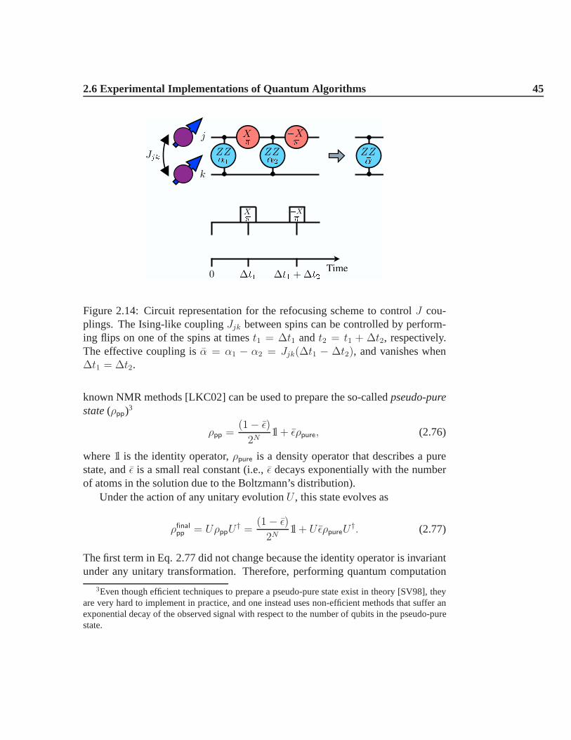
2.6 Experimental Implementations of Quantum Algorithms 45
Figure 2.14: Circuit representation for the refocusing scheme to controlJ cou-plings. The Ising-like couplingJjk between spins can be controlled by perform-ing flips on one of the spins at timest1 = ∆t1 andt2 = t1 + ∆t2, respectively.The effective coupling isα = α1 − α2 = Jjk(∆t1 − ∆t2), and vanishes when∆t1 = ∆t2.
known NMR methods [LKC02] can be used to prepare the so-called pseudo-purestate(ρpp)3
ρpp =(1− ǫ)2N
1l + ǫρpure, (2.76)
where1l is the identity operator,ρpure is a density operator that describes a purestate, andǫ is a small real constant (i.e.,ǫ decays exponentially with the numberof atoms in the solution due to the Boltzmann’s distribution).
Under the action of any unitary evolutionU , this state evolves as
ρfinalpp = UρppU† =
(1− ǫ)2N
1l + UǫρpureU†. (2.77)
The first term in Eq. 2.77 did not change because the identity operator is invariantunder any unitary transformation. Therefore, performing quantum computation
3Even though efficient techniques to prepare a pseudo-pure state exist in theory [SV98], theyare very hard to implement in practice, and one instead uses non-efficient methods that suffer anexponential decay of the observed signal with respect to thenumber of qubits in the pseudo-purestate.

46 Simulations of Physics with Quantum Computers
on the ensemble is equivalent to performing quantum computation over the initialstate represented only byρpure.
At the end of the computation, the orthogonal components of the sample po-larization in the XY plane,Mx = Tr(ρfinalpp
∑Ni=1 σ
ix), andMy = Tr(ρfinalpp
∑Ni=1 σ
iy)
are measured (Eq. 2.15). Note that the invariant component of ρfinalpp does not con-tribute to the signal sinceTr(1lσj
x,y) = 0. Because the polarization of each singlespin,M j
x = Tr(ρfinalpp σjx) andM j
y = Tr(ρfinalpp σjy), precesses at its own Larmor fre-
quencyνj, a Fourier transformation of the temporal recording (called FID, forFree Induction Decay) of the total magnetization needs to beperformed. By do-ing so, one obtains the expectation value of the polarization of each spin (averagedover all molecules in the sample).
Summarizing, a liquid-state NMR setting allows one to initialize a register ofqubits in a pseudo-pure state, apply any unitary transformation to this state bysending controlled rf pulses or by leaving free interactionperiods, and measurethe expectation value of some quantum observables (i.e., the spin polarization).Hence, these systems can be used as QIPs.
2.7 Applications: The Fano-Anderson Model
I now present the experimental QS of the fermionic one-dimensional (1D) Fano-Anderson model using a liquid-state NMR [NSO05], by manipulating the state ofthe spin nuclei as described in Sec. 2.6.1. Such simulation shows then how reliablethese experimental methods are and how well the elementary gates (Sec. 2.1.1) canbe implemented using NMR techniques.
The 1D fermionic Fano-Anderson model consists of ann-sites ring with an im-purity in the center (Fig. 2.15), where spinless fermions can hop between nearest-neighbors sites with hopping matrix element (overlap integral) τ , or between a siteand the impurity with matrix elementV/
√n. Taking the single-particle energy of
a fermion in the impurity to beǫ, and considering the translational invariance ofthe system, the Fano-Anderson Hamiltonian can be written inthe wave vectorrepresentation as [OGK01]
H =n−1∑
l=0
εklc†klckl + ǫb†b+ V (c†k0b+ b†ck0), (2.78)
where the fermionic operatorsc†kl and b† (ckl and b) create (destroy) a spinlessfermion in the conduction modekl and in the impurity, respectively. Here, the
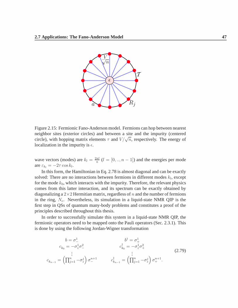
2.7 Applications: The Fano-Anderson Model 47
Rj
T
a
V√n
ǫ
Figure 2.15: Fermionic Fano-Anderson model. Fermions can hop between nearestneighbor sites (exterior circles) and between a site and theimpurity (centeredcircle), with hopping matrix elementsτ andV/
√n, respectively. The energy of
localization in the impurity isǫ.
wave vectors (modes) arekl = 2πln
(l = [0, .., n − 1]) and the energies per modeareεkl = −2τ cos kl.
In this form, the Hamiltonian in Eq. 2.78 is almost diagonal and can be exactlysolved: There are no interactions between fermions in different modeskl, exceptfor the modek0, which interacts with the impurity. Therefore, the relevant physicscomes from this latter interaction, and its spectrum can be exactly obtained bydiagonalizing a2×2Hermitian matrix, regardless ofn and the number of fermionsin the ring,Ne. Nevertheless, its simulation in a liquid-state NMR QIP is thefirst step in QSs of quantum many-body problems and constitutes a proof of theprinciples described throughout this thesis.
In order to successfully simulate this system in a liquid-state NMR QIP, thefermionic operators need to be mapped onto the Pauli operators (Sec. 2.3.1). Thisis done by using the following Jordan-Wigner transformation
b = σ1− b† = σ1
+
ck0 = −σ1zσ
2− c†k0 = −σ1
zσ2+
......
ckn−1=(∏n
j=1−σjz
)σn+1− c†kn−1
=(∏n
j=1−σjz
)σn+1+ .
(2.79)

48 Simulations of Physics with Quantum Computers
b
y
y
k
0
y
k
2
jva i $ j"
1
"
2
#
3
"
4
#
5
i $ j0
1
0
2
1
3
0
4
1
5
i
1
2
3
4
5
impurity
k
0
k
1
k
2
k
3
Figure 2.16: Mapping of the fermionic product stateb†c†k0c†k2|vac〉 into a five-qubit
state, using the Jordan-Wigner transformation. The convention is |↑j〉 ≡ |0j〉(filled) and|↓j〉 ≡ |1j〉 (empty).
In this language, a logical state|0j〉 (with |0〉 ≡ |↑〉 in the usual spin-1/2 notation)corresponds to having a spinless fermion in either the impurity, if j = 1, or in themodekj−2, otherwise (Fig. 2.16). (Again, the fermionic vacuum state|vac〉 mapsonto|vac〉 = |1112 · · · 1n+1〉.)
The algorithms described in Sec. 2.2.2 can be used, for example, to evaluatethe probability amplitude of having a fermion in modek0 at time t, if initially(t = 0) the quantum state is the Fermi sea state withNe fermions; that is,|FS〉 =Ne−1∏l=0
c†kl|vac〉. This probability is given by the modulus square of the following
dynamical correlation function:
G(t) = 〈FS|b(t)b†(0)|FS〉 , (2.80)
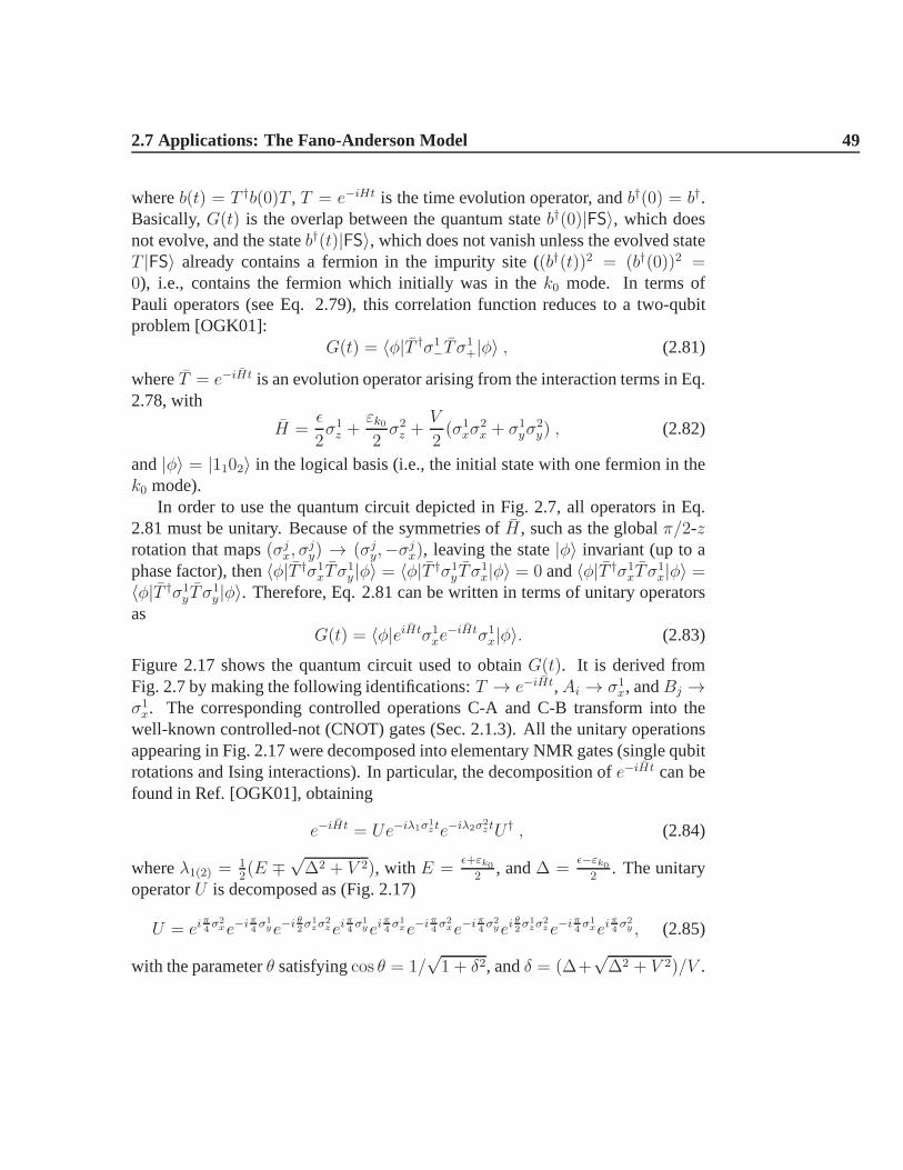
2.7 Applications: The Fano-Anderson Model 49
whereb(t) = T †b(0)T , T = e−iHt is the time evolution operator, andb†(0) = b†.Basically,G(t) is the overlap between the quantum stateb†(0)|FS〉, which doesnot evolve, and the stateb†(t)|FS〉, which does not vanish unless the evolved stateT |FS〉 already contains a fermion in the impurity site ((b†(t))2 = (b†(0))2 =0), i.e., contains the fermion which initially was in thek0 mode. In terms ofPauli operators (see Eq. 2.79), this correlation function reduces to a two-qubitproblem [OGK01]:
G(t) = 〈φ|T †σ1−T σ
1+|φ〉 , (2.81)
whereT = e−iHt is an evolution operator arising from the interaction termsin Eq.2.78, with
H =ǫ
2σ1z +
εk02σ2z +
V
2(σ1
xσ2x + σ1
yσ2y) , (2.82)
and|φ〉 = |1102〉 in the logical basis (i.e., the initial state with one fermion in thek0 mode).
In order to use the quantum circuit depicted in Fig. 2.7, all operators in Eq.2.81 must be unitary. Because of the symmetries ofH, such as the globalπ/2-zrotation that maps(σj
x, σjy) → (σj
y,−σjx), leaving the state|φ〉 invariant (up to a
phase factor), then〈φ|T †σ1xT σ
1y |φ〉 = 〈φ|T †σ1
yT σ1x|φ〉 = 0 and〈φ|T †σ1
xT σ1x|φ〉 =
〈φ|T †σ1yT σ
1y|φ〉. Therefore, Eq. 2.81 can be written in terms of unitary operators
asG(t) = 〈φ|eiHtσ1
xe−iHtσ1
x|φ〉. (2.83)
Figure 2.17 shows the quantum circuit used to obtainG(t). It is derived fromFig. 2.7 by making the following identifications:T → e−iHt,Ai → σ1
x, andBj →σ1x. The corresponding controlled operations C-A and C-B transform into the
well-known controlled-not (CNOT) gates (Sec. 2.1.3). All the unitary operationsappearing in Fig. 2.17 were decomposed into elementary NMR gates (single qubitrotations and Ising interactions). In particular, the decomposition ofe−iHt can befound in Ref. [OGK01], obtaining
e−iHt = Ue−iλ1σ1zte−iλ2σ2
ztU † , (2.84)
whereλ1(2) = 12(E ∓
√∆2 + V 2), with E =
ǫ+εk02
, and∆ =ǫ−εk0
2. The unitary
operatorU is decomposed as (Fig. 2.17)
U = eiπ4σ2xe−iπ
4σ1ye−i θ
2σ1zσ
2zei
π4σ1yei
π4σ1xe−iπ
4σ2xe−iπ
4σ2yei
θ2σ1zσ
2ze−iπ
4σ1xei
π4σ2y , (2.85)
with the parameterθ satisfyingcos θ = 1/√1 + δ2, andδ = (∆+
√∆2 + V 2)/V .
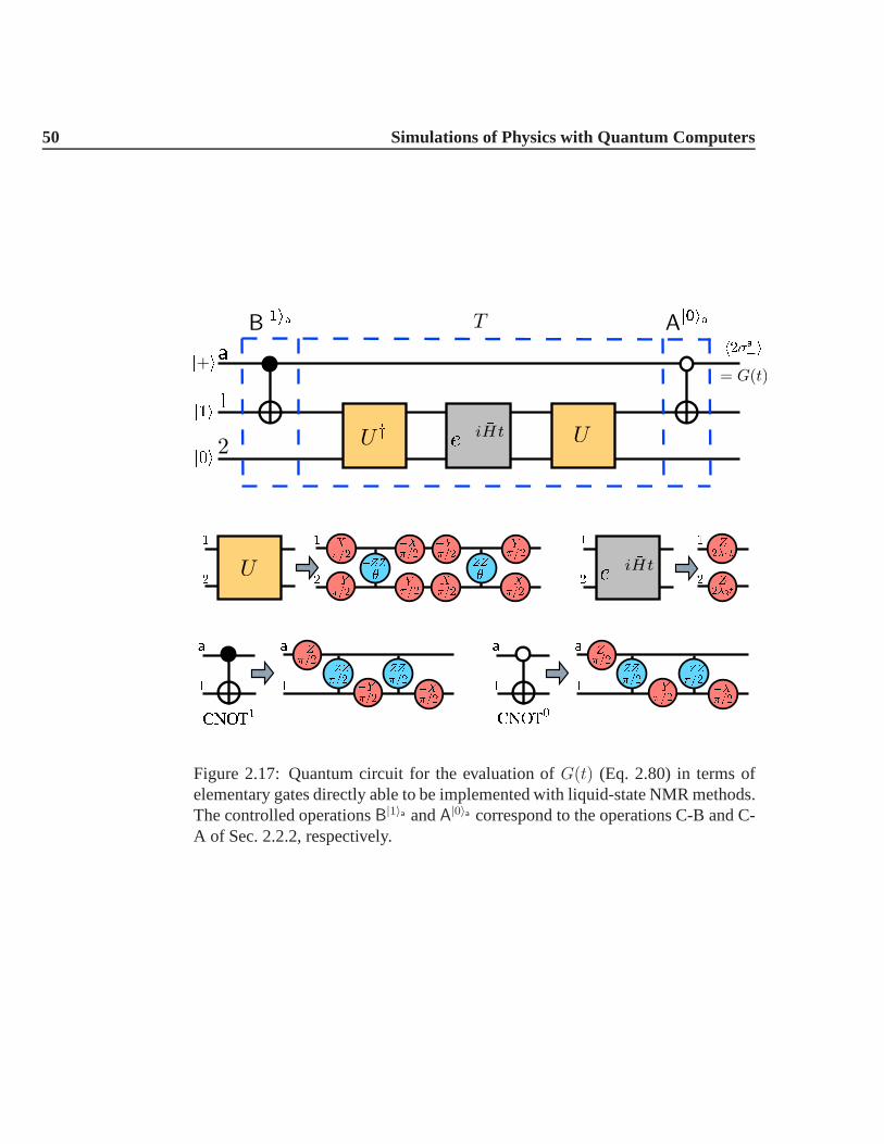
50 Simulations of Physics with Quantum Computers
Figure 2.17: Quantum circuit for the evaluation ofG(t) (Eq. 2.80) in terms ofelementary gates directly able to be implemented with liquid-state NMR methods.The controlled operationsB|1〉a andA|0〉a correspond to the operations C-B and C-A of Sec. 2.2.2, respectively.

2.7 Applications: The Fano-Anderson Model 51
The CNOT gates C-A and C-B can also be decomposed into elementary gates,as explained in Sec. 2.1.2. Therefore,G(t) can be obtained using an NMR QIP byapplying the appropriate rf pulses (Sec. 2.6.1). Remarkably, only three qubits arerequired for the simulation (Fig. 2.17): The ancilla qubita, one qubit representingthe impurity site (qubit-1), and one qubit representing thek0 mode (qubit-2).
Similarly, the algorithm depicted in Fig. 2.8 can be used if interested in ob-taining the spectrum of the HamiltonianH of Eq. 2.78, replacingQ → H. Inparticular, whenn = 1 (one site plus the impurity), Eq. 2.78 in terms of Paulioperators reduces toH =
ǫ+εk02
+ H, with H defined in Eq. 2.82. In this case, thetwo eigenvaluesλi (i = 1, 2) of the one-particle subspace can be extracted fromthe correlation function
S(t) = 〈φ|e−iHt|φ〉 = e−i(ǫ+εk0)t〈φ|e−iHt|φ〉, (2.86)
which can be obtained by measuring the polarization of the ancilla qubit after thequantum circuit shown in Fig. 2.8 has been applied. Since|φ〉 = |1102〉 is not aneigenstate ofH, it has a non-zero overlap with the two one-particle eigenstates,called|1Pi〉 (see Appendix B).
Again, the operatoreiHσazt/2 (Fig. 2.8) needs to be decomposed into elementary
gates for its implementation in an NMR QIP. Noticing that[σaz , H] = [σa
z , U ] = 0,then
eiHσazt/2 = Ueiλ1σ1
zσazt/2eiλ2σ2
zσazt/2U †ei(ǫ+εk0)σ
azt/2, (2.87)
where the unitary operatorU is decomposed as in Eq. 2.85. Figure 2.18 shows thecorresponding circuit in terms of elementary gates. Again,qubits 1 and 2 representthe impurity site and thek0 mode, respectively.a denotes the ancilla qubit. Sincethe idea is to perform a DFT on the results obtained from the measurement (seeAppendix B), this circuit needs to be applied for several values of the parametert(Sec. 2.1.3).
2.7.1 Experimental Protocol and Results
The NMR setting used for the evaluation ofG(t) andS(t) is based on an ensem-ble solution of trans-crotonic acid and methanol dissolvedin acetone (Fig. 2.19).This molecule can be used as a seven-qubit register, where methanol is used toperform rf-power selection and accurately calibrate the rfpulses. In this way, thedecoherence time (T ∗
2 ) is in the range from several hundreds of milliseconds tomore than a second, allowing one to perform around 1000 single-qubit gates andaround 100 two-qubit (Ising) gates.
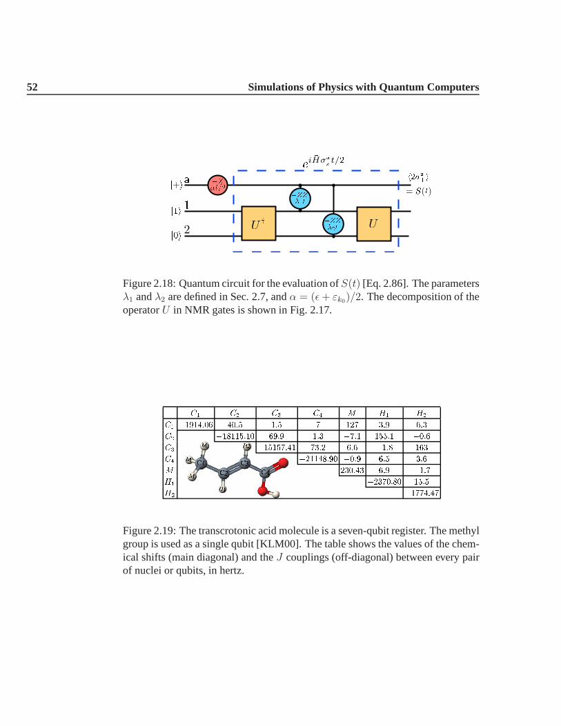
52 Simulations of Physics with Quantum Computers
Figure 2.18: Quantum circuit for the evaluation ofS(t) [Eq. 2.86]. The parametersλ1 andλ2 are defined in Sec. 2.7, andα = (ǫ+ εk0)/2. The decomposition of theoperatorU in NMR gates is shown in Fig. 2.17.
C
1
C
2
C
3
C
4
M H
1
H
2
C
1
1914:06 40:5 1:5 7 127 3:9 6:3
C
2
18115:10 69:9 1:3 7:1 155:1 0:6
C
3
15157:41 73:2 6:6 1:8 163
C
4
21148:90 0:9 6:5 3:6
M 230:43 6:9 1:7
H
1
2370:80 15:5
H
2
1774:47
Figure 2.19: The transcrotonic acid molecule is a seven-qubit register. The methylgroup is used as a single qubit [KLM00]. The table shows the values of the chem-ical shifts (main diagonal) and theJ couplings (off-diagonal) between every pairof nuclei or qubits, in hertz.
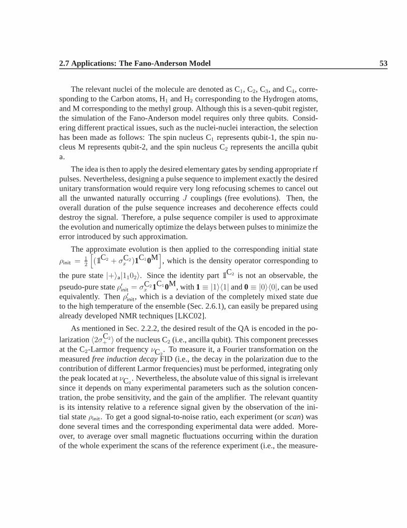
2.7 Applications: The Fano-Anderson Model 53
The relevant nuclei of the molecule are denoted as C1, C2, C3, and C4, corre-sponding to the Carbon atoms, H1 and H2 corresponding to the Hydrogen atoms,and M corresponding to the methyl group. Although this is a seven-qubit register,the simulation of the Fano-Anderson model requires only three qubits. Consid-ering different practical issues, such as the nuclei-nuclei interaction, the selectionhas been made as follows: The spin nucleus C1 represents qubit-1, the spin nu-cleus M represents qubit-2, and the spin nucleus C2 represents the ancilla qubita.
The idea is then to apply the desired elementary gates by sending appropriate rfpulses. Nevertheless, designing a pulse sequence to implement exactly the desiredunitary transformation would require very long refocusingschemes to cancel outall the unwanted naturally occurringJ couplings (free evolutions). Then, theoverall duration of the pulse sequence increases and decoherence effects coulddestroy the signal. Therefore, a pulse sequence compiler isused to approximatethe evolution and numerically optimize the delays between pulses to minimize theerror introduced by such approximation.
The approximate evolution is then applied to the corresponding initial state
ρinit = 12
[(1lC2 + σC2
x )1C10M], which is the density operator corresponding to
the pure state|+〉a|1102〉. Since the identity part1lC2 is not an observable, the
pseudo-pure stateρ′init = σC2x 1C10M, with 1≡ |1〉〈1| and0≡ |0〉〈0|, can be used
equivalently. Thenρ′init, which is a deviation of the completely mixed state dueto the high temperature of the ensemble (Sec. 2.6.1), can easily be prepared usingalready developed NMR techniques [LKC02].
As mentioned in Sec. 2.2.2, the desired result of the QA is encoded in the po-
larization〈2σC2+ 〉 of the nucleus C2 (i.e., ancilla qubit). This component precesses
at the C2-Larmor frequencyνC2. To measure it, a Fourier transformation on the
measuredfree induction decayFID (i.e., the decay in the polarization due to thecontribution of different Larmor frequencies) must be performed, integrating onlythe peak located atνC2
. Nevertheless, the absolute value of this signal is irrelevantsince it depends on many experimental parameters such as thesolution concen-tration, the probe sensitivity, and the gain of the amplifier. The relevant quantityis its intensity relative to a reference signal given by the observation of the ini-tial stateρinit. To get a good signal-to-noise ratio, each experiment (orscan) wasdone several times and the corresponding experimental datawere added. More-over, to average over small magnetic fluctuations occurringwithin the durationof the whole experiment the scans of the reference experiment (i.e., the measure-
54 Simulations of Physics with Quantum Computers
ment of the reference signal) are interlaced with scans of the actual complete pulsesequence. To increase the spatial homogeneity of the field over the sample, sev-eral automated shimming periods, consisting of fine tuning small additional coilslocated around the sample, have been inserted.
In Fig. 2.20, I show the experimental results obtained for the evaluation ofG(t) for εk0 = −2, ǫ = −8, V = 4, and εk0 = −2, ǫ = 0, V = 4, and fordifferent values oft. The duration of the optimized pulse sequences from thebeginning of the initialization step to the beginning of thedata acquisition, was97 ms. For comparison, the analytical form ofG(t), as well as the simulateddata points (i.e., data points obtained by simulating the quantum algorithm on aconventional computer) are also shown in the figure.
In Fig. 2.21, I present the experimental results obtained for the evaluationof S(t), to obtain the corresponding eigenvalues for the Hamiltonian, withεk0 =−2, ǫ = −8, andV = 0.5. The pulse sequence applied is the one corresponding tothe quantum circuit shown in Fig. 2.18 with the corresponding refocusing pulses.In Fig. 2.21, I also show the analytical and simulated data points. The DFT ofthe experimental data is shown in Fig. 2.22, revealing the expected peaks at thefrequency corresponding to the two one-particle eigenvalues of Eq. 2.78, for theabove parameters.
The close agreement between the experimental results and the correspondingsimulations, using the refocusing pulses, suggests that the main contribution toerrors comes from the incomplete refocusing scheme used in the optimizationprocedure. Therefore, increasing the number of refocusingpulses might have ledto more accurate results even if they would have increased the overall duration ofthe pulse sequence.
2.8 Summary
Throughout this chapter, I have addressed several broad issues associated with thesimulation of physical phenomena with QCs. In particular, Ipresented efficientways to map the algebras of operators associated to the physical system to besimulated onto the algebra of Pauli operators. These mappings are sufficient toestablish the equivalence of the different physical modelsto a universal model ofquantum computation: The conventional model.
I also explored various issues associated with simulations(Sec. 2.3), remark-ing that every step in a QA must be performed efficiently to have an efficientsimulation. Although a QC can simulate some quantum physical systems more

2.8 Summary 55
0 1 2 3-1
-0.5
0
0.5
1
Re[
G(t
)]
0 1 2 3-1
-0.5
0
0.5
1
Im[G
(t)]
0 1 2 3-1
-0.5
0
0.5
1
Re[
G(t
)]
0 1 2 3Time (s)
-1
-0.5
0
0.5
1
Im[G
(t)]
Figure 2.20: Real and imaginary parts of the correlation functionG(t) of Eq. 2.80.The top panels show the results when the parameters in Eq. 2.78 areεk0 = −2, ǫ =−8, V = 4. The corresponding parametersλ1, λ2, θ can be determined using Eqs.2.84 and 2.85. The bottom panels show the results forεk0 = −2, ǫ = 0, V = 4.The (black) solid line is the analytic solution, the red circles are obtained by thenumerical simulation (including the refocusing pulses), and the blue circles withthe error bars are experimental data.

56 Simulations of Physics with Quantum Computers
0 2 4 6 8 10 12
0.6
0.8
1
1.2
Re[
S(t
)]
0 2 4 6 8 10 12Time(s)
-0.4
-0.2
0
0.2
0.4
Im[S
(t)]
Figure 2.21: Real and imaginary parts ofS(t), for εk0 = −2, ǫ = −8, andV = 0.5 in Eq. 2.78. The (black) solid line corresponds to the analytic solution.The red circles correspond to the numerical simulation (using refocusing pulses)and the blue circles with the error bars are experimental data. S(t) has beenmeasured using the network of Fig. 2.18 withα = (ǫ+ εk0)/2.

2.8 Summary 57
−30 −20 −10 0 10 20 30
0
0.2
0.4
0.6
0.8
1
(freq.)
j
~
S()j
= 0
(
2
= 0)
= 9:87
(
1
= 10)
Figure 2.22: Discrete Fourier transform of the real part of the experimental dataof Fig. 2.21. The position of the two peaks corresponds to thetwo eigenvalues ofthe Hamiltonian of Eq. 2.78 forεk0 = −2, ǫ = −8, andV = 0.5. Numbers inparentheses denote the exact solution. The size of the dots representing experi-mental points is the error bar (see Appendix B). An upper bound to the error inthe frequency domain is≈ 0.5, which was determined by the resolution of thespectrum due to the time sampling of the simulation.
58 Simulations of Physics with Quantum Computers
efficiently than its classical analogue, I showed that many challenges still remainto prove this statement in a general way (Sec. 2.5). As an example, I presented theQS of the two-dimensional fermionic Hubbard model, where there is no knownway to obtain its ground state energy efficiently using a QC.
Finally, I described the experimental implementation of a QA using a liquid-state NMR QIP (Sec. 2.7). This experiment allows one to understand the advan-tages and disadvantages of simulating physical systems with today’s QCs, and, inparticular, to understand the power of quantum computation.
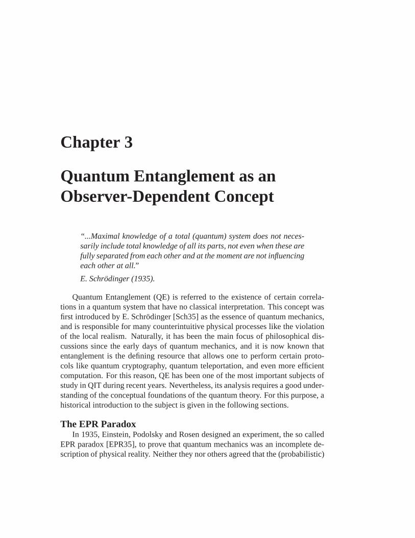
Chapter 3
Quantum Entanglement as anObserver-Dependent Concept
“...Maximal knowledge of a total (quantum) system does not neces-sarily include total knowledge of all its parts, not even when these arefully separated from each other and at the moment are not influencingeach other at all.”
E. Schrodinger (1935).
Quantum Entanglement (QE) is referred to the existence of certain correla-tions in a quantum system that have no classical interpretation. This concept wasfirst introduced by E. Schrodinger [Sch35] as the essence ofquantum mechanics,and is responsible for many counterintuitive physical processes like the violationof the local realism. Naturally, it has been the main focus ofphilosophical dis-cussions since the early days of quantum mechanics, and it isnow known thatentanglement is the defining resource that allows one to perform certain proto-cols like quantum cryptography, quantum teleportation, and even more efficientcomputation. For this reason, QE has been one of the most important subjects ofstudy in QIT during recent years. Nevertheless, its analysis requires a good under-standing of the conceptual foundations of the quantum theory. For this purpose, ahistorical introduction to the subject is given in the following sections.
The EPR ParadoxIn 1935, Einstein, Podolsky and Rosen designed an experiment, the so called
EPR paradox [EPR35], to prove that quantum mechanics was an incomplete de-scription of physical reality. Neither they nor others agreed that the (probabilistic)
60 Quantum Entanglement as an Observer-Dependent Concept
outcome of a measurement performed on a quantum system was not uniquely de-termined by its quantum state|ψ〉. They believed, instead, that the result of ameasurement was a property associated with the quantum system right before themeasurement was performed.
To prove this statement, they considered a system composed of two quantumparticles where, although the position and momentum of eachparticle were notwell defined (uncertainty), the sum of their positions and the difference of theirmomenta were. For pedagogical purposes, I consider here a simpler version ofthis experiment by means of the conventional model [Boh51] where the qualitativeresults are equivalent to those of the EPR paradox. This simplified model consistsof two qubits initially prepared in some state (Fig. 3.1)
|Bell〉 = 1√2[|0A1B〉 − |1A0B〉] . (3.1)
[Such a state represents, for example, the singlet state (total spin 0) of two-spin1/2.] Assuming that a measurement (in the logical basis) is performed on qubitA,quantum mechanics says that the outcome of such measurementprojects the state|Bell〉 onto the state|0A1B〉 with probability 1/2, and onto the state|1A0B〉 withthe same probability (Sec. 2.1.1). Thus, a measurement on qubit A projects alsothe state of qubitB, such that the outcome of a later measurement performed on itcan be predicted with certainty.
Figure 3.1: Bohm’s representation of J. Bell’s experiment.Two qubits in a purequantum state are separated and their polarizations are locally measured alongthree different directions. The measurement outcomes violate the Bell inequalityof Eq. 3.8. HereM denotes the polarizers.
What worried Einstein and others is the fact that, in principle, both particles(qubits) could be very far apart in physical space. Therefore, a person located
61
close to qubitA could gain information about the state of qubitB almost im-mediately, violating the principle of locality; that is, some information could bepropagated at infinitely large speed. If such were the case, the existence of thesequantum correlations would be against the relativity theory, and the understand-ing of the physical world would be completely different. Nevertheless, a deeperanalysis shows that such violation does not exist and that quantum mechanics isright. Below, I present the experiments suggested by Bell toshow that quantumcorrelations exist in nature and cannot be explained by means of classical theory.
Bell’s InequalitiesThe idea of existence of hidden variables which determine the outcome of a
measurement in a quantum system was proved to be incompatible with quantummechanics by J. Bell [Bel64] in 1964. Basically, he proposeda similar experimentto the one described above but such that the measurements could be performed inany direction, that is, in a possible basis different to the logical one. For example,when working with photons, such measurements could be performed by usingpolarizers rotated by different angles.
Assuming that qubitA is measured in some basis denoted by the vector−→r 1
and qubitB is measured in the basis denoted by−→r 2, such measurements projectthe state of either qubit in the corresponding direction with eigenvalues±1 (Sec. 2.1.1).In other words, the state after the measurement of thejth qubit can be representedas a vector pointing in the direction−→r j (+1) or in the opposite direction−−→r j
(-1).The idea of Bell was to obtain the functionA(−→r 1,−→r 2), which denotes the
average product of the outcomes of the corresponding measurements for differentdirections−→r j. It can be proved that if−→r 1 = −→r 2, thenA(−→r 1,
−→r 1) = −1 for aBell state of the form of Eq. 3.1. This is because such state can be written in thesame form for other locally rotated basis. For example
1√2[|1A0B〉 − |0A1B〉] =
1√2[|+A−B〉 − |−A+B〉] , (3.2)
where|±j〉 = 1√2[|0j〉 ± |1j〉] are the eigenstates of the Pauli flip operatorσj
x witheigenvalue±1. Then, a local measurement of the Bell state in thex directionshows the same results as a measurement in thez direction (logical basis).
Equivalently, for the Bell state|Bell〉 one obtainsA(−→r 1,−−→r 1) = +1, andfor arbitrary directions,A(−→r 1,
−→r 2) = −−→r 1.−→r 2; that is, the usual scalar product
between vectors in real space. Interestingly, such a resultis associated with the ex-
62 Quantum Entanglement as an Observer-Dependent Concept
istence of correlations of quantum nature and cannot be obtained by any classicaltheory, including hidden variables.
To show this, J. Bell first assumed that the complete state of both qubits wascharacterized by the existence of uncontrollable hidden variables, denoted byλ.He also assumed that the measurement outcome of qubitB was independent ofthe orientation−→r 1 where qubitA is measured (i.e., locality). Therefore, thereexist two functionsMA(−→r 1, λ) andMB(−→r 2, λ), which correspond to both mea-surements outcomes, with values
MA(−→r 1, λ) = ±1 ; MB(−→r 2, λ) = ±1. (3.3)
In particular, both functions satisfy the desired result if−→r 1 =−→r 2 (see Eq. 3.1):
MA(−→r 1, λ) = −MB(−→r 1, λ) ∀λ. (3.4)
Nevertheless, ifp(λ) is the probability distribution for the hidden variable, with∫p(λ)dλ = 1, the average of the product of both outcomes should be
A(−→r 1,−→r 2) =
∫p(λ)MA(−→r 1, λ)MB(−→r 2, λ)dλ, (3.5)
and from Eq. 3.4,
A(−→r 1,−→r 2) = −
∫p(λ)MA(−→r 1, λ)MA(−→r 2, λ)dλ. (3.6)
Considering another unit vector−→r ′2 and considering that the three integersMA =
±1 satisfy
MA(−→r 1)[MA(−→r 2)−MA(−→r ′2)] ≡ ±[1−MA(−→r 2)MA(−→r ′
2)], (3.7)
and after some simple algebraic manipulations of Eq. 3.6, together with[MA(−→r 1, λ)]2 =
1, the following Bell inequality is obtained:∣∣A(−→r 1,
−→r 2)− A(−→r 1,−→r ′
2)∣∣ ≤ 1 + A(−→r 2,
−→r ′2). (3.8)
Remarkably, this Bell inequality sometimes is violated in aquantum mechan-ical system due to the existence of non-classical correlations. For example, if thevectors−→r 1 and−→r 2 are orthogonal, and−→r ′
2 lies between them making a450 angle(Fig. 3.1), then for the quantum state of Eq. 3.1
A(−→r 1,−→r 2) = 0 , A(−→r 1,
−→r 3) = A(−→r 2,−→r 3) = − cos(π/4), (3.9)
3.1 Quantum Entanglement 63
andcos(π/4) 1− cos(π/4). (3.10)
InterpretationThe violation of Bell’s inequalities was experimentally proved in the 1980s
using photon atomic transitions [AGR82]. The results obtained were in excellentagreement with the predictions of quantum mechanics, assuring that no hiddenvariable theory could overcome the problem of nonlocality.However, an analysisof the measurement process tells one that the existence of non-classical correla-tions does not imply a violation of causality, as Einstein, et. al., stated. In otherwords, the almost instant influence of the measurement outcome of one qubit inthe measurement outcome of the other, cannot be regarded as the existence ofsome sort of communication (i.e., travelling information)between both qubits:The outcome of the measurement (projection) is completely random.
Many different analysis about the nonclassical propertiesof quantum systemsare discussed in almost any book about quantum mechanics. Inmost cases, theproblem of measurement, which is not analyzed in detail in the present work, isalso considered. In this chapter, I mainly focus on the studyof these nonclassicalcorrelations which define QE. In the first place, I review the usual (or traditional)notion to prepare for a more general concept denoted as generalized entangle-ment, which is also presented here. Finally, I present some examples to show howgeneralized entanglement can be used in a more general framework.
3.1 Quantum Entanglement
The standard setting for studying entanglement usually involves a quantum systemS composed of two distinguishable subsystemsA (for Alice) andB (for Bob),with Hilbert spaces denoted byHA andHB, respectively. Then the total Hilbertspace for the joint system isHS = HA ⊗HB, with⊗ the usual tensor product. Aquantum stateρ (i.e., its density operator) is said to be separable if and only if
ρ =∑
s
psρAs ⊗ ρBs , (3.11)
where∑
s ps = 1, with ps (≥ 0) being the corresponding probabilities. Thedensity operatorsρAs = |ψs
A〉〈ψsA| andρBs = |ψs
B〉〈ψsB|, which describe pure states
64 Quantum Entanglement as an Observer-Dependent Concept
of Alice and Bob, respectively, need not describe orthogonal states for differentintegerss. A quantum state of the joint system is then separable whenever itcan be written as a probabilistic (convex) combination or a mixture of product(separable) states. For example, if bothA andB are single qubits, the pure state
|ψ〉 = 1
2[|0A0B〉+ |0A1B〉+ |1A0B〉+ |1A1B〉] (3.12)
is separable because it can be rewritten as
|ψ〉 = |0〉A + |1〉A√2
⊗ |0〉B + |1〉B√2
. (3.13)
Interestingly, separable states can be prepared by means oflocal operations(e.g., rotations, local measurements, etc.) and classicalcommunication betweenthe different parties of the system. Then, they do not possess correlations of quan-tum nature and cannot be distinguished from classical states. This property leadsto the following definition: A quantum stateρ of a composite system is said tobe entangled if it is not separable and unentangled otherwise. For example, theBell state of Eq. 3.1 is entangled because there is no basis where it can be writ-ten as a product state. Naturally, this definition of entanglement applies not onlyto bipartite systems but to all systems composed of many (i.e., more than two)distinguishable subsystems.
Finding a decomposition like Eq. 3.11 for a given quantum state ρ of a jointsystem, or even showing thatρ describes an entangled state (i.e., no such decom-position exists) is, in general, a very difficult task. In fact, algebraic methods tocheck ifρ is entangled or not only exist for the case of bipartite systems, and forAlice and Bob being single qubits or two level subsystems. However, if the stateis pure (i.e.,ρ = |ψ〉〈ψ|), simple methods to check separability exist.
3.1.1 Separability and von Neuman Entropy
The Schmidt decomposition of a pure quantum state|ψ〉 provides a useful tool tocheck its separability. When using this decomposition, anystate|ψ〉 of a bipartitequantum system can be written as [Per98]
|ψ〉 =R∑
j=1
cj|φjA〉 ⊗ |φ
jB〉, (3.14)

3.1 Quantum Entanglement 65
where the pure states|φjA〉 and|φj
B〉 are orthonormal states of subsystemsA andB, respectively; that is
〈φjA|φj′
A〉 = 〈φjB|φj′
B 〉 = δjj′ ∀j, j′ ∈ [1 · · ·R]. (3.15)
Without loss of generality, the coefficientscj 6= 0 of Eq. 3.14 are real (i.e., thephases have been absorbed in the corresponding states) and,from the normaliza-tion of |ψ〉, they satisfy
∑Rj=1(cj)
2 = 1. If da anddb denote the dimensions of theHilbert spacesHA andHB, respectively, the integerR satisfies
R ≤ minda, db. (3.16)
Obviously, the pure state|ψ〉 is entangled wheneverR > 1 in the decompo-sition and unentangled otherwise (R = 1). Moreover,|ψ〉 is entangled wheneverit looks mixed from the point of view of either observer (Alice or Bob). In otherwords, when obtaining the reduced density operator of one subsystem by tracingout the other, such density operator describes a mixed statewhen |ψ〉 is non-separable or entangled. This is only valid for pure states ofthe joint system. Forexample, the reduced density operatorρA associated to Alice is
ρA = TrB(ρ) =R∑
j=1
〈φjB|ψ〉〈ψ|φj
B〉 =R∑
j=1
(cj)2|φj
A〉〈φjA|. (3.17)
Then, if (cj)2 < 1 ∀j (or equivalentlyR > 1), the reduced density operatorρA
describes a mixed state and|ψ〉 is entangled. Similar results are obtained from thepoint of view of Bob.
A useful way to quantify the entanglement of a pure bipartitestate|ψ〉 is givenby the von Neuman entropyES of eitherρA or ρB. Its definition is
ES(ψ) = −Tr(ρA. log2 ρ
A) = −Tr(ρB. log2 ρ
B) = −R∑
j=1
(cj)2 log2(cj)
2.
(3.18)ES is zero (minimal) for a product state and takes its maximum value (ES = 1)for maximally entangled states, such as the Bell state of Eq.3.1. Moreover,ESremains invariant or decreases under any operation on|ψ〉 performed locally byAlice or Bob. As I will show, this is an important property fora measure ofentanglement.
All the concepts described in this section can be naturally extended for mul-tipartite systems. Then a pure quantum state|ψ〉 is entangled whenever it looks
66 Quantum Entanglement as an Observer-Dependent Concept
mixed to, at least, one of the observers associated to one of the parties. A vonNeuman measure can be defined accordingly, by measuring the entanglement ofevery single party with the rest of the system.
3.1.2 Mixed-State Entanglement and the Concurrence
As mentioned, checking the separability of a mixed quantum state is a difficulttask because of the many equivalent ways that the density operator can be decom-posed. Nevertheless, certain (classical) algorithms to calculate the entanglementof a mixed state exist, but their complexity scales with the dimensiondS of theHilbert spaceH associated to the joint quantum system. Such dimension is knownto scale exponentially with the system size. Thus, these algorithms can only beapplied to study the entanglement of small systems.
For a mixed state of a bipartite systemρ =∑
s ps|ψs〉〈ψs|, that is, the systembeing in the pure state|ψs〉with probabilityps < 1, the entanglement of formationE(ρ) is defined as
E(ρ) = min
[∑
s
psES(ψs)
], (3.19)
whereES(ψs) is the von Neuman entropy defined in Eq. 3.18. Each possibledecomposition ofρ corresponds to a certain amount of entanglement, so the min-imum needs to be obtained. (Equation 3.19 is trivially extended for multipartitesystems.) For example, the mixed state of a two-qubit system
ρ =1
2|Bell〉1〈Bell|1 +
1
2|Bell〉2〈Bell|2, (3.20)
where|Bell〉1 = |0A0B〉 + |1A1B〉 and|Bell〉2 = |0A0B〉 − |1A1B〉 are maximallyentangled states (i.e., Bell states), seems to be maximallyentangled. However,ρis actually separable and thus unentangled :
ρ =1
2|0A0B〉〈0A0B|+
1
2|1A1B〉〈1A1B|, (3.21)
that is, a mixture of product states.As mentioned, the entanglement for a mixed state of two qubits (A andB) can
be exactly computed without calculating the minimal value of Eq. 3.19 [Woo98].For this purpose, the time reversal operation needs first to be applied. That is, ifρis the state of the two-qubit system, then
ρ = (σAy σ
By )ρ
∗(σAy σ
By ), (3.22)

3.1 Quantum Entanglement 67
whereρ∗ is the complex conjugate ofρ, is the corresponding spin-flipped state.Remarkably, the entanglement of formation (Eq. 3.19) for this system can be ex-pressed as
E(ρ) = E(C(ρ)), (3.23)
where the real functionE(C) is monotonically increasing withC, andC(ρ) isdenoted as theconcurrenceof ρ [Woo98]. (Due to this property, one can usethe concurrence as a measure of entanglement in the two-qubit system, instead.)Defining the operator
R =√√
ρρ√ρ, (3.24)
the concurrence is defined by
C(ρ) = max0, λ1 − λ2 − λ3 − λ4, (3.25)
where theλjs are the eigenvalues ofR in decreasing order (λj ≥ 0). Then,C(ρ)takes its maximum value [C(ρ) = 1] for Bell states (Eq. 3.1) and vanishes for anyseparable (mixed) state.
3.1.3 Measures of Quantum Entanglement
A good measure of entanglementE(ρ) for a multipartite quantum system, suchas the entanglement of formation of Eq. 3.19, needs to satisfy certain require-ments [Vid00]. First, such a measure must take its minimum value, E(ρ) = 0,wheneverρ describes a separable state. Second, unitary local operations, localmeasurements, and classical communication between different parties in the sys-tem (usually referred to LOCC operations) cannot increaseE(ρ). It is reason-able that LOCC operations do not transform, for example, a separable state intoa nonseparable one. Moreover, local measurements project the state lowering itsentanglement.
Other requirements also have to be considered when defining agood measureof entanglement. These include continuity, convexity, additivity, and subadditiv-ity. For example, if two density operators describe almost the same state, theymust have similar amounts of entanglement. That is,E(ρ) must be a continu-ous function ofρ. Also, the entanglement of a linear combination of two densityoperatorsρ1 andρ2, that is,ρ = pρ1 + (1− p)ρ2 (with 0 < p < 1) must satisfy
E(ρ) ≤ pE(ρ1) + (1− p)E(ρ2). (3.26)

68 Quantum Entanglement as an Observer-Dependent Concept
A function satisfying Eq. 3.26 is said to be convex. Basically, the reason for suchconvexity is because an operator likeρ tends to have less entanglement than thecorresponding operatorsρ1 andρ2.
It is not very clear how important the requirements of additivity and subad-ditivity are. The additivity property states that if the system is composed ofmidentical subsystems, all being in the state given by the density operatorτ , then
E(ρ) = E(⊗mi=1τ) = mE(τ). (3.27)
The subadditivity property states, however, that if the density operatorρ of thetotal (multipartite) system can be expressed asρ = τ1 ⊗ τ2, then
E(ρ) ≤ E(τ1) + E(τ2). (3.28)
In fact, the entanglement of formation for multipartite systems, as defined byEq 3.19, does not satisfy the additivity property.
3.2 Generalized Entanglement
The main purpose ofgeneralized entanglement(GE) is to extend the concepts oftraditional entanglement to a more general setting by defining new measures thatcan be applied to any quantum system, even when a nontrivial subsystem decom-position exists. In this way, GE is considered as an observer-dependent propertyof a quantum state and, as in the usual case, it is determined by a preferred set ofobservables of the quantum system under study. It is expected that this new con-cept allows for a better understanding of non-classical correlations in quantummechanics.
In this section, I rigorously define GE [BKO03, BKO04] in terms of reducedstates and I analyze the important case where the preferred set of observablesbelong to a certain Lie algebra (i.e., an algebra closed under commutation). Someexamples to show how GE works in different quantum systems will be presentedand, in particular, I will show how the traditional notion can be recovered.
3.2.1 Generalized Entanglement: Definition
Assume thath is a finite set of observables; that is,h = O1, O2, · · · , OM, withOj = O†
j the Hermitian operators that linearly map quantum states ofa HilbertspaceH into quantum states of the same space. Such set of observables is usually
3.2 Generalized Entanglement 69
intrinsically associated to the quantum systemS under study and depends on itsnature, control access, superselection rules (e.g., particle number conservation),etc. For a quantum state with corresponding density matrixρ =
∑s ps|ψs〉〈ψs|
(ps ≥ 0;∑
s ps = 1), its h-state (reduced state) is defined to be a linear functionalΛ on the operators ofh according to
Λ(Oj) = Tr(ρOj) = 〈Oj〉 ∀j ∈ [1 · · ·M ], (3.29)
with Oj ∈ h, and〈Oj〉 its expectation value over the stateρ. In particular, ifhdenotes the set of all linearly independent observables associated to the quantumsystem, the set ofh-states completely determine the state of the system, sinceρcan be exactly recovered from those expectations.
Considering the set of allh-states, it can be shown that such set is closedunder convex (or probabilistic) combination. In other words, if Λk areh-statesassociated to different density matricesρk, then
∑k pkΛk is also a possibleh-state
for any probabilistic distributionpk (pk ≥ 0,∑
k pk = 1). If the seth is compactthen allh-states can be obtained as combinations of extremal states.Extremalstates are those defined as the reduced states that cannot be written as a convexcombination or mixture of two or moreh-states. In general, extremal states areleast uncertainty states so they are also referred toh-pure states.
With these definitions and properties, a pure state|ψ〉 (i.e.,ρ = |ψ〉〈ψ|) is saidto be generalized unentangled relative to the distinguished set of observablesh ifits reduced state, that is, the state defined by the expectations of the operators inh, is pure or extremal. Otherwise,|ψ〉 is said to be generalized entangled relativeto h.
Although such definition can be applied to any set of observables, relevantphysical applications are usually found when the seth is a Lie algebra of operators.In the following, I describe this important case while giving a short description ofLie algebra theory.
3.2.2 Generalized Entanglement and Lie Algebras
I now focus on the case whenh = O1, O2, · · · , OM is a finite realM-dimensionalLie algebra of observables acting irreducibly onH (the Hilbert space), with bracketgiven by
[Oj, Oj′
]= i(OjOj′ − Oj′Oj
)= i
M∑
k=1
f jj′
k Ok . (3.30)
70 Quantum Entanglement as an Observer-Dependent Concept
(Here, no distinction between the abstract Lie algebra isomorphic toh, and theconcrete matrix Lie algebrah of observables acting on the Hilbert spaceH ismade.) The corresponding induced Lie group ofh is given by the mapX → eiX ,with X ∈ h. Also, h is usually assumed to be semi-simple, that is, with nocommutative ideals1.
The projection map of a quantum state, with density matrixρ, ontoh can beuniquely defined by the trace inner product as
ρ→ Ph(ρ) =M∑
j=1
〈Oj〉Oj, (3.31)
where〈Oj〉 = Tr(ρOj) is the corresponding expectation value. Notice that onlytheh-state associated toρmust be known to buildPh. Similarly, the relative purityor h-purity is defined as the squared length of the projection; that is
Ph(ρ) = Tr(P2
h(ρ)), (3.32)
and if the operators are Schmidt orthogonal satisfyingTr
(OjOk
)= δjk, then
Ph(ρ) = K
N∑
j=1
〈Oj〉2. (3.33)
HereK is a real constant for normalization requirements. Theh-purity as definedby Eq. 3.33 is a group invariant function:
Ph(ρ) = Ph(eiXρe−iX); X ∈ h. (3.34)
Interesting consequences from the definition of the relative purity are obtainedwhen the matrix Lie algebrah acts irreducibly on the Hilbert spaceH associatedto the system, that is, the representation ofh is irreducible. In such a case, apure quantum state|ψ〉 is extremal orh-pure if and only if theh-purity takesits maximum value [BKO03]. Such states are the so-calledgeneralized coherentstates(GCSs) ofh and are constructed as
|GCS〉 = exp
[i(
M∑
j=1
ζjOj)
]|ref〉, (3.35)
1An ideal ofh is a subalgebraI ⊂ h invariant under the commutation with any element ofh.
3.2 Generalized Entanglement 71
whereζj ∈ R, and |ref〉 is a reference state corresponding to the highest (orlowest) weight state ofh. GCSs are a generalization of the traditional coherentstates of the harmonic oscillator or the radiation field [SZ02], where in those cases|ref〉 is the vacuum or no-excitation state. (The first term on the right hand side ofEq. 3.35 is a general displacement operator.)
In general, the reference state|ref〉 is a well defined object in finite semi-simpleLie algebras, after a particular Cartan-Weyl (CW) decomposition is performed. Ina CW basis, the algebra is written as
h = hD, h+, h−. (3.36)
Here,hD = h1, h2, · · · , hr, with hj = h†j , is a Cartan subalgebra (CSA) ofhdefined as the biggest set of commuting operators inh, and the integerr defines therank ofh. The setsh+ = Eα1 , Eα2 , · · · , Eαl
andh− = E−α1 , E−α2 , · · · , E−αl,
with Eαj=(E−αj
)†, are usually referred to the sets of raising and lowering op-
erators, respectively. By notation,r + 2l = M , the dimension ofh. The corre-sponding commutation relations are
[hk, hk′
]= 0 , (3.37)
[hk, Eαj
]= αk
j Eαj, (3.38)
[Eαj
, E−αj
]=
r∑
k=1
αkj hk , (3.39)
[Eαj
, Eαj′
]= Njj′Eαj+αj′
∀αj 6= −αj′ , (3.40)
where the vectorsαj = (α1j , α
2j , · · · , αr
j) ∈ Rr are defined as theroots of thealgebra, andNjj′ depends on the corresponding roots.
Equation 3.37 states that the operators inhD can be simultaneously diago-nalized. Their eigenstates in a given representation are the correspondingweightstates. A weight state|φp〉 of h satisfies the eigenvalue equation
hk|φp〉 = epk|φp〉 ∀k ∈ [1 · · · r], (3.41)
where the eigenvaluesepk ∈ R are defined as theweights. Moreover, the vectors−→e p = (ep1, e
p2, · · · , epr) ∈ Rr are defined as theweight vectors.
Due to the commutation relations of Eq. 3.38, a raising operator acting over aweight state either annihilates it (i.e.,Eαj
|φp〉 = 0) or maps it to a different weight
72 Quantum Entanglement as an Observer-Dependent Concept
state:
hkEαj|φp〉 = (Eαj
hk + αkj Eαj
)|φp〉 = (αkj + epk)Eαj
|φp〉. (3.42)
Similar results are obtained for the lowering operatorsE−αjfrom Eq. 3.39. The
simplest case is given by the algebrasu(2) = σz, σ+, σ−, where the spin-1/2representation is given by the Pauli matrices defined in Eq. 2.1.
A weight vector−→e p = (ep1, ep2, · · · , epr) is said to bepositiveif the first non-
zero component is positive. Then, a weight vector−→e p is said to be larger than aweight vector−→e p′ if they differ on a positive weight vector. In particular, the rootvectorsαj = (α1
j , α2j , · · · , αr
j) in Eq. 3.36 are weight vectors of a representationof h calledadjoint representation(Appendix C). With no loss of generality, thesevectors have been chosen to be positive (or equivalently,−αj to be negative) inthe CW decomposition.
The definition of positivity naturally extends to any weightvector in any rep-resentation ofh. Therefore, ahighest weight state|HW〉 of h is defined as the statewith highest weight vector−→e p in the representation. Similarly, alowest weightstate|LW〉 is defined as the state with lowest weight vector in the representation.These states are annihilated by every raising and lowering operator, respectively:
Eαj|HW〉 = E−αj
|LW〉 = 0. (3.43)
Both, |HW〉 and|LW〉, are possible reference states|ref〉 to generate the GCSs orgeneralized unentangled states ofh (Eq. 3.35). With no loss of generality, I willmainly use|HW〉 as the reference state. Since its weight vector is positive,thisstate is then the unique ground state of a Hamiltonian
H =
r∑
k=1
γkhk ; γk ∈ R, (3.44)
where the sign of the coefficientsγk depends on the weight. Therefore, every GCSis the unique ground state of some Hamiltonian inh [BKO03].
A common uncertainty measure for the algebrah is given by
(∆F )2 =
M∑
j=1
〈O2j 〉 − 〈Oj〉2. (3.45)
Remarkably, GCSs ofh are also minimal uncertainty states. Whenh acts irre-ducibly onH, the first term on the rhs of Eq. 3.45 is a Casimir, i.e. invariant,

3.2 Generalized Entanglement 73
while the second term is theh-purity. Because GCSs have maximum purity, thecorresponding uncertainty is minimal.
It is important to realize that the relationships just mentioned between max-imal purity, generalized coherence, and generalized unentanglement establishedfor a pure state relative to an irreducibly represented Lie algebrah do not automat-ically extend to the case whereh acts reducibly onH. In fact, for a semi-simpleLie algebrah, a generic finite dimensional representation ofh may be decomposedas a direct sum of irreducibly invariant subspaces,H = ⊕ℓHℓ, with each of theHℓ being in turn the direct sum of its weight spaces. Then, the algebra acts irre-ducibly on eachHℓ, with the corresponding irreducible representation (irrep). Inparticular, every irrep appearing in the decomposition hasa highest (and lowest)weight state, and for each of these irreps there is a manifoldof GCSs constructedas the orbit of a highest weight state for that irrep. Therefore, these GCSs will notsatisfy in general the extremality property that defines generalized unentangledstates. Indeed, the extremal weight vectors, which correspond to generalized un-entangled states, need not all have the same length (h-purity). Also, the minimaluncertainty property could be lost. Maximal purity remainsthen as a sufficient,though no longer a necessary, condition for generalized unentanglement. Nev-ertheless, all the statements obtained for the irreduciblecase still apply for theexamples and problems presented in this thesis.
3.2.3 Generalized Entanglement and Mixed States
For mixed states onH, the direct generalization of the squared length of the pro-jection ontoh as in Eq. (3.32) doesnot give a GE measure with well-definedmonotonicity properties under appropriate generalizations of the LOCC set trans-formations as explained in Sec. 3.1.3 [BKO03]. A proper extension of the quadraticpurity measure defined by Eq. 3.32 for pure states to mixed states may be natu-rally obtained via a standard convex roof construction. Ifρ =
∑s
ps|ψs〉〈ψs|,with
∑s
ps = 1 and∑s
p2s < 1, the latter is obtained by calculating the maxi-
mumh-purity (minimum entanglement) over all possible convex decompositionsps, |ψs〉 of the density operatorρ as a pure-state ensemble. In general, similarlyto what happens for most mixed-state entanglement measures, the required ex-tremization makes the resulting quantity very hard to compute. Nevertheless, thecases studied in this thesis are always related with pure states and no extremizationprocess is required.

74 Quantum Entanglement as an Observer-Dependent Concept
3.3 Relative Purity as a Measure of Entanglementin Quantum Systems
In order to understand its meaning as a measure of entanglement for pure quantumstates, I now apply the definition of relative purity to the study of non-classicalcorrelations in different physical systems. First, I will focus on spin systems,showing that for particular subsets of observables, theh-purity can be reduced tothe usual notion of entanglement: The pure quantum states that can be writtenas a product of states of each party are generalized unentangled in this case. Forthis purpose, and because they will also be needed in future cases, I introduce thefollowing representative quantum states forN spins of magnitudeS:
|FNS 〉 = |S, S, · · · , S〉 , (3.46)
|WNS 〉 =
1√N
N∑
i=1
|S, · · · , S, (S − 1)i, S, · · · , S〉 ,
|GHZNS 〉 =
1√2S + 1
2S∑
l=0
|S − l, S − l, · · · , S − l〉 ,
where|S1, S2, · · · , SN〉 = |S1〉1 ⊗ |S2〉2 ⊗ · · · ⊗ |SN〉N is a product state, and|Si〉i denotes the state of theith party withz-component of the spin equal toSi
(defining the relevant computational basis for theith subsystem).However, for other physically natural choices of observable sets a different no-
tion of QE is obtained. In this way, one can go beyond the usual(distinguishable)subsystem partition. For this reason, I will focus later on the study of theh-purityas a measure of entanglement for fermionic systems. This is agood starting pointto understand how such a measure can be applied to quantum systems obeyingdifferent particle statistics and/or described by different operator languages.
3.3.1 Two-Spin Systems
The simplest system to study a measure of entanglement is composed of twospins. For simplicity, I begin by studying the GE of a two-qubit system (two-spin-1/2,A andB), where the most general pure quantum state can be written as|ψ〉 = a|0A0B〉+ b|0A1B〉+ c|1A0B〉+d|1A1B〉, with the complex numbersa, b, c,andd satisfying|a|2+ |b|2+ |c|2+ |d|2 = 1. For a spin-1/2 system the associations|0〉 = |↑〉 = |1
2〉 and|1〉 = |↓〉 = |−1
2〉 are commonly considered. The traditional
3.3 Relative Purity as a Measure of Entanglement in Quantum Systems 75
measures of pure state entanglement in this case are well understood (Sec. 3.1),indicating that the Bell states|GHZ2
12
〉 = 1√2[|0A0B〉+ |1A1B〉] [EPR35] (and their
local spin rotations such as the state of Eq. 3.1) are maximally entangled with re-spect to the local Hilbert space decompositionHA ⊗ HB. On the other hand,calculating the purity relative to the (irreducible) Lie algebra of alllocal observ-ablesh = su(2)A ⊕ su(2)B = σi
α; i : A,B; α = x, y, z classifies the puretwo-qubit states in the same way as the traditional measures(Fig. 3.2). Here, theoperatorsσA
α = σα ⊗ 1l andσBα = 1l⊗ σα are the Pauli operators acting on qubits
A andB, respectively. In this case, Eq. 3.32 simply gives
Ph(|ψ〉) =1
2
∑
i,α
〈σiα〉2 , (3.47)
where Bell’s states are maximally entangled (Ph = 0) and product states of theform |ψ〉 = |φA〉A ⊗ |φB〉B (GCSs of the algebrah = su(2)A ⊕ su(2)B) are gen-eralized unentangled, with maximum purity. Therefore, thenormalization factorK = 1/2 may be obtained by settingPh = 1 in such a product state. As ex-plained in Sec. 3.2.2,Ph is invariant under group operations, i.e., local rotationsin this case. Since all GCSs ofh belong to the same orbit generated by the ap-plication of group operations to a particular product state(a reference state like|0A0B〉 ≡ |12 , 12〉), they all consistently have maximumh-purity (Ph = 1).
Another important insight may be gained by calculating the purity relative tothe algebra ofall observables,h = su(4) = σi
α, σAα ⊗ σB
β ; i = A,B; α, β =x, y, z in the case of two-qubit system. One finds thatany two-qubit pure state|ψ〉 (including the Bell’s states of Eq. 3.1) is generalized unentangled (Ph = 1;See Fig. 3.2). This property is a manifestation of the relative nature of GE, sinceconsidering the set of all observables as being physically accessible is equivalentto not making any preferred subsystem decomposition. Accordingly, in this caseany pure quantum state becomes a GCS ofsu(4).
In Fig. 3.2 I also show the GE for systems of two parties of spin-S relative todifferent algebras. It is observed that the purity reduces again to the traditionalconcept of entanglement for higher spin if it is calculated relative to the (irre-ducible) Lie algebra ofall local observablesh = su(2S + 1)A ⊕ su(2S + 1)B.For example, when interested in distinguishing product states from entangledstates in a two-spin-1 system, the purity relative to the (irreducible) algebrah =su(3)A ⊕ su(3)B = λAα ⊗ 1lB, 1lA ⊗ λBα (1 ≤ α ≤ 8), needs to be calculated.Here, the3×3 Hermitian and traceless matricesλi are the well known Gell-Mann

76 Quantum Entanglement as an Observer-Dependent Concept
S su(2) su(2) su(2S + 1) su(2S + 1) su([2S + 1
2
)
0
1
0
1 1jF
2
S
i jF
2
S
i jF
2
S
i; jGHZ
2
S
i; ::
jGHZ
2
S
i jGHZ
2
S
i
1 su(2) su(2) su(3) su(3) su(9)
0
1
1
4
0
1
7
16
1jF
2
1
i jF
2
1
i; j0; 0i
jGHZ
2
1
i; j0; 0i jGHZ
2
1
i
jF
2
1
i; j0; 0i;
jGHZ
2
1
i;
j1;1i+
p
3j1;1i
2
j1;1i+
p
3j1;1i
2
1
2
su(2) su(2) su(4)
0
1
1
4
1jF
2
1
2
i
jGHZ
2
1
2
i
jF
2
1
2
i; jGHZ
2
1
2
i; ::
j
1
2
;
1
2
i+
p
3j
1
2
;
1
2
i
2
Figure 3.2: Purity relative to different possible algebrasfor a two-spin-S system.The quantum states|GHZ2
S〉 and|F2S〉 are defined in Eqs. 3.46.
matrices [Geo99]:
λ1 =1√2
0 1 01 0 00 0 0
; λ2 = 1√
2
0 −i 0i 0 00 0 0
λ3 =1√2
1 0 00 −1 00 0 0
; λ4 = 1√
2
0 0 10 0 01 0 0
λ5 =1√2
0 0 −i0 0 0i 0 0
; λ6 = 1√
2
0 0 00 0 10 1 0
λ7 =1√2
0 0 00 0 −i0 i 0
; λ8 = 1√
6
1 0 00 1 00 0 −2
,

3.3 Relative Purity as a Measure of Entanglement in Quantum Systems 77
which satisfyTr[λαλβ] = δα,β. In this basis, the spin-1 states are represented bythe 3-dimensional vectors
|1〉 =
100
; |0〉 =
010
and|−1〉 =
001
. (3.48)
Then, the relative purity for a generic pure state|ψ〉 becomes
Ph(|ψ〉) =3
4
8∑
α=1
∑
i
〈λiα〉2 , (3.49)
where〈λiα〉 denotes the expectation value ofλiα in the state|ψ〉. In this way,product states like|ψ〉 = |φA〉A⊗|φB〉B are generalized unentangled (Ph = 1) andstates like|GHZ2
1〉 (and states connected through local spin unitary operations), aremaximally entangled in this algebra (Ph = 0).
Different results are obtained if the purity is calculated relative to asubalgebraof local observables. For example, the two-spin-1 product state|0, 0〉 = |0〉⊗ |0〉,where both spins have zero projection alongz, becomes generalized entangledrelative to the (irreducible) algebrasu(2)A⊕ su(2)B of local spin rotations, whichis generated bySi
α; i : A,B; α = x, y, z, the spin-1 angular momentum oper-atorsSα for each spin being given by
Sx =1√2
0 1 01 0 10 1 0
, Sy =
1√2
0 −i 0i 0 −i0 i 0
, Sz =
1 0 00 0 00 0 −1
.(3.50)
Notice that access to local angular momentum observables suffices to operationallycharacterize the system as describable in terms of two spin-1 particles (by imagin-ing, for instance, the performance of a Stern-Gerlach-typeof experiment on eachparticle). Thus, even when a subsystem decomposition can benaturally identifiedfrom the beginning in this case, states which are manifestlyseparable (unentan-gled) in the standard sense may exhibit GE (see also AppendixD). On the otherhand, this is physically quite natural in the example, sincethere are no SU(2)×SU(2) group operations (local rotations from exponentiatingh = su(2)A⊕su(2)B)that are able to transform the state|0, 0〉 into the unentangled product state|1, 1〉.In fact, |0, 0〉 is maximally entangled with respect tosu(2)A ⊕ su(2)B (i.e.,Ph =0).
The examples described in this section together with other examples of statesof bipartite quantum systems are shown in Fig. 3.2. It is clear that calculating

78 Quantum Entanglement as an Observer-Dependent Concept
the purity relative to different algebras gives information about different types ofquantum correlations present in the system.
3.3.2 N -Spin Systems
Theh-purity distinguishes pure product states from entangled ones if it is calcu-
lated relative to the (irreducible) algebra of local observablesh =N⊕j=1
su(2S + 1)i
(see Appendix D) because of the group invariance of the relative purity (Eq. 3.34),which, in this case, constitutes all local rotations. Herej denotes every subsys-tem (spin) of the total system. For example, in the previous section I denoted thesubsystem 1 to beA (or Alice) and the subsystem 2 to beB (or Bob). Therefore,product states are GCSs and generalized unentangled relative to the seth of alllocal observables.
For example, the usual concept of QE in anN-qubit quantum state can be
recovered if the purity is calculated relative to the local algebrah =N⊕j=1
su(2)j =
σ1x, σ
1y , σ
1z , · · · , σN
x , σNy , σ
Nz , where the Pauli operatorsσj
α (α = x, y, z) wereintroduced in Sec. 2.1.1. The local purity is then
Ph(|ψ〉) =1
N
∑
α=x,y,z
N∑
j=1
〈σjα〉2 , (3.51)
where the normalization factor1/N was obtained by settingPh = 1 in any prod-uct state of the form|ψ〉 = |φ1〉1⊗|φ2〉2⊗· · ·⊗|φN〉N (i.e., a GCS of this algebra).With this definition, states like|GHZN
12〉, [(|01〉 − |10〉)/
√2]⊗n (with obvious no-
tations), and the well known cluster states|Φ〉C introduced in Ref. [BR01], aremaximally entangled (Ph = 0). Also, Eq. 3.51 can be shown to be equivalent tothe measure of QE introduced by Meyer and Wallach in Ref. [MW02].
In Fig. 3.3, I present some examples of the purity relative tothe local algebra
h =N⊕j=1
su(2)j for aN-spin-S system. I also show the purity relative to the algebra
of all observablessu([2S + 1]N), where any pure quantum state is a GCS, thusgeneralized unentangled (Ph = 1).

3.3 Relative Purity as a Measure of Entanglement in Quantum Systems 79
S su(2)
1
su(2)
N
su([2S + 1
N
)
0
h
N
1
S
N
i
2
1 1jF
N
S
i
jW
N
S
i
jF
N
S
i; jW
N
S
i;
jGHZ
N
S
i;
jGHZ
N
S
i
1 su(2)
1
su(2)
N
su(3
N
)
0
N1
N
2
1 1jF
N
1
i
jW
N
1
i
jF
N
1
i; jW
N
1
i;
jGHZ
N
1
i;
jGHZ
N
1
i
1
2
su(2)
1
su(2)
N
su(2
N
)
0
N2
N
2
1 1jF
N
1
2
i
jW
N
1
2
i
jF
N
1
2
i; jW
N
1
2
i;
jGHZ
N
1
2
i;
jGHZ
N
1
2
i
Figure 3.3: Purity relative to different algebras for aN-spin-S system. The quan-tum states|GHZN
S 〉, |WNS 〉, and|FN
S 〉 are defined in Eqs. 3.46.
3.3.3 Fermionic Systems
The case of fermionic systems is important because it shows how the conceptof GE can be widely used. The system considered here consistsof N (spinless)fermionic modesj, where each mode is described in terms of canonical creationand annihilation operatorsc†j , cj, respectively, satisfying the anti-commutationrules of Eqs. 2.34. For instance, different modes could be associated with differentsites in a lattice, or to delocalized momentum modes relatedto the spatial modesthrough a Fourier transform (i.e., wave vectors). In general, for anyN×N unitarymatrix V = ||vij||, any transformationcj 7→
∑j vijcj maps the original modes
into another possible set of fermionic modes (Bogolubov transformation [BR86]).
80 Quantum Entanglement as an Observer-Dependent Concept
The commutation relations of quadratic fermionic operators can be obtainedusing Eqs. 2.34, finding that
[c†icj , c†kcl] = δjkc
†icl − δilc†kcj . (3.52)
Thus, the set of bilinear fermionic operatorsc†jcj′; 1 ≤ j, j′ ≤ N provides a re-alization of the Lie algebrau(N)2 in the2N -dimensional Fock spaceHFock of thesystem. The latter is constructed as the direct sum of subspacesHn correspond-ing to a fixed fermion numbern = 0, . . . , N , with dim(Hn) = N !/[n!(N − n)!].Here, it is more convenient to expressu(N) as the linear span of a Hermitian,orthonormal operator basis, which can be chosen as
u(N) =
(c†jcj′ + c†j′cj) with 1 ≤ j < j′ ≤ N
i(c†jcj′ − c†j′cj) with 1 ≤ j < j′ ≤ N√2(c†jcj − 1/2) with 1 ≤ j ≤ N
, (3.53)
(the large left curly bracket means “is the span of”). The action of u(N) onHFock
is reducible, because any operator inu(N) conserves the total number of fermionsn = 〈
∑Nj=1 c
†jcj〉. It turns out that the irrep decomposition ofu(N) is identical to
the direct sum into fixed-particle-number subspacesHn, each irrep thus appearingwith multiplicity one.
Using Eq. 3.32, theh-purity of a generic pure many-fermion state relative tou(N) is
Ph(|ψ〉) =2
N
N∑
j<j′=1
[〈c†jcj′ + c†j′cj〉2 − 〈c
†jcj′ − c†j′cj〉2
]+
4
N
N∑
j=1
〈c†jcj − 1/2〉2 .
(3.54)For reasons that will become clear shortly, the normalization factor was chosen tobeK = 2/N . In this case, the fermionic product states (Slater determinants) ofthe form
|φ〉 =∏
m
c†m|vac〉, (3.55)
with |vac〉 denoting the reference state with no fermions andm labeling a partic-ular set of modes, are the GCSs of theu(N) algebra [Gil74, Per85].
Because a Slater determinant carries a well defined number ofparticles, eachGCS belongs to an irrep spaceHn for somen; states with differentn belonging to
2A basis for the matrix Lie algebrau(N) is given by all realN ×N matrices.

3.4 Summary 81
different orbits underu(N). A fixed GCS has maximumh-purity when comparedto any other state within the same irrep space. Remarkably, it also turns out thatany GCS ofh = u(N) gives rise to a reduced state which is extremal (thus gener-alized unentangled) regardless ofn; theh-purity assuming the same (maximum)value in each irrep. Using this property, the normalizationfactorK = 2/N wascalculated by settingPh = 1 in an arbitrary Slater determinant. Thus, the purityrelative to theu(N) algebra is a good measure of entanglement in fermionic sys-tems, in the sense thatPh = 1 in any fermionic product state, andPh < 1 forany other state, irrespective of whether the latter has a well defined number offermions or not.
Due to the invariance ofPh under group transformations (Eq. 3.34), the prop-erty of a state being generalized unentangled is independent of the specific set ofmodes that is chosen. That is, if|φ〉 =
∏j c
†j |vac〉 is generalized unentangled with
respect tou(N), so is the state|φ′〉 = ∏m c†m|vac〉, with c†m =
∑j vmjc
†j. There-
fore, theu(N)-purity is a measure of entanglement that goes beyond a particularsubsystem decomposition in this case and only distinguishes fermionic productstates from those which are not.
For example, if the system has onlyN = 4 sites (modes), then a fermionicstate like|φ〉 = 1√
2(c†1c
†2 + c†3c
†4)|vac〉 is maximally entangled relative to the alge-
brau(4) (that is,Pu(4) = 0) because there is no basis where it can be written asa fermionic product state. However, the state|φ〉 = 1√
2(c†1c
†2 + c†1c
†4)|vac〉 is un-
entangled with respect tou(4) (i.e.,Pu(4) = 1) because it can also be written in acertain basis as the fermionic product state|φ〉 = c†1c
†l |vac〉, with c†l =
1√2(c†2+c
†4).
3.4 Summary
In this Chapter I have introduced a generalization of entanglement which providesa unifying framework for defining entanglement in an arbitrary physical setting.For this purpose, I first presented the usual notion of entanglement which referresto a particular subsystem decomposition of the total system. The usual conceptcan be naturally extended to a more general case by means of generalized entan-glement. The latter is regarded as an observer-dependent property of quantumstates, being definable relative to any physically relevantset of observables for thesystem under study.
In particular, I implemented some steps for the purpose of associating thetheory of entanglement with the theory of generalized coherent states in the Lie

82 Quantum Entanglement as an Observer-Dependent Concept
algebraic setting. I have shown that whenever the preferredset of observablesconstitutes a Lie algebra acting irreducibly on the Hilbertspace associated withthe system under study, GCSs are unentangled relative to such a set, and possessminimal uncertainty. Such properties are also obtained in the usual frameworkwith respect to local observables. That is, the usual notionof QE is recoveredfrom GE when choosing the algebra of all local observables, corresponding to aparticular subsystem decomposition.
Finally, some useful examples were presented to realize thedynamics of thisinnovative approach.
Chapter 4
Generalized Entanglement as aResource in Quantum Information
Because of the interesting non-classical features of entanglement, physicists havebeen studying this quantum mechanical property almost since the early years ofquantum mechanics [Sch35, EPR35]. Entanglement is considered nowadays tobe a fundamental resource in quantum information processing, where it can beexploited to perform certain tasks like quantum cryptography, quantum telepor-tation, quantum simulations, etc., which are difficult or impossible in a classicalsetting. Nonetheless, it is not yet fully understood how or when QE can be used toperform more efficient computation. In Chap. 2, for example,I have shown thatcertain properties related with the simulation of physicalsystems, can be obtainedmore efficiently using a QC than a CC. As I will explain later, this is valid onlyif entangled states are involved in the simulation. However, if no entanglement iscreated at any step of a deterministic QA (i.e., preparationof a pure initial state,evolution, and measurement), the quantum state carried over the whole processremains a product state (unentangled) and such simulation can be performed on aCC using the same amount of resources.
On the other hand, it is also known that the creation of entanglement is not asufficient condition to claim that there is no classical algorithm able to perform thesimulation efficiently [GK, Vid03]. In fact, certain QSs which involve entangledstates can be imitated on a CC with the same efficiency. So, which problems canbe solved more efficiently using a QC? The answer to this question is not yetknown: The lack of a general theory of QE that can be applied toany systemand any pure or mixed quantum state is the principal reason behind the difficultyof understanding and comparing quantum with classical complexity in a general

84 Generalized Entanglement as a Resource in Quantum Information
case.In Chap. 3, I introduced the notion of GE which constitutes a main step to-
wards the developing of a general theory of QE. In the following sections I willshow how this novel concept leads to a better understanding about when QE canbe used as a resource for more efficient computation. In particular, I will showthat the creation of generalized entangled states relativeto every small dimen-sional Lie algebra is a necessary condition for a QA to be moreefficient than thecorresponding (known) classical one. This result goes beyond the idea of creatingentangled states in the traditional way to gain efficiency.
This chapter is organized as follows: First, I present how QEcan be exploitedto perform interesting protocols in quantum information processing. Second, Ifocus on the study of the relation between the concept of GE with classical andquantum complexity, showing that a wide class of problems inquantum mechan-ics can be easily solved with a CC. The problem of efficient state preparation isalso considered.
4.1 Quantum Entanglement and Quantum Informa-tion
Here I present some examples of how the usual notion of QE can be exploited toperform interesting tasks in quantum information. These tasks involve the wellknown processes of quantum cryptography and quantum teleportation. For sim-plicity, the setting used here usually involves two qubits (or many copies of it),AandB for Alice and Bob, which are initially prepared in some maximally entan-gled Bell state.
4.1.1 Quantum Cryptography
Quantum cryptography [BB84] is the process that allows Alice and Bob to sharea secret conversation through the encryption of their messages. Such an ideahas been widely used in classical protocols. In a classical framework, the secretconversation between Alice and Bob is done by sending and receiving arrays of0s and1s. The encryption and decryption of these arrays are done by using a keywhich is assumed to be known only by them. This key is a random string of 0sand1s and its length is usually the same that the length of the message to be sent.For example, assume that Alice wants to send Bob the binary number‘10′. Then

4.1 Quantum Entanglement and Quantum Information 85
Alice creates a random key, such as the array‘11′, and sends to Bob the encryptedmessage‘10′ + ‘11′ = ‘01′ (i.e., sum of binary numbers). Bob then receives theencrypted message and by using the key it proceeds to its decryption by addingthem:‘01′+‘11′ = ‘10′, corresponding to the original message. This cryptographymethod is trivially extended to longer messages.
The type of encryption described is more secure if the key used is changed inevery sent message. Otherwise, a potential eavesdropperE (for Eve) could easilygain information about the key and therefore ‘hear’ the conversation betweenAandB. Nevertheless, more secure efficient methods exist in a quantum settingby using entangled states. The reason is simple: If Eve triesto figure out thekey, which is now an entangled state, she needs to perform a measurement, andtherefore destroys the entangled state by projecting it into some other unentangledone.
In more detail, the scheme for quantum cryptography consists in a source thatcreates maximally entangled two-qubit Bell states|Bell〉 = 1√
2[|0A0B〉 + |1A1B〉]
(e.g., entangling photon polarizations, etc.), where one qubit is given to Alice andthe other is given to Bob (Fig. 4.1). In addition, each party can measure the state ofthe corresponding qubit in a different basis, if they want, from the logical one. (Asmentioned in Chap. 3, such freedom is necessary to take advantage of the quantumcorrelations.) The source then emits many copies of the Bellstate and the partiesmeasure their corresponding qubits several times and different orientations. Afterthe measurements are performed, Alice and Bob have a classical conversationwhere they tell each other about the chosen orientations butthey never talk aboutthe results of the measurements. Because of the nature of theBell state, wheneverthey choose the same orientation, the results of the corresponding measurementsare the same. For example, if Alice measures|1A〉 in the logical basis and Bobmeasures in the same basis, Alice knows that Bob measured thequbit state|1B〉.In this way, they only keep the results obtained whenever themeasurement isperformed in the same orientation. Such results constitutethe key, which wasnever discussed between them, for the encryption and decryption of the message.
Although the scheme presented seems simple and successful,an eavesdroppercould still hear the conversation by, for example, stealingentangled qubits used tobuild up the key. Many different cryptography protocols have been designed fordifferent situations and can be found in the literature. Here I only discussed thebasics of quantum cryptography to show that entangled states play an importantrole in information processes.
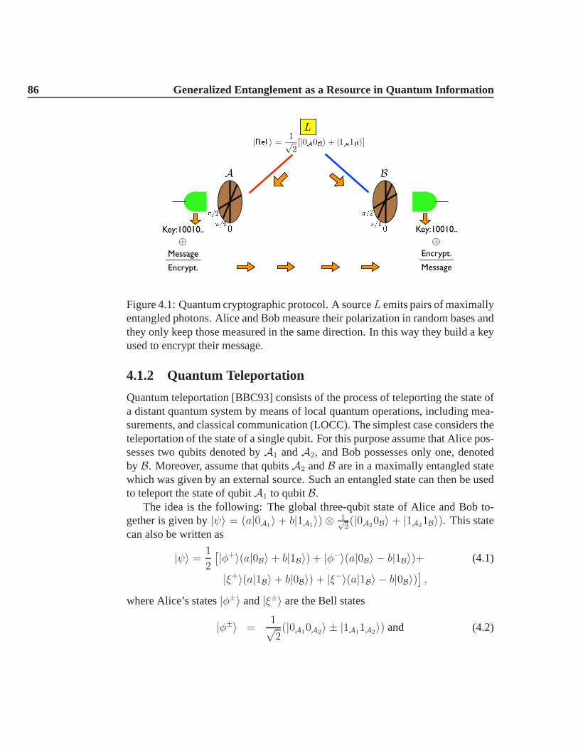
86 Generalized Entanglement as a Resource in Quantum Information
Figure 4.1: Quantum cryptographic protocol. A sourceL emits pairs of maximallyentangled photons. Alice and Bob measure their polarization in random bases andthey only keep those measured in the same direction. In this way they build a keyused to encrypt their message.
4.1.2 Quantum Teleportation
Quantum teleportation [BBC93] consists of the process of teleporting the state ofa distant quantum system by means of local quantum operations, including mea-surements, and classical communication (LOCC). The simplest case considers theteleportation of the state of a single qubit. For this purpose assume that Alice pos-sesses two qubits denoted byA1 andA2, and Bob possesses only one, denotedby B. Moreover, assume that qubitsA2 andB are in a maximally entangled statewhich was given by an external source. Such an entangled state can then be usedto teleport the state of qubitA1 to qubitB.
The idea is the following: The global three-qubit state of Alice and Bob to-gether is given by|ψ〉 = (a|0A1〉 + b|1A1〉) ⊗ 1√
2(|0A20B〉 + |1A21B〉). This state
can also be written as
|ψ〉 = 1
2
[|φ+〉(a|0B〉+ b|1B〉) + |φ−〉(a|0B〉 − b|1B〉)+ (4.1)
|ξ+〉(a|1B〉+ b|0B〉) + |ξ−〉(a|1B〉 − b|0B〉)],
where Alice’s states|φ±〉 and|ξ±〉 are the Bell states
|φ±〉 =1√2(|0A10A2〉 ± |1A11A2〉) and (4.2)
4.2 Quantum Entanglement and Quantum Computation 87
|ξ±〉 =1√2(|0A11A2〉 ± |1A10A2〉),
respectively. Remarkably, in this basis (Eq. 4.2) the stateof Bob’s qubit looks verysimilar to the state to be teleported (i.e., the state ofA1). Then, Alice performs ameasurement in her two qubits projecting them into one of thefour possible Bellstates. (Such a measurement can be done using local operations only but I do notdescribe it here.).
The state obtained by Alice corresponds to one of the four possibilities shownin Eq. 4.2. Alice then contacts Bob and tells him about the result of the measure-ment, after which Bob acts on its qubit to recover the state ofA1. For example, ifAlice projects its two-qubit state into|ξ+〉, then she tells this result (by means of aclassical communication) to Bob. He thereby transforms thestate of his qubit byusing a flip operation transforming
a|1B〉+ b|0B〉 → a|0B〉+ b|1B〉, (4.3)
which is the desired teleported state. Similar operations can be done for any otherstate measured by Alice.
4.2 Quantum Entanglement and Quantum Compu-tation
Perhaps the most important practical case where QE can be used as a resource isin computational tasks. As mentioned before, parallelism is one of the propertiesof the quantum world that needs to be exploited in a quantum computation, andsuch a property is naturally associated to QE. Shor’s factoring algorithm [Sho94]constitutes a nice example where entangled states are used to find the prime fac-tors of a whole number. It has been shown that using a QC, this algorithm canbe efficiently performed; that is, with a number of steps thatscales at most poly-nomially with the integerP to be factorized. However, it is not known how toperform such an algorithm efficiently on a CC: In order to find the factors ofP itis necessary to divide it by all the whole numbers between 1, andP/2, and so on,constituting a time consuming task.
To demonstrate Shor’s algorithm, I present the factorization of the numberP = 15. (Although the solution to this problem is immediately found,P = 15 =3 × 5, this method can be extended to the factorization of larger numbers likeP ′ = 12319, where finding the solution is more complicated:P ′ = 97 × 127.)
88 Generalized Entanglement as a Resource in Quantum Information
As I will show, the problem of finding the factors ofP is equivalent to the order-finding problem. Thus, a random whole numberm between 1 andP − 1 needsto be chosen first. Assume that this number ism = 8. Second, a QA needs tobe performed to find theorder n of m, moduloP . Such order is defined as theleast positive integer such thatmn = 1( modP ), wherea = b( modP ) if a− b isdivisible byP .
Then, the first step of the QA consists of performingr Hadamard gates to theinitial (r+4)-qubit polarized state|01 · · · 0r〉⊗ |0a0b0c0d〉. The numberr of extraqubits has to be big enough to find the ordern with high accuracy [Sho94]. Here,r = 11. The other 4 qubits are necessary to encode information about the factorsof 15 (i.e.,24 = 16 > 15).
After the Hadamard gates have been applied (i.e., the gates that transform|0〉 → |+〉), the evolved state is
|ψ〉 = 1√2r
2r−1∑
j=0
|j〉 ⊗ |0a0b0c0d〉, (4.4)
where|j〉 is the state corresponding to the binary decomposition of the integerjin the logical basis; for example,|j = 3〉 = |01 · · · 1r−10r〉. The next step of thealgorithm is to apply a unitary operation that transforms
|j〉 ⊗ |0a0b0c0d〉 → |j〉 ⊗ |mj( modP )〉. (4.5)
This operation can be efficiently performed using controlled operations on thestate of ther qubits, but I will not explain it here. After this evolution,the evolvedstate is
|ψ〉 =1√2r
2r−1∑
j=0
|j〉 ⊗ |mj( modP )〉 (4.6)
=1√2r
[|0〉 ⊗ |1〉+ |1〉 ⊗ |8〉+ |2〉 ⊗ |4〉+ |3〉 ⊗ |2〉+ · · ·] ,
where again I have chosen the integer representation of the states in the logicalbasis. The state of Eq. 4.6 is a highly entangled state between ther = 11 qubitsand qubitsa, b, c, andd.
By defining the states|µq〉 for qubitsa, b, c, d, as
|µq〉 =1√n
n−1∑
k=0
exp
[−i2πqkn
]|mk( modP )〉, (4.7)

4.2 Quantum Entanglement and Quantum Computation 89
where againn is the not yet known order, Eq. 4.6 can be written as
|ψ〉 = 1√n2r
n−1∑
q=0
2r−1∑
j=0
exp
[i2πqj
n
]|j〉 ⊗ |µq〉. (4.8)
A (inverse) quantum Fourier transform [NC00] performed to the r qubits in theabove state maps it to
1√2r
2r−1∑
j=0
exp
[i2πqj
n
]|j〉 → |K = q/n〉, (4.9)
where the state|K = q/n〉 of ther qubits is a product state which depends on thecoefficientq/n as in the usual Fourier transform. This transformation can alsobe efficiently implemented in a quantum circuit. Therefore,the transformed statereads
|ψ〉 = 1√n
n−1∑
q=0
|K = q/n〉 ⊗ |µq〉. (4.10)
In this way, the register ofr qubits is measured in the logical basis to project thestate|ψ〉 and obtain one possible state|K = q/n〉⊗ |µq〉. After applying the samealgorithm several times and by applying a continued-fractions algorithm, it is pos-sible to obtain the ordern from the statistics of the measured states|K = q/n〉.In this case one would obtainn = 4, such that84 = 4096 = 1( mod15). Sucha solution could be obtained if the result of the measurementin the register ofr qubits gives, for example,|K = q/n〉 = |1536〉 (in the binary representation),where I have used again the integer representation of statesin the logical basis. Ifthis is the case,q/n = 1536
211= 3
4, resulting inn = 4. From this information, one
can obtain that15 = 3× 5 as it is explained in Ref. [Sho94].A factoring QA such as the one presented is more efficient thana classical
one only because entangled states have been created at some step. Otherwise, noadvantages can be gained, in general, from using a deterministic QC. As a simpleexample, suppose (with no loss of generality) that the initial pure state of a registerof N qubits is the usual polarized state|01 · · · 0N〉, and that the QA never doescreate QE. That is, the set of unitary gatesUj applied to the initial state are onlysingle qubit rotations transforming product states into product states. Therefore,
Uj = eiθjσ
α(j)π(j) = cos θ + i sin θσ
α(j)π(j) , (4.11)
90 Generalized Entanglement as a Resource in Quantum Information
whereπ(j) = [1 · · ·N ] denotes the qubit rotated at thejth step, andα(j) =[x, y, z] is the axis of rotation. The evolved state is then
∏
j
Uj |01 · · · 0N〉. (4.12)
After the evolution is performed, certain qubit(s) is(are)measured in, for example,the logical basis. As usual, this is the last step of a deterministic QA (Sec. 2.2). Ifthekth qubit is measured, the result obtained is
〈σkz 〉 = 〈01 · · ·0N |
(∏
j
U †j
)σkz
(∏
j
Uj
)|01 · · · 0N〉. (4.13)
The fact is that such QA can be simulated classically and the expectation valueof Eq. 4.13 can be computed in a CC with the same amount of resources (i.e., sameefficiency). The idea is to only keep track of the informationabout[θj , α(j)] ifπ(j) = k, because the other qubits are not measured. If the QA is performedefficiently, only a polynomially large number of pairs[θj , α(j)] are kept. A clas-sical algorithm to obtain the result of Eq. 4.13 would consist of updating at eachstep the state of thekth qubit only. For example, if at thejth step the state isaj|0k〉 + bj |1k〉 and the gateUj+1 = ei
π4σkx is performed after, the evolved state
becomes
[cos(π/4) + i sin(π/4)σkx](aj|0k〉+ bj |1k〉) = aj+1|0k〉+ bj+1|1k〉, (4.14)
and sinceσkx is the corresponding flip operation,aj+1 =
1√2(aj + ibj) andbj+1 =
1√2(iaj + bj). Updating the values of the complex coefficientsaj andbj can be
easily done with a conventional computer. At the end of the total evolution thestate of thekth qubit isaM |0k〉+ bM |1k〉. Therefore, the result of Eq. 4.13 is
〈σkz 〉 = |aM |2 − |bM |2, (4.15)
which can be efficiently computed with a CC.However, if some of the gatesUj create entanglement, there is no known way,
in general, to classically evaluate Eq. 4.13 efficiently. Naturally, the elementarytwo-qubit gates, like theRzjzk(ω) or the CNOT gate introduced in Sec. 2.1.3,are responsible for creating entanglement. For example, ifthe initial state is theproduct (unentangled) state1√
2|0 + 1〉 ⊗ |0〉, applying the CNOT gate evolves it
into 1√2(|00〉+|11〉), which is known to be one of the Bell states, that is, maximally
entangled. Nonetheless, I will show in the next section thatcreation of QE is not asufficient condition to claim that Eq. 4.13 cannot be obtained efficiently by usinga classical algorithm.

4.3 Efficient Classical Simulations of Quantum Physics 91
4.3 Efficient Classical Simulations of Quantum Physics
The purpose of this section is to generalize the concepts described previously,presenting a wide set of problems which can be solved efficiently with both, aQC or a classical one. To show this, I will exploit the notion of GE, which waspresented in Sec. 3.2. Again, an algorithm is said to be efficient with respect toa certain variableN , whenever the amount of resources required to perform it isbounded by a polynomial inN . Otherwise, the algorithm is said to be inefficient.It is important to remark that here I only make a comparison between efficientand inefficient algorithms, with the previous definition, and do not compare thetotal amount of resources needed. For example, if a QA can be performed inN operations and the corresponding classical one inN2 operations then, despitebeing more convenient to use the former, both are consideredefficient.
In most cases, the type of problems one encounters in quantummechanics arerelated with the evaluation of a certain expectation value or correlation function
〈W 〉 = 〈φ|W |φ〉, (4.16)
whereW is an operator acting on a finite quantum systemS in some state|φ〉 ∈ H.(H is the Hilbert space associated toS.) In Sec. 2.2, I presented some QAs thatallow one to compute Eq. 4.16 in a QC described by the conventional model,whenever the operator algebra associated to the systemS could be mapped ontothe Pauli operators (Sec. 2.3). The main steps of those QAs consist of the prepa-ration of the state|ψ〉 = |+〉a ⊗ |φ〉, from some initial (boot-up) reference statelike |0〉a ⊗ |0 · · ·0〉, then an evolution, and finally the measurement of the ancillaqubita. Similarly, in the rest of this section I assume that the algebra of operatorsused to describe the quantum computational model and/or thealgebra associatedto the systemS are not necessarily described by the conventional model, but aone-to-one efficient mapping between both exists.
Since I am mainly interested in comparing the efficiencies ofobtaining Eq. 4.16using a QC or a classical (conventional) one, the efficiency is defined relative toa certain variableN which here is, in general, the number of quantum mechan-ical elements that compose the systemS. I assume that there exists a QA thatevaluates Eq. 4.16 efficiently, that is, using at most poly(N) resources. These arethe so-calledbounded polynomial quantum algorithms(BPQA). This is usuallyvalid whenever the QC can be efficiently initialized and every step, including thepreparation of|φ〉, can be efficiently performed. These results were previouslydiscussed in Sec. 2.5.

92 Generalized Entanglement as a Resource in Quantum Information
The most common classical algorithm to evaluate Eq. 4.16 consists of writingthe matrix representation ofW , and obtaining the corresponding matrix element.This is usually a hard task because of the dimension of the Hilbert spaceH grow-ing exponentially withN . However, in some cases this complexity can be highlyreduced. The simplest case is when the state|φ〉 of Eq. 4.16 is known to be aneigenstate ofW , so that the corresponding expectation is simply the known eigen-value.
Nonetheless, a more general result can be obtained in a Lie algebraic frame-work. For this purpose, I start by pointing out that, with no loss of generality, thestate|φ〉 ∈ H of Eq. 4.16 can be obtained by transforming any reference state|ref〉 ∈ H; that is
|φ〉 = U |ref〉, (4.17)
whereU † = U−1 (unitary). Moreover, the reference state can be chosen to bethe highest (or lowest) weight state|HW〉 of certain finite semi-simple Lie algebrah = O1, O2, · · · , OM, with Oj = O†
j (Sec. 3.2.2). In this case,h also admitsa Cartan-Weyl decomposition:h = hD, h+, h−, with hD the Cartan subalgebra(CSA) ofh, andh+ andh− the set of raising and lowering operators, respectively(Sec. 3.2.2).
Now suppose that the transformationU of Eq. 4.17 is a group operation in-duced byh; that is
U = exp
[i
M∑
j=1
ζjOj
]. (4.18)
Then|ψ〉 is a GCS and generalized unentangled state (extremal) ofh. Moreover,suppose thatW of Eq. 4.16 can be decomposed as
W =M∑
j=1
κjOj, (4.19)
whereκj ∈ C ∀j, andOj ∈ h. In general,W does not have the form of Eq. 4.19and it belongs to a Lie algebra other thanh. Then,h must be considered as theLie algebra that contains both. (The important case whenW ∈ H ≡ eih, i.e. thegroup induced byh, is discussed in the next section.)
In this way, computing classically Eq. 4.16 is equivalent toevaluating
〈W 〉 =M∑
j=1
κj〈HW|e−i
M∑j=1
ζjOj
Ojei
M∑j=1
ζjOj
|HW〉. (4.20)
4.3 Efficient Classical Simulations of Quantum Physics 93
The operators
O′j = e
−iM∑j=1
ζjOj
Ojei
M∑j=1
ζjOj
=
M∑
j′=1
νjj′Oj′ (4.21)
are also elements inh because they are transformed by a group operation. The co-efficientsνjj′ of Eq. 4.21 can be computed by means of the representation theory.A matrix representationof h is the mappingΦ : h→ C2p such that
Φ(Oj) = Oj, (4.22)
Φ([Oj , Oj′]) =[Φ(Oj),Φ(Oj′)
]=[Oj, Oj′
],
where[A,B] is the commutator and the complex matricesOj arep × p dimen-sional. A representationΦ is said to befaithful when maps linearly independentelements inh to linearly independentp× p matrices. If the Lie algebrah is com-pact, one can always find a faithful representation satisfying the inner product
Tr[OjOj′] = δjj′, (4.23)
with Tr[Q] being the trace ofQ. For example, the well known adjoint represen-tation (Appendix C), which associates anM ×M matrix to every operator inh(M is the dimension ofh), is faithful and satisfies Eq. 4.23. Nevertheless, smallerdimensional faithful representations (p < M) can usually be found. Then, ifΦ isfaithful,
O′j = e
−iM∑j=1
ζjOj
Ojei
M∑j=1
ζjOj
=M∑
j′=1
νjj′Oj′, (4.24)
which is the matrix representation of Eq. 4.21. Since this isa matrix operation,the matricesO′
j of Eq. 4.24 can be classically computed withO(p2) computationaloperations1 (addition and multiplication of complex numbers). Each coefficientνjj′ is then classically obtained by using the inner product equation, that is
νjj′ = Tr[O′jOj′], (4.25)
which also requiresO(p2) computational operations2.1HereO denotes the order of required operations.2To obtainνjj′ at accuracyǫ the order of poly(1/ǫ) operations are needed. Nevertheless, in this
section I consider that the calculation is done at the computational accuracy given by the particulartype of CC used.

94 Generalized Entanglement as a Resource in Quantum Information
Similarly, in the CW basis,
O′j =
r∑
k=1
γjkhk +
l∑
j′=1
ιjj′Eαj′+ ι∗jj′E−αj′
(4.26)
wherehk ∈ hD (CSA),Eαj′∈ h+, andE−αj′
∈ h− (Sec. 3.2.2). The coefficientsγjk andιjj′ of Eq. 4.26 can also be obtained classically withO(p2) computationaloperations by the trace inner product: The operatorshk, Eαj′
, andE−αj′are usu-
ally a simple linear combinations of the operatorsOj.By definition,|HW〉 is an eigenstate of the operators in the CSA, that is
hk|HW〉 = ek|HW〉, (4.27)
where the eigenvaluesek are assumed to be known. Then,
〈HW|Eαj′|HW〉 = 〈HW|E−αj′
|HW〉 = 0 ∀j′. (4.28)
In other words, Eq. 4.20 can be classically computed by only keeping the elementsof O′
j (Eq. 4.21) belonging tohD:
〈HW|O′j|HW〉 =
r∑
k=1
γjk〈HW|hk|HW〉 =r∑
k=1
γjkek, (4.29)
and
〈W 〉 =M∑
j=1
r∑
k=1
κjγjkek. (4.30)
Since the coefficientsek are assumed to be known, and the coefficientsκj andγjkcan be classically obtained withO(p2), Eq. 4.30 can be computed withO(Mrp2)computational operations. IfM ≤ poly(N), thenr ≤ poly(N). Also, the exis-tence of the adjoint representation (Appendix C) guarantees that one can alwaysfind p such thatp ≤ M ≤ poly(N). Therefore, Eq. 4.30 can be efficiently com-puted with a conventional computer. A more detailed proof about the numberof operations required, including the approximation of theexponential matrix, isgiven in the Appendix E.
In brief, when the state|φ〉 of Eq. 4.16 is a GCS of a polynomially largedimensional Lie algebrah, and the operatorW is an element ofh, Eq. 4.16 can beefficiently computed with both, a classical and a quantum device.

4.3 Efficient Classical Simulations of Quantum Physics 95
However, in some casesW or U (Eq. 4.17) are associated with an exponen-tially large dimensional Lie algebra and the correspondingclassical simulation isinefficient. Nevertheless, it is important to remark that for mixed states of the form
ρ =L∑
s=1
psρs, (4.31)
whereρs = |φs〉〈φs|, and|φs〉 being GCSs and generalized unentangled states ofa polynomially large dimensional Lie algebra, the computation of
〈W 〉 = Tr(ρW ), (4.32)
can also be efficiently performed with a CC ifL ≤ poly(N).
4.3.1 Higher Order Correlations
The previous results can be extended to the computation of higher order correla-tions. For simplicity, I start by studying the case of two-body correlations of theform
〈W 〉 = 〈φ|W1W2|φ〉, (4.33)
whereW is the product of the observablesW1 = W †1 andW2 = W †
2 . Again,W1
andW2 are considered to be elements of a Lie algebrah = O1, · · · , OM, and|φ〉 is assumed to be a GCS ofh; that is
|φ〉 = U |HW〉, (4.34)
with U = exp[i∑
j ζjOj
], and|HW〉 the highest weight state ofh. In this way,
Eq. 4.33 reads〈φ|W1W2|φ〉 = 〈HW|U †W1W2U |HW〉. (4.35)
SinceUU † = 1l,〈φ|W1W2|φ〉 = 〈HW|W ′
1W′2|HW〉, (4.36)
whereW ′i = U †WiU .
Equation 4.33 can be efficiently computed with a classical computer if thedimensionM of h scales at most polynomially with the variableN ; i.e. M ≤poly(N). To show this, I first decompose the corresponding operatorsas
W1 =
M∑
j=1
κ1j Oj, (4.37)

96 Generalized Entanglement as a Resource in Quantum Information
W2 =M∑
j=1
κ2jOj, (4.38)
which transform under the action ofU as
W ′i = U †WiU =
M∑
j=1
κijO′j ; i = 1, 2. (4.39)
In a CW basis ofh, the transformed observablesO′j = U †OjU can be decom-
posed as in Eq. 4.26. Such decomposition can be done efficiently with a CC (i.e.,computing the coefficientsγjk and ιjj′) by working in low-dimensional faithfulrepresentation ofh (Appendix C). Then,
〈W1W2〉 =M∑
i,j=1
κ1iκ2j〈HW|O′
iO′j|HW〉, (4.40)
with
〈HW|O′iO
′j| HW〉 =
r∑k,k′=1
γikγjk′〈hkhk′〉+l∑
i′,j′=1
[ιii′ιjj′〈Eαi′
Eαj′〉
+ C.C.+ ιii′ι∗jj′〈Eαi′
E−αj′〉+ ι∗ii′ιjj′〈E−αi′
Eαj′〉]
+r∑
k=1
l∑j′=1
[γikιjj′〈hkEαj′
〉+ γikι∗jj′〈hkE−αj′
〉+ C.C.], (4.41)
where C.C. denotes the complex conjugate, and the expectation values are nowtaken over the highest weight state, i.e.〈A〉 = 〈HW|A|HW〉. Since raising oper-ators annihilate|HW〉 only a few expectations do not vanish in Eq. 4.41. Theseare
〈hkhk′〉 = ekek′ , (4.42)
〈Eαj′E−αj′
〉 = 〈E−αj′Eαj′
+
r∑
k=1
αkj′hk〉 =
r∑
k=1
αkj′ek, (4.43)
where the coefficientsαkj are the components of the root vectorαj (Sec. 3.2.2)
andek are the known weights of|HW〉.In brief, Eq. 4.33 takes the form
〈φ|W1W2|φ〉 =M∑
i,j=1
κ1iκ2j
[r∑
k,k′=1
γikγjk′ekek′ +
l∑
j′=1
r∑
k=1
ιij′ι∗jj′α
kj′ek
], (4.44)
4.4 Generalized Entanglement and Quantum Computation 97
which can be efficiently computed with a CC ifM ≤ poly(N).Higher order correlation functions of the form
〈W 〉 = 〈φ|W p · · · W 1|φ〉 (4.45)
can also be computed efficiently for a fixed integerR, whenever there is a polyno-mially large dimensional Lie algebrah associated to the problem. Obviously, thecomplexity of this problem increases asp does. Again, the idea is to keep onlythe nonzero expectations of the transformed operatorW ′ = U †W p · · · W 1U =W ′p · · · W ′1, where|φ〉 = U |HW〉. For this purpose, all the raising operatorsEαj
appearing inW ′ must be taken to the right side, by using the commutationrelations of the algebra, so that they destroy the state|HW〉. This problem isanalogous to the one given by Wick’s theorem [Wic50] for fermionic operators.In Appendix F, I describe an efficient method for the classical computation ofEq. 4.45.
4.4 Generalized Entanglement and Quantum Com-putation
In Sec. 4.3 I presented a class of classical algorithms that allows one to efficientlyobtain certain correlation functions of quantum systems ina conventional com-puter. Here, I analyze some advantages of having a QC. For example, assumethen that one is interested in the evaluation of the correlation function of Eq. 4.16,when there is no polynomially large dimensional Lie algebrah associated withthe problem. That is, either|φ〉 is not a GCS ofh or W is not an element orgroup element induced byh. Then, if abounded polynomial quantum algorithm(BPQA) like the ones introduced in Sec. 2.2 exists in this case, Eq. 4.16 can beefficiently computed using a QC. Usually, no known classicalalgorithm can beused to compute such a correlation efficiently and this represents, in some cases,an exponential speed-up of the quantum simulation with respect to the classicalone.
In Sec. 2.5, I discussed the complexity of simulating physical systems us-ing QCs. Although certain QSs have been shown to be efficient,others, like theobtention of the ground state properties in the two-dimensional Hubbard model,remained inefficient. The problem relied in the complexity of preparing the de-sired initial state|φ〉. When simulating quantum systems, this state is usuallynot completely known (e.g., it is the ground state of some non-solvable Hamilto-nian) and an approximated state, having a non-zero overlap with |φ〉, needs to be
98 Generalized Entanglement as a Resource in Quantum Information
prepared. The purpose of the following section is then to show a wide class ofquantum states that can be prepared efficiently by quantum networks. Again, theresults obtained are independent of the physical representation of the QC when-ever an efficient mapping between the operators used to describe the system to besimulated and the operators describing the computational model, exists.
4.4.1 Efficient Initial State Preparation
I start by describing the simple case when the initial state to be prepared is givenby
|φ〉 = U |HW〉, (4.46)
where|HW〉 is the highest weight of some Lie algebrah, and is considered tobe the boot-up state of the computer, which can be efficientlyinitialized. If theoperatorU of Eq. 4.46 is a group operation induced byh, that is,U = eiA andA ∈ h = O1, · · · , OM, andM ≤ poly(N), then|φ〉 can be prepared efficientlywith arbitrary accuracy by using, for example, a first order Trotter decomposi-tion [Suz93]. In this case, the state|φ〉 is generalized unentangled and GCS ofh.Then,A =
∑Mj=1 ζjOj and
eiA =∏
eiA∆t, (4.47)
eiA∆t ≈M∏
j=1
eiζjOj∆t. (4.48)
Assuming that every operationeiζjOj∆t is either an elementary gate or can beperformed by applying a small number of them, the evolutioneiA can be thenapproximated by applying a polynomially large number of these gates. Particularexamples were discussed in Sec. 2.3.
Another interesting case is when the state|φ〉 is not given in the form ofEq. 4.46 but some information, like the expectation values of a set of observ-ables (i.e., its reduced state),〈Oj〉, is known or can be easily obtained. Ifh =
O1, · · · , OM is a semi-simple Lie algebra, withM ≤ poly(N), and|φ〉 is shownto be a GCS ofh by calculating, for example, theh-purity (Sec. 3.2.2), then it canbe prepared efficiently with a QC. To show this, one needs to obtain first the op-eratorA =
∑Mj=1 ζjOj such thatU = eiA is the transformation of Eq. 4.46.

4.4 Generalized Entanglement and Quantum Computation 99
For this purpose, I define the fictitious Hamiltonian
HF = −M∑
j=1
〈Oj〉Oj, (4.49)
whose expectation value over the state|ψ〉 is
〈ψ|HF |ψ〉 = −M∑
j=1
〈Oj〉2. (4.50)
If |ψ〉 = V |ψ〉 is another GCS ofh, with V a unitary group operation that trans-forms as
V †OjV =M∑
j′=1
νjj′Oj′, (4.51)
then
〈ψ|HF |ψ〉 = −M∑
j,j′=1
〈Oj〉νjj′〈Oj′〉. (4.52)
Since theM ×M matrix defined by the real coefficientsνjj′ is orthogonal, oneobtains (Schur’s inequality)
〈ψ|HF |ψ〉 ≥ 〈ψ|HF |ψ〉. (4.53)
Therefore,|ψ〉 is the unique GCS and ground state that minimizes such expecta-tion value.
Assume now thatHF can be efficiently diagonalized with a conventional com-puter, obtaining
HF = UH0U†, (4.54)
whereU is a unitary group operation and
H0 =
r∑
k=1
γkhk , (4.55)
is an unperturbed Hamiltonian (i.e.,hk are elements in the CSA ofh). Such adiagonalization algorithm is described in Sec. 5.2.1. Defining |ψ〉 = U †|ψ〉, oneobtains
〈ψ|HF |ψ〉 = 〈ψ|H0|ψ〉, (4.56)

100 Generalized Entanglement as a Resource in Quantum Information
which takes its minimum value, by definition, for a certain weight state|φ〉. Inparticular, the coefficientsγk of Eq. 4.55 can be chosen such that|ψ〉 = |HW〉 (seeChap. 5). Therefore,|ψ〉 = U |HW〉, andU is the desired group operation. Again,U can be approximated by applying a polynomially large numberof elementarygates so|ψ〉 can be prepared efficiently with a QC.
4.5 Summary
In this chapter I have addressed several issues relating theconcept of GE withquantum and classical complexity. I have shown that the creation of GE relativeto every polynomially large dimensional Lie algebra is a necessary requirement togain efficiency over the known classical algorithms. Otherwise, efficient classicalsimulations exist, which realize the computation by working in low-dimensionalrepresentations of the algebra. This result goes beyond therequirement of creatingentangled states in the usual sense. For example, a quantum algorithm involvinggates induced by the Lie algebrah = so(2N), which is presented in detail in thenext chapter, creates entangled states in the standard sense (i.e., non-separable).However, since the dimension ofh is polynomially large, such quantum computa-tion can be efficiently simulated with a CC.
The efficient preparation of a wide class of states by quantumnetworks hasalso been studied. Again, any GCS or generalized unentangled state of a polyno-mially large dimensional Lie algebra can be efficiently prepared on a QC.
Chapter 5
Generalized Entanglement andMany-Body Physics
Information is inevitably physical.
Rolf Landauer
Every QC has associated certain physical representation (e.g., spin-1/2 system,etc.). The fact that information is not just an abstract entity and is always linkedto a physical system, implies that it must be governed by the laws of physics.In Quantum Information Theory, for example, the manipulation and control ofinformation is based on the foundations and laws of the quantum mechanics. Onthe other hand, many concepts, such as QE, have been developed only from aninformation-theory point of view. It is expected then that these concepts are alsouseful for the analysis of physical phenomena. In this chapter, I apply the notionof GE (Chap. 3) to the study of different problems in many-body physics.
First, I will focus on the characterization of quantum phasetransitions (QPTs)in matter. QPTs are qualitative changes occurring in the properties of the groundstate of a many-body system due to modifications either in theinteractions amongits constituents or in their interactions with an external probe [Sac99], while thesystem remains at zero temperature. Typically, such changes are induced as a pa-rameterg in the system HamiltonianH(g) is varied across a point at which thetransition is made from one quantum phase to a different one.Often some cor-relation length diverges at this point, in which case the latter is called aquantumcritical point. Because thermal fluctuations are inhibited, QPTs are purely drivenby quantum fluctuations. Thus, these are purely quantum phenomena: A classicalsystem in a pure state cannot exhibit quantum correlations.Prominent examples
102 Generalized Entanglement and Many-Body Physics
of QPTs are the quantum paramagnet to ferromagnet transition occurring in Isingspin systems under an external transverse magnetic field [LSM61, Pfe70, BM71],the superconductor to insulator transition in high-Tc superconducting systems, andthe superfluid to Mott insulator transition originally predicted for liquid heliumand recently observed in ultracold atomic gases [GME02].
Since entanglement is a property inherent to quantum statesand intimatelyrelated to quantum correlations (Chap. 3), one would expectthat, in some appro-priately defined sense, the entanglement present in the ground state undergoes asubstantial change across a point where a QPT occurs. Thus, the concept of GEbecomes specially well suited for this study because it is directly applicable to anyalgebraic language associated to the system under study.
Another important problem in quantum mechanics is to exactly diagonalizeand obtain the spectrum of a Hamiltonian of a many-body system. In this case, noapproximate methods (e.g., mean field theory) are needed andone has completeknowledge of the physical properties of the system through algebraic methods.By using information-theory concepts such as the ones described for the efficientsimulation of physical systems (Sec. 4.3), I will show that whenever there is a Liealgebraic structure behind a problem in quantum physics, and the dimension ofthe associated Lie algebra is small enough, such problems can be solved easilyby using a CC. This constitutes the final part of my thesis after which come theconclusions (Chap. 6).
5.1 Entanglement and Quantum Phase Transitions
In this section, I characterize the QPTs present in the Lipkin-Meshkov-Glick(LMG) model and in the anisotropic XY model in an external magnetic fieldthrough the GE notion, relative to a particular subset of observables which willbe appropriately chosen in each case. Interestingly, for both of these models theground states can be computed exactly by mapping the set of observable opera-tors involved in the system Hamiltonian to a new set of operators which satisfy thesame commutation relations; thus, preserving the underlying algebraic structure.In the new operator language, the models are seen to contain some symmetriesthat make them exactly solvable, allowing one to obtain the ground state proper-ties in a number of operations that scales polynomially withthe system size. It ispossible then to understand which quantum correlations give rise to the QPTs inthese cases.
Several issues should be considered when looking for an algebrah of observ-
5.1 Entanglement and Quantum Phase Transitions 103
ables that may make the corresponding relative purity a goodindicator of a QPT.First, one observes that in each of these cases a preferred Lie algebra exists, wherethe respective ground state would have maximumh-purity independently of theinteraction strengths in the Hamiltonian. The purity relative to such an algebra re-mains constant, therefore it does not identify the QPT. (In these cases, this algebrais in fact the Lie algebra generated by the parametrized family of model Hamil-tonians, as the parameters are varied.) Thus, one needs to extract a subalgebrarelative to which the ground state may be generalized entangled, depending onthe parameters in the Hamiltonian. A second, closely related observation is thatthe purity must contain information about quantum correlations which undergo aqualitative change as the transition point is crossed: thus, the corresponding de-gree of entanglement, as measured by the purity, must dependon the interactionstrengths governing the phase transition. Finally, whenever a degeneracy of theground state exists or emerges in the thermodynamic limit, aphysical requirementis that the purity be the same for all ground states.
Although these restrictions together turn out to be sufficient for choosing therelevant algebra of observables in the following two models, they do not pro-vide an unambiguous answer when solving a non-integrable model whose exactground state solution cannot be computed efficiently. Typically, in the latter casesthe ground states are GCSs of Lie algebras for each of which the dimension in-creases exponentially with the system size. Choosing the observable subalgebrathat contains the proper information on the QPTs (such as information on criticalexponents) then becomes, in general, a difficult task.
A concept ofgeneral mean-field Hamiltonians(GMFH) emerges from theseconsiderations. Given a Hilbert spaceH of dimensionpN (with p an integer> 1),I define a GMFH as the Hermitian operator
HMF =∑
α
κjOj , κj ∈ R , (5.1)
which is an element of an irreducibly represented Lie algebra of Hermitian opera-torsh = O1, · · · , OM, whose dimension scales at most polynomially inN thatis,M ≤ poly(N). When the ground state ofHMF is non-degenerate, it turns out tobe a GCS ofh [BKO03], while the remaining eigenstates (some of which mayalsobe GCSs) and energies can be efficiently computed. The connection between Lie-algebraic mean-field Hamiltonians and their efficient solvability deserves carefulanalysis in its own right, and will be presented in the following section.
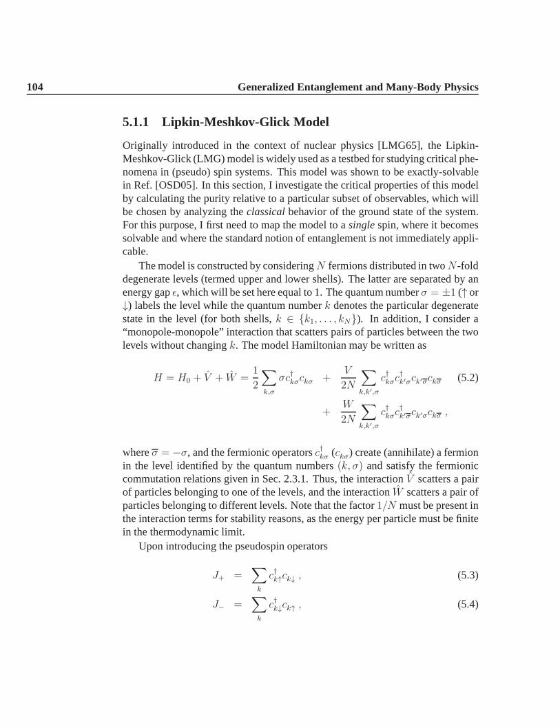
104 Generalized Entanglement and Many-Body Physics
5.1.1 Lipkin-Meshkov-Glick Model
Originally introduced in the context of nuclear physics [LMG65], the Lipkin-Meshkov-Glick (LMG) model is widely used as a testbed for studying critical phe-nomena in (pseudo) spin systems. This model was shown to be exactly-solvablein Ref. [OSD05]. In this section, I investigate the criticalproperties of this modelby calculating the purity relative to a particular subset ofobservables, which willbe chosen by analyzing theclassicalbehavior of the ground state of the system.For this purpose, I first need to map the model to asinglespin, where it becomessolvable and where the standard notion of entanglement is not immediately appli-cable.
The model is constructed by consideringN fermions distributed in twoN-folddegenerate levels (termed upper and lower shells). The latter are separated by anenergy gapǫ, which will be set here equal to 1. The quantum numberσ = ±1 (↑ or↓) labels the level while the quantum numberk denotes the particular degeneratestate in the level (for both shells,k ∈ k1, . . . , kN). In addition, I consider a“monopole-monopole” interaction that scatters pairs of particles between the twolevels without changingk. The model Hamiltonian may be written as
H = H0 + V + W =1
2
∑
k,σ
σc†kσckσ +V
2N
∑
k,k′,σ
c†kσc†k′σck′σckσ (5.2)
+W
2N
∑
k,k′,σ
c†kσc†k′σck′σckσ ,
whereσ = −σ, and the fermionic operatorsc†kσ (ckσ) create (annihilate) a fermionin the level identified by the quantum numbers(k, σ) and satisfy the fermioniccommutation relations given in Sec. 2.3.1. Thus, the interaction V scatters a pairof particles belonging to one of the levels, and the interaction W scatters a pair ofparticles belonging to different levels. Note that the factor 1/N must be present inthe interaction terms for stability reasons, as the energy per particle must be finitein the thermodynamic limit.
Upon introducing the pseudospin operators
J+ =∑
k
c†k↑ck↓ , (5.3)
J− =∑
k
c†k↓ck↑ , (5.4)

5.1 Entanglement and Quantum Phase Transitions 105
Jz =1
2
∑
k,σ
σc†kσckσ =1
2
(n↑ − n↓
), (5.5)
which satisfy thesu(2) commutation relations of the angular momentum algebra,
[Jz, J±] = ±J± , (5.6)
[J+, J−] = Jz , (5.7)
the Hamiltonian of Eq. 5.2 may be rewritten as
H = Jz +V
2N(J2
+ + J2−) +
W
2N(J+J− + J−J+) . (5.8)
As defined by Eq. 5.8,H is invariant under theZ2 inversion symmetry operationK that transforms(Jx, Jy, Jz) 7→ (−Jx,−Jy, Jz), and it also commutes with the(Casimir) total angular momentum operatorJ
2 = J2x + J2
y + J2z . Therefore, the
non-degenerate eigenstates ofH are simultaneous eigenstates of bothK andJ2,and they may be obtained by diagonalizing matrices of dimension2J+1 (wherebythe solubility of the model). Notice that, by definition ofJz as in Eq. 5.5, themaximum eigenvalue ofJz andJ = |J| isN/2. In particular, for a system withNfermions as assumed, both the ground state|g〉 and the first excited state|e〉 belongto the largest possible angular momentum eigenvalueJ = N/2 [LMG65] (so-called half-filling configurations); thus, they can be computed by diagonalizing amatrix of dimensionN + 1.
The Hamiltonian of Eq. 5.8 does not exhibit a QPT for finiteN . It is importantto remark that some critical properties of the LMG model in the thermodynamiclimit N → ∞ can be understood by using a semiclassical approach (note thatthe critical behavior is essentially mean-field): first, I replace the angular momen-tum operators inH/N (with H given in Eq. 5.8) by their classical components(Fig. 5.1); that is
J = (Jx, Jy, Jz) → (J sin θ cosφ, J sin θ sin φ, J cos θ) , (5.9)
H/N → hc(j, θ, φ) , (5.10)
wherehc is the resulting classical Hamiltonian andj = J/N , j = 0, . . . , 1/2. Inthis way, one can show that in the thermodynamic limit (Appendix G)
limN→∞
〈g|H|g〉N
= limN→∞
Eg
N= min
j,θ,φhc(j, θ, φ) , (5.11)
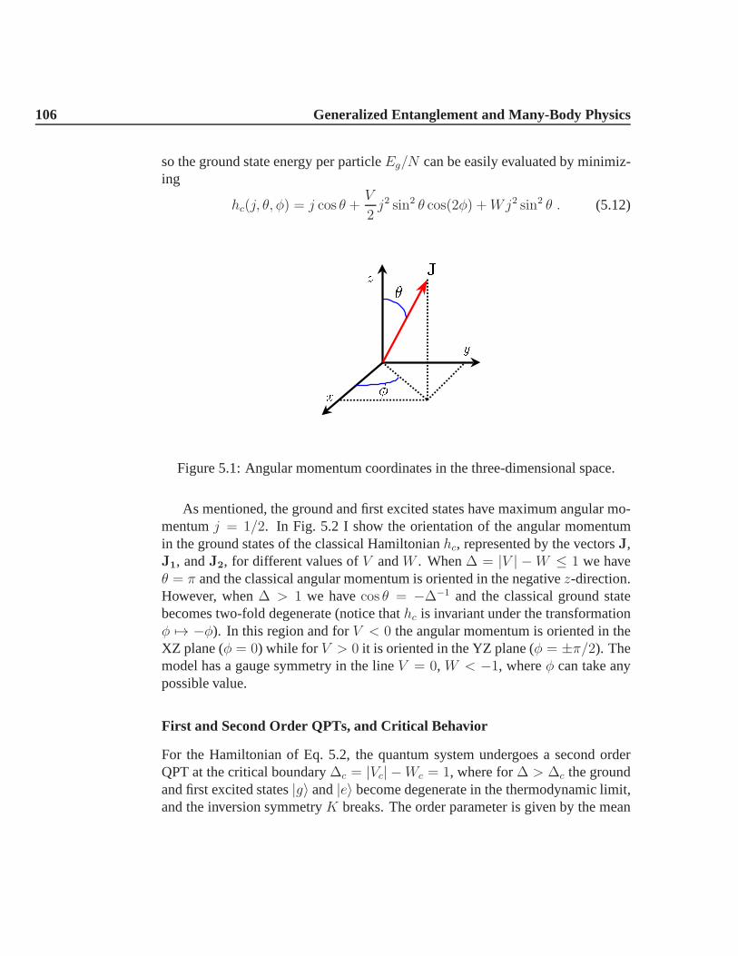
106 Generalized Entanglement and Many-Body Physics
so the ground state energy per particleEg/N can be easily evaluated by minimiz-ing
hc(j, θ, φ) = j cos θ +V
2j2 sin2 θ cos(2φ) +Wj2 sin2 θ . (5.12)
y
x
z
J
Figure 5.1: Angular momentum coordinates in the three-dimensional space.
As mentioned, the ground and first excited states have maximum angular mo-mentumj = 1/2. In Fig. 5.2 I show the orientation of the angular momentumin the ground states of the classical Hamiltonianhc, represented by the vectorsJ,J1, andJ2, for different values ofV andW . When∆ = |V | −W ≤ 1 we haveθ = π and the classical angular momentum is oriented in the negativez-direction.However, when∆ > 1 we havecos θ = −∆−1 and the classical ground statebecomes two-fold degenerate (notice thathc is invariant under the transformationφ 7→ −φ). In this region and forV < 0 the angular momentum is oriented in theXZ plane (φ = 0) while for V > 0 it is oriented in the YZ plane (φ = ±π/2). Themodel has a gauge symmetry in the lineV = 0, W < −1, whereφ can take anypossible value.
First and Second Order QPTs, and Critical Behavior
For the Hamiltonian of Eq. 5.2, the quantum system undergoesa second orderQPT at the critical boundary∆c = |Vc| −Wc = 1, where for∆ > ∆c the groundand first excited states|g〉 and|e〉 become degenerate in the thermodynamic limit,and the inversion symmetryK breaks. The order parameter is given by the mean

5.1 Entanglement and Quantum Phase Transitions 107
z
y
x
J
=
z
y
x
J
2
J
1
<
= 0
z
y
x
J
1
J
2
<
= =2
1
1
1
V > 0
W > 0
( > 1) ( < 1)
(
= 1)
= jV j W
2
nd
order
2
nd
order
1
st
order
`ORDER'
`ORDER'
`DISORDER'
Figure 5.2: Representation of the classical ground state ofthe LMG model.
number of fermions in the upper shell〈n↑〉 = 1/2 + 〈Jz〉/N , which in the ther-modynamic limit converges to its classical value,
limN→∞
〈n↑〉 =1 + cos θ
2. (5.13)
Obviously, for∆ ≤ ∆c one has〈n↑〉 = 0, and〈n↑〉 > 0, otherwise (Fig. 5.2). Thecritical exponents of the order parameter are easily computed by making a Taylorexpansion near the critical points (∆→ 1+). Defining the quantitiesx = Vc − Vandy =Wc −W , one obtains
lim∆→1+
〈n↑〉 =
(yα − xβ)/2 for V > 0(yα + xβ)/2 for V < 0
,
where the critical exponents areα = 1 andβ = 1.In Fig. 5.3 I show the exact ground state energy per particleEg/N (with Eg =
〈g|H|g〉) as a function ofV andW in the thermodynamic limit (Eqs. 5.11). Onecan see that also in the broken symmetry region (∆ > 1) the system undergoes

108 Generalized Entanglement and Many-Body Physics
a first order QPT atV = 0; that is, the first derivative of the ground state energywith respect toV is not continuous in this line.
Figure 5.3: Ground state energy per particle in the LMG model.
Purity as an Indicator of the QPTs in the LMG Model
The standard notion of entanglement is not directly applicable to the LMG modelas described by Eq. 5.8, as this is a single spin system and no physically naturalpartition into subsystems is possible. Therefore, using the h-purity as a measure

5.1 Entanglement and Quantum Phase Transitions 109
of entanglement becomes an advantage from this point of view, since the latteronly depends on a particular subset of observables and no partition of the systemis necessary. The first required step is the identification ofa relevant Lie algebraof observables relative to which the purity has to be calculated.
Since both the ground and first excited states of the quantum LMG model maybe understood as states of a system carrying total angular momentumJ = N/2, afirst possible algebra to consider is thesu(N + 1) algebra acting on the relevant(N + 1)-dimensional eigenspace. Relative to this algebra,|g〉 is generalized un-entangled for arbitrary values ofV andW , thus the corresponding purity remainsconstant and does not signal the QPTs. However, the family ofHamiltonians ofEq. 5.8 do not generate this Lie algebra, but rather ansu(2) algebra.
Thus a natural choice, suggested by the commutation relationships of Eqs. 5.6and 5.7, is to study the purity relative to the spin-N/2 representation of the angularmomentum Lie algebrah = su(2) = Jx, Jy, Jz:
Ph(|ψ〉) =4
N2
[〈Jx〉2 + 〈Jy〉2 + 〈Jz〉2
], (5.14)
where the normalization factorK = N2/4 is chosen to ensure that the maximumof Ph is equal to 1 (Eq. 3.32). With this normalization factor,Ph can be calculatedexactly in the thermodynamic limit by relying on the semi-classical approach de-scribed earlier (Appendix G and Eq. 5.9). ForV = 0 and arbitraryW > 0,|g〉 = |Jz = −N/2〉 which is a GCS ofsu(2) and hasPh = 1. For generic interac-tion values such that∆ ≤ 1, the classical angular momentum depicted in Fig. 5.2is oriented along thez direction and is not degenerate: Because〈Jx〉 = 〈Jy〉 = 0,only 〈Jz〉 contributes toPh. By recalling thatlimN→∞〈Jz/N〉 = −1/2, this givesPh = 1, so thatas far as relative purity is concerned the ground state behavesasymptotically like a coherent state in the thermodynamic limit. Physically, thismeans that with respect to the relevant fluctuations, GCSs ofsu(2) are a goodapproximation of the quantum ground state for large particle numbers, as is wellestablished for this model [GF78]. However, in the region∆ > 1 the ground state(both classical and quantum) is two-fold degenerate in theN →∞ limit, and thevalue ofPh depends in general on the particular linear combination of degeneratestates. This can be understood from Fig. 5.2, where different linear combinationsof the two degenerate vectorsJ1 andJ2 imply different values of〈Jx〉 for V < 0and different values of〈Jy〉 for V > 0, while 〈Jz〉 remains constant. With thesefeatures, the purity relative to thesu(2) algebra will not be a good indicator of theQPT.
An alternative option is then to look at a subalgebra ofsu(2). In particular, if

110 Generalized Entanglement and Many-Body Physics
I only consider the purity relative to the single observableh = so(2) = Jz (i.e.,a particular CSA ofsu(2)), and retain the same normalization as above, then
Ph(|ψ〉) =4
N2〈Jz〉2 . (5.15)
This new purity will be a good indicator of the QPT, sincePh = 1 only for∆ ≤ 1in the thermodynamic limit, and in additionPh does not depend on the particularlinear combination of the two-fold degenerate states in theregion∆ > 1, wherePh < 1. Obviously, in this casePh is straightforwardly related to the order param-eter (Eq. 5.13); the critical exponents ofPh − 1 are indeed the same (α = 1 andβ = 1).
In the region∆ < 1 wherePh = 1, the quantum ground state of the LMGmodel (Eq. 5.8) does not have a well definedz-component of angular momentumexcept atV = 0 ([H, Jz] 6= 0 if V 6= 0), thus in general it does not lie on acoherent orbit of this algebra for finiteN . However, as discussed above, it behavesasymptotically (in the infiniteN limit) as a GCS (in the sense thatPh→ 1).
In Fig. 5.4 I show the behavior ofPh as a function of the parametersV andW . The purity relative toJz is then a good indicator not only of the second orderQPT but also of the first order QPT (the lineV = 0,W < −1).
5.1.2 Anisotropic XY Model in a Transverse Magnetic Field
In this section, I exploit the purity relative to theu(N) algebra (introduced inSec. 3.3.3) as a measure of GE which is able to identify the paramagnetic-to-ferromagnetic QPT in the anisotropic one-dimensional spin-1/2 XY model in atransverse magnetic field and classify its universality properties.
The model Hamiltonian for a chain ofN sites is given by (Fig. 5.5)
H = −gN∑
i=1
[(1 + γ)σi
xσi+1x + (1− γ)σi
yσi+1y
]+
N∑
i=1
σiz , (5.16)
where the operatorsσiα (α = x, y, z) are the Pauli spin-1/2 operators on sitei
(Sec. 2.1),g is the parameter one may tune to drive the QPT, and0 < γ ≤ 1 is theamount of anisotropy in the XY plane. In particular, forγ = 1, Eq. 5.16 reducesto the Ising model in a transverse magnetic field [Pfe70], while for γ → 0 themodel becomes isotropic. Periodic boundary conditions areconsidered here, thatis σi+N
α = σiα, for all i andα.

5.1 Entanglement and Quantum Phase Transitions 111
Figure 5.4: Purity relative to the observableJz in the ground state of the LMGmodel.
Wheng ≫ 1 andγ = 1 the model is Ising-like. In this limit, the spin-spininteractions are the dominant contribution to the Hamiltonian (Eq. 5.16), and theground state becomes degenerate in the thermodynamic limit, exhibiting ferro-magnetic long-range order correlations in thex direction:M2
x = limN→∞〈σ1xσ
N/2x 〉 >
0, whereMx is the magnetization in thex direction. In the opposite limit whereg → 0, the external magnetic field becomes important, the spins tend to alignin the z direction, and the magnetization in thex direction vanishes:M2
x =
limN→∞〈σ1xσ
N/2x 〉 = 0. Thus, in the thermodynamic limit the model is subject
to a paramagnetic-to-ferromagnetic second order QPT at a critical point gc that
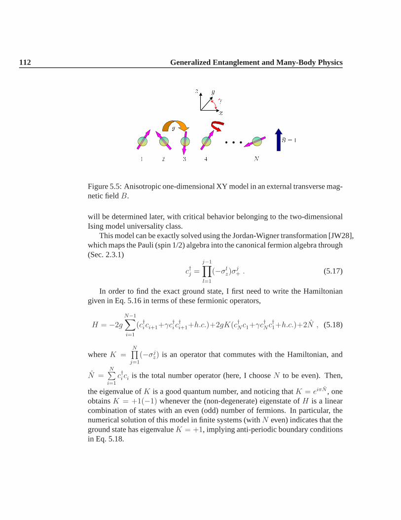
112 Generalized Entanglement and Many-Body Physics
1 2 3 4 N
g
B = 1
x
y
z
Figure 5.5: Anisotropic one-dimensional XY model in an external transverse mag-netic fieldB.
will be determined later, with critical behavior belongingto the two-dimensionalIsing model universality class.
This model can be exactly solved using the Jordan-Wigner transformation [JW28],which maps the Pauli (spin 1/2) algebra into the canonical fermion algebra through(Sec. 2.3.1)
c†j =j−1∏
l=1
(−σlz)σ
j+ . (5.17)
In order to find the exact ground state, I first need to write theHamiltoniangiven in Eq. 5.16 in terms of these fermionic operators,
H = −2gN−1∑
i=1
(c†ici+1+γc†ic
†i+1+h.c.)+2gK(c†Nc1+γc
†Nc
†1+h.c.)+2N , (5.18)
whereK =N∏j=1
(−σjz) is an operator that commutes with the Hamiltonian, and
N =N∑i=1
c†ici is the total number operator (here, I chooseN to be even). Then,
the eigenvalue ofK is a good quantum number, and noticing thatK = eiπN , oneobtainsK = +1(−1) whenever the (non-degenerate) eigenstate ofH is a linearcombination of states with an even (odd) number of fermions.In particular, thenumerical solution of this model in finite systems (withN even) indicates that theground state has eigenvalueK = +1, implying anti-periodic boundary conditionsin Eq. 5.18.

5.1 Entanglement and Quantum Phase Transitions 113
The second step is to rewrite the Hamiltonian in terms of the fermionic opera-tors c†k (ck), defined by the Fourier transform of the operatorsc†j (cj):
c†k =1√N
N∑
j=1
e−ikjc†j , (5.19)
where the setV of possiblek is determined by the anti-periodic boundary con-ditions in the fermionic operators:V = V+ + V− = [± π
N,±3π
N, · · · ,± (N−1)π
N].
Therefore,
H +N = −2∑
kǫV
(−1 + 2g cos k)c†kck + igγ sin k(c†−kc†k + c−kck) . (5.20)
The third and final step is to diagonalize the Hamiltonian of Eq. 5.20 using theBogolubov canonical transformation [BR86]
γk = ukck − ivkc†−k
γ†−k = ukc†−k − ivkck
,
where the real coefficientsuk andvk satisfy the relations
uk = u−k, vk = −v−k , and u2k + v2k = 1 , (5.21)
with
uk = cos(φk
2
), vk = sin
(φk
2
), (5.22)
andφk given by
tan(φk) =2gγ sin k
−1 + 2g cos k. (5.23)
In this way, the quasiparticle creation and annihilation operatorsγ†k andγk,also satisfy the canonical fermionic anti-commutation relations of Eq. 2.34, andthe Hamiltonian may be finally rewritten as
H =∑
kǫV
ξk(γ†kγk − 1/2) , (5.24)
whereξk = 2√(−1 + 2g cos k)2 + 4g2γ2 sin2 k is the quasiparticle energy. Since
in generalξk > 0, the ground state is the quantum state with no quasiparticles(BCS state [Tak99]), such thatγk|BCS〉 = 0. Thus, one finds
|BCS〉 =∏
kǫV+
(uk + ivkc†kc
†−k)|vac〉 , (5.25)

114 Generalized Entanglement and Many-Body Physics
where|vac〉 is the state with no fermions (ck|vac〉 = 0).Excited states with an even number of fermions (K = +1) can be obtained
applying pairs of quasiparticle creation operatorsγ†k to the|BCS〉 state. However,one should be more rigorous when obtaining excited states with an odd number ofparticles, sinceK = −1 implies periodic boundary conditions in Eq. 5.18, and thenew set of possiblek’s (wave vectors) isV = [−π, · · · ,−2π
N, 0, 2π
N, · · · , 2(N−1)π
N]
(different fromV ).
QPT and Critical Point
In Fig. 5.6 I show the order parameterM2x = limN→∞〈σ1
xσN/2x 〉 as a function
of g in the thermodynamic limit and for different anisotropiesγ [BM71]. Then,M2
x = 0 for g ≤ gc andM2x 6= 0 for g > gc, so the critical point is located at
gc = 1/2, regardless of the value ofγ. The value ofgc can also be obtained bysettingξk = 0 in Eq. 5.24, where the gap vanishes.
0 0.2 0.4 0.6 0.8 1
0
0.2
0.4
0.6
0.8
1
M
2
x
g
g
= 1:0
= 0:5
= 0:25
= 0:0
Figure 5.6: Order parameterM2x in the thermodynamic limit as a function ofg for
different anisotropiesγ. The critical point is atgc = 1/2.
The Hamiltonian of Eq. 5.16 is invariant under the transformation that maps(σi
x; σjy; σ
kz ) 7→ (−σi
x;−σjy ; σ
kz ) (Z2 symmetry), implying that〈σi
x〉 = 0 for allg. However, since in the thermodynamic limit the ground statebecomes two-fold
5.1 Entanglement and Quantum Phase Transitions 115
degenerate, forg > gc , it is possible to build up a ground state where the discreteZ2 symmetry is broken, i.e.〈σi
x〉 6= 0. This statement can be easily understoodif we consider the case ofγ = 1, where for0 ≤ g < gc the ground state has nomagnetization in thex direction: Forg = 0, the spins align with the magneticfield, while an infinitesimal spin interaction disorders thesystem andMx = 0.On the other hand, forg → ∞ the states|g1〉 = 1√
2[|→, · · · ,→〉 + |←, · · · ,←〉]
and|g2〉 = 1√2[|→, · · · ,→〉− |←, · · · ,←〉], with |→〉 = 1√
2[|↑〉+ |↓〉] and|←〉 =
1√2[|↑〉 − |↓〉], become degenerate in the thermodynamic limit, and a groundstate
with 〈σix〉 6= 0 can be constructed from a linear combination.
Remarkably, this paramagnetic-to-ferromagnetic QPT doesnot exist in theisotropic limit (γ = 0). In this case, the Hamiltonian of Eq. 5.16 has a con-tinuousu(1) symmetry; that is, it is invariant under anyz rotation of the formexp[iθ
∑j σ
jz]. Since the model is one-dimensional, this symmetry cannot be
spontaneously broken, regardless of the magnitude of the coupling constants.Nevertheless, a simple calculation of the ground state energy indicates a diver-gence in its second derivative at the critical pointgc = 1/2, thus, a second ordernon-broken symmetry QPT. Forg < gc all the spins (in the ground state) arealigned with the external magnetic field, with total magnetization in thez direc-tionMz =
∑j〈σj
z〉 = −N , and the quantum phase is gapped. Forg ≥ gc, the totalmagnetization in thez direction isMz ≥ −N , the gap vanishes, and the quantumphase becomes critical (i.e., the spin-spin correlation functions decay with a powerlaw), with an emergentu(1) gauge symmetry [BO04]. Then, in terms of fermionicoperators (Eq. 5.18), an insulator-metal (or superfluid) like second order QPT ex-ists atgc for the isotropic case, with no symmetry order parameter. Itis a Lifshitztransition.
u(N)-Purity in the BCS State and Critical Behavior
The |BCS〉 state of Eq. 5.25 is a GCS of the algebra of observablesh = so(2N).This is spanned by an orthonormal Hermitian basis which is constructed by ad-joining to the basis ofu(N), given in Eq. 3.53, the following setr of number-non-conserving fermionic operators:
r =
(c†jc
†j′ + cj′cj) with 1 ≤ j < j′ ≤ N
i(c†jc†j′ − cj′cj) with 1 ≤ j < j′ ≤ N
, so(2N) = u(N)⊕r . (5.26)
Then, the|BCS〉 state is generalized unentangled with respect to theso(2N) al-gebra and its purityPh contains no information about the phase transition:Ph =

116 Generalized Entanglement and Many-Body Physics
1 ∀g, γ. Therefore, in order to characterize the QPT one needs to look at the pos-sible subalgebras ofso(2N). A natural choice is to restrict to operators whichpreserve the total fermion number, that is, to consider theu(N) algebra defined inSec. 3.3.3, relative to which the|BCS〉 state may become generalized entangled.(Note that as mentioned in Sec. 3.3.3, theu(N) algebra can also be written interms of the fermionic operatorsc†k andck, with k belonging to the setV .)
In the |BCS〉 state,〈c†kck′〉 6= 0 only if k = k′, thus using Eq. 3.54 the purityrelative toh = u(N) is:
Ph(|BCS〉) =4
N
∑
kǫV
〈c†kck − 1/2〉2 = 4
N
∑
kǫV
(v2k − 1/2)2 , (5.27)
where the coefficientsvk can be obtained from Eqs. 5.22 and 5.23. In particular,for g = 0 the spins are aligned with the magnetic field and the fully polarized|BCS〉g=0 = |↓, ↓, . . . , ↓〉 state is generalized unentangled in this limit (a GCS ofu(N) with Ph = 1). In the thermodynamic limit, the purity relative to theu(N)algebra can be obtained by integrating Eq. 5.27:
Ph(|BCS〉) =2
π
2π∫
0
(v2k − 1/2)2dk , (5.28)
leading to the following result:
Ph(|BCS〉) =
11−γ2
[1− γ2√
1−4g2(1−γ2)
]if g ≤ 1/2
11+γ
if g > 1/2. (5.29)
Although this function is continuous, its derivative is notand has a drastic changeat g = 1/2, where the QPT occurs. Moreover,Ph is minimum for g > 1/2implying maximum entanglement at the transition point and in the ordered (ferro-magnetic) phase. Remarkably, forg > 1/2 andN → ∞, where the ground stateof the anisotropic XY model in a transverse magnetic field is two-fold degener-ate,Ph remains invariant for arbitrary linear combinations of thetwo degeneratestates.
As defined, for largeg the purityPh approaches a constant value which de-pends onγ. It is convenient to remove such dependence in the ordered phase byintroducing a new quantityP ′
h = Ph− 11+γ
(shifted purity). Thus,
P ′h(|BCS〉) =
γ
1−γ2
[1− γ√
1−4g2(1−γ2)
]if g ≤ 1/2
0 if g > 1/2. (5.30)

5.1 Entanglement and Quantum Phase Transitions 117
The new functionP ′h behaves like adisorder parameterfor the system, being zero
in the ferromagnetic (ordered) phase and different from zero in the paramagnetic(disordered) one. The behavior ofP ′
h as a function ofg in the thermodynamiclimit is depicted in Fig. 5.7 for different values ofγ. In the special case of theIsing model in a transverse magnetic field (γ = 1), one has the simple behaviorP ′h = 1/2− 2g2 for g ≤ 1/2 andP ′
h = 0 if g > 1/2.
0 0.2 0.4 0.6 0.8 1
0
0.1
0.2
0.3
0.4
0.5
g
g
P
0
h
= 1:0
= 0:5
= 0:25
= 0:0
Figure 5.7: Shifted purityP ′u(N) of the |BCS〉 as a function ofg for different
anisotropiesγ, Eq. 5.30.P ′u(N) behaves like a disorder parameter for this model,
sharply identifying the QPT atgc = 1/2.
The critical behavior of the system is characterized by a power-law divergenceof thecorrelation lengthǫ, which is defined such that forg < 1/2,
lim|i−j|→∞
|〈σixσ
jx〉| ∼ exp(−|i− j|
ǫ). (5.31)
Thus, ǫ → ∞ signals the emergence of long-range correlations in the orderedregiong > 1/2. Near the critical point (g → 1/2−), the correlation length behavesasǫ ∼ (gc−g)−ν , whereν is a critical exponent and the valueν = 1 corresponds tothe Ising universality class. Let the parameterλ2 = e−1/ǫ. The fact that the puritycontains information about the critical properties of the model follows from the

118 Generalized Entanglement and Many-Body Physics
possibility of expressingP ′h for g < 1/2 as a function of the correlation length,
P ′h(|BCS〉) =
γ
1− γ2[1 +
γ
2gλ2(1− γ)− 1
], (5.32)
where a known relation betweeng, γ, andλ2 has been exploited [BM71]. Per-forming a Taylor expansion of Eq. 5.32 in the regiong → 1/2−, one obtains(Fig. 5.8)
P ′h ∼ 2(gc − g)ν/γ ν = 1, γ > 0. (5.33)
Thus, the name disorder parameter forP ′h is consistent.
−6 −5 −4 −3 −2 −1 0−5
−4
−3
−2
−1
0
y = a + ln jg g
j
ln() ln(P
0
h
)
ln jg g
j
= 1
Figure 5.8: Scaling properties of the disorder parameter for anisotropyγ = 1. Theexponentν = 1 belongs to the Ising universality class.
Some physical insight into the meaning of the ground-state purity may begained by noting that Eq. 5.27 can be written in terms of the fluctuations of thetotal fermion operatorN
Ph(|BCS〉) = 1− 2
N
(〈N2〉 − 〈N〉2
), (5.34)
where the|BCS〉-property〈c†kck′〉 = δk,k′v2k has been used. In general, the pu-
rity relative to a given algebra can be written in terms of fluctuations of observ-ables [BKO03].

5.1 Entanglement and Quantum Phase Transitions 119
Since fluctuations of observables are at the root of QPTs, it is not surprisingthat this quantity succeeds at identifying the critical point. Interestingly, by re-calling thatPso(2N)(|BCS〉) = 1, theu(N)-purity can also be formally expressedas
Pu(N)(|BCS〉) = 1−∑
Aα∈r〈Aα〉2 , (5.35)
where the sum only extends to the non-number-conservingso(2N)-generators be-longing to the setr specified in Eq. 5.26. Thus, the purity is entirely contributed byexpectations of operators connecting differentu(N)-irreps, the net effect of corre-lating representations with a different particle number resulting in the fluctuationof a singleoperator, given byN =
∑k c
†kck. In Fig. 5.9, I show the probability
Ω(n) of havingn fermions in a chain ofN = 400 sites forγ = 1. For g > 1/2the fluctuations remain almost constant, and so does the purity.
0 100 200 300 400
0
0.2
0.4
0.6
0.8
1 = 1:0
g = 10g = 1g = 0:49; 0:51
g = 0:25
g = 0
n
(n)
Figure 5.9: Distribution of the fermion number in the|BCS〉 state for a chain ofN = 400 sites and anisotropyγ = 1.
Again, the isotropic case (γ = 0) is particular in the sense thatPh = 1(or P ′
h = 0, see Fig. 5.7), without identifying the corresponding metal-insulatorQPT. The reason is that in this limit, the Hamiltonian of Eq. 5.18 contains onlyfermionic operators that preserve the number of particles (i.e.,H ∈ u(N)), andthe ground state of the system is always a GCS of theu(N) algebra. Therefore,

120 Generalized Entanglement and Many-Body Physics
in order to obtain information about this QPT, one should look at algebras otherthanu(N), relative to which the ground state is generalized entangled. A moredetailed analysis can be found in Ref. [SOB04].
5.2 General Mean-Field Hamiltonians
A Lie-algebraic analysis of many-body problems leads to a powerful tool for find-ing the spectrum and eigenstates of the Hamiltonian that describes the interactionsin the system:
H =M∑
j=1
κjOj, κj ∈ R, (5.36)
where the Hermitian operatorsOj are linearly independent Schmidt-orthogonalelements of a Lie algebrah = O1, · · · OM (Sec. 3.2.2). Each operatorOj corre-sponds to ad×dmatrix acting on the Hilbert spaceH (of dimensiond) associatedwith the physical system. In general,d is infinite or scales exponentially with acertain variableN , like the volume of the system, etc. For example, for aN-spin-1/2 system one obtainsd = 2N . However, if the system is bosonic or is composedof harmonic oscillators, thend→∞. Throughout this section, I will assume thatN ≤ poly[log(d)].
Without loss of generality, one can considerh to be a semi-simple Lie algebraacting irreducibly onH: The Casimir elements inH behave as constants (symme-tries) and do not change the physics. If the dimension ofh satisfiesM ≤ poly(N),thenH is defined to be ageneral mean field Hamiltonianand is denoted asHMF .Sinceh admits a CW decomposition (see Sec. 3.2.2), one obtains
HMF =
r∑
k=1
γkhk +
l∑
j=1
ιjEαj+ ι∗j E−αj
, (5.37)
whereγk ∈ R and ιj ∈ C are known (or can easily be computed) coefficients,hk ∈ hD (i.e., the CSA ofh), E±αj
are ladder operators, and(r, l) ≤ poly(N).The eigenstates|φp〉 of hD (i.e., the weight states of the standard representation
given byH) and the corresponding eigenvaluesepk, satisfying
hk|φp〉 = epk|φp〉, (5.38)
are assumed to be known with high accuracy. In particular, every weight state canalways be obtained by the (efficient) successive application of lowering operators
5.2 General Mean-Field Hamiltonians 121
to a highest weight state|HW〉 ∈ H:
|φp〉 = Np
l∏
j=1
Enj
−αj|HW〉, (5.39)
whereNp ∈ R is a normalization factor (nj ∈ Z). If (e1, · · · , er) is the highestweight vector (associated with|HW〉), then
hk|φp〉 =[ek −
l∑
j=1
njαkj
]|φp〉. (5.40)
Therefore, all the information about the weight states ofh can be obtained from|HW〉, its weights, and the root vectorsαj . This applies to every irreducible rep-resentation ofh.
The diagonal formHD ∈ hD of Eq. 5.37 is the Hermitian operator
HD =r∑
k=1
εkhk = UHU †, (5.41)
whereU = eiF is a unitary operator (F = F †). In principle,U andHD canbe obtained by a simple matrix diagonalization algorithm working in some low-dimensional faithful representation ofh. However, this is not sufficient to showthat the eigenvectors and eigenvalues obtained correspondto a group operationand an element inhD, respectively. Nevertheless, an important result in Lie theorystates that an operator such asU can always be chosen to be a group operatorinduced byh, that is
F =
M∑
j=1
ζjOj ,∈ h. (5.42)
BecauseHD ∈ hD, its eigenstates are the weight states|φp〉 of Eq. 5.39. Then,
|φp〉 = U †|φp〉 = NpU†
l∏
j=1
Enj
−αj|HW〉 (5.43)
are the eigenstates ofH. In particular,F can be chosen such that|HW〉 is theground state of Eq. 5.411 and
|G〉 = U †|HW〉 (5.44)1Equivalently, one can chooseF such that the lowest weight state|LW〉 is a ground state of
HD.
122 Generalized Entanglement and Many-Body Physics
is the ground state of Eq. 5.37. Therefore,|G〉 is generalized unentangled andGCS ofh. Moreover, considering thatU is a similarity transformation, the spec-trum of Eq. 5.37 is then given by
H|φp〉 =[
r∑
k=1
εkepk
]|φp〉, (5.45)
where the weightsepk can be obtained from the highest weight vector as in Eq. 5.40.In brief, Eq. 5.37 is diagonalized if the coefficientsεk of Eq. 5.41 andζj of
Eq. 5.42 are obtained. This can be done in any faithful representation ofh. Toshow this, assume thatOj is any faithful matrix representation associated to theoperatorOj. From the definition of the exponential mapping, one obtains
eiFHe−iF = H + i [F,H ]− 1
2[F, [F,H ]] + · · · =
r∑
k=1
εkhk, (5.46)
and, equivalently,
eiF He−iF = H + i[F , H
]− 1
2
[F ,[F , H
]]+ · · · =
r∑
k=1
εkhk, (5.47)
which is the matrix representation of Eq. 5.46. SinceM ≤ poly(N), thenHMF
can be exactly diagonalized2 using the classical algorithm given in the followingsection.
5.2.1 Diagonalization Procedure
Any elementH of a real semi-simple Lie algebrah can be diagonalized througha similarity group transformation induced byh. Based on Ref. [Wil93], in thissection I introduce a classical algorithm for the diagonalization whenh is also acompact Lie algebra. This algorithm is a generalization of the well known Jacobi’salgorithm [PTV92] used for general matrix diagonalization.
Assume then thatΦ is a faithful matrix representation ofh = O1, · · · , OM,satisfying
Tr[OjOj′
]= δjj′, (5.48)
with Oj = Φ(Oj). Equation 5.48 is always satisfied in the case of compact Liealgebras if working with the adjoint representation. In general, an orthogonal basis
2By exact diagonalization, I mean efficient diagonalization.

5.2 General Mean-Field Hamiltonians 123
is given by the Hermitian matriceshk, [Eαj+ E−αj
], andi[Eαj− E−αj
] (up tonormalization factors), which are representations of the operators in the CSA ofhand in the set of ladder operators, respectively. Therefore, the trace inner productof Eq. 5.48 allows one to project any operator inh onto the setshD, h+, andh−.That is, the coefficientsγk andιj of Eq. 5.37 can be obtained by projecting thematrix HMF , associated toHMF , onto the representations of the correspondingoperators.
To find the group operationU of Eq. 5.41, one starts by searching classicallythe indext such that|ιt| ≥ |ιj | ∀j ∈ [1 · · · l]. Second, one needs to perform aparticular group (unitary) operationUt such that the transformed operatorH1 =UtH
0U †t , withH0 ≡ HMF , is
H1 =
r∑
k=1
γ1khk +
l∑
j=1
ι1j Eαj+ (ι1j )
∗E−αj; ι1t = 0. (5.49)
The operatorUt can be obtained by noticing the existence inh of thesut(2) Liealgebra
sut(2)
St+ =
[∑k(α
kt )
2]−1
Eαt,
St− =
[∑k(α
kt )
2]−1
E−αt,
Stz =
[∑k(α
kt )
2]−2[∑
k αkt hk
],
(5.50)
whereαkt are the components of the associated root vector. The operators St
x
andSty are obtained from the relationsSt
± = 12[St
x ± iSty]. Sincehk, Eαj
, and
E−αjsatisfy the commutation relations defined in Sec. 3.2.2, theoperatorsSt
x, Sty,
andStz satisfy thesu(2) commutation relations of Eqs. 2.4 (i.e., spin operators).
Equation 5.37 can then be written as
H = Ht +H⊥t , (5.51)
whereHt = νtxStx + νtyS
ty + νtzS
tz ∈ sut(2), νtα ∈ R, andH⊥
t is an element of theorthogonal complementsut(2)⊥ as defined by Eq. 5.48.
Therefore,Ut is defined as the operator in the groupSU t(2) ≡ eisut(2) that
diagonalizesHt ∈ sut(2). That is,
Ut = exp[i(µt
xStx + µt
ySty + µt
zStz)], (5.52)
whereµtα ∈ R, and
UtHtU†t ∝ St
z ∈ hD. (5.53)

124 Generalized Entanglement and Many-Body Physics
This is a diagonalization problem insu(2) and the defining coefficientsµtα of
Eq. 5.52 can be obtained through the diagonalization of a2× 2 matrix3.Remarkably,Ut leaves invariant the decomposition
h = sut(2)⊕ ht,⊥D ⊕ h
t,⊥± , (5.54)
whereht,⊥D andht,⊥± are the sets of operators inhD and(h+ ⊕ h−), respectively,which are orthogonal tosut(2). To show this, I first notice that
[sut(2), ht,⊥D
]= 0, (5.55)
or otherwise a group operation inSU t(2) ≡ eisut(2) could transform operators
in ht,⊥D into operators insut(2). This is not allowed due to the orthogonalization
property of Eq. 5.48. For the same reason,[sut(2), ht,⊥±
]⊂ h
t,⊥± . (5.56)
Equations 5.55 and 5.56 are sufficient to guarantee the invariance of the decompo-sition in Eq. 5.54 under the action ofUt. Then, suchUt anihilates thet-componentof HMF and transforms it as in Eq. 5.49.
The samesu(2)-diagonalization procedure is applied toH1 and so on, to ob-tainH2, · · · , Hp. In each step, a certain componentt is eliminated as describedabove. Therefore,Hp gets closer to a diagonal form and
limp→∞
Hp ⊂ hD. (5.57)
To show this, I first writeHp as
Hp =
r∑
k=1
γpkhk +
l∑
j=1
ιpj Eαj+ (ιpj )
∗E−αj, (5.58)
whereH0 ≡ HMF andγ0k = γk, ι0j = ιj . The square distance ofHp to hD isdefined as
dC(Hp) =
l∑
j=1
|ιpj |2, (5.59)
3In fact, different sets of coefficientsµtα can be used to diagonalize this problem allowing one
to choose the sign of the proportionality coefficient
5.2 General Mean-Field Hamiltonians 125
which is equivalent to count for the off-diagonal elements as in the Jacobi’s diago-nalization algorithm for symmetric matrices [PTV92]. In particular,dC(Hp) = 0whenHp ∈ hD. If t denotes the index of the biggest|ιp−1
j | in thep− 1 iteration,then
l∑
j=1
|ιp−1j |2 ≤ l|ιp−1
t |2. (5.60)
Moreover, sinceUt leavesht,⊥± invariant (Eq. 5.54), then
dC(Hp) =
l∑
j=1(6=t)
|ιpj |2 =l∑
j=1(6=t)
|ιp−1j |2. (5.61)
Therefore,
dc(Hp) =
l∑
j=1(6=t)
|ιp−1j |2 =
l∑
j=1
|ιp−1j |2 − |ιp−1
t |2 ≤(l − 1
l
) l∑
j=1
|ιp−1j |2; (5.62)
that is,
dc(Hp) ≤
(l − 1
l
)dC(H
p−1). (5.63)
Since( l−1l) < 1, then
limp→∞
dC(Hp) = 0. (5.64)
The group operationU of Eq. 5.41 is then
U = limP→∞
P∏
p=1
Ut(p), (5.65)
wheret(p) is the index for the biggest|ιpj | at stepp. Nevertheless, Eq. 5.63 as-sures a rapid convergence andU can be well approximated by a finite product ofoperators (i.e.,P <∞). If the desired accuracy is denoted byǫ, the numberP ofrequired iterations is defined by
dC(HP ) ≤ ǫ, (5.66)
which is satisfied if (see Eq 5.63)[
l
l − 1
]PdC(HMF ) ≤ ǫ. (5.67)

126 Generalized Entanglement and Many-Body Physics
Naturally, the larger the dimensionM of h is (i.e., the largerl is), the larger thenumberP of iterations required to obtain such an accuracy.
To obtainP as a function ofM , I start by rewriting Eq. 5.67 as (M = 2l + r)
log ǫ ≥ P log(1− 1/l) + log(dC(HMF )) ∼ −P/l + log(dC(HMF )). (5.68)
SinceHMF ∈ h, the following approximation can be performed:
dC(HMF ) ∼Md0C (M ≫ 1), (5.69)
whered0C ∈ R referres to some characteristic reference distance. Therefore,Eq. 5.67 reads
P ≥ l
[logM − log
ǫ
d0C
]; (5.70)
that is, the desired accuracyǫ in the diagonalization is guaranteed ifP satisfies Eq.5.70. In particular, ifM ≫ 1, the integerP is bounded above by a polynomial ofsecond order inM (i.e.,M > logM for M ≫ 1).
Equation 5.70 is necessary but not sufficient to assure the efficiency of thisdiagonalization method. It remains to be shown then thatHP can be obtained ef-ficiently. For this purpose, I consider a simple classical algorithm based mainly onstandard matrix multiplication. The idea is to work in a certain q× q dimensionaland faithful representation ofh, such as the adjoint representation (Appendix C).In brief, the algorithm is based on two main steps: The searchfor the biggest|ιpt |and the diagonalization insut(2). These steps are repeatedP times to diagonalizeH. If Hp (wherep ∈ [1 · · ·P ]) is the matrix representation ofHp, the biggest|ιpt | is found by projecting the corresponding matrix onto the matrices Eαj
andE−αj
, with j ∈ [1 · · · l] (i.e., the representations of the ladder operators). This canbe done with a conventional computer inO(q2l) computational operations (i.e.,addition and multiplication of complex numbers). Onceιpt has been found, thecorrespondingsut(2)-rotation has to be performed. This operation is also repre-sented by aq × q matrix and the representationHp+1 of Hp+1 can be obtainedwith O(q2) computational operations.
In brief, the coefficients definingHP in Eq. 5.58 can be obtained with com-putational accuracy inO(P lq2) computational operations. From Eq. 5.70 and ifM ≤ poly(N) andq satisfiesq ≤ M , thenHP can be efficiently obtained4 in, atmost, poly(N) operations.
4This evaluation is done at the computational accuracy givenby the CC. Such an accuracydecreases polynomially in the number of computational operations, so the method is efficient.

5.2 General Mean-Field Hamiltonians 127
5.2.2 Example: Fermionic Systems
Consider a fermionic lattice system with Hamiltonian givenby
H =N∑
j,j′=1
λjj′c†jcj′, (5.71)
whereN is the size of the lattice,λjj′ = (λj′j)∗, andc†j (cj) the fermionic creation
(annihilation) operators for sitej. Such a Hamiltonian is known to be exactly solv-able and can be diagonalized through a Bogolubov transformation [BR86]. Nev-ertheless, it constitutes a simple example to apply the methods described above.
For this purpose, I start by noticing thatH ∈ u(N), whereu(N) = c†jcj′; j, j′ ⊂[1 · · ·N ] is the Lie algebra of dimensionM = N2 introduced in Sec. 3.3.3.Therefore, it can be efficiently diagonalized by working in alow-dimensional,faithful, representation ofu(N) such as the one given by
c†jcj′ ↔ Tjj′, (5.72)
whereTjj′ are theN × N matrices with +1 in thejth row andj′th column, andzeros otherwise. In this representation,H has associated the following matrix:
H =
λ11 λ12 · · · λ1N...
......
λN1 λN2 · · · λNN
, (5.73)
which can be easily diagonalized in a conventional computer, obtaining
HD = UHU † =
ε1 0 · · · 00 ε2 · · · 0...
......
0 0 · · · εN
, (5.74)
whereU is aN ×N unitary matrix. In this representation,Tjj′ span the whole setofN×N matrices, and any possibleU is directly associated with a group elementinduced byu(N). For this reason, the diagonalization procedure describedinthe previous section to assure a group transformation needsnot be performed.Therefore, Eq. 5.74 defines the diagonal form ofH through
HD =N∑
k=1
εkTkk ↔N∑
k=1
εkc†kck ≡ HD, (5.75)

128 Generalized Entanglement and Many-Body Physics
whereεk, the eigenvalues ofH, are now the single-fermion energies.In this case, the diagonalization method used turns out to beexactly equivalent
to the one based on the Bogolubov transformation for fermionic quadratic Hamil-tonians. It is also directly applicable to diagonalize a bigger family defined by thefermionic operators of the algebraso(2N) (Sec. 5.1.2). Additionally, this methodcan also be used to diagonalize more complex problems in which a Bogolubovtransformation is not straightforward to implement.
5.3 Summary
In this chapter, I have addressed two important problems in condensed matter the-ory through a quantum information theory point of view: The characterization ofquantum phase transitions and the efficient diagonalization of many-body Hamil-tonians. It has been shown that the concept of GE, which becomes very usefulwhen there is a Lie algebraic structure associated with the problem, plays a sig-nificant role in these cases.
First, since QE is related to the existence of quantum correlations and thesedominate the different phases, I have shown that by choosinga relevant set of ob-servables, the relative purity contains information aboutthe critical exponents ofthe phase transitions in two models of interest. Second, as motivated by the resultsof Chap. 4, I have shown that whenever an interaction Hamiltonian is an elementof a low-dimensional semi-simple Lie algebra, it can be diagonalized efficientlythrough algebraic methods. This constitutes a major resultin condensed mattertheory and, in principle, it could be extended for the case ofinfinite dimensionalLie algebras which are generated by a finite set of functions [OSD05].

Chapter 6
Conclusions
When is a quantum computer useful?; Which problems can be solved more ef-ficiently with a quantum computer than with a conventional one? Although notknown yet, finding the answer to these questions constitutesthe main reason thatmakes the science of quantum information a prospering and rapid-growing field.In this thesis, I have addressed various subjects in quantuminformation theory,including the quantum simulations of physical systems, quantum entanglement,and quantum complexity, to prove some of the capabilities ofquantum compu-tation. The main idea can be briefly stated as follows: To efficiently simulate aphysical system with a quantum computer, the laws of quantummechanics need tobe exploited to our advantage. Quantum entanglement, a non-classical property,is at the core of many tasks in quantum information and, if entangled states arecreated in a quantum simulation, such phenomena cannot be easily reproducedwith a conventional computer. Therefore, it is expected that a computer whichimitates the system to be simulated, i.e., a quantum computer, will be the mostefficient device for this purpose. In the following, I present the principal resultsand conclusions from each chapter of this thesis.
In Chap. 2, I addressed several broad issues associated withthe simulationof physical phenomena by quantum networks. I first introduced the conventionalmodel of quantum computation (Sec. 2.1.1) as the main model used to performthese simulations. I studied the implementation of deterministic quantum algo-rithms (Sec. 2.2) which allow one to obtain relevant physical properties, usuallyrelated with the evaluation of some correlation function ofthe system under study.In general, the physical system one is interested in simulating is expressed bysome operator algebra that may differ from the operator algebra associated with
130 Conclusions
the quantum computer (i.e., Pauli operators). I pointed outthat efficient mappingsbetween these two sets of operators exist in many cases (Sec.2.3) and are suffi-cient to establish the equivalence of the different physical models to a universalmodel of quantum computation such as the conventional model. In Sec. 2.3, Iexplained how these mappings can be used to perform quantum simulations offermionic, anyonic, and bosonic systems, respectively, ina quantum computermade of qubits.
I also explored various issues associated with efficient quantum simulations. Asimulation is said to be efficient when the amount of resources required is boundedabove by a polynomial in some variableN , such as the size of the physical sys-tem to be simulated. The main topics I addressed were how to reduce the numberof qubits and elementary quantum gates needed for the simulation and how toincrease the amount of physical information measurable. I showed that the eval-uation of some correlation functions in efficiently prepared initial quantum states,like fermionic product states (Sec. 2.3.1), can be efficiently done on a quantumcomputer. In some cases, this presents an exponential speed-up with respect tothe corresponding classical simulation (Sec. 2.5), where no known efficient algo-rithms exist (i.e., it would require an exponentially largeamount of resources).However, it remains to be shown wether other tasks related with physical simu-lations on quantum computers can be performed efficiently ornot. For example,there is no known efficient quantum algorithm to obtain the ground state energy ofthe two-dimensional Hubbard Hamiltonian. This is due to an exponential decayof the overlap between the efficiently prepared initial state and the actual groundstate of the model (Sec. 2.4).
As a proof of principles, in Sec. 2.6 I presented the simulation of a quantummany-fermion system, the Fano-Anderson model, using a liquid-state NMR basedquantum information processor. Relevant correlation functions were obtainedby executing the quantum algorithms described in Sec. 2.3. For this purpose, apulse sequence consisting of rf pulses acting on an ensembleof trans-crotonicacid molecules was performed. Moreover, different approximation and refocus-ing schemes were used to optimize such pulse sequence and minimize the errorsof the simulation. The results obtained were very accurate because the overallduration of the simulation was much smaller than the decoherence time of thesystem. This quantum simulation was performed efficiently,i.e., with polynomialcomplexity in the system size.
Although the studies on efficiency were done by considering the conventionalmodel of quantum computation, the results obtained are independent of the actualphysical representation of the quantum computer. A generalization of these re-
131
sults can be obtained by means of the notion of generalized entanglement, whichwas presented in Chap. 3. This generalization of entanglement goes beyond thestandard subsystem-based approach, and is a feature of quantum states relative to apreferred set of observables of the system under study: it isan observer-dependentconcept. To understand the main differences with the usual notion, I described themain properties of quantum entanglement in Sec. 3.1. In Sec.3.2.2 I tied togetherthe theory of entanglement and the theory of coherent stateswhenever the pre-ferred set of observables is a semi-simple Lie algebra. Important results wereobtained in this case, where generalized unentangled states were defined as theextremal states of the algebra or generalized coherent states. Furthermore, thesestates present least uncertainty and can be considered as the most classical statesin some sense. Some examples were presented in Sec. 3.3.
The main conclusion of Chap. 3 is then that conventional entanglement is aspecial case of a much more general theory, and this should bedeeply analyzedto take advantage of the quantum world in different quantum information proto-cols like quantum teleportation, quantum computation, etc. For this purpose, inChap. 4, I studied some of the capabilities of generalized entanglement. Sincetraditional entanglement is known to be a resource for several tasks in quantuminformation (Sec. 4.1), including quantum computation (Sec. 4.2), one would ex-pect that a more general theory of entanglement would allow one to better un-derstand the reasons lying behind the power of quantum computers. Therefore,in Sec. 4.3 I presented a wide class of problems that can be solved efficiently onboth, a quantum computer and a conventional one. These problems are relatedwith the evaluation of a particular type of correlation function. In these specialcases, the corresponding quantum simulation involves onlygeneralized unentan-gled states relative to a certain polynomially large (or polynomially bounded) setof observables (Sec. 4.4). I showed that if no generalized entangled states, withrespect to these sets, is created at some step of the quantum simulation, this taskcan be efficiently reproduced with a conventional computer.
This important result indicates that although entangled states (in the usualsense) could be involved in the quantum simulation, this is not a sufficient con-dition to state that a quantum computer is more powerful thana classical onefor these simulations. Nevertheless, if generalized entangled states relative toall polynomially large sets of observables are created in the quantum simulation,such phenomena cannot be easily reproduced with a conventional computer, andno known efficient classical algorithms exist in this case. This represents, again,an exponential speed-up with respect to the classical simulation.
In Chap. 2, I discussed some issues related with efficient initial state prepara-
132 Conclusions
tion when simulating a physical system with a quantum computer made of qubits.These results have been generalized in Sec. 4.4.1 from the point of view of Liealgebras. Again, if the initial state to be prepared is the generalized coherent stateof a Lie algebra with polynomially large (or polynomially bounded) dimension,such a state can be prepared efficiently; that is, it can be prepared by applying apolynomially large number of elementary gates. The type of gates depend on thephysical representation of the quantum computer but the existence of one-to-onemappings makes this result independent of such representation.
In Chap. 5, I addressed two important topics in condensed matter theory: Thecharacterization of broken-symmetry quantum phase transitions and the exact di-agonalization of Hamiltonians, from the point of view of generalized entangle-ment. In Sec. 5.1, I showed that the relative purity, which constitutes a measureof generalized entanglement in the Lie algebraic case, successfully distinguishesbetween the different phases present in the LMG model and in the anisotropic XYmodel in a transverse magnetic field. In these cases, the corresponding groundstates can be exactly obtained, so choosing the preferred set of observables thatcontains the relevant correlations in the different phasesbecomes relatively easy.Nevertheless, applying these concepts to a more general case can be done, in prin-ciple, by following the same strategy. However, determining in a systematic waythe minimal set of observables whose relative purity is ableto signal and charac-terize the quantum phase transition requires, in general, an elaborate analysis.
Finally, in Sec. 5.2 I introduced the general mean-field Hamiltonians as thoseoperators that are elements of polynomially large (or polynomially bounded) di-mensional Lie algebras. This is a generalization of the known mean-field Hamil-tonians such as the one composed by quadratic fermionic or bosonic operators. Ipointed out that the existence of low-dimensional faithfulrepresentations guaran-tees the existence of efficient classical algorithms for their diagonalization (Sec. 5.2.1).In particular, the Bogolubov transformation is a special case of this type (Sec. 5.2.2).
Much remains to be done to really understand the power of quantum comput-ers. As is the case for other investigators in the field, I believe that a completeunderstanding of quantum entanglement for pure and mixed states is the key thatwill unlock such power. I hope that this thesis has been an interesting approachto the subject. In the following section, I list a set of problems that may deservefurther investigation but are out of the scope of the presentwork.

6.1 Future Directions 133
6.1 Future Directions
Most of the results about efficiency in quantum simulations of physical systems(Chap. 2) were based on the implementation of a particular type of algorithms.Nowadays, adiabatic quantum computation [FGG00] has emerged as an importanttopic in which it is expected that certain quantum states, such as the ground stateof the two-dimensional Hubbard model, could be efficiently prepared by slowlychanging some Hamiltonian interactions. It is important then to investigate wetherthere is a connection between the quantum complexity associated to both types ofalgorithms.
Regarding the theory of generalized entanglement, severalissues related tomixed-state entanglement also need further investigation. First, the natural exten-sion makes any measure, such as the relative purity, very hard to compute andmore efficient ways for its evaluation need to be studied. Second, it is importantto extend the results about efficiency to the mixed-state case. For example, thesimplest case would be to consider mixed states which are a finite convex combi-nation of generalized unentangled states relative to a polynomially large dimen-sional Lie algebra. Here, the computation of some correlation functions wouldstill be tractable (efficient) on a conventional computer.
The classical algorithms described in Chap. 4 were used to show that certaintasks, like the evaluation of some correlation functions, can be done with polyno-mial complexity on a conventional computer. However, it maybe possible to findeven more efficient classical algorithms for this purpose, and it would be worth-while to compare their complexity with that of the corresponding quantum one.In fact, many quantum algorithms found in the literature, like Grover’s algorithm,do not have an exponential speed-up with respect to their classical simulation.
In Chap. 5, I analyzed some quantum phase transitions from the point of viewof generalized entanglement. It yet remains to be understood how to choose theset of observables that captures the most relevant correlations, which distinguishdifferent quantum phases, in a more general case. That is, byjust performing a Liealgebraic analysis of the interaction in the Hamiltonian, can we always distinguishthe preferred set of observables that characterizes the phase transition?
Finding the solution to these and other problems, like characterizing a biggerset of exactly-solvable systems in a Lie algebraic framework, constitute, togetherwith the results obtained throughout this thesis, an advance towards the unifica-tion of Physics and Information Processing Theory. At the end, information isphysical.

134 Conclusions

Appendix A
Discrete Fourier Transforms
In practice, to evaluate the discrete Fast Fourier Transform (DFFT) one uses dis-crete samples, therefore Eq. 2.33 must be modified accordingly. From Fig. 2.12 itis observed that instead of havingδ-functions (Dirac’s functions), there are finitepeaks in some range of energies, close to the eigenvalues of the Hamiltonian. Ac-cordingly, one cannot determine the eigenvalues with the same accuracy as othernumerical calculations. However, there are some methods that give the resultsmore accurately than the DFFT.
As a function of the frequencyηl, the DFFT (S(ηl)) is given by:
S(ηl) = ∆t
M∑
j=1
S(tj)eiηltj , (A.1)
wheretj = j∆t are the different times at which the functionS is sampled (Eq. 2.32),ηl =
2πlM∆t
are the possible frequencies to evaluate the FFT ofS(t)1, andM is thenumber of samples.
Since one is interested inS(t) =∑
n |γn|2 e−iλnt (Eq. 2.32), then
S(ηl) = ∆t∑
n
|γn|2N−1∑
j=0
ei[ηl−λn]tj , (A.2)
and
S(ηl) = ∆t∑
n
|γn|2ei(ηl−λn)∆tN − 1
ei(ηl−λn)∆t − 1. (A.3)
1Only a discrete set of frequencies can be obtained from the evaluation of the DFT over adiscrete sample. In this case, the Nyquist critical frequency is given byνc = 2π
∆t.

136 Discrete Fourier Transforms
If ηl is close to one of the eigenvaluesλn, and these are sufficiently far apartto be well resolved, all terms in the sum of Eq. A.3, other thann, can be ne-glected. Takingηl andηl+1 = ηl +
2πM∆t
, both close toλn in such a way that|S(ηl)|, |S(ηl+1)| ≫ 0, then
S(ηl+1)
S(ηl)≈ ei(ηl−λn)∆t − 1
ei(ηl+1−λn)∆t − 1. (A.4)
After simple algebraic manipulations (and approximatingei(ηl−λn)∆t ≈ 1+ i(ηl−λn)∆t and the same for the denominator in Eq. A.4) the correction tothe energyis
λn = ηl +∆λn (A.5)
with
∆λn ≈ −2π
M∆tRe[ S(ηl+1)
S(ηl)− S(ηl+1)
]. (A.6)

Appendix B
Discrete Fourier Transform andPropagation of Errors
Theoretically, the functionS(t) of Eq. 2.86 is a linear combination of two com-plex functions having different frequencies:S(t) = |γ1|2e−iλ1t + |γ2|2e−iλ2t,whereλi are the eigenvalues of the one-particle eigenstates, defined as |1Pi〉,in the Fano-Anderson model withn = 1 site and the impurity (Sec. 2.7), andλi = |〈φ|1Pi〉|2, with |φ〉 = |↓1↑2〉. However, the liquid-state NMR setting usedto experimentally measureS(t) adds a set of errors that cannot be controlled, andthe functionS(t) shown in Fig. 2.21 is no longer a contribution of only two dif-ferent frequencies.
As mentioned in Sec. 2.7,S(t) was obtained experimentally for a discrete setof valuestj = j∆t, with j = [1, · · · ,M = 128] and∆t = 0.1 s. Its DFT isgiven by Eq. A.1. Since one is evaluating the spectrum of a physical (Hermitian)Hamiltonian, the imaginary part ofS(ηl) is zero1. In Fig. 2.22, I showS(ηl)obtained from the experimental pointsS(tj) of Fig. 2.21. Its error bars (i.e., thesize of the line in the figure) were calculated by consideringthe experimental errorbars ofS(tj) in the following way: First, I rewrite Eq. A.1 as
S(ηl) =
M∑
j=1
Qlj , (B.1)
with Qlj = M−1[Re(S(tj)) cos(ηltj) − Im(S(tj)) sin(ηltj)] (real). Then, the ap-proximate standard deviationESl of S(ηl) depends on the errorsEQlj of Qlj as
1Due to experimental errors, the imaginary part ofS(ηl) could be different from zero. How-ever, I only consider its real part because it contains all the desired information.

138 Discrete Fourier Transform and Propagation of Errors
(considering a normal distribution [Tay97])
[ESl]2 ≈
M∑
j=1
[EQlj ]2. (B.2)
On the other hand,EQlj is calculated as [Tay97]
[EQlj]2 =
∣∣∣∣∂Qlj
∂Re(S(tj))
∣∣∣∣2
ER2 +
∣∣∣∣∂Qlj
∂Im(S(tj))
∣∣∣∣2
EI2, (B.3)
whereER andEI are the standard deviations of the real and imaginary parts ofS(tj) (see Fig. 2.21), respectively. For experimental reasons (Sec. 2.7.1) these er-rors are almost constant, havingER ∼ EI ∼ ES independently oftj (see Fig. 2.21),whereES is taken as the largest standard deviation. Combining Eqs. B.2 and B.3,we obtain
ESl =
[M−2
ES2
M∑
j=1
[| cos(ηltj)|2 + | sin(ηltj)|2]]1/2
=ES√M. (B.4)
In the experiment,M = 128 andES ≈ 0.04, obtainingESl ≈ 0.0035, whichdetermines the (constant) error bars (i.e., the size of the dots representing datapoints) shown in Fig. 2.22.
The standard deviationEηl in the frequency domain is due to the resolutionof the sampling time∆t. This resolution is related to the error coming from theimplementation of thez rotations in the refocusing procedure. A bound for thiserror is given by the resolution of the spectrum; that is,
Eηl ≤2π
M∆t≈ 0.5 . (B.5)

Appendix C
The Adjoint Representation
The adjoint representation of anM-dimensional abstract Lie algebrah = O1, · · · OMis the transformation that maps every operator inh into aM ×M dimensionalcomplex matrix given by the structure factors ofh [Geo99]. If
[Oj, Oj′
]= i
M∑
k=1
fkjj′Ok, (C.1)
where[, ] is the antisymetric form (e.g., the commutator) andfkjj′ are the structure
factors, the matricesOj given by the elements
||Oj||j′k = −ifkjj′ j, j′, k = [1 · · ·M ] (C.2)
define the adjoint representation ofh. In other words
[Oj, Oj′
]= i
M∑
k=1
fkjj′Ok (C.3)
where[A, B] = AB − BA is the usual commutator between matrices. Since theoperatorsOj are Hermitian, the factorsfk
jj′ are real and the adjoint representationis pure imaginary.
The Killing form is the bilinear formK : h × h → R given by the followingmapping:
K(Oj, Oj′) = Tr[OjOj′]. (C.4)
This mapping defines a convenient inner product inh. In particular, ifh is compactone can always choose a linear transformation of the operators inh such that
K(Oj, Oj′) = δjj′. (C.5)

140 The Adjoint Representation
In this case, the observablesOj are said to be Schmidt-orthogonal. Moreover, ifthe algebrah is semi-simple and Eq. C.5 is satisfied, the adjoint representation isa faithful representation ofh; that is, every operatorOj has associated a unique,linearly independent,M ×M matrix.
A group operation induced byh is a linear unitary transformation of the form
U = eiH , (C.6)
whereH = H† =M∑j=1
ζjOj ∈ h, andζj ∈ R. The exponential mappingeiH is
defined by
eiH = 1l + iH +(iH)2
2!+
(iH)3
3!+ · · · (C.7)
Then, its action over an element of the algebra is given by
O′j = e−iHOje
iH = Oj − i[H, Oj
]− 1
2
[H,[H, Oj
]]+ · · · , (C.8)
which also belongs to the algebra, that is,O′j =
M∑j′=1
νjj′Oj′ ∈ h. The real
coefficientsνjj′ define anM × M dimensional matrixν, whose properties aregiven by the nature of the adjoint representation ofh. To see this, consider thefollowing decomposition:
U =∏
U∆ =∏
ei∆H (C.9)
where the infinitesimal group operationU∆ can be approximated by
U∆ ≈ 1l + i∆H ; ∆→ 0. (C.10)
Naturally, this infinitesimal transformation induces another infinitesimal transfor-mation overh given by the matrix
ν ≈ 1l + ∆.µ, (C.11)
whereµ is anM ×M dimensional matrix with real coefficientsµjj′ .Keeping the first-order terms in Eq. C.8, one obtains
Oj − i∆.[H, Oj
]= Oj +∆.
M∑
j′=1
µjj′Oj′. (C.12)
141
The matrixµ is then given by the adjoint representationH of the elementH asdefined by Eq. C.2:
H = iµ, (C.13)
and the infinitesimal transformation is given by
1l + ∆.µ ≈ ei∆.µ . (C.14)
SinceU is obtained after the successive application ofU∆, one obtains
O′
1...
O′M
= e−iH
O1...
OM
eiH = eiH
O1...
OM
, (C.15)
where theM ×M dimensional matrixeiH is obtained by exponentiating the ad-joint representation ofH. Equation C.15 is usually referred to the adjoint actionof the group. In many cases1, the matrixeiH defines the adjoint representation ofthe group induced byh.
1That is, only valid for simply connected Lie algebras.

142 The Adjoint Representation

Appendix D
Separability, GeneralizedUnentanglement, and Local Purities
For a quantum systemS whose pure states|ψ〉 belong to a Hilbert spaceH ofdimension dim(H) = d, the purity relative to the (real) Lie algebra of all tracelessobservablesh = su(d) spanned by an orthogonal, commonly normalized Hermi-tian basisA1, · · · , AM,M = d2 − 1, is, according to Eq. 3.32, given by:
Ph(|ψ〉) = K
M∑
i=1
〈Ai〉2. (D.1)
The normalization factorK depends ond and is determined so that the maximumpurity value is 1. IfTr(AiAi′) = δii′ (as for the standard spin-1 Gell-Mann matri-ces), thenK = d/(d − 1), whereas in the caseTr(AiAi′) = dδii′ (as for ordinaryspin-1/2 Pauli matrices),K = 1/(d − 1). Recall that any quantum state|ψ〉 ∈ Hcan be obtained by applying a group operatorU to a reference state|ref〉 [a highestor lowest weight state ofsu(d)]; that is
|ψ〉 = U |ref〉 , (D.2)
with U = ei∑
i ζiAi, andζi ∈ R. Therefore, any quantum state|ψ〉 is a GCSof su(d), thus generalized unentangled relative to the algebra of all observables:Ph(|ψ〉) = 1 for all |ψ〉.
Let’s now assume thatS is composed ofN distinguishable subsytems, cor-responding to a factorizationH =
⊗Nj=1Hj , with dim(Hj) = dj, d =
∏j dj.
Then the set of alllocal observables onS becomesh = hloc =⊕
j suj(dj). An
144 Separability, Generalized Unentanglement, and Local Purities
orthonormal basis which is suitable for calculating the local purityPh may be ob-tained by considering a collection of orthonormal basessuj(dj) = Aj
1, · · · , AjLj,
Lj = d2j − 1, each acting on thejth subsystem; that is,
Aji =
N factors︷ ︸︸ ︷1l1 ⊗ 1l2 ⊗ · · · ⊗ Ai︸︷︷︸
jth factor
⊗ · · · ⊗ 1lN , (D.3)
where1lj = 1l/√dj. Then for any pure state|ψ〉 ∈ H one may write
Ph(|ψ〉) = K′
N∑
j=1
[ Lj∑
i=1
〈Aji 〉2]. (D.4)
By letting hj = spanAji be the Lie algebra of traceless Hermitian operators
acting onHj alone, the above equation is also naturally rewritten as
Ph(|ψ〉) = K′
N∑
j=1
1
KjPhj(|ψ〉) , Kj =
djdj − 1
. (D.5)
Thehj-purityPhj may be simply related to the conventional subsystem purity.Letρj = Trj′ 6=j(|ψ〉〈ψ|) be the reduced density operator describing the state of thejth subsystem. Because the latter can be represented as
ρj =1l
dj+
Lj∑
i=1
〈Aji 〉Aj
i , (D.6)
Eq. D.4 can be equivalently expressed as
Ph(|ψ〉) = K′
N∑
j=1
[Trρ2j −
1
dj
], (D.7)
that is,Phj (|ψ〉) = (djTrρ2j − 1)/(dj − 1). Clearly, the maximum value of either
Eqs. D.5 or D.7 will be attained if, and only if, each of the conventional puritiesTrρ2j = 1↔ Phj = 1 for all j, which allows one to determine theK′-normalizationfactor as
K′ =
1∑j
1Kj
=1
N −∑
j1dj
=1
N(1− 1
N
∑j
1dj
) . (D.8)

145
Accordingly,
Phloc(|ψ〉) = max= 1↔ |ψ〉 = |φ1〉 ⊗ · · · ⊗ |φN〉 , (D.9)
and the equivalence with the standard notions of separability and entanglementare recovered. Note that for the case ofN qubits considered in Sec. 3.3.2, theabove value simplifies toK′ = 2/N which in turn gives the purity expression ofEq. 3.51 once the standard unnormalized Pauli matrices are used (Aj
i = σji /√2,
thus removing the overall factor 2).

146 Separability, Generalized Unentanglement, and Local Purities
Appendix E
Approximations of the exponentialmatrix
To classically compute the correlation function
〈HW|e−iHWeiH |HW〉, (E.1)
one works in a low dimensional representation of the algebrah, such as the adjointrepresentation. Here,|HW〉 is a highest weight state ofh in some representationassociated with the Hilbert spaceH, andH andW ∈ h are operators that mapstates inH into states in the same space. As before, I consider such an algebra tobe compact semi-simple. Then, ifh = O1, · · · , OM, there is a Killing form (forthe adjoint representation) such that
K(Oi, Oj) = δij, (E.2)
whereOk is the matrix representation of the operatorOk.In order to approximate a matrix, it is necessary to define a suitable norm.
Here, I use the second norm defined by
|A| = max |Ax| (E.3)
whereA is an× n matrix andx ∈ Cn is a unit vector. IfA can be diagonalized,this norm is equivalent to the largest eigenvalue. Nevertheless, the results andproofs of this appendix apply to any definition of matrix norm.
The first step is to obtain, with the best possible method, a good approximationto the exponential matrixeiH , whereH is the representation of the operatorH. In

148 Approximations of the exponential matrix
Ref. [ML03], the authors state that the best method to evaluate such an exponentialis the so calledscaling and squaring method, which uses Pade approximants. Thismethod is the one used in software like MatLab, etc. (However, if one is interestedin evaluatingeitH for different values oft, the method of obtaining the eigenvaluesand eigenvectors of the Hermitian matrixH might be more efficient.)
A Pade approximation toeA (A ∈ C2n) is defined by
eA ∼ Rpq(A) = [Dpq(A)]−1Npq(A) (E.4)
with
Npq(A) =
p∑
j=0
(p+ q − j)!p!(p+ q)!j!(p− j)!A
j (E.5)
and
Dpq(A) =
q∑
j=0
(p+ q − j)!q!(p+ q)!j!(q − j)!(−A)
j . (E.6)
Interestingly, Pade approximants can be used if|A| is not too large. In thiscase, choosingp = q gives the best approximation. To calculate the matricesNpq or Dpq takes the order ofqn3 flop operations, defined as the computationaloperationa→ ax+ y. The idea is then to use the property
eA = (eA/m)m. (E.7)
Therefore,m must be chosen such that it is a power of two and for whicheA/m
can be efficiently computed. Then, the final matrix is obtained bym matrix mul-tiplications.
A common criteria for choosingm is given by
|A|/m ≤ 1. (E.8)
This is a criteria that might be too restrictive, but I will use it here. Then,m = 2s,wheres will be given by Eq. E.8. In this way, the matrixeA/m can be efficientlycomputed by using a Taylor expansion or a Pade approximant.
In particular, ifeA/2s is approximated byRqq(A/2s), thenq must be chosen
such that the approximation has a small error. In the following, I present someproofs obtained in the Appendix of the mentioned paper and which I do not de-scribe in detail here.
First, ifA is a matrix with|A| < 1, then
| log(1l + A)| ≤ |A|1− |A| . (E.9)
149
Second, if|A| ≤ 1/2 andp > 0, then
|Dpq(A)−1| ≤ (q + p)/p. (E.10)
Third, if |A| ≤ 1/2, thenRpq(A) = eA+F , (E.11)
where
|F | ≤ 8|A|p+q+1 p!q!
(p+ q)!(p+ q + 1)!. (E.12)
Then× n matrixF can be shown to commute with the matrixA. This is becauseF must be a function ofA, since the Pade approximants are functions ofA, too.
Then, ifp = q, |A|/2s ≤ 1/2, I obtain
[Rqq(A/2s)]2
s
= eA+E, (E.13)
with
|E||A| ≤ 8
( |A|2s
)2q(q!)2
(2q)!(2q + 1)!≤(1
2
)2q−3(q!)2
(2q)!(2q + 1)!. (E.14)
Naturally, a low ratio between norms would give a good approximation. Inthe following, I relate these results with the specific problem of evaluating thecorrelation functions of Eq. E.1.
As mentioned before, I am interested in the approximation ofthe matrixeiH
(i.e.,A = iH), whereH is some low-dimensional matrix representation of theoperator
H =
M∑
j=1
ζjOj ; ζj ∈ R, H ∈ h. (E.15)
Here,M denotes the dimension of the compact semi-simple Lie algebra h. If aKilling form exists for the representation, I obtain
|A| = |H| ≤√
Tr(H2) =
√√√√M∑
j=1
ζ2j . (E.16)
Then, if each|ζj| ≤ d0, whered0 is some bound for the coefficients that build theoperatorH, I obtain
|A| = |H| ≤√ζ2j ≤
√Md0. (E.17)

150 Approximations of the exponential matrix
Assuming that|A|/2s ≤ 1/2, then
√Md02
s ≤ 1/2, (E.18)
yielding tos ≥ log2(
√Md0) + 1. (E.19)
Equivalently,m = 2s ≥ 2
√Md0. (E.20)
Equation E.20 tells one that the exponential can be approximated by an amount ofproducts of matricesRqq(iH/m) ∼ eiH/m efficiently inM .
The error of the approximation is given by
σ = |[Rqq(iH/2s)]2
s
W [Rqq(−iH/2s)]2s − W | = |eiH(eEWeE
† − W )e−iH |.(E.21)
Because of the properties of the norm (i.e.,|AB| ≤ |A||B| and|A + B| ≤ |A| +|B|), one obtains
σ ≤ |E|e|E||W |e|E†| + e|E||W ||E†|e|E†|, (E.22)
and considering that
W =
M∑
j=1
ςjOj (E.23)
with ςj ≤ d0, then
|W | ≤
√√√√M∑
j=1
ς2j ≤√Md0. (E.24)
Evenmore, becauseE can be diagonalized (it commutes withH) we obtain|E| ≡|E†|. (This property might be satisfied for every matrix). Then,
σ ≤ |E|e2|E|√Md0. (E.25)
Equation E.25 tells one that for small values of|E|, the approximation can beperformed with high accuracy. Then, if
|E||A| =
|E||H| ≤ ǫ1, (E.26)

E.1 Scaling of the Method 151
I obtain
σ ≤ ǫ1|H|e2ǫ1|H|√Md0 ≤ ǫ1Md20e2ǫ1
√Md0 ≤ ǫ1Md20e
2ǫ1Md0 ≤ ǫ, (E.27)
whereǫ is the maximum tolerable error in the approximation. This error deter-minesǫ1, which determines the integerq of Eq. E.14. In fact, for a constant errorǫ, the higherM is, the smallerǫ1. Thenq increases and the approximation needsto be done by higher order Pade approximants.
Since I am interested in the case whenM ≤ poly(N), whereN ≤ log(d) isan integer that depends on the dimensiond of the Hilbert spaceH, it remains tobe shown that for fixedǫ, the integerq scales at most polynomially withM orN .First, Eq. E.27 tells one that for fixedǫ, I can consider
ǫ1M = τǫ,d0 (E.28)
whereτǫ,d0 > 0 is the coefficient of proportionality. Then (see Eq. E.14)
(1
2
)2q−3(q!)2
(2q)!(2q + 1)!≤ ǫ1 =
τǫ,d0M
. (E.29)
[The previous analysis did not consider roundoff errors andthese might be takeninto account if needed. Nevertheless, one can consider thatevery step was done atthe accuracy given by the number of bits of our computer (Turing machine). Also,some bounds to the errors can be improved.]
E.1 Scaling of the Method
In this section, I am interested in obtaining the number of operations required toobtainσ ≤ ǫ as a function of norms of operators, etc. First, Eq. E.14 can bebounded as follows:
|E||H| ≤
8
(2q)2q. (E.30)
Sinceσ ≤ 2|E|e2|E||W |, (E.31)
I obtain
σ ≤ 16|H|(2q)2q
e16|H|
(2q)2q |W | ≤ 16|H|(2q)2q
e|W | ≤ ǫ, (E.32)

152 Approximations of the exponential matrix
where I have assumed that0 < 16|H|(2q)2q
≤ 1. Since
2q log2(2q) ≥ 2q, (E.33)
I obtain2q ≥ 4 + log2 e+ log2 |H|+ log2 |W |+ log2(1/ǫ) (E.34)
for the desired accuracy.Because calculatingNpq orDpq takesqM3 flop operations in the adjoint rep-
resentation, calculating the approximated exponential matrix takes(2q + m)M3
flops. Then, to obtain the approximated matrixe−iHW eiH one needsn ∼ O[(2q+m+ 2)M3] operations. That is,
n ∼ [(log2 1/ǫ+ log2 |H|+ log2 |W |) + |H|/2]M3 (E.35)
flops, where I have consideredǫ≪ 1.

Appendix F
Efficient Classical Evaluation ofHigh-Order Correlation Functions
In this case, I am interested in the evaluation of correlation functions of the form
〈HW|W ′p · · · W ′1|HW〉 (F.1)
where|HW 〉 is the highest weight state of a compact semi-simple Lie algebrah = O1, · · · , OM, where each Hermitian operatorOj maps states of the HilbertspaceH into states in the same space.
In a Cartan-Weyl decomposition, each operatorW ′i can be decomposed as
W ′i =r∑
k=1
γikhk +
l∑
j=1
λijEαj+ (λij)
∗E−αj. (F.2)
Again, the rootsαj are considered to be positive so that the state|HW〉 satisfies
Eαj|HW〉 = 0∀j, (F.3)
hk|HW〉 = ek|HW〉. (F.4)
Assume that−→S = (s1, · · · , sq) is a vector whoseq components can take an
integer value in the set[1, · · · , l] (wherel is the number of positive roots). Then, Iwant to show that
EβE−αs1· · · E−αsq
|HW〉 ≡
l∑
j1,···,jq=1
xβ,−→S
j1,···,jqE−αj1· · · E−αjq
+
154 Efficient Classical Evaluation of High-Order Correlation Functions
l∑
j1,···,jq−1=1
xβ,−→S
j1,···,jq−1E−αj1
· · · E−αjq−1+ · · ·+ xβ,
−→S
|HW〉, (F.5)
whereβ is also a positive root. To show this I use an inductive method. For thispurpose, some commutation relations are needed. These are
[Eβ, E−αs1
]=
r∑
k=1
αks1hk if β = αs1 , (F.6)
[Eβ, E−αs1
]= Nβ,−αs1
Eβ−αs1if β 6= αs1. (F.7)
Then, forq = 1, the desired result is satisfied:
EβE−αs1|HW〉 =
r∑
k=1
αks1ek|HW〉 if β = αs1, (F.8)
EβE−αs1|HW〉 = 0 if β > αs1 , (F.9)
EβE−αs1|HW〉 = Nβ,−αs1
E−(αs1−β)|HW〉 if β < αs1 , (F.10)
where Eqs. F.3 and F.4 have been used here. (αi > αj if they differ in a positiveroot.)
I now assume that Eq. F.5 is valid for some value ofq. Then, I need to showthat it remains valid forq + 1. In the latter case, I need to obtain
EβE−αiE−αs1
· · · E−αsq|HW〉 ≡
l∑
j1,···,jq+1=1
xβ,−→T
j1,···,jq+1E−αj1
· · · E−αjq+1+
l∑
j1,···,jq=1
xβ,−→T
j1,···,jqE−αj1· · · E−αjq
+ · · ·+ xβ,−→T
|HW〉,(F.11)
whereαi is also a positive root and−→T = (i, s1, · · · , sq). Again, one can show the
validity of Eq. F.11 using the commutation relations of Eqs.F.7 and F.6.Consider then thatβ = αi. Therefore,
EαiE−αi
E−αs1· · · E−αsq
|HW〉 = (E−αiEαi
+r∑
k=1
αki hk)E−αs1
· · · E−αsq|HW〉,
(F.12)
155
where each operatorhk behaves as the constant(ek −∑q
j=1 αksj) = ek when
acting over the corresponding weight states. The validity of Eq. F.11 is obtainedby noticing that the operatorE−αi
acting on the state of Eq. F.5 increases the order
q in 1. For this case, the coefficientsxαi,−→T
j1,··· can be obtained from the coefficients
xαi,−→S
j1,··· in the following way:
xβ,−→T =
∑rk=1 ek,
xβ,−→T
i = xβ,−→S ,
xβ,−→T
i,j1,···,jn = xβ,−→S
j1,···,jn ∀n ∈ [1 · · · q],
(F.13)
while the other coefficients remain zero.Consider now thatβ > αi. Then,
EβE−αiE−αs1
· · · E−αsq|HW〉 = (E−αi
Eβ +Nβ,−αiEαk
)E−αs1· · · E−αsq
|HW〉,(F.14)
whereαk = β − αi is a positive root. Because of Eq. F.5, the first term on the rhsis a linear combination of states with orderq+1 in E−α, while the second term isof orderq. Then, Eq. F.11 is satisfied for this case, too. The coefficients can nowbe obtained by the following recursion:
xβ,−→T = Nβ,−αi
xαk,−→S ,
xβ,−→T
i = xβ,−→S ,
xβ,−→T
j1,···,jn = Nβ,−αixαk ,−→S
j1,···,jn for n ∈ [1 · · · q], j1 6= i,
xβ,−→T
i,j1,···,jn = xβ,−→S
j1,···,jn +Nβ,−αixαk ,−→S
i,j1,···,jn for n ∈ [1 · · · q],
(F.15)
while the other coefficients remain zero.Similar results are obtained for the caseβ < αi. Then,
EβE−αiE−αs1
· · · E−αsq|HW〉 = (E−αi
Eβ +Nβ,−αiE−αk
)E−αs1· · · E−αsq
|HW〉,(F.16)
whereαk = β − αi is a positive root. Again, Eq. F.5 tells one that the first termon the rhs is a linear combination of states of orderq+1 in E−α while the secondterm is just a weight state of orderq + 1 in E−α. Therefore, Eq. F.5 is satisfied
156 Efficient Classical Evaluation of High-Order Correlation Functions
and the coefficients can be obtained as
xβ,−→T
i = xβ,−→S ,
xβ,−→T
i,j1,···,jn = xβ,−→S
j1,···,jn for n ∈ [1, · · · , q],
xβ,−→T
k,s1,···,sq = Nβ,−αi,
(F.17)
while the others remain zero.
For a fixed value ofq, the numberf of coefficientsxβ,−→S
j1,···,jn ∀β,−→S is given by
f =lq+1 − 1
l − 1lq+1, (F.18)
and considering thatq ∈ [1 · · ·p − 1], wherep is the order of the correlation in
Eq. F.1, the total numberF of coefficientsxβ,−→S
j1,···,jn ∀β,−→S satisfies
F ≤ plp+1 − 1
l − 1lp+1 ≤ poly(l). (F.19)
These coefficients can be computed easily, in polynomial time with respect tol,by using Eqs. F.13, F.15, and F.17. The calculation of every coefficient is neededfor the following results.
Remarkably, Eq. F.5 yields to the same results for the actionof the operatorsW ′i as defined by Eq. F.2:
W ′q · · · W ′1|HW〉 ≡
l∑
s1,···sq=1
zqs1,···,sqE−αs1· · · E−αsq
+
l∑
s1,···sq−1=1
zqs1,···,sq−1E−αs1
· · · E−αsq−1+ · · · zq
|HW〉. (F.20)
The idea is then to update the coefficientszqs1,··· whenever one of the operatorsW ′i
is multiplied by the left of Eq. F.20 untilq = p (see Eq. F.1). The result is then
〈HW|W ′p · · · W ′1|HW〉 = zp. (F.21)
For this purpose, one needs to present a recursive method to update these co-efficients. First, if the operatorγq+1
k hk acts on the stateW ′q · · · W ′1|HW〉, thecoefficients can be easily updated as
zq+1 → γq+1
k ekzq,
zq+1s1,···,sn → γq+1
k (ek −∑n
i=1 αksi)zqs1,···,sn,
(F.22)
157
wheren ∈ [1 · · · q]. For a fixed value ofq, the number of computational operationsto update all the coefficientszq due to the action of a single operatorγq+1
k hk isgiven by
F qh = 2 +
q∑
n=1
lq(q + 2) = 2 +lq+1(q − 1)
l − 1+lq+2 − l(l − 1)2
. (F.23)
However, if the operator(λq+1j )∗E−αj
acts on the stateW ′q · · · W ′1|HW〉, thecoefficients need to be updated as
zq+1j → (λq+1
j )∗zq,
zq+1j,s1,···,sn → (λq+1
j )∗zqs1,···,sn,(F.24)
while the other coefficients need not be updated or remain zero. The number ofoperations to update all the coefficients in this case is
F q− = 1 +
lq+1 − 1
l − 1. (F.25)
Finally, when the operatorλq+1j Eαj
acts on the stateW ′q · · · W ′1|HW〉, thecoefficients need to be updated, too. For this purpose, I firstrewrite Eq. F.20 as
W ′q · · · W ′1|HW〉 ≡
(
q∑
m=1
∑
−→S m
zqS1m,···,Sm
mE−α
S1m· · · E−αSm
m) + zq
|HW〉,
(F.26)where the vector
−→S m = (S1
m, · · ·Smm) hasm components which can take values
in the set[1 · · · l]. Therefore,
EαjW ′q · · · W ′1|HW〉 ≡
∑qm=1
∑−→S n
zqS1m,···,Sm
m[∑l
j1,···,jm=1 xαj ,−→S m
j1,···,jm E−αj1· · · E−αjm
+
∑lj1,···,jm−1=1 x
αj ,−→S m
j1,···,jm−1E−αj1
· · · E−αjm−1+ · · ·+ xαj ,
−→S m ]|HW〉.
(F.27)Then, the coefficients are updated as
zq+1 → λq+1j
[∑qm=1
∑−→S m
zqS1m,···,Sm
mxαj ,−→S n
],
zq+1s1,···,sn → λq+1
j
∑qm≥n
∑−→S m
zqs1m,···,smmxαj ,−→S m
s1,···,sn .
(F.28)
158 Efficient Classical Evaluation of High-Order Correlation Functions
Given that the coefficientsxαj ,−→S m
j1...are known, the calculation of the coefficients
in Eq. F.28 takelq+1−1l−1
+ lq+1−ln
l−1computational operations. Therefore, the number
of operations to update all the coefficients in this case is given by
F q+ =
(q + 1)lq+1 − 1
l − 1− lq+1 − 1
(l − 1)2. (F.29)
In brief, to update the coefficients due to the action of the operatorW ′q+1 overthe stateW ′q · · · W ′1|HW〉 it takes
F q = rF qk + l(F q
− + F q+) (F.30)
computational operations (assuming that the coefficientsxαj ,−→S m
j1...are known). There-
fore, the total number of computational operationsF to obtain the coefficientszpS1
m... for the stateW ′p · · · W ′1|HW〉 satisfies
F ≤ pF p, (F.31)
that is, it takes at most a polynomially large amount of operations, with respectto l andr, to classically compute the correlation of Eq. F.1. (Though, the same isnot true with respect top. In fact, the complexity of the method described hereincreases exponentially withp, the order of the correlation function.)
If M = r = 2l (i.e., the dimension ofh) satisfies
M ≤ poly(N), (F.32)
andN ∼ log(d), whered is the dimension of the associated Hilbert space, themethod presented here allows one to compute Eq. F.1 efficiently on a conventionalcomputer.

Appendix G
Classical Limit in the LMG Model
As I mentioned in Sec. 5.1.1, some critical properties of theLMG, such as theorder parameter or the ground state energy per particle in the thermodynamiclimit, may be obtained using a semi-classical approach. Here, I sketch a roughanalysis of why such approximation is valid (for a more extensive analysis, seeRef. [SOB04]).
Defining the collective operators
E(σ,σ′) =N∑
k=1
c†kσckσ′ , (G.1)
whereσ, σ′ =↑ or ↓ and the fermionic operatorsc†kσ (ckσ) have been defined inSec. 2.3.1. The collective operators satisfy theu(2) commutation relations; that is
[E(σ,σ′), E(σ′′,σ′′′)
]= δσ′σ′′E(σ,σ′′′) − δσσ′′′E(σ′′,σ′). (G.2)
If the number of degenerate levelsN is very large, it is useful to define theintensive collective operatorsE(σ,σ′) = E(σ,σ′)/N , with commutation relations
[E(σ,σ′), E(σ′′,σ′′′)
]=
1
N
(δσ′σ′′E(σ,σ′′′) − δσσ′′′E(σ′′,σ′)
). (G.3)
Therefore, the intensive collective operators commute in the limitN → ∞, theyare effectively classical and can be simultaneously diagonalized. Similarly, theintensive angular momentum operatorsJx/N = (E(↑,↓) + E(↓,↑))/2, Jy/N =
(E(↑,↓) − E(↓,↑))/2i, andJz/N = (E(↑,↑) − E(↓,↓))/2 (with Jα defined in Eqs. 5.3,5.4, and 5.5) commute with each other in the thermodynamic limit, so they can bethought of as the angular momentum operators of a classical system.

160 Classical Limit in the LMG Model
Since the intensive LMG HamiltonianH/N , with H given in Eq. (5.8), canbe written in terms of the intensive angular momentum operators, it can be re-garded as the Hamiltonian describing a classical system. The ground state of theLMG model |g〉 is then an eigenstate of such intensive operators whenN → ∞:(Jα/N)|g〉 = jα|g〉, jα being the corresponding eigenvalue. In other words, whenobtaining some expectation values of intensive operators such asJα/N or H/Nthe ground state|g〉 can be pictured as a classical angular momentum with fixedcoordinates in the three-dimensional space (see Fig. 5.1).
This point of view makes it clear why such operators ought to be intensive.Otherwise, such a classical limit is not valid and terms ofO(1) (order 1) wouldbe important for the calculations of the properties of the LMG model. Obviously,all these concepts can be extended to more complicated Hamiltonians such asthe extended LMG model, or even Hamiltonians including interactions of higherorders as in [Gil81].
Bibliography
[AGR82] A. Aspect, P. Grangier, and G. Roger, Phys. Rev. Lett. 49, 91 (1982).
[AL97] D. S. Abrams and S. Lloyd, Phys. Rev. Lett.79, 2586 (1997).
[AL99] D. S. Abrams and S. Lloyd, Phys. Rev. Lett.83, 5162 (1999).
[BB84] C. Bennett and G. Brassard,Proceedings of the IEEE InternationalConference on Computers, Systems, and Signal Processing, Banga-lore, India, 1984, p. 175.
[BBC93] C. Bennett, G. Brassard, C. Crepeau, R. Josza, A. Peres, and W.Wootters, Phys. Rev. Lett.70, 1895 (1993).
[BBC95] A. Barenco, C. Bennett, R. Cleve, D. DiVicenzo, N. Margolus, P.Shor, T. Sleator, J. Smolin, and H. Weinfurter, Phys. Rev. A52, 3457(1995).
[Bel64] J. S. Bell, Physics 13, 195 (1964).
[BKO03] H. Barnum, E. Knill, G. Ortiz, and L. Viola, Phys. Rev. A 68, 32308(2003).
[BKO04] H. Barnum, E. Knill, G. Ortiz, R. Somma, and L. Viola,Phys. Rev.Lett. 92, 107902 (2004).
[BM71] E. Barouch and B. McCoy, Phys. Rev. A3, 786 (1971).
[BO01] C. D. Batista and G. Ortiz, Phys. Rev. Lett.86, 1082 (2001).
[BO02] C. D. Batista and G. Ortiz, e-print cond-mat/0207106.
[BO04] C. D. Batista and G. Ortiz, Adv. Phys.53, 1 (2004).

162 BIBLIOGRAPHY
[Boh51] D. Bohm,Quantum Theory(Prentice-Hall, Englewood Cliffs, NewYork, 1951).
[BR86] J. Blaizot and G. Ripka,Quantum theory of Finite Systems(MITPress, London, UK, 1986).
[BR01] H. J. Briegel and R. Raussendorf, Phys. Rev. Lett.86, 910 (2001).
[CDG98] For example, C. Cohen-Tannoudji, J. Dupont-Roc, and G. Grynberg,Atom-Photon Interactions(Wiley Science Paperback Series, USA,1998).
[CEM98] R. Cleve, A. Ekert, C. Macchiavello, and M. Mosca, Proc. R. Soc.London, Ser. A454, 339 (1998).
[CLK00] D. Cory, R. Laflamme, E. Knill, L. Viola, T. Havel, N. Boulant, G.Boutis, E. Fortunato, S. Lloyd, R. Martinez, C. Negrevergne, M.Pravia, Y. Sharf, G. Teklemarian, Y. Weinstein, and W. Zurek, e-printquant-ph/0004104.
[CZ95] J. I. Cirac and P. Zoller, Phys. Rev. Lett.74, 4091 (1995).
[DiV95] D. DiVicenzo, Phys. Rev. A51, 1015 (1995).
[Div95] D. DiVicenzo,Science270, 255 (1995).
[EHK04] M. Ettinger, P. Hoyer, E. Knill, Inf. Proc. Lett.91, 43 (2004).
[EPR35] A. Einstein, B. Podolsky, and N. Rosen, Phys. Rev.47, 777 (1935).
[Fey82] R. P. Feynman, Int. J. Theor. Phys.21, 467 (1982).
[FGG00] E. Farhi, J. Goldstone, S. Gutmann, and M. Sipser, e-print quant-ph/0001106 (2000).
[Geo99] H. Georgi,Lie Algebras in Particle Physics(Perseus books, Reading,MA, 1999).
[GF78] R. Gilmore and D. H. Feng, Phys. Lett. B76, 26 (1978).
[GK] The Gottesman-Knill theorem states that a quantum computationperformed using Hadamard, phase, and CNOT gates can be effi-ciently simulated with a CC. A possible reference to this theoremis Ref. [Got97].
BIBLIOGRAPHY 163
[Gil74] R. Gilmore, Rev. Mex. Fis.23, 143 (1974).
[Gil81] R. Gilmore, Catastrophe Theory for Scientists and Engineers(Wiley-Interscience, New York, 1981).
[GME02] M. Greiner, O. Mandel, T. Esslinger, T. W. Hansch, and I. Bloch,Nature415, 39 (2002).
[Got97] D. Gottesman,Stabilizer Codes and Quantum Error Correction(PhD Thesis, Caltech, Pasadena CA, USA, 1997).
[Gro97] L. K. Grover, Phys. Rev. Lett.79, 325 (1997).
[JW28] P. Jordan and E. Wigner, Z. Phys.47, 631 (1928).
[Kit95] A. Yu Kitaev, e-print quant-ph/9511026.
[Kit97] A. Y. Kitaev, Russ. Math. Surv.52, 1191 (1997).
[KLM00] E. Knill, R. Laflamme, R. Martinez, and C. Tseng, Nature (London)404, 368 (2000).
[KLM01] E. Knill, R. Laflamme, and G. Milburn, Nature409, 46 (2001).
[LKC02] R. Laflamme, E. Knill, D. Cory, E. Fortunato, T. Havel, C. Miquel,R. Martinez, C. Negrevergne, G. Ortiz, M. Pravia, Y. Sharf, S. Sinha,R. Somma, and L. Viola,Introduction to NMR Quantum InformationProcessing(Los Alamos Science, Los Alamos, 2002).
[LMG65] H. Lipkin, N. Meshkov, and A. Glick, Nucl. Phys.62, 188 (1965).
[LSM61] E. Lieb, T. Schultz, and D. Mattis, Ann. Phys. (N. Y.)16, 406 (1961).
[ML03] C. Moler and C. Van Loan, SIAM Review45, 3 (2003).
[MW02] D. A. Meyer and N. R. Wallach, J. Math. Phys.43, 4273 (2002).
[NC00] M. A. Nielsen and I. L. Chuang,Quantum Computation and Quan-tum Information (Cambridge University Press, Cambridge, UK,2000).
[NSO05] C. Negrevergne, R. Somma, G. Ortiz, E. Knill, and R. Laflamme,Phys. Rev. A71, 012318 (2005).
164 BIBLIOGRAPHY
[OGK01] G. Ortiz, J. Gubernatis, E. Knill, and R. Laflamme, Phys. Rev. A64,22319 (2001).
[OSD05] G. Ortiz, R. Somma, J. Dukelsky, and S. Rombouts, Nuc. Phys. B707, 421 (2005).
[Per85] A. Perelomov,Generalized Coherent States and their Applications(Springer-Verlag, Berlin, 1985).
[Per98] A. Peres,Quantum Theory: Concepts and Methods(University ofDenver Press, Denver, USA, 1998).
[Pfe70] P. Pfeuty, Ann. Phys. (N. Y.)57, 79 (1970).
[PTV92] W. Press, S. Teukolsky, W. Vetterling, and B. Flannery, Numeri-cal Recipes in Fortan 77(Cambridge Univ. Press, Cambridge, UK,1992).
[RBC04] C. Ramanathan, N. Boulant, Z. Chen, D. Cory, I. Chuang, and M.Steffen, e-print quant-ph/0408166.
[Sac99] S. Sachdev,Quantum Phase Transitions(Cambridge UniversityPress, Cambridge, UK, 1999).
[Sch35] E. Schrodinger, Naturwissenschaften23, 807 (1935).
[Sho94] P. Shor,Proceedings of the 35th Annual Symposium on Foundationsof Computer Science, 1994, pp. 116-123.
[SOB04] R. Somma, G. Ortiz, H. Barnum, E. Knill, and L. Viola,Phys. Rev.A 70, 042311 (2004).
[SOG02] R. Somma, G. Ortiz, J. Gubernatis, E. Knill, and R. Laflamme, Phys.Rev. A65, 22319 (2002).
[SOK03] R. Somma, G. Ortiz, E. Knill, and J. Gubernatis, Int.J. of Quant. Inf.1, 189 (2003).
[Ste96] A. M. Steane, Phys. Rev. Lett.77, 793 (1996).
[Suz93] M. Suzuki,Quantum Monte Carlo Methods in Condensed-MatterPhysics(World Scientific, Singapore, 1993).
BIBLIOGRAPHY 165
[SV98] L Schuman and U. Vazirani,Proc. 31st ACM Symp. on Theory ofComputing, pp. 322-329 (1998).
[SZ02] M. O. Scully and M. S. Zubairy,Quantum Optics(Cambridge Univ.Press, Cambridge, UK, 2002).
[Tak99] M. Takahashi,Thermodynamics of one-dimensional solvable models(Cambridge University Press, Cambridge, 1999).
[Tay97] J. Taylor,An Introduction to Error Analysis(University ScienceBooks, California, USA, 1997).
[Val02] L. G. Valiant, SIAM J. Comput.31, 1229 (2002).
[Vid00] G. Vidal, J. Mod. Opt.47, 355 (2000).
[Vid03] G. Vidal, Phys. Rev. Lett.91, 147902 (2003).
[Wic50] G. C. Wick, Phys. Rev.80, 268 (1950).
[Wil93] Wildberger, Am. Math. Soc.119, 649 (1993).
[Woo98] W. Wootters, Phys. Rev. Lett.80, 2245 (1998).


