
Pseudospectraand
Nonnormal Dynamical Systems
Mark Embree and Russell Carden
Computational and Applied Mathematics
Rice University
Houston, Texas
ELGERSBURG
MARCH 2012

Overview of the Course
These lectures describe modern toolsfor the spectral analysis of dynamical systems.
We shall cover a mix of theory, computation, and applications.
Lecture 1: Introduction to Nonnormality and Pseudospectra
Lecture 2: Functions of Matrices
Lecture 3: Toeplitz Matrices and Model Reduction
Lecture 4: Model Reduction, Numerical Algorithms, Differential Operators
Lecture 5: Discretization, Extensions, Applications

Outline for Today
Lecture 4: Differential Opeartors and Behavior of Numerical Algorithms
I Nonnormality and Lyapunov Equations
I Moment Matching Model Reduction
I Nonnormality in Iterative Linear Algebra
I Pseudospectra of Operators on Infinite Dimensional Spaces
I Pseudospectra of Differential Operators

4(a) Nonnormality and Lyapunov Equations

Lyapunov Equations
Balanced Truncation required the controlability and observability gramians
P :=
Z ∞0
etAbb∗etA∗ dt, Q :=
Z ∞0
etA∗c∗cetA dt
Hermitian positive definite, for a controllable and observable stable system.
Similarly, the total energy of the state in x = Ax is given byZ ∞0
‖x(t)‖2 dt =
Z ∞0
x∗0 etA∗etAx0 dt = x∗0“Z ∞
0
etA∗etA dt”
x0 = x∗0 Ex0.
These integrals can be found as the solution of a Lyapunov equation.
AP + PA∗ =
Z ∞0
“AetAbb∗etA∗ + etAbb∗etA∗A∗
”dt
=
Z ∞0
d
dt
“etAbb∗etA∗
”dt
=hetAbb∗etA∗
i∞t=0
= −bb∗.
Hence, P, Q, and E satisfy:
AP + PA∗ = −bb∗, A∗Q + QA = −c∗c, A∗E + EA = −I.
Lyapunov Equations: Properties of the Solution
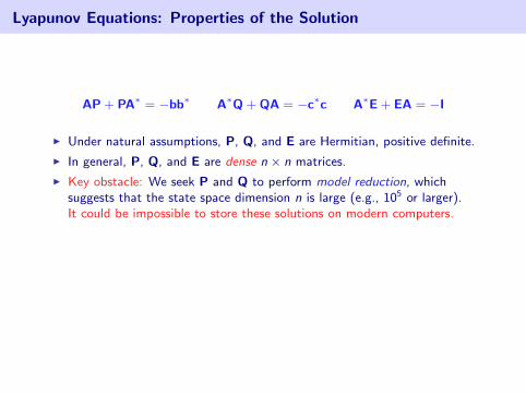
AP + PA∗ = −bb∗ A∗Q + QA = −c∗c A∗E + EA = −I
I Under natural assumptions, P, Q, and E are Hermitian, positive definite.
I In general, P, Q, and E are dense n × n matrices.
I Key obstacle: We seek P and Q to perform model reduction, whichsuggests that the state space dimension n is large (e.g., 105 or larger).It could be impossible to store these solutions on modern computers.
I Penzl [2000] observed, however, that when the right hand side is low rank,the singular values of the solution often decay rapidly.See also [Gudmundsson and Laub 1994].
I Such solutions can be approximated to high accuracy by low-rank matrices.Thus, the approximate solutions can be stored very efficiently.

Lyapunov Equations: Properties of the Solution
AP + PA∗ = −bb∗ A∗Q + QA = −c∗c A∗E + EA = −I
I Under natural assumptions, P, Q, and E are Hermitian, positive definite.
I In general, P, Q, and E are dense n × n matrices.
I Key obstacle: We seek P and Q to perform model reduction, whichsuggests that the state space dimension n is large (e.g., 105 or larger).It could be impossible to store these solutions on modern computers.
I Penzl [2000] observed, however, that when the right hand side is low rank,the singular values of the solution often decay rapidly.See also [Gudmundsson and Laub 1994].
I Such solutions can be approximated to high accuracy by low-rank matrices.Thus, the approximate solutions can be stored very efficiently.
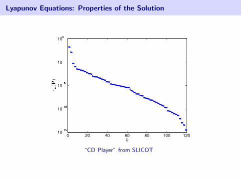
Lyapunov Equations: Properties of the Solution
“CD Player” from SLICOT
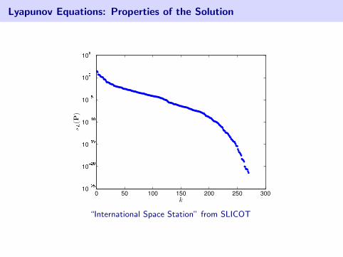
Lyapunov Equations: Properties of the Solution
“International Space Station” from SLICOT

Lyapunov Equations: Properties of the Solution
“Eady” storm track model from SLICOT

Decay of Singular Values of Lyapunov Solutions
The eigenvalues of A affect the rate of decay, as seen in this example.
Normal matrices: A = tridiag(−1, α, 1) with spectrum
σ(A) ⊆ {α + iy : y ∈ [−2, 2]}.
kth
sin
gu
lar
valu
eo
fP
eigenvalues of A
α=
5/
2
α=
1/
2
α = 5/2
α = 1/2
k
Convergence slows as α ↑ 0, i.e., eigenvalues move toward imaginary axis.
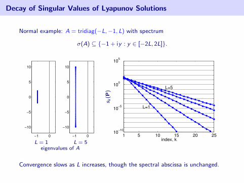
Decay of Singular Values of Lyapunov Solutions
Normal example: A = tridiag(−L,−1, L) with spectrum
σ(A) ⊆ {−1 + iy : y ∈ [−2L, 2L]}.
−1 0
−10
−5
0
5
10
−1 0
−10
−5
0
5
10
1 5 10 15 20 25
10−10
10−5
100
105
L=1
L=5
index, k
s k(P
)
L = 1 L = 5eigenvalues of A
Convergence slows as L increases, though the spectral abscissa is unchanged.
Decay of Singular Values of Lyapunov Solutions
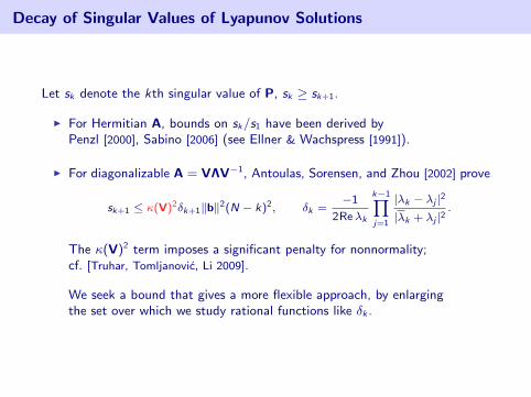
Let sk denote the kth singular value of P, sk ≥ sk+1.
I For Hermitian A, bounds on sk/s1 have been derived byPenzl [2000], Sabino [2006] (see Ellner & Wachspress [1991]).
I For diagonalizable A = VΛV−1, Antoulas, Sorensen, and Zhou [2002] prove
sk+1 ≤ κ(V)2δk+1‖b‖2(N − k)2, δk =−1
2Reλk
k−1Yj=1
|λk − λj |2
|λk + λj |2.
The κ(V)2 term imposes a significant penalty for nonnormality;cf. [Truhar, Tomljanovic, Li 2009].
We seek a bound that gives a more flexible approach, by enlargingthe set over which we study rational functions like δk .

Decay of Singular Values of Lyapunov Solutions
The ADI iteration [Wachspress 1988; Penzl 2000] constructs a rank-kapproximation Pk to P.
I Pick shifts µ1, µ2, . . . , .
I Set
Aµj = (µj − A)(µj + A)−1, bµj =p−2Reµj(µj + A)−1b.
I Set P0 := 0.
I For k = 1, 2, . . . , p
Pk := AµkPk−1A∗µk
+ bµkb∗µk
.
I Then the solution P satisfies
P− Pk = φ(A)Pφ(A)∗,
where rank(Pk) ≤ k and
φ(z) =kY
j=1
µj − z
µj + z.
Decay of Singular Values of Lyapunov Solutions
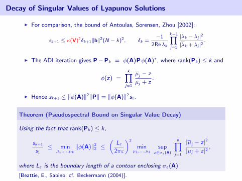
I For comparison, the bound of Antoulas, Sorensen, Zhou [2002]:
sk+1 ≤ κ(V)2δk+1‖b‖2(N − k)2, δk =−1
2Reλk
k−1Yj=1
|λk − λj |2
|λk + λj |2.
I The ADI iteration gives P−Pk = φ(A)Pφ(A)∗, where rank(Pk) ≤ k and
φ(z) =kY
j=1
µj − z
µj + z.
I Hence sk+1 ≤ ‖φ(A)‖2‖P‖ = ‖φ(A)‖2 s1.
Theorem (Pseudospectral Bound on Singular Value Decay)
Using the fact that rank(Pk) ≤ k,
sk+1
s1≤ min
µ1,...,µk
‖φ(A)‖22 ≤
„Lε
2πε
«2
minµ1,...,µk
supz∈σε(A)
kYj=1
|µj − z |2
|µj + z |2 ,
where Lε is the boundary length of a contour enclosing σε(A)
[Beattie, E., Sabino; cf. Beckermann (2004)].
Singular Values of Lyapunov Solutions
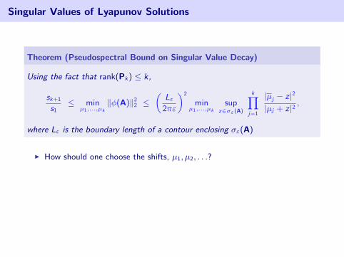
Theorem (Pseudospectral Bound on Singular Value Decay)
Using the fact that rank(Pk) ≤ k,
sk+1
s1≤ min
µ1,...,µk
‖φ(A)‖22 ≤
„Lε
2πε
«2
minµ1,...,µk
supz∈σε(A)
kYj=1
|µj − z |2
|µj + z |2 ,
where Lε is the boundary length of a contour enclosing σε(A)
I How should one choose the shifts, µ1, µ2, . . .?
I One can pick the shifts to minimize the upper bound, i.e., beasymptotically optimal rational interpolation points for σε(A)for some ε > 0.
I Other heuristics are also effective. For example, Sabino [2006] shows thatMATLAB’s fminsearch can give excellent results for a few shifts.

Singular Values of Lyapunov Solutions
Theorem (Pseudospectral Bound on Singular Value Decay)
Using the fact that rank(Pk) ≤ k,
sk+1
s1≤ min
µ1,...,µk
‖φ(A)‖22 ≤
„Lε
2πε
«2
minµ1,...,µk
supz∈σε(A)
kYj=1
|µj − z |2
|µj + z |2 ,
where Lε is the boundary length of a contour enclosing σε(A)
I How should one choose the shifts, µ1, µ2, . . .?
I One can pick the shifts to minimize the upper bound, i.e., beasymptotically optimal rational interpolation points for σε(A)for some ε > 0.
I Other heuristics are also effective. For example, Sabino [2006] shows thatMATLAB’s fminsearch can give excellent results for a few shifts.
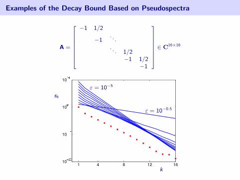
Examples of the Decay Bound Based on Pseudospectra
A =
26666664
−1 1/2
−1. . .
. . . 1/2−1 1/2
−1
37777775 ∈ C16×16
ε = 10−5
ε = 10−0.5
k
sk

Examples of the Decay Bound Based on Pseudospectra
A =
26666664
−1 2
−1. . .
. . . 2−1 2
−1
37777775 ∈ C32×32
−3 −2 −1 0 1
−2
−1
0
1
2
−28
−26
−24
−22
−20
−18
−16
−14
−12
−10
−8
Spectrum, pseudospectra, and numerical range (boundary = dashed line)
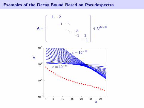
Examples of the Decay Bound Based on Pseudospectra
A =
26666664
−1 2
−1. . .
. . . 2−1 2
−1
37777775 ∈ C32×32
ε = 10−28
ε = 10−10
k
sk
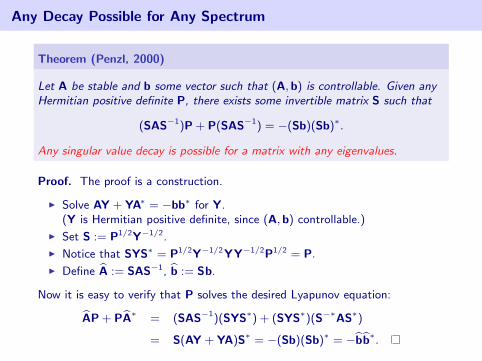
Any Decay Possible for Any Spectrum
Theorem (Penzl, 2000)
Let A be stable and b some vector such that (A, b) is controllable. Given anyHermitian positive definite P, there exists some invertible matrix S such that
(SAS−1)P + P(SAS−1) = −(Sb)(Sb)∗.
Any singular value decay is possible for a matrix with any eigenvalues.
Proof. The proof is a construction.
I Solve AY + YA∗ = −bb∗ for Y.(Y is Hermitian positive definite, since (A, b) controllable.)
I Set S := P1/2Y−1/2.
I Notice that SYS∗ = P1/2Y−1/2 YY−1/2P1/2 = P.
I Define bA := SAS−1, bb := Sb.
Now it is easy to verify that P solves the desired Lyapunov equation:bAP + PbA∗ = (SAS−1)(SYS∗) + (SYS∗)(S−∗AS∗)
= S(AY + YA)S∗ = −(Sb)(Sb)∗ = −bbbb∗.

A Nonnormal Anomaly
The pseudospectral bound and the bound of Antoulas, Sorensen, and Zhouboth predict that the decay rate slows as nonnormality increases.
However, for the solutions to Lyapunov equations this intuition can be wrong[Sabino 2006].
Consider
A =
»−1 α0 −1
–, b =
»t1
–, t ∈ R.
As α grows, A’s departure from normality grows.All bounds suggest that the ‘decay’ rate should worsen as α increases.
The Lyapunov equation AP + PA∗ = −bb∗ has the solution
P =1
4
»2t2 + 2αt + α2 α + 2t
α + 2t 2
–.
For each α, we wish to pick t to maximize the ‘decay’, i.e., s2/s1.This is accomplished for t = −α/2, giving
s2
s1=
α2/4, 0 < α ≤ 2;4/α2, 2 ≤ α.
A Nonnormal Anomaly
The pseudospectral bound and the bound of Antoulas, Sorensen, and Zhouboth predict that the decay rate slows as nonnormality increases.
However, for the solutions to Lyapunov equations this intuition can be wrong[Sabino 2006].
Consider
A =
»−1 α0 −1
–, b =
»t1
–, t ∈ R.
As α grows, A’s departure from normality grows.All bounds suggest that the ‘decay’ rate should worsen as α increases.
The Lyapunov equation AP + PA∗ = −bb∗ has the solution
P =1
4
»2t2 + 2αt + α2 α + 2t
α + 2t 2
–.
For each α, we wish to pick t to maximize the ‘decay’, i.e., s2/s1.
This is accomplished for t = −α/2, giving
s2
s1=
α2/4, 0 < α ≤ 2;4/α2, 2 ≤ α.

A Nonnormal Anomaly
The pseudospectral bound and the bound of Antoulas, Sorensen, and Zhouboth predict that the decay rate slows as nonnormality increases.
However, for the solutions to Lyapunov equations this intuition can be wrong[Sabino 2006].
Consider
A =
»−1 α0 −1
–, b =
»t1
–, t ∈ R.
As α grows, A’s departure from normality grows.All bounds suggest that the ‘decay’ rate should worsen as α increases.
The Lyapunov equation AP + PA∗ = −bb∗ has the solution
P =1
4
»2t2 + 2αt + α2 α + 2t
α + 2t 2
–.
For each α, we wish to pick t to maximize the ‘decay’, i.e., s2/s1.This is accomplished for t = −α/2, giving
s2
s1=
α2/4, 0 < α ≤ 2;4/α2, 2 ≤ α.

Jordan block: 2 × 2 case, numerical illustration
0 1 2 3 4 50
0.25
0.5
0.75
1
wor
st c
ase
ratio
α
Red line:s2
s1=
α2/4, 0 < α ≤ 2;4/α2, 2 ≤ α.
Blue dots: s2/s1 for random b and 2000 α values.
The effect of nonnormality on Lyapunov solutionsremains only partially understood.

Jordan block: 2 × 2 case, numerical illustration
0 1 2 3 4 50
0.25
0.5
0.75
1
wor
st c
ase
ratio
α
Red line:s2
s1=
α2/4, 0 < α ≤ 2;4/α2, 2 ≤ α.
Blue dots: s2/s1 for random b and 2000 α values.
The effect of nonnormality on Lyapunov solutionsremains only partially understood.

4(d) Moment Matching Model Reduction

Krylov methods for moment matching model reduction
We now turn to a model reduction approach where nonnormality plays a crucialrole. Once again, begin with the SISO system
x(t) = Ax(t) + bu(t)
y(t) = cx(t) + du(t),
with A ∈ Cn×n and b, cT ∈ Cn and initial condition x(0) = x0.
Compress the state space to dimension k � n via a projection method:
bx(t) = bAbx(t) + bbu(t)by(t) = bcbx(t) + du(t),
where bA = W∗AV ∈ Ck×k , bb = W∗b ∈ Ck×1, bc = cV ∈ C1×k
for some V,W ∈ Cn×k with W∗V = I.
The matrices V and W are constructed by a Krylov subspace method.

Krylov methods for moment matching model reduction
bA = W∗AV ∈ Ck×k , bb = W∗b ∈ Ck×1, bc = cV ∈ C1×k
Arnoldi Reduction
If V = W and the columns of V span the kth Krylov subspace,
Ran(V) = Kk(A, b) = span{b,Ab, . . . ,Ak−1b},
then the reduced model matches k moments of the system:
bcbAjbb = cAj b, j = 0, . . . , k − 1.
Bi-Lanczos Reduction
If the columns and V and W span the Krylov subspaces
Ran(V) = Kk(A, b) = span{b,Ab, . . . ,Ak−1b}Ran(W) = Kk(A∗, c∗) = span{c∗,A∗c∗, . . . , (A∗)k−1c∗},
then the reduced model matches 2k moments of the system:
bcbAjbb = cAj b, j = 0, . . . , 2k − 1.
Stability of Reduced Order Models
Question
Does the reduced model inherit properties of the original system?
Properties include stability, passivity, second-order structure, etc.
In this lecture we are concerned with stability – and, more generally, thebehavior of eigenvalues of the reduced matrix bA.
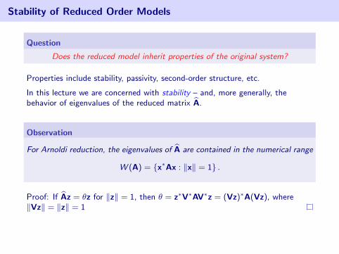
Observation
For Arnoldi reduction, the eigenvalues of bA are contained in the numerical range
W (A) = {x∗Ax : ‖x‖ = 1} .
Proof: If bAz = θz for ‖z‖ = 1, then θ = z∗V∗AV∗z = (Vz)∗A(Vz), where‖Vz‖ = ‖z‖ = 1
No such bound for Bi-Lanczos: the decomposition may not even exist.For the famous ‘CD Player’ model, cb = 0: method breaks down at first step.
Stability of Reduced Order Models
Question
Does the reduced model inherit properties of the original system?
Properties include stability, passivity, second-order structure, etc.
In this lecture we are concerned with stability – and, more generally, thebehavior of eigenvalues of the reduced matrix bA.
Observation
For Arnoldi reduction, the eigenvalues of bA are contained in the numerical range
W (A) = {x∗Ax : ‖x‖ = 1} .
Proof: If bAz = θz for ‖z‖ = 1, then θ = z∗V∗AV∗z = (Vz)∗A(Vz), where‖Vz‖ = ‖z‖ = 1
No such bound for Bi-Lanczos: the decomposition may not even exist.For the famous ‘CD Player’ model, cb = 0: method breaks down at first step.

Stability and Bi-Lanczos
For Bi-Lanczos, the stability question is rather more subtle.
For example, if b and c are nearly orthogonal,the (1,1) entry in bA = W∗AV will generally be very large.
Given a fixed b, one has much freedom to rig poor results via c:
[A]ny three-term recurrence (run for no more than (n +2)/2 steps,where n is the size of the matrix) is the two-sided Lanczos algo-rithm for some left starting vector. [Greenbaum, 1998]

Example: Arnoldi Reduction for Normal versus Nonnormal
The eigenvalues of bA are known as Ritz values.
normal matrix nonnormal matrix
Eigenvalues (•), Ritz values (◦), and numerical range for isospectral matrices.

A Remedy for Unstable Arnoldi Models?
One can counteract instability by restarting the Arnoldi algorithmto shift out unstable eigenvalues [Grimme, Sorensen, Van Dooren, 1994];cf. [Jaimoukha and Kasenally, 1997].
I bA := V∗AV has eigenvalues θ1, . . . , θk (Ritz values for A)
I Suppose θ1, . . . , θp are in the right half plane.
I Replace the starting vector b by the filtered vector
b+ = ψ(A)b, ψ(z) =
pYj=1
(z − θj),
where the filter polynomial ψ “discourages” future Ritz values near theshifts θ1, . . . , θp.
I Build new matrices V, bA with starting vector b+ (implicit restart).
I Now modified moments, b∗ψ(A)∗Ajψ(A)b, will be matched.
Repeat this process until bA has no unstable modes.

Matching the Moments of a Nonnormal Matrix
Model of flutter in a Boeing 767 from SLICOT (n = 55),stabilized by Burke, Lewis, Overton [2003].
−1000 −800 −600 −400 −200 0−600
−400
−200
0
200
400
600
σ(A)
−1 −0.5 0 0.5 1
x 107
−1
−0.8
−0.6
−0.4
−0.2
0
0.2
0.4
0.6
0.8
1x 10
7
W (A)

Matching the Moments of a Nonnormal Matrix
Model of flutter in a Boeing 767 from SLICOT (n = 55),stabilized by Burke, Lewis, Overton [2003].
−100 −50 0 50 100
−100
−50
0
50
100
−6.5
−6
−5.5
−5
−4.5
−4
−3.5
−3
−2.5
−2
σε(A) = {z ∈ C : ‖(z − A)−1‖ > 1/ε}
see [Trefethen & E. 2005]

Reduction via Restarted Arnoldi
10−7
10−5
10−3
10−1
101
103
10−2
100
102
104
106
t
‖x(t
)‖
−100 −50 0 50 100
−100
−50
0
50
100
Transient behavior and spectrum of the original system

Reduction via Restarted Arnoldi
10−7
10−5
10−3
10−1
101
103
10−2
100
102
104
106
t
‖x(t
)‖
−100 −50 0 50 100
−100
−50
0
50
100
Transient behavior and spectrum for reduced system, m = 40

Reduction via Restarted Arnoldi
10−7
10−5
10−3
10−1
101
103
10−2
100
102
104
106
t
‖x(t
)‖
−100 −50 0 50 100
−100
−50
0
50
100
Transient behavior and spectrum for reduced system, m = 40,after one implicit restart

Reduction via Restarted Arnoldi
10−7
10−5
10−3
10−1
101
103
10−2
100
102
104
106
t
‖x(t
)‖
−100 −50 0 50 100
−100
−50
0
50
100
Transient behavior and spectrum for reduced system, m = 40,after two implicit restarts

Reduction via Restarted Arnoldi
10−7
10−5
10−3
10−1
101
103
10−2
100
102
104
106
t
‖x(t
)‖
−100 −50 0 50 100
−100
−50
0
50
100
Transient behavior and spectrum for reduced system, m = 40,after three implicit restarts

Reduction via Restarted Arnoldi
10−7
10−5
10−3
10−1
101
103
10−2
100
102
104
106
t
‖x(t
)‖
−100 −50 0 50 100
−100
−50
0
50
100
Transient behavior and spectrum for reduced system, m = 40,after four implicit restarts
Reduced system is stable, but underestimatestransient growth by several orders of magnitude.

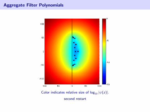
Aggregate Filter Polynomials
Color indicates relative size of log10 |ψ(z)|.
first restart
Aggregate Filter Polynomials
Color indicates relative size of log10 |ψ(z)|.
second restart

Aggregate Filter Polynomials
Color indicates relative size of log10 |ψ(z)|.
third restart
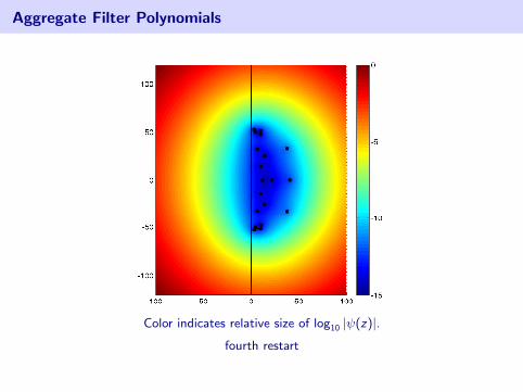
Aggregate Filter Polynomials
Color indicates relative size of log10 |ψ(z)|.
fourth restart
Nonlinear Heat Equation: Revisited
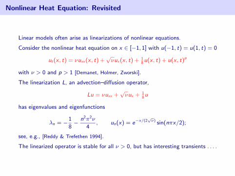
Linear models often arise as linearizations of nonlinear equations.
Consider the nonlinear heat equation on x ∈ [−1, 1] with u(−1, t) = u(1, t) = 0
ut(x , t) = νuxx(x , t) +√νux(x , t) + 1
8u(x , t) + u(x , t)p
with ν > 0 and p > 1 [Demanet, Holmer, Zworski].
The linearization L, an advection–diffusion operator,
Lu = νuxx +√νux + 1
8u
has eigenvalues and eigenfunctions
λn = −1
8− n2π2ν
4, un(x) = e−x/(2
√ν) sin(nπx/2);
see, e.g., [Reddy & Trefethen 1994].
The linearized operator is stable for all ν > 0, but has interesting transients . . . .

Nonnormality in the Linearization
−5 −4 −3 −2 −1 0 1−2.5
−2
−1.5
−1
−0.5
0
0.5
1
1.5
2
2.5
−6
−5
−4
−3
−2
−1
0
Spectrum, pseudospectra, and numerical range (L2 norm, ν = 0.02)
Transient growth can feed the nonlinearitycf. [Trefethen, Trefethen, Reddy, Driscoll 1993], . . . .

Nonnormality in the Linearization
Spectrum, pseudospectra, and numerical range (L2 norm, ν = 0.02)
Transient growth can feed the nonlinearitycf. [Trefethen, Trefethen, Reddy, Driscoll 1993], . . . .

Nonnormality in the Linearization
Spectrum, pseudospectra, and numerical range (L2 norm, ν = 0.02)
Transient growth can feed the nonlinearitycf. [Trefethen, Trefethen, Reddy, Driscoll 1993], . . . .
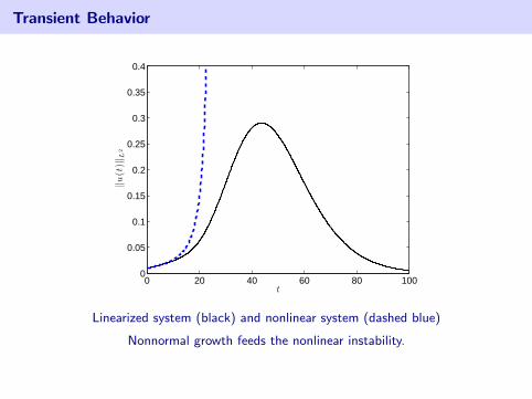
Transient Behavior
0 20 40 60 80 1000
0.05
0.1
0.15
0.2
0.25
0.3
0.35
0.4
t
‖u(t
)‖L
2
Linearized system (black) and nonlinear system (dashed blue)
Nonnormal growth feeds the nonlinear instability.
Red line: estimated “lower bound”: z‖(z − A)−1‖‖u0(t)‖L2 for z = 0.02.

Transient Behavior
Linearized system (black) and nonlinear system (dashed blue)
Nonnormal growth feeds the nonlinear instability.
Red line: estimated “lower bound”: z‖(z − A)−1‖‖u0(t)‖L2 for z = 0.02.

Transient Behavior: Reduction of the Linearized Model
−3 −2.5 −2 −1.5 −1 −0.5 0
x 104
−5
−4
−3
−2
−1
0
1
2
3
4
5
−5 −4 −3 −2 −1 0 1−3
−2
−1
0
1
2
3
entire spectrum zoom
Spectral discretization, n = 128 (black) and Arnoldi reduction, m = 10 (red).
[Many Ritz values capture spurious eigenvalues of the discretization of the left.]

Transient Behavior: Reduction of the Linearized Model
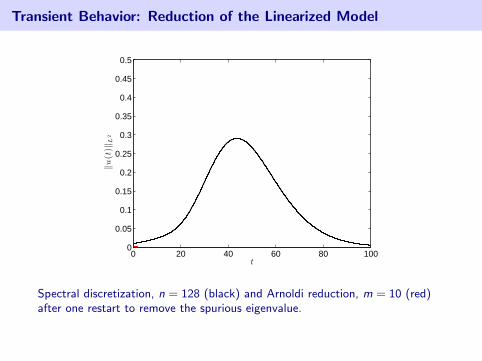
0 20 40 60 80 1000
0.05
0.1
0.15
0.2
0.25
0.3
0.35
0.4
0.45
0.5
t
‖u(t
)‖L
2
Spectral discretization, n = 128 (black) and Arnoldi reduction, m = 10 (red).

Transient Behavior: Reduction of the Linearized Model
−3 −2.5 −2 −1.5 −1 −0.5 0
x 104
−5
−4
−3
−2
−1
0
1
2
3
4
5
−5 −4 −3 −2 −1 0 1−3
−2
−1
0
1
2
3
entire spectrum zoom
Spectral discretization, n = 128 (black) and Arnoldi reduction, m = 10 (red)after a restart to remove the spurious eigenvalue.
[This effectively pushes Ritz values to the left.]
Transient Behavior: Reduction of the Linearized Model
0 20 40 60 80 1000
0.05
0.1
0.15
0.2
0.25
0.3
0.35
0.4
0.45
0.5
t
‖u(t
)‖L
2
Spectral discretization, n = 128 (black) and Arnoldi reduction, m = 10 (red)after one restart to remove the spurious eigenvalue.

Transient Behavior: Reduction of the Linearized Model
0 20 40 60 80 10010
−10
10−8
10−6
10−4
10−2
100
t
‖u(t
)‖L
2
Spectral discretization, n = 128 (black) and Arnoldi reduction, m = 10 (red)after one restart to remove the spurious eigenvalue.

4(c) Nonnormality in Iterative Linear Algebra

Nonnormality and Iterative Linear Algebra
We wish to describe the role of nonnormality in the iterative solution ofdifferential equations.
The GMRES algorithm produces optimal iterates xk whose residualsrk = b− Axk satisfy
‖rk‖ ≤ minp∈Pkp(0)=1
‖p(A)b‖,
where Pk denotes the set of polynomials of degree k or less.
Applying the Cauchy integral theorem bound,
‖rk‖‖b‖ ≤
Lε2πε
minp∈Pkp(0)=1
supz∈σε(A)
|p(z)|.
Different ε values give the best bounds at different stages of convergence.
Illustrations and applications: [Trefethen 1990; E. 2000; Sifuentes, E., Morgan 2011].

GMRES Convergence: Example
Pseudospectral bound for convection–diffusion problem, n = 2304.
ε = 10−3.5, 10−3, 10−3.5, . . . , 10−13
�ε = 10−3.5
-ε =10−13
Bound σε(A) with a circle centered at c, use pk(z) = (1− z/c)k .

Perturbed GMRES and Approximate Preconditioning
I We shall show how psedospectra can be used to bound GMRESconvergence when the coefficient matrix A is slightly perturbed.[Sifuentes, E., Morgan, 2011]
I The primary application result of this work is approximate preconditioning,where we aim to solve Ax = b by the modified system
PAx = Pb
for some invertible P.
I Often one knows an “ideal” preconditioner that is expensive to compute,but for which σ(PA) is easy to analyze. In practice, P is only appliedapproximately. How accurate must it be to provide similar convergence tothe exact preconditioner?
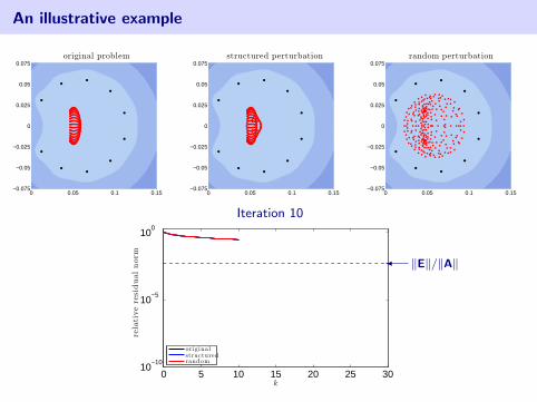
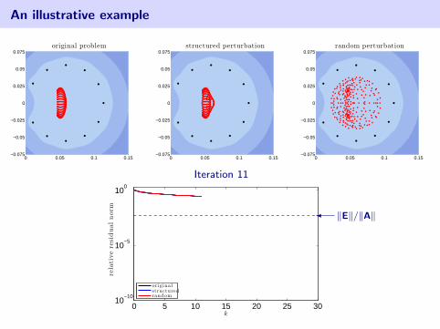
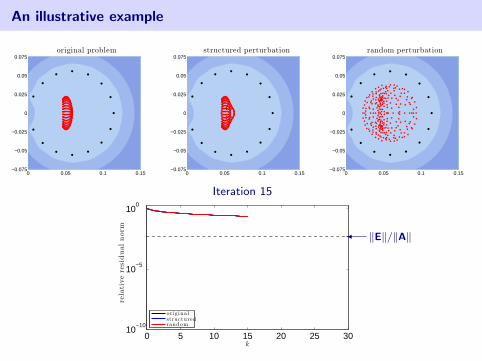
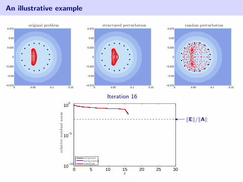
An illustrative example
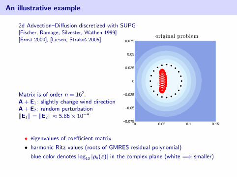
2d Advection–Diffusion discretized with SUPG
0 0.05 0.1 0.15−0.075
−0.05
−0.025
0
0.025
0.05
0.075original problem
[Fischer, Ramage, Silvester, Wathen 1999]
[Ernst 2000], [Liesen, Strakos 2005]
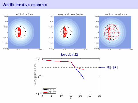
Matrix is of order n = 162.A + E1: slightly change wind directionA + E2: random perturbation‖E1‖ = ‖E2‖ ≈ 5.86× 10⁻⁴
• eigenvalues of coefficient matrix
• harmonic Ritz values (roots of GMRES residual polynomial)
blue color denotes log10 |pk(z)| in the complex plane (white =⇒ smaller)
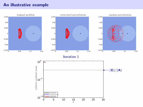
An illustrative example
0 0.05 0.1 0.15−0.075
−0.05
−0.025
0
0.025
0.05
0.075original problem
0 0.05 0.1 0.15−0.075
−0.05
−0.025
0
0.025
0.05
0.075structured perturbation
0 0.05 0.1 0.15−0.075
−0.05
−0.025
0
0.025
0.05
0.075random perturbation
Iteration 1
0 5 10 15 20 25 3010
−10
10−5
100
k
rela
tive
resi
dual
nor
m
originalstructuredrandom
� ‖E‖/‖A‖

An illustrative example
0 0.05 0.1 0.15−0.075
−0.05
−0.025
0
0.025
0.05
0.075original problem
0 0.05 0.1 0.15−0.075
−0.05
−0.025
0
0.025
0.05
0.075structured perturbation
0 0.05 0.1 0.15−0.075
−0.05
−0.025
0
0.025
0.05
0.075random perturbation
Iteration 2
0 5 10 15 20 25 3010
−10
10−5
100
k
rela
tive
resi
dual
nor
m
originalstructuredrandom
� ‖E‖/‖A‖

An illustrative example
0 0.05 0.1 0.15−0.075
−0.05
−0.025
0
0.025
0.05
0.075original problem
0 0.05 0.1 0.15−0.075
−0.05
−0.025
0
0.025
0.05
0.075structured perturbation
0 0.05 0.1 0.15−0.075
−0.05
−0.025
0
0.025
0.05
0.075random perturbation
Iteration 3
0 5 10 15 20 25 3010
−10
10−5
100
k
rela
tive
resi
dual
nor
m
originalstructuredrandom
� ‖E‖/‖A‖
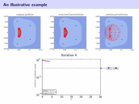
An illustrative example
0 0.05 0.1 0.15−0.075
−0.05
−0.025
0
0.025
0.05
0.075original problem
0 0.05 0.1 0.15−0.075
−0.05
−0.025
0
0.025
0.05
0.075structured perturbation
0 0.05 0.1 0.15−0.075
−0.05
−0.025
0
0.025
0.05
0.075random perturbation
Iteration 4
0 5 10 15 20 25 3010
−10
10−5
100
k
rela
tive
resi
dual
nor
m
originalstructuredrandom
� ‖E‖/‖A‖
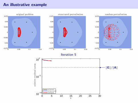
An illustrative example
0 0.05 0.1 0.15−0.075
−0.05
−0.025
0
0.025
0.05
0.075original problem
0 0.05 0.1 0.15−0.075
−0.05
−0.025
0
0.025
0.05
0.075structured perturbation
0 0.05 0.1 0.15−0.075
−0.05
−0.025
0
0.025
0.05
0.075random perturbation
Iteration 5
0 5 10 15 20 25 3010
−10
10−5
100
k
rela
tive
resi
dual
nor
m
originalstructuredrandom
� ‖E‖/‖A‖

An illustrative example
0 0.05 0.1 0.15−0.075
−0.05
−0.025
0
0.025
0.05
0.075original problem
0 0.05 0.1 0.15−0.075
−0.05
−0.025
0
0.025
0.05
0.075structured perturbation
0 0.05 0.1 0.15−0.075
−0.05
−0.025
0
0.025
0.05
0.075random perturbation
Iteration 6
0 5 10 15 20 25 3010
−10
10−5
100
k
rela
tive
resi
dual
nor
m
originalstructuredrandom
� ‖E‖/‖A‖

An illustrative example
0 0.05 0.1 0.15−0.075
−0.05
−0.025
0
0.025
0.05
0.075original problem
0 0.05 0.1 0.15−0.075
−0.05
−0.025
0
0.025
0.05
0.075structured perturbation
0 0.05 0.1 0.15−0.075
−0.05
−0.025
0
0.025
0.05
0.075random perturbation
Iteration 7
0 5 10 15 20 25 3010
−10
10−5
100
k
rela
tive
resi
dual
nor
m
originalstructuredrandom
� ‖E‖/‖A‖

An illustrative example
0 0.05 0.1 0.15−0.075
−0.05
−0.025
0
0.025
0.05
0.075original problem
0 0.05 0.1 0.15−0.075
−0.05
−0.025
0
0.025
0.05
0.075structured perturbation
0 0.05 0.1 0.15−0.075
−0.05
−0.025
0
0.025
0.05
0.075random perturbation
Iteration 8
0 5 10 15 20 25 3010
−10
10−5
100
k
rela
tive
resi
dual
nor
m
originalstructuredrandom
� ‖E‖/‖A‖
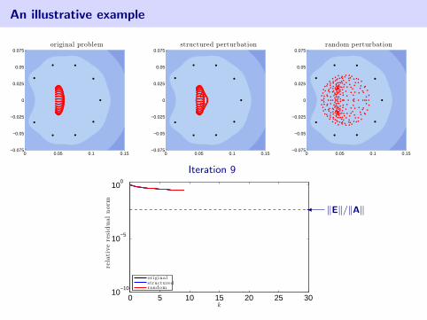
An illustrative example
0 0.05 0.1 0.15−0.075
−0.05
−0.025
0
0.025
0.05
0.075original problem
0 0.05 0.1 0.15−0.075
−0.05
−0.025
0
0.025
0.05
0.075structured perturbation
0 0.05 0.1 0.15−0.075
−0.05
−0.025
0
0.025
0.05
0.075random perturbation
Iteration 9
0 5 10 15 20 25 3010
−10
10−5
100
k
rela
tive
resi
dual
nor
m
originalstructuredrandom
� ‖E‖/‖A‖
An illustrative example
0 0.05 0.1 0.15−0.075
−0.05
−0.025
0
0.025
0.05
0.075original problem
0 0.05 0.1 0.15−0.075
−0.05
−0.025
0
0.025
0.05
0.075structured perturbation
0 0.05 0.1 0.15−0.075
−0.05
−0.025
0
0.025
0.05
0.075random perturbation
Iteration 10
0 5 10 15 20 25 3010
−10
10−5
100
k
rela
tive
resi
dual
nor
m
originalstructuredrandom
� ‖E‖/‖A‖
An illustrative example
0 0.05 0.1 0.15−0.075
−0.05
−0.025
0
0.025
0.05
0.075original problem
0 0.05 0.1 0.15−0.075
−0.05
−0.025
0
0.025
0.05
0.075structured perturbation
0 0.05 0.1 0.15−0.075
−0.05
−0.025
0
0.025
0.05
0.075random perturbation
Iteration 11
0 5 10 15 20 25 3010
−10
10−5
100
k
rela
tive
resi
dual
nor
m
originalstructuredrandom
� ‖E‖/‖A‖

An illustrative example
0 0.05 0.1 0.15−0.075
−0.05
−0.025
0
0.025
0.05
0.075original problem
0 0.05 0.1 0.15−0.075
−0.05
−0.025
0
0.025
0.05
0.075structured perturbation
0 0.05 0.1 0.15−0.075
−0.05
−0.025
0
0.025
0.05
0.075random perturbation
Iteration 12
0 5 10 15 20 25 3010
−10
10−5
100
k
rela
tive
resi
dual
nor
m
originalstructuredrandom
� ‖E‖/‖A‖

An illustrative example
0 0.05 0.1 0.15−0.075
−0.05
−0.025
0
0.025
0.05
0.075original problem
0 0.05 0.1 0.15−0.075
−0.05
−0.025
0
0.025
0.05
0.075structured perturbation
0 0.05 0.1 0.15−0.075
−0.05
−0.025
0
0.025
0.05
0.075random perturbation
Iteration 13
0 5 10 15 20 25 3010
−10
10−5
100
k
rela
tive
resi
dual
nor
m
originalstructuredrandom
� ‖E‖/‖A‖

An illustrative example
0 0.05 0.1 0.15−0.075
−0.05
−0.025
0
0.025
0.05
0.075original problem
0 0.05 0.1 0.15−0.075
−0.05
−0.025
0
0.025
0.05
0.075structured perturbation
0 0.05 0.1 0.15−0.075
−0.05
−0.025
0
0.025
0.05
0.075random perturbation
Iteration 14
0 5 10 15 20 25 3010
−10
10−5
100
k
rela
tive
resi
dual
nor
m
originalstructuredrandom
� ‖E‖/‖A‖
An illustrative example
0 0.05 0.1 0.15−0.075
−0.05
−0.025
0
0.025
0.05
0.075original problem
0 0.05 0.1 0.15−0.075
−0.05
−0.025
0
0.025
0.05
0.075structured perturbation
0 0.05 0.1 0.15−0.075
−0.05
−0.025
0
0.025
0.05
0.075random perturbation
Iteration 15
0 5 10 15 20 25 3010
−10
10−5
100
k
rela
tive
resi
dual
nor
m
originalstructuredrandom
� ‖E‖/‖A‖
An illustrative example
0 0.05 0.1 0.15−0.075
−0.05
−0.025
0
0.025
0.05
0.075original problem
0 0.05 0.1 0.15−0.075
−0.05
−0.025
0
0.025
0.05
0.075structured perturbation
0 0.05 0.1 0.15−0.075
−0.05
−0.025
0
0.025
0.05
0.075random perturbation
Iteration 16
0 5 10 15 20 25 3010
−10
10−5
100
k
rela
tive
resi
dual
nor
m
originalstructuredrandom
� ‖E‖/‖A‖

An illustrative example
0 0.05 0.1 0.15−0.075
−0.05
−0.025
0
0.025
0.05
0.075original problem
0 0.05 0.1 0.15−0.075
−0.05
−0.025
0
0.025
0.05
0.075structured perturbation
0 0.05 0.1 0.15−0.075
−0.05
−0.025
0
0.025
0.05
0.075random perturbation
Iteration 17
0 5 10 15 20 25 3010
−10
10−5
100
k
rela
tive
resi
dual
nor
m
originalstructuredrandom
� ‖E‖/‖A‖

An illustrative example
0 0.05 0.1 0.15−0.075
−0.05
−0.025
0
0.025
0.05
0.075original problem
0 0.05 0.1 0.15−0.075
−0.05
−0.025
0
0.025
0.05
0.075structured perturbation
0 0.05 0.1 0.15−0.075
−0.05
−0.025
0
0.025
0.05
0.075random perturbation
Iteration 18
0 5 10 15 20 25 3010
−10
10−5
100
k
rela
tive
resi
dual
nor
m
originalstructuredrandom
� ‖E‖/‖A‖

An illustrative example
0 0.05 0.1 0.15−0.075
−0.05
−0.025
0
0.025
0.05
0.075original problem
0 0.05 0.1 0.15−0.075
−0.05
−0.025
0
0.025
0.05
0.075structured perturbation
0 0.05 0.1 0.15−0.075
−0.05
−0.025
0
0.025
0.05
0.075random perturbation
Iteration 19
0 5 10 15 20 25 3010
−10
10−5
100
k
rela
tive
resi
dual
nor
m
originalstructuredrandom
� ‖E‖/‖A‖

An illustrative example
0 0.05 0.1 0.15−0.075
−0.05
−0.025
0
0.025
0.05
0.075original problem
0 0.05 0.1 0.15−0.075
−0.05
−0.025
0
0.025
0.05
0.075structured perturbation
0 0.05 0.1 0.15−0.075
−0.05
−0.025
0
0.025
0.05
0.075random perturbation
Iteration 20
0 5 10 15 20 25 3010
−10
10−5
100
k
rela
tive
resi
dual
nor
m
originalstructuredrandom
� ‖E‖/‖A‖

An illustrative example
0 0.05 0.1 0.15−0.075
−0.05
−0.025
0
0.025
0.05
0.075original problem
0 0.05 0.1 0.15−0.075
−0.05
−0.025
0
0.025
0.05
0.075structured perturbation
0 0.05 0.1 0.15−0.075
−0.05
−0.025
0
0.025
0.05
0.075random perturbation
Iteration 21
0 5 10 15 20 25 3010
−10
10−5
100
k
rela
tive
resi
dual
nor
m
originalstructuredrandom
� ‖E‖/‖A‖
An illustrative example
0 0.05 0.1 0.15−0.075
−0.05
−0.025
0
0.025
0.05
0.075original problem
0 0.05 0.1 0.15−0.075
−0.05
−0.025
0
0.025
0.05
0.075structured perturbation
0 0.05 0.1 0.15−0.075
−0.05
−0.025
0
0.025
0.05
0.075random perturbation
Iteration 22
0 5 10 15 20 25 3010
−10
10−5
100
k
rela
tive
resi
dual
nor
m
originalstructuredrandom
� ‖E‖/‖A‖

An illustrative example
0 0.05 0.1 0.15−0.075
−0.05
−0.025
0
0.025
0.05
0.075original problem
0 0.05 0.1 0.15−0.075
−0.05
−0.025
0
0.025
0.05
0.075structured perturbation
0 0.05 0.1 0.15−0.075
−0.05
−0.025
0
0.025
0.05
0.075random perturbation
Iteration 23
0 5 10 15 20 25 3010
−10
10−5
100
k
rela
tive
resi
dual
nor
m
originalstructuredrandom
� ‖E‖/‖A‖
An illustrative example
0 0.05 0.1 0.15−0.075
−0.05
−0.025
0
0.025
0.05
0.075original problem
0 0.05 0.1 0.15−0.075
−0.05
−0.025
0
0.025
0.05
0.075structured perturbation
0 0.05 0.1 0.15−0.075
−0.05
−0.025
0
0.025
0.05
0.075random perturbation
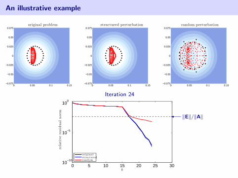
Iteration 24
0 5 10 15 20 25 3010
−10
10−5
100
k
rela
tive
resi
dual
nor
m
originalstructuredrandom
� ‖E‖/‖A‖

An illustrative example
0 0.05 0.1 0.15−0.075
−0.05
−0.025
0
0.025
0.05
0.075original problem
0 0.05 0.1 0.15−0.075
−0.05
−0.025
0
0.025
0.05
0.075structured perturbation
0 0.05 0.1 0.15−0.075
−0.05
−0.025
0
0.025
0.05
0.075random perturbation
Iteration 25
0 5 10 15 20 25 3010
−10
10−5
100
k
rela
tive
resi
dual
nor
m
originalstructuredrandom
� ‖E‖/‖A‖

An illustrative example
0 0.05 0.1 0.15−0.075
−0.05
−0.025
0
0.025
0.05
0.075original problem
0 0.05 0.1 0.15−0.075
−0.05
−0.025
0
0.025
0.05
0.075structured perturbation
0 0.05 0.1 0.15−0.075
−0.05
−0.025
0
0.025
0.05
0.075random perturbation
Iteration 26
0 5 10 15 20 25 3010
−10
10−5
100
k
rela
tive
resi
dual
nor
m
originalstructuredrandom
� ‖E‖/‖A‖

An illustrative example
0 0.05 0.1 0.15−0.075
−0.05
−0.025
0
0.025
0.05
0.075original problem
0 0.05 0.1 0.15−0.075
−0.05
−0.025
0
0.025
0.05
0.075structured perturbation
0 0.05 0.1 0.15−0.075
−0.05
−0.025
0
0.025
0.05
0.075random perturbation
Iteration 27
0 5 10 15 20 25 3010
−10
10−5
100
k
rela
tive
resi
dual
nor
m
originalstructuredrandom
� ‖E‖/‖A‖

An illustrative example
0 0.05 0.1 0.15−0.075
−0.05
−0.025
0
0.025
0.05
0.075original problem
0 0.05 0.1 0.15−0.075
−0.05
−0.025
0
0.025
0.05
0.075structured perturbation
0 0.05 0.1 0.15−0.075
−0.05
−0.025
0
0.025
0.05
0.075random perturbation
Iteration 28
0 5 10 15 20 25 3010
−10
10−5
100
k
rela
tive
resi
dual
nor
m
originalstructuredrandom
� ‖E‖/‖A‖

An illustrative example
0 0.05 0.1 0.15−0.075
−0.05
−0.025
0
0.025
0.05
0.075original problem
0 0.05 0.1 0.15−0.075
−0.05
−0.025
0
0.025
0.05
0.075structured perturbation
0 0.05 0.1 0.15−0.075
−0.05
−0.025
0
0.025
0.05
0.075random perturbation
Iteration 29
0 5 10 15 20 25 3010
−10
10−5
100
k
rela
tive
resi
dual
nor
m
originalstructuredrandom
� ‖E‖/‖A‖

An illustrative example
0 0.05 0.1 0.15−0.075
−0.05
−0.025
0
0.025
0.05
0.075original problem
0 0.05 0.1 0.15−0.075
−0.05
−0.025
0
0.025
0.05
0.075structured perturbation
0 0.05 0.1 0.15−0.075
−0.05
−0.025
0
0.025
0.05
0.075random perturbation
Iteration 30
0 5 10 15 20 25 3010
−10
10−5
100
k
rela
tive
resi
dual
nor
m
originalstructuredrandom
� ‖E‖/‖A‖

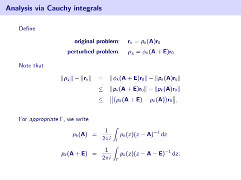
Analysis via Cauchy integrals
Define
original problem: rk = pk(A)r0
perturbed problem: ρk = φk(A + E)r0
Note that
‖ρk‖ − ‖rk‖ = ‖φk(A + E)r0‖ − ‖pk(A)r0‖
≤ ‖pk(A + E)r0‖ − ‖pk(A)r0‖
≤‚‚`pk(A + E)− pk(A)
´r0
‚‚.
For appropriate Γ, we write
pk(A) =1
2πi
ZΓ
pk(z)(z − A)−1 dz
pk(A + E) =1
2πi
ZΓ
pk(z)(z − A− E)−1 dz .
Analysis via Cauchy integrals
Define
original problem: rk = pk(A)r0
perturbed problem: ρk = φk(A + E)r0
Note that
‖ρk‖ − ‖rk‖ = ‖φk(A + E)r0‖ − ‖pk(A)r0‖
≤ ‖pk(A + E)r0‖ − ‖pk(A)r0‖
≤‚‚`pk(A + E)− pk(A)
´r0
‚‚.For appropriate Γ, we write
pk(A) =1
2πi
ZΓ
pk(z)(z − A)−1 dz
pk(A + E) =1
2πi
ZΓ
pk(z)(z − A− E)−1 dz .

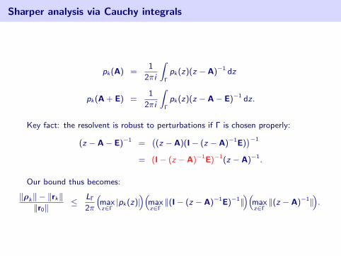
Sharper analysis via Cauchy integrals
pk(A) =1
2πi
ZΓ
pk(z)(z − A)−1 dz
pk(A + E) =1
2πi
ZΓ
pk(z)(z − A− E)−1 dz .
Key fact: the resolvent is robust to perturbations if Γ is chosen properly:
(z − A− E)−1 =`(z − A)(I− (z − A)−1E)
´−1
= (I− (z − A)−1E)−1(z − A)−1.
Our bound thus becomes:
‖ρk‖ − ‖rk‖‖r0‖
≤ LΓ
2π
“maxz∈Γ|pk(z)|
”“maxz∈Γ‖(I− (z − A)−1E)−1‖
”“maxz∈Γ‖(z − A)−1‖
”.
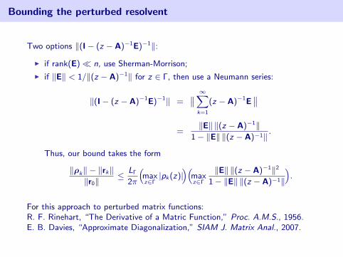
Bounding the perturbed resolvent
Two options ‖(I− (z − A)−1E)−1‖:
I if rank(E)� n, use Sherman-Morrison;
I if ‖E‖ < 1/‖(z − A)−1‖ for z ∈ Γ, then use a Neumann series:
‖(I− (z − A)−1E)−1‖ =‚‚ ∞X
k=1
(z − A)−1E‚‚
=‖E‖ ‖(z − A)−1‖
1− ‖E‖ ‖(z − A)−1‖ .
Thus, our bound takes the form
‖ρk‖ − ‖rk‖‖r0‖
≤ LΓ
2π
“maxz∈Γ|pk(z)|
”“maxz∈Γ
‖E‖ ‖(z − A)−1‖2
1− ‖E‖ ‖(z − A)−1‖
”.
For this approach to perturbed matrix functions:R. F. Rinehart, “The Derivative of a Matric Function,” Proc. A.M.S., 1956.E. B. Davies, “Approximate Diagonalization,” SIAM J. Matrix Anal., 2007.

How to select the contour Γ ?
‖ρk‖ − ‖rk‖‖r0‖
≤ LΓ
2π
“maxz∈Γ|pk(z)|
”“maxz∈Γ
‖E‖ ‖(z − A)−1‖2
1− ‖E‖ ‖(z − A)−1‖
”.
We have competing goals that affect the selection of Γ:
I Γ should be close enough to the spectrum of A that |pk(z)| is small;
I Γ should be far enough from the spectrum of A that ‖(z − A)−1‖ is small.

How to select the contour Γ ?
‖ρk‖ − ‖rk‖‖r0‖
≤ LΓ
2π
“maxz∈Γ|pk(z)|
”“maxz∈Γ
‖E‖ ‖(z − A)−1‖2
1− ‖E‖ ‖(z − A)−1‖
”.
Take Γ to be the boundary of the δ-pseudospectrum, σδ(A).
0 0.05 0.1 0.15−0.075
−0.05
−0.025
0
0.025
0.05
0.075
level sets of ‖(z − A)−1‖σδ(A), δ = 10−2.5, 10−3.5, . . . , 10−7.5
level sets of |p18(z)||p18(z)| = 100, 10−1, . . . , 10−5
0 0.05 0.1 0.15−0.075
−0.05
−0.025
0
0.025
0.05
0.075
cf. [Trefethen 1990; Toh & Trefethen 1998]
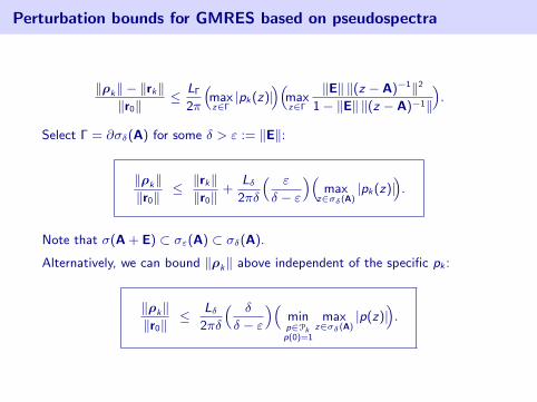
Perturbation bounds for GMRES based on pseudospectra
‖ρk‖ − ‖rk‖‖r0‖
≤ LΓ
2π
“maxz∈Γ|pk(z)|
”“maxz∈Γ
‖E‖ ‖(z − A)−1‖2
1− ‖E‖ ‖(z − A)−1‖
”.
Select Γ = ∂σδ(A) for some δ > ε := ‖E‖:
‖ρk‖‖r0‖
≤ ‖rk‖‖r0‖
+Lδ
2πδ
“ ε
δ − ε
”“max
z∈σδ(A)|pk(z)|
”.
Note that σ(A + E) ⊂ σε(A) ⊂ σδ(A).
Alternatively, we can bound ‖ρk‖ above independent of the specific pk :
‖ρk‖‖r0‖
≤ Lδ2πδ
“ δ
δ − ε
”“minp∈Pkp(0)=1
maxz∈σδ(A)
|p(z)|”.

Example: SUPG Matrix for N = 32, ν = 0.01
N = 32, ν = 0.01 =⇒ A ∈ R1024×1024.
perturbation size: ‖E‖ = 10−4‖A‖
original GMRES residual curve for Ax = b
perturbed GMRES residual curve for (A + E)x = b
upper bound on perturbed residual(δ = 10−5.2, 10−5, 10−4.5, . . . , 10−3, 10−2.9)

Example: SUPG Matrix for N = 32, ν = 0.01
N = 32, ν = 0.01 =⇒ A ∈ R1024×1024.
perturbation size: ‖E‖ = 10−6‖A‖
original GMRES residual curve for Ax = b
perturbed GMRES residual curve for (A + E)x = b
upper bound on perturbed residual(δ = 10−7.2, 10−7, 10−6.5, . . . , 10−3, 10−2.9)

Example: SUPG Matrix for N = 32, ν = 0.01
N = 32, ν = 0.01 =⇒ A ∈ R1024×1024.
perturbation size: ‖E‖ = 10−8‖A‖
original GMRES residual curve for Ax = b
perturbed GMRES residual curve for (A + E)x = b
upper bound on perturbed residual(δ = 10−9.2, 10−9, 10−8.5, . . . , 10−3, 10−2.9)
Nonnormality in Eigenvalue Computations
Here we shall only consider the simplest iterative method for computingeigenvalues: the power method.
Given a starting vector x0, repeatedly apply A:
xk = Akx0.
Assume A is diagonalizable,
A =nX
j=1
λjvjbv∗jwith eigenvalues
|λ1| > |λ2| ≥ · · · ≥ |λn|.Then if x0 =
Pγjvj , then
xk = Akx0 =nX
j=1
λkj vj .
Hence if γ1 6= 0, as k →∞∠(xk , v1)→ 0
at the asymptotic rate |λ2|/|/|λ1|.

Transient Behavior of the Power Method
Large coefficients in the expansion of x0 in the eigenvector basis can lead tocancellation effects in xk = Akx0.
Example: here different choices of α and β affect eigenvalue conditioning,
A =
241 α 00 3/4 β0 0 −3/4
35 , v1 =
24100
35 , v2 =
24−4α10
35 , v3 =
248αβ/21−2β/3
1
35 .
:v1
6v3
}v2
x0x2
x4x6
x8
x1
x3x5
x7 :v2:v1
6v3
x0
x1, ..., x8 :v1
iv3
kv2
x0x2
x4x6
x8x1
x3 x5 x7
normal nonnormal nonnormalv1 ⊥ v2 ⊥ v3 v1 6⊥ v2 ⊥ v3 v1 ⊥ v2 6⊥ v3
α = β = 0 α = 10, β = 0 α = 0, β = 10
Cf. [Beattie, E., Rossi 2004; Beattie, E., Sorensen 2005]

4(d) Pseudospectra of Operators

Pseudospectra with More General Norms
Recall our definition of pseudospectra of a matrix from Lecture 1.
Definition (ε-pseudospectrum)
For any ε > 0, the ε-pseudospectrum of A, denoted σε(A), is the set
σε(A) = {z ∈ C : z ∈ σ(A + E) for some E ∈ Cn×n with ‖E‖ < ε}.
At the time, we assumed that ‖ · ‖ was the vector 2-norm on Cn and the“operator norm” it induces,
‖A‖ = sup‖x‖=1
‖Ax‖.
Now we address various generalizations:
I More general induced/operator norms on Cn;
I Matrix norms on Cn×n not induced by vector norms;
I Infinite dimensional Banach or Hilbert spaces, with the operator norm.
In applications, the use of the proper norm is an essential (but sometimesoverlooked) aspect of pseudospectral theory.

Equivalent definitions in the induced 2-norm
Suppose for the moment that we still use the vector 2-norm, ‖x‖ =√
x∗x.
In our discussion (especially about computing pseudospectra) we haveoccasionally used the fact that
‖(z − A)−1‖ =1
smin(z − A).
Theorem
The following four definitions of the ε-pseudospectrum are equivalent:
1. σε(A) = {z ∈ C : z ∈ σ(A + E) for some E ∈ C n×n with ‖E‖ < ε};2. σε(A) = {z ∈ C : ‖(z − A)−1‖ > 1/ε};
2a. σε(A) = {z ∈ C : smin(z − A) < ε};3. σε(A) = {z ∈ C : ‖Av − zv‖ < ε for some unit vector v ∈ C n}.
This equivalence (2)=(2a) is a property of the vector 2-norm that can beextended to any norm induced by an inner product, 〈x, y〉 := yTGx for
G Hermitian positive definite; the adjoint becomes A? = G−1AT
G.

Pseudospectra with Induced Norms on Cn
Let ‖ · ‖ denote any vector norm on Cn and let
‖A‖ = sup‖x‖=1
‖Ax‖.
The equivalence of the three definitions of the ε-pseudospectrum still hold, butone proof gets generalized.
Theorem
The following three definitions of the ε-pseudospectrum are equivalent:
1. σε(A) = {z ∈ C : z ∈ σ(A + E) for some E ∈ C n×n with ‖E‖ < ε};2. σε(A) = {z ∈ C : ‖(z − A)−1‖ > 1/ε};3. σε(A) = {z ∈ C : ‖Av − zv‖ < ε for some unit vector v ∈ C n}.
Proof. (3) =⇒ (1)
Given a unit vector v such that ‖Av − zv‖ < ε, define r := Av − zv.Now set E := −rw∗, where w is a vector such that w∗v = 1(possible by the theory of dual norms, or Hahn–Banach), so that
(A + E)v = (A− rw∗)v = Av − r = zv.
Hence z ∈ σ(A + E).

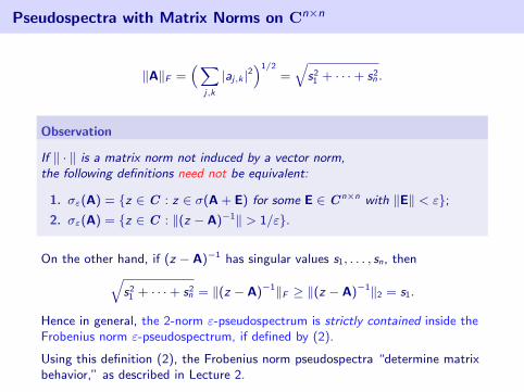
Pseudospectra with Matrix Norms on Cn×n
We can define pseudospectra for a matrix norm that is not induced by a vectornorm, such as the Frobenius norm (a.k.a. Schatten 2-norm):
‖A‖F =“X
j,k
|aj,k |2”1/2
=q
s21 + · · ·+ s2
n .
Observation
If ‖ · ‖ is a matrix norm not induced by a vector norm,the following definitions need not be equivalent:
1. σε(A) = {z ∈ C : z ∈ σ(A + E) for some E ∈ C n×n with ‖E‖ < ε};2. σε(A) = {z ∈ C : ‖(z − A)−1‖ > 1/ε}.

Pseudospectra with Matrix Norms on Cn×n
‖A‖F =“X
j,k
|aj,k |2”1/2
=q
s21 + · · ·+ s2
n .
Observation
If ‖ · ‖ is a matrix norm not induced by a vector norm,the following definitions need not be equivalent:
1. σε(A) = {z ∈ C : z ∈ σ(A + E) for some E ∈ C n×n with ‖E‖ < ε};2. σε(A) = {z ∈ C : ‖(z − A)−1‖ > 1/ε}.
Let (s, u, v) be the smallest singular value and corresponding singular vectorsfor z − A, so that (z − A)v = su. Define E = −suv∗, so that
(A + E)v = (A + suv∗)v = Av + su = zv,
so z ∈ σ(A + E). Notice that ‖E‖F = ‖E‖2 = s.
Since ‖E‖F ≥ ‖E‖2 for all E, we conclude that the 2-norm and Frobenius-normpseudospectra are identical, by definition (1).
Pseudospectra with Matrix Norms on Cn×n
‖A‖F =“X
j,k
|aj,k |2”1/2
=q
s21 + · · ·+ s2
n .
Observation
If ‖ · ‖ is a matrix norm not induced by a vector norm,the following definitions need not be equivalent:
1. σε(A) = {z ∈ C : z ∈ σ(A + E) for some E ∈ C n×n with ‖E‖ < ε};2. σε(A) = {z ∈ C : ‖(z − A)−1‖ > 1/ε}.
On the other hand, if (z − A)−1 has singular values s1, . . . , sn, thenqs2
1 + · · ·+ s2n = ‖(z − A)−1‖F ≥ ‖(z − A)−1‖2 = s1.
Hence in general, the 2-norm ε-pseudospectrum is strictly contained inside theFrobenius norm ε-pseudospectrum, if defined by (2).
Using this definition (2), the Frobenius norm pseudospectra “determine matrixbehavior,” as described in Lecture 2.

Computation of Pseudospectra in General Norms
When describing computation of σε(A), our algorithms (and EigTool) used the2-norm. Different norms require further consideration.
I Norm induced by 〈x, y〉 := y∗Gx.Factor G = R∗R (e.g., Cholesky decomposition, matrix square root).Then for any matrix A ∈ Cn×n,
‖A‖2 = supx6=0
‖Ax‖2
‖x‖2= sup
x 6=0
x∗A∗GAx
x∗Gx
= supx 6=0
x∗R∗R−∗A∗R∗RAR−1Rx
x∗R∗Rx
= supy=Rxx 6=0
y(R−∗A∗R∗)(RAR−1)y
y∗y= ‖RAR−1‖2
2.
Hence, the G-norm pseudospectra of A are the same as the 2-normpseudospectra of RAR−1. This permits the use of EigTool withoutmodification: just call eigtool(R*A/R).
I To compute pseudospectra in other norms, one typically needs toexplicitly compute (z − A)−1 at each point on a computational grid.
Pseudospectra in Infinite Dimensional Spaces
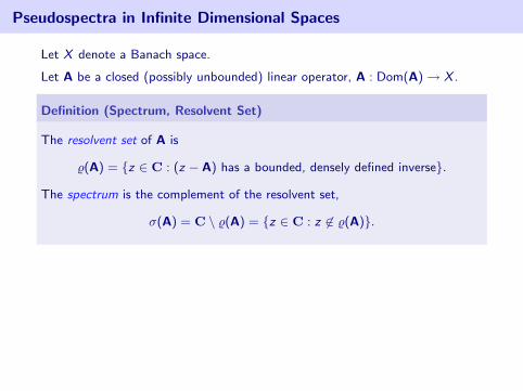
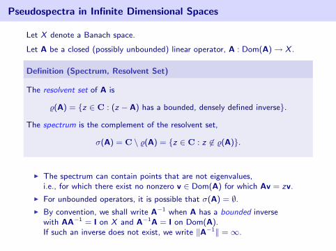
Let X denote a Banach space.
Let A be a closed (possibly unbounded) linear operator, A : Dom(A)→ X .
Definition (Spectrum, Resolvent Set)
The resolvent set of A is
%(A) = {z ∈ C : (z − A) has a bounded, densely defined inverse}.
The spectrum is the complement of the resolvent set,
σ(A) = C \ %(A) = {z ∈ C : z 6∈ %(A)}.
I The spectrum can contain points that are not eigenvalues,i.e., for which there exist no nonzero v ∈ Dom(A) for which Av = zv.
I For unbounded operators, it is possible that σ(A) = ∅.I By convention, we shall write A−1 when A has a bounded inverse
with AA−1 = I on X and A−1A = I on Dom(A).If such an inverse does not exist, we write ‖A−1‖ =∞.
Pseudospectra in Infinite Dimensional Spaces
Let X denote a Banach space.
Let A be a closed (possibly unbounded) linear operator, A : Dom(A)→ X .
Definition (Spectrum, Resolvent Set)
The resolvent set of A is
%(A) = {z ∈ C : (z − A) has a bounded, densely defined inverse}.
The spectrum is the complement of the resolvent set,
σ(A) = C \ %(A) = {z ∈ C : z 6∈ %(A)}.
I The spectrum can contain points that are not eigenvalues,i.e., for which there exist no nonzero v ∈ Dom(A) for which Av = zv.
I For unbounded operators, it is possible that σ(A) = ∅.I By convention, we shall write A−1 when A has a bounded inverse
with AA−1 = I on X and A−1A = I on Dom(A).If such an inverse does not exist, we write ‖A−1‖ =∞.
Pseudospectra
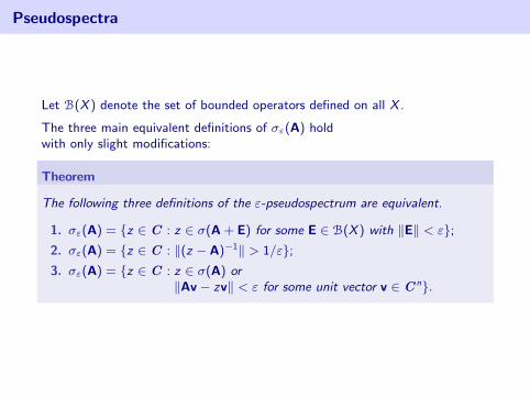
Let B(X ) denote the set of bounded operators defined on all X .
The three main equivalent definitions of σε(A) holdwith only slight modifications:
Theorem
The following three definitions of the ε-pseudospectrum are equivalent.
1. σε(A) = {z ∈ C : z ∈ σ(A + E) for some E ∈ B(X ) with ‖E‖ < ε};2. σε(A) = {z ∈ C : ‖(z − A)−1‖ > 1/ε};3. σε(A) = {z ∈ C : z ∈ σ(A) or
‖Av − zv‖ < ε for some unit vector v ∈ C n}.
Stability of Bounded Invertibility
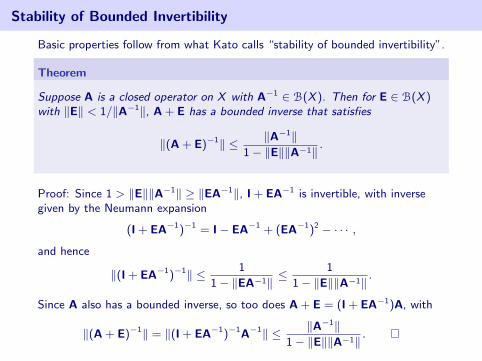
Basic properties follow from what Kato calls “stability of bounded invertibility”.
Theorem
Suppose A is a closed operator on X with A−1 ∈ B(X ). Then for E ∈ B(X )with ‖E‖ < 1/‖A−1‖, A + E has a bounded inverse that satisfies
‖(A + E)−1‖ ≤ ‖A−1‖1− ‖E‖‖A−1‖ .
Proof: Since 1 > ‖E‖‖A−1‖ ≥ ‖EA−1‖, I + EA−1 is invertible, with inversegiven by the Neumann expansion
(I + EA−1)−1 = I− EA−1 + (EA−1)2 − · · · ,
and hence
‖(I + EA−1)−1‖ ≤ 1
1− ‖EA−1‖ ≤1
1− ‖E‖‖A−1‖ .
Since A also has a bounded inverse, so too does A + E = (I + EA−1)A, with
‖(A + E)−1‖ = ‖(I + EA−1)−1A−1‖ ≤ ‖A−1‖1− ‖E‖‖A−1‖ .

Basic Properties of Pseudospectra on Banach Spaces
I ‖(z − A)−1‖ ≥ 1/dist(z , σ(A)).
I (z − A)−1 is analytic on %(A).
I ‖(z − A)−1‖ is an unbounded, subharmonic function on %(A).
I For all ε > 0, σε(A) is a nonempty open subset of C.
I Each bounded component of σε(A) intersects σ(A).
Weak versus Strong Inequalities
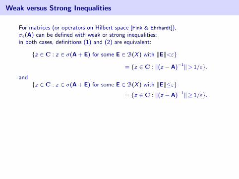
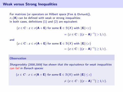
For matrices (or operators on Hilbert space [Fink & Ehrhardt]),σε(A) can be defined with weak or strong inequalities:in both cases, definitions (1) and (2) are equivalent:
{z ∈ C : z ∈ σ(A + E) for some E ∈ B(X ) with ‖E‖<ε}
= {z ∈ C : ‖(z − A)−1‖> 1/ε}.
and{z ∈ C : z ∈ σ(A + E) for some E ∈ B(X ) with ‖E‖≤ε}
= {z ∈ C : ‖(z − A)−1‖≥ 1/ε}.
Observation
Shargorodsky [2008,2009] has shown that the equivalence for weak inequalitiescan fail in Banach spaces:
{z ∈ C : z ∈ σ(A + E) for some E ∈ B(X ) with ‖E‖≤ ε}
6= {z ∈ C : ‖(z − A)−1‖≥ 1/ε}.
Weak versus Strong Inequalities
For matrices (or operators on Hilbert space [Fink & Ehrhardt]),σε(A) can be defined with weak or strong inequalities:in both cases, definitions (1) and (2) are equivalent:
{z ∈ C : z ∈ σ(A + E) for some E ∈ B(X ) with ‖E‖<ε}
= {z ∈ C : ‖(z − A)−1‖> 1/ε}.
and{z ∈ C : z ∈ σ(A + E) for some E ∈ B(X ) with ‖E‖≤ε}
= {z ∈ C : ‖(z − A)−1‖≥ 1/ε}.
Observation
Shargorodsky [2008,2009] has shown that the equivalence for weak inequalitiescan fail in Banach spaces:
{z ∈ C : z ∈ σ(A + E) for some E ∈ B(X ) with ‖E‖≤ ε}
6= {z ∈ C : ‖(z − A)−1‖≥ 1/ε}.

4(e) Pseudospectra of Differential Operators

Pseudospectra of Differential Operators
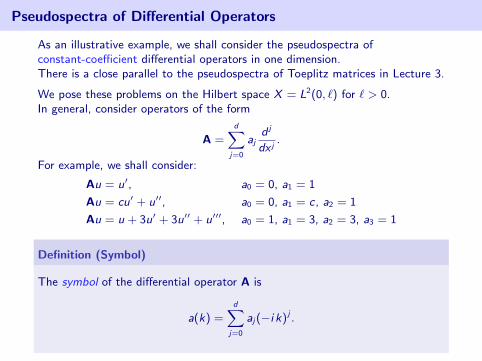
As an illustrative example, we shall consider the pseudospectra ofconstant-coefficient differential operators in one dimension.There is a close parallel to the pseudospectra of Toeplitz matrices in Lecture 3.
We pose these problems on the Hilbert space X = L2(0, `) for ` > 0.In general, consider operators of the form
A =dX
j=0
ajd j
dx j.
For example, we shall consider:
Au = u′, a0 = 0, a1 = 1
Au = cu′ + u′′, a0 = 0, a1 = c, a2 = 1
Au = u + 3u′ + 3u′′ + u′′′, a0 = 1, a1 = 3, a2 = 3, a3 = 1
Definition (Symbol)
The symbol of the differential operator A is
a(k) =dX
j=0
aj(−i k)j .
Pseudospectra of Differential Operators
As an illustrative example, we shall consider the pseudospectra ofconstant-coefficient differential operators in one dimension.There is a close parallel to the pseudospectra of Toeplitz matrices in Lecture 3.
We pose these problems on the Hilbert space X = L2(0, `) for ` > 0.In general, consider operators of the form
A =dX
j=0
ajd j
dx j.
For example, we shall consider:
Au = u′, a0 = 0, a1 = 1
Au = cu′ + u′′, a0 = 0, a1 = c, a2 = 1
Au = u + 3u′ + 3u′′ + u′′′, a0 = 1, a1 = 3, a2 = 3, a3 = 1
Definition (Symbol)
The symbol of the differential operator A is
a(k) =dX
j=0
aj(−i k)j .

Symbol Curve
A =dX
j=0
ajd j
dx j, a(k) =
dXj=0
aj(−i k)j .
The symbol curve is more complicated than for the a(T) for Toeplitz matrices.
For R > 0, define ΓR to be the real interval [−R,R] with endpoints joined bythe semicircle of radius R centered at zero in the upper half-plane.
Then consider the image of ΓR under a as R →∞.
ΓR for R = 2

Symbol Curve
A =dX
j=0
ajd j
dx j, a(k) =
dXj=0
aj(−i k)j .
The symbol curve is more complicated than for the a(T) for Toeplitz matrices.
For R > 0, define ΓR to be the real interval [−R,R] with endpoints joined bythe semicircle of radius R centered at zero in the upper half-plane.Then consider the image of ΓR under a as R →∞.
ΓR for R = 2 a(ΓR) for R = 2

Symbol Curve
A =dX
j=0
ajd j
dx j, a(k) =
dXj=0
aj(−i k)j .
The symbol curve is more complicated than for the a(T) for Toeplitz matrices.
For R > 0, define ΓR to be the real interval [−R,R] with endpoints joined bythe semicircle of radius R centered at zero in the upper half-plane.Then consider the image of ΓR under a as R →∞.
ΓR for R = 4 a(ΓR) for R = 4

Symbol Curve: Winding Number
A =dX
j=0
ajd j
dx j, a(k) =
dXj=0
aj(−i k)j .
For R > 0, define ΓR to be the real interval [−R,R] with endpoints joined bythe semicircle of radius R centered at zero in the upper half-plane.
Definition
For any λ 6∈ a(R), let I (a, λ) be the winding number of a(ΓR) about λ forsufficiently large R.
a(ΓR) for R = 4 a(ΓR) for R = 4 (zoom)
2 0
1
Pseudospectra of Differential Operators
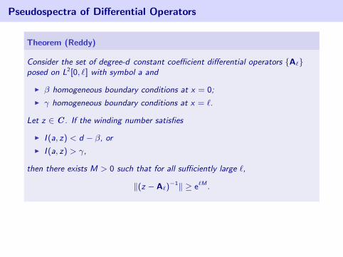
Theorem (Reddy)
Consider the set of degree-d constant coefficient differential operators {A`}posed on L2[0, `] with symbol a and
I β homogeneous boundary conditions at x = 0;
I γ homogeneous boundary conditions at x = `.
Let z ∈ C . If the winding number satisfies
I I (a, z) < d − β, or
I I (a, z) > γ,
then there exists M > 0 such that for all sufficiently large `,
‖(z − A`)−1‖ ≥ e`M .

Pseudospectra of Differential Operators: example 1
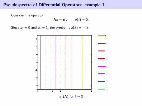
Consider the operatorAu = u′, u(`) = 0.
Since a0 = 0 and a1 = 1, the symbol is a(k) = −ik.
a(ΓR) for R = 2
10

Pseudospectra of Differential Operators: example 1
Consider the operatorAu = u′, u(`) = 0.
Since a0 = 0 and a1 = 1, the symbol is a(k) = −ik.
σε(A) for ` = 1

Pseudospectra of Differential Operators: example 1
Consider the operatorAu = u′, u(`) = 0.
Since a0 = 0 and a1 = 1, the symbol is a(k) = −ik.
σε(A) for ` = 2
Pseudospectra of Differential Operators: example 1
Consider the operatorAu = u′, u(`) = 0.
Since a0 = 0 and a1 = 1, the symbol is a(k) = −ik.
σε(A) for ` = 3

Pseudospectra of Differential Operators: example 2
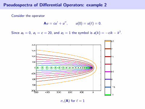
Consider the operator
Au = cu′ + u′′, u(0) = u(`) = 0.
Since a0 = 0, a1 = c = 20, and a2 = 1 the symbol is a(k) = −cik − k2.
a(ΓR) for R = 8
10
Pseudospectra of Differential Operators: example 2
Consider the operator
Au = cu′ + u′′, u(0) = u(`) = 0.
Since a0 = 0, a1 = c = 20, and a2 = 1 the symbol is a(k) = −cik − k2.
σε(A) for ` = 1
Pseudospectra of Differential Operators: example 2
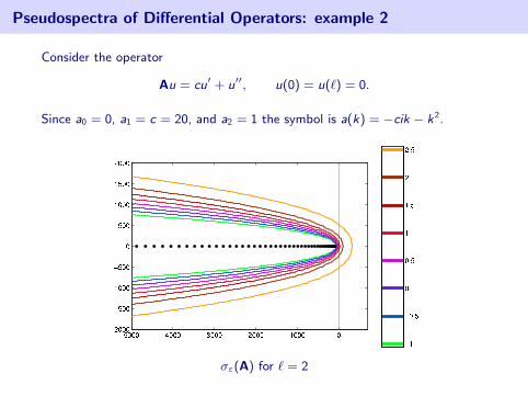
Consider the operator
Au = cu′ + u′′, u(0) = u(`) = 0.
Since a0 = 0, a1 = c = 20, and a2 = 1 the symbol is a(k) = −cik − k2.
σε(A) for ` = 2


