Download - Practical considerations in the optimization of flow production systems

This article was downloaded by: [University of Illinois Chicago]On: 08 December 2014, At: 14:34Publisher: Taylor & FrancisInforma Ltd Registered in England and Wales Registered Number: 1072954Registered office: Mortimer House, 37-41 Mortimer Street, London W1T 3JH, UK

International Journal of ProductionResearchPublication details, including instructions for authors andsubscription information:http://www.tandfonline.com/loi/tprs20

Practical considerations in theoptimization of flow productionsystemsHorst Tempelmeier aa Universität zu Köln, Seminar für produktionswirtschaft ,Albertus-Magnus-Platz, Kö ln, D-50923, Germany E-mail:Published online: 14 Nov 2010.

To cite this article: Horst Tempelmeier (2003) Practical considerations in the optimization offlow production systems, International Journal of Production Research, 41:1, 149-170, DOI:10.1080/00207540210161641

To link to this article: http://dx.doi.org/10.1080/00207540210161641

PLEASE SCROLL DOWN FOR ARTICLE

Taylor & Francis makes every effort to ensure the accuracy of all the information(the “Content”) contained in the publications on our platform. However, Taylor& Francis, our agents, and our licensors make no representations or warrantieswhatsoever as to the accuracy, completeness, or suitability for any purpose of theContent. Any opinions and views expressed in this publication are the opinions andviews of the authors, and are not the views of or endorsed by Taylor & Francis. Theaccuracy of the Content should not be relied upon and should be independentlyverified with primary sources of information. Taylor and Francis shall not be liablefor any losses, actions, claims, proceedings, demands, costs, expenses, damages,and other liabilities whatsoever or howsoever caused arising directly or indirectly inconnection with, in relation to or arising out of the use of the Content.

This article may be used for research, teaching, and private study purposes. Anysubstantial or systematic reproduction, redistribution, reselling, loan, sub-licensing,systematic supply, or distribution in any form to anyone is expressly forbidden.Terms & Conditions of access and use can be found at http://www.tandfonline.com/page/terms-and-conditions

http://www.tandfonline.com/loi/tprs20

http://www.tandfonline.com/action/showCitFormats?doi=10.1080/00207540210161641

http://dx.doi.org/10.1080/00207540210161641

http://www.tandfonline.com/page/terms-and-conditions

http://www.tandfonline.com/page/terms-and-conditions

int. j. prod. res., 2003, vol. 41, no. 1, 149–170

Practical considerations in the optimization of flow production systems

HORST TEMPELMEIERy

In this paper we consider the problems faced by an industrial planner who isresponsible for the design of real-life asynchronous production lines under sto-chastic conditions that may be due to breakdowns or random processing times.Based on real-life system data, it is shown that a number of available algorithmsfor the performance evaluation of a given system configuration as well as analgorithm for determining the optimum buffer configuration can be successfullyapplied in industrial practice.

1. Introduction

Over the last ten years, much effort has been devoted to the development ofapproaches for the performance analysis and optimization of stochastic flow pro-duction systems with finite buffers between the processing stations. The current bodyof knowledge is presented in the papers of Dallery and Gershwin (1992),Papadopoulos and Heavey (1996) and Gershwin (2000) as well as in several mono-graphs on stochastic models of manufacturing systems, such as Visvanadham andNarahari (1992), Buzacott and Shanthikumar (1993), Papadopoulos et al. (1993),Askin and Standridge (1993), Gershwin (1994), and Altiok (1997).

In spite of the significant benefits resulting from the application of analyticalplanning methods (an award-winning practical case study performed at Hewlett-Packard is described by Burman et al. 1998), many industrial planners seem to berather reluctant to apply the available methods. As far as we know, only a very smallnumber of companies use analytical flow line models. In many cases, planners haveonly limited knowledge about the existence of practically applicable evaluationmethods.

If quantitative performance evaluation is carried out at all, then in almost anycase simulation is the only tool used. Optimization problems, such as buffer optimi-zation, are mainly solved through simple trial-and-error approaches, which sufferfrom the severe drawbacks of being both very time-consuming and providing solu-tions that are usually far from optimal. According to an empiricial study conductedin 43 German companies in 1989, analytical planning tools were not applied at all(Schoniger and Spingler 1989). This empirical evidence has not changed much.

Several researchers provide rules of thumb and general insights acquired throughthe in-depth study of different configurations of several hypothetical flow productionsystems. See Conway et al. (1988), Blumenfeld (1990), Baker (1993), Hillier et al.(1993), Baker et al. (1994), Powell and Pyke (1996), Hillier and So (1996), Liu andLin (1996), So (1997), Powell and Pyke (1998), Hillier (2000), and Enginarlar et al.

SECOND PROOFS C.K.M. –i:/T&F UK/Tprs/Tprs41-1/Prs-2135.3d– Int. Journal of Production Research (PRS) Paper 102135 Keyword

International Journal of Production Research ISSN 0020–7543 print/ISSN 1366–588X online # 2003 Taylor & Francis Ltd

http://www.tandf.co.uk/journals

DOI: 10.1080/00207540210161641

Revision received May 2002{Universitat zu Koln, Seminar fur produktionswirtschaft, Albertus-Magnus-Platz,

D-50923 Koln, Germany. e-mail: [email protected]

Dow

nloa

ded

by [

Uni

vers

ity o

f Il

linoi

s C

hica

go]

at 1

4:34

08

Dec

embe

r 20

14

(2002). Industrial planners often believe that an optimal flow line design can bedeveloped based on the experience they have acquired with similar past projects.

Unfortunately, in the problem domain considered, the value of experience israther limited. The reason is that even a small change of data or system character-istics may generate a considerably different behaviour of the system under study. Forexample, changing the failure characteristics of a station through the introduction ofa machine based on a different technology or slightly changing the processing time ata station may shift the bottleneck of the system with the need to rearrange the bufferscompletely. As every production line is obviously unique, it jeopardizes the economicefficiency if a flow line planner relies completely upon experience gathered fromobservations of other production lines. Therefore, tools are required that can pro-vide system-specific performance measures in a fast and reliable manner.

This paper is organized as follows. In section 2 we discuss several characteristicsof real-life production systems that can be covered by analytical planning methods.It is shown, that a planner must be provided with basically three algorithms in orderto find good performance approximations in a wide variety of practical situations.The quality of the algorithms is proved with the help of simulation on the basis ofhypothetical as well as real-life data. In section 3, several types of optimizationproblems that emerge in industrial planning practice are discussed. Section 4 con-tains our conclusion and discusses several issues regarding the practical applicationof the analytical methods described.

2. Performance analysis of industrial flow production systems

Industrial factory planners who are responsible for building up sufficient produc-tion capacity in an economical way are confronted with a number of design factorsthat have an effect on the throughput of a planned production system subject tostochastic influences (breakdowns, random processing times). In addition to techni-cal considerations, such as the definition of the processes and the specification of therequired production and material handling resources, there are several organiza-tional issues that have to be decided upon. In the following, we deal with the ques-tion of how the negative consequences caused by stochastic phenomena such asbreakdowns or the variability of the processing times can be predicted and howthe resulting loss of throughput can be regained through the introduction ofbuffer spaces between the stations.

Many flow production systems comprise special-purpose machines that repeti-tively perform a certain number of tasks on a single product type. In this case, theprocessing times are deterministic. Randomness arises from breakdown and repairprocesses. In the following we assume operation-dependent failures. Based on anempirical study, Inman (1999) comes to the conclusion that the widespread assump-tion of exponential times to failure and exponential repair times is acceptable inmany cases.

There are several situations where stochastic processing times must be taken intoaccount. First, if the task is repetitively performed by a human operator, thenprocessing times will usually be random, as a certain amount of variability is inher-ent in human nature. Empirical studies show that task durations of human operatorswill have a coefficient of variation that is considerably less than one, which would bethe case for an exponential distribution. Secondly, if a number of flexible automaticmachines or robots assigned to a station are able to process a mixture of productvariants in any sequence, then—from the point of view of an external observer—the

150 H. Tempelmeier


Dow

nloa

ded

by [

Uni

vers

ity o

f Il

linoi

s C

hica

go]

at 1

4:34

08

Dec

embe

r 20

14

processing times of the variants can be considered as random. For a recent empiricalanalysis of processing times in automobile welding shops see Inman (1999).

Many researchers providing algorithms for the analysis of flow production sys-tems with stochastic processing times assume that processing times are exponential.In addition, several approaches are applicable only if the mean processing times,failure characteristics, and buffer sizes of all stations are identical. It is believed thatin the (deterministic) line balancing phase the system characteristics are set up suchthat there will be no station that is much worse than all the others (with respect to theisolated throughput). However, in industry this is not always the case. Due totechnical constraints, many real-life systems have stations with non-identical meanprocessing times—even if automatic machines are used to process a single producttype. Differences in the mean processing times may also emerge as a result of asimultaneous buffer and workload allocation, as discussed in section 3.

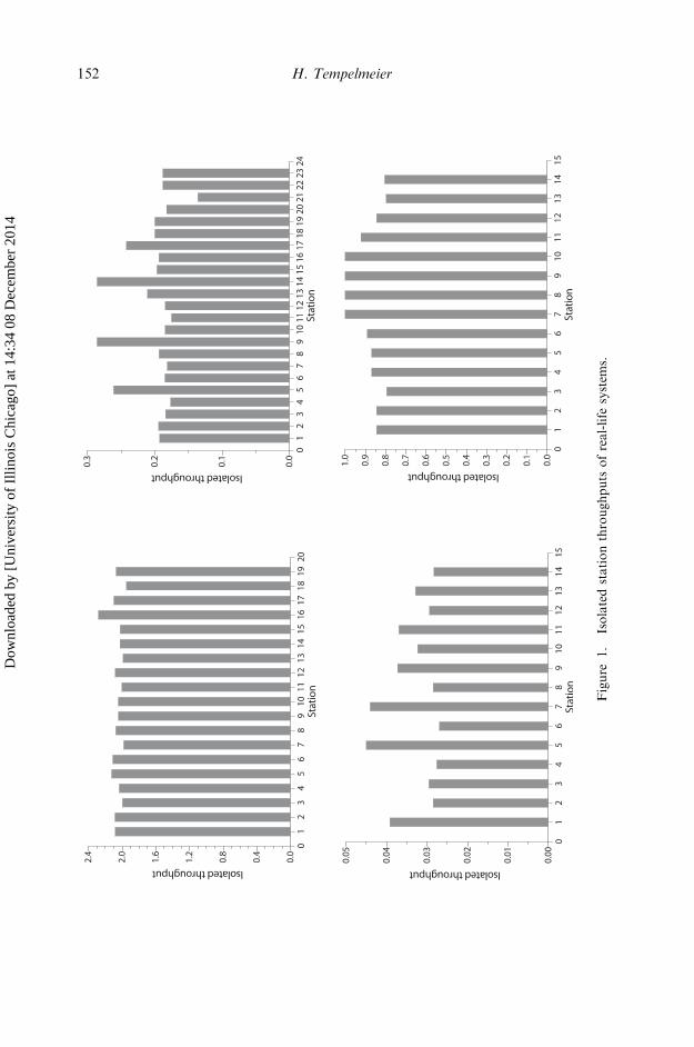
Figure 1 depicts the isolated station throughputs for four real-life linear flowproduction systems. The detailed data are given in the appendix. Observe that thedata exhibit a certain amount of imbalance, which makes many algorithms for theevaluation of stochastic flow production systems inapplicable or, at best, imprecise.

From the practical data presented, it is clear that an analytical flow line modelmust be able to cover unequal processing times. In addition, unequal failure andrepair characteristics must also be covered by such a model. In what follows, modelsand algorithms available for the approximate performance analysis of these types offlow production systems are tested with regard to their applicability in real-lifeplanning environments. From a practical point of view, the algorithms must beable to analyse systems with up to 50 or 100 stations, a requirement that excludesexact algorithms.

2.1. Deterministic processing timesIn a flow production system that comprises exclusively automatic stations work-

ing on a single part type, the processing times are usually deterministic but vary fromstation to station. This is often due to the fact that it is not possible to find combina-tions of subprocesses that sum to exactly the same processing time at all stations.Flow production systems of this kind can be analysed with the ‘Accelerated Dallery-David-Xie’ (ADDX) algorithm proposed by Burman (1995), which is based on thedecomposition method developed by Gershwin (1987) (see also Gershwin 1994) andwhich is an extension of the DDX-algorithm of Dallery et al. (1988). With respect tothe optimization algorithm discussed in section 3 it is noteworthy that the buffer sizesare modelled as continuous variables.

With the help of a large numerical experiment based on hypothetical system data,Burman (1995) showed that his algorithm was very accurate. In the following, thisalgorithm is applied to an invented system and several real-life systems.

Invented system 1Consider a system with invented data (ten stations with identical buffer sizes;

identical deterministic processing times s ¼ 1; identical failure processes at all sta-tions: failure rate f ¼ 0:007, repair rate r ¼ 0:095 (isolated throughput = 0.931)).Table 1 compares the system throughput found with the help of a SIMAN simula-tion model (Xsimulated) and with the ADDX algorithm (Xestimated).

151Optimization of flow production systems


Dow

nloa

ded

by [

Uni

vers

ity o

f Il

linoi

s C

hica

go]

at 1

4:34

08

Dec

embe

r 20

14

152 H. Tempelmeier


Figure

1.

Isolatedstationthroughputsofreal-life

system

s.

Dow

nloa

ded

by [

Uni

vers

ity o

f Il

linoi

s C

hica

go]

at 1

4:34

08

Dec

embe

r 20

14

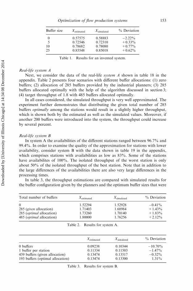
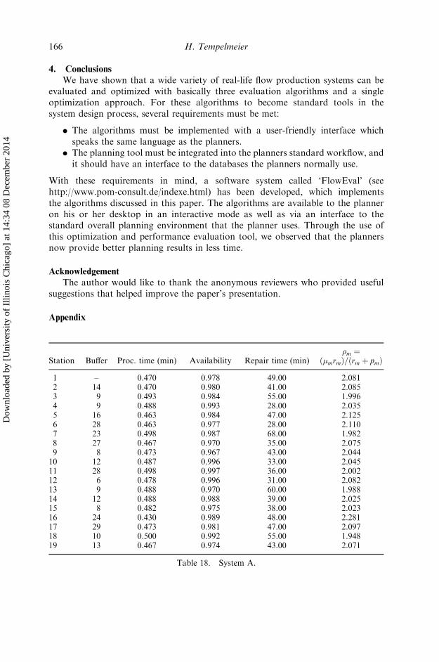
Real-life system ANext, we consider the data of the real-life system A shown in table 18 in the

appendix. Table 2 presents four scenarios with different buffer allocations: (1) zerobuffers; (2) allocation of 285 buffers provided by the industrial planners; (3) 285buffers allocated optimally with the help of the algorithm discussed in section 3;(4) target throughput of 1.8 with 485 buffers allocated optimally.

In all cases considered, the simulated throughput is very well approximated. Theexperiment further demonstrates that distributing the given total number of 285buffers optimally among the stations would result in a slightly higher throughput,which is shown both by the estimated as well as the simulated values. Moreover, ifanother 200 buffers were introduced into the system, the throughput could increaseby several percent.

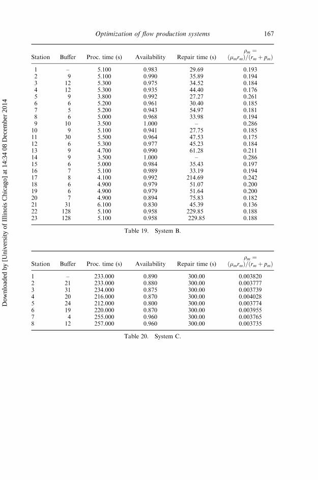
Real-life system BIn system A the availabilities of the different stations ranged between 96.7% and

99.4%. In order to examine the quality of the approximation for stations with loweravailability, consider system B with the data shown in table 19 in the appendix,which comprises stations with availabilities as low as 83%. Some of the stationshave availabilites of 100%. The isolated throughput of the worst station is onlyabout 50% of the isolated throughput of the best station. Note that in addition tothe large differences of the availabilities there are also very large differences in theprocessing times.

In table 3, the throughput estimations are compared with simulated results forthe buffer configuration given by the planners and the optimum buffer sizes that were



Buffer size Xestimated Xsimulated % Deviation

0 0.57575 0.58883 �2.22%5 0.72546 0.72310 +0.33%10 0.78682 0.78080 +0.77%25 0.85548 0.85018 +0.62%

Table 1. Results for an invented system.

Total number of buffers Xestimated Xsimulated % Deviation

0 1.52294 1.52928 �0.41%285 (given allocation) 1.71403 1.68984 +1.43%285 (optimal allocation) 1.73260 1.70140 +1.83%485 (optimal allocation) 1.80000 1.76256 +2.12%

Table 2. Results for system A.

Xestimated Xsimulated % Deviation

0 buffers 0.09238 0.10344 �10.70%1 buffer per station 0.11334 0.11503 �1.47%459 buffers (given allocation) 0.13474 0.13517 �0.32%193 buffers (optimal allocation) 0.13474 0.13300 1.31%

Table 3. Results for system B.

Dow

nloa

ded

by [

Uni

vers

ity o

f Il

linoi

s C

hica

go]

at 1

4:34

08

Dec

embe

r 20

14

required to provide the same estimated throughput. We also simulated a systemconfiguration without any buffers and one with a single buffer per station. For thecase of zero buffers, the algorithm is too pessimistic. However, if at least one buffer isincluded at every station, then the approximation is very good. In addition, it isobserved that the total number of buffers could be reduced from 459 to 193 if thesewere allocated optimally to the stations.

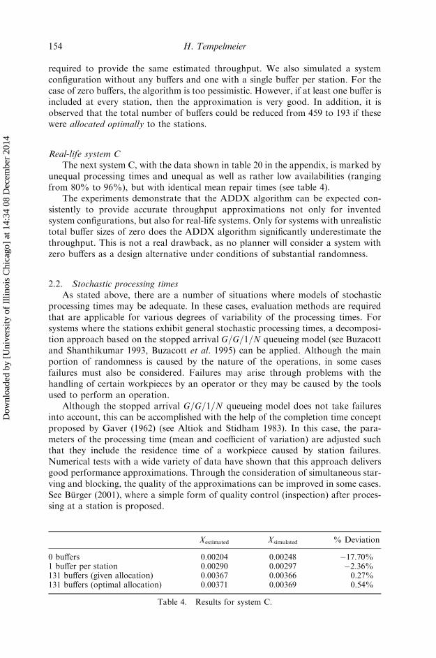
Real-life system CThe next system C, with the data shown in table 20 in the appendix, is marked by

unequal processing times and unequal as well as rather low availabilities (rangingfrom 80% to 96%), but with identical mean repair times (see table 4).

The experiments demonstrate that the ADDX algorithm can be expected con-sistently to provide accurate throughput approximations not only for inventedsystem configurations, but also for real-life systems. Only for systems with unrealistictotal buffer sizes of zero does the ADDX algorithm significantly underestimate thethroughput. This is not a real drawback, as no planner will consider a system withzero buffers as a design alternative under conditions of substantial randomness.

2.2. Stochastic processing timesAs stated above, there are a number of situations where models of stochastic

processing times may be adequate. In these cases, evaluation methods are requiredthat are applicable for various degrees of variability of the processing times. Forsystems where the stations exhibit general stochastic processing times, a decomposi-tion approach based on the stopped arrival G=G=1=N queueing model (see Buzacottand Shanthikumar 1993, Buzacott et al. 1995) can be applied. Although the mainportion of randomness is caused by the nature of the operations, in some casesfailures must also be considered. Failures may arise through problems with thehandling of certain workpieces by an operator or they may be caused by the toolsused to perform an operation.

Although the stopped arrival G=G=1=N queueing model does not take failuresinto account, this can be accomplished with the help of the completion time conceptproposed by Gaver (1962) (see Altiok and Stidham 1983). In this case, the para-meters of the processing time (mean and coefficient of variation) are adjusted suchthat they include the residence time of a workpiece caused by station failures.Numerical tests with a wide variety of data have shown that this approach deliversgood performance approximations. Through the consideration of simultaneous star-ving and blocking, the quality of the approximations can be improved in some cases.See Burger (2001), where a simple form of quality control (inspection) after proces-sing at a station is proposed.

154 H. Tempelmeier


Xestimated Xsimulated % Deviation

0 buffers 0.00204 0.00248 �17.70%1 buffer per station 0.00290 0.00297 �2.36%131 buffers (given allocation) 0.00367 0.00366 0.27%131 buffers (optimal allocation) 0.00371 0.00369 0.54%

Table 4. Results for system C.

Dow

nloa

ded

by [

Uni

vers

ity o

f Il

linoi

s C

hica

go]

at 1

4:34

08

Dec

embe

r 20

14

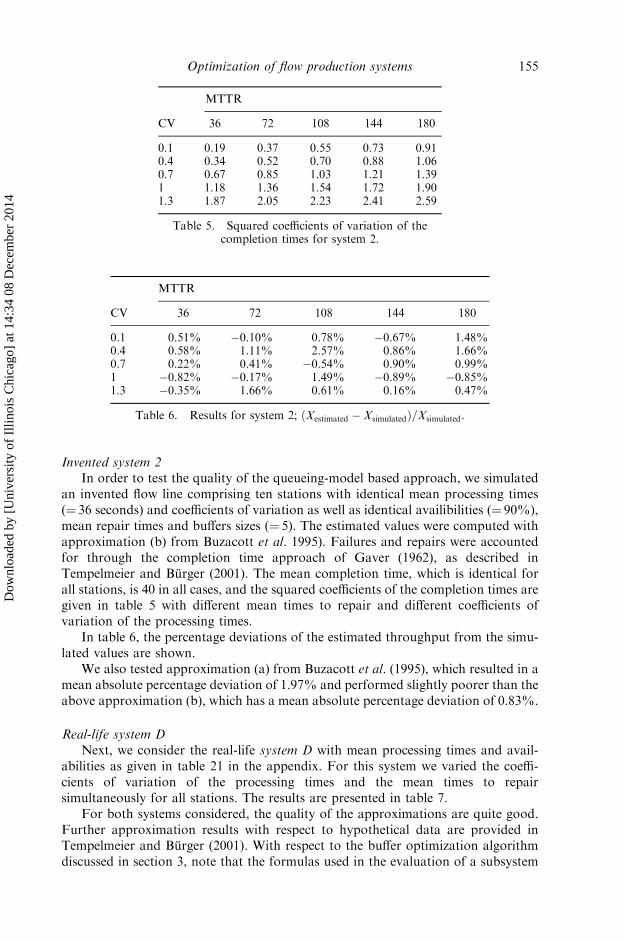
Invented system 2In order to test the quality of the queueing-model based approach, we simulated

an invented flow line comprising ten stations with identical mean processing times(¼ 36 seconds) and coefficients of variation as well as identical availibilities (¼ 90%),mean repair times and buffers sizes (¼ 5). The estimated values were computed withapproximation (b) from Buzacott et al. 1995). Failures and repairs were accountedfor through the completion time approach of Gaver (1962), as described inTempelmeier and Burger (2001). The mean completion time, which is identical forall stations, is 40 in all cases, and the squared coefficients of the completion times aregiven in table 5 with different mean times to repair and different coefficients ofvariation of the processing times.

In table 6, the percentage deviations of the estimated throughput from the simu-lated values are shown.

We also tested approximation (a) from Buzacott et al. (1995), which resulted in amean absolute percentage deviation of 1.97% and performed slightly poorer than theabove approximation (b), which has a mean absolute percentage deviation of 0.83%.

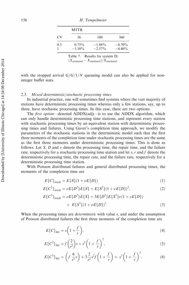
Real-life system DNext, we consider the real-life system D with mean processing times and avail-

abilities as given in table 21 in the appendix. For this system we varied the coeffi-cients of variation of the processing times and the mean times to repairsimultaneously for all stations. The results are presented in table 7.

For both systems considered, the quality of the approximations are quite good.Further approximation results with respect to hypothetical data are provided inTempelmeier and Burger (2001). With respect to the buffer optimization algorithmdiscussed in section 3, note that the formulas used in the evaluation of a subsystem



MTTR

CV 36 72 108 144 180

0.1 0.19 0.37 0.55 0.73 0.910.4 0.34 0.52 0.70 0.88 1.060.7 0.67 0.85 1.03 1.21 1.391 1.18 1.36 1.54 1.72 1.901.3 1.87 2.05 2.23 2.41 2.59

Table 5. Squared coefficients of variation of thecompletion times for system 2.

MTTR

CV 36 72 108 144 180

0.1 0.51% �0.10% 0.78% �0.67% 1.48%0.4 0.58% 1.11% 2.57% 0.86% 1.66%0.7 0.22% 0.41% �0.54% 0.90% 0.99%1 �0.82% �0.17% 1.49% �0.89% �0.85%1.3 �0.35% 1.66% 0.61% 0.16% 0.47%

Table 6. Results for system 2; ðXestimated � XsimulatedÞ=Xsimulated.

Dow

nloa

ded

by [

Uni

vers

ity o

f Il

linoi

s C

hica

go]

at 1

4:34

08

Dec

embe

r 20

14

with the stopped arrival G=G=1=N queueing model can also be applied for non-integer buffer sizes.

2.3. Mixed deterministic/stochastic processing timesIn industrial practice, one will sometimes find systems where the vast majority of

stations have deterministic processing times whereas only a few stations, say, up tothree, have stochastic processing times. In this case, there are two options.

The first option—denoted ADDX(adj)—is to use the ADDX algorithm, whichcan only handle deterministic processing time stations, and represent every stationwith stochastic processing times by an equivalent station with deterministic proces-sing times and failures. Using Gaver’s completion time approach, we modify theparameters of the stochastic stations in the deterministic model such that the firstthree moments of the completion time under stochastic processing times are the sameas the first three moments under deterministic processing times. This is done asfollows. Let S, D and � denote the processing time, the repair time, and the failurerate, respectively for a stochastic processing time station and let s, r and f denote thedeterministic processing time, the repair rate, and the failure rate, respectively for adeterministic processing time station.

With Poisson distributed failures and general distributed processing times, themoments of the completion time are

EfCgstoch ¼ EfSgð1þ �EfDgÞ ð1Þ

EfC2gstoch ¼ �EfD2gEfSg þ EfS2g 1þ �EfDgð Þ2; ð2Þ

EfC3gstoch ¼ �EfD3gEfSg þ 3EfD2gEfS2g� 1þ �EfDgð Þ

þ EfS3g 1þ �EfDgð Þ3 ð3Þ

When the processing times are deterministic with value s, and under the assumptionof Poisson distributed failures the first three moments of the completion time are

EfCgdet ¼ s

�1þ f

r

�; ð4Þ

EfC2gdet ¼ f2

r2

� �sþ s2 1þ f

r

� �2

; ð5Þ

EfC3gdet ¼ f6

r3s

� �þ 3

2

r2s2f 1þ f

r

� �þ s3 1þ f

r

� �3

: ð6Þ

156 H. Tempelmeier


MTTR

CV 36 180 360

0.5 0.75% �1.88% �4.70%1 �1.10% �2.57% �4.40%

Table 7. Results for system D;ðXestimated � XsimulatedÞ=Xsimulated.

Dow

nloa

ded

by [

Uni

vers

ity o

f Il

linoi

s C

hica

go]

at 1

4:34

08

Dec

embe

r 20

14

Setting EfCgstoch ¼ EfCgdet, EfC2gstoch ¼ EfC2gdet, and EfC3gstoch ¼ EfC3gdet, we

solve for the adjusted deterministic processing time s, the adjusted failure rate f , andthe adjusted repair rate r.

The solution of this system of equations is as follows:

s ¼ p

2n; ð7Þ

f ¼ 9q3

np; ð8Þ

r ¼ 3q

n; ð9Þ

with

n ¼ 2EfSg3g3 þ 3g�EfD2gðEfS2g � EfSg2Þ

þ EfS3gg3 � EfSgð3EfS2gg3 � �EfD3gÞ; ð10Þ

p ¼ 2EfSgEfS3gg4 � 3EfS2g2g4

þ EfSg4g4 þ EfSg2ð2EfD3g�g� 3�2EfD2g2Þ; ð11Þ

q ¼ EfSg�EfD2g þ ðEfS2g � EfSg2Þg2; ð12Þ

g ¼ 1þ �EfDg: ð13Þ

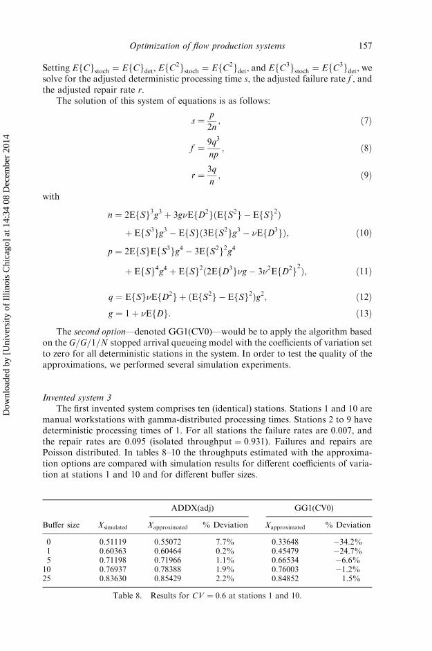
The second option—denoted GG1(CV0)—would be to apply the algorithm basedon the G=G=1=N stopped arrival queueing model with the coefficients of variation setto zero for all deterministic stations in the system. In order to test the quality of theapproximations, we performed several simulation experiments.

Invented system 3The first invented system comprises ten (identical) stations. Stations 1 and 10 are

manual workstations with gamma-distributed processing times. Stations 2 to 9 havedeterministic processing times of 1. For all stations the failure rates are 0.007, andthe repair rates are 0.095 (isolated throughput ¼ 0.931). Failures and repairs arePoisson distributed. In tables 8–10 the throughputs estimated with the approxima-tion options are compared with simulation results for different coefficients of varia-tion at stations 1 and 10 and for different buffer sizes.



ADDX(adj) GG1(CV0)

Buffer size Xsimulated Xapproximated % Deviation Xapproximated % Deviation

0 0.51119 0.55072 7.7% 0.33648 �34.2%1 0.60363 0.60464 0.2% 0.45479 �24.7%5 0.71198 0.71966 1.1% 0.66534 �6.6%10 0.76937 0.78388 1.9% 0.76003 �1.2%25 0.83630 0.85429 2.2% 0.84852 1.5%

Table 8. Results for CV ¼ 0:6 at stations 1 and 10.

Dow

nloa

ded

by [

Uni

vers

ity o

f Il

linoi

s C

hica

go]

at 1

4:34

08

Dec

embe

r 20

14

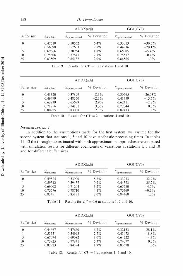
Invented system 4

In addition to the assumptions made for the first system, we assume for the

second system that stations 1, 5 and 10 have stochastic processing times. In tables

11–13 the throughputs estimated with both approximation approaches are compared

with simulation results for different coefficients of variations at stations 1, 5 and 10

and for different buffer sizes.

158 H. Tempelmeier


ADDX(adj) GG1(CV0)


0 0.47510 0.50562 6.4% 0.33013 �30.5%1 0.56098 0.57603 2.7% 0.44836 �20.1%5 0.69666 0.70954 1.8% 0.65905 �5.4%10 0.75806 0.77841 2.7% 0.75517 �0.4%25 0.83509 0.85182 2.0% 0.84565 1.3%

Table 9. Results for CV ¼ 1 at stations 1 and 10.

ADDX(adj) GG1(CV0)


0 0.41320 0.37899 �8.3% 0.30565 �26.03%1 0.49499 0.48350 �2.3% 0.41759 �15.6%5 0.63839 0.65699 2.9% 0.62411 �2.2%10 0.71756 0.74131 3.3% 0.72344 0.8%25 0.80925 0.83088 2.7% 0.82433 1.9%

Table 10. Results for CV ¼ 2 at stations 1 and 10.

ADDX(adj) GG1(CV0)


0 0.49525 0.53900 8.8% 0.33233 �32.9%1 0.59342 0.59437 0.2% 0.44373 �25.2%5 0.69002 0.71204 3.2% 0.65780 �4.7%10 0.75576 0.78710 4.1% 0.75369 �0.3%25 0.83451 0.85131 2.0% 0.84460 1.2%

Table 11. Results for CV ¼ 0:6 at stations 1, 5 and 10.

ADDX(adj) GG1(CV0)


0 0.44667 0.47660 6.7% 0.32133 �28.1%1 0.53551 0.54993 2.7% 0.43473 �18.8%5 0.67074 0.69082 3.0% 0.64222 �4.3%10 0.73925 0.77841 5.3% 0.74077 0.2%25 0.82823 0.84394 1.9% 0.83678 1.0%

Table 12. Results for CV ¼ 1 at stations 1, 5 and 10.

Dow

nloa

ded

by [

Uni

vers

ity o

f Il

linoi

s C

hica

go]

at 1

4:34

08

Dec

embe

r 20

14

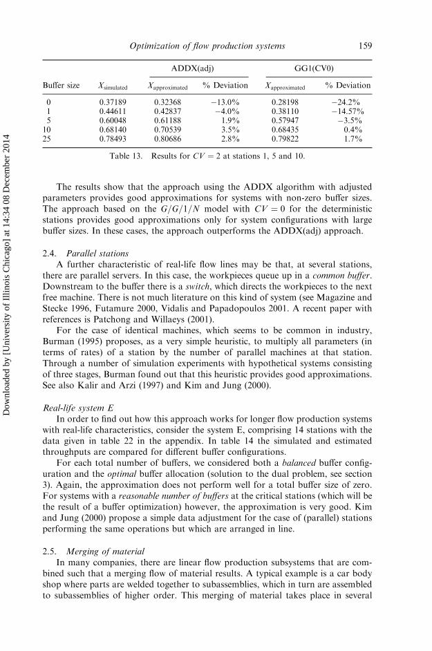
The results show that the approach using the ADDX algorithm with adjustedparameters provides good approximations for systems with non-zero buffer sizes.The approach based on the G=G=1=N model with CV ¼ 0 for the deterministicstations provides good approximations only for system configurations with largebuffer sizes. In these cases, the approach outperforms the ADDX(adj) approach.

2.4. Parallel stationsA further characteristic of real-life flow lines may be that, at several stations,

there are parallel servers. In this case, the workpieces queue up in a common buffer.Downstream to the buffer there is a switch, which directs the workpieces to the nextfree machine. There is not much literature on this kind of system (see Magazine andStecke 1996, Futamure 2000, Vidalis and Papadopoulos 2001. A recent paper withreferences is Patchong and Willaeys (2001).

For the case of identical machines, which seems to be common in industry,Burman (1995) proposes, as a very simple heuristic, to multiply all parameters (interms of rates) of a station by the number of parallel machines at that station.Through a number of simulation experiments with hypothetical systems consistingof three stages, Burman found out that this heuristic provides good approximations.See also Kalir and Arzi (1997) and Kim and Jung (2000).

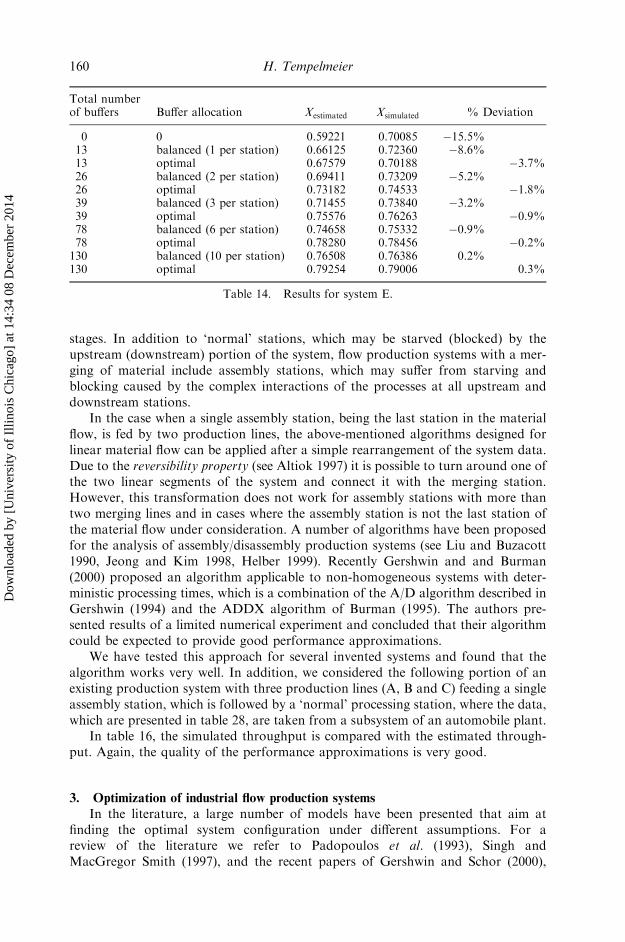
Real-life system EIn order to find out how this approach works for longer flow production systems

with real-life characteristics, consider the system E, comprising 14 stations with thedata given in table 22 in the appendix. In table 14 the simulated and estimatedthroughputs are compared for different buffer configurations.

For each total number of buffers, we considered both a balanced buffer config-uration and the optimal buffer allocation (solution to the dual problem, see section3). Again, the approximation does not perform well for a total buffer size of zero.For systems with a reasonable number of buffers at the critical stations (which will bethe result of a buffer optimization) however, the approximation is very good. Kimand Jung (2000) propose a simple data adjustment for the case of (parallel) stationsperforming the same operations but which are arranged in line.

2.5. Merging of materialIn many companies, there are linear flow production subsystems that are com-

bined such that a merging flow of material results. A typical example is a car bodyshop where parts are welded together to subassemblies, which in turn are assembledto subassemblies of higher order. This merging of material takes place in several



ADDX(adj) GG1(CV0)


0 0.37189 0.32368 �13.0% 0.28198 �24.2%1 0.44611 0.42837 �4.0% 0.38110 �14.57%5 0.60048 0.61188 1.9% 0.57947 �3.5%10 0.68140 0.70539 3.5% 0.68435 0.4%25 0.78493 0.80686 2.8% 0.79822 1.7%

Table 13. Results for CV ¼ 2 at stations 1, 5 and 10.

Dow

nloa

ded

by [

Uni

vers

ity o

f Il

linoi

s C

hica

go]

at 1

4:34

08

Dec

embe

r 20

14

stages. In addition to ‘normal’ stations, which may be starved (blocked) by theupstream (downstream) portion of the system, flow production systems with a mer-ging of material include assembly stations, which may suffer from starving andblocking caused by the complex interactions of the processes at all upstream anddownstream stations.

In the case when a single assembly station, being the last station in the materialflow, is fed by two production lines, the above-mentioned algorithms designed forlinear material flow can be applied after a simple rearrangement of the system data.Due to the reversibility property (see Altiok 1997) it is possible to turn around one ofthe two linear segments of the system and connect it with the merging station.However, this transformation does not work for assembly stations with more thantwo merging lines and in cases where the assembly station is not the last station ofthe material flow under consideration. A number of algorithms have been proposedfor the analysis of assembly/disassembly production systems (see Liu and Buzacott1990, Jeong and Kim 1998, Helber 1999). Recently Gershwin and and Burman(2000) proposed an algorithm applicable to non-homogeneous systems with deter-ministic processing times, which is a combination of the A/D algorithm described inGershwin (1994) and the ADDX algorithm of Burman (1995). The authors pre-sented results of a limited numerical experiment and concluded that their algorithmcould be expected to provide good performance approximations.

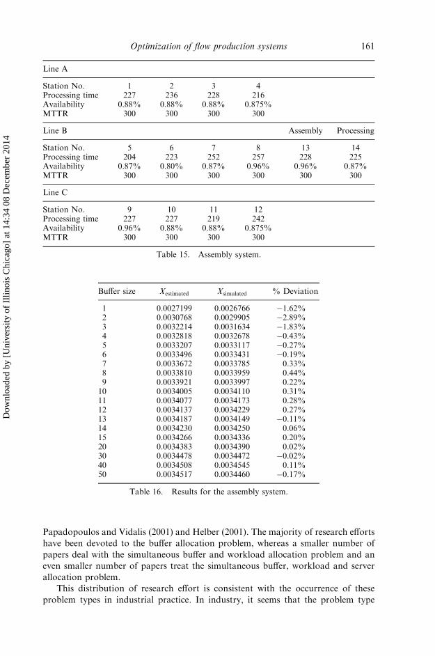
We have tested this approach for several invented systems and found that thealgorithm works very well. In addition, we considered the following portion of anexisting production system with three production lines (A, B and C) feeding a singleassembly station, which is followed by a ‘normal’ processing station, where the data,which are presented in table 28, are taken from a subsystem of an automobile plant.

In table 16, the simulated throughput is compared with the estimated through-put. Again, the quality of the performance approximations is very good.

3. Optimization of industrial flow production systems

In the literature, a large number of models have been presented that aim atfinding the optimal system configuration under different assumptions. For areview of the literature we refer to Padopoulos et al. (1993), Singh andMacGregor Smith (1997), and the recent papers of Gershwin and Schor (2000),

160 H. Tempelmeier


Total numberof buffers Buffer allocation Xestimated Xsimulated % Deviation

0 0 0.59221 0.70085 �15.5%13 balanced (1 per station) 0.66125 0.72360 �8.6%13 optimal 0.67579 0.70188 �3.7%26 balanced (2 per station) 0.69411 0.73209 �5.2%26 optimal 0.73182 0.74533 �1.8%39 balanced (3 per station) 0.71455 0.73840 �3.2%39 optimal 0.75576 0.76263 �0.9%78 balanced (6 per station) 0.74658 0.75332 �0.9%78 optimal 0.78280 0.78456 �0.2%130 balanced (10 per station) 0.76508 0.76386 0.2%130 optimal 0.79254 0.79006 0.3%

Table 14. Results for system E.

Dow

nloa

ded

by [

Uni

vers

ity o

f Il

linoi

s C

hica

go]

at 1

4:34

08

Dec

embe

r 20

14

Papadopoulos and Vidalis (2001) and Helber (2001). The majority of research efforts

have been devoted to the buffer allocation problem, whereas a smaller number of

papers deal with the simultaneous buffer and workload allocation problem and an

even smaller number of papers treat the simultaneous buffer, workload and server

allocation problem.

This distribution of research effort is consistent with the occurrence of these

problem types in industrial practice. In industry, it seems that the problem type



Line A

Station No. 1 2 3 4Processing time 227 236 228 216Availability 0.88% 0.88% 0.88% 0.875%MTTR 300 300 300 300

Line B Assembly Processing

Station No. 5 6 7 8 13 14Processing time 204 223 252 257 228 225Availability 0.87% 0.80% 0.87% 0.96% 0.96% 0.87%MTTR 300 300 300 300 300 300

Line C

Station No. 9 10 11 12Processing time 227 227 219 242Availability 0.96% 0.88% 0.88% 0.875%MTTR 300 300 300 300

Table 15. Assembly system.

Buffer size Xestimated Xsimulated % Deviation

1 0.0027199 0.0026766 �1.62%2 0.0030768 0.0029905 �2.89%3 0.0032214 0.0031634 �1.83%4 0.0032818 0.0032678 �0.43%5 0.0033207 0.0033117 �0.27%6 0.0033496 0.0033431 �0.19%7 0.0033672 0.0033785 0.33%8 0.0033810 0.0033959 0.44%9 0.0033921 0.0033997 0.22%10 0.0034005 0.0034110 0.31%11 0.0034077 0.0034173 0.28%12 0.0034137 0.0034229 0.27%13 0.0034187 0.0034149 �0.11%14 0.0034230 0.0034250 0.06%15 0.0034266 0.0034336 0.20%20 0.0034383 0.0034390 0.02%30 0.0034478 0.0034472 �0.02%40 0.0034508 0.0034545 0.11%50 0.0034517 0.0034460 �0.17%

Table 16. Results for the assembly system.

Dow

nloa

ded

by [

Uni

vers

ity o

f Il

linoi

s C

hica

go]

at 1

4:34

08

Dec

embe

r 20

14

considered most frequently is the buffer allocation problem (finding the minimumnumber of buffers required to achieve a given throughput). Depending on the posi-tion of the planners in the factory planning workflow, sometimes a wider perspectiveis taken that also includes the determination of the cycle times for the stations, withan implicit consideration of the consequences for the allocation of the machines orrobots among the stations.

3.1. Buffer optimizationAs a single buffer unit may represent a considerable amount of investment, up to

several thousand US dollars, and also requires scarce factory space, and as theplanners normally must treat the throughput of the production system to be plannedas a datum, they usually aim at minimizing the total number of buffers, N, withrespect to a desired throughput level Xmin. In the literature this problem is called the‘primal problem’ (Minimize N ¼

Pbm with respect to XðbÞ Xmin, where bm

denotes the buffer size of station m). It is interrelated with the so-called ‘dual pro-blem’ (Maximize XðbÞ w.r.t.

Pbm ¼ N), which means to allocate a given total

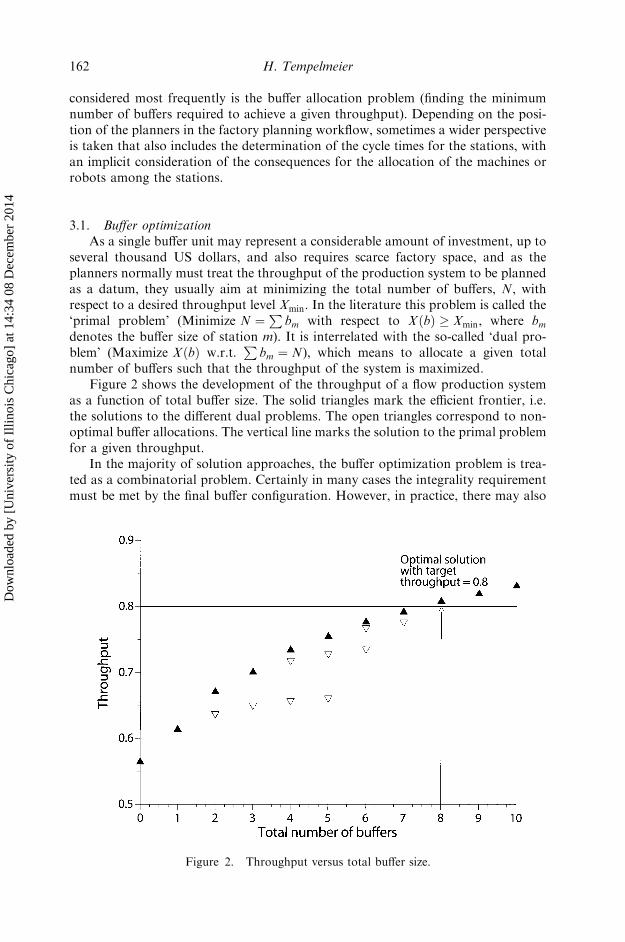
number of buffers such that the throughput of the system is maximized.Figure 2 shows the development of the throughput of a flow production system

as a function of total buffer size. The solid triangles mark the efficient frontier, i.e.the solutions to the different dual problems. The open triangles correspond to non-optimal buffer allocations. The vertical line marks the solution to the primal problemfor a given throughput.

In the majority of solution approaches, the buffer optimization problem is trea-ted as a combinatorial problem. Certainly in many cases the integrality requirementmust be met by the final buffer configuration. However, in practice, there may also

162 H. Tempelmeier


Figure 2. Throughput versus total buffer size.

Dow

nloa

ded

by [

Uni

vers

ity o

f Il

linoi

s C

hica

go]

at 1

4:34

08

Dec

embe

r 20

14

be cases where buffer sizes are expressed in such a dimension that non-integer buffersizes make some sense. A case where this is true is a filling line for ketchup bottles,where the buffer size is measured in units of 100 bottles. Physically there were buffersof size, say 2550 bottles, which would be 25.5 units. In addition, if the algorithm usedfor the performance evaluation of a given system configuration is also capable ofanalysing systems with non-integer buffer sizes, then a very efficient approach pro-posed by Schor (1995) (see also Gershwin and Schor 2000) can be used to solve thebuffer optimization problem. As pointed out earlier, non-integer buffer sizes can behandled with all the performance evaluation algorithms that we have used in section2. Therefore, Schor’s optimization algorithm can be combined with all evaluationapproaches to solve the buffer optimization problem efficiently and accurately underconditions of deterministic as well as stochastic processing times, even for determi-nistic processing time systems with merging material flow.

As there is no closed-form equation available that describes the development ofthe throughput versus total buffer size, Schor (1995) divides the problem into twoparts, (a) the dual problem of finding the maximum throughput for a given totalbuffer size and (b) the primal problem of finding the minimum total number ofbuffers required to achieve a target throughput level. The dual problem is solvedthrough a gradient-based search, while the primal problem is solved through succes-sive linear approximations of the throughput curve, which is evaluated through thesolution of several instances of the dual problem. After the algorithm has stopped,the buffers are rounded with a procedure that leaves the total buffer size unchanged.

Whenever we referred to optimal allocations for the systems considered in section2, we used a variant of Schor’s algorithm to find them. This algorithm can also easilybe modified to consider the following additional practical requirements:

. Fixed buffer size at a station (defined by the planner due to technical con-straints).

. Minimum buffer size at a station.

. Maximum buffer size at a station.

3.2. Buffer and cycle time optimizationIf the planner has a wider perspective, then not only the buffer sizes, but also the

number of servers at a station and the workload assigned to a station may bedecision variables. A rather general model formulation originally proposed byHillier and So (1995) is considered by Spinellis et al. (2000). They consider as vari-ables the buffer sizes, the workloads and the numbers of workers with the objectivefunction of maximizing the throughput of the flow production system. Each type ofvariable is restricted such that the total number of buffers, the total workload andthe total number of servers is constant. This problem formulation is solved with thehelp of a simulated annealing procedure.

A similar model formulation, which is based on a practical case study at theGerman car manufacturer BMW, is described by Spieckermann et al. (2000). Theyconsider a planning problem that arises in the early stages of the car body shopplanning process. From the preceding planning phase a target throughput Xmin isgiven. The objective is to find the minimum of a function with positive coefficientsfor the buffer space used and with negative coefficients for cycle times at the stations.The planning problem reads as follows:



Dow

nloa

ded

by [

Uni

vers

ity o

f Il

linoi

s C

hica

go]

at 1

4:34

08

Dec

embe

r 20

14

Minimize Z ¼ f ðb;wÞ; ð14Þ

s:t:

Xðb;wÞ Xmin; ð15Þ

Wminm wm Wmax

m m ¼ 1; 2; . . . ;M; ð16Þ

bm ¼ integer m ¼ 1; 2; . . . ;M; ð17Þ

wm 0 m ¼ 1; 2; . . . ;M: ð18Þ

Decision variables are bm (buffer size at station m) and wm (cycle time at station m).The term Xð�Þ denotes the throughput of the system, which depends on the bufferconfiguration and the workload allocation. The motivation for this problem formu-lation is based on the aggregate view of the car body shop, where each cell isconsidered as a black box. The structure of these black boxes is only fixed in sub-sequent planning stages. The maximum cycle time is computed on the basis of atarget throughput per day and the minimum cycle time results from technical con-siderations with respect to the resources included in a cell.

Owing to the random nature of the failure and repair processes the targetthroughput will only be achieved if a large number of buffers is put between thestations, with the effect that no production is lost due to starvation or blockages. In azero-buffer system configuration, a large amout of throughput would be lost due tostarvation and blockages. This loss of throughput can be regained through anincrease of the buffer sizes and/or a reduction of the cycle times.

In the practical planning environment, the cycle time of a station is considered asa decision variable that has an influence on the number of resources (robots)required at station m. For example, with a cycle time of 250 seconds, say, fivewelding robots may be necessary, whereas for a processing time of 220 one addi-tional robot is needed. Obviously, in this case, a new allocation of the workload tothe changed number of resources must be found. With robots this will be no pro-blem. As a robot is costly, an important part of the objective function is to set theprocessing times as large as possible.

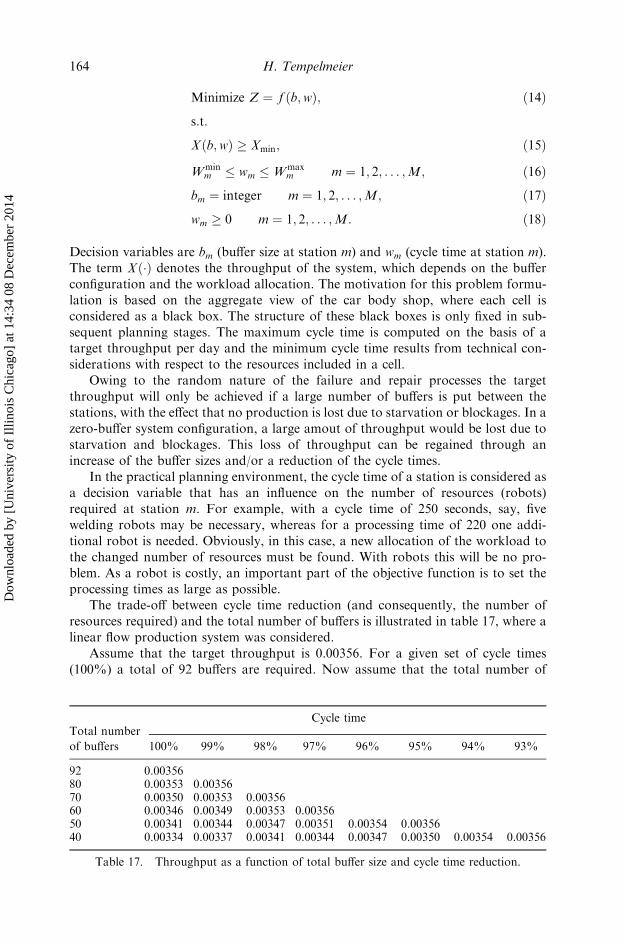
The trade-off between cycle time reduction (and consequently, the number ofresources required) and the total number of buffers is illustrated in table 17, where alinear flow production system was considered.

Assume that the target throughput is 0.00356. For a given set of cycle times(100%) a total of 92 buffers are required. Now assume that the total number of

164 H. Tempelmeier


Cycle timeTotal number

of buffers 100% 99% 98% 97% 96% 95% 94% 93%

92 0.0035680 0.00353 0.0035670 0.00350 0.00353 0.0035660 0.00346 0.00349 0.00353 0.0035650 0.00341 0.00344 0.00347 0.00351 0.00354 0.0035640 0.00334 0.00337 0.00341 0.00344 0.00347 0.00350 0.00354 0.00356

Table 17. Throughput as a function of total buffer size and cycle time reduction.

Dow

nloa

ded

by [

Uni

vers

ity o

f Il

linoi

s C

hica

go]

at 1

4:34

08

Dec

embe

r 20

14

buffers is reduced to 80, 70, 60, . . . , 40. With unmodified cycle times, the throughputwould reduce to 0.00334, as shown in the ‘100%’-column of table 17. The remainingentries in the table show the throughput that would be achieved if the cycle times atall stations were simultaneously reduced to the percentage denoted in the columnheader and if the total number of buffers (given in the row header) were reallocatedoptimally among the stations (solution of the dual problem). Observe that the cycletime reduction required to regain the production loss caused by the reduction ofbuffer sizes depends on the number of buffers.

In the practical planning environment, Spieckermann et al. (2000) use a geneticalgorithm that is combined with a simulation model of the body shop. The fitnessfunction comprises the buffer sizes, deviations of the processing times from theirupper bounds as well as the unbalancedness of the processing times. The geneticalgorithm calls a simulation model for the performance evaluation of the aggregatecar body shop. As far as we know, this approach has become standard in theplanning practice of BMW and is also used by other European car manufacturers.However, the computation times required by the GA/simulation approach are extre-mely long, usually several days, and the solution found in this way can probably befurther improved.

As an alternative, the speed of the optimization could be increased along twodifferent lines. Instead of the genetic algorithm, a specialized optimization algorithm,at least for a subset of the problem variables could be used. Instead of simulation, ananalytical algorithm for the evaluation of the system could be applied.

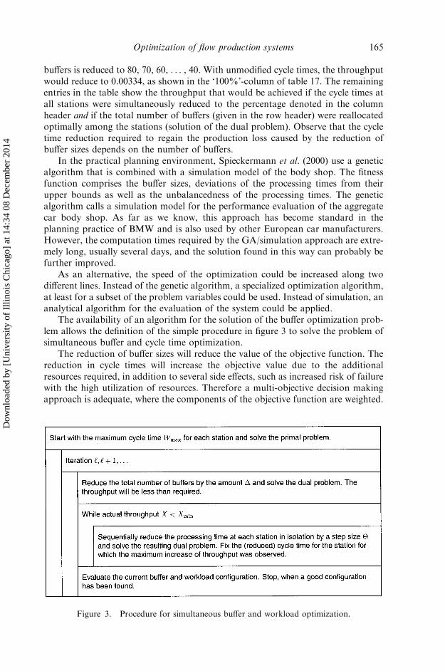
The availability of an algorithm for the solution of the buffer optimization prob-lem allows the definition of the simple procedure in figure 3 to solve the problem ofsimultaneous buffer and cycle time optimization.

The reduction of buffer sizes will reduce the value of the objective function. Thereduction in cycle times will increase the objective value due to the additionalresources required, in addition to several side effects, such as increased risk of failurewith the high utilization of resources. Therefore a multi-objective decision makingapproach is adequate, where the components of the objective function are weighted.



Figure 3. Procedure for simultaneous buffer and workload optimization.

Dow

nloa

ded

by [

Uni

vers

ity o

f Il

linoi

s C

hica

go]

at 1

4:34

08

Dec

embe

r 20

14

4. Conclusions

We have shown that a wide variety of real-life flow production systems can beevaluated and optimized with basically three evaluation algorithms and a singleoptimization approach. For these algorithms to become standard tools in thesystem design process, several requirements must be met:

. The algorithms must be implemented with a user-friendly interface whichspeaks the same language as the planners.

. The planning tool must be integrated into the planners standard workflow, andit should have an interface to the databases the planners normally use.

With these requirements in mind, a software system called ‘FlowEval’ (seehttp://www.pom-consult.de/indexe.html) has been developed, which implementsthe algorithms discussed in this paper. The algorithms are available to the planneron his or her desktop in an interactive mode as well as via an interface to thestandard overall planning environment that the planner uses. Through the use ofthis optimization and performance evaluation tool, we observed that the plannersnow provide better planning results in less time.

Acknowledgement

The author would like to thank the anonymous reviewers who provided usefulsuggestions that helped improve the paper’s presentation.

Appendix

166 H. Tempelmeier


�m ¼Station Buffer Proc. time (min) Availability Repair time (min) ð�mrmÞ=ðrm þ pmÞ

1 – 0.470 0.978 49.00 2.0812 14 0.470 0.980 41.00 2.0853 9 0.493 0.984 55.00 1.9964 9 0.488 0.993 28.00 2.0355 16 0.463 0.984 47.00 2.1256 28 0.463 0.977 28.00 2.1107 23 0.498 0.987 68.00 1.9828 27 0.467 0.970 35.00 2.0759 8 0.473 0.967 43.00 2.04410 12 0.487 0.996 33.00 2.04511 28 0.498 0.997 36.00 2.00212 6 0.478 0.996 31.00 2.08213 9 0.488 0.970 60.00 1.98814 12 0.488 0.988 39.00 2.02515 8 0.482 0.975 38.00 2.02316 24 0.430 0.989 48.00 2.28117 29 0.473 0.981 47.00 2.09718 10 0.500 0.992 55.00 1.94819 13 0.467 0.974 43.00 2.071

Table 18. System A.

Dow

nloa

ded

by [

Uni

vers

ity o

f Il

linoi

s C

hica

go]

at 1

4:34

08

Dec

embe

r 20

14



�m ¼Station Buffer Proc. time (s) Availability Repair time (s) ð�mrmÞ=ðrm þ pmÞ

1 – 5.100 0.983 29.69 0.1932 9 5.100 0.990 35.89 0.1943 12 5.300 0.975 34.52 0.1844 12 5.300 0.935 44.40 0.1765 9 3.800 0.992 27.27 0.2616 6 5.200 0.961 30.40 0.1857 5 5.200 0.943 54.97 0.1818 6 5.000 0.968 33.98 0.1949 10 3.500 1.000 – 0.28610 9 5.100 0.941 27.75 0.18511 30 5.500 0.964 47.53 0.17512 6 5.300 0.977 45.23 0.18413 9 4.700 0.990 61.28 0.21114 9 3.500 1.000 – 0.28615 6 5.000 0.984 35.43 0.19716 7 5.100 0.989 33.19 0.19417 8 4.100 0.992 214.69 0.24218 6 4.900 0.979 51.07 0.20019 6 4.900 0.979 51.64 0.20020 7 4.900 0.894 75.83 0.18221 31 6.100 0.830 45.39 0.13622 128 5.100 0.958 229.85 0.18823 128 5.100 0.958 229.85 0.188

Table 19. System B.

�m ¼Station Buffer Proc. time (s) Availability Repair time (s) ð�mrmÞ=ðrm þ pmÞ

1 – 233.000 0.890 300.00 0.0038202 21 233.000 0.880 300.00 0.0037773 31 234.000 0.875 300.00 0.0037394 20 216.000 0.870 300.00 0.0040285 24 212.000 0.800 300.00 0.0037746 19 220.000 0.870 300.00 0.0039557 4 255.000 0.960 300.00 0.0037658 12 257.000 0.960 300.00 0.003735

Table 20. System C.

Dow

nloa

ded

by [

Uni

vers

ity o

f Il

linoi

s C

hica

go]

at 1

4:34

08

Dec

embe

r 20

14

References

Altiok, T., 1997, Performance Analysis of Manufacturing Systems (New York: Springer).Altiok, T. and Stidham, S., 1983, The allocation of interstage buffer capacities in production

lines. IIE Transactions, 15, 292–299.Askin, R. and Standridge, C., 1993, Modeling and Analysis of Manufacturing Systems (New

York: Wiley).Baker, K. R., 1993, Tightly-coupled production systems: models, analysis, and insights.

Journal of Manufacturing Systems, 11(6), 385–400.Baker, K. R., Powell, S. G. and Pyke, D. F., 1994, A predictive model for the throughput

of unbalanced, unbufferred three-station serial lines. IIE Transactions, 26, 62–71.Blumenfeld, D. E., 1990, A simple formula for estimating throughput of serial production

lines with variable processing times and limited buffer capacity. International Journal ofProduction Research, 28, 1163–1182.

Burman, M. H., 1995, New results in flow line analysis. PhD thesis, Massachussetts Instituteof Technology, Cambridge, MA.

168 H. Tempelmeier


Station Buffer Proc. time (s) Availability �m ¼ ð�mrmÞ=ðrm þ pmÞ

1 – 25.000 0.980 0.0392 8 34.00 0.970 0.0293 25 33.500 0.990 0.0304 1 35.500 0.980 0.0285 2 22.000 0.990 0.0456 16 36.00 0.970 0.0277 7 22.000 0.970 0.0448 32 34.000 0.970 0.0299 1 26.000 0.970 0.03710 8 30.000 0.970 0.03211 20 26.500 0.980 0.03712 9 33.000 0.970 0.02913 21 29.500 0.970 0.03314 16 35.000 0.990 0.028

Table 21. System D.

�m ¼Station Servers Proc. time (min) Availability Repair time (min) ð�mrmÞ=ðrm þ pmÞ

1 1 1.1 0.930 9.70 0.8452 2 1.1 0.930 9.70 0.8453 1 1.17 0.930 12.00 0.7954 1 1.07 0.930 12.00 0.8695 2 1.07 0.930 12.00 0.8696 2 1.1 0.980 3.20 0.8917 2 0.85 0.850 19.00 1.0008 2 0.85 0.850 19.00 1.0009 2 0.85 0.850 19.00 1.00010 2 0.85 0.850 19.00 1.00011 3 1.063 0.980 3.20 0.92212 2 1.1 0.930 12.00 0.84513 2 1.23 0.980 4.50 0.79714 2 1.18 0.950 12.00 0.805

Table 22. System E.

Dow

nloa

ded

by [

Uni

vers

ity o

f Il

linoi

s C

hica

go]

at 1

4:34

08

Dec

embe

r 20

14

Burman, M., Gershwin, S. B. and Suyematsu, C., 1998, Hewlett-Packard uses operationsresearch to improve the design of a printer production line. Interfaces, 28(1), 24–36.

Buzacott, J. A. and Shanthikumar, J. G., 1993, Stochastic Models of ManufacturingSystems (Englewood Cliffs: Prentice Hall).

Buzacott, J., Liu, X.-G. and Shanthikumar, G., 1995, Multistage flow line analysis withthe stopped arrival queue model. IIE Transactions, 27, 444–455.

Conway, R., Maxwell, W., McClain, J. and Thomas, L., 1988. The role of work-in-process inventory in serial production lines. Operations Research, 36, 229–241.

Dallery, Y. and Gershwin, S. B., 1992, Manufacturing flow line systems: a review ofmodels and analytical results. Queueing Systems Theory and Applications, 12, 3–94.

Enginarlar, E., Li, J., Meerkov, S. and Zhang, R., 2002, Buffer capacity for accommodat-ing machine downtime in serial production lines. International Journal of ProductionResearch, 40, 601–624.

Futamura, K., 2000, The multiple server effect:optimal allocation of severs to stations withdifferent service-time distributions isn tandem queueing networks. Annals of OperationsResearch, 93, 71–90.

Gaver, D. P., 1962, A waiting line with interrupted service, including priorities. Journal of theRoyal Statistical Society, 24(1), 73–90.

Gershwin, S. B., 1987, An efficient decomposition algorithm for the approximate evaluationof tandem queues with finite storage space and blocking. Operations Research, 35,291–305.

Gershwin, S., 2000, Design and operation of manufacturing systems: the control-point pol-icy. IIE Transactions, 32, 891–906.

Gershwin, S. B., 1994, Manufacturing Systems Engineering (Englewood Cliffs, NJ: PrenticeHall).

Gershwin, S. B. and Burman, M. H., 2000. A decomposition method for analyzing inho-mogeneous Assembly/Dissassembly systems. Annals of Operations Research, 93, 91–115.

Gershwin, S. B. and Schor, J. E., 2000, Efficient algorithms for buffer space allocation.Annals of Operations Research, 93, 117–144.

Helber, S., 1999, Performance Analysis of Flow Lines with Non-Linear Flow of Material.Lecture Notes in Economics and Mathematical Systems (Berlin: Springer).

Helber, S., 2001, Cash-flow-oriented buffer allocation in stochastic flow lines. InternationalJournal of Production Research, 39, 3061–3083.

Hillier, M. S., 2000, Characterizing the optimal allocaiton of storaage space in productionline systems with variable rocessing times. IIE Transactions, 32, 1–8.

Hillier, F. and So, K., 1995, On the optimal design of tandem queueing systems with finitebuffers. Queueing Systems, 21, 245–266.

Hillier, F. S. and So, K. C., 1996, On the simultaneous optimization of server and workallocations in production line systems with variable processing times. OperationsResearch, 44, 435–443.

Hillier, F. S., So, K. C. and Boling, R.W., 1993, Notes: toward characterizing the optimumallocation of storage space in production line systems with variable processing times.Management Science, 39, 126–133.

Inman, R. R., 1999, Empirical evaluation of exponential and independence assumptions inqueueing model of manufacturing systems. Production and Operations Management,8(4), 409–432.

Jeong, K.-C. and Kim, Y.-D., 1998, Performance analysis of assembly/disassembly systemswith unreliable machines and random processing times. IIE Transactions, 30, 41–53.

Kalir, A. and Arzi, Y., 1997, Automated production line design with flexible unreliablemachines for profit maximization. International Journal of Production Research, 35,1651–1664.

Kim, D. and Jung, B., 2000, The equivalance of duplicate automated serial workstations andtwo-workstation tandem systems and its use in serial production line analysis.International Journal of Production Research, 38, 1525–1538.

Liu, C.-M. and Lin, C.-L., 1996, Predictive models for performance evaluation of serialproduction lines. International Journal of Production Research, 34, 1279–1291.

Liu, X.-G. and Buzacott, J. A., 1990, Approximate models of assembly systems with finiteinventory banks. European Journal of Operational Research, 45, 143–154.



Dow

nloa

ded

by [

Uni

vers

ity o

f Il

linoi

s C

hica

go]

at 1

4:34

08

Dec

embe

r 20

14

Magazine, M. and Stecke, K., 1996, Throughput for production lines with serial workstations and parallel service facilities. Performance Evaluation, 25, 211–232.

Papadopoulos, H. T. and Heavey, C., 1996, Queueing theory in manufacturing systemsanalysis and design: A classification of models for production and transfer lines.European Journal of Operational Research, 92, 1–27.

Papadopoulos, H. and Vidalis, M., 2001, Minimizing WIP inventory in reliable roductionlines. International Journal of Production Economics, 20, 185–197.

Papadopoulos, H. T., Heavey, C. and Browne, J., 1993, Queueing Theory in ManufcturingSystems Analysis and Design (London: Chapman & Hall).

Patchong, A. and Willaeys, D., 2001, Modeling and analysis of an unreliable flow linecomposed of parallel-machine stages. IIE Transactions, 33, 559–568.

Powell, S. G. and Pyke, D. F., 1996. Allocation of buffers to serial production lines withbottlenecks. IIE Transactions, 28, 18–29.

Powell, S. G. and Pyke, D. F., 1998, Buffering unbalanced assembly systems. IIETransactions, 30, 55–65.

Scho« niger, J. and Spingler, J., 1989, Planung der Montageanlage. Technica, 14, 27–32 (inGerman).

Schor, J. E., 1995, Efficient algorithms for buffer allocation. Master’s thesis, MassachusettsInstitute of Technology, Cambridge, MA.

Singh, A. and MacGregor Smith, J., 1997, Buffer allocation for an integer nonlinear net-work design problem. Computers & Operations Research, 24, 453–472.

So, K. S., 1997, Optimal buffer allocation strategy for minimizing work-in-process inventoryin unpaced production lines. IIE Transactions, 29, 81–88.

Spieckermann, S., Gutenschwager, K., Heinzel, H. and Vo4, S., 2000, Simulation-basedoptimization in the automative industry—a case study on body shop design. Simulation,75(5), 276–286.

Spinellis, D., Papadopoulos, C. and MacGregor Smith, J., 2000, Large production lineoptimization using simulated annealing. International Journal of Production Research,38, 509–541.

Tempelmeier, H. and Bu« rger, M., 2001, Performance evaluation of unbalanced flow lineswith general distributed processing times, failures and imperfect roduction. IIETransactions, 33, 293–302.

Vidalis, M. and Papadopoulos, H., 2001, A recursive algorithm for generating the transi-tion matrices of multistation multiserver exponential queueing networks. Computers &Operations Research, 28, 853–883.

Visvanadham, N. and Naraha, Y., 1992, Performance Modeling of AutomatedManufacturing Systems (Englewood Cliffs, NJ: Prentice-Hall).


170 Optimization of flow production systems

Dow

nloa

ded

by [

Uni

vers

ity o

f Il

linoi

s C

hica

go]

at 1

4:34

08

Dec

embe

r 20

14

Download - Practical considerations in the optimization of flow production systems

Top Related