Physics 6A Lab ManualUCLA Physics and Astronomy Department
Primary authors: Art Huffman, Ray Waung
1
Physics 6A Lab
Introduction
PURPOSE
The laws of physics are based on experimental and observational facts. Laboratory work is thereforean important part of a course in general physics, helping you develop skill in fundamental scientificmeasurements and increasing your understanding of the physical concepts. It is profitable for youto experience the difficulties of making quantitative measurements in the real world and to learnhow to record and process experimental data. For these reasons, successful completion of laboratorywork is required of every student.
PREPARATION
Read the assigned experiment in the manual before coming to the laboratory. Since each experimentmust be finished during the lab session, familiarity with the underlying theory and procedure willprove helpful in speeding up your work. Although you may leave when the required work is complete,there are often “additional credit” assignments at the end of each write-up. The most commonreason for not finishing the additional credit portion is failure to read the manual before coming tolab. We dislike testing you, but if your TA suspects that you have not read the manual ahead oftime, he or she may ask you a few simple questions about the experiment. If you cannot answersatisfactorily, you may lose mills (see below).
RESPONSIBILITY AND SAFETY
Laboratories are equipped at great expense. You must therefore exercise care in the use of equip-ment. Each experiment in the lab manual lists the apparatus required. At the beginning of eachlaboratory period check that you have everything and that it is in good condition. Thereafter, youare responsible for all damaged and missing articles. At the end of each period put your place inorder and check the apparatus. By following this procedure you will relieve yourself of any blame forthe misdeeds of other students, and you will aid the instructor materially in keeping the laboratoryin order.
The laboratory benches are only for material necessary for work. Food, clothing, and other personalbelongings not immediately needed should be placed elsewhere. A cluttered, messy laboratory benchinvites accidents. Most accidents can be prevented by care and foresight. If an accident does occur,or if someone is injured, the accident should be reported immediately. Clean up any broken glassor spilled fluids.
FREEDOM
You are allowed some freedom in this laboratory to arrange your work according to your own taste.The only requirement is that you complete each experiment and report the results clearly in yourlab manual. We have supplied detailed instructions to help you finish the experiments, especiallythe first few. However, if you know a better way of performing the lab (and in particular, a differentway of arranging your calculations or graphing), feel free to improvise. Ask your TA if you are indoubt.
2
Physics 6A Lab
LAB GRADE
Each experiment is designed to be completed within the laboratory session. Your TA will check offyour lab manual and computer screen at the end of the session. There are no reports to submit.The lab grade accounts for approximately 15% of your course total. Basically, 12 points (12%) areawarded for satisfactorily completing the assignments, filling in your lab manual, and/or displayingthe computer screen with the completed work. Thus, we expect every student who attends alllabs and follows instructions to receive these 12 points. If the TA finds your work on a particularexperiment unsatisfactory or incomplete, he or she will inform you. You will then have the optionof redoing the experiment or completing it to your TA’s satisfaction. In general, if you work on thelab diligently during the allocated two hours, you will receive full credit even if you do not finishthe experiment.
Another two points (2%) will be divided into tenths of a point, called “mills” (1 point = 10 mills).For most labs, you will have an opportunity to earn several mills by answering questions related tothe experiment, displaying computer skills, reporting or printing results clearly in your lab manual,or performing some “additional credit” work. When you have earned 20 mills, two more points willbe added to your lab grade. Please note that these 20 mills are additional credit, not “extra credit”.Not all students may be able to finish the additional credit portion of the experiment.
The one final point (1%), divided into ten mills, will be awarded at the discretion of your TA. Heor she may award you 0 to 10 mills at the end of the course for special ingenuity or truly superiorwork. We expect these “TA mills” to be given to only a few students in any section. (Occasionally,the “TA mills” are used by the course instructor to balance grading differences among TAs.)
If you miss an experiment without excuse, you will lose two of the 15 points. (See below for thepolicy on missing labs.) Be sure to check with your TA about making up the computer skills; youmay be responsible for them in a later lab. Most of the first 12 points of your lab grade is basedon work reported in your manual, which you must therefore bring to each session. Your TA maymake surprise checks of your manual periodically during the quarter and award mills for complete,easy-to-read results. If you forget to bring your manual, then record the experimental data onseparate sheets of paper, and copy them into the manual later. However, if the TA finds that yourmanual is incomplete, you will lose mills.
In summary:
Lab grade = (12.0 points)
− (2.0 points each for any missing labs)
+ (up to 2.0 points earned in mills of “additional credit”)
+ (up to 1.0 point earned in “TA mills”)
Maximum score = 15.0 points
Typically, most students receive a lab grade between 13.5 and 14.5 points, with the few pooreststudents (who attend every lab) getting grades in the 12s and the few best students getting gradesin the high 14s or 15.0. There may be a couple of students who miss one or two labs without excuseand receive grades lower than 12.0.
How the lab score is used in determining a student’s final course grade is at the discretion of the
3
Physics 6A Lab
individual instructor. However, very roughly, for many instructors a lab score of 12.0 representsapproximately B− work, and a score of 15.0 is A+ work, with 14.0 around the B+/A− borderline.
POLICY ON MISSING EXPERIMENTS
1. In the Physics 6 series, each experiment is worth two points (out of 15 maximum points). Ifyou miss an experiment without excuse, you will lose these two points.
2. The equipment for each experiment is set up only during the assigned week; you cannotcomplete an experiment later in the quarter. You may make up no more than one experimentper quarter by attending another section during the same week and receiving permission fromthe TA of the substitute section. If the TA agrees to let you complete the experiment in thatsection, have him or her sign off your lab work at the end of the section and record your score.Show this signature/note to your own TA.
3. (At your option) If you miss a lab but subsequently obtain the data from a partner whoperformed the experiment, and if you complete your own analysis with that data, then youwill receive one of the two points. This option may be used only once per quarter.
4. A written, verifiable medical, athletic, or religious excuse may be used for only one experimentper quarter. Your other lab scores will be averaged without penalty, but you will lose anymills that might have been earned for the missed lab.
5. If you miss three or more lab sessions during the quarter for any reason, your course gradewill be Incomplete, and you will need to make up these experiments in another quarter. (Notethat certain experiments occupy two sessions. If you miss any three sessions, you get anIncomplete.)
4
Physics 6A Lab | Experiment 1
Heart Rate Meter
APPARATUS
• Computer and Pasco interface
• Heart rate sensor
INTRODUCTION
This is a short experiment designed to introduce you to computer acquisition of data and the PascoScience Workshop with its Capstone control program. It is not solely a physics experiment, butalso an exercise to acquaint you with the equipment that will be used for “real” labs. If you arealready familiar with computers, then this experiment will probably take less than an hour; if not,you should use any remaining time to practice with the computer.
COMPUTER EXPERIMENTS
Many experiments in the Physics 6A lab series utilize a desktop computer to acquire and analyzedata. Most students entering UCLA are already familiar with the basic Windows operations ofclicking and dragging with a mouse, pulling down menus, scrolling and resizing windows, and soforth. If you are not familiar with these operations, then consider this experiment a practice session.
It is likely that the computer has already been turned on when you enter the lab. If not, when youturn it on, it will take a minute or two for the system to “boot up”. In the entire Physics 6 labseries, two basic programs are used: Capstone (which controls an interface box to which variousexperimental sensors can be connected) and the spreadsheet program Microsoft Excel (which allowsyou to analyze and graph data). After the computer is booted up, you should see shortcut iconsfor these two programs on the desktop.
SCIENTIFIC CALCULATOR
You may also have occasion to use an on-screen calculator while working on experiments. Bring upthe calculator by clicking on the “Start” menu, go to “Programs”, then to “Accessories”, and finallyto “Calculator”. When the calculator is displayed, pull down the “View” menu to “Scientific”, sothat the type of calculator on the screen changes to scientific. If you have any difficulty bringingup the scientific calculator, ask your TA for assistance. You should be able to access the scientificcalculator quickly at any time during the next three quarters of labs.
5
Physics 6A Lab | Experiment 1
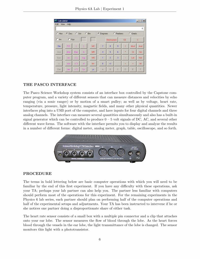
THE PASCO INTERFACE
The Pasco Science Workshop system consists of an interface box controlled by the Capstone com-puter program, and a variety of different sensors that can measure distances and velocities by echoranging (via a sonic ranger) or by motion of a smart pulley; as well as by voltage, heart rate,temperature, pressure, light intensity, magnetic fields, and many other physical quantities. Newerinterfaces plug into a USB port of the computer, and have inputs for four digital channels and threeanalog channels. The interface can measure several quantities simultaneously and also has a built-insignal generator which can be controlled to produce 0 – 5 volt signals of DC, AC, and several otherdifferent wave forms. The software with the interface permits you to display and analyze the resultsin a number of different forms: digital meter, analog meter, graph, table, oscilloscope, and so forth.
PROCEDURE
The terms in bold lettering below are basic computer operations with which you will need to befamiliar by the end of this first experiment. If you have any difficulty with these operations, askyour TA; perhaps your lab partner can also help you. The partner less familiar with computersshould perform most of the operations for this experiment. For the remaining experiments in thePhysics 6 lab series, each partner should plan on performing half of the computer operations andhalf of the experimental setups and adjustments. Your TA has been instructed to intervene if he orshe notices one partner doing a disproportionate share of either task.
The heart rate sensor consists of a small box with a multiple pin connector and a clip that attachesonto your ear lobe. The sensor measures the flow of blood through the lobe. As the heart forcesblood through the vessels in the ear lobe, the light transmittance of the lobe is changed. The sensormonitors this light with a phototransistor.
6
Physics 6A Lab | Experiment 1
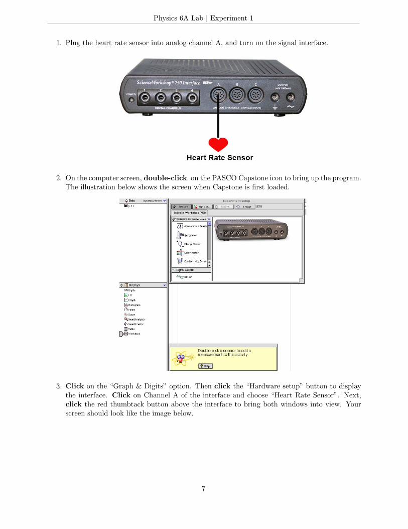
1. Plug the heart rate sensor into analog channel A, and turn on the signal interface.
2. On the computer screen, double-click on the PASCO Capstone icon to bring up the program.The illustration below shows the screen when Capstone is first loaded.
3. Click on the “Graph & Digits” option. Then click the “Hardware setup” button to displaythe interface. Click on Channel A of the interface and choose “Heart Rate Sensor”. Next,click the red thumbtack button above the interface to bring both windows into view. Yourscreen should look like the image below.
7
Physics 6A Lab | Experiment 1
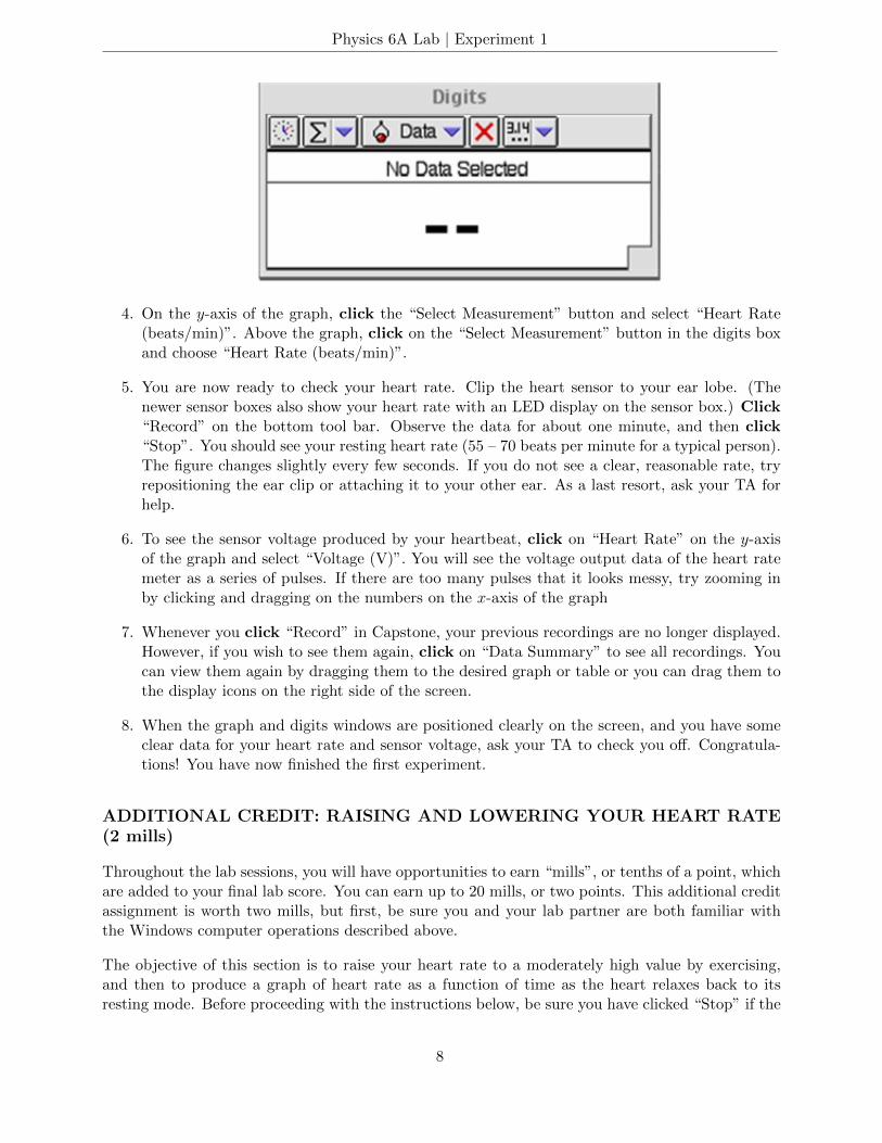
4. On the y-axis of the graph, click the “Select Measurement” button and select “Heart Rate(beats/min)”. Above the graph, click on the “Select Measurement” button in the digits boxand choose “Heart Rate (beats/min)”.
5. You are now ready to check your heart rate. Clip the heart sensor to your ear lobe. (Thenewer sensor boxes also show your heart rate with an LED display on the sensor box.) Click“Record” on the bottom tool bar. Observe the data for about one minute, and then click“Stop”. You should see your resting heart rate (55 – 70 beats per minute for a typical person).The figure changes slightly every few seconds. If you do not see a clear, reasonable rate, tryrepositioning the ear clip or attaching it to your other ear. As a last resort, ask your TA forhelp.
6. To see the sensor voltage produced by your heartbeat, click on “Heart Rate” on the y-axisof the graph and select “Voltage (V)”. You will see the voltage output data of the heart ratemeter as a series of pulses. If there are too many pulses that it looks messy, try zooming inby clicking and dragging on the numbers on the x-axis of the graph
7. Whenever you click “Record” in Capstone, your previous recordings are no longer displayed.However, if you wish to see them again, click on “Data Summary” to see all recordings. Youcan view them again by dragging them to the desired graph or table or you can drag them tothe display icons on the right side of the screen.
8. When the graph and digits windows are positioned clearly on the screen, and you have someclear data for your heart rate and sensor voltage, ask your TA to check you off. Congratula-tions! You have now finished the first experiment.
ADDITIONAL CREDIT: RAISING AND LOWERING YOUR HEART RATE(2 mills)
Throughout the lab sessions, you will have opportunities to earn “mills”, or tenths of a point, whichare added to your final lab score. You can earn up to 20 mills, or two points. This additional creditassignment is worth two mills, but first, be sure you and your lab partner are both familiar withthe Windows computer operations described above.
The objective of this section is to raise your heart rate to a moderately high value by exercising,and then to produce a graph of heart rate as a function of time as the heart relaxes back to itsresting mode. Before proceeding with the instructions below, be sure you have clicked “Stop” if the
8
Physics 6A Lab | Experiment 1
machine is still monitoring your heartbeat.
The sensor will not record an accurate heart rate when you are moving around. You will need totake off the sensor, exercise, and then hook yourself back up. Raise your heart rate to 140 beatsper minute or higher by doing jumping jacks in position, or by going out and running around thebuilding. Do not perform the exercise if you have a health problem. Have your lab partner oranother volunteer do it. After exercising, reattach the sensor, and click “Record” to record yourheart rate as a function of time. Remain as still as possible while the recording is made — say, forfive minutes (or 300 seconds). Click “Stop” when you are finished.
Your graph should show a relatively smooth, decreasing heart rate from 140 beats per minute downtoward your resting rate. If you do not obtain a smooth graph, get some more exercise and tryagain. Try to remain more still while recording, reposition the ear clip, or attach it to your otherear until you get a nice result. If the appearance of the graph is satisfactory, you can show thisgraph to your TA to collect two mills.
9
Physics 6A Lab | Experiment 2
Kinematics
APPARATUS
• Computer and Pasco interface
• Motion sensor (sonic ranger)
• Air track, glider with reflector, block to tilt track
• Calipers to measure thickness of block
• Pendulum arrangement
INTRODUCTION
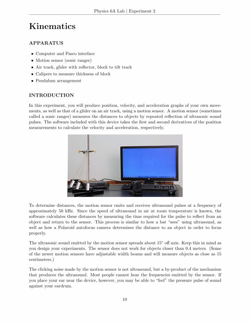
In this experiment, you will produce position, velocity, and acceleration graphs of your own move-ments, as well as that of a glider on an air track, using a motion sensor. A motion sensor (sometimescalled a sonic ranger) measures the distances to objects by repeated reflection of ultrasonic soundpulses. The software included with this device takes the first and second derivatives of the positionmeasurements to calculate the velocity and acceleration, respectively.
To determine distances, the motion sensor emits and receives ultrasound pulses at a frequency ofapproximately 50 kHz. Since the speed of ultrasound in air at room temperature is known, thesoftware calculates these distances by measuring the time required for the pulse to reflect from anobject and return to the sensor. This process is similar to how a bat “sees” using ultrasound, aswell as how a Polaroid autofocus camera determines the distance to an object in order to focusproperly.
The ultrasonic sound emitted by the motion sensor spreads about 15 off axis. Keep this in mind asyou design your experiments. The sensor does not work for objects closer than 0.4 meters. (Someof the newer motion sensors have adjustable width beams and will measure objects as close as 15centimeters.)
The clicking noise made by the motion sensor is not ultrasound, but a by-product of the mechanismthat produces the ultrasound. Most people cannot hear the frequencies emitted by the sensor. Ifyou place your ear near the device, however, you may be able to “feel” the pressure pulse of soundagainst your eardrum.
10
Physics 6A Lab | Experiment 2
INITIAL SETUP
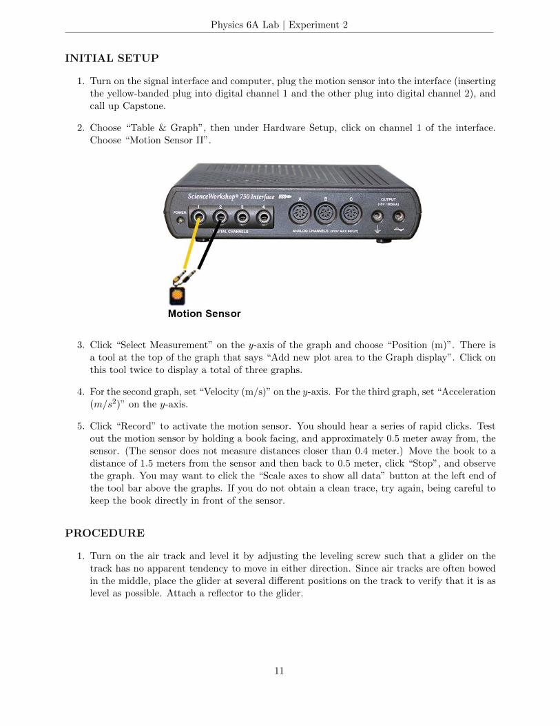
1. Turn on the signal interface and computer, plug the motion sensor into the interface (insertingthe yellow-banded plug into digital channel 1 and the other plug into digital channel 2), andcall up Capstone.
2. Choose “Table & Graph”, then under Hardware Setup, click on channel 1 of the interface.Choose “Motion Sensor II”.
3. Click “Select Measurement” on the y-axis of the graph and choose “Position (m)”. There isa tool at the top of the graph that says “Add new plot area to the Graph display”. Click onthis tool twice to display a total of three graphs.
4. For the second graph, set “Velocity (m/s)” on the y-axis. For the third graph, set “Acceleration(m/s2)” on the y-axis.
5. Click “Record” to activate the motion sensor. You should hear a series of rapid clicks. Testout the motion sensor by holding a book facing, and approximately 0.5 meter away from, thesensor. (The sensor does not measure distances closer than 0.4 meter.) Move the book to adistance of 1.5 meters from the sensor and then back to 0.5 meter, click “Stop”, and observethe graph. You may want to click the “Scale axes to show all data” button at the left end ofthe tool bar above the graphs. If you do not obtain a clean trace, try again, being careful tokeep the book directly in front of the sensor.
PROCEDURE
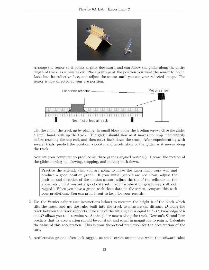
1. Turn on the air track and level it by adjusting the leveling screw such that a glider on thetrack has no apparent tendency to move in either direction. Since air tracks are often bowedin the middle, place the glider at several different positions on the track to verify that it is aslevel as possible. Attach a reflector to the glider.
11
Physics 6A Lab | Experiment 2
Arrange the sensor so it points slightly downward and can follow the glider along the entirelength of track, as shown below. Place your eye at the position you want the sensor to point.Look into its reflective face, and adjust the sensor until you see your reflected image. Thesensor is now directed at your eye position.
Tilt the end of the track up by placing the small block under the leveling screw. Give the glidera small hand push up the track. The glider should slow as it moves up, stop momentarilybefore reaching the top end, and then coast back down the track. After experimenting withseveral trials, predict the position, velocity, and acceleration of the glider as it moves alongthe track.
Now set your computer to produce all three graphs aligned vertically. Record the motion ofthe glider moving up, slowing, stopping, and moving back down.
Practice the attitude that you are going to make the experiment work well andproduce a good position graph. If your initial graphs are not clean, adjust theposition and direction of the motion sensor, adjust the tilt of the reflector on theglider, etc., until you get a good data set. (Your acceleration graph may still lookragged.) When you have a graph with clean data on the screen, compare this withyour predictions. You can print it out to keep for your records.
2. Use the Vernier caliper (see instructions below) to measure the height h of the block whichtilts the track, and use the ruler built into the track to measure the distance D along thetrack between the track supports. The sine of the tilt angle α is equal to h/D; knowledge of hand D allows you to determine α. As the glider moves along the track, Newton’s Second Lawpredicts that its acceleration should be constant and equal in magnitude to g sinα. Calculatethe value of this acceleration. This is your theoretical prediction for the acceleration of thecart.
3. Acceleration graphs often look ragged, as small errors accumulate when the software takes
12
Physics 6A Lab | Experiment 2
the second derivative of the position data. We will use the method of linear regression todetermine the the acceleration of the cart. Notice the linearly increasing portion of yourvelocity graph. Select this region of interest by first clicking on the velocity graph thenclicking on the “Highlight range of points in active data” tool. A rectangle will appear. Dragand extend this rectangle over the linearly increasing portion of your data. Click inside therectangle to highlight the data.
4. Click the drop-down arrow of the “Apply selected curve fits to active...” tool and choose“Linear”. Click this tool again to bring up a display box. You should see a best-fit line appearon top your selected data and a box should pop up that tells you the slope and y-interceptof this best-fit line. The slope of this line is your experimentally measured acceleration of thecart. Write this value down for your analysis.
5. Another way to measure the acceleration is by looking at the acceleration graph. In generalyour graph should be flat (and possibly a a bit ragged). We want to find the average of thesedata points. To do this, select the data points of interest using the “Highlight range of pointsin active data” tool. Click the “Display selected statistics for active...” tool. This will displaythe mean value of the points you selected. Compare this to the value you obtained by makinga best-fit line.
Note: By default, Capstone gives only one digit of precision for acceleration measurements andcalculations performed using them. You can increase this precision as follows: Open “DataSummary” from the left hand panel and select the name of the measurement in question. Inthis case, you would select “Acceleration (m/s2)” . Next click the blue gear icon (settings),open the “Numerical Format” dropdown menu, and modify the “Number of Decimal Places”as desired.
6. Calculate the percentage error between the experimental results aexp obtained in steps 4 and5, and the theoretical value ath determined in step 2:
percentage error = (100%)× (| aexp − ath |) /ath.
The absolute value is taken because we are not interested in the sign of the difference. Typicalexperimental accuracies in an undergraduate lab range from 3 – 5%, although some quantitiescan be measured much more accurately (and some much less!).
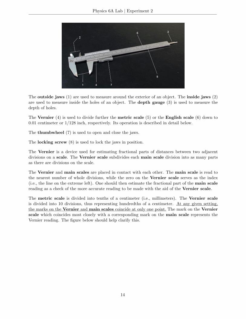
VERNIER CALIPER
The Vernier caliper is designed to provide a highly precise measurement of length. The numbersin parentheses refer to those found in the figure below.
13
Physics 6A Lab | Experiment 2
The outside jaws (1) are used to measure around the exterior of an object. The inside jaws (2)are used to measure inside the holes of an object. The depth gauge (3) is used to measure thedepth of holes.
The Vernier (4) is used to divide further the metric scale (5) or the English scale (6) down to0.01 centimeter or 1/128 inch, respectively. Its operation is described in detail below.
The thumbwheel (7) is used to open and close the jaws.
The locking screw (8) is used to lock the jaws in position.
The Vernier is a device used for estimating fractional parts of distances between two adjacentdivisions on a scale. The Vernier scale subdivides each main scale division into as many partsas there are divisions on the scale.
The Vernier and main scales are placed in contact with each other. The main scale is read tothe nearest number of whole divisions, while the zero on the Vernier scale serves as the index(i.e., the line on the extreme left). One should then estimate the fractional part of the main scalereading as a check of the more accurate reading to be made with the aid of the Vernier scale.
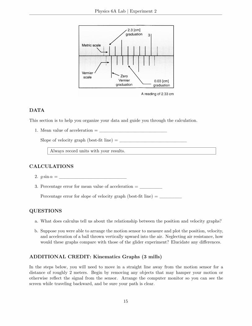
The metric scale is divided into tenths of a centimeter (i.e., millimeters). The Vernier scaleis divided into 10 divisions, thus representing hundredths of a centimeter. At any given setting,the marks on the Vernier and main scales coincide at only one point. The mark on the Vernierscale which coincides most closely with a corresponding mark on the main scale represents theVernier reading. The figure below should help clarify this.
14
Physics 6A Lab | Experiment 2
DATA
This section is to help you organize your data and guide you through the calculation.
1. Mean value of acceleration =
Slope of velocity graph (best-fit line) =
Always record units with your results.
CALCULATIONS
2. g sinα =
3. Percentage error for mean value of acceleration =
Percentage error for slope of velocity graph (best-fit line) =
QUESTIONS
a. What does calculus tell us about the relationship between the position and velocity graphs?
b. Suppose you were able to arrange the motion sensor to measure and plot the position, velocity,and acceleration of a ball thrown vertically upward into the air. Neglecting air resistance, howwould these graphs compare with those of the glider experiment? Elucidate any differences.
ADDITIONAL CREDIT: Kinematics Graphs (3 mills)
In the steps below, you will need to move in a straight line away from the motion sensor for adistance of roughly 2 meters. Begin by removing any objects that may hamper your motion orotherwise reflect the signal from the sensor. Arrange the computer monitor so you can see thescreen while traveling backward, and be sure your path is clear.
15
Physics 6A Lab | Experiment 2
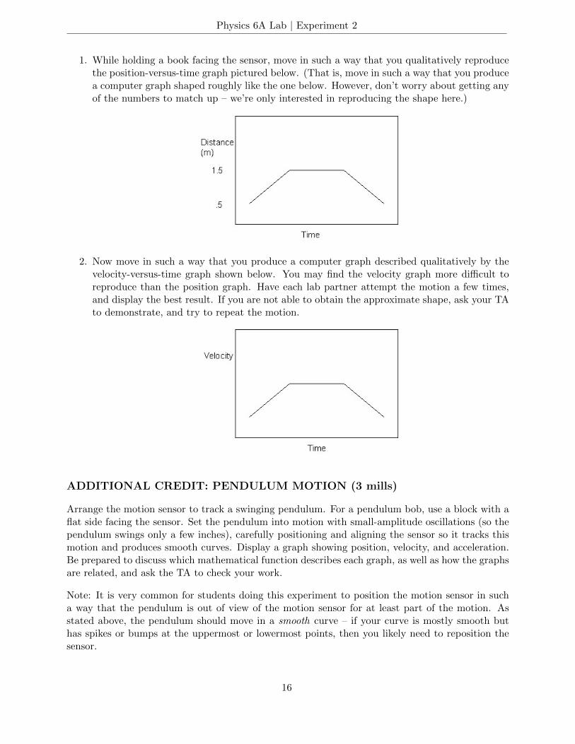
1. While holding a book facing the sensor, move in such a way that you qualitatively reproducethe position-versus-time graph pictured below. (That is, move in such a way that you producea computer graph shaped roughly like the one below. However, don’t worry about getting anyof the numbers to match up – we’re only interested in reproducing the shape here.)
2. Now move in such a way that you produce a computer graph described qualitatively by thevelocity-versus-time graph shown below. You may find the velocity graph more difficult toreproduce than the position graph. Have each lab partner attempt the motion a few times,and display the best result. If you are not able to obtain the approximate shape, ask your TAto demonstrate, and try to repeat the motion.
ADDITIONAL CREDIT: PENDULUM MOTION (3 mills)
Arrange the motion sensor to track a swinging pendulum. For a pendulum bob, use a block with aflat side facing the sensor. Set the pendulum into motion with small-amplitude oscillations (so thependulum swings only a few inches), carefully positioning and aligning the sensor so it tracks thismotion and produces smooth curves. Display a graph showing position, velocity, and acceleration.Be prepared to discuss which mathematical function describes each graph, as well as how the graphsare related, and ask the TA to check your work.
Note: It is very common for students doing this experiment to position the motion sensor in sucha way that the pendulum is out of view of the motion sensor for at least part of the motion. Asstated above, the pendulum should move in a smooth curve – if your curve is mostly smooth buthas spikes or bumps at the uppermost or lowermost points, then you likely need to reposition thesensor.
16
Physics 6A Lab | Experiment 3
Newton’s Second Law
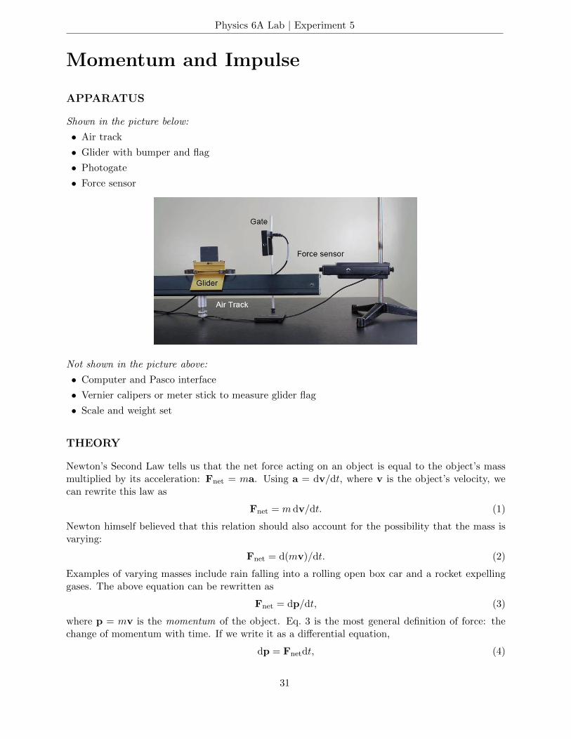
APPARATUS
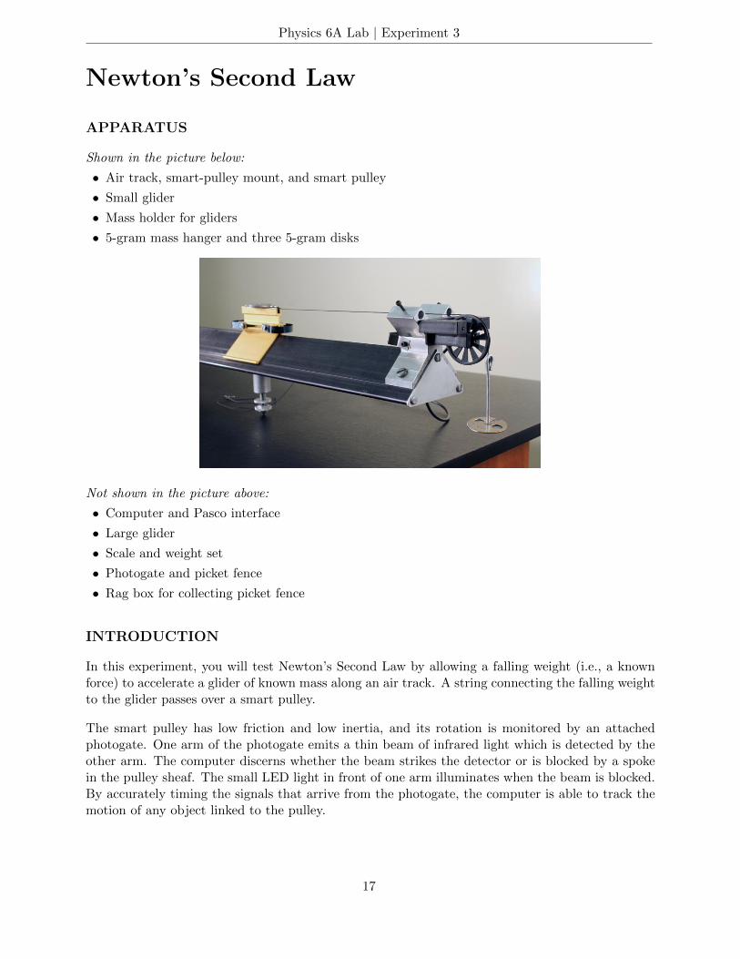
Shown in the picture below:
• Air track, smart-pulley mount, and smart pulley
• Small glider
• Mass holder for gliders
• 5-gram mass hanger and three 5-gram disks
Not shown in the picture above:
• Computer and Pasco interface
• Large glider
• Scale and weight set
• Photogate and picket fence
• Rag box for collecting picket fence
INTRODUCTION
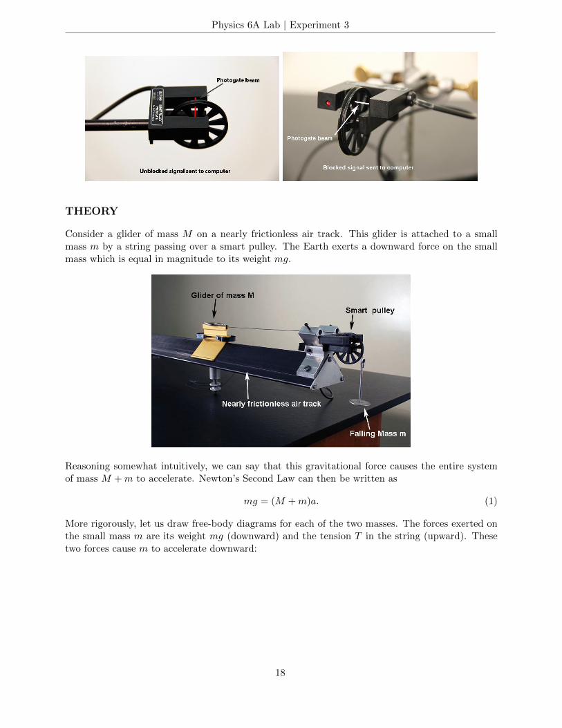
In this experiment, you will test Newton’s Second Law by allowing a falling weight (i.e., a knownforce) to accelerate a glider of known mass along an air track. A string connecting the falling weightto the glider passes over a smart pulley.
The smart pulley has low friction and low inertia, and its rotation is monitored by an attachedphotogate. One arm of the photogate emits a thin beam of infrared light which is detected by theother arm. The computer discerns whether the beam strikes the detector or is blocked by a spokein the pulley sheaf. The small LED light in front of one arm illuminates when the beam is blocked.By accurately timing the signals that arrive from the photogate, the computer is able to track themotion of any object linked to the pulley.
17
Physics 6A Lab | Experiment 3
THEORY
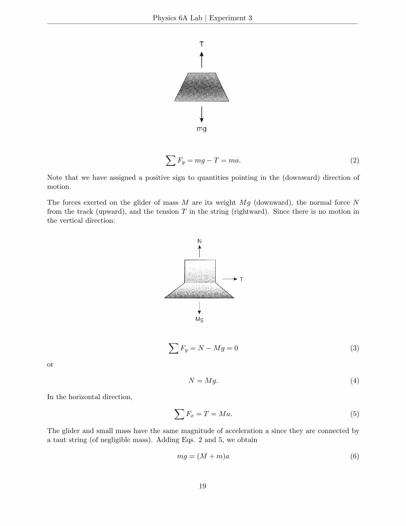
Consider a glider of mass M on a nearly frictionless air track. This glider is attached to a smallmass m by a string passing over a smart pulley. The Earth exerts a downward force on the smallmass which is equal in magnitude to its weight mg.
Reasoning somewhat intuitively, we can say that this gravitational force causes the entire systemof mass M +m to accelerate. Newton’s Second Law can then be written as
mg = (M +m)a. (1)
More rigorously, let us draw free-body diagrams for each of the two masses. The forces exerted onthe small mass m are its weight mg (downward) and the tension T in the string (upward). Thesetwo forces cause m to accelerate downward:
18
Physics 6A Lab | Experiment 3
∑Fy = mg − T = ma. (2)
Note that we have assigned a positive sign to quantities pointing in the (downward) direction ofmotion.
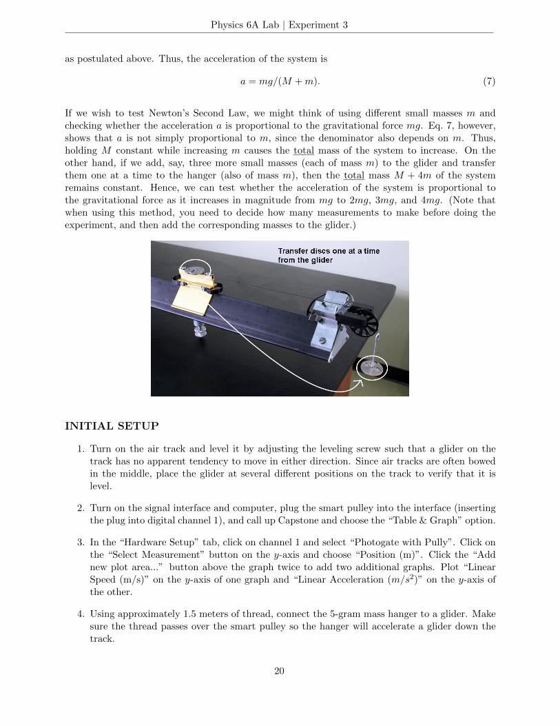
The forces exerted on the glider of mass M are its weight Mg (downward), the normal force Nfrom the track (upward), and the tension T in the string (rightward). Since there is no motion inthe vertical direction:
∑Fy = N −Mg = 0 (3)
or
N = Mg. (4)
In the horizontal direction, ∑Fx = T = Ma. (5)
The glider and small mass have the same magnitude of acceleration a since they are connected bya taut string (of negligible mass). Adding Eqs. 2 and 5, we obtain
mg = (M +m)a (6)
19
Physics 6A Lab | Experiment 3
as postulated above. Thus, the acceleration of the system is
a = mg/(M +m). (7)
If we wish to test Newton’s Second Law, we might think of using different small masses m andchecking whether the acceleration a is proportional to the gravitational force mg. Eq. 7, however,shows that a is not simply proportional to m, since the denominator also depends on m. Thus,holding M constant while increasing m causes the total mass of the system to increase. On theother hand, if we add, say, three more small masses (each of mass m) to the glider and transferthem one at a time to the hanger (also of mass m), then the total mass M + 4m of the systemremains constant. Hence, we can test whether the acceleration of the system is proportional tothe gravitational force as it increases in magnitude from mg to 2mg, 3mg, and 4mg. (Note thatwhen using this method, you need to decide how many measurements to make before doing theexperiment, and then add the corresponding masses to the glider.)
INITIAL SETUP
1. Turn on the air track and level it by adjusting the leveling screw such that a glider on thetrack has no apparent tendency to move in either direction. Since air tracks are often bowedin the middle, place the glider at several different positions on the track to verify that it islevel.
2. Turn on the signal interface and computer, plug the smart pulley into the interface (insertingthe plug into digital channel 1), and call up Capstone and choose the “Table & Graph” option.
3. In the “Hardware Setup” tab, click on channel 1 and select “Photogate with Pully”. Click onthe “Select Measurement” button on the y-axis and choose “Position (m)”. Click the “Addnew plot area...” button above the graph twice to add two additional graphs. Plot “LinearSpeed (m/s)” on the y-axis of one graph and “Linear Acceleration (m/s2)” on the y-axis ofthe other.
4. Using approximately 1.5 meters of thread, connect the 5-gram mass hanger to a glider. Makesure the thread passes over the smart pulley so the hanger will accelerate a glider down thetrack.
20
Physics 6A Lab | Experiment 3
PROCEDURE
1. Weigh each glider to obtain its mass, and record the values in the “Data” section.
2. Attach (or tape) three 5-gram masses to the small glider, such that only the 5-gram massholder accelerates the glider. Turn the air-track blower on, and set one glider on the track asfar from the pulley as the thread allows. Click “Record”, and immediately release the gliderso that it begins to move. Just before the hanger hits the floor or the glider reaches the endof the track, click “Stop”.
3. Check the graph window and use the “Scale-to-fit” button, if necessary. Check that you areobtaining reasonable plots of the glider’s position, velocity, and acceleration. As usual, theacceleration graph may look ragged.
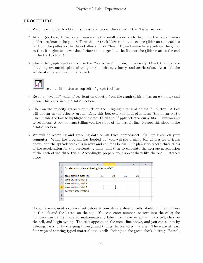
scale-to-fit button at top left of graph tool bar
4. Read an “eyeball” value of acceleration directly from the graph (This is just an estimate) andrecord this value in the “Data” section.
5. Click on the velocity graph then click on the “Highlight rang of points...” button. A boxwill appear in the velocity graph. Drag this box over the data of interest (the linear part).Click inside the box to highlight the data. Click the “Apply selected curve fits...” button andselect linear. A box appears telling you the slope of the best-fit line. Record this slope in the“Data” section.
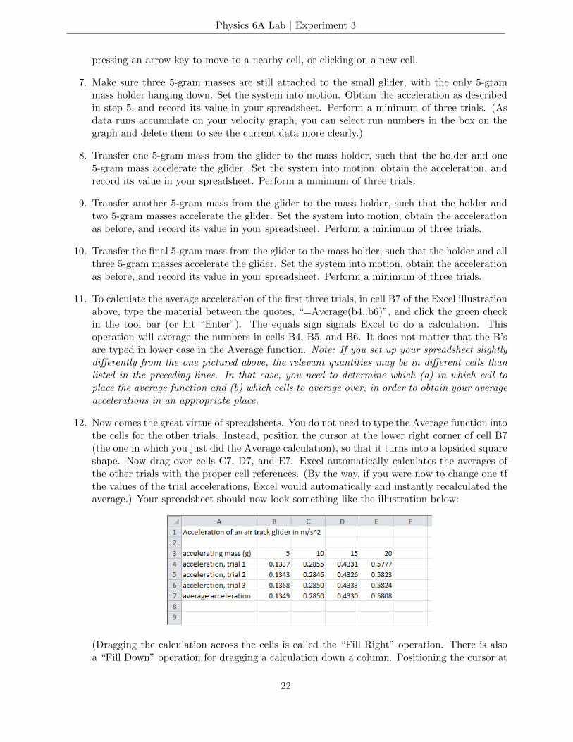
6. We will be recording and graphing data on an Excel spreadsheet. Call up Excel on yourcomputer. When the program has booted up, you will see a menu bar with a set of iconsabove, and the spreadsheet cells in rows and columns below. Our plan is to record three trialsof the acceleration for the accelerating mass, and then to calculate the average accelerationof the each of the three trials. Accordingly, prepare your spreadsheet like the one illustratedbelow.
If you have not used a spreadsheet before, it consists of a sheet of cells labeled by the numberson the left and the letters on the top. You can enter numbers or text into the cells; thenumbers can be manipulated mathematically later. To make an entry into a cell, click onthe cell, and begin typing. The text appears on the menu line above, and you can edit it bydeleting parts, or by dragging through and typing the corrected material. There are at leastfour ways of entering typed material into a cell: clicking on the green check, hitting “Enter”,
21
Physics 6A Lab | Experiment 3
pressing an arrow key to move to a nearby cell, or clicking on a new cell.
7. Make sure three 5-gram masses are still attached to the small glider, with the only 5-grammass holder hanging down. Set the system into motion. Obtain the acceleration as describedin step 5, and record its value in your spreadsheet. Perform a minimum of three trials. (Asdata runs accumulate on your velocity graph, you can select run numbers in the box on thegraph and delete them to see the current data more clearly.)
8. Transfer one 5-gram mass from the glider to the mass holder, such that the holder and one5-gram mass accelerate the glider. Set the system into motion, obtain the acceleration, andrecord its value in your spreadsheet. Perform a minimum of three trials.
9. Transfer another 5-gram mass from the glider to the mass holder, such that the holder andtwo 5-gram masses accelerate the glider. Set the system into motion, obtain the accelerationas before, and record its value in your spreadsheet. Perform a minimum of three trials.
10. Transfer the final 5-gram mass from the glider to the mass holder, such that the holder and allthree 5-gram masses accelerate the glider. Set the system into motion, obtain the accelerationas before, and record its value in your spreadsheet. Perform a minimum of three trials.
11. To calculate the average acceleration of the first three trials, in cell B7 of the Excel illustrationabove, type the material between the quotes, “=Average(b4..b6)”, and click the green checkin the tool bar (or hit “Enter”). The equals sign signals Excel to do a calculation. Thisoperation will average the numbers in cells B4, B5, and B6. It does not matter that the B’sare typed in lower case in the Average function. Note: If you set up your spreadsheet slightlydifferently from the one pictured above, the relevant quantities may be in different cells thanlisted in the preceding lines. In that case, you need to determine which (a) in which cell toplace the average function and (b) which cells to average over, in order to obtain your averageaccelerations in an appropriate place.
12. Now comes the great virtue of spreadsheets. You do not need to type the Average function intothe cells for the other trials. Instead, position the cursor at the lower right corner of cell B7(the one in which you just did the Average calculation), so that it turns into a lopsided squareshape. Now drag over cells C7, D7, and E7. Excel automatically calculates the averages ofthe other trials with the proper cell references. (By the way, if you were now to change one tfthe values of the trial accelerations, Excel would automatically and instantly recalculated theaverage.) Your spreadsheet should now look something like the illustration below:
(Dragging the calculation across the cells is called the “Fill Right” operation. There is alsoa “Fill Down” operation for dragging a calculation down a column. Positioning the cursor at
22
Physics 6A Lab | Experiment 3
the corner of the cell is a short cut to these operations. They can also be accessed from the“Edit” pull down menu.)
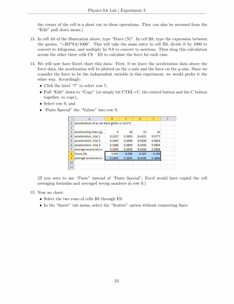
13. In cell A8 of the illustration above, type “Force (N)”. In cell B8, type the expression betweenthe quotes, “=B3*9.8/1000”. This will take the mass entry in cell B3, divide it by 1000 toconvert to kilograms, and multiply by 9.8 to convert to newtons. Then drag this calculationacross the other three cells C8 – E8 to calculate the force for each case.
14. We will now have Excel chart this data. First, if we leave the acceleration data above theforce data, the acceleration will be plotted on the x-axis and the force on the y-axis. Since weconsider the force to be the independent variable in this experiment, we would prefer it theother way. Accordingly:
• Click the label “7” to select row 7,
• Pull “Edit” down to “Copy” (or simply hit CTRL+C, the control button and the C buttontogether, to copy),
• Select row 9, and
• “Paste Special” the “Values” into row 9.
(If you were to use “Paste” instead of “Paste Special”, Excel would have copied the cellaveraging formulas and averaged wrong numbers in row 9.)
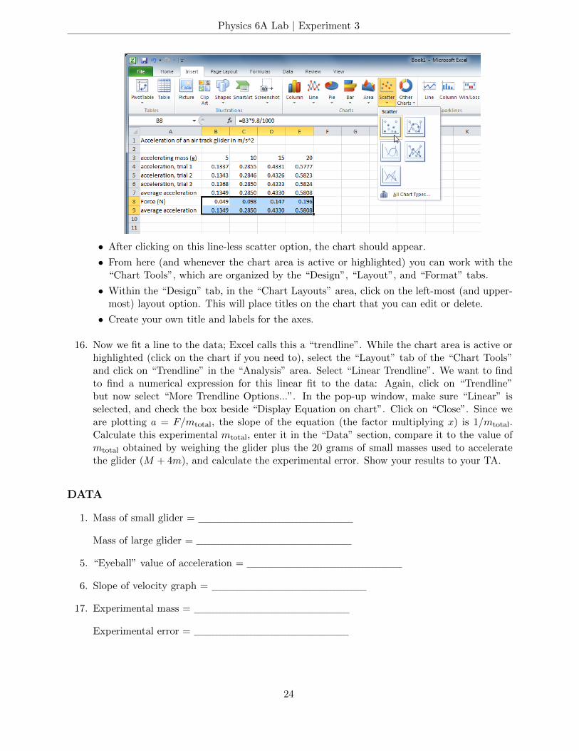
15. Now we chart:
• Select the two rows of cells B8 through E9.
• In the “Insert” tab menu, select the “Scatter” option without connecting lines:
23
Physics 6A Lab | Experiment 3
• After clicking on this line-less scatter option, the chart should appear.
• From here (and whenever the chart area is active or highlighted) you can work with the“Chart Tools”, which are organized by the “Design”, “Layout”, and “Format” tabs.
• Within the “Design” tab, in the “Chart Layouts” area, click on the left-most (and upper-most) layout option. This will place titles on the chart that you can edit or delete.
• Create your own title and labels for the axes.
16. Now we fit a line to the data; Excel calls this a “trendline”. While the chart area is active orhighlighted (click on the chart if you need to), select the “Layout” tab of the “Chart Tools”and click on “Trendline” in the “Analysis” area. Select “Linear Trendline”. We want to findto find a numerical expression for this linear fit to the data: Again, click on “Trendline”but now select “More Trendline Options...”. In the pop-up window, make sure “Linear” isselected, and check the box beside “Display Equation on chart”. Click on “Close”. Since weare plotting a = F/mtotal, the slope of the equation (the factor multiplying x) is 1/mtotal.Calculate this experimental mtotal, enter it in the “Data” section, compare it to the value ofmtotal obtained by weighing the glider plus the 20 grams of small masses used to acceleratethe glider (M + 4m), and calculate the experimental error. Show your results to your TA.
DATA
1. Mass of small glider =
Mass of large glider =
5. “Eyeball” value of acceleration =
6. Slope of velocity graph =
17. Experimental mass =
Experimental error =
24
Physics 6A Lab | Experiment 3
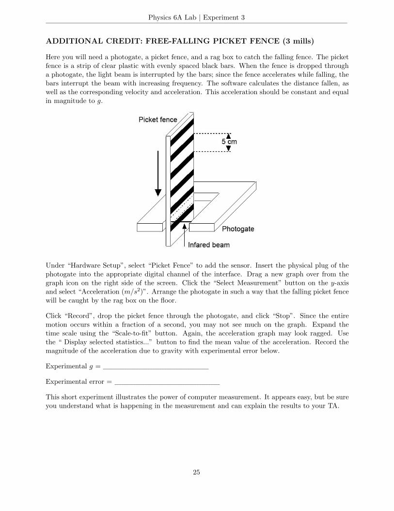
ADDITIONAL CREDIT: FREE-FALLING PICKET FENCE (3 mills)
Here you will need a photogate, a picket fence, and a rag box to catch the falling fence. The picketfence is a strip of clear plastic with evenly spaced black bars. When the fence is dropped througha photogate, the light beam is interrupted by the bars; since the fence accelerates while falling, thebars interrupt the beam with increasing frequency. The software calculates the distance fallen, aswell as the corresponding velocity and acceleration. This acceleration should be constant and equalin magnitude to g.
Under “Hardware Setup”, select “Picket Fence” to add the sensor. Insert the physical plug of thephotogate into the appropriate digital channel of the interface. Drag a new graph over from thegraph icon on the right side of the screen. Click the “Select Measurement” button on the y-axisand select “Acceleration (m/s2)”. Arrange the photogate in such a way that the falling picket fencewill be caught by the rag box on the floor.
Click “Record”, drop the picket fence through the photogate, and click “Stop”. Since the entiremotion occurs within a fraction of a second, you may not see much on the graph. Expand thetime scale using the “Scale-to-fit” button. Again, the acceleration graph may look ragged. Usethe “ Display selected statistics...” button to find the mean value of the acceleration. Record themagnitude of the acceleration due to gravity with experimental error below.
Experimental g =
Experimental error =
This short experiment illustrates the power of computer measurement. It appears easy, but be sureyou understand what is happening in the measurement and can explain the results to your TA.
25
Physics 6A Lab | Experiment 4
Conservation of Energy
APPARATUS
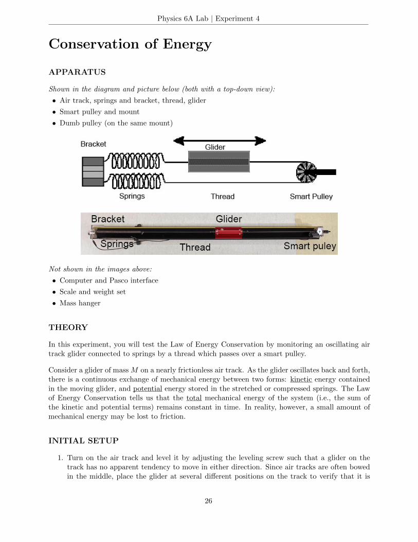
Shown in the diagram and picture below (both with a top-down view):
• Air track, springs and bracket, thread, glider
• Smart pulley and mount
• Dumb pulley (on the same mount)
Not shown in the images above:
• Computer and Pasco interface
• Scale and weight set
• Mass hanger
THEORY
In this experiment, you will test the Law of Energy Conservation by monitoring an oscillating airtrack glider connected to springs by a thread which passes over a smart pulley.
Consider a glider of mass M on a nearly frictionless air track. As the glider oscillates back and forth,there is a continuous exchange of mechanical energy between two forms: kinetic energy containedin the moving glider, and potential energy stored in the stretched or compressed springs. The Lawof Energy Conservation tells us that the total mechanical energy of the system (i.e., the sum ofthe kinetic and potential terms) remains constant in time. In reality, however, a small amount ofmechanical energy may be lost to friction.
INITIAL SETUP
1. Turn on the air track and level it by adjusting the leveling screw such that a glider on thetrack has no apparent tendency to move in either direction. Since air tracks are often bowedin the middle, place the glider at several different positions on the track to verify that it is
26
Physics 6A Lab | Experiment 4
level.
2. Weigh the glider to obtain its mass, and record this value in the “Data” section.
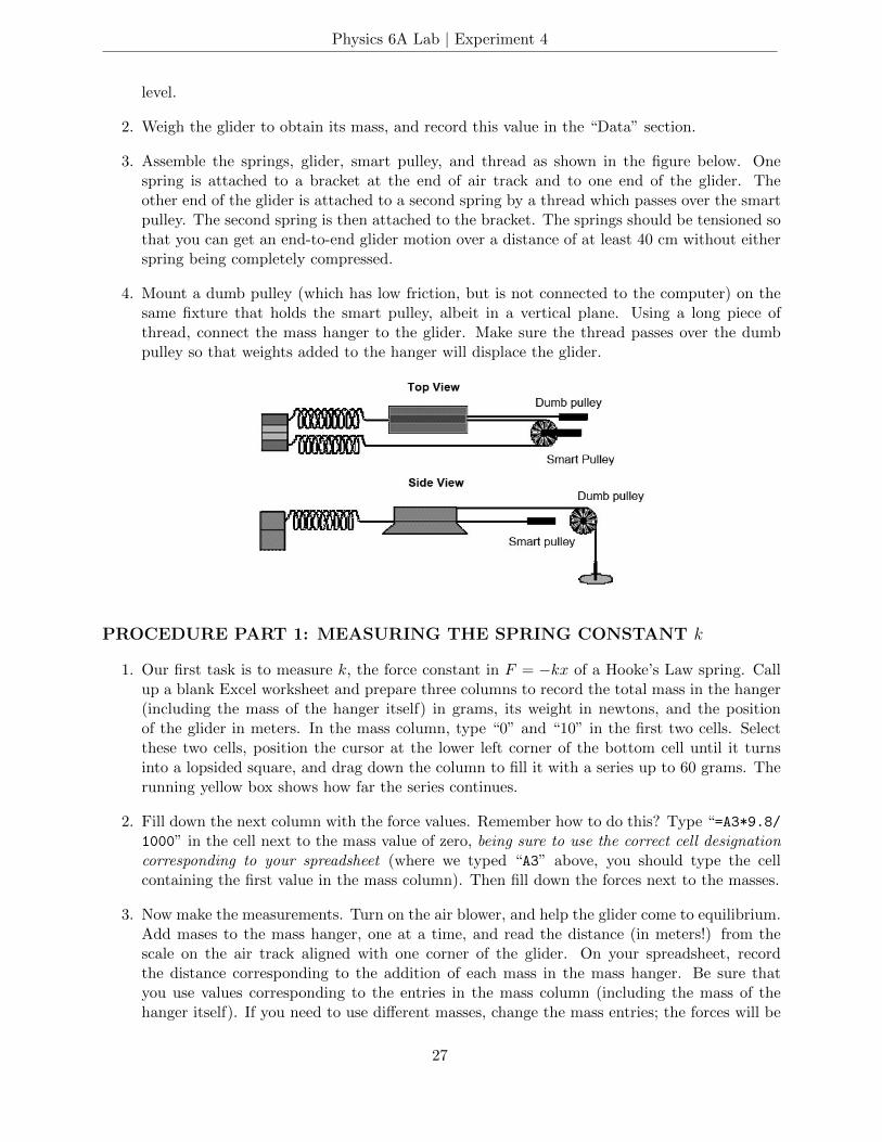
3. Assemble the springs, glider, smart pulley, and thread as shown in the figure below. Onespring is attached to a bracket at the end of air track and to one end of the glider. Theother end of the glider is attached to a second spring by a thread which passes over the smartpulley. The second spring is then attached to the bracket. The springs should be tensioned sothat you can get an end-to-end glider motion over a distance of at least 40 cm without eitherspring being completely compressed.
4. Mount a dumb pulley (which has low friction, but is not connected to the computer) on thesame fixture that holds the smart pulley, albeit in a vertical plane. Using a long piece ofthread, connect the mass hanger to the glider. Make sure the thread passes over the dumbpulley so that weights added to the hanger will displace the glider.
PROCEDURE PART 1: MEASURING THE SPRING CONSTANT k
1. Our first task is to measure k, the force constant in F = −kx of a Hooke’s Law spring. Callup a blank Excel worksheet and prepare three columns to record the total mass in the hanger(including the mass of the hanger itself) in grams, its weight in newtons, and the positionof the glider in meters. In the mass column, type “0” and “10” in the first two cells. Selectthese two cells, position the cursor at the lower left corner of the bottom cell until it turnsinto a lopsided square, and drag down the column to fill it with a series up to 60 grams. Therunning yellow box shows how far the series continues.
2. Fill down the next column with the force values. Remember how to do this? Type “=A3*9.8/1000” in the cell next to the mass value of zero, being sure to use the correct cell designationcorresponding to your spreadsheet (where we typed “A3” above, you should type the cellcontaining the first value in the mass column). Then fill down the forces next to the masses.
3. Now make the measurements. Turn on the air blower, and help the glider come to equilibrium.Add mases to the mass hanger, one at a time, and read the distance (in meters!) from thescale on the air track aligned with one corner of the glider. On your spreadsheet, recordthe distance corresponding to the addition of each mass in the mass hanger. Be sure thatyou use values corresponding to the entries in the mass column (including the mass of thehanger itself). If you need to use different masses, change the mass entries; the forces will be
27
Physics 6A Lab | Experiment 4
recalculated instantly.
4. When you have filled in the distance column next to the force column, chart these variablesagainst each other in Excel, and find the slope. Here is a reminder of how this is done:
• Select the cells with numbers in the force and distance columns.
• In the “Insert” tab menu, select the “Scatter” option without connecting lines. Afterclicking on this line-less scatter option, the chart should appear.
• Within the “Design” tab of the “Chart Tools”, in the “Chart Layouts” area, click on theleft-most (and upper-most) layout option. This will place titles on the chart that you canedit or delete.
• Create your own title and labels for the axes.
• In the “Layout” tab of the “Chart Tools”, click on “Trendline” in the “Analysis” area.Select “More Trendline Options...”. In the pop-up window, make sure “Linear” is selected,and check the box beside “Display Equation on chart”. Click on “Close”.
Convince yourself that the slope is 1/k and not k. Record the value of k in the “Data” section.
PROCEDURE PART 2: PLOTTING ENERGIES
1. Unhook the mass hanger string. Hook up the smart pulley physically and virtually, in Cap-stone (the sensor is called “Photogate with Pulley”). Choose the “Table & Graph” option inCapstone. Choose “Position (m)” for the y-axis of the graph. Add another graph by clickingthe “Add new plot area...” button. On this new graph, select “Linear Speed (m/s)” for they-axis. Add a third graph and plot “Linear Acceleration (m/s2) on the y-axis.
2. With the air blower on, pull the glider out, click “Record”, let the glider oscillate several times,and click “Stop”. The velocity and acceleration graphs resemble the sinusoidal oscillations ofa simple harmonic oscillator, but the position graph consists of a series of S-shaped curvesincreasing in y value. This shape results because the smart pulley does not distinguish betweenthe forward and reverse directions of motion; it merely counts the number of times the spokesblock the photosensor and records the result as positive distance. Thus, each S-shaped curveon the position graph is produced as the oscillator moves from one endpoint of its motion tothe other.
3. Now record just half of an oscillation. Pull the glider back, click “Record”, then release theglider. Make sure to click “Record” at least a second or two before releasing theglider. Click “Stop” as soon as you see the glider start to reverse directions, making sure notto stop it too early. Your postion graph should be S-shaped and your velocity graph shouldlook like an upside-down “U”.
4. Click “Select Measurement” in the table and choose “Position (m)”. Copy the values over toa column in Excel. Next, change the selected measurement in your table to “Linear Speed(m/s)”. Copy these values to a different column in Excel.
5. Calculate the kinetic energy as a function of time using your velocity measurements, by settingup a formula in Excel. Recall that the kinetic energy of an object with mass m and speed vis KE = (1/2)mv2. Now plot kinetic energy in Excel. You should get a curve that looks like
28
Physics 6A Lab | Experiment 4
an upside-down “U”.
6. Calculating the potential energy with the smart pulley is trickier. First, as demonstratedabove, the pulley does not distinguish between forward and backward motion, so we canlook at only the first half-oscillation. Second, when we pull the glider out and “Start” thedistance measurement, the software assigns zero to the first distance measurement. However,we want to assign zero to the equilibrium position. In other words, we want to calculatePE = (1/2)k(x− x0)2, with x0 the equilibrium position. Use the average value of position asx0 and set up another Excel formula for calculating the potential energy (remember that k isthe stiffness of the springs that you measured earlier). Plot potential energy as a function oftime. It should be somewhat U-shaped.
7. Create an Excel formula that calculates the total energy (kinetic + potential) as a function oftime. Plot all three of these (kinetic, potential and total) on the same graph. To add a dataset to a graph, right click on it and click “Select Data...”, then click the “Add” button. Clearthe “Series Y values:” box and then select the column you want to add. Then click “OK”two times. The new data set should appear in the graph.
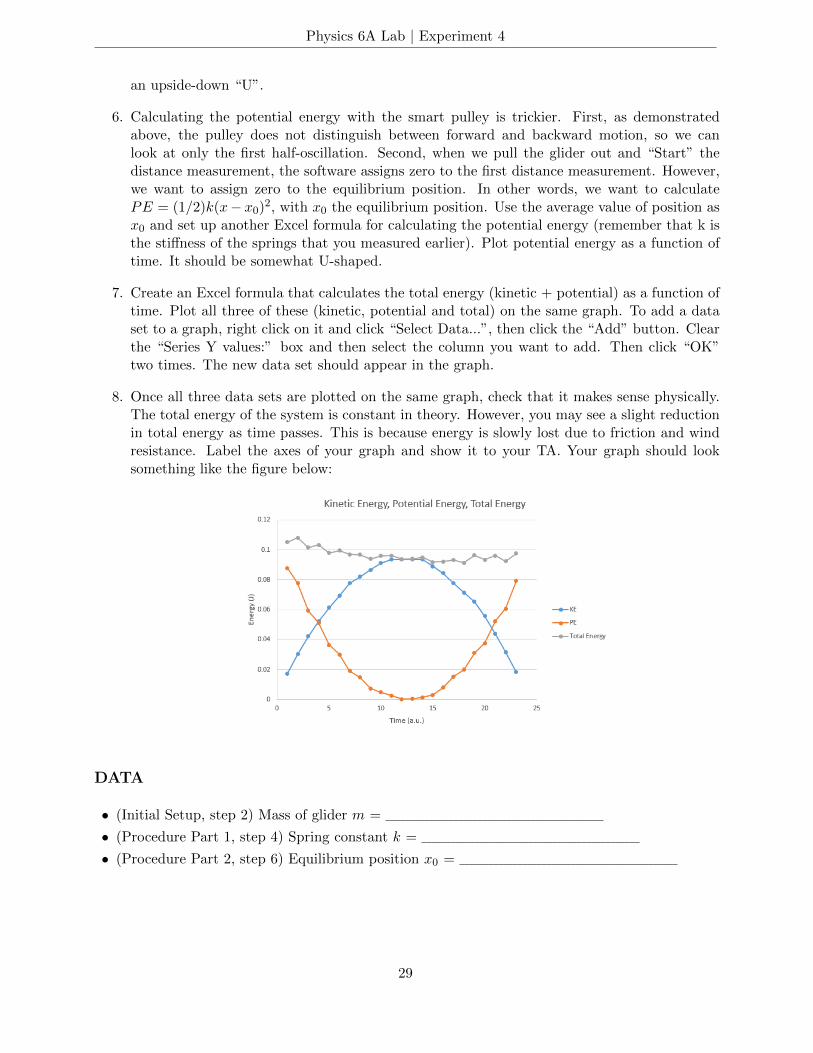
8. Once all three data sets are plotted on the same graph, check that it makes sense physically.The total energy of the system is constant in theory. However, you may see a slight reductionin total energy as time passes. This is because energy is slowly lost due to friction and windresistance. Label the axes of your graph and show it to your TA. Your graph should looksomething like the figure below:
DATA
• (Initial Setup, step 2) Mass of glider m =
• (Procedure Part 1, step 4) Spring constant k =
• (Procedure Part 2, step 6) Equilibrium position x0 =
29
Physics 6A Lab | Experiment 4
ADDITIONAL CREDIT (3 mills)
The glider-spring system is a simple harmonic oscillator. You will study the physics of such systemslater in the course. A crucial feature of such systems is that their motion is cyclic, repeating itselfwith a certain frequency. Your task is to determine this frequency.
An object’s motion is cyclic only if the motion repeats itself after a given time interval. The timethe motion takes to repeat itself is called the period of the motion. The frequency f of the cycle isthen defined as the number of cycles per unit time, and is related to the period by
fexperimental = 1/T
First devise a method and obtain the frequency of oscillation from your Capstone measurements(or make new measurements). Next use your values of k and m to check your result against thefollowing formula for the frequency of oscillation:
ftheoretical =1
2π
√k/m.
Report the results with experimental error.
30
Physics 6A Lab | Experiment 5
Momentum and Impulse
APPARATUS
Shown in the picture below:
• Air track
• Glider with bumper and flag
• Photogate
• Force sensor
Not shown in the picture above:
• Computer and Pasco interface
• Vernier calipers or meter stick to measure glider flag
• Scale and weight set
THEORY
Newton’s Second Law tells us that the net force acting on an object is equal to the object’s massmultiplied by its acceleration: Fnet = ma. Using a = dv/dt, where v is the object’s velocity, wecan rewrite this law as
Fnet = mdv/dt. (1)
Newton himself believed that this relation should also account for the possibility that the mass isvarying:
Fnet = d(mv)/dt. (2)
Examples of varying masses include rain falling into a rolling open box car and a rocket expellinggases. The above equation can be rewritten as
Fnet = dp/dt, (3)
where p = mv is the momentum of the object. Eq. 3 is the most general definition of force: thechange of momentum with time. If we write it as a differential equation,
dp = Fnetdt, (4)
31
Physics 6A Lab | Experiment 5
and integrate with respect to time, then Eq. 3 becomes
∆p = p2 − p1 =
∫Fnet dt. (5)
The right side of Eq. 5 is known as the impulse, and the left side is the change in momentum. Thenotion of impulse is often associated with a force that acts for a short period of time. Examplesof such forces include a bat hitting a ball and the impact between two objects moving at relativelyhigh speeds.
In this experiment, you will verify Eq. 5 by allowing a glider on an air track to pass through aphotogate and strike a force sensor. The sensor allows you to measure the force on the glider asa function of time. This time interval is relatively short, so the impulse approximation is valid.The velocity of the glider is measured when it crosses the photogate, just before and just afterthe collision. These two velocity measurements, along with knowledge of the glider’s mass, allowyou to calculate the change in momentum (i.e., the left side of Eq. 5). The sensor generates aforce-versus-time curve on the computer, which can be integrated to obtain the impulse (i.e., theright side of Eq. 5). The glider has a foam bumper, so its collision with the force sensor is inelastic.In other words, kinetic energy is not conserved during the collision, but the change in momentumis still equal to the impulse.
PROCEDURE
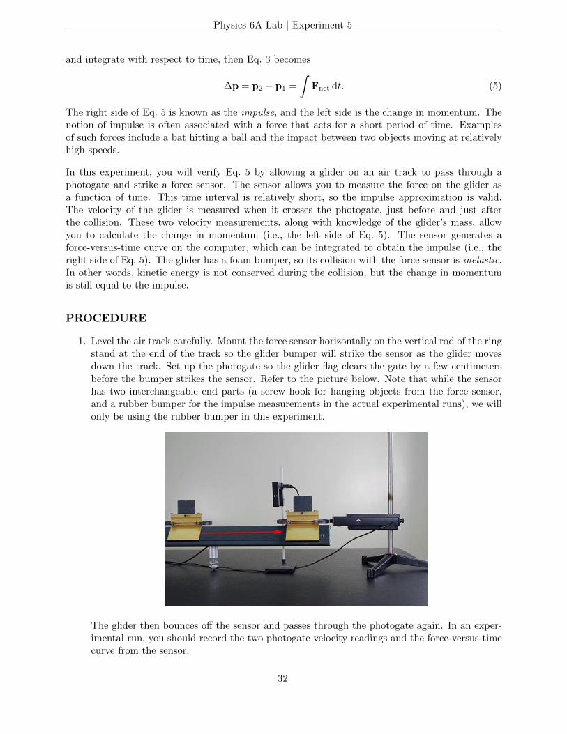
1. Level the air track carefully. Mount the force sensor horizontally on the vertical rod of the ringstand at the end of the track so the glider bumper will strike the sensor as the glider movesdown the track. Set up the photogate so the glider flag clears the gate by a few centimetersbefore the bumper strikes the sensor. Refer to the picture below. Note that while the sensorhas two interchangeable end parts (a screw hook for hanging objects from the force sensor,and a rubber bumper for the impulse measurements in the actual experimental runs), we willonly be using the rubber bumper in this experiment.
The glider then bounces off the sensor and passes through the photogate again. In an exper-imental run, you should record the two photogate velocity readings and the force-versus-timecurve from the sensor.
32
Physics 6A Lab | Experiment 5
2. Weigh the glider, and record its mass (in kilograms) in the “Data” section.
3. Open Capstone and choose “Table & Graph”. Under “Hardware Setup”, click on Channel 1and choose “Photogate”. Then click on Channel A and choose “Force Sensor”.
4. We want to set up the photogate to measure the velocity of the glider.
a. Click on “Timer Setup” and then click “Next” twice.
b. Select “One Photogate (Single Flag)”. Make sure “Speed” is selected and click next.
c. Make sure the flag width is entered in the white box (0.05 m). Then click “Next” andthen “Finish”.
5. Click on “Select Measurement” in one of your table columns and select “Speed (m/s)”. Clickon the y-axis of the graph and choose “Force (N)”.
6. At the bottom of the screen, set the sampling rate to 2000 Hz. Note that the computer willthen take a force reading every 1/2000, or 0.0005, second.
7. Turn on the air track, and push the “Tare” button on the side of the force sensor to zeroits readings. Click “Record” and send the glider down the track so it passes through thephotogate, strikes and bounces off the force sensor, and crosses the gate again. Click “Stop”.Your table should show two velocity readings at the top. The second velocity value is smallersince the collision is inelastic.
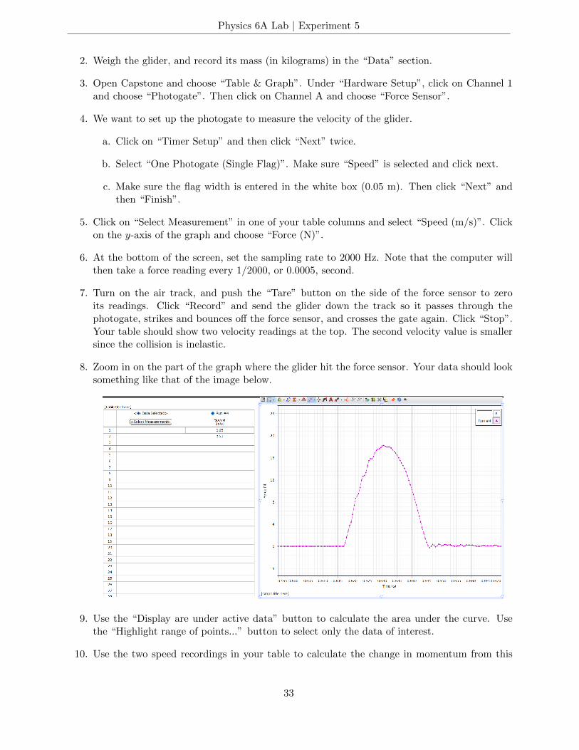
8. Zoom in on the part of the graph where the glider hit the force sensor. Your data should looksomething like that of the image below.
9. Use the “Display are under active data” button to calculate the area under the curve. Usethe “Highlight range of points...” button to select only the data of interest.
10. Use the two speed recordings in your table to calculate the change in momentum from this
33
Physics 6A Lab | Experiment 5
collision. When you calculate the change in momentum from mv1 to mv2, should you add orsubtract these two numbers? Pay attention to the direction the glider is moving and rememberthat the photogate measures speed, not velocity.
11. Have each lab partner make three measurements with different glider speeds to check therelation ∆p =
∫Fnetdt.
12. In the “Data” section, record the three values of change in momentum and impulse, as wellas the percentage difference between each set of values.
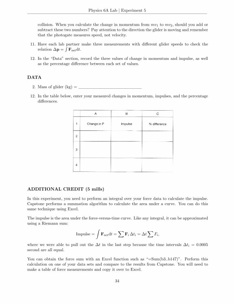
DATA
2. Mass of glider (kg) =
12. In the table below, enter your measured changes in momentum, impulses, and the percentagedifferences.
ADDITIONAL CREDIT (5 mills)
In this experiment, you need to perform an integral over your force data to calculate the impulse.Capstone performs a summation algorithm to calculate the area under a curve. You can do thissame technique using Excel.
The impulse is the area under the force-versus-time curve. Like any integral, it can be approximatedusing a Riemann sum:
Impulse =
∫Fnetdt =
∑Fi ∆ti = ∆t
∑Fi,
where we were able to pull out the ∆t in the last step because the time intervals ∆ti = 0.0005second are all equal.
You can obtain the force sum with an Excel function such as “=Sum(b3..b147)”. Perform thiscalculation on one of your data sets and compare to the results from Capstone. You will need tomake a table of force measurements and copy it over to Excel.
34

Physics 6A Lab | Experiment 5
Finally, use this force sum to calculate the impulse. As in the main part of the lab, compate thisvalue to the glider’s change in momentum and calculate the percent error.
35
Physics 6A Lab | Experiment 6
Biceps Muscle Model
Introduction
This lab will begin with some warm-up exercises to familiarize yourself with the theory, as well asthe experimental setup. Then you’ll move on to the experiment itself.
Rather than giving you explicit steps to follow at every stage, at times we’ll provide you with aproblem to investigate and some hints on how to proceed. It will be something of a challenge tofigure out how exactly to accomplish each step, but this will be much more like doing science in thereal world. We hope you enjoy the process!
Learning outcomes
By the end of this lab, you will be able to:
i. Describe how torque depends on applied force and distance of force from pivot point.
ii. Understand that angle at which a force is applied affects the applied torque.
iii. Use concepts of torque to understand aspects of the human arm.
iv. Relate the biceps muscle force to weight lifted by the hand.
v. Extrapolate a linear model from experimental data
vi. Use experimental results and critical thinking to make predictions about future results
36
Physics 6A Lab | Experiment 6
Warm up exercises
Warm up I: Torque
Before you start the main portion of the lab, here are some warm up questions to introduce you tothe key concept of torque.
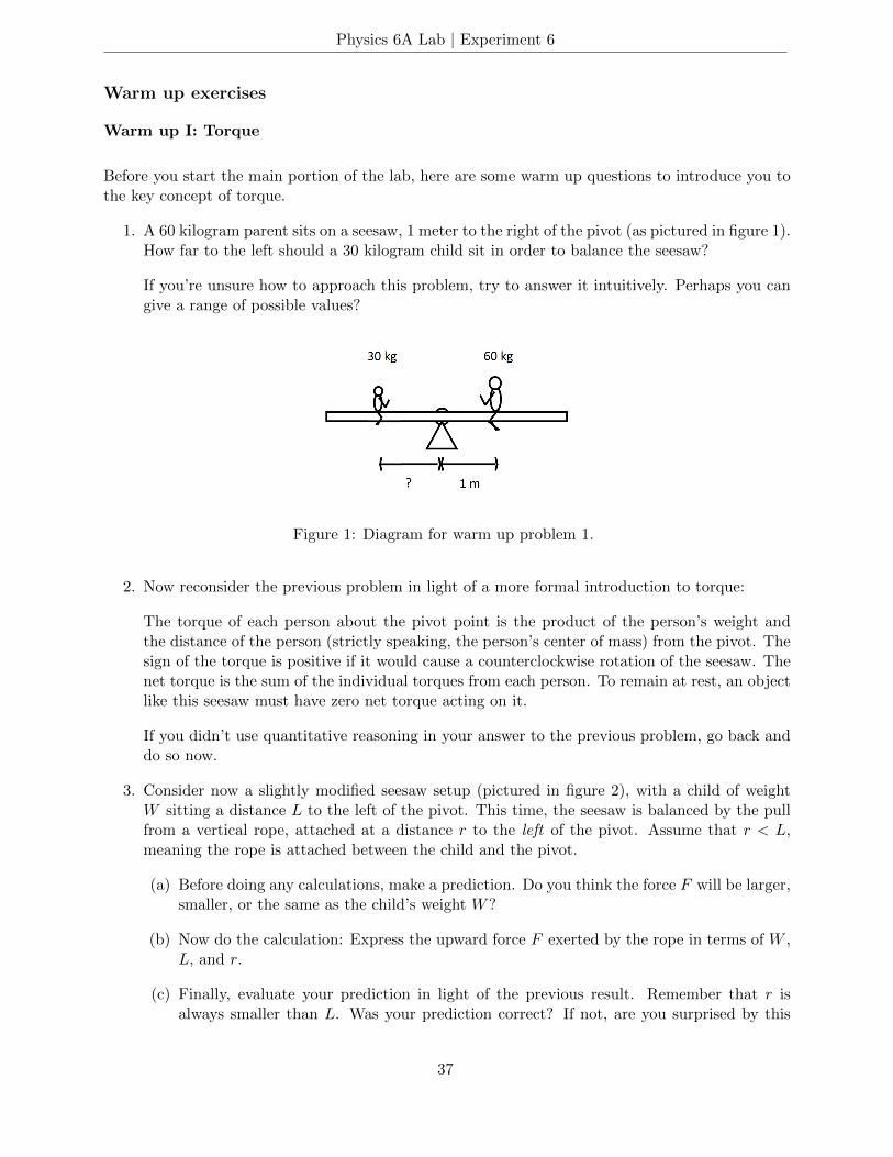
1. A 60 kilogram parent sits on a seesaw, 1 meter to the right of the pivot (as pictured in figure 1).How far to the left should a 30 kilogram child sit in order to balance the seesaw?
If you’re unsure how to approach this problem, try to answer it intuitively. Perhaps you cangive a range of possible values?
Figure 1: Diagram for warm up problem 1.
2. Now reconsider the previous problem in light of a more formal introduction to torque:
The torque of each person about the pivot point is the product of the person’s weight andthe distance of the person (strictly speaking, the person’s center of mass) from the pivot. Thesign of the torque is positive if it would cause a counterclockwise rotation of the seesaw. Thenet torque is the sum of the individual torques from each person. To remain at rest, an objectlike this seesaw must have zero net torque acting on it.
If you didn’t use quantitative reasoning in your answer to the previous problem, go back anddo so now.
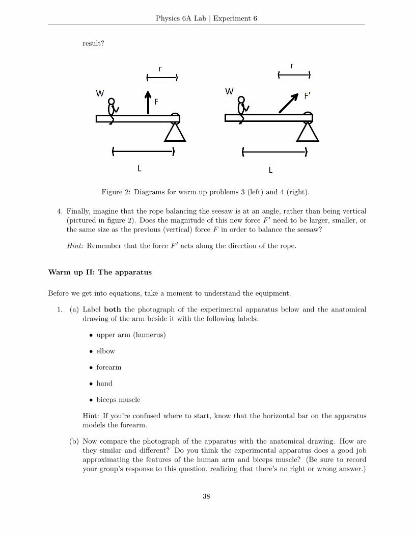
3. Consider now a slightly modified seesaw setup (pictured in figure 2), with a child of weightW sitting a distance L to the left of the pivot. This time, the seesaw is balanced by the pullfrom a vertical rope, attached at a distance r to the left of the pivot. Assume that r < L,meaning the rope is attached between the child and the pivot.
(a) Before doing any calculations, make a prediction. Do you think the force F will be larger,smaller, or the same as the child’s weight W?
(b) Now do the calculation: Express the upward force F exerted by the rope in terms of W ,L, and r.
(c) Finally, evaluate your prediction in light of the previous result. Remember that r isalways smaller than L. Was your prediction correct? If not, are you surprised by this
37
Physics 6A Lab | Experiment 6
result?
Figure 2: Diagrams for warm up problems 3 (left) and 4 (right).
4. Finally, imagine that the rope balancing the seesaw is at an angle, rather than being vertical(pictured in figure 2). Does the magnitude of this new force F ′ need to be larger, smaller, orthe same size as the previous (vertical) force F in order to balance the seesaw?
Hint: Remember that the force F ′ acts along the direction of the rope.
Warm up II: The apparatus
Before we get into equations, take a moment to understand the equipment.
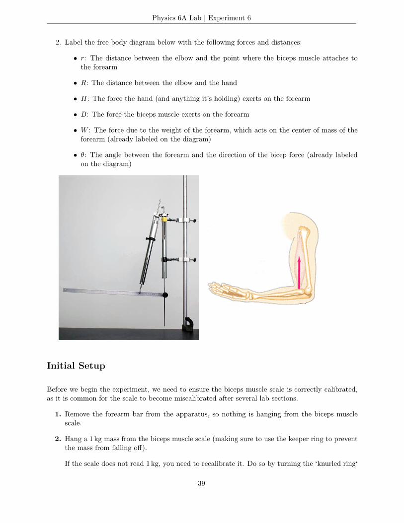
1. (a) Label both the photograph of the experimental apparatus below and the anatomicaldrawing of the arm beside it with the following labels:
• upper arm (humerus)
• elbow
• forearm
• hand
• biceps muscle
Hint: If you’re confused where to start, know that the horizontal bar on the apparatusmodels the forearm.
(b) Now compare the photograph of the apparatus with the anatomical drawing. How arethey similar and different? Do you think the experimental apparatus does a good jobapproximating the features of the human arm and biceps muscle? (Be sure to recordyour group’s response to this question, realizing that there’s no right or wrong answer.)
38
Physics 6A Lab | Experiment 6
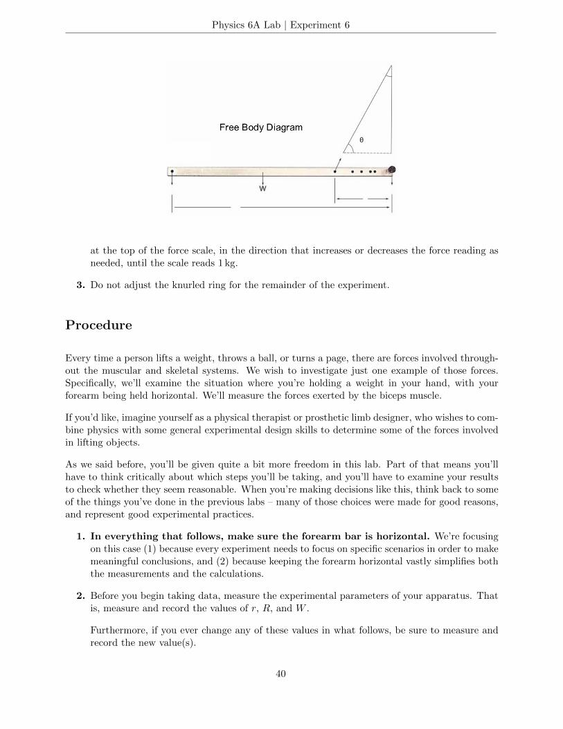
2. Label the free body diagram below with the following forces and distances:
• r: The distance between the elbow and the point where the biceps muscle attaches tothe forearm
• R: The distance between the elbow and the hand
• H: The force the hand (and anything it’s holding) exerts on the forearm
• B: The force the biceps muscle exerts on the forearm
• W : The force due to the weight of the forearm, which acts on the center of mass of theforearm (already labeled on the diagram)
• θ: The angle between the forearm and the direction of the bicep force (already labeledon the diagram)
Initial Setup
Before we begin the experiment, we need to ensure the biceps muscle scale is correctly calibrated,as it is common for the scale to become miscalibrated after several lab sections.
1. Remove the forearm bar from the apparatus, so nothing is hanging from the biceps musclescale.
2. Hang a 1 kg mass from the biceps muscle scale (making sure to use the keeper ring to preventthe mass from falling off).
If the scale does not read 1 kg, you need to recalibrate it. Do so by turning the ‘knurled ring‘
39
Physics 6A Lab | Experiment 6
at the top of the force scale, in the direction that increases or decreases the force reading asneeded, until the scale reads 1 kg.
3. Do not adjust the knurled ring for the remainder of the experiment.
Procedure
Every time a person lifts a weight, throws a ball, or turns a page, there are forces involved through-out the muscular and skeletal systems. We wish to investigate just one example of those forces.Specifically, we’ll examine the situation where you’re holding a weight in your hand, with yourforearm being held horizontal. We’ll measure the forces exerted by the biceps muscle.
If you’d like, imagine yourself as a physical therapist or prosthetic limb designer, who wishes to com-bine physics with some general experimental design skills to determine some of the forces involvedin lifting objects.
As we said before, you’ll be given quite a bit more freedom in this lab. Part of that means you’llhave to think critically about which steps you’ll be taking, and you’ll have to examine your resultsto check whether they seem reasonable. When you’re making decisions like this, think back to someof the things you’ve done in the previous labs – many of those choices were made for good reasons,and represent good experimental practices.
1. In everything that follows, make sure the forearm bar is horizontal. We’re focusingon this case (1) because every experiment needs to focus on specific scenarios in order to makemeaningful conclusions, and (2) because keeping the forearm horizontal vastly simplifies boththe measurements and the calculations.
2. Before you begin taking data, measure the experimental parameters of your apparatus. Thatis, measure and record the values of r, R, and W .
Furthermore, if you ever change any of these values in what follows, be sure to measure andrecord the new value(s).
40
Physics 6A Lab | Experiment 6
Note that for the first several steps, you’ll be keeping r fixed. It’s up to you to choose whicheverinitial value for r you’d like, but we recommend starting with a fairly large r.
3. Start by measuring the biceps force B for some fixed weight H being held in the hand. Makesure to record this value (with units). Note that the force gauges are labelled with units ofmass (kilograms) rather than units of force (Newtons). You need to multiply the mass readingsby g = 9.8 m/s2 to convert the mass values to their corresponding weight values. Note thatyou may wish to first just record the mass values, and convert to weight using Excel.
B =(
Biceps gauge reading (in kilograms))× g
After doing this, B and H should both be recorded in units of force.
Note: H corresponds to the weight held by the hand – that is, the weight hanging off theforearm bar. It does not include the weight of the forearm, which is separately accounted forin W . (W , in turn, does not include the weight held by the hand.)
4. Now devise and carry out a procedure for measuring (and recording) the force B for differentweights H. Make sure to explicitly write out the steps of the procedure. If you find you needto modify the procedure as you carry it out, that’s okay – but be sure to change the writtenversion to correctly reflect the steps you really carried out.
5. After taking several measurements (you can choose a number which seems reasonable), useyour data to extrapolate a relationship between the biceps force B and the weight H in thehand: First, argue that your data shows a linear relationship between B and H. Then, writean explicit formula for B as a function of H. Hint: In case this terminology is a bit unfamiliar,
it might help to know that y(t) =(
10 m)−(
4.9 m/s2)t2 is an example of an explicit formula
for y as a function of t (for a certain physical situation). Make sure you specify the units ofall quantities involved. Hint: You’ve performed similar steps in previous labs. Think back toany time you graphed your data and fit a trendline to the graph.
6. Choose a new value for H – one that you haven’t measured yet, but that you are able tomeasure. Before you measure B, use your model to predict the biceps force B for this newvalue of H.
7. Now use the apparatus to measure B for this value ofH. How does it compare to the predictionfrom your model? (Calculate the percent deviation.) If the two values don’t exactly agree,do you think this is okay? Do you think it tells us our model is wrong? Why or why not?
8. Is your formula for B as a function of H consistent with the concepts of torque explored inthe warmup problems? Why or why not?
Varying model parameters
Now that you’ve gained a bit of familiarity with the apparatus by taking some measurements, let’stake a step back and think a bit more about what’s going on.
9. Using a combination of your intuition for how your own arm works, and the knowledge oftorque you developed in the warm up exercises, predict how the biceps force change when we
41
Physics 6A Lab | Experiment 6
increase each of the following parameters.
Fill in your own copy of the charts below, answering with “increases”, “decreases”, “staysconstant”, or “something else”. (If you choose something else, explain why you chose that.)
Parameter change Effect on B
↑ R↑W↑ r
10. The way our apparatus is set up, the easiest of the above parameters to vary experimentallyis r. Devise and carry out an experiment to determine the effect that increasing r has onthe biceps force B. Make sure to record the data that leads you to this conclusion. Do yourresults agree with your prediction in part 9?
Comparing results to theoretical predictions
In a previous step above, you experimentally determined a formula for the biceps force B as afunction of the weight H in the hand. Now we’ll compare this model to the one the theory predicts.
It turns out that we can analyze the torques acting on the forearm to determine a formula for B vsH. You actually have all the tools needed to do this from the warm up exercises at the beginningof this lab, and we encourage you to give it a try! But in the interest of time, we’ll just provide youwith the formula, which is as follows:
B =
(H +
W
2
)R
r sin θ
11. Now that we have this theoretical model, we can use it to predict what the slope and verticalintercept of your graph of B vs H should be. First, use the theoretical model to predict theslope and vertical intercept of your graph in terms of symbols (i.e., variables) only. Next,plug in the actual parameter values that correspond to your experimental apparatus to geta numerical value for these theoretical coefficients (with units!). How does this predictioncompare with your actual slope and vertical intercept?
Note: If you need to find the angle θ, you can do so by measuring two sides of the righttriangle formed by the upper arm, the forearm, and the biceps muscle. You can then use theappropriate inverse trig function to find θ.
12. Using the formula above for B as a function of H, revist your predictions from part 9. Thatis, argue whether the formula given to you above agrees or disagrees with the predictions youmade before.
Wrapping up
13. Note: This problem involves a bit of reading, but it should help you understand the importanceof a key concept, which will help you on your homework and exams.
42
Physics 6A Lab | Experiment 6
Imagine you and a friend wanted to predict the biceps force by directly analyzing the torquesinvolve in the apparatus. You and your friend determine that the experimental parametersfor your apparatus are R = 50 cm, r = 25 cm, W = 2.5 N, H = 2.5 N. Your friend attempts touse the theoretical model to predict the value of the biceps force. He claims that the torqueexerted by the biceps must be equal and opposite to the torque exerted by the weight in thehand plus the weight of the arm itself, which is equal to HR+WR/2, in the counter clockwisedirection. Furthermore, your friend claims that the torque due to the biceps is Br, in theclockwise direction. Since the torques must be equal and opposite, we have Br = HR+WR/2.
You read the biceps gauge and find it reads about 0.85 kilograms. Solve the equation abovefor B, and plug in the values of the experimental parameters given above. Does the resultingvalue for B agrees with the measured biceps force?
If your prediction is not consistent with the experimental result, go back and figure out whatwas wrong with your friend’s argument above.
Was there a key torque concept your friend forgot to take into account?
43
Physics 6A Lab | Experiment 7
Rotation and Gyroscopic Precession
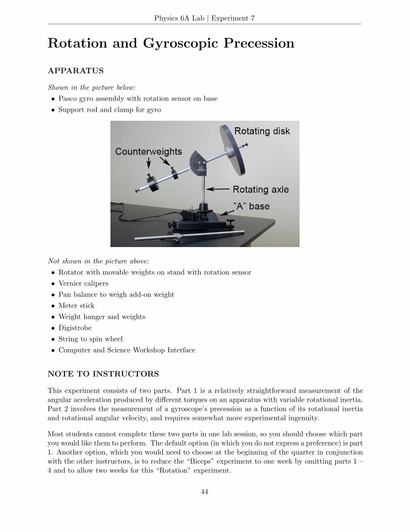
APPARATUS
Shown in the picture below:
• Pasco gyro assembly with rotation sensor on base
• Support rod and clamp for gyro
Not shown in the picture above:
• Rotator with movable weights on stand with rotation sensor
• Vernier calipers
• Pan balance to weigh add-on weight
• Meter stick
• Weight hanger and weights
• Digistrobe
• String to spin wheel
• Computer and Science Workshop Interface
NOTE TO INSTRUCTORS
This experiment consists of two parts. Part 1 is a relatively straightforward measurement of theangular acceleration produced by different torques on an apparatus with variable rotational inertia.Part 2 involves the measurement of a gyroscope’s precession as a function of its rotational inertiaand rotational angular velocity, and requires somewhat more experimental ingenuity.
Most students cannot complete these two parts in one lab session, so you should choose which partyou would like them to perform. The default option (in which you do not express a preference) is part1. Another option, which you would need to choose at the beginning of the quarter in conjunctionwith the other instructors, is to reduce the “Biceps” experiment to one week by omitting parts 1 –4 and to allow two weeks for this “Rotation” experiment.
44
Physics 6A Lab | Experiment 7
TORQUE AND ROTATIONAL INERTIA
We are all aware that a massive wheel has rotational inertia. In other words, it is hard to startthe wheel rotating; and, once moving, the wheel tends to continue rotating and is hard to stop.These effects are independent of friction; it is hard to start a wheel rotating even if its bearings arenearly frictionless. Rotational inertia is a measure of this resistance to rotational acceleration, justas inertia is a measure of resistance to linear acceleration.
Automobile piston engines use a flywheel for this very purpose. The gasoline explosions in thepiston chambers deliver jerk-like forces to the rotating crankshaft, but the large rotational inertiaof the flywheel on the crankshaft smooths out the otherwise jerky rotational motion.
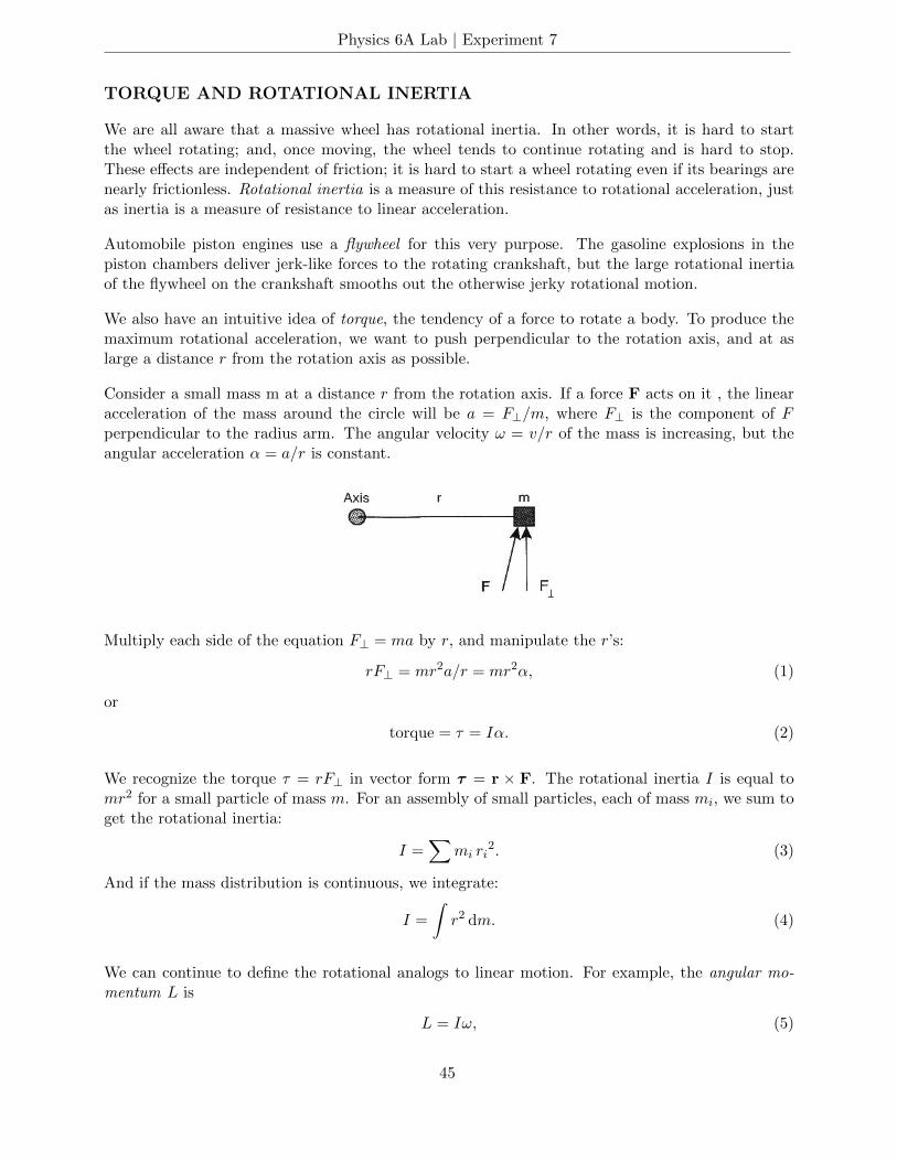
We also have an intuitive idea of torque, the tendency of a force to rotate a body. To produce themaximum rotational acceleration, we want to push perpendicular to the rotation axis, and at aslarge a distance r from the rotation axis as possible.
Consider a small mass m at a distance r from the rotation axis. If a force F acts on it , the linearacceleration of the mass around the circle will be a = F⊥/m, where F⊥ is the component of Fperpendicular to the radius arm. The angular velocity ω = v/r of the mass is increasing, but theangular acceleration α = a/r is constant.
Multiply each side of the equation F⊥ = ma by r, and manipulate the r’s:
rF⊥ = mr2a/r = mr2α, (1)
or
torque = τ = Iα. (2)
We recognize the torque τ = rF⊥ in vector form τ = r × F. The rotational inertia I is equal tomr2 for a small particle of mass m. For an assembly of small particles, each of mass mi, we sum toget the rotational inertia:
I =∑
mi ri2. (3)
And if the mass distribution is continuous, we integrate:
I =
∫r2 dm. (4)
We can continue to define the rotational analogs to linear motion. For example, the angular mo-mentum L is
L = Iω, (5)
45
Physics 6A Lab | Experiment 7
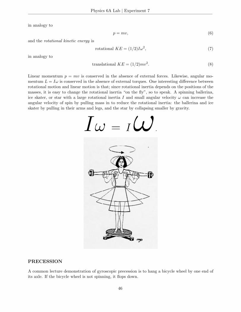
in analogy to
p = mv, (6)
and the rotational kinetic energy is
rotational KE = (1/2)Iω2, (7)
in analogy to
translational KE = (1/2)mv2. (8)
Linear momentum p = mv is conserved in the absence of external forces. Likewise, angular mo-mentum L = Iω is conserved in the absence of external torques. One interesting difference betweenrotational motion and linear motion is that; since rotational inertia depends on the positions of themasses, it is easy to change the rotational inertia “on the fly”, so to speak. A spinning ballerina,ice skater, or star with a large rotational inertia I and small angular velocity ω can increase theangular velocity of spin by pulling mass in to reduce the rotational inertia: the ballerina and iceskater by pulling in their arms and legs, and the star by collapsing smaller by gravity.
PRECESSION
A common lecture demonstration of gyroscopic precession is to hang a bicycle wheel by one end ofits axle. If the bicycle wheel is not spinning, it flops down.
46
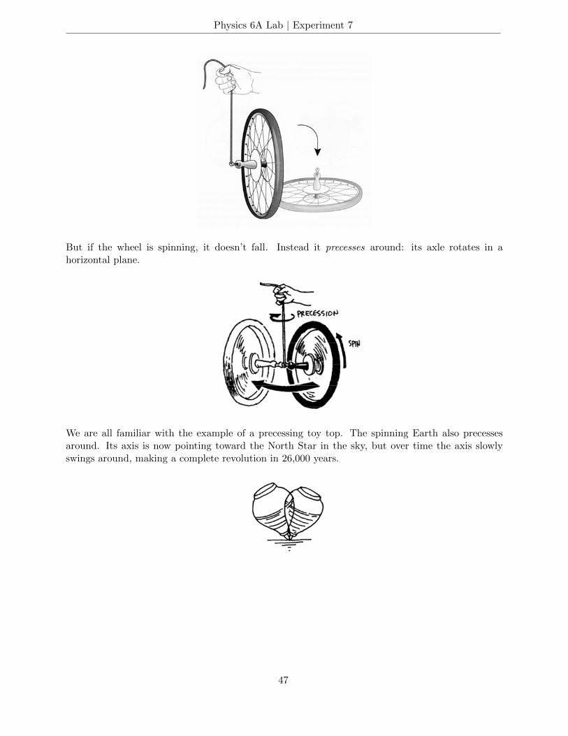
Physics 6A Lab | Experiment 7
But if the wheel is spinning, it doesn’t fall. Instead it precesses around: its axle rotates in ahorizontal plane.
We are all familiar with the example of a precessing toy top. The spinning Earth also precessesaround. Its axis is now pointing toward the North Star in the sky, but over time the axis slowlyswings around, making a complete revolution in 26,000 years.
47
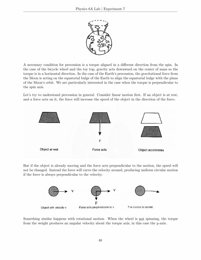
Physics 6A Lab | Experiment 7
A necessary condition for precession is a torque aligned in a different direction from the spin. Inthe case of the bicycle wheel and the toy top, gravity acts downward on the center of mass so thetorque is in a horizontal direction. In the case of the Earth’s precession, the gravitational force fromthe Moon is acting on the equatorial bulge of the Earth to align the equatorial bulge with the planeof the Moon’s orbit. We are particularly interested in the case when the torque is perpendicular tothe spin axis.
Let’s try to understand precession in general. Consider linear motion first. If an object is at rest,and a force acts on it, the force will increase the speed of the object in the direction of the force.
But if the object is already moving and the force acts perpendicular to the motion, the speed willnot be changed. Instead the force will curve the velocity around, producing uniform circular motionif the force is always perpendicular to the velocity.
Something similar happens with rotational motion. When the wheel is not spinning, the torquefrom the weight produces an angular velocity about the torque axis, in this case the y-axis.
48
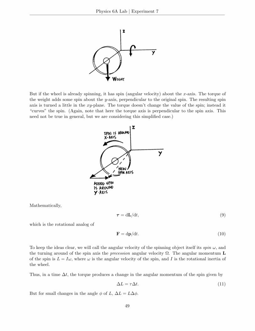
Physics 6A Lab | Experiment 7
But if the wheel is already spinning, it has spin (angular velocity) about the x-axis. The torque ofthe weight adds some spin about the y-axis, perpendicular to the original spin. The resulting spinaxis is turned a little in the xy-plane. The torque doesn’t change the value of the spin; instead it“curves” the spin. (Again, note that here the torque axis is perpendicular to the spin axis. Thisneed not be true in general, but we are considering this simplified case.)
Mathematically,
τ = dL/dt, (9)
which is the rotational analog of
F = dp/dt. (10)
To keep the ideas clear, we will call the angular velocity of the spinning object itself its spin ω, andthe turning around of the spin axis the precession angular velocity Ω. The angular momentum Lof the spin is L = Iω, where ω is the angular velocity of the spin, and I is the rotational inertia ofthe wheel.
Thus, in a time ∆t, the torque produces a change in the angular momentum of the spin given by
∆L = τ∆t. (11)
But for small changes in the angle φ of L, ∆L = L∆φ.
49
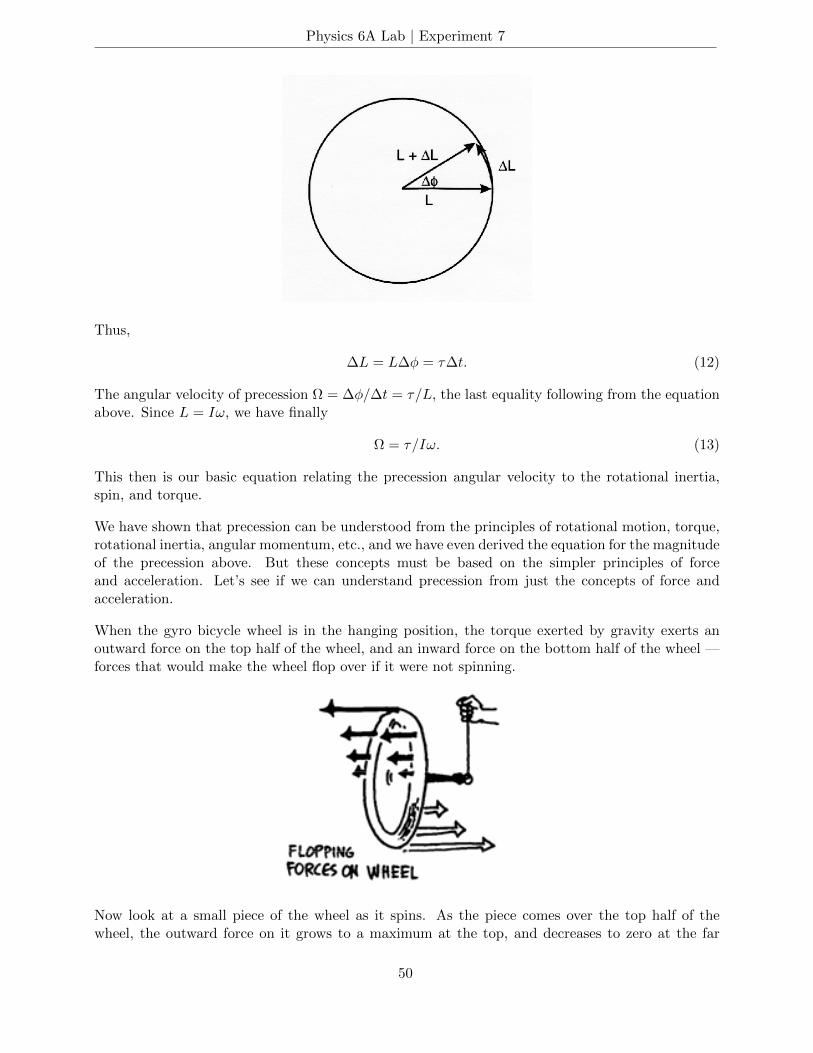
Physics 6A Lab | Experiment 7
Thus,
∆L = L∆φ = τ∆t. (12)
The angular velocity of precession Ω = ∆φ/∆t = τ/L, the last equality following from the equationabove. Since L = Iω, we have finally
Ω = τ/Iω. (13)
This then is our basic equation relating the precession angular velocity to the rotational inertia,spin, and torque.
We have shown that precession can be understood from the principles of rotational motion, torque,rotational inertia, angular momentum, etc., and we have even derived the equation for the magnitudeof the precession above. But these concepts must be based on the simpler principles of forceand acceleration. Let’s see if we can understand precession from just the concepts of force andacceleration.
When the gyro bicycle wheel is in the hanging position, the torque exerted by gravity exerts anoutward force on the top half of the wheel, and an inward force on the bottom half of the wheel —forces that would make the wheel flop over if it were not spinning.
Now look at a small piece of the wheel as it spins. As the piece comes over the top half of thewheel, the outward force on it grows to a maximum at the top, and decreases to zero at the far
50
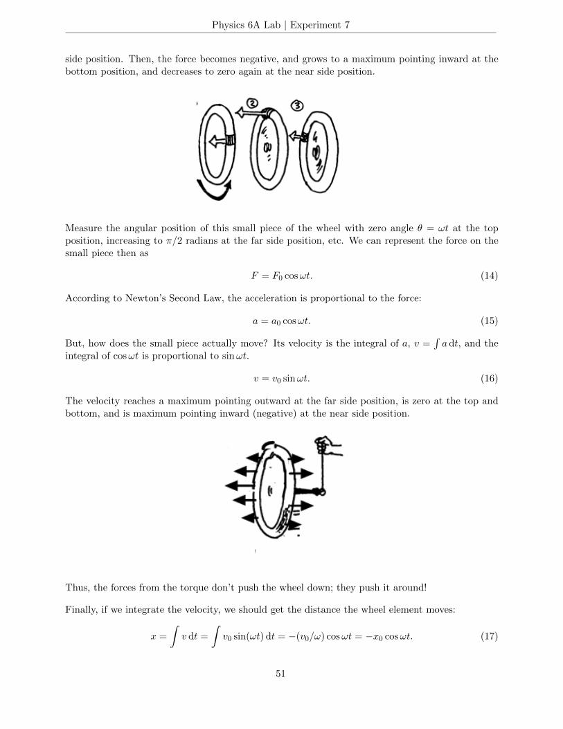
Physics 6A Lab | Experiment 7
side position. Then, the force becomes negative, and grows to a maximum pointing inward at thebottom position, and decreases to zero again at the near side position.
Measure the angular position of this small piece of the wheel with zero angle θ = ωt at the topposition, increasing to π/2 radians at the far side position, etc. We can represent the force on thesmall piece then as
F = F0 cosωt. (14)
According to Newton’s Second Law, the acceleration is proportional to the force:
a = a0 cosωt. (15)
But, how does the small piece actually move? Its velocity is the integral of a, v =∫a dt, and the
integral of cosωt is proportional to sinωt.
v = v0 sinωt. (16)
The velocity reaches a maximum pointing outward at the far side position, is zero at the top andbottom, and is maximum pointing inward (negative) at the near side position.
Thus, the forces from the torque don’t push the wheel down; they push it around!
Finally, if we integrate the velocity, we should get the distance the wheel element moves:
x =
∫v dt =
∫v0 sin(ωt) dt = −(v0/ω) cosωt = −x0 cosωt. (17)
51
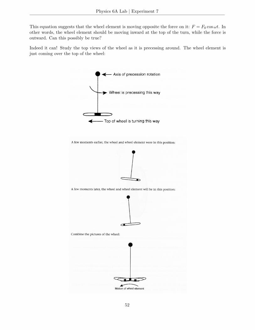
Physics 6A Lab | Experiment 7
This equation suggests that the wheel element is moving opposite the force on it: F = F0 cosωt. Inother words, the wheel element should be moving inward at the top of the turn, while the force isoutward. Can this possibly be true?
Indeed it can! Study the top views of the wheel as it is precessing around. The wheel element isjust coming over the top of the wheel:
52
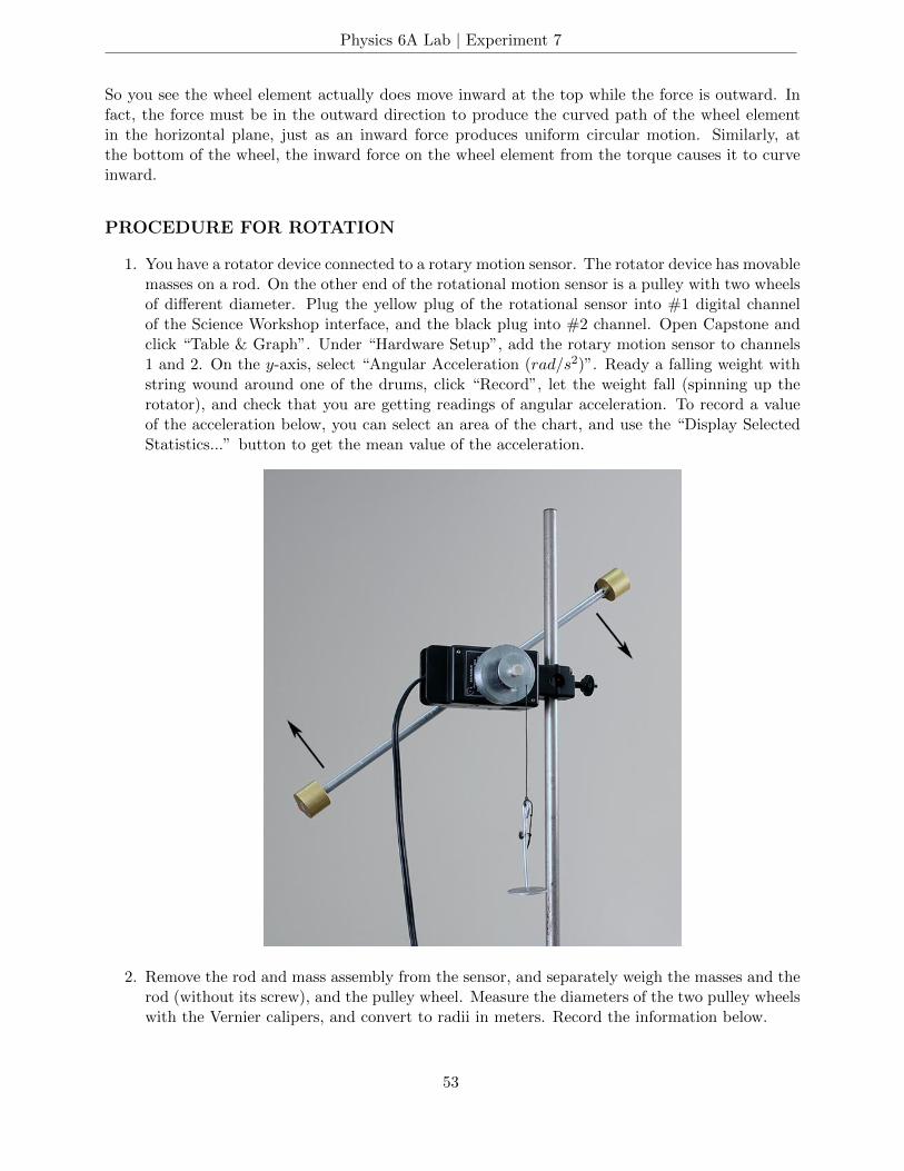
Physics 6A Lab | Experiment 7
So you see the wheel element actually does move inward at the top while the force is outward. Infact, the force must be in the outward direction to produce the curved path of the wheel elementin the horizontal plane, just as an inward force produces uniform circular motion. Similarly, atthe bottom of the wheel, the inward force on the wheel element from the torque causes it to curveinward.
PROCEDURE FOR ROTATION
1. You have a rotator device connected to a rotary motion sensor. The rotator device has movablemasses on a rod. On the other end of the rotational motion sensor is a pulley with two wheelsof different diameter. Plug the yellow plug of the rotational sensor into #1 digital channelof the Science Workshop interface, and the black plug into #2 channel. Open Capstone andclick “Table & Graph”. Under “Hardware Setup”, add the rotary motion sensor to channels1 and 2. On the y-axis, select “Angular Acceleration (rad/s2)”. Ready a falling weight withstring wound around one of the drums, click “Record”, let the weight fall (spinning up therotator), and check that you are getting readings of angular acceleration. To record a valueof the acceleration below, you can select an area of the chart, and use the “Display SelectedStatistics...” button to get the mean value of the acceleration.
2. Remove the rod and mass assembly from the sensor, and separately weigh the masses and therod (without its screw), and the pulley wheel. Measure the diameters of the two pulley wheelswith the Vernier calipers, and convert to radii in meters. Record the information below.
53
Physics 6A Lab | Experiment 7
Mass of movable weights in kilograms =
Mass of rod without screw =
Mass of pulley wheel =
Radius of small pulley in meters =
Radius of large pulley in meters =
Warning: In rotational experiments it is especially important to keep mass units (asin rotational inertia) and force units (as in torque) clearly distinguished.
3. According to the textbook, the rotational inertia of a rod of mass m and length l about anaxis perpendicular to the rod and through its center is (1/12)ml2. Calculate the rotationalinertia of the rod. Does it make any difference that the rod is hollow?
I of rod in kg ·m2 =
4. From the mass of the pulley wheel and its volume (which you can calculate from the radiiof the two parts), you can calculate its density. From this you can calculate the rotationalinertia of the pulley wheel. You may have to do some estimating.
I of pulley wheel in kg ·m2 =
5. Do a trial experimental run in which the masses on the rotator are at the ends of the rodso that the rotational inertia is large. Use 100 – 200 g on the weight hanger and wind thestring around the smaller pulley wheel. (This should be the smallest angular accelerationcase.) Notice that the angular acceleration on the graph quickly jumps up and reaches anapproximately constant value. You can select an area of this nearly constant value, and usethe statistics button to get its mean value for the “measured angular acceleration” in thetable below. Now do a trial experimental run in which the masses on the rotator are closeto the center so that the rotational inertia is small. Use 100 – 200 g on the weight hangerand wind the string around the larger pulley wheel so that the torque will spin the rotator upto high speed. (This should be the largest angular acceleration case.) On the graph, noticethat the acceleration quickly reaches a peak, and then falls off with time. Why isn’t the ofacceleration constant in this case? Where on the acceleration curve should you average thevalues of acceleration to get a good result to compare with the predicted acceleration? Howcan you adjust the apparatus or experimental parameters to get a better result for the smallrotational inertia case?
6. Using masses of 50 – 200 grams, hook the string on the pulley pin, wind the string around thepulley, and let the mass fall while you measure the rotational acceleration on the computer. Dothree experimental trials for each case, and average them to find the rotational acceleration.
54
Physics 6A Lab | Experiment 7
Do four cases: two different positions of the masses on the rod (as close to the center aspossible, and as far out as possible), and two different pulley sizes. Compute the rotationalinertia of the rod with masses (add the effects of the rods, the pulley wheel, and the masses),the torque, the predicted rotational acceleration, and the experimental error, and fill in thetable below.
When you add the rotational inertias of the rod, masses, and pulley wheel to get the rotationalinertia of the entire rotating assembly, are you leaving out anything?
PROCEDURE FOR GYROSCOPE
1. We want to check the precession, equation 13, Ω = τ/Iω. Study your gyroscope for a moment.As you rotate the arm for precession, the rotary motion sensor at the base should move freely.(If not, adjust the screws that hold the sensor.) The rotary sensor from the first part of theexperiment may still be set up on Data Studio. Unplug this rotary sensor and delete all thesensors and data. (Or quit Data Studio, and open it up new.) Plug the rotary sensor of thegyro precession into the Science Workshop interface, and drag a digits window to the rotarymotion sensor symbol, and set it to measure the rotational angular velocity Ω. (You may haveto double-click on the icon of the rotary motion sensor connected to the Science Workshop,and check the “Angular Velocity Ch 1 & 2 (ras/s)” box.)
55
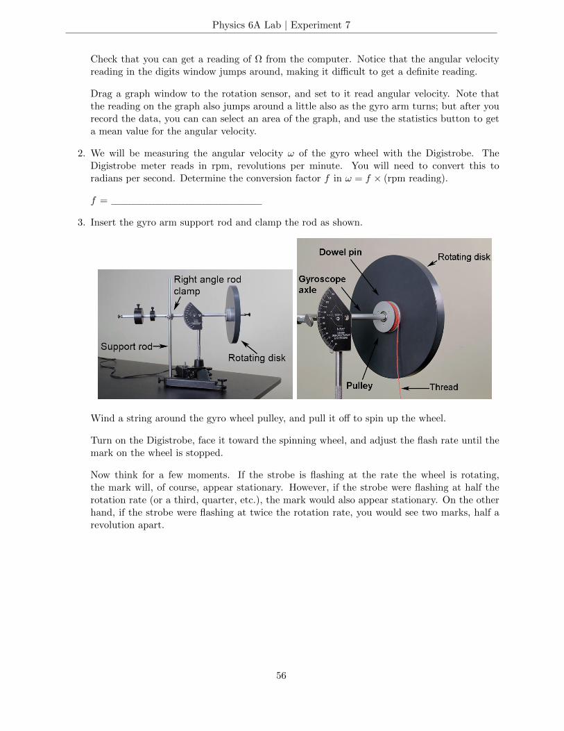
Physics 6A Lab | Experiment 7
Check that you can get a reading of Ω from the computer. Notice that the angular velocityreading in the digits window jumps around, making it difficult to get a definite reading.
Drag a graph window to the rotation sensor, and set to it read angular velocity. Note thatthe reading on the graph also jumps around a little also as the gyro arm turns; but after yourecord the data, you can can select an area of the graph, and use the statistics button to geta mean value for the angular velocity.
2. We will be measuring the angular velocity ω of the gyro wheel with the Digistrobe. TheDigistrobe meter reads in rpm, revolutions per minute. You will need to convert this toradians per second. Determine the conversion factor f in ω = f × (rpm reading).
f =
3. Insert the gyro arm support rod and clamp the rod as shown.
Wind a string around the gyro wheel pulley, and pull it off to spin up the wheel.
Turn on the Digistrobe, face it toward the spinning wheel, and adjust the flash rate until themark on the wheel is stopped.
Now think for a few moments. If the strobe is flashing at the rate the wheel is rotating,the mark will, of course, appear stationary. However, if the strobe were flashing at half therotation rate (or a third, quarter, etc.), the mark would also appear stationary. On the otherhand, if the strobe were flashing at twice the rotation rate, you would see two marks, half arevolution apart.
56
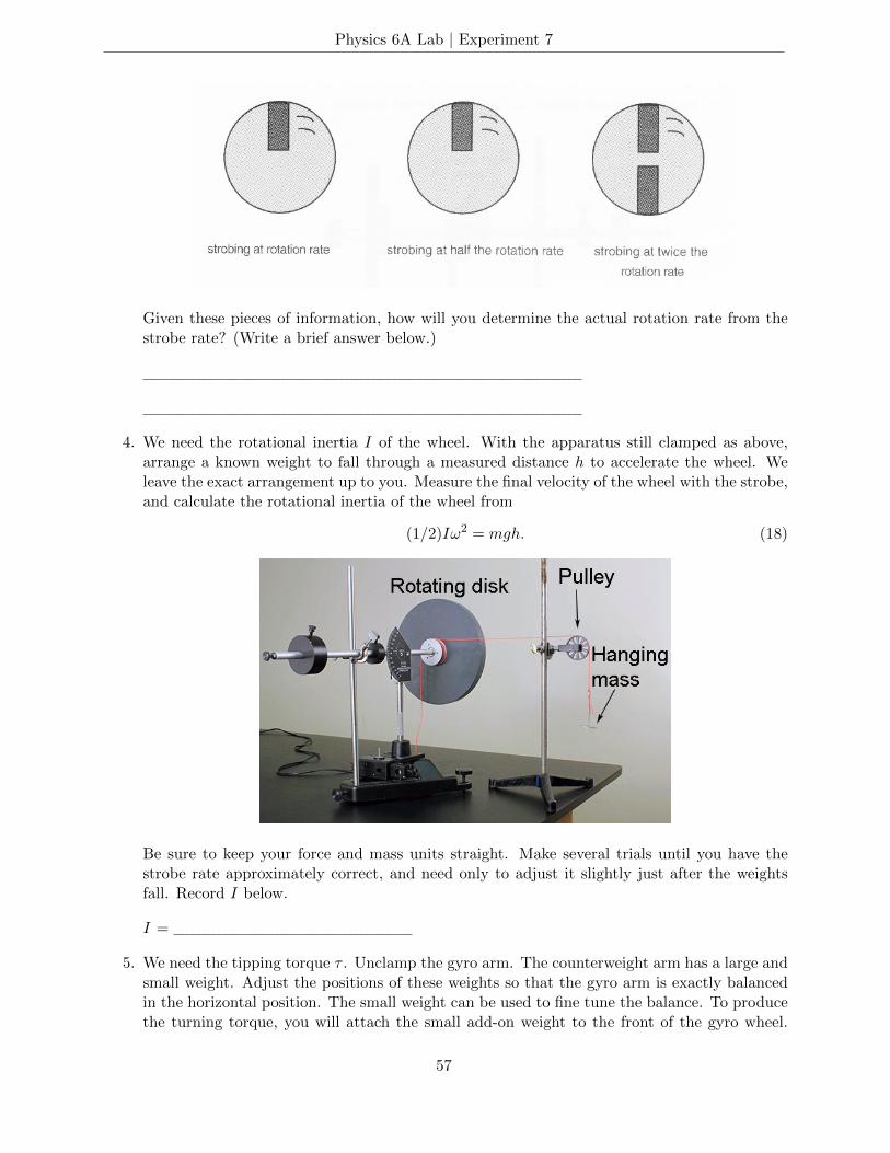
Physics 6A Lab | Experiment 7
Given these pieces of information, how will you determine the actual rotation rate from thestrobe rate? (Write a brief answer below.)
4. We need the rotational inertia I of the wheel. With the apparatus still clamped as above,arrange a known weight to fall through a measured distance h to accelerate the wheel. Weleave the exact arrangement up to you. Measure the final velocity of the wheel with the strobe,and calculate the rotational inertia of the wheel from
(1/2)Iω2 = mgh. (18)
Be sure to keep your force and mass units straight. Make several trials until you have thestrobe rate approximately correct, and need only to adjust it slightly just after the weightsfall. Record I below.
I =
5. We need the tipping torque τ . Unclamp the gyro arm. The counterweight arm has a large andsmall weight. Adjust the positions of these weights so that the gyro arm is exactly balancedin the horizontal position. The small weight can be used to fine tune the balance. To producethe turning torque, you will attach the small add-on weight to the front of the gyro wheel.
57
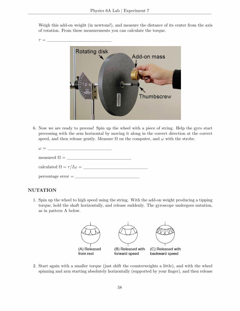
Physics 6A Lab | Experiment 7
Weigh this add-on weight (in newtons!), and measure the distance of its center from the axisof rotation. From these measurements you can calculate the torque.
τ =
6. Now we are ready to precess! Spin up the wheel with a piece of string. Help the gyro startprecessing with the arm horizontal by moving it along in the correct direction at the correctspeed, and then release gently. Measure Ω on the computer, and ω with the strobe.
ω =
measured Ω =
calculated Ω = τ/Iω =
percentage error =
NUTATION
1. Spin up the wheel to high speed using the string. With the add-on weight producing a tippingtorque, hold the shaft horizontally, and release suddenly. The gyroscope undergoes nutation,as in pattern A below.
2. Start again with a smaller torque (just shift the counterweights a little), and with the wheelspinning and arm starting absolutely horizontally (supported by your finger), and then release
58
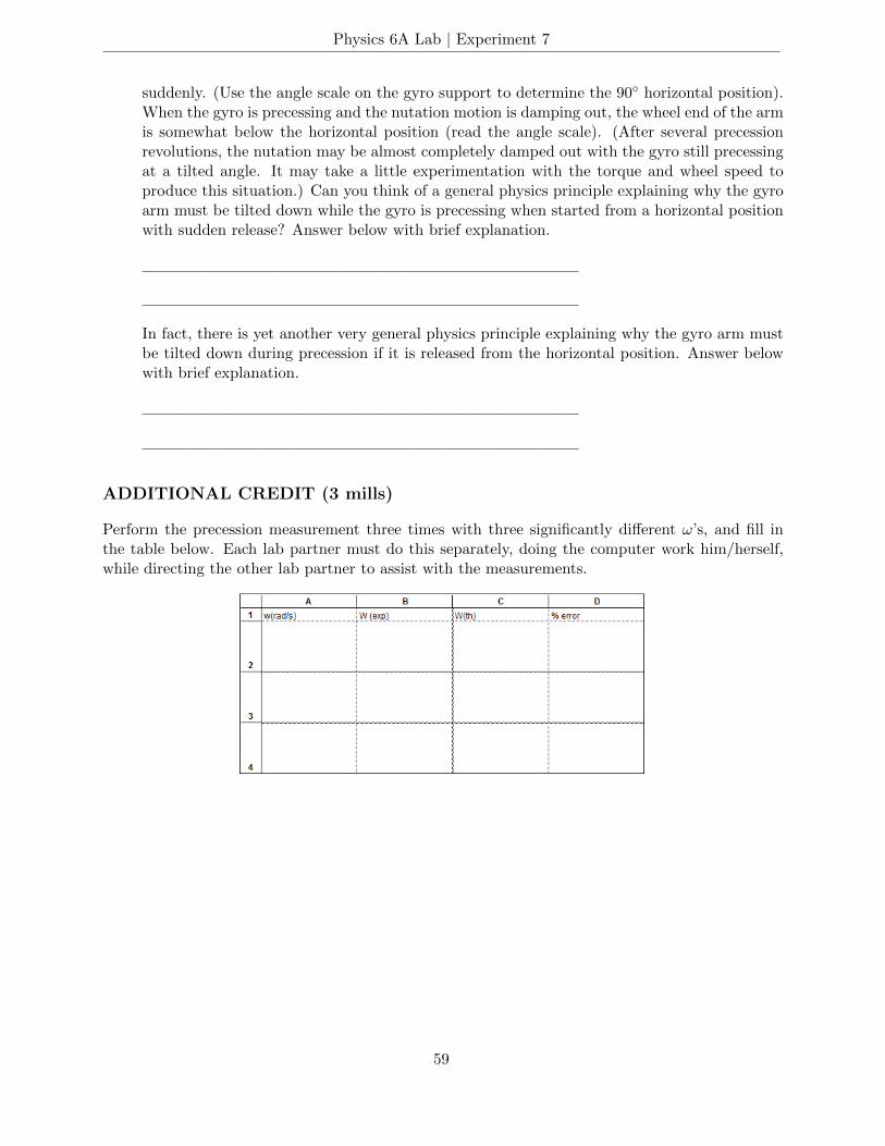
Physics 6A Lab | Experiment 7
suddenly. (Use the angle scale on the gyro support to determine the 90 horizontal position).When the gyro is precessing and the nutation motion is damping out, the wheel end of the armis somewhat below the horizontal position (read the angle scale). (After several precessionrevolutions, the nutation may be almost completely damped out with the gyro still precessingat a tilted angle. It may take a little experimentation with the torque and wheel speed toproduce this situation.) Can you think of a general physics principle explaining why the gyroarm must be tilted down while the gyro is precessing when started from a horizontal positionwith sudden release? Answer below with brief explanation.
In fact, there is yet another very general physics principle explaining why the gyro arm mustbe tilted down during precession if it is released from the horizontal position. Answer belowwith brief explanation.
ADDITIONAL CREDIT (3 mills)
Perform the precession measurement three times with three significantly different ω’s, and fill inthe table below. Each lab partner must do this separately, doing the computer work him/herself,while directing the other lab partner to assist with the measurements.
59


