Download - MULTIGRID ALGORITHMS - Freeebrary.free.fr/Mesh Generation/Wesseling - Introduction to... · 8 MULTIGRID ALGORITHMS 8.1. Introduction ... The linear multigrid algorithm follows easily

8 MULTIGRID ALGORITHMS

8.1. Introduction

The order in which the grids are visited is called the multigrid schedule. Several schedules will be discussed. All multigrid algorithms are variants of what may be called the basic multigrid algorithm. This basic algorithm is nonlinear, and contains linear multigrid as a special case.

The most elegant description of the basic multigrid algorithm is by means of a recursive formulation. FORTRAN does not allow recursion, thus we also present a non-recursive formulation. This can be done in many ways, and various flow diagrams have been presented in the literature. If, however, one constructs a structure diagram not many possibilities remain, and a well structured non-recursive algorithm containing only one goto statement results. The decision whether to go to a finer or to a coarser grid is taken in one place only.

8.2. The basic two-grid algorithm

Preliminaries

Let a sequence (G k: k = 1,2, . . . , K 1 of increasingly finer grids be given. Let Uk be the set of grid functions Gk --* R on Gk; a grid function uk € U k stands for m functions in the case where we want to solve a set of equations for rn unknowns. Let there be given transfer operators Pk: Uk-' + Uk (prolongation) and Rk: Uk-' -, Uk (restriction). Let the problem to be solved on Gk be denoted by

Lk(uk) = bk (8.2.1)

The operator Lk may be linear or non-linear. Let on every grid a smoothing algorithm be defined, denoted by S (u, v , f, v, k). S changes an initial guess uk into an improved approximation vk with right-hand sidefk by Vk iterations with a suitable smoothing method. The use of the same symbol uk for the sol-

The basic two-grid algorithm 169

ution of (8.2.1) and for approximations of this solution will not cause con- fusion; the meaning of u' will be clear from the context. On the coarsest grid G' we sometimes wish to solve (8.2.1) exactly; in general we do not wish to be specific about this, and we write S(u, u, f , a , 1) for smoothing or solving on G'.

The nonlinear two-grid algorithm

Let us first assume that we have only two grids G' and Gk-' . The following algorithm is a generalization of the linear two-grid algorithm discussed in Section 2.3. Let some approximations C k of the solution on G' be given. How C k may be obtained will be discussed later. The non-linear two-grid algorithm is defined as follows. Let f'= bk .

Subroutine TG (C, u, f , k ) comment nonlinear two-grid algorithm begin

S(C, u * f , y , k )

Choose Ck-', sk-1

S(4 u,f, a t k - 1)

S(u, u,f , PI k )

r k =p - L'(U')

p-l= L&-l(Ck-l ) + s'- 1Rk- '#

u k = U'+ (l/s'-l)Pk(U'-' - Zik-l)

end of TG

A call of TG gives us one two-grid iteration. The following program performs ntg two-grid iterations:

Choose I lk p = b ' for i = 1 step 1 until ntg do

TG (C, u , f , k ) C = u

od

Discussion

Subroutine TG is a straightforward implementation of the basic multigrid principles discussed in Chapter 2, but there are a few subtleties involved.

170 MuItigrid algorithms

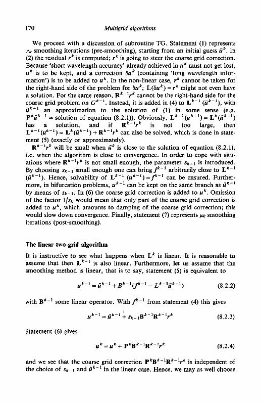
We proceed with a discussion of subroutine TG. Statement (1) represents Vk smoothing iterations (pre-smoothing), starting from an initial guess f i k . In (2) the residual rk is computed; rk is going to steer the coarse grid correction. Because 'short wavelength accuracy' already achieved in u Ir must not get lost, uk is to be kept, and a correction 6uk (containing 'long wavelength information') is to be added to uk. In the non-linear case, rk cannot be taken for the right-hand side of the problem for 6uk; L(6uk) = rk might not even have a solution. For the same reason, Rk-'rk cannot be the right-hand side for the coarse grid problem on Gk-' . Instead, it is added in (4) to Lk-' ( f i k - ' ) , with

an approximation to the solution of (1) in some sense (e.g. - solution of equation (8.2.1)). Obviously, Lk-' (uk-') = Lk( f ik - ' )

has a solution, and if Rk-'rk is not too large, then ) = Lk(Ck- ' ) + Rk-'rk can also be solved, which is done in state-

ment ( 5 ) (exactly or approximately). Rk-'rk will be small when I lk is close to the solution of equation (8.2.1),

i.e. when the algorithm is close to convergence. In order to cope with situ- ations where Rk-'rk is not small enough, the parameter sk -1 is introduced. By choosing sk- 1 small enough one can bring I"-' arbitrarily close to Lk-' (iik-'). Hence, solvability of Lk-' (uk- ' ) =fk-' can be ensured. Further- more, in bifurcation problems, uk-l can be kept on the same branch as f i k - ' by means of S k - I . In (6) the coarse grid correction is added to uk. Omission of the factor 1 / sk would mean that only part of the coarse grid correction is added to uk, which amounts to damping of the coarse grid correction; this would slow down convergence. Finally, statement (7) represents pk smoothing iterations (post-smoothing).

f i k - 1

p k f i k - 1 I

L k - 1 k - 1 (u

The linear two-grid algorithm

It is instructive to see what happens when Lk is linear. It is reasonable to assume that then L"-' is also linear. Furthermore, let us assume that the smoothing method is linear, that is to say, statement (5 ) is equivalent to

1 U k - l - - f i k - 1 + ~ k - l C f k - l - ~ k - l f i k - 1 (8.2.2)

with Bk-' some linear operator. With p-' from statement (4) this gives

Statement (6) gives

(8.2.4)

and we see that the coarse grid correction PkBk-lRk-'rk is independent of the choice of Sk-1 and Ik - ' in the linear case. Hence, we may as well choose

The basic two-grid algorithm 171

sk-l = 1 and tik-' = 0 in the linear case. This gives us the following linear two-grid algorithm.

Choice of and sk-1

There are several possibilities for the choice of J k - ' . One possibility is

U k (8.2.5) z k - 1 - - R k - 1

where Rk-' is a restriction operator which may or may not be the same as

With the choice sk-1 = 1 this gives us the first non-linear multigrid algorithm that has appeared, the FAS (full approximation storage) algorithm proposed by Brandt (1977). The more general algorithm embodied in subroutine TG, containing the parameter sk-1 and leaving the choice of &-I open, has been proposed by Hackbusch (1981, 1982, 1985). In principle it is possible to keep Ck-1 fixed, provided it is sufficiently close to the solution of Lk-' (uk - ' ) = b k - ' . This decreases the cost per iteration, since Lk-' ( , j k - ' ) needs to be evaluated only once, but the rate of convergence may be slower than with Zh-' defined by (5 ) . We will not discuss this variant. Another choice of

Hackbusch (1981, 1982, 1985) gives the following guidelines for the choice of iik-' and the parameter sk-1. Let the non-linear equation Lk-'(uk-') =f'-' be solvable for l l J k - ' 11 < pk-1. Let 1) Lk- ' (Ck- ' ) 11 < pk-42. Choose sk-1 such that 11 sk-lRk-lrh (1 < p k - 1 / 2 , for example:

Rk-1

is provided by nested iteration, which will be discussed later. ,jh-1

sk- 1 = i p k - I/ 11 Rk-'rk 11. (8.2.6)

Then I I f - ' 11 < p k - I , so that the coarse grid problem has a solution.

172 Multigrid algorithms

8.3. The basic multigrid algorithm The recursive non-linear multigrid algorithm

The basic multigrid algorithm follows from the two-grid algorithm by replacing the coarse grid solution statement (statement (5) in subroutine TG) by Y k multigrid iterations. This leads to

Subroutine MG1 (i, u, f , k , y)

comment recursive non-linear multigrid algorithm begin

i f ( k eq 1) then

else w, u , f , * , k )

S(1, u , f , v , k ) rk =f' - L'(u~) Choose ik-', sk-1

f"-' = Lk- l ( ik - I ) + s ~ - ~ R ~ - ~ ~ ~ for i = 1 step 1 until yk do

MG1 ( C , u , f , k - 1 , ~ ) ik-I - U k - l -

od u k = U k + ( I / s k - l ) P k ( U k - ' - i k - ' )

S(U, u, f, P, k ) endif

end of MGl

After our discussion of the two-grid algorithm, this algorithm is self- explanatory. According to our discussion of the choice of ik-' in the preceding section, statement (7) could be deleted or replaced by something else.

The following program carries out nmg multigrid iterations, starting on the finest grid GK:

Program I: Choose iK fK = b K for i = 1 step 1 until nmg do

MG1 (C, u , f , K , Y) i K = U K

Od

The basic rnultigrid algorithm 173

The recursive linear multigrid algorithm

The linear multigrid algorithm follows easily from the linear two-grid algorithm LTG:

Subroutine LMG (6, u, f, k ) comment recursive linear multigrid algorithm begin

if ( k = 1) then

else S@, u, f, - , k )

S(i, u,f9 v , k ) rk = f k - ~ k u k fk-1 =Rk-lrk z k - l = 0

for i = 1 step 1 until y k do LMG (ij, u,J, k - 1) i jk- l= k - 1 U

od U k = U k + pkuk-1

S(u, u, f , p, k) endif

end LMG

Multigrid schedules

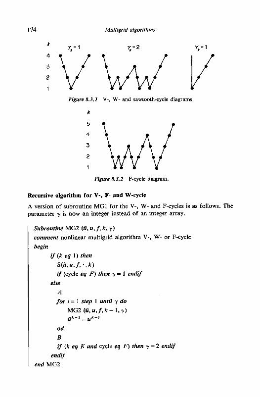
The order in which the grids are visited is called the multigrid schedule or multigrid cycle. If the parameters yk, k = 1,2, . . . , K - 1 are fixed in advance we have a fixed schedule; if - f k depends on intermediate computational results we have an adaptive schedule. Figure 8.3.1 shows the order in which the grids are visited with yk = 1 and yk = 2, k = 1,2, ..., K- 1, in the case K = 4. A dot represents a smoothing operation. Because of the shape of these diagrams, these schedules are called the V-, W- and sawtooth cycles, respectively. The sawtooth cycle is a special case of the V-cycle, in which smoothing before coarse grid correction (pre-smoothing) is deleted. A schedule intermediate between these two cycles is the F-cycle. In this cycle coarse grid correction takes place by means of one F-cycle followed by one V-cycle. Figure 8.3.2 gives a diagram for the F-cycle, with K = 5 .

174 Multigrid algorithms ‘ v ~ k v 2

1

Figure 8.3.1 V-, W- and sawtooth-cycle diagrams.

k

Figure 8.3.2 F-cycle diagram.

Recursive algorithm for V-, F- and W-cycle

A version of subroutine MG1 for the V-, W- and F-cycles is as follows. The parameter y is now an integer instead of an integer array.

Subroutine MG2 (fi, u, f , k , y) comment nonlinear multigrid algorithm V-, W- or F-cycle begin

i f (k eq 1) then S(& u, f, ., k ) if (cycle eq F) then y = 1 endif

else A for i = 1 step 1 until y do

MG2 ( & u , f , k - 1 , ~ ) j p - 1 -

od B if ( k eq K and cycle eq F ) then y = 2 endif

endif I endMG2

The basic multigrid algorithm 175

Here A and B represent statements (2) to (5) and (8) and (9) in subroutine MG1. The following program carries out nmg V-, W- or F-cycles.

Program 2: Choose z Z K

if (cycle eq W or cycle eq F) then y = 2 else y = 1 for i = 1 step 1 until nmg do

f K = b K

MG2 (6, u, f, K , y) i K = U K

od

Adaptive schedule

An example of an adaptive strategy is the following. Suppose we do not carry out a fixed number of multigrid iterations on level Gk, but wish to continue to carry out multigrid interactions, until the problem on Ck is solved to within a specified accuracy. Let the accuracy requirement be

with 6 E (0 , l ) a parameter. At first sight, a more natural definition of ck would seem to be ck = 6 I l f I ( .

Since J" does not, however, go to zero on convergence, this would lead to skipping of coarse grid correction when uk+' approaches convergence. Analysis of the linear case leads naturally to condition (8.3.1). An adaptive multigrid schedule with criterion (8.3.1) is implemented in the following algorithm. In order to make the algorithm finite, the maximum number of multigrid iterations allowed is y.

Subroutine MG3 (Iz, u, f, k ) ' comment recursive nonlinear rnultigrid algorithm with adaptive I schedule

begin I

if (k eq 1) then S(f i , u, f, - , k )

else A

I fk- l=I(r*(I-&k

I ck-1 = 6sk-lll rkll I n k - l =


od B

endif end MG3

Here A and B stand for the same groups of statements as in subroutine MG2. The purpose of statement (1) is to allow the possibility that the required accuracy is already reached by pre-smoothing on Gk, so that coarse grid correction can be skipped. The following program solves the problem on G K within a specified tolerance, using the adaptive subroutine MG3:

Program 3: Choose rl f K = b K ; &K=tOl*I)bK(I; t~=(IL~(fi~)-b~I( -&K

n = nmg while ( t K > 0 and n 2 0) do

MG3(rl, u, f, K ) C K = U K

n = n - 1 fK = 11 L K ( ~ K ) - bKII - &K

od

The number of iterations is limited by nmg.

Storage requirements

Let the finest grid G K be either of the vertex-centred type given by (5.1.1) or of the cell-centred type given by (5.1.2). Let in both cases na = nLK) = ma . 2K. Let the coarse grids G', k = K - 1 , K - 2, . . . , 1 be constructed by successive doubling of the mesh-sizes h, (standard coarsening). Hence, the number of grid-points N k of Gk is

d

a=l Nk = IT (1 + m a - 2') = k f 2 k d (8.3.2)


in the vertex-centred case, with

and

Nk = M2kd (8.3.3)

in the cellcentred case. In order to be able to solve efficiently on the coarsest grid GI it is desirable that m, is small. Henceforth, we will not distinguish between the vertex-centred and the cell-centred case, and assume that Nk is given by (8.3.3).)

It is to be expected that the amount of storage required for the computa- tions that take place on Gk is given by clNk, with CI some constant independent of k. Then the total amount of storage required is given by

(8.3.4)

Hence, as compared to single grid solutions on GK with the smoothing- method selected, the use of multigrid increases the storage required by a factor of 2d/(2d - l), which is 413 in two and 817 in three dimensions, so that the additional storage requirement posed by multigrid seems modest.

Next, suppose that semi-coarsening (cf. Section 7.3) is used for the construction of the coarse grids Gk, k < K. Assume that in one coordinate direction the mesh-size is the same on all grids. Then

N~ = ~ 2 K + k ( d - l ) (8.3.5)

and the total amount of storage required is given by

(8.3.6)

Now the total amount of storage required by multigrid compared with single grid solution on GK increases by a factor 2 in two and 413 in three dimensions. Hence, in two dimensions the storage cost associated with semi-coarsening multigrid is not negligible.

Computational work

We will estimate the computational work of one iteration with the fixed schedule algorithm MG2. A close approximation of the computational work wk to be performed on Gk will be Wk=czNk, assuming the number of pre- and post-smoothings V k and pk are independent of k, and that the operators


L' are of similar complexity (for example, in the linear case, Lk are matrices of equal sparsity). More precisely, let us define wk to be all computing work involved in MG2 ( G , u, $, k), except the recursive call of MG2. Let w k be all work involved in MG2 (&u, f, k) . Let yk = y, k = 2,3, ..., K- 1, in subroutine MG2 (e.g., the V- or W-cycles). Assume standard coarsening. Then

Wk=C2kf2kd+YWk-l (8.3 -7)

One may write

).'.)) (8.3.8)

with 7 = ~ / 2 ~ . Here we have assumed Wl = c ~ M y 2 ~ . This may be inaccurate, since W, does not depend on y in reality, and, moreover, often a solution close to machine accuracy is required on GI, for example when the problem is singular (e.g. with Neumann boundary conditions.) Since WI is small anyway, this inaccuracy is, however, of no consequence. From (8.3.8) it follows that

WK = C2M2Kd(l+ y(2-d + y ( 2 4 + * * - + y2('-K)d = C ~ N K ( ~ -k 7 + 7' 4- ** . 4- TK-')

(8.3.9)

where i V K = WK/ (c2NK). If 7 c 1 one may write

F K < W = 1/(1 -7) (8.3.10)

The following conclusions may be drawn from (8.3.8), (8.3.9) and (8.3.10). @K is the ratio of multigrid work and work on the finest grid. The bulk of the work on the finest grid usually consists of smoothing. Hence, RK- 1 is a measure of the additional work required to accelerate smoothing on the finest grid GK by means of multigrid.

If 7 2 1 the work WK is superlinear in the number of unknowns Nx, because from (8.3.8) it follows that

Hence, if 7 > 1 WK is superlinear in NK. If 7 = 1 equation (8.3.8) gives

again showing superlinearity of WK. If 7 < 1 equation (8.3.10) gives


so that WK is linear in NK. It is furthermore significant that the constant of proportionality cz/(1 - 4) is small. This because c2 is just a little greater than the work per grid point of the smoothing method, which is supposed to be a simple iterative method (if not, multigrid is not applied in an appropriate way). Since an (perhaps the main) attractive feature of multigrid is the possibility to realize linear computational complexity with small constant of proportionality, one chooses 7 < 1, or y < 2d. In practice it is usually found that y > 2 does not result in significantly faster convergence. The rapid growth of WK with y means that it is advantageous to choose y Q 2, which is why the V- and W-cycles are widely used.

The computational cost of the F-cycle may be estimated as follows. In Figure 8.3.3 the diagram of the F-cycle has been redrawn, distinguishing between the work that is done on G' preceding coarse grid correction (pre- work, statements A in subroutine MG2) and after coarse grid correction (post-work, statements B in subroutine MG2). The amount of pre- and post- work together is C Z M ~ ~ ~ , as before. It follows from the diagram, that on G k the cost of pre- and post-work is incurred j k times, with j k = K - k+ 1 , k = 2,3, ..., K, and j1= K - 1. For convenience we redefine j l = K , bearing our earlier remarks on the inaccuracy and unimportance of the estimate of the work on G' in mind. One obtains

d

K

k = l W K = C Z M C (K-k+ 1)2kd (8.3.14)

We have

(8.3.15) 2d

k=I (Zd - (2d - K ( K + 1)d C k2kd= [K(2d - 1) - 11 + -

as is checked easily. It follows that

k

Figure 8.3.3 F-cycle (0 pre-work, 0 post-work).


Table 8.3.1. Values of W, standard coarsening

~

d 2 3

V-cycle 413 817 F-cycle 1619 64/49 W-cycle 2 413 y = 3 4 815

so that

Table 8.3.1 gives Was given by (8.3.10) and (8.3.16) for a number of cases. The ratio of multigrid over single grid work is seen to be not large, especially in three dimensions. The F-cycle is not much cheaper than the W-cycle. In three dimensions the cost of the V-, F- and W-cycles is almost the same.

Suppose next that semi-coarsening is used. Assume that in one coordinate direction the mesh-size is the same on all grids. The number of grid-points Nk of Gk is given by (8 .3 .5) . With Yk = 7, k = 2 , 3 , ..., K - 1 we obtain

Hence WK is given by (8 .3 .8) and W by (8 .3 .10) with 7 = ~ / 2 ~ - l . For the F-cycle we obtain

Hence

Table8.3.2. Values of @, semi-coarsening

d 2 3

V-cycle 2 41 3 F-cycle 4 1619 W-cycle - 2

4 y = 3 -

Nesfed iteration 181

Table 8.3.2 gives @ for a number of cases. In two dimensions y = 2 or 3 is not useful, because + 2 1. It may happen that the rate of convergence of the V-cycle is not independent of the mesh-size, for example if a singular pertur- bation problem is being solved (e.g. convection-diffusion problem. with E 4 I) , or when the solution contains singularities. With the W-cycle we. have + = 1 with semi-coarsening, hence p k = K. In practice, K is usually not greater than 6 or 7, so that the W-cycle is still affordable. The F-cycle may be more efficient.

Work units

The ideal computing method to approximate the behaviour of a given physical problem involves an amount of computing work that is proportional to the number and size of the physical changes that are modeled. This has been put forward as the ‘golden rule of computation’ by Brandt (1982). As has been emphasized by Brandt in a number of publications, e.g. Brandt (1977, 1977a, 1980, 1982), this involves not only the choice of methods to solve (8.2.1)’ but also the choice of the mathematical model and its discretization. The discretization and solution processes should be intertwined, leading to adaptive discretization. We shall not discuss adaptive methods here, but regard (8.2.1) as given. A practical measure of the minimum computing work to solve (8.2.1) is as follows. Let us define one work unit (WU) as the amount of computing work required to evaluate the residual L K ( u K ) - bK of Equation (8.2.1) on the finest grid G K . Then it is to be expected that (8.2.1) cannot be solved at a cost less than a few WU, and one should be content if this is realized. Many publications show that this goal can indeed be achieved with multigrid for significant physical problems, for example in computational fluid dynamics. In practice the work involved in smoothing is by far the domi- nant part of the total work. One may, therefore, also define one work udit, following Brandt (1977), as the work involved in one smoothing iteration on the finest grid GK. This agrees more or less with the first definition only if the smoothing algorithm is simple and cheap. As was already mentioned, if this is not the case multigrid is not applied in an appropriate way. One smoothing iteration on G k then adds 2d‘k-K’ WU to the total work. It is a good habit, followed by many authors, to publish convergence histories in terms of work units. This facilitates comparisons between methods, and helps in developing and improving multigrid codes.

8.4. Nested iteration

The algorithm

Nested iteration, also called full multigrid (FMG, Brandt (1980, 1982)) is based on the following idea. When no a priori information about the solution


is available to assist in the choice of the initial guess J K on the finest grid GK, it is obviously wasteful to start the computation on the finest grid, as is done by subroutines MGi, i = 1,2,3 of the the preceding section. With an unfortu- nate choice of JK, the algorithm might even diverge for a nonlinear problem. Computing on the coarse grids is so much cheaper, thus it is better to use the coarse grids to provide an informed guess for JK. At the same time, this gives us a choice for J k , k < K. Nested iteration is defined by the following algorithm.

(3) (4)

Program I comment nested iteration algorithm Choose J1 S( f i , f i , f , *, 1) for k = 2 step 1 until K do

I l k = p k f i k - I

for i = 1 step 1 until f k do MG ( J , u, f, k ) J k = u k

od od

Of course, the value of 'yk inside MG may be different from t r .

Choice of prolongation operator

The prolongation operator F k does not need to be identical to P k . In fact, there may be good reason to choose it differently. As will be discussed in Section 8.6, it is often advisable to choose f i k such that

mp> mc (8.4.1)

where mp is the order of the prolongation operator as defined in Section 5.3, and rn, is the order of consistency of the discretizations Lk, here assumed to be the same on all grids. Often m, = 2 (second-order schemes). Then (8.4.1) implies that pk is exact for second-order polynomials.

Note that nested iteration provides i ik; this is an alternative to (8.2.5). As will be discussed in the next section, if MG converges well then the

nested iteration algorithm results in a uK which differs from the solution of (8.2.1) by an amount of the order of the truncation error. If one desires, the accuracy of uK may be improved further by following the nested iteration algorithm with a few more multigrid iterations.

Nested iteration 183

Computational cost of nested iteration

Let y k = i , k = 2,3, ..., K, in the nested iteration algorithm, let w k be the work involved in MG (ii,u, f , k ) , and assume for simplicity that the (negligible) work on G' equals W I . Then the computational work Wni of the nested iteration algorithm, neglecting the cost of p k , is given by

K

k = l wni= i w k (8.4.2)

Assume inside MG y k = y, k = 2,3, ..., K and let + = y/2d < 1 . Note that y and 9 may be different. Then it follows from (8.3.10) that

(8.4.3)

Defining a work unit as 1 WU = CZNK, i.e. approximately the work of (v + p ) smoothing iterations on the finest grid, the cost of a nested iteration is

(8.4.4)

Table 8.4.1 gives the number of work units required for nested iteration for a number of cases. The cost of nested iteration is seen to be just a few work units. Hence the fundamental property, which makes multigrid methods so attractive: multigrid methods can solve many problems to within truncation error at a cost of CN arithmetic operations. Here N is the number of unknowns, and c is a constant which depends on the problem and on the multigrid method (choice of smoothing method and of the parameters Yk, p k , y k ) .

If the cost of the residual bK - L K ( u K ) is dN, then c need not be larger than a small multiple of d. Other numerical methods for elliptic equations require O(Na) operations with a > 1, achieving O(N In N) only in special cases (e.g. separable equations). A class of methods which is competitive with multigrid for linear problems in practice are preconditioned conjugate gradient methods. Practice and theory (for special cases) indicate that these require O(N") operations, with ar=5/4 in two and a = 9 / 8 in three dimensions. Comparisons will be given later.

Table 8.4.2. Computational cost of nested iteration in work units; f = 1

d

Y 2 3

1 16/9 64/49 2 8/3 48/21


8.5. Rate of convergence of the multigrid algorithm

Preliminaries

For a full treatment of multigrid convergence theory, see Hackbusch (1985). See also Mandel et al. (1987). Here only an elementary introduction is presented, following the framework developed by Hackbusch (1985).

The problem to be solved

is assumed to be linear. Two-grid convergence theory has been discussed in Section 6.5. We will extend this to multiple grids. \ I - I\ will denote the Euclidean norm.

The smoothing and approximation properties

The smoothing method is assumed to be linear and of the type discussed in Section 4.1, with iteration matrix Sk on grid Gk, k = 2,3, ..., K. It is assumed that on G' exact solution takes place. The smoothing and approximation properties are defined as follows, cf. Definitions 6.5.1 and 6.5.2.

Definition 8.5.1. Smoothing property. S k has the smoothing property if there exist a constant CS and a function g ( v ) independent of hk such that

11 Lk(Sk)"( ( < Cshk2"T(v), g ( v ) + O for v + 00 (8.5.2)

where 2m is the order of the partial differential equation to be solved.

Definition 8.5.2. Approximation property. The approximation property holds if there exists a constant CA independent of h k such that

(8.5.3)

where 2m is the order of the differential equation to be solved.

The multigrid iteration matrix

The multigrid algorithm is defined by subroutine LMG of Section 8.3. Let V k = v, pk = p and yk = y be independent of k. The error ek is defined as e k = uk - (L")-'P. The error ek and e: before and after execution of LMG (fi ,u, f , k ) satisfies

e! = Q k ( v , p)ek (8.5.4)

Rate of convergence of the multigrid algorithm 185

with Qk the k-grid iteration matrix. Qk is given by:

Theorem 8.5.1. The iteration matrix Q k ( p , v) of LMG (C, u, J, k ) satisfies

Q2h v ) = Q2h v) (8.5.5a)

Q k ( p , v) = Q"(p, v ) + (Sk)pPk(Qk-')y(Lk-')-lRk-' L (Sky (8.5.5b)

is the iteration matrix of method LTG of Section 8.2.

Proof. From (6.5.11) it follows that Q k ( p , v) is the iteration matrix of LTG (fi, u, f, k). Equation (8.5.5a) is obviously true. Equation (8.5.5b) is proved by induction. Let e;", efA1, ez"/f' and e!+' be the error on Gk+' before LMG (fi, u, f, k), after pre-smoothing, after coarse grid correction and after post-smoothing, respectively. We have

(Sk+')uegk+l (8.5.6)

The coarse grid problem to be solved is

Lkuk = - RkLk+'efA' (8.5.7)

with initial guess uk = 0. Hence the initial error e; equals minus the exact solution on Gk, i.e. e; = (Lk)-lRkLk+lefA1. After coarse grid correction the error on Gk is (Qk)ye,k. Hence the coarse grid correction is given by [ - I + (Qk)y)e;. Therefore

(8.5.9)

Combining (8.5.6), (8.5.8) and (8.5.9) gives (8.5.5b) with k replaced by k + 1, which completes the proof. 0

Rate of convergence

We will prove that the rate of convergence of LMG is independent of the mesh-size only for p = 0 (no post-smoothing). For the more general case, which is slightly more complicated, we refer to Hackbusch (1985).

186 Muttigrid algorithms

Lemma 8.5.1. Let the smoothing property hold, and assume that there exists a constant c, independent of k such that

Then

Proof. It has been shown in Theorem 6.5.2 that, if Sk has the smoothing property, then the smoothing method is convergent. Hence we can choose v such that

II (sky II < 1 (8.5.12)

and

Using (8.5.10) and (8.5.12), (8.5.11) follows. 0

It will be necessary to study the following recursive inequality

For this we have the following Lemma.

Lemma 8.5.2. Assume Cy > 1. If

then any solution of (8.5.13) is bounded by

t k < z < 1

where z is related to < by

{ = z - C z Y

(8.5.13)

(8.5.14)

(8.5.15)

(8.5.16)

Rate of convergence of the multigrid algorithm 187

and z satisfies

ZQ- y r 7 - 1

(8.5.17)

Proof. We have {k Q Zk, with Zk defined by

Since ( z k ) is monotonically increasing, we have zk < z, with z the smallest solution of (8.5.16). Consider f ( z ) = z - Czy. The maximum of f ( z ) is reached in z = z* = ( 7 ~ ) - "h-- < 1, and f ( z* ) = f . For { < f Equation (8.5.16) has a solution z Q z* < 1. We have

which gives (8.5.17). 0

Theorem8.5.2. Rate of convergence of linear multigrid method. Let the smoothing and approximation properties (8.5.2) and (8.5.3) hold. Assume y 2 2. Let P k satisfy (8.5.10) and

11 Pkuk-l I( < Cp 11 uk-l 11, Cp independent of k. (8.5.19)

Let f < (0,l) be given. Then there is a number i independent of K such that the iteration matrix Q K ( O , V ) defined by Theorem 8.5.1 satisfies

if v 2 i .

Proof. we have

Q K is defined by the recursion (8.5.5). According to Theorem 6.5.1

II Q k < v , 0) II Q CSCAr l (V ) (8.5.21)

Choose a number r < ((I, f ) with f satisfying (8.5.14) and a number i such that

C S C A r l ( V ) < r, v 2 (8.5.22)

and that (8.5.12) is satisfied for Y 2 i . From (8.5.5), (8.5.12), (8.5.19) and Lemma 8.5.1 it follows that

r k < r -k cpll-Icp(l -k f ) Q f -k crZ-1 (8.5.23)


with C = 2C,c, and { k = 1 1 Q k ( O , v) 11. The recursion (8.5.23) has been ana- lyzed in Lemma 8.5.2. It follows that

< k G L !:< 1, k = 2 , 3 ,..., K (8.5.24) 7 - 1

If necessary, increase v such that !: < [(y - 1)/7] f. 0

This theorem works only for y 2 2. Hence the V- and F-cycles are not included. For self-adjoint problems, a similar theory is available for the V-cycle (Hackbusch 1985, Mandel, et al. 1987), which naturally includes the F-cycle.

The difficult part of multigrid convergence theory is to establish the smoothing and approximation properties. (See the discussion in Section 6.5.)

Convergence theory for the non-linear multigrid algorithm MG is more difficult than for LMG, of course. Hackbusch (1985) gives a global outline of a non-linear theory. A detailed analysis has to depend strongly on the nature of the problem. Reusken (1988) and Hackbusch and Reusken (1989) give a complete analysis for the following class of differential equations in two dimensions

with g non-linear, g’( t ) 2 0, Vt. In general it is difficult to say in advance how large V should be. Practical

experience shows that quite often with V = 1, 2 or 3 one already has f < 0.1, even with the Vcycle. Defining a work unit to be the cost of one smoothing on the finest grid, it follows that quite often with multigrid methods the cost of gaining a decimal digit accuracy is just a few work units, independent of the mesh-size of the finest grid.

Exercise 8.5.1. Consider the one-dimensional case, and define Pk by (5.3.1). Show that (8.5.10) and (8.5.19) are satisfied with c, = 1, C, = (312)”’.

8.6. Convergence of nested iteration

For a somewhat more extensive analysis of the convergence of nested iteration, see Hackbusch (1985), on which this section leans heavily.

Preliminaries

Let the (non-linear) differential equation to be solved be denoted by

L(u) = b (8.6.1)

Convergence of nested iteration 189

and let the discrete approximation on the grids Gk be denoted by

L k ( U k ) = B k (8.6.2)

Define the global discretization error ek by

(8.6.3) k E k = uk - (u )

where ( u ) Ir indicates the trivial restriction of u to Gk:

( U ) f = U ( X i ) (8.6.4)

Let the order of the discretization error of Lk be m, k = 1,2, ..., K , i.e.

I I E ~ ( ( <arnk, k = 1 , 2 ,..., K (8.6.5)

where 11 * 1) is a norm which is not necessarily Euclidean and which we do not specify further; rn depends on the choice of 11 - 1 1 . In (8.6.5) we assume that 2-* is proportional to the step sizes on Gk, i.e. the step sizes on Gk are obtained from those on Gk-' by halving.

Recursion for the error of nested iteration

Denote the result of statement (2) in the nested iteration Algorithm (para- graph 1 of Section 8.4) by u& and the result of Statement (4) by tZk. Let < be an upper bound for the contraction number of the multigrid algorithm, and let T k = T , k = 2 , 3 ,..., K. Then

(uk is the solution of (8.6.2)). We have, for k = 2,

defining

Estimates for C(k) will be provided later. It follows that

(8.6.8)

(1 ri2 - u2 I( < C(2)P (8.6.9)


For general k,

assuming that

(IpkII <Cp, k = 2 , 3 ,..., K (8.6.11)

Let Bk = 11 ik - uk 11, then (8.6.6), (8.6.9) and (8.6.10) give

Hence

We will provide estimates of C(k) of the form

C(k) < Cp2-pk

Substitution in (8.6.13) gives

K - 2 BK < f'€p2-PK C rk , r=2Pl'Cp

k=O

Assume

r = 2 p f f C p c 1

(8.6.13)

(8.6.14)

(8.6.15)

(8.6.16)

Then (8.6.15) gives the following result

Accuracy of prolongation in nested iteration

We now estimate C(k) . We want to compare iik - uk with the discretization error ek. Suppose we have the following asymptotic expansion for ek


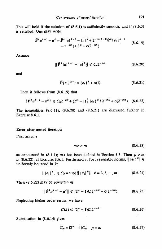
This will hold if the solution of (8.6.1) is sufficiently smooth, and if (8.6.5) is satisfied. One may write

Assume

11 P ( U ] k - l - (u) 11 f cu2-pk (8.6.20)

and

Then it follows from (8.6.19) that

11 P k U k - 1 - uk 11 8 CU2-pk + (2" - 1) 11 (el) ' [I 2-mk + 0(2-"~) (8.6.22)

The inequalities (8.6.11), (8.6.20) and (8.6.21) are discussed further in Exercise 8.6.1.

Error after nested iteration

First assume

m p > m (8.6.23)

as announced in (8.4.1); mP has been defined in Section 5.3. Then p > m in (8.6.22), cf Exercise 8.6.1. Furthermore, for reasonable norms, 11 [el ] '(1 is uniformly bounded in k:

Then (8.6.22) may be rewritten as

(1 P u k - l - u q < (2m - 1)Cc2-"k + o(2-h) (8.6.25)

Neglecting higher order terms, we have

C(k) f (2" - 1)C,2-"k (8.6.26)

Substitution in (8.6.14) gives

= (2" - l)Cc, P = m (8.6.27)

192 Muitigrid algorithms

so that (8.6.17) becomes

11 cK - uK 1 1 < {Q" - 1 ) ~ , 2 - " ~ / ( 1 - r ) (8.6.28)

Comparison with (8.6.18) and (8.6.24) gives us the following theorem, noting that (8.6.16) becomes

r = 2"'r4CP < 1 (8.6.29)

Theorem 8.6.1. Error after nested iteration. If conditions (8.6.1 l), (8.6.18), (8.6.20), (8.6.23), (8.6.24) and (8.6.29) are fulfilled, then the error after nested iteration satisfies, neglecting higher order terms,

where

~ ( t , 7) = r'(2" - I)/ (1 - r ) (8.6.31)

This theorem says that after nested iteration the solution on GK is approxi- mated within D ( { , +) times the discretization error. How large is D({ , +)? Assume C, < 2, which is usually the case, cf. Exercise 8.6.1. Assume that m = 2 (second-order discretization). Then Condition (8.6.29) becomes

{+< 118 (8.6.32)

From (8.6.31) it follows with m = 2 that D ( { , 7) < 1 for {+ < 1/7. Hence, if we want the error after nested iteration to be smaller than the discretization error + should satisfy

+ a -In 8/ln ( (8.6.33)

Taking r = 1/4 as a typical value of the multigrid contraction number, + = 2 is sufficient. This shows that with nested iteration, multigrid gives the discrete solution within truncation error accuracy in a small number of work units, regardless of the mesh size.

Less accurate prolongation

For second-order accurate discretizations (rn = 2) equation (8.6.23) implies that pk should be exact for polynomials of degree at least 2. For second-order differential equations, however, the multigrid method requires only prolonga- tions that are exact for polynomials of degree 1 (i.e. mp = 2, since usually mR 2 1, so that mp + mR > 2 is satisfied). We will now investigate the


accuracy of the nested iteration result if mg = 2. Again assuming rn = 2, Equation (8.6.22) can be written as

11 e k U k - ' - U k 11 < e22-2k + o ( 2 - Z k ) (8.6.34)

so that (8.6.14) holds with p = 2, neglecting higher order terms. Assuming

r = 2 2 r 9 ~ p < 1 (8.6.35)

Equation (8.6.17) gives us the following theorem.

Theorem 8.6.2. Error after nested iteration. If mp = 2 and if conditions (8.6.1 I), (8.6.20) (with p = 2) and (8.6.35) are satisfied and if m = 2 in (8.6.5) then the error after nested iteration satisfies, neglecting higher order terms,

This theorem shows that with m g = 2 after nested iteration the error is 0(2-2K), like the discretization error. Hence, it is also useful to apply nested iteration with Pk = P k (assuming mp = 2), avoiding the use of a higher order prolongation operator. There is, however, now no guarantee that the iteration error will be smaller than the discretization error.

Exercise 8.6.1. Let the one-dimensional vertex-centred prolongation operator p k be defined by

[ p k 7 = & [ - l 9 16 9 -11 (8.6.37)

Show that rnt=4. Define 11 * )I by

(8.6.38) j = O

and show (cf. 8.6.11))

11 f i k 11 < Cp = (41/32)'" (8.6.39)

Show that (8.6.20) holds with

cu=3Jzsup - p = 4 n o I dx4 d4U I ' (8.6.40)

Show that this implies (8.6.21).

194 Muftigrid algorithms

8.7. Non-recursive formulation of the basic multigrid algorithm

Structure diagram for fixed multigrid schedule

In FORTRAN, recursion is not allowed: a subroutine cannot call itself. The subroutines MG1,2,3 of Section 8.3 cannot, therefore, be implemented directly in FORTRAN. A non-recursive version will, therefore, be presented. At the same time, we will allow greater flexibility in the decision whether to go to a finer or to a coarser grid.

Various flow diagrams describing non-recursive multigrid algorithms have been published, for example in Brandt (1977) and Hackbusch (1985). In order to arrive at a well structured program, we begin by presenting a structure diagram. A structure diagram allows much less freedom in the design of the control structure of an algorithm than a flow diagram. We found basically only one way to represent the multigrid algorithm in a structure diagram (Wesseling 1988, 1990a). This structure diagram might, therefore, be called the canonical form of the basic multigrid algorithm. The structure diagram is given in Figure 8.7.1. This diagram is equivalent to Program 2 calling MG2 to do nmg multigrid iterations with finest grid GK in Section 8.3. The schedule is fixed and includes the V-, W- and F-cycles. Parts A and B are specified after subroutine MG2 in Section 8.3. Care has been taken that the program also works as a single grid method for K = 1.

FORTRAN implementation of while clause

Apart from the while clause, the structure diagram of Figure 8.7.1 can be expressed directly in FORTRAN. A FORTRAN implementation of a while clause is as follows. Suppose we have the following program

while (n(K) > 0) do Statement 1 n ( K ) = ... Statement 2

od

A FORTRAN version of this program is

10 if ( n ( K ) > 0) then Statement 1 n(K) = Statement 2 got0 10

endif


The goto statement required for the FORTRAN version of the while clause is the only goto needed in the FORTRAN implementation of the structure diagram of Figure 8.7.1. This FORTRAN implementation is quite obvious, and will not be given.

Structure diagram for adaptive multigrid schedule

Figure 8.7.2 gives a structure diagram for a non-recursive version of Program 3 of Section 8.3, using subroutine MG3 with adaptive schedule. To ensure that the algorithm is finite, the number of iterations on GK is limited by nmg and on Gk, k < K by y.

There is great similarity to the structure diagram for the fixed schedule. This is due to the fundamental nature of these structure diagrams. It is hard, if not impossible, to fit the algorithm into a significantly different structure diagram. The reason is that structure diagrams impose programming without goto. The flow diagrams of multigrid algorithms that have appeared show significant differences, even if they represent the same algorithm.

FORTRAN subroutine

The great similarity of the two structure diagrams means that it is easy to join them in one structure diagram. We will not do this, because this makes the basic simplicity of the algorithm less visible. Instead, we give a FORTRAN subroutine which incorporates the two structure diagrams (cf. Khalil and Wesseling 1991).

C

C

C

C

C

C C

C

C C

C

C C

C

C

Subroutine MG(ut,u,b,K,cycle,nmg,tol) Nonlinear multigrid algorithm including V-, W-, F- and adaptive cycles. Problem to be solved: L(u;K) = b(K) on grid G(K).

character cycle dimension ut( .),u( .),b( .)

ut (input: initial approximation. u (output): current solution. b (input): K (input): cycle (input): nmg (input):

right-hand-side on finest grid. number of finest grid. V,W,F or A, A gives adaptive cycle. fixed cycle: number of iterations. adaptive cycle: maximum number of iterations. accuracy requirement for adaptive cycle: to1 (input): I (L(u;K) - b(K) I C to1 * I b(K) I

dimension f(.),r(.),n,eps,t(l:K) f: right-hand-sides r: residuals

A

\ f k < o or n k eq o or k eq 1

T

I

I k = k + l

Figure 8.7.2 Structure diagram of non-recursive rnultigrid algorithm with adaptive schedule.

Multigrid algorithms I98

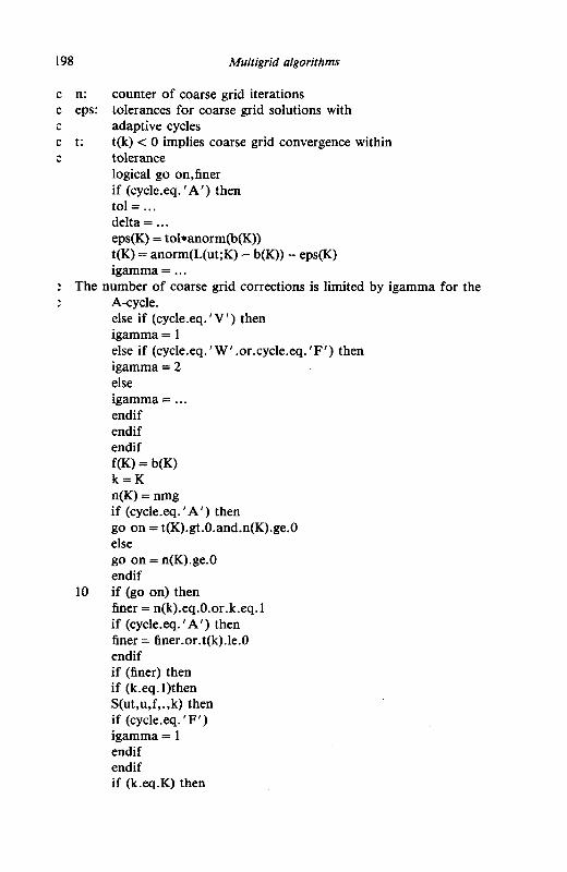
c n: c eps: C

c t: C

counter of coarse grid iterations tolerances for coarse grid solutions with adaptive cycles t(k) c 0 implies coarse grid convergence within tolerance logical go on,finer if (cycle.eq. ’A’) then to1 = ... delta = ... eps(K) = tol*anorm(b(K)) t(K) = anorm(L(ut;K) - b(K)) - eps(K) igamma = ...

: The number of coarse grid corrections is limited by igamma for the A-cycle. else if (cycle.eq.‘V’) then igamma = 1 else if (cycle.eq. ’ W’ .or.cycle.eq. IF’) then igamma = 2 else igamma = ... endif endif endif f(K) = b(K) k = K n(K) = nmg if (cycle-eq. ’A’) then go on = t(K).gt.O.and.n(K).ge.O else go on = n(K).ge.O endif

finer = n(k).eq.O.or.k.eq.l if (cycle.eq. ’A’) then finer = finer.or.t(k).le.O endif if (finer) then if (k.eq. 1)then S(ut,u,f,.,k) then if (cycle.eq. ‘F‘) igamma = 1 endif endif if (k.eq.K) then

10 if (go on) then

Non-recursive formulation of the basic multigrid algorithm 199

if (cycle.eq. ’ F ’ ) igamma = 2 else

c go to finer grid k = k + l B endif n(k) = n(k) - 1 ut(k) = u(k) if (cycle.eq. ’A’) then t(k) = anorm(L(ut;k) - f(k)) - eps(k) endif else

c go to coarser grid A if (cycle.eq. ‘A’) then t(k - 1) = anorm(r(k)) - eps(k) eps(k - 1) = delta*s(k - l)*anorm(r(k)) endif

n(k) = igamma endif got0 10 endif return end

k = k - 1

After our discussion of the structure diagrams of Figures 8.7.1 and 8.7.2 no further explanation of subroutine MG is necessary.

Testing of multigrid software

A simple way to test whether a multigrid algorithm is functioning properly is to measure the residual before and after each smoothing operation, and before and after each visit to coarser grids. If a significant reduction of the size of the residual is not found, then the relevant part of the algorithm (smoothing or coarse grid correction) is not functioning properly. For simple test problems predictions by Fourier smoothing analysis and the contraction number of the multigrid method should be correlated. If the coarse grid problem is solved exactly (a situation usually approximately realized with the

’ W-cycle) the multigrid contraction number should usually be approximately equal to the smoothing factor.


Local smoothing

It may, however, happen that for a well designed multigrid algorithm the contraction number is significantly worse than predicted by the smoothing factor. This may be caused by the fact that Fourier smoothing analysis is locally not applicable. The cause may be a local singularity in the solution. This occurs for example when the physical domain has a reentrant corner. The coordinate mapping from the physical domain onto the computational rectangle is singular at that point. It may well be that the smoothing method does not reduce the residual sufficiently in the neighbourhood of this singularity, a fact that does not remain undetected if the testing procedures recommended above are applied. The remedy is to apply additional local smoothing in a small number of points in the neighbourhood of the singularity. This procedure is recommended by Brandt (1982, 1988, 1989) and Bai and Brandt (1987), and justified theoretically by Stevenson (1990). This local smoothing is applied only to a small number of points, thus the computing work involved is negligible.

8.8. Remarks on software

Multigrid software development can be approached in various ways, two of which will be examined here.

The first approach is to develop general building blocks and diagnostic tools, which helps users to develop their own software for particular appli- cations without having to start from scratch. Users will, therefore, need a basic knowledge of multigrid methods. Such software tools are described by Brandt and Ophir (1984).

The second approach is to develop autonomous (black box) programs, for which the user has to specify only the problem on the finest grid. A program or subroutine may be called autonomous if it does not require any additional input from the user apart from problem specification, consisting of the linear discrete system of equations to be solved and the right-hand side. The user does not need to know anything about multigrid methods. The subroutine is perceived by the user as if it were just another linear algebra solution method. This approach is adopted by the MGD codes (Wesseling 1982, Hemker et al. 1983, 1984, Hemker and de Zeeuw 1985, Sonneveld et al. 1985, 1986), which are available in the NAG library, and by the MGCS code (de Zeeuw 1990).

Of course, it is possible to steer a middle course between the two approaches just outlined, allowing or requiring the user to specify details about the multigrid method to be used, such as offering a selection of smoothing methods, for example. Programs developed in this vein are BOXMG (Dendy 1982, 1983, 1986), the MGOO series of codes (Foerster and Witsch 1981, 1982, Stiiben et al. 1984) which is available in ELLPACK (Rice and Boisvert 1985), MUDPACK (Adams 1989, 1989a), and the PLTMG code (Bank 1981, 1981a, Bank and Sherman 1981). Except for PLTMG and MGD,

Comparison with conjugate gradient methods 201

the user specifies the linear differential equation to be solved and the program generates a finite difference discretization. PLTMG generates adaptive finite element discretizations of non-linear equations, and therefore has a much wider scope than the other packages. As a consequence, it is not (meant to be) a solver as fast as the other methods.

By sacrificing generality for efficiency very fast multigrid methods can be obtained for special problems, such as the Poisson or the Helmholtz equation. In MGOO this can be done by setting certain parameters. A very fast multigrid code for the Poisson equation has been developed by Barkai and Brandt (1983). This is probably the fastest two-dimensional Poisson solver in existence.

If one wants to emulate a linear algebraic systems solver, with only the fine grid matrix and right-hand side supplied by the user, then the use of coarse grid Galerkin approximation (Section 6.2) is mandatory. Coarse grid Galerkin approximation is also required if the coefficients in the differential equations are discontinuous. Coarse grid Galerkin approximation is used in MGD, MGCS and BOXMG; the last two codes use operator-dependent transfer operators and are applicable to problems with discontinuous coefficients.

In an autonomous subroutine the method cannot be adapted to the problem, so that user expertise is not required. The method must, therefore, be very robust. If one of the smoothers that were found to be robust in Chapter 7 is used, the required degree of robustness is indeed obtained for linear problems.

Non-linear problems may be solved with multigrid codes for linear problems in various ways. The problem may be linearized and solved iteratively, for example by a Newton method. This works well as long as the Jacobian of the non-linear discrete problem is non-singular. It may well happen, however, that the given continuous problem has no FrCchet derivative. In that case the condition of the Jacobian deteriorates as the grid is refined, and the Newton method does not converge rapidly or not at all. An example of this situation will be given in Section 9.4. The non-linear multigrid method can be used safely and efficiently, because the global system is not linearized. A syste- matic way of applying numerical software outside the class of problems to which the software is directly applicable is the defect correction approach. Auzinger and Stetter (1982) and Bohmer et al. (1984) point out how this ties in with multigrid methods.

8.9. Comparison with conjugate gradient methods

Although the scope and applicability of multigrid principles are mdch broader, multigrid methods can be regarded as very efficient ways to solve linear systems arising from discretization of partial differential equations. As such multigrid can be viewed as a technique to accelerate the convergence of basic iterative methods (called smoothers in the multigrid context). Another

202 Muitigrid algorithms

powerful technique to accelerate basic iterative methods for linear problems that also has come to fruition relatively recently is provided by conjugate gradient and related methods. In this section we will briefly introduce these methods, and compare them with multigrid. For an introduction to conjugate gradient acceleration of iterative methods, see Hageman and Young (1981) or Golub and Van Loan (1989).

Conjugate gradient acceleration of basic iterative methods

Consider the basic iterative method (4.1.3). According to (4.2.2) after n iterations the residual satisfies

r" = +n(AM-l)ro, Jln(x) = (1 - x)" (8.9.1)

Until further notice it is assumed that A is symmetric positive definite. Let us also assume that M-' is symmetric positive definite, so that we may write

M - 1 = ETE (8.9.2)

Since for arbitrary rn we have

(AETE)& = E-'(EAE*)&E (8.9.3)

we can rewrite (8.9.1) as

Er" = Jln(EAET)Ero (8.9.4)

Let the linear system to be solved be denoted by

A y = b (8.9.5)

The conjugate gradient method will be applied to the following preconditioned system

(8.9.6)

The conjugate gradient algorithm that will be presented below has the following fundamental property

Er" = +"(EAET )Ero (8.9.7)

with

where the norm is defined by

11 r 11 = rTA-'r (8.9.9)


and the set IT!, by

nf, = (On: 8, is a polynomial of degree < n and O(0) = 1) (8.9.10)

Since fin in (8.9.4) belongs to Il!, we see that the number of iterations required is likely to be reduced by application of the conjugate gradient method.

Preconditioned conjugate gradient algorithm

Application of the conjugate gradient method to the preconditioned system (8.9.6) leads to the following algorithm (for a derivation see, for example, Sonneveld et al. (1985)):

Choose yo p-' = 0, ro = b - Ayo, po = roTETEr" for n = 1,2, ..., do

nT T pn = r E Ern, Pn = PnlPn-1

p" = ETEr" + Pnpn-' un =pnTAPn, f fn = pnlan

y"+' = y"+ anpn rn+ ' = r" - (ynAp"

od

There are other variants, corresponding to other choices of the norm in (8.9.8), which need not be discussed here.

Computation of ETEr" is equivalent to carrying out an iteration with the basic iterative method (4.1.3) that is to be accelerated. Some further work is required for Ap"; the rest of the work is small. A conjugate gradient iteration therefore does not involve much more work than an iteration with the basic iterative method (4.1.3).

Rate of convergence

The rate of convergence of conjugate gradient methods can be estimated in an elegant way, cf. Axelsson (1977). It can be shown that from the fundamental property (8.9.8) it follows that

IIEr"J12= IIEroI(2=min[max(fi(X)2: X€Sp(B)):fi€Hf] (8.9.11)

where S p ( B ) is the set of eigenvalues of B = EAET. From this it may be shown that

IIEr"II/ IIEro)I < 2 exp(-2n c0nd2@)-''~) (8.9.12)

with condz(B) the condition number measured in the spectral norm.


It has been shown by Meijerink and Van der Vorst (1977) that an effective preconditioning is obtained by choosing E = L-' with

L L = = A + N (8.9.13)

which is the symmetric (Choleski) variant of incomplete LU factorization. It is found that in many cases condz(L-'AL-=) Q condz(A). For a full explanation of the acceleration effect of the conjugate gradient method, not just the condition number but the eigenvalue distribution should be taken into account, cf. Van der Sluis and Van der Vorst (1986, 1987). For a special case, the five-point discretization of the Laplace equation in two dimensions, Gustafsson (1978) shows that preconditioning with modified incomplete LLT factorization results in condz(L-'AL-T) = O(h-'), so that according to (8.9.12) the computational cost is O(N514) with N the number of unknowns, which comes close to the O(N) of multigrid methods. Theoretical estimates of condz(L-'AL-T) for more general cases are lacking, whereas for multigrid O(N) complexity has been established for a large class of problems. It is sur- prising that, although the algorithm is much simpler, the rate of convergence of conjugate gradient methods is harder to estimate theoretically than for multigrid methods. Nevertheless, the result of O(N'14) computational complexity (and probably O( @I8) in three dimensions) seems to hold approximately quite generally for conjugate gradient methods preconditioned by approximate factorization.

Conjugate gradient acceleration of multigrid

The conjugate gradient method can be used to accelerate any iterative method, including multigrid methods. Care must be taken that the preconditioned system (8.9.6) is symmetric. This is easy to achieve if the multigrid iteration matrix Q K ( ~ , v ) is symmetric. From Theorem 8.5.1 it follows that this is the case if v = p, Rk-' = (Pk)' and Sk = ( S k ) * , i.e. the smoother must be symmetric. These conditions are easily satisfied, and choosing E = ( Q K ( p , p ) ) -' in the preconditioned conjugate gradient algorithm gives us conjugate gradient acceleration of multigrid. If the multigrid algorithm is well designed and fits the problem it will converge fast, making conjugate gradient acceleration superfluous or even wasteful. If multigrid does not converge fast one may try to remedy this by improving the algorithm (for example, intro- ducing additional local smoothing near singularities, or adapting the smoother to the problem), but if this is impossible because an autonomous (black box) multigrid code is used, or difficult because one cannot identify the cause of the trouble, then conjugate gradient acceleration is an easy and often very efficient way out. The reason for the often spectacular acceleration of a weakly convergent multigrid method by conjugate gradients is as follows. In the case of deterioration of multigrid convergence, quite often only a few eigenmodes are slow to converge. This means that Sp(B): B=(QK)- 'A(QK)- ' will be


highly clustered around just a few values, so that $(A) in (8.9.11) will be small on Sp(B) for n = no with no the number of clusters, indicating that no iterations will suffice. Numerical examples are given by Kettler (1982), who finds indeed that multigrid is much accelerated by the conjugate gradient method for some difficult test problems, using non-robust smoothers. Hence conjugate gradient acceleration may, if necessary, be used to improve the robustness of multigrid methods. Furthermore, Kettler (1982) finds the conjugate gradient method by itself, using as preconditioner the smoother used in multigrid, to be about equally efficient as multigrid on medium-sized grids (50 x 50, say). As the number of unknowns increases multigrid becomes more efficient.

The non-symmetric case

Severe limitations of conjugate gradient methods are their restriction to linear systems with symmetric positive definite matrices. A number of conjugate gradient type methods have been proposed that are applicable to the non- symmetric case. Although no theoretical estimates are available, their rate of convergence is often satisfactory in practice. We will present one such method, namely CGS (conjugate gradients squared), described in Sonneveld et al. (1985, 1986) and Sonneveld (1989). Good convergence is expected if the eigenvalues of A have positive real part, cf. the remarks on convergence in Sonneveld (1989).

As preconditioned system we choose

EAF(F-'y) = b (8.9.14)

The' preconditioned CGS algorithm is given by

ro = E(b - Avo), F0 = ro

f o r n = 0 , 1 , 2 ,..., do q O = p - l = o , p - 1 = 1

Pn = foTrn, A = Pn/Pn-1

U" = r" + 0,'' p n = un + B n ( q " + @npn-I) V" = EAFp"

-0T n a n = r u , a n = p n / c n

q n + ' = U" - (YnV"

V" = anF(un + q n + ' ) ,.n+l - n - r -EAv" y"+l =y" + V"

od


In numerical experiments with convection-diffusion type test problems with ILU and IBLU preconditioning Sonneveld (1989) finds CGS to be more efficient than some other non-symmetric conjugate gradient type methods. With ILU one chooses for example E = L-', F = U-'D whereas with IBLU one may choose for example E = (L + D)-', F = (U + D)-'D. Multigrid may be accelerated with CGS by choosing E = QK(p, v), F = I.

Comparison of conjugate gradient and multigrid methods

Realistic estimates of the performance in practice of conjugate gradient and multigrid methods by purely theoretical means are possible only for very simple problems. Therefore numerical experiments are necessary to obtain insight and confidence in the efficiency and robustness of a particular method. Numerical experiments can be used only to rule out methods that fail, not to guarantee good performance of a method for problems that have not yet been attempted. Nevertheless, one strives to build up confidence by carefully choosing tests problems, trying to make them representative for large classes of problems, taking into account the nature of the mathematical models that occur in the field of application that one has in mind. For the development of conjugate gradient and multigrid methods, in particular the subject areas of computational fluid dynamics, petroleum reservoir engineering and neutron diffusion are pace-setting.

Important constant coefficient test problems are (7.5.6) and (7.5.7). Pro- blems with constant coefficients are thought to be representative of problems with smoothly varying coefficients. Of course, in the code to be tested the fact that the coefficients are constant should not be exploited. As pointed out by Curtiss (1981), one should keep in mind that for constant coefficient problems the spectrum of the matrix resulting from discretization can have very special properties, that are not present when the coefficients are variable. Therefore one should also carry out tests with variable coefficients, especially with conjugate gradient methods, for which' the properties of the spectrum are very important. For multigrid methods, constant coefficient test problems are often more demanding than variable coefficient problems, because it may happen that the smoothing process is not effective for certain combinations of E and 0. This fact goes easily unnoticed with variable coefficients, where the unfavourable values of c and (Y perhaps occur only in a small part of the domain.

In petroleum reservoir engineering and neutron diffusion problems quite often equations with strongly discontinuous coefficients appear. For these problems equations (7.5.6) and (7.5.7) are not representative. Suitable test problems with strongly discontinuous coefficients have been proposed by Stone (1968) and Kershaw (1978); a definition of these test problems may also be found in Kettler (1982). In Kershaw's problem the domain is non- rectangular, but is a rectangular polygon. The matrix for both problems is


symmetric positive definite. With vertex-centred multigrid, operator- dependent transfer operators have to be used, of course.

The four test problems just mentioned, i.e. (7.5.6), (7.5.7) and the problems of Stone and Kershaw, are gaining acceptance among conjugate gradient and multigrid practitioners as standard test problems. Given these test problems, the dilemma of robustness versus efficiency presents itself. Should one try to devise a single code to handle all problems (robustness), or develop codes that handle only a subset, but do so more efficiently than a robust code? This dilemma is not novel, and just as in other parts of numerical mathematics, we expect that both approaches will be fruitful, and no single ‘best’ code will emerge.

Numerical experiments for the test problems of Stone and Kershaw and equations (7.5.6) and (7.5.7), comparing CGS and multigrid, are described by Sonneveld et al. (1985), using ILU and IBLU preconditioning and smoothing. As expected, the rate of convergence of multigrid is unaffected when the mesh size is decreased, whereas CGS slows down. On a 65 x 65 grid there is no great difference in efficiency. Another comparison of conjugate gradients and multigrid is presented by Dendy and Hyman (1981). Robustness and efficiency of conjugate gradient and multigrid methods are determined to a large extent by the preconditioning and the smoothing method respectively. The smoothing methods that were found to be robust on the basis of Fourier smoothing analysis in Chapter 7 suffice, also as preconditioners. It may be concluded that for medium-sized linear problems conjugate gradient methods are about equally efficient as multigrid in accelerating basic iterative methods. As such they are limited to linear problems, unlike multigrid. On the other hand, conjugate gradient methods are much easier to program, especially when the computational grid is non-rectangular.

Download - MULTIGRID ALGORITHMS - Freeebrary.free.fr/Mesh Generation/Wesseling - Introduction to... · 8 MULTIGRID ALGORITHMS 8.1. Introduction ... The linear multigrid algorithm follows easily

Top Related