Download - Molecular Backscatter Heterodyne Lidar: A Computational Evaluation

o

PTt

Molecular backscatter heterodyne lidar:a computational evaluation

Barry J. Rye

The application of heterodyne lidar to observe molecular scattering is considered. Despite the reducedRayleigh cross section, infrared systems are predicted to require mean power levels comparable withthose of current and proposed direct detection lidars that operate with the thermally broadened spectrain the visible or ultraviolet. Rayleigh–Brillouin scattering in the kinetic and hydrodynamic ~collisional!regimes encountered in the infrared is of particular interest because the observed spectrum approachesa triplet of relatively narrow lines that are more suitable for wind, temperature, and pressure measure-ments. © 1998 Optical Society of America

OCIS codes: 280.3640, 280.1310, 280.3420, 290.5870, 290.5830.

s~s

l

f

1. Introduction

Use of molecular scattering as a target for environ-mental lidar systems has been of interest for manyyears. It is capable of supplementing aerosol back-scatter that is conventionally used in Doppler windmeasurements and makes possible temperature pro-filing. Molecular density and hence atmosphericpressure can also be deduced in principle either bymeasuring the backscatter coefficient or by fittingobserved spectra to theory.1 Atmospheric lidar sys-tems that exploit molecular scattering are more ro-bust because the backscatter coefficient is morestable than that of aerosols, especially in the freetroposphere.

All approaches that have been proposed or at-tempted to date have used a short optical wavelength~l! to take advantage of the well-known dependencef Rayleigh-backscattered power PR } 1yl4 or the

detector photocount N } PRy~hn! } 1yl3 ~where h islanck’s constant and n is the optical frequency!.he need for eye safety in an atmospheric lidar en-ails operation in the ultraviolet ~use of e.g., the third

harmonic of Nd:YAG at l 5 355 nm!. In the short-

The author is with the Cooperative Institute for Research inEnvironmental Sciences ~University of Colorado and National Oce-anic and Atmospheric Administration!, Environmental Technol-ogy Laboratory, RyEyET2, 325 Broadway, Boulder, Colorado80303

Received 20 October 1997; revised manuscript received 5 June1998.

0003-6935y98y276321-08$15.00y0© 1998 Optical Society of America

2

wavelength limit, the scattered light has a thermallybroadened spectrum that is described approximatelyby the Gaussian function exp@2~F 2 F1!2y2F2

2#,where F1 is the Doppler frequency shift and F2 is theignal bandwidth. The Cramer–Rao lower boundCRLB! on the variance of an optical estimate of windpeed limited only by signal shot noise is then2

sn2 5

~LF2!2

N, (1)

where L 5 ly@2 sin~uy2!# is both the scattering scalelength that is conventionally used in Rayleigh-scattering theory3,4 and the proportionality constantin Eq. ~1! for the velocity component observed in aight-scattering experiment, n 5 LF1. Here I con-

sider only backscatter lidar, so that the scatteringangle u 5 180° and L 5 ly2. For thermal scatterLF2 ' 300 mys, and a lidar requiring sn , 1 mys callsor N . ~300!2 ' 105 photocounts or the equivalent

analog signal. The CRLB for temperature measure-ment is sT

2 5 2T2yN,4 so that a slightly greatersignal energy is needed to obtain sT , 1 K. In bothcases, lidars of significant pulse energy and antennasize with considerable pulse and range gate averag-ing are likely to be needed, and spectral modulationarising from atmospheric fluctuations and back-ground light can contribute to error. Moreover,the assumption of a Gaussian spectral profile hasbeen criticized5 because the effect on the spectrum ofcollisions might bias atmospheric temperature esti-mates. This is also likely to apply to wind measure-ments, in which optimal estimators of frequency shiftmake use of fitting the observed spectrum to an as-

0 September 1998 y Vol. 37, No. 27 y APPLIED OPTICS 6321

icn

tu

w

ssTfa

ws

6

sumed theoretical model. It is therefore worth con-sidering the alternative of using the more highlystructured spectra that are available when collisionaleffects are dominant at longer wavelengths. Atthese wavelengths, use of optical heterodyne receiv-ers is advantageous.

2. Molecular-Scattering Spectrum

The spectrum of a Rayleigh return is characterized3,4

by the parameter

y 5 ~LyLmfp!, (2)

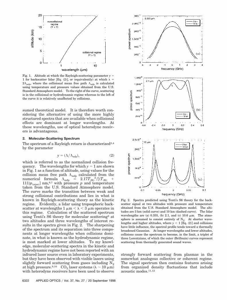
which is referred to as the normalized collision fre-quency. The wavelengths for which y 5 1 are shownn Fig. 1 as a function of altitude, using values for theollision mean free path Lmfp calculated from theumerical formula Lmfp 5 2.17T~K!

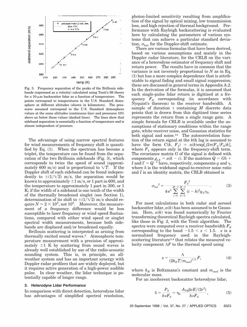
2y@~T~K! 1111!p~atm!# nm,6,7 with pressure p and temperaturetaken from the U.S. Standard Atmosphere model.The curve marks the transition between weak andstrong collisional contributions and lies in what isknown in Rayleigh-scattering theory as the kineticregime. Evidently, a lidar using tropospheric back-scatter at wavelengths 1 mm , l , 3 mm operates inhis regime. Calculation of the scattered spectrumsing Tenti’s S6 theory for molecular scattering8 at

two altitudes and three wavelengths of interest re-sults in the spectra given in Fig. 2. The sharpeningof the spectrum and its separation into three compo-nents at longer wavelengths when collisions domi-nate, in what is known as the hydrodynamic regime,is most marked at lower altitudes. To my knowl-edge, molecular-scattering spectra in the kinetic andhydrodynamic regime have not been reported with aninfrared laser source even in laboratory experiments,but they have been observed with visible lasers usingslightly forward scattering from gases including N2at high pressure.9,10 CO2 laser systems ~l ; 10 mm!

ith heterodyne receivers have been used to observe

Fig. 1. Altitude at which the Rayleigh-scattering parameter y 51 for backscatter lidar @Eq. ~2!#, or ~equivalently! at which l 52Lmfp, where the collisional mean free path Lmfp is calculatedusing temperature and pressure values obtained from the U.S.Standard Atmosphere model. To the right of the curve, scatteringis in the collisional or hydrodynamic regime whereas to the left ofthe curve it is relatively unaffected by collisions.

322 APPLIED OPTICS y Vol. 37, No. 27 y 20 September 1998

trongly forward scattering from plasmas in theomewhat analogous collective or coherent regime.he signal spectrum then contains features arising

rom organized density fluctuations that includecoustic modes.11,12

Fig. 2. Spectra predicted using Tenti’s S6 theory for the back-scatter signal at two altitudes with pressure and temperatureobtained from the U.S. Standard Atmosphere model. The alti-tudes are 3 km ~solid curve! and 10 km ~dashed curve!. The lidar

avelengths are ~a! 0.355, ~b! 2.1, and ~c! 10.6 mm. The atmo-phere is assumed to consist entirely of N2. At shorter wave-

lengths and higher altitudes, where y , 1 @Eq. ~2!# and collisionshave little influence, the spectral profile tends toward a thermallybroadened Gaussian. At longer wavelengths and lower altitudes,collisions cause the spectrum to become, in the limit, a triplet ofthree Lorentzians, of which the outer ~Brillouin! curves representscattering from thermally generated sound waves.

cm

k

pmaswDipt

Nsprssgb

fpssva

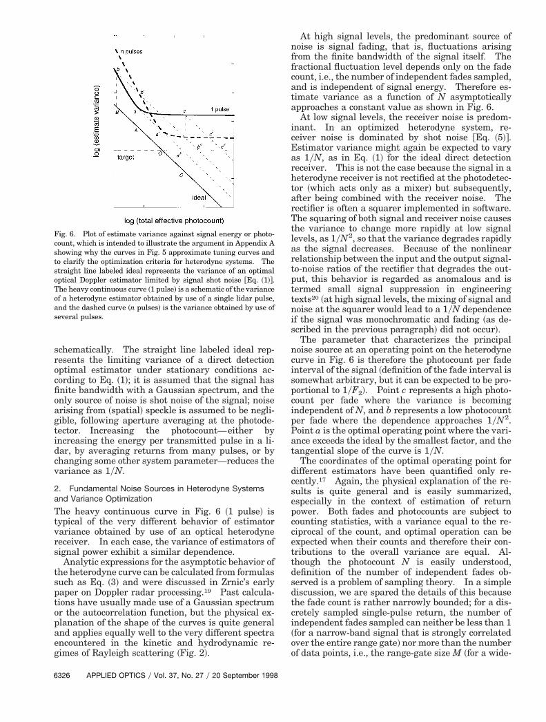
The advantage of using narrow spectral featuresfor wind measurements of frequency shift is quanti-fied by Eq. ~1!. When the spectrum has become atriplet, the temperature can be found from the sepa-ration of the two Brillouin sidebands ~Fig. 3!, whichorresponds to twice the speed of sound ~approxi-ately 600 mys! and is proportional to =T. If the

Doppler shift of each sideband can be found indepen-dently to 6~1y=2! mys, the separation would be

nown to approximately 61 mys, or 1 part in 600, andthe temperature to approximately 1 part in 300, or 1K; if the width of a sideband is one tenth of the widthof the thermally broadened singlet ~see Section 1!,determination of its shift to 6~1y=2! mys should re-quire N ' 2 3 103, not 105. Moreover, the measure-ment of a frequency difference would be lesssusceptible to laser frequency or wind speed fluctua-tions, compared with either wind speed or singletspectral width measurements, because both side-bands are displaced andyor broadened equally.

Brillouin scattering is interpreted as arising fromthermally excited sound waves.3 Atmospheric tem-

erature measurement with a precision of approxi-ately 61 K by scattering from sound waves is

lready well established by use of the radio-acousticounding system. This is, in principle, an all-eather system and has an important synergy withoppler radar profilers that are widely deployed, but

t requires active generation of a high-power audibleulse. In clear weather, the lidar technique is po-entially capable of longer range.

3. Heterodyne Lidar Performance

In comparison with direct detection, heterodyne lidarhas advantages of simplified spectral resolution,

20

photon-limited sensitivity resulting from amplifica-tion of the signal by optical mixing, low transmissionloss, and high rejection of thermal background. Per-formance with Rayleigh backscattering is evaluatedhere by calculating the parameters of various sys-tems that can achieve a particular standard devia-tion, shet for the Doppler-shift estimate.

There are various formulas that have been derived,based on various assumptions and mainly in theDoppler radar literature, for the CRLB on the vari-ance of a heterodyne estimator of frequency shift andreturn power. The results have in common that thevariance is not inversely proportional to N as in Eq.~1! but has a more complex dependence that is attrib-utable to signal fading and small signal suppression;these are discussed in general terms in Appendix A.2.In the derivation of the formulas, it is assumed thateach single-pulse lidar return is digitized at a fre-quency FS corresponding ~in accordance with

yquist’s theorem! to the receiver bandwidth. Aample of duration t containing M discrete dataoints that is drawn from this digitized time seriesepresents the return from a single range gate. Aimple formula for CRLB is available under the as-umptions of stationary conditions within the rangeate, white receiver noise, and Gaussian statistics foroth signal and noise.13 The autocorrelation func-

tion of the return signal at the kth lag is assumed tohave the form C~k, F1! 5 a~k!exp@ j2p~F1yFS!k#,where F1 appears only in the frequency-shift term.The covariance matrix G of the signal is defined withcomponents gi,k 5 a~k 2 i!. If the matrices Q 5 Gd 1I and G 5 Q21 have, respectively, components q and g,where d is the wideband signal-to-receiver noise ratioand I is an identity matrix, the CRLB obtained is

shet2 5

FS2

4p2 (i50

M21

(k50

M21

~i 2 k!2qikgki

. (3)

For most calculations in both radar and aerosolbackscatter lidar, a~k! has been assumed to be Gauss-ian. Here, a~k! was found numerically by Fouriertransforming theoretical Rayleigh spectra calculated,like those in Fig. 2, with the Tenti algorithm. Thespectra were computed over a receiver bandwidth FScorresponding to the band 21.5 , x , 1.5. x is anormalized frequency used in the Rayleigh-scattering literature3,4 that relates the measured ve-locity component LF to the thermal speed using

x 5L

~2kB Tymmol!1y2 F, (4)

where kB is Boltzmann’s constant and mmol is themolecular mass.

For an incoherent backscatter heterodyne lidar,

d 5PS

hnFS5 hL

ATRbcEy~2r2!

hnFS, (5)

Fig. 3. Frequency separation of the peaks of the Brillouin side-bands ~expressed as a velocity! calculated using Tenti’s S6 theoryor a 10-mm backscatter lidar as a function of temperature. Theoints correspond to temperatures in the U.S. Standard Atmo-phere at different altitudes ~shown in kilometers!. The pres-ures assumed correspond to the U.S. Standard Atmospherealues at the same altitudes ~continuous line! and pressures 10%bove an below these values ~dashed lines!. The lines show that

sideband separation is essentially a function of temperature and isalmost independent of pressure.

September 1998 y Vol. 37, No. 27 y APPLIED OPTICS 6323

tfilfrpb

l

tocww

1

Table 1. Parameters of the Three Heterodyne Lidarsa

6

where PS is the detected signal power calculated by alidar equation in which ATR is the area of a ~common!ransmit–receive antenna, b is the backscatter coef-cient, E the laser-pulse energy, c is the velocity of

ight, and r is the range. The lidar is assumed to beocused at each range to maximize the heterodyneeturn so that the results are not always those ex-ected of a lidar operating with a collimated outputeam. The overall lidar efficiency hL ~assumed here

to be 4%! is intended to take account of all systemlosses including photodetector quantum efficiency,antenna efficiency, excess receiver noise, and atmo-spheric transmission loss. The Rayleigh backscat-ter coefficient was calculated with b 5 1.39 @0.55y

~mm!#4 3 1026 m21 sr21 for sea level,15 corrected for

the altitude dependence of pressure.Table 1 lists the parameters of notional lidars op-

erating from the ground at three wavelengths usinglaser-pulse energies that are within the current stateof the art. I assumed that the losses in each systemare the same, and I adjusted ATR so that each systemgives approximately the same values in Fig. 4 for thepulse count needed to achieve shet 5 1 mys. It ap-pears that measurements to a precision of 61 myscould be obtained using any of the systems with ap-proximately 1000 pulses, or within 100 s at 10 Hz, ataltitudes as high as approximately 7 km with a 1-kmgate or as high as 5 km with a 100-m gate. No


explicit account is taken of the effects of wind ortemperature shear within the range gate or of refrac-tive turbulence.

The signal energy needed to make these measure-ments over n pulses, expressed as an effective accu-mulated photocount, N 5 nFStd 5 nMd, is shown inFig. 5. This plot confirms the lower photocountneeded at 10 mm, and to a lesser extent at 2 mm, as aresult of the more highly structured return spectrum.Comparing the two extreme wavelengths, approxi-mately 40–50 times as many photocounts are neededat 0.355 mm as at 10 mm. The results for 10 mm maybe conservative because the width of each of the threespectral peaks is a factor of over 10 less than the~Gaussian! spectrum at 0.355 mm, which should re-sult in a reduction of over 100 in the photocount @Eq.~1!#. In practice, greater advantage could be takenof spectral narrowing by filtering and processing thethree spectral features separately, discarding the in-termediate regions of the spectrum where the signalis low @Fig. 2~c!#.

The wavelength dependence of Rayleigh scatteringentails that the longer-wavelength systems requireincreased mean power and that their optics have tobe larger. Thus the product of pulse energy andoptics area needed for the 10-mm system ~from Table1, 1 J 3 0.287 m2! is approximately 640 times greaterthan that needed for the 0.355-mm system. How-ever, this is less than the factor ~10.6y0.355!3 '26,600 expected from the wavelength dependence ofthe Rayleigh photocount, again by the factor of ap-proximately 40. At a pulse repetition frequency of10 Hz, the mean transmitted power of each system isin the range 1–10 W, which is comparable with thatof some direct detection Rayleigh systems.6,16 Thetelescope apertures assumed here are also compara-ble with the direct detection systems, which havediameters between 0.3 and 1.3 m, although higher

Fig. 4. Number of lidar pulses n needed under stationary condi-ions to secure a standard deviation in the Doppler-shift estimatef 1 mys by use of a ground-based heterodyne lidar. For the solidurve plots, the lidar parameters are those listed in Table 1. Theavelengths are 0.355 mm ~x’s!, 2 mm ~filled squares!, and 10.6 mmith an output energy of 1 J ~open squares!. The dashed curve

corresponds to the same 10.6-mm system with an output energyincreased to 30 J; similar improvement could be obtained by in-creasing the throughput of the other systems by 30 times. In eachcase the range gate is 1 km ~for a 100-m gate the required pulsecount increases by a factor of approximately 10!.

Fig. 5. Effective photocount needed to obtain the results of Fig. 4,showing that ~i! the photocount needed to make a measurement isreduced by using lidar wavelengths in the collisional regime ~y .! where the spectra are more highly structured; and ~ii! for the

infrared systems, the minima that indicate that the proposed lidarparameters encompass the optimal operating point for a hetero-dyne system ~see Appendix A!. The symbols represent the samelidar parameters as in Fig. 4.

Wavelength, l ~mm! 0.355 2.1 10.6Laser-pulse energy, E ~J! 0.1 0.5 1Transceiver diameter ~m! 0.075 0.3 0.6

aAssumed for calculating the results shown with solid curves inFigs. 4 and 5.

Amb

pccfscecpS

atmtmab

optical quality is needed for the diffraction-limitedperformance required by a heterodyne lidar.

The data of Fig. 5 can be regarded as approxima-tions to heterodyne estimator tuning curves17 ~see

ppendix A.3!. The minima indicate the optimalatch between the return photocount and the num-

er of independent fades sampled.17 They also indi-cate the closest approach of the heterodyne CRLB tothe ideal and also therefore to the optimal resultobtainable from any direct detection system with thesame lidar system parameters and overall efficiencyhL ~see Appendix A.2. and A.3!. It is clear that theinfrared systems with returns from above 2 km andthe ultraviolet systems with returns from above 1 kmoperate in the small photocount per fade regime ~Ap-

endix A.2!. It is therefore difficult to foresee spa-eborne applications for the technique because of theonsiderable reduction in signal that would resultrom the much longer range. For comparativelyhort-range ground-based systems, however, signifi-ant improvement can be obtained by relatively mod-st increases in the lidar throughput. The fourthurve in Figs. 4 and 5 is constructed by use of thearameters of the large 10-mm lidar at the Mauipace Surveillance Site,18 which happen to be the

same as those given for the 10-mm system in Table 1,except that the laser-pulse energy is increased from 1to 30 J. This causes the projected standard devia-tion of a single-pulse measurement from 10 km to bereduced by a factor of approximately 30 and the num-ber of pulses required to achieve shet ; 1 mys to bereduced by a factor of approximately ~30!2 ' 1000; ata repetition rate of 10 Hz, this appears to permitDoppler wind and temperature measurements toabove 10 km within 10 s. This improvement, by afactor ;N2 rather than ;N, is a consequence of thedependence of shet on N rather than =N in the limitof low photocount per fade, which is discussed qual-itatively in Appendices A.2 and A.3.

4. Conclusions

Although the possibility of using infrared heterodynelidars to observe Rayleigh backscatter is perhaps sur-prising in view of the 1yl4 dependence, systems thatare suitable for preliminary studies already exist.Because the spectrum at 10 mm lies in the hydrody-namic regime and is strongly structured, the signalrequirements are not as different from those at 2 mms might be expected. They enable 10-mm systemso be considered for Doppler-shift and temperatureeasurements. Use of the Brillouin sidebands for

emperature has the advantage of being a differenceeasurement ~see Section 2!. The factor by which

erosol backscatter exceeds Rayleigh ~which is possi-ly greater than 103 at low altitude! entails a risk

that the wings of the aerosol return spectrum, whichis typically broadened by the laser-pulse bandwidthand range gate truncation, will compete with theBrillouin sidebands. Prior high-pass filtering willminimize the aerosol signal but it is likely to contam-inate observation of the narrow central feature of theRayleigh spectrum in the hydrodynamic regime ~Fig.

20

2!. Contamination will be significantly less atshorter wavelengths because both the ratio ofRayleigh-to-aerosol scattering cross section and theratio of sound speed frequency shift to ~the likely!laser-pulse bandwidth are relatively larger.

A 0.355-mm heterodyne lidar has been includedhere largely as a reference with which both directdetection systems at the same wavelength and theinfrared heterodyne systems can be compared. Itsperformance and compactness appear impressive,but it operates in the y , 1 regime, and interpretationof its results will be subject to the same problems~mentioned in Section 1! as direct detection systemsat this wavelength. Moreover, considerations in-cluding the wide receiver bandwidth, the tighter tol-erances needed to align diffraction-limited optics atshort wavelengths, beam attenuation resulting frommolecular scattering, vulnerability to refractive tur-bulence and multiple scattering, and the availabilityof suitable pulsed-transmitter and continuous localoscillator lasers, might make a heterodyne systemimpractical in this application.

The performance of the 2-mm system is, of course,intermediate between that of the other two. Suit-able lidars, with the parameters given in Table 1, arealready available, and development of more powerfullasers is ongoing. This wavelength is of interest be-cause the scattering is in the kinetic regime wherey ' 1 ~Fig. 1!. The spectral profile is then sensitiveto atmospheric parameters. This regime is optimalwhen determining molecular density from the spec-tral profile.1

The principal advantages of using heterodyne lidararise from the ability to resolve the spectra and sep-arate aerosol and molecular returns electronicallywithout interference from background light and thelikelihood that improved measurement precision canarise from the more structured spectra available inthe hydrodynamic regime. I have tried to show thatmeasurements could be attempted with existing sys-tems and that the approach has interesting potential.In principle, it is capable of temporally well-resolved ground-based or airborne measurements ofwind speed, temperature, and possibly pressure atlidar power levels that are comparable with thoseconsidered for both visible and ultraviolet direct de-tection systems and of substantially improved perfor-mance at slightly greater power levels.

Appendix A

Because observation of molecular scattering is usu-ally considered by use of direct detection systems,here I intend to summarize the optimization criteriafor optical heterodyne lidar receivers and, in partic-ular, to show why the curves in Fig. 5 approximatewhat have been called tuning curves.

1. Parametric Dependence of the Direct DetectionSystem Variance

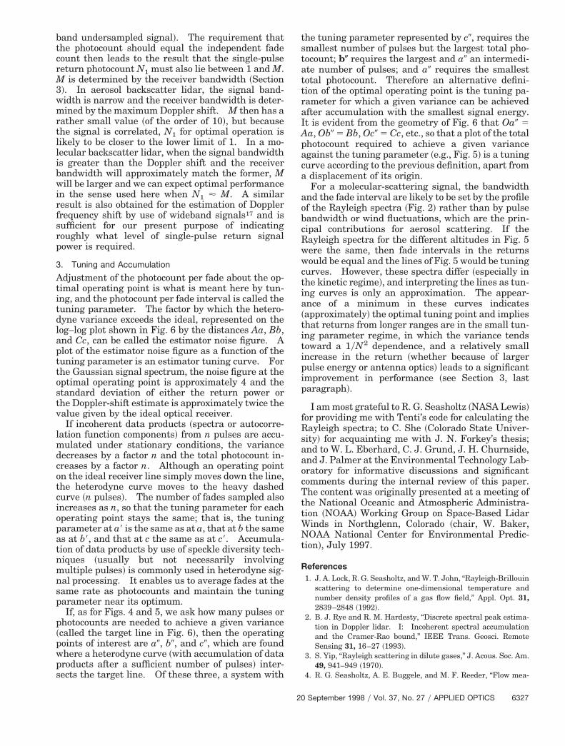
In Fig. 6, the dependence on signal energy ~or photo-count N! of the variance of estimators of Doppler-shiftfrequency by use of an optical system is depicted


topaeg

EarhtarTtl

sp

p

at

dc

dsdtci~oo

6

schematically. The straight line labeled ideal rep-resents the limiting variance of a direct detectionoptimal estimator under stationary conditions ac-cording to Eq. ~1!; it is assumed that the signal hasfinite bandwidth with a Gaussian spectrum, and theonly source of noise is shot noise of the signal; noisearising from ~spatial! speckle is assumed to be negli-gible, following aperture averaging at the photode-tector. Increasing the photocount—either byincreasing the energy per transmitted pulse in a li-dar, by averaging returns from many pulses, or bychanging some other system parameter—reduces thevariance as 1yN.

2. Fundamental Noise Sources in Heterodyne Systemsand Variance Optimization

The heavy continuous curve in Fig. 6 ~1 pulse! istypical of the very different behavior of estimatorvariance obtained by use of an optical heterodynereceiver. In each case, the variance of estimators ofsignal power exhibit a similar dependence.

Analytic expressions for the asymptotic behavior ofthe heterodyne curve can be calculated from formulassuch as Eq. ~3! and were discussed in Zrnic’s earlypaper on Doppler radar processing.19 Past calcula-ions have usually made use of a Gaussian spectrumr the autocorrelation function, but the physical ex-lanation of the shape of the curves is quite generalnd applies equally well to the very different spectrancountered in the kinetic and hydrodynamic re-imes of Rayleigh scattering ~Fig. 2!.


At high signal levels, the predominant source ofnoise is signal fading, that is, fluctuations arisingfrom the finite bandwidth of the signal itself. Thefractional fluctuation level depends only on the fadecount, i.e., the number of independent fades sampled,and is independent of signal energy. Therefore es-timate variance as a function of N asymptoticallyapproaches a constant value as shown in Fig. 6.

At low signal levels, the receiver noise is predom-inant. In an optimized heterodyne system, re-ceiver noise is dominated by shot noise @Eq. ~5!#.

stimator variance might again be expected to varys 1yN, as in Eq. ~1! for the ideal direct detectioneceiver. This is not the case because the signal in aeterodyne receiver is not rectified at the photodetec-or ~which acts only as a mixer! but subsequently,fter being combined with the receiver noise. Theectifier is often a squarer implemented in software.he squaring of both signal and receiver noise causeshe variance to change more rapidly at low signalevels, as 1yN2, so that the variance degrades rapidly

as the signal decreases. Because of the nonlinearrelationship between the input and the output signal-to-noise ratios of the rectifier that degrades the out-put, this behavior is regarded as anomalous and istermed small signal suppression in engineeringtexts20 ~at high signal levels, the mixing of signal andnoise at the squarer would lead to a 1yN dependenceif the signal was monochromatic and fading ~as de-scribed in the previous paragraph! did not occur!.

The parameter that characterizes the principalnoise source at an operating point on the heterodynecurve in Fig. 6 is therefore the photocount per fadeinterval of the signal ~definition of the fade interval isomewhat arbitrary, but it can be expected to be pro-ortional to 1yF2!. Point c represents a high photo-

count per fade where the variance is becomingindependent of N, and b represents a low photocount

er fade where the dependence approaches 1yN2.Point a is the optimal operating point where the vari-nce exceeds the ideal by the smallest factor, and theangential slope of the curve is 1yN.

The coordinates of the optimal operating point forifferent estimators have been quantified only re-ently.17 Again, the physical explanation of the re-

sults is quite general and is easily summarized,especially in the context of estimation of returnpower. Both fades and photocounts are subject tocounting statistics, with a variance equal to the re-ciprocal of the count, and optimal operation can beexpected when their counts and therefore their con-tributions to the overall variance are equal. Al-though the photocount N is easily understood,

efinition of the number of independent fades ob-erved is a problem of sampling theory. In a simpleiscussion, we are spared the details of this becausehe fade count is rather narrowly bounded; for a dis-retely sampled single-pulse return, the number ofndependent fades sampled can neither be less than 1for a narrow-band signal that is strongly correlatedver the entire range gate! nor more than the numberf data points, i.e., the range-gate size M ~for a wide-

Fig. 6. Plot of estimate variance against signal energy or photo-count, which is intended to illustrate the argument in Appendix Ashowing why the curves in Fig. 5 approximate tuning curves andto clarify the optimization criteria for heterodyne systems. Thestraight line labeled ideal represents the variance of an optimaloptical Doppler estimator limited by signal shot noise @Eq. ~1!#.The heavy continuous curve ~1 pulse! is a schematic of the varianceof a heterodyne estimator obtained by use of a single lidar pulse,and the dashed curve ~n pulses! is the variance obtained by use ofseveral pulses.

tcrM3wmrt

WNt

band undersampled signal!. The requirement thathe photocount should equal the independent fadeount then leads to the result that the single-pulseeturn photocount N1 must also lie between 1 and M.

is determined by the receiver bandwidth ~Section!. In aerosol backscatter lidar, the signal band-idth is narrow and the receiver bandwidth is deter-ined by the maximum Doppler shift. M then has a

ather small value ~of the order of 10!, but becausehe signal is correlated, N1 for optimal operation is

likely to be closer to the lower limit of 1. In a mo-lecular backscatter lidar, when the signal bandwidthis greater than the Doppler shift and the receiverbandwidth will approximately match the former, Mwill be larger and we can expect optimal performancein the sense used here when N1 ' M. A similarresult is also obtained for the estimation of Dopplerfrequency shift by use of wideband signals17 and issufficient for our present purpose of indicatingroughly what level of single-pulse return signalpower is required.

3. Tuning and Accumulation

Adjustment of the photocount per fade about the op-timal operating point is what is meant here by tun-ing, and the photocount per fade interval is called thetuning parameter. The factor by which the hetero-dyne variance exceeds the ideal, represented on thelog–log plot shown in Fig. 6 by the distances Aa, Bb,and Cc, can be called the estimator noise figure. Aplot of the estimator noise figure as a function of thetuning parameter is an estimator tuning curve. Forthe Gaussian signal spectrum, the noise figure at theoptimal operating point is approximately 4 and thestandard deviation of either the return power orthe Doppler-shift estimate is approximately twice thevalue given by the ideal optical receiver.

If incoherent data products ~spectra or autocorre-lation function components! from n pulses are accu-mulated under stationary conditions, the variancedecreases by a factor n and the total photocount in-creases by a factor n. Although an operating pointon the ideal receiver line simply moves down the line,the heterodyne curve moves to the heavy dashedcurve ~n pulses!. The number of fades sampled alsoincreases as n, so that the tuning parameter for eachoperating point stays the same; that is, the tuningparameter at a9 is the same as at a, that at b the sameas at b9, and that at c the same as at c9. Accumula-tion of data products by use of speckle diversity tech-niques ~usually but not necessarily involvingmultiple pulses! is commonly used in heterodyne sig-nal processing. It enables us to average fades at thesame rate as photocounts and maintain the tuningparameter near its optimum.

If, as for Figs. 4 and 5, we ask how many pulses orphotocounts are needed to achieve a given variance~called the target line in Fig. 6!, then the operatingpoints of interest are a0, b0, and c0, which are foundwhere a heterodyne curve ~with accumulation of dataproducts after a sufficient number of pulses! inter-sects the target line. Of these three, a system with

20

the tuning parameter represented by c0, requires thesmallest number of pulses but the largest total pho-tocount; b( requires the largest and a0 an intermedi-ate number of pulses; and a0 requires the smallesttotal photocount. Therefore an alternative defini-tion of the optimal operating point is the tuning pa-rameter for which a given variance can be achievedafter accumulation with the smallest signal energy.It is evident from the geometry of Fig. 6 that Oa0 5Aa, Ob0 5 Bb, Oc0 5 Cc, etc., so that a plot of the totalphotocount required to achieve a given varianceagainst the tuning parameter ~e.g., Fig. 5! is a tuningcurve according to the previous definition, apart froma displacement of its origin.

For a molecular-scattering signal, the bandwidthand the fade interval are likely to be set by the profileof the Rayleigh spectra ~Fig. 2! rather than by pulsebandwidth or wind fluctuations, which are the prin-cipal contributions for aerosol scattering. If theRayleigh spectra for the different altitudes in Fig. 5were the same, then fade intervals in the returnswould be equal and the lines of Fig. 5 would be tuningcurves. However, these spectra differ ~especially inthe kinetic regime!, and interpreting the lines as tun-ing curves is only an approximation. The appear-ance of a minimum in these curves indicates~approximately! the optimal tuning point and impliesthat returns from longer ranges are in the small tun-ing parameter regime, in which the variance tendstoward a 1yN2 dependence, and a relatively smallincrease in the return ~whether because of largerpulse energy or antenna optics! leads to a significantimprovement in performance ~see Section 3, lastparagraph!.

I am most grateful to R. G. Seasholtz ~NASA Lewis!for providing me with Tenti’s code for calculating theRayleigh spectra; to C. She ~Colorado State Univer-sity! for acquainting me with J. N. Forkey’s thesis;and to W. L. Eberhard, C. J. Grund, J. H. Churnside,and J. Palmer at the Environmental Technology Lab-oratory for informative discussions and significantcomments during the internal review of this paper.The content was originally presented at a meeting ofthe National Oceanic and Atmospheric Administra-tion ~NOAA! Working Group on Space-Based Lidar

inds in Northglenn, Colorado ~chair, W. Baker,OAA National Center for Environmental Predic-

ion!, July 1997.

References1. J. A. Lock, R. G. Seasholtz, and W. T. John, “Rayleigh-Brillouin

scattering to determine one-dimensional temperature andnumber density profiles of a gas flow field,” Appl. Opt. 31,2839–2848 ~1992!.

2. B. J. Rye and R. M. Hardesty, “Discrete spectral peak estima-tion in Doppler lidar. I: Incoherent spectral accumulationand the Cramer-Rao bound,” IEEE Trans. Geosci. RemoteSensing 31, 16–27 ~1993!.

3. S. Yip, “Rayleigh scattering in dilute gases,” J. Acous. Soc. Am.49, 941–949 ~1970!.

4. R. G. Seasholtz, A. E. Buggele, and M. F. Reeder, “Flow mea-


surements based on Rayleigh scattering and Fabry-Perot in-

1

cesses and applications to radar processing of atmospheric

1

1

1

1

1

1

2

6

terferometer,” Opt. Lasers 27, 543–570 ~1997!.5. A. T. Young and G. W. Kattawar, “Rayleigh scattering line

profiles,” Appl. Opt. 22, 3668–3670 ~1983!.6. H. Shimizu, S. A. Lee, and C. Y. She, “High spectral resolution

lidar system with atomic blocking filters for measuring atmo-spheric parameters,” Appl. Opt. 22, 1373–1381 ~1983!.

7. J. N. Forkey, “Development and demonstration of filtered Ray-leigh scattering: a laser-based flow diagnostic for planarmeasurement of velocity,” Ph.D. dissertation ~Princeton Uni-versity, Princeton N.J., 1996!.

8. G. Tenti, C. D. Boley, and R. C. Desai, “On the kinetic modeldescription of Rayleigh-Brillouin scattering from moleculargases,” Can. J. Phys. 52, 285–290 ~1974!.

9. R. P. Sandoval and R. L. Armstrong, “Rayleigh-Brillouin scat-tering in molecular nitrogen,” Phys. Rev. A 13, 752–757 ~1976!.

10. Q. H. Lao, P. E. Schoen, and B. Chu, “Rayleigh-Brillouin scat-tering of gases with internal relaxation,” J. Chem. Phys. 64,3547–3554 ~1976!.

11. E. Holzhauer, “Forward scattering at 10.6 mm using light mix-ing to measure the ion temperature in a hydrogen arc plasma,”Phys. Lett. A 62, 495–497 ~1997!.

12. R. E. Slusher and C. M. Surko, “Study of density fluctuationsin plasmas by small-angle CO2 laser scattering,” Phys. Fluids23, 472–490 ~1980!.

3. R. G. Frehlich, “Cramer-Rao bound for Gaussian random pro-


signals,” IEEE Trans. Geosci. Remote Sensing 31, 1123–1131~1993!.

4. B. J. Rye, “The reference range for atmospheric backscatterlidar,” Opt. Quantum Electron. 11, 441–446 ~1979!.

5. R. T. H. Collins and P. B. Russell, “Lidar measurement ofparticles and gases by elastic backscattering and differentialabsorption,” in Laser Monitoring of the Atmosphere, E. D. Hin-kley, ed., Vol. 14 of Topics in Applied Physics, ~Springer-Verlag, Berlin, 1976!.

6. M. L. Chanin, A. Garnier, A. Hauchecorne, and J. Porteneuve,“A Doppler lidar for measuring winds in the middle atmo-sphere,” Geophys. Res. Lett. 16, 1273–1276 ~1989!.

7. B. J. Rye and R. M. Hardesty, “Estimate optimization param-eters for incoherent backscatter heterodyne lidar,” Appl. Opt.36, 9425–9436 ~1997!; errata, 37, 4016 ~1998!.

8. V. Hasson and F. Corbett, “Long-range coherent frequencyagile laser radars for precision tracking, imaging, and chemi-cal detection applications,” in Proceedings of the Ninth Confer-ence on Coherent Laser Radar ~Swedish Defence ResearchEstablishment, Linkoping, Sweden, 1997!, p. W1.

9. D. S. Zrnic, “Estimation of spectral moments for weather ech-oes,” IEEE Trans. Geosci. Electron. GE-17, 113–128 ~1979!.

0. W. B. Davenport and W. T. Root, Random Signals and Noise~McGraw-Hill, New York, 1958!.

Download - Molecular Backscatter Heterodyne Lidar: A Computational Evaluation

Top Related