Download - Methodological proposal for predictive and cartographic ... · Methodological proposal for predictive and cartographic modeling of insect population: Semidalis kolbei case, the Araucanía

crop protection

Cien. Inv. Agr. 38(3):379-390. 2011www.rcia.uc.cl

research paper

Methodological proposal for predictive and cartographic modeling of insect population: Semidalis kolbei case, the Araucanía Region, Chile

Nelson Ojeda1, Ramón Rebolledo2, Soraya Calzadilla1, Hector Soto1, and Luis Morales3

1Departamento de Ciencias Forestales, Facultad de Ciencias Agropecuarias y Forestales, Universidad de la Frontera. Casilla 54-D. Temuco. Chile.

2Departamento de Ciencias Agronómicas y Recursos Naturales, Facultad de Ciencias Agropecuarias y Forestales, Universidad de la Frontera. Casilla 54-D. Temuco. Chile.

3Departamento de Ciencias Ambientales y Recursos Naturales Renovables, Facultad de Ciencias Agronómicas, Universidad de Chile. Casilla 1004. Santiago. Chile.

Abstract

N. Ojeda, R. Rebolledo, S. Calzadilla, H. Soto, and L. Morales. 2011. Methodological proposal for predictive and cartographic modeling of insect population: Semidalis kolbei case, the Araucanía Region, Chile. Cien. Inv. Agr. 38(3): 379-390. Semidalis kolbei occupies a significant area of south central Chile. However, it is necessary to determine and predict the occurrence of the insect at a given site. The aim of this research is to analyze the potential spatial distribution of S. kolbei in La Araucanía Region of Chile. The study compares ordinary kriging (OK) interpolation methods, geographically weighted regression (GWR) and global regression (GR). The following variables were used in the investigation: topography (altitude, aspect, and slope), distance from the littoral, climate, and geographical variables (latitude and longitude). Of the models evaluated, the GWR proved to be the most successful. This model revealed a marked east-west gradient in the distribution of S. kolbei and a relationship with altitude.

Key words: Araucanía Region, Chile, modeling, potential spatial distribution, Semidalis kolbei.

Introduction

Semidalis kolbei Enderlein is economically important because of its predatory behavior on agricultural pests. In addition, it has a broad spatial distribution (SD) and can adapt to different plant formations. Therefore, it is an excellent agent for biological control (Prado, 1991; Rebolledo et al., 2009).

However, research in Chile based on collections and field data has traditionally lacked information on orders, families, and species needed to construct maps. Therefore, this study is important because the potential spatial distribution (PSD) of an insect is modeled from field data to generate predictions. Previous biogeographic studies of biological control agents conducted in Chile have focused on the description of the diversity of the order Coleoptera in the Bíobío Region (Vergara et al., 2006) with-out using predictive models, as previously stated. However, Jerez (2000) studied the biogeography of

Recieved January 12, 2010. Accepted September 27, 2011.Corresponding author: [email protected]

ciencia e investigación agraria380

the Coleoptera in desert ecosystems in the Region of Antofagasta. The results of this study indicated that most of the species breed at altitudes greater than 2,000 masl. Propose that the consideration of altitudinal variation is important in studies on distribution. The methodology used in the current study is original because the study is the first work conducted in Chile to predict the PSD of a species using geospatial modeling. However, Valverde-Jiménez et al. (2007) justify the study of only one insect species and concede that studies on higher taxa (i.e., families or orders) are equally important because they indicate distributional trends. Therefore, this research is especially valu-able because S. kolbei is inconspicuous and small (3 to 7 mm in length).

The compilation of biological information requires collections, the development of a compendium and cartographic modeling. This information is needed to counteract environmental deterioration and provides the basis for species conservation programs (Wilson, 1988; Murphy, 1990; Lobo and Martín-Piera, 1991; Davis, 1994; Margules and Austin, 1994; Jiménez-Valverde and Lobo, 2007; Lobo et al., 2007). In this context, reasonable predictions of the SD of a species are possible through the use of indicator variables and information about the environment. Thus, a number of criteria are suggested for select-ing these variables. In addition, use is made of those variables that offer a better representation of the local

conditions of the region, e.g., topographic variables (Ter Braak and Looman, 1995; Wohlgemuth, 1998).

The aim of this research is to analyze the potential spatial distribution of individuals of S. kolbei in La Araucanía Region using ordinary kriging (OK), geographically weighted regressions (GWR) and global regression (GR) as interpolation methods.

Materials and methods

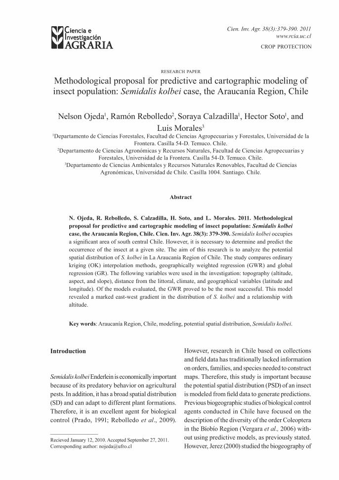
The study area was the Araucanía Region (Figure 1). The Universal Transversal Mercator (UTM) projection and World Geodetic System datum 84 (WGS84) specify the location of the area in met-ric units as XMin, YMin: 628940, 5607600 and XMax, YMax: 863260, 5838690. For this study in La Araucanía Region, zone H has been mapped to time zone 18 and zone 18 extended. Therefore, the fieldwork and the spatial representation of the species were averaged to avoid problems with corrections and transformations (Borgel, 1983; Raisz, 1985; Valdés, 1989; Ruiz, 1998). The topographic model used in this study has been developed using the NASA database (2004). The application of Geographical Information Systems (GIS) allowed the systematization of the biological information for further cartographic use. Based on this information, the spatial distribution of S. kolbei was related to the physical environment.

Figure 1. Sample locations (yellow triangles) (with geographical coordinates in latitude and longitude) of Semidalis kolbei in La Araucanía Region, Chile. Grid 25 x 25 km. A superimposed digital elevation model is also shown.

381VOLUME 38 Nº3 SEPTEMBER – DECEMBER 2011

The entomological sampling performed in the field was georeferenced using the five agroeco-logical zones described by Rouanet et al. (1988) and the vegetation cartography presented by Gajardo (1994) as criteria. This approach covered most of the region. A minimum of six to eight sampling stations per visit was established in each agroecological zone. Sweeps with insect nets were performed on all vegetation present at each station. All individuals observed in the field were counted and recorded. Samples were collected from September through May in 2005-2006, 2006-2007, 2007-2008 and 2008-2009. Published results based on collections by one of the authors of this work were used as data for the years corresponding to September through May of 2003-2004 and 2004-2005 (Rebolledo et al., 2009).

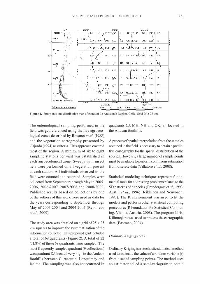
The study area was detailed on a grid of 25 x 25 km squares to improve the systematization of the information collected. This proposed grid included a total of 69 quadrants (Figure 2). A total of 22 (31.8%) of these 69 quadrants were sampled. The most frequently sampled quadrant (9 collections) was quadrant DJ, located very high in the Andean foothills between Curacautín, Lonquimay and Icalma. The sampling was also concentrated in

quadrants CJ, MH, NH and QK, all located in the Andean foothills.

A process of spatial interpolation from the samples obtained in the field is necessary to obtain a predic-tive cartography for the spatial distribution of the species. However, a large number of sample points must be available to perform continuous estimation from discrete data (Villatoro et al., 2008).

Statistical modeling techniques represent funda-mental tools for addressing problems related to the SD patterns of a species (Prendergast et al., 1993; Austin et al., 1996; Heikkinen and Neuvonen, 1997). The R environment was used to fit the models and perform other statistical computing procedures (R Foundation for Statistical Comput-ing. Vienna, Austria. 2008). The program Idrisi Kilimanjaro was used to process the cartographic data (Eastman, 2004).

Ordinary Kriging (OK)

Ordinary Kriging is a stochastic statistical method used to estimate the value of a random variable (z) from a set of sampling points. The method uses an estimator called a semi-variogram to obtain

Figure 2. Study area and distribution map of zones of La Araucanía Region, Chile. Grid 25 x 25 km.


this estimate by describing the spatial continuities in the sampling data (Webster and Oliver, 2007). The OK method estimates the values ẑ (u*) as a linear combination of the fluctuating means of the n observations, defined by:

( )*

1

ˆ( ) ( )n

i ii

z u u z uλ=

= ∑ (1)

where ẑ (u*) is the value estimated for u, z(ui) is the observed value and

11

n

ii

λ=

=∑ . The weights ( iλ ) cor-responding to each point are estimated from the solutions of a system of linear equations obtained by assuming that z(ui) is a sample derived from a random process. This method has also been used for interpolating climate data (Martinez-Cob, 1996; Miranda-Salas and Condal, 2003; Vicente-Serrano et al., 2003).

Global regression (GR)

This method is normally applied to large surfaces. The SD of a variable that depends on other vari-ables is defined by a unique equation. In a global analysis, the model is built from point values collected in the field using traditional sampling techniques. Therefore, the values estimated for sites without measurements are calculated with this unique relation. This method does not consider local effects (Fotheringam et al., 2000). The GR model is obtained from a function that includes geographic variables (latitude and longitude) and topographic variables (altitude, exposure, gradient, distance to the coastline). The equation that integrates these models is expressed by the following linear combination (Canessa, 2006; Morales et al., 2006; Díaz et al., 2010):

(2)

where F (x1, x2,...,xn ) is the dependent variable, aj are the coefficients to be determined, n

kx are the descriptor variables used and e is the error in the model.

The statistical problem addressed by the model is related to the concept of spatial heterogeneity (Anselin, 2000). This spatial effect occurs if a phenomenon represented by a numerical model changes its func-tional relationship with the parameters that define that phenomenon in space. Hence, the resulting effect on the functional relationship might be related directly to the geographic location of the area under study (Anselin, 1998; Chasco, 2003; Kamisnky and Radosz, 2003). As an effect resulting from heterogeneity, it resides primarily in the relevant geographic space. Accordingly, the localization of the sampling points or observations is fundamental for determining the functional structure of that vari-ability (Moreno and Vayá, 2000). A problem called parametric instability arises in connection with the model of spatial heterogeneity. The problem is related to the lack of stability of an environmental variable. This lack of stability corresponds to the intrinsic spatial variability of the variable. In this situation, the parameters of a regression vary ac-cording to the geographic location.

Geographically weighted regressions (GWR)

These regressions are useful for modeling the phenomenon of continuous parametric instability (Draper and Smith, 1981). Global regressions are used to describe the spatial behavior of an environ-mental variable with a unique equation. However, the coefficients of this equation vary spatially (Morales et al., 2007; Morales et al., 2010). The search for the coefficients corresponding to the best-fitting equation is made with the minimum weighted squares. The weights are related to a function that measures the distance between each point and the other points (Berry and Feldman, 1985; Fotheringham et al., 2002). Accordingly, the following general model is proposed:

^ ^

01

N

ii ii

y X eβ β=

= + ⋅ +∑ (3)

where ^

iβ is a vector of parameters obtained through minimum weighted squares as follows:


(4)[ ] 1' 'i i iX W X X W yβ∧ −= ⋅ ⋅ ⋅ ⋅

Wi is a diagonal matrix of order (N, N). The elements on the diagonal of this matrix are the weights wij that represent the values of the distance function specifying the distance between the observation considered and the other observations. The follow-ing structure for the function defining the weights is suggested as an example (Fotheringham et al., 1997) and calculated with the equation

(5)2ijd

ijw e α−=

where α is a parameter expressing the decrease between two points in the space and dij is the distance between the points i and j. Finally, e is the error of estimation. From a practical point of view, a point located farther from i will exert less statistical influence on the final numerical relation (Morales et al., 2007).

An linear regression of the estimated values (Y) on the observed values (X) was calculated to compare the data on the number of individu-als counted in the field with the data obtained from the proposed methods (Shannon, 1988). The parameters of the regression equation were evaluated using tests of simultaneous hypotheses for the intercept (Ho: a = 0) and the slope (Ho: b = 1). Student T-test with P £ 0.05 was used (Steel and Torrie, 1988). Additionally, the root mean square error of the prediction (RMSE) was calculated. The result was expressed in absolute units and as a percentage. The percentage was calculated in relation to the average value obtained from the observations. This coefficient indicates the degree of overestimation or underestima-tion by the model relative to the average of the observed values.

( )2

1 100( )Pr

n

i ii

ValEstim ValObsRMSE

n ValObs om=

−=

∑ (6)

In equation (6), ValEstimi and ValObsi represent the estimated values corresponding to the obser-

vations and the field observations, respectively. ValObsProm is the average of the observations, and n represents the number of data points used in the estimate.

Results

The sampling sites were distributed longitudinally from the Coastal Range (commune of Trovolhue) to the Andes mountain range (commune of Lon-quimay) (Figure 1). The most northern commune sampled was Angol, and the most southern was Curarrehue. The sampling was concentrated in the Andean foothills and the Andes Mountains, where 27 quadrants were sampled. A total of 35 quadrants were sampled between the Valley and the foothills of the Coastal Range. The sites sampled presented substantial differences in altitude. The highest locality was the commune of Lonquimay, 1657.3 masl, whereas the lowest was Trovolhue, 22.8 masl, The models used in this study included the topography because of this important difference in altitude.

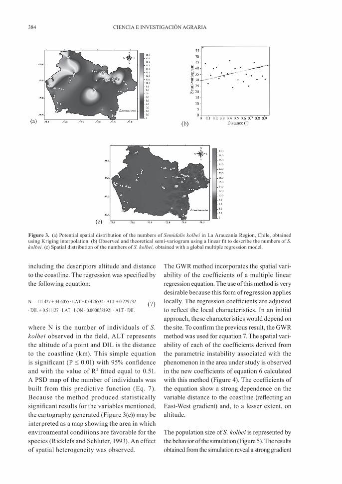
The results of the interpolation with the Kriging method are shown (Figure 3(a)) in combination with a linear variogram (Figure 3(b)). The sampling was concentrated in the Andes Mountain Range towards the Coastal Range; therefore, the results reflect a sampling bias (Figure 2). The image (Figure 3) presents the number of individuals of S. kolbei projected by the simulation. This method reveals a gradient in the numbers of S. kolbei in La Araucanía Region. The gradient is associated with the local effects of variation in altitude. An estimate of the number of individu-als of S. kolbei observed in the sampling areas was obtained from a stepwise multiple regres-sion model that included the spatial variables latitude, longitude, altitude and distance to the coastline (Figure 3(b)).

The global multiple regression (GR) expressed the relationship between the number of individuals and the geographic and topographic variables,


including the descriptors altitude and distance to the coastline. The regression was specified by the following equation:

(7)N = -111.427 + 34.6055 ∙ LAT + 0.0126534 ∙ ALT + 0.229732

∙ DIL + 0.511127 ∙ LAT ∙ LON - 0.0000581921 ∙ ALT ∙ DIL

where N is the number of individuals of S. kolbei observed in the field, ALT represents the altitude of a point and DIL is the distance to the coastline (km). This simple equation is significant (P ≤ 0.01) with 95% confidence and with the value of R2 fitted equal to 0.51. A PSD map of the number of individuals was built from this predictive function (Eq. 7). Because the method produced statistically significant results for the variables mentioned, the cartography generated (Figure 3(c)) may be interpreted as a map showing the area in which environmental conditions are favorable for the species (Ricklefs and Schluter, 1993). An effect of spatial heterogeneity was observed.

Figure 3. (a) Potential spatial distribution of the numbers of Semidalis kolbei in La Araucanía Region, Chile, obtained using Kriging interpolation. (b) Observed and theoretical semi-variogram using a linear fit to describe the numbers of S. kolbei. (c) Spatial distribution of the numbers of S. kolbei, obtained with a global multiple regression model.

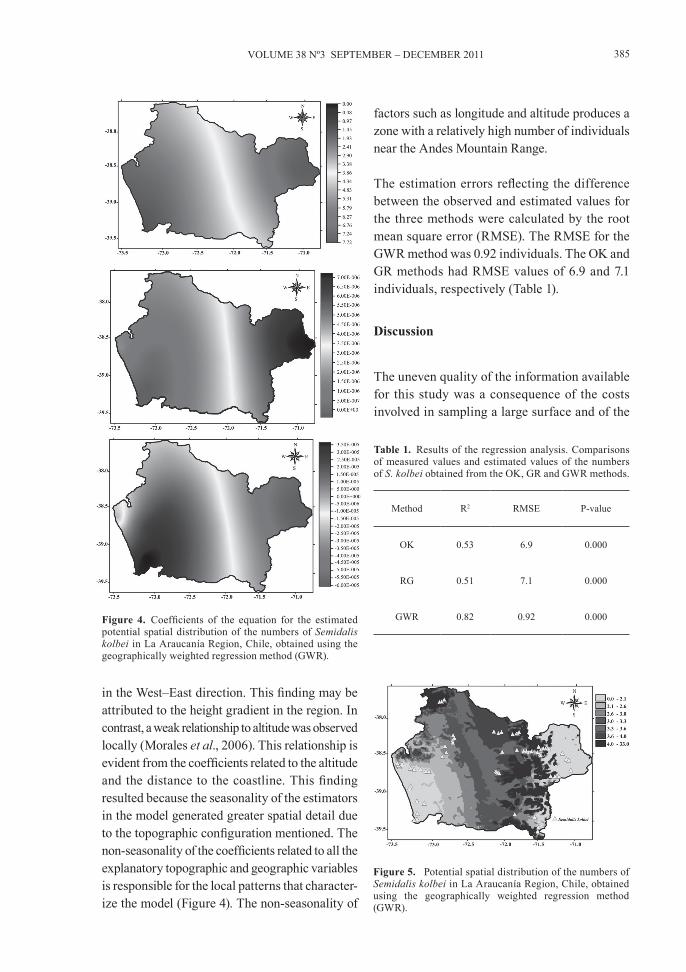
The GWR method incorporates the spatial vari-ability of the coefficients of a multiple linear regression equation. The use of this method is very desirable because this form of regression applies locally. The regression coefficients are adjusted to reflect the local characteristics. In an initial approach, these characteristics would depend on the site. To confirm the previous result, the GWR method was used for equation 7. The spatial vari-ability of each of the coefficients derived from the parametric instability associated with the phenomenon in the area under study is observed in the new coefficients of equation 6 calculated with this method (Figure 4). The coefficients of the equation show a strong dependence on the variable distance to the coastline (reflecting an East-West gradient) and, to a lesser extent, on altitude.

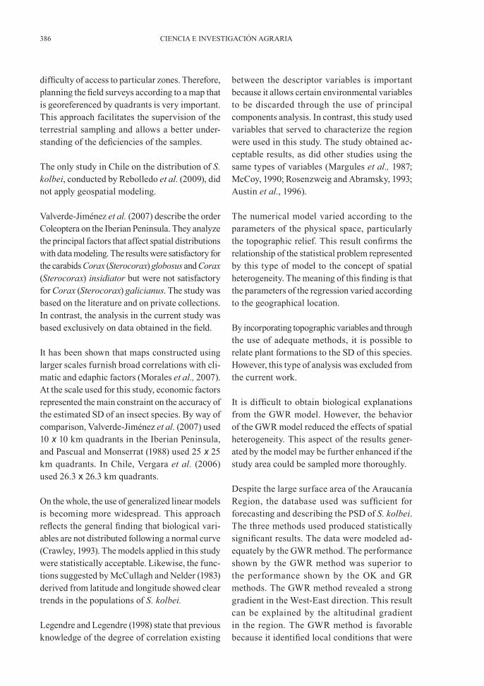
The population size of S. kolbei is represented by the behavior of the simulation (Figure 5). The results obtained from the simulation reveal a strong gradient


in the West–East direction. This finding may be attributed to the height gradient in the region. In contrast, a weak relationship to altitude was observed locally (Morales et al., 2006). This relationship is evident from the coefficients related to the altitude and the distance to the coastline. This finding resulted because the seasonality of the estimators in the model generated greater spatial detail due to the topographic configuration mentioned. The non-seasonality of the coefficients related to all the explanatory topographic and geographic variables is responsible for the local patterns that character-ize the model (Figure 4). The non-seasonality of

factors such as longitude and altitude produces a zone with a relatively high number of individuals near the Andes Mountain Range. The estimation errors reflecting the difference between the observed and estimated values for the three methods were calculated by the root mean square error (RMSE). The RMSE for the GWR method was 0.92 individuals. The OK and GR methods had RMSE values of 6.9 and 7.1 individuals, respectively (Table 1).

Discussion

The uneven quality of the information available for this study was a consequence of the costs involved in sampling a large surface and of the

Figure 4. Coefficients of the equation for the estimated potential spatial distribution of the numbers of Semidalis kolbei in La Araucanía Region, Chile, obtained using the geographically weighted regression method (GWR).

Figure 5. Potential spatial distribution of the numbers of Semidalis kolbei in La Araucanía Region, Chile, obtained using the geographically weighted regression method (GWR).

Table 1. Results of the regression analysis. Comparisons of measured values and estimated values of the numbers of S. kolbei obtained from the OK, GR and GWR methods.

Method R2 RMSE P-value

OK 0.53 6.9 0.000

RG 0.51 7.1 0.000

GWR 0.82 0.92 0.000


difficulty of access to particular zones. Therefore, planning the field surveys according to a map that is georeferenced by quadrants is very important. This approach facilitates the supervision of the terrestrial sampling and allows a better under-standing of the deficiencies of the samples.

The only study in Chile on the distribution of S. kolbei, conducted by Rebolledo et al. (2009), did not apply geospatial modeling.

Valverde-Jiménez et al. (2007) describe the order Coleoptera on the Iberian Peninsula. They analyze the principal factors that affect spatial distributions with data modeling. The results were satisfactory for the carabids Corax (Sterocorax) globosus and Corax (Sterocorax) insidiator but were not satisfactory for Corax (Sterocorax) galicianus. The study was based on the literature and on private collections. In contrast, the analysis in the current study was based exclusively on data obtained in the field.

It has been shown that maps constructed using larger scales furnish broad correlations with cli-matic and edaphic factors (Morales et al., 2007). At the scale used for this study, economic factors represented the main constraint on the accuracy of the estimated SD of an insect species. By way of comparison, Valverde-Jiménez et al. (2007) used 10 x 10 km quadrants in the Iberian Peninsula, and Pascual and Monserrat (1988) used 25 x 25 km quadrants. In Chile, Vergara et al. (2006) used 26.3 x 26.3 km quadrants.

On the whole, the use of generalized linear models is becoming more widespread. This approach reflects the general finding that biological vari-ables are not distributed following a normal curve (Crawley, 1993). The models applied in this study were statistically acceptable. Likewise, the func-tions suggested by McCullagh and Nelder (1983) derived from latitude and longitude showed clear trends in the populations of S. kolbei.

Legendre and Legendre (1998) state that previous knowledge of the degree of correlation existing

between the descriptor variables is important because it allows certain environmental variables to be discarded through the use of principal components analysis. In contrast, this study used variables that served to characterize the region were used in this study. The study obtained ac-ceptable results, as did other studies using the same types of variables (Margules et al., 1987; McCoy, 1990; Rosenzweig and Abramsky, 1993; Austin et al., 1996).

The numerical model varied according to the parameters of the physical space, particularly the topographic relief. This result confirms the relationship of the statistical problem represented by this type of model to the concept of spatial heterogeneity. The meaning of this finding is that the parameters of the regression varied according to the geographical location.

By incorporating topographic variables and through the use of adequate methods, it is possible to relate plant formations to the SD of this species. However, this type of analysis was excluded from the current work.

It is difficult to obtain biological explanations from the GWR model. However, the behavior of the GWR model reduced the effects of spatial heterogeneity. This aspect of the results gener-ated by the model may be further enhanced if the study area could be sampled more thoroughly.

Despite the large surface area of the Araucanía Region, the database used was sufficient for forecasting and describing the PSD of S. kolbei. The three methods used produced statistically significant results. The data were modeled ad-equately by the GWR method. The performance shown by the GWR method was superior to the performance shown by the OK and GR methods. The GWR method revealed a strong gradient in the West-East direction. This result can be explained by the altitudinal gradient in the region. The GWR method is favorable because it identified local conditions that were


fundamentally associated with topography. The results obtained from this method indicated that S. kolbei tends to exhibit greater numbers of individuals in altitude zones. The variables used in the study were latitude, longitude, alti-tude, gradient, exposure, climate and distance to the coastline. These variables proved to be appropriate for this type of analysis. Of these variables, the most important predictor variable was altitude. The PSD of S. kolbei was success-fully estimated by the analysis presented here. This information provides a better understand-ing of the relationship between S. kolbei and its environment and also promotes the conservation of the species. The methodology of predictive geostatistical modeling is important because it helps to study many species of insects and acari associated with agricultural and forest diseases. The methodology is also applicable to beneficial insects, such as predators and parasitoids.

Finally, the predictions obtained by the GWR method for determining the potential niche of S. kolbei are satisfactory if we consider that the study was performed in a region consisting of three ecological macrozones that differ and vary both geographically and environmentally. These elements occasionally interfere with the prediction of a specific niche (Davis, 1998). Other prediction models, such as GCM, DYMEX, MAXEN, and CLIMEX, differ from the models generated by the GWR method. CLIMEX includes an eco-climatic criterion and allows the prediction of a

niche. The prediction is affected by temperature, rainfall and humidity requirements (Sutherst and Maywald, 1985). In contrast to the GWR method, one of the advantages of CLIMEX, according to Martin and Lefebvre (1995), is the lack of a large number of environmental factors. Martin and Lefebvre (1995), suggest the application of the GCM method. GCM has been shown to exhibit superior performance in the prediction of niche distributions, especially if geographic and environmental conditions impose a barrier. Subsequently, Kocmánkova et al. (2004) applied CLIMEX under three different climatic condi-tions in the same geographic area. The prediction indicated significant changes in the number of specimens of Leptinotarsa decemlineata with increases in altitude. These results suggest that each predictive method is subject to geographic and environmental factors that affect the predic-tion of the species distribution to a greater or lesser extent. In contrast, Carnegie (2006) uses the CLIMEX program to predict the distribu-tion of Sirex noctilio. The prediction is based primarily on climate but includes a large scale to represent the distribution on a continental scale..

Acknowledgements

We thank the Dirección de Investigación de la Universidad de La Frontera for the funding pro-vided through Projects DIDUFRO EP–120303, D120430 and DI07-0057.

Resumen

N. Ojeda, R. Rebolledo, S. Calzadilla, H. Soto y L. Morales. 2011. Propuesta metodológica para el modelamiento predictivo y cartografiado de poblaciones de insectos: el caso de Semidalis kolbei, Región de La Araucanía, Chile. Cien. Inv. Agr. 38(3): 379-390. La especie Semidalis kolbei se extiende en una importante superficie en el centro-sur de Chile, pero falta precisar y predecir la presencia de los insectos en una localidad. Por ello, esta investigación tiene como objetivo analizar la distribución espacial potencial del número de ejemplares de S. kolbei en la Región de La Araucanía, Chile, comparando los métodos de interpolación “Kriging Ordinario” (OK), regresiones ponderadas geográficamente “Geographically Weighted Regresión” (GWR) y regresión global “Global Regresión” (GR). Las variables utilizadas en el estudio fueron: topografía (altitud, exposición, pendiente), distancia al litoral, clima y las variables geográficas (latitud y longitud). De los modelos aplicados, el GWR resultó ser el


más significativo, de éste se concluye un marcado gradiente en la distribución de S. kolbei en dirección Oeste-Este y una relación con la altitud.

Palabras clave: Chile, distribución espacial potencial, modelamiento, Región de la Araucanía, Semidalis kolbei.

References

Anselin, L. 1998. Spatial econometrics: Methods and models. Kluwer Academic Publishers. London, England. 308 pp.

Anselin, L. 2000. Computing environments for spa-tial data analysis. Journal of Geographical Sys-tems 2:201-220.

Austin, M.P., J.G. Pausas, and A.O. Nicholls. 1996. Patterns of tree species richness in relation to environment in south-eastern New South Wales, Australia. Australian Journal of Ecology 21:154-164.

Berry, W., and S. Feldman. 1985. Multiple Regres-sion in practice, quantitative applications in the social science. SAGE. London, England. 93 pp.

Borgel, R.V. 1983. Fundamentos geográficos del Ter-ritorio Nacional. Geografía de Chile IGM. Edit. IGM. Santiago, Chile. 247 pp.

Canessa, F. 2006. Climatic resources zonification of the 4th Region of Coquimbo, Chile, using NOAA-AVHRR images and Topoclimatology. Thesis of Natural Renewable Resources Eng. Facultad de Ciencias Agrarias, University of Chile. Santiago, Chile. 184 pp.

Carnegie, A.J, M. Matsuki, D.A. Haugen, B. Hurley, R. Ahumada, P. Klasmer, J. Sun, and E. Iede. 2006. Predicting the potencial distribution of Pi-rex noctilio (Hymenoptera: Siricidae), a signifi-cant exotic pest of Pinus plantations. Ann. For. Sci. 63:119-128.

Chasco, C. 2003. Econometría especial aplicada a la predicción-extrapolación de datos espaciales. Editorial Comunidad de Madrid. Madrid, Es-paña. 333 pp.

Crawley, M.J. 1993. GLIM for Ecologists. Blackwell Science Ltd. Oxford, England. 304 pp.

Davis, F.W. 1994. Mapping and monitoring terres-trial biodiversity using geographic information systems. In: C.I. Peng, and C.H. Chou (eds.) Bio-diversity and Terrestrial Ecosystems. Academia Sinica Monograph Series Nº 14. Taipei, China. p. 461-471.

Davis, A.J. 1998. Making mistakes when predict-ing shifts in species range in response to global warming. Nature 391(6669):783-786.

Díaz, M.D., L. Morales, G. Castellaro, and F. Neira. 2010. Topoclimatic modeling of thermopluvio-metric variables for the Bío Bío and La Arau-canía Regions, Chile. Chilean Journal of Agri-cultural Research 70:604-615.

Draper, N., and H. Smith. 1981. Applied regression analysis. WILEY. New York. USA. 673 pp.

Eastman, J.R. 2004. IDRISI Kilimanjaro, Guía para SIG y Procesamiento de Imágenes. Labs Clark University. Worcester MA, USA. 351 pp.

Fotheringham, A., M. Charlton, and C. Brunsdon. 1997. Measuring spatial variations in relationship with geographically weigthed regression. In: M. Fischer, and A. Getis (eds.) Recent development in spatial analysis. Springer-Verlag. Berlin, Ger-many. p. 60-82.

Fotheringham, S., CH. Brunsdaon, and M. Charlton. 2000. Quantitative Geography, Perspectives on spatial data analysis. SAGE publications. Lon-don, England. 272 pp.

Fotheringham, S., CH. Brundson, and M. Charlton. 2002. Geographically Weighted Regression: the analysis of spatially varying relationships. Wi-ley, West Sussex. 269 pp.

Gajardo, R. 1994. La vegetación natural de Chile. Clasificación y distribución geográfica. Editorial Universitaria. Santiago, Chile. 165 pp.

Heikkinen, R.K., and S. Neuvonen. 1997. Species richness of vascular plants in the subarctic land-scape of northern Finland: modelling relation-ships to the environment. Biodiversity and Con-servation 6:1181-1201.

Jerez, V. 2000. Diversidad y patrones de distribu-ción geográfica de insectos coleópteros en eco-sistemas desérticos de la región de Antofagasta, Chile. Revista Chilena de Historia Natural 73:79-92.

Jimenez-Valverde, A., and J.M. Lobo. 2007. Thresh-old criteria for conversion of probability of spe-cies presence to either-or presence-absence. Acta Oecologica 31:361-369.


Kamisnky, A., and J. Radosz. 2003. Topoclimatic mapping on 1:50000 scale, of the map sheet of Bytom, Lodz. Available online at: http://www.geo.uni.lodz.pl/~icuc5/text/P_8_1.pdf (Website accessed: July 10, 2005).

Kocmánková, E., M. Truka, Z. Zalud, and M. Du-brovský. 2004. Agroclimatological model climex and its application for mapping of colorado po-tato beatle occurrence. Project No. 522/05/0125 (Grant Agency of the Czech Republic) and Proj-ect No. 60051 (National Agency for Agricultural Research). p. 8.

Legendre, L., and P. Legendre. 1998. Numerical Ecology. Elsevier Scientitif Publishing. Ámster-dam, Netherlands. 853 pp.

Lobo, J.M., and F. Martín-Piera. 1991. La creación de un banco de datos zoológico sobre los Scarabaei-dae (Coleoptera, Sacarabaeoidae) ibero-baleares: Una experiencia piloto. Elytron. Journal Europe-an Association Coleopterology 5:31-37.

Lobo, J.M., E. Chenlarov, and B. Gueorguiev. 2007. Variation in dung beetle (Coleptera: Scarabaeoi-dea) assemblages with altitude in the Bulgarian Rhodopes Mountains: A comparison. Eur. J. En-tomol. 104:489-495.

Margules, C.R., A.O. Nicholls, and M.P. Austin. 1987. Diversity of Eucalyptus species predicted by a multi-variable environment gradient. Oeco-logia 71:229-232.

Margules, C.R., and M.P. Austin. 1994. Biologi-cal models for monitoring species decline: the construction and use of data bases. Philosophi-cal Transactions of the Royal Society of London 344:69-75.

Martin, P.H., and M.G. Lefebvre. 1995. Malaria and climate: sensitivity of malaria potential transmis-sion to climate. Ambio 24:200-207.

Martinez-Cob, A. 1996. Multivariate geostatistical analysis of evapotranspiration and precipitation in mountainous terrain. Journal of Hidrology 174:19-35.

McCoy, E.D. 1990. The distribution of insects along elevational gradients. Oikos 58: 313-322.

McCullagh, P., and J.A. Nelder. 1983. Generalized Linear Models. Chapman and Hall. London, England. 511 pp.

Miranda-Salas, M., and A.R. Condal. 2003. Impor-tancia del análisis estadístico exploratorio en el proceso de interpolación espacial: caso de estudio Reserva Forestal Valdivia. Bosque 24(2): 29-42.

Morales, L., F. Canessa, C. Mattar, R. Orrego, and F. Matus. 2006. Characterization and edafic and

climatic zonification in the Region of Coquimbo, Chile. Soil Sc. and Plant Nutrition 6(3):52-74.

Morales, L., F. Canessa, C. Mattar, and R. Orrego. 2007. Comparison of stochastic and regression geostatistics interpolation methods for detection of microclimatic areas. 5th International Sym-posium on Spatial Data Quality (ISSDQ) 2007. ITC. Enschede, The Netherlands.

Morales, L., J.C. Parra, and J. Espinosa. 2010. Gen-eration of continuous rasters of climatological variables using geographic weighted regression. Proceeding book 3rd Recent Advances in Quanti-tative Remote Sensing. Publicaciones Universi-dad de Valencia. España. 871 pp.

Moreno, R. and E. Vayá. 2000. Técnicas economé-tricas para el tratamiento de datos espaciales: la econometría espacial. Ediciones de la Universi-dad de Barcelona, colección UB 44, manuales.

Murphy, D.D. 1990. Conservation biology and sci-entific method. Conservation Biology 4:203-204.

NASA. 2004. Shuttle Radar Topography Misión (SRTM). National Geospatial-Intelligence Agen-cy (NGA) and the National Aeronautics and Space Administration (NASA). Available online at: http://www2.jpl.nasa.gov/srtm/index.html (Website accessed: September 10, 2005).

Pascual, F., and V.J. Monserrat. 1988. Cartografiado biológico. In: J.A. Barrientos (eds.) Bases para un curso práctico de Entomología. Editorial Aso-ciación Española de Entomología. Barcelona, España. p. 63-78.

Prendergast, J.R., S.N. Wood, J.H Lawton, and B.C. Eversham. 1993. Correcting for variation in re-cording effort in analyses of diversity hotspots. Biodiversity Letters 1:39-53.

Raisz, 1985. Cartografía. Editorial Omega S. A. Bar-celona, España. 434 pp.

Rebolledo, R., P. Pamela, N. Ojeda, y A. Aguilera. 2009. Distribución geográfica y plantas sustrato de Semidalis kolbei (Enderlein) 1906 (Neurop-tera: Coniopterygidae) en la Región de la Arau-canía, Chile. Idesia 27:41-46.

Ricklefs, R.E., and D. Schluter. 1993. Species diver-sity in ecological communities. Historical and geographical perspectives. The University of Chicago Press. Chicago, USA. 416 pp.

Rosenzweig, M.L., and Z. Abramsky. 1993. How are diversity and productivity related? In: Ricklefs, R.E. and D. Schluter (eds.) Species Diversity in Ecological Communities. University of Chicago Press. Chicago, USA. p. 52-65.

Rouanet, J.L., O. Romero and R. Demanet. 1988.


Áreas agroecológicas en la IX Región: Descrip-ción. IPA Carillanca 1:18-23.

Ruiz, M. 1998. Manual de Geodesia y Topografía. Proyecto Sur de Ediciones, S.L. Granada, Es-paña. 670 pp.

Shannon, E. 1988. Simulación de sistemas, diseño, desarrollo e implementación. Editorial Trillas. México DF. 427 pp.

Steel, R., and J. Torrie. 1988. Bioestadística, prin-cipios y procedimientos. Mc Graw-Hill, New York, USA. 622 pp.

Sutherst, R.W., and G. F. Maywald. 1985. A com-puterised system for matching climates in ecol-ogy. Agriculture Ecosystems and Environment 13:281-99.

Ter braak, C.J.F., and C.W.N. Looman. 1995. Re-gression. In: Jongman, R.H.G., C.J.F. Ter Braak, and O.F.R. van Tongeren (eds.) Data Analysis in Community and Landscape Ecology. Cambridge University Press. Cambridge, England. p. 29-77.

Valdés, D.F. 1989. Prácticas de Topografía, Carto-grafía y Fotogrametría. Ceac. Barcelona, España. 387 pp.

Valverde-Jiménez, A., V.M. Ortuño, and J.M. Lobo. 2007. Exploring the distribution of Sterocorax Ortuño, 1990 (Coleoptera, Carabidae) species in

the Iberian Peninsula. Journal of Biogeography 34:1426-1438.

Vergara, O.E., V. Jerez, and L.E. Parra. 2006. Divers-idad y patrones de distribución de coleópteros en la Región del Bíobío, Chile: una aproximación preliminar para la conservación de la diversidad. Revista chilena de historia natural 79:369-388.

Vicente-Serrano, S., M. Saz-Sánchez, and J. Cuad-rat. 2003. Comparative analysis of interpolation methods in the middle Ebro Valley (Spain); ap-plication to annual precipitation and temperature. Climate Research 24:161-180.

Villatoro, M., C. Henríquez, and F. Sancho. 2008. Comparación de los interpoladores IWD y Krig-ing en la variación espacial de PH, CA, CICE y P del suelo. Agronomía Costarricense 32:95-105.

Webster, R., and M. Oliver. 2007. Geostatistics for environmental scientists. WILEY. West Sussex, England. 315 pp.

Wilson, E.O. 1988. The current state of biological diversity. In: E.O. Wilson (ed.) Biodiversity. Na-cional Academy Press. Washington D.C., USA. p. 3-18.

Wohlgemuth, T. 1998. Modelling floristic species rich-ness on a regional scale: a case study in Switzer-land. Biodiversity and Conservation 7:159-177.

Download - Methodological proposal for predictive and cartographic ... · Methodological proposal for predictive and cartographic modeling of insect population: Semidalis kolbei case, the Araucanía

Top Related