1

SINGLE CALCULATION APPROACH FOR DETERMINING BENEFIT OF

MORTGAGE REFINANCING

Abstract

Assessing the benefit of residential mortgage refinancing currently requires performing

numerous computations. This study streamlines these calculations to provide a simpler method to

assess mortgage refinancing. For the net present value calculation of the savings of refinancing,

this work substitutes calculus integrations for discrete summations and derives a single, explicit,

analytical expression for fixed-to-fixed rate mortgage refinancing. The developed expression

precisely calculates the net present value of mortgage refinancing with errors of less than 0.5%

when compared to accepted models that sum discrete values.

INTRODUCTION

This paper emphasizes “static”, in-the-money mortgage refinancing models – mortgage

refinancing that offers savings to the borrower based on specified, not stochastic, refinancing

interest rates. This paper does not review the “dynamic” portion of models that deal with

uncertain future interest rates.

This work streamlines the computations of mortgage refinancing through a single

calculation for a fixed-to-fixed rate mortgage refinancing rather than relying on possibly

extensive spreadsheet computations and summations of per period savings. To establish the

single calculation, this paper substitutes continuous integrations for discrete summations. This

approach provides a simple, one-step calculation to summarize the possible savings associated

with mortgage refinancing for a typical homeowner.

LITERATURE REVIEW

2

This review illustrates how static, in-the-money models have progressed beyond traditional,

simple rules to the point of endeavoring to precisely calculate savings resulting from mortgage

refinancing. This progression in calculation complexity requires a “correct” formulation of

mortgage refinancing, leading to the need to account for the “complete” mortgage refinancing

transaction.

Review and Evaluation of Refinancing Models

To summarize the review of several studies, Table 1 highlights the in-the-money components

included in the respective models. This summary table shows that most mortgage refinancing

models are incomplete in their methodologies or capabilities for evaluating the complete

mortgage refinancing transaction. This paper suggests that the Tai and Przasnyski (1996) model

incorporates all of the components of the mortgage refinancing transaction and includes means

for evaluating all combinations of fixed-to-fixed rate mortgages (their model also includes

acceptable expressions for adjustable rate loan refinancing). They implement their model in a

spreadsheet platform. This paper chooses this model as the basis for further developing mortgage

refinancing expressions.

Detailed Review of Tai and Przasnyski Model

This model consists of two main components – per period savings (Sm) and net present value

(NPV) as follows:

The per period savings expression, Sm, applicable for any type of combination of fixed or

adjustable rate mortgages, is:

1

11

2

222121

D

TLC

D

TLCTIIPPS

iiii ttttm

where, the following defines the various variables:

Sm ≡ Per Period Savings in Period m

3

iitP ≡ Loan i Total Payment in Period ti

iitI ≡ Loan i Interest Payment in Period ti

T ≡ Borrower’s Marginal Tax Rate

Ci ≡ Points Paid on Loan i

Li ≡ Loan i Amount

Di ≡ Duration (Amortization Period) for Loan i

≡ Delta function for Loan 1

= 1 if Loan 1 was obtained through refinancing

= 0 if Loan 1 was the original loan

and the following defines the subscripts:

m ≡ variable period with respect to Loan 2

i ≡ for Loan i

ti ≡ for time period ti

Period m = 1 refers to the first period when Loan 2 would take effect.

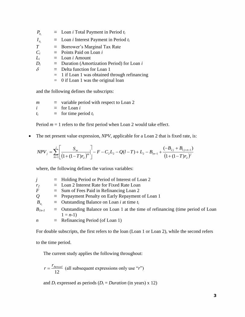
The net present value expression, NPV, applicable for a Loan 2 that is fixed rate, is:

j

njj

n

j

mm

m

jrT

BBBLTlQLCF

rT

SNPV

2

112

11222

1 2 )1(1

)()(

)1(1

where, the following defines the various variables:

j ≡ Holding Period or Period of Interest of Loan 2

r2 ≡ Loan 2 Interest Rate for Fixed Rate Loan

F ≡ Sum of Fees Paid in Refinancing Loan 2

Q ≡ Prepayment Penalty on Early Repayment of Loan 1

iitB ≡ Outstanding Balance on Loan i at time ti

B1n-1 ≡ Outstanding Balance on Loan 1 at the time of refinancing (time period of Loan

1 = n-1)

n ≡ Refinancing Period (of Loan 1)

For double subscripts, the first refers to the loan (Loan 1 or Loan 2), while the second refers

to the time period.

The current study applies the following throughout:

12

Annualrr (all subsequent expressions only use “r”)

and Di expressed as periods (Di = Duration (in years) x 12)

4

These substitutions assume all mortgage payments are monthly and require expressing n, m and

any other timing designation as periods. For example, if refinancing is considered in year 5, the

value for n is 60 (periods).

By inspection of Sm and NPV, the two expressions account for the tax deductibility of

interest payments, points costs amortization, and prepayment penalties. Also, the discount rate is

the new loan interest rate and is after-tax.

FRAMEWORK FOR MORTGAGE REFINANCING

The framework for this paper’s approach for assessing mortgage refinancing includes

establishing a common timeline for the original and new loan, defining (and accounting for) both

loan durations, providing scaling to generalize results, and developing explicit equations that

have similar timescales for the various terms in the per period savings and net present value

expressions.

Synchronizing Loan Timescales

Each loan has its own timeframe and periods – the first period of a refinanced loan is the nth

period of the original loan. Providing synchronized loan timescales establishes a common or

“real” time for all loan transactions.

For two fixed rate loans, Figure 1 shows the timing of payments and relationship between

the first and second loan. Illustrated in this figure, both period ti = n for Loan 1 and period m = 1

for Loan 2 refer to the first period for mortgage payments based on Loan 2 conditions, i.e., the

time period when mortgage refinancing would take effect. Thus, to reflect real time and to

synchronize the two loan time scales, the following defines the absolute time periods of Loans 1

and 2, t1 and t2, respectively:

mt

nmt

2

1 1

5

As required for derivations shown later in this paper, this time scale reduces time for both loans

to a single, synchronized variable, m, with the following limits:

At the point of refinancing: m = 0 (t1 = n - 1 & t2 = 0)

At the holding period: m = j (t1 = j + n – 1 & t2 = j)

Loan Durations

As shown in Figure 1, the duration for Loan 2 does not need to be the same or match the same

end date as the first loan. For the Loan 2, typical loan durations are:

duration)standard(anyD

DD

2

12

Scaling

This paper factors L1 from all per period and net present value terms to provide general

expressions. A simple example of this scaling occurs between L1 and L2:

12 LL L

This scaling establishes expressions that are independent of initial loan values (and apply

universally to all mortgage refinancing scenarios without loss of generality). This paper shows

this factoring or scaling throughout, while later presenting specific expressions for the loan scale

factor, L, and other scaling factors.

Explicit, Analytical Expressions For Per Period Savings Terms

For fixed-to-fixed rate loan refinancing, this work develops explicit expressions, using the

synchronized timescale and loan value scaling, for each component of the per period savings

expression, Sm: iititit C I P Biii,,, .

6

Loan Balance, iit

B . The general, explicit expression for iitB , at any time ti, is:

i

i

i

i D

i

t

it

iiitr

rrLB

11

111

The remaining balance for Loan 1, to any holding period: ti = t1 = m + n – 1, is:

1111

1

1

11

111111

111

nmBD

nmnm

nm Lr

rrLB

The remaining balance for Loan 2, to any holding period: ti = t2 = m, is:

mBLD

mm

m Lr

rrLB

221

2

2222

11

111

Loan Payment, iit

P . The loan payment is constant over the entire duration of a loan with a

fixed interest rate; therefore, we do not need a second, or time, subscript, as follows:

iiPiD

i

iii L

r

rLP

11

where:

iiti PP Loan i Total Payment in any period

For Loans 1 and 2, direct implementation of this general equation only requires

substitution of the appropriate ri and Di (and express both as a function of L1 and factor L1).

Interest Payment, iit

I . By identity, the interest payment depends directly on the interest rate

and remaining loan balance:

1ii itiit BrI

Rewriting this general expression by substituting for the respective remaining loan balance gives:

i

i

i

i D

i

t

it

iiiitr

rrLrI

11

111

11

7

Factoring and rearranging this expression provides:

11

111111

ii

i

ii

ii

tD

iPi

tD

iD

i

iiit rLr

r

rLI

The interest payment expression for Loan 1, to any holding period: ti = t1 = m+n-1, is:

2

11

2

1

1

1111

1

1

1

11111

11

nmD

P

nmD

Dnm rLrr

rLI

while, the interest payment expression for Loan 2, to any holding period: ti = t2 = m, is:

1

21

1

2

2

222

2

2

2

21111

11

mD

PL

mD

Dm rLrr

rLI

Points, Ci. The expression defining the relationship between points and loan values is:

1

1

2

21

1

11

2

12

1

11

2

22

D

C

D

CTL

D

TLC

D

TLC

D

TLC

D

TLC LL

In all cases, this expression is constant in time.

EXPLICIT, ANALYTICAL EXPRESSION FOR PER PERIOD SAVINGS, Sm

Updating the previous per period savings expression to reflect the appropriate subscripting for

synchronized time and loan values (to match the basis for the individual terms completed above)

gives:

1

11

2

22211211

D

TLC

D

TLCTIIPPS mnmmnmm

This form of the Sm expression allows the direct substitution of the explicit, analytical

expressions for the individual terms as developed above, giving:

1

1

2

21

1

2

2

11

1

2

2

1

1

21

1111

D

C

D

CTL

TrrL

LS

L

mD

PL

nmD

P

PLPm

8

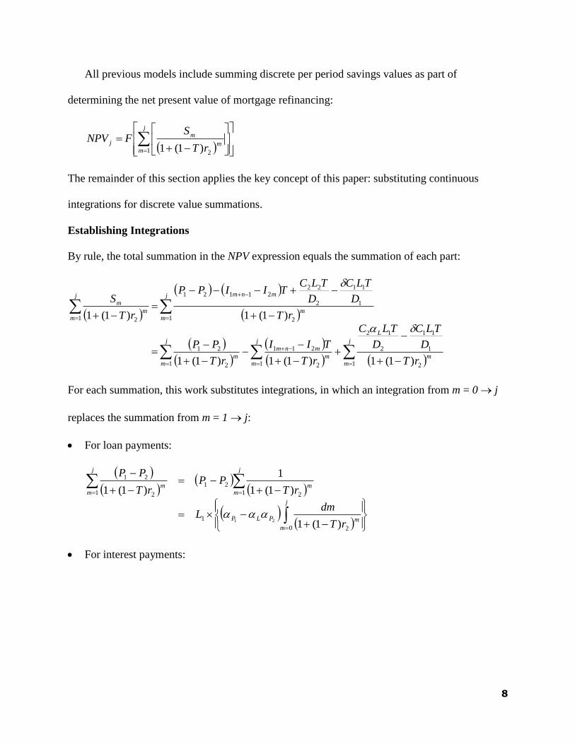
All previous models include summing discrete per period savings values as part of

determining the net present value of mortgage refinancing:

j

mm

m

jrT

SFNPV

1 2)1(1

The remainder of this section applies the key concept of this paper: substituting continuous

integrations for discrete value summations.

Establishing Integrations

By rule, the total summation in the NPV expression equals the summation of each part:

j

mm

L

j

mm

mnm

j

mm

j

mm

mnmj

mm

m

rT

D

TLC

D

TLC

rT

TII

rT

PP

rT

D

TLC

D

TLCTIIPP

rT

S

1 2

1

11

2

12

1 2

211

1 2

21

1 2

1

11

2

2221121

1 2

)1(1)1(1)1(1

)1(1)1(1

For each summation, this work substitutes integrations, in which an integration from m = 0 j

replaces the summation from m = 1 j:

For loan payments:

j

m

mPLP

j

mm

j

mm

rT

dmL

rTPP

rT

PP

0 2

1

1 2

21

1 2

21

)1(1

)1(1

1

)1(1

21

For interest payments:

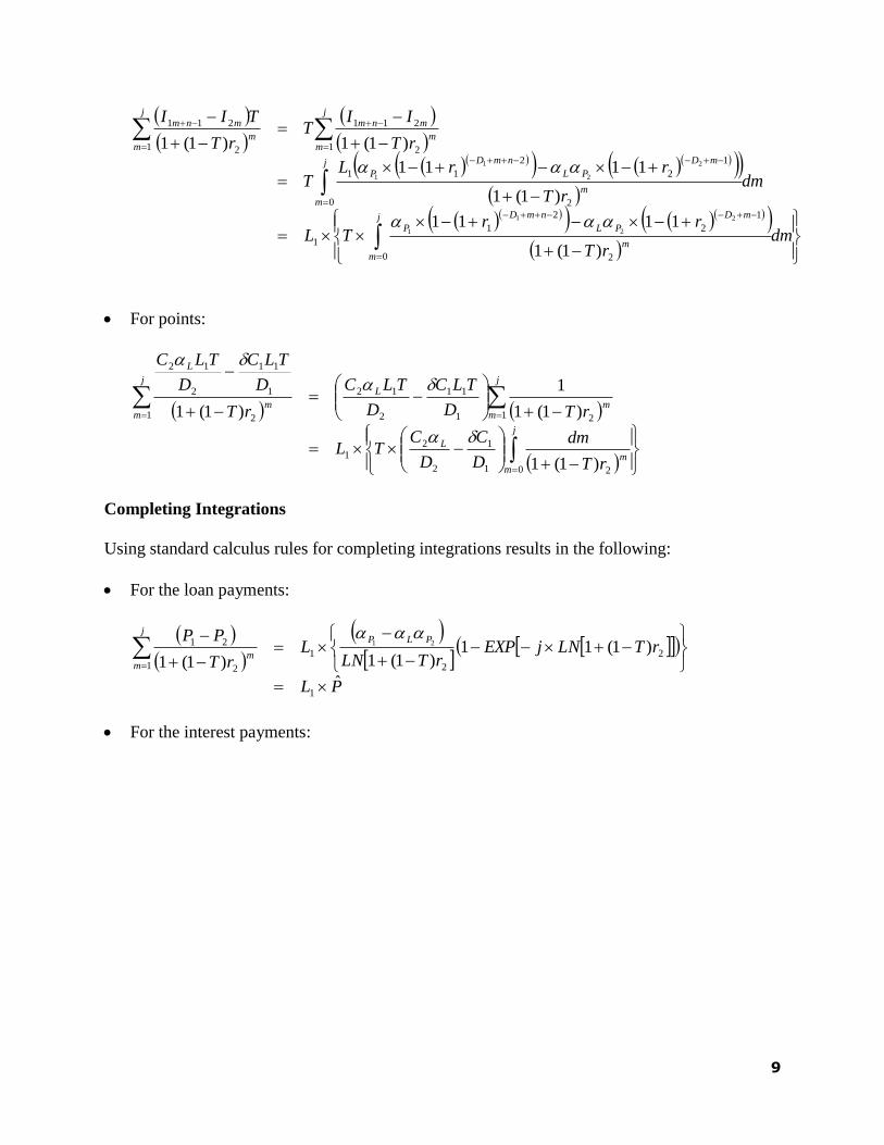
9

dmrT

rrTL

dmrT

rrLT

rT

IIT

rT

TII

j

m

m

mD

PL

nmD

P

j

m

m

mD

PL

nmD

P

j

mm

mnmj

mm

mnm

0 2

1

2

2

1

1

0 2

1

2

2

11

1 2

211

1 2

211

)1(1

1111

)1(1

1111

)1(1)1(1

2

2

1

1

2

2

1

1

For points:

j

m

m

L

j

mm

Lj

mm

L

rT

dm

D

C

D

CTL

rTD

TLC

D

TLC

rT

D

TLC

D

TLC

0 21

1

2

21

1 21

11

2

12

1 2

1

11

2

12

)1(1

)1(1

1

)1(1

Completing Integrations

Using standard calculus rules for completing integrations results in the following:

For the loan payments:

PL

rTLNjEXPrTLN

LrT

PP PLPj

mm

ˆ

)1(11)1(1)1(1

1

2

2

1

1 2

21 21

For the interest payments:

10

IL

rT

rLNjEXP

rT

rLN

r

rT

rLNjEXP

rT

rLN

r

rTLNjEXPrTLN

TLrT

TII

D

PL

nD

P

PLPj

mm

mnm

ˆ

1)1(1

11

)1(1

11

11

1)1(1

11

)1(1

11

11

)1(11)1(1)1(1

1

2

2

2

2

1

2

2

1

2

1

2

1

2

2

1

1 2

211

2

2

1

1

21

For the points:

CL

rTLNjEXPrTLN

D

C

D

C

TLrT

D

TLC

D

TLC L

j

mm

L

ˆ

)1(11)1(1)1(1

1

2

2

1

1

2

2

1

1 2

1

11

2

12

Now, these expressions provide a single value, through a single calculation, to account for the

summation of per period savings.

EXPLICIT, ANALYTICAL MATHEMATICAL EXPRESSIONS FOR NPV

The NPV equation contains additional terms that are added as singular values to the per period

savings summation. These terms require some manipulation to synchronize timescales and place

in a similar scaled form to match the framework of this work. When synchronized and scaled,

these form the various terms in the NPV expression.

Accounting for Remaining Balance Terms

The loan balance terms, B2j and B1j+n-1, do not involve any summations. We simply gather the

appropriate explicit expressions as developed earlier:

11

j

BBL

j

D

njnj

D

jj

L

j

njj

rTL

rT

r

rr

r

rr

LrT

BB

njj

2

1

2

1

1

11

1

2

22

1

2

112

)1(1

)1(1

11

111

11

111

)1(1

112

12

Accounting for Refinance Charges and Prepayment Penalties Terms

The refinance charges and prepayment penalties terms, F and Q, do not involve any summations.

We simply scale these terms:

1

1

LQ

LF

Q

F

Determining Values for the Loan Scale Factor, L

Utilizing the various expressions that have the scaling factor L requires a “correct” formula for

the scaling factor found from possible Loan 2 values. The following defines three possible values

for the new loan value:

j

njj

n

n

n

rT

BBBTQLCF

BTQLCF

BL

2

112

1122

1122

112

111

1

These expressions place bounds on possible Loan 2 values, where the first expression can be

considered a minimum and the third a maximum. The third expression appears unlikely –

especially because it requires a high level of confidence regarding the likely total duration of

holding the second loan. To simplify this work and to ensure that subsequent analyses reflect

typical refinancing, this paper only uses the first two expressions for possible Loan 2 values.

Using these two values for Loan 2, for fixed-to-fixed rate refinancing, this paper finds the

following loan scale factors:

12

1. For 111211

LBLn

Bn

, the resulting L expression is:

111

1

1

11

111

111

D

nn

BLr

rr

n

2. For 11222 1 nBTQLCFL , the Loan 2 value is:

2

1

2

11

21

1

1

111

C

TL

C

BTQFL n

BQFn

resulting in an L expression:

22

1

1

11

1

1

1

1

11

1111

11

1

C

T

C

r

rrT

nBQF

D

nn

QF

L

Using these two Loan 2 values and respective loan scale factors, the NPV expression for fixed-

to-fixed rate refinancing reduces to:

For 112 nBL :

j

njjj

mm

mj

rT

BBTQLCF

rT

SNPV

2

112

22

1 2 )1(1

)(1

)1(1

For 11222 1 nBTQLCFL , “ )(2 TlC QLF ” is removed:

j

njjj

mm

mj

rT

BB

rT

SNPV

2

112

1 2 )1(1

)(

)1(1

Complete NPV Expressions

The final forms for the NPV expressions are (with the appropriate loan scale factor, L, as given

above):

For 112 nBL :

13

j

D

njnj

D

jj

L

QLFj

rT

r

rr

r

rr

TlCCIPL

NPV

2

1

1

11

1

2

22

21

)1(1

11

111

11

111

)(ˆˆˆ

12

For 11222 1 nBTQLCFL :

j

D

njnj

D

jj

L

j

rT

r

rr

r

rr

CIPL

NPV

2

1

1

11

1

2

22

1

)1(1

11

111

11

111

ˆˆˆ

12

As noted throughout this paper and shown in these expressions, these explicit, analytical NPV

equations capture the total mathematics of refinancing for fixed-to-fixed rate mortgage

refinancing in a single calculation.

CONFIRMING THE ACCURACY OF THE DEVELOPED EXPRESSION

This work evaluates the accuracy of the developed explicit, analytical expressions by comparing

net present values generated by both the derived explicit, analytical expressions of this work and

the Tai and Przasnyski spreadsheet model for a series of refinancing cases. Table 2 lists the bases

for these refinancing cases and provides calculated NPV values for this work (NPVExplicit) and Tai

and Przasnyski (NPVSpreadsheet). While scaled values would show the same relative result (and sign)

for the NPV, in all cases, to provide actual dollar values, these analyses assign an initial value of

$100,000 to Loan 1.

14

The NPV data in this table show errors are insignificant between the two approaches –

less than 0.5% – resulting in less than $100 differences in the NPV of calculated savings. This

“error” falls well within the accuracy for rationally assessing refinancing decisions.

Additionally, the separate error resulting from using the derived expressions for Sm fell

below 0.3%.

CONCLUSION

This work shows the development of explicit, analytical expressions – with continuous

integrations replacing discrete summations – to complete mortgage refinancing calculations to

assess fixed-to-fixed rate mortgage refinancing. The results generated from this approach show

the derived expressions are highly accurate for calculating net present values when compared to

accepted models that implement discrete summations. The error in using the explicit, analytical

expressions generated in this work is less than 0.5% of results found using discrete summations.

With such low values for the error, this methodology may be superior to typical methods for

calculating the savings of mortgage refinancing, because this approach generates the net present

value in a single calculation.

15

Figure 1 Real Time Synchronization for Fixed-to-Fixed Rate Loans

Table 1

Analytical Models Determining Mortgage Refinancing Benefit

Reference

Sa

vin

gs =

Mo

rtga

ge

Pa

ym

ent R

edu

ction

Befo

re-T

ax

PV

of A

ll

Refin

an

cing

Co

sts

Ca

sh F

low

Cu

rren

t Va

lue

Av

era

ge P

ay

men

t

Disco

un

t Ra

te N

ew L

oa

n

Inte

rest R

ate

Befo

re-T

ax

Disco

un

t Ra

te

Fix

ed R

ate

Ad

justa

ble R

ate

Ta

x B

enefits o

f Inte

rest

Pa

ym

ents

No

n-D

edu

ctible

Refin

an

cing

Co

sts

Am

ortiza

tion

an

d T

ax

Ben

efits of P

oin

ts

NP

V A

na

lysis o

f Ca

sh

Flo

ws

Disco

un

t Ra

te = N

ew L

oa

n

Inte

rest R

ate

After

-Ta

x D

iscou

nt R

ate

Lo

an

s’ Ou

tstan

din

g

Ba

lan

ces Differ

ence

Sto

cha

stic Inte

rest R

ate

Lipscomb (1983)

16

Table 1

Analytical Models Determining Mortgage Refinancing Benefit

Reference

Sa

vin

gs =

Mo

rtga

ge

Pa

ym

ent R

edu

ction

Befo

re-T

ax

PV

of A

ll

Refin

an

cing

Co

sts

Ca

sh F

low

Cu

rren

t Va

lue

Av

era

ge P

ay

men

t

Disco

un

t Ra

te N

ew L

oa

n

Inte

rest R

ate

Befo

re-T

ax

Disco

un

t Ra

te

Fix

ed R

ate

Ad

justa

ble R

ate

Ta

x B

enefits o

f Inte

rest

Pa

ym

ents

No

n-D

edu

ctible

Refin

an

cing

Co

sts

Am

ortiza

tion

an

d T

ax

Ben

efits of P

oin

ts

NP

V A

na

lysis o

f Ca

sh

Flo

ws

Disco

un

t Ra

te = N

ew L

oa

n

Inte

rest R

ate

After

-Ta

x D

iscou

nt R

ate

Lo

an

s’ Ou

tstan

din

g

Ba

lan

ces Differ

ence

Sto

cha

stic Inte

rest R

ate

Buser and

Henderschott (1984)

Hall (1985)

Waller (1987)

G-Yohannes (1988)

Marquardt and

Woerheide (1988)

Follain and Tzang

(1988)

Chen and Ling

(1989)

Richard and Roll

(1989)

Followill and

Johnson (1989)

Kirby, Nash and

Stanford (1990)

Rose (1992)

Follain, Scott and

Yang (1992)

Yang and Maris

(1993)

Arsan and

Poindexter (1993)

Tai and Przasnyski

(1996)

Timmons and Betty

(1997)

Hoover (2003)

Johnson and Randle

(2003)

Fortin et al. (2005)

and (2007)

Table 2

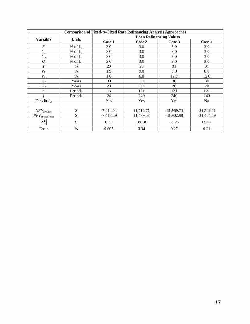
17

Comparison of Fixed-to-Fixed Rate Refinancing Analysis Approaches

Variable Units Loan Refinancing Values

Case 1 Case 2 Case 3 Case 4

F % of L1 3.0 3.0 3.0 3.0

C1 % of L1 3.0 3.0 3.0 3.0

C2 % of L1 3.0 3.0 3.0 3.0

Q % of L1 3.0 3.0 3.0 3.0

T % 20 20 31 31

r1 % 1.9 9.0 6.0 6.0

r2 % 1.0 6.0 12.0 12.0

D1 Years 30 30 30 30

D2 Years 28 30 20 20

n Periods 13 121 121 121

j Periods 24 240 240 240

Fees in L2 Yes Yes Yes No

NPVExplicit $ -7,414.04 11,518.76 -31,989.73 -31,549.61

NPVSpreadsheet $ -7,413.69 11,479.58 -31,902.98 -31,484.59

$ $ 0.35 39.18 86.75 65.02

Error % 0.005 0.34 0.27 0.21